1 Visibility in Computer Graphics Toni Sellarès Unversitat de Girona.

1

Visibility in Computer Graphics

Toni SellarèsUnversitat de Girona

2

Visibility

Two points of a scene are mutually visible if the line segment connecting them is unoccluded.

3

Visibility

Visibility problems can be classified based on the problem domain

4

Visibility taxonomy (*)

1. visibility along a line

2. visibility from a point

3. visibility from a line segment

4. visibility from a polygon

5. visibility from a region

6. global visibility

(*) J. Bittner, P. Wonka, Visibility in Computer Graphics, Journal of Environment and Planning B: Planning and Design, vol. 30. no. 5, pp 729 – 725, 2003

5

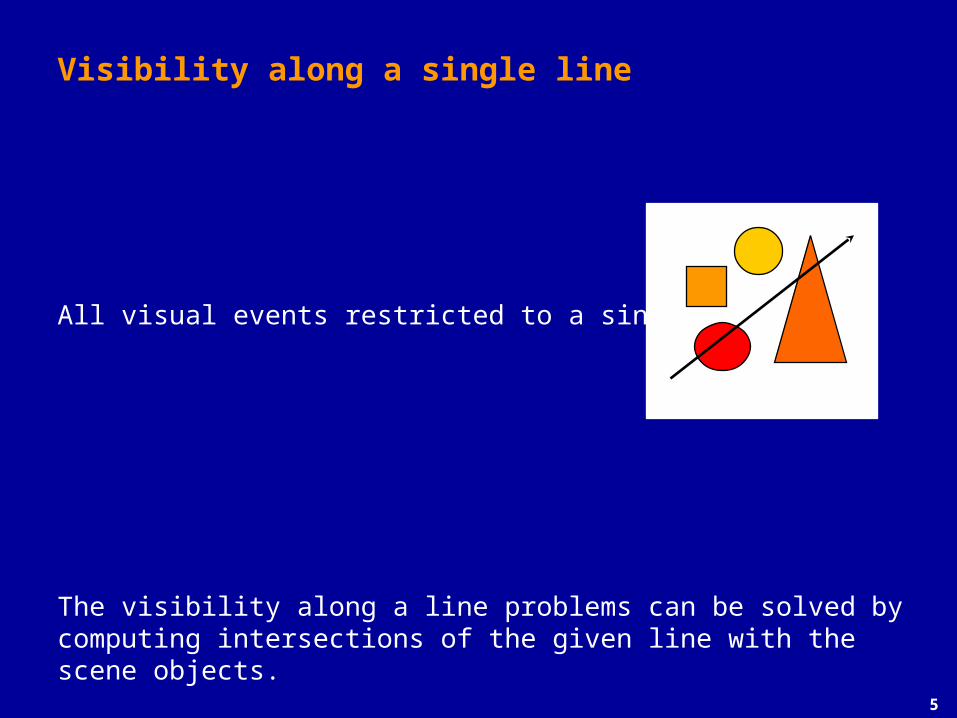
Visibility along a single line

All visual events restricted to a single line.

The visibility along a line problems can be solved by computing intersections of the given line with the scene objects.

6

Visibility along a single line

• Point-to-point visibility determines whether the line segment between two points is unoccluded, i.e. the line segment has no intersection with an object in the scene.

• Ray shooting: given a ray, determine the first intersection of the ray with a scene object.

7

Visibility from a point

Is the classical visible surface determination problem.

Due to its importance for image synthesis, visible surface determination (hidden-surface removal) covers the majority of existing visibilty algorithms in computer graphics.

8

Visibility from a region

Is a most general problem.

• Region-to-region visibility problem determines if the two given regions in the scene are mutually visible, invisible or partially visible.

• Other examples:

– potentially visible sets,

– aspect graph,

– 3D visibility complex

9

• When a 3-dimensional scene description is transformed to screen coordinates by a projection transformation, more than one object may overlap the same sample in the image.

• Some method is needed to determine which is the visible one,

so that pixels can be shaded appropriately.

Hidden-surface removal

10

Object-Space Methods

• Use geometric tests on the object descriptions to determine which objects overlap and where.

• Object space algorithms are O(n2) where n is the number of objects in the scene.

• Complexity of algorithms is high, few primitives are supported, and special effects often are difficult to implement

Examples: painter's algorithms, depth-sorting, BSP

11

Image-Space Methods

• Many approaches take advantage of the discretized nature of the output image, computing visibility only to the precision required to decide what is visible at a particular pixel.

• Image space algorithms are O(nN) where n is the number of objects in the scene and N is the number of pixels.

• Allow more advanced effects and complex models.

Examples: z-buffer, Watkin's, ray-casting

12

Why might a polygon (face) be invisible ?

– Polygon outside the field of view

– Polygon is backfacing

– Polygon is occluded by object(s) nearer the viewpoint

• We want to avoid spending work on polygons outside field of view or backfacing

• We need to know when polygons are occluded

13

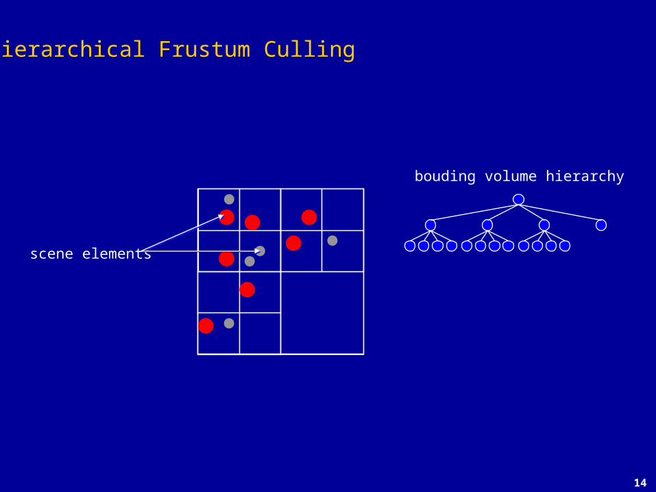
Frustun culling

• Quickly reject what is not visible

• Conservative: never classify a visible scene element as invisible

• Reduce unecessary processing

14

bouding volume hierarchy

scene elements

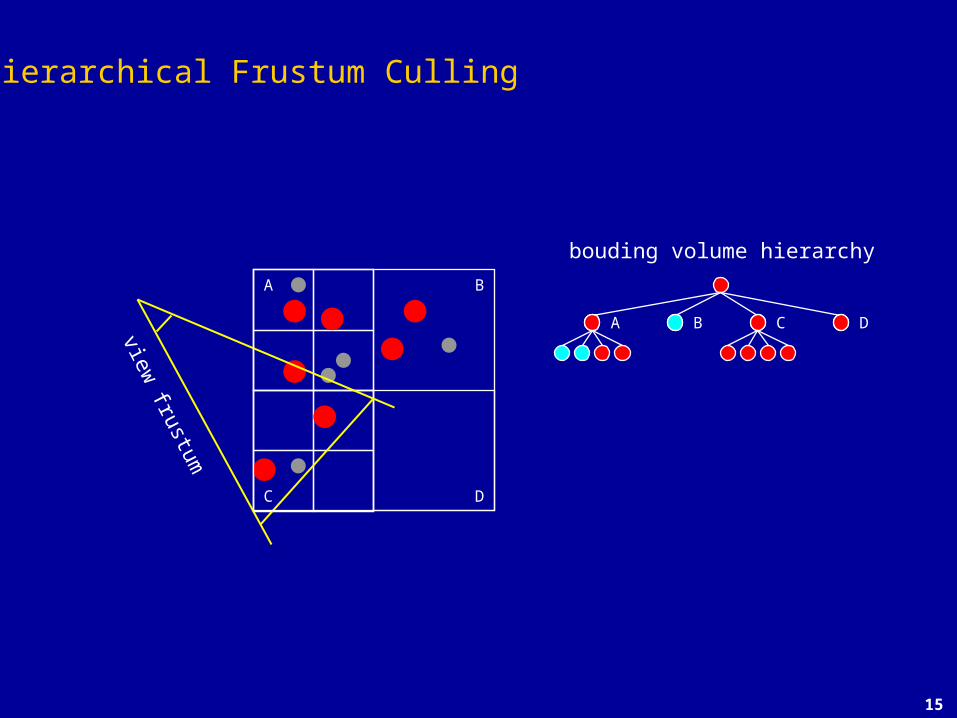
Hierarchical Frustum Culling

15

bouding volume hierarchy

view frustum

A B

DC

BA C D

Hierarchical Frustum Culling

16

Backface Removal (Backface Culling)

• Removes entire polygons that face away from the viewer

• If we are dealing with a single convex object, culling completely solves the hidden surface problem

Geometric test for the visibility

surface visible: 0NVVN

surface invisible : 0NV

silhouette : 0NV

17

Back-Face Culling

• On the surface of an object, polygons whose normals point away from the camera are always occluded:

Note: backface cullingalone doesn’t solve the

hidden-surface problem!

18

Back-Face Culling

• Not rendering backfacing polygons improves performance

• Reduces by about half the number of polygons to be considered for each pixel

19

Occlusion

• For most scenes, some polygons will overlap:

• To render the correct image, we need to determine which polygons occlude which

20

Conservative occlusion testing

• If the box representing a node is not visible then nothing in it is either• The faces of the box are projected onto the image plane and tested

for occlusion

occluder

hierarchicalrepresentation

21

Testing a Node for Occlusion

• If the box representing a node is not visible then nothing in it is either• The faces of the box are projected onto the image plane and tested for

occlusion

occluder

hierarchicalrepresentation

22

Occlusion Removal Algorithms

• Painter’s Algorithm Hybrid

• BSP tree Algorithm Hybrid

• Z-Buffer Algorithm Image-space

• Ray-Casting Algorithm Object-space

23

Painter's Algorithm

– Sort all polygons according to the (farthest) z coordinates of each,

– When the polygon's z extents overlap, resolve the sorting ambiguities by splitting the polygons

– Draw (fill) the polygons in the sorted order– back to front

• Also known as Depth-sort algorithm.

24

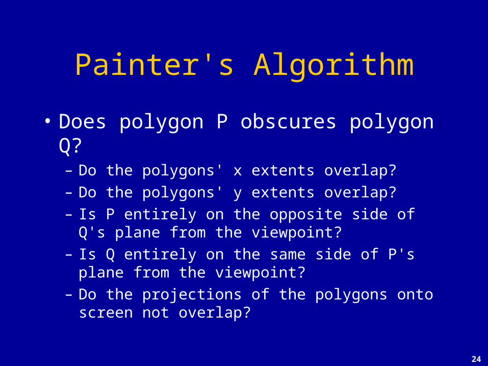
Painter's Algorithm

• Does polygon P obscures polygon Q?– Do the polygons' x extents overlap?– Do the polygons' y extents overlap?– Is P entirely on the opposite side of Q's plane from

the viewpoint?– Is Q entirely on the same side of P's plane from

the viewpoint?– Do the projections of the polygons onto screen not

overlap?

25

Painter’s Algorithm

Some cases in which Z extents of polygons overlap

Z

X X X

YY

26

Binary Space Partitioning Tree Algorithm

• Very efficient for a static group of 3D polygons as seen from an arbitrary viewpoint

• Correct order for Painter’s algorithm is determined by a suitable traversal of the binary tree of polygons: BSP Tree

27

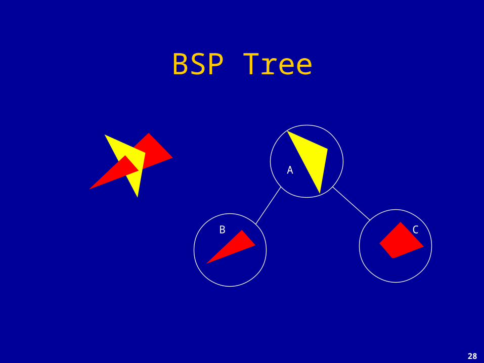
BSP Tree

28

BSP Tree

A

B C

29

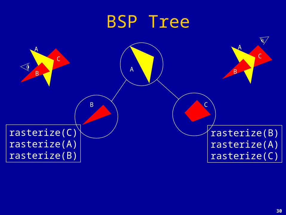
BSP Tree

tree.root

tree.left

Draw BSP Treefunction draw(bsptree tree, point eye)if tree.empty then

returnif ftree.root(eye) < 0

draw (tree.right)rasterize(tree.root)draw(tree.left)

else draw (tree.left)rasterize(tree.root)draw(tree.right)

tree.right

30

BSP Tree

A

B C

rasterize(C)rasterize(A)rasterize(B)

B

C

A

rasterize(B)rasterize(A)rasterize(C)

CA

B

31

BSP Tree

• Code works for any view

• Tree can be pre-computed

• Requires evaluation of

fplane of the triangle(eye)

32

BSP Tree Construction

• The binary tree is constructed using the following principle:– For each polygon, we can divide the set of other

polygons into two groups– One group contains those lying in front of the

plane of the given polygon– The other group contains those in the back– The polygons intersecting the plane of the given

polygon are split by that plane

33

Summary: BSP Trees

• Pros:– Simple, elegant scheme– Only writes to framebuffer (i.e., painters algorithm)

• Thus very popular for video games (but getting less so)

• Cons:– Computationally intense preprocess stage restricts

algorithm to static scenes– Worst-case time to construct tree: O(n3)– Splitting increases polygon count

• Again, O(n3) worst case

34

Z-Buffer Algorithm

• Color values are stored in a frame buffer.

• We also need a z-buffer, of the same size as the frame

buffer, to store z value of each image pixel.

Frame-Buffer

Z-Buffer

35

-far-far-far-far-far-far-far-far-far-far-far-far

fram

ebuf

fer

zbuf

fer

Z-Buffer Algorithm

• Key Observation: Each pixel displays color of only one polygon, ignores everything behind it.

• Don’t need to sort polygons, just find for each pixel the closest triangle.

• Z-buffer: one fixed or floating point value per pixel.

36

-far-.1-.2-.3-.4-.5-.6-.7-.8-far-far-far

fram

ebuf

fer

zbuf

fer

Z-Buffer Algorithm




37

-far-.1-.2-.3-.4-.3-.1-.7-.8-far-far-far

fram

ebuf

fer

zbuf

fer

Z-Buffer Algorithm




38

-far-.1-.2-.3-.4-.3-.1-.7-.8-far-far-far

fram

ebuf

fer

zbuf

fer




Z-Buffer Algorithm

39

Z-Buffer Pseudo-code

For each rasterized fragment (x,y)

If z > zbuffer(x,y) then

framebuffer(x,y) = fragment color

zbuffer(x,y) = z

40

Ray CastingFind nearest surface along the view ray (ray shooting).

eye

for i = 0 to nRows-1 for j = 0 to nCols-1 ray = genRay(eye, pixel(i,j)) castRay(ray)

41

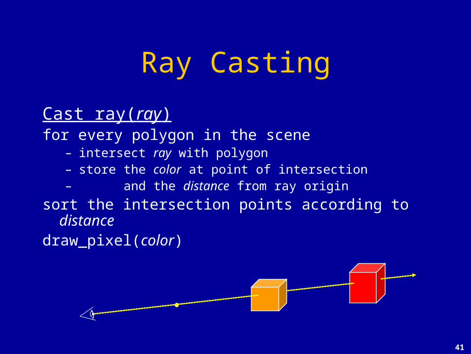
Cast ray(ray)for every polygon in the scene

– intersect ray with polygon– store the color at point of intersection– and the distance from ray origin

sort the intersection points according to distancedraw_pixel(color)

Ray Casting

42

Ray CastingFind nearest surface along the view ray (ray shooting).

eye

for i = 0 to nRows-1 for j = 0 to nCols-1 ray = genRay(eye, pixel(i,j)) castRay(ray)

43

Ray Casting

WW UU

VV

eye

44

Ray Casting

WW

UU

VV

eye

1 Visibility in Computer Graphics Toni Sellarès Unversitat de Girona.

Documents

Transcript of 1 Visibility in Computer Graphics Toni Sellarès Unversitat de Girona.