


Languages
Pages
Legal


UNIVERSITEIT GENT
FACULTEIT ECONOMIE EN BEDRIJFSKUNDE
ACADEMIEJAAR 2012 – 2013
MACROECONOMIC CONSENSUS DATA AND FINANCIAL MARKETS
Masterproef voorgedragen tot het bekomen van de graad van
Master of Science in de Toegepaste Economische Wetenschappen: Handelsingenieur
Mathias Wambeke
onder leiding van
Prof. Dr. William De Vijlder

I
PERMISSION
The undersigned declares that the content of this thesis can be consulted and/or reproduced, subject
to acknowledgement of sources.
Mathias Wambeke

II
PREFACE
When writing this thesis, I had help from multiple sources. First of all, I would like to thank Prof. Dr.
William De Vijlder for his ongoing advice and support with this subject. Also, a word of thanks to
Kristjan Kasikov (foreign exchange quantitative analyst at Citigroup) for providing me with additional
data.

III
TABLE OF CONTENTS
PREFACE .................................................................................................................................................. II
TABLE OF CONTENTS .............................................................................................................................. III
ABBREVIATIONS ....................................................................................................................................... V
LIST OF TABLES ........................................................................................................................................ V
LIST OF FIGURES ..................................................................................................................................... VI
I. INTRODUCTION ............................................................................................................................... 1
II. MACROECONOMIC SURPRISES........................................................................................................ 3
II.1. Current literature ......................................................................................................................... 3
II.1.1. Research on the macroeconomic fundamentals of asset returns ........................................ 3
II.1.2. Research on macro surprises and asset returns ................................................................... 7
II.1.3. Surprise indices.................................................................................................................... 13
II.2. Data and descriptive analysis ..................................................................................................... 14
II.2.1. Data ..................................................................................................................................... 14
II.2.2. Descriptive analysis ............................................................................................................. 16
II.3. Method and results .................................................................................................................... 20
II.3.1. Surprise indices and long term government bond returns ................................................. 21
II.3.2. Timing government bond portfolios ................................................................................... 22
II.4. Conclusion .................................................................................................................................. 26
III. DISPERSION & CONSENSUS DATA ............................................................................................. 28
III.1. Current literature ...................................................................................................................... 28
III.1.1. Dispersion of micro consensus data ................................................................................... 28
III.1.2. Dispersion of macro consensus data .................................................................................. 31
III.1.3. Pricing models and the dispersion – asset return relationship .......................................... 35
III.1.4. Gaps in current research .................................................................................................... 36
III.2. Data ........................................................................................................................................... 38
III.3. Method and results ................................................................................................................... 42
III.3.1. Stock returns and macro dispersion ................................................................................... 42
III.3.2. Forecast errors and macro dispersion ................................................................................ 45
III.3.3. Default premia and macro dispersion ................................................................................ 47
III.3.4. Preliminary conclusion ....................................................................................................... 50
III.4. Conclusion ................................................................................................................................. 51
REFERENCES .......................................................................................................................................... VII
IV
APPENDIX ............................................................................................................................................. XIII
Appendix 1 - Out of sample bond timing returns for different derivatives ................................. XIII
Appendix 2 –Bond timing strategy based on US and domestic surprise index derivatives ......... XVI
Appendix 3 - Unit root tests ........................................................................................................ XVII
Appendix 4 –Bond timing strategy based on surprise index levels ............................................ XVIII
Appendix 5 – Chow breakpoint tests ........................................................................................... XIX
Appendix 6 – Market timing for the S&P500 based on macro dispersion .................................... XX
Appendix 7 – Plot of disagreement on TBOND and 6 month S&P500 returns ............................ XXI
Appendix 8 – Granger causality tests ........................................................................................... XXI
Appendix 9 – Market timing for the default premium based on macro dispersion ................... XXII
Appendix 10 – Plot of disagreement on CPI and the 1 month default spread change .............. XXIII
Appendix 11 – Nederlandse samenvatting ................................................................................ XXIV

V
ABBREVIATIONS
ADS Aruoba – Diebold - Scotti index
CESI Citi Economic Surprise Index
CESICAD Canada Citi Economic Surprise Index
CESIEUR EMU area Citi Economic Surprise Index
CESIGBP UK Citi Economic Surprise Index
CESIJPY Japan Citi Economic Surprise Index
CESIUSD USA Citi Economic Surprise Index
ECB European Central Bank
HML High Minus Low – book to market factor
SMB Small Minus Big – size factor
SPF Survey of Professional Forecasters
UMD Up Minus Down – momentum factor
LIST OF TABLES
Table 1; Early studies on asset returns and macroeconomic variables .................................................. 3
Table 2; macroeconomic surprises and stock returns............................................................................. 8
Table 3; macroeconomic surprises and foreign exchange returns ......................................................... 9
Table 4; macroeconomic surprises and fixed income returns .............................................................. 11
Table 5; correlations between Citi Economic Surprise Indices ............................................................. 15
Table 6; long term government bond portfolios ................................................................................... 15
Table 7; money market rates ................................................................................................................ 16
Table 8; correlations between 3 month % forex returns and surprise indices ..................................... 18
Table 9; correlations between surprise indices and 3 month % returns of long term government
bonds ..................................................................................................................................................... 20
Table 10; Regressions of bond returns on surprise indices ................................................................... 21
Table 11; Market timing statistics ......................................................................................................... 25
Table 12; Philadelphia SPF macroeconomic estimates ......................................................................... 38
Table 13; correlations between dispersion measures .......................................................................... 41
Table 14; regressions of excess stock returns on macro disagreement ............................................... 42
Table 15; market timing for the S&P500 based on macro dispersion .................................................. 44
Table 16; regressions of absolute forecast errors on macro disagreement ......................................... 45
Table 17; regressions of absolute forecast errors on NBER recessions and macro disagreement ....... 46
Table 18; regressions of default premia on GDP growth, VIX and macro disagreement...................... 47
Table 19; default premium regressed on its macro determinants ....................................................... 49
Table 20; market timing for the default spread based on macro dispersion ........................................ 50

VI
LIST OF FIGURES
Figure 1; CESIUSD and S&P500 returns ................................................................................................. 17
Figure 2; CESIUSD and Euro Stoxx 50 returns ....................................................................................... 17
Figure 3; CESIEUR-CESIUSD and EURUSD returns ................................................................................. 18
Figure 4; CESIUSD-CESIJPY and USDJPY returns .................................................................................... 18
Figure 5; CESIUSD and 3 month log returns of a 30 year T bond portfolio ........................................... 19
Figure 6; CESIUSD and 3 month log returns of a 30 year EMU bond portfolio ..................................... 19
Figure 7; different measures of dispersion. .......................................................................................... 32

1
I. INTRODUCTION
Macroeconomic consensus data are pooled estimates or predictions on variables that have the
potential to determine the current state of the economy. These predictions are provided by banks or
forecasting departments of large industrial companies, and aggregated trough services such as
Bloomberg.
Although decent macro consensus data were almost non-existent about twenty years ago, they have
now gained considerable importance in financial markets and academic research. The reason for this
is quite straightforward; raw macro releases do not provide enough information to trade, as financial
markets only react to unexpected components of news. Therefore, it will be the difference between
macro releases and the corresponding consensus that will be determinant on the reaction of
investors. Indeed, simple macroeconomic releases do provide insight into the overall state of the
economy, but they aren’t useful for financial markets unless they are considered simultaneously with
their respective consensus estimates.
The increasing interest of financial market actors in macro consensus estimates is clearly linked to
the wide availability of this type of data. For example, Bloomberg now provides a large set of pooled
USA macro estimates, ranging from GDP growth rates and nonfarm payrolls to unit labor costs.
Reviews dedicated solely to macro consensus data have emerged, e.g. ConsensusEconomics®.
Central banks are also clearly interested in macro estimates; both the ECB and the Federal Reserve
Bank of Philadelphia now manage their own Survey of Professional Forecasters (SPF).
Literature dealing with the effect of macroeconomic surprises1 on asset markets has become quite
mature over time. Numerous studies have shown that financial markets (including stock markets,
fixed income and forex) react to the surprise of macro releases. These researches often apply
sophisticated econometric models (see for example Andersen, Bollerslev, Diebold and Vega, 2003)
and managed to get, over time, some agreement on which macro surprises affect asset markets
under which conditions (cf. supra).
Another interesting application of macro consensus data resides in its potential to proxy for
uncertainty. Arnold and Vrugt (2008) and Glansbeek and Ivo (2011) use the dispersion of macro
estimates to establish a link between volatility in financial markets and macroeconomic uncertainty.
Furthermore, Dopke and Fritsche (2006) find that macro uncertainty is particularly high before and
during recessions.
In this thesis, multiple gaps in current literature on macro consensus data are identified. First of all,
the market timing potential of macro surprise indices will be assessed. These indices aggregate the
surprises of multiple macroeconomic series into a comprehensive surprise measure. Although this
1 defined as the standardized difference between a macro release and the corresponding consensus
estimate

2
type of data provides an interesting way of dealing with the surprise of macro consensus estimates,
it has hardly been discussed in literature so far.
A second gap in extant research is the application of macroeconomic uncertainty in relationship to
stock returns. The past use of dispersion in macro consensus data was limited to assessing its impact
on asset volatility or other more descriptive approaches. In thesis, it will be verified whether this
macro uncertainty is a measure of non-diversifiable risk, and whether it is therefore linked to
innovations in stock markets. Furthermore, dispersion in macro estimates will be used in two other
domains; we will check how dispersion and macro surprises are related, and whether macro
uncertainty can explain default premia.
The structure of this thesis is as follows; the first part will deal with macro surprises and starts with
an overview of current literature about the effect of macro variables, macro surprises and macro
surprise indices on asset prices. Subsequently, data and descriptive analysis are provided, followed
by market timing models for government bonds based on macro surprise indices. Next, the results
and preliminary conclusion are given.
The second part of this thesis will deal with the dispersion of consensus estimates. It starts with an
overview of related literature on micro and macro consensus data, after which multiple gaps in
current research are identified. Subsequently information is provided on consensus forecasts
obtained from the Philadelphia SPF. The following section describes our econometric models and
provides the results; the last part concludes.
In the next pages, this thesis will present that macro surprise indices have the potential of
determining a profitable market timing strategy for long term government bonds, though to a limited
extent. Also documented is a clear effect of macro dispersion on subsequent surprises and default
premia. However, the dispersion of macroeconomic consensus data does not appear to have a clear
relationship to stock returns, nor can it be used for a stock market timing or default premium timing
strategy.
3
II. MACROECONOMIC SURPRISES
II.1. Current literature
This literature overview starts with some early studies on the link between asset returns and macro
fundamentals. Next, a review of papers studying the effect of macro surprises on stock, forex and
bond returns is provided. The section ends with some notes on macro surprise indices. Unless
mentioned otherwise, results are reported for US markets and US macro variables.
II.1.1. Research on the macroeconomic fundamentals of asset returns
II.1.1.1. Stock markets
The first articles on the link between stock returns and macro variables were published around the
year 1980. These early studies simply used regressions of asset returns on current, lagged or future
innovations of macro variables. There is a large discrepancy in the conclusions of the researches
applying this method, with some authors revealing significant coefficients for macro variables (e.g.
Fama, 1990), while others admit having discovered no relationship at all (e.g. Cutler, Poterba, and
Summers, 1989). Many authors discern a significant negative relationship between inflation, interest
rates and stock returns, while evidence for real activity measures (industrial production, GNP) is
mixed at best. The table below provides a short overview of these early publications.
Table 1; Early studies on asset returns and macroeconomic variables
Note; (+) indicates a positive relationship with stock returns, (-) indicates a negative relationship,
(0) indicates no relationship
Author (year of publication) Coefficients evaluated
C.R. Nelson (1976) Inflation (-)
Fama, G.W. Schwert (1977) Inflation (-)
Fama (1981) Inflation (-), future capital expenditures (+), future
industrial production (+), future real GNP (+)
Solnick (1984) Interest rates (-)
Kaul (1987) Inflation (-), M1 (-),industrial production (+), real GDP (+)
Asprem (1989) Employment (-), imports (-), inflation (-) interest rates (-
), future industrial production (+), capital expenditures
(0)), measures for money supply (+) and the U.S. yield
curve (+), consumption (0)
Fama and French (1989) Default premium (+), term premium (+)
Cutler, Poterba, Summers, 1989 Industrial production (0), CPI (0), M1 (0), long-term
interest rates (0), 3 month t bill rate (0)
Wasserfallen (1989) Real GNP (0), Industrial production (0), real consumption
(0), real investment (0), consumer prices (0), money

4
supply (0), monetary base (0), real exports (0), import
prices (0), nominal interest rate (0), real interest rate (0).
Fama (1990) Default premium (+), term premium (+), future industrial
production(+)
Schwert (1990) Future industrial production (+)
Balvers, Cosimano, McDonald
(1990)
Industrial production (-)
Chen (1991) Past GNP (-), future GNP (+), term structure (+), default
spread (+), industrial production (-), t bill rate (-),
dividend yield (+)
Marathe and Shawky (1994) The permanent component of industrial production (-)
Conover, Jensen, Johnson (1999) Central bank discount rates (-)
Durham (2001) discount rate (0) (measured in nominal and real terms, as
well as spread with a 3 month t bill), M1 growth (0)
Fifield, D.M. Power, C.D. Sinclair
(2000)
GDP, inflation, money supply, interest rates, world
industrial production and world inflation
Rapach, Wohar, Rangvid (2005) Money market rate (-), 3-month Treasury bill rate (-),
long-term government bond yield (-), term spread (0),
inflation rate (-), industrial production (0), narrow money
(0), broad money (0), unemployment rate (0)
Ang and Bekaert (2007) Short term interest rate (-)
Over time, more advanced methods have been developed to assess the stock market – macro
variables relationship. Vector autoregression (VAR) is one such novel technique that was introduced
about two decades ago in this research area. For example, Lee (1992) uses a VAR to find that
industrial production granger causes stock returns, while no relationship was discovered between
stock returns and inflation. Kaneko and Lee (1995) also employ a VAR analysis and establish that
risk premia, term premia and industrial production are significant for predicting US stock returns,
whereas inflation is only slightly important.
Cointegration analysis is another often used approach to examine the link between stock markets
and economic variables. If two variables are cointegrated, their long term equilibrium relationship,
as well as the corresponding error correction model (ECM) can be established through a regression.
For example, Siklos and Kwok (1999) use a cointegrating VAR and find a negative relationship
between stock returns and inflation. They argue that this result is driven by central bank debt
monetization. Nasseh and Strauss (2000) demonstrate trough cointegration analysis that stock
returns are significantly related to industrial production (+), business surveys of manufacturing
orders (+) , short-term interest rates (+), long-term interest rates (-) and CPI (+). Likewise, Humpe
and Macmillan (2009) show that stock returns are related to industrial production (+), the long term
interest rate (-) and CPI (-). Binswanger (2004) however, argues that for the longer 1950-2000
5
period, no clear cointegrating relationship can be found in G-7 countries for real GDP, industrial
production, and stock returns.
A recent strand in literature searches for regime dependent macro effects on stock returns. An often
used approach is to construct a two state Markov model for stock returns, which in practice almost
always results in a high return – low variance and a low return – high variance regime. Next, the
influence of macro variables on stock returns is assessed for each of the two regimes, (potentially)
together with the effect of macro variables on transition probabilities. For example, Perez-Quiros and
Timmermann (2000) find a significant influence of the 1 month t bill rate (-) and default premium
(+) during the low return – high variance regime, while these variables don’t affect stock returns
during high return – low variance periods. Similarly, Chang (2009) finds that the 3 month t bill rate
(-) and default premium (+) significantly affects stock markets during the low return – high volatility
regime, but not so for high return – low volatility periods. Chen (2007) shows that M2 growth (+),
the federal funds rate (-) and discount rate (-) significantly affect stock markets, but this relationship
appears to be stronger during bear market regimes. Furthermore, it is shown that decreasing
discount rates lead to a higher probability of switching to a bear-market period.
In summary, there is a vast amount of literature available on the link between macroeconomic factors
and stock market returns. Although multiple authors find a significant relationship between inflation
(-), interest rates (-) and stock returns, results for measures of real economic activity (industrial
production, GDP, employment etc.) are mixed at best. It could be argued that this lack of clarity is
partially due to the fact that only a limited number of papers take into account time varying
coefficients for macro variables. Moreover, all of the above papers ignore the existence of consensus
data. This seems problematic, as classic investment theory states that asset prices only respond to
the unexpected component of (macroeconomic) news. Therefore, only taking into account macro
series without their respective consensus estimates seems like an invalid measure of macroeconomic
influences, therefore making spurious data mining results likely. The next section (II.1.2) will thus
pay considerable attention to researches that do take into account macro surprises, not just raw
macroeconomic announcements.
II.1.1.2. Foreign exchange
Most of the research about macroeconomic effects on forex rates has focused on the so-called
fundamental models. These include (i) the flexible price monetary model, (ii) sticky price monetary
model, (iii) the productivity differential model and (iv) models based on the Taylor rule.
The flexible price (Frenkel-Bilson) model defines an exchange rate as the relative price resulting from
the demand and supply for two moneys. Other key assumptions made by this model include that (1)
domestic and foreign assets are perfect substitutes; (2) purchasing power parity (PPP) holds at all
times; and (3) the uncovered interest parity (UIP) holds at all times. The resulting model is given
by;
s = a0 + a1*(m-mf) + a2(y-yf) + a3*(rs-rsf) + u

6
where s is the logarithm of the domestic price of foreign currency, m is the logarithm of money
supply, y is the logarithm of real income, rs is the short-term interest rate, and u is an error term.
The subscript f indicates foreign variables.
The sticky-price (Dornbusch-Frankel) model does not assume the PPP to hold continuously; the goods
market prices are presumed to be sticky, at least in the short run. Exchange rates and interest rates
therefore have to compensate for this price stickiness, and thus exchange rates can “overshoot” their
long-run equilibrium rates. The resulting equation is given by;
s = a0 + a1*(m-mf) + a2(y-yf) + a3*(rs-rsf) + a4*(e-ef) + u
wheree is the expected long-run inflation.
The alternative sticky price (Hooper-Merton) model also allows the long-run real exchange rate to
fluctuate. These real exchange rate changes are presumed to be caused by unanticipated trade
balance shocks. The resulting equation is;
s = a0 + a1*(m-mf) + a2(y-yf) + a3*(rs-rsf) + a4*(e-ef) + a5*TB + a6*TBf + u
where TB is the cumulated trade balance.
A third type of fundamental models accords a central role to productivity differentials in explaining
real exchange rate fluctuations. These Balassa–Samuelson models hypothesize that PPP only holds for
tradable goods, whereas non-tradables are a function of productivity differentials (z). In other words,
the Balassa-Samuelson model holds if (1) the productivity differential between traded and non-traded
sectors are positively correlated to relative prices; (2) the ratio of traded versus non-traded good prices
increases with per capita GDP; (3) real exchange rate are positively correlated to relative prices of non-
tradables. A generic version of this model is thus given by;
s = a0 + a1*(m-mf) + a2(y-yf) + a3*(rs-rsf) + a4*(z) + u
A final type of fundamental model is based on the Taylor rule. Assuming that the UIP holds, this
model gives;
s = a0 + a1* - a2*f + a3*y – a4*yf + a5*q + a6*rs – a7*rsf + u
where q is the real exchange rate.
An elaborate strand in literature investigates whether these fundamental models have out-of-sample
explanatory or predictive power. In a well-known paper, Meese and Rogoff (1983) find that a random
walk performs as well as the Frenkel-Bilson, Dornbusch-Frankel and Hooper-Morton models in terms
of out-of-sample forecasting accuracy, even when including future realized values of explanatory
variables.
In the more recent literature, multiple researchers have found significant out-of-sample predictability
for fundamental models, though mainly in the long run. These researchers include Chinn and Meese
(1995), who find some predictive power at a 3 year horizon for the Frenkel-Bilson, Dornbush-Frankel
and Balassa–Samuelson model. Kim and Mo (1995) corroborate these findings, while MacDonald and
Taylor (1994), Mark (1995) and Mark and Sul (2001) use the Frenkel-Bilson model to conclude that
it has predictive ability for the short run (1 month) as well as the long run (up to 4 years).
7
Recent literature has also found some significant short term out-of-sample predictive ability for
fundamental models based on the Taylor rule. Molodtsova, Nikolsko and Papell (2008) come to this
conclusion by using the USD/DM exchange rate, while Molodtsova and Papell (2009) confirm these
findings for 11 different currencies (out of 12 tested) vis-à-vis the U.S. dollar. Molodtsova, Nikolsko
and Papell (2008) also find evidence of short-term predictability using the EUR/USD rate.
However, these findings on significant predictability have not remained without criticism. Berben and
van Dijik (1998), for example, casts doubt on the “stylized fact” that predictability increases for
longer horizons. While the cointegration is generally assumed in papers about forex fundamentals,
it can be shown that alternative critical values under the null of no cointegration can counter classic
findings of significant long-run predictability. These results are corroborated by Berkowitz and
Giorgianni (2001). Kilian (1999) emphasizes biases due to small-samples and spurious regression
fits; he develops a novel bootstrap method to account for small-sample inference, and consequently
finds no long-run forex predictability using this new technique. Nikolsko-Rzhevskyy and Prodan
(2012) argue that the alleged predictive ability of fundamental models is partly due to the inclusion
of constant drift terms. He models this drift term as a Markov switching model and finds robust
evidence for short term as well as long-run (1 year) forex predictive ability. Lastly, Cheung, Chinn,
and Pascual (2005) don’t find any predictive power for the PPP, Dornbusch-Frankel, Balassa–
Samuelson or composite model at horizons ranging from 1 up to 20 quarters. Just like Meese and
Rogoff (1983), they conclude that no fundamental model is consistently superior to a normal random
walk.
Research on the Balassa-Samuelson (B-S) hypothesis also produced mixed results. For example,
Solanes, Portero and Flores (2008) do find that productivity differentials between traded and non-
traded sectors are positively correlated to relative prices, but they cannot prove that inter-country
productivities are linked to real exchange rate innovations, and therefore find no evidence in favor
of the B-S model. These findings hold for new as well as old member states of the EU. Drine and
Rault (2005) on the other hand, confirm the B-S hypothesis for 8 out of 12 OECD countries, similar
to Chong, Jorda and Taylor (2012), who confirm the B-S model for 21 OECD member states, although
they find a substantial variation in results across countries. Lastly, Dumrongrittikul (2012) found
that, for 17 developing countries, in favor of the B-S model, higher productivity for traded goods
leads to real forex rate appreciation, while opposite results hold for 16 developed countries.
It can be concluded that the results for these fundamental models, relating forex rates to
macroeconomic fundamentals, are mixed at best. As Meese and Rogoff (1983) already pointed out,
this might be due to not properly taking into account expectations of explanatory variables. Again,
the argument is that looking for a macro surprise effect on short term forex rates might be a
fundamentally better way of searching for link between forex and macro variables.
II.1.2. Research on macro surprises and asset returns
The disappointing results from conventional regressions denoted in the previous part have made
academics look for more advanced methods for research on the link between macro variables and
asset returns. Literature using macroeconomic surprises (defined as the standardized difference

8
between a macro release and the corresponding consensus estimate) is becoming more and more
common practice. This type of research often uses high frequency returns to reduce the potential
effect of other, non-macroeconomic variables. The econometric models of this approach have become
quite mature over time, with the regressions including GARCH terms to account for conditional
heteroscedasticity of daily returns, calendar effects to account for intraday patterns of volatilities etc.
Results are also often controlled for different states of the economy, as it could be that, e.g.
unemployment news has a time-varying effect on asset returns, dependent on whether the current
state is defined as a recession or expansion. These different economic states can be determined
based on several indices or variables, such as the trend of industrial production, Aruoba-Diebold-
Scotti (ADS) index or the NBER classification of economic states.
The following section will briefly examine the main results of the prevailing literature concerning the
effect of macro surprises on stock markets, foreign exchange and bond markets.
II.1.2.1. Stock markets
An overview of literature (see table 2) reveals some consistent results on the macro variable – stock
return relationship; CPI, PPI and money supply have an overall negative effect on stock returns,
nonfarm payrolls have a negative effect on stock markets during economic expansion and a positive
effect on stock returns during recession, while the opposite holds for unemployment.
A lot of variables that are commonly used to proxy for economic activity, such as industrial
production, GDP, retail sales etc. do not show any relationship with stock returns.
Table 2; macroeconomic surprises and stock returns
Note; (+) indicates a positive relationship with stock returns, (-) indicates a negative relationship,
(0) indicates no relationship
Author Surprise coefficients evaluated
Pearce and Roley
(1983)
Money supply (-).
Pearce and Roley
(1985)
Money supply (-), discount rate (-), PPI (-). CPI (0), industrial production
(0), unemployment (0).
McQueen and Roley
(1993)
Money supply (-) and PPI (-), not conditional on the state of the economy.
Industrial Production (- during expansions) Merchandise trade deficit (-
during expansions), CPI (- in medium state), unemployment (+during
expansions). Nonfarm payrolls (0), discount rate (0).
Flannery and
Protopapadakis (2002)
CPI (-), PPI (-), M1 (-). Several of the lagged conditioning variables also
have significant coefficients in the expected returns equation; the value-
weighted market index (+), 3 month treasury bill rate (-), treasury term
premium (-), and the dividend-price ratio (+).
Balance of trade (0), consumer credit (0), construction spending (0),
nonfarm payrolls (0), unemployment, new home sales (0), housing starts
(0), industrial production (0), leading indicators (0), M2 (0), personal
consumption (0), personal income (0), Real GDP (0), retail sales (0).
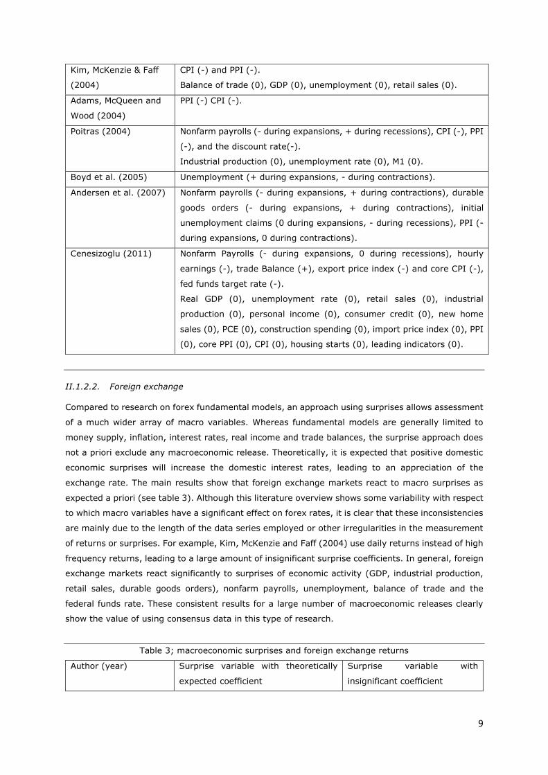
9
Kim, McKenzie & Faff
(2004)
CPI (-) and PPI (-).
Balance of trade (0), GDP (0), unemployment (0), retail sales (0).
Adams, McQueen and
Wood (2004)
PPI (-) CPI (-).
Poitras (2004) Nonfarm payrolls (- during expansions, + during recessions), CPI (-), PPI
(-), and the discount rate(-).
Industrial production (0), unemployment rate (0), M1 (0).
Boyd et al. (2005) Unemployment (+ during expansions, - during contractions).
Andersen et al. (2007) Nonfarm payrolls (- during expansions, + during contractions), durable
goods orders (- during expansions, + during contractions), initial
unemployment claims (0 during expansions, - during recessions), PPI (-
during expansions, 0 during contractions).
Cenesizoglu (2011) Nonfarm Payrolls (- during expansions, 0 during recessions), hourly
earnings (-), trade Balance (+), export price index (-) and core CPI (-),
fed funds target rate (-).
Real GDP (0), unemployment rate (0), retail sales (0), industrial
production (0), personal income (0), consumer credit (0), new home
sales (0), PCE (0), construction spending (0), import price index (0), PPI
(0), core PPI (0), CPI (0), housing starts (0), leading indicators (0).
II.1.2.2. Foreign exchange
Compared to research on forex fundamental models, an approach using surprises allows assessment
of a much wider array of macro variables. Whereas fundamental models are generally limited to
money supply, inflation, interest rates, real income and trade balances, the surprise approach does
not a priori exclude any macroeconomic release. Theoretically, it is expected that positive domestic
economic surprises will increase the domestic interest rates, leading to an appreciation of the
exchange rate. The main results show that foreign exchange markets react to macro surprises as
expected a priori (see table 3). Although this literature overview shows some variability with respect
to which macro variables have a significant effect on forex rates, it is clear that these inconsistencies
are mainly due to the length of the data series employed or other irregularities in the measurement
of returns or surprises. For example, Kim, McKenzie and Faff (2004) use daily returns instead of high
frequency returns, leading to a large amount of insignificant surprise coefficients. In general, foreign
exchange markets react significantly to surprises of economic activity (GDP, industrial production,
retail sales, durable goods orders), nonfarm payrolls, unemployment, balance of trade and the
federal funds rate. These consistent results for a large number of macroeconomic releases clearly
show the value of using consensus data in this type of research.
Table 3; macroeconomic surprises and foreign exchange returns
Author (year) Surprise variable with theoretically
expected coefficient
Surprise variable with
insignificant coefficient

10
Andersen, Bollerslev,
Diebold, and Vega
(2003)
GDP (advance and preliminary),
nonfarm payrolls, retail sales,
industrial production, durable goods
orders, construction spending, factory
orders, trade balance, PPI, CPI,
consumer confidence index, NAPM
index, housing starts, target federal
funds rate, initial unemployment
claims, M1, M2 and M3.
Capacity utilization, personal
income, consumer credit,
personal consumption
expenditures, new home sales
business inventories,
government budget deficit,
index of leading indicators.
Kim, McKenzie, Faff
(2004)
Balance of trade. GDP, unemployment, retail
sales, PPI, CPI.
Andersen, Bollerslev,
Diebold and Vega
(2007)
Nonfarm payrolls, durable goods
orders, initial unemployment claims.
PPI.
Faust, Rogers, Wang,
and Wright, (2007)
Federal funds rate, GDP, initial
unemployment claims, nonfarm
payrolls, retail sales, trade balance
and unemployment
CPI, PPI, housing starts.
II.1.2.3. Fixed income
From a theoretical perspective, it is expected that “good” economic surprises (i.e. macro
announcements indicating a stronger than expected economy) will increase interest rates, and
therefore reduce bond and bill prices. An overview of the macro surprise effect on fixed income
returns (see table 4) largely confirms this theoretical viewpoint; in general surprises denoting “good”
news indeed increase fixed income rates. The variables that generally support this empirical finding
include GDP, industrial production, nonfarm payrolls, initial jobless claims, unemployment, retail
sales, factory orders, durable goods orders, consumer confidence, the NAPM index, housing starts,
money supply, CPI, and PPI. The only macro variables which are consistently categorized as
insignificant are business inventories, the balance of trade and balance of trade proxies.
A priori we don’t expect to see any time-varying effects of macro surprises on interest rates. Only a
few papers report research on whether the state of the economy could influence the macro surprise
– interest rate relationship; McQueen and Roley (1993) and Andersen, Bollerslev, Diebold and Vega
(2007) find constant effects of surprises on interest rates, regardless of the state of the business
cycle. On the other hand, Boyd et al. (2005) find that unemployment surprises have a negative effect
on interest rates in expansions, but no effect during economic contractions.
The papers listed in table 4 report returns of long term bonds as well as short term bills. In general,
all maturities (from 3 month bills up to 30 year bonds) react significantly to surprise in macro
announcements. However, the term structure of US (and foreign) interest rates doesn’t simply move
vertically in response to macroeconomic news; McQueen and Roley (1993) and Faust, Rogers, Wang,
and Wright (2007) show that short and medium term interest rates are more sensitive to macro
surprises than long term rates, or as Faust et al. (2007, p. 1057) put it; “the effect is hump shaped

11
with a maximum effect at about 2 years”. Even though long term rates are less sensitive to macro
surprises, it is clear that, due to their higher duration, prices of long term bond portfolios will react
more strongly than short term bills. This is clearly shown by Balduzzi, Elton, and Green (2001), who
compare prices of 3 month bills, 2 and 10 year notes and 30 year bonds.
It is interesting to note that the effect of US macro surprises reported in table 4 holds for US as well
as EMU fixed income markets; indeed, different authors such as Ehrmann and Fratzscher (2005),
Andersson, Overby and Sebestyen (2009) and Andersen, Bollerslev, Diebold and Vega (2007) find
that Euro area bonds react significantly to US macro surprises, and that this effect is stronger than
for the equivalent euro area surprises. As Ehrmann and Fratzscher (2005, p. 928) put it; “In recent
years certain US macroeconomic news affect euro area money markets and have become good
leading indicators for the euro area”. Similarly, Andersson et al. (2009) find that German government
bond futures react more strongly to US macro surprises compared to German and euro area
announcements. They find that the effect of US releases has become more important during the
period considered (’99-’05).
Finally, it should be noted that two papers in table 4 found a rather high number of insignificant
surprise coefficients; this is notably the case for Kim, McKenzie and Faff (2004) and Ehrmann and
Fratzscher (2005). This is mainly because these two papers use daily return data, whereas other
papers generally use high-frequency returns.
Table 4; macroeconomic surprises and fixed income returns
Author (year) Surprise variables with a theoretically
expected coefficient
Surprise variable with an
insignificant coefficient
McQueen and
Roley (1993)
Industrial production, unemployment,
nonfarm payrolls, PPI, CPI, M1, fed funds
discount rate.
Merchandise trade deficit.
Balduzzi, Elton,
and Green
(2001)
Durable goods orders, housing starts, initial
jobless claims, nonfarm payrolls, PPI, CPI,
consumer confidence, NAPM index, new home
sales, unemployment, retail sales, capacity
utilization, industrial production, factory
orders, M2.
Leading indicators,
merchandise trade balance,
US imports, US exports,
business inventories,
construction spending,
personal consumption,
personal income, treasury
budget, M1, M3.
Hautsch and
Hess (2002)
Nonfarm payrolls, unemployment, hourly
earnings, NAPM index, overall CPI, core CPI,
housing starts, M2, Retail Sales.
Kim, McKenzie,
Faff (2004)
Retail sales, PPI and CPI. Balance of trade, GDP,
unemployment
Boyd et al.
(2005)
Unemployment news in expansions Unemployment news in
contraction

12
Ehrmann and
Fratzscher
(2005)
Feral funds target rate, NAPM index, nonfarm
payrolls, consumer confidence, retail sales.
Industrial production, GDP,
CPI, unemployment rate, PPI,
housing starts, trade balance.
Andersen,
Bollerslev,
Diebold and Vega
(2007)
Durable goods orders, nonfarm payrolls, initial
jobless claims, PPI.
Faust, Rogers,
Wang, and
Wright (2007)
GDP, retail sales, housing starts, initial jobless
claims, unemployment, nonfarm payrolls, PPI,
CPI, trade balance, Federal funds rate.
Andersson,
Overby,
Sebestyen
(2009)
GDP, industrial production, nonfarm payrolls,
initial jobless claims, retail sales, factory
orders, durable goods orders, University of
Michigan consumer sentiment index, Chicago
PMI, consumer confidence, Philadelphia Fed
Business Outlook Survey, ISM non-
manufacturing confidence, CPI, PPI.
Business inventories.
From the discussion above, it is clear that the use of consensus data and the corresponding macro
surprises is a relevant way of searching for the macro variable – asset return relationship. Whereas
previous literature was generally not able to link asset prices to their macro fundamentals, the novel
papers combining consensus data and high frequency returns have provided more consistent findings.
This holds for stock markets, forex as well as bond returns. Andersen, Bollerslev, Diebold and Vega
(2007, p. 251), who search for the effect of macro surprises on different asset classes, conclude; “We
find that news produces conditional mean jumps; hence high-frequency stock, bond and exchange rate
dynamics are linked to fundamentals”.
However, this approach using macro surprises to explain high frequency returns entails some
downsides;
- The interaction or aggregation of macro surprises has hardly been discussed in literature so far.
For example, Andersen et al. (2003, 2007) only consider the joint effect of macro surprises if the
corresponding announcements are released at the same time.
- Macro expectations often show long periods of too optimistic forecasts, followed by long periods
of too pessimistic forecasts (cf. supra). This effect is ignored by the papers listed above.
- High frequency returns provide, per definition, only very limited and short term insight into the
evolution of asset prices. The results from these papers can hardly be used for an asset allocation
or market timing strategy.
Surprise indices, discussed in the next paragraphs, are a novel way of searching for a macro surprise –
asset return relationship, and potentially can surpass some of the shortcomings listed above.

13
II.1.3. Surprise indices
Surprise indices allow to track the performance of economic forecasts by aggregating past
macroeconomic surprises into a comprehensive index. The first surprise indices emerged some 15
years ago, and often have been quoted in popular press2 ever since. The popularity of surprise indices
is also clearly denoted by the large number of banks who have now created their own surprise index.
The best known examples include the Citigroup Economic Surprise index (CESI), Bloomberg
Economic Surprise index, HSBC US activity index, Schroders’ index, and the JP Morgan Economic
Activity Surprise Index (EASI). In a recent press release3, JP Morgan claimed that; “Almost all large
dollar drops in recent years have coincided with phases of pessimism as defined by the EASI, (…)
and trading EASI signals would have delivered annual returns of 8.2%”.
Despite the apparent popularity and usefulness of surprise indices, literature on this type of data is
almost nonexistent. The only noteworthy paper is by Scotti (2012), who compares the US Citigroup
Economic Surprise index with a self-created macro surprise index. In this paper, surprise indices are
used in an ordinary regression to explain foreign exchange returns. Although the R² of these
regressions are rather low (<0,05), the surprise indices are often significant and generally have the
right sign (a positive change in the US surprise index appreciating the US dollar and vice versa).
Because of the apparent lack of literature on surprise indices (except for the work of Scotti, 2012),
these indices will be subsequently discussed further in this thesis. More concretely, investigation will
be carried out as to whether these indices are linked to past asset returns, and whether they can
predict future returns. It will be researched whether it is possible to deduct an asset allocation
strategy from the evolution of a surprise index; specifically, checking whether these indices can be
used for the market timing of bond portfolios with a high duration.
By doing so, this thesis will be different from conventional macro surprise research (cf. infra II.1.2)
because;
- Individual surprises are aggregated into an all-inclusive surprise index. In such a setting,
individual surprises are not of interest anymore; on the contrary, this type of research investigates
whether it is the aggregation of surprises that contains additional information.
- High frequency returns are not used; rather it is assessed whether longer term asset returns
respond to aggregated surprises.
- This thesis is not limited to a descriptive approach; the aim is to look for an effective market
timing strategy.
2 See, for example, Friedman (2012) or Levkovich (2012). 3 JPMorgan, February 7, 2002, JPMorgan introduces the economic activity surprise index, URL; <http://investor.shareholder.com/jpmorganchase/releasedetail.cfm?releaseid=145456>
14
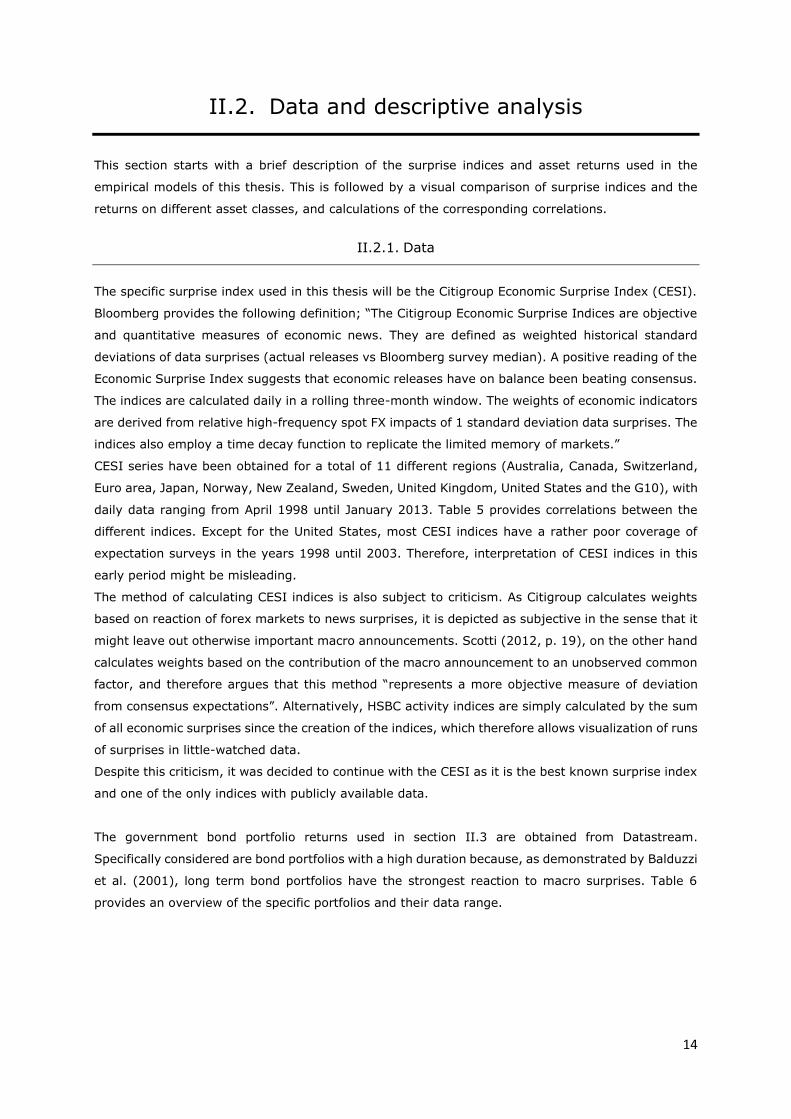
II.2. Data and descriptive analysis
This section starts with a brief description of the surprise indices and asset returns used in the
empirical models of this thesis. This is followed by a visual comparison of surprise indices and the
returns on different asset classes, and calculations of the corresponding correlations.
II.2.1. Data
The specific surprise index used in this thesis will be the Citigroup Economic Surprise Index (CESI).
Bloomberg provides the following definition; “The Citigroup Economic Surprise Indices are objective
and quantitative measures of economic news. They are defined as weighted historical standard
deviations of data surprises (actual releases vs Bloomberg survey median). A positive reading of the
Economic Surprise Index suggests that economic releases have on balance been beating consensus.
The indices are calculated daily in a rolling three-month window. The weights of economic indicators
are derived from relative high-frequency spot FX impacts of 1 standard deviation data surprises. The
indices also employ a time decay function to replicate the limited memory of markets.”
CESI series have been obtained for a total of 11 different regions (Australia, Canada, Switzerland,
Euro area, Japan, Norway, New Zealand, Sweden, United Kingdom, United States and the G10), with
daily data ranging from April 1998 until January 2013. Table 5 provides correlations between the
different indices. Except for the United States, most CESI indices have a rather poor coverage of
expectation surveys in the years 1998 until 2003. Therefore, interpretation of CESI indices in this
early period might be misleading.
The method of calculating CESI indices is also subject to criticism. As Citigroup calculates weights
based on reaction of forex markets to news surprises, it is depicted as subjective in the sense that it
might leave out otherwise important macro announcements. Scotti (2012, p. 19), on the other hand
calculates weights based on the contribution of the macro announcement to an unobserved common
factor, and therefore argues that this method “represents a more objective measure of deviation
from consensus expectations”. Alternatively, HSBC activity indices are simply calculated by the sum
of all economic surprises since the creation of the indices, which therefore allows visualization of runs
of surprises in little-watched data.
Despite this criticism, it was decided to continue with the CESI as it is the best known surprise index
and one of the only indices with publicly available data.
The government bond portfolio returns used in section II.3 are obtained from Datastream.
Specifically considered are bond portfolios with a high duration because, as demonstrated by Balduzzi
et al. (2001), long term bond portfolios have the strongest reaction to macro surprises. Table 6
provides an overview of the specific portfolios and their data range.
15
Table 5; correlations between Citi Economic Surprise Indices
CESI
CAD
CESI
EUR
CESI
G10
CESI
JPY
CESI
NZD
CESI
NOK
CESI
SEK
CESI
CHF
CESI
GBP
CESI
USD
CESI
AUD
CESICAD 1.0000
CESIEUR 0.1180 1.0000
CESIG10 0.2274 0.7241 1.0000
CESIJPY 0.0162 0.0784 0.2287 1.0000
CESINZD 0.1427 0.1001 -0.0078 -0.0615 1.0000
CESINOK -0.0144 -0.1033 -0.0521 -0.1542 -0.0816 1.0000
CESISEK -0.0756 0.1871 0.1472 -0.0787 -0.0827 0.0954 1.0000
CESICHF 0.3122 0.3352 0.3395 0.0703 0.0322 -0.1349 0.0633 1.0000
CESIGBP -0.0803 0.1641 0.3521 0.0093 -0.0448 -0.0259 0.1417 -0.1410 1.0000
CESIUSD 0.1271 0.1873 0.7874 0.0498 -0.1048 0.0197 0.0493 0.17026 0.2862 1.0000
CESIAUD 0.1797 -0.0141 0.1104 -0.0034 0.0054 0.1243 -0.0101 0.0352 0.0795 0.0950 1.0000
Table 6; long term government bond portfolios
Portfolio Datastream
mnemonic Data range
Canada 30 year government bond return
index BMCN30Y(RI) 1/4/’98 – 31/1/’13
EMU 30 year government bond return index BMEM30Y(RI) 1/1/’99 – 31/1/’13
Japan 30 year government bond return index BMJP30Y(RI) 31/12/’99 – 31/1/’13
UK 30 year government bond return index BMUK30Y(RI) 1/4/’98 – 31/1/’13
UK 50 year government bond return index BMUK50Y(RI) 31/5/’05 – 31/1/’13
USA 30 year government bond return index BMUS30Y(RI) 1/4/’98 – 31/1/’13
The return indices are calculated by the formula;
𝑅𝐼𝑡 = 𝑅𝐼𝑡−1 ∗ ∑ (𝑃𝑖,𝑡 + 𝐴𝑖,𝑡 + 𝐶𝑃𝑖,𝑡 + 𝐺𝑖,𝑡) ∗ 𝑁𝑖,𝑡−1𝑖
∑ (𝑃𝑖,𝑡−1 + 𝐴𝑖,𝑡−1 + 𝐶𝑃𝑖,𝑡−1) ∗ 𝑁𝑖,𝑡−1𝑖
Where P is the middle price of the bond, A is the accrued interest, Gi,t is the value of any coupon
payment received from the ith bond at time t since time t-1, N is the nominal value of the amount
outstanding, CP is the value equal to the next coupon payment in the ex-dividend period or 0 outside
the ex-dividend period.
The money market rates used in section II.3 are presented in table 7. The overnight currency
deposits are obtained from Bloomberg, while the Japanese overnight uncollateralized call money rate
is obtained from Datastream.
Other series used in section II.2.2 include the S&P500, Euro Stoxx 50, and USD exchange rates,
which are obtained from Bloomberg. Data ranges from April 1998 up to January 2013. Returns are
generally calculated using past 3 month percentages or natural log differences.

16
Table 7; money market rates
Portfolio Mnemonic Data range
CAD overnight deposit CDDR1T 1/4/’98 – 31/1/’13
EUR overnight deposit EUDR1T 1/1/’99 – 31/1/’13
Japan overnight uncollateralized call money rate JPCALLO(IR) 31/12/’99 – 31/1/’13
GBP overnight deposit BPDR1T 1/4/’98 – 31/1/’13
GBP overnight deposit BPDR1T 31/5/’05 – 31/1/’13
USD overnight deposit USDR1T 1/4/’98 – 31/1/’13
II.2.2. Descriptive analysis
This section provides graphs and correlation tables to show how surprise indices and asset returns
of the USA, as well as foreign markets are related. The discussion starts with stock markets, followed
by foreign exchange , and finally fixed income markets.
II.2.2.1. Stock markets
The figure below presents the USA Citigroup Economic Surprise Index (CESIUSD) together with the
S&P500 3 month % return. This long horizon for S&P returns has been modeled specifically because
the CESI indices are calculated using an aggregate of the past 3 month surprises, too. However,
mind that this definition of the CESI (aggregate of 3 month past surprises) and S&P returns (3 month
past returns) induces a form of autocorrelation; the value of a particular day will be very close to the
value on the previous day.
Drawing S&P500 returns with surprises of other regions (such as the CESI of the G10 or Euro area,
or a difference of these indices - not shown here), does not display a clear fit such as in figure 1. The
relationship between the CESIUSD and S&P500 returns is visibly dependent on the state of the
economy. When the economy is in clear expansion (mid-2004 up to the end of 2007), there is a
negative correlation between surprises and S&P500 returns. Otherwise (mid-1998 up to mid-2004
and 2008 up to now), the correlation is positive.
Figure 2 shows the relationship between the Euro Stoxx 50 and the CESIUSD. Drawing the Euro
Stoxx 50 together with other surprise indices (such as the CESI of the Euro area or other regions –
not shown here) does not display a clear fit such as in figure 2. Again, the correlation between these
two series is clearly dependent on the state of the economy; in the pre-2004 and post-2008 period,
the correlation is clearly positive, whereas in in the period between mid-2004 and the end of 2007,
the correlation turns negative.
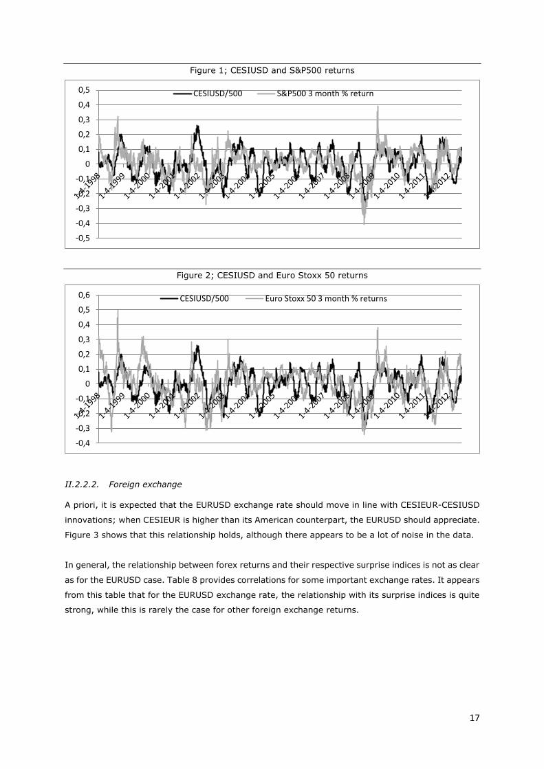
17
Figure 1; CESIUSD and S&P500 returns
Figure 2; CESIUSD and Euro Stoxx 50 returns
II.2.2.2. Foreign exchange
A priori, it is expected that the EURUSD exchange rate should move in line with CESIEUR-CESIUSD
innovations; when CESIEUR is higher than its American counterpart, the EURUSD should appreciate.
Figure 3 shows that this relationship holds, although there appears to be a lot of noise in the data.
In general, the relationship between forex returns and their respective surprise indices is not as clear
as for the EURUSD case. Table 8 provides correlations for some important exchange rates. It appears
from this table that for the EURUSD exchange rate, the relationship with its surprise indices is quite
strong, while this is rarely the case for other foreign exchange returns.
-0,5
-0,4
-0,3
-0,2
-0,1
0
0,1
0,2
0,3
0,4
0,5 CESIUSD/500 S&P500 3 month % return
-0,4
-0,3
-0,2
-0,1
0
0,1
0,2
0,3
0,4
0,5
0,6 CESIUSD/500 Euro Stoxx 50 3 month % returns

18
Figure 3; CESIEUR-CESIUSD and EURUSD returns
Table 8; correlations between 3 month % forex returns and surprise indices
Exchange rate EURUSD USDJPY USDCAD GBPUSD AUDUSD
Surprise indices CESIEUR-CESIUSD
CESIUSD-CESIJPY
CESIUSD-CESICAD
CESIGBP-CESIUSD
CESIAUD-CESIUSD
Correlation 0,2917 0,2203 -0,1099 -0,0276 -0,0474
Exchange rate USDCHF USDSEK NZDUSD USDNOK
Surprise indices CESIUSD-CESICHF
CESIUSD-CESISEK
CESINZD-CESIUSD
CESIUSD-CESINOK
Correlation 0,2111 -0,1112 0,0749 -0,1056
As an illustration, provided is a figure of 3 month USDJPY returns together with the surprise index
CESIUSD-CESIJPY. It appears from this figure that the relationship between the two series is rather
unclear.
Figure 4; CESIUSD-CESIJPY and USDJPY returns
-0,3
-0,25
-0,2
-0,15
-0,1
-0,05
0
0,05
0,1
0,15
0,2 (CESIEUR-CESIUSD)/1000 EURUSD 3 month log return
-200
-150
-100
-50
0
50
100
150
200
-0,25
-0,2
-0,15
-0,1
-0,05
0
0,05
0,1
0,15 USDJPY3 month % return CESIUSD-CESIJPY

19
II.2.2.3. Fixed income
A priori, a strong relation is expected between surprise indices and fixed income returns; positive
surprises should result in higher interest rates and therefore lower prices of bond portfolios. As
previous research (cf. II.1.2.3) already demonstrated a strong effect of macro surprises on interest
rates, it is expected that also surprise indices should have a strong relationship with bond returns.
Figure 5 compares the CESIUSD with the return on a portfolio of 30 year US government bonds;
visibly, the link between these two series is very strong.
Figure 5; CESIUSD and 3 month log returns of a 30 year T bond portfolio
As explained in section II.1.2.3, Euro area bonds have a stronger link with USA surprises compared
to domestic news. Figure 6 therefore compares the returns of 30 year EMU bonds with an index of
USA surprises. Obviously, the relationship is not as good as in figure 5, but it is still clear that the
CESIUSD index can explain a considerable part of the innovations in the 30 year EMU government
bond portfolio. Visibly, the link between the two series has become stronger over time; this has
already been documented by Andersson et al. (2009), who also find that the reaction of German
bond markets to US releases has become more significant during the period 1999-2005.
Figure 6; CESIUSD and 3 month log returns of a 30 year EMU bond portfolio
-0,3
-0,2
-0,1
0
0,1
0,2
0,3
0,4 CESIUSD/500 (inverted) 3 month log return
-0,3
-0,2
-0,1
0
0,1
0,2
0,3
0,4 CESIUSD/500 (inverted) 3 month log return
20
The table below provides a complete overview of the correlations between surprise indices and
returns on the long term government bond portfolios which will be used in section 3.
Table 9; correlations between surprise indices and 3 month % returns of long term government
bonds
Bond portfolio Canada 30Y
EMU 30Y Japan 30Y UK 30Y UK 50Y USA 30Y
Surprise index CESICAD CESIEUR CESIJPY CESIGBP CESIGBP CESIUSD
Correlation -0,1805 -0,2647 -0,3065 -0,0707 -0,0364 -0,4688
Bond portfolio Canada 30Y
EMU 30Y Japan 30Y UK 30Y UK 50Y USA 30Y
Surprise index CESIUSD CESIUSD CESIUSD CESIUSD CESIUSD CESIUSD
Correlation -0,3362 -0,3848 -0,3843 -0,2793 -0,2405 -0,4688
It appears from this table that, as expected, bond portfolio returns have high (absolute) correlations
with surprise indices. It is apparent that these portfolios have consistently higher correlations with
US surprises compared to their respective domestic surprise indices. This finding is in line with
Ehrmann and Fratzscher (2005) and Andersson et al. (2009), who both comment on high spillover
effects from US news on foreign bond markets.
II.2.2.4. Concluding notes
Looking at the three asset classes discussed above, it can be stated that there is overall a clearly
visible relationship between the Citi Economic Surprise Indices and asset returns. Again, this is
evidence that asset returns are linked to macro fundamentals. The CESI has an apparent relationship
with stock indices for different regions. Consistent with other research, it was found that this
relationship is dependent on the state of the economy. The link between foreign exchange rates and
surprise indices is often not that clear, although the correlation between the EURUSD and CESIEUR-
CESIUSD is quite high. This high correlation specifically for the EURUSD is not a coincidence; after
all, this is the most liquid currency pair with the highest volume in the forex market4. Consistent with
the findings of Andersen et al. (2007), it was found that fixed income markets react most strongly
to macroeconomic surprises. Just like previous research, it is shown that interest rates are more
related to the USA surprises than domestic surprise indices.
II.3. Method and results
The previous section has shown that, of all asset classes considered, the fixed income market has
the clearest relationship with surprise indices. Specifically, it was decided to make use of long term
bonds in our models. Although Faust et al. (2007) have shown that long term interest rates have a
4 The Foreign Exchange Committee, October 2012, FX volume survey, URL; <http://www.newyorkfed.org/FXC/volumesurvey/>

21
comparatively small reaction to macro surprises, Balduzzi et al. (2011) reported that the price
reaction of long term bonds, due to their high duration, is relatively bigger compared to shorter
maturities. Therefore, long term bonds should also have the clearest reaction to changes in surprise
indices. In section 3.1, the relationship between high duration government bond portfolios and
surprise indices will be formalized. Section 3.2. will explain how surprise indices can potentially be
used to actually time the fixed income market. To end is the simulation of a market timing strategy
for six different bond portfolios.
II.3.1. Surprise indices and long term government bond returns
Previous literature has already shown a clear effect of macro surprises on high frequency bond
returns (cf. 1.2.3). In line with the descriptive statistics in section 2, the intention is to formally test
whether the effect on bond returns is also significant for macro surprise indices. To this end, we
regress the following equation;
𝑟(𝑡) = 𝛼 + 𝛽𝑟(𝑡 − 1) + 𝛾1∆𝐶𝐸𝑆𝐼𝑈𝑆𝐷(𝑡) + 𝛾2∆𝐶𝐸𝑆𝐼𝐷𝑜𝑚𝑒𝑠𝑡𝑖𝑐(𝑡) + 𝜀(𝑡)
With r(t) the daily return, measured as the first difference of natural logarithms, of a long term
government bond portfolio. This return is regressed on its lagged value, together with the first
difference of the CESIUSD index and, when applicable, the first difference of the domestic CESI
index. We use White heteroscedastic robust errors to account for heterogeneity. In general, no
autocorrelation is found, nor was an important degree of multicollinearity detected. Normality for the
error terms is generally rejected, but does not seem problematic due to the large sample size (>2000
observations). Table 10 shows the results;
Table 10; Regressions of bond returns on surprise indices
Note; numbers in parentheses are t-statistics. *, ** and *** denote significance at a 10%, 5% or
1%, respectively.
R²
Canada 30 years 0.0002*** 0.0477** -0.0001*** -0,00004*** 0.0229
(3.1171)*** (2.3344)** (-6.5786)*** (-3.8958)***
EMU 30 years 0.0002** 0.1288*** -0.0001*** -0,00004*** 0.0281
(2.0879)** (5.9755)*** (-5.6319)*** (-2.9038)***
Japan 30 years 0.0001 0.1167*** -0,00003** -0,00002 0.0155
(1.0730) (4.3276)*** (-1.9622)** (-1.1914)
UK 30 years 0.0002** 0.0715*** -0.0001*** -0,00004*** 0.0163
(2.0585)** (2.9957)*** (-5.3528)*** (-2.9823)***
UK 50 years 0.0002 0.0800** -0.0001*** -0,00006*** 0.0175
(1.0319) (2.3779)** (-3.2647)*** (-2.7211)***
USA 30 years 0.0002* 0.0147 -0.0002*** 0.0251
(1.7391)* (0.6959) (-9.1413)***
22
Whereas previous literature has already shown that bond markets react significantly to macro
surprises, the results in table 10 now also confirm that bond returns are significantly connected to
macro surprise indices. The coefficients 1 and 2 are negative, as a priori expected, and often
significant at the 1% level. Similar to previous literature on macro surprises, R² statistics are quite
low (<0,029).
For all bond portfolios, it appears that the coefficients of the CESIUSD index are bigger (in absolute
value) and more significant than their respective domestic CESI counterparts. Again, this is in line
with the research of Ehrmann and Fratzscher (2005) and Andersson et al. (2009), who both find high
spillover effects from US surprises on foreign bond markets.
II.3.2. Timing government bond portfolios
II.3.2.1. Market timing strategy
Now that the relationship between bond returns and the CESI has been formally established, it could
be asked whether these surprise indices can be used for market timing purposes. The logic behind
the timing strategy is as follows; when the derivative of a CESI index is high, this means that recently
some positive macro news has been published. This is a sign of an economy in expansion, which
should result in higher interest rates, and therefore lower the return on a bond portfolio. As
graphically illustrated in section II.2.2, surprise indices are generally persistent, in the sense that
long periods of rising surprise indices (overly optimistic forecasts) are visible, followed by long periods
of declining surprise indices (overly pessimistic forecasts). This finding is useful for market timing,
as this could mean that a rising surprise index (implying rising interest rates) is a signal to sell long
term bond portfolios in the favor of cash or other money market instruments. This reasoning will be
empirically validated in the next paragraphs.
For this market timing strategy, an investor is modeled who has the choice between investing either
in long term government bonds of one specific country, or overnight money market deposits of the
same currency. The portfolio can be adapted every day. Although government bond returns of 5
different regions are available, the investor will only look at the CESIUSD index (and not the domestic
CESI index). Indeed, section II.2.2. has shown the correlations between USA surprises and
government bond returns to be higher compared to domestic surprises. When the first derivative of
the CESIUSD index is high (low), the investor will invest 100% in overnight currency deposits (a long
term government bond portfolio).
For most government bond portfolios, data is available from 1998 until 2013. This range will be
divided into an in-sample and out-of-sample period. Looking at other research on market timing,
e.g. Resnick & Shoesmith (2002) use an in sample period of 1/4 of the total data range , Rapach et
al. (2005) use an in sample period of 3/5 of the total data range, and Chen (2009) uses an in sample
period of 1/5 of the total data range. In this thesis, an in-sample period of 3 years is chosen compared
to an out-of-sample period of 12 years.
The in-sample period serves for two purposes. First of all, a precise definition of “derivative” will be
determined; the derivative of a surprise index can be measured as difference in levels between two
subsequent days, 3 subsequent days, 10 subsequent days etc. It is clear that, when a derivative is

23
defined as a short term (e.g. 2 day) difference of the level of a surprise index, the investor will
rebalance his portfolio more frequently compared to when the derivative is defined as a long term
(e.g. 20 day) difference in the level of the CESI. The in-sample period will determine the definition
of “derivative” which is the most profitable for market timing. Second, a threshold has to be
determined for when a derivative is categorized is “high”. In the in-sample period, the percentile of
derivatives will be calculated for which the corresponding threshold leads to the highest profitability
for our market timing strategy. These definitions of the derivative and threshold level are continued
throughout the remaining years of the out-of-sample period.
Afterwards, the profitability of this market timing strategy is compared with a buy and hold of the
corresponding long term government bond portfolio and overnight currency deposits.
In order to assess whether the market timing ability of our model is statistically significant, the
Pesaran and Timmermann nonparametric test is conducted. As Pesaran and Timmermann (1992, p.
461) state, this test is particularly useful when “the focus of the analysis is on the correct prediction
of the direction of change in the variable under consideration”, as is the case in this model. This test
does not a priori restrict the distribution of variables, and holds as long as the government bond
portfolio returns and the first derivative of the CESIUSD are symmetrically distributed around 0.
Another advantage of this test is that, contrary to risk based measures such as the Sharpe ratio,
Jensen’s alpha or the two beta model of Hendriksson and Merton, the nonparametric test of Pesaran
and Timmermann does not require the definition of a market and risk free portfolio. This test statistic
is defined as follows;
𝑆 =𝑝 − 𝑝 ∗
√𝜎𝑝2 − 𝜎𝑝∗
2 ~𝑁(0,1)
Where p is the proportion of times that the sign of yt is predicted correctly; p* = pypx + (1-py)(1-px);
py = Pr(yt>0); px = Pr(xt>0); s2p = n-1p*(1-p*); s2
p* = n-1(2py-1)2px(1-px) + n-1(2px-1)2py(1-py) +
4n-2pypx(1-py)(1-px); xt is the CESIUSD, yt is the daily return of a long term government bond
portfolio minus the overnight rate on a currency deposit.
Lastly, transaction costs must be accounted for. As it is not clear what the average cost would be of
buying or selling portfolios of government bonds, the number of transactions are simply counted
over the period under consideration and a theoretical transaction cost (in % of total portfolio value)
that would make the return of our market timing strategy equal to the bond benchmark is calculated.
II.3.2.2. Market timing results
The results of the market timing strategy are presented in table 11. For 5 out of 6 bond portfolios,
the out-of-sample return of the market timing strategy clearly outperforms the respective
benchmarks. Likewise, the Peseran and Timmermann test is significant at a 5% level for all portfolios.
Keep in mind that all six of the investment strategies are based on the CESIUSD Index. From that
perspective, it is remarkable that this strategy works equally well for US government bonds as well
as most foreign bond portfolios. Market timing does not seem to work for 30 year Canadian
government bonds, although the Pesaran Timmerman statistic is still significant (p-value of 0,0342).
The disappointing out of sample return of Canadian government bonds might be due to their
relatively low volatility. After all, it is more difficult to apply a market timing model to a bond portfolio
with nearly continuously rising prices, compared to a region with much more volatile bond returns.
Table 9 therefore also presents the volatility of the different bond portfolios, measured as the
24
standard deviation of weekly natural log returns. It clearly appears from this table that the portfolio
of 30 year Canadian government bonds is the least volatile.
The yearly returns presented in table 11 don’t take into account transaction costs. The last row of
table 11 therefore shows the theoretical transaction cost (in % of the portfolio value) that would
make the return of our market timing strategy equal to the bond benchmark. These transaction costs
are often quite low (0,086% or smaller), which casts doubt on the ability of this market timing
strategy to yield above benchmark returns in the real world.
A consistent finding emerges from the table below; for most bond portfolios, 5 and 6 day CESIUSD
derivatives appear to provide the best trading strategies. The market timing strategy for US T-bonds
seems to diverge from other bond portfolios with an optimal strategy for 25 day CESIUSD derivatives;
however, keep in mind that this derivative is chosen based on a rather short in-sample period of
about three years. Over the full sample (15 years), a five day strategy seems optimal, anyway.
An important cautionary note is necessary when measuring derivatives over such a short 5 day or 6
day interval; not only will a short interval entail considerable transaction costs, but also such a short
time period will only contain one or two macro releases. This entails that this market timing method
is not very different from conventional research which looks at the effect of a single macro surprise
on asset returns. As an illustration, appendix 1 graphically presents out of sample returns for different
derivative definitions. This is shown for the 70th and 75th percentile strategies for all of the six bond
portfolios. It appears from these figures that, in general, 5 day derivatives are associated with a peak
in out of sample return, while strategies based on longer derivatives are unprofitable.
II.3.2.3. An alternative strategy based on domestic surprise index derivatives
Previous academic literature has shown that fixed income markets react more to US macro surprises
compared to domestic macro events (cf. infra II.1.2.3). This was corroborated by presenting the
correlations between surprise indices and government bond returns (cf. infra II.2.2.3). Similarly, the
market timing strategy shown in the previous paragraph, although based solely on the CESIUSD,
worked equally well for US government bonds as well as foreign bond portfolios. Nevertheless, it
might still be interesting to reproduce a market timing strategy for foreign government bonds by
simultaneously taking into account domestic surprise indices.
The method for this timing strategy is thus similar to the one presented in II.3.2.1. The same
government bond portfolios are used and the same distinction between in sample and out-of-sample
periods remains. However, now the CESIUSD and the domestic surprise index are considered
simultaneously; the investor will buy government bonds once the CESIUSD and the domestic surprise
index derivatives fall below a certain level. This level is determined as the percentile of US and
domestic surprise index derivatives which maximizes profits in the in sample period. All other details
of this market timing strategy are similar to II.3.2.1.
The results of this timing strategy are presented in appendix 2. It appears that in sample as well as
out-of-sample returns are systematically lower compared to the a market timing strategy based
solely on the CESIUSD. Similarly, the Pesaran and Timmermann test statistics are less significant
compared to the p-values presented in table 11. Again, this confirms the finding that bond markets
react more to US macro news compared to domestic macro surprises.
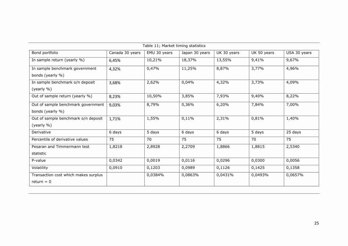
25
Table 11; Market timing statistics
Bond portfolio Canada 30 years EMU 30 years Japan 30 years UK 30 years UK 50 years USA 30 years
In sample return (yearly %) 6,45% 10,21% 18,37% 13,55% 9,41% 9,67%
In sample benchmark government
bonds (yearly %)
4,32% 0,47% 11,25% 8,87% 3,77% 4,96%
In sample benchmark o/n deposit
(yearly %)
3,68% 2,62% 0,04% 4,32% 3,73% 4,09%
Out of sample return (yearly %) 8,23% 10,50% 3,85% 7,93% 9,40% 8,22%
Out of sample benchmark government
bonds (yearly %)
9,03% 8,79% 0,36% 6,20% 7,84% 7,00%
Out of sample benchmark o/n deposit
(yearly %)
1,71% 1,55% 0,11% 2,31% 0,81% 1,40%
Derivative 6 days 5 days 6 days 6 days 5 days 25 days
Percentile of derivative values 75 70 75 75 70 75
Pesaran and Timmermann test
statistic
1,8218 2,8928 2,2709 1,8866 1,8815 2,5340
P-value 0,0342 0,0019 0,0116 0,0296 0,0300 0,0056
Volatility 0,0910 0,1203 0,0989 0,1126 0,1425 0,1358
Transaction cost which makes surplus
return = 0
0,0384% 0,0863% 0,0431% 0,0493% 0,0657%

26
II.3.2.4. An alternative strategy based on surprise index levels
An interesting finding emerges when looking at the CESI plots presented in II.2.2; CESI series appear
to be mean reverting. Over the past 15 years, CESI indices appear to fluctuate around 0, with long
periods of positive surprises followed by long periods of negative surprises. Therefore, if a CESI index
is at an extreme level, two things may happen; either forecasters will adapt their estimates in the
right direction, either subsequent macro releases will be more in line with their respective forecasts.
In the two cases, the CESI will go back to 0. More formally, unit root tests (see appendix 3) confirm
that surprise indices are mean reverting.
It could therefore be asked whether extreme levels of surprise indices provide information to trade.
E.g. when the CESIUSD is at a high level, this could mean that future surprises will be lower (as the
CESI always mean reverts), that interest rates will decline, and that therefore the value of long term
government bond portfolios will increase.
Thus, it could be interesting to check whether the level of the CESI can be used in a bond timing
strategy. As a preliminary analysis, the levels of the CESIUSD are divided into different “hurdles” or
percentiles. Subsequently, the corresponding mean future government bond returns are calculated.
These future bond returns are defined as the percentage change over a horizon of 2 weeks and 1, 2,
3 and 6 months. Appendix 4 provides the results. Contrary to intuition, these government bond
portfolio sorts don’t show any meaningful pattern. The same sorts were also conducted for domestic
surprise indices, which again showed no clear results. Therefore, we conclude that the level of the
CESI is not useful for a government bond timing strategy.
II.4. Conclusion
Macro consensus data have gained considerable attention in recent research on the link between
macro surprises and asset returns. The literature overview in section II.1 shows that previous
research using conventional fundamental models and levels of macro variables has not been able to
present stylized facts on the macro variable – asset return relationship. Research using macro
surprises, on the other hand, has obtained some consistent and significant results; foreign exchange
markets, for example, appear to have a strong link with a wide range of macro surprises, while
previous fundamental models weren’t able to produce any consistent results.
Literature on macro surprises has largely ignored the interaction between different surprises. Hence,
this thesis applied macro surprise indices to have a new way of dealing with the macro surprise -
asset return relationship. The descriptive analysis in section II.2 shows that stock returns, forex rates
and bond returns have a clear relationship with these surprise indices.
In section II.3, a market timing strategy is proposed, based on the first derivative of the CESIUSD
index. Results show that, before taking into account transaction costs, this strategy achieves high
excess returns for multiple long term government bond portfolios. These market timing returns are,
however, quite tentative because of the short time frame applied, the short term definition of
derivative (i.e. a 5 or 6 day difference) and because it is unlikely that this strategy yield high returns

27
after taking into account transaction fees. Related government bond timing models based on
domestic surprise index derivatives or levels of surprise indices appear to be unprofitable. In any
case, the market timing returns presented in II.3.2.2 demonstrate that surprise indices have the
potential of being used for asset allocation purposes.
Because surprise indices have been overlooked in current literature up until now, there are many
possibilities for further research. A more formal (descriptive) analysis of the relationship between
surprise indices and asset returns could be useful. Market timing models for other asset classes such
as stock markets and foreign exchange could be interesting, in which it would be challenging to
model state dependent returns. It is clear that many avenues for research on surprise indices are
possible, and that this research could have interesting applications for asset allocation and the macro
variable - asset return relationship.

28
III. DISPERSION & CONSENSUS DATA
III.1. Current literature
This section provides an overview of literature on the dispersion of consensus data and asset returns.
We start by looking at the dispersion of earnings estimates (i.e. micro consensus data), of which
previous empirical research found a clear link with the cross section of stock market returns. Past
literature on the dispersion of macro consensus data is, however, less developed. Empirical studies
on macro dispersion are generally limited to explaining forecast dispersion using other macro factors,
or searching for a link between this forecast dispersion and the variance in asset returns. There also
exists a large set of theoretical models on dispersion, which have however largely remained without
empirical validation. The next paragraphs go deeper into these strands of literature, and give a basis
for building an asset allocation strategy.
III.1.1. Dispersion of micro consensus data
III.1.1.1. Basic empirical research on the micro dispersion – stock return relationship
Ackert and Athanassakos (1997) are among the first to explore the effect of earnings estimate
dispersion on stock returns. They divide a sample of US stocks into different quartiles according to
the standard deviation of earnings estimates and calculate the “overoptimism” (i.e. the difference
between earnings releases and the preceding estimates) for each quartile. A positive relation between
over optimism and uncertainty is found, with little or no optimism for low uncertainty stocks.
Subsequently, average 20 month (excess) returns are calculated for each quartile, where significantly
higher returns are found for low dispersion stocks. This paper finds an annual compounded return
difference between high and low dispersion stocks of 11,35%.
The results of this paper have been confirmed numerous times in subsequent research. Diether,
Malloy and Scherbina (2002), for example, show that going long on low dispersion stocks and short
on high dispersion stocks, generates a 9,5% annual return. They sort this dispersion effect on size,
momentum and book-to-market (BTM) factors, and show that the effect is strongest for small stocks
and shares that have performed poorly over the previous year. They run a series of Fama and
MacBeth (1973) yearly cross sectional regressions and show that the dispersion effect cannot be
explained by a traditional risk framework. They show that the returns are more or less robust to
different specifications in portfolio formations, holding periods, earnings forecasts and sub-periods,
although the return differential is somewhat lower in the 90’s compared to the 80’s.
Hintikka (2008) confirms the findings of Diether et al. (2002) by using data of 7 European countries.
Gharghoria, Seeb and Veeraraghavanc (2011) find similar effects for the Australian stock market.
Ang and Ciccone (2001) again confirm for US stocks that low dispersion portfolios outperform high
dispersion shares. They find that this result cannot be explained by momentum, liquidity, industry,
or traditional risk measures.
Berkman et al. (2009) also find a significant effect of differences of opinion on stock returns. They
use 5 different measures for difference of opinion, including dispersion of earnings forecasts. Other

29
measures such as historical income volatility, stock return volatility, firm age and average daily
turnover often provide even higher return differentials. They use Fama and MacBeth (1973)
regressions to show that this return differential is higher for stocks that are difficult to sell short.
These results are robust after controlling for size, BTM, momentum, leverage, and volume around
earnings announcements.
Dische (2002) shows that the results of dispersion strategy can be improved by simultaneously
sorting the portfolios for an earnings momentum effect. Buying low dispersion shares with positive
earnings revisions and simultaneously shorting high dispersion shares with negative earnings
revisions yields a monthly return of 1,48%. This effect is robust for different sub-periods (‘87–‘91,
‘91–‘95 and ‘95–’00), although the dispersion effect declines over time.
Chahine (2004) specifically looks for an effect of dispersion at earnings announcement days, and
finds that the excess return on the announcement day is negatively related to forecast dispersion
after the preannouncement of earnings.
III.1.1.2. Theories explaining the micro dispersion – stock return relationship
The papers above thus present common findings that a high dispersion in earnings estimates leads
to lower future returns. This is rather surprising, as intuitively, one would expect high dispersion in
micro consensus data to be a proxy for risk, which should lead, on average, to higher returns. One
common explanation for this counterintuitive finding, advocated by a.o. Ackert and Athanassakos
(1997) and Diether et al. (2002), is based on analysts’ behavior. It is a well-known phenomenon
that sell-side analysts have incentives to issue optimistic recommendations. These incentives are
connected to maintaining good relations with client firms and supporting brokerage commissions.
When the dispersion in earnings forecasts is low, a sell-side analyst may opt not to stand out of the
crowd and therefore issue a forecast that is not overly optimistic. However, if a large variation in
forecasts exists, analysts face less problems to act on their incentives to issue an optimistic estimate.
This in turn leads to overvaluation of high dispersion stocks, which inevitably entails poor future
returns when the actual earnings announcements are below expectations.
Another explanation, advocated by a.o. Hintikka (2008) and Gharghoria et al. (2011) is based on the
theory of Miller (1977). In this setting, dispersion in micro consensus estimates are seen as a proxy
for differences of opinion among stock market participants. The theory of Miller then states that,
whenever investors have differing opinions of asset valuations, pricing of these assets will reflect the
view of more optimistic participants if this stock market is characterized by restricted short selling.
This optimistic view thus leads to overvaluations, and therefore low future returns.
The framework of Miller (1977) is often seen as valid explanation, as the research previously
mentioned in this chapter consistently finds that the high dispersion stock portfolio is responsible for
the bulk of the return differential. As it is the high dispersion portfolio that needs to be shorted,
restricted short selling indeed could entail that pricing of this specific portfolio is too high. Also, it is
often documented that the return differential is more significant for small stocks, or more in general,
stocks that are difficult to sell short (see e.g. Diether et al., 2002, or Berkman et al., 2009). Again,
this is consistent with the optimism framework of Miller.
Johnson (2004), on the other hand, provides a theoretical framework which can explain the returns
differentials mentioned above, without presuming any irrationality, frictions, or anomalous analyst
behavior. Johnson constructs a theoretical model for the risk premium of levered firms, based on
30
elementary options pricing. Under the hypothesis that dispersion in a proxy for idiosyncratic risk, it
is shown that dispersion will lower expected returns. This pricing model also states that the strength
of the dispersion – expected return relationship should increase with leverage. This is empirically
validated using Fama-MacBetch cross-sectional regressions.
III.1.1.3. Related empirical research
An interesting variation to the research explained above is the work of Zhang (2006). He also finds
a negative, though insignificant, relation between dispersion of earnings forecasts and future stock
returns. Additionally, Zhang researches whether uncertainty (defined as standard deviation of
earnings forecasts) has an influence on momentum profits (defined as earnings momentum or price
momentum). It is shown that greater uncertainty leads to more significant momentum returns. These
results are also found when abnormal returns are defined as the intercept of a four factor model, and
remain valid for different sub-periods, although the returns decline for larger lags in portfolio
formations. A trading strategy which shorts low momentum, high dispersion stocks and buys high
momentum, high dispersion stocks creates monthly profits of 2,30%. These results are consistent
for other measures of micro uncertainty, such as firm size, firm age, analyst coverage, return
volatility, and cash flow volatility. Zhang therefore suggests that uncertainty postpones the flow of
information into stock prices. These findings are corroborated by Verardo (2009), who also looks for
the effect of micro dispersion on price momentum. Again, it is found that higher dispersion of earnings
estimates leads to larger momentum profits. These findings are robust after controlling for size,
book-to-market, analyst coverage (as a proxy for information diffusion) and idiosyncratic volatility.
However, not all papers on micro dispersion lead to the finding that high dispersion stocks have
consistently lower future returns. Leippold and Lohre (2012), for example, show that this micro
dispersion effect is not consistent for different time frames. As a matter of fact, they do find that
high dispersion portfolios lead to lower future returns, but they show the bulk of this return
differential originates in a narrow time frame of three years around the technology bubble. Therefore,
they conclude that the dispersion effect cannot be used as a long term asset allocation strategy.
Doukas, Kim and Pantzalis (2004) obtain results in contradiction to the conventional micro dispersion
– stock return relationship. They test whether dispersion of analysts’ earnings estimates can explain
the return differential between value and growth stocks. By dividing stocks into quintiles according
to their BTM ratio and calculating the corresponding earnings forecast dispersions, they show that
value stocks have a higher earnings forecasts dispersion compared to growth portfolios. Hence, in
this setting, higher dispersion is actually a proxy for higher risk. This is corroborated by adding a
micro dispersion variable to a Fama and French (1993) three factor model.
Dispersion in earnings forecasts has also been a topic for asset classes other than shares. Güntay
and Hackbarth (2010), for example, look for an effect of earnings dispersion on corporate bond
returns. They show that high dispersion firms have on average higher credit spreads, and that
changes in the level of dispersion can significantly predict changes in these credit spreads. Thus, for
the corporate bond market, dispersion is a proxy for cash flow uncertainty (i.e. risk), in contradiction
with the theory of Miller (1977). This, in turn, is explained by the limited short-sale constraints of
bond markets.

31
III.1.2. Dispersion of macro consensus data
The previous section has shown that a wide range in literature finds a consistent, negative
relationship between micro dispersion and future stock returns. Literature on macro dispersion,
however, is less developed. In the next paragraphs, it is discussed how to measure macro dispersion.
Subsequently, an overview of related empirical research is given.
III.1.2.1. Measures of macro uncertainty
Macro uncertainty has previously been identified using macroeconomic consensus data, stock return
volatility (e.g. the VIX index), news measures, and economic policy uncertainty (e.g. Baker, Bloom
and Davis, 2012). In this thesis, the focus is on the dispersion in macroeconomic consensus data as
a proxy for uncertainty.
Several authors such as Zarnowitz and Lambros (1987), Giordani and Soderlind (2003), and Bowles
et al. (2007) have compared different measures of macro uncertainty and commented on their
usefulness for different purposes. The main measures of macro uncertainty include (1) the dispersion
across forecasters, (2) average standard deviation of individual distributions, (3) the standard
deviation of the aggregate distribution, (4) uncertainty measures based on surprise indices, and (5)
measures based on forecasting errors or historical volatility.
1. The standard deviation (variance) of point estimates is also commonly referred to as the
disagreement among forecasters. The measure is easy to compute and even directly available on
services such as Bloomberg and the SPF of the Philadelphia FED. However, disagreement might
be related to the number of forecasters, and is also problematic when forecasters are highly
uncertain about the economy, but nevertheless agree with each other on the most likely outcome
(see figure 7a). In that case, the standard deviation of these point forecasters would be very
small, although the overall level of uncertainty has peaked. Giordani and Soderlind (2003)
calculate disagreement as half the distance between the 16th and 84th percentile of point forecasts;
this is a robust measure of dispersion, whereas the conventional standard deviation is more
sensitive to outliers. They find that this robust measure, for Philadelphia SPF data, has a high
correlation with other, more complicated measures of uncertainty, and is therefore a valid
measure of uncertainty. These findings are corroborated by Zarnowitz and Lambros (1987) for a
shorter timeframe of the Philadelphia SPF; their reported correlations between disagreement and
individual uncertainty measures are generally positive and significant. They do warn that
disagreement might overstate the variations in uncertainty, as its fluctuations are far higher than
what should be expected from economic variables (GDP growth, inflation), characterized by
resilience and gradual adjustments.
2. The average standard deviation (variance) of individual distributions is an interesting measure
because it captures the uncertainty of representative agents. However, because this dispersion
measure doesn’t take into account the disagreement across individuals, it is possible that that
forecasters report the same individual uncertainty from one period to another, but disagree among
each other about the mean estimate (see figure 7b). In such a case, simply taking the average
standard deviation of individual distributions might not capture the overall uncertainty of
32
forecasters. Nevertheless, Giordani and Soderlind (2003) see this individual uncertainty as a valid
benchmark for comparison and show that also this measure has a high correlation with the
standard deviation of the aggregate distribution of forecasters and other measures of dispersion.
Likewise, Zarnowitz and Lambros (1987) note that this dispersion measure is overall a good
approximation for the overall level of uncertainty and the variation in uncertainty.
3. The standard deviation (variance) of the aggregate distribution, or aggregate uncertainty, takes
into account both the disagreement and uncertainty of individual forecasters. It can be shown
that the variance of the aggregate distribution is equal to the sum of the average variance of the
individual distributions (=individual uncertainty) and the variance of point estimates
(=disagreement). Because this measure takes into account the two previous dispersion measures,
it could be seen as an encompassing uncertainty measure. It is of particular interest as it is often
shown in empirical literature (e.g. Giordani and Soderlind, 2003, 2006) that individual forecasters
are overconfident about their own estimates, and therefore underestimate uncertainty.
4. Scotti (2012, p.3) recently proposed a new measure of uncertainty, based on consensus data,
calculated as the root of a weighted average of squared surprises. The author argues that;
“Forecast disagreement measures divergence of opinions among forecasters rather than just the
underlying uncertainty about the economy […] My uncertainty measure is a cleaner measure of
the uncertainty regarding the current state of the economy and is available daily.”
Figure 7; different measures of dispersion.
When comparing the first three measures described above, Giordani and Soderlind (2003) find that,
for inflation expectations extracted from the Philadelphia SPF, all three dispersion measures have
high correlations and are generally equally volatile. They therefore conclude that, disagreement, by
far the easiest dispersion metric to compute, is, in their setting a valid measure for uncertainty.
Bowles et al. (2007), on the other hand, compare dispersion measures for inflation, unemployment
and GDP growth from the ECB Survey of Professional Forecasters. They claim that standard deviation
of the aggregate distribution, contrary to disagreement or individual volatility, is the most valid
measure as it corresponds broadly to the historical volatility of the actual data series. However, most
measures of dispersion, including the standard deviation of the aggregate distribution, were
remarkably stable during the recession period centered around 2001. Bowles et al. therefore argue
that these ECB dispersion measures are inconsistent because they haven’t been able to accurately
assess the risks associated with economic downturn.
(a) low disagreement, high individual uncertainty (b) high disagreement, low individual uncertainty

33
Giordani and Soderlind (2003) also compare the three dispersion measures described above with
time series measures of uncertainty. They use the standard deviation of forecast errors from different
models as proxies for uncertainty. Their employed models include a VAR with homoscedastic errors,
a standard GARCH model and an asymmetric GARCH. The authors refute the use of these time series
measures as a proxy for uncertainty because of the low correlations with other dispersion measures
and their inability to account for structural breaks (e.g. a change in inflation rate targets). These
findings are corroborated by Lahiri and Liu (2010), who specifically finds that ARCH estimates tend
to diverge significantly from survey estimates of uncertainty during periods of regime change or
structural break. Arnold and Vrugt (2008) also discuss time series measures of uncertainty from a
theoretical viewpoint; they also refute the use of these time series measures because “uncertainty”
should be an ex ante measure, whereas time series models are backward looking. Neither is there
agreement on a universal time-series model to be used in this context. Finally, as stressed by the
Arnold and Vrugt, time-series volatility just measures one particular ex post realization of a macro
variation out of many ex ante possibilities. It might thus be that ex ante considerable uncertainty
exists about the innovations of macroeconomic factors, whilst this is not necessarily captured by time
series models.
Lahiri and Sheng (2010) also provide interesting insights on the relationship between different
measures of macro uncertainty. They deconstruct the average variance of individual distributions
into disagreement among forecasters, added to the perceived variance of future cumulated shocks.
Therefore, in this setting, the validity of disagreement as a measure for uncertainty is dependent on
the stability of the macroeconomic setting and the length of the forecast horizon. These assumptions
are empirically verified using the Philadelphia FED SPF; disagreement appears to be a reliable proxy
for periods with low volatility of aggregate shocks and short forecast horizons.
Lahiri and Sheng also show that the squared error of consensus estimates is not a good proxy for
variance of future aggregate shocks; augmenting disagreement with the squared error of forecasts
actually performs worse as a measure of uncertainty than disagreement alone. This casts doubt on
the validity of the uncertainty measure proposed by Scotti (2012), who also merely uses a weighted
average of squared surprise as an uncertainty measure.
III.1.2.2. Macro dispersion and asset volatility
The previous section has shown what measures of dispersion in macroeconomic consensus data can
be used as valid proxies for uncertainty. In the next paragraphs, these measures are used in empirical
research on asset volatility.
Whereas previous empirical research on asset volatility has mainly used time series based measures
for uncertainty, Arnold and Vrugt (2008) were among the first to use disagreement as a macro
uncertainty measure in this setting. Their paper includes several interesting findings; firstly, they
calculate a disagreement measure for ten macro variables from the Philadelphia SPF and find that all
of these dispersion measures are significantly higher during NBER defined recessions. Also, it appears
that the disagreement is highly correlated among these different variables, which leads the authors
to conclude that this uncertainty measure is able to capture moments of general economic unease

34
relatively well. Next, by simply regressing S&P500 volatility on the disagreement for different
variables, they show that a large part of these disagreement coefficients are significant, thus
uncertainty about future macroeconomic variables provides information on stock market volatility.
The authors do warn that, starting from 1997, this relationship becomes insignificant, consistent with
other papers who found the structural break in asset volatility around this period, possible caused by
the dotcom bubble. Subsequently, a VAR model is estimated to look for granger causality between
S&P500 volatility and disagreement for different macro variables; results show that five out of ten
disagreement measures have significant predictive power. All the above tests were also conducted
for times series measures of macroeconomic uncertainty, which, compared to disagreement,
generally show a very limited or no relationship with asset volatility.
Glasbeek and Ivo (2011) mainly confirm the aforementioned findings using SPF data of the ECB. The
authors also use disagreement as a measure for macroeconomic uncertainty. Glansbeek and Ivo
conduct an ordinary regression to search for a link between asset volatility and macro uncertainty,
and just like Arnold and Vrugt, they find a significant positive relationship between stock market
volatility and disagreement on different macro variables (real GDP, unemployment and inflation). In
addition, they find that bond market volatility is mainly affected by disagreement on inflation. Finally,
the authors also report on long-run cointegration relationships between stock and bond market
volatilities and disagreement on all three macroeconomic uncertainties (real GDP, inflation, and
unemployment).
III.1.2.3. Macro dispersion and the levels of other macro variables
The two previous sections compared different measures of macro uncertainty and searched for a link
with asset volatility. Interesting questions remain whether macro uncertainty is linked with the state
of the economy, and whether this uncertainty is linked to the level of other macro variables.
Dopke and Fritsche (2006), for example, use ordinary regressions to search for a relationship
between recession periods and disagreement on GDP growth and inflation in Germany. Their results
show that disagreement on GDP growth is significantly larger before and during recessions, while
disagreement is actually lower during early upturns of the economy. Therefore, this finding is broadly
consistent with Arnold and Vrugt (2008). With respect to disagreement on inflation, however, Dopke
and Fritsche find no, or only a very weak positive relationship with recession periods. These differing
results are explained by stating that forecasters might frequently disagree on the current length of
a business cycle, whereas the state of this cycle might not be a good indicator for inflationary
pressures.
D’Amico and Orphanides (2008) use the Philadelphia SPF to search for a link between inflation
uncertainty measures and term premia. They calculate correlations between mean forecasts,
disagreement, average individual uncertainty and 2, 5 and 10 year term premia. All of these premia
have positive correlation coefficients with mean forecasts of inflation (>0,31) as well as with average
individual uncertainty (>0,62), and disagreement (>0,23). These findings are corroborated by
regressing the term premia on each of the previous inflation measures separately. Again, the
relationship is strongest for the average individual uncertainty (R² of 0,38), compared to mean
forecasts of inflation (R² of 0,16) or disagreement (R² of 0,13).
35
D’amico and Orphanides also visually compare series of disagreement and average individual
uncertainty with the level of inflation. They find that level of inflation clearly moves together with
these two dispersion measures. Correlation coefficients confirm these findings; a coefficient of 0,68
is found between the mean inflation forecast and the disagreement on inflation, while this coefficient
is slightly lower for the dispersion of individual distributions.
Mankiw, Reis, Wolfers (2004) corroborate the findings of D’amico and Orphanides and show through
a visual analysis and several regressions that disagreement on inflation forecasts is linked to the
level and change in inflation. On the other hand, the authors find no relationship between
disagreement and the output gap.
Capistran and Timmermann (2009) provide a theoretical framework for the fact that disagreement
in inflation forecasts varies with the level and variance of inflation. Their theoretical model is based
on asymmetric loss (i.e. the cost of over- or underpricing inflation might be uneven), differences in
forecasters’ loss functions, and a constant loss term (i.e. a constant tendency to over- or underpredict
inflation). They empirically validate their model with Philadelphia SPF data, and find evidence for
asymmetric loss, different loss functions and a constant loss term. They find that inflation forecasts
are indeed dependent on the level and conditional variance of current inflation.
III.1.3. Pricing models and the dispersion – asset return relationship
Section 1.1 listed numerous papers which have found a negative relationship between stock returns
and micro dispersion. These empirical findings were shown to be consistent with the framework of
Miller (1977) and the option based pricing theory of Johnson (2004). Besides these two theories on
micro dispersion, there are a large number of other theoretical models available that deal with the
effect of (macro) dispersion on asset returns. These theoretical asset pricing models often have a
basis of aggregate consumption and rely heavily on mathematical deductions. However, a large part
of these models has not been empirically validated yet.
Varian (1985), for example, finds that in an Arrow-Debreu equilibrium, asset prices depend solely on
aggregate consumption and the agent’s subjective probability distributions. For relative risk averse
utility functions, equilibrium asset prices are found to decrease when dispersion of opinion increases.
Soderlind (2006) again considers an Arrow-Debreu equilibrium but deducts a different model
compared to the one of Varian (1985). Soderlind’s modes suggests that the equity premium is
approximately γσ2+δ2, where γ is the risk aversion coefficient, σ2 denotes the variance of an
investor’s individual beliefs on future output, and δ is the disagreement among investors on output
estimates. The implied variance of a stock option is approximately equal to the equity premium
divided by γ. Therefore, the uncertainty of a representative investor equals σ²+δ²/γ. Soderlind thus
states that, if the coefficient of risk aversion is not too small, disagreement will not be very significant
for asset pricing. This effect is amplified by empirical findings from Philadelphia SPF data, which show
that individual uncertainty (σ²) is more than twice as large as disagreement (δ²).
Anderson, Ghysels and Juergens (2009) suggest a very specific definition of uncertainty; they extract
expectations on aggregate profits from the Philadelphia SPF and use these to calculate expected
returns for each forecaster using the Gordon-Shapiro model. The variance across forecasters in these
expected returns is used to proxy for uncertainty. Anderson, Ghysels and Juergens subsequently
deduct a theoretical model, based on Merton (1973), which states that both risk (i.e. the volatility of
36
an asset) and uncertainty (i.e. the variance of expected returns across forecasters) carry a positive
premium. Formally, their model states for the aggregate stock market that;
Etret+1=γVt+θMt
With ret+1 the quarterly excess returns of the stock market over a risk-free bond between t and t+1; Vt
the variance of the market and Mt the uncertainty of the market.
They deduct for an individual stock k;
Etrkt+1=βvkγVt+βukθMt
With βvk and βuk could be seen as regression coefficients of respectively the risk in asset k on market
risk and of the uncertainty in asset k on market uncertainty.
They empirically validate their model and show that in the equation for aggregate excess stock
market returns, θ is highly significant. In addition, the correlation between uncertainty (Mt) and
aggregate excess returns is 0.28 whereas the correlation of risk (Vt) with these excess returns is
only half the size. For the cross section of individual stock returns, Anderson et al. empirically test
whether risk and uncertainty can explain stock returns in a Fama and French factor model. Results
show that uncertainty is significantly priced and helps to explain the cross section of excess stock
returns.
Another paper by Anderson, Ghysels and Juergens (2005), focusing on micro dispersion, suggests a
consumption based model which confirms that dispersion is priced in asset markets. They augment
the three factor model with micro dispersion measures, based on analysts’ disagreement on short-
and long-term expected earnings, and find that these additional factors are significantly priced. They
also examine whether disagreement among analysts can be used to forecast return volatility; results
show that models incorporating dispersion measures often produce a better fit with actual series
compared to other multi-factor models.
There are also theoretical models of asset pricing that hypothesize a link with uncertainty, but without
a priori presuming a directional effect of uncertainty on asset returns. Detemple and Murthy (1994),
for example, present a model where agents have different beliefs about macro news innovations and
the interpretation of the corresponding news. This dispersion in macro estimates leads to different
investment strategies across agents. Detemple and Murthy conclude from their model that asset
prices are a wealth weighted average of the agents’ differing estimated prices, and equilibrium prices
oscillate in response to fluctuations with the wealth shares.
III.1.4. Gaps in current research
The previous sections provided an overview of a wide range in literature showing a clear link between
stock returns and dispersion in micro consensus data. This finding is backed by several independent
theoretical models on micro dispersion, such as the frameworks of Miller (1997) and Johnson (2004).
Where previous research came up with clear asset allocation strategies for micro dispersion, this is
far from the case for macro dispersion. Empirical research on macro dispersion is mostly limited to
looking for a relationship with asset volatility or levels in some other macro variables. Several papers
also provide abstract theories on the link between macro dispersion and stock returns, which however
often remained without empirical validation. Hence, different paths exist to expand knowledge in this
area. The next paragraphs will consider three topics that haven’t been discussed in literature so far.
37
III.1.4.1. Stock returns and macro dispersion
Several authors, such as Arnold and Vrugt (2008), claim that macro dispersion is a good proxy for
overall uncertainty. It could therefore be asked whether macro dispersion could be seen as a measure
for non-diversifiable risk, and whether it is remunerated in stock markets.
In the same vein, it would be interesting to empirically validate the theoretical models of Varian
(1985) and Soderlind (2006). Varian’s model posits that asset prices should decrease when
dispersion of opinion (on the probability of an economic state) increases. Soderlind’s model, on the
other hand, posits that the equity premium increases linearly with individual uncertainty and
disagreement on output estimates. Both of these models will be verified with actual stock market
returns in paragraph 3.1.
III.1.4.2. Forecast errors and macro dispersion
Several researchers have studied whether macro consensus data are unbiased i.e., whether macro
forecasts have a zero mean forecast error. These researchers include Andrew, Bekaert and Wei
(2007), Baghestani (2011) and Dominitz and Grether (2009), just to name a few. However, it has
not been discussed yet under which conditions mean forecasts will deviate from the actual release.
In this perspective, it could be asked whether periods of high macro dispersion (i.e. high overall
uncertainty), are linked to higher forecast errors. This will be further discussed under paragraph
III.3.2.
III.1.4.3. Default premium and macro dispersion
D’Amico and Orphanides (2008) have already shown that dispersion in inflation estimates is
significantly correlated with term premia. In a similar way, it could be interesting to check whether
dispersion in inflation forecasts, or generally, dispersion in macro consensus data are linked to the
default premium.
A theoretical underpinning of firm-level default spreads can be found in Merton (1974, 1977), whose
fundamental models have been subsequently refined by Black and Cox (1976), Longstaff and
Schwartz (1995) and Cathcart and El-Jahel (1998). In its simplest form, default is defined as the
state at which a company’s value is below the nominal value of its outstanding loans. This is
formalized using option theory. It can be derived from this model that credit spreads are positively
related to the value of a company and the volatility in the company’s value.
In empirical research, the link between the default premium and other macroeconomic factors has
already been discussed by Pedrosa and Roll (1998), Duffee (1998), Das and Tufano (1996),
Papageorgiou and Skinner (2006), and Ewing (2003), among others. These papers found links
between default spread, the term premium, long and short term interest rates, stock index returns,
inflation, monetary policy and GDP growth. These variables were expected to be significantly related
to the default premium because they proxy for the state of the economy, and therefore convey
information on the aggregate company value in the structural model of Merton.
The effect of volatility measures on the default spread has also been discussed in recent literature.
Collin-Dufresne, Goldstein and Martin (2001) and Bhar and Handzic (2011), for example, report a
positive relationship between default premia and the VIX.

38
To the extent that volatility in a firm’s value is a proxy for uncertainty, it can be questioned whether,
at a macro level, the default premium is positively related to dispersion in macroeconomic consensus
data. Previous researchers already found a relationship between the VIX and default premia; it might
therefore be interesting to check how well disagreement performs in comparison to the VIX as a
measure for macro uncertainty. This will be further discussed in paragraph III.3.3.
III.2. Data
In this chapter, macroeconomic consensus data will be used from the Philadelphia FED Survey of
Professional Forecasters (SPF). This is a quarterly survey, started in 1968Q4 and originally managed
by the American Statistical Association (ASA) and the National Bureau of Economic Research (NBER).
In 1990Q2, the Philadelphia FED took over the administration of the SPF. This survey provides
projections on 32 different economic variables, of which some have been included since 1968Q4,
some others were added in 1981Q3 or even later. Forecasters are not publicized with their names in
SPF data sheets, but are assigned a confidential identification number. As Croushore (1993, p. 8)
puts it; “This anonymity is designed to encourage people to provide their best forecasts, without
fearing the consequences of making forecast errors. In this way, an economist can feel comfortable
in forecasting what she really believes will happen to interest rates, even if it contradicts her firm's
official position”. Laster, Bennett and Geoum (1999) also note that macro forecasters might
deliberately disclose extreme macroeconomic forecasters for publicity reasons; producing an extreme
forecast that outperforms all other competing forecasts might generate comparatively more publicity
than an average forecast which also proves to be correct. Again, this publicity bias should not be a
problem as forecasters report their estimates anonymously.
Generally, forecasters are asked to provide quarterly projections for the current and four upcoming
quarters and annual projections for the current year and the following year. In this thesis, only data
of current quarter estimates will be used. Forecasters can also estimate revisions of past quarter
announcements, but this is rarely done in practice; as shown by Arnold and Vrugt (2008), median
forecasts of the preceding quarter have a perfect fit with initial unrevised data.
For this thesis, macroeconomic variables have been selected that have previously proven to have a
significant effect on stock market returns (cf. II.1.1.1. and II.1.2.1) or that should, generally
speaking, convey information about the state of the economy. Furthermore, the selected
macroeconomic series are those with a history of at least 20 years of forecasts. This results in a
database of 12 variables from the Philadelphia SPF (see table 12). The extractions contain data until
2012Q4.
Table 12; Philadelphia SPF macroeconomic estimates
Code Description Start date
NGDP Nominal GDP. Prior to 1992; nominal GNP. 1968Q4
CPROF Corporate profits after tax. Prior to 2006Q1; excluding inventory value adjustment and capital consumption adjustment.
1968Q4
UNEMP Unemployment rate 1968Q4
INDPROD Index of industrial production 1968Q4
39
HOUSING Housing starts 1968Q4
PGDP5 GDP price index. Prior to 1996 GDP implicit price deflator. Prior to 1992; GNP deflator.
1970Q4
CPI Consumer price index, inflation rate 1981Q3
TBILL Three-month Treasury bill rate 1981Q3
RGDP Real GDP. Prior to 1992; real GNP. Prior to 1981Q3; computed using the formula NGDP/PGDP*100.
1968Q4
RCONSUM Real consumption expenditures 1981Q3
BOND Moody’s AAA corporate bond yield. Prior to 1990Q4; new, high-grade corporate bond yield
1981Q3
TBOND 10-year Treasury bond rate 1992Q1
Some comments or cautionary notes are necessary when using SPF data. First of all, several
variables, as denoted in table 10, have undergone one or more changes in definition over history of
the Philadelphia SPF. Secondly, the variables PGDP, INDPROD, RGDP and RCONSUM are based on
indices with a varying base year, which complicates the calculation of growth rates and other
measures. A third note regards the timing of this survey. The deadline for the SPF is around the third
week of the middle month of each quarter. When the Philadelphia FED took over the SPF, they were
too late to send out the questionnaire for 1990Q2. The survey for this period was therefore sent out
together with the questionnaire of 1990Q3, asking forecasters only to fill in the 1990Q2 survey if
they had a written record of this forecast. This resulted in a small number of correspondents for the
1990Q2 survey. However, the statistics presented in this chapter are generally robust to in the
inclusion of 1990Q2 data.
The number of forecasters included in the survey can vary significantly over different periods, from
more than 60 correspondents in the 1970’s to about 30 forecasters in more recent years. In addition,
the turnover of forecasters can be quite high over some periods. Therefore, authors such as
Zarnowitz and Lambros (1987) exclude from their statistics forecasters who contributed in less than
12 surveys. D’Amico and Orphanides (2008, p. 14) similarly control SPF statistics for the inclusion of
irregular forecasts and conclude that “The estimates are essentially similar regardless of whether the
inflation forecast attributes employed are based on only regular survey respondents or all
respondents, including irregular ones.” In this thesis therefore, all SPF panelists will be considered,
regardless of the number of surveys they participated in.
The Philadelphia FED does not only provide aggregate mean and median forecasts, but also makes
the forecaster’s individual point estimates publicly available. This facilitates the calculation of cross-
sectional forecast dispersion, also denoted as “disagreement”. As mentioned under 1.2.1, several
authors such as Zarnowitz and Lambros (1987), Giordani and Söderlind (2003) and Arnold and Vrugt
(2008), claim that disagreement has a high correlation with other measures of dispersion and is
generally a good measure of uncertainty. Following Giordani and Soderlind (2003), we start by
5 Data for PGDP are available since 1968Q4. However, we leave out first quarters because forecasters
rounded index estimates to the nearest integer, which resulted in identical forecasts and therefore
zero values for dispersion.
40
calculating disagreement as half the distance between the 16th and 84th percentile of point forecasts.
This “quasi-standard deviation” or qStd, is a robust measure of dispersion, whereas the conventional
standard deviation is more sensitive to outliers. This is the definition of disagreement that will be
used for the variables CPI and TBILL. A possible disadvantage of this quasi-standard deviation is that
it might increase simply because the underlying variable increases in value over time. For example,
nominal GDP increases about 18 times in value over the period 1968Q4-2012Q4. It is therefore very
likely that the disagreement surrounding NGDP will also increase linearly over time. Hence, for all
variables except CPI and TBILL6, disagreement will be calculated as the difference in natural logs of
the 16th and 84th percentile of point forecasts.
Bowles et al. (2007) indicate that it might be interesting to calculate a cross-sectional average of
disagreement series. To this end, all disagreement series of table 12 are transformed into an index.
Subsequently, the arithmetic mean is calculated for these 12 indices, denoted as MEAN.
Disagreement series starting in 1968Q4 are transformed into an index with value 1 in 1968Q4.
Disagreement series with a start date later than 1968Q4 are transformed to an index with value of
the MEAN index at their start date.
Table 13 provides correlations between the disagreement measures of different variables and the
MEAN disagreement index. The large majority of these correlations, except for the disagreement
about unemployment and the T-bill rate, are significant at the 5% level. Also note the high and
significant correlations between the disagreement variables and the MEAN index. This is a first
indication that our dispersion measures are able to capture periods of general macro uncertainty.
Other measures of dispersion described in 1.2.1, such as the average standard deviation of individual
distributions, are theoretically quite appealing, but are in practice very difficult to compute. No
database, including the Philadelphia SPF, provides detailed individual forecasts of high quality that
could be used for measuring these more advanced types of dispersion. The Philadelphia FED does
ask forecasters to give probabilities that GDP and GDP price index will fall in a particular range or
category. These data are difficult to work with, because the number and width of categories changes
over time, the sometimes large probabilities in border categories, and the changing definition of
variables (GDP or GNP). Furthermore, the forecasting horizon changes over time; as the SPF asks
panelists to provide forecasts for the next calendar year, the survey of the first quarter has a longer
forecasting horizon than e.g. the survey of the fourth quarter. In sum, these individual probability
data are generally not of sufficient quality to use in academic research. Therefore, disagreement will
be considered as the only macro dispersion measure.
6 Natural logarithms of CPI and TBILL are not calculated, because both of these variables have
become negative or close to zero in recent years, which would result in unrealistic disagreement
values.
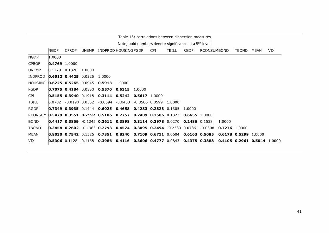
41
Table 13; correlations between dispersion measures
Note; bold numbers denote significance at a 5% level.
NGDP CPROF UNEMP INDPROD HOUSING PGDP CPI TBILL RGDP RCONSUM BOND TBOND MEAN VIX
NGDP 1.0000
CPROF 0.4769 1.0000
UNEMP 0.1279 0.1320 1.0000
INDPROD 0.6512 0.4425 0.0525 1.0000
HOUSING 0.6225 0.5265 0.0945 0.5913 1.0000
PGDP 0.7075 0.4184 0.0550 0.5570 0.6315 1.0000
CPI 0.5155 0.3940 0.1918 0.3114 0.5242 0.5617 1.0000
TBILL 0.0782 -0.0190 0.0352 -0.0594 -0.0433 -0.0506 0.0599 1.0000
RGDP 0.7349 0.3935 0.1444 0.6025 0.4658 0.4283 0.2823 0.1305 1.0000
RCONSUM 0.5479 0.3551 0.2197 0.5106 0.2757 0.2409 0.2506 0.1323 0.6655 1.0000
BOND 0.4417 0.3869 -0.1245 0.2612 0.3898 0.3114 0.3978 0.0270 0.2486 0.1538 1.0000
TBOND 0.3458 0.2602 -0.1983 0.2793 0.4574 0.3095 0.2494 -0.2339 0.0786 -0.0308 0.7276 1.0000
MEAN 0.8030 0.7542 0.1526 0.7351 0.8240 0.7109 0.6711 0.0604 0.6163 0.5085 0.6178 0.5299 1.0000
VIX 0.5306 0.1128 0.1168 0.3986 0.4116 0.3606 0.4777 0.0843 0.4375 0.3888 0.4105 0.2961 0.5044 1.0000

42
Data for excess stock returns, default premia and the VIX index are extracted from Bloomberg and
Datastream. The correlation between macro dispersion measures and the VIX can be found in table
13. Excess stock returns are measured as the quarterly S&P500 return (in %) minus the three-month
Treasury bill rate. The default premium is measured as the difference between corporate bond rates
with a Moody’s rating Baa and Aaa. This premium is measured at the end of the middle month of
each quarter. Thus, the default premium is determined about a week after the SPD deadline. Data
ranges from 1968Q4 to 2012Q4.
III.3. Method and results
III.3.1. Stock returns and macro dispersion
III.3.1.1. Is macro uncertainty remunerated in stock markets?
As mentioned under III.1.4.1, it could be interesting to check whether uncertainty (measured by
macro dispersion) is linked to higher stock market returns. At the same time, theoretical models of
Varian (1985) and Soderlind (2006) could be empirically validated. To this end, the following
equations are regressed;
𝑟(𝑡) = 𝛼 + 𝛽 ∗ 𝜎𝑥(𝑡) + 𝜀(𝑡) (1)
𝑟(𝑡) = 𝛼 + 𝛽 ∗ ∆𝜎𝑥(𝑡) + 𝜀(𝑡) (2)
Where r(t) is the excess S&P500 return over the calendar quarter t, σx is the cross-sectional
dispersion in point forecasts of variable x released in the middle of quarter t. σx is either measured
as the quasi-standard deviation or the difference in natural logs of the 16th and 84th percentile of
point forecasts. Unit root tests of these variables are presented in appendix 3. Substituting
disagreement about GDP in equation 1 is more in line with Soderlind (2006), while equation 2 is
more in line with the framework of Varian (1985). We use these specifications with a limited number
of explanatory variables to avoid multicollinearity problems, as the previously reported descriptive
statistics have shown large correlations among disagreement measures. The coefficients are
estimated with least squares, and we subsequently check for heteroscedasticity and autocorrelation.
When necessary, White heteroscedastic robust errors or Newey-West HAC errors are used. Quite
often, the hypothesis of normality is rejected for residuals. However, this doesn’t seem to be a big
problem, as the regressions generally have a quite large sample size (>100 observations). The
results of these regressions are presented in table 14.
Table 14; regressions of excess stock returns on macro disagreement
Note; *, ** and *** denote significance at a 10%, 5% or 1%, respectively.
Level of disagreement First difference of disagreement
t-stat R² t-stat R²
MEAN -0.010932 -0.202890 0.000235 -0.183650* -1.919217 0.020730
NGDP -5.363190 -0.411673 0.001674 -15.50301 -1.286658 0.009425
CPROF 0.406174 0.485592 0.002061 -0.597783 -0.897071 0.004604
UNEMP -1.225042 -0.490474 0.003576 0.627839 0.334691 0.001293

43
INDPROD 2.802401 0.698890 0.002783 -0.984196 -0.208155 0.000249
HOUSING -0.613666 -0.586915 0.003632 -1.771704* -1.96532* 0.021716
PGDP -26.95365* -1.75733* 0.018156 -35.09823** -2.0107** 0.025210
CPI -0.147099** -2.1244** 0.035119 -0.020389 -0.267420 0.000581
TBILL -0.086696 -0.470233 0.001780 0.033085 0.177233 0.000255
RGDP -7.415244 -0.891822 0.004524 -17.67908 -1.362543 0.010557
RCONSUM 0.047216 0.003638 0.000000 -18.08633 -1.317280 0.013911
BOND 0.799069 0.553533 0.003921 -0.586937 -0.438396 0.002597
TBOND 1.455678 0.989583 0.022572 -0.845234 -0.808583 0.008007
The results show only very few significant coefficients and R² statistics which are generally very low.
The MEAN index of disagreement series is significant in equation 2, but the level of significance and
R² is definitely not convincing enough to provide any generalization of this finding. The statement
therefore cannot be validated that disagreement on macro fundamentals is a form of non-diversifiable
risk. The theory of Soderlind (2006), which stated that disagreement on output should be positively
related to the equity premium, is not in line with the discussed data. Neither can the framework of
Varian (1985) be empirically validated, which stated that asset prices should decrease when
dispersion of opinion increases. Whereas micro dispersion has a clear link with stock returns, this is
far from the case for dispersion of macro estimates. The finding that dispersion in macro estimates
and stock returns are essentially unrelated, remains when controlling for different definitions of
returns (calculating returns over longer horizons, using other stock market indices), other definitions
of dispersion (standard deviation, quasi-standard deviation, inter quartile range, difference of natural
logs between the 16th and 84th percentile, using macro estimates for future quarters instead of the
current quarter, using dispersion of monthly Bloomberg macro estimates instead of SPF data) or only
taking into account quarters with extremely high disagreement levels.
Besides MEAN, two other variables in table 14 revealed significant coefficients; CPI and first
differences of PGDP. The stability of these results should be verified. After all, inflation rate has
declined significantly over time, with an average inflation of about 6% in 1981-1992 compared to
3% during the period 1992-2012. Therefore, a Chow breakpoint test is conducted (see appendix 5).
The null hypothesis of no structural break is not rejected for any of these two variables. However, it
is clear that the significance of CPI and PGDP in table 14 is not convincing enough to providing any
generalization of these findings.
III.3.1.2. Market timing strategies
Although the previous section was not able to show a link between macro dispersion and equity
returns (measured as the return over the calendar quarter in which the SPF was released), it is not
impossible that a profitable market timing strategy could be deduced from dispersion in macro
consensus data. It could still be that an investor who buys or sells equity based on macro
disagreement signals obtains positive excess returns. To this end, the following equation is
regressed;
𝑟𝑛(𝑡) = 𝛼 + 𝛽 ∗ 𝜎𝑥(𝑡) + 𝜀(𝑡) (3)
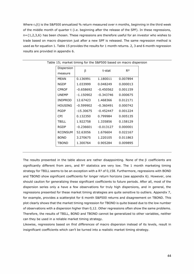
44
Where rn(t) is the S&P500 annualized % return measured over n months, beginning in the third week
of the middle month of quarter t (i.e. beginning after the release of the SPF). In these regressions,
n={1,2,3,6} has been chosen. These regressions are therefore useful for an investor who wishes to
trade based on macro dispersion just after a new SPF is released. The same regression method is
used as for equation 1. Table 15 provides the results for 1 month returns. 2, 3 and 6 month regression
results are provided in appendix 6.
Table 15; market timing for the S&P500 based on macro dispersion
Dispersion
measure t-stat R²
MEAN 0.136991 1.180011 0.007894
NGDP 1.033999 0.048249 0.000013
CPROF -0.658692 -0.450562 0.001159
UNEMP -1.150902 -0.343746 0.000675
INDPROD 12.67423 1.468366 0.012171
HOUSING -0.599902 -0.360491 0.000742
PGDP -15.30675 -0.452447 0.001224
CPI 0.132350 0.799984 0.005135
TBILL 1.922758 1.335856 0.158129
RGDP -0.236601 -0.013127 0.000001
RCONSUM 52.63056 1.676604 0.022167
BOND 3.270675 1.220105 0.011863
TBOND 1.300764 0.905284 0.009895
The results presented in the table above are rather disappointing. None of the coefficients are
significantly different from zero, and R² statistics are very low. The 1 month marketing timing
strategy for TBILL seems to be an exception with a R² of 0,158. Furthermore, regressions with BOND
and TBOND show significant coefficients for longer return horizons (see appendix 6). However, one
should caution for generalizing these significant coefficients to future periods. After all, most of the
dispersion series only a have a few observations for truly high dispersions, and in general, the
regressions presented for these market timing strategies are quite sensitive to outliers. Appendix 7,
for example, provides a scatterplot for 6 month S&P500 returns and disagreement on TBOND. This
plot clearly shows that the market timing regression for TBOND is quite biased due to the low number
of observations with a dispersion higher than 0,12. Other regressions often show the same problems.
Therefore, the results of TBILL, BOND and TBOND cannot be generalized to other variables, neither
can they be used in a reliable market timing strategy.
Likewise, regressions based on first differences of macro dispersion instead of its levels, result in
insignificant coefficients which can’t be turned into a realistic market timing strategy.

45
III.3.2. Forecast errors and macro dispersion
As stated under III.1.4.2, it has not been discussed yet in empirical literature under which conditions
macro consensus forecasts deviate from actual releases. From this perspective, it might be
interesting to check whether disagreement on macro forecasts (as a proxy for uncertainty) is
positively related to forecast error. Therefore the following regression is conducted;
|𝑒𝑟𝑟𝑜𝑟𝑥(𝑡)| = 𝛼 + 𝛽 ∗ 𝜎𝑥(𝑡) + 𝜀(𝑡) (4)
Where errorx(t), the forecast error of variable x in quarter t, is calculated by the Philadelphia SPF as
the median growth rate forecast minus the revised release. σx is the cross-sectional dispersion in
point forecasts of variable x in quarter t. Unit root tests of these variables are presented in appendix
3. The specification of equation 4, with a limited number of explanatory variables, is chosen to avoid
multicollinearity problems. White heteroscedastic robust errors or Newey-West HAC errors are used
to account for autocorrelation and/or heteroscedasticity. The results of these regressions are
presented in table 16.
Table 16; regressions of absolute forecast errors on macro disagreement
Note; *, ** and *** denote significance at a 10%, 5% or 1%, respectively.
t-stat R²
NGDP*** 253.4185 3.283708 0.139795
UNEMP 0.636403 1.632342 0.013757
INDPROD*** 112.3494 3.439826 0.091246
HOUSING 0.120485 0.898124 0.005520
PGDP*** 110.7668 3.020518 0.079860
CPI*** 1.102448 3.467397 0.301343
TBILL** 0.331731 2.289321 0.188317
RGDP*** 147.5136 3.182939 0.092194
RCONSUM* 91.75796 1.881438 0.028197
BOND*** 4.067703 3.264261 0.254957
TBOND 0.536527 1.175615 0.026864
As can be seen from the table above, all of the -coefficients have positive values and the majority
of them is significant at the 1% level. R² statistics range from 0,005 to 0,301. Thus, in general, the
hypothesis can be confirmed that larger macro uncertainty (proxied by disagreement) results in
larger forecast errors. The results remain essentially unchanged when forecast error is measured as
the difference between the median forecast and initial instead of revised release.
Besides an ordinary regression of forecast errors on macro disagreement, it was also chosen to model
a vector autoregression for each pair of error and dispersion series. The big advantage of a VAR is
that it treats the dispersion measures as being endogenous. The appropriate amount of lags were
chosen with the likelihood ratio test, Akaike information criterion, and Schwarz information criterion,
among others. In general, the models, reported in appendix 8, contain between 1 and 6 lags.
Subsequently checks for autocorrelation were undertaken using the Box-Pierce Q-statistic and the
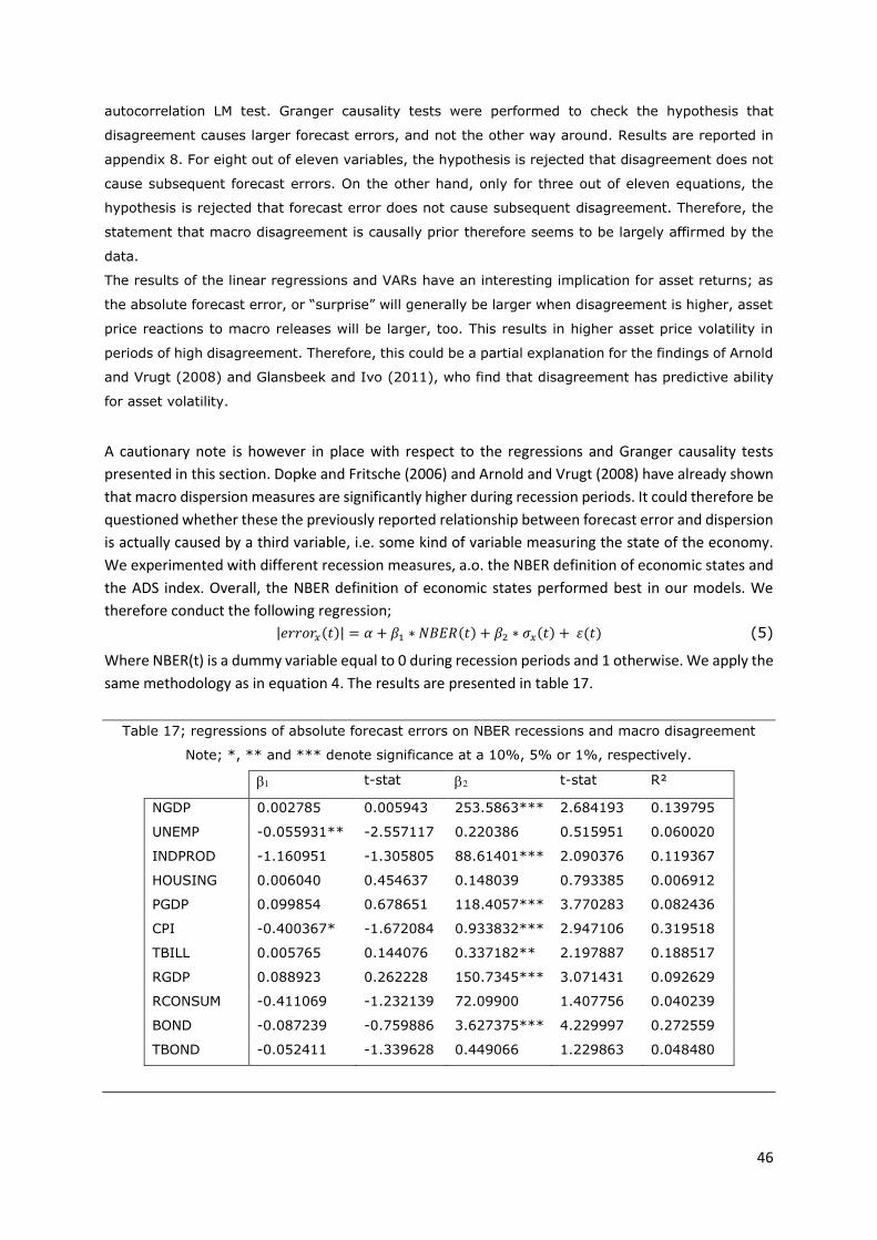
46
autocorrelation LM test. Granger causality tests were performed to check the hypothesis that
disagreement causes larger forecast errors, and not the other way around. Results are reported in
appendix 8. For eight out of eleven variables, the hypothesis is rejected that disagreement does not
cause subsequent forecast errors. On the other hand, only for three out of eleven equations, the
hypothesis is rejected that forecast error does not cause subsequent disagreement. Therefore, the
statement that macro disagreement is causally prior therefore seems to be largely affirmed by the
data.
The results of the linear regressions and VARs have an interesting implication for asset returns; as
the absolute forecast error, or “surprise” will generally be larger when disagreement is higher, asset
price reactions to macro releases will be larger, too. This results in higher asset price volatility in
periods of high disagreement. Therefore, this could be a partial explanation for the findings of Arnold
and Vrugt (2008) and Glansbeek and Ivo (2011), who find that disagreement has predictive ability
for asset volatility.
A cautionary note is however in place with respect to the regressions and Granger causality tests
presented in this section. Dopke and Fritsche (2006) and Arnold and Vrugt (2008) have already shown
that macro dispersion measures are significantly higher during recession periods. It could therefore be
questioned whether these the previously reported relationship between forecast error and dispersion
is actually caused by a third variable, i.e. some kind of variable measuring the state of the economy.
We experimented with different recession measures, a.o. the NBER definition of economic states and
the ADS index. Overall, the NBER definition of economic states performed best in our models. We
therefore conduct the following regression;
|𝑒𝑟𝑟𝑜𝑟𝑥(𝑡)| = 𝛼 + 𝛽1 ∗ 𝑁𝐵𝐸𝑅(𝑡) + 𝛽2 ∗ 𝜎𝑥(𝑡) + 𝜀(𝑡) (5)
Where NBER(t) is a dummy variable equal to 0 during recession periods and 1 otherwise. We apply the
same methodology as in equation 4. The results are presented in table 17.
Table 17; regressions of absolute forecast errors on NBER recessions and macro disagreement
Note; *, ** and *** denote significance at a 10%, 5% or 1%, respectively.
t-stat t-stat R²
NGDP 0.002785 0.005943 253.5863*** 2.684193 0.139795
UNEMP -0.055931** -2.557117 0.220386 0.515951 0.060020
INDPROD -1.160951 -1.305805 88.61401*** 2.090376 0.119367
HOUSING 0.006040 0.454637 0.148039 0.793385 0.006912
PGDP 0.099854 0.678651 118.4057*** 3.770283 0.082436
CPI -0.400367* -1.672084 0.933832*** 2.947106 0.319518
TBILL 0.005765 0.144076 0.337182** 2.197887 0.188517
RGDP 0.088923 0.262228 150.7345*** 3.071431 0.092629
RCONSUM -0.411069 -1.232139 72.09900 1.407756 0.040239
BOND -0.087239 -0.759886 3.627375*** 4.229997 0.272559
TBOND -0.052411 -1.339628 0.449066 1.229863 0.048480

47
The NBER recession measure does generally not subsume the explanatory power of dispersion
measures. Quite on the contrary, the recession measures are often insignificant, while dispersion
measures have overall highly significant t-statistics. It can therefore be stated that the previous
specification of equation 4, not including a recession measure, was correct.
III.3.3. Default premia and macro dispersion
III.3.3.1. Is the default premium linked to macro uncertainty?
As described under III.1.4.3, the fundamental models of Merton (1974) state that default premia are
positively related to volatility in a company’s value. To the extent that volatility in a firm’s value is a
proxy for uncertainty, it can be questioned whether, at a macro level, the default premium is
positively related to dispersion in macroeconomic consensus data. Previous literature on default
premia has already used the VIX as a measure of volatility or uncertainty in firm values. It might
therefore be interesting to check how well the VIX performs in comparison to disagreement as a
measure for macro uncertainty. In addition, GDP growth is introduced into the equation for the
default premium. GDP growth is expected to be significantly related to the default premium because
it proxies for the state of the economy, and therefore conveys information on the aggregate company
value in the structural model of Merton. Altogether, we regress the following equation;
𝑑𝑒𝑓𝑎𝑢𝑙𝑡(𝑡) = 𝛼 + 𝛽1 ∗ 𝑅𝑔𝑑𝑝𝑦𝑜𝑦(𝑡) + 𝛽2 ∗ 𝑉𝐼𝑋(𝑡) + 𝛽3 ∗ 𝜎𝑥(𝑡) + 𝜀(𝑡) (6)
Where the default premium, default(t), is measured as the difference between corporate bond rates
with a Moody’s rating Baa and Aaa. Rgdpyoy(t) is the year on year growth rate of Real GDP in quarter
t. σx(t) is the cross-sectional dispersion in point forecasts of variable x in quarter t. Unit root tests
for these variables are presented in appendix 3. The specification of equation 6, which only takes
into account one macro dispersion measure in every regression, is chosen to avoid multicollinearity
problems. White heteroscedastic robust errors or Newey-West HAC errors are used to account for
autocorrelation and/or heteroscedasticity.
The results of these regressions will be compared with a baseline models using RGDP growth and the
VIX;
𝑑𝑒𝑓𝑎𝑢𝑙𝑡(𝑡) = 𝛼 + 𝛽1 ∗ 𝑅𝑔𝑑𝑝𝑦𝑜𝑦(𝑡) + 𝛽2 ∗ 𝑉𝐼𝑋(𝑡) + 𝜀(𝑡) (7)
This model will be estimated using the same method as for equation 5. The results of these
regressions are presented in table 18.
Table 18; regressions of default premia on GDP growth, VIX and macro disagreement
Note; *, ** and *** denote significance at a 10%, 5% or 1%, respectively. Values in parentheses
are HAC corrected t statistics.
Dispersion
measure 1 t-stat 2 t-stat 3 t-stat R² Adj. R²
Eq. (5) -14.306*** -6.0562 0.0208*** 4.2845 0.7229 0.7166
MEAN -6.9857*** -3.1921 0.0162*** 3.9236 0.6447*** 4.0080 0.7748 0.7671
NGDP -12.429*** -5.0546 0.0192*** 3.6472 37.895 1.3084 0.7315 0.7223
CPROF -11.630*** -4.8486 0.0222*** 4.8485 2.1254*** 2.7880 0.7459 0.7373
UNEMP -14.438*** -6.1128 0.0212*** 4.5692 -3.2804* -1.9474 0.7299 0.7207
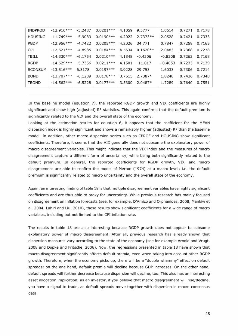
48
INDPROD -12.916*** -5.2487 0.0201*** 4.1059 9.3777 1.0614 0.7271 0.7178
HOUSING -11.749*** -5.9089 0.0190*** 4.2022 2.7373** 2.0528 0.7421 0.7333
PGDP -12.956*** -4.7422 0.0205*** 4.2026 34.771 0.7847 0.7259 0.7165
CPI -12.621*** -4.8985 0.0184*** 4.5534 0.1620** 2.0483 0.7368 0.7278
TBILL -14.330*** -6.1754 0.0210*** 4.1848 -0.4306 -0.8308 0.7262 0.7168
RGDP -14.629*** -5.7356 0.0211*** 4.1501 -11.017 -0.4053 0.7233 0.7139
RCONSUM -13.516*** 6.3178 0.0197*** 3.9228 29.753 1.6033 0.7306 0.7214
BOND -13.707*** -6.1289 0.0178*** 3.7615 2.7387* 1.8248 0.7436 0.7348
TBOND -14.562*** -6.5228 0.0177*** 3.5300 2.0487* 1.7289 0.7640 0.7551
In the baseline model (equation 7), the reported RGDP growth and VIX coefficients are highly
significant and show high (adjusted) R² statistics. This again confirms that the default premium is
significantly related to the VIX and the overall state of the economy.
Looking at the estimation results for equation 6, it appears that the coefficient for the MEAN
dispersion index is highly significant and shows a remarkably higher (adjusted) R² than the baseline
model. In addition, other macro dispersion series such as CPROF and HOUSING show significant
coefficients. Therefore, it seems that the VIX generally does not subsume the explanatory power of
macro disagreement variables. This might indicate that the VIX index and the measures of macro
disagreement capture a different form of uncertainty, while being both significantly related to the
default premium. In general, the reported coefficients for RGDP growth, VIX, and macro
disagreement are able to confirm the model of Merton (1974) at a macro level; i.e. the default
premium is significantly related to macro uncertainty and the overall state of the economy.
Again, an interesting finding of table 18 is that multiple disagreement variables have highly significant
coefficients and are thus able to proxy for uncertainty. While previous research has mainly focused
on disagreement on inflation forecasts (see, for example, D’Amico and Orphanides, 2008, Mankiw et
al. 2004, Lahiri and Liu, 2010), these results show significant coefficients for a wide range of macro
variables, including but not limited to the CPI inflation rate.
The results in table 18 are also interesting because RGDP growth does not appear to subsume
explanatory power of macro disagreement. After all, previous research has already shown that
dispersion measures vary according to the state of the economy (see for example Arnold and Vrugt,
2008 and Dopke and Fritsche, 2006). Now, the regressions presented in table 18 have shown that
macro disagreement significantly affects default premia, even when taking into account other RGDP
growth. Therefore, when the economy picks up, there will be a “double whammy” effect on default
spreads; on the one hand, default premia will decline because GDP increases. On the other hand,
default spreads will further decrease because dispersion will decline, too. This also has an interesting
asset allocation implication; as an investor, if you believe that macro disagreement will rise/decline,
you have a signal to trade, as default spreads move together with dispersion in macro consensus
data.

49
Following the extant literature, more macro variables could be included into a specification for the
default premium. For example, S&P500 returns could be included as a measure for the business
climate (see e.g. Bhar et al., 2011). The rate on 10 year Treasury bond returns is also often used to
explain default premia (see e.g. Longstaff and Schwartz, 1995 and Collin-Dufresne et al. 2001).
Lastly, as the term premium is associated to economic activity (i.e. a lower term premium indicates
a higher probability of a recession), it can also be related to default premia (see e.g., Duffee, 1998
and Papageorgiou and Skinner (2006). Therefore, the following specification is regressed;
𝑑𝑒𝑓𝑎𝑢𝑙𝑡(𝑡) = 𝛼 + 𝛽1 ∗ 𝑟𝑔𝑑𝑝𝑦𝑜𝑦(𝑡) + 𝛽2 ∗ 𝑆𝑃𝑋(𝑡) + 𝛽3 ∗ ∆𝑇𝑏𝑜𝑛𝑑(𝑡)+
𝛽4 ∗ 𝑇𝑒𝑟𝑚(𝑡) + 𝛽5 ∗ 𝑉𝐼𝑋(𝑡) + 𝛽6 ∗ 𝜎𝑀𝐸𝐴𝑁(𝑡) + 𝜀(𝑡) (8)
Where SPX(t) is the quarterly S&P500 return; Tbond(t) is the yield on a 10 year Treasury bond;
Term(t) is the difference between the rate of a 10 year Treasury bond and a 3 month T Bill. All of
these variables are measured at the end of the second month of quarter t. In this extended
specification, it is chosen to only model the MEAN disagreement index, without any other dispersion
measures. Newey-West HAC errors are used to account for heteroscedasticity and autocorrelation.
Table 19 presents the results.
Table 19; default premium regressed on its macro determinants
Note; *** denotes significance at 1% level. HAC corrected t-statistics are given in parentheses.
1 2 3 4 5 6 0.1431 -6.8684*** -0.2845 0.0544 0.0153 0.0159*** 0.6279***
(0.6199) (-3.2804) (-0.7191) (1.4330) (0.7922) (4.1945) (3.6732)
R²= 0.781981 ; Adj. R² = 0.766592
As it appears from the table above, the three additional macro variables don’t add explanatory power
to our initial specification presented in equation 6. Their t-statistics are insignificant, and the
(adjusted) R² remains essentially unchanged compared to the results of table 18. Therefore, we
reject this specification and keep our original regression of equation 6.
III.3.3.2. Market timing strategies
As the previous section has shown a significant relationship between default premia and macro
uncertainty, it can be questioned whether disagreement in macro estimates can also be used for a
market timing strategy. Similar to III.3.1.2, we model the following regression;
∆𝑛𝑠𝑝𝑟𝑒𝑎𝑑(𝑡) = 𝛼 + 𝛽 ∗ 𝜎𝑥(𝑡) + 𝜀(𝑡) (9)
Where nspread(t) is the difference in the default spread (in percentage point) measured over n
months, beginning in the third week of the middle month of quarter t (i.e. beginning after the release
of the SPF). In these regressions, n={1,2,3,6} has been chosen. These regressions are therefore
useful for an investor who wishes to trade based on macro dispersion just after a new SPF is released.
The same regression method is used as for equation 6. Table 20 provides the results for 1 month
default spread changes. 2, 3 and 6 month regression results are provided in appendix 9.
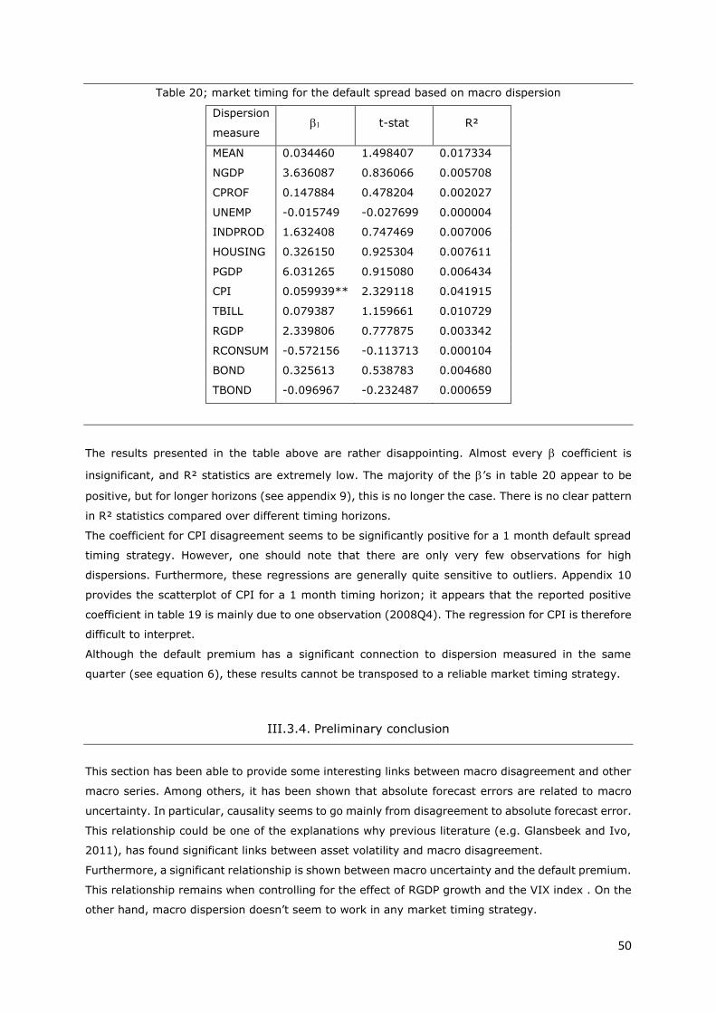
50
Table 20; market timing for the default spread based on macro dispersion
Dispersion
measure t-stat R²
MEAN 0.034460 1.498407 0.017334
NGDP 3.636087 0.836066 0.005708
CPROF 0.147884 0.478204 0.002027
UNEMP -0.015749 -0.027699 0.000004
INDPROD 1.632408 0.747469 0.007006
HOUSING 0.326150 0.925304 0.007611
PGDP 6.031265 0.915080 0.006434
CPI 0.059939** 2.329118 0.041915
TBILL 0.079387 1.159661 0.010729
RGDP 2.339806 0.777875 0.003342
RCONSUM -0.572156 -0.113713 0.000104
BOND 0.325613 0.538783 0.004680
TBOND -0.096967 -0.232487 0.000659
The results presented in the table above are rather disappointing. Almost every coefficient is
insignificant, and R² statistics are extremely low. The majority of the ’s in table 20 appear to be
positive, but for longer horizons (see appendix 9), this is no longer the case. There is no clear pattern
in R² statistics compared over different timing horizons.
The coefficient for CPI disagreement seems to be significantly positive for a 1 month default spread
timing strategy. However, one should note that there are only very few observations for high
dispersions. Furthermore, these regressions are generally quite sensitive to outliers. Appendix 10
provides the scatterplot of CPI for a 1 month timing horizon; it appears that the reported positive
coefficient in table 19 is mainly due to one observation (2008Q4). The regression for CPI is therefore
difficult to interpret.
Although the default premium has a significant connection to dispersion measured in the same
quarter (see equation 6), these results cannot be transposed to a reliable market timing strategy.
III.3.4. Preliminary conclusion
This section has been able to provide some interesting links between macro disagreement and other
macro series. Among others, it has been shown that absolute forecast errors are related to macro
uncertainty. In particular, causality seems to go mainly from disagreement to absolute forecast error.
This relationship could be one of the explanations why previous literature (e.g. Glansbeek and Ivo,
2011), has found significant links between asset volatility and macro disagreement.
Furthermore, a significant relationship is shown between macro uncertainty and the default premium.
This relationship remains when controlling for the effect of RGDP growth and the VIX index . On the
other hand, macro dispersion doesn’t seem to work in any market timing strategy.
51
It is somewhat surprising that we found a significant relationship between macro uncertainty and
default spreads, while such a significant relationship has not been found for stock returns. From a
theoretical perspective, however, the risk priced in stock markets should be fundamentally connected
to default premia. This goes back to Merton (1974), who relates the default premium to the volatility
in firm value. Jarrow and Turnbull (2000, p. 272) also state that “If the market value of the firm’s
assets unexpectedly changes – generating market risk – this affects the probability of default –
generating credit risk. Conversely, if the probability of default unexpectedly changes – generating
credit risk – this affects the market value of the firm – generating market risk.” In empirical research,
a significant link between aggregate stock returns and the default premium has already been found
by Shane (1994), Huang and Kong (2003), Collin-Dufresne et al. (2001) and Bhar and Handzic
(2011). From this perspective, it remains puzzling that it was not possible to relate macro uncertainty
to stock returns.
III.4. Conclusion
This chapter started with an overview of a wide range in literature showing a clear link between stock
returns and dispersion in micro consensus data. Several authors such as Ackert and Athanassakos
(1997), Diether et al. (2002) and Hintikka (2008) have shown that shares with a lower disagreement
about earnings forecasts will outperform the stock market. This finding is backed by several
independent theoretical models on micro dispersion, such as the frameworks of Miller (1997) and
Johnson (2004).
Where previous research came up with clear asset allocation strategies for micro dispersion, this is
far from the case for macro dispersion. There are some theoretical models on the link between macro
dispersion and stock returns (see e.g. Varian, 1985 and Soderlind, 2006), but these models have
generally remained without empirical validation. The extant empirical literature has previously
performed research on the link between dispersion and recession periods (e.g. Dopke and Fritsche,
2006), dispersion and asset volatility (e.g. Glansbeek and Ivo, 2011), dispersion and term premia
(D’Amico and Orphanides, 2008) and dispersion and levels of inflation (e.g. Mankiw et al. 2004).
In this thesis, literature on macro dispersion is augmented by showing that disagreement has a clear
link with future macro surprises and default spreads. Previous empirical literature (e.g. D’Amico and
Orphanides, 2008, Mankiw et al. 2004, Lahiri and Liu, 2010) has mainly focused on disagreement on
inflation forecasts. An interesting finding of this thesis is that disagreement in other macro variables
is equally useful in empirical research. Also, an index of macro dispersion, as suggested by Bowles
et al. (2007) provides significant coefficients in most of the models tested in this chapter.
Altogether, in line with papers by Zarnowitz and Lambros (1987), Giordani and Soderlind (2003),
Arnold and Vrugt (2008), Glansbeek and Ivo (2011), and Dopke and Fritsche (2006), the results
presented in this thesis can be seen as additional evidence that disagreement on macro estimates is
a good proxy for uncertainty.

52
Another part of this chapter focused on the link between excess stock returns and dispersion in macro
consensus data. These regressions, however, were not able to provide significant results. Therefore
it was not possible to empirically validate research by Varian (1985) or Soderlind (2006). Hence,
macro uncertainty (proxied by disagreement) does not appear to be a source of non-diversifiable
risk. Furthermore, dispersion in macro estimates does not appear to be useful for stock market
timing, nor default spread timing.
Any further research that could explain why the tests for excess stock market returns were not able
to provide significant coefficients, or any research that could nevertheless empirically demonstrate a
link between macro uncertainty and equity returns, would be very helpful.
VII
REFERENCES
Ackert L. and Athanassakos G., 1997, Prior Uncertainty, Analyst Bias, and Subsequent Abnormal
Returns, The Journal of Financial Research 20(2), pp. 263-273.
Adams G., McQueen G. and Wood R.,2004, The Effects of Inflation News on High Frequency Stock
Returns, Journal of Business 77(3), pp. 547-574.
Andersen T., Bollerslev T., Diebold F., Vega C., 2003, Micro effects of macro announcements: real-
time price discovery in foreign exchange, American Economic Review 93(1), pp. 38-62.
Andersen T., Bollerslev T., Diebold F., Vega C., 2007, Real-time price discovery in global stock, bond
and foreign exchange markets, Journal of International Economics 73(2), pp. 251-277.
Anderson E., Ghysels E. and Juergens J., 2005, Do Heterogeneous Beliefs Matter for Asset Pricing?,
Review of Financial Studies 18(3), pp. 875-924.
Anderson E., Ghysels E. and Juergens J., 2009, The impact of risk and uncertainty on expected
returns, Journal of Financial Economics 94(2), pp. 233-263.
Andersson M., Overby L., Sebestyen S., 2009, Which news moves the Euro area bond market?,
German Economic Review 10, pp. 1-31.
Ang A. and Bekaert G., 2007, Stock Return Predictability: Is it There?, Review of Financial Studies
20(3), pp. 651-707.
Ang J. and Ciccone S., 2001, Analyst Forecasts and Stock Returns, working paper.
Arnold I. and Vrugt E., 2008, Fundamental uncertainty and stock market volatility, Applied Financial
Economics 18(17), pp. 1425-1440.
Asprem M. ,1989, Stock prices, asset portfolios and macroeconomic variables in ten European
countries, Journal of Banking and Finance 13(4), pp. 589-612.
Baker S., Bloom N. and Davis S., 2012, Measuring Economic Policy Uncertainty, working paper.
Balduzzi P., Elton E., and Green C., 2001, Economic News and Bond Prices: Evidence from the U.S.
Treasury Market, Journal of Financial and Quantitative Analysis 36(4), pp. 523-543.
Balvers R., Cosimano T., McDonald B.,1990, Predicting Stock Returns in an Efficient Market, Journal
of Finance 45(4), pp. 1109-1128.
Berben, R., van Dijk, D., 1998. Does the absence of cointegration explain the typical findings in long
horizon regressions? Erasmus University Rotterdam report 9814.
Berkman H., Dimitrov V., Jain P., Koch P., Tice S., 2009, Sell on the news: Differences of opinion,
short-sales constraints, and returns around earnings announcements, Journal of Financial Economics
92(3), pp. 376-399.
Berkowitz J., and Giorgianni L., 2001, Long-Horizon Exchange Rate Predictability?, Review of
Economics and Statistics 83(1), pp. 81-91.
Bhar, R. and Handzic, N., 2011, A multifactor model of credit spreads, Asia-Pacific Financial Markets
18(2), pp. 105-127.
Binswanger M., 2004, Stock returns and real activity in the G-7 countries: did the relationship change
during the 1980s?, The Quarterly Review of Economics and Finance 44(2), pp. 237-252.
Black F. and Cox J., 1976, Valuing Corporate Securities: Some Effects of Bond Indenture Provisions,
Journal of Finance 31(2), pp. 351-367.
VIII
Bowles C., Friz R., Genre V., Kenny G., Meyler A. and Rautanen T., 2007, The ECB survey of
professional forecasters (SPF) a review after eight years’ experience, ECB Occasional Paper Series
59.
Boyd J., Hu J., Jagannathan R., 2005, The Stock Market’s Reaction to Unemployment News: Why
Bad News Is Usually Good for Stocks, Journal of Finance 60(2), pp. 649-672.
C. Nelson, 1976, Inflation and the rates of return on common stock, The Journal of Finance 31(2),
pp. 471-483.
Capistran C. and Timmermann A., 2009, Disagreement and Biases in Inflation Expectations, Journal
of Money, Credit and Banking 41(2), pp. 365-396.
Cathcart L. and El-Jahel L., 1998, Valuation of defaultable bonds, Journal of Fixed Income 8(1), pp.
65-78.
Cenesizoglu T., 2011, Size, book-to-market ratio and macroeconomic news, Journal of Empirical
Finance 18(2), pp. 248-270.
Chahine S., 2004, Dispersion of analysts’ forecasts and the profitability of trading strategies around
the preannouncement, Journal of Multinational Financial Management, pp. 67-79.
Chang K.L., 2009, Do macroeconomic variables have regime-dependent effects on stock return
dynamics? Evidence from the Markov regime switching model, Economic Modeling 26(6), pp. 1283-
1299.
Chen N.,1991, Financial Investment Opportunities and the Macroeconomy, Journal of Finance 46(2),
pp. 529-554.
Chen S.S., 2007, Does Monetary Policy Have Asymmetric Effects on Stock Returns?, Journal of
Money, Credit and Banking 39(2), pp. 667-688.
Chen S.S., 2009, Predicting the bear stock market: Macroeconomic variables as leading indicators,
Journal of Banking and Finance 33(2), pp. 211-223.
Cheung Y., Chinn M., and Pascual A., 2005, Empirical exchange rate models of the nineties: Are any
fit to survive?, Journal of International Money and Finance 24(7), pp. 1150-1175.
Chinn M. and Meese R., 1995, Banking on currency forecasts: How predictable is change in money?,
Journal of International Economics 38(1), pp. 161-178.
Chong Y., Jorda O. and Taylor A., 2012, The Harrod–Balassa–Samuelson hypothesis: real exchange
rates and their long-run equilibrium, International Economic Review 55(2), pp. 609-634.
Collin-Dufresne P., Goldstein R. and Marin S., 2001, The Determinants of Credit Spread Changes,
Journal of Finance 56(6), pp. 2177-2207.
Conover C., Jensen G., Johnson R., 1999, Monetary environments and international stock returns,
Journal of Banking and Finance 23(9), pp. 1357-1381.
Croushore, D., 1993, Introducing: the survey of professional forecasters, Federal Reserve Bank of
Philadelphia Business Review 1993(6), pp. 3–15.
Cutler D., Poterba J. and Summers L., 1989, What moves stock prices?, The Journal of Portfolio
Management 15(3), pp. 4-12.
D’Amico S. and Orphanides A., 2008, Uncertainty and Disagreement in Economic Forecasting,
working paper.
Das S. and Tufano P., 1996, Pricing credit sensitive debt when interest rates, credit ratings and credit
spreads are stochastic, Journal of Financial Engineering 5(2), pp. 161–198

IX
David A., 2008, Heterogeneous beliefs, speculation, and the equity premium, The Journal of Finance
63(1), pp. 41-83.
Detemple J. and Murthy S., 1994, Intertemporal Asset Pricing with Heterogeneous Beliefs, Journal
of Economic Theory 62(2), pp. 294-320.
Diether K., Malloy C. and Scherbina A., 2002, Differences of Opinion and the Cross Section of Stock
Returns, Journal of Finance 57(5), pp. 2113-2141.
Dische A., 2002, Dispersion in analyst forecasts and the profitability of earnings momentum
strategies, European Financial Management 8(2), pp. 211-228.
Dopke I. and Fritsche U., 2006, When do forecasters disagree? An assessment of German growth
and inflation forecast dispersion, International Journal of Forecasting, 22(1), pp. 125-135.
Dopke, J. and Fritsche, U., 2006, When do forecasters disagree? An assessment of German growth
and inflation forecast dispersion, International Journal of Forecasting 22(1), pp. 125-135.
Doukas J., Kim C. and Pantzalis C., 2004, Divergent opinions and the performance of value stocks,
Financial Analysts Journal 60(6), pp. 55-64.
Drine I. and Rault C., 2005, Can the Balassa-Samuelson theory explain long-run real exchange rate
movements in OECD countries?, Applied Financial Economics 15(8), pp. 519-530.
Duffee G., 1998, The relationship between treasury yields and corporate bond yield spreads, Journal
of Finance 53(6), pp. 2225-2241.
Dumrongrittikul T., 2012, Real Exchange Rate Movements in Developed and Developing Economies:
A Reinterpretation of the Balassa-Samuelson Hypothesis, Economic Record 88, pp. 537-553.
Durham, 2001, The Effect of Monetary Policy on Monthly and Quarterly Stock Market Returns: Cross-
Country Evidence and Sensitivity Analyses, Federal Reserve Discussion Paper.
Ehrmann M. and Fratzscher M. ,2005, Equal Size, Equal Role? Interest Rate Interdependence
Between the Euro Area and the United States, Economic Journal 115(506), pp. 928-948.
Ewing B., 2003, The response of the default risk premium to macroeconomic shocks, The Quarterly
Review of Economics and Finance 43(2), pp. 261-272.
Fama E. and French K., 1989, Business conditions and expected returns on stocks and bonds, Journal
of Financial Economics 25(1), pp. 23-49.
Fama E. and MacBeth J., 1973, Risk, Return, and Equilibrium: Empirical Tests, The Journal of Political
Economy 81(3), pp. 607-636.
Fama E., 1981, Stock Returns, Real Activity, Inflation, and Money, The American Economic Review
71(4), pp. 545-565.
Fama E., 1990, Stock Returns, Expected Returns, and Real Activity, Journal of Finance 45(4), pp.
189-1108.
Fama E., Schwert G., 1977, Asset returns and inflation, Journal of Financial Economics 5(2), pp. 115-
146.
Faust J., Rogers J., Wang S., and Wright J., 2007, The high-frequency response of exchange rates
and interest rates to macroeconomic announcements, Journal of Monetary Economics 54(4), pp.
1051-1068.
Fifield, S., Power D., Sinclair C., 2000, A study of whether macroeconomic factors influence emerging
market share returns, Global Economy Quarterly 1(1): 315-335.
Flannery M. and Protopapadakis A., 2002, Macroeconomic Factors Do Influence Aggregate Stock
Returns, Review of Financial Studies 15(3), pp. 751-782.

X
Gharghori P., See Q. and Veeraraghavan M., 2011, Difference of opinion and the cross-section of
equity returns: Australian evidence, Pacific-Basin Finance Journal 19(4), pp. 435-446.
Giordani P. and Soderlind P., 2003, Inflation forecast uncertainty, European Economic Review 47(6),
pp. 1037-1059.
Giordani P. and Soderlind P., 2006, Is there evidence of pessimism and doubt in subjective
distributions? Implications for the equity premium puzzle, Journal of Economic Dynamics and Control
30(6), pp. 1027-1043.
Glansbeek M. and Ivo A., 2011, The ECB’s survey of professional forecasters and financial market
volatility in the euro area, Applied Economic Letters 18(1), pp. 11-15.
Güntay L. and Hackbarth D., 2010, Corporate bond credit spreads and forecast dispersion, Journal
of Banking and Finance 34(10), pp. 2328-2345.
Hautsch, N., and Hess D. (2002), The processing of non-anticipated information in financial markets:
Analyzing the impact of surprises in the employment report, European Finance Review 6(2), pp. 133-
161.
Hintikka M., 2008, Market reactions to differences of opinion, working paper.
Humpe A. and Macmillan P.,2009, Can macroeconomic variables explain long-term stock market
movements? A comparison of the US and Japan, Applied Financial Economics 19(2), pp. 111-119.
Jarrow R. and Turnbull, S., 2000, The intersection of market and credit risk, Journal of Banking and
Finance 24(1), pp. 271-299.
Johnson T., 2004, Forecast Dispersion and the Cross Section of Expected Returns, Journal of Finance
59(5), pp. 1957-1978.
Kaneko T. and Lee B. S., 1995, Relative importance of economic-factors in the U.S. and Japanese
stock markets, Journal of the Japanese and International Economies 9(3), pp. 290-307.
Kaul G., 1987, Stock returns and inflation - The role of the monetary sector, Journal of Financial
Economics, 18(2), pp. 253-276.
Kilian L., 1999, Exchange rates and monetary fundamentals: what do we learn from long-horizon
regressions?, Journal of Applied Econometrics 14(5), pp. 491-510.
Kim B. and Mo S., 1995, Cointegration and the long-run forecast of exchange rates, Economics
Letters 48(3), pp. 353-359.
Kim S., McKenzie M. and Faff R., 2004, Macroeconomic news announcements and the role of
expectations: evidence for US bond, stock and foreign exchange markets, Journal of Multinational
Financial Management 14(3), pp. 217-232.
Lahiri K. and Liu F., 2010, ARCH Models for Multi-period Forecast Uncertainty -- A Reality Check
Using a Panel of Density Forecasts, in Terrell D. and Fomby B., Econometric Analysis of Financial and
Economic Time Series, Emerald Group Publishing, pp. 321-363.
Lahiri K. and Sheng X., 2010, Measuring Forecast Uncertainty By Disagreement: The Missing Link,
Journal of Applied Econometrics 25(4), pp. 514-538.
Laster, D., Bennett, P. and Geoum, I. (1999) Rational bias in macroeconomic forecasts, Quarterly
Journal of Economics, 114, 293–318.
Lee B. S., 1992, Causal relations among stock returns, interest-rates, real activity, and inflation,
Journal of Finance 47(4), pp. 1591-1603.
Leippold M. and Lohre H., 2012, The Dispersion Effect in International Stock Returns, working paper.
XI
Longstaff F. and Schwartz E., 1995, A simple approach to valuing risky fixed and floating rate debt,
Journal of Finance 50(3), pp. 789-819.
MacDonald R. and Taylor M., 1994, The monetary model of the exchange rate: long-run relationships,
short-run dynamics and how to beat a random walk, Journal of International Money and Finance
13(6), pp. 276-290.
Mankiw G., Reis R., Wolfers J., 2004, Disagreement on inflation expectations, NBER Macroeconomics
Annual 2003 (18), pp. 209-270.
Marathe and Shawky ,1994, Predictability of stock returns and real output, The Quarterly Review of
Economics and Finance 34(4), pp. 317-331.
Mark N. and Sul D., 2001, Nominal exchange rates and monetary fundamentals - Evidence from a
small post-Bretton woods panel, Journal of International Economics 53(1), pp. 29-52.
Mark N., 1995, Exchange rates and fundamentals: Evidence on long-horizon predictability, The
American Economic Review 85(1), pp. 201-218.
McQueen G., and Roley V., 1993, Stock Prices, News, and Business Conditions, Review of Financial
Studies 6(3), pp. 683-707.
Meese R. and Rogoff K.,1983, Empirical exchange rate models of the seventies - Do they fit out of
sample?, Journal of International Economics 14(1), pp. 3-24.
Merton R., 1974, On the pricing of corporate debt: The risk structure of interest rates, Journal of
Finance 29(2), pp.449-470.
Merton R., 1977, On the pricing of contingent claims and the Modigliani-Miller theorem, Journal of
Financial Economics 5(2), pp. 241-249.
Miller E., 1977, Risk, Uncertainty, and Divergence of Opinion, Journal of Finance 32(4), pp. 1151-
1168.
Molodtsova T. and Papell D., 2009, Out-of-sample exchange rate predictability with Taylor rule
fundamentals, Journal of International Economics 77(2), pp. 167-180.
Molodtsova T., Nikolsko A. and Papell D., 2008, Taylor rules with real-time data: A tale of two
countries and one exchange rate, Journal of Monetary Economics 55, pp. S63-S79.
Nasseh A. and Strauss J., 2000, Stock prices and domestic and international macroeconomic activity:
a cointegration approach, the Quarterly Review of Economics and Finance 40(2), pp. 229-245.
Nikolsko-Rzhevskyy A., Prodan R., 2012, Markov switching and exchange rate predictability,
International Journal of Forecasting 28(2), pp. 353-365.
Papageorgiou N. and Skinner F., 2006, Credit spreads and the zero-coupon treasury spot curve,
Journal of Financial Research 29(3), pp. 421-439.
Pearce D. and Roley V., 1983, The Reaction of Stock Prices to Unanticipated Changes in Money: A
Note, Journal of Finance 38(4), pp. 1323-1333.
Pearce D. and Roley V., 1985, Stock Prices and Economic News, Journal of Business 58(1), pp. 49-
67.
Pedrosa M. and Roll R., 1998, Systematic Risk in Corporate Bond Credit Spreads, Journal of Fixed
Income 8(3), pp. 7-26.
Perez-Quiros G. and Timmermann A., 2000, Firm Size and Cyclical Variations in Stock Returns,
Journal of Finance 55(3), pp. 1229-1262.
Pesaran H. and Timmermann A., 1992, A Simple Nonparametric Test of Predictive Performance,
Journal of Business and Economic Statistics 10(4), pp. 461-465.

XII
Poitras M., 2004, The Impact of Macroeconomic Announcements on Stock Prices: In Search of State
Dependence, Southern Economic Journal 70(3), pp. 549-565.
Rapach, Wohar, Rangvid ,2005, Macro variables and international stock return predictability,
International Journal of Forecasting 21(1), pp. 137-166.
Resnick B. and Shoesmith G., 2002, Using the Yield Curve to Time the Stock Market, Financial
Analysts Journal 58(3), pp. 82-90.
Schwert W.,1990, Stock Returns and Real Activity: A Century of Evidence, Journal of Finance 45(4),
pp. 1237-1257.
Scotti C., 2012, Surprise and Uncertainty Indexes: Real-time Aggregation of Real-Activity Macro
Surprises, working paper.
Siklos P. and Kwok B., 1999, Stock returns and inflation: a new test of competing hypotheses, Applied
Financial Economics 9(6), pp. 567-581.
Soderlind P., 2009, Why disagreement may not matter (much) for asset prices, Finance Research
Letters 6(2), pp. 73-82.
Solanes J., Portero F. and Flores F., 2008, Beyond the Balassa-Samuelson effect in some new
member states of the European Union 32(1), pp. 17-32.
Solnick B., 1984, The relationship between stock prices and inflationary expectations: The
international evidence, the Journal of Finance 38(1), pp. 35-38.
Varian H., 1985, Divergence of Opinion in Complete Markets: A Note, Journal of Finance 40(1), pp.
309-317.
Wasserfallen W.,1989, Macroeconomic news and the stock market: Evidence for Europe, Journal of
Banking and Finance 13(4), pp. 613-626.
Zarnowitz V. and Lambros L., 1987, Consensus and Uncertainty in Economic Prediction, The Journal
of Political Economy 95(3), pp. 591-621.
Zhang F., 2006, Information Uncertainty and Stock Returns, Journal of Finance 61(1), pp. 105-137.
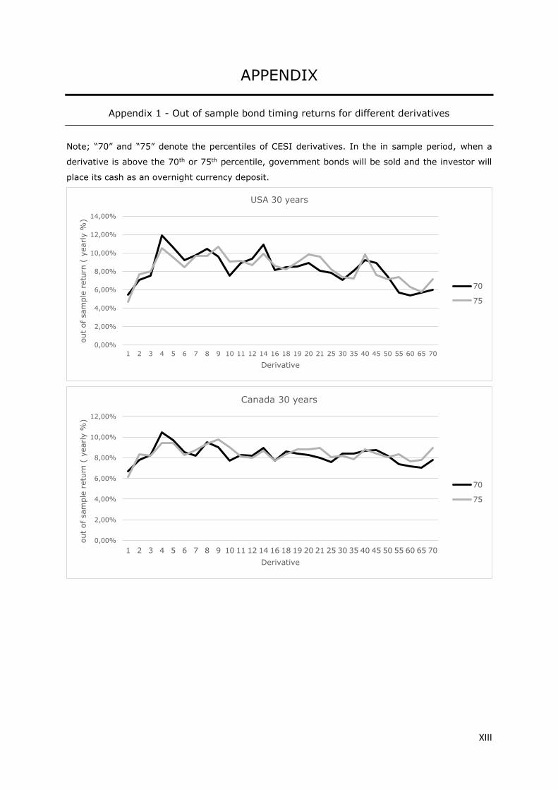
XIII
APPENDIX
Appendix 1 - Out of sample bond timing returns for different derivatives
Note; “70” and “75” denote the percentiles of CESI derivatives. In the in sample period, when a
derivative is above the 70th or 75th percentile, government bonds will be sold and the investor will
place its cash as an overnight currency deposit.
0,00%
2,00%
4,00%
6,00%
8,00%
10,00%
12,00%
14,00%
1 2 3 4 5 6 7 8 9 10 11 12 14 16 18 19 20 21 25 30 35 40 45 50 55 60 65 70
out
of sam
ple
retu
rn (
yearly %
)
Derivative
USA 30 years
70
75
0,00%
2,00%
4,00%
6,00%
8,00%
10,00%
12,00%
1 2 3 4 5 6 7 8 9 10 11 12 14 16 18 19 20 21 25 30 35 40 45 50 55 60 65 70
out
of sam
ple
retu
rn (
yearly %
)
Derivative
Canada 30 years
70
75
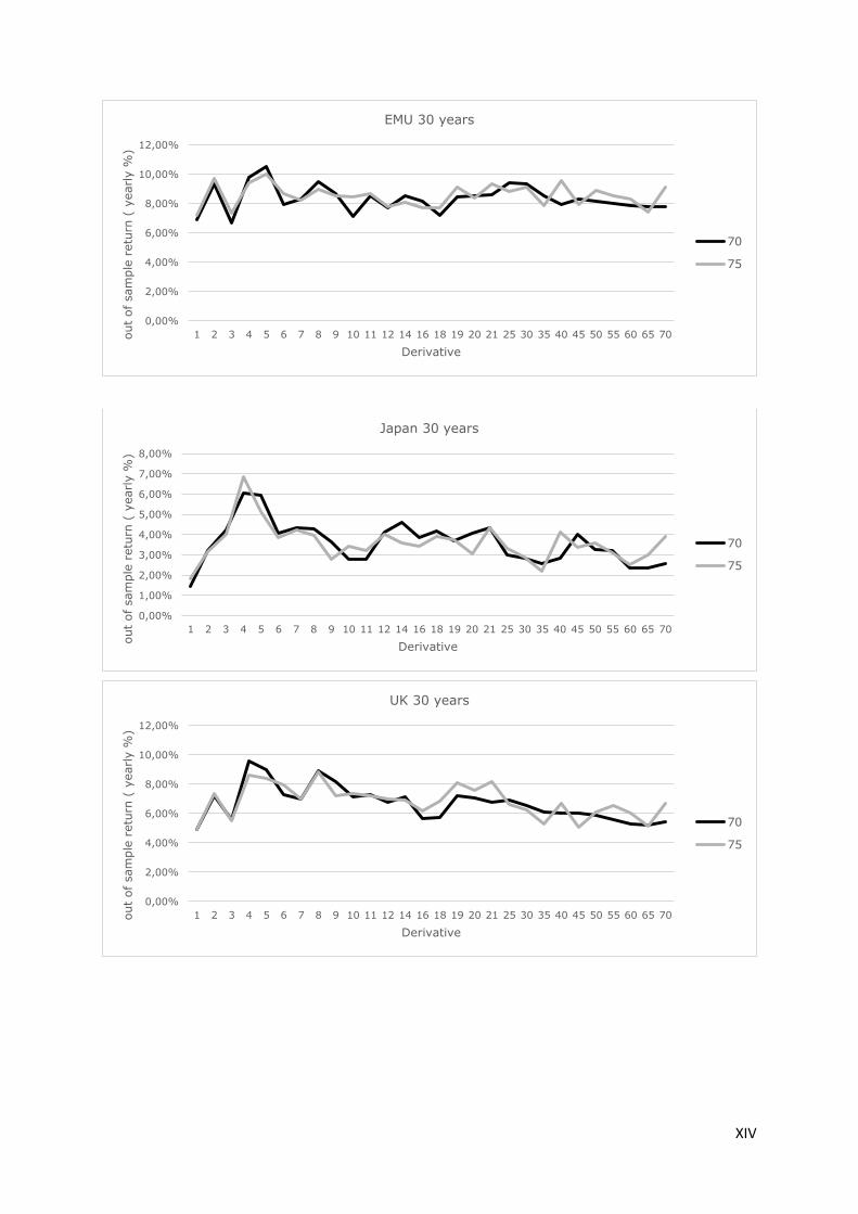
XIV
0,00%
2,00%
4,00%
6,00%
8,00%
10,00%
12,00%
1 2 3 4 5 6 7 8 9 10 11 12 14 16 18 19 20 21 25 30 35 40 45 50 55 60 65 70out
of sam
ple
retu
rn (
yearly %
)
Derivative
EMU 30 years
70
75
0,00%
1,00%
2,00%
3,00%
4,00%
5,00%
6,00%
7,00%
8,00%
1 2 3 4 5 6 7 8 9 10 11 12 14 16 18 19 20 21 25 30 35 40 45 50 55 60 65 70
out
of sam
ple
retu
rn (
yearly %
)
Derivative
Japan 30 years
70
75
0,00%
2,00%
4,00%
6,00%
8,00%
10,00%
12,00%
1 2 3 4 5 6 7 8 9 10 11 12 14 16 18 19 20 21 25 30 35 40 45 50 55 60 65 70out
of sam
ple
retu
rn (
yearly %
)
Derivative
UK 30 years
70
75
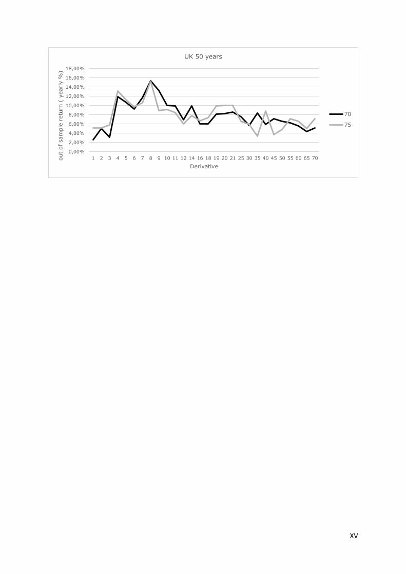
XV
0,00%
2,00%
4,00%
6,00%
8,00%
10,00%
12,00%
14,00%
16,00%
18,00%
1 2 3 4 5 6 7 8 9 10 11 12 14 16 18 19 20 21 25 30 35 40 45 50 55 60 65 70out
of sam
ple
retu
rn (
yearly %
)
Derivative
UK 50 years
70
75
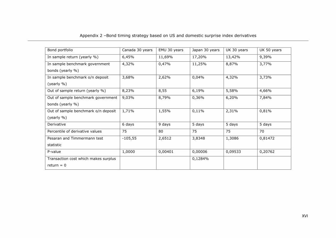
XVI
Appendix 2 –Bond timing strategy based on US and domestic surprise index derivatives
Bond portfolio Canada 30 years EMU 30 years Japan 30 years UK 30 years UK 50 years
In sample return (yearly %) 6,45% 11,69% 17,20% 13,42% 9,39%
In sample benchmark government
bonds (yearly %)
4,32% 0,47% 11,25% 8,87% 3,77%
In sample benchmark o/n deposit
(yearly %)
3,68% 2,62% 0,04% 4,32% 3,73%
Out of sample return (yearly %) 8,23% 8,55 6,19% 5,58% 4,66%
Out of sample benchmark government
bonds (yearly %)
9,03% 8,79% 0,36% 6,20% 7,84%
Out of sample benchmark o/n deposit
(yearly %)
1,71% 1,55% 0,11% 2,31% 0,81%
Derivative 6 days 9 days 5 days 5 days 5 days
Percentile of derivative values 75 80 75 75 70
Pesaran and Timmermann test
statistic
-105,55 2,6512 3,8348 1,3086 0,81472
P-value 1,0000 0,00401 0,00006 0,09533 0,20762
Transaction cost which makes surplus
return = 0
0,1284%
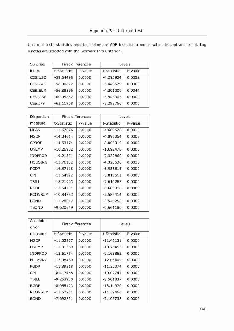
XVII
Appendix 3 - Unit root tests
Unit root tests statistics reported below are ADF tests for a model with intercept and trend. Lag
lengths are selected with the Schwarz Info Criterion.
Surprise
index
First differences Levels
t-Statistic P-value t-Statistic P-value
CESIUSD -59.64498 0.0000 -4.295934 0.0032
CESICAD -58.90872 0.0000 -5.440529 0.0000
CESIEUR -56.88596 0.0000 -4.201009 0.0044
CESIGBP -60.05852 0.0000 -5.943305 0.0000
CESIJPY -62.11908 0.0000 -5.298766 0.0000
Dispersion
measure
First differences Levels
t-Statistic P-value t-Statistic P-value
MEAN -11.67676 0.0000 -4.689528 0.0010
NGDP -14.04614 0.0000 -4.896064 0.0005
CPROF -14.53474 0.0000 -8.005310 0.0000
UNEMP -10.26932 0.0000 -10.92476 0.0000
INDPROD -19.21301 0.0000 -7.332860 0.0000
HOUSING -13.76182 0.0000 -4.325636 0.0036
PGDP -16.87118 0.0000 -6.955815 0.0000
CPI -11.64922 0.0000 -5.819661 0.0000
TBILL -18.21903 0.0000 -7.610267 0.0000
RGDP -13.54701 0.0000 -6.686918 0.0000
RCONSUM -10.84753 0.0000 -7.585414 0.0000
BOND -11.78617 0.0000 -3.546256 0.0389
TBOND -9.620649 0.0000 -6.661180 0.0000
Absolute
error
measure
First differences Levels
t-Statistic P-value t-Statistic P-value
NGDP -11.02267 0.0000 -11.46131 0.0000
UNEMP -11.01369 0.0000 -10.75453 0.0000
INDPROD -12.61764 0.0000 -9.163862 0.0000
HOUSING -13.08469 0.0000 -12.06409 0.0000
PGDP -11.89318 0.0000 -11.32074 0.0000
CPI -8.417468 0.0000 -10.02741 0.0000
TBILL -9.263930 0.0000 -8.501837 0.0000
RGDP -8.055123 0.0000 -13.14970 0.0000
RCONSUM -13.67281 0.0000 -11.39460 0.0000
BOND -7.692831 0.0000 -7.105738 0.0000

XVIII
TBOND -6.546613 0.0000 -10.89335 0.0000
First differences Levels
t-Statistic P-value t-Statistic P-value
Default -14.39212 0.0000 -4.216240 0.0052
Rgdpyoy -7.140652 0.0000 -3.588521 0.0339
VIX -8.229661 0.0000 -5.147136 0.0003
Tbond -12.43731 0.0000 -12.63894 0.0000
Term -13.21141 0.0000 -3.763947 0.0208
SPX -15.39542 0.0000 -11.58876 0.0000
Appendix 4 –Bond timing strategy based on surprise index levels
In the tables below, levels of the CESIUSD are divided into different “hurdles” or percentiles. The
corresponding mean future government bond returns are calculated. These future bond returns are
defined as the percentage change over a horizon of 2 weeks and 1, 2, 3 and 6 months. Arbitrarily,
the hurdles are chosen as the 10th, 20th, 80th and 90th percentiles of CESIUSD levels. The average
government bond return is presented in the middle row of each table.
USA government bonds and CESIUSD
CESI percentile 2 weeks 1 month 2 months 3 months 6 months
0,9 0,4246% 0,6122% 0,5866% 2,2617% 6,5553%
0,8 0,4415% 0,7583% 0,9946% 2,5075% 6,3829%
average 0,3092% 0,6267% 1,2434% 1,8851% 3,7896%
0,2 0,5936% 1,0974% 1,2019% 0,9304% 1,8272%
0,1 1,3467% 2,5693% 3,1951% 2,7545% 3,3502%
Canadian government bonds and CESIUSD
CESI percentile 2 weeks 1 month 2 months 3 months 6 months
0,9 0,4490% 0,5360% 0,6355% 1,7984% 4,6134%
0,8 0,3576% 0,5060% 0,7147% 1,9243% 4,8013%
average 0,3391% 0,6794% 1,3384% 2,0367% 4,1687%
0,2 0,4945% 0,9836% 1,4594% 1,8503% 3,5063%
0,1 1,0043% 1,9154% 2,9146% 3,3355% 4,8761%
EMU government bonds and CESIUSD
CESI percentile 2 weeks 1 month 2 months 3 months 6 months
0,9 0,1135% 0,3264% 0,5564% 1,8660% 4,7383%
0,8 0,3069% 0,5809% 1,1389% 2,4517% 5,4048%
average 0,3275% 0,6452% 1,2796% 1,9911% 4,1630%
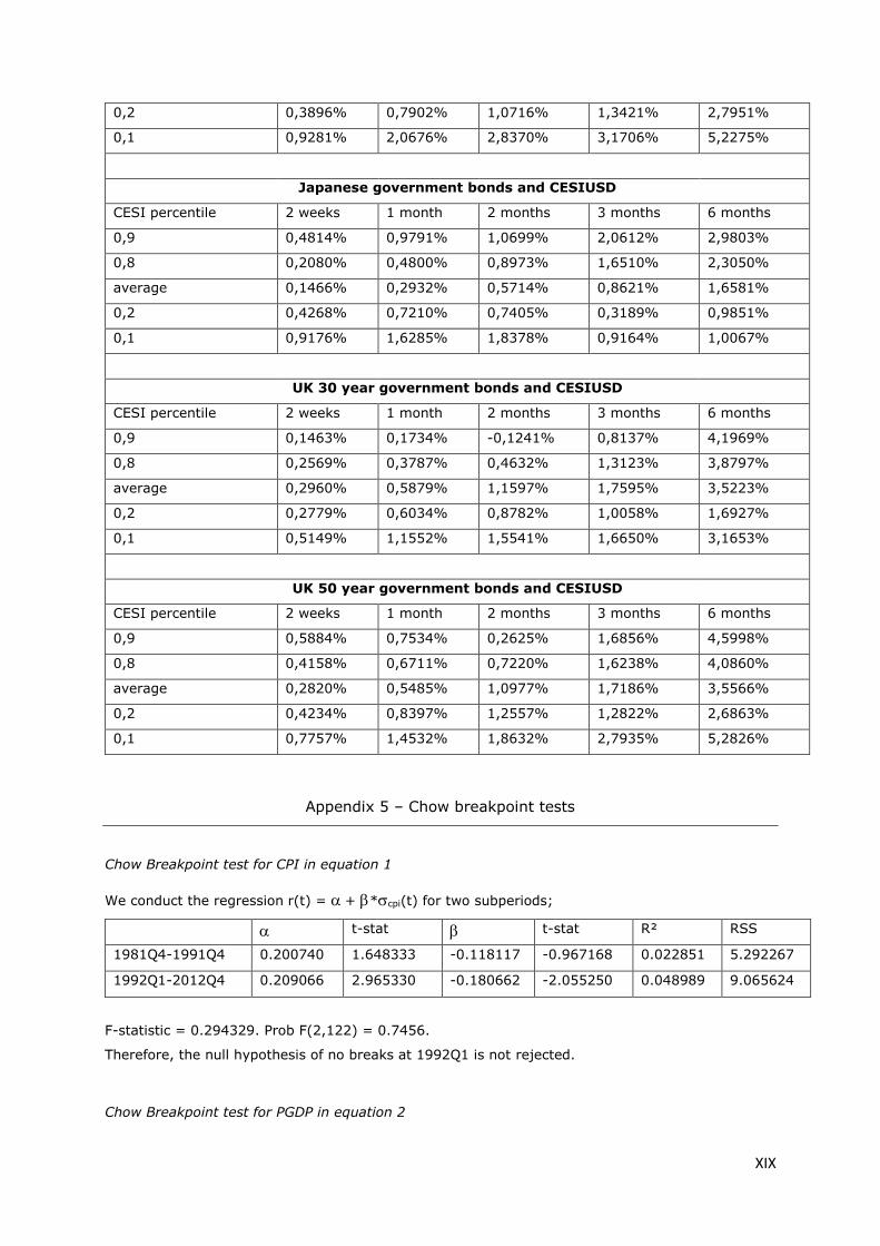
XIX
0,2 0,3896% 0,7902% 1,0716% 1,3421% 2,7951%
0,1 0,9281% 2,0676% 2,8370% 3,1706% 5,2275%
Japanese government bonds and CESIUSD
CESI percentile 2 weeks 1 month 2 months 3 months 6 months
0,9 0,4814% 0,9791% 1,0699% 2,0612% 2,9803%
0,8 0,2080% 0,4800% 0,8973% 1,6510% 2,3050%
average 0,1466% 0,2932% 0,5714% 0,8621% 1,6581%
0,2 0,4268% 0,7210% 0,7405% 0,3189% 0,9851%
0,1 0,9176% 1,6285% 1,8378% 0,9164% 1,0067%
UK 30 year government bonds and CESIUSD
CESI percentile 2 weeks 1 month 2 months 3 months 6 months
0,9 0,1463% 0,1734% -0,1241% 0,8137% 4,1969%
0,8 0,2569% 0,3787% 0,4632% 1,3123% 3,8797%
average 0,2960% 0,5879% 1,1597% 1,7595% 3,5223%
0,2 0,2779% 0,6034% 0,8782% 1,0058% 1,6927%
0,1 0,5149% 1,1552% 1,5541% 1,6650% 3,1653%
UK 50 year government bonds and CESIUSD
CESI percentile 2 weeks 1 month 2 months 3 months 6 months
0,9 0,5884% 0,7534% 0,2625% 1,6856% 4,5998%
0,8 0,4158% 0,6711% 0,7220% 1,6238% 4,0860%
average 0,2820% 0,5485% 1,0977% 1,7186% 3,5566%
0,2 0,4234% 0,8397% 1,2557% 1,2822% 2,6863%
0,1 0,7757% 1,4532% 1,8632% 2,7935% 5,2826%
Appendix 5 – Chow breakpoint tests
Chow Breakpoint test for CPI in equation 1
We conduct the regression r(t) = + *cpi(t) for two subperiods;
t-stat t-stat R² RSS
1981Q4-1991Q4 0.200740 1.648333 -0.118117 -0.967168 0.022851 5.292267
1992Q1-2012Q4 0.209066 2.965330 -0.180662 -2.055250 0.048989 9.065624
F-statistic = 0.294329. Prob F(2,122) = 0.7456.
Therefore, the null hypothesis of no breaks at 1992Q1 is not rejected.
Chow Breakpoint test for PGDP in equation 2
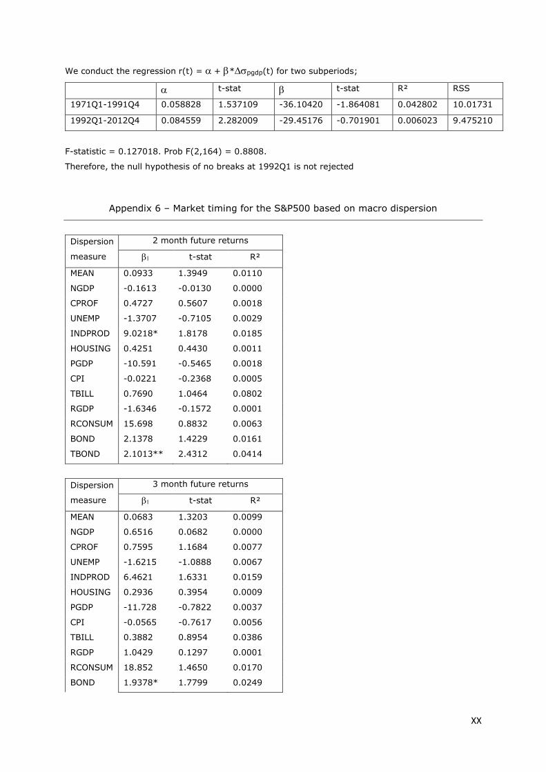
XX
We conduct the regression r(t) = + *pgdp(t) for two subperiods;
t-stat t-stat R² RSS
1971Q1-1991Q4 0.058828 1.537109 -36.10420 -1.864081 0.042802 10.01731
1992Q1-2012Q4 0.084559 2.282009 -29.45176 -0.701901 0.006023 9.475210
F-statistic = 0.127018. Prob F(2,164) = 0.8808.
Therefore, the null hypothesis of no breaks at 1992Q1 is not rejected
Appendix 6 – Market timing for the S&P500 based on macro dispersion
Dispersion
measure
2 month future returns
t-stat R²
MEAN 0.0933 1.3949 0.0110
NGDP -0.1613 -0.0130 0.0000
CPROF 0.4727 0.5607 0.0018
UNEMP -1.3707 -0.7105 0.0029
INDPROD 9.0218* 1.8178 0.0185
HOUSING 0.4251 0.4430 0.0011
PGDP -10.591 -0.5465 0.0018
CPI -0.0221 -0.2368 0.0005
TBILL 0.7690 1.0464 0.0802
RGDP -1.6346 -0.1572 0.0001
RCONSUM 15.698 0.8832 0.0063
BOND 2.1378 1.4229 0.0161
TBOND 2.1013** 2.4312 0.0414
Dispersion
measure
3 month future returns
t-stat R²
MEAN 0.0683 1.3203 0.0099
NGDP 0.6516 0.0682 0.0000
CPROF 0.7595 1.1684 0.0077
UNEMP -1.6215 -1.0888 0.0067
INDPROD 6.4621 1.6331 0.0159
HOUSING 0.2936 0.3954 0.0009
PGDP -11.728 -0.7822 0.0037
CPI -0.0565 -0.7617 0.0056
TBILL 0.3882 0.8954 0.0386
RGDP 1.0429 0.1297 0.0001
RCONSUM 18.852 1.4650 0.0170
BOND 1.9378* 1.7799 0.0249
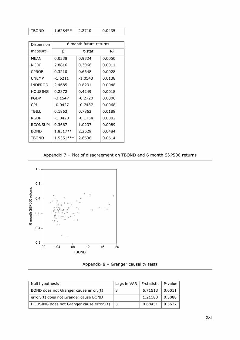
XXI
TBOND 1.6284** 2.2710 0.0435
Dispersion
measure
6 month future returns
t-stat R²
MEAN 0.0338 0.9324 0.0050
NGDP 2.8816 0.3966 0.0011
CPROF 0.3210 0.6648 0.0028
UNEMP -1.6211 -1.0543 0.0138
INDPROD 2.4685 0.8231 0.0048
HOUSING 0.2872 0.4249 0.0018
PGDP -3.1547 -0.2720 0.0006
CPI -0.0427 -0.7487 0.0068
TBILL 0.1863 0.7862 0.0188
RGDP -1.0420 -0.1754 0.0002
RCONSUM 9.3667 1.0237 0.0089
BOND 1.8517** 2.2629 0.0484
TBOND 1.5351*** 2.6638 0.0614
Appendix 7 – Plot of disagreement on TBOND and 6 month S&P500 returns
Appendix 8 – Granger causality tests
Null hypothesis Lags in VAR F-statistic P-value
BOND does not Granger cause errorx(t) 3 5.71513 0.0011
errorx(t) does not Granger cause BOND 1.21180 0.3088
HOUSING does not Granger cause errorx(t) 3 0.68451 0.5627
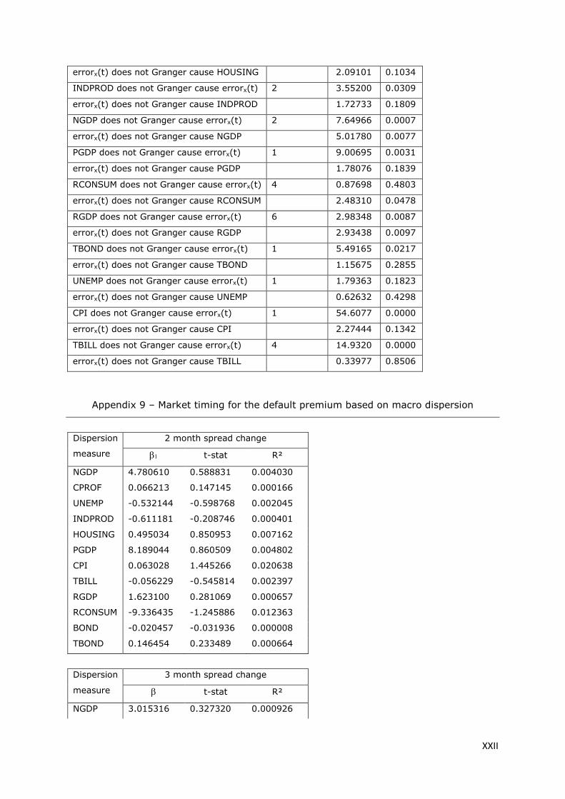
XXII
errorx(t) does not Granger cause HOUSING 2.09101 0.1034
INDPROD does not Granger cause errorx(t) 2 3.55200 0.0309
errorx(t) does not Granger cause INDPROD 1.72733 0.1809
NGDP does not Granger cause errorx(t) 2 7.64966 0.0007
errorx(t) does not Granger cause NGDP 5.01780 0.0077
PGDP does not Granger cause errorx(t) 1 9.00695 0.0031
errorx(t) does not Granger cause PGDP 1.78076 0.1839
RCONSUM does not Granger cause errorx(t) 4 0.87698 0.4803
errorx(t) does not Granger cause RCONSUM 2.48310 0.0478
RGDP does not Granger cause errorx(t) 6 2.98348 0.0087
errorx(t) does not Granger cause RGDP 2.93438 0.0097
TBOND does not Granger cause errorx(t) 1 5.49165 0.0217
errorx(t) does not Granger cause TBOND 1.15675 0.2855
UNEMP does not Granger cause errorx(t) 1 1.79363 0.1823
errorx(t) does not Granger cause UNEMP 0.62632 0.4298
CPI does not Granger cause errorx(t) 1 54.6077 0.0000
errorx(t) does not Granger cause CPI 2.27444 0.1342
TBILL does not Granger cause errorx(t) 4 14.9320 0.0000
errorx(t) does not Granger cause TBILL 0.33977 0.8506
Appendix 9 – Market timing for the default premium based on macro dispersion
Dispersion
measure
2 month spread change
t-stat R²
NGDP 4.780610 0.588831 0.004030
CPROF 0.066213 0.147145 0.000166
UNEMP -0.532144 -0.598768 0.002045
INDPROD -0.611181 -0.208746 0.000401
HOUSING 0.495034 0.850953 0.007162
PGDP 8.189044 0.860509 0.004802
CPI 0.063028 1.445266 0.020638
TBILL -0.056229 -0.545814 0.002397
RGDP 1.623100 0.281069 0.000657
RCONSUM -9.336435 -1.245886 0.012363
BOND -0.020457 -0.031936 0.000008
TBOND 0.146454 0.233489 0.000664
Dispersion
measure
3 month spread change
t-stat R²
NGDP 3.015316 0.327320 0.000926
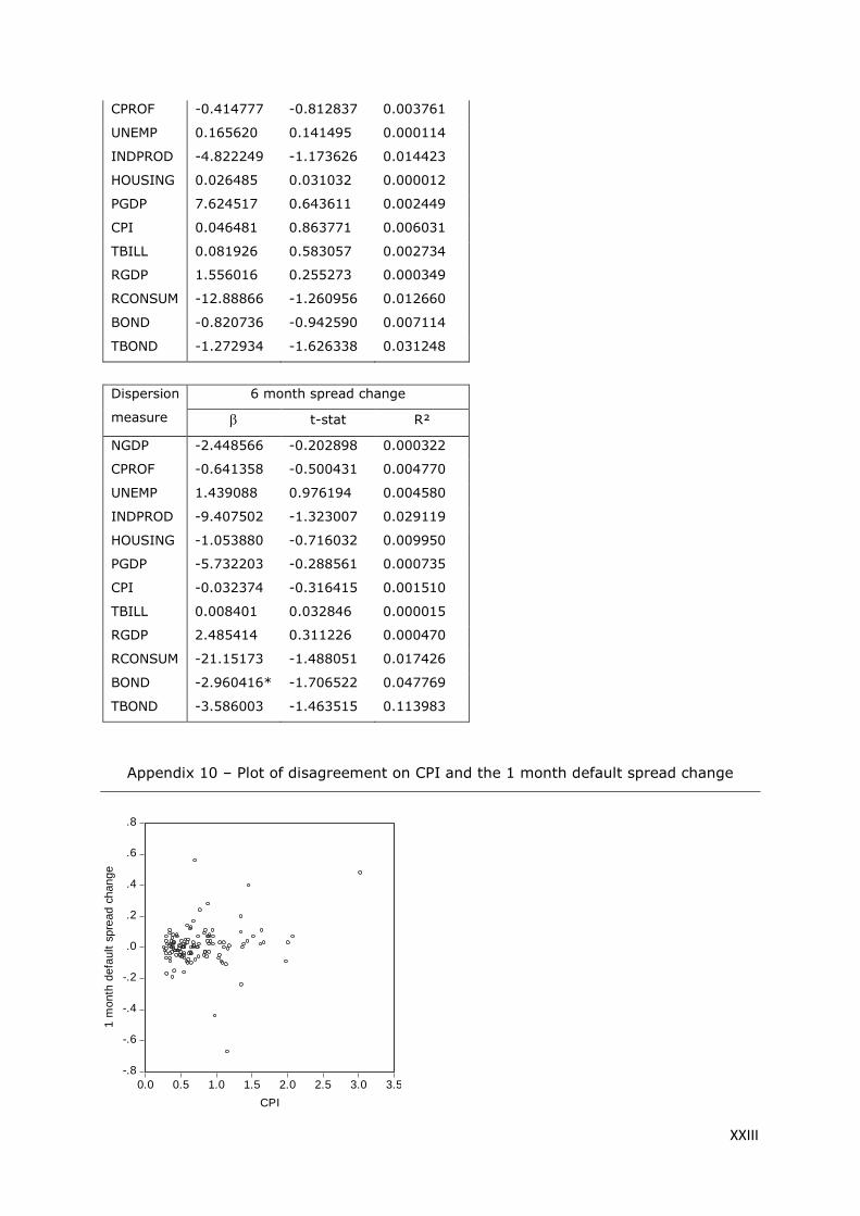
XXIII
CPROF -0.414777 -0.812837 0.003761
UNEMP 0.165620 0.141495 0.000114
INDPROD -4.822249 -1.173626 0.014423
HOUSING 0.026485 0.031032 0.000012
PGDP 7.624517 0.643611 0.002449
CPI 0.046481 0.863771 0.006031
TBILL 0.081926 0.583057 0.002734
RGDP 1.556016 0.255273 0.000349
RCONSUM -12.88866 -1.260956 0.012660
BOND -0.820736 -0.942590 0.007114
TBOND -1.272934 -1.626338 0.031248
Dispersion
measure
6 month spread change
t-stat R²
NGDP -2.448566 -0.202898 0.000322
CPROF -0.641358 -0.500431 0.004770
UNEMP 1.439088 0.976194 0.004580
INDPROD -9.407502 -1.323007 0.029119
HOUSING -1.053880 -0.716032 0.009950
PGDP -5.732203 -0.288561 0.000735
CPI -0.032374 -0.316415 0.001510
TBILL 0.008401 0.032846 0.000015
RGDP 2.485414 0.311226 0.000470
RCONSUM -21.15173 -1.488051 0.017426
BOND -2.960416* -1.706522 0.047769
TBOND -3.586003 -1.463515 0.113983
Appendix 10 – Plot of disagreement on CPI and the 1 month default spread change
-.8
-.6
-.4
-.2
.0
.2
.4
.6
.8
0.0 0.5 1.0 1.5 2.0 2.5 3.0 3.5
CPI
1 m
on
th d
efa
ult
sp
rea
d c
ha
ng
e

XXIV
Appendix 11 – Nederlandse samenvatting
Macro verrassingen
Macro-economische voorspellingen hebben aanzienlijk meer aandacht gekregen in recent empirisch
onderzoek. Dit type van data is namelijk zeer nuttig om het verband tussen macro verrassingen en
rendementen van verschillende activa klassen te onderzoeken.
Het literatuuronderzoek in deel II.1 toont dat vele academische publicaties gebruik maken van
conventionele fundamentele modellen of gewone levels in macro variabelen om een verband te
onderzoeken tussen asset returns en macro-economische variabelen. Dit type onderzoek resulteerde
echter in veel insignificante variabelen. Anderzijds, publicaties die gebruik maakten van macro
verrassingen waren wel in staat om consistente resultaten aan te tonen. Forex rendementen,
bijvoorbeeld, hebben een sterk verband met een brede waaier aan macro verrassingen.
Fundamentele modellen voor forex waren daarentegen niet in staat om systematisch goede
resultaten aan te tonen.
Literatuur over macro verrassingen heeft vaak de interactie tussen verrassingen van verschillende
variabelen genegeerd. Daarom heeft deze thesis gebruikt gemaakt van indices van macro
verrassingen om zo een nieuwe methode voor te stellen om het verband tussen activa rendementen
en macro verrassingen te onderzoeken. De descriptieve analyse van deel II.2 toont aan dat aandelen,
forex en obligaties een duidelijk verband hebben met indices van macro verrassingen.
In deel II.3 wordt een obligatie timing strategie voorgesteld, gebaseerd op de afgeleide van de
CESIUSD index. De resultaten tonen aan dat, voordat transactiekosten in rekening worden gebracht,
deze strategie hoge abnormale rendementen behaalt voor verschillende portefeuilles van lange
termijn overheidsobligaties. Deze timing strategie heeft echter ook beperkingen. De afgeleide wordt
in deze modellen gedefinieerd als het verschil in index niveau over 5 of 6 dagen. Deze korte termijn
definitie zorgt daarom bijvoorbeeld voor hoge transactiekosten.
Gerelateerde obligatie timing modellen die gebaseerd zijn op indices van macro verrassingen van
andere landen dan de USA, of modellen gebaseerd op het niveau (“hurdle”) van indices van macro
verrassingen, zijn vaak niet winstgevend.
In elk geval tonen de positieve resultaten van het obligatie timing model, gebaseerd op de eerste
afgeleide van de CESIUSD, dat macro surprise indices potentieel hebben om gebruikt te worden in
asset allocatie beslissingen.
Verder onderzoek over indices van macro verrassingen zou betrekking kunnen hebben op een meer
formele (descriptieve) analyse over het verband tussen deze indices en activa rendementen. Market
timing modellen voor andere activa klassen, zoals aandelen kunnen ook interessant zijn. Hierbij is
het vooral een uitdaging om het tijdsafhankelijk verband te modelleren dat vaak wordt gevonden in
onderzoek over macro verrassingen en aandelenreturns. Klaarblijkelijk zijn er verschillende

XXV
mogelijke invalshoeken om indices van macro verrassingen verder te bestuderen. Verder onderzoek
kan interessante applicaties hebben voor asset allocatie beslissingen.
Dispersie & consensus data
Dit deel begint met een literatuuronderzoek over de invloed van micro consensusdata op
aandelenrendementen. Verschillende auteurs zoals Ackert en Athanassakos (1997), Diether et al.
(2002) en Hintikka (2008) hebben aangetoond dat aandelen met een lage dispersie in
winstvoorspellingen gemiddeld hogere rendementen zullen genereren. Deze empirische bevinding
worden ondersteund door theoretische modellen van micro dispersie, waaronder de theorie van Miller
(1977) en Johnson (2004).
Alhoewel academisch onderzoek in staat is geweest om duidelijke asset allocatie strategieën te
formuleren voor micro dispersie, is dit lang niet het geval voor dispersie in macro voorspellingen. Er
zijn wel enkele theoretische modellen die het verband tussen macro dispersie en
aandelenrendementen behandelen (bv. Varian, 1985 en Soderlind, 2006). Echter, deze modellen
werden niet empirisch gevalideerd. De emprische literatuur over macro dispersie heeft reeds een
verbanden aangetoond tussen dispersie en economische recessies (bv. Dopke en Fritsche, 2006),
dispersie en volatiliteit in verschillende activa klassen (bv. Glansbeek en Ivo, 2011), dispersie en de
term premium (D’Amico en Orphanides, 2008) en dispersie en inflatie (bv. Mankiw et al. 2004).
Deze thesis draagt bij tot de literatuur over macro dispersie door aan te tonen dat dispersie in macro
voorspellingen een duidelijk verband heeft met macro verrassingen en default spreads. Vorig
onderzoek heeft vooral een focus op dispersie in inflatie voorspellingen (bv. D’Amico en Orphanides,
2008, Mankiw et al. 2004, Lahiri en Liu, 2010). Een interessante bevinding van deze thesis is dat
dispersie in andere macro variabelen even nuttig kan zijn voor academisch onderzoek. Verder wordt
er ook aangetoond dat een index van gemiddelde macro dispersie eveneens significante resultaten
toont in de meeste modellen van dit hoofdstuk.
In overeenstemming met ander onderzoek door Zarnowitz en Lambros (1987), Giordani en Soderlind
(2003), Arnold en Vrugt (2008), Glansbeek en Ivo (2011), en Dopke en Fritsche (2006), tonen de
resultaten van deze masterproef aan dat dispersie in macro consensus data een goede proxy is voor
onzekerheid.
Een volgend deel van deze thesis behandelde het verband tussen aandelenrendementen en dispersie
in macro consensus data. Deze regressies toonden echter geen significant resultaat. Het was dus
niet mogelijk om de publicaties van Varian (1985) of Soderlind (2009) empirisch te valideren. Macro
onzekerheid blijkt met andere woorden geen vorm van niet-diversifieerbaar risico te zijn.
Daarenboven kan dispersie in macro voorspellingen niet gebruikt worden voor een stock market
timing of default spread timing strategie.
Verder onderzoek dat zou kunnen uitleggen waarom aandelenrendementen geen significant verband
hebben met macro dispersie, of elk onderzoek dat toch een link tussen macro onzekerheid en
aandelenrendementen zou kunnen aantonen, zou in dit opzicht zeer nuttig zijn.

XXV
Top Related