


Languages
Pages
Legal


HERO
Fighting Transient Epidemics Optimal Vaccination Schedules Before and After an Outbreak Eric Nævdal Department of Economics, University of Oslo UNIVERSITY OF OSLO HEALTH ECONOMICS RESEARCH PROGRAMME Working paper 2006: 6

Fighting Transient Epidemics
Optimal Vaccination Schedules Before and After an Outbreak
Eric Nævdal
Health Economics Research Programme at the University of Oslo HERO 2006
Author`s address: Department of Economics and HERO, University of Oslo P.O. Box 1095 Blindern, N-0317 Oslo, Norway E-mail: [email protected]
Acknowledgment: The author gratefully acknowledges financial support from the Research Council of Norway through HERO – Health Economic Research
Programme at the University of Oslo.
© 2006 HERO and the authors – Reproduction is permitted when the source is referred to. Health Economics Research Programme at the University of Oslo
Financial support from The Research Council of Norway is acknowledged. ISSN 1501-9071, ISBN 82-7756-167-9
Introduction Throughout history, epidemics have been a recurring terror to humanity. In
vulnerable societies prior to the development of modern medicine an epidemic could
wipe out 50-60% of a population. With the possible exception of AIDS, modern
epidemics are less devastating to affected communities, but still impose large costs on
society. Even more mundane diseases such as influenza impose large costs. A bad
outbreak of the flu that causes, say, 10% of the population to loose on average 5
working days, represents a severe economic cost to society no matter how trivial the
disease is. On the other hand, viruses such as the Ebola virus with a fatality rate
close to 90% cause considerable harm to small contained areas even if the extreme
mortality in itself prevents the disease from spreading to affect large populations.
Recent diseases such as SARS and the possibility of a bird flu epidemic have
underscored the importance of transient epidemics to human welfare.
One common feature of many epidemics is that they tend to move through a
population and then disappear. The epidemic may reappear later, possibly in a
mutated form, but still represents disjoint events. To my knowledge this class of
epidemic has not yet been analysed in the economic literature. Often outbreaks these
epidemics are predicted, leading to the additional question of how to implement
preparatory health policies anticipating the outbreak. The present paper thus fills
two important gaps in the literature. First we analyse optimal vaccination policy for
an epidemic that eradicates itself. Second, we analyse optimal preparatory
vaccination schedules. Optimal preventive policies are likely to depend on parameters
that are intrinsically uncertain. Here we first analyse the deterministic case and use
this analysis as a stepping stone for the case where there is uncertainty about if and
when the epidemic starts as well as about the parameters in the model.
The economic literature on the subject is concerned with two issues.1 What is the
optimal health policy from society’s perspective and what private incentives exist for
individuals to take preventive measures such as vaccinating themselves? Brito et al
(1991), and Geoffard and Philipson (1996) examine vaccination policies. Gerzowitz
1 There is a huge mathematical and biological literature on the control of epidemics. Unfortunately
this literature often applies objectives and methods that most economists would not recognize as
appropriate for economic analysis.
2

and Hammer (2004) examine the case of several instruments. Here it is focused on
optimal public health policies. That is, what is the optimal vaccination program a
society should undertake before and after the outbreak of an epidemic? An
underlying assumption is that vaccination programs can be enforced by fiat. The
analysis that comes closest is the class of epidemics that are eradicable, but remain
endemic in the absence of policy intervention. Goldman and Lightwood (2002),
Barrett and Hoel (2006).
There are three standard approaches to analysing optimal control problems in
economic theory:
1) Using analytical methods to find a closed form solution
2) Drawing a phase diagram
3) Steady state analysis.
Unfortunately none of these methods work with the problem at hand. No analytical
solutions can be found that solve the problem. A phase diagram only works with
problems where there is only one state-variable and the current problem has two.
Steady state analysis does not work either, since we then analyse a system where
there are no infections either because the epidemic has not started or the epidemic is
over and these are not the most interesting cases.2
The Kermac-McKendrick model of epidemic diseases. A classical models of epidemics is named after the authors of Kermac and
McKendrick (1927). Several variations of the model exist to describe epidemics with
different properties with respect to mortality, immunity and time horizon. In the
present paper only one of these variations are examined. Consider an epidemic driven
2 See Ascher and Petzold (1998) for a formal exposition of different approaches to solving numerical
optimal control problems. Nævdal (2002) and Nævdal (2003) shows how the different methods can be
implemented with Microsoft Excel. The analysis here is done by using the BVP4c solver bundled with
Matlab.
3

by a modified Kermac-McKendrick model. The model has 4 variables. x is the
number of susceptibles, y is the number of sick, z is the number of individuals who
are immune and u is the vaccination rate. It is assumed that the population is a
constant n so that x + y + z = n. The infection rate y is proportional to the product
of the number of infected and the number of susceptibles. An individual can acquire
immunity either by recovering from the disease or through vaccination. The
equations of motion are given by:
x xy u= − −β (1)
(2) y xy= −β γy
u (3) z y= +γ
Since x + + y z = 0 it holds that x(t) + y(t) +z(t) = x(0) + y(0) +z(0) = n for all
t. Also, the system has an infinite number of steady states. Any triple (x, y, z) = (x*,
0, z*) such that x* + z* = n is a steady state. There are no steady states with
positive values of y. Thus this is a model of an epidemic that will eventually burn
itself out. As such it fits virulent viral infections such as influenza and Ebola and
certain bacterial infections such as most types of plague. The model does not include
any treatment of infected individuals, so it fits best with viral infections and any
future bacterial epidemics that cannot be cured after the infection has occurred, but
from which individuals may recuperate.3
The Dynamics of an Epidemic without Vaccination
Let us first examine the development of the disease in the absence a vaccination. The
exposition of the Kermac-McKendrick model without vaccination is based on
Luenberger (1979) pp 376-387. Dividing the equation (1) by (2) gives us
xy x
−β=β − γ
x (4)
Equation (4) may be written
0xx yx
γ− + =β
(5)
3The rise of bacterial strains resistant to antibiotics makes this a scary possibility. See Laxminarayan
and Brown (2000) for a discussion of optimal treatment policies in this case.
4

It follows that
( ), lnV x y x x yγ= − +β
(6)
is a constant of motion. Thus,
( ) ( ) ( )ln 0 ln 0 0x x y x x yγ γ− + = − +β β
(7)
Solving for y gives us y as a function of x along the trajectory.4
y x y x x x x( ) = ( ) + ( )− + − ( )0 0 0γβ
ln lna f (8)
We can draw trajectories of y and x as in Figure 1.
x
y
γ/β
Figure 1, Trajectories without vaccination
The model has the following properties:
The Threshold Effect. Since it follows that > 0 ⇔ x > γ/β. In
particular this holds for x(0). So if a number of infected individuals is introduced into
the population and x(0) < γ/β, then the number of infected will decrease
monotonically and never become a full scale epidemic. On the other hand if x(0) >
γ/β, there will be a phase where the number of infected increases before it decreases.
y xy= −β γy
y
4 Obviously when the differential equations are solved, y and x will be functions of time.
5

The Escape Effect. From (8) one can see that y(0) < 0. It follows that y must vanish
at some positive value of x. Thus the epidemic disappears, not because there are no
one left to infect, but because there are not enough infectives left to spread the
disease. A number of individuals escape the disease entirely.
Note that even if the number of susceptibles is large enough to let the number of
infected increase, the number of individuals catching the disease will still depend on
the initial number of susceptibles. If x is close to, but larger than γ/β, then the
number susceptibles will quickly decrease to a level below γ/β at which point the
epidemic will recede. If the number of susceptibles is large, then the number of
individual infected over the course of the epidemic will be large.
Optimal Vaccination Schedules In this section we derive optimal vaccination schedules for two classes of epidemics.
The first is the case where there has been no vaccination program prior to the
outbreak. The results from this section are then used to analyse two possible
scenarios where an epidemic is anticipated. We examine the case where the time of
the outbreak of the epidemic can be perfectly predicted. This may sound like a strong
assumption, but in many cases epidemiologists are in fact able to predict the arrival
of an epidemic with astonishing accuracy. However it is also possible to analyse
preventive vaccination policies when the arrival time is stochastic, so this case is also
analysed below.
An unanticipated epidemic. In this section we assume that an epidemic is unanticipated in the sense that no
vaccination has been done prior to the outbreak. The dynamics of the epidemic are
such that without vaccination the disease terminates with y = 0 and x > 0.
Assume that the instantaneous cost to society from the disease is given by wy and
the cost of vaccination is given by ½cu2. The optimal vaccination program given that
the vaccination program terminates with y = 0 is given by:
J x y wy c u e dtu T
rtT0 0
22
0( ) ( ) = − −FH IK
FH
IK
−z, max,
a f (9)
6

subject to u ≥ 0 and the equations of motions above. Note that we choose a
vaccination schedule and the time T when the program ends because the number of
infected is zero. Thus T is endogenous and part of the optimisation problem. Let the
present value Hamiltonian be given by H = –(wy + c2 u2)e–rt + px(–βxy – u) + py(βxy
– γy) + pz(γy + u), where pi is the co-state variable to i, i = x, y and z. Here px(t),
py(t) and pz(t) are the marginal value of the last unit of x and y evaluated at time t.
Thus e.g. px is the increase in welfare if the number of susceptibles is exogenously
increased at time t and py(t) is the increase in welfare if there is an exogenous
increase in infected at time t. (These number will be negative).
The necessary conditions for the problem at hand are given by the equations of
motion and:
u pc
ex rt= −LNM
OQPmax ,0 (10)
p Hx
yp yp p Tx x y x= −∂∂
= − ( ) =β β 0 (11)
( ) 0y x y y yHp w xp xp p p Ty
∂= − = + β − β + γ =∂
(12)
p Hz
p Tz z= −∂∂
= 0 0( ) = (13)
The first thing to note is that it follows from (13) that pz = 0 for all t. Thus, an
exogenous increase in the number of immune individuals has no intrinsic value. The
interpretation of this seemingly paradoxical result is that increasing the number of
immune individuals only has a value if it implies a decrease in the number of
susceptible individuals. Thus the correct value of reducing z by decreasing the
number of susceptibles is in fact –px(t). From pz(t) = 0 for all t it also follows that
equation (3) and equation (13) are irrelevant to determining the optimal solution.
After inserting u from (10) into (1) we have four differential equations. With the
initial values of x and y, the endpoint conditions on px(T) and py(T) we have the
required information to solve the optimal program.
For our numerical example, assume that x(0) = 0.99, y(0) = 0.01, z(0) = 0, c = 2, γ
=1, β = 3, r = 0 and w = 0,1. We set r = 0 since it simplifies the discussion not to
have to qualify every statement with the effect of the interest rate. Also, the effect of
7

changes in the interest rate closely mimics the effects of discounting in any dynamic
model. x(0) + y(0) = 1 implies a population of n = 1 and that no individuals have
been vaccinated at the time of the outbreak. After solving the problem numerically,
paths for x and y can be plotted. For comparison the paths of x and y without
vaccination are also plotted.
0 2 4 6 8 10 12 140
0.1
0.2
0.3
0.4
0.5
0.6
0.7
0.8
0.9
1Suceptibles with vaccination schemeInfected under vaccinationSuceptibles without vaccination schemeInfected without vaccination Scheme
Figure 2, Time paths of infected and susceptibles with and without vaccination
Not unexpectedly we see that the path with vaccination implies that a lot fewer
becomes ill. An exact measure of the differences in the two cases can be computed by
calculating the number of sick days. The number of sick days is naturally defined by
S(x(0)) = . Using interpolation and simple integration techniques we find
that the number of sick days equals 0.2865 in the case where optimal vaccination
schedules are in place while the number of sick days without vaccination is 0.9380.
This implies that the number of sick days lost with the optimal vaccination schedule
is roughly 30% of the number without optimal vaccination policies in place. Note
that this reduction in the sick days comes from the worst possible starting point
where no vaccination has been initiated at the time of the outbreak. This is achieved
through a vaccination scheme where the total number of vaccinated individuals is
given by . It is straightforward to compute that the number of vaccinated
at time T = 12 is given by 0.5902. Thus we have a vaccination rate of more than
50%. A perhaps surprising result that we can see in Figure 2 is that even if we
decrease the number of susceptibles by vaccination, the optimal path terminates with
a higher number of susceptibles since the number of individuals becoming ill is much
( )12
0y t dt∫
( )12
0u t dt∫
8

lower and therefore also the number of people who are infected. It is interesting to
plot the development of the co-state variables. This is done in Figure 3.
0 2 4 6 8 10 12-7
-6
-5
-4
-3
-2
-1
0
Shadowprice on suceptiblesShadowprice on infected
Figure 3, Time path of co-state variables
Note from Figure 3 that the marginal value of x is much less damaging than y. This
makes economic sense. A susceptible individual only represents disutility as a
potentially infected. An infected individual represents a welfare cost in itself as well
as a source of infections for susceptibles. This result is so important that it needs to
be emphasized. The marginal benefit of effectively treating the disease is larger than
the marginal benefit of vaccination. However, the cost effectiveness of treatment vs.
vaccination depends on the cost of vaccination vs. the cost of treatment. Since u(t) is
proportional to px in this model (by a factor -1 in the numerical example) we see
from Figure 3 that the optimal vaccination program u(t) is a strictly decreasing
function of time. This is a consequence of the fraction of susceptibles being a strictly
decreasing function of time. It should however be noted that introducing discounting
would reduce this effect and in effect prolong the vaccination program and increase
the number of sick days.
Comparative dynamics Much insight about the properties of optimal vaccination schedules can be gained
through comparative dynamics. Here we examine the implications of varying the cost
of being infection, w. In Figure 4, the infection paths are shown for different values of
w.
9

Figure 4, Infection paths for different infection costs
As one would expect, a higher cost of infection implies that the optimal infection
path is lower for all t. Further, the point in time when the maximum rate of infection
is reached is an decreasing function of w. This is of course an effect of higher
vaccination rates. However, it is not the case that vaccination rates are higher for all
t. This is illustrated in Figure 5. Although the vaccination rates are initially higher
for high values of w, after an initial period the vaccination rates are in fact lower for
high values of w. This may seem counter-intuitive. The explanation lies in that with
an initially more aggressive vaccination policy, the stock of susceptibles are reduced
more faster and one therefore sooner reaches a point where the epidemic dies out.
Figure 5, Vaccination rates for different levels of w.
10

Figure 6. Paths of susceptibles for different values of w.
Optimal Preventive Policy In this section we consider vaccination polices prior to an outbreak. By the principle
of optimality, the correct approach to solving these problems is to first find optimal
policies after the outbreak as a function of state variables at the time of the
outbreak. Then the necessary information from the solution after the outbreak is then
used as a scrap value function to solve the problem prior to optimisation. It is of
crucial interest exactly how much information from the post outbreak solution that is
required to solve for the pre-outbreak optimal vaccination schedule. As we shall see
there is not much information required. We only need to know px(T*). However to
see the clearly the impact of a pre-outbreak vaccination scheme, the impact of
immunization will be mapped out in some detail.
In Figure 7, we have graphed the number of vaccinated after an outbreak and the
number of sick days as a function of the number of vaccinated at the time of an
outbreak. This figure contains no surprises. The larger fraction of the population
vaccinated at the time the epidemic breaks out, the fewer sick days are lost and the
need for vaccination after the outbreak is smaller. However, small changes in
parameters may dramatically alter this picture.
11
Figure 7. Sick days and Vaccination rates as a function of x(T*), β = 3, c = 1.
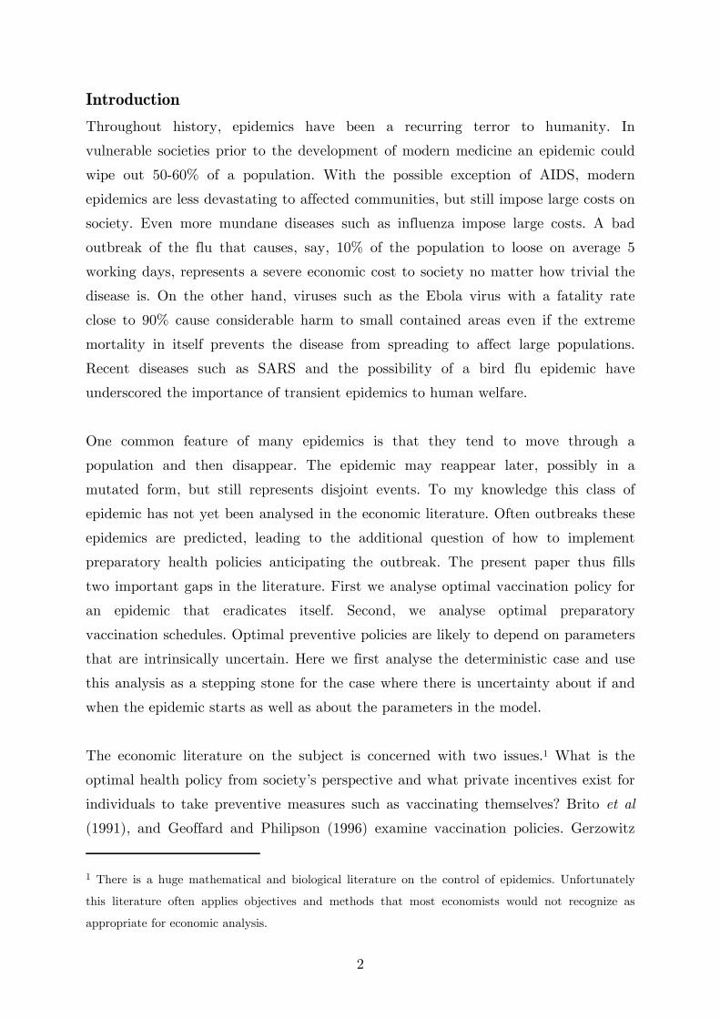
In Figure 8 we have shown the same graph except that β has been changed to 2.7
and c has been changed to 2. Thus we have made the disease slightly less contagious
and the cost of vaccination has increased. The effect on sick days remain monotonic.
More individuals vaccinated at the time of outbreak, implies fewer sick days. But the
effect of pre-outbreak vaccination on vaccination rates after outbreak is dramatically
changed. As the number of vaccinated prior to outbreak increases as from 0 to 0.1,
the number of vaccinated after an outbreak also increases.
Figure 8, Sick days and vaccination rates as a function of x(T*), β = 2.7, c = 2.
This may seem paradoxical. After all, the larger the number of non-vaccinated at the
time of outbreak, the larger is the pool of people there is to vaccinate when the
12

epidemic starts. In order to understand this paradox, one can examine the shadow
price evaluated at the start of the epidemic as a function of the number of vaccinated
at the time of the outbreak. Formally this implies graphing px(T*) as a function of
z(0). This is done in Figure 9.
Figure 9. Shadow price on x(T*) as a function of z(T*)
As expected the shadow price on x is close to zero for low numbers of susceptibles at
time T*. But note that px(x(T*)) is not monotonous. For values of z(T*) ≤ 0.1,
px(x(T*)) is increasing, although still negative. This has an interesting economic
interpretation. Let ϑ(z(T*)) be the value of the objective function when the epidemic
starts at time T*. From well-known theorems in optimal control theory, (see
Seierstad & Sydsæter (1987) pp. 210) it holds that ϑ’(z(T*)) = –px(x(T*)). As the
consequences of the epidemic becomes negligible as z(T*) approaches zero, we have
that limz(T*) → 1ϑ(z(T*)) = 0. With this information we can draw ϑ(z(T*)) as a
function of z(T*) as in Figure 10.
13

Figure 10, The objective function ϑ(z(T*)) as a function of z(T*).
An important aspect of Figure 10 is that as x(T*) is reduced from 1 there is an
initial interval where there are increasing returns to reducing x(T*) and increasing
z(T*). The returns to decreasing the number of susceptibles are increasing, but only
up to a point, indicated by z , where returns to vaccination are positive but
decreasing. As x(T*) → 0, the returns to further reduction go to 0. In our numerical
example, one can see that for low values of x(T*) the return to decreasing x(T*) is
insignificantly different from zero. This fits with the result for the case where there
was no vaccination. With no vaccination there was a threshold x = γ/β such that if
the number of susceptibles at time T* was less than γ/β the epidemic would
immediately fizzle out. Obviously these two facts are related. It simply does not pay
much to sustain a major vaccination program if the number of susceptibles is so low
that the epidemic will burn immediately itself out. Conversely for high values of
x(T*) the increasing returns to reducing the stock of susceptibles imply that if it is
optimal to reduce the number of susceptibles marginally below n, it does in fact pay
to reduce the a significant proportion of the population.
It should be noted that the “brush fire” effect of increasing returns only makes itself
felt for epidemic of relatively low importance. This is shown in Figure 11 where
px(x(T*)) is plotted for different values of w. For low values of w, the p(x(T*)) is
initially decreasing indicating an interval of increasing returns. For high values of w
p(x(T*)) is strictly increasing indicating diminishing returns.
14

Figure 11, Shadow price on susceptibles at time of outbreak with varying costs of disease.
This result is rather counter intuitive as in general one expects increasing returns to
turn up in relatively important problems. There are some strange effects of reducing
the number of susceptibles at the time of the outbreak. For low cost epidemics, the
optimal vaccination schedule implies that the higher the number of initially
susceptible, then, up to a point, the longer is the duration of the epidemic.
0 0.1 0.2 0.3 0.4 0.5 0.6 0.7 0.8 0.9 10
1
2
3
4
5
6
7
8
9
Initial Stock of Vaccinated
Dur
atio
n
w = 0.1w = 0.2w = 0.3
Figure 12, Duration of epidemic as a function of number of vaccinated at time = T*
The reason for this is the same brush fire effect. For high values of x(T*) the disease
spreads so rapidly that one runs through the number of susceptibles quite rapidly. A
relatively large number of individuals are infected quickly, and since as they recover
15
early, the disease burns itself out faster. So even if the number of lost sick days is
larger for higher values of x(T*), they are concentrated in a shorter time interval. If
the cost of disease is high, then we get a picture more in line with intuition in that
epidemic duration is a decreasing function of the number of initially vaccinated. It
interesting to note that optimal vaccination policies accommodate this brush fire
effect for sufficiently high values of x(T*). One way of thinking about this is that
when the number of susceptibles is high enough it pays more to, relatively speaking,
roll with the epidemic punch rather than fight it, until at such time x(t) has
decreased enough to mandate a relatively more aggressive vaccination program.
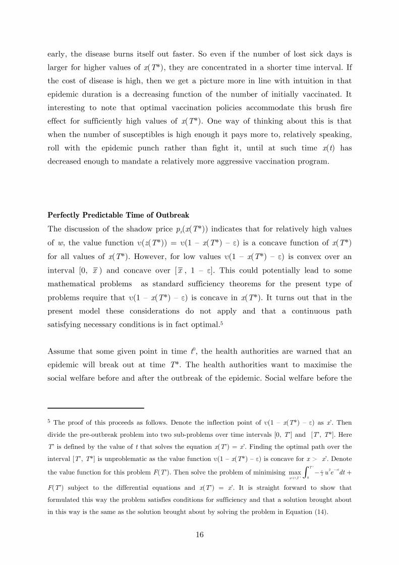
Perfectly Predictable Time of Outbreak
The discussion of the shadow price px(x(T*)) indicates that for relatively high values
of w, the value function υ(z(T*)) = υ(1 – x(T*) – ε) is a concave function of x(T*)
for all values of x(T*). However, for low values υ(1 – x(T*) – ε) is convex over an
interval [0, x ) and concave over [x , 1 – ε]. This could potentially lead to some
mathematical problems as standard sufficiency theorems for the present type of
problems require that υ(1 – x(T*) – ε) is concave in x(T*). It turns out that in the
present model these considerations do not apply and that a continuous path
satisfying necessary conditions is in fact optimal.5
Assume that some given point in time t0, the health authorities are warned that an
epidemic will break out at time T*. The health authorities want to maximise the
social welfare before and after the outbreak of the epidemic. Social welfare before the
5 The proof of this proceeds as follows. Denote the inflection point of υ(1 – x(T*) – ε) as x’. Then
divide the pre-outbreak problem into two sub-problems over time intervals [0, T’] and [T’, T*]. Here
T’ is defined by the value of t that solves the equation x(T’) = x’. Finding the optimal path over the
interval [T’, T*] is unproblematic as the value function υ(1 – x(T*) – ε) is concave for x > x’. Denote
the value function for this problem F(T’). Then solve the problem of minimising ( )
'2
20, '
maxT
rtc
u t Tu e dt−−∫ +
F(T’) subject to the differential equations and x(T’) = x’. It is straight forward to show that
formulated this way the problem satisfies conditions for sufficiency and that a solution brought about
in this way is the same as the solution brought about by solving the problem in Equation (14).
16

epidemic breaks outs is simply total vaccination costs multiplied by -1. The optimal
program to be solved is then:
( ) ( )( )0
*2
2max 1 *T
rtcu t
u e x T−− + υ − − ε∫ (14)
subject to x u= − , x(t0) = n = 1 and u ≥ 0. Let λ be the co-state to the stock of
susceptibles. Applying the appropriate Maximum Principle to this problem gives the
following necessary conditions.
rtx u ecλ= − = (15)
( )( )( )
( )( ) *1 *
0, * **
rTx
x TT
x T−∂υ − − ε
λ = λ = =∂
p T e (16)
From equations (15) and (16) a few observations are obvious. The co-state λ is a
constant over time. This implies that the number of vaccinated increases with the
interest rate through time. Also, the number of susceptibles decreases at the rate of
the interest rate through time. In our numerical example r = 0, so the vaccination
rate is a constant for all t ∈ [t0, T*]. It is a straightforward procedure to solve this
problem numerically as long as px(T*) is known. Since px(T*) is already calculated for
a number of data points (see Figure 5) one can establish a continuous function px(T*)
by using standard interpolation techniques.
The optimal pre-outbreak vaccination schedule obviously depends on the parameters
in the model. One of the important parameters is the amount of time that is
available before an outbreak, that is ∆ = T*- t0. In Figure 9 the number of
susceptibles are plotted for several values of ∆. Since x u= − , the optimal
vaccination schedule is simply the absolute value of the slope of x(t) in Figure 13. It
should be clear from Figure 13 that the larger the value of ∆, the lower is the number
of susceptibles at the time of the outbreak. It does however appear that there are
diminishing returns to increasing ∆. Even if x(T*) is a decreasing function of ∆ the
reduction in x(T*) becomes smaller as ∆ becomes larger. This makes economic sense.
Remember from Figure 5 that px rapidly increased to zero as x(T*) got close to 1.
This was because x(T*) < 1 implied that the epidemic would die out quickly as long
as x(T*) was below the critical threshold. Obviously, as ∆ becomes larger, it pays to
17
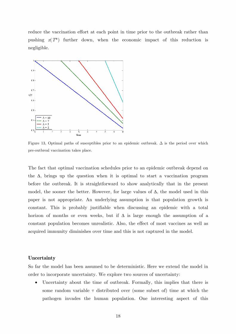
reduce the vaccination effort at each point in time prior to the outbreak rather than
pushing x(T*) further down, when the economic impact of this reduction is
negligible.
Figure 13, Optimal paths of susceptibles prior to an epidemic outbreak. ∆ is the period over which
pre-outbreal vaccination takes place.
The fact that optimal vaccination schedules prior to an epidemic outbreak depend on
the ∆, brings up the question when it is optimal to start a vaccination program
before the outbreak. It is straightforward to show analytically that in the present
model, the sooner the better. However, for large values of ∆, the model used in this
paper is not appropriate. An underlying assumption is that population growth is
constant. This is probably justifiable when discussing an epidemic with a total
horizon of months or even weeks, but if ∆ is large enough the assumption of a
constant population becomes unrealistic. Also, the effect of most vaccines as well as
acquired immunity diminishes over time and this is not captured in the model.
Uncertainty So far the model has been assumed to be deterministic. Here we extend the model in
order to incorporate uncertainty. We explore two sources of uncertainty:
• Uncertainty about the time of outbreak. Formally, this implies that there is
some random variable τ distributed over (some subset of) time at which the
pathogen invades the human population. One interesting aspect of this
18

uncertainty is that for some diseases one can safely assume that the disease
will with probability 1 have an outbreak at some time in the future. The
probability that there will be a new influenza epidemic in the future is close to
one (conditional on the continued existence of the human race.) However,
some epidemic threats may fail to materialize e.g. as they do not make the
jump from animal populations into the human population. Also, some regions
may be unaffected by epidemics even if neighbouring areas are affected.
• Uncertainty about parameters that affect the solution after the outbreak.
Rarely are the parameters affecting the spread of the disease known prior to
an outbreak. Each variety of pathogen has its own properties that can only be
ascertained after the out break. Further, the economic impact of the disease,
here captured by the parameter w, will generally not be know until after the
outbreak.
To keep the presentation brief both types of uncertainty are simultaneously brought
into the model. For illustration purposes we assume that the uncertainty about the
time of outbreak is captured by a quadratic hazard rate φ(t) = at – bt2 defined over
[0, b/a]. This assumption implies that there is a risk of outbreak over the time
interval [0, b/a]. If the epidemic fails to materialize in this time span the probability
of outbreak thereafter is zero.6 It is worthwhile to recall the definition of the hazard
rate. Roughly speaking φ(t) is the probability of τ occurring over some interval [t, t
+ dt] conditional on the event not having occurred at time t. The quadratic form
implies that risk is initially increasing and then decreasing.
The parametric uncertainty affects the optimal vaccination program prior to an
outbreak through the effect on υ(1 – x(τ) – ε). Here x(τ) is the stock of susceptible
individuals at the time of outbreak. To indicate that υ(1 – x(τ) – ε) now depends on
a vector of random variables we write υ(1 – x(τ) – ε) as ω(1 – x(τ) – ε, ξ) where ξ is
a realisation of [γ β w] distributed with a pdf h(ξ) over some set B ⊂ . The
expected value of ω is then given by:
3R
6 It can be shown that in order for φ(t) to be generated by a proper pdf, we must require that b ≤
a√(3/2).
19

( )( ) ( )( ) ( )
( )( )( )
( )( ) ( ) ( )( ) ( )
1 , with
1 , ,
B
xB B
W x w x h d
dW x w x h d p x h ddx
τ = − τ − ε
⎛ ⎞⎟⎜ ⎟′ ⎜τ = − τ − ε = τ⎟⎜ ⎟⎟τ ⎜⎝ ⎠
∫
∫ ∫
ξ ξ ξ
ξ ξ ξ ξ ξ ξ (17)
Having defined W(⋅) and its derivative W’(⋅), we can proceed to state the
optimization problem for pre-outbreak vaccination schedules. The problem can be
stated as follows:
( )( ) ( )( )
( )
( )( )( )
22
0
2
max
, 0 0,
for 0Pr , |
0 elsewhere
ab
rt rcu t
E u e dt W x e
x u x
aat bt dt t bt t dt t
− − τ⎛ ⎞⎟⎜ ⎟⎜ − + τ ⎟⎜ ⎟⎟⎜⎝ ⎠
= − =
⎧⎪ − ≤⎪⎪τ ∈ + τ > ≈ ⎨⎪⎪⎪⎩
∫
≤
(18)
Note that the problem is only solved for the interval [0, a/b] as after t = a/b the risk
has vanished. General necessary conditions for this type of problem can be found in
For ease of reference they are reproduced in the appendix. Applying these conditions
to the problem at hand yields the following conditions:
max 0, rtuc
−µ e⎡ ⎤= −⎢ ⎥⎢ ⎥⎣ ⎦ (19)
( ) ( )( )( ) ( )2 ,rt aat bt W x t e b−′µ = − µ − µ = 0 (20)
Figure 14, Optimal paths when w and time of outbreak are stochastic
20
The resulting paths are shown in Figure 14. As is to be expected, vaccination rates
fall with time. There is an initial period where vaccination rates are relatively high
reflecting that it pays to prepare by vaccinating as risk is increasing. As time
progresses, the need for vaccination decreases as the risk decreases and the
consequences of an outbreak decreases.
Summary and Conclusions The present paper has analysed a class of epidemics not previously analysed in the
literature. A model that defines optimal vaccination schedules before and after an
outbreak of an epidemic has been identified. Numerical methods have been used to
solve the model and general properties of optimal vaccination schedules have been
inferred from studying the resulting paths.
21

References:
Ascher, U. M. and L. R. Petzold, (1998), Computer Methods for Ordinary
Differential Equations and Differential-Algebraic Equations, Society for Industrial
and Applied Mathematics.
Barrett S. and M. Hoel (2003), Optimal Disease Eradication, HERO on-line working
paper series, University of Oslo, 2003:23. (Forthcoming in Environment and
Development Economics.)
http://www.hero.uio.no/publicat/2003/HERO2003_23.pdf
Brito D. L., E. Sheshinski and M. D. Intriligator, (1991). Externalities and
compulsary vaccinations, Journal of Public Economics, 45, 1,:69-90.
Geoffard P.-Y., T. Philipson, (1996). Rational Epidemics and Their Public Control,
International Economic Review, 37, 3:603-624.
Gersovitz, M. and J.S. Hammer, (2004). The Economical Control of Infectious
Diseases, The Economic Journal, 114, 492:1–27.
Goldman S.M. and J. Lightwood (2002), Cost Optimization in the SIS Model of
Infectious Disease with Treatment, Topics in Economic Analysis & Policy, 2, 1,
Article 4.
Kermac, W.O. and A.G. McKendrick, (1927). A Mathematical Theory of Epidemics,
Proceedings of the Royal Society of London, 115, 700–721, 1927.
Laxminarayan, R and G. M. Brown, (2000), Economics of Antibiotic Resistance: A
Theory of Optimal Use, Journal of Environmental Economics and Management, 42,
2:183-206.
Luenberger, D. G., Introduction to Dynamic Systems, John Wiley & Sons, 1979.
Nævdal, E., (2003), Numerical Continuous Time Optimal Control Problems with a
Spreadsheet, Journal of Economic Education, 34, 2:99–122.
22

Nævdal, E., (2002), Solving Optimal Control in Continuous Time Made Easy,
Computers in Higher Economic Education, 16, 1:8–15.
Seierstad, A. and K. Sydsæter, Optimal Control Theory with Economic Applications,
North Holland, 1987.
23

Appendix - Piecewise Deterministic Optimal Control of Poisson
Processes. This appendix presents necessary conditions for Piecewise Deterministic Optimal
Control problems. The conditions presented here are due to Seierstad (2003).
Although alternative, but equivalent, formulations exist in the literature this method
is to my knowledge the most general. In addition, this formulation has two
advantages that other formulations do not have.
1. The Hamiltonian and co-state variables have interpretations that are equivalent
to the interpretation of these quantities in deterministic control theory.
2. The necessary conditions often take the form of autonomous differential equations.
This facilitates steady state analysis.
The general problem to be studied is:
( )( ) ( ) ( )( )( )0
0, 0 max , rt r
u UJ x E f x u e dt x e
τ−
∈= + υ τ − τ∫ (A.1)
( ) ( ). : , 0 , ,m ns t u x x g x u⊆ ⊆ =R R (A.2)
(A.3) ( )( )
0~ over t
dt e
− λ σ σ∫τ λ ∞[0, )
Here τ is the time dependent hazard rate. If the event τ occurs at some point in time,
the problem ends with some payoff . ( )( ), rx e− τυ τ ξ ( )( ), rx e− τυ τ ξ can be interpreted
as the solution to a deterministic optimal control problem that starts after the event
has occurred. ξ is a vector of random variables which become known at time τ. All
functions are assumed to be twice differentiable.
( ) ( ), rtH f x u e g x u−= + µ ,
),
)
(A.4)
This Hamiltonian differs from the Hamiltonian from deterministic control theory only
by the term λ(x)( ). J(t, x) is defined by the solution to
problem:
( )( ) (, |J t x q x t J t x+ τ = −
( ) ( ) ( )(, max ,T
r s t
u U tJ t x E f y u e ds− −
∈= ∫ (A.5)
24

( ) ( ). : , , ,m ns t u y t x y g y u⊆ = ⊆ =R R (A.6)
( )( )( )( )
0~ ov s
x dx s e t
− λ ζ ζer [ , )∫σ λ ∞ (A.7)
(A.8) ( ) ( ) ( )(x x q x+ −σ − σ = σ )−
)
This problem is exactly the same as the problem posed in Equations (A.1) -
Error! Reference source not found. except that the problem starts from an arbitrary
point (t, x). J(t, x) is thus the value to the objective function when the problem
starts from some arbitrary point in (t, x) space. The term is defined by: ( , |J t y tτ =
( ) ( ) ( ), | max ,T
r s t
u U tJ t x t f y u e ds− −
∈τ = = ∫ (A.9)
(A.10) (. : , , ,m ns t u x y g y u⊆ ⊆ =R R )
)) )
)
),
H
This problem differs from the one posed in Equations (A.1) -
Error! Reference source not found. in two respects. The problem is a deterministic
problem and the starting point is an arbitrary point in (t, x) space after the shock
has happened. In order to solve the problem in equation (A.1) one must find a
solution to (A.9). The solution to (A.9) will be a function , a control
and a co-state . It is clear that J(t, x |τ = t) =
is the value of criterion after a shock has driven the
system to some arbitrary state x at time t. J(t, x |τ = t) is thus the criterion
conditional on the event τ occurring at time t. The interpretation of
should now be clear. It is the net loss (or gain) to the
objective system if the shock occurs at an arbitrary point in time t and results in the
state variable taking the value x. Now apply the maximum principle to the
Hamiltonian in (A.4). Doing so yields the following conditions:
( | ,y s t x
( | ,u s t x ( | ,s t xµ
( ) ( )( | , , | , rs
tf y s t x u s t x e ds
∞−∫
( )( ) ( )( , |J t x q x J t x+ τ −
(A.11) ( )argmaxy
u =
( ) ( )
( ) ( ) ( )( ) ( ) ( ) ( )( )( )
, ,
, , | , ,
x xHr r f x u g x ux
x J t x J t x q x x J t x J t x q xx x
∂ ′ ′µ = µ − = µ − − µ +∂
⎛ ⎞∂ ∂ ⎟⎜ ′λ − + τ + λ − + τ⎟⎜ ⎟⎜⎝ ⎠∂ ∂|
(A.12)
Coupled with the appropriate transversality condition, the solution is determined by
the equation for x , (A.16) and (A.17). It follows from standard results in
deterministic control theory that:
25

( )( ) ( )( )(, , | | , nxJ t x q t x t t x q x I q
x∂ ′+ τ = µ + +∂
) (A.13)
Here In is the n-dimensional identity matrix. The final piece of information required
to solve the problem in (A.1) is an expression for J(t, x), as this expression and an
expression for ( )( ),x J t x∂∂ are needed in order to solve (A.12).
To find an expression for J(t, x), define the following differential equation:
(A.14) ( ) ( ) ( )((, ,z rz f x u x z J t x q t x= − + λ − + )),
The solution to (A.14) is a function z(t) that is equal to J(t, x(t)) along the optimal
path. Seierstad (2003) has proven that:
( ) ( ),J t x tx∂ = µ∂
(A.15)
Rewriting (A.16) and (A.17), using (A.13), (A.15) and exchanging J(t, x) with z
gives:
(A.16) ( ) ( ) ( ) ( )(( )( )argmax , , , , |y
u f x u g x u x J t x q t x= + µ + λ + τ −) z
( ) ( )
( ) ( )( )( )( ) ( ) ( )( )( )
, ,
| , , |
x x
nx
Hr r f x u g x ux
x t t x q x I q x J t x q x t z
∂ ′ ′µ = µ − = µ − − µ −∂
′ ′λ µ + + − µ −λ + τ = − (A.17)
The differential equations in (A.14), (A.16), (A.17) and the differential equation x =
f(x, u) gives the necessary conditions required to solve the problem at hand when
coupled to the appropriate transversality conditions. For the case where T < ∞, the
transversality conditions are given by:
( ) 0Tµ = (A.18)
( ) 0z T = (A.19)
Equation (A.18) is the transversality condition on the co-state. Paralleling the
interpretation of the co-state variable in the deterministic problem, the interpretation
26
is that at the end of the planning horizon, the marginal value of x is zero in the
absence of any scrap value. The condition that z(T) = 0, is best understood by
noting from the definition of z(t) that z(T) = J(T, x(T)). Thus, z(T) is the
“remaining” utility to be consumed at the end of the planning horizon and equal to
zero. If T = ∞, then as long as instantaneous utility is bounded, the following
conditions will usually work and be consistent with Catching Up Optimality. If x is
the optimal path, then for all admissible paths y satisfying u ∈ U and y = g(y, u).
( ) ( )( )lim 0rt
te y t x t−
→∞µ − ≥ (A.20)
(A.21) ( )lim 0rt
tz t e−
→∞=
These conditions are required to take care of some special cases that turn up in
infinite horizon models. These conditions may often be replaced by µ(∞) = z(∞) =
0. In particular, this is the case if the steady state is unique.7 If the limit in equation
(A.20) does not exist, which will only be the case in very rare problems, the lim
operator must be replaced by lim inf.
7The issues involved here are parallel to the problems encountered in deterministic control theory. See
Seierstad and Sydsæter (1987), pp 229-250.
27
Top Related