


Languages
Pages
Legal


Chapter 2 - Frequency Distributions and Graphs
3
EXERCISE SET 2-1
1. Frequency distributions are used toorganize data in a meaningful way, tofacilitate computational procedures forstatistics, to make it easier to draw chartsand graphs, and to make comparisons amongdifferent sets of data.
2. Categorical distributions are used withnominal or ordinal data, ungroupeddistributions are used with data having asmall range, and grouped distributions areused when the range of the data is large.
3.
a. 31.5 38.5 35 ß œ œ ß$#$) (!# #
38.5 31.5 œ (
b. 85.5 104.5 95 ß œ œ ß)'"!% "*!# #
104.5 85.5 œ "*
c. 894.5 905.5 900 ß œ œ ß)*&*!& ")!!# #
905.5 894.5 œ ""
d. 12.25 13.55 12.9 ß œ œ ß"#Þ$ "$Þ& #&Þ)# #
13.55 12.25 1.3 œ
e. 3.175 4.965 4.07 ß œ œ ß$Þ") %Þ*' )Þ"%# #
4.965 3.175 1.79 œ
4. Five to twenty classes. Width should bean odd number so that the midpoint willhave the same place value as the data.
5.a. Class width is not uniform.b. Class limits overlap, and class width isnot uniform.c. A class has been omitted.d. Class width is not uniform.
6. An open-ended frequency distribution haseither a first class with no lower limit or alast class with no upper limit. They arenecessary to accomodate all the data.
7.
A 4 10%
M 28 70%
H 6 15%
S 2 5%
40 100%
Class Tally f Percent
8. H 52 L 21œ œRange 52 21 31œ œ
8. continuedWidth 31 5 6.2 or 7œ ƒ œ
Limits Boundaries f
21 - 27 20.5 - 27.5 6
28 - 34 27.5 - 34.5 9
35 - 41 34.5 - 41.5 5
42 - 48 41.5 - 48.5 7
49 - 55 48.5 - 55.5
30
3
cf
Less than 20.5 0
Less than 27.5 6
Less than 34.5 15
Less than 41.5 20
Less than 48.5 27
Less than 55.5 30
9. H 325 L 165œ œRange 325 165 160œ œWidth 160 8 20 round up to 21œ ƒ œ
Limits Boundaries f
165 - 185 164.5 - 185.5 4
186 - 206 185.5 - 206.5 6
207 - 227 206.5 - 227.5 15
228 - 248 227.5 - 248.5 13
249 - 269 248.5 - 269.5 9
270 - 290 269.5 - 290.5 1
291 - 311 290.5 - 311.5 1
312 - 332 311.5 - 332.5 1
50
A peak occurs in class 207 - 227. There areno empty classes. Each of the three highestclasses has one data value.
cf
Less than 164.5 0
Less than 185.5 4
Less than 206.5 10
Less than 227.5 25
Less than 248.5 38
Less than 269.5 47
Less than 290.5 48
Less than 311.5 49
Less than 332.5 50
10. H 110 L 54œ œRange 110 54 56œ œWidth 56 7 8 round up to 9œ ƒ œ
Elementary Statistics A Step by Step Approach 8th Edition Bluman Solutions ManualFull Download: http://alibabadownload.com/product/elementary-statistics-a-step-by-step-approach-8th-edition-bluman-solutions-manual/
This sample only, Download all chapters at: alibabadownload.com

Chapter 2 - Frequency Distributions and Graphs
4
10. continuedLimits Boundaries f
54 - 62 53.5 - 62.5 7
63 - 71 62.5 - 71.5 6
72 - 80 71.5 - 80.5 8
81 - 89 80.5 - 89.5 4
90 - 98 89.5 - 98.5 1
99 - 107 98.5 - 107.5 3
108 - 116 107.5 - 116.5
30
1
cf
Less than 53.5 0
Less than 62.5 7
Less than 71.5 13
Less than 80.5 21
Less than 89.5 25
Less than 98.5 26
Less than 107.5 29
Less than 116.5 30
11. H 780 L 746œ œRange 780 746 34œ œWidth 34 5 6.8 round up to 7œ ƒ œ
Limits Boundaries f
746 - 752 745.5 - 752.5 4
753 - 759 752.5 - 759.5 6
760 - 766 759.5 - 766.5 8
767 - 773 766.5 - 773.5 9
774 - 780 773.5 - 780.5
30
3
cf
Less than 745.5 0
Less than 752.5 4
Less than 759.5 10
Less than 766.5 18
Less than 773.5 27
Less than 780.5 30
12. H 91,570 L 5427œ œRange 91,570 5427 86,143œ œWidth 86,143 7 12,306.1œ ƒ œRound up to 12,307
12. continuedLimits Boundaries f
5427 - 17,733 5426.5 - 17,733.5 17
17,734 - 30,040 17,733.5 - 30,040.5 1
30,041 - 42,347 30,040.5 - 42,347.5 1
42,348 - 54,654 42,347.5 - 54,654.5 1
54,655 - 66,961 54,654.5 - 66,961.5 1
66,962 - 79,268 66,961.5 - 79,268.5 1
79,269 - 91,575 79,268.5 - 91,575.5 3
25
The majority of the data values are in thelowest class. There are no empty classes inthe distribution.
cf
Less than 5426.5 0
Less than 17,733.5 17
Less than 30,040.5 18
Less than 42,347.5 19
Less than 54,654.5 20
Less than 66,961.5 21
Less than 79,268.5 22
Less than 91,575.5 25
13. H 70 L 27œ œRange 70 27 43œ œWidth 43 7 6.1 or 7œ ƒ œ
Limits Boundaries f
27 - 33 26.5 - 33.5 7
34 - 40 33.5 - 40.5 14
41 - 47 40.5 - 47.5 15
48 - 54 47.5 - 54.5 11
55 - 61 54.5 - 61.5 3
62 - 68 61.5 - 68.5 3
69 - 75 68.5 - 75.5
55
2
cf
Less than 26.5 0
Less than 33.5 7
Less than 40.5 21
Less than 47.5 36
Less than 54.5 47
Less than 61.5 50
Less than 68.5 53
Less than 75.5 55
14. H 51.7 L 1.2œ œRange 51.7 1.2 50.5œ œWidth 50.5 5 10.1 round up to 11œ ƒ œ
Chapter 2 - Frequency Distributions and Graphs
5
14. continuedLimits Boundaries f
0 - 10 -0.5 - 10.5 7
11 - 21 10.5 - 21.5 6
22 - 32 21.5 - 32.5 2
33 - 43 32.5 - 43.5 0
44 - 54 43.5 - 54.5
16
1
cf
Less than -0.5 0
Less than 10.5 7
Less than 21.5 13
Less than 32.5 15
Less than 43.5 15
Less than 54.5 16
15. H 635 L 6œ œWidth 635 6 629œ œRange 629 5 125.8 round up to 127œ ƒ œ
Limits Boundaries f
6 - 132 5.5 - 132.5 16
133 - 259 132.5 - 259.5 3
260 - 386 259.5 - 386.5 0
387 - 513 386.5 - 513.5 0
514 - 640 513.5 - 640.5
20
1
The greatest concentration of data values isin the lowest class. All but one of the datavalues are in the lowest two classes. Thereis one extremely large data value occurringin the highest class.
cf
Less than 5.5 0
Less than 132.5 16
Less than 259.5 19
Less than 386.5 19
Less than 513.5 19
Less than 640.5 20
16. H 857 L 140œ œWidth 857 140 717œ œRange 717 8 89.6 or 91œ ƒ œ
16. continuedLimits Boundaries f
140 - 230 139.5 - 229.5 11
231 - 321 230.5 - 321.5 5
322 - 412 321.5 - 412.5 4
413 - 503 412.5 - 503.5 4
504 - 594 503.5 - 594.5 4
595 - 685 594.5 - 685.5 1
686 - 776 685.5 - 776.5 0
777 - 867 776.5 - 867.5
30
1
cf
Less than 139.5 0
Less than 229.5 11
Less than 321.5 16
Less than 412.5 20
Less than 503.5 24
Less than 594.5 28
Less than 685.5 29
Less than 776.5 29
Less than 867.5 30
17. H 123 L 77œ œRange 123 77 46œ œWidth 46 7 6.6 or 7œ ƒ œ
Limits Boundaries f
77 - 83 76.5 - 83.5 1
84 - 90 83.5- 90.5 1
91 - 97 90.5- 97.5 6
98 - 104 97.5- 104.5 14
105 - 111 104.5 - 111.5 8
112 - 118 111.5 - 118.5 1
119 - 125 118.5 - 125.5
32
1
cf
Less than 76.5 0
Less than 83.5 1
Less than 90.5 2
Less than 97.5 8
Less than 104.5 22
Less than 111.5 30
Less than 118.5 31
Less than 125.5 32
18.H 31.5 L 7.5œ œRange 31.5 7.5 24œ œWidth 24 5 4.8 or 5œ ƒ œ

Chapter 2 - Frequency Distributions and Graphs
6
18. continuedLimits Boundaries f
7.5 - 12.4 7.45 - 12.45 1
12.5 - 17.4 12.45 - 17.45 4
17.5 - 22.4 17.45 - 22.45 10
22.5 - 27.4 22.45 - 27.45 6
27.5 - 32.4 27.45 - 32.45
25
4
cf
Less than 7.45 0
Less than 12.45 1
Less than 17.45 5
Less than 22.45 15
Less than 27.45 21
Less than 32.45 25
19. The percents add up to 101%. Theyshould total 100% unless rounding was used.
EXERCISE SET 2-2
1.
0
1020
3040
50
89.5-
98.5
98.5-
107.5
107.5-
116.5
116.5-
125.5
125.5-
134.5
I.Q.
fre
qu
en
cy
0
20
40
60
85 94 103 112 121 130 139
I.Q.
fre
qu
en
cy
0
20
40
60
80
100
120
89.5 98.5 107.5 116.5 125.5 134.5
I.Q.
cu
mu
lati
ve f
req
uen
cy
Eighty applicants do not need to enroll in thesummer programs.
2.Limits Boundaries f
70 - 116 69.5 - 116.5 5
117 - 163 116.5 - 163.5 9
164 - 210 163.5 - 210.5 6
211 - 257 210.5 - 257.5 6
258 - 304 257.5 - 304.5 0
305 - 351 304.5 - 351.5 1
352 - 398 351.5 - 398.5
28
1
cf
Less than 69.5 0
Less than 116.5 5
Less than 163.5 14
Less than 210.5 20
Less than 257.5 26
Less than 304.5 26
Less than 351.5 27
Less than 398.5 28
0
2
4
6
8
10
69.5-116.5 116.5-163.5 163.5-210.5 210.5-257.5 257.5-304.5 304.5-351.5 351.5-398.5
Number of faculty
0
2
4
6
8
10
93 140 187 234 281 328 375
Number of faculty
freq
uen
cy
0
5
10
15
20
25
30
69.5 116.5 163.5 210.5 257.5 304.5 351.5 398.5
Number of faculty
cu
mu
lati
ve
fre
qu
en
cy
"##)
œ 0.429 or 42.9% have 180 or more.
The histogram and frequency polygon arepositively skewed.

Chapter 2 - Frequency Distributions and Graphs
7
3.Limits Boundaries f
3 - 45 2.5 - 45.5 19
46 - 88 45.5 - 88.5 19
89 - 131 88.5 - 131.5 10
132 - 174 131.5 - 174.5 1
175 - 217 174.5 - 217.5 0
218 - 260 217.5 - 260.5
50
1
cf
Less than 2.5 0
Less than 45.5 19
Less than 88.5 38
Less than 131.5 48
Less than 174.5 49
Less than 217.5 49
Less than 260.5 50
0
5
10
15
20
2.5-45.5 45.5-88.5 88.5-131.5 131.5-174.5 174.5-217.5 217.5-260.5
Counties, parishes, or divisions
freq
uen
cy
The distribution is positively skewed.
0
5
10
15
20
24 67 110 153 196 239
Counties, parishes, or divisions
fre
qu
en
cy
0
10
20
30
40
50
60
2.5 45.5 88.5 131.5 174.5 217.5 260.5
Counties, parishes, or divisions
cu
mu
lati
ve
fre
qu
en
cy
4.
0
2
4
6
8
10
12
14
39.85-42.85 42.85-45.85 45.85-48.85 48.85-51.85 51.85-54.85 54.85-57.85
Millions of Dollars
freq
uen
cy
0
2
4
6
8
10
12
14
38.35 41.35 44.35 47.35 50.35 53.35 56.35 59.35
Millions of Dollars
fre
qu
en
cy
0
5
10
15
20
25
30
35
38.85 42.85 45.85 48.85 51.85 54.85 57.85
Millions of Dollars
cu
mu
lati
ve f
req
uen
cy
The distribution is left skewed or negativelyskewed.
5.Limits Boundaries f
1 - 43 0.5 - 43.5 24
44 - 86 43.5 - 86.5 17
87 - 129 86.5 - 129.5 3
130 - 172 129.5 - 172.5 4
173 - 215 172.5 - 215.5 1
216 - 258 215.5 - 258.5 0
259 - 301 258.5 - 301.5 0
302 - 344 301.5 - 344.5
50
1
cf
Less than 0.5 0
Less than 43.5 24
Less than 86.5 41
Less than 129.5 44
Less than 172.5 48
Less than 215.5 49
Less than 258.5 49
Less than 301.5 49
Less than 344.5 50
The distribution is positively skewed.

Chapter 2 - Frequency Distributions and Graphs
8
5. continued
0
5
10
15
20
25
30
0.5-43.5 43.5-86.5 86.5-129.5 129.5-172.5 172.5-215.5 215.5-258.5 258.5-301.5 301.5-344.5
Accidents
Fre
qu
en
cy
0
5
10
15
20
25
30
22 65 108 151 194 237 280 323
Accidents
Fre
qu
en
cy
0
10
20
30
40
50
60
0.5 43.5 86.5 129.5 172.5 215.5 258.5 301.5 344.5
Accide nts
Cu
mu
lati
ve F
req
uen
cy
6.Limits Boundaries f
6 - 8 5.5 - 8.5 12
9 - 11 8.5 - 11.5 16
12 - 14 11.5 - 14.5 3
15 - 17 14.5 - 17.5 1
18 - 20 17.5 - 20.5 0
21 - 23 20.5 - 23.5 0
24 - 26 23.5 - 26.5
33
1
cf
Less than 5.5 0
Less than 8.5 12
Less than 11.5 28
Less than 14.5 31
Less than 17.5 32
Less than 20.5 32
Less than 23.5 32
Less than 26.5 33
The distribution is positively skewed.
6. continued
0
5
10
15
20
5.5-8.5 8.5-11.5 11.5-14.5 14.5-17.5 17.5-20.5 20.5-23.5 23.5-26.5
Costs of utilities
Fre
qu
en
cy
0
5
10
15
20
7 10 13 16 19 22 25
Costs of utilities
Fre
qu
en
cy
0
5
10
15
20
25
30
35
5.5 8.5 11.5 14.5 17.5 20.5 23.5 26.5
Costs of utilities
Cu
mu
lati
ve f
req
uen
cy
7.Limits Boundaries f f (1998) (2003)
0 - 22 -0.5 - 22.5 18 26
23 - 45 22.5 - 45.5 7 1
46 - 68 45.5 - 68.5 3 0
69 - 91 68.5 - 91.5 1 1
92 - 114 91.5 - 114.5 1 0
115 - 137 114.5 - 137.5 0 1
138 - 160 137.5 - 160.5
30 30
0 1

Chapter 2 - Frequency Distributions and Graphs
9
7. continued
0
5
10
15
20
-0.5-
22.5
22.5-
45.5
45.5-
68.5
68.5-
91.5
91.5-
114.5
114.5-
137.5
137.5-
160.5
Days 1998
freq
uen
cy
0
5
1015
20
25
30
-0.5-
22.5
22.5-
45.5
45.5-
68.5
68.5-
91.5
91.5-
114.5
114.5-
137.5
137.5-
160.5
Days 2003
freq
uen
cy
Both distributions are positively skewed, butthe data are somewhat more spread out inthe first three classes in 1998 than in 2003.There are two large data values in the 2003data.
8.
02468
1012
2.25-
2.95
2.95-
3.65
3.65-
4.35
4.35-
5.05
5.05-
5.75
5.75-
6.45
Time
fre
qu
en
cy
0
5
10
15
1.9 2.6 3.3 4.0 4.7 5.4 6.1 6.8
Time
fre
qu
en
cy
0
10
20
30
40
50
2.25 2.95 3.65 4.35 5.05 5.75 6.45
Time
cu
mu
lati
ve f
req
uen
cy
The data values fall somewhat on the leftside of the distribution. The histogram isright skewed. There are no gaps in thehistogram.
9.Limits Boundaries f
83.1 - 90.0 83.05 - 90.05 3
90.1 - 97.0 90.05 - 97.05 5
97.1 - 104.0 97.05 - 104.05 6
104.1 - 111.0 104.05 - 111.05 7
111.1 - 118.0 111.05 - 118.05 3
118.1 - 125.0 118.05 - 125.05
25
1
cf
Less than 83.05 0
Less than 90.05 3
Less than 97.05 8
Less than 104.05 14
Less than 111.05 21
Less than 118.05 24
Less than 125.05 25
0
2
4
6
8
83.05-
90.05
90.05-
97.05
97.05-
104.05
104.05-
111.05
111.05-
118.05
118.05-
125.05
Scores
freq
uen
cy
0
2
4
6
8
86.55 93.55 100.55 107.55 114.55 121.55
Scores
freq
uen
cy
0
10
20
30
83.05 90.05 97.05 104.05 111.05 118.05 125.05
Scores
freq
uen
cy
10.
0
5
10
15
20
17.5 -
22.5
22.5 -
27.5
27.5 -
32.5
32.5 -
37.5
37.5 -
42.5
42.5 -
47.5
% At or Above Reading Level
freq
uen
cy

Chapter 2 - Frequency Distributions and Graphs
10
10. continued
0
5
10
15
20
17.5 -
22.5
22.5 -
27.5
27.5 -
32.5
32.5 -
37.5
37.5 -
42.5
42.5 -
47.5
% At or Above Math Level
freq
uen
cy
The distribution of math percentages is morebell-shaped than the distribution of readingpercentages, and its peak in the class of32.5 37.5 is not as high as the peak of thereading percentages.
11.Limits Boundaries f
140 - 230 139.5 - 229.5 11
231 - 321 230.5 - 321.5 5
322 - 412 321.5 - 412.5 4
413 - 503 412.5 - 503.5 4
504 - 594 503.5 - 594.5 4
595 - 685 594.5 - 685.5 1
686 - 776 685.5 - 776.5 0
777 - 867 776.5 - 867.5
30
1
cf
Less than 139.5 0
Less than 229.5 11
Less than 321.5 16
Less than 412.5 20
Less than 503.5 24
Less than 594.5 28
Less than 685.5 29
Less than 776.5 29
Less than 867.5 30
The distribution is positively skewed.
11. continued
0
2
4
6
8
10
12
139.5-
230.5
230.5-
321.5
321.5-
412.5
412.5-
503.5
503.5-
594.5
594.5-
685.5
685.5-
776.5
776.5-
867.5
Unclaimed prizes
Fre
qu
en
cy
0
2
4
6
8
10
12
185 276 367 458 549 640 731 822
Unclaimed prizes
Fre
qu
en
cy
0
5
10
15
20
25
30
35
139.5 230.5 321.5 412.5 503.5 594.5 685.5 776.5 867.5
Unclaimed prizes
Cu
mu
lati
ve f
req
uen
cy
12.
0
2
4
6
8
10
12
7.45-12.45 12.45-17.45 17.45-22.45 22.45-27.45 27.45-32.45
State Gasoline Tax
Fre
qu
en
cy
The histogram shows that state gasolinetaxes are somewhat normal with the peak inthe middle of the graph.
13.
0
0.1
0.2
0.3
0.4
89.5-
98.5
98.5-
107.5
107.5-
116.5
116.5-
125.5
125.5-
134.5
I. Q.
rela
tiv
e f
req
ue
nc
y

Chapter 2 - Frequency Distributions and Graphs
11
13. continued
0
0.1
0.2
0.3
0.4
85 94 103 112 121 130 139
I. Q.
rela
tive f
req
uen
cy
0
0.2
0.4
0.6
0.8
1
89.5 98.5 107.5 116.5 125.5 134.5
I. Q.
cu
mu
lati
ve r
ela
tive
freq
uen
cy
The proportion of applicants who need toenroll in a summer program is 0.26 or 26%.
14.Limits Boundaries rf
1 - 43 0.5 - 43.5 0.48
44 - 86 43.5 - 86.5 0.34
87 - 129 86.5 - 129.5 0.06
130 - 172 129.5 - 172.5 0.08
173 - 215 172.5 - 215.5 0.02
216 - 258 215.5 - 258.5 0
259 - 301 258.5 - 301.5 0
302 - 344 301.5 - 344.5 0.02
crf
Less than 0.5 0
Less than 43.5 0.48
Less than 86.5 0.82
Less than 129.5 0.88
Less than 172.5 0.96
Less than 215.5 0.98
Less than 258.5 0.98
Less than 301.5 0.98
Less than 344.5 1.00
Of the states 82% have fewer than 87accidents per year.
14. continued
0
0.1
0.2
0.3
0.4
0.5
0.6
0.5-43.5 43.5-86.5 86.5-129.5 129.5-172.5 172.5-215.5 215.5-258.5 258.5-301.5 301.5-344.5
Accidents
Fre
qu
en
cy
0
0.1
0.2
0.3
0.4
0.5
0.6
22 65 108 151 194 237 280 323
Accidents
Fre
qu
en
cy
0
0.2
0.4
0.6
0.8
1
1.2
0.5 43.5 86.5 129.5 172.5 215.5 258.5 301.5 344.5
AccidentsC
um
ula
tive f
req
uen
cy
15. H 270 L 80œ œRange 270 80 190œ œWidth 190 7 27.1 or 28œ ƒ œUse width 29 (rule 2)œ
Limits Boundaries f rf
80 - 108 79.5 - 108.5 8 0.17
109 - 137 108.5 - 137.5 13 0.28
138 - 166 137.5 - 166.5 2 0.04
167 - 195 166.5 - 195.5 9 0.20
196 - 224 195.5 - 224.5 10 0.22
225 - 253 224.5 - 253.5 2 0.04
254 - 282 253.5 - 282.5 2
0.99*
0.04
*due to rounding
crf
Less than 79.5 0.00
Less than 108.5 0.17
Less than 137.5 0.45
Less than 166.5 0.49
Less than 195.5 0.69
Less than 224.5 0.91
Less than 253.5 0.95
Less than 282.5 0.99

Chapter 2 - Frequency Distributions and Graphs
12
15. continued
0
0.05
0.1
0.15
0.2
0.25
0.3
79.5-108.5 108.5-137.5 137.5-166.5 166.5-195.5 195.5-224.5 224.5-253.5 153.5-282.5
Calories
rela
tive f
req
uen
cy
0
0.05
0.1
0.15
0.2
0.25
0.3
65 94 123 152 181 210 239 268 297
Calories
rela
tive f
req
uen
cy
0
0.2
0.4
0.6
0.8
1
1.2
79.5 108.5 137.5 166.5 195.5 224.5 253.5 282.5
Calories
cu
mu
lati
ve
re
lati
ve f
req
ue
nc
y
The histogram has two peaks.
16.H 57 L 12œ œRange 57 12 45œ œWidth 45 6 7.5 or 8œ ƒ œ
Limits Boundaries f rf
12 - 19 11.5 - 19.5 7 0.175
20 - 27 19.5 - 27.5 17 0.425
28 - 35 27.5 - 35.5 10 0.25
36 - 43 35.5 - 43.5 4 0.10
44 - 51 43.5 - 51.5 1 0.025
52 - 59 51.5 - 59.5
40 1.000
1 0.025
crf
Less than 11.5 0.000
Less than 19.5 0.175
Less than 27.5 0.600
Less than 35.5 0.850
Less than 43.5 0.950
Less than 51.5 0.975
Less than 59.5 1.000
16. continued
0
0.05
0.1
0.15
0.2
0.25
0.3
0.35
0.4
0.45
11.5-19.5 19.5-27.5 27.5-35.5 35.5-43.5 43.5-51.5 51.5-59.5
Grams
rela
tive f
req
uen
cy
0
0.05
0.1
0.15
0.2
0.25
0.3
0.35
0.4
0.45
7.5 15.5 23.5 31.5 39.5 47.5 55.5 63.5
Grams
rela
tive f
req
uen
cy
0
0.2
0.4
0.6
0.8
1
1.2
11.5 19.5 27.5 35.5 43.5 51.5 59.5
Gramscu
mu
lati
ve
rela
tiv
e
fre
qu
en
cy
The histogram is positively skewed.
17.Boundaries crf
-0.5 - 27.5 0.87
27.5 - 55.5 0.03
55.5 - 83.5 0.00
83.5 - 111.5 0.03
111.5 - 139.5 0.00
139.5 - 167.5 0.03
167.5 - 195.5 0.03
0.99
crf
Less than -0.5 0.00
Less than 27.5 0.87
Less than 55.5 0.90
Less than 83.5 0.90
Less than 111.5 0.93
Less than 139.5 0.93
Less than 167.5 0.96
Less than 195.5 0.99

Chapter 2 - Frequency Distributions and Graphs
13
17. continued
0
0.1
0.2
0.3
0.4
0.5
0.6
0.7
0.8
0.9
1
-0.5-27.5 27.5-55.5 55.5-83.5 83.5-111.5 111.5-139.5 139.5-167.5 137.5-195.5
Air Quality ( Days) - 2003
Fre
qu
en
cy
0
0.2
0.4
0.6
0.8
1
11 34 57 80 103 126 149
Air Quality (Days) - 2003
Fre
qu
en
cy
0
0.2
0.4
0.6
0.8
1
-0.5 27.5 55.5 83.5 111.5 139.5 167.5 195.5
Air Quality (Days) - 2003
Fre
qu
en
cy
18.
0
5
10
15
20
2.25 - 2.95 2.95 - 3.65 3.65 - 4.35 4.35 - 5.05 5.05 - 5.75 5.75 - 6.45
Seconds
fre
qu
en
cy
0
5
10
15
20
2.6 3.3 4 4.7 5.4 6.1
Seconds
fre
qu
en
cy
0
10
20
30
40
50
2.25 2.95 3.65 4.35 5.05 5.75 6.45
Seconds
fre
qu
en
cy
18. continuedBased on the histograms, the older dogshave longer reaction times. Also, thereaction times for older dogs is morevariable.
19.Limits Boundaries X fm
22 - 24 21.5 - 24.5 23 1
25 - 27 24.5 - 27.5 26 3
28 - 30 27.5 - 30.5 29 0
31 - 33 30.5 - 33.5 32 6
34 - 36 33.5 - 36.5 35 5
37 - 39 36.5 - 39.5 38 3
40 - 42 39.5 - 42.5 41
20
2
cf
Less than 21.5 0
Less than 24.5 1
Less than 27.5 4
Less than 30.5 4
Less than 33.5 10
Less than 36.5 15
Less than 39.5 18
Less than 42.5 20
0
2
4
6
8
23 26 29 32 35 38 41
Seconds
fre
qu
en
cy
0
5
10
15
20
25
21.5 24.5 27.5 30.5 33.5 36.5 39.5 42.5
Seconds
fre
qu
en
cy
20.a. 0b. 14c. 10d. 16

Chapter 2 - Frequency Distributions and Graphs
14
EXERCISE SET 2-3
1.f
May 18
June 79
July 101
August 344
September 459
October 280
November 61
0
100
200
300
400
500
May June July Aug. Sept. Oct. Nov.Nu
mb
er
of
Hu
rric
an
es
2.f
Wendy's $8.7
KFC 14.2
Pizza Hut 9.3
Burger King 12.7
Subway 10.0
Sales of Fast Foods
0 2 4 6 8 10 12 14 16
Wendy's
Pizza Hut
Subway
Dollars (billions)
0
5
10
15
KFC Burger King Subway Pizza Hut Wendy's
Sales of Fast Foods
Do
lla
rs (
billi
on
s)
3.
0
2
4
6
8
10
12
14
16
Running Skiing Tennis Golfing Bicycling WalkingCalo
ries
bu
rned
pe
r m
inu
te
4.
0
100
200
300
400
500
600
700
North
America
Europe Asia South
America
Australia Africa
Nu
mb
er
0 100 200 300 400 500 600 700
Africa
Australia
North America
Number of roller coasters
5.
0
5
10
15
20
25
30
35
Thailand China France United States Brazil
Tim
e (
ho
urs
)
0
5
10
15
20
25
30
35
Thailand China France United States Brazil
Tim
e (
ho
urs
)

Chapter 2 - Frequency Distributions and Graphs
15
6.
$0.00
$5.00
$10.00
$15.00
2001 2002 2003 2004 2005 2006
Year
Re
ve
nu
e (
bil
lio
ns
)
Sales of coffee are increasing.
7.
0
1
2
3
4
5
1997 1998 1999 2000 2001 2002 2003 2004 2005 2006 2007
Year
Majo
r accid
en
ts
8.
57.7
57.8
57.9
58
58.1
58.2
2004 2005 2006 2007 2008
Year
Te
mp
era
ture
After a slight increase in 2005, the averagetemperature has declined somewhat in thefollowing years.
9.
370
372
374
376
378
380
382
384
2004 2005 2006 2007 2008
Year
The atmospheric concentration of carbondioxide has been steadily increasing over theyears.
10.Personal Business 146 14.6% 52.56°
Visit friends or family 330 33.0% 118.8°
Work-related 225 22.5% 81.0°
Leisure 299 29.9% 107.64°
1000 100% 360°
Pers onal
14.6%
V is it
33.0%W ork
22.5%
Leis ure
29.9%
About of the travelers visit friends or"3
relatives, with the fewest travelling forpersonal business.
11.
Marital Status
Never married
4%
Married
57%
Widow ed
31%
Divorced
8%
Educational Attainment
14%
13%
36%
18%
19%
Less than 9th grade
9 - 12 but no diploma
H.S. graduate
Some college
Bachelor's/advanced
degree
12.White 19% 68.4°
Silver 18% 64.8°
Black 16% 57.6°
Red 13% 46.8°
Gray 12% 43.2°
Blue 12% 43.2°
Other 10% 36.0°

Chapter 2 - Frequency Distributions and Graphs
16
12. continued
Popular Vehicle Colors
White
19%
Silver
18%
Black
16%
Red
13%
Gray
12%
Blue
12%
Other
10%
13.Career change 34% 122.4°
New job 29% 104.4°
Start business 21% 75.6°
Retire
100% 360.0°
16% 57.6°
Pie chart:
Start business
21.0%
New job
29.0%
Career change
34.0%
Retire
16.0%
Pareto chart:
0%
5%
10%
15%
20%
25%
30%
35%
40%
Career change New job Start business Retire
The pie graph better represents the datasince we are looking at parts of a whole.
14.a. time series graphb. pie graphc. Pareto chartd. pie graphe. time series graphf. Pareto chart
15.4 2 3
4 6 6 7 8 9 9
5 0 1 1 1 1 2 2 4 4 4 4 4
5 5 5 5 5 6 6 6 7 7 7 7 8
6 0 1 1 1 2 4 4
6 5 8 9
The distribution is somewhat symmetric andunimodal. The majority of the Presidentswere in their 50's when inaugurated.
16.10 0 0 0 0 0
11 0 0 5
12 0 0 0 0
13 0 0 0 0 0
14 0 0 5 5
15 0 0
16 0 0 0 0
17 0
18 0 0
19 0
! !
! ! &
!
!
17. Variety 1 Variety 2
# " $ )
$ ! # &
* ) ) & # $ ' )
$ $ " % " # & &
* * ) & $ $ # " ! & ! $ & & ' ( *
' # #
The distributions are similar but variety 2seems to be more variable than variety 1.
18. Math Reading
9 9 9 7 5 5 2 5
9 8 6 3 2 1 6 1 1 5 6 6 7 9
6 4 3 3 2 7 0 0 1 6 6 6 7 7 7 8
8 0
19.Answers will vary.
20.
0
10
20
30
40
1993 1994 1995 1996 1997
U. S.
Japan

Chapter 2 - Frequency Distributions and Graphs
17
20. continuedThe United States has many more launchesthan Japan. The number of launches isrelatively stable for Japan, while launchesvaried more for the U. S. The U. S.launches decreased slightly in 1995 andincreased after that year.
21.
0
500
1000
1500
1950 1960 1970 1980 1990
Veal
Lamb
In 1950, veal production was considerablyhigher than lamb. By 1970, production wasapproximately the same for both.
22.
0
100
200
300
400
500
600
700
800
Amer
ican
Uni
ted
Del
ta
Nor
thwes
t
U. S
. Airw
ays
Con
tinen
tal
South
wes
t
British
Airw
ays
Amer
ican
Eag
le
Lufth
ansa
(Ger
.)
Nu
mb
er
of
Air
cra
ft
A Pareto chart is most appropriate.
23.
010203040
5060708090
Uni
ted
State
s
Uni
ted
Kingd
om
Ger
man
y
Swed
en
Franc
e
Switz
erla
nd
Den
mark
Austri
a
Belgium
Italy
Austra
lia
Nu
mb
er
of
Win
ners
24. The bottle for 2004 is much wider,giving a distorted view of the differencesince only the heights of the bottles shouldbe compared.
25. The values on the axis start at 3.5.CAlso there are no data values shown for theyears 2004 through 2011.
REVIEW EXERCISES - CHAPTER 2
1.Class f
Newspaper 10
Television 16
Radio 12
Internet
50
12
2.
How People Receive News
New spaper
20%
Television
32%Radio
24%
Internet
24%
3.Class f
Baseballs 4
Golf balls 5
Tennis balls 6
Soccer balls 5
Footballs
25
5
4.
baseballs
16%
golf balls
20%
tennis
balls
24%
soccer
balls
20%
footballs
20%
More tennis balls were sold than any othertype of ball.

Chapter 2 - Frequency Distributions and Graphs
18
5.Class f cf
11 1 less than 10.5 0
12 2 less than 11.5 1
13 2 less than 12.5 3
14 2 less than 13.5 5
15 1 less than 14.5 7
16 2 less than 15.5 8
17 4 less than 16.5 10
18 2 less than 17.5 14
19 2 less than 18.5 16
20 1 less than 19.5 18
21 0 less than 20.5 19
22 less than 21.5 19
20 less than
1
22.5 20
6.
0
0.5
1
1.5
2
2.5
3
3.5
4
10
.5-1
1.5
11
.5-1
2.5
12
.5-1
3.5
13
.5-1
4.5
14
.5-1
5.5
15
.5-1
6.5
16
.5-1
7.5
17
.5-1
8.5
18
.5-1
9.5
19
.5-2
0.5
20
.5-2
1.5
21
.5-2
2.5
B.U.N. Count
fre
qu
en
cy
0
1
2
3
4
10
12
14
16
18
20
22
B. U. N. Count
fre
qu
en
cy
0
5
10
15
20
10
.5
12
.5
14
.5
16
.5
18
.5
20
.5
22
.5
B. U. N. Count
cu
mu
lati
ve
fre
qu
en
cy
The distribution is somewhat uniform, with aslight peak in the 16.5 - 17.5 class. There isa gap in the 20.5 - 21.5 class.
7.Limits Boundaries f
15 - 19 14.5 - 19.5 3
20 - 24 19.5 - 24.5 18
25 - 29 24.5 - 29.5 18
30 - 34 29.5 - 34.5 8
35 - 39 34.5 - 39.5
50
3
cf
Less than 14.5 0
Less than 19.5 3
Less than 24.5 21
Less than 29.5 39
Less than 34.5 47
Less than 39.5 50
8.
0
5
10
15
20
14.5-19.5 19.5-24.5 24.5-29.5 29.5-34.5 34.5-39.5
Percent completing 4 years of college
0
5
10
15
20
17 22 27 32 37
Percent completing 4 years of college
freq
uen
cy
0
20
40
60
14.5 19.5 24.5 29.5 34.5 39.5
Percent completing 4 years of college
cu
mu
lati
ve
fre
qu
en
cy
9.Limits Boundaries f cf
170 - 188 169.5 - 188.5 11 less than 169.5 0
189 - 207 188.5 - 207.5 9 less than 188.5 11
208 - 226 207.5 - 226.5 4 less than 207.5 20
227 - 245 226.5 - 245.5 5 less than 226.5 24
246 - 264 245.5 - 264.5 0 less than 245.5 29
265 - 283 264.5 - 283.5 0 less than 264.5 29
284 - 302 283.5 - 302.5 0 less than 283.5 29
303 - 321 302.5 - 321.5 less than 302.5 29
30 less than 321.5 30
1

Chapter 2 - Frequency Distributions and Graphs
19
10.
0
5
10
15
169.5 -
188.5
188.5 -
207.5
207.5 -
226.5
226.5 -
245.5
245.5 -
264.5
264.5 -
283.5
283.5 -
302.5
302.5 -
321.5
Millions of Dollars
fre
qu
en
cy
0
5
10
15
179 198 217 236 255 274 293 312
Millions of Dollars
fre
qu
en
cy
0
10
20
30
40
169.5 188.5 207.5 226.5 245.5 264.5 283.5 302.5 321.5
Millions of Dollars
fre
qu
en
cy
The typical value of the franchises isbetween $169.5 - $188.5 million. All butone of the franchises are valued between$169.5 and $245.5 million.
11.Limits Boundaries rf
51 - 59 50.5 - 59.5 0.125
60 - 68 59.5 - 68.5 0.300
69 - 77 68.5 - 77.5 0.275
78 - 86 77.5 - 86.5 0.200
87 - 95 86.5 - 95.5 0.050
96 - 104 95.5 - 104.5
1.000
0.050
crf
Less than 50.5 0.000
Less than 59.5 0.125
Less than 68.5 0.425
Less than 77.5 0.700
Less than 86.5 0.900
Less than 95.5 0.950
Less than 104.5 1.000
11. continued
0
0.1
0.2
0.3
0.4
50.5-59.5 59.5-68.5 68.5-77.5 77.5-86.5 86.5-95.5 95.5-104.5
Age
rela
tive f
req
uen
cy
0
0.1
0.2
0.3
0.4
55 64 73 82 91 100
Age
rela
tive f
req
uen
cy
0
0.5
1
1.5
50.5 59.5 68.5 77.5 86.5 95.5 104.5
Age
cu
mu
lati
ve r
ela
tiv
e
freq
uen
cy
12.
0
0.1
0.2
0.3
0.4
169.5 -
188.5
188.5 -
207.5
207.5 -
226.5
226.5 -
245.5
245.5 -
264.5
264.5 -
283.5
283.5 -
302.5
302.5 -
321.5
Millions of Dollars
rela
tiv
e f
req
ue
nc
y
0
0.1
0.2
0.3
0.4
179 198 217 234 255 274 193 312
Millions of Dollars
re
lati
ve
fre
qu
en
cy
0
0.5
1
1.5
169.5 188.5 207.5 226.5 245.5 264.5 283.5 302.5 321.5
Millions of Dollars
cu
mu
lati
ve
re
lati
ve
fr
eq
ue
nc
y
Chapter 2 - Frequency Distributions and Graphs
20
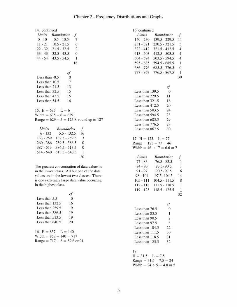
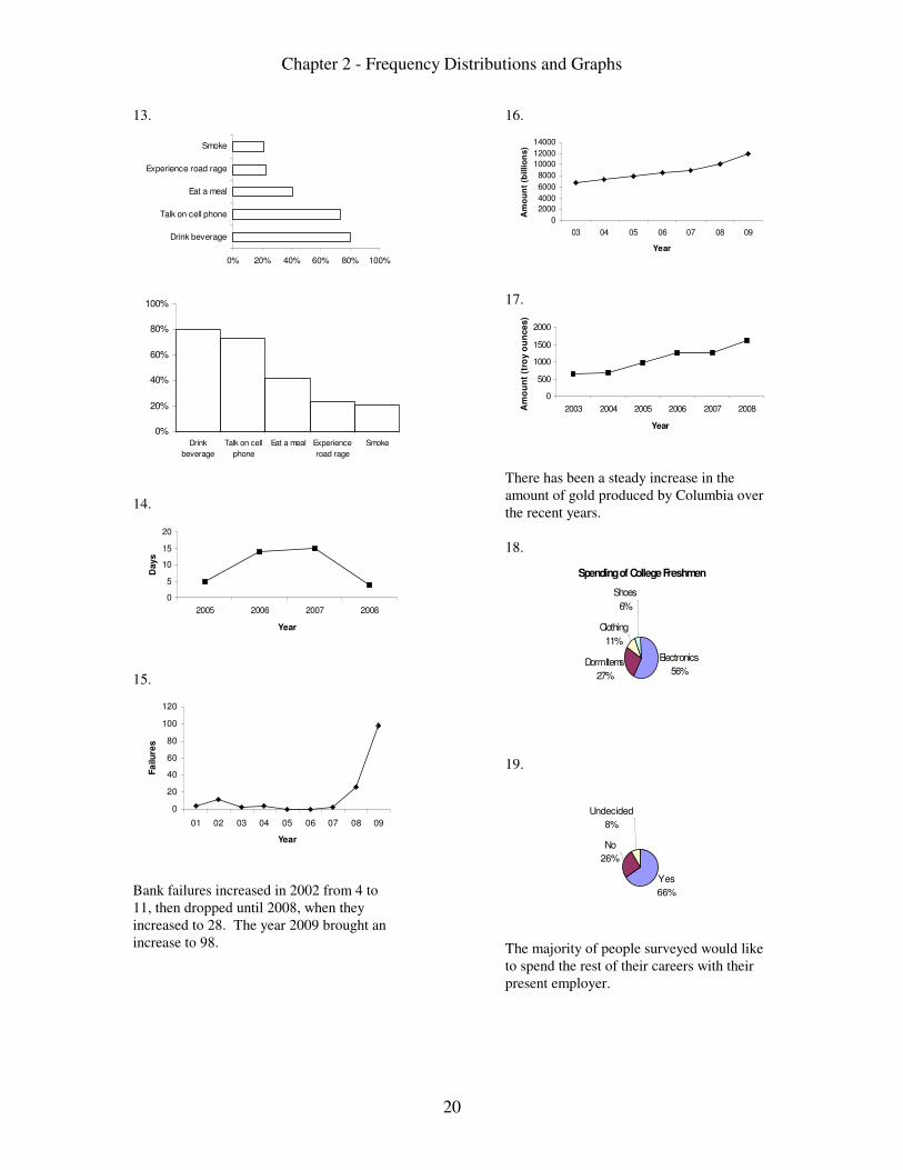
13.
0% 20% 40% 60% 80% 100%
Drink beverage
Talk on cell phone
Eat a meal
Experience road rage
Smoke
0%
20%
40%
60%
80%
100%
Drink
beverage
Talk on cell
phone
Eat a meal Experience
road rage
Smoke
14.
0
5
10
15
20
2005 2006 2007 2008
Year
Days
15.
0
20
40
60
80
100
120
01 02 03 04 05 06 07 08 09
Year
Fa
ilu
res
Bank failures increased in 2002 from 4 to11, then dropped until 2008, when theyincreased to 28. The year 2009 brought anincrease to 98.
16.
0
2000
4000
6000
8000
10000
12000
14000
03 04 05 06 07 08 09
Year
Am
ou
nt
(billio
ns)
17.
0
500
1000
1500
2000
2003 2004 2005 2006 2007 2008
Year
Am
ou
nt
(tro
y o
un
ce
s)
There has been a steady increase in theamount of gold produced by Columbia overthe recent years.
18.
Spending of College Freshmen
Electronics
56%Dorm Items
27%
Clothing
11%
Shoes
6%
19.
Yes
66%
No
26%
Undecided
8%
The majority of people surveyed would liketo spend the rest of their careers with theirpresent employer.

Chapter 2 - Frequency Distributions and Graphs
21
20.2 9 9
3 2 4 5 6 8 8
4 1 2 3 7 7
5 1 3 5 8
6 2 2 2 3 7
7 2 3
21.10 2 8 8
11 3
12
13
14 2 4
15
16
17 6 6 6
18 4 9
19 2
20 5 9
21 0
22.20 0 4 9
21 0 1 2 7 8 8
22 2 7 7 7 8
23 0 1 3 7 8
24 1 2 2 3 7
25 1 1 3 4 6
26 0
The distribution of aptitude scores is fairlyuniform.
CHAPTER 2 QUIZ
1. False2. False3. False4. True5. True6. False7. False8. c9. c10. b11. b12. Categorical, ungrouped, grouped13. 5, 2014. Categorical15. Time series16. Stem and leaf plot17. Vertical or y
18.Class f cf
H 6 6
A 5 11
M 6 17
C 25
25
8
19.
House
24%
Apartment
20%Mobile Home
24%
Condominium
32%
20.Class f
0.5 1.5 1
1.5 2.5 5
2.5 3.5 3
3.5 4.5 4
4.5 5.5 2
5.5 6.5 6
6.5 7.5 2
7.5 8.5 3
8.5 9.5
30
4
cf
less than 0.5 0
less than 1.5 1
less than 2.5 6
less than 3.5 9
less than 4.5 13
less than 5.5 15
less than 6.5 21
less than 7.5 23
less than 8.5 26
less than 9.5 30

Chapter 2 - Frequency Distributions and Graphs
22
21.
0
2
4
6
1 2 3 4 5 6 7 8 9
Items Purchased
Nu
mb
er
0
2
4
6
0 1 2 3 4 5 6 7 8 9 10
Items Purchased
Nu
mb
er
0
5
10
15
20
25
30
0.5 1.5 2.5 3.5 4.5 5.5 6.5 7.5 8.5 9.5
Items Purchased
Nu
mb
er
22.Limits Boundaries f
27 - 90 26.5 - 90.5 13
91 - 154 90.5 - 154.5 2
155 - 218 154.5 - 218.5 0
219 - 282 218.5 - 282.5 5
283 - 346 282.5 - 346.5 0
347 - 410 346.5 - 410.5 2
411 - 474 410.5 - 474.5 0
475 - 538 474.5 - 538.5 1
539 - 602 538.5 - 602.5
25
2
23.
02468
101214
26.5 -
90.5
90.5 -
154.5
154.5 -
218.5
218.5 -
282.5
282.5 -
346.5
346.5 -
410.5
410.5 -
474.5
474.5 -
538.5
538.5 -
602.5
Number of Murders
freq
ue
ncy
The distribution is positively skewed withone more than half of the data values in thelowest class.
23. continued
0
2
4
6
8
10
12
14
58.5 122.5 186.5 250.5 314.5 378.5 442.5 506.5 570.5
Number of Murders
freq
uen
cy
0
5
10
15
20
25
30
26.5 90.5 154.5 218.5 282.5 346.5 410.5 474.5 538.5 602.5
Number of Murders
cu
mu
lati
ve f
req
uen
cy
24.
0
100
200
300
400
Paper Iron/Steel Aluminum Yard
waste
Glass Plastics
To
ns
0 100 200 300 400
Paper
Iron/steel
Aluminum
Yard Waste
Glass
Plastics
Typ
e o
f W
as
te
Tons

Chapter 2 - Frequency Distributions and Graphs
23
25.
Identity Thefts
Lost or
stolen item
45%
Retail
purchases
18%
Stolen mail
11%
Computer
checks
9%
Phishing
5%
Other
12%
26.
0
1000
2000
3000
4000
2020 2025 2030 2035
Year
Nu
mb
er
of
dea
ths
27.1 5 9
2 6 8
3 1 5 8 8 9
4 1 7 8
5 3 3 4
6 2 3 7 8
7 6 9
8 6 8 9
9 8
Elementary Statistics A Step by Step Approach 8th Edition Bluman Solutions ManualFull Download: http://alibabadownload.com/product/elementary-statistics-a-step-by-step-approach-8th-edition-bluman-solutions-manual/
This sample only, Download all chapters at: alibabadownload.com
Top Related