Wireframe-Free Geological Modelling – An Oxymoron … · Mine operations demand accurate 3D...

EIGHTH INTERNATIONAL MINING GEOLOGY CONFERENCE / QUEENSTOWN, NEW ZEALAND, 22 - 24 AUGUST 2011 1

INTRODUCTIONMine operations demand accurate 3D geological models for estimating resources. The industry-wide accepted method for constructing such models is to use wireframes to outline the ore-waste boundary. However, this method is costly; it may take days or weeks to produce the 3D wireframes by sectional digitisation, the subsequent time-consuming 3D tying process and wireframe validation. The mining industry would benefit from faster modelling methods that circumvent this time-

consuming process. A discussion of an alternative modelling method is the subject of this research paper.

Implicit modelling methods deliver accurate models rapidly, without needing time-consuming sectional digitisation (Cowan et al, 2003). Implicit models allow the export of results direct to a block model, without needing to construct detailed wireframes. Skipping this time-consuming workflow could improve the long-term profitability of mining operations,

1. Director, Prestologic Pty Ltd, PO Box 230, Fremantle WA 6959. Email: [email protected]

2. Research Engineer, ARANZ Geo Ltd, PO Box 3894, Christchurch 8140, New Zealand. Email: [email protected]

3. MAusIMM, Geology Manager, Grange Resources Ltd, Level 11, 200 St Georges Terrace, Perth WA 6000. Email: [email protected]

Wireframe-Free Geological Modelling – An Oxymoron or a Value Proposition?E J Cowan1, K J Spragg2 and M R Everitt3

ABSTRACTEfficiency demands that mine geologists devote the most time to tasks where they can have the biggest effect on production. One of the most time-consuming tasks is geological interpretation of the orebody and turning this into a block model for the planning engineers.

The current best practice for mines that require a geologically constrained resource model involves capturing the interpretation of geologists as three-dimensional (3D) wireframes. However, there is significant overhead in the production of valid wireframes from sectional and plan interpretations. This overhead consists of the mundane tasks of digitising polylines, then building 3D wireframes and validating them. While software can simplify this task, the current process is not the best use of a geologist’s time. Under time pressure exerted by planning engineers and the time required for modelling from polylines, geologists are forced to roll-up the presence of other elements or impurities into the interpretation and encode them in the polylines, even though it is often desirable to consider these other factors separately.

While it might seem unlikely that mine geologists can produce constrained geological models without the intermediary of wireframes, the technology to accomplish this is getting closer.

In this paper, the results of a trial at the Savage River magnetite mine, which is owned and operated by Grange Resources Ltd, are reported. The trial was for a ‘direct-to-block’ implicit geological modelling method. The focus was on creating a geological attributed block model from drill hole geological log data; resource estimates were not determined. The categories modelled were air, waste, low-grade ore, medium-grade ore, and high-grade ore. The block model outputs either resulted in a proportional block model (categories expressed as percentages within equivolumetric blocks) or a sub-blocked model (parent block and one sub-block), which is the preferred block model output at the Savage River mine. When compared to the traditional best practice modelling method, which takes 43 work days, the wireframe-free modelling method took only 26 hours from initial modelling, using both exploration and grade control data. An update using appended drill hole data is achievable within one day. These results represent time savings of more than one order of magnitude compared to the traditional workflow, and, as such, these figures merit serious consideration for the use of the direct-to-block modelling approach at other operations.

With these time savings, geological and estimation models can be kept updated constantly; geologists will not need to set aside two months for quarterly or half-yearly modelling of the drill hole data for resource review. Such dramatic time savings will allow for the better use of highly skilled geologists, who are in short supply in the current market, and will also impact directly on downstream mining engineering workflows.

Cowan.indd 1 6/07/2011 3:45:39 PM

EIGHTH INTERNATIONAL MINING GEOLOGY CONFERENCE / QUEENSTOWN, NEW ZEALAND, 22 - 24 AUGUST 2011

E J COWAN, K J SPRAGG AND M R EVERITT

2

and allow the assessment of risks associated with geological interpretations in a way not possible before.

This implicit modelling method was tested on drill hole data from Savage River magnetite mine in north-west Tasmania, operated by Grange Resources Ltd. Our approach for defining the ore-waste boundary, as well as three internal ore zones (low-, medium- and high-grade), demonstrated the effectiveness of the method, as it compressed the workflow from 43 days to just two days or fewer. Refreshing the model with additional drill hole data would further reduce the time taken.

Before discussing methods and implications, background is provided as to why the traditionally accepted modelling method is so dependent on validated wireframes.

ARE WIREFRAMES ESSENTIAl FOR GEOlOGICAl MODEllING?Wireframes are generally regarded as essential to the geological modelling process. Whilst this is true for hand-digitised wireframe modelling methods, it is not a requirement for implicit modelling (Figure 1). The two modelling methods are outlined and compared below.

Explicit modelling workflowThe construction of wireframes in geological modelling is a modification of drawing methods used in the vector-based computer-aided design (CAD) software products initially developed for the field of industrial design. At a basic level, the user of two-dimensional CAD software can draw sectional lines to construct object outlines (strings or polylines). The 3D wireframing process is simply an extension of this 2D drawing process, where all lines are manually joined by adding tie

lines that link nodes from one sectional polyline to another. Because the geologist must explicitly digitise each and every node, this modelling process is termed ‘explicit modelling’.

Sectional polylines that are tied in three dimensions are an ambiguous representation of a solid volume. The object is literally a ‘wireframe’ – it does not contain embedded information regarding the positions that are inside or outside the object. Without this critical information concerning the object interface positions in space, the wireframe cannot be used immediately for two essential tasks that are required for resource modelling:

1. selecting assay data in space (usually expressed as mid-points of assay composite intervals); and

2. documenting the interpreted shape and volume of the orebody in 3D, which informs the percentage of ore/lithology within a particular block in a block model.

For computer software to determine the inside and outside of this object, the tied polylines must be converted into a triangulation surface model. That is, the surface at any position defined by a triangulation face then becomes a part of a continuous surface of a solid object. For the above two tasks to be completed, it is essential that the wireframe model is closed, and that the triangulation facets (which have facing directions) are all consistently orientated.

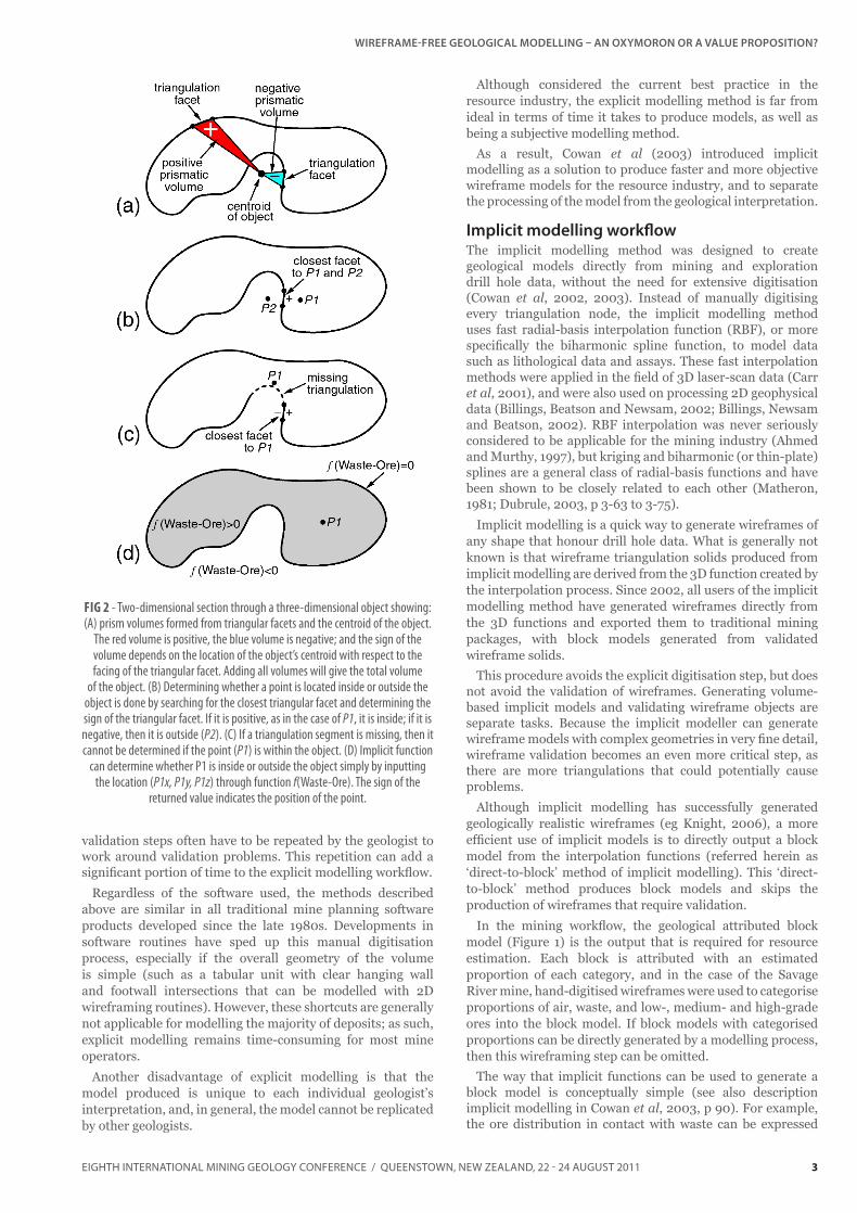
To better understand why imperfections of triangulation models must be eliminated, one of the methods of volume computation is outlined in Figure 2a. By convention, triangulation facets have a positive and negative side. Once all positive faces of the triangulations are facing consistently inward to the closed object, the centroid of the closed object is determined. Prismatic volumes are then computed between each triangulation facet and the centroid of the object. If the object is curved like a banana, with the centroid lying outside the object, the object’s volume can still be determined by using the sign of the triangular faces (Figure 2a). If the centroid is lying on the positive side of the triangular facet, this will generate a positive volume. If the centroid is on the negative side, the volume will be negative. The object’s total volume is the sum of all prismatic volumes generated by all the triangular facets with the centroid of the object.

If triangulations are missing, or the sign of triangulation facets are not consistently orientated, the resulting volume will be inaccurate. Most geological modelling software programs will not allow volumes to be computed unless the object is closed.

The selection of points within an object also requires a closed object with consistently facing triangulations (Figure 2b). To select points within an object, the closest triangulation is determined for each point, and, if the point is located on the positive side of the closest triangulation facet, it is considered to be within the object. If the triangulation facet is locally reversed, or if it is missing (Figure 2c), the software program cannot accurately select the points within the modelled object. For example, self-intersecting triangulations where the positive face of triangulations face outwards, will result in points being selected outside the object.

Although there are several methods for volume calculations and point selections, no method can achieve the tasks listed above without closed triangulation objects that have consistently orientated faces. In the polyline tying process, it is common for the solid to develop invalid triangulation facets that might intersect each other. Because these imperfections must be eliminated before an accurate volume of the object can be calculated, the tying process and triangulation

Fig 1 - (A) Comparison between the traditional explicit modelling workflow; and (B) the direct-to-block implicit modelling workflow. Greyed areas are time-consuming parts of the explicit modelling workflow. Note that the triangulation in the implicit workflow is only used for a visual check of the modelling and the

wireframes are not used for the construction of the block model.

Cowan.indd 2 6/07/2011 3:45:40 PM


WIREFRAME-FREE GEOlOGICAl MODEllING – AN OxyMORON OR A VAlUE PROPOSITION?

3

validation steps often have to be repeated by the geologist to work around validation problems. This repetition can add a significant portion of time to the explicit modelling workflow.

Regardless of the software used, the methods described above are similar in all traditional mine planning software products developed since the late 1980s. Developments in software routines have sped up this manual digitisation process, especially if the overall geometry of the volume is simple (such as a tabular unit with clear hanging wall and footwall intersections that can be modelled with 2D wireframing routines). However, these shortcuts are generally not applicable for modelling the majority of deposits; as such, explicit modelling remains time-consuming for most mine operators.

Another disadvantage of explicit modelling is that the model produced is unique to each individual geologist’s interpretation, and, in general, the model cannot be replicated by other geologists.

Although considered the current best practice in the resource industry, the explicit modelling method is far from ideal in terms of time it takes to produce models, as well as being a subjective modelling method.

As a result, Cowan et al (2003) introduced implicit modelling as a solution to produce faster and more objective wireframe models for the resource industry, and to separate the processing of the model from the geological interpretation.

Implicit modelling workflowThe implicit modelling method was designed to create geological models directly from mining and exploration drill hole data, without the need for extensive digitisation (Cowan et al, 2002, 2003). Instead of manually digitising every triangulation node, the implicit modelling method uses fast radial-basis interpolation function (RBF), or more specifically the biharmonic spline function, to model data such as lithological data and assays. These fast interpolation methods were applied in the field of 3D laser-scan data (Carr et al, 2001), and were also used on processing 2D geophysical data (Billings, Beatson and Newsam, 2002; Billings, Newsam and Beatson, 2002). RBF interpolation was never seriously considered to be applicable for the mining industry (Ahmed and Murthy, 1997), but kriging and biharmonic (or thin-plate) splines are a general class of radial-basis functions and have been shown to be closely related to each other (Matheron, 1981; Dubrule, 2003, p 3-63 to 3-75).

Implicit modelling is a quick way to generate wireframes of any shape that honour drill hole data. What is generally not known is that wireframe triangulation solids produced from implicit modelling are derived from the 3D function created by the interpolation process. Since 2002, all users of the implicit modelling method have generated wireframes directly from the 3D functions and exported them to traditional mining packages, with block models generated from validated wireframe solids.

This procedure avoids the explicit digitisation step, but does not avoid the validation of wireframes. Generating volume-based implicit models and validating wireframe objects are separate tasks. Because the implicit modeller can generate wireframe models with complex geometries in very fine detail, wireframe validation becomes an even more critical step, as there are more triangulations that could potentially cause problems.

Although implicit modelling has successfully generated geologically realistic wireframes (eg Knight, 2006), a more efficient use of implicit models is to directly output a block model from the interpolation functions (referred herein as ‘direct-to-block’ method of implicit modelling). This ‘direct-to-block’ method produces block models and skips the production of wireframes that require validation.

In the mining workflow, the geological attributed block model (Figure 1) is the output that is required for resource estimation. Each block is attributed with an estimated proportion of each category, and in the case of the Savage River mine, hand-digitised wireframes were used to categorise proportions of air, waste, and low-, medium- and high-grade ores into the block model. If block models with categorised proportions can be directly generated by a modelling process, then this wireframing step can be omitted.

The way that implicit functions can be used to generate a block model is conceptually simple (see also description implicit modelling in Cowan et al, 2003, p 90). For example, the ore distribution in contact with waste can be expressed

Fig 2 - Two-dimensional section through a three-dimensional object showing: (A) prism volumes formed from triangular facets and the centroid of the object.

The red volume is positive, the blue volume is negative; and the sign of the volume depends on the location of the object’s centroid with respect to the facing of the triangular facet. Adding all volumes will give the total volume

of the object. (B) Determining whether a point is located inside or outside the object is done by searching for the closest triangular facet and determining the sign of the triangular facet. If it is positive, as in the case of P1, it is inside; if it is negative, then it is outside (P2). (C) If a triangulation segment is missing, then it cannot be determined if the point (P1) is within the object. (D) Implicit function

can determine whether P1 is inside or outside the object simply by inputting the location (P1x, P1y, P1z) through function f(Waste-Ore). The sign of the

returned value indicates the position of the point.

Cowan.indd 3 6/07/2011 3:45:40 PM



4

as a 3D function that is saved on the computer (Figure 2d). To determine whether a point (P1) is located inside or outside the ore, the point position (P1x, P1y, P1z) is entered into the function f(Waste-Ore). If the returned value is positive (f(Waste-Ore)>0), then P1 is within the ore (Figure 2d); if f(Waste-Ore) <0, then it is outside; and if f(Waste-Ore) = 0, then P1 is located on the boundary between waste and ore. This method does not require any knowledge of the nearest triangulation facet to P1, so it is easy to understand and will work on any complex 3D geometry. To export the categorised data to a block model, this process is repeated with a 3D grid for all categories modelled. The proportion of each category can then be determined for each block, without requiring validated wireframes to generate the block model.

The primary benefit of this modelling method is the reduction of time. As shown in the case study, using the traditional workflow to generate the block model took more than 40 days; the implicit modelling method reduced this to two days or fewer. This represents more than one order of magnitude in time saving.

The direct-to-block modelling method was trialled at the Savage River magnetite deposit; the details and initial results are discussed below.

CASE STUDy – SAVAGE RIVER MAGNETITE DEPOSITThe Savage River magnetite mine in north-west Tasmania (Figure 3) has operated for more than 40 years. It is an open cut mine, which has produced a concentrate of approximately 67 per cent Fe by means of magnetic separation at a rate varying between 1.4 and 2.4 Mt/a. The mining operation was undertaken by Australian Bulk Minerals from 1997 until December 2008, when Australian Bulk Minerals merged with Grange Resources Ltd.

In 2008, when the case study was undertaken, the operation had an expected mine life of about 15 years, based on the expansion of North Pit. Other resources on the mine lease could potentially extend this mine life out to about 25 years. The total resource, including inferred material, as at 31 March 2008 was 323 Mt at a grade of 51 per cent Davis Tube Recovery (DTR), with a reserve of 131 Mt at 49 per cent DTR.

The Savage River magnetite deposits occur in a belt of greenschist facies metamorphics of Cambrian age, known as the Arthur Metamorphic Complex. The metamorphic complex is up to 10 km wide and runs NNE across north-western Tasmania for some 110 km from the west coast to the north coast (Figure 3). It corresponds with a tectonic feature known as the Arthur Lineament and forms a boundary zone between relatively unmetamorphosed, Proterozoic shelf deposits to the west and relatively unmetamorphosed, Proterozoic turbidite deposits to the east.

The Bowry Creek Formation of the Arthur Metamorphics contains the Savage River magnetite deposits as well as a semi-continuous line of smaller magnetite deposits to the south of the mine lease. Altogether, the magnetite deposits reflect an iron formation with a strike length of about 30 km.

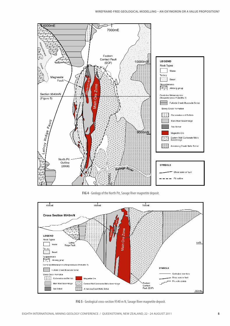
The magnetite ore is bounded on the eastern side by a fault known as the ECF. The spatial position of ECF is defined by the ore termination and is also defined by the presence of the unmineralised Armstrong Creek Mafic Schist (drill hole lithocode MXR), a submember of the Bowry Creek Formation, to the east. The magnetite ore is sharply truncated by this subvertical fault and is only present on the western side of ECF (Figures 4 and 5).

The data used for this study were resource drilling and grade control data from the North Pit (north of 8000 m N; see Figure 4) that were available prior to March 2007. The results of the modelling undertaken for the resource estimation (Model NP307) and the implicit modelling results are compared.

Fig 3 - Geological setting and location of the Savage River magnetite deposit in north-west Tasmania.

Cowan.indd 4 6/07/2011 3:45:41 PM



5

Fig 4 - Geology of the North Pit, Savage River magnetite deposit.

Fig 5 - Geological cross-section 9540 m N, Savage River magnetite deposit.

Cowan.indd 5 6/07/2011 3:45:42 PM



6

SAVAGE RIVER MINE ExPlICIT MODEllING WORKFlOWThe following sections describe the traditional explicit modelling procedure used at the Savage River mine.

Geological interpretationBlock models were built and maintained for each individual Pit. Prior to a block model update, geological interpretations were compiled and updated. The process commenced with the acquisition of pit mapping data, drill hole data, and grade control data, followed by an interpretation on cross-section, which was then refined on flitch plans.

Assay methodsFor the Savage River magnetite deposits, the ore grade was expressed as the percentage of material in the ore that could be recovered in a Davis Tube, under standard conditions. This percentage is known as the Davis Tube Recovery or DTR. The Davis Tube simulated the recovery of magnetite in the Savage River concentrator. Routine assays for total iron, nickel (Ni), titanium (TiO

2), magnesium (MgO), phosphorus

(P), vanadium (V), sulfur (S), and silicon (SiO2) were carried

out by XRF methods.

Sectional interpretationCross-sections through the entire deposit at 50 m spacing were generated and plotted on to A1 paper. Each section comprised drill holes with lithology codes, DTR grades, the natural surface topography, and various pit surfaces that correlated with successive mapping campaigns. The latest interpretation for North Pit included plots of grade control sample data that illustrated the historical distribution of grade, and assisted in projecting boundaries between drill holes.

Each section was interpreted for magnetite mineralisation and waste rock types. Histogram plots of DTR displayed a bimodal distribution of the mineralisation with a third, more subtle, population in the medium-grade ranges. These populations defined the boundaries of the lithological subdivision of the mineralisation in drill logging and mapping, ie abundant (DTR >65 per cent), moderate (35 - 65 per cent DTR), and sparse (15 - 35 per cent DTR) categories. The relationship between abundant and moderate mineralisation is often too complex to be modelled sectionally, and these two categories are usually combined to form one outline for high-grade ore (ie DTR >35 per cent), with another outline for low-grade ore (15 per cent <DTR <35 per cent).

Waste rocks were assigned a rock type code that indicated their potential for acid generation used to assist in environmental management and scheduling purposes. Interpretations on each section were digitised using a traditional mine planning software program, with each mineralisation or waste rock boundary assigned a predefined polyline number. Boundaries were manually snapped to drill hole contacts, where appropriate.

Flitch InterpretationThe corrected section files were sliced horizontally at 10 m intervals throughout the vertical extent of the model to produce a series of coded cut bar files that were used to form the basis of the flitch interpretation. Flitch plans, comprising drill hole data and cut bars, were plotted for every 10 m interval.

Each flitch was interpreted for magnetite mineralisation and subdivided into ‘abundant-moderate’ and ‘sparse’ magnetite

categories. Waste rocks were assigned a rock type code that indicated their potential for acid generation.

Individual flitch shapes were digitised, edited and corrected into 10 m spaced flitch ore files to form the basis of the mineralisation wireframe.

Wireframe constructionWireframes were constructed from the 10 m flitch outlines for abundant-moderate and sparse magnetite mineralisation, and waste rock types. Due to the complexity of the relationships between high-grade, low-grade and internal waste zones, the wireframes were constructed with a fixed sequence of overprinting in mind. High-grade ore shapes were constructed first. These may be overprinted by low-grade ore shapes, and both may be overprinted by internal waste zones. Although this meant that the ore shapes could not be viewed in isolation, it did significantly reduce the time required to model the multitude of tiny shapes required to make each material a standalone set of wireframes.

The resultant wireframe shapes were validated and set to solids.

Time frame requirements for the explicit modelling workflowThe modelling process outlined above, excluding resource estimation, took over a month to complete. Due to the time required, other impurities or elements were not modelled individually, although the abundance of V and TiO

2 were

monitored to keep the product within required specifications. Due to the time-consuming process, model updates were only undertaken when there was significant new information available. The time taken for each modelling step is summarised in Table 1.

SAVAGE RIVER MINE DIRECT-TO-BlOCK IMPlICIT MODEllING WORKFlOWThe direct-to-block implicit modelling of individual geological categories from the Savage River exploration drilling and grade control data was completed in two steps:

1. implicit modelling of each category (air, waste, low-grade ore, medium-grade ore, and high-grade ore); and

2. direct-to-block block model export of the implicit geological model.

Task Days (hours)Data collation and plotting 40 cross-sections 2 (16)

Sectional interpretation 10 (80)

Sectional digitising 5 (40)

Slicing and plotting 110 flitch plans 1 (8)

Flitch interpretation 5 (40)

Flitch digitising 5 (40)

Wireframe modelling and validation 15 (120)

Total 43 days (344 hours)

Table 1

Explicit modelling workflow at Savage River magnetite mine. Time estimates are based on a five-day, eight-hour/day working week for one person working continuously, although different people may contribute in parallel to different

stages of the modelling.

Cowan.indd 6 6/07/2011 3:45:42 PM



7

This modelling exercise replicated the outputs of the traditional workflow, using identical input categories as defined by Grange Resources Ltd.

Implicit modelling of multiple categorical dataFor a background of how categorical data can be modelled implicitly, refer to Cowan et al (2003).

Categorical data cannot be interpolated unless they are converted to numerical point values (expressed as x, y, z, numerical value). Once converted, these 3D point values are interpolated with a radial basis function with a zero nugget linear variogram to ensure an exact honouring of the categorical boundaries. A linear variogram ensures that the contact between lithologies may exist between widely spaced exploration drill holes.

The conversion of categorical data to numerical data is conducted in reference to a boundary defined by two categories that are in contact with each other (Cowan et al, 2003; Figures 1c - 1d). For example, the ECF is a surface that cuts the ore, east of which is waste, so this boundary position must be accurately modelled. However, this boundary shape is not explicitly digitised, as required by the explicit modelling workflow; instead, the observed ECF intersection points in the drill hole data, as well as the ECF trace points along the erosion surface, are given a numerical value of zero. Points along the drill holes that are located on the western side can be assigned positive distance values away from the fault, and points on the eastern side can be assigned negative distance values from the ECF. Once these sets of points, which have a gradient from negative to positive values, are interpolated, the f(ECF) = 0 value defines the ECF position in space. The eastern side of the ECF is defined as f(ECF) >0 and the western side as f(ECF) <0. To determine where any point is located in space relative to the ECF, the point’s position (x, y, z) is input into f(ECF); the output value indicates where the point is located relative to the ECF.

The volume function representing the spatial position of two adjacent geological categories (eg ore versus waste) is modelled separately from the other paired categorical boundaries (Figures 6a - 6e). There are advantages to this simple modelling method. For example, a particular categorical boundary is likely to have its own unique continuity orientation, which can be represented by a smooth interpolation function. This is not only logical but is a practical necessity from the perspective of numerical interpolation. For example, the Savage River topography has a subhorizontal orientation, whereas the ECF is vertical, and the ore-waste boundary has a completely different orientation to these contacts. It is impossible to model all these boundary features using a single interpolation function because the boundaries between these are sharp ,whereas interpolation functions are smooth and lack discontinuities.

By contrast, if the volumes are modelled as separate volume functions and later combined by taking into consideration geological superposition, the resulting 3D model will be realistic geologically and it can contain sharp junctures (Figure 6f). Since continuities of these individual volume functions defined by paired categories are all different, it is simple to define each one separately, thus making it a very practical approach for modelling. Geological models consisting of multiple lithologies, with complex but geologically reasonable interlocking relationships, can be modelled easily once the geological chronology is established.

The above method of modelling multiple categorical data contrasts with the explicit modelling method, where multiple

boundary types are represented along an explicitly digitised sectional polyline loop. For example, a polyline that represents the medium-grade ore boundary (as shown in Figure 6f) may contain polyline segments that represent the medium-grade ore in contact with the low-grade ore, as well as the contact with ECF, topography, and the high-grade ore.

Closed polyline loops are therefore composite boundary polylines, with each segment having its own unique spatial continuity in space; because of this composite character, it is impractical to model this type of data numerically. The difficulties faced during the tying of polyline loops from section to section is partly a result of the composite characteristics of the closed digitised loops. In addition, explicit methods must deal with multiple merging and splitting of objects from section to section. The yellow medium-grade outlines shown in Figure 6f are split into two in this section, but may coalesce in another section. This splitting and joining is a complex and time-consuming part of explicit modelling workflow. This complexity does not exist in implicit modelling because of the use of superposed volume functions (Figure 6).

Savage River categorical implicit functionsFive functions were established to model the various categories required for the Savage River block model. Once modelled, the shape of each contact surface was checked by visually examining (on screen) the isosurface representation (triangulations) of each boundary. These isosurfaces were

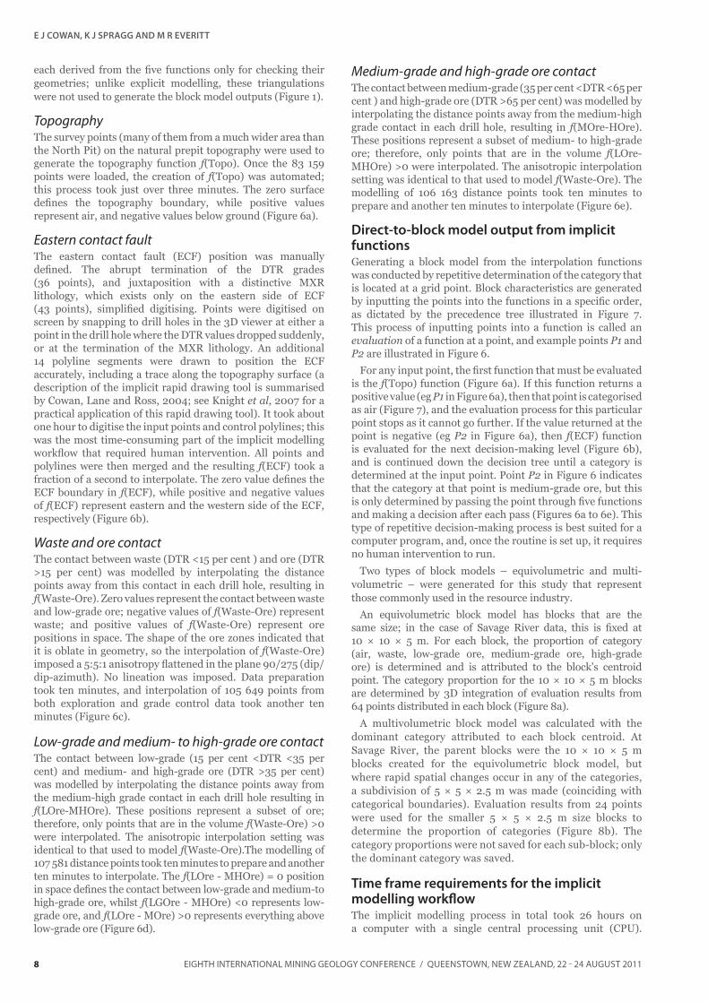
Fig 6 - (A - E) Multiple implicit functions representing five different contact relationships at the Savage River deposit. An idealised section viewing north

(similar to Figure 5). The positive areas of the functions are shown in grey; white shows the negative areas. The functions are placed in order of precedence relating to geology. (F) shows the final model taking overlapping relationships into account. L = low-grade ore; M = medium-grade ore; H = high-grade ore.

Points P1 and P2 are discussed in text.

Cowan.indd 7 6/07/2011 3:45:43 PM



8

each derived from the five functions only for checking their geometries; unlike explicit modelling, these triangulations were not used to generate the block model outputs (Figure 1).

TopographyThe survey points (many of them from a much wider area than the North Pit) on the natural prepit topography were used to generate the topography function f(Topo). Once the 83 159 points were loaded, the creation of f(Topo) was automated; this process took just over three minutes. The zero surface defines the topography boundary, while positive values represent air, and negative values below ground (Figure 6a).

Eastern contact faultThe eastern contact fault (ECF) position was manually defined. The abrupt termination of the DTR grades (36 points), and juxtaposition with a distinctive MXR lithology, which exists only on the eastern side of ECF (43 points), simplified digitising. Points were digitised on screen by snapping to drill holes in the 3D viewer at either a point in the drill hole where the DTR values dropped suddenly, or at the termination of the MXR lithology. An additional 14 polyline segments were drawn to position the ECF accurately, including a trace along the topography surface (a description of the implicit rapid drawing tool is summarised by Cowan, Lane and Ross, 2004; see Knight et al, 2007 for a practical application of this rapid drawing tool). It took about one hour to digitise the input points and control polylines; this was the most time-consuming part of the implicit modelling workflow that required human intervention. All points and polylines were then merged and the resulting f(ECF) took a fraction of a second to interpolate. The zero value defines the ECF boundary in f(ECF), while positive and negative values of f(ECF) represent eastern and the western side of the ECF, respectively (Figure 6b).

Waste and ore contactThe contact between waste (DTR <15 per cent ) and ore (DTR >15 per cent) was modelled by interpolating the distance points away from this contact in each drill hole, resulting in f(Waste-Ore). Zero values represent the contact between waste and low-grade ore; negative values of f(Waste-Ore) represent waste; and positive values of f(Waste-Ore) represent ore positions in space. The shape of the ore zones indicated that it is oblate in geometry, so the interpolation of f(Waste-Ore) imposed a 5:5:1 anisotropy flattened in the plane 90/275 (dip/dip-azimuth). No lineation was imposed. Data preparation took ten minutes, and interpolation of 105 649 points from both exploration and grade control data took another ten minutes (Figure 6c).

Low-grade and medium- to high-grade ore contactThe contact between low-grade (15 per cent <DTR <35 per cent) and medium- and high-grade ore (DTR >35 per cent) was modelled by interpolating the distance points away from the medium-high grade contact in each drill hole resulting in f(LOre-MHOre). These positions represent a subset of ore; therefore, only points that are in the volume f(Waste-Ore) >0 were interpolated. The anisotropic interpolation setting was identical to that used to model f(Waste-Ore).The modelling of 107 581 distance points took ten minutes to prepare and another ten minutes to interpolate. The f(LOre - MHOre) = 0 position in space defines the contact between low-grade and medium-to high-grade ore, whilst f(LGOre - MHOre) <0 represents low-grade ore, and f(LOre - MOre) >0 represents everything above low-grade ore (Figure 6d).

Medium-grade and high-grade ore contactThe contact between medium-grade (35 per cent <DTR <65 per cent ) and high-grade ore (DTR >65 per cent) was modelled by interpolating the distance points away from the medium-high grade contact in each drill hole, resulting in f(MOre-HOre). These positions represent a subset of medium- to high-grade ore; therefore, only points that are in the volume f(LOre-MHOre) >0 were interpolated. The anisotropic interpolation setting was identical to that used to model f(Waste-Ore). The modelling of 106 163 distance points took ten minutes to prepare and another ten minutes to interpolate (Figure 6e).

Direct-to-block model output from implicit functionsGenerating a block model from the interpolation functions was conducted by repetitive determination of the category that is located at a grid point. Block characteristics are generated by inputting the points into the functions in a specific order, as dictated by the precedence tree illustrated in Figure 7. This process of inputting points into a function is called an evaluation of a function at a point, and example points P1 and P2 are illustrated in Figure 6.

For any input point, the first function that must be evaluated is the f(Topo) function (Figure 6a). If this function returns a positive value (eg P1 in Figure 6a), then that point is categorised as air (Figure 7), and the evaluation process for this particular point stops as it cannot go further. If the value returned at the point is negative (eg P2 in Figure 6a), then f(ECF) function is evaluated for the next decision-making level (Figure 6b), and is continued down the decision tree until a category is determined at the input point. Point P2 in Figure 6 indicates that the category at that point is medium-grade ore, but this is only determined by passing the point through five functions and making a decision after each pass (Figures 6a to 6e). This type of repetitive decision-making process is best suited for a computer program, and, once the routine is set up, it requires no human intervention to run.

Two types of block models – equivolumetric and multi-volumetric – were generated for this study that represent those commonly used in the resource industry.

An equivolumetric block model has blocks that are the same size; in the case of Savage River data, this is fixed at 10 × 10 × 5 m. For each block, the proportion of category (air, waste, low-grade ore, medium-grade ore, high-grade ore) is determined and is attributed to the block’s centroid point. The category proportion for the 10 × 10 × 5 m blocks are determined by 3D integration of evaluation results from 64 points distributed in each block (Figure 8a).

A multivolumetric block model was calculated with the dominant category attributed to each block centroid. At Savage River, the parent blocks were the 10 × 10 × 5 m blocks created for the equivolumetric block model, but where rapid spatial changes occur in any of the categories, a subdivision of 5 × 5 × 2.5 m was made (coinciding with categorical boundaries). Evaluation results from 24 points were used for the smaller 5 × 5 × 2.5 m size blocks to determine the proportion of categories (Figure 8b). The category proportions were not saved for each sub-block; only the dominant category was saved.

Time frame requirements for the implicit modelling workflowThe implicit modelling process in total took 26 hours on a computer with a single central processing unit (CPU).

Cowan.indd 8 6/07/2011 3:45:43 PM



9

Fig 7 - An input point must be passed through the functions in this order of precedence to determine the category at any point (air, waste, or three of the ore grade categories). Obtaining a block model repeats this process at grid points to determine the proportion of each category within a block.

Fig 8 - Evaluation points weighting scheme for 3D integration to compute the proportion of categories within (A) 10 × 10 × 5 m blocks, and (B) 5 × 5 × 2.5 m blocks.

Cowan.indd 9 6/07/2011 3:45:44 PM



10

The most time-consuming step is the creation of the block outputs, but this workflow can be shortened using a multi-core processor (Table 2). Updating the model with extra drill hole information requires only the new drill holes to be appended into the project and then reprocessed. If there are no major changes to the geological interpretation, a new block model can be regenerated within a day of the new data being imported. The direct-to-block implicit modelling method compressed what took more than 40 days to complete down to two days.

Comparison between block model resultsComparison of the direct-to-block results with the NP307 block model outputs were complicated because the NP307 model consisted of six block sizes, whereas the sub-blocked model had only two sizes. To obtain a fair comparison between the two methods the block centroids of both models were selected within a distance of 60 m away from the drill hole samples that were used to create the models. The waste

and ore category volumes are summarised in Table 3. The low waste volume in the NP307 model is likely due to missing large block centroids at the edges of the distance-based selection envelope. The total volume of ore is similar between the explicit and implicit models; only the internal allocation of low-grade to high-grade is different.

Blocks plotted in sections compared favourably (Figures 9 and 10). There appears to be more ore allocated in the explicit model, especially at depth. This may be due to the assumption that the orebody continuity is vertical, when it is most likely plunging to the south, which would explain some tapering at depth in the implicit model.

The models were also compared in a smaller selected volume, well away from large peripheral blocks of the NP307 model (Table 4). The total volume is closer as there are fewer larger blocks in the NP307 model. Again, the results of the implicit block models are very similar to that produced by explicit modelling, although more detail can be discerned from visual comparisons (Figure 11). The advantage of the direct-to-block method is that it allows the separation of the medium-grade ore from the high-grade ore. This separation was never achieved with explicit modelling due to the time it would take to differentiate these two categories by hand digitisation.

CONClUSIONSThe research conducted with the Savage River data shows that validated wireframes are not necessary for the production of high-quality block models for resource estimation. The advantages of the direct-to-block modelling method using implicit functions are many, including:

• Substantially reduced modelling time: at the Savage River mine, the direct-to-block modelling method took 26 hours to produce a block model, compared to 43 days using digitising (Tables 1 and 2). The implicit modelling method will lead to more efficient time usage by the mine geologists, who are in short supply in the current market. The reduced modelling time merits serious consideration for the direct-to-block modelling approach at other mining operations.

• Faster block model updates: at Savage River, models are updated with newly acquired drill hole data simply by loading the new data. The update process to generate a new block model will only take one work day. Effectively, block models can be updated weekly, rather than setting aside two months for half-yearly or annual modelling of the drill hole data for resource review.

• Superior accuracy: the accuracy of the implicit model output is far superior to hand-digitised outputs. Much of the grade control data was not modelled with hand

Category NP307 block model volume (% of total)

Direct-to-block equivolumetric (10 × 10 × 5 m) block model

volume (% of total)

Direct-to-block multivolumetric (10 × 10 × 5 m, 5 × 5 × 2.5 m)

block model volume (% of total)Waste 113.4 (63.4%) 136.6 (71.0%) 138.2 (71.8%)

Low-grade ore 12.2 (7.2%) 17.2 (8.9%) 16.2 (8.4%)

Medium-grade ore Not differentiated with high-grade ore 21.6 (11.2%) 20.6 (10.7%)

High-grade ore 42.8 (25.4%) 16.9 (8.8%) 17.4 (9.0%)

Total volume (× 106 m3) 168.4 of which 55.0 is ore 192.3 of which 55.7 is ore 192.3 of which 54.2 is ore

Table 3

Volumetric comparison of the block models for the entire study area. Volumes are expressed in million m3. The high-grade ore in the NP307 model is a combination of medium- and high-grade ore.

Task Minutes (hours)Setting up project and import data 60 (1)

Defining the topography function f(Topo) 3 (0.05)

Defining the ECF function f(ECF) 60 (1)

Defining the waste-ore contact function f(Waste-Ore)

20 (0.33)

Defining the low-grade to medium and high-grade contact function f(LOre-MHOre)

20 (0.33)

Defining the medium-grade to high-grade contact function f(MOre-HOre)

20 (0.33)

Percentage proportional equivolumetric block model (10 × 10 × 5 m)

660 (11)/165(2.75)*

Subdivided block model (10 × 10 × 5 m and 5 × 5 × 2.5 m)

720 (12)/180 (3)*

Total1563 minutes (26 hours) for single core CPU 528 minutes

(8.8 hours) for a quad-core CPU

* The last two tasks generating the block models require no human intervention and represent computational time only. The computation tasks were performed on a single core central processing unit (CPU), but an estimate for quad-core CPU is also shown. The savings in computational time is proportional to the number of CPU cores used for computing the block models. With a quad-core CPU, the block model computation can be brought down to one quarter of the time, thus reducing the total time taken from 26 hours to 8.8 hours.

Table 2

Implicit modelling workflow times for the North Pit Savage River magnetite mine dataset.

Cowan.indd 10 6/07/2011 3:45:44 PM



11

digitisation; however, this data was incorporated with implicit modelling. Similarly, the spatial differentiation of the medium-grade ore with the high-grade ore was not possible with the explicit method; these two categories could be separated with implicit modelling.

• Better incorporation of other data to reduce risk: because constructing direct-to-block models is so quick, other

variables such as penalty elements or metallurgical data can also be modelled quickly. This allows more effort to be placed on better understanding the deposit, which, in turn, minimises mining risk.

• Rapid creation of alternative models: building alternative models is rarely an option with explicit modelling, but with implicit modelling, alternative interpretations can

Fig 9 - Vertical section at 9540 m N (same section as Figure 5). NP307 block model from (A) explicit modelling, and (B) sub-blocked model from implicit modelling. Modelled categories shown are air (blue), waste (grey), low-grade ore (green), medium-grade ore (orange) and high-grade ore (red). In the NP307 model, the

medium- and high- grade ore (red) is not distinguished. The data is trimmed to 60 m anisotropic distance from the drill hole data. Scale bar is 300 m.

Category NP307 block model volume (% of total)

Direct-to-block equivolumetric (10 × 10 × 5 m) block model

volume (% of total)

Direct-to-block multivolumetric (10 × 10 × 5 m, 5 × 5 × 2.5 m)

block model volume (% of total)Waste 1.43 (22.5%) 1.60 (24.7%) 1.71 (26.2%)

Low-grade ore 0.38 (5.9%) 0.48 (7.4%) 0.41 (6.3%)

Medium-grade ore Not differentiated with high-grade ore 1.64 (25.2%) 1.60 (24.5%)

High-grade ore 4.56 (71.6%) 2.77 (42.6%) 2.80 (43.0%)

Total volume (× 106 m3) 6.37 of which 4.81 is ore 6.50 of which 4.89 is ore 6.52 of which 4.81 is ore

Table 4

Volumetric comparison of the block models a smaller sample volume. The box extents are minimum (6655, 9540, -88) and maximum (6840, 9720, 100). Volumes are expressed in million m3. The high-grade ore in the NP307 model is a combination of medium- and high-grade ore.

Cowan.indd 11 6/07/2011 3:45:44 PM



12

be modelled quickly, also block models may be rapidly generated from those scenarios. Each implicit geological modelling iteration provides the mining company with additional insight into their 3D geological data; it’s easy to test these iterations as deposit geometry scenarios that can influence downstream mine planning.

The benefits of rapid block model generation will be a catalyst to new innovations for downstream mining engineering activities, such as pit optimisation and mine scheduling. However, for these downstream innovations to occur, another time-consuming step must be addressed – resource estimation.

Can resource estimation be sped up by an order of magnitude, as we have shown with block modelling? Perhaps not, if traditional techniques are used. But it is an area worth investigating as an avenue of future innovation for the mining industry.

ACKNOWlEDGEMENTSWe thank Grange Resources Ltd for their permission to publish these research results. We used Leapfrog software (by ARANZ Geo Ltd) to generate the implicit model of the Savage River deposit.

Fig 10 - Plan section at 0 mRL of the North Pit deposit (see Figure 4). NP307 block model from (A) explicit modelling, and (B) sub-blocked model from implicit modelling. Modelled categories shown are waste (grey), low-grade ore (green), medium-grade ore (orange) and high-grade ore (red). In the NP307 model, the

medium- and high-grade ore (red) is not distinguished. The data is trimmed to 60 m anisotropic distance from the drill hole data. Scale bar is 500 m.

Cowan.indd 12 6/07/2011 3:45:44 PM



13

REFERENCESAhmed, S and Murthy, P S N, 1997. Could radial basis function

estimator replace ordinary kriging? Geostatistics Wollongong ’96 (eds: E Y Baafi and N A Schofield), 1:314-323 (Kluwer Academic Publishers).

Billings, S D, Beatson, R K and Newsam, G N, 2002. Interpolation of geophysical data using continuous global surfaces, Geophysics, 67:1810-1822.

Billings, S D, Newsam, G N and Beatson, R K, 2002. Smooth fitting of geophysical data using continuous global surfaces, Geophysics, 67:1823-1834.

Carr, J C, Beatson, R K, Cherrie, J B, Mitchell, T J, Fright W R, McCallum, B C and Evans, T R, 2001. Reconstruction and representation of 3D objects with radial basis functions, in Proceedings SIGGRAPH 2001, pp 67-76.

Cowan, E J, Beatson, R K, Ross, H J, Fright, W R, McLennan, T J, Evans, T R, Carr, J C, Lane, R G, Bright, D V, Gillman, A J, Oshust, P A and Titley, M, 2003. Practical implicit geological modelling, in Proceedings Fifth International Mining Geology Conference, pp 89-99 (The Australasian Institute of Mining and Metallurgy: Melbourne).

Cowan, E J, Beatson, R K, Ross, H J, Fright, W R, McLennan, T J and Mitchell, T J, 2002. Rapid geological modelling, Applied Structural Geology for Mineral Exploration and Mining, International Symposium Abstract Volume (ed: S Vearnecombe), Australian Institute of Geoscientists Bulletin, 36:39-41.

Cowan, E J, Lane, R G and Ross, H J, 2004, Leapfrog’s implicit drawing tool: A new way of drawing geological objects of any shape rapidly in 3D, Mining Geology 2004 Workshop (eds: M J Berry and M L Quigley), Australian Institute of Geoscientists Bulletin, 41:23-25.

Dubrule, O, 2003, Geostatistics for seismic data integration in Earth models, Distinguished Instructor Series, 6:273 (Society of Exploration Geophysicists and European Association of Geoscientists and Engineers: Tulsa).

Knight, R H, 2006. Orebody solid modelling accuracy – A comparison of explicit and implicit modelling techniques using a practical example from the Hope Bay district, Nunavut, Canada, in Proceedings Sixth International Mining Geology Conference, pp 175-183 (The Australasian Institute of Mining and Metallurgy: Melbourne).

Knight, R H, Lane, R G, Ross, H J, Abraham, A P G and Cowan, E J, 2007. Implicit ore delineation, in Proceedings Exploration 07: Fifth Decennial Conference on Mineral Exploration (ed: B Milkereit), pp 1165-1169 (Prospectors and Developers Association of Canada: Toronto).

Matheron, G, 1981. Splines and kriging, their formal equivalence, Syracuse University Geology Contribution, 8.

Fig 11 - Block models compared in a small volume, with (A) NP307 explicit model output, and (B) sub-blocked implicit model output. Block centroids are shown. Grade control data is not shown. Volumetric comparison of categories are summarised in Table 4. Scale bar is 300 m.

Cowan.indd 13 6/07/2011 3:45:45 PM


Cowan.indd 14 6/07/2011 3:45:45 PM

Wireframe-Free Geological Modelling – An Oxymoron … · Mine operations demand accurate 3D...

Documents

Transcript of Wireframe-Free Geological Modelling – An Oxymoron … · Mine operations demand accurate 3D...