Erasmus University Rotterdam

MSc in Maritime Economics and Logistics

2015/2016

Where Is the Crude Oil Tanker Market Heading in

the Next Ten Years?

by

Georgios Dimitriou

copyright © Georgios Dimitriou

ii

Acknowledgements

First of all, I would like to thank and express my gratitude to my supervisor Dr. Albert

W. Veenstra. The completion of this thesis would have been impossible without his

valuable guidance and comments aiming to the continual improvement of this

research.

Many congratulations deserve to all the people contributing to the coordination of the

MEL program. I am pretty sure that the reputation of the program and the knowledge

I gained from it, will help me to launch a very promising career in shipping. Moreover,

I would like to thank all my classmates for this memorable year and the time we spent

together, either working long hours on our assignments or having fun during this year.

Finally, I would like to thank my family and my friends for supporting, motivating and

encouraging me throughout this demanding year.

This thesis is dedicated to my parents

iii

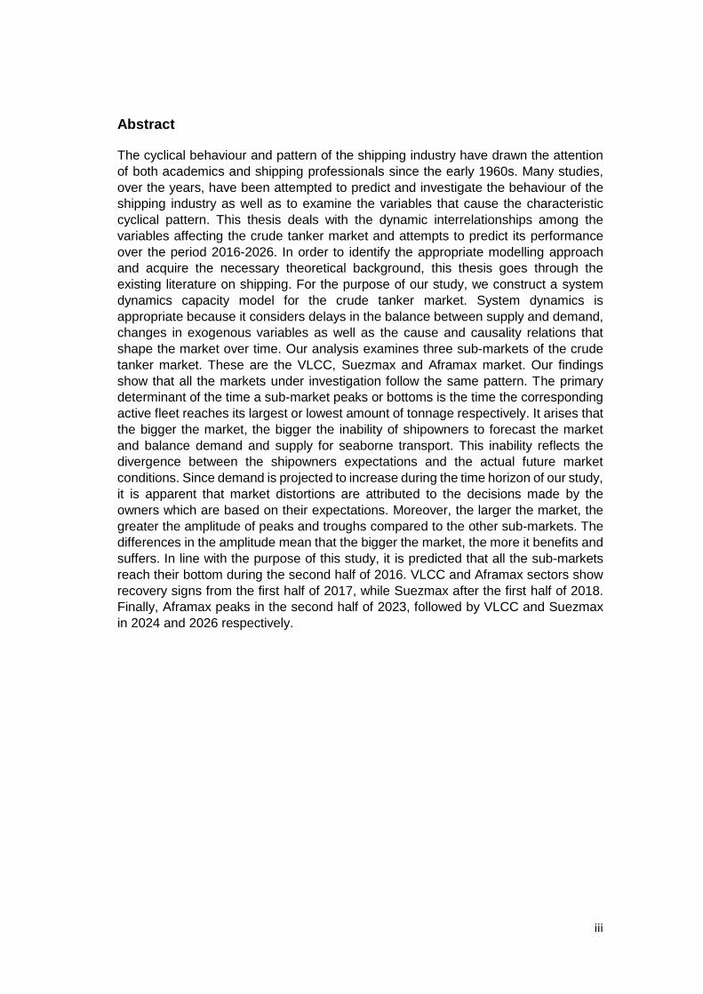
Abstract

The cyclical behaviour and pattern of the shipping industry have drawn the attention

of both academics and shipping professionals since the early 1960s. Many studies,

over the years, have been attempted to predict and investigate the behaviour of the

shipping industry as well as to examine the variables that cause the characteristic

cyclical pattern. This thesis deals with the dynamic interrelationships among the

variables affecting the crude tanker market and attempts to predict its performance

over the period 2016-2026. In order to identify the appropriate modelling approach

and acquire the necessary theoretical background, this thesis goes through the

existing literature on shipping. For the purpose of our study, we construct a system

dynamics capacity model for the crude tanker market. System dynamics is

appropriate because it considers delays in the balance between supply and demand,

changes in exogenous variables as well as the cause and causality relations that

shape the market over time. Our analysis examines three sub-markets of the crude

tanker market. These are the VLCC, Suezmax and Aframax market. Our findings

show that all the markets under investigation follow the same pattern. The primary

determinant of the time a sub-market peaks or bottoms is the time the corresponding

active fleet reaches its largest or lowest amount of tonnage respectively. It arises that

the bigger the market, the bigger the inability of shipowners to forecast the market

and balance demand and supply for seaborne transport. This inability reflects the

divergence between the shipowners expectations and the actual future market

conditions. Since demand is projected to increase during the time horizon of our study,

it is apparent that market distortions are attributed to the decisions made by the

owners which are based on their expectations. Moreover, the larger the market, the

greater the amplitude of peaks and troughs compared to the other sub-markets. The

differences in the amplitude mean that the bigger the market, the more it benefits and

suffers. In line with the purpose of this study, it is predicted that all the sub-markets

reach their bottom during the second half of 2016. VLCC and Aframax sectors show

recovery signs from the first half of 2017, while Suezmax after the first half of 2018.

Finally, Aframax peaks in the second half of 2023, followed by VLCC and Suezmax

in 2024 and 2026 respectively.

iv

Table of Contents

Acknowledgements ............................................................................................................ ii

Abstract ................................................................................................................................ iii

List of Tables ........................................................................................................................vi

List of Figures ......................................................................................................................vi

List of Abbreviations ......................................................................................................... vii

CHAPTER 1 Introduction ................................................................................................... 1

1.1. Background ................................................................................................... 1

1.2. Problem Statement and Research Objectives ................................................ 2

1.3. Research Design ........................................................................................... 4

1.4. Thesis Structure ............................................................................................. 4

Chapter 2 Crude tanker Characteristics and Shipping Markets ............................. 6

2.1. Introduction .................................................................................................... 6

2.2. Types of Crude Oil Tankers and Main Trade Routes ..................................... 6

2.3. Costs of Running a Vessel ............................................................................. 8

2.4. The Four Shipping Markets ............................................................................ 9

2.4.1 Freight Market ...................................................................................................... 9

2.4.2. Newbuilding Market .......................................................................................... 11

2.4.3. Sale and Purchase (S&P) or Secondhand Market ...................................... 12

2.4.4. Demolition Market ............................................................................................ 12

2.5. Summary ..................................................................................................... 13

Chapter 3 Crude Oil Market ............................................................................................ 14

3.1. Introduction .................................................................................................. 14

3.2. Current Crude Oil Market ............................................................................. 14

3.3. Summary ..................................................................................................... 16

Chapter 4 Shipping Cycles ............................................................................................. 17

4.1. Introduction .................................................................................................. 17

4.2. Demand and Supply for Sea Transport Services ......................................... 17

4.3. Characteristics of Shipping Cycle ................................................................. 18

4.4. Summary ..................................................................................................... 20

Chapter 5 Overview of Previous Modelling Approaches ........................................ 21

5.1. Introduction .................................................................................................. 21

5.2. Various Modelling Approaches .................................................................... 21

5.2. System Dynamics (SD) ................................................................................ 23

v

Chapter 6 Methodology and Data ................................................................................. 26

6.1. Introduction .................................................................................................. 26

6.2. Variables Used in the Model ........................................................................ 27

6.3. Data Collection and Structure ...................................................................... 27

6.4. Methodology ................................................................................................ 28

6.4.1. Introductory Comments and Assumptions ................................................... 28

6.4.2. Crude Tanker Industry Dynamics .................................................................. 29

6.4.3. Model Equations ............................................................................................... 30

Chapter 7 Analysis and Results .................................................................................... 35

7.1. Introduction .................................................................................................. 35

7.2. VLCC Market ............................................................................................... 36

7.3. Suezmax Market .......................................................................................... 41

7.4. Aframax Market ........................................................................................... 46

7.5. Overall Crude Tanker Market Analysis ......................................................... 51

Chapter 8 Conclusions and Recommendations ....................................................... 54

8.1. Conclusions ................................................................................................. 54

8.2. Limitations ................................................................................................... 56

8.3. Recommendations for Further Research ..................................................... 56

Bibliography ....................................................................................................................... 57

Appendices ......................................................................................................................... 62

Appendix 1: Vensim Software Model .................................................................. 62

Appendix 2: Initial Fleet 2016 in Million DWT ...................................................... 63

Appendix 3: Initial Orderbook 2016 in Million DWT ............................................. 63

Appendix 4: Annual Scraping Rate Calculations in Million DWT ......................... 63

Appendix 5: Initial Demand 2016 in Million DWT ................................................ 63

Appendix 6: Average Annual Oil Sea Trade Growth in Million Tonnes ................ 64

vi

List of Tables

Table 1: Technical Characteristics and Typical Trade Routes per Crude Oil Tanker

Type ......................................................................................................................... 7

Table 2: Contracts, Responsibilities and Freight Rate Basis ................................... 13

Table 3: Main Factors Affecting Demand and Supply ............................................. 17

List of Figures

Figure 1: International Seaborne Trade 2014 ........................................................... 6

Figure 2: Brent Oil Prices ($/barrel) ........................................................................ 14

Figure 3: World Crude Oil Production (Thousand barrels/day) ............................... 15

Figure 4: World GDP Growth .................................................................................. 15

Figure 5: Stages in Shipping Cycles ....................................................................... 19

Figure 6: The Mechanism of Shipping .................................................................... 26

Figure 7: Market Dynamics ..................................................................................... 29

Figure 8: Model Settings ........................................................................................ 35

Figure 9: Demand for VLCC in Million DWT ........................................................... 36

Figure 10: VLCC Supply in Million DWT ................................................................. 37

Figure 11: VLCC Deliveries in Million DWT ............................................................ 37

Figure 12: VLCC Orders in Million DWT ................................................................. 38

Figure 13: VLCC Orderbook in Million DWT ........................................................... 39

Figure 14: VLCC Market Equilibrium in million DWT ............................................... 39

Figure 15: VLCC Shipowners Forecast Error in Million DWT .................................. 40

Figure 16:Demand for Suezmax in Million DWT ..................................................... 41

Figure 17:Suezmax Supply in Million DWT ............................................................. 42

Figure 18:Suezmax Deliveries in Million DWT ........................................................ 42

Figure 19:Suezmax Orders in Million DWT ............................................................. 43

Figure 20:Suezmax Orderbook in Million DWT ....................................................... 43

Figure 21:Suezmax Market Equilibrium in Million DWT .......................................... 44

Figure 22: Suezmax Shipowners Forecast Error in Million DWT ............................. 45

Figure 23:Demand for Aframax in Million DWT ....................................................... 46

Figure 24:Aframax Supply in Million DWT .............................................................. 47

Figure 25:Aframax Deliveries in Million DWT .......................................................... 47

Figure 26:Aframax Orders in Million DWT .............................................................. 48

Figure 27:Aframax Orderbook in Million DWT ........................................................ 48

Figure 28:Aframax Market Equilibrium in Million DWT ............................................ 49

Figure 29: Aframax Shipowners Forecast Error in Million DWT .............................. 50

Figure 30: Summary of Crude Tanker Market in Million DWT ................................. 51

Figure 31: Summary of Crude Tanker Fleet in Million DWT .................................... 52

Figure 32: Summary of Shipowners Forecast Error in Million DWT ........................ 53

vii

List of Abbreviations

OAPEC-Organization of Arab Petroleum Exporting Countries

BIMCO- Baltic and International Maritime Council

VAR-Vector Auto-regression

FFA-Forward Freight Agreement

FOSVA-Forward Ship Value Agreement

GARCH- Generalized Auto-Regressive Conditional Heteroskedasticity

ADF- Augmented Dickey-Fuller test

PP- Philips Perron test

ESTAR- Exponentially Smooth-Transition Autoregressive model

VEC-Vector Error Correction model

SD-System Dynamics

OPEC-Organization of the Petroleum Exporting Countries

OECD- The Organisation for Economic Co-operation and Development

UNCTAD- United Nations Conference on Trade and Development

IMO-International Maritime Organization

MARPOL- International Convention for the Prevention of Pollution from Ships

DWT- Dead Weight Tonnage

VLCC- Very Large Crude Carrier

ULCC- Ultra Large Crude Carrier

TC-Time Charter

WS-Worldscale

S&P-Sale and Purchase Market

TCE-Time Charter Equivalent

viii

1

CHAPTER 1 Introduction

1.1. Background

Oil tankers are carrying the most valuable commodity of the world, oil. Oil tanker industry is over 100 years old. The need for oil transportation through sea-going vessels arose around 1860 when the industrial activity of Europe was in need of importing oil from the United States. Although the first ever trans-Atlantic sea transport of oil took place with a vessel plying from the USA to Europe, the wooden ship made this shipment is not considered an oil tanker as it transported oil in barrels (Niko Wijnolst, 1999). Cost and utilization issues gave rise to tank ships. The first hull designed tank vessel, named the Glückauf, built in 1886 (Niko Wijnolst, 1999), and is considered the predecessor of the current oil tanker industry.

Oil is the driving force of the global economy as it has been the dominant source of energy. Modern economies depend on oil as global living standards, technology and industrial activity are improving and becoming more demanding with respect to the quantity of energy needed. After that, many countries have been investing in refineries to secure the demanded petroleum products and boost their economy through exports and domestic demand.

Various geopolitical and economic events render oil industry very volatile leading in significant oil shortage and price fluctuations. These fluctuations are the aftermath of changes happening in demand for and supply of oil. The demand for oil transportation is derived demand and thus the performance of oil tanker industry is inevitably affected by the distortions in demand for and supply of oil. Not only these distortions do affect the demand for seaborne transportation but also the operating costs of the vessel as most vessels sailing all over the globe use oil fuel.

Oil has the power to reshape both the global economy and tanker industry. A typical example is the oil crisis in 1973 when oil embargo by the OAPEC was announced as a response to the involvement of the USA in the Arab-Israeli War. At this time the oil price rocketed halting economic growth. This increase in price had a direct impact on oil tanker industry as the demand for oil transportation plunged increasing the lay-up and scrapping levels as well as the operation costs of vessels. The headwinds of oil tanker industry at that time forced many ship owners to send their newbuilding ships directly from the shipyards to scrapping.

Another typical example is since the second half of 2014 when oil price started falling at very low levels reshaping and boosting the oil tanker industry. Since this time to date, the tanker industry has experienced its best performance after the tanker market crash in 2008. The demand for oil transportation and storage has surged at unprecedented levels offering shipowners enormous earnings. Many traders have been purchasing oil with a view to selling it in the future at much higher price. They have been storing oil in tankers waiting idly off main ports in order to meet future demand at a higher price making fortunes from the price gaps, a phenomenon known as “Contango”. Refineries producing petroleum products need oil as feedstock. Thus, refineries all over the world have increased their demand for oil as well as their production levels as their profit margin is much larger because of the low oil price.

2

Through the history of oil tankers various geopolitical and/or economic events has led to the reshaping of the industry. What characterizes the tanker industry as well as the shipping industry in general, is cyclicality and volatility. However, there are auto-correcting driving forces that tend to stabilize the market and bring demand for and supply of tonnage for seaborne oil trade in balance. The purpose of our study is to present these forces and assess the tanker industry in the next ten years.

1.2. Problem Statement and Research Objectives

In the year 2015, the oil tanker market achieved its best performance since 2008

despite the lower growth level of the global economy (BRS, 2016). This performance

is primarily attributed to the free fall of oil price since the second half of 2014 and the

relatively low tonnage supply of oil tankers at the start of oil price slide (BIMCO, 2016).

This slide led to an unprecedented level demand for oil by refineries all over the world.

High margins of oil refineries rocketed the need for oil tankers. A typical example is

the enormous crude oil imports by China which constitute a primary reason for the

high deployment of oil tankers. The low oil price prompted China to build large oil

stocks as the living standards of its citizens have been becoming similar to those of

the developed countries as the China’s social classes have been reformulated. China

has taken advantage of low oil price in order to secure oil reserves for future needs.

However, a question being raised is whether China has reached or approached its

desired levels of oil stocks. It is apparent that, in either case, the market of oil tankers

will be adversely affected in the coming years.

Low oil prices have contributed to the closure of many oil fields, especially in the North

Sea, diminishing their margins and making it for them unfordable to operate, shaking

the global oil supply. On the other hand, the lifting of the USA and Iran sanctions on

exporting oil, in December 2015 and January 2016 respectively, reshapes and alters

both the map and levels of oil production as well as the performance of the tanker

market as new trade routes are emerging. Another menacing problem that the tanker

market faces is the expected huge number of deliveries between the years 2016 and

2017. BIMCO is expecting in the course of 2016 a crude oil fleet growth of 4.5%

highlighting that as the demand will not follow the same direction, there will be

pressure on freight rates (BIMCO, 2016). Since May 2016 we have witnessed a fall

in VLCC freight rates raising concerns around the market professionals about tonnage

oversupply. Even if the market holds forces which auto-correct the market, this

procedure takes time.

Another problem that obviously will affect the tanker market in the future is the global

discussions about energy transition as governments are becoming more and more

concerned about environmental problems. Having started with enforcing strict

regulations on environmental pollution, governments are investing in a huge amount

of money in order to find alternative energy sources and create a cleaner planet.

However, if their projects apply in the distant future, the oil industry will become

obsolete.

It is apparent that oil tanker industry is facing not only temporary but also future

problems. Thus, questions are being raised regarding the medium to long term future

of the market. Is the market entering a state of prolonged decrease in freight rates

because of oversupply or new emerging trade routes will sustain its high

3

performance? How will the crude tanker market perform taking into consideration the

high uncertainty regarding oil price and production levels? How will the market deal

with the uncertainty of global economy and geopolitical tensions? How governments’

projects will affect the market in the future?

Contemplating the volatile nature of the market itself, we believe it is imperative for

the shipping professionals to be examining the market continuously in order to take

the right decisions that mitigate their risk. The scope of this study is to create an

appropriate model that will enable people engaged or interested in the shipping

industry to form an insight of how the crude tanker market will perform in the next ten

years. Thus, in order to achieve our objectives, we need to answer our main research

question:

“How can we quantitatively assess the medium to long-term future of the crude oil

tanker market?”

The idea of our main research question is to understand fully the variables that affect

the performance of the market and cause cyclicality as well as to go through past

works attempting to analyze the market. After doing this, we aim to provide both

professionals and academics with a useful model enabling them to assess the

medium to the long-term performance of the market. To reach our desired outcomes

and answer our central question, we first need to deal with the following series of sub-

questions:

“How is the tanker market structured?”

“What are the factors influencing demand and supply in shipping?”

“What are the characteristics of shipping cycles?”

“How can we construct a system dynamics model for the tanker industry?”

4

1.3. Research Design

This thesis employs both qualitative and quantitative methods in order to answer our

main and sub-research questions. With respect to the first sub-research question, we

will go through the existing literature on shipping so as to define the characteristics of

the crude tankers and analyze the shipping markets with which the tanker industry is

dealing.

Using the same approach for the next two sub-research questions, we aim to define

the factors affecting the supply and demand for transport by sea as well as to

understand their interrelations through which shipping cycles are generated.

Moreover, the existing literature will provide us with the characteristics and definitions

of these cycles.

For the last sub-research question, after going through past papers using system

dynamics approach to modelling the shipping market, we intend to cite the suitability

of system dynamics for the purpose of our study. Then, we are going to explain the

assumptions and structure of the system dynamics model we employ for assessing

the performance of the tanker industry in the next ten years.

1.4. Thesis Structure

In Chapter 2, the main categories of crude tankers and their key features in terms of

size and trade routes are presented. Furthermore, an analysis of the shipping markets

and their importance is conducted. Chapter 2 concludes with a part devoted to the

main costs of running a vessel. By doing so, we want to provide the reader with a

broad view of the tanker industry as we present not only the characteristics of the

industry but also the costs associated with running a crude tanker.

In chapter 3, we analyze the current situation of the crude oil market. An Analysis of

the current crude oil market is crucial as it provides readers with an insight of the

market condition of the main commodity carried by crude tankers.

Chapter 4 is devoted to the factors affecting the supply of and demand for sea

transport as well as the characteristics of shipping cycles and its determinants. The

shipping industry is very volatile and shipping cycles dominate the market. Therefore,

understanding the behavior of the shipping cycles as well as their determinants is vital

for choosing the right modelling approach.

In chapter 5, we present previews modelling approaches of the shipping industry.

Moreover, we devote a section to System Dynamics where we cite past system

dynamics approaches. We conclude the chapter by citing the suitability of System

Dynamics for the purpose of our study.

Chapter 6 deals with the methodology we develop regarding the construction of our

model. First of all, we present the variables which are used as inputs into our model

as well as the dynamic relationships that rule our model. We conclude our

methodology part by presenting all the mathematical equations and necessary

assumptions to construct the model. In turn, Chapter 7 discusses and analyzes the

5

results arising from our model. After analyzing the market conditions and their

determinants for each tanker market separately, we compare the market conditions

among the different sectors in order to draw a conclusion about the performance of

the overall crude tanker market in the next ten years.

Finally, in Chapter 8, we present our conclusions and recommendations for further

research.

6

Chapter 2 Crude tanker Characteristics and Shipping Markets

2.1. Introduction

Over the years, the expansion of shipping industry attracted many players. As a result,

fierce competition has arisen with the free entry and exit of shipowners. The shipping

industry has become a really international business offering asset mobility.

The capital intensive and competitive character of the industry gave rise to many

professions related to shipping. Shipping industry comprises a large group of people

ranging from shipowners to shipbrokers, insurers, bankers, consultants, maritime

lawyers as well as other service providers. It is vital for the competitive advantage of

the professionals involved in the industry to understand the four shipping markets

which, according to Stopford (2009), are integrated together and generate competitive

market conditions. These four markets are the freight market, newbuilding, sale and

purchase (S&P) or secondhand and demolition. In this chapter, we analyze the types

of crude oil tankers and costs incurred in shipping as well as the structure of the

shipping markets in order to give the reader a broad view of the oil tanker industry.

2.2. Types of Crude Oil Tankers and Main Trade Routes

There are two basic sub-categories of oil tankers, the crude oil and product tankers.

According to UNCTAD’s review of maritime transport 2015, in 2014, the volume of

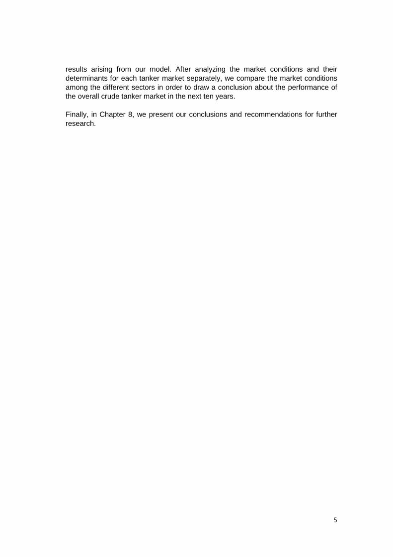
seaborne trade was responsible for nearly four-fifths of the world’s trade totaling to

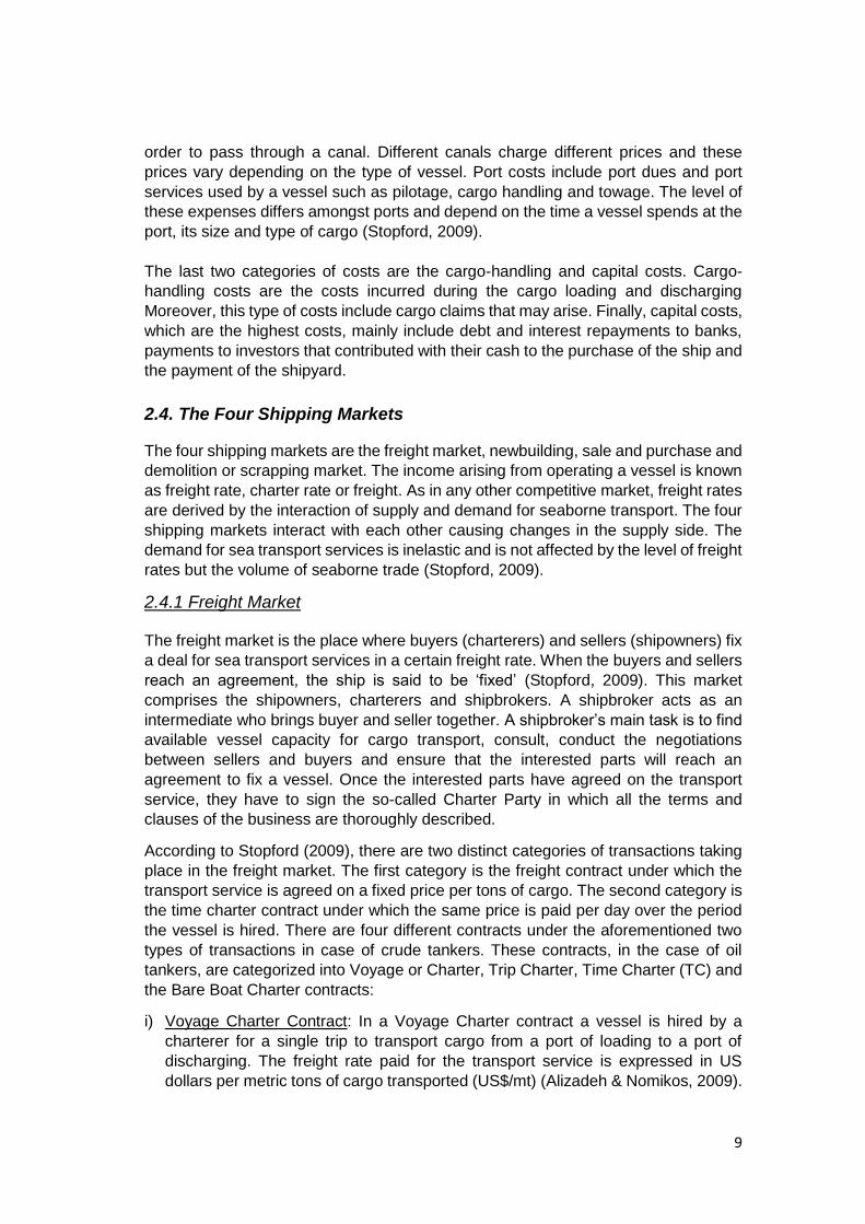
9.84billions of which crude oil tankers accounted for 17% (Figure 1), while product

tankers for 9% respectively (UNCTAD, 2015). These two types of merchant ships are

used for the seaborne bulk transport of oil. Crude oil tankers carry unrefined crude oil

from crude producing points to refineries all over the world. On the other hand, product

tankers, similar to crude oil tankers but smaller in size, are responsible for the

seaborne bulk transportation of clean and dirty oil products derived from the process

of crude oil. However, this research focuses on crude oil tankers and so we are not

going to elaborate further on product tankers.

Figure 1: International Seaborne Trade 2014 Source: Compiled by author via UNCTAD secretariat, based on Clarksons

Research, Seaborne Trade Monitor, 2(5), May 2015

7

In the past, crude tankers were designed with a single hull. To prevent the likelihood

of oil spills in the event of an accident, such as in the case of Exxon Valdez in 1989,

IMO introduced measures to ensure that tankers are constructed under certain

specifications. MARPOL 1992 provides that all the vessels ordered after the 6th of July

1993 should be designed and built with double hulls as well as that old ships designed

with single hull should be taken out after a certain age (International Maritime

Organization IMO, 2016).

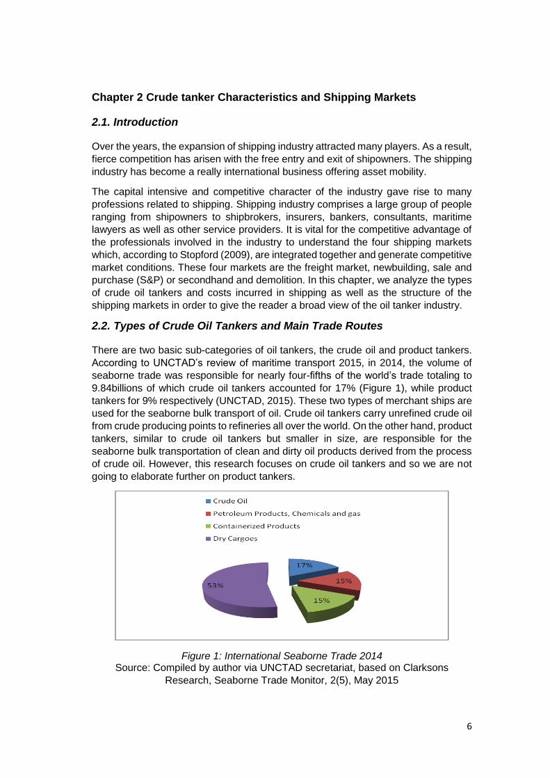
Crude tankers are subdivided into five main categories according to their size in dead

weight tonnage1 (dwt), the market and the regions they can safely operate. Their size

varies ranging from 60,000 dwt to over 200,000 dwt. Crude tankers are categorized

into Panamax, Aframax, Suezmax, Very Large Crude Carries (VLCC) and Ultra Large

Crude Carriers (ULCC). The latter two are known as supertankers.

Panamax is the largest ship that can pass through the Panama Canal, while Suezmax

is the maximum size of a tanker that can cross the Suez Canal. Aframax tankers are

suitable for short and medium oil transportation routes and their favourable size allow

them to reach and serve most ports around the world. Finally, VLCCs and ULCCs,

transporting huge amounts of crude oil, serve the biggest ports in the world as well as

offshore terminals. The draft2 and size of these two types restrict the routes and ports

they can operate. In Table 1 below, we summarize the main characteristics of each

crude tanker category.

Table 1: Technical Characteristics and Typical Trade Routes per Crude Oil Tanker Type

Type dwt Typical Draft

Typical Length

(meters)

Typical Trade Routes

Panamax 60,000-79,999 13.7 228 Intra-regional locations

Aframax 80,000-119,999 14.8 244 From West Africa to U.S. and Europe.

This type also serves intra-regional

locations Suezmax 120,000-199,999 17 274 Atlantic Basin

(Transporting crude from the North Sea,

West Africa and Russia)

VLCC 200,000-319,999 21 333 From the Arabian Gulf to Western

1 The Dead Weight Tonnage (dwt) measures a vessel’s carrying capacity in tons including fuels, water, provisions and crew. This measure excludes a vessel’s weight.

2 The draft of a vessel is the vertical distance between the vessel’s lowest point and the water line.

8

Europe, U.S. and Asia

ULCC 320,000 and above

24.5 380 From the Persian Gulf to Europe, North

America and Asia

Source: Compiled by the author via various sources

2.3. Costs of Running a Vessel

There are various costs associated with the running of a ship. Shipping companies

spend huge amounts of money in order to fully equip and meet the needs of a vessel,

while at sea or port. The major cost categories of a bulk ship are the operating costs,

periodic maintenance, voyage costs, cargo-handling costs and capital costs

(Stopford, 2009). The biggest costs are the operating, voyage and capital costs

accounting for about 14%, 40% and 42% of the overall costs respectively (Stopford,

2009).

The operating costs are associated with the daily expenses of running a ship

excluding fuels, which are part of the voyage costs. The crewing of the vessel

accounts for 50% of the operating costs and includes costs relating to wages and

salaries, crew insurance and pension, training, victuals and travelling (Stopford, 2009)

. Additional costs arising from the daily operation of a vessel are the need for stores

and consumables, repairs and maintenance, insurance and other general costs

(Stopford, 2009). Stores and consumables are expenditures relating to lubricants and

storage of various items needed and consumed aboard. Repair and maintenance

include all the necessary maintenance of the vessel’s engine and auxiliary equipment

as well as the necessary ship repairs to meet the vessel specifications described in

the contracts for sea transport services. Insurance costs are the money spent to

insure the vessel against all types of risks such as physical loss or damage to the

ship, cargo damage, collision and environmental pollution. Finally, general costs

include a registration fee to the flag state as well as administrative and management

expenses.

The periodic maintenance cost category includes the expenses for dry docking3

(every two years) and special surveys (every four years) which certify the

seaworthiness and secure the insurance of a vessel (Stopford, 2009). These costs

are becoming higher with the aging of a ship.

Voyage costs are the variable costs incurred under a specific voyage. These costs

are divided into fuel or bunker costs, canal dues and port costs. Bunker or fuel costs

account for about 50% of the voyage costs and the amount of such costs depends on

the engine design, the age of the ship as well as the type of the fuel oil. Based on

their quality and specific characteristics such as level of Sulphur dioxide, fuel oils are

classified, into Marine Gas Oil (MGO), Marine Diesel Oil (MDO), Intermediate Fuel Oil

(IFO) and Heavy Fuel Oil (HFO). Canal dues are the tolls imposed on a vessel in

3 Dry docking means that a ship is brought onto dry land in order to be repaired or inspected.

9

order to pass through a canal. Different canals charge different prices and these

prices vary depending on the type of vessel. Port costs include port dues and port

services used by a vessel such as pilotage, cargo handling and towage. The level of

these expenses differs amongst ports and depend on the time a vessel spends at the

port, its size and type of cargo (Stopford, 2009).

The last two categories of costs are the cargo-handling and capital costs. Cargo-

handling costs are the costs incurred during the cargo loading and discharging

Moreover, this type of costs include cargo claims that may arise. Finally, capital costs,

which are the highest costs, mainly include debt and interest repayments to banks,

payments to investors that contributed with their cash to the purchase of the ship and

the payment of the shipyard.

2.4. The Four Shipping Markets

The four shipping markets are the freight market, newbuilding, sale and purchase and

demolition or scrapping market. The income arising from operating a vessel is known

as freight rate, charter rate or freight. As in any other competitive market, freight rates

are derived by the interaction of supply and demand for seaborne transport. The four

shipping markets interact with each other causing changes in the supply side. The

demand for sea transport services is inelastic and is not affected by the level of freight

rates but the volume of seaborne trade (Stopford, 2009).

2.4.1 Freight Market

The freight market is the place where buyers (charterers) and sellers (shipowners) fix

a deal for sea transport services in a certain freight rate. When the buyers and sellers

reach an agreement, the ship is said to be ‘fixed’ (Stopford, 2009). This market

comprises the shipowners, charterers and shipbrokers. A shipbroker acts as an

intermediate who brings buyer and seller together. A shipbroker’s main task is to find

available vessel capacity for cargo transport, consult, conduct the negotiations

between sellers and buyers and ensure that the interested parts will reach an

agreement to fix a vessel. Once the interested parts have agreed on the transport

service, they have to sign the so-called Charter Party in which all the terms and

clauses of the business are thoroughly described.

According to Stopford (2009), there are two distinct categories of transactions taking

place in the freight market. The first category is the freight contract under which the

transport service is agreed on a fixed price per tons of cargo. The second category is

the time charter contract under which the same price is paid per day over the period

the vessel is hired. There are four different contracts under the aforementioned two

types of transactions in case of crude tankers. These contracts, in the case of oil

tankers, are categorized into Voyage or Charter, Trip Charter, Time Charter (TC) and

the Bare Boat Charter contracts:

i) Voyage Charter Contract: In a Voyage Charter contract a vessel is hired by a

charterer for a single trip to transport cargo from a port of loading to a port of

discharging. The freight rate paid for the transport service is expressed in US

dollars per metric tons of cargo transported (US$/mt) (Alizadeh & Nomikos, 2009).

10

Under such a contract, shipowners have the full control and management of their

vessels and are responsible for both the nautical control of the vessel and the costs

incurred during the voyage. These costs are categorized into the voyage,

operating, cargo handling and capital costs as shown and are analyzed in a later

section in this chapter. The voyage and trip charter consist the so-called spot

market. Spot market refers to contracts signed for single or short-term (maximum

duration of three months) consecutive voyage/trips (maximum duration of three

months).

Oil tanker voyage contract freights are calculated based on an international freight

index called Worldscale (WS). The Worldscale Association reports, usually each

year, the WS100 which is the basis for freight rate negotiations. The corresponding

WS 100 for a specific voyage, which is expressed in US$/mt, is the freight rate

arising after calculating the costs incurred by operating a standard 75,000dwt

Aframax vessel in a particular round-trip (Alizadeh & Nomikos, 2009). The WS 100,

which is also known as Worldscale flat rate, is the break-even for a specific voyage.

(Alizadeh & Nomikos, 2009). The freight rate negotiated in a voyage contract is a

percentage rate of WS 100. For instance, WS 175 means that the agreed freight

rate is 175% of the reported WS 100, while a WS 75 is the 75% of the WS 10

(Worldscale Association, 2016).

ii) Trip Charter Contract: A vessel is hired by a charterer for a specified trip or period

of maximum three months and the price is fixed per day (US$/day). The price is

based on the so-called Time Charter Equivalent and (TCE). Under a trip charter

contract, shipowners have the management and operational control of the vessel.

The main advantage over the voyage charter is that voyage costs are paid by the

charterer and shipowner is paid for any voyage delay as the charge of the providing

transport service is a fixed price in US$/day.

iii) Time Charter (TC) Contract: Under a Time Charter contract a charterer hires a

vessel for a specified time ranging from few months (three months and above) to

several years. The agreed freight rate is fixed and expressed in US$/day. The

charterer has the operational control of the vessel and covers the voyage costs

incurred during the period of the contract. On the other hand, the shipowner has

the management of the vessel and is responsible for the operating as well as the

capital costs of the vessel. The advantage of this type of contract over a voyage

contract is that the shipowner secures stable revenues for a specified period and

avoid the voyage costs.

iv) Bare Boat Charter Contract: This type of contract is preferred by the charterers

when they want to have the full control and management of the vessel. The period

of such a contract usually spans between ten and twenty years. Over this period,

the owner of the vessel receives a fixed freight, usually in US$/day. The charterer

is responsible for all the costs except for the capital costs which are paid by the

owner of the vessel. Typically, the owner of the asset is a financial institution

without expertise in shipping industry (Stopford, 2009).

11

2.4.2. Newbuilding Market

The newbuilding market is the market dealing with the orders and deliveries for new

vessels. Shipbuilding requires great investments and thus, the negotiations can be

tough and time-consuming. Therefore, often, shipbrokers are hired to execute the

negotiations and bankers to secure the money for the investment. The main talks

focus on the price of the vessel, vessel specifications, source of finance of the

investment as well as the contract terms and conditions (Stopford, 2009).

Shipowners place orders for new ships either to increase their existing fleet or replace

the old ones with more efficient ships, equipped with advanced technologies and

designed to meet the growing regulations enforced in the industry. The time between

the placement of an order and delivery of a new ship can range from 1 to 2 year. In

general, the factors affecting the shipbuilding activity are the freight rates, shipbuilding

costs, aging of existing fleet and international regulations. There is a positive

correlation between the volume of orders and freight rates, but negative between the

shipbuilding activity and the shipbuilding costs.

The number of vessels ordered reflects the expectations of shipowners regarding the

growth of seaborne trade and the level of future freight rates. When demand overtakes

supply for seaborne trade, shipowners expect high freight rates and thus, they order

new vessels to stabilize the market and take advantage of the high revenues.

Consequently, it is apparent that the shipbuilding activity is unpredictable as it

depends on shipowners’ behavior, decisions and expectations. Therefore, the overall

market sentiment can boost the shipbuilding activity to such a level that lead to vessel

oversupply and low freight rates. The depressed market can last for a long time as

the average lifespan of new vessels is 25 years. The market recovers in the long run

when ships are scrapped (see section 2.4.4.) and supply reaches again the demand.

Considering all these, it is obvious that the newbuilding market governs the shipping

market causing fluctuation in freight rate levels.

Shipbuilding prices move together with the shipbuilding activity. The more the

shipowners order, the more the prices rise. When the freight market moves

downwards, shipowners are not interested in ordering new vessels. As the orderbook

decreases, shipbuilding prices can drop to very low prices because of the depressed

market. On the other hand, in market booms the prices are skyrocketed as orders

increase.

12

2.4.3. Sale and Purchase (S&P) or Secondhand Market

The tanker freight market is the market where shipping companies generate

revenues. When demand for seaborne trade is high, the owners seek to buy vessels,

either in the Sale and Purchase or Newbuilding market, to expand their business. The

Sale and Purchase market, known as S&P, deals with the sale and purchase of

secondhand vessels. In this market, tens of millions of dollars are traded in the blink

of an eye. Only in 2006, 1,500 secondhand merchant ships were sold for $36billion in

total (Stopford, 2009). The so-called S&P shipbrokers are usually hired to execute the

negotiations and transactions of sales and purchases.

The S&P and Newbuilding markets deal with the same type of asset and thus, owners

step into one of these markets depending on their needs. While the delivery of a new

building vessel requires 1 to 3 years since the placement of the order, the delivery

time of a secondhand ship is much shorter. According to Goulielmos (2009), when

the oil tanker market thrives, the owners can promptly increase their volume to meet

the demand for oil transport services by purchasing tankers from the S&P market.

The Secondhand market is considered as an auxiliary market as the number and

carrying capacity of the existing ships does not change with the purchase or sale of a

secondhand vessel (Strandenes, 2002). Therefore, S&P market itself does not affect

the freight market when there is no delivery of new building ships and/or scrapping

activity. In general, secondhand market enables owners to exit the shipping market

or restructure their fleet depending on changes in the demand for shipping services

(Strandenes, 2002).

The main factor affecting the price of secondhand vessels is freight rates. Moreover,

secondhand prices are affected by the age of the vessel, inflation and expectations

regarding the market. Prices follow the same direction as freight rates. This fact

makes it clear that second-hand market is very volatile. The second most important

influence in prices is the expectations of the market. In the case investors foresee that

freight rates will go up, the demand for used ships increases followed by a

corresponding rise in prices. When market thrives, the demand for used ships

increases to such a level that prices can reach that of newbuildings. Similarly, when

the market is in recession, the prices of used ships are plummeting and reach that of

scrapping.

Finally, each single sale taking place in the market set a benchmark with respect to

the price of the type of ship sold. Therefore, price negotiations of prospective sales

are based on this benchmark.

2.4.4. Demolition Market

The last shipping market is the demolition market. This market deals with obsolete

and old vessels. Along with the newbuilding market, demolition market determines

the capacity of ships available to serve the existing demand for sea transport services

(Strandenes, 2002).

Shipowners are forced to scrap part of their fleet in case vessels do not meet the

existing regulations and safety requirements or the costs of running a vessel exceed

freight rates. By scrapping ships, owners expect a financial return to counterbalance

13

their loss from operating a vessel in a market in recession or to increase their capital

by obsolete ships which are at the end of their life. However, when there is a boom

market, the owners are reluctant to scrap ships as they experience high freight rates.

In such a market, the owners deploy vessels even of 30 years old. It is apparent that

there is a relationship between the secondhand and demolition market as the ships

brought to scrapping are the old and used vessels which consist the S&P market.

The buyers of ships for scrapping are the demolition or ship breaking yards with the

most ship breaking activity taking place in the Far East. Leaders in ship breaking are

India, Pakistan, China and Bangladesh. Special brokers dealing with the demolition

marketing are hired to conduct the negotiations and set the scrapping price. According

to Knapp et al. (2008) the prices increase with the rise in demand for steel. Another

factor affecting the determination of the price is the number of ships available for

scrapping. If the availability of ships for scrapping decrease then prices increase,

otherwise prices go down.

2.5. Summary

Crude oil tankers are classified into five categories depending on their size and the

routes they serve. The categories of crude tankers by size series are Panamax,

Aframax, Suezmax, VLCC and ULCC. However, to run a vessel there are various

costs incurred. These costs are divided into operating, voyage, cargo-handling and

capital costs as well as periodic maintenance with the voyage and capital costs

accounting for 40% and 42% of the overall costs respectively.

The shipping market consists of four sub-markets, the Freight, Newbuilding, Sale and

Purchase (S&P) and Demolition market. These markets interact with each other

forming the freight levels which reflect the shipping market conditions. The freight

market is the market where buyers and sellers of sea transport services meet to

negotiate and agree on freight rates and terms of the service provided. There are four

different contracts signed in the tanker freight market with differences in duration,

payment basis and responsibilities between the parts involved in a contract (Table 2).

The newbuilding and demolition markets are determinants of the freight rates as these

markets affect the level of tonnage supplied. The newbuilding market deals with the

supply of new vessels, while demolition market is the market where shipowners scrap

their old and obsolete ships. Finally, the S&P market is considered an auxiliary market

as the volumes of sale and purchase of used vessels does not affect the supply of

ships.

Table 2: Contracts, Responsibilities and Freight Rate Basis

Contract Voyage Costs paid

by

Operating Costs paid by

Capital Costs paid

by

Freight rate

Voyage Charter Owner Owner Owner $/ton or WS

Time Charter Charterer Owner Owner $/day

Trip Time Charter

Owner Owner Owner $/day

Bareboat Charter

Charterer Charterer Owner $/day

Source: Compiled by author via various sources

14

Chapter 3 Crude Oil Market

3.1. Introduction

Crude tankers carry the world’s most valuable commodity. Oil is the driving force of

the global economy and growth since it has been the primary energy source and raw

material for almost most of the products we use in our daily life. The crude oil market

is affected by various geopolitical and economic events such as wars, embargoes and

economic crisis reflected in oil production and price level. Such disturbances have a

direct impact on demand for oil and thus, on the demand for crude oil transport and

costs of operating a vessel. In this section, we aim to give an overview of the current

crude oil market.

3.2. Current Crude Oil Market

The top five oil producers by country are U.S., Russia, Canada, Saudi Arabia and

China. Global Oil producers are divided into the so-called OPEC and non-OPEC

countries with OPEC member countries accounting for 40% and 60% of the world’s

crude oil production and exports respectively (U.S. Energy Information Administration,

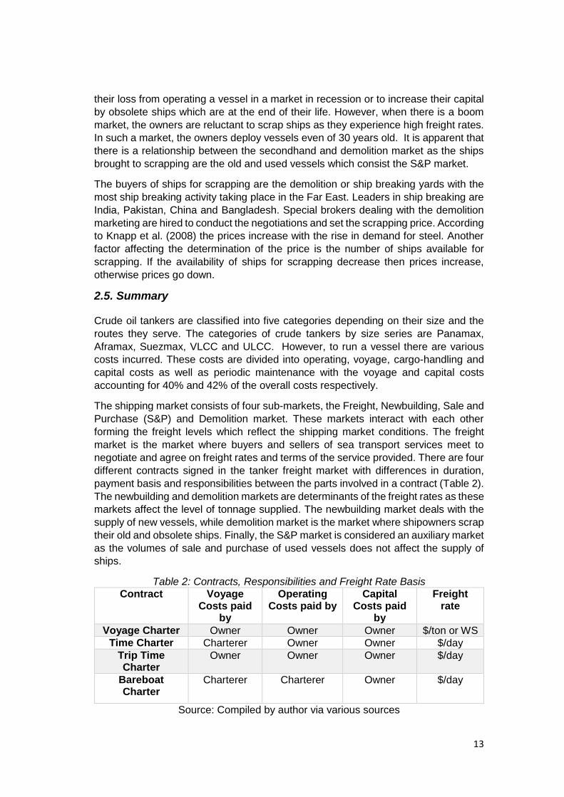
2016). It is evident that OPEC’s production levels have a strong influence on oil prices

due to the law of supply and demand. However, although the market is in distress

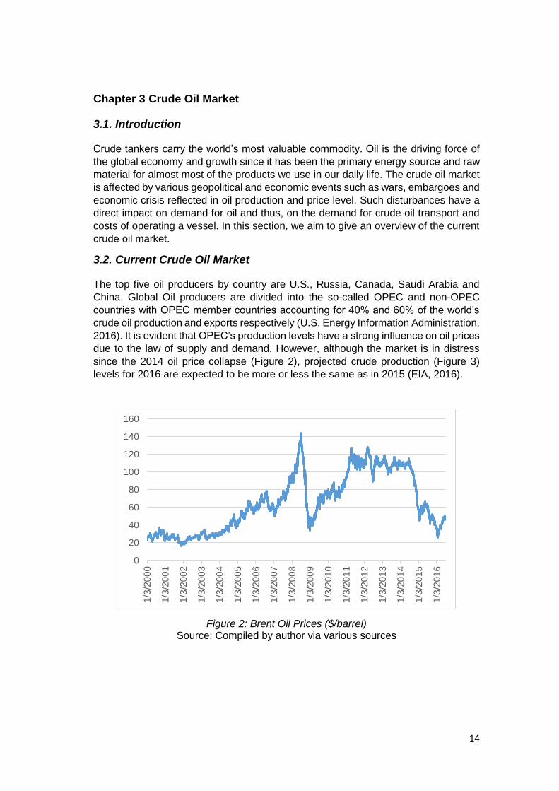
since the 2014 oil price collapse (Figure 2), projected crude production (Figure 3)

levels for 2016 are expected to be more or less the same as in 2015 (EIA, 2016).

Figure 2: Brent Oil Prices ($/barrel) Source: Compiled by author via various sources

0

20

40

60

80

100

120

140

160

1/3

/20

00

1/3

/20

01

1/3

/20

02

1/3

/20

03

1/3

/20

04

1/3

/20

05

1/3

/20

06

1/3

/20

07

1/3

/20

08

1/3

/20

09

1/3

/20

10

1/3

/20

11

1/3

/20

12

1/3

/20

13

1/3

/20

14

1/3

/20

15

1/3

/20

16

15

Figure 3: World Crude Oil Production (Thousand barrels/day) Source: Compiled by author via EIA (EIA BETA, 2016)

After the 50% plummet of oil price in 2014, because of the global crude oversupply,

marginal profits for oil fields have declined and many oil rigs especially, in the North

Sea, have been facing bankruptcy. This price drop urged OPEC members, over the

course of 2016, trying to reach consensus on an oil production freeze to help price

rebound and reach levels before the initiation of the oil price crisis. Furthermore,

around 25 percent of the current platforms in the North Sea could be scrapped

between 2019 and 2026 because of the ageing and mainly, as a result of the low

commodity price since the operating and maintenance costs are not affordable (The

guardian, 2016).

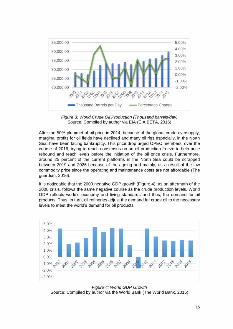
It is noticeable that the 2009 negative GDP growth (Figure 4), as an aftermath of the

2008 crisis, follows the same negative course as the crude production levels. World

GDP reflects world’s economy and living standards and thus, the demand for oil

products. Thus, in turn, oil refineries adjust the demand for crude oil to the necessary

levels to meet the world’s demand for oil products.

Figure 4: World GDP Growth Source: Compiled by author via the World Bank (The World Bank, 2016)

-2.00%

-1.00%

0.00%

1.00%

2.00%

3.00%

4.00%

5.00%

60,000.00

65,000.00

70,000.00

75,000.00

80,000.00

85,000.00

Thousand Barrels per Day Percentage Change

-3.0%

-2.0%

-1.0%

0.0%

1.0%

2.0%

3.0%

4.0%

5.0%

16

The factors determining the crude oil price are the supply and demand for crude oil,

OPEC’s level of production/capacity and various geopolitical events and oil shocks

(IHS, 2014). The latter two affect the supply of crude oil severely, rocketing oil prices.

Another impact on oil prices is the high demand for oil from China, India and at a lower

extent, from other newly industrialised economies (Hamilton, 2008).

China has been a traditional crude oil producer. However, China lowered its

production and increased its imports of crude oil. It has been establishing domestic

refineries to produce oil products to take advantage of its people high needs in oil

products and benefit from the refineries’ huge profit margins since 2014. In the first

half of 2016, China’s crude oil production fell 4.6% (Bloomberg News, 2016). To

conclude, although China was the primary driver for non-OECD countries and global

oil demand growth over the last ten years, India is the first one in 2015 (Sen & Sen,

2016).

3.3. Summary

In this chapter, we attempted to introduce briefly our study’s readers the current

situation in the crude oil market as the demand for crude tankers is derived from the

global oil demand. Finally, we devoted the last paragraph to the main drivers

contributed to the excellent performance of the crude tanker industry since 2014 to

date, naming China and India. It is characteristic of the oil market that the increasing

glut of oil drives oil prices to long-term low levels. On the other hand, developing

countries increase their demand for oil as their living standards become similar to that

of the developed ones. The combination of low oil prices and increasing demand for

oil by developing countries leads to higher demand for oil seaborne transport.

17

Chapter 4 Shipping Cycles

4.1. Introduction

The shipping market is very volatile. Recurrent shipping cycles are dominant in the

history of the shipping industry. Each of these cycles is unique and generated by the

imbalance between supply and demand for sea transport services which in turn cause

fluctuations in freight rates. Shipowners distort the supply side of the market in the

way they behave and react to freight rates. On the other hand, world economy and

various geopolitical events cause fluctuations in demand side (seaborne trade). The

aim of this chapter is to describe the characteristics of shipping cycles after briefly

explaining the factors affecting supply and demand.

4.2. Demand and Supply for Sea Transport Services

The imbalance between supply and demand for sea transport services leads to freight

rates fluctuations. These fluctuations are caused by disturbances in the factors

affecting supply and demand. In Table 3 below, we present the main factors according

to Stopford (2009).

Table 3: Main Factors Affecting Demand and Supply

Demand Supply

The World Economy World Fleet

Seaborne Trade Fleet Productivity

Average Haul Newbuilding Activity

Random Shocks Scrapping Activity

Transport Costs Freight Rates

Source: Compiled by author via Stopford (2009)

Demand

The demand for ships is measured in ton-miles and equals the volume of seaborne

trade (tons) times the average haul (miles) (Stopford, 2009). The average haul is the

average distance of the active sea routes used in order to export and import a specific

cargo. The average haul is influenced by random shocks, such as wars or closure of

Suez or Panama Canal, which increase the distance needed to transport the cargo

because of the difficulties raised. Another factor that can lead to average haul rise is

mistakes in navigation. Therefore, it is obvious the rise in the distance increases the

demand for ships, while the supply falls.

The most important determinant of the demand, however, is the world economy. As

the economy grows along with the living standards, there is an increase in product

consumption and thus, seaborne trade increases. However, the world history has

taught us that random shocks are unpredictable but happen often. For instance, an

economic crisis or a sharp drop or increase in oil prices affect the world economy and

in turn, the demand for seaborne trade. Low oil prices accelerate the world economy

growth, while high prices decelerate it. Thus, it is apparent that decrease in oil prices

raise the demand for crude seaborne trade.

In the past, sea transport was very expensive. However, over the last century,

developments in the shipping industry reduced significantly the costs of transporting

18

cargo by sea. Nowadays, the seaborne transport costs are negligible as technological

advantages led to large and more efficient vessels.

Supply

The supply side is measured in ton-miles and equals the world fleet times the fleet

productivity (Stopford, 2009). The world fleet is affected by the behavior and decisions

made by shipowners in the shipping markets in response to freight rates (see section

2.4.). Fleet productivity measures the performance of active merchant fleet and is

affected by the days a ship is loaded at sea, its speed and deadweight utilization as

well as the time it spends at ports (Stopford, 2009). The more time a ship spends at

ports and sea unloaded, the less productive it is. On the other hand, an increase in

speed and the days a ship is loaded at sea increases its productivity.

Another factor that influences the supply side is the number of ships used for product

storage. This phenomenon, known as Contango, is very common within the oil tanker

industry. Cheap oil is stored by traders in tankers with a view to sell it at a higher price

in the future. Until the traders sell the product, these tankers are out of the market. It

is obvious, that sometime in the future these vessels will be released flooding the

market with excess tonnage which in turn will push freights down.

4.3. Characteristics of Shipping Cycle

Shipping cycles are caused by imbalances in demand and supply. There is much

debate over the factors generating shipping cycles. It is commonly said by shipowners

that cyclicality and volatility in shipping are due to exogenous, unpredictable variables

which affect the demand. They state that global economy and various geopolitical

events are responsible for upturns and downturns in the market. In contrast, maritime

economists agree that both endogenous and exogenous factors shape the cycles

(Abouarghoub, et al., 2012).

The irrational ordering behaviour and over reaction of investors to freight rate signals

distort the market. According to Koopmans (1939), the main determinant of cyclical

patterns in freight rates is the delay in new vessel deliveries. Investors increase orders

based on market conditions or expectations. Upon the deliveries, the market may

have been in recession. Thus, the additional tonnage entering the market could

deteriorate the market further.

Shipping cycles have been dominant in the shipping market. According to Stopford

(2002), endogenous factors trigger the shipping cycles, while the exogenous ones

generate the cyclical pattern. The most important factor that affects demand and thus,

responsible for the cyclical pattern, is the world economy. The business cycles that

govern the world economy generate the shipping cycles, while delays in balancing

supply and demand maintain their intensity (Stopford, 2002). There are three different

types of shipping cycles, the long, short and seasonal cycles (Stopford, 2009).

The long cycle is generated by long-term developments in technology as well as

changes in society and global political scene. The time horizon of this type of cycles

is 20 to 50 years and are not easily detectable (Stopford, 2009). However, the

shipping industry’s long-cycles usually last 20 years as the new vessels entering the

market are not destined to be scrapped before they reach their average lifetime, which

19

is twenty to twenty-five years. Also known as business cycles and much shorter in

duration than long cycles, the short cycles are the most common ones in shipping.

Such cycles are noticeable and their duration can vary since the ordering activity of

the investors, in anticipation to future boom market, can bring the market back to long

recession after a slight recovery. Thus, the time horizon depends on owners’

decisions and can range from 3 to 12 years (Stopford, 2009). Lastly, the seasonal

cycles show fluctuations in freights caused by seasonal variations in demand within a

year. A prominent example is a high mobility of oil tankers in autumn and winter during

which oil is stored to meet the peak demand for oil in winter.

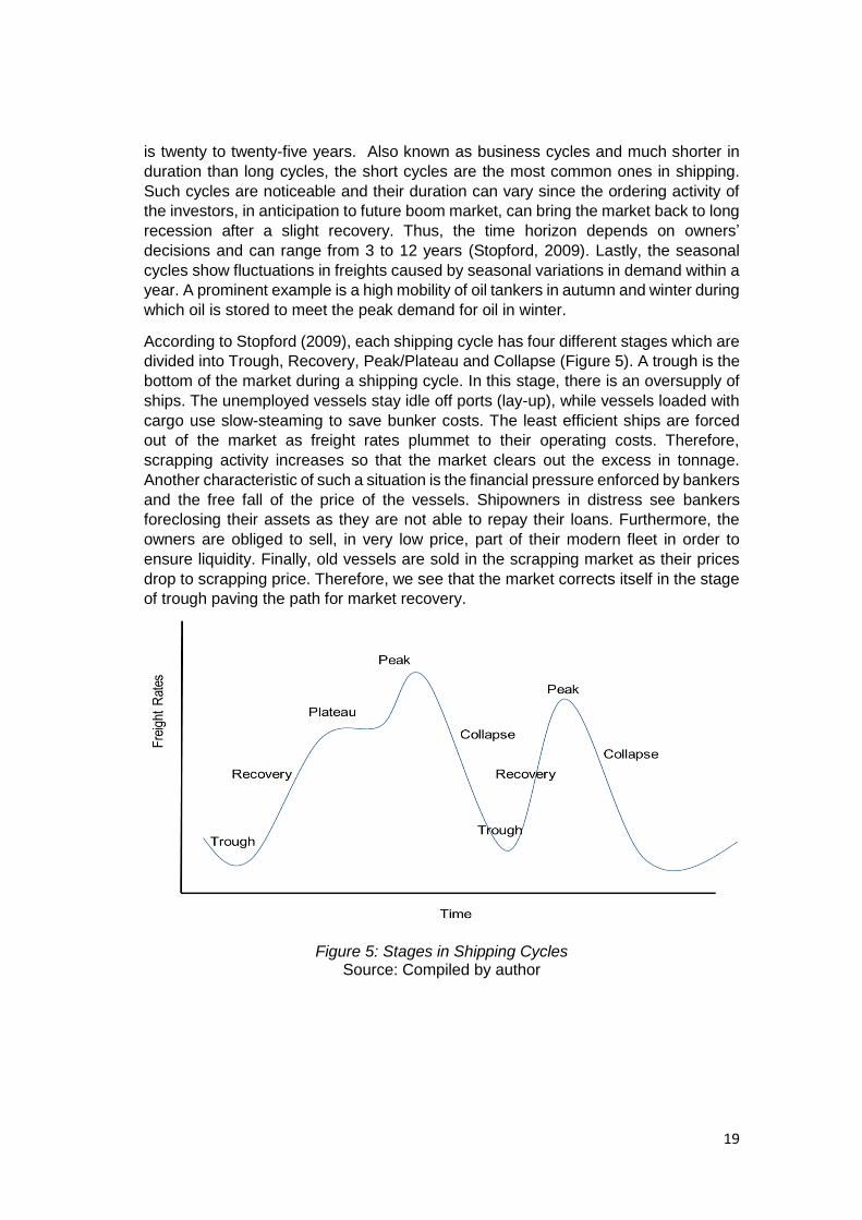
According to Stopford (2009), each shipping cycle has four different stages which are

divided into Trough, Recovery, Peak/Plateau and Collapse (Figure 5). A trough is the

bottom of the market during a shipping cycle. In this stage, there is an oversupply of

ships. The unemployed vessels stay idle off ports (lay-up), while vessels loaded with

cargo use slow-steaming to save bunker costs. The least efficient ships are forced

out of the market as freight rates plummet to their operating costs. Therefore,

scrapping activity increases so that the market clears out the excess in tonnage.

Another characteristic of such a situation is the financial pressure enforced by bankers

and the free fall of the price of the vessels. Shipowners in distress see bankers

foreclosing their assets as they are not able to repay their loans. Furthermore, the

owners are obliged to sell, in very low price, part of their modern fleet in order to

ensure liquidity. Finally, old vessels are sold in the scrapping market as their prices

drop to scrapping price. Therefore, we see that the market corrects itself in the stage

of trough paving the path for market recovery.

Figure 5: Stages in Shipping Cycles Source: Compiled by author

20

During the recovery, freight rates start rising as supply levels approach demand

levels. Laid up vessels start re-entering the market as revenues exceed operating

costs and confidence starts growing. Additionally, both liquidity and prices of used

ships increase gradually.

At the peak/plateau point, during which the market thrives, there is a balance between

demand and supply or shortage of available tonnage. All the fleet in the market is

employed and sails at full speed. Freight rates are skyrocketed. On rare occasions,

freights can be ten times the operating costs (Stopford, 2009). The time horizon of

the peak ranges from weeks to years, depending on the balance between supply and

demand (Stopford, 2009). Bankers are willing to lend money for new or used ships as

they expect high returns from interest rates. Therefore, as lending increases,

newbuilding and S&P activity rises. Secondhand modern ships cost almost the same

or even more than the price of a newbuilding since the demand for ships increases

as investors want to take advantage of the high earnings as fast as possible. Orders

for new vessels increase rapidly leading to market collapse.

The stage of collapse is initiated when tonnage supply overtakes demand. In this

phase, freight rates start falling sharply and confusion pervades the market. This

market turning point can be attributed to the nature of the business cycle, but mostly

is generated by the lag-time of the delivery of new vessels, the world economy and

associated shocks as well as other geopolitical events. The most efficient vessels are

hired and the rest wait in the queue looking for cargo. Shipowners reduce the

operating speed of their vessels as their profit margins decrease.

4.4. Summary

The recurrent shipping cycles make shipping industry very volatile and risky. It is

important for people engaging in shipping to understand fully the factors that create

and reinforce this cyclical pattern in order to mitigate their risk. The cycles are

generated by imbalances between supply and demand. These imbalances can be

attributed to changes in world economy and various geopolitical events as well as to

the irrational behavior of shipowners in response to price signals and the delay of new

deliveries. There are three categories of cycles, the long, short and seasonal cycles.

The most common cycle referred to shipping cycle is the short cycle. The shipping

cycles have four distinct stages which are divided into the Trough, Recovery,

Plateau/Peak and Collapse. Since each stage has its own characteristics, shipping

professionals should examine the market continuously to take the right decisions and

improve the performance and operations of their fleet.

21

Chapter 5 Overview of Previous Modelling Approaches

5.1. Introduction

This chapter aims to provide the reader with a brief overview of previous modelling

approaches and argue the suitability of system dynamics approach for the purpose of

this study.

5.2. Various Modelling Approaches

Shipping freight market has drawn the attention of both professionals and academics since the early 1960s. Norman (1979) investigates the relationship between demand for shipping and measures of economic activity. Findings show a strong correlation between them (Norman, 1979). According to Wijnolst & Wergeland (1996), the shipping industry is affected by a political or other events which shake the world economy. Beenstock & Vergottis (1993) suggest that unpredictable events such as wars and oil shocks trigger stochastic4 fluctuations in shipping while market mechanisms bring the market to stability generating recurring cycles. Maritime studies have devoted much of the literature to studying and understanding the factors affecting the determinants of freight rates. Disturbances in supply and demand lead to fluctuations in freight rates which in turn influence investors’ decisions and behaviour generating cyclicality.

The pioneering studies of Tinbergen in (1934) and Koopmans in (1939) laid down the foundations of the first quantitative analysis of bulk shipping. Koopmans (1939) is the first one to investigate tanker freight market. Using the concept of supply and demand, he noticed different market conditions of full and partial fleet employment where supply curve is inelastic and elastic respectively. His main contribution to tanker market literature is the observation of tanker supply curve and the notion that market cyclicality is mainly generating by the time required between ordering and delivering of new vessels.

Zannetos (1966) is the first one to distinguish between spot and time charters and to develop the first complete structural model. According to Veenstra and La Fosse (2006), current maritime economics still employ some fundamental elements of Zanneto’s work. Zannetos (1966) states that short-term rates expectations determine long-term rates. This statement is the basis of term structure5 analysis carried out by subsequent maritime economists (Veenstra & Fosse, 2006). With respect to market cyclicality, he argues that shipowners’ over-optimism over periods of high freight rates generates cyclicality by ordering too many ships.

Based on Zannetos’ work, Hawdon (1978) is the first one to attempt modelling the scrap market. However, some problems arise in Tinbergen’s, Koopmans and Hawdon’s studies. They lack a clear separation between supply and demand determinants and pay more attention to the relationship between freight rates and supply variables disregarding factors affecting demand for seaborne trade (Tsolakis, 2005).

4 The term stochastic fluctuations refer to changes caused by unpredictable events. 5 Term structure is the relationship between spot and time charter rates (Veenstra, 1999b)

22

Many attempts of the classical literature to modelling supply and demand for shipping transportation develop either static supply/demand model, as in Zannetos study, or dynamic econometric model, as in the case of Strandenes (1986) and Beenstock and Vergottis (1989) (Adland & Siri P. Strandenes, 2004a). Beenstock and Vergottis (1989), under the assumption of shipping investors’ rational expectations, attempt to construct a dynamic econometric model for both spot and time charter rates for tankers. Collecting annual data from the 1950s to 1986, they dynamically and jointly determine freight rates, fleet size, lay-up and prices of both secondhand and newbuilding vessels (Beenstock & Vergottis, 1989). Nevertheless, they focus on the supply side assuming exogenous demand. It is considered completely inelastic with regard to freight rates, as in the work of Norman and Wergeland (1981). This assumption is based on the lack of substitution for seaborne oil transport (Beenstock & Vergottis, 1989). Beenstock and Vergottis (1989) conclude that level of time charter rate is a function of the expected spot rates and voyage costs for the next year (Beenstock & Vergottis, 1989). In a later study, Beenstock & Vergottis (1993) offer a complete econometric structural model for both dry bulk and tanker shipping. In their book, they present an integrated model of shipping markets and freight relationships extending their previous work. According to Glen (2006), this work has been the best structural econometric model and thus, subsequent studies focus on issues raised by their work.

Since the seminal work of Beenstock & Vergottis (1993), bulk market literature has shifted orientation focusing on freight rate data behaviour rather than forecasting on their levels. Developed econometric, statistical and financial techniques have been the main approaches to market analysis since the 1990s. The advent of FFAs and FOSVAs captured the interest of the academic world and thus, in recent literature, many studies over the years attempt to use financial and statistical techniques such as ADF test to value vessel prices and contracts (see Koekebaker & Adland 2004; Adland, Jia, Koekebaker 2004). However, these studies are not in the scope of our research and so we do not plan to elaborate on them.

Veenstra (1999b) uses VAR model to re-test the relationship between spot and time charter (term structure model) in both bulk and tanker industry, under the assumptions of market efficiency and clear linkage between them, arguing the validity of the model. This study is highly appreciated amongst shipping academics as it gives an understanding of time charter formation and created room for further research.

There is great debate amongst scholars over the stationarity of freight rates. Zannetos (1966) and models developed over the years such as Hawdon (1978), Beenstock and Vergottis (1989) as well as Koekebakker et al. (2006) argue that freight rates are mean reverting. In contrast, Berg Andreassen (1996), Glen and Rogers (1997), and Kavussanos and Nomikos (2004) amongst others conclude that freight rates are non-stationary. Mean reverting implies that the dynamics of supply and demand of the perfectly competitive bulk shipping correct the market bringing back freight rates to the mean level. At very low freight rates the demolition and lay-up of vessels push rates up whereas at high freight rates the continuous ordering and delivering of new vessels shifting the supply curve to the right and bringing freight rates down (Koekebakker, et al., 2006). Thus, it follows that the persistent asymptomatically explosive behaviour of freight rates supported by non-stationarity is not possible (Koekebakker, et al., 2006). Berg-Andreassen (1996) employs ADF on a set of daily freight rates to test stationarity and concludes that freight rates are non-stationary. Glen and Rogers (1997) using the same test on 19 dry cargo rate series reached the same conclusion as Berg-Andreassen. Kavussanos and Nomikos (2004) using ADF

23

and PP test they also argue the non-stationarity of freight rates. In contrast, recent studies conducted by Adland and Cullinane (2006) and Koekebakker et al. (2006) support the stationarity of freight rates. Adland and Cullinane (2006), in their attempt to investigate the oil tanker industry’s non-linear dynamics with the help of a Markov diffusion model, conclude that there is evidence of mean reversion in the extremes of the spot freight distribution. Koekebakker et al. (2006) complement the latter study by employing a non-linear version of ADF test under an ESTAR model to find stationarity in both dry bulk and tanker market. They conclude that spot freight rates are indeed stationary and believe that other studies fail to prove it due to the weak models they use.

Another issue which has been raised over the years and follow the question of stationarity is the structure of volatility. The ARCH family of models are predominant in order to investigate the shipping markets volatility. Kavussanos (1997) uses an ARCH model and argues that dry bulk freight rates volatility is persistent. All the studies using ARCH family models to investigate volatility run under the assumption of non-stationary freight rates. However, according to findings of Koekebakker et al. (2006), the approach followed by Kavussanos is not valid.

The existing literature on shipping shows the academic interest in modelling the freight

markets. Freight market research is divided into two waves. The first wave focuses

on equilibrium models trying to investigate the supply and demand factors which form

the freight rates. The second one mainly focuses on freight market research by using

developed statistical, econometrics and financial techniques focusing on stochastic

freight rates modelling using time series or univariate continuous-time and time series

models (Adland, et al., 2016). The main drawback of stochastic models is that these

models ignore main information shaping the freight market such as the current

orderbook (Adland & Siri P. Strandenes, 2004a).

5.2. System Dynamics (SD)

Taylor (1976), in his work System Dynamics in Shipping, attempts to prove that a

system dynamic modelling approach is suitable for the analysis of the shipping

industry. To do so, he employs a system dynamics approach in order to model the

behaviour of the industry. Systems dynamics are made to modelling complex systems

where there is high uncertainty and changes over time affect the performance of the

system in the future. After examining the dynamic characteristics of the shipping

industry and their causal mechanisms, Taylor (1976) argues that the high uncertainty

in the shipping industry coupled with the continuous changes in the industry make

system dynamics approach a suitable way of modelling shipping. Both Veenstra and

Ludema (2003) and Randers and Goluke (2007), using system dynamics modelling,

attributes freight rate cyclical pattern to balancing feedback loops among variables

forming freight rates. Veenstra and Ludema (2003) in turn, conclude that variables

affecting tanker industry exhibit cyclicality regardless the behaviour of international

trade.

System dynamics (SD) modelling is a set of conceptual tools that enable us to

understand fully the dynamics and structure of complex systems by analysing the

different feedback loops occurring in complex worlds (Sterman, 2000) . SD is a

structural model in which cause and causality relationships among variables are

identified and can be analyzed over time. This approach is useful for analyzing and

24

predicting industries, such as shipping, where non-linear relationships between

variables affect the performance of the industry. SD argues that every complex

system is governed by a network of positive and negative feedbacks which influence

and shape the performance of a system over time. Sterman (2000), in his book,

defines a positive feedback as a self-reinforcing process, while negative feedback as

a self-correcting one. He also argues that the dynamics of each system arise from the

interactions of the set of feedbacks noticed in that system. After having fully

understood and mapped the variables and network of feedbacks composing a

system, a simulation program is employed which run the constructed model over a

selected period of years and display the dynamics of the system and behaviour of its

determinants.

George Dikos et al. (2006) construct a system dynamics model for the tanker market

for a specific shipping company. The model focuses on the projection of time-charter

rates in order for the company to take the right investment decisions. According to

George Dikos et al. (2006), the main advantage of employing a system dynamic

model over other existing statistical models is that SD approach considers changes

in exogenous variables as well as cause and causality relations that shape the market

over time. They conclude their study by arguing the suitability of SD approach to

modelling the shipping.

In their work, Randers and Göluke (2007) present their results from their 30-year

efforts to study the developments of freight rates using system dynamics. Their efforts

focus on market turning points and not on point predictions. Moreover, they argue that

SD approach indeed can lead to accurate turning points predictions in a deterministic

model, in times when there is not much noise in the market.

Finally, Engelen et al. (2006) attempt to construct a system dynamics model, in the

context of traditional shipping market models, helpful for shipowners in the dry bulk to

take decisions with respect to the sale of a vessel. According to Engelen et al. (2006),

SD is appropriate for modelling operational and strategic behaviours in shipping

business as well.

In chapter 3 and 4 we discuss the uncertainty imposed in crude tanker market and

the continuous changes in the exogenous and endogenous factors that lead to

demand and supply imbalances which in turn, cause the recurring shipping cycles in

the tanker industry. More specifically, chapter 3 explains the uncertainty imposed in

the tanker industry because of the unpredictable shocks and various geopolitical

events that rule the oil market and have direct impact on the performance of the tanker

industry. On the other hand, chapter 4 explains how imbalances between supply

(endogenous factors) and demand (exogenous factors) for crude tankers give rise to

the recurring shipping cycles which govern the tanker industry. In chapter 4, we see

that endogenous factors trigger the shipping cycles, while the exogenous ones

generate the cyclical pattern. The delays in balancing supply and demand are the

main determinants of the intensity of the cycles. As these delays are difficult to

quantify, many attempts to forecast the tanker industry failed. System dynamics

modelling considers all the aforementioned.

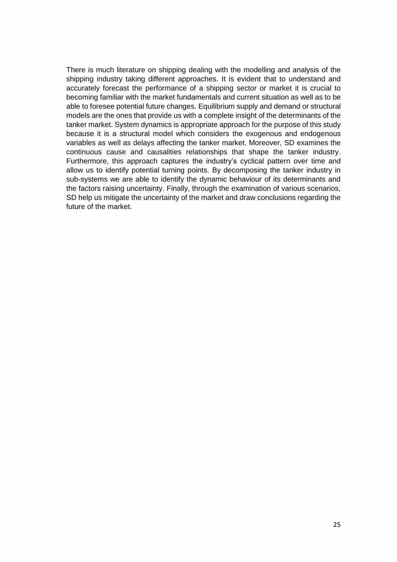
25

There is much literature on shipping dealing with the modelling and analysis of the

shipping industry taking different approaches. It is evident that to understand and

accurately forecast the performance of a shipping sector or market it is crucial to

becoming familiar with the market fundamentals and current situation as well as to be

able to foresee potential future changes. Equilibrium supply and demand or structural

models are the ones that provide us with a complete insight of the determinants of the

tanker market. System dynamics is appropriate approach for the purpose of this study

because it is a structural model which considers the exogenous and endogenous

variables as well as delays affecting the tanker market. Moreover, SD examines the

continuous cause and causalities relationships that shape the tanker industry.

Furthermore, this approach captures the industry’s cyclical pattern over time and

allow us to identify potential turning points. By decomposing the tanker industry in

sub-systems we are able to identify the dynamic behaviour of its determinants and

the factors raising uncertainty. Finally, through the examination of various scenarios,

SD help us mitigate the uncertainty of the market and draw conclusions regarding the

future of the market.

26

Chapter 6 Methodology and Data

6.1. Introduction

Chapters 1 to 5 aimed to provide an overview of the shipping market and its

mechanisms. After having gone through various academic papers and theories

explaining the shipping market theory, in Figure 6 below, we summarize the

mechanisms of the industry. In this chapter, we attempt to construct a simple system

dynamics model in order to forecast turning points in the crude oil tanker market in

the foreseeable future examining the capacity demanded and supplied. To achieve

our goal, we examine the balance between supply of and demand for tonnage as it is

the determinant of the freight rates.

Figure 6: The Mechanism of Shipping Source: Compiled by author via various sources (Zannetos 1966, Beenstock &

Vergottis 1989 and 1993)

Time charter rates reflect the expectations of shipowners regarding the spot market.

It is apparent in the figure above that newbuilding market is affected by the level of

time charter rates. In turn, the amount of new tonnage delivered coupled with the

tonnage scrapped affect the balance between supply and demand which affect the

voyage or spot charter rates.

It is obvious that voyage and time charters move together to the same direction

depending on the market balance. If there is oversupply, both voyage and time

charters decrease. Demand for shipping is equal to the tonnage demanded times the

average haul. On the other hand, supply for shipping equals to the tonnage supplied

multiplied by the fleet productivity. Both demand and supply are measured in tonne

miles and the balance between them form the freight rates. Since it is difficult to

estimate the average haul and the fleet productivity we concentrate on the capacity.

To achieve our goal, we built a capacity model for VLCC, Suezmax and Aframax

crude tankers for the years 2016-2035. We do not include Panamax tankers as these

vessels were involved only in the transportation of dirty petroleum products for the

year 2015.To build our system dynamics model we employ a computer simulation

model called Vensim PLE.

27

6.2. Variables Used in the Model

Our demand and supply tonnage model requires a set of variables. The future

demand for tonnage is affected by future oil trade and various random shocks.

Changes in the annual oil sea trade is a good indicator for the expected demand

growth. On the other hand, future random shocks are unpredictable and therefore,

difficult to be captured.

The tonnage supply is affected by changes in the active merchant fleet. The active

merchant fleet in the beginning of each year equals to the active merchant fleet in the

begging of the previous year plus the deliveries minus the scrapped and laid up

vessels of that year. The deliveries are based on the orders placed which are recorded

in the orderbook.

To conclude, the dependent variable we employ in our research for the assessment

of the crude market industry is the market equilibrium which reflects the balance

between the supply of and demand for tanker capacity. Therefore, our independent

variables are the supply of and demand for tanker tonnage.

Moreover, we employ a variable called forecast error which indicates the inability of

shipowners to balance demand and supply.

6.3. Data Collection and Structure

Data collection is a very time-consuming task which should be carried out carefully.

The quality of the data set gathered ensures the high performance of the system.

Reliable sources of data will ensure the validity of the data set and as a result, the

quality of our results. The main source we used in order to acquire our desired set of

data is the Clarksons Shipping Intelligence Network, provided by Clarksons, the most

respectable shipbroking firm in the world. Clarksons is widely known for the quality of

its shipping industry reports and has earned the respect of the shipping practitioners.

Our model requires annual data for a single year. The sample employed consists of

annual data of 2015. More specifically, we collected data for both the active merchant

fleet and orderbook at the end of 2015 in million DWT, for each category of crude

tanker involved in our study. Furthermore, regarding demand, we got the aggregate

demand in million DWT for each type of crude for the 2015. Furthermore, we collected

the seaborne trade in million tonnes from 2000-2015 so that we are able to come up

with an average growth which will constitute the main impact on the future demand.

A problem we encountered in the Clarksons database is that the VLCC category

contains both VLCC and ULCC vessels. This is the reason why we do not mention

ULCCs in the type of vessels we study as we consider them as one category.

28

6.4. Methodology

6.4.1. Introductory Comments and Assumptions

Shipping cycles are divided into the short and long cycles. In the short cycle, supply

is adjusted by changes in the vessels productivity, while in the long cycle, which last

20 years, by changes in the fleet capacity. Since we aim to build a capacity model,

we examine the market only in terms of capacity demanded and supplied. We want

to study the impact of the long cycle in the coming years. Therefore, we do not include

factors affecting the short cycles such as fleet productivity and costs of new vessels.

Also, we assume no vessels in lay-up as it is difficult to quantify them.

The S&P market is an auxiliary market and any activity in this market does not affect

our model since supply remains the same with the sale and purchase of a second-

hand vessel. Furthermore, we make the assumption that shipowners are willing to

scrap the fleet of twenty years old and above. Finally, we treat demand as an

exogenous factor and assume that no random shocks, which distort demand for oil

trade, will take place in the period of our study.

The crude tanker industry is a competitive one. Information regarding the market

conditions is freely available to all the existing or future investors. However, the

shipowners act irrationally and take decisions based on their expectations. Crude

tanker shipping companies offer homogeneous product and there is no impact on the

market by a single company or owner. Therefore, we build an aggregate model for

three sub-markets of the crude tanker market (VLCC, Suezmax, Aframax).

After having explained our assumptions and way of thinking, in the next two sections,

we present the dynamics of the crude tanker market as well as all the necessary

mathematical equations on which we construct our crude tanker capacity model.

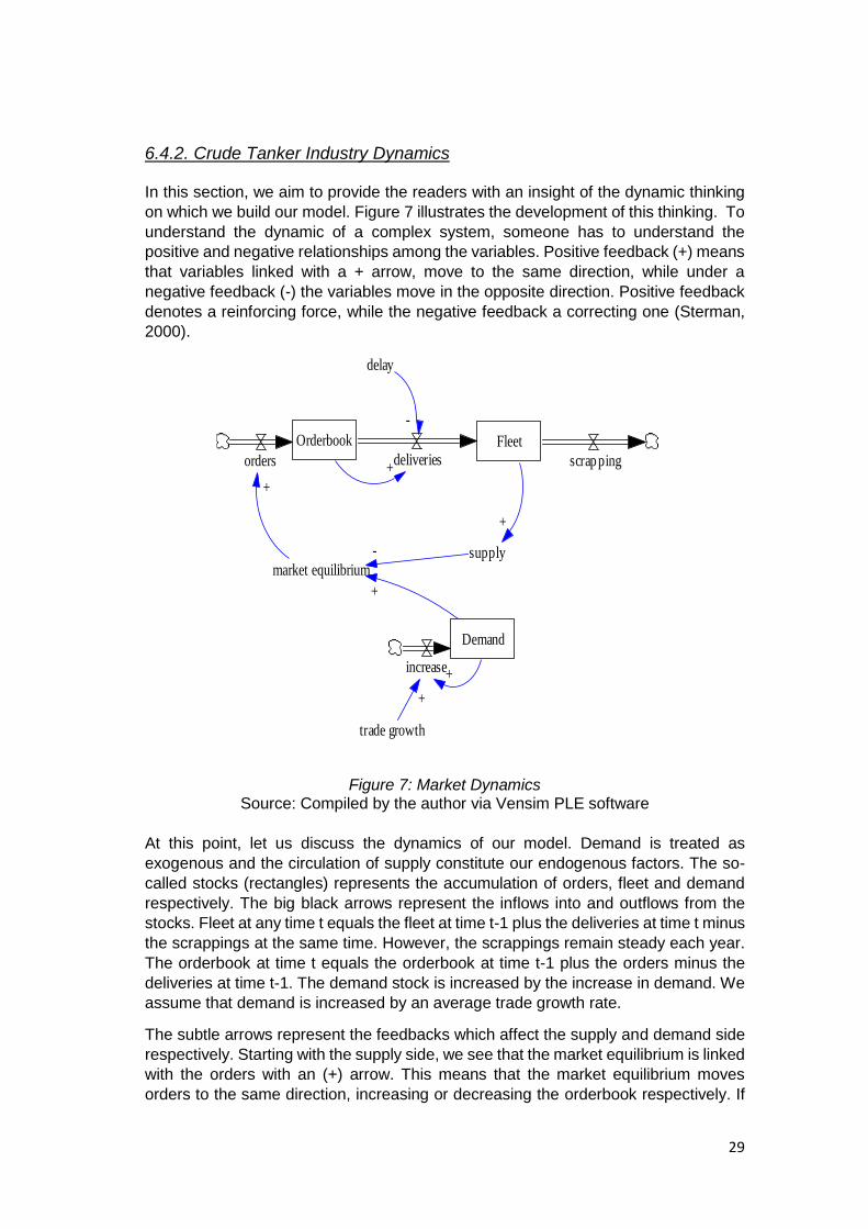
29

6.4.2. Crude Tanker Industry Dynamics

In this section, we aim to provide the readers with an insight of the dynamic thinking

on which we build our model. Figure 7 illustrates the development of this thinking. To

understand the dynamic of a complex system, someone has to understand the

positive and negative relationships among the variables. Positive feedback (+) means

that variables linked with a + arrow, move to the same direction, while under a

negative feedback (-) the variables move in the opposite direction. Positive feedback

denotes a reinforcing force, while the negative feedback a correcting one (Sterman,

2000).

Figure 7: Market Dynamics Source: Compiled by the author via Vensim PLE software

At this point, let us discuss the dynamics of our model. Demand is treated as

exogenous and the circulation of supply constitute our endogenous factors. The so-

called stocks (rectangles) represents the accumulation of orders, fleet and demand

respectively. The big black arrows represent the inflows into and outflows from the

stocks. Fleet at any time t equals the fleet at time t-1 plus the deliveries at time t minus

the scrappings at the same time. However, the scrappings remain steady each year.

The orderbook at time t equals the orderbook at time t-1 plus the orders minus the

deliveries at time t-1. The demand stock is increased by the increase in demand. We

assume that demand is increased by an average trade growth rate.

The subtle arrows represent the feedbacks which affect the supply and demand side

respectively. Starting with the supply side, we see that the market equilibrium is linked

with the orders with an (+) arrow. This means that the market equilibrium moves

orders to the same direction, increasing or decreasing the orderbook respectively. If

Orderbook Fleet

orders deliveries scrapping

supply

+

market equilibrium

-

+

Demand

increase

trade growth

+

+

+

delay

-

+

30

the market equilibrium increases, then orders increase and shipowners order vessels

to balance demand and supply. If the market equilibrium decreases, then orders fall.

In turn, orderbook is linked with the deliveries with a positive feedback (+). The more

the orderbook the more the deliveries. However, deliveries are affected exogenously

by the time of construction (delays). Since they are linked with a (-) arrow, they move

to the opposite direction. The more the delays, the less the deliveries at time t. Fleet

is affected by deliveries and scrappings. The more the deliveries the more the fleet,

while scrapping correct the market putting out of the market the old vessels. Supply

equals the active fleet at time t. Thus, fleet and supply moves to the same direction

and are linked with a positive feedback arrow. Supply is linked to the market

equilibrium with a negative feedback (-) as the more the ships available, the lower the

market equilibrium point.

Demand moves to the same direction with the market equilibrium. An increase in the

demand increases the market equilibrium as the difference between demand and

supply increases. Demand is determined by the demand of the year t-1 plus the

increase of the demand at time t, which in turn is affected the average trade growth.

Any relationship in the demand side is characterized by the positive feedbacks (+).

Any increase in the starting demand and trade average trade growth increase the

demand at time t.

6.4.3. Model Equations

In this section, we present the mathematical equations we use in our system dynamics

base model (Vensim Software Model)6. Each equation presented below is aggregate

for each type of tankers examined (VLCC, Suezmax, Aframax).

Kyra Schuit (2004), in her thesis, constructs a dynamic world tanker market capacity

model over a 20-year period. The purpose of her model is to identify the economic

structure as well as to study the factors causing cyclicality in the tanker market (Schuit,

2004). Considering three different initial market situations (balance, shortage,

overcapacity) she attempts to build a capacity model based on four different order

strategies. She considers market balance as the difference between the expected

demand at the delivery time of new vessels minus the current active fleet. In order to

identify supply in terms of demand, she multiplied active fleet by a fixed vessel

performance, while based on the balance condition she attempts to build the order

strategy. It is worth noting that according to her approach the final market situations

is independent of the initial one (Schuit, 2004).

In this section, we attempt to build a dynamic capacity model for three different types

of tankers in order to predict the crude tanker market in the foreseeable future. Our

modelling approach differs to that of Kyra Schuit both in terms of purpose and time

period. We consider both demand and supply in terms of DWT bypassing

performance since it does not display dynamic behaviour. Vessel performance is

determined by the haul of a specific trip (route) and the speed a vessel sails. However,

routes and sailing speeds are fixed over time. Moreover, we argue that ordering

strategy is based on the market balance at each time t defined by the balance

6 Appendix 1: Vensim Software Model

31

between demand and supply at that time. The model equations and assumptions used

in our model are discussed in the following paragraphs.

The crude tanker market is very dynamic and shipowners' daily decisions lead to

processes of continuous market adjustments. The number of orders placed as well

as the scrapped and laid up vessels constitute the endogenous factors that distort the

market. Changes in these variables influence the number of ships in the active fleet

and as a result, the capacity offered for crude oil transport by sea.

Our analysis will examine each type of crude tankers separately. The formulas of our

model are constructed to be applicable for each type of vessel we consider. The

active merchant fleet at the end of year t equals the merchant fleet of the past year

plus the deliveries minus the scrapped and laid up vessels during year t.

For simplicity, in our model we do not include vessels in lay-up and consider them as

part of the active fleet as these ships can enter the market at any time. Moreover, we

consider the vessels used for oil storage as part of the active fleet as the duration of

the contracts is not specified in our data set. Therefore, based on our assumptions,

the active fleet at time t equals the fleet at t-1 plus the deliveries minus the scrapping

activity during time t.

1 ,, , ,t j t j j t jtF F D S for t=1,2,….,N and j=1,2,3 (1)

Where:

t= time

j= the type of crude tanker for j=1 (VLCC), 2 (Suezmax), 3 (Aframax)

F=active crude tanker fleet in DWT

Dt,j= the deliveries in DWT

St,j= the scrapped tonnage in DWT

As we have already discussed in the section devoted to the newbuilding market (see

section 2.4.2.), the time lag between the ordering and delivery of a new vessel ranges

from one to two years. We set construction time (L) 1.5 years, which is the average

of the time lag between the ordering and delivery of new vessels. This means that

deliveries at time t equal the orders placed t-1.5 years.

, ,t j t L jD O for t=0,1,2,…,N (2)

Where: t LO equals to zero till t=L

The orderbook (Kt,j) is keeping a record of the orders and deliveries placed and

depicted as stock in Figure 7 which is found in the section 6.4.2. We assume that the

orderbook is based on the first in-first out (FIFO) discipline. The orders placed first are

delivered first with a delay of 1.5 years. Every time t the orderbook increases with the

32

orders and decreases with the deliveries at time t. The orders represent the inflows to

the orderbook, while the deliveries the outflows.

, 1, , ,t j t j t j t jK K O D for t=1,2,,…,N and j=1,2,3 (3)

The orderbook of 2015 shows that most of the vessels under construction will be

delivered between 2016 and 2017. Moreover, data shows that the expected delivery

of new tonnage includes also tonnage ordered before 2015. To overcome this

problem we update the orderbook at the start of 2016 (K0,j)7 and assume that all

tankers are ordered at the start of 2016 and delivered 1.5 years later.

0, 0,j jK O (4)

According to Sterman (2000), the deliveries (outflows) in such a structure are always

proportional to orderbook (stock). The orderbook at time t is assumed to be delivered

at a rate of Kt,j /L per year. Since the at time t=0 the orderbook equals the orders, the

amount of K0,j /L is delivered the first year. This means that deliveries at time t (Dt,j)

are equal to Kt-1,j /L.

1,

,

t j

t j

KD

L

for t=1,2,…,N (5)

Based on the analysis above, the orderbook at any time t is given by the formula:

, 1, ,

1( )t j t j t j

LK K O

L

for t=1,2,…,N (6)

The delivery rate K0,j/L would deplete the orderbook in 1.5 years if no orders are

placed during this period. However, since the orderbook falls, so does the rate of the

deliveries leading to a small delay of the 100% of new tonnage. Both the orderbook

and deliveries follow an exponential decay pattern (Sterman, 2000). Upon this

approach, the greater the orderbook the greater the deliveries and thus, the rate of

decrease in the orderbook (Sterman, 2000).

We assume that shipowners are behaving irrationally during the time horizon of our

study. This means that they act based on the current market situation without

considering what will be the future conditions. Since they cannot predict the future

demand and its shocks, shipowners order according to the current market situation at

any time. Their ordering strategy depends on their expectations regarding the future

condition in the market. If there is a shortage or balance of tonnage at a time t

shipowners expect higher freight rates and therefore, order vessels. However, this

strategy leads to over-ordering (c) as the owners act based on the current situation

taking no into account future deliveries which increase the capacity of the fleet. We

consider this strategy in our model as we think it is as close as possible to the reality.

Moreover, we consider no shipbuilding costs. If demand is greater than or equal to

7 Appendix 3: Initial Orderbook 2016 in Million DWT

33

supply, then balance (Bt,j ) is not negative and shipowners order the necessary DWT

according to their expectations. In any other case, there are few aggressive

shipowners who place a limited number of orders causing overordering as well. The

balance of the market (Bt,j ) is discussed later in this section.

We assume that when the market balance is positive shipowners order 4% (r)

tonnage in excess.

IF , 0t jB then

, ,t j t jO cB , where c=1+r for t=0,1,2,…,N (7)

The supply meet demand instantaneously, because of the continuous adjustments

occurring in the market and the inability of the shipowners to balance demand and

supply. Therefore, we do not consider the case Bt,j=0.

If the market balance is negative, we assume that owners place orders equal to 0.5%

(q) of the market balance.

IF , 0t jB then

, ,t j t jO qB for t=0,1,2,…,N (8)

Our data shows that the crude tanker fleet, for each category, at the start of 2016 F(0,j)

is very modern. More specifically, 61.48% of the VLCC fleet, 63.80% of the Suezmax

and 57.80% of the Aframax is 10 years old. Shipowners are willing to scrap vessels

of 20 years old and above. We assume that expected freight rates will not affect the

scrapping activity further and the vessels are scrapped when they become 20 years

old. Therefore, the current order book should be scrapped in twenty years from now.

To acquire as realistic results as possible, we calculate the average number of DWT

that has to be scrapped8 per year and category of tankers based on our assumptions.

Thus, we derive a steady amount of scrapping in million DWT per year for each type

of tanker:

For j=1, 1 10.02S million DWT/year

For j=2, 2 3.76S million DWT/year

For j=3, 3 3.4S million DWT/year

The demand for seaborne oil transportation is considered completely inelastic and

treated as exogenous. It is obvious that the more the need for oil sea trade transport,

the more the demand for tankers. Therefore, we set expected demand in DWT (DDt,j)9

as linear function with the average annual percentage of oil sea trade growth (g)10:

8 Appendix 4: Annual Scraping rate Calculations in Million DWT

9 Appendix 5: Initial Demand 2016 in Million DWT

10 Appendix 6: Average Annual Trade Growth in Million Tonnes

34

, 0(1 )t jDD DD gt for t=1,2,…,N (9)

The balance between demand and supply shows the market situation in terms of

capacity demanded and offered. If the difference between demand and supply is zero,

then the market is in balance. If demand greater than supply, then there is a tanker

shortage capacity followed by an increase in freights. Finally, if the difference is

negative, there is overcapacity of tankers which in turn suppress the charter rates.

, , ,t j t j t jB DD F for t=0,1,…,N (10)

Shipowners fail to forecast the future market situation causing market distortion

arising from their ordering strategy. We employ a forecast error indicator (Rt,j) which

indicates the divergence between shipowners expectations at time t about the actual

market situation at time t+L, where deliveries are placed.Forecast error indicator (Rt,j)

at any time t is equal to the fleet at time t plus the orderbook at time t minus the sum

of scrappings during the period t+l minus the demand at time t+L when the orders at

time t are delivered. The following analysis shows the impact of the order strategy on

future market balance at time t+L.

, , , , ,t j t j t j t j t L jR F K LS DD , for t=0,1…, N (11)

, where (1 )t L tDD DD gL and g=the annual oil seaborne trade growth

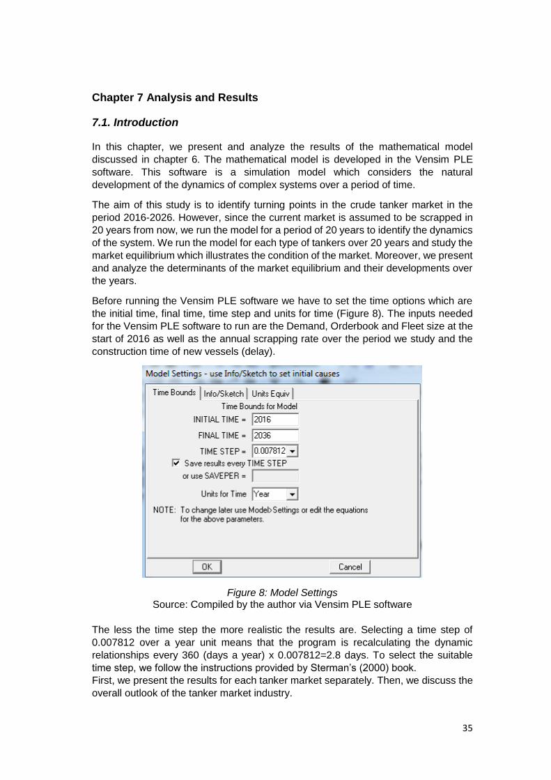
35

Chapter 7 Analysis and Results

7.1. Introduction

In this chapter, we present and analyze the results of the mathematical model

discussed in chapter 6. The mathematical model is developed in the Vensim PLE

software. This software is a simulation model which considers the natural

development of the dynamics of complex systems over a period of time.

The aim of this study is to identify turning points in the crude tanker market in the

period 2016-2026. However, since the current market is assumed to be scrapped in

20 years from now, we run the model for a period of 20 years to identify the dynamics

of the system. We run the model for each type of tankers over 20 years and study the

market equilibrium which illustrates the condition of the market. Moreover, we present

and analyze the determinants of the market equilibrium and their developments over

the years.

Before running the Vensim PLE software we have to set the time options which are

the initial time, final time, time step and units for time (Figure 8). The inputs needed

for the Vensim PLE software to run are the Demand, Orderbook and Fleet size at the

start of 2016 as well as the annual scrapping rate over the period we study and the

construction time of new vessels (delay).

Figure 8: Model Settings Source: Compiled by the author via Vensim PLE software

The less the time step the more realistic the results are. Selecting a time step of

0.007812 over a year unit means that the program is recalculating the dynamic

relationships every 360 (days a year) x 0.007812=2.8 days. To select the suitable

time step, we follow the instructions provided by Sterman’s (2000) book.

First, we present the results for each tanker market separately. Then, we discuss the

overall outlook of the tanker market industry.

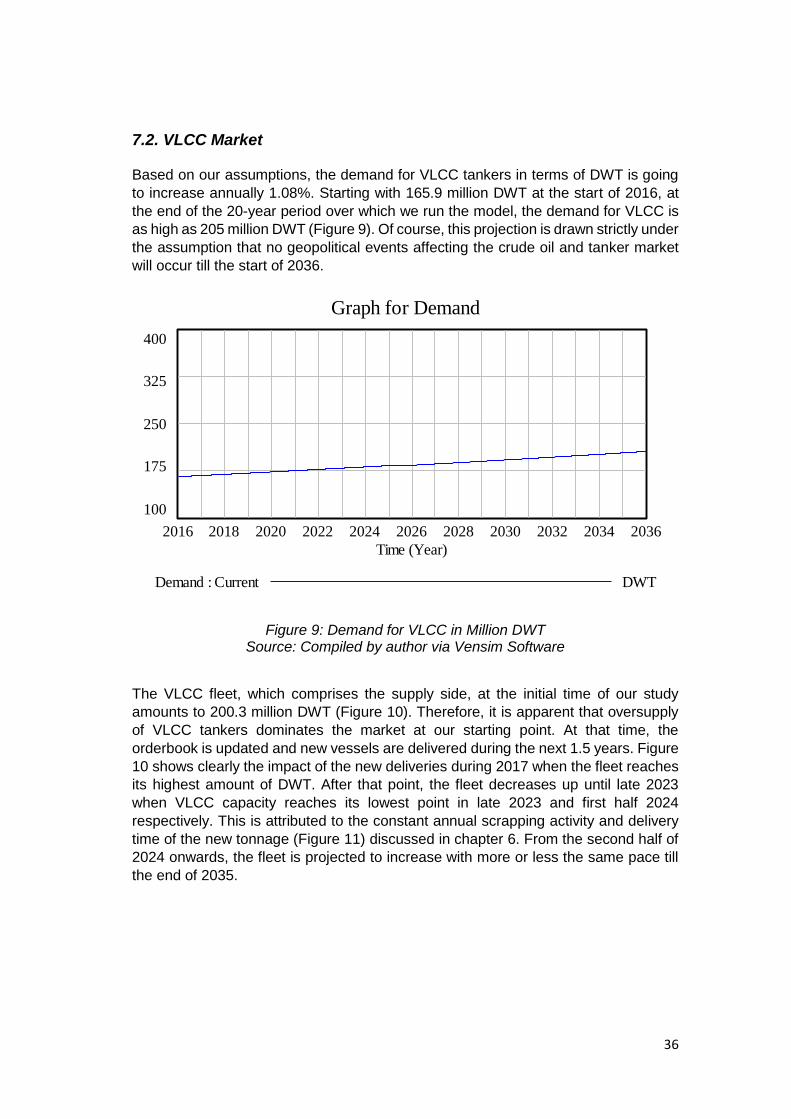
36

7.2. VLCC Market

Based on our assumptions, the demand for VLCC tankers in terms of DWT is going

to increase annually 1.08%. Starting with 165.9 million DWT at the start of 2016, at

the end of the 20-year period over which we run the model, the demand for VLCC is

as high as 205 million DWT (Figure 9). Of course, this projection is drawn strictly under

the assumption that no geopolitical events affecting the crude oil and tanker market

will occur till the start of 2036.

Figure 9: Demand for VLCC in Million DWT Source: Compiled by author via Vensim Software

The VLCC fleet, which comprises the supply side, at the initial time of our study

amounts to 200.3 million DWT (Figure 10). Therefore, it is apparent that oversupply

of VLCC tankers dominates the market at our starting point. At that time, the

orderbook is updated and new vessels are delivered during the next 1.5 years. Figure

10 shows clearly the impact of the new deliveries during 2017 when the fleet reaches

its highest amount of DWT. After that point, the fleet decreases up until late 2023

when VLCC capacity reaches its lowest point in late 2023 and first half 2024

respectively. This is attributed to the constant annual scrapping activity and delivery

time of the new tonnage (Figure 11) discussed in chapter 6. From the second half of

2024 onwards, the fleet is projected to increase with more or less the same pace till

the end of 2035.

Graph for Demand

400

325

250

175

100

2016 2018 2020 2022 2024 2026 2028 2030 2032 2034 2036

Time (Year)

Demand : Current DWT

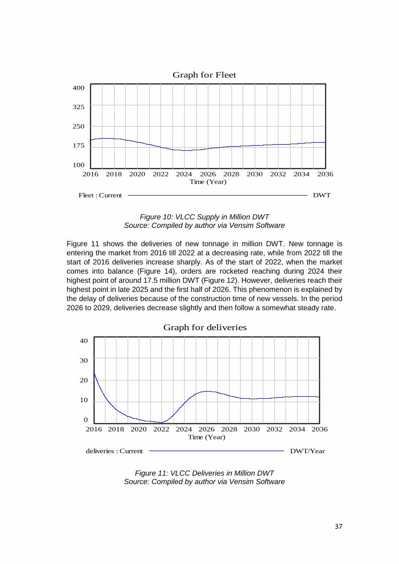
37

Figure 10: VLCC Supply in Million DWT Source: Compiled by author via Vensim Software

Figure 11 shows the deliveries of new tonnage in million DWT. New tonnage is

entering the market from 2016 till 2022 at a decreasing rate, while from 2022 till the

start of 2016 deliveries increase sharply. As of the start of 2022, when the market

comes into balance (Figure 14), orders are rocketed reaching during 2024 their

highest point of around 17.5 million DWT (Figure 12). However, deliveries reach their

highest point in late 2025 and the first half of 2026. This phenomenon is explained by

the delay of deliveries because of the construction time of new vessels. In the period

2026 to 2029, deliveries decrease slightly and then follow a somewhat steady rate.

Figure 11: VLCC Deliveries in Million DWT Source: Compiled by author via Vensim Software

Graph for Fleet

400

325

250

175

100

2016 2018 2020 2022 2024 2026 2028 2030 2032 2034 2036

Time (Year)

Fleet : Current DWT

Graph for deliveries

40

30

20

10

0

2016 2018 2020 2022 2024 2026 2028 2030 2032 2034 2036

Time (Year)

deliveries : Current DWT/Year

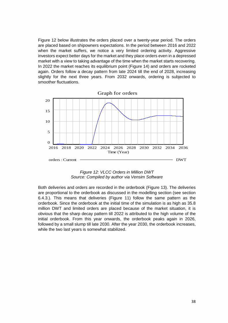
38

Figure 12 below illustrates the orders placed over a twenty-year period. The orders

are placed based on shipowners expectations. In the period between 2016 and 2022

when the market suffers, we notice a very limited ordering activity. Aggressive

investors expect better days for the market and they place orders even in a depressed

market with a view to taking advantage of the time when the market starts recovering.

In 2022 the market reaches its equilibrium point (Figure 14) and orders are rocketed

again. Orders follow a decay pattern from late 2024 till the end of 2028, increasing

slightly for the next three years. From 2032 onwards, ordering is subjected to

smoother fluctuations.

Figure 12: VLCC Orders in Million DWT Source: Compiled by author via Vensim Software

Both deliveries and orders are recorded in the orderbook (Figure 13). The deliveries

are proportional to the orderbook as discussed in the modelling section (see section

6.4.3.). This means that deliveries (Figure 11) follow the same pattern as the

orderbook. Since the orderbook at the initial time of the simulation is as high as 35.8

million DWT and limited orders are placed because of the market situation, it is

obvious that the sharp decay pattern till 2022 is attributed to the high volume of the

initial orderbook. From this year onwards, the orderbook peaks again in 2026,

followed by a small slump till late 2030. After the year 2030, the orderbook increases,

while the two last years is somewhat stabilized.

Graph for orders

20

15

10

5

0

2016 2018 2020 2022 2024 2026 2028 2030 2032 2034 2036

Time (Year)

orders : Current DWT

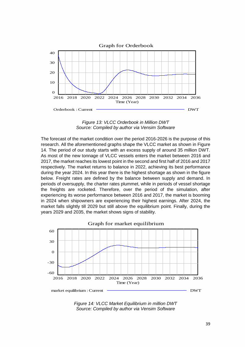
39

Figure 13: VLCC Orderbook in Million DWT Source: Compiled by author via Vensim Software

The forecast of the market condition over the period 2016-2026 is the purpose of this

research. All the aforementioned graphs shape the VLCC market as shown in Figure

14. The period of our study starts with an excess supply of around 35 million DWT.

As most of the new tonnage of VLCC vessels enters the market between 2016 and

2017, the market reaches its lowest point in the second and first half of 2016 and 2017

respectively. The market returns to balance in 2022, achieving its best performance

during the year 2024. In this year there is the highest shortage as shown in the figure

below. Freight rates are defined by the balance between supply and demand. In

periods of oversupply, the charter rates plummet, while in periods of vessel shortage

the freights are rocketed. Therefore, over the period of the simulation, after

experiencing its worse performance between 2016 and 2017, the market is booming

in 2024 when shipowners are experiencing their highest earnings. After 2024, the

market falls slightly till 2029 but still above the equilibrium point. Finally, during the

years 2029 and 2035, the market shows signs of stability.

Figure 14: VLCC Market Equilibrium in million DWT Source: Compiled by author via Vensim Software

Graph for Orderbook

40

30

20

10

0

2016 2018 2020 2022 2024 2026 2028 2030 2032 2034 2036

Time (Year)

Orderbook : Current DWT

Graph for market equilibrium

60

30

0

-30

-60

2016 2018 2020 2022 2024 2026 2028 2030 2032 2034 2036

Time (Year)

market equilibrium : Current DWT

40

Figure 15 shows the shipowners’ forecast error, which in essence reflects the

divergence between their decisions, which are based on their expectations about

future VLCC market condition, and the actual future market situation. The graph

shows that the forecast error is very high in times of oversupply, while when the

market rebounds is becoming lower. The graph shows the inability of the owners to

balance supply and demand. It is worth noticing that even when the market becomes

more stable (2028-2036), as observed in the figure above, the error still exists. As the

market rebounds and becomes more stable, the forecast error tends to disappear but

not completely. Therefore, it is obvious that the main determinant of the future VLCC

market situation is the decisions made by owners.

Figure 15: VLCC Shipowners Forecast Error in Million DWT Source: Compiled by author via Vensim Software

Graph for Forecast error

60

30

0

-30

-60

2016 2018 2020 2022 2024 2026 2028 2030 2032 2034 2036

Time (Year)

Forecast error : Current DWT

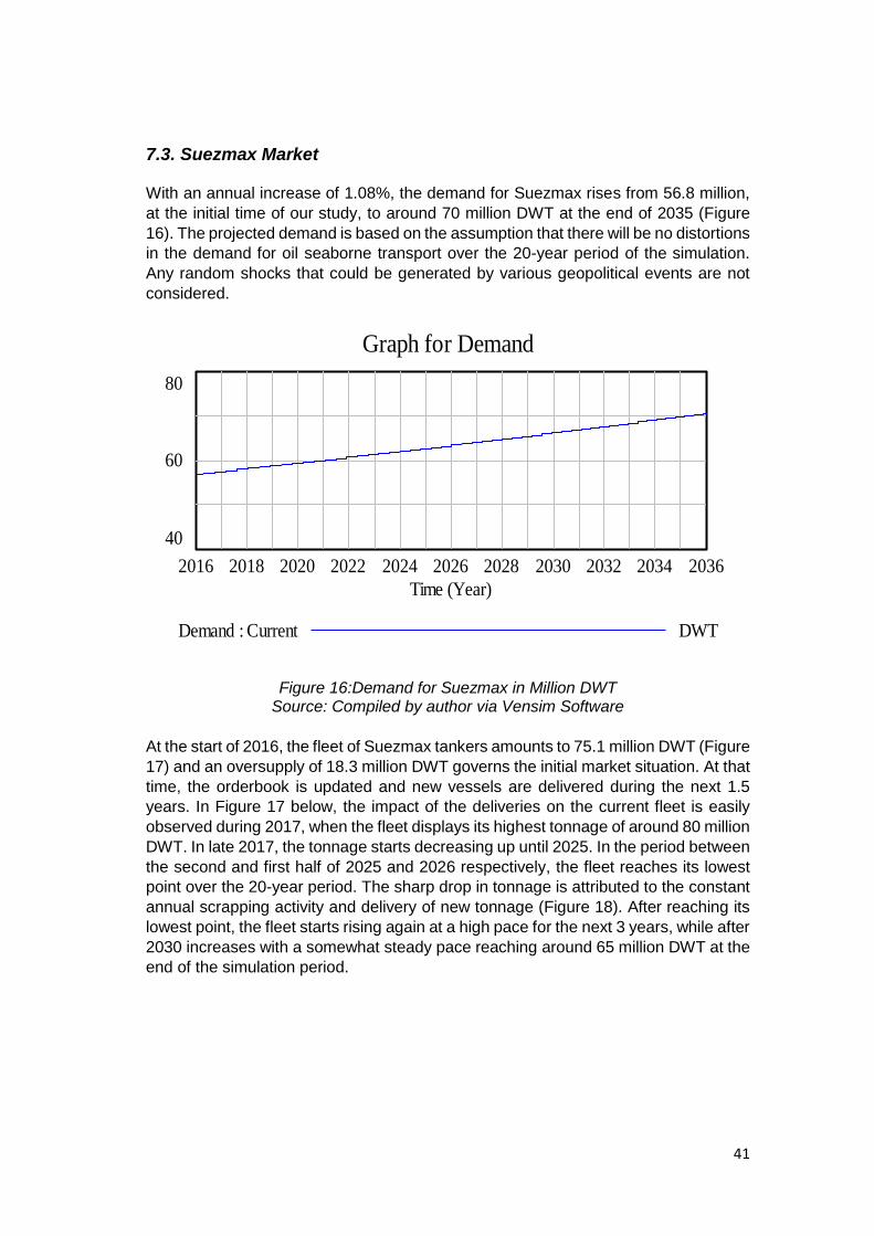
41

7.3. Suezmax Market

With an annual increase of 1.08%, the demand for Suezmax rises from 56.8 million,

at the initial time of our study, to around 70 million DWT at the end of 2035 (Figure

16). The projected demand is based on the assumption that there will be no distortions

in the demand for oil seaborne transport over the 20-year period of the simulation.

Any random shocks that could be generated by various geopolitical events are not

considered.

Figure 16:Demand for Suezmax in Million DWT Source: Compiled by author via Vensim Software

At the start of 2016, the fleet of Suezmax tankers amounts to 75.1 million DWT (Figure

17) and an oversupply of 18.3 million DWT governs the initial market situation. At that

time, the orderbook is updated and new vessels are delivered during the next 1.5

years. In Figure 17 below, the impact of the deliveries on the current fleet is easily

observed during 2017, when the fleet displays its highest tonnage of around 80 million

DWT. In late 2017, the tonnage starts decreasing up until 2025. In the period between

the second and first half of 2025 and 2026 respectively, the fleet reaches its lowest

point over the 20-year period. The sharp drop in tonnage is attributed to the constant

annual scrapping activity and delivery of new tonnage (Figure 18). After reaching its

lowest point, the fleet starts rising again at a high pace for the next 3 years, while after

2030 increases with a somewhat steady pace reaching around 65 million DWT at the

end of the simulation period.

Graph for Demand

80

60

40

2016 2018 2020 2022 2024 2026 2028 2030 2032 2034 2036

Time (Year)

Demand : Current DWT

42

Figure 17:Suezmax Supply in Million DWT Source: Compiled by author via Vensim Software

The deliveries of new tonnage in million DWT are illustrated in Figure 18. New

tonnage flows into the market at a decreasing rate between 2016 and 2023, while

from 2024 onwards, deliveries are rocketed again till 2028. Since late 2023, when the

market returns to balance (Figure 21), orders are rocketed reaching in 2026 their

highest point of something less than 7 million DWT (Figure 19). Deliveries reach their

highest amount of tonnage in the second and first half of 2027 and 2028 respectively.

The delay between ordering and delivery is explained by the construction time of new

vessels. Between 2028 and 2032 deliveries decrease slightly and then they follow a

somewhat steady rate.

Figure 18:Suezmax Deliveries in Million DWT Source: Compiled by author via Vensim Software

Graph for Fleet

80

70

60

50

40

2016 2018 2020 2022 2024 2026 2028 2030 2032 2034 2036

Time (Year)

Fleet : Current DWT

Graph for deliveries

20

15

10

5

0

2016 2018 2020 2022 2024 2026 2028 2030 2032 2034 2036

Time (Year)

deliveries : Current DWT/Year

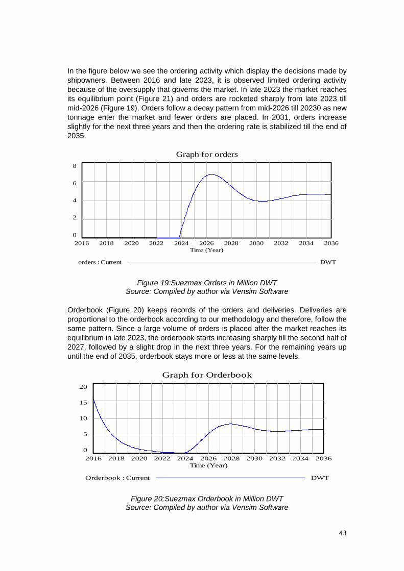
43

In the figure below we see the ordering activity which display the decisions made by

shipowners. Between 2016 and late 2023, it is observed limited ordering activity

because of the oversupply that governs the market. In late 2023 the market reaches

its equilibrium point (Figure 21) and orders are rocketed sharply from late 2023 till

mid-2026 (Figure 19). Orders follow a decay pattern from mid-2026 till 20230 as new

tonnage enter the market and fewer orders are placed. In 2031, orders increase

slightly for the next three years and then the ordering rate is stabilized till the end of

2035.

Figure 19:Suezmax Orders in Million DWT Source: Compiled by author via Vensim Software

Orderbook (Figure 20) keeps records of the orders and deliveries. Deliveries are

proportional to the orderbook according to our methodology and therefore, follow the

same pattern. Since a large volume of orders is placed after the market reaches its

equilibrium in late 2023, the orderbook starts increasing sharply till the second half of

2027, followed by a slight drop in the next three years. For the remaining years up

until the end of 2035, orderbook stays more or less at the same levels.

Figure 20:Suezmax Orderbook in Million DWT Source: Compiled by author via Vensim Software

Graph for orders

8

6

4

2

0

2016 2018 2020 2022 2024 2026 2028 2030 2032 2034 2036

Time (Year)

orders : Current DWT

Graph for Orderbook

20

15

10

5

0

2016 2018 2020 2022 2024 2026 2028 2030 2032 2034 2036

Time (Year)

Orderbook : Current DWT

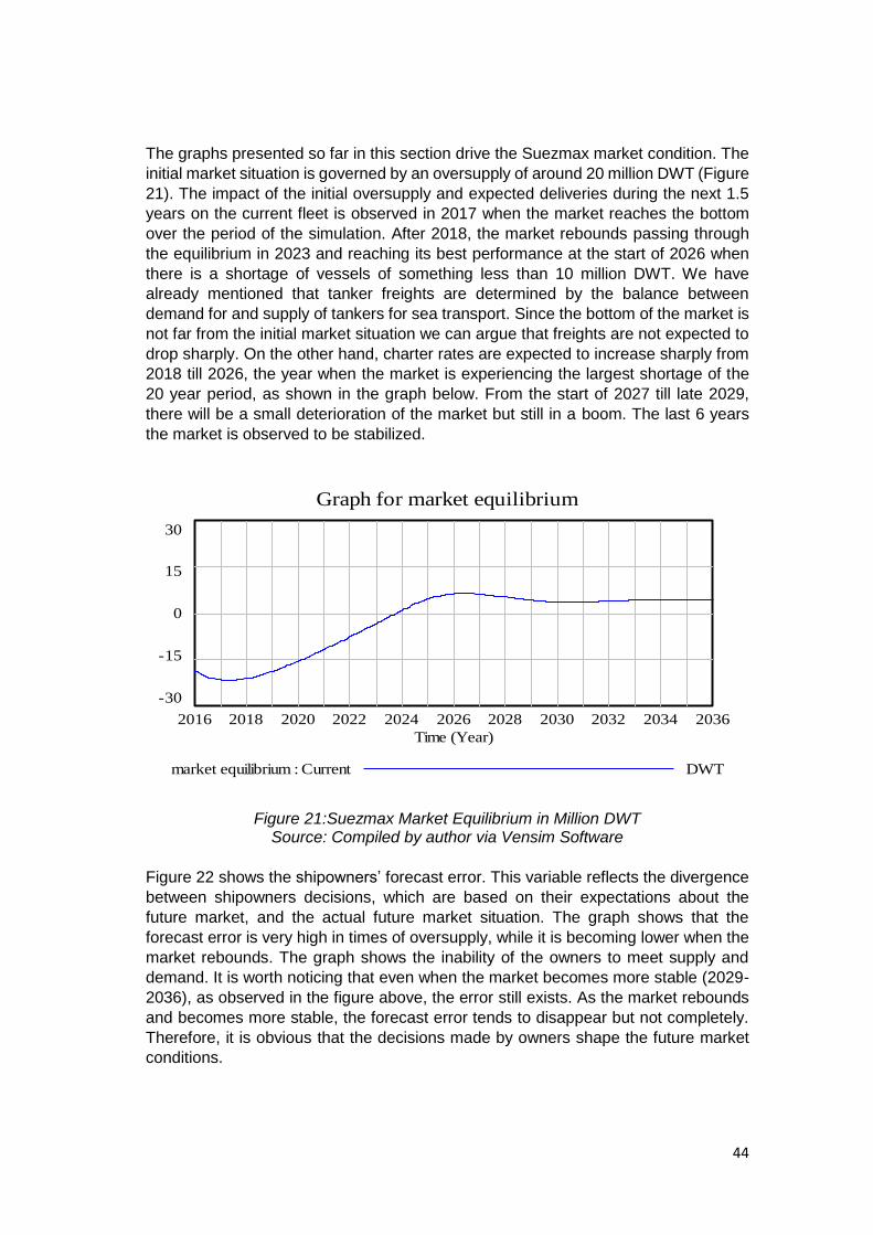
44

The graphs presented so far in this section drive the Suezmax market condition. The

initial market situation is governed by an oversupply of around 20 million DWT (Figure

21). The impact of the initial oversupply and expected deliveries during the next 1.5

years on the current fleet is observed in 2017 when the market reaches the bottom

over the period of the simulation. After 2018, the market rebounds passing through

the equilibrium in 2023 and reaching its best performance at the start of 2026 when

there is a shortage of vessels of something less than 10 million DWT. We have

already mentioned that tanker freights are determined by the balance between

demand for and supply of tankers for sea transport. Since the bottom of the market is

not far from the initial market situation we can argue that freights are not expected to

drop sharply. On the other hand, charter rates are expected to increase sharply from

2018 till 2026, the year when the market is experiencing the largest shortage of the

20 year period, as shown in the graph below. From the start of 2027 till late 2029,

there will be a small deterioration of the market but still in a boom. The last 6 years

the market is observed to be stabilized.

Figure 21:Suezmax Market Equilibrium in Million DWT Source: Compiled by author via Vensim Software

Figure 22 shows the shipowners’ forecast error. This variable reflects the divergence

between shipowners decisions, which are based on their expectations about the

future market, and the actual future market situation. The graph shows that the

forecast error is very high in times of oversupply, while it is becoming lower when the

market rebounds. The graph shows the inability of the owners to meet supply and

demand. It is worth noticing that even when the market becomes more stable (2029-

2036), as observed in the figure above, the error still exists. As the market rebounds

and becomes more stable, the forecast error tends to disappear but not completely.

Therefore, it is obvious that the decisions made by owners shape the future market

conditions.

Graph for market equilibrium

30

15

0

-15

-30

2016 2018 2020 2022 2024 2026 2028 2030 2032 2034 2036

Time (Year)

market equilibrium : Current DWT

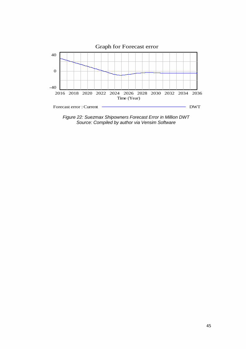
45

Figure 22: Suezmax Shipowners Forecast Error in Million DWT

Source: Compiled by author via Vensim Software

Graph for Forecast error

40

0

-40

2016 2018 2020 2022 2024 2026 2028 2030 2032 2034 2036

Time (Year)

Forecast error : Current DWT

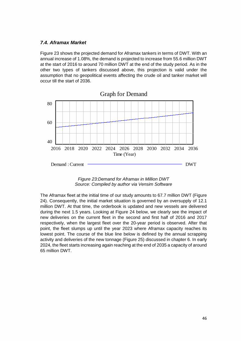
46

7.4. Aframax Market

Figure 23 shows the projected demand for Aframax tankers in terms of DWT. With an

annual increase of 1.08%, the demand is projected to increase from 55.6 million DWT

at the start of 2016 to around 70 million DWT at the end of the study period. As in the

other two types of tankers discussed above, this projection is valid under the

assumption that no geopolitical events affecting the crude oil and tanker market will

occur till the start of 2036.

Figure 23:Demand for Aframax in Million DWT Source: Compiled by author via Vensim Software

The Aframax fleet at the initial time of our study amounts to 67.7 million DWT (Figure

24). Consequently, the initial market situation is governed by an oversupply of 12.1

million DWT. At that time, the orderbook is updated and new vessels are delivered

during the next 1.5 years. Looking at Figure 24 below, we clearly see the impact of

new deliveries on the current fleet in the second and first half of 2016 and 2017

respectively, when the largest fleet over the 20-year period is observed. After that

point, the fleet slumps up until the year 2023 where Aframax capacity reaches its

lowest point. The course of the blue line below is defined by the annual scrapping

activity and deliveries of the new tonnage (Figure 25) discussed in chapter 6. In early

2024, the fleet starts increasing again reaching at the end of 2035 a capacity of around

65 million DWT.

Graph for Demand

80

60

40

2016 2018 2020 2022 2024 2026 2028 2030 2032 2034 2036

Time (Year)

Demand : Current DWT

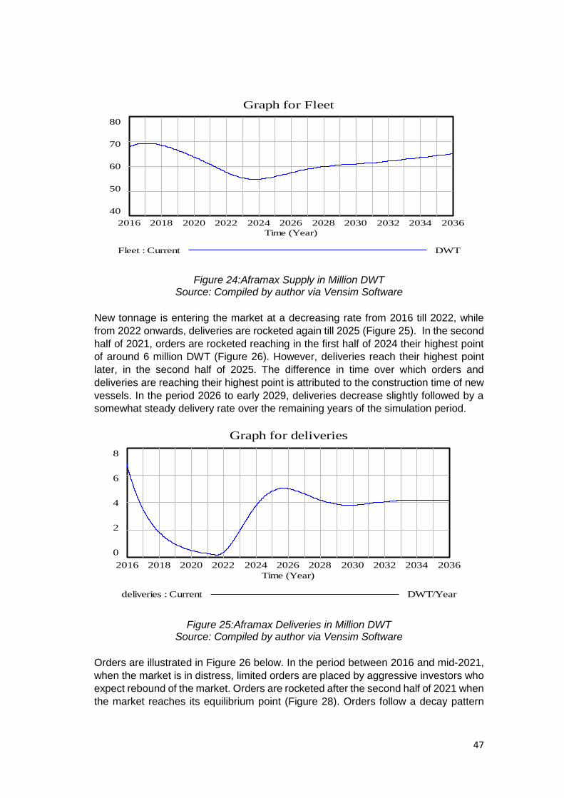
47

Figure 24:Aframax Supply in Million DWT Source: Compiled by author via Vensim Software

New tonnage is entering the market at a decreasing rate from 2016 till 2022, while

from 2022 onwards, deliveries are rocketed again till 2025 (Figure 25). In the second

half of 2021, orders are rocketed reaching in the first half of 2024 their highest point

of around 6 million DWT (Figure 26). However, deliveries reach their highest point

later, in the second half of 2025. The difference in time over which orders and

deliveries are reaching their highest point is attributed to the construction time of new

vessels. In the period 2026 to early 2029, deliveries decrease slightly followed by a

somewhat steady delivery rate over the remaining years of the simulation period.

Figure 25:Aframax Deliveries in Million DWT Source: Compiled by author via Vensim Software

Orders are illustrated in Figure 26 below. In the period between 2016 and mid-2021,

when the market is in distress, limited orders are placed by aggressive investors who

expect rebound of the market. Orders are rocketed after the second half of 2021 when

the market reaches its equilibrium point (Figure 28). Orders follow a decay pattern

Graph for Fleet

80

70

60

50

40

2016 2018 2020 2022 2024 2026 2028 2030 2032 2034 2036

Time (Year)

Fleet : Current DWT

Graph for deliveries

8

6

4

2

0

2016 2018 2020 2022 2024 2026 2028 2030 2032 2034 2036

Time (Year)

deliveries : Current DWT/Year

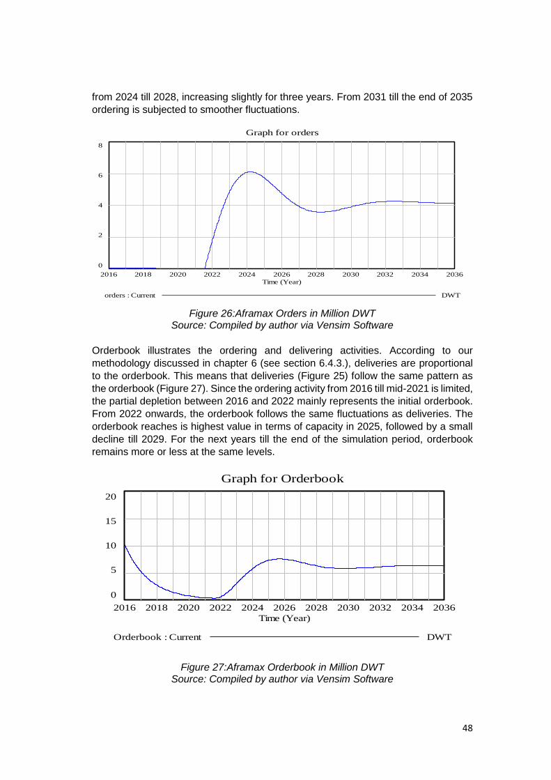
48

from 2024 till 2028, increasing slightly for three years. From 2031 till the end of 2035

ordering is subjected to smoother fluctuations.

Figure 26:Aframax Orders in Million DWT

Source: Compiled by author via Vensim Software

Orderbook illustrates the ordering and delivering activities. According to our

methodology discussed in chapter 6 (see section 6.4.3.), deliveries are proportional

to the orderbook. This means that deliveries (Figure 25) follow the same pattern as

the orderbook (Figure 27). Since the ordering activity from 2016 till mid-2021 is limited,

the partial depletion between 2016 and 2022 mainly represents the initial orderbook.

From 2022 onwards, the orderbook follows the same fluctuations as deliveries. The

orderbook reaches is highest value in terms of capacity in 2025, followed by a small

decline till 2029. For the next years till the end of the simulation period, orderbook

remains more or less at the same levels.

Figure 27:Aframax Orderbook in Million DWT Source: Compiled by author via Vensim Software

Graph for orders

8

6

4

2

0

2016 2018 2020 2022 2024 2026 2028 2030 2032 2034 2036

Time (Year)

orders : Current DWT

Graph for Orderbook

20

15

10

5

0

2016 2018 2020 2022 2024 2026 2028 2030 2032 2034 2036

Time (Year)

Orderbook : Current DWT

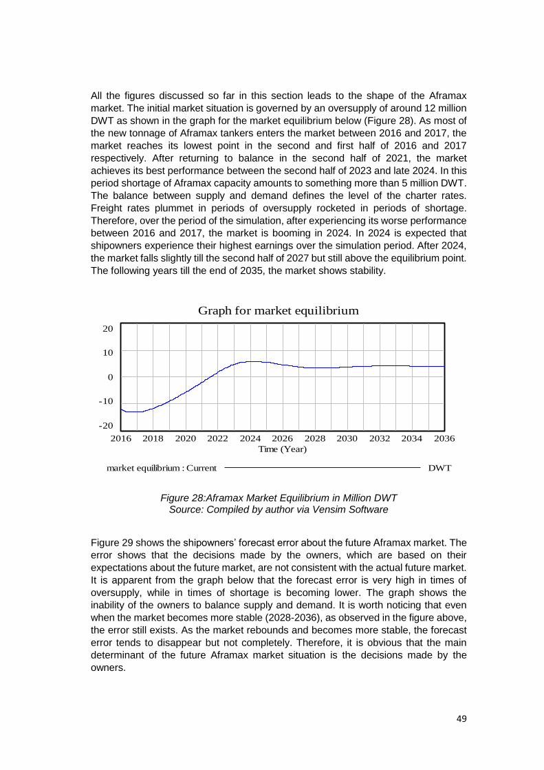
49

All the figures discussed so far in this section leads to the shape of the Aframax

market. The initial market situation is governed by an oversupply of around 12 million

DWT as shown in the graph for the market equilibrium below (Figure 28). As most of

the new tonnage of Aframax tankers enters the market between 2016 and 2017, the

market reaches its lowest point in the second and first half of 2016 and 2017

respectively. After returning to balance in the second half of 2021, the market

achieves its best performance between the second half of 2023 and late 2024. In this

period shortage of Aframax capacity amounts to something more than 5 million DWT.

The balance between supply and demand defines the level of the charter rates.

Freight rates plummet in periods of oversupply rocketed in periods of shortage.

Therefore, over the period of the simulation, after experiencing its worse performance

between 2016 and 2017, the market is booming in 2024. In 2024 is expected that

shipowners experience their highest earnings over the simulation period. After 2024,

the market falls slightly till the second half of 2027 but still above the equilibrium point.

The following years till the end of 2035, the market shows stability.

Figure 28:Aframax Market Equilibrium in Million DWT Source: Compiled by author via Vensim Software

Figure 29 shows the shipowners’ forecast error about the future Aframax market. The

error shows that the decisions made by the owners, which are based on their

expectations about the future market, are not consistent with the actual future market.

It is apparent from the graph below that the forecast error is very high in times of

oversupply, while in times of shortage is becoming lower. The graph shows the

inability of the owners to balance supply and demand. It is worth noticing that even

when the market becomes more stable (2028-2036), as observed in the figure above,

the error still exists. As the market rebounds and becomes more stable, the forecast

error tends to disappear but not completely. Therefore, it is obvious that the main

determinant of the future Aframax market situation is the decisions made by the

owners.

Graph for market equilibrium

20

10

0

-10

-20

2016 2018 2020 2022 2024 2026 2028 2030 2032 2034 2036

Time (Year)

market equilibrium : Current DWT

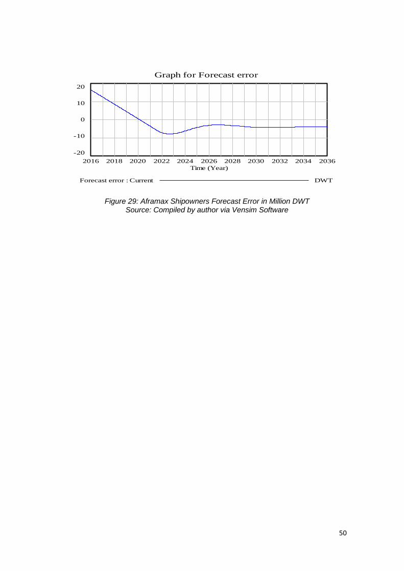
50

Figure 29: Aframax Shipowners Forecast Error in Million DWT Source: Compiled by author via Vensim Software

Graph for Forecast error

20

10

0

-10

-20

2016 2018 2020 2022 2024 2026 2028 2030 2032 2034 2036

Time (Year)

Forecast error : Current DWT

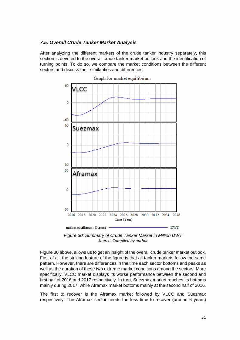
51

7.5. Overall Crude Tanker Market Analysis

After analyzing the different markets of the crude tanker industry separately, this

section is devoted to the overall crude tanker market outlook and the identification of

turning points. To do so, we compare the market conditions between the different

sectors and discuss their similarities and differences.

Figure 30: Summary of Crude Tanker Market in Million DWT Source: Compiled by author

Figure 30 above, allows us to get an insight of the overall crude tanker market outlook.

First of all, the striking feature of the figure is that all tanker markets follow the same

pattern. However, there are differences in the time each sector bottoms and peaks as

well as the duration of these two extreme market conditions among the sectors. More

specifically, VLCC market displays its worse performance between the second and

first half of 2016 and 2017 respectively. In turn, Suezmax market reaches its bottoms

mainly during 2017, while Aframax market bottoms mainly at the second half of 2016.

The first to recover is the Aframax market followed by VLCC and Suezmax

respectively. The Aframax sector needs the less time to recover (around 6 years)

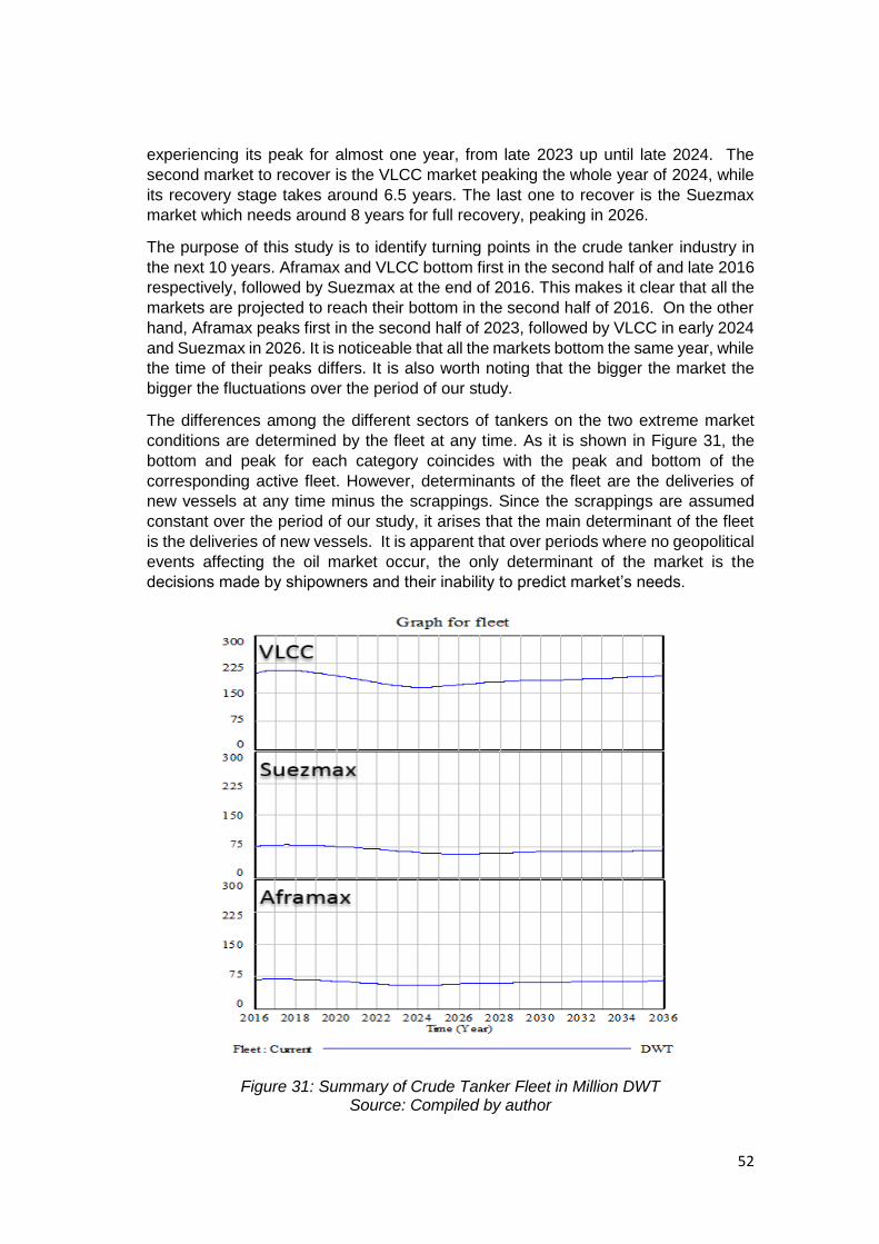
52

experiencing its peak for almost one year, from late 2023 up until late 2024. The

second market to recover is the VLCC market peaking the whole year of 2024, while

its recovery stage takes around 6.5 years. The last one to recover is the Suezmax

market which needs around 8 years for full recovery, peaking in 2026.

The purpose of this study is to identify turning points in the crude tanker industry in

the next 10 years. Aframax and VLCC bottom first in the second half of and late 2016

respectively, followed by Suezmax at the end of 2016. This makes it clear that all the

markets are projected to reach their bottom in the second half of 2016. On the other

hand, Aframax peaks first in the second half of 2023, followed by VLCC in early 2024

and Suezmax in 2026. It is noticeable that all the markets bottom the same year, while

the time of their peaks differs. It is also worth noting that the bigger the market the

bigger the fluctuations over the period of our study.

The differences among the different sectors of tankers on the two extreme market

conditions are determined by the fleet at any time. As it is shown in Figure 31, the

bottom and peak for each category coincides with the peak and bottom of the

corresponding active fleet. However, determinants of the fleet are the deliveries of

new vessels at any time minus the scrappings. Since the scrappings are assumed

constant over the period of our study, it arises that the main determinant of the fleet

is the deliveries of new vessels. It is apparent that over periods where no geopolitical

events affecting the oil market occur, the only determinant of the market is the

decisions made by shipowners and their inability to predict market’s needs.

Figure 31: Summary of Crude Tanker Fleet in Million DWT Source: Compiled by author

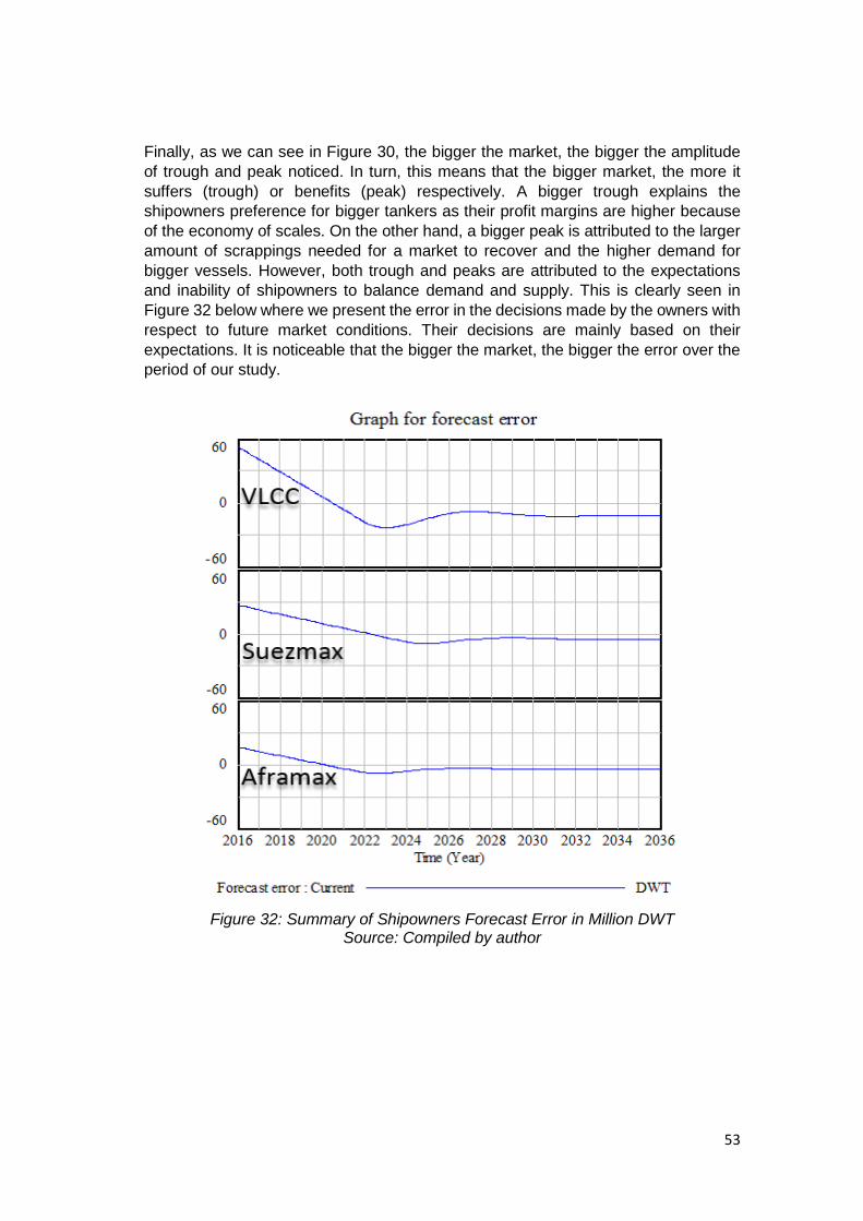
53

Finally, as we can see in Figure 30, the bigger the market, the bigger the amplitude

of trough and peak noticed. In turn, this means that the bigger market, the more it

suffers (trough) or benefits (peak) respectively. A bigger trough explains the

shipowners preference for bigger tankers as their profit margins are higher because

of the economy of scales. On the other hand, a bigger peak is attributed to the larger

amount of scrappings needed for a market to recover and the higher demand for

bigger vessels. However, both trough and peaks are attributed to the expectations

and inability of shipowners to balance demand and supply. This is clearly seen in

Figure 32 below where we present the error in the decisions made by the owners with

respect to future market conditions. Their decisions are mainly based on their

expectations. It is noticeable that the bigger the market, the bigger the error over the

period of our study.

Figure 32: Summary of Shipowners Forecast Error in Million DWT Source: Compiled by author

54

Chapter 8 Conclusions and Recommendations

8.1. Conclusions

This thesis deals with the dynamic interrelationships among the variables affecting

the performance of the crude tanker industry. After building a system dynamics

capacity model for the crude tanker industry, the performance of three different crude

tanker sectors is studied in order to draw conclusions about the performance and

eventual turning points of the overall crude tanker industry over the next 10 years.

More specifically, the crude tanker sectors under consideration are the VLCC,

Suezmax and Aframax sectors.

The cyclicality and uncertainty that governs the shipping industry has drawn the

attention of both academics and shipping professionals. Over the years, various

works have attempted to modelling and analyze the performance of the shipping

industry and the behaviour of its determinants. Our main research question of ‘’How

can we quantitatively assess the medium to long-term future of the crude oil tanker

market’’ motivated us to conduct the research herein.

To fully cover any aspect of our main research question, we had to answer four sub-

research questions. The purpose of the first sub-research question was to identify the

structure of the crude tanker market both in terms of its characteristics and the

different shipping markets with which is dealing. According to our research, there are

five different categories of crude tankers based on their size, which is commonly

measured in DWT. Starting with the largest one, the crude tankers are categorized

into ULCC, VLCC, Suezmax, Aframax and Panamax tankers. Each of these types of

tankers serves different routes because of its capacity and physical limitations of its

design. Therefore, it is apparent that different categories serve different demand, but

not always. The second part of the sub-question identifies four different shipping

markets with which the tanker industry is dealing. The shipping markets are

categorized into the Freight, Newbuilding, S&P and Demolition market. These

markets interact with each other affecting the performance of each shipping sector.

The purpose of the two next sub-questions is to identify the factors influencing the

supply of and demand for sea transport and the characteristics of shipping cycles.

Our research shows that the main factors affecting demand are the world economy,

the volume of seaborne trade, the average haul (distance of a trip) and random shocks

such as wars. On the other hand, supply is affected by the active world fleet, the

productivity of the vessels, which affects the supply in the short-term, and the

newbuilding and scrapping activity. With respect to the shipping cycles, they are

divided into the long, short and seasonal cycles. The shipping cycles have four distinct

stages, namely the trough, recovery, plateau/peak and collapse. Shipping cycles are

caused by imbalances in demand and supply. The imbalances can be attributed to

changes in world economy and various geopolitical events as well as to the irrational

behavior of shipowners in response to price signals and the time delay between

ordering and delivery of new ships. According to Stopford (2002), endogenous factors

trigger the shipping cycles, while the exogenous ones generate the cyclical pattern.

The shipping industry long-cycles usually last 20 years as the new vessels entering

the market are not destined to be scrapped before they reach their average lifetime,

55

which is twenty to twenty-five years. On the other hand, the short cycles can range

from 3 to 12 years depends on owners’ decisions such as the increase in vessels

speed which in turn increase the supply in the short-term. Lastly, the seasonal cycles

are caused by variations in demand of a specific commodity because of different

seasons.

Our analysis, made in chapter 5, shows that systems dynamics modelling is

appropriate for the purpose of our study because it considers delays in the balance

between supply and demand, changes in exogenous variables as well as the

continuous cause and causality relations that shape the tanker market over time. Our

last sub-research question has to do with the development of an appropriate system

dynamics model for assessing the future of the market. We constructed a system

dynamics capacity model for the crude tanker market in order to predict market turning

points in the next 10 years, studying the balance between supply and demand in terms

of DWT. Value added to the existing literature arises from this thesis by employing a

variable called forecast error which identifies the false expectations and as a result,

the false decisions made by shipowners. In essence, the forecast error shows the

inability of the shipowners to balance demand supply for seaborne transport over time.

In line with our main question, we run our model for a 20-year period in order to assess

the tanker market in the next ten years. Our findings show that Aframax and VLCC

bottom first in the second half of and late 2016 respectively, followed by Suezmax at

the end of 2016. Although all the different sectors seem to enter the trough stage

during 2016, the VLCC and Aframax sectors show recovery signs from the first half

of 2017, while Suezmax after the first half of 2018. Over the next years, Aframax

peaks first between the second half of 2023 and late 2024, followed by VLCC and

Suezmax in the whole 2024 and 2026 respectively. A striking feature arising from our

results is that all the different tanker markets follow the same pattern, although there

are differences in the time each sector bottoms and peaks, in the amplitude as well

as the in time horizon of peaking or bottoming.

From our findings, it arises that the main determinant of the peaks and bottoms

(troughs) is the level of the active fleet. Moreover, the bigger the market, the more it

benefits or suffers compared to the other tanker markets. Furthermore, since the

demand is projected to increase over the period we run the model, the forecast error

shows that the shipowners inability to balance demand and supply is responsible for

the future performance of each sub-market. Finally, the forecast error variable also

shows that the larger the market, the bigger the decision errors made by the owners

and thus, their inability to balance demand and supply.

56

8.2. Limitations

Having two months to complete our research, this thesis is subject to a number of

limitations. First of all, in our model we consider tankers in lay-up and tankers for

storage as part of the active fleet as it is difficult to quantify them. Moreover, we

employ a constant annual scrapping rate instead of calculating the scrapping activity

based on the year each vessel has to be scrapped. Another limitation of our model is

the rate of overordering we used. As we did not find available data about overordering

we used random numbers.

Our model is applied in times where there is no much noise in the market. We built

the model under the assumption that no geopolitical events, which can distort the

market, will occur over the time horizon of our study. This limitation is mainly attributed

to the software Vensim PLE which has no option for sensitivity analysis.

8.3. Recommendations for Further Research

An interesting recommendation for further research could be the application of our

model in the dry bulk market as well. As both dry bulks and tankers are part of the

bulk shipping, it would be interesting to compare the results and examine similarities

and differences observed in the behaviour of the tanker and dry bulk market as well

as in the shipowners forecast error.

Another interesting recommendation could be to quantify overordering in order for our

model to provide more accurate results. In addition, another development of our

model could be to build the model in that way that could calculate the scrapping

according to the time each ship should be scrapped at any time and not take a

constant scrapping rate.

We believe that there is much room for further research and development of our

model. We hope that further developments of our model could help not only academic

research but also shipping practitioners decision-making process.

57

Bibliography

Abouarghoub, W., Mariscal, I. B.-F. & Howells, P., (2012). 'Dynamic Earnings within

Tanker Markets: An Investigation of Exogenous and Endogenous Structure Breaks'.

American International Journal of Contemporary Research, 2(1), pp. 132-147.

Adland, R., Cariou, P. & Wolff, F.-C., (2016). 'The influence of charterers and

owners on bulk shipping freight'. Transportation Research Part E: Logistics and

Transportation Review, Volume 86, pp. 69-82.

Adland, R. & Cullinane, K., (2006). 'The non-linear dynamics of spot freight rates in

tanker markets'. Transportation Research Part E, 42(3), pp. 211-224.

Adland, R., Jia, H. & Koekebakker, S., (2004b). 'The Pricing of Forward Ship Value

Agreements and the Unbiasedness of Implied Forward Prices in the Second-Hand

Market for Ships'. Maritime Economics & Logistics, Volume 6, pp. 109-121.

Adland, R. & Siri P. Strandenes, (2004a). A Discrete-Time Stochastic Partial

Equilibrium Model of the Spot Freight Market (SNF Report No. 04/04), Bergen:

Centre for International Economics and Shipping, Institute for Research in

Economics and Business Administration.

Alizadeh, A. H. & Nomikos, N. K., (2009). Shipping Derivatives and Risk

Management. 1st ed. London: PALGRAVE MACMILLAN.

Beenstock, M. & Vergottis, A., (1989). 'An Econometric Model of the World Tanker

Market'. Journal of Transport Economics and Policy, 23(3), pp. 263-280.

Beenstock, M. & Vergottis, A., (1993). Econometric Modelling of World Shipping.

London: Chapman & Hall.

Berg-Andereassen, J. A., (1996). 'Some properties of international maritime

statistics'. Maritime Policy & Management, 23(4), pp. 381-395.

Berg-Andreassen, J. A., (1997). 'The relationship between period and spot rates in

international maritime markets'. Maritime Policy & Management, 24(4), pp. 335-350.

BIMCO, (2016). BIMCO. [Online]

Available at:

https://www.bimco.org/Reports/Market_Analysis/2016/0104_Reflections2016.aspx

Bloomberg News, (2016). Bloomberg. [Online]

Available at: http://www.bloomberg.com/news/articles/2016-07-15/china-s-oil-coal-

output-slides-in-sign-of-more-imports-to-come

BRS, (2016). 2016 Annual Review, Neuilly-sur-Seine: BRS Group.

Clarkson Research Services Limited, (2016). 'Oil & Tanker Trades Outlook, June

2016'. Clarksons Research, 21(6), pp. 1-28.

Clarkson Research Services Limited, (2016). 'Seaborne Trade Monitor, May 2016'.

Clarksons Research, 3(5), pp. 1-11.

Clarksons Shipping Intelligence Network, (2016). Fleet, London: Clarksons.

58

Clarksons Shipping Intelligence Network, (2016). Orderbook, London: Clarksons.

Dikos, G., Marcus, H. S., Papadatos, M. P. & Papakonstantinou, V., (2006). 'Niver

Lines: A System-Dynamics Approach to Tanker Freight Modeling'. Interfaces, 36(4),

pp. 326-341.

EIA BETA, (2016). EIA. [Online]

Available at:

http://www.eia.gov/beta/MER/index.cfm?tbl=T11.01B#/?f=A&start=2000&end=2015

&charted=0-11-12

EIA, (2016). Independent Statistics & Analysis U.S. Information Administration.

[Online]

Available at: http://www.eia.gov/todayinenergy/detail.cfm?id=24532

Engelen, S., Meersman, H. & Voorde, E. V. D., (2006). 'Using system dynamics in

maritime economics: an endogenous decision model for shipowners in the dry bulk

sector'. Maritime Policy & Management, 33(2), pp. 141-158.

George Dikos, H. S. M. a. M. P. P., (2007). 'Old Ideas May Still be New: A System

Identification Approach to Tanker Freight Modelling'. Wiley InterScience, Issue 24,

pp. 627-644.

Glen, D. R., (2006). 'The modelling of dry bulk and tanker markets: a survey'.

Maritime Policy & Management, 33(5), pp. 431-445.

Glen, D. & Rogers, P., (1997). 'Does Weight matter? A Statistical analysis of the

SSY Capesize index'. Maritime Policy & Management, 24(4), pp. 351-364.

Goulielmos, A., (2009). 'Risk analysis of the Aframax freight market and of its new

building and second hand prices, 1976-2008 and 1984-2008'. International Journal

of Shipping and Transport Logistics, 1(1), pp. 74-79.

Hamilton, J. D., (2008). 'Understanding Crude Oil Prices'. Energy Policy and

Economics, 30(2), pp. 179-206.

Hawdon, D., (1978). 'Tanker freight rates in the short and long run'. Applied

Economics, 10(3), pp. 203-17.

IHS, (2014). US Crude Oil Export Decision Assessing the impact of the export ban

and free trade on the US economy, Houston, Texas: IHS.

IMO, n.d. About IMO. [Online]

Available at: http://www.imo.org/en/About/Pages/Default.aspx

International Maritime Organization IMO, (2016). IMO International Maritime

Organization. [Online]

Available at:

http://www.imo.org/en/OurWork/Environment/PollutionPrevention/OilPollution/Pages

/constructionrequirements.aspx

Jugović, A., Komadina, N. & Hadžić, A. P., (2015). 'Factors influencing the formation

of freight rates on maritime'. Scientific Journal of Maritime Research, Issue 29, pp.

23-29.

59

Kavussanos, M. G., (1997). 'The dynamics of time-varying volatilities in different size

second-hand ship prices of the dry-cargo secto'r. Applied Economics, 29(4), pp.

433-443.

Kavussanos, M. G. & Alizadeh, A. H., (2002). 'Efficient pricing of ships in the dry

bulk sector of the shipping industry'. Maritime Policy & Management, 29(3), pp. 303-

330.

Knapp, S., Kumarb, S. N. & Remijn, A. B., (2008). 'Econometric analysis of the ship

demolition market'. Marine Policy, 32(6), p. 1023–1036.

Koekebakker, S. & Adland, R., (2004). 'Modelling forward freight rate dynamics—

empirical evidence from time charter rates'. Maritime Policy & Management, 31(4),

pp. 319-335.

Koekebakker, S., Adland, R. & Sødal, S., (2006). 'Are Spot Freight Rates

Stationary?'. Journal of Transport Economics & Policy, 40(3), pp. 449-472.

Koopmans, T., (1939). Tanker Freight Rates and Tankship Building, An Analysis of

cyclical fluctuations report No. 27, Haarlem, De erven F. Bohn NV: Netherlands

Economic Institute.

Niko Wijnolst, F. W., (1999). 'Shipping Industry Structure'. Delft: Delft University

Press.

Norman, V., (1979). Economics of bulk shipping, Bergen, Norway: Institute for

Shipping Research.

Norman, V. & Wergeland, T., (1981). Nortank - A Simulation Model of the Freight

Market for Large Tanker (Report 4/81), Bergen: Centre for Applied Research,

Norwegian School of Economics and Business Administration.

Randers, J. & Göluke, U., (2007). 'Forecasting turning points in shipping freight

rates: lessons from 30 years of practical effort'. Systems Dynamics Review, 23(2-3),

pp. 253-284.

Roar Adland, K. C., (2006). 'The non-linear dynamics of spot freight rates in tanker

markets'. Transportation Research Part E, Issue 42, pp. 211-224.

Schuit, K., (2004). CYCLICALITY IN THE TANKER INDUSTRY. Dr. Thesis,

Rotterdam, The Netherlands: Erasmus University Rotterdam.

Sen, A. & Sen, A., (2016). India’s Oil Demand:On the Verge of ‘Take-Off’?-OIES

PAPER: WPM 65, Oxford: Oxford Institute for Energy Studies.

Sterman, J. D., (2000). BUSINESS DYNAMICS:Systems Thinking and Modeling for

a Complex World. New York: McGraw-Hill.

Stopford, M., (2002). Shipping Market Cycles. In: C. T. Grammenos, ed. The

Handbook of Maritime Economics and Business. London: LLP, pp. 203-224.

Stopford, M., (2009). Maritime Economis. 3rd ed. New York: Routledge Taylor &

Francis Group.

60

Strandenes, R. A. a. S. P., (2004). A discrete-time stohastic partial equilibrium

model of the spot freight market, Bergen: SIOS-Centre for International Economics

and Shipping.

Strandenes, S., (1986). NORSHIP - A Simulation Model for Bulk Shipping Markets,

Bergen: Centre for Applied Research, Norwegian School of Economics and

Business Administration.

Strandenes, S., (2002). Economics of the markets for ships. In: C. T. Grammenos,

ed. The handbook of maritime economics. London: LLP.

Taylor, A. J., (1976). 'System Dynamics in Shipping'. Operational Research

Quarterly (1970-1977), 27(1), pp. 41-56.

The guardian, (2016). theguardian. [Online]

Available at: https://www.theguardian.com/business/2016/feb/07/north-sea-oil-rigs-

could-be-scrapped-in-10-years

The World Bank, (2016). THE WORLD BANK IBRD-IDA. [Online]

Available at: http://data.worldbank.org/topic/economy-and-growth

Tsolakis, S., (2005). Econometric Analysis of Bulk Shipping Markets Implications for

Investment Strategies and Financial Decision-Making. Dr. Thesis, Rotterdam, The

Netherlands: Erasmus University Rotterdam.

Tvedt, J., (1997). 'Valuation of VLCCs under income uncertainty'. Maritime Policy &

Management, 24(2), pp. 159-174.

U.S. Energy Information Administration, (2016). Independent Statistcs & Analysis

U.S. Energy Information Administration. [Online]

Available at: https://www.eia.gov/finance/markets/supply-opec.cfm

UNCTAD, (2015). REVIEW OF MARITIME TRANSPORT 2015, New York and

Geneva: UNITED NATIONS.

Veenstra, A. & Ludema, M., (2003). Cyclicality in Ocean Tanker Shipping. s.l., The

International Workshop on Harbour, Maritime & Multimodal Logistics Modelling and

Simulation.

Veenstra, A. W., (1999a). Quantitative analysis of shipping markets, Delft: Delft

University Press.

Veenstra, A. W., (1999b). 'The term structure of ocean freight rates'. Maritime Policy

& Management, 26(3), pp. 279-293.

Veenstra, A. W. & Fosse, S. D. L., (2006). 'Contributions to maritime economics—

Zenon S.'. Maritime Policy & Management, 33(1), pp. 61-73.

Wijnolst, N. & Wergeland, T., (1996). Shipping. Delft: Delft University Press.

Worldscale Association, (2016). Worldscale. [Online]

Available at: https://www.worldscale.co.uk/contentmanagement/viewassinglepage

Zannetos, Z. S., (1966). The Theory of Oil Tankship Rates. Cambridge: MIT Press.

61

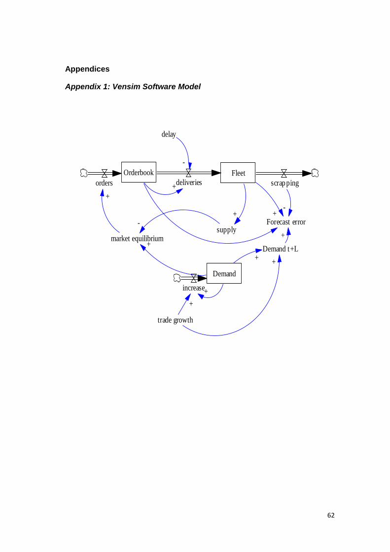
62

Appendices

Appendix 1: Vensim Software Model

Orderbook Fleet

orders deliveries scrapping

supply

+

market equilibrium

-

+

Demand

increase

trade growth

+

+

+

delay

-

+

Demand t+L+

Forecast error

+

+

+

-

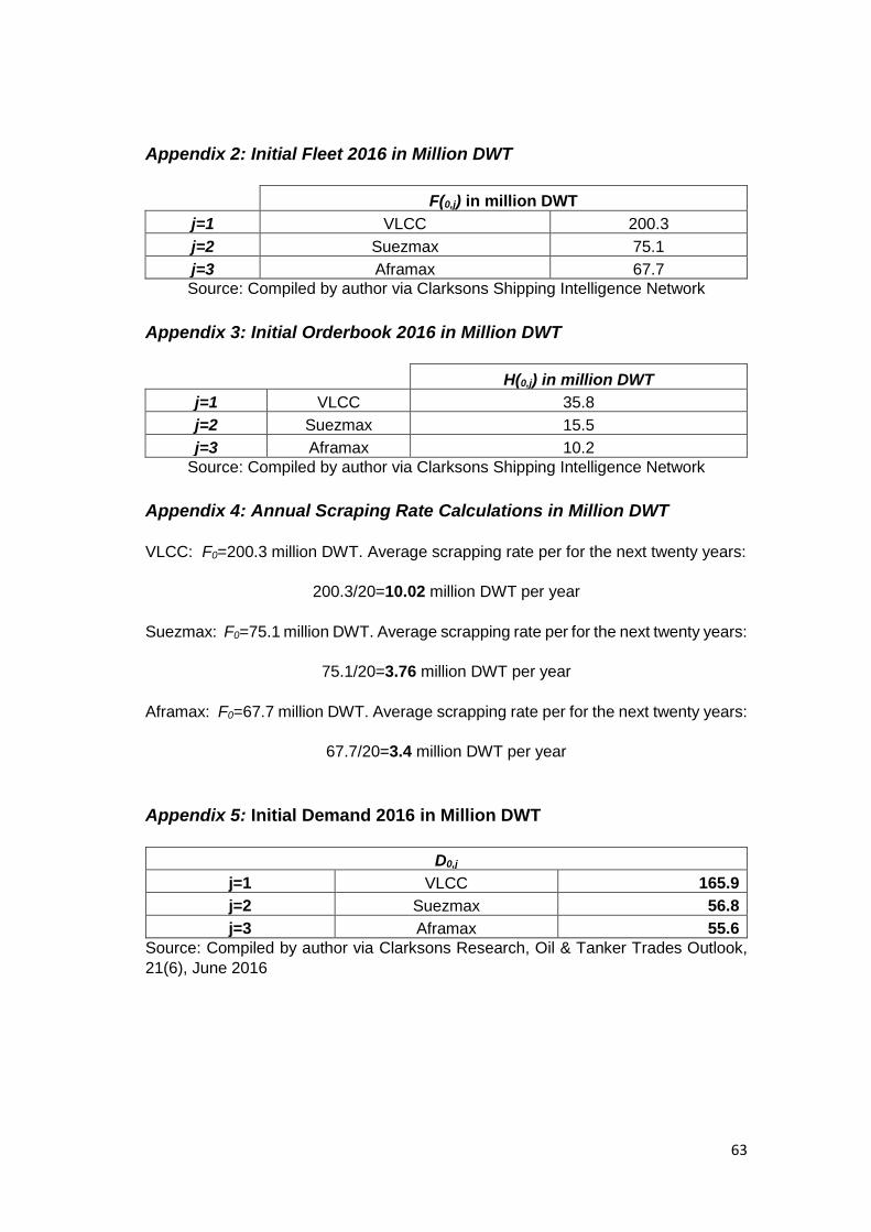
63

Appendix 2: Initial Fleet 2016 in Million DWT

F(0,j) in million DWT

j=1 VLCC 200.3

j=2 Suezmax 75.1

j=3 Aframax 67.7

Source: Compiled by author via Clarksons Shipping Intelligence Network

Appendix 3: Initial Orderbook 2016 in Million DWT

H(0,j) in million DWT

j=1 VLCC 35.8

j=2 Suezmax 15.5

j=3 Aframax 10.2

Source: Compiled by author via Clarksons Shipping Intelligence Network

Appendix 4: Annual Scraping Rate Calculations in Million DWT

VLCC: F0=200.3 million DWT. Average scrapping rate per for the next twenty years:

200.3/20=10.02 million DWT per year

Suezmax: F0=75.1 million DWT. Average scrapping rate per for the next twenty years:

75.1/20=3.76 million DWT per year

Aframax: F0=67.7 million DWT. Average scrapping rate per for the next twenty years:

67.7/20=3.4 million DWT per year

Appendix 5: Initial Demand 2016 in Million DWT

D0,j

j=1 VLCC 165.9

j=2 Suezmax 56.8

j=3 Aframax 55.6

Source: Compiled by author via Clarksons Research, Oil & Tanker Trades Outlook,

21(6), June 2016

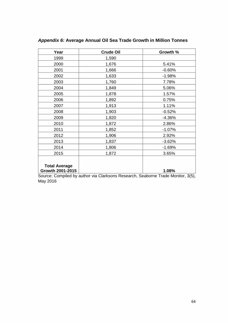
64

Appendix 6: Average Annual Oil Sea Trade Growth in Million Tonnes

Year Crude Oil Growth %

1999 1,590

2000 1,676 5.41%

2001 1,666 -0.60%

2002 1,633 -1.98%

2003 1,760 7.78%

2004 1,849 5.06%

2005 1,878 1.57%

2006 1,892 0.75%

2007 1,913 1.11%

2008 1,903 -0.52%

2009 1,820 -4.36%

2010 1,872 2.86%

2011 1,852 -1.07%

2012 1,906 2.92%

2013 1,837 -3.62%

2014 1,806 -1.69%

2015 1,872 3.65%

Total Average Growth 2001-2015 1.08%

Source: Compiled by author via Clarksons Research, Seaborne Trade Monitor, 3(5),

May 2016