DBJ Discussion Paper Series, No.1210

What Determines CDS Prices?

Evidence from the Estimation of Protection Demand and Supply

Daisuke Miyakawa (Development Bank of Japan)

And

Shuji Watanabe (Nihon University)

December 2012

Discussion Papers are a series of preliminary materials in their draft form. No quotations,

reproductions or circulations should be made without the written consent of the authors in

order to protect the tentative characters of these papers. Any opinions, findings,

conclusions or recommendations expressed in these papers are those of the authors and do

not reflect the views of the Institute.

白紙

- 1 -

What Determines CDS Prices?

Evidence from the Estimation of Protection Demand and Supply

December 2012

Daisuke Miyakawa† and Shuji Watanabe‡

Development Bank of Japan and Nihon University

Abstract

This paper examines the determinants of Credit Default Swap (CDS) premiums by applying a

limited dependent variable simultaneous equation system to a unique set of time-series data for the

Japanese credit market. The estimation results indicate that CDS premiums decrease as a result of an

increase in the supply of protection due, for example, to fewer opportunities for investment in other

assets (e.g., loans). We also find that premiums increase when the demand for protection increases

due, for example, to larger short cover needs. Further, the quantitative impact of factors accounting

for the supply and demand of protection is likely to be misestimated unless the simultaneous

determination of supply and demand is taken into account. This indicates that it is necessary to

include demand and supply factors to understand fluctuations in CDS premiums.

Key words: Credit Default Swap; Demand and Supply; Simultaneous Equation; Credit Link Note

JEL Classification: G12, C34, C36,

We thank would like to thank Tatsuyoshi Okimoto (Hitotsubashi University), Takayoshi Kitaoka (Meiji University), Kentaro Akashi (Gakushuin University), Hiroaki Yamauchi (MTEC), Masazumi Hattori (Bank of Japan), Toyoichiro Shirota (Bank of Japan), Robert Dekle (University of Southern California), and seminar participants at the Research Institute of Capital Formation, the Development Bank of Japan (RICF-DBJ), the Japan Society of Monetary Economics 2012 spring meeting, the Nippon Finance Association 2012 annual meeting, and the Bank of Japan Institute of Monetary and Economic Studies Seminar for helpful suggestion. We are also grateful to Takeshi Moriya for excellent research assistance. † Corresponding Author, Associate Senior Economist, Research Institute of Capital Formation, Development Bank of Japan, 1-9-3 Otemachi Chiyoda-ku, Tokyo, 100-0004 Japan. Phone: +81-3-3244-1917. E-mail: damiyak@dbj.jp. ‡ Professor, College of Economics, Nihon University, 1-3-2 Misaki-cho, Chiyoda-ku, Tokyo 102-8360 Japan. E-mail: watanabe.shuji@nihon-u.ac.jp.

- 2 -

1. Introduction

Credit default swaps (CDS) are a type of credit derivatives written against the default of a

specific firm, security, country, or a basket of these. They function as an insurance against default

events and have been widely used as a hedging tool as well as a speculation tool in recent years.

However, during the recent financial crisis, substantial turmoil in CDS markets could be observed.

Indexes of CDS spreads (i.e., the premium paid for protection) in the United States, Europe, and

Japan show large jumps from early 2008 onward in response to the financial crisis triggered by the

malfunctioning of U.S. credit markets, which was accompanied by a sharp decline in the prices of

securitized products based on various underlying assets.

Given the growing presence of CDSs in financial markets and such large fluctuations in

CDS premiums, many academic researchers and practitioners have been trying to establish the

determinants of such premiums. The list of candidates includes macro and micro credit factors (e.g.,

stock prices and bond prices) directly affecting the default probability of the entities referenced by

CDSs as well as factors relatively specific to credit markets (e.g., counter-party risk, market

segmentation, illiquidity). Thanks to the research effort into the mechanisms governing CDS markets,

the role of the various determinants is now largely understood. However, an issue that has received

surprisingly little attention in this context so far is the role played by the demand for and supply of

protection through CDSs. Against this background, the aim of the present paper is to examine the

determinants of CDS premiums explicitly taking such demand and supply into account.

The empirical strategy employed in the large majority of extant studies has been to regress

the CDS premium on various covariates representing factors accounting for credit and liquidity in a

single equation (e.g., Huang et al. 2003; Blanco et al. 2005; Scheicher 2008; Ericsson et al. 2009). In

other words, CDS premiums have been considered as a measure of the default risk and assumed not

be affected by the demand for and supply of CDSs. In contrast, the present study explicitly

introduces the notion of demand and supply, which has been widely considered as a key determinant

of prices in other financial markets such as stock, government and corporate bond, and foreign

exchange markets. Specifically, we examine how the interaction of the demand for and supply of

protection affects an index of CDS premiums in the Japanese credit market.

While it is relatively easy to measure the price of protection using indexes of premiums in

CDS markets (e.g., the various indexes provided by Markit Group Ltd. such as the iTraxx Japan for

the Japanese credit market), the quantity of CDS transactions is more difficult to observe. It is

particularly difficult to obtain information on the volume of each transaction, mainly due to the lack

of a central clearing system. This is the biggest reason making it difficult to study the demand for

and supply of protection. We should note, however, that most of the transactions among market

makers, which account for the majority of transactions, are offset in a relatively short period by

transactions in the opposite direction. This reflects the intention of market makers to “square” their

- 3 -

positions as soon as possible.1 Our empirical strategy in this paper is to take advantage of this

feature and exclusively focus on the flow in trades for “outright” protection, which account for

positions held for a long period. We use the issuance volume of credit linked notes (CLNs), which

are securitized products written against CDSs, as a proxy for the trade flow in outright protection.

Due to the lack of a secondary market and high transaction costs, the standard investment strategy

for CLNs is “buy-and-hold,” which assures that the trade for protection associated with the CLN

investments tends to be held for a long period, mostly until their maturity.

An additional technical problem originating from the use of CLN data is that we observe

a large number of zero amounts of CLN issuance. This is partly because most of the CLNs are

tailor-made and incur time and costs to deliver. Moreover, investors in CLN are relatively limited. To

deal with such truncated data, we employ a simultaneous equation Tobit model of the type first

proposed by Nelson and Olson (1978) and refined by Amemiya (1979).

Our estimation shows that not considering the simultaneous equation system likely results

in substantial misestimation of the impact of changes in the exogenous shift variables for the

protection supply and demand curves. This could be interpreted as a sign of simultaneity bias in the

reduced form regression. Our estimation also shows that the impact of some factors on CDS

premiums could not be identified when we do not properly take the truncated sample into account.

These results imply that, to examine the determinants of CDS spreads, it is necessary to explicitly

consider demand and supply as well as the potential bias originating from the limited dependent

variable (i.e., the truncated data on transaction volumes).

The remainder of the paper is organized as follows. The next section provides an overview

of the basic structure of CDSs and the related securitized products markets. Section 3 briefly surveys

the literature on the determinants of CDS premiums. Section 4 then describes the data and the

empirical framework used for our analysis, while Section 5 discusses the results. Section 6 concludes

and highlights remaining issues.

2. Basics of Credit Default Swap Markets and Credit Linked Notes

Figure 1 provides a conceptual depiction of the CDS market. Transactions in CDSs, that

is, the selling and buying of protection, can take place between (i) outright protection sellers and

market makers, (ii) outright protection buyers and market makers, and (iii) among market makers

themselves. Almost all the transactions are executed as over-the-counter (OTC) transactions and

1 That transactions are typically largely offset within brief periods is illustrated by the following quotes from a recent Bloomberg article: “JPMorgan purchased single-name contracts protecting $147.3 billion of debt and sold $142.4 billion related to the so-called GIIPS nations of Greece, Ireland, Italy, Portugal and Spain.” Moreover: “JPMorgan said ‘master netting agreements’ reduced the notional amount of protection purchased to $18.5 billion and the amount sold to $13.7 billion.” (Source: Bloomberg.com, February 29, 2012, “Goldman Mirrors JPMorgan Mirrors Goldman on Swap Exposure to European Debt,” sic).

- 4 -

cannot be easily tracked.2 Since most of the transactions among market makers are squared in short

periods, however, the transaction volume in CDS markets which affects the CDS premium is likely

to be mainly affected by transactions in outright protection, which are proxied by the issuance

volume of CLNs.

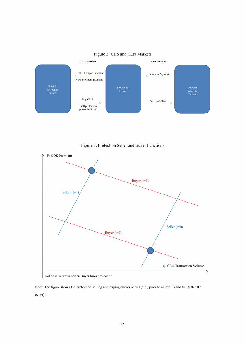
CLNs are securities that resemble bonds and provide fixed coupon payments to their

holders. 3 Figure 2 illustrates how CLNs and CDSs are linked. The right-hand side shows

transactions in CDSs, which take place between securities firms and outright protection buyers.

Securities firms play the role of sellers of protection against some default event and receive a

premium in return. Outright buyers buy the protection and use it, for example, to hedge the credit

risk in their portfolio or to buy protection with a speculative motive.4 Next, the left-hand side shows

transactions in CLNs, which are originated by the securities companies and sold to outright

protection sellers, who receive the coupon on the CLNs, which is based on the premium associated

with the CDSs and the return on the invested principal. In this sense, the demand for and supply of

CLNs are accompanied by protection selling and buying, respectively. The coupon payment may be

contingent on a default event relating to a specific company, or a range of companies. Moreover, the

contingency may be designed in a variety of ways.5,6 An important feature is that the CLN

investment positions are in general held for a long period due to the lack of a secondary market for

CLNs and high transaction costs. This is the reason why it is appropriate for our analysis to measure

outright transactions in CDSs based on CLN issuance data.

A graphic representation of what our empirical study seeks to examine is presented in

Figure 3. In the diagram, the volume of CDS transactions, proxied by the issuance of CLNs, is

plotted on the horizontal axis, while the price, proxied by the iTraxx Japan index for CDS premiums,

is plotted on the vertical axis. Suppose that protection sellers (i.e., CLN investors = outright

protection sellers) have a large capacity for investing in CLNs and outright protection buyers do not

show large demand for protection. Under such circumstances, the spread would be tight, since the

supply of protection is large, while the demand for protection is limited. However, if, for example,

the perceived risk of investing in CLNs increased, the protection seller curve would shift upward

(i.e., t=1), since the appetite for CLN investment becomes smaller. Similarly, the protection buyer

2 That being said, data on individual CDS transactions is increasingly being disclosed (e.g., by the Depository Trust & Clearing Corporation (DTCC)), but the amount of data accumulated on such transactions to date is insufficient for analytical purposes. For Japan, the BOJ has been releasing data on CDS transaction volumes aggregated for each six-month period. 3 Synthetic collateralized debt obligations (CDOs) are included in the CLNs considered in this paper. Note also that some CLNs have floating coupon payments, but the number of such cases is limited. 4 Investors may buy CDSs for speculative purposes rather than for protection. In this case, they aim to make a profit by buying CDSs when premiums are low and selling them when premiums are high. 5 Most CLNs are sold in units of 2 billion yen and are highly customized to suit each investor’s preferences. 6 As a typical example, the coupon payment to investors in CLNs categorized as first-to-default (FTD) is terminated and only part of the principal of the CLNs is paid back to investors when one of the firms referenced by the CLN contract defaults. The rise of CLNs in the Japanese credit market is largely driven by the issuance of such FTD-type CLNs.

- 5 -

curve would shift up when, for example, the demand for protection increases due to a larger need for

risk hedging (i.e., t=1).7 We conjecture that the sharp rise in CDS spreads during the recent financial

crisis actually emerged due to such shifts in both protection selling and buying.

There have been many investors in Japan who require products with higher risks and

higher returns than offered by traditional investment assets (e.g., Japanese government bond). Over

the last decade, securities firms have been providing various securitized products such as mortgage

backed securities (MBS) and CLNs to investors with a high risk-return appetite. This rising demand

for securitized products has led securities firms to sell protection in CDS markets to procure the

underlying assets for securitized products. One of our main conjectures is that such demand pressure

in the securitized products markets, which works as supply pressure in the CDS market, plays a

central role in the determination of premiums in the CDS market.

3. Related Literature

The pricing implications of imbalances in supply and demand have received considerable

attention in theoretical studies on CDS markets (e.g., Bollen and Whaley 2004; Brunnermeier and

Pedersen 2009; Garleanu et al. 2009). However, when it comes to empirical studies on CDS pricing,

despite their substantial number (e.g., Huang et al. 2003; Longstaff et al. 2005; Ericsson et al. 2009;

Scheicher 2008), there are hardly any that explicitly that take into account the notion of supply and

demand. A notable exception is the study by Tang and Yan (2011), which employs the difference

between the number of bids and offers as a proxy for imbalances in supply and demand. They show

that such imbalances have a statistically significant and sizable impact on CDS spreads. Similar to

the approach taken in this paper, they attempt to take into account the simultaneous determination of

CDS prices and transaction volumes by using two-stage least squares estimation. The present study

takes the analysis a step further and explicitly examines shifts in the protection seller and buyer

curve and the impact of such shifts on CDS spreads – something that is not discussed in Tang and

Yan’s (2011) study.

While the impact of supply and demand imbalances in CDS markets has remained largely

unexplored, this is not the case for other financial markets. Starting from the pioneering study by

Kraus and Stoll (1972), numerous studies, such as Chordia et al. (2002), Chordia and Subramanyam

(2004), Coval and Stafford (2007), Sarkar and Schwartz (2009), and Hendershott and Menkveld

(2012) have examined and confirmed the impact of supply and demand and on stock prices.

Similarly, Greenwood and Vayanos (2010) and Krishnamurthy and Vissing-Jorgenson (2012) have

examined the role of supply and demand in the determination of government bond prices, while Ellul

et al. (2011) did the same for corporate bond prices. Against this background, the role of supply and

7 We will provide more details on the mechanisms further below.

- 6 -

demand in the determination of CDS prices remains an important gap in the literature, which the

present study seeks to fill.

4. Data and Empirical Framework

4.1. Data and Hypotheses

This section provides a description of the data we use for our empirical analysis and sets

out our hypotheses. We begin by describing our data. As our variable representing CDS premiums,

we use the Markit iTraxx Japan (iTraxx_P) index. This is an index of the CDS premium in the

Japanese credit market and consists of a basket of five-year CDSs for 50 investment-grade Japanese

firms with the highest market liquidity.8 This index, which is updated daily, is computed from the

spreads reported by licensed market makers.

In contrast with the ready availability of such price data, data on the quantity of CDS

transactions is difficult to obtain due to the lack of a centralized clearing system. Therefore, we

instead use data on the issuance of CLNs (CLN_ISSUE_Q) from January 2002 to March 2011, which

we collected from information released by Rating and Investment Information Inc. (R&I).

Specifically, the data on CLN issuance that we use for our empirical analysis consist of roughly 400

issuances worth almost 1.1 trillion yen. We exclude two large issuances, that by Bank of Tokyo

Mitsubishi UFJ in 2006 and that by Mizuho Corporate Bank in 2009, as outliers.9 We construct

weekly frequency data and compute the moving average of CLN_ISSUE_Q, since the impact of

CLN issuance on the CDS market is presumably not limited to the exact date of issuance but also

extends to adjacent periods. This could be the case when, for example, the timing of the CDS

transactions associated with the origination of CLNs are spread around the date of CLN issuance.

Note that there are still a large number of zeros for CLN_ISSUE_Q in our dataset after taking the

moving average. For consistency with the quantity data, we therefore transform the daily iTraxx

Japan data into weekly data by taking the average for each week.

As detailed in the next subsection, we model price determination in the CDS market as an

equilibrium between protection selling and buying. Specifically, we consider traditional investors in

the Japanese credit market such as Japanese domestic banks and various institutional investors as

outright protection sellers. To measure their risk-taking capacity, we use the level of the Nikkei 225

Stock Index (NKY_AVG). In order to take the average investment return on alternatives to

investments in CLNs into account, we use the five-year yield on Japanese government bonds

(JGB_5Y). Another variable we include is the average change in credit ratings of existing CLNs. To

8 The reasons that we focus on the Markit iTraxx Japan index rather than the CDS premium for each of the 50 firms are twofold. First, it is difficult to map the information on CLN issuance for each CLN issue to the referenced individual firms. Second, the Markit iTraxx Japan index is traded in the market as an individual investment tool. 9 These two synthetic CDOs were issued for risk hedging against the banks’ loan portfolios.

- 7 -

precisely measure the impact of rating changes, we multiply the issuance amount of each CLN by

the concurrent change in the rating of the CLN, the latter of which takes one (minus one) when the

CLN is downgraded (upgraded) by one notch.10 We conjecture that a larger value of this variable

(RATING_CHANGE) is associated with a higher credit risk of the CLN portfolio, which leads

protection sellers to require a higher premium and to be more cautious about any additional

investment. Protection sellers’ investment attitude may also be related to the availability of loan

investments. Suppose banks face a very low level of loan demand and need to find alternative

investment opportunities. In this case, such investors may be willing to sell protection at a relatively

low premium. To take this conjecture into account, we use the aggregate-level loan-to-deposit ratio

of commercial banks (LOAN_DEPOSIT) reported by the Bank of Japan as another exogenous shifter

of the protection seller curve. The hypothesis we test for these variables is as follows:

Hypothesis 1: The upward-sloping protection seller curve shifts upward (i.e., protection sellers are

willing to sell less protection at the same premium as before) when NKY_AVR decreases (investors’

risk-taking capacity decreases), JGB_5Y increases (the returns on other investments increase),

RATING_CHANGE increases (the risk of holding CLNs increases), and/or LOAN_DEPOSIT

increases (business opportunities in commercial banks’ main business improve).

We assume that speculative investors such as hedge funds and investment banks are the

buyers of outright protection. As factors shifting the protection buyer curve, we use the difference

between three-month dollar Libor (London inter-bank offered rate) and the three-month yield of U.S.

treasury bills (LIBOR_TREASUR3M), which we regard as a measure of the marginal funding cost of

financial institutions and which can be seen as a measure of risk in financial markets. We conjecture

that higher risk in the future as measured by a higher LIBOR_TREASUR3M leads speculative

investors to buy protection, which results in an upward shift of the protection buyer curve.

We also measure the change in the potential losses or gains from CLN purchased at time s

as of the current period t (MARK_TO_MKT). For simplicity, we assume that the maturity of all

CLNs is 5 years, which means that all of the existing CLNs have been issued during the five years

preceding t.11 Since a CLN issued at time s matures five years after s, semi-annual coupon

payments are made at time s k/2 k 1,2,⋯ ,10 . We denote the number of coupon payments

on a CLN issued at time s during the period t to s 5 by X s, t . Thus, MARK_TO_MKT is

expressed as the product of (i) the principal of the CLN issued at s (A ), (ii) the price change

between the issuance date s and t P P , and (iii) X s, t .12 Since the existing CLNs at time

10 An upgrade by one notch means, for example, a change from A to A+. 11 We focus on the potential losses and gains on CLNs with a maturity of 5 years, since these are the most actively traded CLNs in the CDS market. 12 For simplicity, we further assume that 1year consists of 52 weeks.

- 8 -

were issued during the period from 5 to , we aggregate this measure over these periods to

construct MARK_TO_MKT.13

As MARK_TO_MKT becomes negative, the potential losses for CLN holders become

larger (i.e., if the CLNs issued at time have a very low coupon rate, investors incur large losses at

time ). We conjecture that the protection buyer curve shifts up as this value falls. This would be the

case when securities firms, which are assumed to square their positions, buy more protection because

their sell-position against outright protection buyers is incurring losses. Such losses require securities

firms to provide additional collateral to the outright protection buyers in order to fulfill the CDS

contract (i.e., the counter-party risk increases for the original outright buyer). However, the securities

firms are not allowed to use the principal of the CLNs they received when the CLNs were issued.

Rather, the securities firms are required to hold the principal as collateral in case an actual credit

event occurs and the firm referenced by the CLNs defaults. In order to obtain funds they can use as

additional collateral, securities firms can buy protection (i.e., short cover) and obtain the collateral

from the new protection seller in the transaction. In addition, the securities firms may want to

procure the protection in advance to prepare for the selling request from original outright protection

buyers. In any case, the existence of such “new” protection buyers generates an upward shift of the

protection buyer curve. The hypothesis relating to the protection buyer curve can thus be stated as

follows:

Hypothesis 2: The downward-sloping protection buyer curve shifts upward (i.e., protection buyers

are willing to buy more protection for the same protection fee) when LIBOR_TREASUR3M

increases (protection buyers have a stronger speculative motive for buying protection) and/or

MARK_TO_MKT decreases (protection buyers have a stronger short-cover motive).

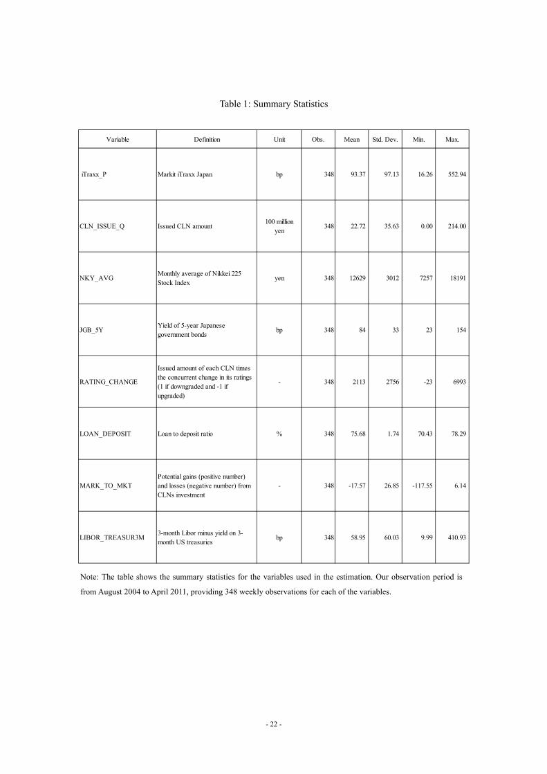
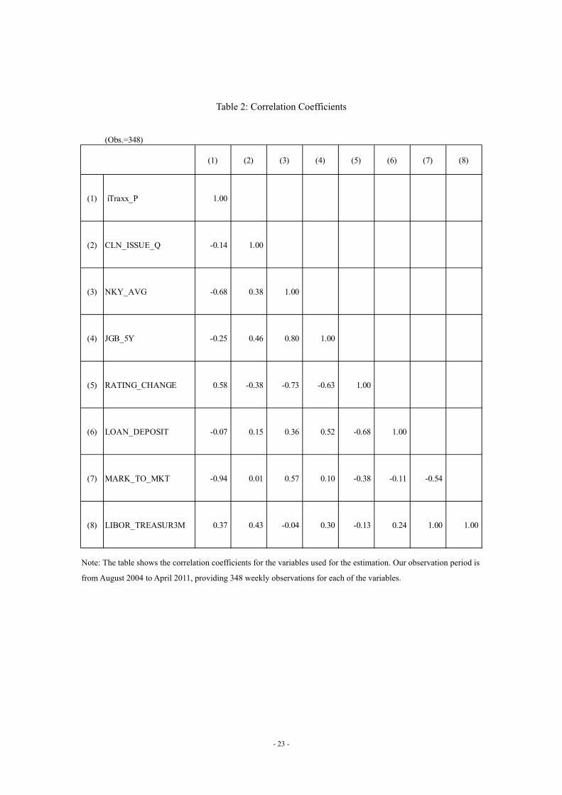
A full list of the variables we use in our estimation, their definitions, and summary

statistics is provided in Table 1. Further, Table 2 presents the correlation coefficients between the

various variables. Our observations cover the period from August 2004 to April 2011, spanning a

total of 348 weeks.

4.2. Empirical Framework

Our goal in this paper is to estimate the supply and demand functions of protection with

non-truncated price data (P: iTraxx_P) and truncated quantity data (Q∗: CLN_ISSUE_Q). For this

purpose, we consider a two-equations model consisting of equations 1 1 and 1 2 , where

the first equation represents the seller function and the second represents the buyer function. As we

13 Given the large variation of P P , we apply a monotonic transformation to P P by using the product of (i) the sign of P P and (ii) the square root of the absolute value of P P , instead of simply using P P .

- 9 -

detailed above, Q∗ is truncated at zero. Q∗ takes a positive value when CLNs are issued in the

week, and zero otherwise. Specifically, the model looks as follows:

P γ Q∗ X β u 1 1

Q∗ γ P X β u 1 2

ifQ Q∗ 0, Q∗ 0

Here, X represents the exogenous shift variables for the protection seller curve (i.e.,

NKY_AVR, JGB_5Y, RATING_CHANGE, and LOAN_DEPOSIT), while X represents the

exogenous shifters for the protection buyer curve (i.e., LIBOR_TREASUR3M and MARK_TO_MKT).

This system is identical to the model proposed by Nelson and Olson (1978) and refined by Amemiya

(1979). Note that if we did not need to take into account the limited dependent variable Q∗, we

could simply run the usual two-stage least squares estimation for the simultaneous equation system.

However, in order to deal with the fact that CLN issuance often takes a zero value, we need to use

the model above.

As explained in detail by Nelson and Olson (1978) and Amemiya (1979), the predicted

values of the endogenous variables are estimated using OLS or MLE in the first-stage regression.

The parameters Π ,Π in the reduced-form equations 2 1 and 2 2 , which represent the

coefficients associated with all the exogenous variables X, are estimated from this first-stage

regression as follows:14

P XΠ v 2 1

Q∗ XΠ v 2 2

ifQ Q∗ 0, Q∗ 0

where

Variance Covariancematrixof v , v

As in Amemiya (1979), the results of the first-stage regression Π ,Π , where Π and

Π are respectively the OLS and Tobit MLE estimates, are used to estimate the structural

parameters γ , γ , β , β . Note that u v γ v and u v γ v need to be satisfied so

that 1 1 and 1 2 are identified from 2 1 and 2 2 . Substituting the results from

2 2 into 1 1 yields the following expression, which provides us with α through standard

OLS estimation:

14 A similar issue is discussed in the paper by Keshk (2003), which explains the Stata command for simultaneous equation probit models.

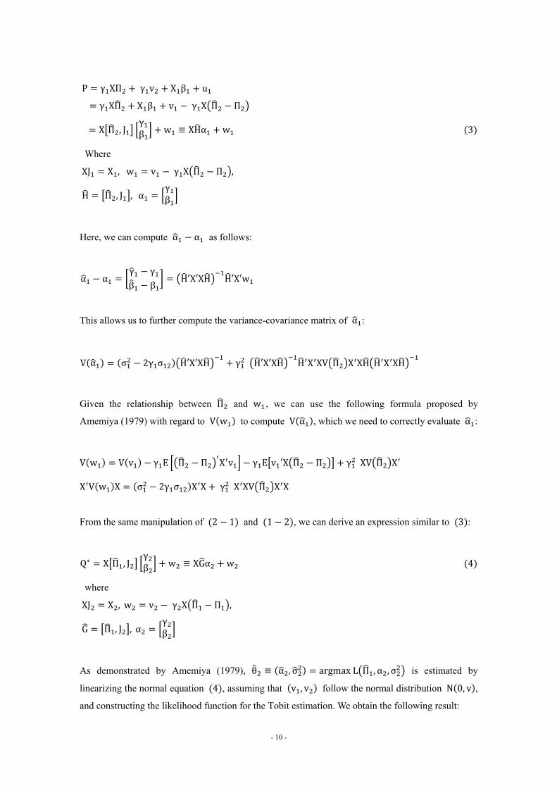
- 10 -

P γ XΠ γ v X β u

γ XΠ X β v γ X Π Π

X Π , Jγβ w ≡ XHα w 3

Where

XJ X ,w v γ X Π Π ,

H Π , J , αγβ

Here, we can compute α α as follows:

α αγ γβ β

H′X′XH H′X′w

This allows us to further compute the variance-covariance matrix of α :

V α σ 2γ σ H′X′XH γ H′X′XH H X XV Π X XH H X XH

Given the relationship between Π and w , we can use the following formula proposed by

Amemiya (1979) with regard to V w to compute V α , which we need to correctly evaluate α :

V w V v γ E Π Π X v γ E v ′X Π Π γ XV Π X

X V w X σ 2γ σ X X γ X XV Π X X

From the same manipulation of 2 1 and 1 2 , we can derive an expression similar to 3 :

Q∗ X Π , Jγβ w ≡ XGα w 4

where

XJ X , w v γ X Π Π ,

G Π , J , αγβ

As demonstrated by Amemiya (1979), θ ≡ α , σ argmaxL Π , α , σ is estimated by

linearizing the normal equation 4 , assuming that v , v follow the normal distribution N 0, v ,

and constructing the likelihood function for the Tobit estimation. We obtain the following result:

- 11 -

θ θ ≡ασ

ασ E

∂ logL∂θ ∂θ ′

∂logL∂θ

E∂ logL∂θ ∂H ′

∙ Π Π

where

Π Π X′X X′v

meansbothsidesoftheequationhavethesameasymptoticdistribution.

Given that the following relationship holds, we can compute V α :

Πσ

G 00′ 1

ασ

V α G V Π G

γ σ 2γ σ G V Π G G V Π X′X V Π G G V Π G

In this context, it is worth noting that the instrumental variable Tobit model proposed by

Smith and Blundell (1986) and Newey (1987), which considers the following limited information

simultaneous equations system with one structural equation (i.e., one endogenous variable) in

5 1 and 5 2 , produces the same estimators, but the standard errors are different:

P γ Q∗ X β u 5 1

Q∗ X Π X Π v 5 2

In the next section, we present the estimated coefficients of the simultaneous equation system

constructed above, for which statistical inference is made by using the variance-covariance matrix

computed as above. We also show the results for the model represented by 5 1 and 5 2

for comparison.

5. Estimation Results

5.1. Baseline Estimation Results

The baseline results of our empirical analysis are presented in Table 3. The columns on the

left show the results for the first-stage regression, while those on the right show those for the

second-stage regression. The first-stage estimation regressing CLN_ISSUE_Q on all the exogenous

variables is provided in the upper part on the left-hand side. The results of this estimation are used to

estimate the seller curve in the second stage, which is shown in the upper part on the right. Similarly,

- 12 -

the first-stage estimation regressing iTraxx_P on all the exogenous variables is presented in the

lower part on the left-hand side and the results are used to estimate the buyer curve in the second

stage. The results are shown in the lower part on the right-hand side. For the second-stage regression,

both standard errors based on the variance-covariance matrix computed as in Amemiya (1979) and

non-corrected standard errors used for the model represented by 5 1 and 5 2 are shown.

The non-corrected standard errors underestimate the true standard errors because they do not reflect

the errors from the first-stage estimation.

Let us take a look at the results. First, the upper and lower parts on the right-hand side

show that the protection seller curve has a significant positive slope (1.5175), while the protection

buyer curve has a significant negative slope (-1/0.5482), which is consistent with our conjecture.15

Second, the protection seller curve shifts down (i.e., protection sellers are willing to sell more

protection at the same premium as before) when general economic conditions improve (i.e.,

NKY_AVG is higher). Third, as the yield on Japanese government bonds decreases (i.e., JGB_5Y

falls), protection sellers attempt to sell more protection. The latter result implies that Japanese

government bonds are an alternative investment asset to CLNs. Fourth, such a downward shift of the

protection seller curve can be also observed when opportunities for loan investments by banks

decrease (LOAN_DEPOST falls). When banks find it difficult to invest the deposits they take into

traditional loan assets, they tend to use the funds to buy, for example, CLNs, as discussed above.

Fifth, protection sellers also tend to sell more protection when the risk of CLN portfolios is lower

(i.e., RATING_CHANGE is lower).

The lower part of the second-stage estimation represents the estimated protection buyer

curve. The negative-sloping buyer curve shifts upward when the speculative motive becomes

stronger (i.e., LIBOR_TREASUR3M increases) and/or the short-cover motive becomes more

significant (i.e., MARK_TO_MKT decreases).

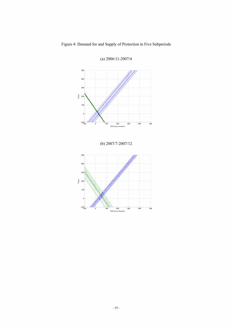
Figure 4 depicts the protection seller and buyer curves for five sub-periods using the

estimated coefficients from Table 3 and the values for the exogenous variables for the five

sub-periods. As can be seeing in panels (a) and (b) of Figure 4, the two curves intersect at relatively

low levels of iTraxx_P – below 100 basis points – during the early part of our observation period.

The intersection shifts up somewhat in the run-up to the collapse of Lehman Brothers in September

2008 (Figure 4(c)) and then jumps to 300 basis points and more in the wake of the collapse of

Lehman Brothers (Figure 4 (d)). Interestingly, the price dynamics prior to the collapse of Lehman

Brothers are mainly driven by a shift in the protection seller curve. On the other hand, shifts in both

the protection seller and buyer curves led to the sharp rise in iTraxx_P after the Lehman collapse,

which confirms our conjecture that both sides contributed to the sharp rise in CDS premiums.

15 Note that, in this estimation, we set CLN_ISSUE_Q as the dependent variable and, in order to compare these slopes, we need to take the inverse of the estimate.

- 13 -

5.2. Two Sources of Potential Bias

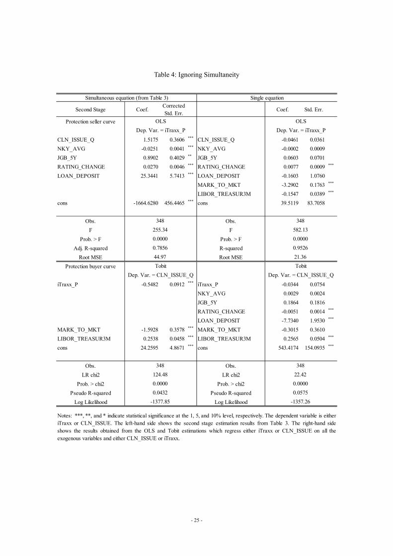
In this subsection, we examine the two potential biases originating from (i) ignoring

simultaneity and (ii) ignoring the limited dependent variable. First, the right-hand side of Table 4

shows the estimated coefficients when we ignore the simultaneous equation system. In this

estimation, the price (quantity) is regressed on the quantity (price) and all other exogenous variables

simply using the OLS (Tobit) specification instead of employing two-stage estimation. The

estimation based on the incorrectly specified iTraxx_P model (i.e., the upper part on the right-hand

side) yields, for example, an insignificant coefficient on LOAN_DEPOSIT. The impact of the two

variables NKY_AVG and JGB5Y, which was found to be significant in the baseline estimation, also

becomes insignificant in this estimation. These results mean that it is necessary to consider both

demand and supply to examine the determinants of CDS premiums.

Second, to investigate the role of another source of bias, namely that resulting from

ignoring the limited dependent variable, we implement linear instrumental variable estimations for

iTraxx_P and CLN_ISSUE_Q, the results of which are shown in Table 5. Given that the purpose of

this exercise is to examine the bias associated with ignoring that CLN_ISSUE_Q is truncated, the

estimation is implemented using regular two-stage least square estimation instead of the model in

1 1 and 1 2 . The results indicate that the signs of the coefficients are consistent with those

of the baseline estimation. To investigate whether the economic impact of each of the exogenous

variables is similar in the two estimations, we compute the change in the predicted value of iTraxx_P

when each variable increases by one standard deviation. The results are shown in Table 6.16 The

column labeled “Baseline” shows the results for the baseline estimation, while that labeled “Ignoring

LDV” shows those when ignoring that CLN_ISSUE_Q is truncated. The impacts of the shift

variables for the protection seller curve (i.e., NKY_AVG, JGB5Y, RATING_CHANGE, and

LOAN_DEPOST) are almost twice as high in the case of the incorrectly specified model. This

implies that we would overestimate the impact of these variables if we do not correctly take into

account the truncation of CLN_ISSUE_Q.

As another comparison between the correctly and incorrectly specified models, the center

column in Table 6 also shows the computed magnitude of each covariate in the estimation of the

“single” equation, which ignores the simultaneity. The fact that the loan-to-deposit ratio is not

significant in the incorrectly specified single equation model suggests that the quantitative impact of

a change in the loan-to-deposit ratio would be measured incorrectly if we do not take the

simultaneous equation system into account. Figures 5 and 6 compare the observed price and quantity

dynamics with the model prediction. The figures show that our model predicts the price and quantity

dynamics reasonably well.

16 The results in Table 6 are obtained by solving the simultaneous equation system.

- 14 -

6. Conclusion

This paper examined the determinants of CDS premiums by employing a simultaneous

equation system consisting of the demand for and supply of protection. The results suggest that CDS

premiums rise when the protection supply curve shifts upward, which may occur when investors’

risk-taking capacity decreases, the returns on alternative investment assets increases, average credit

ratings of existing CLNs in the market deteriorate, and/or business opportunities in commercial

banks’ main business improve; CDS premiums also rise when the protection demand curve shifts

upward, which may occur when the speculative motive and/or the short-cover motive become

stronger. The analysis also showed, however, that the quantitative impact of these factors would be

misestimated unless the simultaneous determination of supply and demand as well as the limited

dependent variable are taken into account. These results mean that, to understand fluctuations in

CDS premiums, it is necessary to explicitly consider demand and supply factors just as in the case of

prices of other financial assets, as well as the truncated data on transaction quantities.

The research presented in this study could be expanded in a number of directions. One

such direction would be to extend our analysis to the determinants of single name CDS spreads

through a panel estimation framework. In order to measure the outright demand for protection with

regard to exposure to individual firms, however, we need to collect more comprehensive transaction

data. Second, a further, potentially interesting extension would be to apply the model in this paper to

explicitly analyze the determinants of the spreads of corporate bonds. Third, an important remaining

issue would be to analyze transactions among market makers, which in this paper are assumed to

play a neutral role. We believe all of these extensions would provide further insights to gain a better

understanding of pricing in the CDS market.

- 15 -

References

Amemiya, T., 1979. The Estimation of a Simultaneous Equation Tobit Model. International

Economic Review 20, 169–181.

Blanco, R., Brennan, S., Marsh, I. W., 2005. An Empirical Analysis of the Dynamic Relation

Between Investment-Grade Bonds and Credit Default Swaps. Journal of Finance 60,

2255–2281.

Bollen, N. P., Whaley, R. E., 2004. Does Net Buying Pressure Affect the Shape of Implied Volatility

Functions? Journal of Finance 59, 711–754.

Brunnermeier, M. K., Pedersen, L. H., 2009. Market Liquidity and Funding Liquidity. Review of

Financial Studies 22, 2201–2238.

Chordia, T., Roll, R., Subrahmanyam, A., 2002. Order Imbalance, Liquidity, and Market Returns.

Journal of Financial Economics 65, 111–130.

Chordia, T., Subrahmanyam, A., 2004. Order Imbalance and Individual Stock Returns: Theory and

Evidence. Journal of Financial Economics 72, 485–518.

Coval, J.A., Stafford, E., 2007. Asset Fire Sales (and Purchases) in Equity Markets. Journal of

Financial Economics 86, 479–512.

Ellul, A., Jotikasthira, P., Lundblad, C. T., 2011. Regulatory Pressure and Fire Sales in the Corporate

Bond Market. Journal of Financial Economics 101, 596–620.

Ericsson, J., Jacobs, K., Oviedo, R. A., 2009. The Determinants of Credit Default Swap Premia.

Journal of Financial and Quantitative Analysis 44, 109–132.

Garleanu, N., Pedersen, L. H., Poteshman, A. M., 2009. Demand-Based Option Pricing, Review of

Financial Studies 22, 4259–4299.

Greenwood, R., Vayanos, D., 2010. Price Pressure in the Government Bond Market. American

Economic Review Papers & Proceedings 100, 585–590.

Hendershott, T., Menkveld, A. J., 2012. Price Pressures. Working Paper.

Huang, Y., Neftci, S., Jersey, I., 2003. What Drives Swap Spreads, Credit or Liquidity? ISMA Centre

Discussion Papers in Finance 2003-2005, University of Reading.

Keshk, O. M. G., 2003. CDSIMEQ: A Program to Implement Two-Stage Probit Least Squares. The

Stata Journal 3, 157–167.

Kraus, A., Stoll, H. R., 1972. Price Impacts of Block Trading on the New York Stock Exchange.

Journal of Finance 27, 569–588.

Krishnamurthy, A., Vissing-Jorgenson, A., 2012. The Aggregate Demand for Treasury Debt. Journal

of Political Economy 120, 233–267.

Longstaff, F., Mithal, S., Neis, E., 2005. Corporate Yield Spreads: Default Risk or Liquidity? New

Evidence from the Credit Default Swap Market. Journal of Finance 60, 2213–2253.

- 16 -

Nelson, F., Olson, L., 1978. Specification and Estimation of a Simultaneous Equation Model with

Limited Dependent Variables. International Economic Review 19, 695–705.

Newey, W. K., 1987. Efficient Estimation of Limited Dependent Variable Models with Endogenous

Explanatory Variables. Journal of Econometrics 36, 231–250.

Sarkar, A., Schwartz, R.A., 2009. Market Sidedness: Insights into Motives for Trade Initiation.

Journal of Finance 64, 375–423.

Scheicher, M., 2008. How Has CDO Market Pricing Changed During the Turmoil? Evidence from

CDS Index Tranches. European Central Bank Working Paper Series No. 910.

Smith, R. J., Blundell, R. W., 1986. An Exogeneity Test for a Simultaneous Equation Tobit Model

with an Application to Labor Supply. Econometrica 54, 679–685.

Tang, D. Y., Yan, H., 2011. What Moves CDS Spreads? Working Paper.

- 17 -

Figure 1: CDS Market

Outright Protection Sellers(Provide Protection &

Receive Premium)

Outright Protection Buyers(Receive Protection &

Pay Premium)

MM

MM

MM

MM

MM

MM

CDS Market (MM: Market Maker)

- 18 -

Figure 2: CDS and CLN Markets

Figure 3: Protection Seller and Buyer Functions

Note: The figure shows the protection selling and buying curves at t=0 (e.g., prior to an event) and t=1 (after the

event).

Premium PaymentCLN Coupon Payment

= CDS Premium payment

Buy CLN

= Sell protection (through CDS)

Sell Protection

OutrightProtection

Sellers

SecuritiesFirms

OutrightProtection

Buyers

CLN Market CDS Market

Q: CDS Transaction Volume

Seller sells protection & Buyer buys protection

Seller (t=0)

Buyer (t=0)

Buyer (t=1)

Seller (t=1)

P: CDS Premium

- 19 -

Figure 4: Demand for and Supply of Protection in Five Subperiods

(a) 2006/11-2007/4

(b) 2007/7-2007/12

-100 0 100 200 300 400 500-100

0

100

200

300

400

500

CLN Issue Amount

iTra

xx

-100 0 100 200 300 400 500-100

0

100

200

300

400

500

CLN Issue Amount

iTra

xx

- 20 -

Figure 4 (continued): Demand for and Supply of Protection in Five Subperiods

(c) 2008/2-2008/7

(d) 2008/10-2009/3

(e) 2010/3-2010/8

Note: Each figure plots the protection selling and buying curves based on the estimated results. The intersections of

the two curves are obtained by solving the simultaneous equation system.

-100 0 100 200 300 400 500-100

0

100

200

300

400

500

CLN Issue Amount

iTra

xx

-100 0 100 200 300 400 500-100

0

100

200

300

400

500

CLN Issue Amount

iTra

xx

-100 0 100 200 300 400 500-100

0

100

200

300

400

500

CLN Issue Amount

iTra

xx

- 21 -

Figure 5: Predicted Price

Note: P stands for the actually observed iTraxx Japan, while Predicted P is the model prediction. Each point is

obtained by solving the estimated simultaneous equation system.

Figure 6: Predicted Quantity

Note: Q stands for the actually observed CLN issuance volume, while Predicted Q is the model prediction. Each point

is obtained by solving the estimated simultaneous equation system.

-100

0

100

200

300

400

500

600

2004/08/06 2005/08/06 2006/08/06 2007/08/06 2008/08/06 2009/08/06 2010/08/06

Bas

is P

oint

s

P

Predicted P

-50

0

50

100

150

200

250

2004/08/06 2005/08/06 2006/08/06 2007/08/06 2008/08/06 2009/08/06 2010/08/06

Bas

is P

oint

s

Q

Predicted Q

- 22 -

Table 1: Summary Statistics

Variable Definition Unit Obs. Mean Std. Dev. Min. Max.

iTraxx_P Markit iTraxx Japan bp 348 93.37 97.13 16.26 552.94

CLN_ISSUE_Q Issued CLN amount100 million

yen348 22.72 35.63 0.00 214.00

NKY_AVGMonthly average of Nikkei 225Stock Index

yen 348 12629 3012 7257 18191

JGB_5YYield of 5-year Japanesegovernment bonds

bp 348 84 33 23 154

RATING_CHANGE

Issued amount of each CLN timesthe concurrent change in its ratings(1 if downgraded and -1 ifupgraded)

- 348 2113 2756 -23 6993

LOAN_DEPOSIT Loan to deposit ratio % 348 75.68 1.74 70.43 78.29

MARK_TO_MKTPotential gains (positive number)and losses (negative number) fromCLNs investment

- 348 -17.57 26.85 -117.55 6.14

LIBOR_TREASUR3M3-month Libor minus yield on 3-month US treasuries

bp 348 58.95 60.03 9.99 410.93

Note: The table shows the summary statistics for the variables used in the estimation. Our observation period is

from August 2004 to April 2011, providing 348 weekly observations for each of the variables.

- 23 -

Table 2: Correlation Coefficients

(Obs.=348)

(1) (2) (3) (4) (5) (6) (7) (8)

(1) iTraxx_P 1.00

(2) CLN_ISSUE_Q -0.14 1.00

(3) NKY_AVG -0.68 0.38 1.00

(4) JGB_5Y -0.25 0.46 0.80 1.00

(5) RATING_CHANGE 0.58 -0.38 -0.73 -0.63 1.00

(6) LOAN_DEPOSIT -0.07 0.15 0.36 0.52 -0.68 1.00

(7) MARK_TO_MKT -0.94 0.01 0.57 0.10 -0.38 -0.11 -0.54

(8) LIBOR_TREASUR3M 0.37 0.43 -0.04 0.30 -0.13 0.24 1.00 1.00

Note: The table shows the correlation coefficients for the variables used for the estimation. Our observation period is

from August 2004 to April 2011, providing 348 weekly observations for each of the variables.

- 24 -

Table 3: Baseline Results

First Stage Coef. Std. Err. Second Stage Coef.CorrectedStd. Err.

Non-CorrectedStd. Err.

Protection seller curve Protection seller curve

CLN_ISSUE_Q CLN_ISSUE_Q 1.5175 0.3606 *** 0.1678 ***

NKY_AVG 0.0029 0.0019 NKY_AVG -0.0251 0.0041 *** 0.0019 ***

JGB_5Y 0.1852 0.1376 JGB_5Y 0.8902 0.4029 ** 0.1872 ***

RATING_CHANGE -0.0054 0.0015 *** RATING_CHANGE 0.0270 0.0046 *** 0.0021 ***

LOAN_DEPOSIT -7.7658 1.8255 *** LOAN_DEPOSIT 25.3441 5.7413 *** 2.6580 ***

MARK_TO_MKT -0.1872 0.1411

LIBOR_TREASUR3M 0.2626 0.0417 ***

cons 544.9784 143.5038 *** cons -1664.6280 456.4465 *** 211.2360 ***

Obs. Obs.

LR chi2 F

Prob. > chi2 Prob. > F

Pseudo R-squared Adj. R-squared

Log Likelihood Root MSE

Protection buyer curve Protection buyer curve

iTraxx_P iTraxx_P -0.5482 0.0912 *** 0.1154 ***

NKY_AVG -0.0003 0.0012

JGB_5Y 0.0515 0.0860

RATING_CHANGE 0.0079 0.0009 ***

LOAN_DEPOSIT 0.1640 1.1384

MARK_TO_MKT -3.2859 0.0889 *** MARK_TO_MKT -1.5928 0.3578 *** 0.4457 ***

LIBOR_TREASUR3M -0.1650 0.0266 *** LIBOR_TREASUR3M 0.2538 0.0458 *** 0.0530 ***

cons 15.8964 89.3725 cons 24.2595 4.8671 *** 5.8669 ***

Obs. Obs.

F LR chi2

Prob. > F Prob. > chi2

Adj. R-squared Pseudo R-squared

Root MSE Log Likelihood

Notes: ***, **, and * indicate statistical significance at the 1, 5, and 10% level, respectively. The dependent variable is either iTraxx orCLN_ISSUE. The left-hand side shows the results of the first-stage reduced form regression. The right-hand side shows the second stageregressions for the protection seller and buyer functions. The column "Corrected Std. Err." shows the standard error adjusted following themethodology employed by Nelson & Olson (1978) and refined by Amemiya (1979), while the column "Non-Corrected Std. Err." shows theunadjusted standard error.

348

255.34

0.0000

0.7856

44.97

348

0.9516

21.37

0.0432

-1377.85

1138.03

0.0000

124.48

0.0000

OLS

Dep. Var. = iTraxx_P Dep. Var. = CLN_ISSUE_Q

348

Tobit

0.0575

-1357.34

Simultaneous equation

165.51

0.0000

Tobit

Dep. Var. = CLN_ISSUE_Q Dep. Var. = iTraxx_P

348

OLS

- 25 -

Table 4: Ignoring Simultaneity

Second Stage Coef.CorrectedStd. Err.

Coef. Std. Err.

Protection seller curve

CLN_ISSUE_Q 1.5175 0.3606 *** CLN_ISSUE_Q -0.0461 0.0361

NKY_AVG -0.0251 0.0041 *** NKY_AVG -0.0002 0.0009

JGB_5Y 0.8902 0.4029 ** JGB_5Y 0.0603 0.0701

RATING_CHANGE 0.0270 0.0046 *** RATING_CHANGE 0.0077 0.0009 ***

LOAN_DEPOSIT 25.3441 5.7413 *** LOAN_DEPOSIT -0.1603 1.0760

MARK_TO_MKT -3.2902 0.1763 ***

LIBOR_TREASUR3M -0.1547 0.0389 ***

cons -1664.6280 456.4465 *** cons 39.5119 83.7058

Obs. Obs.

F F

Prob. > F Prob. > F

Adj. R-squared R-squared

Root MSE Root MSE

Protection buyer curve

iTraxx_P -0.5482 0.0912 *** iTraxx_P -0.0344 0.0754

NKY_AVG 0.0029 0.0024

JGB_5Y 0.1864 0.1816

RATING_CHANGE -0.0051 0.0014 ***

LOAN_DEPOSIT -7.7340 1.9530 ***

MARK_TO_MKT -1.5928 0.3578 *** MARK_TO_MKT -0.3015 0.3610

LIBOR_TREASUR3M 0.2538 0.0458 *** LIBOR_TREASUR3M 0.2565 0.0504 ***

cons 24.2595 4.8671 *** cons 543.4174 154.0935 ***

Obs. Obs.

LR chi2 LR chi2

Prob. > chi2 Prob. > chi2

Pseudo R-squared Pseudo R-squared

Log Likelihood Log Likelihood

0.0000

0.0575

-1357.26

Simultaneous equation (from Table 3) Single equation

0.9526

21.36

Tobit

Dep. Var. = CLN_ISSUE_Q

348

22.42

0.0432

-1377.85

Dep. Var. = iTraxx_P

348

Notes: ***, **, and * indicate statistical significance at the 1, 5, and 10% level, respectively. The dependent variable is eitheriTraxx or CLN_ISSUE. The left-hand side shows the second stage estimation results from Table 3. The right-hand sideshows the results obtained from the OLS and Tobit estimations which regress either iTraxx or CLN_ISSUE on all theexogenous variables and either CLN_ISSUE or iTraxx.

OLS

Dep. Var. = iTraxx_P

348

582.13

0.0000

348

124.48

0.0000

44.97

Tobit

Dep. Var. = CLN_ISSUE_Q

255.34

0.0000

0.7856

OLS

- 26 -

Table 5: Ignoring the Limited Dependent Variable

Second Stage Coef.CorrectedStd. Err.

Second Stage Coef. Std. Err.

Protection seller curve Protection seller curve

CLN_ISSUE_Q 1.5175 0.3606 *** CLN_ISSUE_Q 1.6407 0.3754 ***

NKY_AVG -0.0251 0.0041 *** NKY_AVG -0.0256 0.0036 ***

JGB_5Y 0.8902 0.4029 ** JGB_5Y 1.0014 0.3471 ***

RATING_CHANGE 0.0270 0.0046 *** RATING_CHANGE 0.0266 0.0033 ***

LOAN_DEPOSIT 25.3441 5.7413 *** LOAN_DEPOSIT 25.4084 4.4336 ***

cons -1664.6280 456.4465 *** cons -1683.7840 350.7460 ***

Obs. Obs.

F F

Prob. > F Prob. > F

Adj. R-squared R-squared

Root MSE Root MSE

Protection buyer curve Protection buyer curve

iTraxx_P -0.5482 0.0912 *** iTraxx_P -0.3971 0.0790 ***

MARK_TO_MKT -1.5928 0.3578 *** MARK_TO_MKT -1.0673 0.3337 ***

LIBOR_TREASUR3M 0.2538 0.0458 *** LIBOR_TREASUR3M 0.2317 0.0632 ***

cons 24.2595 4.8671 *** cons 27.3863 5.3824 ***

Obs. Obs.

LR chi2 F

Prob. > chi2 Prob. > F

Pseudo R-squared R-squared

Log Likelihood Root MSE

Notes: ***, **, and * indicate statistical significance at the 1, 5, and 10% level, respectively. The dependent variable is eitheriTraxx or CLN_ISSUE. The left-hand side shows the second stage estimation results from Table 3. The right-hand sideshows the results obtained from the two IV estimations without considering the limited dependent variable (i.e.,CLN ISSUE Q) in the estimation.

0.0000 0.0000

0.0432 0.2691

-1377.85 30.59

Dep. Var. = CLN_ISSUE_Q Dep. Var. = CLN_ISSUE_Q

348 348

124.48 50.61

0.7856 0.5420

44.97 66.21

Tobit OLS

348 348

255.34 91.42

0.0000 0.0000

Simultaneous equationconsidering LDV (from Table 3)

Simultaneous equationwithout considering LDV

OLS OLS

Dep. Var. = iTraxx_P Dep. Var. = iTraxx_P

- 27 -

Table 6: Comparison of Economic Impacts

BaselineSingle

equationIgnoring

LDV

Δ1 std. dev. ↑ in NKY_AVG -24.6 0.0 -46.7

JGB_5Y 9.7 0.0 20.3

RATING_CHANGE 24.3 21.3 44.4

LOAN_DEPOSIT 14.4 0.0 26.8

MARK_TO_MKT -21.2 -88.4 -15.5

LIBOR_TREASUR3M 7.5 -9.3 7.5

Predicted change in iTraxx_P(bp)

Change in Exogenous Variable

Note: The column "Baseline" shows the predicted change in iTraxx_P in the case that eachcovariate increases by one standard deviation. The results are based on the estimated parameters inTable 3. The next two columns show the results of the same exercise based on the estimatedparameters in Tables 4 and 5, respectively. All changes in iTraxx_P are measured in terms of bp.