Water Resources Research Report - Western University · The ANSYS tools that can be accessed from...

THE UNIVERSITY OF WESTERN ONTARIO

DEPARTMENT OF CIVIL AND

ENVIRONMENTAL ENGINEERING

Water Resources Research Report

Report No: 098

Date: October 2017

General Methodology for Developing a CFD Model

for Studying Spillway Hydraulics using ANSYS

Fluent

By:

R Arunkumar

and

Slobodan P. Simonovic

ISSN: (print) 1913-3200; (online) 1913-3219

ISBN: (print) 978-0-7714-3148-7; (online) 978-0-7714-3149-4

i

General Methodology for Developing a CFD Model for

Studying Spillway Hydraulics using ANSYS Fluent

R. Arunkumar

&

Slobodan P. Simonovic

Department of Civil and Environmental Engineering

The University of Western Ontario

London - N6A 5B9, Ontario, Canada

ii

Executive Summary

The advancement of computing facilities has led to the development of advanced software

packages and tools for solving various practical engineering problems. One such advancement is

the development of various computational fluid dynamic (CFD) software with different numerical

solver methods. These computational methods are identified as suitable tools for solving various

engineering problems. They also have various advantages over the traditional physical modeling.

One such CFD software tool is ANSYS Fluent. In this report, the general guide and practical steps

for developing a full 3D CFD spillway model using ANSYS Fluent have been presented.

iii

Table of Contents

Executive Summary ii

Table of Contents iii

List of Figures iv

1. Introduction 1

2. ANSYS Fluent 2

2.1. General Methodology for Developing a CFD Model 3

2.2. Developing an ANSYS Workbench Project 4

2.3. Creating / Importing Geometry 5

2.4. Mesh Generation 8

2.5. Model Development in ANSYS Fluent 14

2.5.1 General Setting 16

2.5.2 Model Selection 17

2.5.3 Materials 19

2.5.4 Cell Zone Condition 20

2.5.5 Boundary Conditions 21

2.5.6 Solution Methods 24

2.5.7 Solution Control 24

2.5.8 Monitors 25

2.5.9 Solution Initialization 26

2.5.10 Run Calculation 28

2.6. Results and Post Processing 29

3. Summary 29

Acknowledgments 29

References 29

Appendix A: List of Previous Reports in the Series 31

iv

List of Figures

Figure 1. General methodology ...................................................................................................... 4

Figure 2 ANSYS workbench and its various tools ......................................................................... 5

Figure 3. ANSYS toolbox ............................................................................................................... 6

Figure 4. Invoking ANSYS-DesignModeler .................................................................................. 7

Figure 5. ANSYS Design Modeller ................................................................................................ 7

Figure 6. Workflow update - I ....................................................................................................... 8

Figure 7. Interface of ANSYS Meshing tool .................................................................................. 9

Figure 8. ANSYS Meshing tool ...................................................................................................... 9

Figure 9. Various mesh settings .................................................................................................... 10

Figure 10. Creating ‘nameports’ .................................................................................................. 11

Figure 11. View of sample ‘nameports’ in ANSYS Meshing tool .............................................. 11

Figure 12. Progress of mesh creation ............................................................................................ 12

Figure 13. A fully developed mesh using ANSYS-Meshing tool ................................................ 12

Figure 14. Mesh quality matrices.................................................................................................. 13

Figure 15. Number of mesh elements ........................................................................................... 13

Figure 16. Workflow update - II ................................................................................................... 13

Figure 17. ANSYS Fluent launch screen ...................................................................................... 14

Figure 18. ANSYS Fluent main interface ..................................................................................... 15

Figure 19. Steps involved in setting up the ANSYS Fluent model .............................................. 15

Figure 20. General model setting in the ANSYS Fluent tool ....................................................... 16

Figure 21 Selection of VOF model ............................................................................................... 17

Figure 22. Selecting the turbulence model ................................................................................... 18

Figure 23. Selection of materials .................................................................................................. 19

Figure 24. Defining phases and their interactions ........................................................................ 20

Figure 25. Setting up operating conditions ................................................................................... 21

Figure 26 Defining boundary conditions in ANSYS Fluent ......................................................... 22

Figure 27. Pressure inlet boundary conditions .............................................................................. 23

Figure 28. Wall boundary conditions............................................................................................ 23

Figure 29. Different solution methods .......................................................................................... 24

Figure 30. Setting various simulation parameters......................................................................... 25

Figure 31. Monitor control ............................................................................................................ 26

Figure 32. Solution initialization .................................................................................................. 26

Figure 33. Creating specific cell zones and cell adaptation characteristics .................................. 27

Figure 34. Region adaptation and patching .................................................................................. 28

Figure 35 Run calculation ............................................................................................................. 28

1

1. Introduction

The spillway is an important hydraulic structure of a dam, which facilitates the safe passage of

flow from the upstream reservoir to the downstream. A hydraulically efficient and structurally

strong spillway is very important for the dam safety, and protection of the life and property at the

downstream. Many hydraulic models have been extensively developed to study, visualize and

understand the hydraulic behavior of flow over the spillway. Various hydraulic design aspects such

as discharge capacity, velocity, pressure and water surface profiles are considered to study the

spillway hydraulics. The hydraulic behavior of flow over spillway can be studied through physical

or numerical modeling. Physical modeling of spillways is expensive, cumbersome and time

consuming (Savage and Johnson, 2001). To overcome the limitations of the physical modeling,

numerical models including three-dimensional (3D) computational fluid dynamics (CFD) tools

have been used in recent years due to the advancement in computing technology and numerical

methods.

A diverse variety of problems can be studied using CFD modeling. It is widely used in fluid

mechanics, aerodynamics, multiphase, and free-surface flow studies, etc. In dam engineering,

CFD modeling have been widely used to study the hydraulic performance of various types of

spillways, eg. ogee spillway (Savage and Johnson, 2001), circular spillway (Rahimzadeh et al.,

2012), stepped spillway (Chanel and Doering, 2008; Chinnarasri et al., 2014; Dursun and Ozturk,

2016), and also for labyrinth weirs (Savage et al., 2016), rectangular channels (Mohsin and

Kaushal, 2016) and many more. Aydin and Ozturk (2009) reported that the CFD models are more

flexible and require less time, money, and effort than physical hydraulic models. The other

advantage of CFD modeling is that the scale effects of physical modeling can also be eliminated

2

through the real dimensions of the prototype developed using in the CFD model (Bhajantri et al.,

2006). All these studies reported that the CFD is a reliable method for assessing the hydraulic

characteristics of a spillway. However, these studies also cautioned that CFD cannot be a complete

replacement for physical modeling, but it can definitely be used as a supplementary tool for the

spillway design process (Chanel and Doering, 2008). There are many CFD software packages

available, both including open source and preoperatory software. OPENFOAM is an open sources

CFD software package (OpenFOAM, 2017). The other proprietary software packages include

ANSYS Fluent, FLOW-3D, and others. This report focuses on the methodology of developing a

3D CFD spillway model using the ANSYS Fluent (ANSYS, 2016).

The report is organized in the following manner. The general introduction to ANSYS is given in

Section 2. The four major steps involved in developing a CFD model is discussed in Section 2.1.

The step by step procedure in developing an ANSYS Workbench Project is discussed in Section

2.2. The process of creating the geometry of the structure is given in Section 2.3. The steps

involved in creating mesh is discussed in Section 2.4. The full model development using ANSYS

Fluent is discussed in detail in Section 2.5. The analysis of results is given in Section 2.6.

2. ANSYS Fluent

Computational fluid dynamic software package ANSYS Fluent (ANSYS, 2016) is extensively

used to develop 2-D and 3-D models for the fluid flow simulation. It is a state of the art computer

program for modelling fluid flow in complex geometries. All functions required to compute a

solution and display the results are available in ANSYS Fluent through an interactive menu driven

interface. The software package includes ANSYS Fluent solver, pre-processor tool for geometry

3

modelling and mesh developer. The ANSYS Fluent solver has capability of modelling

incompressible, two phase, and free surface turbulent flows in unsteady mode and therefore it was

found suitable for modelling flow over spillway aerator. ANSYS Fluent’s parallel solver allows

for computation by using multiple processes on the same computer. Parallel ANSYS Fluent splits

up the grid and data into multiple partitions, then assigns each grid partition to a different computer

process. Considering all these features ANSYS Fluent was selected for the spillway simulation

modeling in the present study. The various steps in problem formulation, obtaining the solution

and analyzing the results are described in the following text.

2.1. General Methodology for Developing a CFD Model

There are four basic primary steps involved in developing a 3D CFD model as shown in Figure 1.

The first step is the creation of the structure geometry. ANSYS Fluent have its own geometry

builder. Otherwise, the structure geometry can be created in any computer aided design (CAD)

software and then imported into the ANSYS Fluent module. The second step is creating the mesh.

Meshing is the process of describing the structure using mesh of different shapes and sizes, as

cubes, prism, tetrahedral, hexacore, or hybrid volumes (ANSYS, 2013). For each of these mesh

units, the hydraulic particulars are computed using the numerical method in the ANSYS Fluent.

The developed mesh is then imported into the ANSYS Fluent and the solution is obtained using

different solvers depending on the type of analysis. Finally, the results are analyzed using a

separate graphical analysis tool in ANSYS. Alternatively, the results can also be analyzed within

ANSYS Fluent which offers some limited functionalities.

4

Creation of geometry of the structure

Mesh Development

Fluent Model Development &

Computation

Analysis of the results

Figure 1. General methodology

The detailed procedure involved in developing an ANSYS Fluent workbench model is explained

below.

2.2. Developing an ANSYS Workbench Project

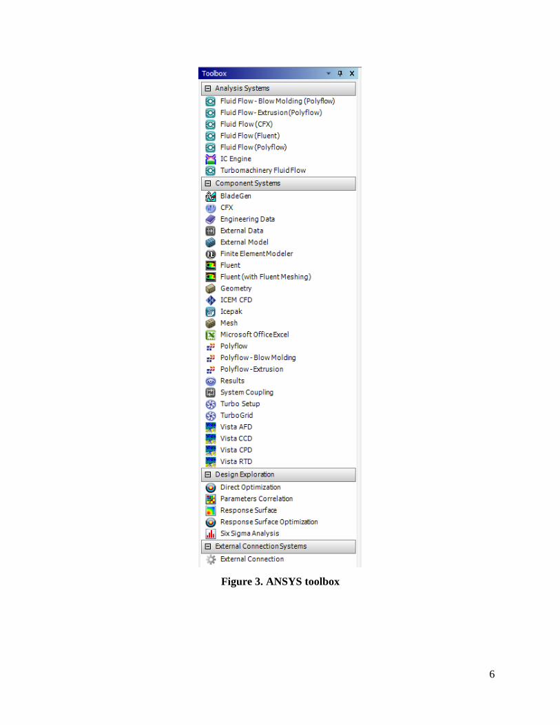
ANSYS Workbench combines access to ANSYS applications with utilities that manage the

product workflow. The ANSYS tools that can be accessed from the workbench are ANSYS

DesignModeler for creating geometry, Meshing tool for generating mesh, Fluent or CFX tool for

setting up and solving fluid dynamics analyses and ANSYS CFD-Post tool for postprocessing the

results. The home screen of workbench is shown in Figure 2. From the ANSYS workbench, the

‘Fluid Flow (ANSYS Fluent)’ has to be drag and dropped into the project window to initiate the

modelling process. Alternatively, one can select each tool (Geometry, Mesh, Fluent, Results)

individually and create a project. The project may be saved with a user defined name in the File

menu.

5

Figure 2 ANSYS workbench and its various tools

The complete ANSYS toolbox is shown in Figure 3.

2.3. Creating / Importing Geometry

The geometry of the structure can be imported from any external design software like AutoCAD

or simply created with ANSYS-Design Modeler. By right clicking on ‘Geometry’ in the ANSYS

workbench project, the ANSYS-Design Modeler can be initiated, as shown in Figure 4. The

interface of ANSYS Design Modeler is shown in Figure 5. Generation of geometry can be carried

out by creating points, edges, faces and volumes of the geometry in three dimensions. After

creating/importing the geometry of the structure into the Design Modeler, the fluid flow regions

(liquid) and solids regions (solid) of the structure have to be defined. The geometry needs to be

divided into separate regions in order to apply constraints for the resulting mesh. Boundary regions

are need to be specified for finer or denser meshing.

6

Figure 3. ANSYS toolbox

7

Figure 4. Invoking ANSYS-DesignModeler

Figure 5. ANSYS Design Modeller

8

When the procedure is correctly done, the workbench tool box will show a green tick mark next

to the ‘Geometry’ as shown in Figure 6. Whenever each step is completed successfully, the green

tick mark will appear on the right side. The process which requires an update or has any error will

be highlighted by different symbols.

Figure 6. Workflow update - I

2.4. Mesh Generation

The Meshing tool can be invoked by right clicking on ‘Mesh’ at the workbench project and

selecting ‘Edit’, similar to ANSYS-Design Modeler. The home interface of ANSYS Meshing tool

is shown in Figure 7. For creating the mesh, the ‘Objects’ have to be identified. An object is

generally a set of face zones and edge zones. Objects are generally closed solid volumes or closed

fluid volumes. Different types of mesh can be created in ANSYS Meshing tool through ‘Insert’

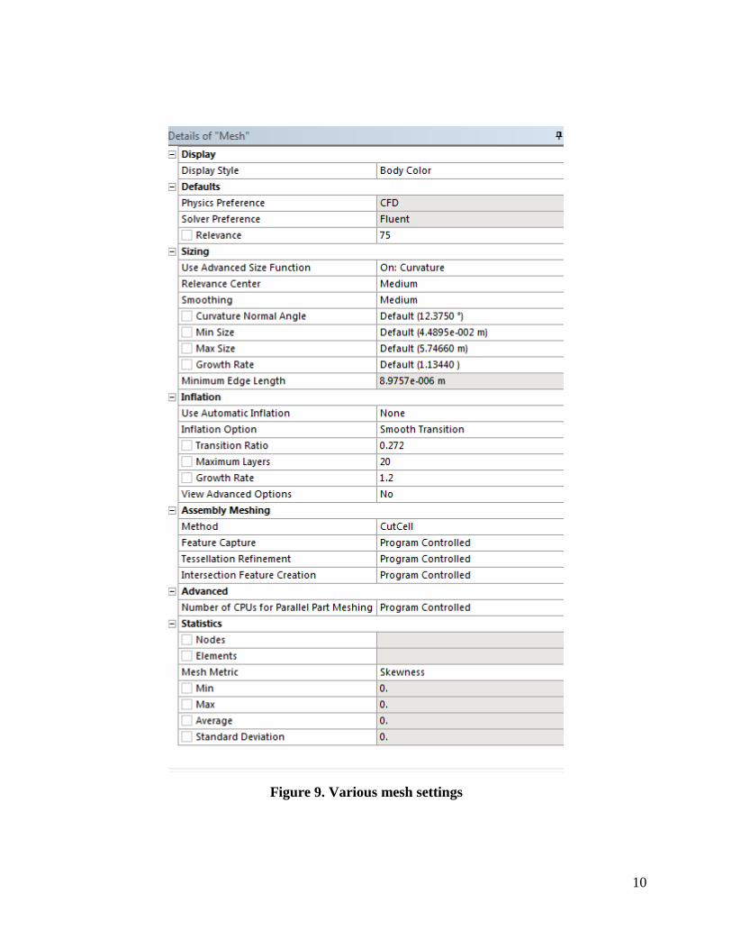
option as shown in Figure 8. The mesh settings can be adjusted according to the model requirement

as seen in Figure 9. After creating the mesh, the proceeds with assigning the ‘nameports’ for

different parts of the model structure. This is helpful for defining the boundary conditions. The

‘nameports’ can be created by right clicking on the region and selecting ‘Create Named Selection’

as shown in Figure 10.

9

Figure 7. Interface of ANSYS Meshing tool

Figure 8. ANSYS Meshing tool

10

Figure 9. Various mesh settings

11

Figure 10. Creating ‘nameports’

Figure 11 shows the sample of various regions that have been defined using ‘nameports’. The

boundary conditions have to be specified in the ANSYS Fluent for all these regions.

Figure 11. View of sample ‘nameports’ in ANSYS Meshing tool

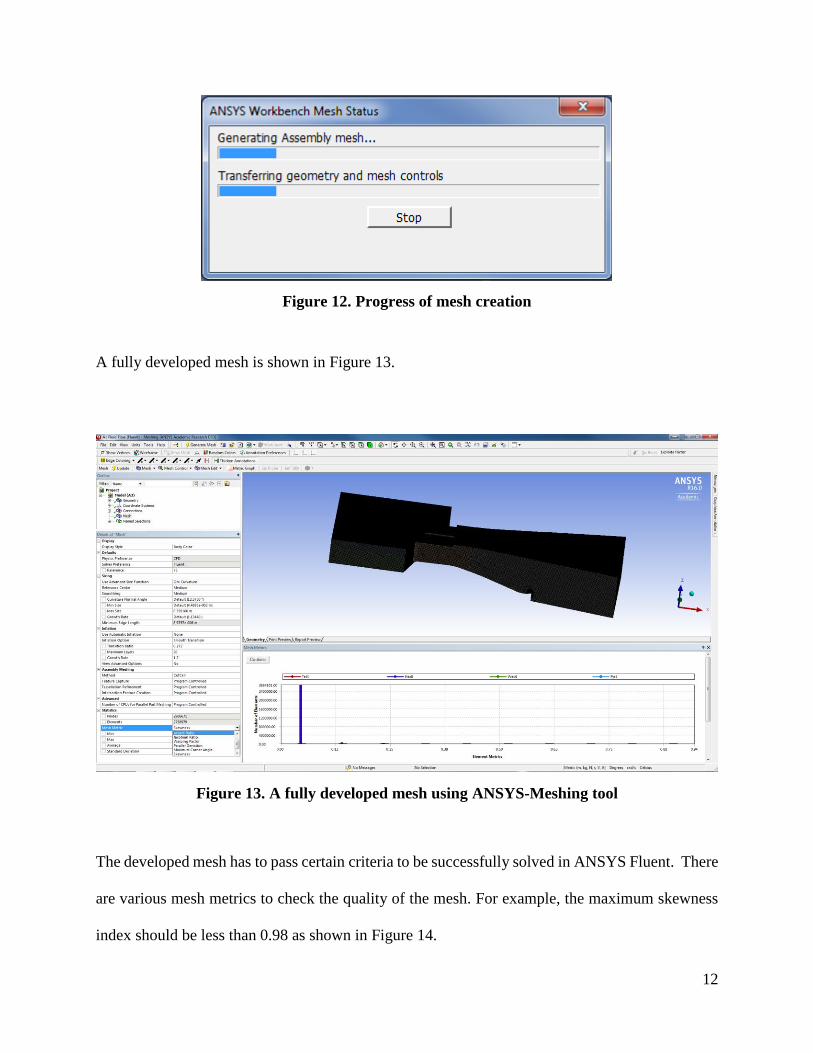
Finally, the mesh can be generated by selecting ‘Generate Mesh’. The status of mesh generation

process is displayed as shown in Figure 12.

12

Figure 12. Progress of mesh creation

A fully developed mesh is shown in Figure 13.

Figure 13. A fully developed mesh using ANSYS-Meshing tool

The developed mesh has to pass certain criteria to be successfully solved in ANSYS Fluent. There

are various mesh metrics to check the quality of the mesh. For example, the maximum skewness

index should be less than 0.98 as shown in Figure 14.

13

Figure 14. Mesh quality matrices

The mesh quality parameters can also be viewed as graphs, as shown in Figure 15.

Figure 15. Number of mesh elements

When the mesh is successfully developed, the ANSYS workbench is updated with the green tick

mark as shown in Figure 16.

Figure 16. Workflow update - II

14

2.5. Model Development in ANSYS Fluent

After the mesh generation, the geometry should be exported as a mesh file for use in ANSYS

Fluent. The ANSYS Fluent can be launched from the workbench either by double clicking or

right clicking and selecting ‘Edit’ in the ‘Setup’ menu. The ANSYS Fluent launch screen is shown

in Figure 17(a). While launching the ANSYS Fluent, the user has to select optional modelling

aspects like 2D or 3D, Double Precision or Meshing modes, Serial or Parallel processing, etc. as

shown in Figure 17(b).

(a)

(b)

Figure 17. ANSYS Fluent launch screen

The main ANSYS Fluent interface is shown in Figure 18.

15

Figure 18. ANSYS Fluent main interface

The steps involved in setting up the ANSYS Fluent model are shown in Figure 19.

Figure 19. Steps involved in setting up the ANSYS Fluent model

16

Each step is explained in detail in the further sections.

2.5.1 General Setting

The options for general model setting in ANSYS Fluent is shown in Figure 20. First, developed

mesh has to be checked in ANSYS Fluent for its quality. Any irregular shapes or sizes have to be

rectified before developing a full model. Only when the parameters such aspect ratio, skewness

index, etc. are within the specified range, the model development in ANSYS Fluent can proceed.

The checks are performed by selecting ‘Check’ and ‘Report Quality’ from the menu screen shown

in Figure 20. The ‘Time’ option is used to select either steady or unsteady state.

Figure 20. General model setting in the ANSYS Fluent tool

17

2.5.2 Model Selection

There are various models available within the ANSYS Fluent. A specific model has to be selected

for the particular problem at hand. For our spillway example, the flow over a spillway involves

two phases, both water and air. Hence, the Multiphase Volume of Fluid model (VOF) has been

selected as shown in Figure 21. It is a multi-phase model best suited for the two phase air-water

flow (ANSYS, 2013). In VOF, each phase is considered as the volume fractions (α1, α2) and the

momentum, heat and mass exchanges are calculated between the phases.

Figure 21 Selection of VOF model

18

An appropriate model has to be selected to consider the turbulent flow over the spillway. There

are various turbulence models available in ANSYS Fluent as shown in Figure 22. In this study,

realizable k-ε model (k-epsilon model) has been selected. The realizable k-ε model is a semi-

empirical model based on model transport equations for the turbulence kinetic energy (k) and its

dissipation rate (ε).

Figure 22. Selecting the turbulence model

19

2.5.3 Materials

After selecting the appropriate model for the problem, the materials involved in problem have to

be defined. ANSYS Fluent has its own database of different “materials” with their properties.

Users can also manually input the material with its properties, if it is not available in the database.

The selection of materials window is shown in Figure 23. As already mentioned, the spillway is

modelled as a multi-phase model and involves both air and water. Hence, air and water materials

are selected from the ANSYS Fluent database.

Figure 23. Selection of materials

20

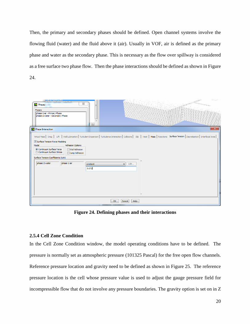
Then, the primary and secondary phases should be defined. Open channel systems involve the

flowing fluid (water) and the fluid above it (air). Usually in VOF, air is defined as the primary

phase and water as the secondary phase. This is necessary as the flow over spillway is considered

as a free surface two phase flow. Then the phase interactions should be defined as shown in Figure

24.

Figure 24. Defining phases and their interactions

2.5.4 Cell Zone Condition

In the Cell Zone Condition window, the model operating conditions have to be defined. The

pressure is normally set as atmospheric pressure (101325 Pascal) for the free open flow channels.

Reference pressure location and gravity need to be defined as shown in Figure 25. The reference

pressure location is the cell whose pressure value is used to adjust the gauge pressure field for

incompressible flow that do not involve any pressure boundaries. The gravity option is set on in Z

21

direction at -9.81 m/s2, which is necessary as the flow over spillway is gravity driven. The negative

sign indicates that the gravity is downwards in the Z direction. The variable density parameter is

set as operating density for the phase air at 1.225 kg/m3.

Figure 25. Setting up operating conditions

2.5.5 Boundary Conditions

The most important aspect of setting up the simulation is the definition of the boundary conditions.

There are various boundary conditions available in ANSYS Fluent. The boundary conditions for

each face/zone have to be selected according to the problem as shown in Figure 26. Basically, the

spillway hydraulics have three types of boundary zones viz. pressure inlet, wall and pressure outlet.

The upstream end of the reservoir is the flow inlet. The velocity of flow is known, then velocity

inlet can be given. For most of the spillway hydraulics problem, the flow velocity is unknown.

Hence, the upstream inlet is defined as a pressure inlet (shown in Figure 27) to maintain a reservoir

water level. The turbulence specification is given as ‘intensity and viscosity ratio’, that requires

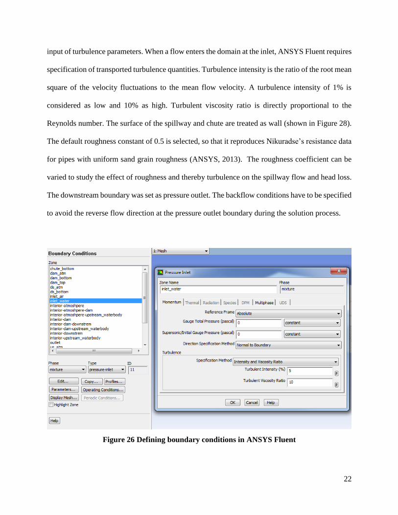
22

input of turbulence parameters. When a flow enters the domain at the inlet, ANSYS Fluent requires

specification of transported turbulence quantities. Turbulence intensity is the ratio of the root mean

square of the velocity fluctuations to the mean flow velocity. A turbulence intensity of 1% is

considered as low and 10% as high. Turbulent viscosity ratio is directly proportional to the

Reynolds number. The surface of the spillway and chute are treated as wall (shown in Figure 28).

The default roughness constant of 0.5 is selected, so that it reproduces Nikuradse’s resistance data

for pipes with uniform sand grain roughness (ANSYS, 2013). The roughness coefficient can be

varied to study the effect of roughness and thereby turbulence on the spillway flow and head loss.

The downstream boundary was set as pressure outlet. The backflow conditions have to be specified

to avoid the reverse flow direction at the pressure outlet boundary during the solution process.

Figure 26 Defining boundary conditions in ANSYS Fluent

23

Figure 27. Pressure inlet boundary conditions

Figure 28. Wall boundary conditions

24

2.5.6 Solution Methods

There are solution methods available in ANSYS Fluent to solve the model as shown in Figure 29.

The solution methods should be selected according to the problem type.

Figure 29. Different solution methods

2.5.7 Solution Control

Sometimes, certain parameter values need to be relaxed for the successful simulation. Those

parameter settings can be adjusted as shown in Figure 30.

25

Figure 30. Setting various simulation parameters

2.5.8 Monitors

During the simulation process, users can monitor and visualize certain parameters which are

significant for the simulation. Those parameters can be set in monitor control window as shown in

Figure 31. The values of the defined parameters will be displayed as graphs in the monitor during

the simulation process.

26

Figure 31. Monitor control Figure 32. Solution initialization

2.5.9 Solution Initialization

Before starting the CFD simulation, ANSYS Fluent needs the initial value for the solution field.

The solution initialization can be done by two ways as shown in Figure 32. First, the initialization

27

is done for the entire flow field. Then, specific regions or zones are created and patch values or

functions for selected flow variables are provided for selected cell zones. In the example

simulation, solution is initialized with patch values for the water zone in the reservoir up to a

selected reservoir water level. Specific regions are created with the same functions that are used

to mark cells for adaptation as shown in Figure 33 and Figure 34.

Figure 33. Creating specific cell zones and cell adaptation characteristics

28

Figure 34. Region adaptation and patching

2.5.10 Run Calculation

Finally, the number of iterations and reporting intervals should be set before starting the

calculations as shown Figure 35.

Figure 35 Run calculation

29

2.6. Results and Post Processing

ANSYS has separate tool for analyzing and post processing the results. User can also do limited

processing within the ANSYS Fluent itself. Using the post processing tool, iso-surfaces of grid

are created studying the flow features such as velocity, pressure and air profiles in longitudinal

direction as well as across the depth. Contours and XY Plots of different quantities such as

pressure, velocity and phases can also be generated.

3. Summary

In this report, the detailed guide for developing, simulating and analyzing a CFD model using

ANSYS-Fluent software package is discussed. A simple case study of the dam spillway is used to

illustrate the process of model development.

Acknowledgments

This work is jointly funded by the National Sciences and Engineering Research Council and BC

Hydro. The authors would like to thank BC Hydro for their input to the presented work.

References

ANSYS. (2013). ANSYS Fluent Theory Guide. Canonsburg, PA.

ANSYS. (2016). ANSYS® Academic Research, Release 16.0, ANSYS Fluent in ANSYS Workbench

User’s Guide. ANSYS, Inc., Canonsburg, PA.

Aydin, M. C., and Ozturk, M. (2009). “Verification and validation of a computational fluid

dynamics (CFD) model for air entrainment at spillway aerators.” Canadian Journal of Civil

Engineering, 36(5), 826–836.

Bhajantri, M. R., Eldho, T. I., and Deolalikar, P. B. (2006). “Hydrodynamic modelling of flow

over a spillway using a two-dimensional finite volume-based numerical model.” Sadhana,

31(6), 743–754.

Chanel, P. G., and Doering, J. C. (2008). “Assessment of spillway modeling using computational

fluid dynamics.” Canadian Journal of Civil Engineering, 35(12), 1481–1485.

Chinnarasri, C., Kositgittiwong, D., and Julien, P. Y. (2014). “Model of flow over spillways by

30

computational fluid dynamics.” Proceedings of the Institution of Civil Engineers - Water

Management, 167(3), 164–175.

Dursun, O. F., and Ozturk, M. (2016). “Determination of flow characteristics of stepped

spillways.” Proceedings of the Institution of Civil Engineers - Water Management, 169(1),

30–42.

Mohsin, M., and Kaushal, D. R. (2016). “Experimental and CFD Analyses Using Two-

Dimensional and Three-Dimensional Models for Invert Traps in Open Rectangular Sewer

Channels.” Journal of Irrigation and Drainage Engineering, 4016087.

OpenFOAM. (2017). OpenFOAM: The Open Source CFD Toolbox.

Rahimzadeh, H., Maghsoodi, R., Sarkardeh, H., and Tavakkol, S. (2012). “Simulating flow over

circular spillways by using different turbulence models.” Engineering Applications of

Computational Fluid Mechanics, 6(1), 100–109.

Savage, B. M., Crookston, B. M., and Paxson, G. S. (2016). “Physical and Numerical Modeling

of Large Headwater Ratios for a 15° Labyrinth Spillway.” Journal of Hydraulic Engineering,

138(July), 4016046.

Savage, B. M., and Johnson, M. C. (2001). “Flow over Ogee Spillway: Physical and Numerical

Model Case Study.” Journal of Hydraulic Engineering, 127(8), 640–649.

31

Appendix A: List of Previous Reports in the Series

ISSN: (Print) 1913-3200; (online) 1913-3219

In addition to 78 previous reports (No. 01 – No. 78) prior to 2012

Samiran Das and Slobodan P. Simonovic (2012). Assessment of Uncertainty in Flood Flows under

Climate Change. Water Resources Research Report no. 079, Facility for Intelligent Decision

Support, Department of Civil and Environmental Engineering, London, Ontario, Canada, 67 pages.

ISBN: (print) 978-0-7714-2960-6; (online) 978-0-7714-2961-3.

Rubaiya Sarwar, Sarah E. Irwin, Leanna King and Slobodan P. Simonovic (2012). Assessment of

Climatic Vulnerability in the Upper Thames River basin: Downscaling with SDSM. Water

Resources Research Report no. 080, Facility for Intelligent Decision Support, Department of Civil

and Environmental Engineering, London, Ontario, Canada, 65 pages. ISBN: (print) 978-0-7714-

2962-0; (online) 978-0-7714-2963-7.

Sarah E. Irwin, Rubaiya Sarwar, Leanna King and Slobodan P. Simonovic (2012). Assessment of

Climatic Vulnerability in the Upper Thames River basin: Downscaling with LARS-WG. Water



2964-4; (online) 978-0-7714-2965-1.

Samiran Das and Slobodan P. Simonovic (2012). Guidelines for Flood Frequency Estimation

under Climate Change. Water Resources Research Report no. 082, Facility for Intelligent Decision



Angela Peck and Slobodan P. Simonovic (2013). Coastal Cities at Risk (CCaR): Generic System

Dynamics Simulation Models for Use with City Resilience Simulator. Water Resources Research

Report no. 083, Facility for Intelligent Decision Support, Department of Civil and Environmental

http://www.eng.uwo.ca/research/iclr/fids/products.html

http://www.eng.uwo.ca/research/iclr/fids/publications/products/79.pdf










32

Engineering, London, Ontario, Canada, 55 pages. ISBN: (print) 978-0-7714-3024-4; (online) 978-

0-7714-3025-1.

Roshan Srivastav and Slobodan P. Simonovic (2014). Generic Framework for Computation of

Spatial Dynamic Resilience. Water Resources Research Report no. 085, Facility for Intelligent

Decision Support, Department of Civil and Environmental Engineering, London, Ontario, Canada,

81 pages. ISBN: (print) 978-0-7714-3067-1; (online) 978-0-7714-3068-8.

Angela Peck and Slobodan P. Simonovic (2014). Coupling System Dynamics with Geographic

Information Systems: CCaR Project Report. Water Resources Research Report no. 086, Facility

for Intelligent Decision Support, Department of Civil and Environmental Engineering, London,

Ontario, Canada, 60 pages. ISBN: (print) 978-0-7714-3069-5; (online) 978-0-7714-3070-1.

Sarah Irwin, Roshan Srivastav and Slobodan P. Simonovic (2014). Instruction for Watershed

Delineation in an ArcGIS Environment for Regionalization Studies.Water Resources Research

Report no. 087, Facility for Intelligent Decision Support, Department of Civil and Environmental

Engineering, London, Ontario, Canada, 45 pages. ISBN: (print) 978-0-7714-3071-8; (online) 978-

0-7714-3072-5.

Andre Schardong, Roshan K. Srivastav and Slobodan P. Simonovic (2014). Computerized Tool

for the Development of Intensity-Duration-Frequency Curves under a Changing Climate: Users

Manual v.1. Water Resources Research Report no. 088, Facility for Intelligent Decision Support,

Department of Civil and Environmental Engineering, London, Ontario, Canada, 68 pages. ISBN:

(print) 978-0-7714-3085-5; (online) 978-0-7714-3086-2.

Roshan K. Srivastav, Andre Schardong and Slobodan P. Simonovic (2014). Computerized Tool

for the Development of Intensity-Duration-Frequency Curves under a Changing Climate:

Technical Manual v.1. Water Resources Research Report no. 089, Facility for Intelligent Decision















33

Roshan K. Srivastav and Slobodan P. Simonovic (2014). Simulation of Dynamic Resilience: A

Railway Case Study. Water Resources Research Report no. 090, Facility for Intelligent Decision



Nick Agam and Slobodan P. Simonovic (2015). Development of Inundation Maps for the

Vancouver Coastline Incorporating the Effects of Sea Level Rise and Extreme Events. Water



3092-3; (online) 978-0-7714-3094-7.

Sarah Irwin, Roshan K. Srivastav and Slobodan P. Simonovic (2015). Instructions for Operating

the Proposed Regionalization Tool "Cluster-FCM" Using Fuzzy C-Means Clustering and L-

Moment Statistics. Water Resources Research Report no. 092, Facility for Intelligent Decision



Bogdan Pavlovic and Slobodan P. Simonovic (2016). Automated Control Flaw Generation

Procedure: Cheakamus Dam Case Study. Water Resources Research Report no. 093, Facility for

Intelligent Decision Support, Department of Civil and Environmental Engineering, London,


Sarah Irwin, Slobodan P. Simonovic and Niru Nirupama (2016). Introduction to ResilSIM: A

Decision Support Tool for Estimating Disaster Resilience to Hydro-Meteorological Events. Water



3115-9; (online) 978-0-7714-3116-6.

Tommy Kokas, Slobodan P. Simonovic (2016). Flood Risk Management in Canadian Urban

Environments: A Comprehensive Framework for Water Resources Modeling and Decision-














34

Making. Water Resources Research Report no. 095. Facility for Intelligent Decision Support,

Department of Civil and Environmental Engineering, London, Ontario, Canada, 66 pages. ISBN:

(print) 978-0-7714-3117-3; (online) 978-0-7714-3118-0.

Jingjing Kong and Slobodan P. Simonovic (2016). Interdependent Infrastructure Network

Resilience Model with Joint Restoration Strategy. Water Resources Research Report no. 096,

Facility for Intelligent Decision Support, Department of Civil and Environmental Engineering,

London, Ontario, Canada, 83 pages. ISBN: (print) 978-0-7714-3132-6; (online) 978-0-7714-3133-

3.

Sohom Mandal, Patrick A. Breach and Slobodan P. Simonovic (2017). Tools for Downscaling

Climate Variables: A Technical Manual. Water Resources Research Report no. 097, Facility for

Intelligent Decision Support, Department of Civil and Environmental Engineering, London,





https://www.eng.uwo.ca/research/iclr/fids/publications/products/97.pdf

https://www.eng.uwo.ca/research/iclr/fids/publications/products/97.pdf

Water Resources Research Report - Western University · The ANSYS tools that can be accessed from...

Documents

Transcript of Water Resources Research Report - Western University · The ANSYS tools that can be accessed from...