Water Resources Research Report - Faculty of … ABSTRACT River stage and discharge records are...

THE UNIVERSITY OF WESTERN ONTARIO

DEPARTMENT OF CIVIL AND

ENVIRONMENTAL ENGINEERING

Water Resources Research Report

Report No: 061

Date: January 2009

A Fuzzy Set Theory Based Methodology

for Analysis of Uncertainties in Stage-Discharge

Measurements and Rating Curve

By:

Rajesh R. Shrestha

and

Slobodan P. Simonovic

ISSN: (print) 1913-3200; (online) 1913-3219;

ISBN: (print) 978-0-7714-2707-7; (online) 978-0-7714-2708-4;

A Fuzzy Set Theory Based Methodology for

Analysis of Uncertainties in Stage-Discharge

Measurements and Rating Curve

By

Rajesh R. Shrestha

and

Slobodan P. Simonovic

Department of Civil and Environmental Engineering

The University of Western Ontario

London, Ontario, Canada

January 2009

1

ABSTRACT

River stage and discharge records are essential for hydrological and hydraulic analyses.

While stage is measured directly, discharge value is calculated from measurements of

flow velocity, depth and channel cross-section dimensions. The measurements are

affected by random and systematic measurement errors and other inaccuracies, such as

approximation of velocity distribution and channel geometry with a finite number of

measurements. Such errors lead to the uncertainty in both, the stage and the discharge

values, which propagates into the rating curve established from the measurements. The

relationship between stage and discharge is not strictly single valued, but takes a looped

form due to unsteady flow in rivers.

In the first part of this research, we use a fuzzy set theory based methodology for

consideration of different sources of uncertainty in the stage and discharge measurements

and their aggregation into a combined uncertainty. The uncertainty in individual

measurements of stage and discharge is represented using triangular fuzzy numbers and

their spread is determined according to the ISO – 748 guidelines. The extension principle

based fuzzy arithmetic is used for the aggregation of various uncertainties into overall

stage discharge measurement uncertainty.

In the second part of the research we use fuzzy nonlinear regression for the analysis of

the uncertainty in the single valued stage – discharge relationship. The methodology is

based upon fuzzy extension principle. All input and output variables as well as the

coefficients of the stage - discharge relationship are considered as fuzzy numbers. Two

different criteria; the minimum spread and the least absolute deviation are used for the

evaluation of output fuzziness. The results of the fuzzy regression analysis lead to a

definition of lower and upper uncertainty bounds of the stage – discharge relationship and

representation of discharge value as a fuzzy number.

The third part of this research considers uncertainties in a looped rating curve with an

application of the Jones formula. The Jones formula is based on approximate form of

unsteady flow equation, which leads to an additional uncertainty. In order to take into

2

account of the uncertainties due to the use of approximate formula and measurement of

discharge values, the parameters of the Jones formula are considered fuzzy numbers. This

leads to a fuzzified form of Jones formula. Its spread is determined by a multi-objective

genetic algorithm. We used a criterion to minimize the spread of the fuzzified Jones

formula so that the measurements points are bounded by the lower and upper bound

curves.

The study therefore considers individual sources of uncertainty from measurements to the

single valued and looped rating curves. The study also shows that the fuzzy set theory

provides an appropriate methodology for the analysis of the uncertainties in a non-

probabilistic framework.

Keywords: discharge calculation, fuzzy arithmetic, fuzzy number, fuzzy nonlinear

regression, hysteresis, Jones formula, measurement uncertainty, stage-discharge

relationship, unsteady flow, uncertainty aggregation.

3

TABLE OF CONTENTS

ABSTRACT........................................................................................................................ 1

TABLE OF CONTENTS.................................................................................................... 3

LIST OF TABLES.............................................................................................................. 5

LIST OF FIGURES ............................................................................................................ 6

CHAPTER 1: Introduction ................................................................................................. 8

1.1 General Background ........................................................................................... 8

1.2 Methods of discharge and stage measurements .................................................. 9

1.2.1. Discharge measurement by current meter................................................... 9

1.2.2. Discharge measurement by Acoustic Doppler Current Profiler (ADCP). 10

1.3 Sources of uncertainty in discharge and stage measurements .......................... 12

1.3.1 Uncertainty in discharge measurement by current meter ......................... 12

1.3.2 Uncertainty in discharge measurement by ADCP .................................... 15

1.3.3 Uncertainty in stage measurement ............................................................ 16

1.4 Sources of uncertainty in stage-discharge relationship..................................... 17

1.4.1 Propagation of measurement uncertainty.................................................. 17

1.4.2 Change in river cross section .................................................................... 17

1.4.3 Uncertainty due to hysteresis .................................................................... 17

1.5 Structure of this report ...................................................................................... 18

CHAPTER 2: Uncertainty analysis using fuzzy set theory .............................................. 20

2.1 Rationale for application of fuzzy sets.............................................................. 20

2.2 Introduction to fuzzy set theory ........................................................................ 22

2.2.1. Fuzzy Numbers ............................................................................................... 23

2.2.2 Alpha level cut .......................................................................................... 24

2.2.3 Fuzzy arithmetic........................................................................................ 25

2.2.4 Fuzzy regression ....................................................................................... 26

CHAPTER 3: Analysis of uncertainties in stage-discharge measurements...................... 29

3.1 Methodology for uncertainty analysis .............................................................. 29

3.1.1 Analysis of current meter discharge measurement uncertainty ................ 29

3.1.1.2 Aggregation of uncertainties using fuzzified ISO method ................... 31

3.1.2 Analysis of Acoustic Doppler current profiler discharge measurement

uncertainties .............................................................................................................. 32

3.1.3 Analysis of stage measurement uncertainties ........................................... 33

3.2 Case study 1: Combined uncertainty analysis of current meter discharge and

stage measurements ...................................................................................................... 33

3.2.1 Results and discussion .............................................................................. 35

4

3.2.1.1 Fuzzy arithmetic aggregation method................................................... 35

3.2.1.2 Fuzzified ISO method ............................................................................... 38

3.2.1.3 Recommendations for reduction of uncertainties in the case study.......... 40

3.3 Case study 2: Uncertainty analysis of Acoustic Doppler current profiler

discharge measurements ............................................................................................... 44

CHAPTER 4: Fuzzy nonlinear regression analysis of stage-discharge relationship........ 48

4.1 Methodology for fuzzy regression analysis of stage-discharge relationship .... 48

4.1.1 Derivation of fuzzy regression equations for stage-discharge relationship

48

4.1.2 Fuzzy regression model fitting.................................................................. 51

4.2 Case study: Nonlinear fuzzy regression with fuzzy variables and coefficients 52


CHAPTER 5: Hysteresis analysis using fuzzified Jones formula .................................... 59

5.1 Methodology for hysteresis analysis using fuzzified Jones formula ................ 59

5.1.1 Derivation of Jones formula...................................................................... 59

5.1.2 Fuzzification of Jones formula.................................................................. 61

5.1.3 Analysis of fuzzified Jones formula using fuzzy regression .................... 62

5.2 Case study: Application of fuzzified Jones formula for hysteresis analysis..... 64


CHAPTER 6: Conclusions and Recommendations.......................................................... 73

ACKNOWLEDGEMENTS.............................................................................................. 78

REFERENCES ................................................................................................................. 79

APPENDIX 1: Matlab source code .................................................................................. 85

1a: Discharge uncertainty calculation using fuzzy arithmetic ...................................... 85

1b: Discharge uncertainty calculation using fuzzifed ISO method .............................. 87

1c: Stage uncertainty calculation using fuzzy arithmetic ............................................. 89

1d: Fuzzification the variables using user defined uncertainty..................................... 90

1e: Interpolation of uncertainties due to number of verticals ....................................... 91

1f: Fuzzy regression of fuzzy stage and discharge values with minimum distance

criteria ........................................................................................................................... 91

1g: Fuzzy regression of fuzzy stage and discharge values with minimum spread criteria

....................................................................................................................................... 93

1h: Fuzzified Jones formula for calculation of looped rating curve ............................. 94

1i: Cross section variables calculation for different water levels ................................. 96

APPENDIX 2: Previous reports in the series ...................................................................99

5

LIST OF TABLES

Table 1.1. ISO-748 suggested uncertainties for no. of verticals (at 95% confidence level)

........................................................................................................................................... 12

Table 1.2. ISO-748 suggested uncertainties for no. of points on a vertical (at 95%

confidence level) ............................................................................................................... 13

Table 1.3. ISO-748 suggested uncertainties for time of exposure (at 95% confidence

level) ................................................................................................................................. 13

Table 1.4. ISO-748 suggested uncertainties for current meter rating (at 95% confidence

level) ................................................................................................................................. 14

Table 1.5. ISO-748 suggested uncertainties for width measurements (at 95% confidence

level) ................................................................................................................................. 15

Table 1.6. ISO-748 suggested uncertainties for depth measurements (at 95% confidence

level) ................................................................................................................................. 15

Table 1.7. Uncertainties for stage measurements at 95% confidence level (Herschy 1995)

........................................................................................................................................... 16

Table 3.1. Half of the support of fuzzy number of errors in discharge measurement due to

different uncertainty sources............................................................................................. 34

Table 3.2. Half of the support of the fuzzy number of errors in stage measurement due to

different uncertainty sources............................................................................................. 35

Table 3.3. Comparison of the left and right spreads of the fuzzy numbers of discharge

using fuzzy aggregation and fuzzified ISO method.......................................................... 40

Table 3.4. Values of uncertainties used for the uncertainty reduction analyses .............. 40

Table 3.5. ADCP measurements at 95% confidence interval .......................................... 44

Table 4.1. Sensitivity of fuzzy discharge numbers to different degree of belief ............. 58

Table 5.1. Performance of the multi-objective optimization runs at three station ........... 68

6

LIST OF FIGURES

Figure 1.1. Discharge measurement using mid section method (After Herschy 1995) ... 10

Figure 1.2. Schematic of measurable and unmeasurable areas of river cross section in

ADCP discharge measurements (After González-Castro and Muste 2007)..................... 11

Figure 1.3. Schematic representation of steady and unsteady state rating curves After

Chow et al. (1988)............................................................................................................. 18

Figure 2.1. Triangular fuzzy number ............................................................................... 24

Figure 2.2. Trapezoidal fuzzy number ............................................................................. 24

Figure 2.3. Triangular membership function of L-R fuzzy number................................. 24

Figure 2.4. Fuzzy number and α level cut........................................................................ 25

Figure 2.5. Representation of degree of belief H in L-R fuzzy number........................... 28

Figure 3.1. Expression of measurement uncertainty in terms of fuzzy number .............. 30

Figure 3.2. Membership function of fuzzy number of maximum observed discharge

using fuzzy arithmetic aggregation method...................................................................... 36

Figure 3.3. Membership function of fuzzy number of maximum observed stage using

fuzzy arithmetic aggregation method................................................................................ 37

Figure 3.4. Joint membership function of maximum observed stage and discharge in

terms of tri-dimensional representation of fuzzy number (fuzzy arithmetic aggregation

method) ............................................................................................................................. 37

Figure 3.5. Uncertainty in observed stage and discharge represented by spread of joint

membership functions using fuzzy arithmetic aggregation method ................................. 38


using fuzzified ISO method .............................................................................................. 39

Figure 3.7. Uncertainty in the observed stage and discharge represented by spread of

joint membership functions using fuzzified ISO method ................................................. 39

Figure 3.8. Reduction in uncertainties in the number of verticals (fuzzy arithmetic

aggregation method) ......................................................................................................... 41

Figure 3.9. Reduction in uncertainties in the number of verticals (fuzzified ISO method)

........................................................................................................................................... 41

Figure 3.10. Reduction in uncertainties due to the number of points in a vertical (fuzzy

arithmetic aggregation method) ........................................................................................ 42

Figure 3.11. Reduction in uncertainties due to the number of points in a vertical

(fuzzified ISO method) ..................................................................................................... 43

Figure 3.12. Reduction in uncertainty due to exposure time (fuzzy arithmetic aggregation

method) ............................................................................................................................. 43

Figure 3.13. Reduction in uncertainty due to exposure time (fuzzified ISO method)..... 44

Figure 3.14. ADCP Discharge measurement uncertainties at different sections in a river

channel .............................................................................................................................. 46

Figure 3.15. Total ADCP Discharge measurement uncertainty....................................... 47

Figure 4.1. Fuzzy regression curves obtained with the minimum spread criteria and

degree of belief H=0.7 ...................................................................................................... 54

7

Figure 4.2. Fuzzy regression curves obtained with least minimum deviation criteria and

degree of belief H=0.7 ...................................................................................................... 55

Figure 4.3. Comparison of spreads of fuzzy discharge numbers corresponding to the

stage between 2.33-2.39 m and the degree of belief H=0.7.............................................. 55


stage between 8.9-8.96 m and degree of belief H=0.7...................................................... 56

8

CHAPTER 1

Introduction

1.1 General Background

River stage and discharge records are essential for hydrologic and hydraulic analyses.

While stage is measured directly, discharge value is usually calculated using velocity area

method from measurements of flow velocity, depth and channel cross-section. Several

guidelines by the International Organization for Standardization (ISO-748 1997; ISO/TR-

5168 1998), Environment Canada (Terzi 1981) and U.S. Geological Survey (Rantz et al.

1982) have outlined different sources of uncertainty in the measurement of discharge and

stage. An extensive literature review of measurement uncertainty is available in Pelletier

(1988). In general, the measurement uncertainty arises due to (i) random and systematic

errors in measurement instrumentation; and (ii) approximation of velocity distribution

and channel geometry with a finite number of measurements. Therefore, the

measurements obtained from gauging stations should not always be readily accepted

without the understanding and quantification of different sources of uncertainty that may

affect them (Whalley et al. 2001).

The stage-discharge relationship or the rating curve is established from simultaneous

measurements of stage and discharge values. Therefore, uncertainties in stage and

discharge measurements propagate into the rating curve and affect the discharge values

derived from it. Besides measurement uncertainty, the stage-discharge relationship is also

affected by natural uncertainties due to (i) hysteresis of the rating curve (ii) changes in

river cross sections due to erosion and sedimentation of river channel. If these

uncertainties are not taken into account, rating curves will not be able to represent natural

flows in the rivers and lead to errors in discharge values established from rating curves.

These uncertainties can cause potentially large errors, influencing flood forecasting,

annual maximum flood statistics and design and decisions to promote flood defence

schemes (Parodi and Ferraris 2004; Samuels et al. 2002).

9

This report presents a comprehensive fuzzy set theory based methodology for the analysis

of uncertainties in stage and discharge measurements and the rating curves. The report

builds on the previous studies by Shrestha et al. (2007) and Pappenberger et al. (2006),

who used fuzzy sets for the representation of uncertainty in the stage-discharge

relationship and the analysis of flood inundation. Three companion papers describe the

methodology developed in this research in detail: (i) Shrestha and Simonovic (2008a)

deals with the analysis of uncertainties in the stage and discharge measurements, (ii)

Shrestha and Simonovic (2008b) analyzes the uncertainties in stage-discharge

relationship using fuzzy nonlinear regression and (iii) Shrestha and Simonovic (2008c)

analyzes the hysteresis in stage-discharge relationship using fuzzified Jones formula.

1.2 Methods of discharge and stage measurements

1.2.1. Discharge measurement by current meter

The velocity area method based on the current meter measurements of velocity, is the

widely accepted method for discharge determination (Herschy 1999; Whalley et al.

2001), which is the standard in Canada too (Terzi 1981; Pellitier 1988). In this method,

flow velocity, water depth and cross section width are measured at a number of points

distributed over a number of verticals covering the channel cross section (Figure 1.1).

Point measurements are then aggregated over a cross section and total discharge in the

cross section is determined using mid-section method.

The discharge Q measurement using mid section method can be expressed as:

∑−

=

−+

−=

1

2

11

2

n

i

i

ii

i dbb

vQ

(1.1)

where, b is the width measurement from a common reference point [m], d is the depth

measurement [m], and v is the mean velocity [m/s].

10

Figure 1.1. Discharge measurement using mid section method (After Herschy 1995)

According to review by Pelletier (1988) standard discharge measurement in Canada is

usually performed using an individually rated Price AA current meter. A minimum of 20-

25 observation verticals (for narrow streams fewer than 10) are recommended to be taken

in the cross sections. The price AA current meter is calibrated on rod suspension, and on

a cable suspension using a 13.6 kg Columbus type sounding weight. It is recommended

that point velocity be observed for 40-80 seconds (Terzi 1981) and in practice the

observation is made for 40-50 seconds (Pelletier 1988). For the estimation of mean

velocity in a vertical, 0.6 depth is used for measurement where depths are less than 0.75

m and 0.2 and 0.8 depth where depths are greater than 0.75m (Terzi 1981).

1.2.2. Discharge measurement by Acoustic Doppler Current Profiler (ADCP)

Acoustic Doppler current profiler is a modern method of discharge measurement. The

ADCP operates at an acoustic frequency and measures phase change caused by Doppler

shift in acoustic frequency that occurs when a transmitted acoustic signal reflects off

particles in the flow (Remmel 2007). The discharge measurements by ACDP can be

made by either a moving boat method (Muste et al. 2004a) or the fixed boat method

(Muste et al. 2004b). The first generation of the ACDP use narrow-band width, single

pulse systems, while the broadband ADCP was developed in 1992 and has been

11

increasingly used for measurements in shallower waters, such as rivers. Using broadband

ADCP, velocity measurements can be obtained in waters as shallow as 1 m with

relatively high spatial resolution (0.10 m) (Muste et al. 2004a).

In the broadband ADCP, the instrument transmits sound pulses at a fixed frequency in the

column of water and receives returning echoes to produce successive segments, called

depth cell or bin, which are processed independently. The relative velocity along acoustic

beam (radial velocity) between the ADCP and particles in each depth cell is determined

using frequency difference between transmitted and echoed acoustic signals using the

phase difference between two superimposed echoes (Muste et al. 2004a). Velocities that

are measured by the ADCP are assigned to individual depth cells constitute the center-

weighted mean of velocities measured throughout the sample window (Simpson 2001).

As shown in Figure 1.2, the ADCP can only measure the central portion of total flow in

the river. The areas at left, right, top and bottom areas cannot be directly measured by the

instrument and is referred as the ummeasurable flows. The unmeasurable flows need to

be estimated for the calculation of total discharge in the rivers.

Figure 1.2. Schematic of measurable and unmeasurable areas of river cross section in

ADCP discharge measurements (After González-Castro and Muste 2007)

12

1.3 Sources of uncertainty in discharge and stage measurements

1.3.1 Uncertainty in discharge measurement by current meter

In velocity-area method, velocities, widths and depths are measured in a finite number of

verticals in a cross section. A major source of uncertainty according to the ISO-748 is in

the approximation of bed profile and velocity distribution using a limited number of

verticals. In general, selection of too few verticals may lead to a considerable error in

discharge. ISO-748 recommends that the interval shall not be greater than 1/15 of the

width in case of regular bed profiles and 1/20 of the width in case of irregular bed

profiles. The ISO-748 suggested values of uncertainty for number of verticals is

summarized in Table 1.1.

Table 1.1. ISO-748 suggested uncertainties for no. of verticals (at 95% confidence level)

Number of verticals Uncertainties [%]

5

10

15

20

25

30

35

40

45

15

9

6

5

4

3

2

2

2

The velocity measurement involves three types of uncertainty: (i) number of limited

points on a vertical, (ii) exposure time of velocity measurement, and (iii) current meter

measurement. The first uncertainty is due to approximation of velocity distribution on a

vertical using a limited number of sampling points. Common methods of determination

of the mean velocity are usually based on one point, or two point methods, which

involves measurement of velocity at 0.6 of the depth (0.6D), and at 0.2D and 0.8D,

respectively. The ISO-748 suggested uncertainties at 95% confidence level are

summarized in Table 1.2.

13

The second uncertainty arises due to limited exposure time of local point velocity on the

vertical with an assumption of steady flow condition. An instantaneous measurement of

the velocity at a point could be considerably different from mean velocity at that point.

The mean flow velocity determined from measurement during finite measuring time will

be therefore an approximation of true mean flow velocity at that point (Sauer and Meyer

1992). By observing the velocity for a longer time, the pulsation differences are averaged

and mean velocity during exposure approaches true velocity. The ISO-748 suggested

uncertainties at 95% confidence level due to exposure time are summarized in Table 1.3.

Table 1.2. ISO-748 suggested uncertainties for no. of points on a vertical (at 95%

confidence level)

Method of measurement Uncertainties [%]

Velocity distribution

5 points

2 points

1 point

1

5

7

15

Table 1.3. ISO-748 suggested uncertainties for time of exposure (at 95% confidence

level)

Point in vertical

0.2D, 0.4D or 0.6D 0.8D, or 0.9D

Exposure time [min]

Velocity

[m/s]

0.5 1 2 3 0.5 1 2 3

0.05

0.10

0.20

0.30

0.40

0.50

1.00

> 1.00

50

27

15

10

8

8

7

7

40

22

12

7

6

6

6

6

30

16

9

6

6

6

6

5

30

13

7

5

5

4

4

4

80

33

17

10

8

8

7

7

60

27

14

7

6

6

6

6

50

20

10

6

6

6

6

5

40

17

8

5

5

4

4

4

14

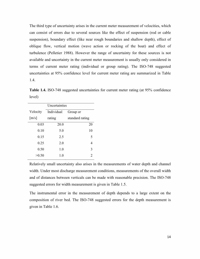
The third type of uncertainty arises in the current meter measurement of velocities, which

can consist of errors due to several sources like the effect of suspension (rod or cable

suspension), boundary effect (like near rough boundaries and shallow depth), effect of

oblique flow, vertical motion (wave action or rocking of the boat) and effect of

turbulence (Pelletier 1988). However the range of uncertainty for these sources is not

available and uncertainty in the current meter measurement is usually only considered in

terms of current meter rating (individual or group rating). The ISO-748 suggested

uncertainties at 95% confidence level for current meter rating are summarized in Table

1.4.

Table 1.4. ISO-748 suggested uncertainties for current meter rating (at 95% confidence

level)

Uncertainties

Velocity

[m/s]

Individual

rating

Group or

standard rating

0.03

0.10

0.15

0.25

0.50

>0.50

20.0

5.0

2.5

2.0

1.0

1.0

20

10

5

4

3

2

Relatively small uncertainty also arises in the measurements of water depth and channel

width. Under most discharge measurement conditions, measurements of the overall width

and of distances between verticals can be made with reasonable precision. The ISO-748

suggested errors for width measurement is given in Table 1.5.

The instrumental error in the measurement of depth depends to a large extent on the

composition of river bed. The ISO-748 suggested errors for the depth measurement is

given in Table 1.6.

15

Table 1.5. ISO-748 suggested uncertainties for width measurements (at 95% confidence

level)

Range of width

[m]

Absolute errors

[m]

Relative Error

[%]

0 to 100

150

250

0.3

0.5

1.2

±0.3

±0.4

±0.5

Table 1.6. ISO-748 suggested uncertainties for depth measurements (at 95% confidence

level)

Range of

depth [m]

Absolute

errors [m]

Relative error

[%]

Remarks

0.4 - 6

6 - 14

0.04

0.05

±0.7

±0.4

sounding rod

log-line and air- and wet line corrections

1.3.2 Uncertainty in discharge measurement by ADCP

In most cases, ADCP discharge measurement system is dramatically faster than

conventional discharge measurement systems and has comparable or better accuracy

(Simpson 2001). However, the ADCP discharge measurement is also affected by a

number of uncertainties, which can affect accuracy of total discharge measured by the

instrument. A major source of uncertainty arises due to the unmeasurable areas at the left,

right, top and bottom portions of the discharge measurement section as shown in Figure

1.2. González-Castro and Muste (2007) outlined other sources of errors in the ADCP,

which include: spatial averaging of the measurement, Doppler noise, velocity ambiguity

error, timing errors, side-lobe interference error, sound speed error, beam angle error,

boat speed error, sample timing error, near transducer error, reference boat velocity error,

depth error, cell mapping error, rotation error, edge estimation error, vertical velocity

distribution error, discharge model error, finite summation error, measuring environment

and operational errors. A framework for the quantification of uncertainty ranges in ADCP

16

is still under development (WMO 2008) and suggested uncertainty values for these

uncertainties are not available.

1.3.3 Uncertainty in stage measurement

The uncertainty in stage measurement depends upon the characteristics of gauging station

and water surface elevation. Since the stage can be measured directly, it is reasonable to

assume that errors in the measurement of stage are small compared to errors in the

discharge (Clarke 1999). However, displacement of measured values from the reference

point, caused by processes such as turbulent fluctuations, wind and stationary waves can

lead to error in the measured stage (Schmidt 2002). Uncertainty values in different

measurement instruments as suggested by Herschy (1995) are given in Table 1.7.

Table 1.7. Uncertainties for stage measurements at 95% confidence level (Herschy 1995)

Method Uncertainty

[mm]

By float operated punch tape recorder

By float operated autographic recorder

By point gauge, electrical tape gauge, tape

gauge etc

By reference vertical or inclined gauged

3

10

1

3

A source of uncertainty often neglected in stage measurement is the determination of

mean reference gauge height corresponding to the measured discharge. According to

Rantz et al. (1982), if the change in stage is uniform or no greater than 0.05 m, the mean

stage can be obtained by averaging the stage at the beginning and end of the

measurement. In the case of non-uniform stage, mean stage can be obtained by weighting

each stage by partial discharge. There is no suggested uncertainty range available for the

determination of mean stage.

17

1.4 Sources of uncertainty in stage-discharge relationship

1.4.1 Propagation of measurement uncertainty

As outlined in section 1.3, each of the discharge and stage measurements consists of

random and systematic uncertainties. The discharge values in particular consist of a

number of uncertainties arising out of measurement uncertainties of velocity, width and

depth. Therefore, the discharge values consist of aggregate of these individual

uncertainties. As the rating curves are established with the measurements of discharge

and stage, the measurement uncertainties propagate into the rating curve.

1.4.2 Change in river cross section

Another source of natural uncertainty in the stage-discharge relationship is due to change

in river cross-section. Rivers are affected by dynamic physical processes of erosion and

sedimentation. Discharge and stage measurements are made over a period of time,

usually over a few years. If the change in the cross section is not taken into account, it

introduces systematic error or bias in the regression data and affects the rating curve

established using the regression analysis.

1.4.3 Uncertainty due to hysteresis

A major source of uncertainty in the rating curve arises due to assumption of a single-

valued rating curve. In situations where a gauging station is located in sufficiently steep

gradient, rate of change of discharge is low and downstream channel has sufficient

capacity, the relationship between stage and discharge is sufficiently consistent with a

single-valued assumption (ISO 1100-2, 1998; Rantz et al. 1982). However, assumption of

the single-valued curve is not suitable if river flow is significantly affected by

unsteadiness in flood wave propagation. The phenomenon may lead to a looped form of

stage–discharge relationship which is commonly referred to as hysteresis. A number of

factors contribute to the form of looped rating curve which include acceleration of flow in

time and space, longitudinal bed slope, channel roughness and downstream boundary

condition (Henderson 1966; Cunge et al. 1980; Rantz et al. 1982; Chow et al. 1988;

Ponce 1989). Due to these reasons, river discharge is not just a function of stage and the

assumption of single valued stage-discharge relationship becomes inconsistent.

18

A typical looped rating curve as shown in Figure 1.3 is characterized by peak flow

always preceding peak stage and higher discharge in rising limb in comparison to falling

limb of a hydrograph. The effect is due to the slope of flood wave front, which is

significantly steeper on the rising limb compared to the falling limb, thus the flow is

accelerating on the rise and decelerating on the fall (ISO 1100-2, 1998, USACE, 1993).

The steeper slope in the rising limb allows a river channel to transit higher discharge at a

particular stage compared to the falling limb. The bed slope is another important factor

that affects the unsteady flow in rivers. The rating curves show more pronounced loops in

rivers with flat bed slope, and greater the slope, smaller is the deviation from the single

valued rating curve (Cunge et al. 1980). The channel roughness also affects shape of the

loop such that higher channel roughness leads to lower peak and wider loops compared to

lower channel roughness (Cunge et al. 1980).

Figure 1.3. Schematic representation of steady and unsteady state rating curves

After Chow et al. (1988)

1.5 Structure of this report

Chapter 2 of this report discusses the fuzzy set theory based methodology for the

uncertainty analysis. The rationale of the use of fuzzy sets for the uncertainty analysis is

described. Basic concepts of fuzzy sets including fuzzy numbers, membership functions,

fuzzy alpha cut, fuzzy arithmetic and fuzzy regression are introduced.

Dynamic or looped rating curve

Steady state rating curve

Q

h

Peak Discharge

Peak Stage

19

Chapter 3 of this report describes a fuzzy set theory based methodology for consideration

of different sources of uncertainty in the stage and discharge measurements and their

aggregation into a combined uncertainty. The uncertainty in individual measurements of

stage and discharge is represented using triangular fuzzy numbers and their spread is

determined according to the ISO-748 guidelines. The extension principle based fuzzy

arithmetic is used for the aggregation of various uncertainties into overall stage-discharge

measurement uncertainty. In addition, a fuzzified form of ISO-748 formulation is used

for the calculation of combined uncertainty and comparison with the fuzzy aggregation

method. This chapter also presents a methodology for the analysis of uncertainties in an

Acoustic Doppler current profiler discharge measurement. The methodology is based on

the representation of random uncertainties in discharge measurement at different sections

in terms of fuzzy numbers and aggregation into combined fuzzy uncertainty.

Chapter 4 of this report builds on the results of chapter 3, for the analysis of uncertainty

in stage-discharge relationship using fuzzy nonlinear regression. The methodology for

fuzzy nonlinear regression which is based upon fuzzy extension principle is described in

detail. All input and output variables as well as coefficients of the stage-discharge

relationship are considered as fuzzy numbers. Two different criteria are used for the

evaluation of output fuzziness: (i) the minimum spread; and (ii) the least absolute

deviation criteria.

Chapter 5 of this report analyzes the uncertainties in a looped rating curve with a

fuzzified form of Jones formula. A fuzzy set theory based methodology is investigated by

considering the parameters of Jones formula as fuzzy numbers. The spreads of

parameters of Jones formula is analyzed with a multi-objective optimization algorithm.

Chapter 6 of this report summarizes the major finding of this study and discusses

dominant sources of uncertainties in the measurement and rating curve. This chapter also

discusses means for the reduction of uncertainties.

20

CHAPTER 2

Uncertainty analysis using fuzzy set theory

2.1 Rationale for application of fuzzy sets

For the quantification of stage-discharge measurement uncertainties, the International

Organization for Standardization (ISO-748) suggests the range of values at 95%

confidence level for different sources of uncertainty. This recommendation is based on

investigations carried out since 1968. The ISO-748 recommends independent

determination of uncertainty in each measurement for the application to a particular case

study. However, in most cases, independent value of confidence interval in the

measurement is not available, which limits the applicability of statistical quantification of

the uncertainties. It is to be noted too that randomness is not the only source of

uncertainty in discharge measurements as they can be also affected by systematic

uncertainty, human error and other subjective uncertainties that cannot be treated in a

statistical framework. For example, the evaluation of individual current meter discharge

measurement on the basis of hydrographer observation can be subjective as each

measurement can receive different ratings based on the hydrographer’s perception

(Clemmens and Wahlin 2006). The ISO (1993) guide for expression of uncertainties has

recognized these limitations by distinguishing two different categories of uncertainties

according to method used to estimate their numerical values: Type A, method of

evaluation of uncertainty by the statistical analysis of series of observations, and Type B,

evaluation of uncertainty by means other than the statistical analysis of series of

observations.

The ISO-748 also provides a statistical framework for aggregation of confidence levels of

measurement uncertainties. The combined uncertainty is expressed as the ratio between

the sum of percentage errors in segment discharges and the sum of segment discharges

(Herschy 1995). However, such aggregation method only provides a means of combining

the confidence levels and cannot provide a confidence interval of the output unless the

21

probability distribution function that characterizes its dispersion is known (Ferrero and

Salicone 2003). Therefore, there are a number of limitations in the application of the

statistical methodology in the aggregation of the overall uncertainties in discharge and

stage measurements.

In addition to the measurement uncertainties, the stage-discharge relationship also

consists of natural uncertainties due to change in river cross sections, which can introduce

bias in the regression data. The hysteresis introduces non-uniqueness in the stage-

discharge relationship. The Jones formula (Jones 1916) is a popular method for

reproducing hysteresis in the stage-discharge relationship. However, the modeling of

hysteresis using Jones formula is affected by uncertainty due to simplifying assumptions

of the formula. These uncertainties due to bias, non-uniqueness and simplification in the

stage-discharge relationship cannot be directly expressed in the statistical framework

using confidence intervals. Therefore, probabilistic methods of uncertainty analysis are

not considered in this study.

The fuzzy set theory-based approach is explored in this study as an alternative way of

analyzing various uncertainties associated with measurements and the rating curve. The

fuzzy approach provides a non-probabilistic framework for representation of

uncertainties using vaguely defined boundaries of fuzzy sets. El-Baroudy & Simonovic

(2006) and Guyonnet et al. (2003) used fuzzy sets to treat uncertainties due to lack of

knowledge and scarcity of data, respectively. In recent years, the fuzzy sets have been

used for the expression of uncertainty in measurement by a number of researchers

(Mauris et al. 2001; Xia et al. 2000). The study by Xia et al. (2000) considered

application of fuzzy set for the estimation of uncertainty when the number of

measurements is very small and the probability distribution unknown. Mauris et al.

(2001) used fuzzy sets for the representation of vertical interpretation of probability

distribution and nested stacks of intervals as horizontal interpretation of distribution

function for representation of measurement uncertainty. The study also showed that fuzzy

representation of measurement uncertainty in terms of possibility distribution is

compatible with the ISO (1993) guide for expression of uncertainties, as it can

characterize dispersion of observed data and provide a confidence interval that contains

22

an important proportion of the observed values. Another approach for the consideration

of measurement uncertainties uses random-fuzzy variables (Ferrero and Salicone 2003;

2004; Urbanski and Wasowski 2003) to define random properties of uncertainties in

terms of probability distribution and systematic components in terms of possibility

function. However, in the absence of information on the random uncertainties, purely

fuzzy treatment can still be used.

The fuzzy set approach, known as fuzzy regression, can be used for addressing the non-

uniqueness in the relationship between dependent and independent variables. Due to the

non-unique characteristics of the stage-discharge relationship, it is more appropriate to

define the upper and lower uncertainty bands around the measurement values. It is also

appropriate to analyze a band of possible lower and upper values around the looped rating

curve developed by Jones formula. The fuzzy regression analysis can handle such a

problem by defining a band around the relationship in terms of possible upper and lower

values. Following the initial work by Tanaka et al. (1982), there are numerous

applications of fuzzy regression analysis in the recent years (e.g. Bárdossy et al. 1990;

Lee et al. 2001; D'Urso 2003; Kao and Chyu 2003; Mousavi et al. 2007).

The study therefore considers a fuzzy set theory based methodology for the consideration

of the uncertainties from the source and propagation of uncertainties in the rating curves.

The rest of this chapter describes the basic principles of fuzzy sets for handling

measurement and rating curve uncertainties.

2.2 Introduction to fuzzy set theory

Zadeh (1965) introduced the fuzzy set as a class of object with a continuum of grades of

membership. In contrast to classical crisp sets where a set is defined by either

membership or non-membership, the fuzzy approach relates to a grades of membership

between [0, 1], defined in terms of the membership function of a fuzzy number. Hence,

the classical notion of binary membership has been modified for the representation of

uncertainty in data.

The numerical values of fuzzy numbers in a domain are assigned by membership level,

which may take any value between 0 and 1, with no membership at 0 and full

23

membership at 1. In mathematical terms, assuming X as a universe set of x values

(elements), then A as a fuzzy subset of X, in ordered pairs is given by:

( ) [ ]{ }1,0)(,;)(, ∈∈= xXxxxA AA µµ (2.1)

where, )(xAµ is the grade of membership of x in the fuzzy subset A.

A membership function can be of any shape depending on the type of a fuzzy set it

belongs to. The only condition a membership function must satisfy is it should vary

between 0 and 1.

2.2.1. Fuzzy Numbers

Fuzzy numbers are normal and convex fuzzy sets, whose numerical values in the domain

are assigned by specific grades of membership. While Boolean operations such as union

and intersection can be carried out on any fuzzy sets, the fuzzy numbers can be used to

perform arithmetic operations such as addition, subtraction, multiplication and division.

The commonly used fuzzy numbers are outlined below.

i. Triangular fuzzy number. It is based on fuzzy number A = (a, b, c) with a ≤ b ≤ c.

The interval (a, c) is the support of the triangular fuzzy number. This membership

function is shown in Figure 2.1 and given by:

≥

≤≤−−

≤≤−−

≤

=

cx

cxbbc

xc

bxaab

ax

ax

xA

if0

if

if

if0

)(µ (2.2)

ii. Trapezoidal fuzzy number. The function is based on fuzzy number A = (a, b, c, d),

where a ≤ b ≤ c ≤ d. The interval (a, d) is the support of the trapezoidal fuzzy number.

This membership function is shown in Figure 2.2 and given by:

≥

≤≤−−

≤≤

≤≤−−

≤

=

dx

dxccd

xd

cxb

bxaab

ax

ax

xA

if0

if

if1

if

if0

)(µ (2.3)

24

Figure 2.1. Triangular fuzzy number Figure 2.2. Trapezoidal fuzzy number

iii. Left-Right (L-R) fuzzy number. The linear function used in the definition of the

triangular fuzzy numbers may be replaced by a monotonic function. This is called Left-

Right or L-R representation of fuzzy numbers (Dubois and Prade 1980). For example,

coefficient A is expressed as ( ) m fA βα ,,ˆ = , where m is the central value and α and β

are the left and right spreads respectively. The membership function )(xAµ , of the

triangular L-R fuzzy number is given by equation 2.4 and shown in Figure 2.3 (D'Urso

2003):

>+≤≤−

−

>≤≤−−

−=

0,for1

0,for1

)(

βββ

αααµ

mxmmx

mxmxm

xA

(2.4)

α

1

0 x

µA(A)

βm Figure 2.3. Triangular membership function of L-R fuzzy number

2.2.2 Alpha level cut

Fuzzy alpha-level cut (α – cut) can be used for resolving fuzzy numbers into crisp

numbers, so that crisp mathematical operations such as addition, subtraction, division,

0.0

0.2

0.4

0.6

0.8

1.0

1.2

a b c d0.0

0.2

0.4

0.6

0.8

1.0

1.2

a b c

25

square and square root can be performed (Simonovic 2008). An example of fuzzy number

with α – cut and its support is shown in Figure 2.4. Let an α – cut intersect the

membership function of a fuzzy number at two points a1 and a2 (a1, a2ෛ A). Then, the

subset Aα contains all possible values of the fuzzy variable A, including and between a1

and a2, which are referred to as the lower and upper bounds of the α – cut. The subset Aα

also contains a set of elements, which have at least a membership value greater than or

equal to α, as given by:

{ }αµα ≥∈= )(, AAaA A (2.5)

Aαα

1

α - level cut

0 xa1 a2

µA(A)

Figure 2.4. Fuzzy number and α level cut

2.2.3 Fuzzy arithmetic

The fuzzy alpha level cut based fuzzy arithmetic provides a mean to generalize crisp

mathematical operations to fuzzy sets. For the fuzzy arithmetic operations, two fuzzy

numbers A and B, are considered at α – level: Aα = [a1, a2], Bα = [b1, b2].

The individual arithmetic operations on the α – cut of A and B can be defined in terms of

following equations (Klir 1997; Simonovic 2008):

] ,[ ] ,[ ] ,[ 22112121 bababbaa ++=+ (2.6)

] ,[ ] ,[ ] ,[ 12212121 bababbaa −−=− (2.7)

)],, ,max(),,, ,[min( ] ,[ *] ,[ 22122111221221112121 bababababababababbaa = (2.8)

26

],[0for ,,,,max, ,,,min ] ,[/ ] ,[ 21

2

2

1

2

2

1

1

1

2

2

1

2

2

1

1

12121 bb

b

a

b

a

b

a

b

a

b

a

b

a

b

a

b

abbaa ∉

= (2.9)

For the calculation of the fuzzy square root, Salicone (2007) proposed the following

relation:

[ ][ ][ ]

≤≤

><

≤≤

=

0 when -- --

0,0 when --

0n whe

] ,[

2121

2121

2121

21

aaa,a

aaa,a

aaa ,a

aa (2.10)

Similarly, for the calculation of fuzzy square, the following equation can be used:

[ ][ ][ ]

0 when -

0,0 when -

0n whe

] ,[

21

2

2

2

1

21

2

1

2

2

21

2

2

2

1

2

21

≤≤−

><

≤≤

=

aaa,a

aaa,a

aaa,a

aa (2.11)

2.2.4 Fuzzy regression

The classical regression approach defines the relationship between the independent and

dependent variables in terms a mathematical relationship, which can be expressed as:

ipPii xAxAAy +++= ...110 (2.12)

Where y is the dependent variable, x is the independent variable, A is the coefficient of

regression, p is the number of independent variables and ni ...,2,1= is the observation

of each independent variable.

In real world problems, the relationships between the independent and dependent

variables can rarely be expressed in terms of simple linearized equation such as (2.12).

The relationships are often affected by data uncertainties and complex physical processes,

which cannot be represented by simplified linear or nonlinear equations. It is more

appropriate to define such relationships in terms of credible bands of lower and upper

scenarios to represent the uncertainties in the data and complexities in the relationship.

27

Fuzzy extension principle (Zadeh, 1965) based fuzzy regression approach can handle

such a problem by defining the coefficients of the relationships as fuzzy numbers, which

can be expressed as:

ipPii xAxAAy ˆ...ˆˆ110 +++= (2.13)

The L-R (left–right) representation of fuzzy number provides a suitable means for

representing the fuzzy coefficient jA . Due to measurement uncertainties of the

independent and dependent variables, it may be necessary to define the variables and well

as coefficients of the variables and fuzzy numbers, which can be expressed as:

ipPii xAxAAy ~ˆ...~ˆˆ~110 +++= (2.14)

The left and right spreads of the L-R fuzzy number can be extended to incorporate the

uncertainty not captured in available data sets using a degree of belief, H (Chang and

Ayyub 2001). According to this approach, each of the observed data points must be

within the band around estimated regression curves at H level as shown in Figure 2.5.

The spread of the membership function and, hence, the fuzziness of the regression

variables can be controlled by specifying the H level between 0 and 1. Accordingly, for

the degree of belief H, the left and right spreads of the L-R fuzzy number A and B can be

expressed as:

)1(ˆ)1( HmAHm jjjjj −+≤≤−− βα (2.15)

The spread of the fuzzy regression curve also depends upon the reference point of the

corresponding independent variable to which fuzzy regression analysis is performed. For

example, if two fuzzy regression analyses are performed with the reference points at; (i)

the minimum value of the independent variable and (ii) the maximum value of the

independent variable; the spread of the regression curve will be higher around the

maximum of the independent variable in case (i) compared to the case (ii). Depending

upon the regression data, one or more reference points may be used, where the regression

is believed to be the most accurate. The reference point should be selected where the

regression is supposed to be the crispest, like around the average or the maximum value

(Bárdossy et al. 1990).

28

Figure 2.5. Representation of degree of belief H in L-R fuzzy number

H

)1( Hm jj −−α

1

0 A jm

)1( Hm jj −+ β

jjm β+ jjm α−

µ A ( A )

Available

data range

29

CHAPTER 3

Analysis of uncertainties in stage-discharge measurements

The chapter presents two case studies on the analysis of stage-discharge measurement

uncertainties. The first case study presents a combined methodology for uncertainty

analysis of discharge and stage measurement. The methodology uses data from current

meter discharge measurement and float operated stage measurement from Thompson

River near Spences bridge in British Columbia, Canada. The second case study presents a

methodology for uncertainty quantification in discharge measurement using Acoustic

Doppler current profiler from Richelieu River in Quebec, Canada.

3.1 Methodology for uncertainty analysis

3.1.1 Analysis of current meter discharge measurement uncertainty

3.1.1.1 Aggregation of uncertainties using fuzzy arithmetic

For consideration of uncertainties in measurement of depth, width and current meter

measurement of velocity, each of measurement quantities is expressed as a symmetrical

triangular fuzzy number with the spread given by percentage fraction between –xi and xi,

and central value at 0 as shown in Figure 3.1.

As described in chapter 1, uncertainty in the measurement of velocity consist of three

different sources: (i) uncertainty in the number of points on a vertical pX ; (ii) current

meter rating cX ; and (iii) time of exposure eX . Each of these uncertainties is

independent of each other, therefore, the total uncertainty can be considered to be less

than arithmetic sum of individual uncertainties. Therefore, a method based on the ISO-

748 is used, which calculates the total uncertainty as the square root of sum of squares of

individual uncertainties. As the individual uncertainties are expressed in terms of

percentage fraction between –xi and xi, and central value at 0, the combined fuzzy

30

uncertainty in the mean velocity iv is calculated as the sum of total uncertainties plus

unity, multiplied by the crisp mean value of velocity measurement iv :

( ) ( ) ( )

+++=

222 ˆˆˆ1ˆecpii XXXvv (3.1)

1

0x

- xi

µA(A)

xi

Figure 3.1. Expression of measurement uncertainty in terms of fuzzy number

Similarly, fuzzy number of the width measurement ib

and depth measurement

id considering the measurement uncertainties is expressed as:

( )bii Xbb ˆ1ˆ += (3.2)

( )dii Xdd ˆ1ˆ += (3.3)

Here bX and dX are the fuzzy numbers of uncertainties in width ib and depth id

measurements, respectively.

The computation of discharge using mid section velocity area method is the standard in

Canada (Pelletier 1988). For the width measurement from a common reference point, the

discharge Q measurement using mid section method may be expressed as:

∑−

=

−+

−=

1

2

11

2

n

i

i

ii

i dbb

vQ (3.4)

31

Using the fuzzified values of velocity, depth and discharge, from equations (3.1), (3.2)

and (3.3), the total discharge is calculated as a fuzzy number Q :

∑−

=

−+

−=

1

2

11 ˆ2

ˆˆˆˆ

n

i

i

ii

i dbb

vQ (3.5)

In order to take into consideration the uncertainty due to limited number of verticals, mX ,

expressed as a fraction, the total uncertainty in the discharge measurement is calculated

using the following relationship:

( )mtot XQQ ˆ1ˆˆ += (3.6)

3.1.1.2 Aggregation of uncertainties using fuzzified ISO method

For the comparison with the above method, aggregation of uncertainties using fuzzy

variables with a conventional treatment of measurement, uncertainties according to ISO-

748 is used. In this case, instead of aggregation of confidence level of uncertainty, each

of the uncertainties is fuzzified and aggregated using fuzzy arithmetic. According to the

ISO-748 suggested formulation, a combination of confidence level of uncertainties is

expressed as:

( )( ) ( ) ( ) ( ) ( ) ( ){ }[ ]

( )

21

2

1

1

2122222

2

++++

+±=

∑

∑

=

=m

i

iii

m

i

ecpdbiii

mQ

vdb

XXXXXvdb

XX (3.7)

It is to be noted that the equation (3.7) is different from equation given in ISO-748. The

derivation of the equations for the aggregation of uncertainties according to the ISO-748

is documented in Herschy (1995), where two different forms of equations are listed. The

equation without squaring of the terms on the right hand side is used in this study as it

confirms with definition of total uncertainty as a ratio of sum of percentage errors in the

segment discharges to the sum of the segment discharges. Hence, the original form of

equation by Herschy (1995) is used for the aggregation of uncertainties. Expressing each

uncertainty in terms of fuzzy numbers leads to:

32

( )( ) ( ) ( ) ( ) ( ) ( ){ }

( )

21

2

1

1

2122222

2

ˆˆˆˆˆ

ˆˆ

++++

+±=

∑

∑

=

=m

i

iii

m

i

ecpdbiii

mQ

vdb

XXXXXvdb

XX (3.8)

The total uncertainty in discharge measurement is expressed as:

( )Qtot XQQ ˆ1ˆ += (3.9)

3.1.2 Analysis of Acoustic Doppler current profiler discharge measurement

uncertainties

As described in chapter 1, the measurement of discharge using Acoustic Doppler current

profiler (ADCP) consists of number of different sources of uncertainties. A major source

of uncertainty arises due to unmeasurable areas at the left, right, top and bottom portions

of the discharge measurement section as shown in Figure 1.2. However, suggested

uncertainty values for these uncertainties are not available.

The random sources of uncertainties in the ADCP discharge measurement can be

quantified from the ADCP measurements, which are usually undertaken in a number of

tracks. Based on the quantified uncertainties, measurements in each section in a channel

can be expressed as a fuzzy number:

( )iii XQQ ˆ1ˆ += (3.10)

where iQ is the discharge measurement at any section of river channel, and iX and iQ

are the fuzzy numbers of uncertainties and discharge, respectively at the measurement

section.

From the uncertainty in each portion of discharge measurement defined by equation

(3.10), the total uncertainty in discharge measurement by ADCP can be expressed as:

rightbottommiddletoplefttotal QQQQQQ ˆˆˆˆˆˆ ++++= (3.11)

where, leftQ , topQ , middleQ , bottomQ and rightQ are fuzzy numbers of discharge measurement

at left, top, middle, bottom and right sections. totalQ is the fuzzy number of total discharge.

33

3.1.3 Analysis of stage measurement uncertainties

In the case of stage measurement, two different sources of uncertainty are considered: (i)

error in the measuring instrument, insX ; and (ii) error in the determination of mean

reference gauge height corresponding to the measured discharge, refX . Since the

uncertainty (ii) is dependent on (i), the combined uncertainty can be calculated as the sum

of uncertainties (i) and (ii). Therefore the aggregated uncertainty in stage measurement


( ){ }refins XXhh ˆˆ1ˆ ++= (3.12)

where, h is the measured stage and h is the fuzzified stage.

3.2 Case study 1: Combined uncertainty analysis of current meter discharge and

stage measurements

Stage and discharge measurements from Thompson River near Spences bridge from 1970

to 2000 are used for a combined fuzzy analyses of measurement uncertainties. Thompson

River is a major tributary of the Fraser River in British Columbia, Canada with a gross

drainage area of 54,900 km2

at the gauging station. The station is located in a narrow

gorge with well defined banks. The analysis of the river cross sections from 1970 to

2000, showed a very little change in channel geometry indicating the cross section to be

very stable.

The case study uses 58 measurements of stage and discharge values for the rating curve

uncertainty analysis. The minimum, mean and maximum values of stage data are 0.44 m,

3.75 m and 8.93 m, respectively. The minimum, mean and maximum discharge values

used in the analysis are 155 m3/s, 1392 m

3/s and 4081 m

3/s, respectively. Individually

rated current meter is used for the discharge measurements with 20-30 observation

verticals in a cross section. Only a single point on each vertical is used for the estimation

of mean velocity. The total discharge is calculated using mid-section method.

The available information from the Spences bridge gauge and general practice of

discharge measurement in Canada (Terzi 1981, Pelletier 1988) are used in the analyses.

The ISO-748 suggested random uncertainty values (at 95% confidence level) are used as

34

a reference for the expression of each of the uncertainty in terms of triangular fuzzy

number. As already outlined, ISO-748 recommends determination of the values

independently for the application to a particular case. Therefore, in order to account for

the lack of information on random uncertainties and possible systematic uncertainties, the

spread of each fuzzy number, in this case, is increased by 50%. Therefore, the fuzzy

number of each of the uncertainty sources is viewed as a combination of both; the

random and systematic uncertainty. The left or right spread (one half of the support) of

the symmetrical triangular fuzzy number taken for each of the errors is given in Table

3.1.

Table 3.1. Half of the support of fuzzy number of errors in discharge measurement due to

different uncertainty sources

Uncertainty source Half of support of fuzzy

number (%)

Limited number of verticals (20-30)

Limited number of points in a vertical (single point)

Limited exposure time (one minute)

Current meter rating (individual rating for velocity > 0.5

m/s)

Depth measurement (0.4-6 m)

Width measurement (0-100 m)

7.5-4.5

22.5

9.0

1.5

1.05

0.45

In the case of uncertainty in the stage measurement, half of the support of fuzzy number

of errors considered is summarised in Table 3.2.

35

Table 3.2. Half of the support of the fuzzy number of errors in stage measurement due to

different uncertainty sources

Uncertainty source Half of the support of fuzzy number

(mm)

Measurement instrument

Determination of mean reference gauge height

15

15

3.2.1 Results and discussion

3.2.1.1 Fuzzy arithmetic aggregation method

The aggregation of uncertainties using fuzzy variables leads to nonlinear fuzzy numbers

of discharge values. The membership functions of the largest measured discharge and

corresponding stage are shown in Figures 3.2 and 3.3, respectively. The results show high

uncertainty in discharge due to measurement uncertainties characterized by wide support

of discharge fuzzy number. The central value of discharge and stage fuzzy numbers

represents the values without consideration of uncertainty. The left and right spreads

represent the total uncertainties in the measurement. The fuzzy numbers can be

interpreted in terms of membership levels, with 0 as the highest uncertainty, i.e., the

extreme possible measurement value. The closer the membership level is to 1, the lower

is the uncertainty.

The independent (non-interactive) measurements of discharge and stage are combined to

form a joint fuzzy number of the corresponding measurements. This leads to a tri-

dimensional representation of the fuzzy number as shown in Figure 3.4. The joint

membership function of the stage and discharge values provides a visualization of

uncertainties in stage and discharge at any membership level. The joint membership

function of the fuzzy numbers Qhµ is given by:

)min( , hQQh µµµ = (3.13)

where, Qµ is the discharge membership level and hµ is the stage membership level.

36

Figure 3.5 shows a ‘top view’ of the uncertainty in observed stage and discharge values

represented by spread of joint membership functions of fuzzy numbers. Each rectangle in

Figure 3.5 represents four points a, b, c and d with membership level 0 as shown in

Figure 3.4. It is evident from Figure 3.5 that the spread of discharge fuzzy numbers

increases with the higher discharge while the spread of the stage fuzzy numbers remains

constant. This is due to the fact that uncertainties in each of the elements of discharge

measurement (velocity, depth and width) are expressed in terms of percentage values,

while constant uncertainty is used for all stage values.

2500 3000 3500 4000 4500 5000 5500 60000

0.1

0.2

0.3

0.4

0.5

0.6

0.7

0.8

0.9

1

Discharge (m3/s)

Mem

bers

hip

level


using fuzzy arithmetic aggregation method

37

8.88 8.9 8.92 8.94 8.96 8.980

0.1

0.2

0.3

0.4

0.5

0.6

0.7

0.8

0.9

1

Stage (m)

Mem

bers

hip

level

Figure 3.3. Membership function of fuzzy number of maximum observed stage using

fuzzy arithmetic aggregation method

25003000

35004000

45005000

55008.9

8.92

8.94

8.96

8.98

0

0.2

0.4

0.6

0.8

1

Discharge (m3/s)Stage (m)

Mem

bers

hip

level

a

b

c

d

Figure 3.4. Joint membership function of maximum observed stage and discharge in

terms of tri-dimensional representation of fuzzy number (fuzzy arithmetic aggregation

method)

38

0 1 2 3 4 5 6 7 8 90

1000

2000

3000

4000

5000

6000

Stage (m)

Dis

charg

e (m

3/s

)

Figure 3.5. Uncertainty in observed stage and discharge represented by spread of joint

membership functions using fuzzy arithmetic aggregation method

3.2.1.2 Fuzzified ISO method

The result of fuzzified ISO method also shows the large spread of the fuzzy number of

largest measured discharge as shown in Figure 3.6. In this case also, there is increase in

spread of discharge fuzzy numbers with the higher discharges as shown in Figure 3.7. A

comparison of the left and right spread of fuzzy numbers for the minimum, mean and

maximum discharge is given in Table 3.3. It can be seen from the Table that the spreads

are higher in the case of fuzzy aggregation method in comparison to the ISO method.

This is due to the fact that aggregation of uncertainty using fuzzy arithmetic method uses

direct combination of fuzzy numbers of different uncertain quantities and there is no

reduction of uncertainty. In the case of the ISO method, the fuzzified form of the ISO

equation (Equation 3.10) is used, which combines the fuzzy numbers of uncertainties as a

square root of the sum of squares of all the uncertainties. Therefore, there is reduction of

uncertainties in the ISO method. It is to be noted too that the ISO method leads to a linear

fuzzy number of discharge, and the fuzzy aggregation leads to a nonlinear fuzzy number.

The right spread of the fuzzy numbers for minimum, mean and maximum are higher than

the left spread in the case of fuzzy aggregation method, while the left and right spreads

are equal in the case of fuzzified ISO method.

39

2500 3000 3500 4000 4500 5000 5500 60000

0.1

0.2

0.3

0.4

0.5

0.6

0.7

0.8

0.9

1

Discharge (m3/s)

Mem

bers

hip

Level


using fuzzified ISO method

0 1 2 3 4 5 6 7 8 90

1000

2000

3000

4000

5000

6000

Stage (m)

Dis

charg

e (m

3/s

)

Figure 3.7. Uncertainty in the observed stage and discharge represented by spread of

joint membership functions using fuzzified ISO method

40

Table 3.3. Comparison of the left and right spreads of the fuzzy numbers of discharge

using fuzzy aggregation and fuzzified ISO method

Left spread (m3/s) Right Spread (m

3/s)

Min Mean Max Min Mean Max

Fuzzy arithmetic aggregation method 45 406 1211 49 459 1361

Fuzzified ISO method 38 338 1013 38 338 1031

3.2.1.3 Recommendations for reduction of uncertainties in the case study

The possibilities of reducing total uncertainty in discharge measurement is analyzed by

considering different spreads of membership functions of the uncertainty sources. Three

parameters with highest range of uncertainty values are chosen for the analyses, which

include: approximation due to the limited number of verticals, velocity uncertainties due

to the limited numbers of points on a vertical and the measurement exposure time.

Different values of uncertainties used for the analyses are summarized in Table 3.4.

Table 3.4. Values of uncertainties used for the uncertainty reduction analyses

Criteria Uncertainty values in %

No of verticals 6.0 4.5 3.0 1.5

No of points in a vertical 22.5 15.0 10.5 2.5

Exposure time 9.0 7.5 6.0 3.0

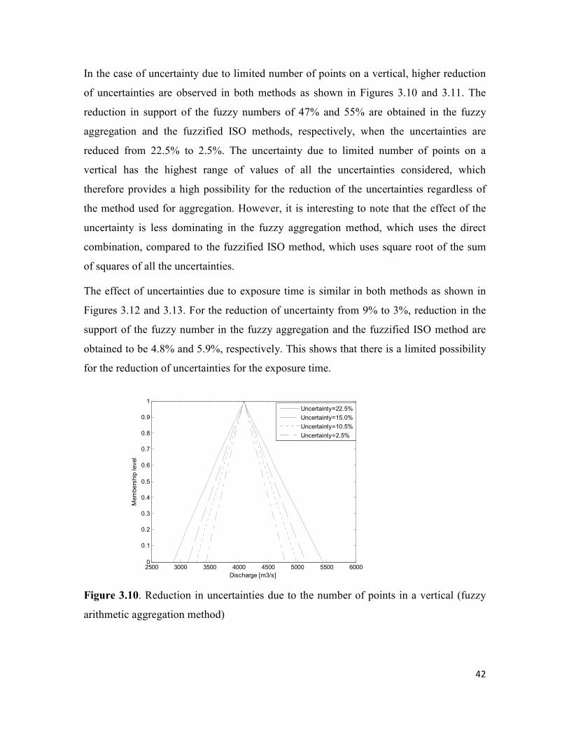
Figures 3.8 and 3.9 show the effects of uncertainty in the number of verticals for fuzzy

aggregation and fuzzified ISO methods, respectively. For the reduction of uncertainty

from 6% to 1.5%, the reduction in support of fuzzy number in the fuzzy aggregation and

the fuzzified ISO method are obtained to be 13.4% and 2.5%, respectively. This shows

that the uncertainty due to limited number of verticals has a more significant effect with

the application of fuzzy aggregation method than with the application of the fuzzified

ISO method. This difference is due to the fact that ISO method combines the

41

uncertainties as a square root of the sum of squares of all the uncertainties and the highest

value of uncertainty dominates. This leads to a lower effect of elements with the low

uncertainty level.

2500 3000 3500 4000 4500 5000 5500 60000

0.1

0.2

0.3

0.4

0.5

0.6

0.7

0.8

0.9

1

Discharge [m3/s]

Mem

bers

hip

level

Uncertainty=6.0%

Uncertainty=4.5%

Uncertainty=3.0%

Uncertainty=1.5%

Figure 3.8. Reduction in uncertainties in the number of verticals (fuzzy arithmetic

aggregation method)

2500 3000 3500 4000 4500 5000 5500 60000

0.1

0.2

0.3

0.4

0.5

0.6

0.7

0.8

0.9

1

Discharge [m3/s]

Mem

bers

hip

level

Uncertainty=6.0%

Uncertainty=4.5%

Uncertainty=3.0%

Uncertainty=1.5%

Figure 3.9. Reduction in uncertainties in the number of verticals (fuzzified ISO method)

42

In the case of uncertainty due to limited number of points on a vertical, higher reduction

of uncertainties are observed in both methods as shown in Figures 3.10 and 3.11. The

reduction in support of the fuzzy numbers of 47% and 55% are obtained in the fuzzy

aggregation and the fuzzified ISO methods, respectively, when the uncertainties are

reduced from 22.5% to 2.5%. The uncertainty due to limited number of points on a

vertical has the highest range of values of all the uncertainties considered, which

therefore provides a high possibility for the reduction of the uncertainties regardless of

the method used for aggregation. However, it is interesting to note that the effect of the

uncertainty is less dominating in the fuzzy aggregation method, which uses the direct

combination, compared to the fuzzified ISO method, which uses square root of the sum

of squares of all the uncertainties.

The effect of uncertainties due to exposure time is similar in both methods as shown in

Figures 3.12 and 3.13. For the reduction of uncertainty from 9% to 3%, reduction in the

support of the fuzzy number in the fuzzy aggregation and the fuzzified ISO method are

obtained to be 4.8% and 5.9%, respectively. This shows that there is a limited possibility

for the reduction of uncertainties for the exposure time.

2500 3000 3500 4000 4500 5000 5500 60000

0.1

0.2

0.3

0.4

0.5

0.6

0.7

0.8

0.9

1

Discharge [m3/s]

Mem

bers

hip

level

Uncertainty=22.5%

Uncertainty=15.0%

Uncertainty=10.5%

Uncertainty=2.5%

Figure 3.10. Reduction in uncertainties due to the number of points in a vertical (fuzzy

arithmetic aggregation method)

43

2500 3000 3500 4000 4500 5000 5500 60000

0.1

0.2

0.3

0.4

0.5

0.6

0.7

0.8

0.9

1

Discharge [m3/s]

Mem

bers

hip

level

Uncertainty=22.5%

Uncertainty=15.0%

Uncertainty=10.5%

Uncertainty=2.5%

Figure 3.11. Reduction in uncertainties due to the number of points in a vertical

(fuzzified ISO method)

2500 3000 3500 4000 4500 5000 5500 60000

0.1

0.2

0.3

0.4

0.5

0.6

0.7

0.8

0.9

1

Discharge [m3/s]

Mem

bers

hip

level

Uncertainty=9%

Uncertainty=7.5%

Uncertainty=6%

Uncertainty=3%

Figure 3.12. Reduction in uncertainty due to exposure time (fuzzy arithmetic aggregation

method)

44

2500 3000 3500 4000 4500 5000 5500 60000

0.1

0.2

0.3

0.4

0.5

0.6

0.7

0.8

0.9

1

Discharge [m3/s]

Mem

bers

hip

level

Uncertainty=9.0%

Uncertainty=7.5%

Uncertainty=6.0%

Uncertainty=3.0%

Figure 3.13. Reduction in uncertainty due to exposure time (fuzzified ISO method)

3.3 Case study 2: Uncertainty analysis of Acoustic Doppler current profiler

discharge measurements

The second case study presents a methodology for uncertainty quantification in discharge

measurement using Acoustic Doppler current profiler. We use seven ADCP measurement

data from Richelieu River in Quebec, Canada. Each of the measurements was repeated in

4-5 tracks, based on which ensemble of discharge at each section in the river channel

were calculated. We use the discharge measurement values from different tracks to

calculate the uncertainties at 95% confidence intervals. The calculated 95% confidence

interval uncertainty values are summarized in Table 3.5.

Table 3.5. ADCP measurements at 95% confidence interval

Measurement section Uncertainties [%]

Left

Top

Middle

Bottom

Right

43.20

1.95

0.58

1.22

37.80

45

Based on calculated uncertainty values, measurements at each section in a river channel

is defined as fuzzy numbers with both the left and right spreads of the fuzzy number of

uncertainties increased by 50%. An example of fuzzy numbers of discharge measurement

at different measurements sections are shown in Figure 3.14. Based on the defined

uncertainties at different sections in a river channel, the total uncertainty is calculated

using fuzzy arithmetic as shown in Figure 3.15.

It is to be noted that the uncertainties quantified in the given example only consists of

random uncertainties. However, the method can be adapted to quantify other sources of

random uncertainties as outlined in section 13.2 as well as systematic uncertainties. It can

also be seen that the ADCP discharge measurement uncertainty (Figure 3.15) is very

small compared to total uncertainty using current meter measurement (Figure 3.4).

Although the uncertainties in the ADCP does not incorporate different sources of possible

uncertainties, it can still be expected that the total uncertainty in the measurement will

still remain small compared to the current meter discharge measurement uncertainty.

46

Left Q

0

0.2

0.4

0.6

0.8

1

1.2

0.0 0.5 1.0 1.5

Discharge [m3/s]

Membership Level

Top Q

0

0.2

0.4

0.6

0.8

1

1.2

134.0 136.0 138.0 140.0 142.0 144.0 146.0

Discharge [m3/s]

Membership Level

Measured Q

0

0.2

0.4

0.6

0.8

1

1.2

770.0 775.0 780.0 785.0 790.0

Discharge [m3/s]

Membership Level

Bottom Q

0

0.2

0.4

0.6

0.8

1

1.2

97.0 98.0 99.0 100.0 101.0 102.0

Discharge [m3/s]

Membership Level

Right Q

0

0.2

0.4

0.6

0.8

1

1.2

0.0 1.0 2.0 3.0 4.0

Discharge [m3/s]

Membership Level

Figure 3.14. ADCP Discharge measurement uncertainties at different sections in a river

channel

47

Total Q

0

0.2

0.4

0.6

0.8

1

1.2

1000.0 1010.0 1020.0 1030.0 1040.0

Discharge [m3/s]

Membership Level

Figure 3.15. Total ADCP Discharge measurement uncertainty

48

CHAPTER 4

Fuzzy nonlinear regression analysis of stage-discharge relationship

This chapter presents a methodology for the analysis of uncertainty in a stage-discharge

relationship. The methodology builds on the results of chapter 3, where the measurement

uncertainties of stage and discharge are defined as fuzzy numbers, to define the lower and

upper bounds of the stage discharge relationship. The same discharge and stage data from

Thompson River near Spences bridge in British Columbia, Canada is used for the

analysis.

4.1 Methodology for fuzzy regression analysis of stage-discharge relationship

4.1.1 Derivation of fuzzy regression equations for stage-discharge relationship

The relationship between the stage, hi and the discharge, Qi is established by statistical

regression analysis using a number of simultaneous observations of stage and discharge

and is expressed in the mathematical form as:

B

ii AhQ = (4.1)

where A and B are the coefficients of the relationship.

Expressing the stage and discharge values, as well as regression coefficients, as fuzzy

numbers leads to:

B

ii hAQˆ~ˆ~

= (4.2)

The membership functions of fuzzy discharge and stage variables, iQ~

and ih~

, can be

derived from the measurement uncertainties. The membership functions of the fuzzy

coefficients A and B can be evaluated using fuzzy regression analysis, which is based on

fuzzy extension principle (Zadeh 1965). The L-R (left–right) representation of fuzzy

number as defined in chapter 2.1.1 provides a suitable means for representing the fuzzy

coefficients. As defined in section 2.2.4, it may be necessary to extend the spread of the

49

L-R fuzzy number to incorporate the uncertainty not captured in available data sets using

a degree of belief, H. Accordingly, for the degree of belief H, the left and right spreads of

the L-R fuzzy number A and B can be expressed as:

)1(ˆ)1( HmAHm AAAA −+≤≤−− βα (4.3)

)1(ˆ)1( HmBHm BBBB −+≤≤−− βα (4.4)

The spread of discharge fuzzy number iQ and stage fuzzy number ih obtained from

measurement uncertainty analysis (chapter 3) can be expressed as follows:

iiii QQiQQ mQm βα +≤≤−~

(4.5)

iiii hhihh mhm βα +≤≤−~

(4.6)

Considering the reference point for stage value as refh , as outlined in chapter 2.2.4, leads

to the following modification of equation 4.6:

i

i

i

i

h

ref

h

ref

ih

ref

h

h

m

h

h

h

mβα +≤≤−

~

(4.7)

For the derivation of the lower and upper bounds of the stage-discharge relationship, the

results of stage and discharge measurement uncertainty analysis as described in chapter 3

can be used. Based on the uncertainty plot of combined uncertainty of stage and

discharge measurement as shown in Figure 3.5, we derived conditions for fuzzy

regression. From Figure 3.5, it can be seen that the lower bound of fuzzy rating curve will

intersect with zero stage membership value at boundary of right spread and zero

discharge membership value at boundary of left spread. Similarly, the upper bound of

fuzzy rating curve will intersect with zero stage membership value at the boundary of left

spread and the zero discharge membership value at the boundary of right spread.

Therefore, we combined equations (4.3), (4.4), (4.5), (4.7) and (4.2), so that the lower

bound of fuzzy rating curve intersects with the zero stage membership value at the

boundary of right spread and the upper bound intersects with zero stage membership

value at the boundary of left spread. This leads to the expressions for the lower and upper

bounds of the fuzzy regression curve in the following form:

50

{ }{ }

ii

bb

i

i

QQ

Hm

h

ref

h

aa mh

mHm αβα

α

−≤

+−−

−− )1(

)1( (4.8)

{ }{ }

ii

bb

i

i

QQ

Hm

h

ref

h

aa mh

mHm βαβ

β

+≥

−−+

−+ )1(

)1( (4.9)

For most gauging stations it is necessary to consider two or more curves for a reasonable

fit of the measured stage and discharge data. Therefore, we consider two curves, for low

and high flows, meeting at a break point breakh in equation (4.2):

breaki

B

ii hhhAQ <= for~ˆ~

1ˆ

1 (4.10)

breaki

B

ii hhhAQ >= for~ˆ~

2ˆ

2 (4.11)

breaki

B

i

B

i hhhAhA == for~ˆ~ˆ 21

ˆ

2

ˆ

1 (4.12)

where the indices 1 and 2 denote the low and high range of the measurement data.

The consideration of two curves meeting at a point breakh leads to the expression of

equation (4.8) and (4.9) as follows:

{ }{ }

{ }{ } breaki

QQ

Hm

h

ref

h

aa

QQ

Hm

h

ref

h

aa

hh

mh

mHm

mh

mHm

ii

bb

i

i

ii

bb

i

i

<

+≥

−−+

−≤

+−−

−+

−−

for

)1(

)1(

)1(

11

)1(

11

11

11

βαβ

αβα

β

α

(4.13)

{ }{ }

{ }{ } breaki

QQ

Hm

h

ref

h

aa

QQ

Hm

h

ref

h

aa

hh

mh

mHm

mh

mHm

ii

bb

i

i

ii

bb

i

i

>

+≥

−−+

−≤

+−−

−+

−−

for

)1(

)1(

)1(

22

)1(

22

22

22

βαβ

αβα

β

α

(4.14)

In addition, the curves for low and high flow data should also meet at lower and upper

bounds as well as central value of the relationship curve. This leads to the following

additional condition:

51

{ }{ }

{ }{ }

{ }{ }

{ }{ }

breaki

m

ref

h

a

m

ref

h

a

Hm

h

ref

h

aa

Hm

h

ref

h

aa

Hm

h

ref

h

aa

Hm

h

ref

h

aa

hh

h

mm

h

mm

h

mHm

h

mHm

h

mHm

h

mHm

b

i

b

i

bb

i

i

bb

i

i

bb

i

i

bb

i

i

=

=

−−+=

−−+

+−−=

+−−

−+−+

−−−−

for)1()1(

)1()1(

21

2211

2211

21

)1(

22

)1(

11

)1(

22

)1(

11

ββ

αα

αβαβ

βαβα

(4.15)

4.1.2 Fuzzy regression model fitting

The fuzzy regression model can be evaluated using a number of different criteria. Two

criteria are considered for the evaluation of output fuzziness: (a) minimum spread (Wang

and Tsaur 2000), and (b) least absolute deviation (Choi and Buckley 2008). The

minimum spread of fuzzy numbers is obtained by minimization of output support for the

total of n observations, consisting of p low flow observations as:

{ }{ }

{ }{ }

{ }{ }

{ }{ }

∑

∑

=

−−−+

=

−−−+

+−−−

−−++

+−−−

−−+=

n

pi

Hm

h

ref

h

aa

Hm

h

ref

h

aa

p

i

Hm

h

ref

h

aa

Hm

h

ref

h

aa

bb

i

i

bb

i

i

bb

i

i

bb

i

i

h

mHm

h

mHm

h

mHm

h

mHmv

)1(

22

)1(

22

1

)1(

11

)1(

111

2222

1111

)1()1(

)1()1(

αβ

αβ

βααβ

βααβ

(4.16)

The second criterion is implemented through the consideration of deviations between the

observations and regression outputs of left and right spreads as well as central values.

The deviations for the left spread l, the right spread r and the central value c considering

two curves meeting at the point boundh are expressed as equations (4.17), (4.18) and

(4.19), respectively:

{ }{ }

{ }{ }

∑

∑

=

−−

=

−−

+−−−−+

+−−−−=

n

pi

Hm

h

ref

h

aaQQ

p

i

Hm

h

ref

h

aaQQ

bb

i

i

ii

bb

i

i

ii

h

mHmm

h

mHmml

)1(

22

1

)1(

11

22

11

)1()(

)1()(

α

α

βαα

βαα

(4.17)

52

{ }{ }

{ }{ }

∑

∑

=

−+

=

−+

−−+−+

−−+−+=

n

pi

Hm

h

ref

h

aaQQ

p

i

Hm

h

ref

h

aaQQ

bb

i

i

ii

bb

i

i

ii

h

mHmm

h

mHmmr

)1(

22

1

)1(

11

22

11

)1()(

)1()(

β

β

αββ

αββ

(4.18)

∑∑==

−=

−=

n

pi

m

ref

h

aQ

p

i

m

ref

h

aQ

b

i

i

b

i

i h

mmm

h

mmmc

21

2

1

1 (4.19)

The total absolute deviation of the observations from the regression output is obtained as

the sum of individual deviations of the left spread l, the right spread r and the central

value c:

crlv ++=2 (4.20)

The set of equations (4.10) to (4.20) provides the mathematical formulation of the fuzzy

regression analysis problem using fuzzy form of input and output variables. The

formulation leads to an optimization problem for the evaluation of the coefficients in

equations (4.10), (4.11), (4.12) in terms of the central value and the left and the right

spreads. Equations (4.13), (4.14) provide nonlinear inequality constraints and equation

(4.15) provides equality constraint for the optimization. There are two different objective

functions for the optimisation: the least spread and the least absolute deviation given by

equations (4.16) and (4.20), respectively.

4.2 Case study: Nonlinear fuzzy regression with fuzzy variables and coefficients

We use the results of stage and discharge measurement uncertainty analysis from

Thompson River near Spences bridge, which is presented in chapter 4. Based on the

results of uncertainty aggregation of using fuzzy arithmetic, as shown in Figure 3.5, we

applied the fuzzy regression equations (4.10) to (4.20) for the analysis of uncertainty in

the rating curve. For simplicity, we use symmetrical triangular L–R fuzzy numbers for the

coefficients A1, B1, A2 and B2 with equal left and right spreads. This reduces the decision

variables for fuzzy regression to eight, central values ma1, ma2, mb1, mb2, and spreads αa1,

αa2, αb1, αb2 for the low and high flow coefficients. We analysed the available

53

measurements to determine the break point between low and high flows for the

development of two different relationships. The break point is selected to be at the stage

of m 3.36=breakh and the same stage is selected to be a location of reference point. To

capture uncertainties due to limited number of measurement points, and due to hysteresis

and change in river cross section we use a degree of belief H, which increases the spread

of the fuzzy regression curve and therefore spread of the output. Since, the uncertainty in

the discharge measurements is expressed by a wide spread of their fuzzy numbers, higher

values of degree of belief can be used. Three relatively high H values of 0.5, 0.7 and 0.9

are used to investigate the impact of subjective selection of H on the spread of fuzzy

regression curve. The sequential quadratic programming method (Fletcher 1987),

available in the MATLAB Optimization Toolbox (The MathWorks Inc. 2008) is used for

the optimization of the fuzzy regression equation. The method can effectively handle

nonlinear equality and inequality constraints required for the optimization of fuzzy

regression equation. The method makes an approximation of the Hessian of the

Lagrangian function using a quasi-Newton updating method at each iteration. The

function is then used to generate an optimal solution using a line search procedure. The

success of the algorithm in effective convergence to an optimal solution depends on the

use of appropriate initial estimate of decision variables. The method was successfully

used for the optimization of fuzzy regression equations by Shrestha et al. (2007).


The results of fuzzy regression analysis using the criteria of (a) minimum spread and (b)

least minimum deviation for the degree of belief of 0.7 are shown in Figures 4.1 and 4.2,

respectively. In both cases, the analysis produces upper (U) and lower (L) curves,

bounding the fuzzy stage-discharge measurement data. The uncertainty bound curves for

different membership levels (between 0 and 1) represent the degree of belonging of

discharge values corresponding to a particular measured stage. The closer the

membership level is to 1, the higher is the degree of belonging. The spread of the fuzzy

regression curves depends upon the degree of belief used during the regression analysis.

Figures 4.1 and 4.2 illustrate the spread of uncertainty bound curves for degree of belief

of 0.7 at two different levels of belonging, 0.0 and 0.3. The curves between 0.0L and

54

0.3L, and 0.0U and 0.3U represents (a) the total uncertainty in the stage-discharge

relationship together with (b) the uncertainty that is not captured in the available data set

and the uncertainty that is not directly considered in the analysis, such as rating curve

hysteresis and/or change in river cross section. The use of the two different criteria for

optimization of the output fuzziness generates similar results. However, some minor

difference exists in the spread of fuzzy output numbers as illustrated in Figures 4.3 and

4.4. The membership functions of fuzzy discharge obtained with the minimum spread and

the least absolute deviation criteria corresponding to the stage values between 2.33-2.39

m and 8.9-8.96 m are shown in Figures 4.3 and 4.4, respectively. It can be seen that the

spreads of discharge membership functions obtained from fuzzy regression analyses

using both criteria are higher than the spread caused by the discharge measurement

uncertainty. The higher spread of membership function incorporates additional sources of

uncertainty not directly considered in the analysis, such as rating curve hysteresis and

change of river cross section. This also incorporates scatter of observed data around

defined uncertainty band. Figures 4.3 and 4.4 also show that spreads of discharge

membership functions increase with an increase in stage. Therefore, the spread caused by

the discharge uncertainty corresponding to stage beyond 8.9-8.96 cm will be even higher.

Figure 4.1. Fuzzy regression curves obtained with the minimum spread criteria and

degree of belief H=0.7

0 1 2 3 4 5 6 7 8 90

1000

2000

3000

4000

5000

6000

Stage [m]

Dis

charg

e [m

3/s

]

Membership level 0.0(U)


Membership level 0.0

Membership level 0.3(L)


Fuzzy stage discharge data

0 1 2 3 4 5 6 7 8 90

1000

2000

3000

4000

5000

6000

Stage [m]

Dis

charg

e [m

3/s

]







55

Figure 4.2. Fuzzy regression curves obtained with least minimum deviation criteria and

degree of belief H=0.7


stage between 2.33-2.39 m and the degree of belief H=0.7

0 1 2 3 4 5 6 7 8 90

1000

2000

3000

4000

5000

6000

Stage [m]

Dis

charg

e [m

3/s

]Membership level 0.0(U)






0 1 2 3 4 5 6 7 8 90

1000

2000

3000

4000

5000

6000

Stage [m]

Dis

charg

e [m

3/s

]Membership level 0.0(U)






56


stage between 8.9-8.96 m and degree of belief H=0.7

A sensitivity of the spread of fuzzy discharge numbers obtained using two optimization

criteria and the degree of belief of 0.5, 0.7 and 0.9 is summarized in Table 4.1. An

increase in the degree of belief leads to a decrease in the total spread of membership

function in case of both optimization criteria. However, the deviation between 1.0, and

(1-H)L and (1-H)U membership level shows no change in the case of least absolute

deviation criterion and a small change for the minimum spread criteria. The least absolute

deviation criterion uses the difference between 1.0, and (1-H)L and (1-H)U membership

levels as the objective function value for the optimization. Since the differences are

calculated between the band of estimated regression curves at 1 and (1-H) membership

levels and observations, they remain constant for each H level. As expected, the

minimum spread criterion leads to lower spread of fuzzy regression curves compared to

the least absolute deviation criterion for all values of the degree of belief. The spread of

fuzzy discharge numbers is lower in the case of the minimum spread criterion compared

to the least absolute deviation criterion. On the other hand, the distance criterion

minimizes the deviation between 1.0, and (1-H)L and (1-H)U membership levels of fuzzy

numbers of measurement uncertainty and regression curve. This therefore leads to lower

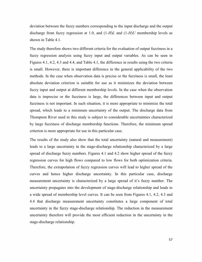
57

deviation between the fuzzy numbers corresponding to the input discharge and the output

discharge from fuzzy regression at 1.0, and (1-H)L and (1-H)U membership levels as

shown in Table 4.1.

The study therefore shows two different criteria for the evaluation of output fuzziness in a

fuzzy regression analysis using fuzzy input and output variables. As can be seen in

Figures 4.1, 4.2, 4.3 and 4.4, and Table 4.1, the difference in results using the two criteria

is small. However, there is important difference in the general applicability of the two

methods. In the case when observation data is precise or the fuzziness is small, the least

absolute deviation criterion is suitable for use as it minimizes the deviation between

fuzzy input and output at different membership levels. In the case when the observation

data is imprecise or the fuzziness is large, the differences between input and output

fuzziness is not important. In such situation, it is more appropriate to minimize the total

spread, which leads to a minimum uncertainty of the output. The discharge data from

Thompson River used in this study is subject to considerable uncertainties characterized

by large fuzziness of discharge membership functions. Therefore, the minimum spread

criterion is more appropriate for use in this particular case.

The results of the study also show that the total uncertainty (natural and measurement)

leads to a large uncertainty in the stage-discharge relationship characterized by a large

spread of discharge fuzzy numbers. Figures 4.1 and 4.2 show higher spread of the fuzzy

regression curves for high flows compared to low flows for both optimization criteria.

Therefore, the extrapolation of fuzzy regression curves will lead to higher spread of the

curves and hence higher discharge uncertainty. In this particular case, discharge

measurement uncertainty is characterized by a large spread of it’s fuzzy number. The

uncertainty propagates into the development of stage-discharge relationship and leads to

a wide spread of membership level curves. It can be seen from Figures 4.1, 4.2, 4.3 and

4.4 that discharge measurement uncertainty constitutes a large component of total

uncertainty in the fuzzy stage-discharge relationship. The reduction in the measurement

uncertainty therefore will provide the most efficient reduction in the uncertainty in the

stage-discharge relationship.

58

Table 4.1. Sensitivity of fuzzy discharge numbers to different degree of belief

Degree of belief Total spread (m3/s) Deviation (m

3/s)

H Min. Mean Max. Min. Mean Max.

Minimum spread criteria 0.5

0.7

0.9

266

189

156

1979

1405

1090

5471

3864

2989

0

0

0

70

71

73

375

378

382

Minimum deviation criteria 0.5

0.7

0.9

255

181

140

1997

1424

1105

5647

4018

3116

0

0

0

67

67

67

348

348

348

59

CHAPTER 5

Hysteresis analysis using fuzzified Jones formula

This chapter presents a methodology for an analysis of a looped rating curve using

fuzzified form of Jones formula. The methodology is based on consideration of

parameters of Jones formula as fuzzy numbers, whose spreads are determined using a

multi-objective optimization algorithm. The discharge and stage data from three stations

in the Chattahoochee River in Georgia, USA is used for the analysis.

5.1 Methodology for hysteresis analysis using fuzzified Jones formula

5.1.1 Derivation of Jones formula

The Jones formula is derived from one dimensional hydrodynamic model, which is based

on the conservation principles of mass and momentum, also known as the St. Venant

equations. The equations are expressed in terms of the continuity (equation 5.1) and the

momentum equations (equation 5.2):

0=∂∂

+∂∂

t

A

x

Q (5.1)

( ) 02

=−+∂∂

+

∂∂

+∂∂

of SSgAx

hgA

A

Q

xt

Q (5.2)

where, h = depth of flow [m], Q = discharge [m3/s], A = active cross sectional area of

flow [m2], g = gravitational acceleration [m/s

2], Sf = friction slope, S0 = bed slope, x =

distances along the channel [m] and t = time [s].

The momentum equation (5.2) can be rewritten as:

x

h

A

Q

xgAt

Q

gASS of ∂

∂−

∂∂

−∂∂

−=211

(5.3)

60

Neglecting the local acceleration t

Q

gA ∂∂1

and convective acceleration terms

∂∂

A

Q

xgA

21, equation (5.3) can be rewritten as diffusion wave equation:

x

hSS of ∂

∂−= (5.4)

The friction slope Sf and the bed slope So in the river channel can be evaluated in terms of

energy loss equations:

fSKQ = (5.5)

0SKQo = (5.6)

Where, K is the conveyance of the channel with same dimension as discharge [m3/s] and

Qo is the reference discharge assuming steady flow conditions. The conveyance is

assumed to be equal for both the unsteady discharge and steady discharge.

Combining equations (5.4), (5.5) and (5.6) leads to the equation:

2/1

11

∂∂

−=x

h

SQQ

o

o (5.7)

The longitudinal gradient of the water depth, x

h

∂∂

can be replaced by an alternative term

deducible from a flood record at a section as:

0=∂∂

+∂∂

t

h

x

hck (5.8)

where, ck = kinematic wave celerity [m/s] and t = time step [s].

Combining equations (5.7) and (5.8), we obtain the following equation which is also

referred to as the Jones formula:

2/1

11

∂∂

+=t

h

cSQQ

ko

o (5.9)

61

The kinematic wave celerity can be estimated using the following equation (Ponce 1989):

A

Qc o

k ∂∂

= (5.10)

This leads to a modified form of the Jones formula:

2/1

1

∂∂∂∂

+=

A

QS

t

h

QQo

o

o (5.11)

Therefore, in the Jones formula, the term under the square root modifies the steady state

discharge to looped form based on channel slope, kinematic wave celerity and rate of

change of stage. The bed slope in the channel can be estimated from the hydraulic data

and the water surface slope t

h

∂∂

can be obtained from the observed stage hydrograph. For

the calculation of the steady flow discharge Qo, the single value rating curve equation can

be used:

b

o ahQ = (5.12)

where, a and b are the coefficients of the relationship.

Combination of equations (5.11) and (5.12) leads to the following equation:

2/1

)(1

∂∂∂∂

+=

A

ahS

t

h

ahQb

o

b (5.13)

5.1.2 Fuzzification of Jones formula

A major source of uncertainty in the application of the Jones formula is a number of

simplifying assumptions, the equation is based upon. Some of the assumptions will never

be fully met in any natural river, and lead to unknown trade-off between model bias and

model simplicity (Petersen-Overleir 2006). The Jones formula also needs to be calibrated

with the measured discharge data. However, the discharge data consist considerable

uncertainty (Shrestha and Simonovic 2008a), which will also affect the simulation using

62

Jones formula. These uncertainties can be taken into account through fuzzification of

equation (5.13), by considering coefficients a and b as fuzzy numbers. In addition, the

bed slope So is also unknown and uncertain parameter, which can be expressed as a fuzzy

number. Since the term under the square root of the equation (5.13) modifies the steady

state discharge to a looped form, only the coefficients under the square root are

considered as fuzzy numbers in this work. The fuzzified form of equation (5.13) is:

2/1

ˆ)ˆ(ˆ

1

∂∂∂∂

+=

A

haS

t

h

ahQb

o

b (5.14)

5.1.3 Analysis of fuzzified Jones formula using fuzzy regression

The spreads of the fuzzy coefficients a and b can be evaluated using a fuzzy nonlinear

regression. More details on fuzzy regression methodology is given in chapters 1 and 4.

For a degree of belief H, the left and right spreads of the L-R fuzzy numbers a , b and oS


)1(ˆ)1( HmaHm aaaa −+≤≤−− βα (5.15)

)1(ˆ)1( HmbHm bbbb −+≤≤−− βα (5.16)

)1(ˆ)1( HmSHm SSoSS −+≤≤−− βα (5.17)

The fuzzified form of the Jones formula leads to a possible bounds of inner and outer

loops incorporating the observation points. Both the inner and outer loops consist of

rising and falling limbs. Accordingly, the discharge values of the inner loop should be

either less than or equal to the observations in the rising limb and equal to or greater than

the observations in the falling limb. Similarly, the discharge values of the outer loop

should be either greater than or equal to the observations in the rising limb and equal to

or less than the observations in the falling limb. Therefore the equations (8), (9a), (9b)

and (9c) are integrated in the following conditions:

Inner loop rising limb:

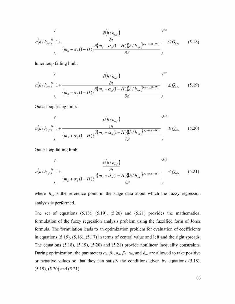
63

( )( )

{ } { }( ){ } obsHm

refaa

SS

ref

b

ref Q

A

hhHmHm

t

hh

hhabb

≤

∂

−−∂−−

∂

∂

+ −−

2/1

)1(/)1(

)1(

/

1/ ααα

(5.18)

Inner loop falling limb:

( )( )

{ } { }( ){ } obsHm

refaa

SS

ref

b

ref Q

A

hhHmHm

t

hh

hhabb

≥

∂

−−∂−−

∂

∂

+ −−

2/1

)1(/)1(

)1(

/

1/ ααα

(5.19)

Outer loop rising limb:

( )( )

{ } { }( ){ } obsHm

refaa

SS

ref

b

ref Q

A

hhHmHm

t

hh

hhabb

≥

∂

−+∂−+

∂

∂

+ −+

2/1

)1(/)1(

)1(

/

1/ ααα

(5.20)

Outer loop falling limb:

( )( )

{ } { }( ){ } obsHm

refaa

SS

ref

b

ref Q

A

hhHmHm

t

hh

hhabb

≤

∂

−+∂−+

∂

∂

+ −+

2/1

)1(/)1(

)1(

/

1/ ααα

(5.21)

where refh is the reference point in the stage data about which the fuzzy regression

analysis is performed.

The set of equations (5.18), (5.19), (5.20) and (5.21) provides the mathematical

formulation of the fuzzy regression analysis problem using the fuzzified form of Jones

formula. The formulation leads to an optimization problem for evaluation of coefficients

in equations (5.15), (5.16), (5.17) in terms of central value and left and the right spreads.

The equations (5.18), (5.19), (5.20) and (5.21) provide nonlinear inequality constraints.

During optimization, the parameters αa, βa, αb, βb, αS, and βS, are allowed to take positive

or negative values so that they can satisfy the conditions given by equations (5.18),

(5.19), (5.20) and (5.21).

64

For the evaluation of the spread of the loops a criteria based on minimization of the

spread (Wang and Tsaur 2000) of the loop is considered, which provides an objective

function for the optimization:

( )( )

{ }{ }( ){ }

( )( )

{ }{ }( ){ }

2/1

)1(

1

2/1

)1(

/)1()1(

/

1/

/)1()1(

/

1/

∂

−−∂−−

∂

∂

+

−

∂

−+∂−+

∂

∂

+

−−

=−+∑

A

hhHmHm

t

hh

hha

A

hhHmHm

t

hh

hha

Hm

refaa

SS

ref

b

ref

n

iHm

refaa

SS

ref

b

ref

bb

bb

α

α

αα

αα

(5.22)

where n is the number of observation data.

5.2 Case study: Application of fuzzified Jones formula for hysteresis analysis

We use the stage and discharge measurements at three stations in Chattahoochee River

reach from Georgia, USA (Faye and Cherry 1980) for the analysis of hysteresis using the

fuzzified Jones formula. River flow in this reach is predominantly controlled by the

Buford dam located upstream. The stage and discharge data in the river reach were

collected during the period of March 21-23, 1976, when the regulated discharge at

Buford dam was increased to about 8000 ft3/s (≈225 m

3/s). Continuous stage and

discharge measurements at 5 to 10 minutes interval were obtained at a number of stations

downstream of the dam using automatic digital recorders. For the measurement of

discharge, a minimum of 17 verticals were established across the river cross section at

each station. During the measurement each position was established sequentially and

flow depth, mean velocity, and time were recorded. Velocity area method was used to

calculate the total discharge for each measurement. A detailed description of the

discharge measurement in the Chattahoochee River is available in Faye and Cherry

(1980).

Petersen-Overleir (2006) used the Jones formula to reproduce rating curve hysteresis in

the Chattahoochee River. He used simplifying assumptions about the hydraulic and

65

geometric properties of the river channel and replaced physically based terms in the Jones

formula with parameters. Although a good reproduction of the hysteresis curve was

obtained, the use of non-physical parameters adds more uncertainty to the Jones formula.

Due to this reason, a new methodology is introduced in this paper.

We use a fuzzified form of the Jones formula to reproduce the hysteresis under various

sources of uncertainty. We use the data from the stations (i) Georgia Highway 141, (ii)

Littles Ferry Bridge and (iii) Georgia Highway 120 at the Chattahoochee River for the

analyses. Since the velocity area method is used for the aggregation of discharge, the

measurement data is affected by the uncertainties that we considered in our previous

work (Shrestha and Simonovic 2008a): (i) limited number of verticals; (ii) limited

number of points on a vertical; (iii) limited exposure time; (iv) current meter rating, (v)

depth measurement; and (vi) width measurement. However no specific information on

individual measurements of velocity, width and depth are available, so we did not

consider these uncertainties in this work.

The methodology used in this paper is based on the fuzzy nonlinear regression analysis

with parameters expressed as fuzzy numbers. We use two different curves meeting at a

point to represent the low and high flows in the steady flow equation (5.12). For

simplicity, we use symmetrical triangular L–R fuzzy numbers with equal left and right

spreads for the coefficients a , b and oS in equations (5.15), (5.16) and (5.17),

respectively. This reduces the decision variables for fuzzy regression to twelve,

consisting of six central values and six spreads (three each, for low and high flows). The

available measurement data is analyzed to determine an appropriate break point between

low and high flows and a reference point. For convenience, the brake point and reference

points are selected at the same stage for each of the stations. To capture uncertainties in

the measurement of discharge, we use a degree of belief H, which increases the spread of

the fuzzy regression curve and therefore spread of the output. Due to lack of information

on discharge measurement uncertainty, we use relatively low value of degree of belief of

0.5.

We initially used the sequential quadratic programming method (Fletcher 1987),

available in the MATLAB Optimization Toolbox (The MathWorks Inc. 2008) for the

66

optimization of the fuzzy regression equation. The equations (5.18), (5.19), (5.20) and

(5.21) are used as nonlinear inequality constraints and the equation (5.22) as the objective

function for the optimization. However, the use of equations (5.18), (5.19), (5.20) and

(5.21) as constraints which could not be violated (hard constraints) did not yield any

feasible solution for any of the these stations. We observed that a major problem in the

use of equations (5.18), (5.19), (5.20), (5.21) and (5.22) for optimization, is the square

root term in each of these equations. When the term under the square root becomes

negative, it gives an imaginary number output and optimization could not be completed

successfully.

To overcome this problem, we use an alternative strategy for optimization. Instead of

using equations (5.18), (5.19), (5.20) and (5.21) as hard constraints, they are considered

as soft constraints by allowing violations. The soft constraint is used as the objective

function to minimize the number of violations. For this purpose, we specified each

violation of the criteria as 1 and non-violation as 0, and expressed the sum of violation

and non-violation instances as the objective function. Therefore, we have two objective

functions for the evaluation of the coefficients of the fuzzified Jones formula: (i) criterion

provided by equation (11); and (ii) minimization of the violation of the constraints

provided by equations (5.18), (5.19), (5.20) and (5.21). In addition, the third objective

function is used to evaluate the ‘goodness of fit’ of the solution with membership level 1

with observations. For this evaluation, the criterion provided by the Nash-Sutcliffe

coefficient is used. Since the optimization problem is considered as a minimization

problem, we use the Nash-Sutcliffe coefficient of efficiency subtracted from unity.

( )

( )∑

∑

=

=

−

−

=−n

j

obsobsj

n

j

simjobsj

QQ

QQ

NSCE

1

2

,

1

2

,,

1 (5.23)

where, NSCE is the Nash-Sutcliffe coefficient of efficiency, n is the number of

observations, Qj,obs is the observed discharge and Qj,sim is the simulated discharge for

membership level 1 of fuzzified Jones formula at time step j. obs

Q is the mean of the

observed discharge.

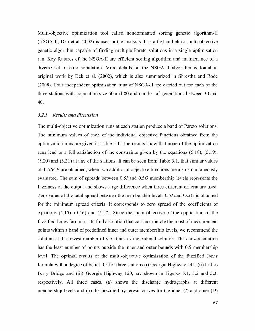
67

Multi-objective optimization tool called nondominated sorting genetic algorithm-II

(NSGA-II; Deb et al. 2002) is used in the analysis. It is a fast and elitist multi-objective

genetic algorithm capable of finding multiple Pareto solutions in a single optimisation

run. Key features of the NSGA-II are efficient sorting algorithm and maintenance of a

diverse set of elite population. More details on the NSGA-II algorithm is found in

original work by Deb et al. (2002), which is also summarized in Shrestha and Rode

(2008). Four independent optimisation runs of NSGA-II are carried out for each of the

three stations with population size 60 and 80 and number of generations between 30 and

40.


The multi-objective optimization runs at each station produce a band of Pareto solutions.

The minimum values of each of the individual objective functions obtained from the

optimization runs are given in Table 5.1. The results show that none of the optimization

runs lead to a full satisfaction of the constraints given by the equations (5.18), (5.19),

(5.20) and (5.21) at any of the stations. It can be seen from Table 5.1, that similar values

of 1-NSCE are obtained, when two additional objective functions are also simultaneously

evaluated. The sum of spreads between 0.5I and 0.5O membership levels represents the

fuzziness of the output and shows large difference when three different criteria are used.

Zero value of the total spread between the membership levels 0.5I and O.5O is obtained

for the minimum spread criteria. It corresponds to zero spread of the coefficients of

equations (5.15), (5.16) and (5.17). Since the main objective of the application of the

fuzzified Jones formula is to find a solution that can incorporate the most of measurement

points within a band of predefined inner and outer membership levels, we recommend the

solution at the lowest number of violations as the optimal solution. The chosen solution

has the least number of points outside the inner and outer bounds with 0.5 membership

level. The optimal results of the multi-objective optimization of the fuzzified Jones

formula with a degree of belief 0.5 for three stations (i) Georgia Highway 141, (ii) Littles

Ferry Bridge and (iii) Georgia Highway 120, are shown in Figures 5.1, 5.2 and 5.3,

respectively. All three cases, (a) shows the discharge hydrographs at different

membership levels and (b) the fuzzified hysteresis curves for the inner (I) and outer (O)

68

bounds at membership level 0.5. Therefore, the curves between 0.5I and 0.5O represent

the combined uncertainty in measurement data and simplification of the unsteady flow

equations using Jones formula.

The results of the study show that discharge values are higher at the outer membership

level in comparison to the inner membership level at the rising limb. In the case of falling

limb, discharge values are higher at the inner membership level in comparison to the

outer membership level. The results also show that a large spreads of coefficients of

fuzzified Jones formula is necessary in order to represent the dynamics of the measured

data. It may be possible to obtain a smaller spread if the inner and outer loops are

optimized separately. However, the optimization of the outer and inner membership

levels together with fuzzy regression enables the evaluation of the not only the bounds,

but also different membership levels inside or outside the bounds.

Table 5.1. Performance of the multi-objective optimization runs at three station

Station Criteria Sum of spreads

bet. 0.5I & 0.5O

memb. levels

No. of

violations of

constraints

Nash-Sutcliffe

coefficient

(1-NSCE)

Georgia

Highway 141

Min. spread

Min. no. of violations

Min. 1-NSCE

0

3865

2179

144

6

32

0.007

0.009

0.004

Littles Ferry

Bridge

Min. spread


Min. 1-NSCE

0

2877

3434

151

3

20

0.006

0.006

0.005

Georgia

Highway 120

Min. spread


Min. 1-NSCE

0

2167

1638

155

14

66

0.006

0.007

0.006

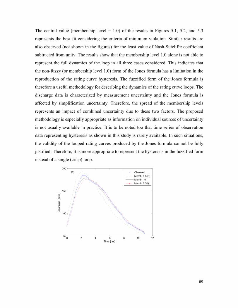
69

The central value (membership level = 1.0) of the results in Figures 5.1, 5.2, and 5.3

represents the best fit considering the criteria of minimum violation. Similar results are

also observed (not shown in the figures) for the least value of Nash-Sutcliffe coefficient

subtracted from unity. The results show that the membership level 1.0 alone is not able to

represent the full dynamics of the loop in all three cases considered. This indicates that

the non-fuzzy (or membership level 1.0) form of the Jones formula has a limitation in the

reproduction of the rating curve hysteresis. The fuzzified form of the Jones formula is

therefore a useful methodology for describing the dynamics of the rating curve loops. The

discharge data is characterized by measurement uncertainty and the Jones formula is

affected by simplification uncertainty. Therefore, the spread of the membership levels

represents an impact of combined uncertainty due to these two factors. The proposed

methodology is especially appropriate as information on individual sources of uncertainty

is not usually available in practice. It is to be noted too that time series of observation

data representing hysteresis as shown in this study is rarely available. In such situations,

the validity of the looped rating curves produced by the Jones formula cannot be fully

justified. Therefore, it is more appropriate to represent the hysteresis in the fuzzified form

instead of a single (crisp) loop.

0 2 4 6 8 10 1250

100

150

200

Time [hrs]

Dis

charg

e [m

3/s

]

Observed

Memb. 0.5(O)

Memb 1.0

Memb. 0.5(I)

(a)

70

50 100 150 200

6

6.2

6.4

6.6

6.8

7

7.2

7.4

Discharge [m3/s]

Sta

ge [m

]

Observed

Memb. 0.5(O)

Memb. 1

Memb. 0.5(I)

(b)

Figure 5.1. Results of the fuzzified Jones formula at Georgia Highway 141 station at

different membership levels: (a) discharge hydrograph, (b) looped rating curve

0 2 4 6 8 10 12 140

50

100

150

200

250

Time [hrs]

Dis

charg

e [m

3/s

]

Observed

Memb. 0.5(O)

Memb. 1.0

Memb. 0.5(I)

(a)

71

0 50 100 150 200 2505

5.5

6

6.5

7

7.5

8

8.5

Discharge [m3/s]

Sta

ge [m

]

Observed

Memb. 0.5(O)

Memb. 1.0

Memb. 0.5(I)

(b)

Figure 5.2. Results of the fuzzified Jones formula at Littles Ferry Bridge station at


0 2 4 6 8 10 12 1420

40

60

80

100

120

140

160

180

200

220

Time [hrs]

Dis

charg

e [m

3/s

]

Observed

Memb. 0.5(O)

Memb. 1.0

Memb. 0.5(I)

(a)

72

20 40 60 80 100 120 140 160 180 200 2205

5.5

6

6.5

7

7.5

Discharge [m3/s]

Sta

ge [m

]

Observed

Memb. 0.5(O)

Memb. 1.0

Memb. 0.5(I)

(b)

Figure 5.3. Results of the fuzzified Jones formula at Georgia Highway 120 station at


73

CHAPTER 6

Conclusions and Recommendations

Discharge records are essential for hydrologic and hydraulic analyses of river systems.

The primary purpose of a gauging station is to provide discharge records, usually by

measuring a stage and converting it to discharge by means of a stage-discharge

relationship. However, there are inherent uncertainties in measurement of stage and

discharge values and derivation of the stage-discharge relationship. In general, the

measurement uncertainty arises due to (i) random and systematic errors in measurement

instrumentation; and (ii) approximation of velocity distribution and channel geometry

with a finite number of measurements. On the other hand, the stage-discharge

relationship is affected by natural uncertainties due to unsteady flow in the river and

changes in measurement cross section. Due to unsteady flow, the stage-discharge

relationship takes a loop form, referred to as hysteresis, which makes the hypothesis of

single valued stage-discharge relationship incompatible. Another source of natural

uncertainty is change in river cross section due to physical processes of erosion and

sedimentation. Discharge and stage measurements are made over a period of time,

usually over a few years. If the change in the cross section is not taken into account, it

introduces systematic error or bias in the regression data and affects the rating curve

established using the regression analysis.

For the quantification of stage-discharge measurement uncertainties, the International

Organization for Standardization (ISO-748) suggests the range of values at 95%

confidence level for different sources of uncertainty. This recommendation is based on

investigations carried out since 1968. The ISO-748 recommends independent

determination of uncertainty in each measurement for the application to a particular case

study. However, in most cases, independent value of confidence interval in the

measurement is not available, which limits the applicability of statistical quantification of

the uncertainties. It is to be noted too that randomness is not the only source of

74

uncertainty in discharge measurements as they can also be affected by systematic

uncertainty, human error and other subjective uncertainties. These uncertainties due to

bias, non-uniqueness and simplification in the stage-discharge relationship cannot be

directly expressed in the statistical framework using confidence intervals.

The fuzzy set theory-based approach is explored in this report as an alternative way of

analyzing various uncertainties associated with measurements and the rating curve. The

fuzzy approach provides a non-probabilistic framework for representation of

uncertainties using vaguely defined boundaries of fuzzy sets. The method is used for

quantification and aggregation of individual sources of uncertainty in discharge

measurement and definition of uncertainty in the stage discharge relationship.

In the first part of this report, an original fuzzy set theory based approach is used for the

consideration of different sources of uncertainty in measurement of stage and discharge

and their aggregation into a combined uncertainty. Each of the measurement quantities is

represented as a triangular fuzzy number with the spread determined on the basis of the

ISO-748 guidelines. The extension principle based fuzzy arithmetic is used for the

aggregation of different uncertainties and calculation of the total measurement

uncertainty. The results of the study are compared with the fuzzified form of ISO-748

formulation for the calculation of combined measurement uncertainty. The results of the

Spences bridge location on the Thompson river in British Columbia, Canada show high

uncertainty in the measurement of the discharge (expressed by the wide support of the

discharge fuzzy number). The analysis of different uncertainty sources shows that the

number of points on a vertical for the measurement of velocity is the largest source of

uncertainty in the discharge measurement. Therefore, increase in the number of points on

a vertical results in the largest reduction in the measurement uncertainty. Number of

verticals in a cross section is another important source of uncertainty in discharge

measurement. Although there is a limited reduction in uncertainty when the number of

verticals is increased beyond 25, there will be a considerable increase in uncertainty when

the number of verticals is reduced below 10. These results can be used as a basis for the

improvement in the measurement methods and subsequent reduction in the stage

discharge measurement uncertainties.

75

The study also presents a methodology for handling overall random uncertainties in the

Acoustic Doppler current profiler discharge measurement. The results show that the

ADCP discharge measurement uncertainty is very small compared to total uncertainty

using current meter measurement. Although the uncertainties in the ADCP does not

incorporate different sources of possible uncertainties, it can still be expected that the

total uncertainty in the measurement will still remain small compared to the current meter

discharge measurement uncertainty. The method can be adapted to quantify individual

random uncertainties as well as systematic uncertainties.

The second part of the report builds on the results of quantification of uncertainties at

Spences bridge location on the Thompson river. Based on the representation of discharge

and stage measurement uncertainties using fuzzy numbers, the uncertainties in the stage-

discharge relationship is analyzed using fuzzy regression. The methodology is based on

the fuzzy nonlinear regression analysis with the input and output variables as well as the

coefficients of the stage-discharge relationship expressed as fuzzy numbers. Therefore,

the method takes into account the fuzziness in the input and output variables as well as

the coefficients of the relationship. Two different criteria are used for an optimal

evaluation of the output fuzziness: minimum spread and least absolute deviation criteria.

The fuzzy nonlinear regression analysis leads to a definition of lower and upper

uncertainty bounds on the stage-discharge relationship. The use of two optimization

criteria for the evaluation of the output fuzziness leads to similar results with lower

spread in the case of minimum spread criteria and the lower deviation between the fuzzy

numbers of the input discharge and output discharge from fuzzy regression at different

membership levels.

In this particular case study, the discharge measurement uncertainty is characterized by a

large spread of its fuzzy number. The uncertainty propagates into the stage-discharge

relationship and leads to a wide spread of the membership level curves. The reduction in

the measurement uncertainty therefore will provide the most efficient reduction in the

uncertainty in the stage-discharge relationship.

The third part of this reports deals with fuzzified form of Jones formula for the treatment

of uncertainties in a looped rating curve using data from three stations in the

76

Chattahoochee River in Georgia, USA. The Jones formula is one of the methods used for

the analysis of looped rating curves. However, it is subject to uncertainty arising from the

simplification of unsteady flow equation. There are also additional uncertainties in the

application of the Jones formula as discharge values used for fitting the formula are

affected by the measurement uncertainties. Based on the representation of coefficients of

Jones formula as fuzzy numbers, the uncertainties in the looped stage-discharge

relationship are defined using an optimization scheme. A multi-objective optimization

scheme NSGA-II is used for the evaluation of the output fuzziness. The measurement

data from three stations in the Chattahoochee River in Georgia, USA is used for the

analyses.

The multi-objective optimization scheme leads to a definition of the inner and the outer

uncertainty bounds on the looped stage-discharge relationship. From the Pareto solutions

obtained from the multi-objective optimization runs, a solution which has the most

number of observation points inside the inner and outer loops as the optimal solutions is

selected. The fuzzified form of Jones formula is able to represent the dynamics of

hysteresis loop, which gives an estimation of the combined uncertainty, due to discharge

measurement errors and simplification of the unsteady flow equations. It is to be noted

that time series of observation data representing hysteresis is rarely available. Due to this

reason, the validity of the looped rating curves produced by the non-fuzzy Jones formula

cannot be fully justified and it is therefore recommended to represent the hysteresis in the

fuzzified form.

The study has therefore demonstrated that the fuzzy set theory-based approach is an

effective means of treating uncertainties in stage-discharge measurement and the rating

curves in a non-probabilistic framework. The method considers uncertainties using

vaguely defined boundaries of fuzzy sets and can incorporate different sources of

uncertainty arising from random and systematic errors. The method allows quantification

and aggregation of individual sources of uncertainty in discharge measurement and

definition of uncertainty in the stage discharge relationship. Moreover, the method allows

assessment of random and systematic uncertainties in the measurement and indirect

consideration of uncertainties due to hysteresis and changes of river cross section. The

77

method also allows the treatment of classical methods such as Jones formula in a

fuzzified form, which leads to a representation of dynamics of looped rating. For most

gauging stations, confidence levels of different uncertainty sources are usually

unavailable for a probabilistic consideration of uncertainties. In these situations, the fuzzy

set theory is recommended to be used as an alternative methodology.

78

ACKNOWLEDGEMENTS

The authors would like to acknowledge the financial support of the National Science and

Engineering Research Council of Canada. We thank Mr. David Hutchinson M.Sc. of

Environment Canada (Vancouver), Mr. Guy Morin of Environment Canada (Montreal)

and Dr. Asgeir Petersen-Øverleir of the Department of Hydrology, Norway for providing

data used in this study.

79

REFERENCES

Bárdossy, A., Bogardi, I. and Duckstein, L. (1990). Fuzzy regression in hydrology. Water

Resources Research 26(7), 1497–1508.

Chang, Y. H. O. and Ayyub, B. M., (2001). Fuzzy regression methods - a comparative

assessment. Fuzzy Sets and Systems 119(2), 187-203.

Choi, S. H. and Buckley, J. J. (2008). Fuzzy regression using least absolute deviation

estimators. Soft Computing 12, 257-263.

Chow, V. T., Maidment, D. R. and Mays, L. W. (1988). Applied Hydrology. McGraw

Hill Inc., Singapore.

Clarke, R.T. (1999). Uncertainty in the estimation of mean annual flood due to rating-

curve indefinition. Journal of Hydrology 222(1/4), 185–190.

Clemmens, A.J., and Wahlin, B.T. (2006). Accuracy of annual volume from current-

meter-based stage discharges. Journal of Hydrologic Engineering-ASCE 11(5),

489-501.

Cunge, J. A. Holly, F. M. and Verway, A. (1980). Practical Aspects of Computational

River Hydraulics. Pitman, London, UK.

Deb, K., Pratap, A., Agarwal, S., and Meyarivan, T., (2002). A fast and elitist

multiobjective genetic algorithm, NSGA-II. IEEE Transactions on Evolutionary

Computation 6(2), 188-197.

Dubois, D. and Prade, H. (1980). Fuzzy Sets and Systems, Theory and Applications.

Academic Press Inc., New York, USA.

D'Urso, P. (2003). Linear regression analysis for fuzzy/crisp input and fuzzy/crisp output

data. Computational Statistics and Data Analysis 42(1-2), 47-72.

El-Baroudy, I. and Simonovic, S. (2006). Application of the fuzzy performance measures

to the City of London water supply system. Canadian Journal of Civil Engineering

33, 255–265.

Faye, R. E. and Cherry, R. N. (1980). Channel and dynamic flow characteristics of the

Chattahoochee River, Buford Dam to Georgia Highway 141. US Geological

Survey Water Supply Paper 2063.

80

Ferrero, A. and Salicone, S. (2003). An innovative approach to the determination of

uncertainty in measurements based on fuzzy variables. IEEE Transactions on

Instrumentation and Measurement 52(4), 1174-1181.

Ferrero, A. and Salicone, S. (2004). The random-fuzzy variables, A new approach to the

expression of uncertainty in measurement. IEEE Transactions on Instrumentation

and Measurement 53(5), 1370-1377.

Fletcher, R. (1987). Practical Methods of Optimization. 2nd ed., John Wiley and Sons,

Chichester.

Gonzalez-Castro, J. and Muste, M. (2007). Framework for Estimating Uncertainty of

ADCP Measurements from a Moving Boat Using Standardized Uncertainty

Analysis,” Journal of Hydraulic Engineeringg-ASCE 133(12), 1390-1411.

Guyonnet, D., Bourgine, B., Dubois, D., Fargier, H., Come, B. and Chiles, J.P. (2003).

Hybrid approach for addressing uncertainty in risk assessments. Journal of

Environmental Engineering-ASCE 129(1), 68-78.

Henderson F. M. (1966). Open Channel Flow. Macmillan, New York.

Herschy, R. W. (1995). Streamflow Measurement, second edition, E and FN, Chapman

and Hall.

Herschy, R. W. (1999). Flow measurement. In Hydrometry Principles and Practices,

Edited by R. W. Herschy, John Wiley and Sons Ltd., Chichester, UK. 9–84.

ISO-748 (1997). Measurement of liquid flow in open channels-velocity area methods.

International Organization for Standardization, Geneva. 41 p.

ISO 1100-2 (1998). Measurement of liquid flow in open channels -- Part 2,

Determination of the stage-discharge relation, International Organization for

Standardization, Geneva. 25 p.

ISO (1993). Guide to the Expression of Uncertainty in Measurement, International

Organization for Standardization, Geneva. 99 p

ISO/TR-5168 (1998). Measurement of fluid flow - Evaluation of uncertainties.

International Organization for Standardization, Geneva. 78 p.

Jones, B. E. (1916). A method of correcting river discharge for a changing stage. US

Geological Survey Water Supply Paper 375-E.

81

Kao, C. and Chyu, C. L. (2003). Least-squares estimates in fuzzy regression analysis.

European Journal of Operational Research 148(2), 426-435.

Klir, G. J. (1997). Fuzzy arithmetic with requisite constraints. Fuzzy Sets and Systems

91(2), 165-175.

Lee, Y. W., Chung, S. Y., Bogardi, I., Dahab, M. F. and Oh, S. E. (2001). “Dose–

response assessment by a fuzzy linear regression method.” Water Science and

Technology 43(2), 133–140.

Mauris, G., Lasserre, V., and Foulloy, L. (2001). A fuzzy approach for the expression of

uncertainty in measurement. Measurement 29(3), 165-177.

Mousavi, S.J., Ponnambalam, K. and Karray, F. (2007). Inferring operating rules for

reservoir operations using fuzzy regression and ANFIS. Fuzzy Sets and Systems

158(10), 1064-1082.

Muste, M., Yu, K., Pratt, T., and Abraham, D. (2004a). Practical aspects of ADCP data

use for quantification of mean river flow characteristics, Part 1 moving-vessel

measurements, Flow Measurement and Instrumentation 15(1), 1-16.

Muste, M., Yu, K., Pratt, T. and Abraham, D. (2004b). Practical aspects of ADCP data

use for quantification of mean river flow characteristics, Part 11 Fixed- vessel

measurements, Flow Measurement and Instrumentation 15(1), 17-28.

Pappenberger, F., Matgen, P., Beven, K.J., Henry, J. B., Pfister, L. and Fraipont de, P.

(2006). Influence of uncertain boundary conditions and model structure on flood

inundation predictions. Advances in Water Resources 29(10), 1430-1449.

Parodi, U. and Ferraris, L. (2004). Influence of stage discharge relationship on the annual

maximum discharge statistics. Natural Hazards 31(3), 603-611

Pelletier, P. M. (1988). Uncertainties in the single determination of river discharge, a

literature review. Canadian Journal of Civil Engineering 15(5), 834-850.

Petersen-Overleir, A. (2006). Modelling stage-discharge relationships affected by

hysteresis using the Jones formula and nonlinear regression. Hydrological

Sciences Journal, 51(3), 365-388.

Ponce V. M. (1989). Engineering Hydrology, Principles and Practices. Prentice Hall,

Englewood Cliffs, NJ.

82

Rantz, S. E. and others. (1982). Measurement and Computation of Streamflow, Vols. 1

and 2. U.S. Geological Survey Water-Supply Paper 2175.

Rehmel, M. (2007). Application of acoustic Doppler velocimeters for streamflow

measurements. Journal of Hydraulic Engineering-ASCE 133(12), 1433-1438.

Salicone, S. (2007). Fuzzy Variables and Measurement Uncertainty. In Measurement

Uncertainty an Approach via the Mathematical Theory of Evidence, Springer US,

15-29.

Samuels, P. G., Bramley, M. E., and Evans, E. P. (2002). Reducing uncertainty in

conveyance estimation. Proc., River Flow 2002 – International Conference on

Fluvial Hydraulics, D. Bousmar, and Y. Zech, eds, Swets & Zeitlinger, Lisse,

Netherlands.

Sauer, V. B., and Meyer, R. W. (1992). Determination of error in individual discharge

measurements, USGS Open-File Rep. No. 92-144, U.S. Geological Survey,

Norcross, Georgia.

Schmidt, A. R. (2002). Analysis of stage-discharge relations for open-channel flows and

their associated uncertainties, PhD Thesis, University of Illinois at Urbana-

Champaign, Department of Civil and Environmental Engineering. 349 p.

Shrestha, R. R. and Rode, M. (2008). Multi-objective calibration and fuzzy preference

selection of a distributed hydrological model, Environmental Modelling and

Software, 239(12), 1384-1395.

Shrestha, R. R. and Simonovic, S. P. (2008a). A fuzzy set theory based methodology for

analysis of measurement uncertainties in river discharge and stage, Submitted to

Canadian Journal of Civil Engineering.

Shrestha, R. R. and Simonovic, S. P. (2008b). Fuzzy nonlinear regression approach to

stage-discharge analyses, Submitted to Journal of Hydrologic Engineering-ASCE.

Shrestha, R. R. and Simonovic, S. P. (2008c). Analysis of hysteresis in stage-discharge

relationship using fuzzified Jones formula, Submitted to Advances in Water

Resources.

83

Shrestha, R. R., Bardossy, A. and Nestmann, F. (2007). Analysis and propagation of

uncertainties due to the stage-discharge relationship, a fuzzy set approach.

Hydrological Sciences Journal, 52(4), 595-610.

Simonovic, S. P. (2008). Managing Water Resources, Methods and Tools for a Systems

Approach, UNESCO, Paris and Earthscan James and James, London (in print),

Chapter 6, 129 p.

Simpson, M. R. (2001). Discharge measurements using a broad-band acoustic Doppler

current profiler, U.S. Geological Survey Open-File Report 01-1.

Tanaka, H., Uegima, S. and Asai, K. (1982). Linear regression analysis with fuzzy model.

IEEE Transactions on System Man and Cybernetics 12, 903–907

Terzi, R. A. (1981). Hydromeric Field Manual-Measurement of Streamflow,

Environment Canada, Inland Waters Directorate, Water Resources Branch, Ottawa,

Ontario.

The MathWorks Inc. (2008). Optimization Toolbox for use with MATLAB, Online

documentation, http,//www.mathworks.com/access/helpdesk/help/toolbox/optim.

Urbanski, M. K., and Wasowski, J. (2003). Fuzzy approach to the theory of measurement

inexactness. Measurement 34(1), 67-74.

USACE (1993). Engineering and Design, River Hydraulics, Engineer Manual 1110-2-

1416, US Army Corps of Engineers (USACE), Washington DC.

Wang, H. F. and Tsaur, R. C. (2000). Insight of a fuzzy regression model. Fuzzy Sets and

Systems 112(3), 355-369.

Whalley, N., Iredale, R. S., and Clare, A. F. (2001). Reliability and uncertainty in flow

measurement techniques - Some current thinking. Physics and Chemistry of the

Earth Part C-Solar-Terrestial and Planetary Science 26(10-12), 743-749.

WMO (2008). Assessment of the performance of flow measurement instruments and

techniques. Progress report,

http://www.wmo.ch/pages/prog/hwrp/FlowMeasurement.html

Wu, H. C. (2003). Linear regression analysis for fuzzy input and output data using the

extension principle. Computers and Mathematics with Applications 45(12), 1849-

1859.

84

Xia, X., Wang, Z. and Gao, Y. (2000). Estimation of non-statistical uncertainty using

fuzzy-set theory. Measurement Science and Technology, 11, 430–435.

Zadeh, L. A. (1965). Fuzzy sets. Information and Control 8, 338–353.

85

APPENDIX 1

Matlab source code

1a: Discharge uncertainty calculation using fuzzy arithmetic

fuz_arith_q.m function q_res=fuz_arith_q() % Calculation of the discharge uncertainties considering the individual % uncertainties in the measurement of each of the quantities % Each of the quantities: velocity, depth and width are considered as % fuzzy numbers and total uncertainty is calculated using fuzzy % arithmetic % load the data with first column id second width, third depth and the % fourth velocity load q_data.txt; [m1,m2]=size(q_data); % alpha cut of fuzzy number % alpha cut intervals alpha=0.1; a=[-1:alpha:1];a1=length(a); % tot_fuz1=zeros(a1,1); % define the id id=q_data(1); q_res=zeros(1,a1+1); j=0; while id<=q_data(m1); [R,C] = find(q_data==id); % Check whether the id number exist if (~isempty(R)); j=j+1; n=sum(C); % select the data with the same id qdat0=q_data(R(1):R(n),2:4); % sort the rows in ascending order with distance qdat1=sortrows(qdat0,1); % Discharge calculation using mid-section method % The area between the first and second, and second last and last verticals % are neglected

86

% Define the Width measurement (b(j+1)-b(j-1))/2 b3=qdat1(3:n,1); b1=qdat1(1:n-2,1); b=(b3-b1)/2; qdat=[b qdat1(2:n-1,2:3)]; % Define uncertainties in % and increase the 95% confidence interval value % by 50% to cover 99.7% (within three standard deviations) f=1.5; % Interpolate uncertainties according to the no of verticals xm=vert_uncert(n);xm1=xm*f; % width measurment (range of width between 0 to 100 m) xb=0.3;xb1=xb*f; % Depth measurement (sounding rod?) xd=0.7;xd1=xd*f; % Velocity measurement depends upon the actual velocity % one point method is used which has uncertainties as high as 15%! xp=15;xp1=xp*f; % current meter rating (individual rating is used) xc=1;xc1=xc*f; % time of exposure (for exposure time 1 min and velocity > 1 m. xe=6;xe1=xe*f; % Total uncertainties in the velocity measurement is calculated as the % square root of the sum of squares of all the uncertainties in velocity % measurement xv1=sqrt(xp1^2+xc1^2+xe1^2); % fuzzify % first column width width_fuz=fuzzify(qdat(:,1),xb1,alpha,'percent'); % second column depth depth_fuz=fuzzify(qdat(:,2),xd1,alpha,'percent'); % third column velocity vel_fuz=fuzzify(qdat(:,3),xv1,alpha,'percent'); % do an element wise multiplication to calculate partial fuzzy discharge % between the verticals q_fuz=width_fuz.*depth_fuz.*vel_fuz; % calculate the total fuzzy discharge Q_fuz=sum(q_fuz); % Multiply by uncertainties due to number of verticals % first fuzzify the uncertainties vert_fuz=fuzzify(0,xm1,alpha,'zero'); % Calculate the total fuzzy discharge Q_dis=(1+vert_fuz).*Q_fuz; % negative values for negative alpha level % k=1; % while k<=a1; % if a(k)<0;

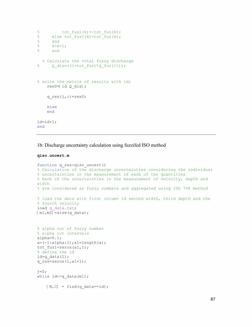
87

% tot_fuz1(k)=-tot_fuz(k); % else tot_fuz1(k)=tot_fuz(k); % end % k=k+1; % end % Calculate the total fuzzy discharge % Q_dis=((1+tot_fuz)*Q_fuz(11)); % write the matrix of results with id; res0=[id Q_dis]; q_res(j,:)=res0; else end id=id+1; end

1b: Discharge uncertainty calculation using fuzzifed ISO method

qiso.uncert.m function q_res=qiso_uncert() % Calculation of the discharge uncertainties considering the individual % uncertainties in the measurement of each of the quantities % Each of the uncertainties in the measurement of velocity, depth and width % are considered as fuzzy numbers and aggregated using ISO 748 method % load the data with first column id second width, third depth and the % fourth velocity load q_data.txt; [m1,m2]=size(q_data); % alpha cut of fuzzy number % alpha cut intervals alpha=0.1; a=(-1:alpha:1);a1=length(a); tot_fuz1=zeros(a1,1); % define the id id=q_data(1); q_res=zeros(1,a1+1); j=0; while id<=q_data(m1); [R,C] = find(q_data==id);

88

% Check whether the id number exist if (~isempty(R)); j=j+1; n=sum(C); % select the data with the same id qdat0=q_data(R(1):R(n),2:4); % sort the rows in ascending order with distance qdat1=sortrows(qdat0,1); % Discharge calculation using mid-section method % The area between the first and second, and second last and last verticals % are neglected % Define the Width measurement (b(j+1)-b(j-1))/2 b3=qdat1(3:n,1); b1=qdat1(1:n-2,1); b=(b3-b1)/2; qdat=[b qdat1(2:n-1,2:3)]; % calculate the partial discharge between the verticals par_dis=qdat(:,1).*qdat(:,2).*qdat(:,3); % sq_dis=par_dis.^2; tot_dis=sum(par_dis); % Define uncertainties in % and increase the 95% confidence interval value % by 50% to cover 99.7% (within three standard deviations) f=1.50; % Interpolate uncertainties according to the no of verticals xm=vert_uncert(n);xm1=xm*f; % width measurment (range of width between 0 to 100 m) xb=0.3;xb1=xb*f; % Depth measurement (sounding rod?) xd=0.7;xd1=xd*f; % Velocity measurement depends upon the actual velocity % one point method is used which has uncertainties as high as 15%! xp=15;xp1=xp*f; % current meter rating (individual rating is used) xc=1;xc1=xc*f; % time of exposure (for exposure time 1 min and velocity > 1 m. xe=6;xe1=xe*f; % fuzzify and calculate the square of the uncertainty values % width width_fuz=fuzzify(0,xb1,alpha,'zero'); % depth depth_fuz=fuzzify(0,xd1,alpha,'zero'); % velocity on of points in a vertical velp_fuz=fuzzify(0,xp1,alpha,'zero'); % current meter rating velc_fuz=fuzzify(0,xc1,alpha,'zero'); % time of exposure

89

vele_fuz=fuzzify(0,xe1,alpha,'zero'); % Uncertainties due to limited no of verticals vert_fuz=fuzzify(0,xm1,alpha,'zero'); % do element wise multiplication (square) of the fuzzified uncertainties % (except, no of verticals) com_fuz=width_fuz.^2+depth_fuz.^2+velp_fuz.^2+velc_fuz.^2+vele_fuz.^2; % multiply the square area with the com_fuzzy i=1; temp=zeros(n-2,a1); while i<n-2; temp(i,:)=par_dis(i)*sqrt(com_fuz); i=i+1; end % calculate the total uncertainties tot_fuz=sqrt(vert_fuz.^2+(sum(temp)/tot_dis).^2); % negative values for negative alpha level k=1; while k<=a1; if a(k)<0; tot_fuz1(k)=-tot_fuz(k); else tot_fuz1(k)=tot_fuz(k); end k=k+1; end % Calculate the total fuzzy discharge Q_fuz=((1+tot_fuz1)*tot_dis)'; % write the matrix of results with id; res0=[id Q_fuz]; q_res(j,:)=res0; else end id=id+1; end

1c: Stage uncertainty calculation using fuzzy arithmetic

fuz_arith_h.m

function h_res=fuz_arith_h()

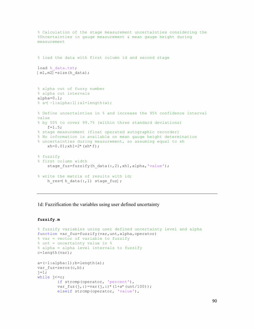
90

% Calculation of the stage measurement uncertainties considering the %Uncertainties in gauge measurement & mean gauge height during measurement % load the data with first column id and second stage load h_data.txt; [m1,m2]=size(h_data); % alpha cut of fuzzy number % alpha cut intervals alpha=0.1; % a=[-1:alpha:1];a1=length(a); % Define uncertainties in % and increase the 95% confidence interval value % by 50% to cover 99.7% (within three standard deviations) f=1.5; % stage measurement (float operated autographic recorder) % No information is available on mean gauge height determination % uncertainties during measurement, so assuming equal to xh xh=0.01;xh1=2*(xh*f); % fuzzify % first column width stage_fuz=fuzzify(h_data(:,2),xh1,alpha,'value'); % write the matrix of results with id; h_res=[h_data(:,1) stage_fuz];

1d: Fuzzification the variables using user defined uncertainty

fuzzify.m

% fuzzify variables using user defined uncertainty level and alpha function var_fuz=fuzzify(var,unt,alpha,operator) % var = vector of variable to fuzzify % unt = uncertainty value in % % alpha = alpha level intervals to fuzzify c=length(var); a=(-1:alpha:1);b=length(a); var_fuz=zeros(c,b); j=1; while j<=c; if strcmp(operator, 'percent'), var_fuz(j,:)=var(j,:)*(1+a*(unt/100)); elseif strcmp(operator, 'value'),

91

var_fuz(j,:)=var(j,:)+a*unt; elseif strcmp(operator, 'zero') var_fuz(j,:)=0+a*(unt/100); else end j=j+1; end

1e: Interpolation of uncertainties due to number of verticals

Vert_uncert.m function xm=vert_uncert(vert_num) % Interpolate uncertainties due to number of verticals xy=[5 15; 10 9; 15 6; 20 5; 25 4; 30 3; 35 2; 40 2; 45 2]; x=xy(:,1); y=xy(:,2); xm=interp1(x,y,vert_num);

1f: Fuzzy regression of fuzzy stage and discharge values with minimum distance criteria

f_regression_mindist.m function [b,fval] = f_regression_mindist() % This code requires MATLAB optimization toolbox! % The code generates lower and upper membership bounds of the stage % discharge relationship curves with both stage and discharge (variables) % treated as fuzzy numbers. % It generates fuzzy parameters of the stage discharge relationship % Degree of belief dob = 0.5; % Initialize shared variable % load the data hq_fuz=load('hq_fuz.txt'); hqdat=sortrows(hq_fuz,6); % Scale the data and devide the reference point

92

h11=(hqdat(1:28,5)+1)/3.36;h21=(hqdat(1:28,6)+1)/3.36;h31=(hqdat(1:28,7)+1)/3.36; h117=(h21-(h21-h11)*dob);h317=(h21+(h31-h21)*dob); h12=(hqdat(28:56,5)+1)/3.36;h22=(hqdat(28:56,6)+1)/3.36;h32=(hqdat(28:56,7)+1)/3.36; h127=(h22-(h22-h12)*dob);h327=(h22+(h32-h22)*dob); % Define the coresponding discharge data q11=hqdat(1:28,2);q21=hqdat(1:28,3);q31=hqdat(1:28,4); q12=hqdat(28:56,2);q22=hqdat(28:56,3);q32=hqdat(28:56,4); % Make a starting guess at 1the solution b0 = [667 1.81 513 -0.18 667 1.68 513 -0.07]; options = optimset('Display','iter','LevenbergMarquardt','on','MeritFunction', 'multiobj'); options.TolCon =6e-06; OPTIONS.MaxFunEvals=200000; [b, fval] = fminimax(@fobfun,b0,[],[],[],[],[],[],@fconst,options); function f = fobfun(b) % Objective function description % minimum distance criteria % calculate the distances l11=sum(abs((b(1)-b(3)*dob)*h317.^(b(2) -dob*b(4))-q11)); l12=sum(abs((b(5)-b(7)*dob)*h327.^(b(6) -dob*b(8))-q12)); u11=sum(abs((b(1)+b(3)*dob)*h117.^(b(2) +dob*b(4))-q31)); u12=sum(abs((b(5)+b(7)*dob)*h127.^(b(6) +dob*b(8))-q32)); c11=sum(abs(b(1)*h21.^b(2))-q21); c12=sum(abs(b(5)*h22.^b(6))-q22); % Nonlinear objective function f=l11+u11+c11+l12+u12+c12; end function [c,ceq] = fconst(b) % Constraints descriptions % Nonlinear inequality constraints c = [-q11+(b(1)-dob*b(3))*(h317.^(b(2)-dob*b(4)));-q12+(b(5)-dob*b(7))*(h327.^(b(6)-dob*b(8)));q31-(b(1)+dob*b(3))*(h117.^(b(2)+dob*b(4)));q32-(b(5)+dob*b(7))*(h127.^(b(6)+dob*b(8)))];

93

% Nonlinear equality constraints ceq=[b(1)*(1.^b(2))-b(5)*(1.^b(6));(b(1)-dob*b(3))*(h317(28).^(b(2)-dob*b(4)))-(b(5)-dob*b(7))*(h317(28).^(b(6)-dob*b(8)));(b(1)+dob*b(3))*(h117(28).^(b(2)+dob*b(4)))-(b(5)+dob*b(7))*h117(28).^(b(6)+dob*b(8))]; end end

1g: Fuzzy regression of fuzzy stage and discharge values with minimum spread criteria

f_regression_minfuz.m function [b,fval] = f_regression_minfuz() % This code requires MATLAB optimization toolbox! % The code generates lower and upper membership bounds of the stage % discharge relationship curves with both stage and discharge (varaibles) % treated as fuzzy numbers. % It generates fuzzy parameters of the stage discharge relationship % Degree of belief dob = 0.5; % Initialize shared variable % load the data hq_fuz=load('hq_fuz.txt'); hqdat=sortrows(hq_fuz,6); % Scale the data and devide the reference point h11=(hqdat(1:28,5)+1)/3.36;h21=(hqdat(1:28,6)+1)/3.36;h31=(hqdat(1:28,7)+1)/3.36; h117=(h21-(h21-h11)*0.5);h317=(h21+(h31-h21)*0.5); h12=(hqdat(28:56,5)+1)/3.36;h22=(hqdat(28:56,6)+1)/3.36;h32=(hqdat(28:56,7)+1)/3.36; h127=(h22-(h22-h12)*0.5);h327=(h22+(h32-h22)*0.5); % Define the corresponding discharge data q11=hqdat(1:28,2);q21=hqdat(1:28,3);q31=hqdat(1:28,4); q12=hqdat(28:56,2);q22=hqdat(28:56,3);q32=hqdat(28:56,4); %b0 = [2.33e-07 3.20 1.58e-07 0.040284]; % Make a starting guess at 1the solution %b0 = [168.0527045 1.817693566 366.0680943 -0.143095172 468.0527045 1.689835877 365.4645759 -0.064609709]; b0 = [667,1.8,509.5,-0.18,667.1,1.68,508.9,-0.06;];

94

options = optimset('Display','iter','LevenbergMarquardt','on','MeritFunction', 'multiobj'); options.TolCon =6e-06; OPTIONS.MaxFunEvals=200000; [b, fval] = fminimax(@fobfun,b0,[],[],[],[],[],[],@fconst,options); function f = fobfun(b) % Objective function description % minimum fuzziness criteria u11=sum(abs((b(1)+b(3)*dob)*h117.^(b(2) +dob*b(4))-(b(1)-b(3)*dob)*h317.^(b(2) -dob*b(4)))); u12=sum(abs((b(5)+b(7)*dob)*h127.^(b(6) +dob*b(8))-(b(5)-b(7)*dob)*h327.^(b(6) -dob*b(8)))); % Nonlinear objective function f=u11+u12; end function [c,ceq] = fconst(b) % Constraints descriptions % Nonlinear inequality constraints c = [-q11+(b(1)-dob*b(3))*(h317.^(b(2)-dob*b(4)));-q12+(b(5)-dob*b(7))*(h327.^(b(6)-dob*b(8)));q31-(b(1)+dob*b(3))*(h117.^(b(2)+dob*b(4)));q32-(b(5)+dob*b(7))*(h127.^(b(6)+dob*b(8)))]; % Nonlinear equality constraints ceq=[b(1)*(1.^b(2))-b(5)*(1.^b(6));(b(1)-dob*b(3))*(h317(28).^(b(2)-dob*b(4)))-(b(5)-dob*b(7))*(h317(28).^(b(6)-dob*b(8)));(b(1)+dob*b(3))*(h117(28).^(b(2)+dob*b(4)))-(b(5)+dob*b(7))*h117(28).^(b(6)+dob*b(8))]; end end

1h: Fuzzified Jones formula for calculation of looped rating curve

jonesmodfuzzy.m function [Q,Q1,Q2] =jonesmodfuzzy(y,h_break,xy,par) % This code requires NSGA-II code!

95

% Fuzzified Jones formula for the calculation of looped rating curve % par = parameters of the Jones formula generated by NSGA-II code % h_break=break point between low flow and high flow in stage discharge % relationship % xy=cross section data % Q=central value of Jone formula output % Q1, Q2 =Inner and outer loops of Jone formula output par %Coefficients of the relationship a1=par(:,1);a11=par(:,5); b1=par(:,2);b11=par(:,6); a2=a1;a21=b11; b2=par(:,3);b21=par(:,7); s0=par(:,4)*1e-4;s01=par(:,8)*1e-5; % stage time series %Smoothen the water level data using moving average function [m1,m2]=size(y);h=zeros(m1,1);span = 5; % Size of the averaging window window = ones(span,1)/span; y_sm = convn(y,window,'same'); y_smooth=[y(1:2);y_sm(3:m1-2);y(m1-1:m1)]; % both y and h and stage time series, h is y divided by reference point %random number is added to y in case h % at two consecutive time steps are same. j=2;h=y_smooth/h_break; while j<=m1; if y_smooth(j)==y_smooth(j-1);h(j)=y_smooth(j)/h_break+0.001; else end j=j+1; end % Inatialise discharge variables, qhd=steady state discharge, Q is the % discharge modified by Jones formula. Q=zeros(m1,1);Q1=zeros(m1,1);Q2=zeros(m1,1); qstd=zeros(m1,1);qstd1=zeros(m1,1);qstd2=zeros(m1,1); % calculate the area at specified vertical interval using areawidth code [H,A,W,P] =areawidth(xy(:,1),xy(:,2),0.1); % calculate the area at each time steps ai = interp1(H,A,h(:,1)*h_break); % Use fuzzified Jones formula for the power coefficients of the rating curve % equation % Central value i=1; while i<=m1;

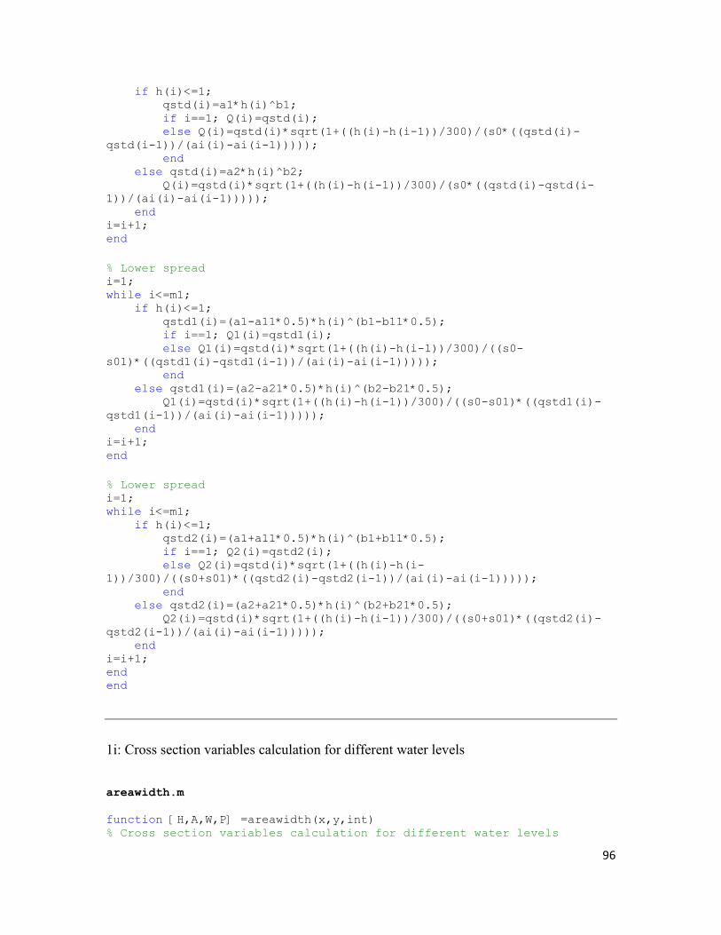
96

if h(i)<=1; qstd(i)=a1*h(i)^b1; if i==1; Q(i)=qstd(i); else Q(i)=qstd(i)*sqrt(1+((h(i)-h(i-1))/300)/(s0*((qstd(i)-qstd(i-1))/(ai(i)-ai(i-1))))); end else qstd(i)=a2*h(i)^b2; Q(i)=qstd(i)*sqrt(1+((h(i)-h(i-1))/300)/(s0*((qstd(i)-qstd(i-1))/(ai(i)-ai(i-1))))); end i=i+1; end % Lower spread i=1; while i<=m1; if h(i)<=1; qstd1(i)=(a1-a11*0.5)*h(i)^(b1-b11*0.5); if i==1; Q1(i)=qstd1(i); else Q1(i)=qstd(i)*sqrt(1+((h(i)-h(i-1))/300)/((s0-s01)*((qstd1(i)-qstd1(i-1))/(ai(i)-ai(i-1))))); end else qstd1(i)=(a2-a21*0.5)*h(i)^(b2-b21*0.5); Q1(i)=qstd(i)*sqrt(1+((h(i)-h(i-1))/300)/((s0-s01)*((qstd1(i)-qstd1(i-1))/(ai(i)-ai(i-1))))); end i=i+1; end % Lower spread i=1; while i<=m1; if h(i)<=1; qstd2(i)=(a1+a11*0.5)*h(i)^(b1+b11*0.5); if i==1; Q2(i)=qstd2(i); else Q2(i)=qstd(i)*sqrt(1+((h(i)-h(i-1))/300)/((s0+s01)*((qstd2(i)-qstd2(i-1))/(ai(i)-ai(i-1))))); end else qstd2(i)=(a2+a21*0.5)*h(i)^(b2+b21*0.5); Q2(i)=qstd(i)*sqrt(1+((h(i)-h(i-1))/300)/((s0+s01)*((qstd2(i)-qstd2(i-1))/(ai(i)-ai(i-1))))); end i=i+1; end end

1i: Cross section variables calculation for different water levels

areawidth.m

function [H,A,W,P] =areawidth(x,y,int) % Cross section variables calculation for different water levels

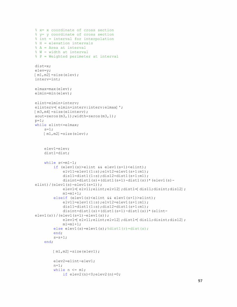
97

% x= x coordinate of cross section % y= y coordinate of cross section % int = interval for interpolation % H = elevation intervals % A = Area at interval % W = width at interval % P = Weighted perimeter at interval dist=x; elev=y; [m1,m2]=size(elev); interv=int; elmax=max(elev); elmin=min(elev); elint=elmin+interv; elinterv=[elmin+interv:interv:elmax]'; [m3,m4]=size(elinterv); aout=zeros(m3,1);width=zeros(m3,1); p=1; while elint<=elmax; s=1; [m1,m2]=size(elev); elev1=elev; dist1=dist; while s<=m1-1; if (elev1(s)>elint && elev1(s+1)<elint); elv11=elev1(1:s);elv12=elev1(s+1:m1); dis11=dist1(1:s);dis12=dist1(s+1:m1); disint=dist1(s)+(dist1(s+1)-dist1(s))*(elev1(s)-elint)/(elev1(s)-elev1(s+1)); elev1=[elv11;elint;elv12];dist1=[dis11;disint;dis12]; m1=m1+1; elseif (elev1(s)<elint && elev1(s+1)>elint); elv11=elev1(1:s);elv12=elev1(s+1:m1); dis11=dist1(1:s);dis12=dist1(s+1:m1); disint=dist1(s)+(dist1(s+1)-dist1(s))*(elint-elev1(s))/(elev1(s+1)-elev1(s)); elev1=[elv11;elint;elv12];dist1=[dis11;disint;dis12]; m1=m1+1; else elev1(s)=elev1(s);%dist1(r)=dist(s); end; s=s+1; end; [m1,m2]=size(elev1); elev2=elint-elev1; n=1; while n <= m1; if elev2(n)<0;elev2(n)=0;

98

else elev2(n)=elev2(n); end; n=n+1; end q=1;length=zeros(m1-1,1); dist2=zeros(m1-1,1); while q <= m1-1; dist2(q)=dist1(q+1)-dist1(q); q=q+1; end r=1; while r <= m1-1; if elev2(r)==0 && elev2(r+1)==0; length(r)=0; else length(r)= dist2(r); end; r=r+1; end width(p)=sum(length); m=1; trap=zeros(m1-1,1); while m <= m1-1; trap(m)=abs((dist1(m+1)-dist1(m))*(elev2(m+1)+elev2(m)))/2; m=m+1; end aout(p)=sum(trap); t=1; hypo=zeros(m1-1,1); while t<=m1-1; if elev2(t)==0 && elev2(t+1)==0; hypo(t)=0; else hypo(t)=sqrt((dist1(t+1)-dist1(t))^2+(elev2(t+1)-elev2(t))^2); end; t=t+1; end perim(p)=sum(hypo); p=p+1; elint=elint+interv; end % Outputs H=elinterv; W=width; A=aout; P=perim';

99

APPENDIX 2

Previous Reports in the Series

ISSN: (print) 1913-3200; (online) 1913-3219

1. Slobodan P. Simonovic (2001). Assessment of the Impact of Climate Variability and

Change on the Reliability, Resiliency and Vulnerability of Complex Flood Protection

Systems. Water Resources Research Report no. 038, Facility for Intelligent Decision

Support, Department of Civil and Environmental Engineering, London, Ontario,

Canada, 91 pages. ISBN: (print) 978-0-7714-2606-3; (online) 978-0-7714-2607-0.

2. Predrag Prodanovic (2001). Fuzzy Set Ranking Methods and Multiple Expert

Decision Making. Water Resources Research Report no. 039, Facility for Intelligent

Decision Support, Department of Civil and Environmental Engineering, London,

Ontario, Canada, 68 pages. ISBN: (print) 978-0-7714-2608-7; (online) 978-0-7714-

2609-4.

3. Nirupama and Slobodan P. Simonovic (2002). Role of Remote Sensing in Disaster

Management. Water Resources Research Report no. 040, Facility for Intelligent



2611-7.

4. Taslima Akter and Slobodan P. Simonovic (2002). A General Overview of

Multiobjective Multiple-Participant Decision Making for Flood Management. Water

Resources Research Report no. 041, Facility for Intelligent Decision Support,

Department of Civil and Environmental Engineering, London, Ontario, Canada, 65

pages. ISBN: (print) 978-0-7714-2612-4; (online) 978-0-7714-2613-1.

5. Nirupama and Slobodan P. Simonovic (2002). A Spatial Fuzzy Compromise

Approach for Flood Disaster Management. Water Resources Research Report no.

042, Facility for Intelligent Decision Support, Department of Civil and Environmental

Engineering, London, Ontario, Canada, 138 pages. ISBN: (print) 978-0-7714-2614-8;

(online) 978-0-7714-2615-5.

6. K. D. W. Nandalal and Slobodan P. Simonovic (2002). State-of-the-Art Report on

Systems Analysis Methods for Resolution of Conflicts in Water Resources

Management. Water Resources Research Report no. 043, Facility for Intelligent



2617-9.

7. K. D. W. Nandalal and Slobodan P. Simonovic (2003). Conflict Resolution Support

System – A Software for the Resolution of Conflicts in Water Resource Management.

100

Water Resources Research Report no. 044, Facility for Intelligent Decision Support,



8. Ibrahim El-Baroudy and Slobodan P. Simonovic (2003). New Fuzzy Performance

Indices for Reliability Analysis of Water Supply Systems. Water Resources Research

Report no. 045, Facility for Intelligent Decision Support, Department of Civil and

Environmental Engineering, London, Ontario, Canada, 90 pages. ISBN: (print) 978-

0-7714-2620-9; (online) 978-0-7714-2621-6.

9. Juraj Cunderlik (2003). Hydrologic Model Selection for the CFCAS Project:

Assessment of Water Resources Risk and Vulnerability to Changing Climatic

Conditions. Water Resources Research Report no. 046, Facility for Intelligent



2623-0.

10. Juraj Cunderlik and Slobodan P. Simonovic (2004). Selection of Calibration and

Verification Data for the HEC-HMS Hydrologic Model. Water Resources Research



0-7714-2624-7; (online) 978-0-7714-2625-4.

11. Juraj Cunderlik and Slobodan P. Simonovic (2004). Calibration, Verification and

Sensitivity Analysis of the HEC-HMS Hydrologic Model. Water Resources Research



0-7714-2626-1; (online) 978-0-7714-2627-8.

12. Predrag Prodanovic and Slobodan P. Simonovic (2004). Generation of Synthetic

Design Storms for the Upper Thames River basin. Water Resources Research Report

no. 049, Facility for Intelligent Decision Support, Department of Civil and


0-7714-2628-5; (online) 978-0-7714-2629-2.

13. Ibrahim El-Baroudy and Slobodan P. Simonovic (2005). Application of the Fuzzy

Performance Indices to the City of London Water Supply System. Water Resources

Research Report no. 050, Facility for Intelligent Decision Support, Department of

Civil and Environmental Engineering, London, Ontario, Canada, 137 pages. ISBN:

(print) 978-0-7714-2630-8; (online) 978-0-7714-2631-5.

14. Ibrahim El-Baroudy and Slobodan P. Simonovic (2006). A Decision Support System

for Integrated Risk Management. Water Resources Research Report no. 051, Facility

for Intelligent Decision Support, Department of Civil and Environmental


(online) 978-0-7714-2633-9.

101

15. Predrag Prodanovic and Slobodan P. Simonovic (2006). Inverse Flood Risk

Modelling of The Upper Thames River Basin. Water Resources Research Report no.



(online) 978-0-7714-2635-3.

16. Predrag Prodanovic and Slobodan P. Simonovic (2006). Inverse Drought Risk

Modelling of The Upper Thames River Basin. Water Resources Research Report no.



(online) 978-0-7714-2637-7.

17. Predrag Prodanovic and Slobodan P. Simonovic (2007). Dynamic Feedback Coupling

of Continuous Hydrologic and Socio-Economic Model Components of the Upper

Thames River Basin. Water Resources Research Report no. 054, Facility for

Intelligent Decision Support, Department of Civil and Environmental Engineering,

London, Ontario, Canada, 437 pages. ISBN: (print) 978-0-7714-2638-4; (online) 978-

0-7714-2639-1.

18. Subhankar Karmakar and Slobodan P. Simonovic (2007). Flood Frequency Analysis

Using Copula with Mixed Marginal Distributions. Water Resources Research Report

no. 055, Facility for Intelligent Decision Support, Department of Civil and


0-7714-2658-2; (online) 978-0-7714-2659-9.

19. Jordan Black, Subhankar Karmakar and Slobodan P. Simonovic (2007). A Web-

Based Flood Information System. Water Resources Research Report no. 056, Facility

for Intelligent Decision Support, Department of Civil and Environmental


(online) 978-0-7714-2661-2.

20. Angela Peck, Subhankar Karmakar and Slobodan P. Simonovic (2007). Physical,

Economical, Infrastructural and Social Flood Risk – Vulnerability Analyses in GIS.

Water Resources Research Report no. 057, Facility for Intelligent Decision Support,



21. Predrag Prodanovic and Slobodan P. Simonovic (2007). Development of Rainfall

Intensity Duration Frequency Curves for the City of London Under the Changing

Climate. Water Resources Research Report no. 058, Facility for Intelligent Decision

Support, Department of Civil and Environmental Engineering, London, Ontario,

Canada, 51 pages. ISBN: (print) 978-0-7714-2667-4; (online) 978-0-7714-2668-1.

22. Evan G. R. Davies and Slobodan P. Simonovic (2008). An integrated system

dynamics model for analyzing behaviour of the social-economic-climatic system:

102

Model description and model use guide. Water Resources Research Report no. 059,

Facility for Intelligent Decision Support, Department of Civil and Environmental


(online) 978-0-7714-2680-3.

23. Vasan Arunachalam (2008). Optimization Using Differential Evolution. Water

Resources Research Report no. 060, Facility for Intelligent Decision Support,



Water Resources Research Report - Faculty of … ABSTRACT River stage and discharge records are...

Documents

Transcript of Water Resources Research Report - Faculty of … ABSTRACT River stage and discharge records are...