Water-Quality and Hydrogeologic Data Used to Evaluate the ...

Water-Quality and Hydrogeologic Data Used to Evaluate the

Effects of Farming Systems on Ground-Water Quality at the

Management Systems Evaluation Area Near Princeton,

Minnesota, 1991-95

U.S. Geological Survey

Open-File Report 97-22

Prepared in cooperation with theUniversity of Minnesota Department of Soil, Water, and Climate,the U.S. Department of Agriculture,Agricultural Research Service, and theMinnesota Pollution Control Agency

Water-Quality and Hydrogeologic Data Used to Evaluate the

Effects of Farming Systems on Ground-Water Quality at the

Management Systems Evaluation Area Near Princeton,

Minnesota, 1991-95

By M.K. Landon1, G.N. Delin1, K.J. Nelson1, C.P. Regan2, J.A. Lamb3,S.J. Larson4, P.D. Capel4, J.L. Anderson3, and R.H. Dowdy5

U.S. Geological Survey

Open-File Report 97-22

Prepared in cooperation with theUniversity of Minnesota Department of Soil, Water, and Climate,the U.S. Department of Agriculture,Agricultural Research Service, and theMinnesota Pollution Control Agency

Mounds View, Minnesota

1997

1 U.S. Geological Survey, Mounds View, Minnesota2 Minnesota Pollution Control Agency, St. Paul, Minnesota3 University of Minnesota, Department of Soil, Water, and Climate, St. Paul, Minnesota4 U.S. Geological Survey, Minneapolis, Minnesota5 U.S. Department of Agriculture, Agricultural Research Service, St. Paul, Minnesota

U.S. DEPARTMENT OF THE INTERIOR

BRUCE BABBITT, Secretary

U.S. GEOLOGICAL SURVEY

Gordon P. Eaton, Director

For additional information write to: Copies of this report can be purchased from:

District Chief U.S. Geological SurveyU.S. Geological Survey Branch of Information Services2280 Woodale Drive Box 25286Mounds View, MN 55112 Denver, Colorado 80225-0286

Contents

Abstract ..................................................................................................................................................................... 1

Introduction............................................................................................................................................................... 1

Location and description of study area ..................................................................................................................... 1

Methods of investigation........................................................................................................................................... 3

Description of graphs ................................................................................................................................................ 7

Description of files on compact disk......................................................................................................................... 13

Discussion of quality assurance results..................................................................................................................... 19

Acknowledgments..................................................................................................................................................... 24

References ................................................................................................................................................................. 24

Illustrations

Figures 1-3. Maps showing:

1. Location of the Princeton, Minnesota, Management Systems Evaluation

Area in the Anoka Sand Plain. ...................................................................................................... 2

2. Study area at the Princeton, Minnesota, Management Systems Evaluation

Area................................................................................................................................................ 4

3. Layout of the research area at the Princeton, Minnesota, Management

Systems Evaluation Area. .............................................................................................................. 5

4-10. Graphs showing:

4. Background ground-water quality at multiport well B-70, 1991-95. 8

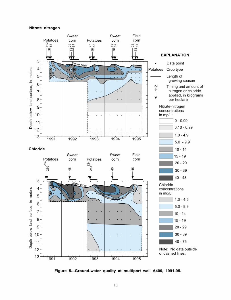
5. Ground-water quality at multiport well A400, 1991-95................................................................ 10

6. Ground-water quality at multiport well B400, 1991-95. ............................................................... 12

7. Ground-water quality at multiport well C400, 1991-95. ............................................................... 14

8. Ground-water quality at multiport well D400, 1991-95................................................................ 16

9. Ground-water quality at multiport wells E400 and R2 combined, 1991-95.................................. 18

10. Precipitation at the Princeton, Minnesota, Management Systems

Evaluation Area, 1991-95. ............................................................................................................ 20

Tables

Table 1. Laboratory detection limits and reporting limits for gas chromatography/mass spectrometry

analyses of herbicide concentrations in water from the Princeton, Minnesota,

Management Systems Evaluation Area. ............................................................................................. 7

2. Results of analyses of blanks. .............................................................................................................. 21

3. Results of analyses of replicate samples. ............................................................................................. 23

iii

Files on Compact Disk

Description File

Electronic version of report text report

Description of files on compact disk readme

Location and construction data for ground-water observation and

multiport wells and surface-water sites xyz

Geologic logs of test holes drilled during November 1992 - September 1995 well_log

Precipitation data, 1991-95 precip

Water-level data, 1990-95 watlevel

Water-level and soil temperature measurements at site MC11, 1991-95 mc11

Summary of crop activities, chemical, and irrigation applications oncropped areas, 1991 - 95 applica

Results of chemical analyses of:

Water-quality samples, April 1991 - August 1995 wat_qual

Blanks for inorganic constituents and nutrients,

April 1991 - August 1995 inofblnk

Replicate and split water samples for inorganic constituents and nutrients,

April 1991 - August 1995 inorgrep

Blanks for herbicides, April 1991 - August 1995 hrbfblnk

Laboratory blanks for herbicides, April 1991 - August 1995 hrblblnk

Replicate and split water samples for herbicides, April 1991 - August 1995 herbrep

Field spiked water samples for herbicides, April 1991 - August 1995 hrbspike

Note: All of the files listed above are in Microsoft Excel (Windows95 version 7.0, with a ‘.xls’ extension) format. The following versions of each file are also included on the compact disk in similarly named subdirectories: space-delimited (with a ‘.prn’ extension); tab-delimited (with a ‘.txt’ extension); comma-delimited (with a ‘.csv’ extension); and lotus-123 (with a ‘.wk1’ extension).

iv

Conversion Factors, Vertical Datum,and Abbreviated Water-Quality Units

Multiply By To obtain

centimeters (cm) 0.3937 inches

centimeters per day (cm/d) .3937 inches per day

centimeters per year (cm/yr) .3937 inches per year

centimeters per second (cm/s) .0328 feet per second

hectare (ha) 2.471 acres

kilograms per hectare (kg/ha) .8924 pounds per acre

kilometer (km) .6214 mile

liter (L) .2642 gallon

liter per second (L/s) 15.85 gallon per minute

meter (m) 3.281 foot

meters per year (m/yr) 3.281 feet per year

square kilometer (km2) .3861 square mile

degrees Celsius (oC) 1.8(oC)+32 degrees Fahrenheit

Sea level: In this report “sea level” refers to the National Geodetic Vertical Datum of 1929 (NGVD of 1929)--a geodetic datum derived from a general adjustment of the first-order level nets of both the United States and Canada, formerly called Sea Level Datum of 1929.

Use of brand names in this report is for identification purposes only and does not constitute endorsement by the U.S. Geological Survey.

Chemical concentrations are given in metric units. Chemical concentrations of substances in water are given in milligrams per liter (mg/L) or micrograms per liter (mg/L). Milligrams per liter is a unit expressing the concentration of chemical constituents in solution as weight (milligrams) of solute per unit volume (liter) of water. One thousand micrograms per liter is equivalent to one milligram per liter. For concentrations less than 7,000 mg/L, the numerical value is the same as for concentrations in parts per million.

v

Test Hole Numbering System

The system of numbering test holes in this report is based on the U.S. Bureau of Land Management’s system of land subdivision (township, range, and section). The system of numbering wells is shown below. In this system, the first numeral of a location number indicates the township (the N after the township number is an abbreviation for north); the second, the range (the W after the range number is an abbreviation for west); and the third, the section in which the point is located. Uppercase letters after the section number indicate the location within the section; the first letter denotes the 160-acre tract; the second, the 40-acre tract; the third, the 10-acre tract; and so forth. Letters A, B, C, and D are assigned in a counterclockwise direction, beginning in the northeast corner of each tract. The number of uppercase letters indicates accuracy of the location number. For example, the number T140NR36W14DDD indicates a test hole in the southeast 1/4 of the southeast 1/4 of the southeast 1/4 of section 14, township 140 north, range 36 west.

vi

Water-Quality and Hydrogeologic Data Used to Evaluate the Effects of

Farming Systems on Ground-Water Quality at the Management Systems

Evaluation Area near Princeton, Minnesota, 1991-95

By M.K. Landon1, G.N. Delin1, K.J. Nelson1, C.P. Regan2, J.A. Lamb3, S.J.

Larson4, P.D. Capel4, J.L. Anderson3, and R.H. Dowdy5

Abstract

The Minnesota Management Systems Evaluation Area (MSEA) project was part of a multi-scale, inter-agency initiative to evaluate the effects of agricultural management systems on water quality in the midwest corn belt. The research area was located in the Anoka Sand Plain about 5 kilometers southwest of Princeton, Minnesota. The ground-water-quality monitoring network within and immediately surrounding the research area consisted of 73 observation wells and 25 multiport wells. The primary objectives of the ground-water monitoring program at the Minnesota MSEA were to: (1) determine the effects of three farming systems on ground-water quality, and (2) understand the processes and factors affecting the loading, transport, and fate of agricultural chemicals in ground water at the site. This report presents well construction, geologic, water-level, chemical application, water-quality, and quality-assurance data used to evaluate the effects of farming systems on ground-water quality during 1991-95.

IntroductionThe Management Systems Evaluation Area (MSEA)

program is part of a multi-scale, inter-agency initiative to evaluate the effects of agricultural systems on water quality in the midwest corn belt. Five primary MSEA’s were selected to represent a variety of hydrogeologic settings and the geographic diversity of prevailing farming practices in the region (Delin and others, 1992).

The Minnesota MSEA is near the town of Princeton, Minnesota, in the Anoka Sand Plain, an area of glacial outwash covering about 4,400 km2 (fig. 1) (Anderson and others, 1991; Delin and others, 1992). Research at the Minnesota MSEA was a cooperative effort conducted primarily by the U.S. Geological Survey (USGS), the University of Minnesota Department of Soil, Water, and Climate, and the U.S. Department of Agriculture, Agricultural Research Service (USDA-ARS). The Minnesota Pollution Control Agency (MPCA) provided assistance with water-quality monitoring.

As part of the interdisciplinary research efforts at the Minnesota MSEA, ground-water quality and hydrogeology were studied. The primary objectives of the ground-water monitoring program at the Minnesota MSEA were to: (1) determine the effects of three farming systems on ground-water quality, and (2) understand the processes and factors affecting the loading, transport, and fate of agricultural chemicals in ground water at the site. This report presents well construction, geologic, water-level, chemical application, water-quality, and quality-assurance data used to evaluate the effects of farming systems on ground-water quality during 1991-95. Graphs of selected data are included as an example of the data collected.

Location and Description of Study Area

The 8.3 km2 study area is located about 5 km southwest of Princeton, Minnesota, and about 80 km northwest of Minneapolis and St. Paul (fig. 1). The

1

1 U.S. Geological Survey, Mounds View, Minnesota2 Minnesota Pollution Control Agency, St. Paul, Minnesota3 University of Minnesota, Department of Soil, Water, and Climate, St. Paul, Minnesota4 U.S. Geological Survey, Minneapolis, Minnesota5 U.S. Department of Agriculture, Agricultural Research Service, St. Paul, Minnesota

2

Figure 1.--Location of the Princeton, Minnesota, Management SystemsEvaluation Area in the Anoka Sand Plain.

EXPLANATION

Anoka Sand Plain

Minnesota

Princeton, Minnesota, ManagementSystems Evaluation Area (MSEA)

45 40'o

94o

45o

93o

St. PaulMinneapolis

PRINCETON

SANTIAGO

Base from U.S. Geological SurveyState Base Map 1:500,000, 1965

0 20 40 MILES

40 KILOMETERS200

Mi s ss p

si

i pi

River

Riv

er

Rum

Elk

River

WRIGHTMEEKER

HENNEPIN

STEARNS

RAMSEY

ANOKA

ISANTI

KANABEC PINE

MILLELACS

CHISAGO

BENTON

WASHIN

GTO

N

SHERBURNE

65-ha research area is located about in the middle of the study area (fig. 2) and adjacent to a wetland (fig. 3). Topography is undulating in the research area with a maximum change in elevation of about 2 m over a horizontal distance of about 40 m (Delin and others, 1994a). The area is drained primarily by Battle Brook, a tributary of the St. Francis River that flows into the Mississippi River. The surficial aquifer consists of an unsaturated zone of fine- to medium-grained sand and a saturated zone of medium- to coarse-grained sand to fine gravel (Delin and others, 1994a). A clayey till underlies the surficial sand and gravel aquifer (the till is less permeable than the sand). The average depth to the water table was about 3.3 m below land surface, and the average saturated thickness was about 8 m across the study area. The average horizontal hydraulic conductivity is about 0.04 cm/s. Based on this hydraulic conductivity and an average horizontal hydraulic gradient of 0.001, ground-water generally moved from west to east (fig. 3) at a an average rate of about 8 cm/d (29 m/yr). Recharge ranged from 10 to 25 cm/yr during the study. Recharge water displaced older water in the surficial aquifer downward and laterally toward the discharge area along Battle Brook. The vertical hydraulic gradient (downward) was about 0.0001. Results of recharge age determination using chlorofluorocarbons indicated an average vertical ground-water flow rate of 0.4 cm/yr in typical recharge areas (J.K. Böhlke, U.S. Geological Survey, written commun., 1996). Near Battle Brook, the hydraulic head increases with depth and ground-water flow is upward.

Methods of Investigation

Five cropped areas (fig. 3) were established in 1991 to evaluate the effects of selected farming systems on ground-water quality (Anderson and others, 1991; Delin and others, 1994a). The 1.8- to 2.7-ha cropped areas were oriented parallel to the predominant ground-water flow direction based on water-level data collected during October 1990 through March 1991. This orientation was preferred to minimize the mixing of leachates reaching the water table from the different farming systems. Subsequent monthly water-level measurements during 1991-95 indicated that the cropped areas were correctly aligned with the predominant long-term ground-water flow direction. These cropped areas were used to evaluate three farming systems (Anderson and others, 1991): (1) a corn-soybean, two-year rotation under ridge (conservation) tillage, split-nitrogen fertilizer application, nitrogen credit for legumes, and banding of herbicides, which involves application only over the crop row (area 25.4 cm wide) rather than broadcast

application over the row and furrow (91.4 cm wide) (fig. 3, cropped areas B and D); (2) a sweet corn-potato, two-year rotation with conventional full-width (disk or chisel) tillage, split-nitrogen application, banding of herbicides for sweet corn, and broadcast application of herbicides for potatoes (fig. 3, cropped areas A and C); and (3) field corn in consecutive years under conventional full-width tillage, split-nitrogen application, and broadcast application of herbicides (fig. 3, cropped area E). A buffer area around and between the cropped areas was planted with timothy and smooth brome grass in 1991 and was not treated with agricultural chemicals. The research area was planted in alfalfa during 1981-89 and in corn during 1990, prior to the implementation of the MSEA farming systems in spring 1991. Detailed records of farming practices and chemical applications prior to 1991 were not available.

A linear-move irrigation system was used as necessary to supplement rainfall. The irrigation well was completed in a confined sand and gravel aquifer that is hydraulically separated from the surficial aquifer by a confining layer of clayey till about 15 m thick (Delin and others, 1994a). The well was completed in this confined aquifer so that the hydraulic effects of pumping would be eliminated or minimized near the cropped areas. The effects of ground-water withdrawals from the irrigation well were not observed in the water levels or ground-water flow patterns of the surficial aquifer during the study.

The on-site ground-water-quality monitoring network (fig. 3) consisted of 59 observation wells and 25 multiport wells (MPORTs) (Delin and others, 1994a). In addition, 14 observation wells were located off the 65-ha field (fig. 2). Observation wells were used to measure water levels and selected wells were used for determining concentrations of agricultural chemicals. These wells were constructed of 5.1-cm inside-diameter (i.d.) galvanized-steel or polyvinyl chloride (PVC) casing with 0.6-m to 1.5-m-long stainless steel screens located at the water table or 0.15-m-long stainless steel screens installed deeper in the aquifer. The MPORT wells were located 21 m upgradient, in the middle, at the downgradient edge, and 25 m downgradient of each cropped area (fig. 3). Additional MPORTs were located in the northernmost cropped area and along a ground-water flow path into the adjacent wetland (fig. 3). Each MPORT well consisted of six, 0.6-cm i.d. stainless-steel tubes (ports 1 through 6) housed in a 5.1-cm i.d. PVC casing; each tube had a 3-cm-long screened interval (port) external to the PVC casing. In the upper 2-m of the saturated zone (ports 1 through 6), the sampling ports were installed at 0.5-m intervals with the

3

4

Princeton, Minnesota

93°38' 93°37' 93°36'

45°32'

45°31'

0 0.25 0.5 MILES

0 0.25 0.5 KILOMETERS

EXPLANATION

Base from U.S. Geological Survey 1:100,000Digital line graph map, Princeton, 1989.

Figure 2.--Study area at the Princeton, Minnesota, Management Systems Evaluation Area.

Research area, including cropped areas

Cropped area

�

�

Battle

Brook

�

��

Wooded

Area

Wooded

Area

Wooded

AreaBB-3

BB-2

BB-1

BB-4

Domestic well (Confined-drift aquifer)MN126822

(Mount Simon-Hinckley aquifer)

Domestic wellMN126569

MC20

MC23

MC12

MC14

MC31MC32

MC18

MC16

MC25

MC24

MC21

MC30

MC13

MC15

MC13

BB-3

Off-site observation well and identifier

Surface-water site and identifier

Locations of observation wells and multiport wells withinresearch area shown in figure 3

5

Base from U.S. Geological SurveyPrinceton 1:24,000 quadrangle, 1982

0

0

250 500 750 1000

100 200 300

FEET

METERS

Figure 3.--Layout of the research area at the Princeton, Minnesota,Management Systems Evaluation Area.

EXPLANATION

Cropped area and identifier

Research area, including cropped areas

Observation well and identifier, numberin parentheses indicates numberof wells at site

Multiport well and identifier

Surface-water site and identifier

Average ground-water flow direction, 1992-95

Building

The research area is located in thenortheast quarter of section 18,township T35N, range R26W

ROAD

Wooded

Area

Wooded

Area

Wetland

BattleBattle

(4)(4)

(4)(4)

BattleBattle BrookBrook

WetlandWetland

Princeton, Minn.5 Kilometers

Princeton, Minn.5 Kilometers

MC17

MC15

MC1 MC26 MC10

MC11MC19

MC38

MC36MC37

MC35

MC29MC28MC28

MC22

MC39

MC34

MC27

MC9

MC2

MC3MC3

E880

E400E400

A-30

A45

B45

C45

D45

E45

A50

B50

C50

D50

E50

A-30

A45

B45

C45

D45

E45

A50

B50

C50

D50

E50

A-70

B-30B-30

B-70

C-30C-30

C-70

D-30D-30D-70

E-30E-30

E-70E-70

D880D400D400

C880

B880

A880

A880

BB-3

E800

D800

C800C400C400

B800B400B400

A800

A400A400

R1R1

(4)(4)R1R1

R2R2

Irrigation well Linear-moveirrigation system

BB3BB3

305th Street North

13

6th

Str

ee

t

ET1 (2)MC33 (2)

ET2 (3) SP4SP3SP5

BATTLEBROOK

SP2SP1

WM1 (2)WM2 (2)

University of Minnesota climatological station

uppermost port 0.5 m above the water table to allow sample collection if the water table rose. These shallow ports were installed at all locations shown in figure 3. Delin and Landon (1996) provide a detailed description of the MPORT design and tests to evaluate use of the MPORTs to collect discrete samples at different depths. At selected locations with shallow MPORTs, MPORTs were also installed deeper in the aquifer from approximately 2 to 8 m below the water table. The deep MPORTs (ports 7 through 11) were installed at all 400-series MPORTS, B-70, D-70, R1, R2, and MC33, and were constructed similar to the shallow MPORTs except that the interval between each sampling port varied from 1 to 2 m. The number 6 and 7 sampling ports at each site were located within about 50 cm of each other vertically (file xyz on the compact disk). The observation wells and MPORT wells were installed through 10.2-cm i.d. hollow-stem augers. The augers were then removed and the natural formation was allowed to collapse around the well or MPORT. The MPORTs were used to collect water samples to evaluate ground-water quality and to measure water levels monthly to supplement observation-well data. Water levels were measured at least monthly in all MPORTs and observation wells. Delin and others (1994a) provide a more detailed description of the ground-water-quality monitoring network.

Water samples were collected from all MPORTs and selected on-site observation wells four times per year. These samples were collected during April, before agricultural chemicals were applied, in June and August during the growing season, and in October-December after crops were harvested (Delin and others, 1994a). Water samples were collected more frequently than 4 times a year from selected wells. Selected off-site observation wells were sampled at least once a year.

Sample-collection and laboratory-analysis quality-assurance/quality-control (QA/QC) protocols were followed and are described in detail by Delin and others (1994a) and Larson and others (1996). Field QA samples collected included blanks, replicates, and spikes. Specific conductance, pH, temperature, and dissolved-oxygen concentration of ground water were measured in a flow-through cell isolated from the atmosphere during pumping at each sampling site. Water samples were collected once these properties stabilized. Alkalinity titrations were performed in the field within 4 hours of sample collection. All water samples were collected and analyzed for dissolved major anions and herbicides; selected samples were analyzed for dissolved major cations and nutrients.

Analyses for concentrations of cations and anions were completed by the Geochemistry Laboratory of the Department of Geology and Geophysics at the University of Minnesota, Minneapolis, Minnesota. Cations were analyzed using inductively-coupled plasma-mass spectroscopy (ICPMS). Analytes measured by ICPMS included calcium, magnesium, sodium, potassium, silica, iron, manganese, strontium, and barium. Anions were analyzed using ion chromatography (IC). Analytes measured by IC included sulfate, fluoride, chloride, bromide, nitrate nitrogen, nitrite nitrogen, and orthophosphate. Analyses for nutrients were completed by the Research Analytical Laboratory in the Department of Soil, Water, and Climate at the University of Minnesota, St. Paul, Minnesota. Nutrient analytes included nitrite plus nitrate nitrogen, ammonium nitrogen, and total Kjeldahl nitrogen (ammonium plus organic nitrogen). Samples from selected locations during 1993-95 were analyzed for oxygen (δ18O), hydrogen (δD), and sulfur (δ34S) stable isotope compositions. These samples were analyzed using mass spectrometry at the U.S. Geological Survey Isotope Fractionation Laboratory, Reston, Virginia.

Analyses for herbicides were completed at a U.S. Geological Survey laboratory in Minneapolis, Minnesota using gas chromatography/mass spectrometry (GC/MS) (Larson and others, 1996). Herbicide analytes included atrazine (2-chloro-4-ethylamino-6-isopropylamino-s-triazine), alachlor (2-chloro-2’-6’-diethyl-N-(methoxymethyl)-acetamide), metolachlor (2-chloro-N-(2-ethyl-6-methylphenyl)-N-(2-methoxy-1-methylethyl)acetamide), and metribuzin (4-amino-6(1,1-dimethylethyl)-3-(methylthio)-1,2,4-triazin-5(4H)-one); atrazine metabolites de-ethylatrazine (DEA) (2-amino-4-chloro-6-(isopropylamino)-s-triazine) and de-isopropylatrazine (DIA) (2-amino-4-chloro-6-(ethylamino)-s-triazine); and alachlor metabolite 2,6-diethylanaline. Compound-specific reporting and detection limits were developed for each of the analytes (table 1). The detection limit was defined as the minimum concentration at which the analyte could be routinely identified by GC/MS. The reporting limit was defined as the concentration at which the analyte could be reliably and consistently quantified by GC/MS. Concentrations greater than or equal to the detection limit, but less than the reporting limit, indicated trace concentrations of the analytes. The trace concentrations indicated that the analytes were present but there was less confidence in the value than for concentrations greater than the reporting limit. In the concentration range between the detection limit and the reporting limit there was also a substantial possibility of

6

false negatives (the presence of an analyte that was not identified). Concentrations at trace levels and below the detection limit, when reported by the laboratory, were used in computing the values of the sum of atrazine plus atrazine-metabolites DEA and DIA (atrazine plus metabolites), the ratio of DEA to atrazine (DAR), the ratio of DIA to DEA (D2R), and the ratio of DIA to atrazine (DIAR).

Description of GraphsGraphs of selected ground-water-quality data

collected during 1991-95 are included as an example of the data collected during the study (figs. 4-9). The water-quality data for MPORT B-70 (fig. 4) is representative of background water-quality unaffected by the MSEA farming systems. MPORTs A400 (fig. 5), B400 (fig. 6), C400 (fig. 7), D400 (fig. 8), and E400 (fig. 9) are located in the middle of cropped areas A, B, C, D, and E, respectively, and are representative of water quality beneath each of these cropped areas. Concentrations of nitrate nitrogen, chloride, and atrazine plus metabolites, are shown for each MPORT because these constituents most clearly illustrate the linkage of chemical applications on the farming systems with chemical concentrations in the underlying ground water. Concentrations of metribuzin are shown for MPORT A400 because the effects of metribuzin applications could be seen in the ground water beneath cropped area A and for MPORT B-70 as an example of background metribuzin concentrations. Concentrations of nitrate nitrogen and atrazine are shown, in part, because drinking water standards have been developed for these

constituents by the U.S. Environmental Protection Agency (1996). The sum of concentrations of atrazine plus metabolites were selected for display instead of just atrazine because the atrazine metabolites were frequently detected in ground water at the site. DEA was the most frequently detected herbicide or herbicide metabolite in ground water at the Minnesota MSEA and was present in the greatest concentrations (Delin and others, 1995; Landon and others, 1996). DIA had a similar detection frequency and concentration range to that of atrazine. Because these metabolites were frequently detected and are derived from atrazine it is important to consider their presence in evaluating the effects of atrazine applications on ground-water quality (Liu and others, 1996).

The vertical Y axis in figures 4-9 is depth below land surface and the horizontal X axis is time. The water-table hydrograph is included as the upper boundary of the saturated zone, and reflects periods during which ground-water recharge occurred. Arrows at the top of each contoured graph show the when chemicals were applied on the overlying cropped area. Chemical concentrations are contoured in space (vertically) versus time (horizontally). Contours were drawn to reflect the downward movement of water and solutes (from the upper boundary of the water table in the diagrams) over time (to the right in the diagrams). Contour intervals were selected that best emphasize contrasts in constituent concentrations vertically in space and horizontally through time. Most of the closed contours are artifacts of the contour intervals selected. The contouring is somewhat subjective, however, due to the wide temporal (horizontal) spacing of the data points. The following assumptions were used in contouring the data shown in figures 4-9:

• The primary source of the varying chemical concentrations in ground water at each MPORT was varying chemical applications to the overlying and upgradient land areas (Delin and others, 1995).

• The primary mechanism transporting the chemicals to ground water was recharge. Recharge created a vertical component of ground-water flow that caused the water and chemicals to move by piston displacement through the unsaturated and saturated zones. Ground-water ages inferred from chlorofluorocarbon concentrations indicate that the magnitude of this vertical ground-water flow below the water table was about 0.4 m/yr.

• Chemical loading upgradient of each MPORT was areally uniform following a particular recharge event due to areally uniform land use.

Table 1.—Laboratory detection limits and reporting limits for gas chromatography/mass spectrometry analyses of herbicide concentrations in water from the Princeton, Minnesota, Management Systems

Evaluation Area (Larson and others, 1996).[µg/L, micrograms per liter]

Herbicide or herbicide metabolites

Laboratory detection limit

(µg/L)

Laboratory reporting limit

(µg/L)

Atrazine 0.01 0.04

De-ethylatrazine .03 .06

De-isopropylatrazine .06 .08

Alachlor .01 .04

2,6-diethylanaline .01 .04

Metolachlor .01 .04

Metribuzin .03 .06

7

8

Nitrate-nitrogenconcentrationsin mg/L:

1.0 - 4.9

5.0 - 9.9

10 - 14

15 - 19

0 - 0.99

0.10 - 0.99

1.0 - 4.9

5.0 - 9.9

10 - 14

15 - 18

Chlorideconcentrationsin mg/L:

Note: No data outsideof dashed lines.

De

pth

be

low

lan

dsu

rfa

ce,

inm

ete

rs

3

4

5

6

7

8

9

10

11

12

131991 1992 1993 1994 1995

EXPLANATION

Chloride

Nitrate nitrogen

Figure 4.--Background ground-water quality at multiport well B-70, 1991-95.

Data point

Grass

Grass GrassGrass Grass Grass

Vegetation

Water table

De

pth

be

low

lan

dsu

rfa

ce,

inm

ete

rs

3

4

5

6

7

8

9

10

11

12

131991 1992 1993 1994 1995


Water table

20 - 25

9

0 - 0.02

0.03 - 0.11

Metribuzin concentrations

in g/L:�

De

pth

be

low

lan

dsu

rfa

ce,

inm

ete

rs

3

4

5

6

7

8

9

10

11

12

131991 1992 1993 1994 1995

Water table


De

pth

be

low

lan

dsu

rfa

ce,

inm

ete

rs

3

4

5

6

7

8

9

10

11

12

131991 1992 1993 1994 1995

Water table

Metribuzin

Atrazine plus atrazine metabolites de-ethylatrazine and de-isopropylatrazine

Data point

Grass Vegetation


Figure 4.--continued.

Atrazine plus metabolite

concentrations in g/L:�

0 - 0.04

0.05 - 0.19

0.20 - 0.49

0.50 - 0.99

1.00 - 1.38

EXPLANATION


10

EXPLANATION


1.0 - 4.9

0.10 - 0.99

5.0 - 9.9

10 - 14

15 - 19

0 - 0.09

1.0 - 4.9

5.0 - 9.9

10 - 14

15 - 19


20 - 29

30 - 39

40 - 48

20 - 29

30 - 39

40 - 75

De

pth

be

low

lan

dsu

rfa

ce,

inm

ete

rs

3

4

5

6

7

8

9

10

11

12

131991 1992 1993 1994 1995

Water table

Potatoes PotatoesSweetcorn

Sweetcorn

Fieldcorn

112

56

56

11

2

22

67

78

76

56

56

22

78

62

22

78

67

Figure 5.--Ground-water quality at multiport well A400, 1991-95.

Data point

Timing and amount ofnitrogen or chlorideapplied, in kilogramsper hectare

Length ofgrowing season

Potatoes Crop type

De

pth

be

low

lan

dsu

rfa

ce,

inm

ete

rs

3

4

5

6

7

8

9

10

11

12

131991 1992 1993 1994 1995

Water table


Sweetcorn

Fieldcorn

22

4

22

4

28

0

25

3

45

45

45

Chloride

Nitrate nitrogen


11

EXPLANATION

De

pth

be

low

lan

dsu

rfa

ce,

inm

ete

rs

3

4

5

6

7

8

9

10

11

12

131991 1992 1993 1994 1995

Water table


Sweetcorn

Fieldcorn

0.4

0

0.4

0

0.4

7

0.4

7


Data point

Timing and amount ofatrazine or metribuzinapplied, in kilograms

per hectare


Potatoes Crop type

De

pth

be

low

lan

dsu

rfa

ce,

inm

ete

rs

3

4

5

6

7

8

9

10

11

12

131991 1992 1993 1994 1995

Water table


Sweetcorn

Fieldcorn

0.5

6

0.4

1



0 - 0.04

0 - 0.02

0.05 - 0.19

0.03 - 0.19

0.20 - 0.49

0.20 - 0.49

0.50 - 0.92

0.50 - 0.70

Metribuzin concentrations

in g/L:�

Metribuzin



12

EXPLANATION

De

pth

be

low

lan

dsu

rfa

ce,

inm

ete

rsD

ep

thb

elo

wla

nd

surf

ace

,in

me

ters

3

3

4

4

5

5

6

6

7

7

8

8

9

9

10

10

11

11

12

12

13

13

1991

1991

1992

1992

1993

1993

1994

1994

1995

1995

Water table

Water table

Soybeans

Soybeans

Soybeans

Soybeans

Soybeans

Soybeans

Fieldcorn

Fieldcorn

Fieldcorn

Fieldcorn

112

22

22

56

78

45

22

62

28

78

20

45

Figure 6.--Ground-water quality at multiport well B400, 1991-95.

Data point



Soybeans Crop type

Chloride

Nitrate nitrogen


0 - 0.09

1.0 - 4.9

0.10 - 0.99

5.0 - 9.9

10 - 14

15 - 18

1.0 - 4.9

5.0 - 9.9

10 - 14

15 - 19

20 - 29

30 - 39

40 - 42



EXPLANATION

De

pth

be

low

lan

dsu

rfa

ce,

inm

ete

rs

3

4

5

6

7

8

9

10

11

12

131991 1992 1993 1994 1995

Water table

Soybeans Soybeans SoybeansFieldcorn

Fieldcorn

0.5

6

0.5

6

0.4

7


Data point

Timing and amount ofatrazine applied, inkilograms per hectare


Soybeans Crop type



concentrations in g/L:�0 - 0.04

0.05 - 0.19

0.20 - 0.49

0.50 - 0.71


• Chemical concentrations measured at each sampling port were related to chemical concentrations at shallower and deeper sampling ports. This assumption is plausible given the relatively low vertical rates of ground-water flow compared to the average horizontal rate of about 29 m/yr. It should be kept in mind, however, that water from each successively deeper sampling port had a recharge source area that was successively further upgradient from the MPORT.

• Chemical concentrations for each sampling period were related to chemical concentrations for earlier and later sampling periods. The average vertical and horizontal ground-water flow rates were slow enough that the chemicals in the upper part of the saturated zone were not flushed out of the profile before the next sampling.

Monthly and daily precipitation during 1991-95 are shown in figure 10. Most of the data for April through October of each year were measured at the University of Minnesota climatological station at the MSEA (fig. 3).

Where necessary, however, the University of Minnesota measurements were supplemented by precipitation measurements at sites R1 and R2 (fig. 3). Precipitation data for November through March of each year were measured by the National Weather Service (National Oceanic and Atmospheric Administration, electronic commun., 1996) at Santiago, Minnesota, about 20 km west of the research site (fig. 1).

Description of Files on Compact DiskThe data included on the compact disk are duplicated

in several formats with an identical filename prefix. Files of a particular format are in separate subdirectories. File formats include: Microsoft Excel workbook or spreadsheet (Windows 95, Version 7.0, file extension ‘.xls’), space-delimited text (file extension ‘.prn’), tab-delimited text (file extension ‘.txt’), comma-delimited text (file extension ‘.csv’), and Lotus spreadsheet (file extension ‘.wk1’). At least one of the text versions of the files should import into any software package. Following is a brief description of the types of information included in each data file.

13

14

EXPLANATION

1.0 - 4.9

5.0 - 9.9

10 - 14

15 - 19

20 - 29

30 - 39

40 - 53


De

pth

be

low

lan

dsu

rfa

ce,

inm

ete

rsD

ep

thb

elo

wla

nd

surf

ace

,in

me

ters

3

3

4

4

5

5

6

6

7

7

8

8

9

9

10

10

11

11

12

12

13

13

1991

1991

1992

1992

1993

1993

1994

1994

1995

1995

Water table

Water table

Potatoes

Potatoes

Potatoes

Potatoes

Sweetcorn

Sweetcorn

Sweetcorn

Sweetcorn

Wheat

Wheat

22

112

78

78

22

2

78

45

22

67

67

52

6

62

15

67

34

34

46

67

22

4

56

22

Figure 7.--Ground-water quality at multiport well C400, 1991-95.

Data point



Sweetcorn

Crop type

Chloride

Nitrate nitrogen


1.0 - 4.9

0.10 - 0.99

5.0 - 9.9

10 - 14

15 - 19

20 - 29

30 - 32


EXPLANATION

De

pth

be

low

lan

dsu

rfa

ce,

inm

ete

rs

3

4

5

6

7

8

9

10

11

12

131991 1992 1993 1994 1995

Water table


Sweetcorn Wheat

0.4

7

0.4

7

0.4

7


Data point



Sweetcorn

Crop type




0 - 0.04

0.05 - 0.19

0.20 - 0.49

0.50 - 0.65


The text of this report is included in Microsoft Word format (Windows 95 Version 7.0, file extension ‘.doc’) and text format (file extension ‘.txt’). The ‘readme’ file contains a brief description of the contents of the compact disk.

Location and well-construction information for each of the monitoring wells and MPORTs installed during 1990-95 are included in the ‘xyz’ file. Included is the depth of the top and bottom of the well screen below the measuring point and below land surface, elevation of the measuring point, elevation of the top and bottom of the well screen, stickup height, and date of installation. The horizontal location of the each site is given in meters from the local coordinate system origin, which is well MC1, in the southwest corner of the research area.

Geologic logs for observation wells and MPORTs installed during November 1992 - September 1995 are given in the ‘well_log’ file. Geologic logs for wells installed during 1990-92 were previously given in Delin and others (1994b).

Included in the ‘precip’ file is the hourly precipitation (when available), total daily, monthly, and annual precipitation, during 1991-95. Also included is the source of the data, either the University of Minnesota climatological station (fig. 3), precipitation gages at sites R1 or R2 (fig. 3), or the National Weather Service station at Santiago, Minnesota (fig. 1).

Data for water levels measured with an electronic or steel tape during 1990-95 are included in the ‘watlevel’ file. Water levels were measured approximately monthly in all wells. Water levels were measured more frequently in selected wells to fulfill other research objectives.

Water-level and soil-temperature data measured hourly to daily and recorded on a datalogger at observation well MC11 during 1991-95 are included in the ‘mc11’ file. Water levels were measured using a shaft encoder connected to the datalogger. Periodic water-level measurements with a steel tape were made to check the water levels measured with the shaft encoder and are also included in the file. Soil

15

16

1.0 - 4.9

5.0 - 9.9

10 - 14

15 - 19

20 - 30


De

pth

be

low

lan

dsu

rfa

ce,

inm

ete

rsD

ep

thb

elo

wla

nd

surf

ace

,in

me

ters

3

3

4

4

5

5

6

6

7

7

8

8

9

9

10

10

11

11

12

12

13

13

1991

1991

1992

1992

1993

1993

1994

1994

1995

1995

Water table

Water table

Soybeans

Soybeans

Soybeans

Soybeans

Fieldcorn

Fieldcorn

Fieldcorn

Fieldcorn

Fieldcorn

Fieldcorn

22

78

56

45

22

67

20

22

20

56

45

67

34

56

112

22

Figure 8.--Ground-water quality at multiport well D400, 1991-95.

Data point



Fieldcorn

Crop type

Chloride

Nitrate nitrogen

9

EXPLANATION


0 - 0.09

1.0 - 4.9

0.10 - 0.99

5.0 - 9.9

10 - 14

15 - 19

20 - 24


epth

belo

land

sur

ace

inm

ete

rs

8

ater table

oybeans oybeansFieldcorn

Fieldcorn

Fieldcorn

. ..

.


ata point

Timing and amountatrazine applied inilograms per hectare

Length ogro ing season

Fieldcorn

rop type

Atrazine plus atrazine metabolit es de-ethylatrazine and de-isopropylatrazine

EXPLANATION

Atrazine plus metabolites

concentrations in g L�- .

. - .

. - .

. - .

Note No data outsideo dashed lines.

temperatures at 5 depths were measured using buried thermocouples. A reference thermistor was also installed on the datalogger for compensating the temperature measurements made by the thermocouples. Data were recorded on dataloggers at several other sites in the research area. These results are presented in a separate data report (Delin and others, 1997).

The amounts and times of fertilizer, herbicide, and irrigation water application to the five cropped areas are included in the ‘applica’ file. Also included are the approximate timing of crop planting and harvesting on each cropped area during 1991-95. Chemicals applied to the cropped areas include nitrogen (from ammonia fertilizer [urea], diammonium phosphate, ammonium sulfate, and ammonium nitrate), potassium (from potassium chloride, potassium magnesium sulfate, and potassium bromide), chloride (from potassium chloride), magnesium (from potassium magnesium sulfate), phosphorus (from diammonium phosphate), sulfur (from zinc sulfate, potassium magnesium sulfate, and ammonium sulfate), zinc (from zinc sulfate), atrazine, alachlor, metribuzin, and metolachlor.

Results of water-quality analyses of ground-water and surface-water samples collected during April 1991 through August 1995 are included in the ‘wat_qual’ file. Sampling data from April 1991 were previously published in Delin and others (1994b). Interpretations of selected ground-water quality results were discussed in Delin and others (1994a, 1995) and Landon and others (1996). Water-quality data collected as part of other research are presented in a separate data report (Delin and others, 1997).

Results of the analyses of QA samples collected during April 1991 through August 1995 are included in several files. The QA samples included blanks, replicates, splits, and spikes. Descriptions of each of these sample types and collection procedures are given in Delin and others (1994a) and Larson and others (1996). Results of analyses of blanks for inorganic constituents and nutrients are included in the ‘inofblnk’ file. Results of analyses of replicate and split water samples for inorganic constituents and nutrients are included in the ‘inorgrep’ file. Results of analyses of blanks for herbicides are included in the ‘hrbfblnk’ file.

17

18


0 - 0.09

1.0 - 4.9

0.10 - 0.99

5.0 - 9.9

10 - 14

15 - 19

20 - 26

EXPLANATION

De

pth

be

low

lan

dsu

rfa

ce,

inm

ete

rsD

ep

thb

elo

wla

nd

surf

ace

,in

me

ters

3

3

4

4

5

5

6

6

7

7

8

8

9

9

10

10

11

11

12

12

13

13

1991

1991

1992

1992

1993

1993

1994

1994

1995

1995

Water table

Water table

Fieldcorn

Fieldcorn

Fieldcorn

Fieldcorn

Fieldcorn

Fieldcorn

Fieldcorn

Fieldcorn

Fieldcorn

Fieldcorn

78

78

78

45

45

45

45

22

22

22

22

22

67

67

67

62

78

78

58

112

22

Figure 9.--Ground-water quality at multiport wells E400 and R2 combined, 1991-95.

Data point



Fieldcorn

Crop type

Chloride

Nitrate nitrogen

1.0 - 4.9

5.0 - 9.9

10 - 14

15 - 19

20 - 29

30 - 39

40 - 48



EXPLANATION

De

pth

be

low

lan

dsu

rfa

ce,

inm

ete

rs

3

4

5

6

7

8

9

10

11

12

131991 1992 1993 1994 1995

Water table

Fieldcorn

Fieldcorn

Fieldcorn

Fieldcorn

Fieldcorn

1.6

8

1.6

8

1.6

8

1.6

8

1.6

8

1.6

8Figure 9.--continued.

Data point



Fieldcorn

Crop type



concentrations in g/L:�0 - 0.04

0.05 - 0.19

0.20 - 0.49

0.50 - 0.99

1.00 - 1.99

2.00 - 2.99

3.00 - 4.30


Results of analyses of laboratory blanks for herbicides are included in the ‘hrblblnk’ file. Results of analyses of replicate and split water samples for herbicides are included in the ‘herbrep’ file. Results of analyses of water samples spiked with herbicides in the field are included in the ‘hrbspike’ file.

Discussion of Quality Assurance Results

The QA data indicate that the water-quality data collected are suitable for fulfilling the objectives of the study. However, some of the blank data has implications for the interpretation of the concentrations of some constituents at low concentrations.

Trace levels of most analytes were found in some blanks (table 2). Blanks were samples of “analyte-free” water that were processed through the sampling equipment, after using the field equipment cleaning procedures (Delin and others, 1994a). About 3 percent of the samples analyzed were blanks. Possible sources of contamination detected in blanks include the: 1) sampling equipment, 2) “analyte-free” water used for

the blank, 3) sample bottles in which the blank was collected, 4) sample preservation solutions for the cation samples, which were acidified with 6.0-Normal hydrochloric acid, or 5) laboratory analysis. It was usually not possible to determine the source of the contamination in the blanks, which could have occurred from any of these sources. Therefore, the blank results indicate the cumulative contamination that occurred as a result of the sample collection and analysis.

Blanks were collected in the field under conditions that resulted in a greater risk of contamination than for environmental water samples, primarily for two reasons. First, the volume of water flushed through the sampling equipment prior to collection of the blank, (0.5-1.0 L) was much less than for environmental samples (7-10 L). The reduced pre-sampling rinse reduces the chance of flushing any contaminants present in the sampling equipment out prior to sample collection. Second, the blank water was susceptible to contamination during collection from sources other than the sampling equipment. Sources of contamination include dust and intermediate containers used to hold blank water. There

19

21

1The upper limit of the range shown represents the greatest reliable concentration, which was the greatest concentration found in more than one sample or that was very close in magnitude to the next lowest concentration. In cases where the maximum was anomalously large, the actual maximum was excluded because contamination of the blanks likely was not related to the sampling process.

2Concentrations less than the ERL could be partially or wholly an artifact of contamination from the sampling process. The ERL rep-resents the maximum possible contamination from the sampling process. Typical contamination from the sampling process was less.

3Atrazine concentrations ≤0.02 may partially or wholly reflect contamination from sampling equipment in some samples. This concen-tration is < the laboratory reporting limit of 0.04 µg/L.

4Detections in blanks for DEA and metribuzin were so infrequent that they were anomalous and do not indicate persistent contamination problems for these constituents.

5Alachlor concentrations ≤ 0.07 may partially or wholly reflect contamination from sampling equipment in some samples. This con-centration is greater than the laboratory reporting limit of 0.04 µg/L.

Table 2.—Results of analyses of blanks.[mg/L, milligrams per liter; µg/L, micrograms per liter; %, percent; DL, detection limit; <, less than; na, not applicable; =, equals; ERL, effective reporting

limit; ≤, less than or equal to; concentrations of constituents are expressed as mass of the element or constituent listed except where otherwise noted, for example, nitrate (as nitrogen)]

ConstituentsNumber of blanks

% of blanks

above DLLaboratory

DLRange of blank concentrations1

% of field samples in range of blank

detections Action taken/notes

Inorganics and nutrients (concentrations in mg/L)

Silica (as silicon) 25 84 0.01 0.01-0.32 lowest 0.1 % set ERL to 0.3 mg/L2

Manganese 25 84 .0001 .0001-.0028 40% (7% also below DL) set ERL to .003 mg/L2

Iron 25 64 .0001 .0001-.0288 34% (27% also below DL) set ERL to .03 mg/L2

Strontium 25 92 .0001 .0001-.0030 lowest .1 % set ERL to .003 mg/L2

Barium 25 72 .0001 .0001-.0036 0% none

Magnesium 25 84 .01 .01-.27 lowest .1 % set ERL to .3 mg/L2

Calcium 25 96 .01 .01-.99 lowest .1 % set ERL to 1.0 mg/L2

Sodium 25 88 .01 .01-.46 lowest .2 % set ERL to .5 mg/L2

Potassium 25 80 .01 .01-.29 lowest 3 % set ERL to .3 mg/L2

Chloride 55 78 .01 .01-.59 lowest 3 % set ERL to .6 mg/L2

Bromide 52 0 .02 <.02 na none

Nitrite (as nitrogen) 52 0 .01 <.01 na none

Nitrate (as nitrogen) 61 20 .01 .01-.20 3% (5% also below DL) set ERL to .2 mg/L2

Sulfate 52 33 .03 .03-.35 lowest .05% none

Orthophosphate(as phosphorus)

52 0 .03 <.03 na none

Fluoride 52 0 .01 <.01 na none

Ammonia (as nitrogen) 18 0 .02 <.02 na none

Total Kjeldahl nitrogen 10 10 .20 .20-.25 13% (71% also below DL) set ERL to .25 mg/L2

Organics and herbicides (concentrations in µg/L except for TOC, which is in mg/L)

Total organic carbon (TOC)

4 na none .60-1.35 73% set ERL to 1.35 mg/L2

Atrazine 58 28 .01 .01-.02 43% (38% also below DL) none, ERL = .04 µg/L3

De-ethylatrazine (DEA) 58 3 .03 .03-.04 23% (10% also below DL) none, ERL = .06 µg/L 4

De-isopropylatrazine 58 0 .06 <.06 na none, ERL = .08 µg/L

Alachlor 58 12 .01 .01-.07 12% (87% also below DL) set ERL to .07 µg/L5

2,6-diethylanaline 58 0 .01 <.01 na none, ERL = .04 µg/L

Metolachlor 58 0 .01 <.01 na none, ERL = .04 µg/L

Metribuzin 58 2 .03 .03-.09 8% (90% also below DL) none, ERL = .06 µg/L4

was a much greater chance for contamination of the blank water from dust than for the environmental samples, which were only exposed to the atmosphere for the distance from the end of the sampling tube to the collection bottle. Because the concentrations measured in the blanks were small, a small amount of contamination during any of several steps in the blank collection process was sufficient to result in contamination of the blank sample. The overall effect of the greater risk of contamination for blanks is that the concentrations measured in the blanks probably overestimate the concentrations imparted to the environmental water samples in the sampling and analysis process. This caveat does not render the blank data useless, but indicates that it should be used cautiously.

Rather than censoring actual data that may or may not have been affected by contamination, it was decided to establish effective reporting limits as criteria for indicating the amount of uncertainty associated with the reported concentration. The concentrations reported by the analytical laboratories are presented in the files on the compact disk. These values were not altered even when they were below the effective reporting limit. The general approach taken was to select the highest reliable concentration in blanks and to define that concentration as the effective reporting limit for that constituent (table 2). The highest reliable concentration was the highest concentration that was found in more than one blank sample or that was very close in magnitude to the next lowest concentration. The highest reliable concentration in blanks did not always correspond to the maximum concentration. If the maximum concentration substantially exceeded the next lowest concentration, the maximum was considered unrepresentative of concentrations imparted to the blank water by the sampling process and was disregarded. This is reasonable given the substantial risk of contaminating the blank during collection from sources unrelated to the sampling process.

The effective reporting limit (ERL) has the following consequences: 1) Concentrations less than the ERL may partially or wholly reflect contamination and not represent environmental concentrations. Thus, there is more uncertainty associated with concentrations below the ERL. 2) The ERL represents only the maximum possible level of contamination; typical inputs from the sampling process would usually be less. 3) Concentrations in environmental samples greater than the ERL represent maximum concentrations because some fraction of the concentration could be from the sampling process. However, concentrations of most

constituents in environmental samples were much greater than in blanks (table 2) and any contaminants from the sampling process would be imperceptible.

There were no detections of bromide, nitrite, orthophosphate, fluoride, ammonia, de-isopropylatrazine, 2,6-diethylanaline, and metolachlor in any of the blanks. For silica, strontium, barium, magnesium, calcium, sodium, and sulfate, less than 0.2 percent of the environmental samples were in the range of the concentrations detected in the blanks (table 2). For potassium, chloride, and nitrate, less than 3 percent of the environmental samples overlapped with the concentrations in blanks. Thus, detections of these constituents in blanks created uncertainty in only a few of the samples with the very lowest concentrations and had no effect on most of the data. Similarly, metribuzin was detected in one and de-ethylatrazine in two of the blank samples; these low detection frequencies (2 to 3 percent) were anomalous and do not indicate persistent contamination problems.

Manganese, iron, and total Kjeldahl nitrogen were detected below the ERL in 40, 34, and 13 percent, respectively, of the environmental samples (table 2). These percentages do not include the substantial number of field samples that had concentrations below the detection limit for these constituents; samples with concentrations below the detection limit were clearly not affected by contamination from the sampling process. Total organic carbon was detected below the ERL in 73 percent of the environmental samples. Thus, only 27 percent of environmental samples were above the ERL of 1.35 mg/L (table 2).

Atrazine was detected in 28 percent of the blanks at concentrations of 0.01 to 0.02 (mostly 0.01) µg/L (table 2; file ‘hrbfblnk’ on compact disk). Atrazine was also detected in 12 percent of laboratory blanks at concentrations of 0.01 to 0.02 µg/L (file ‘hrblblnk’ on compact disk). Detections in the laboratory blanks indicate trace-level contamination during laboratory analysis. Some of the detections in blanks may be artifacts of the laboratory contamination. Atrazine concentrations in environmental samples were below the detection limit of 0.01 µg/L in 38 percent, 0.01 to 0.02 µg/L in 43 percent, and greater than concentrations in blanks in 19 percent of the samples. These results indicate that sample contamination may be the cause of some of the detections of atrazine at concentrations of 0.01 to 0.02 µg/L in environmental samples. However, because the percentage of environmental samples having these concentrations are greater than the percentages in field or laboratory blanks, it is likely that some of the detections in the field at these

22

Table 3.—Results of analyses of replicate samples.[%, percent; CV, coefficient of variation (expresses the standard deviation as a percent of the mean); <, less than]

ConstituentsNumber of

sets of replicates CV criteria

Percentage of replicate sets with CV < CV criteria

Inorganics and nutrients

Silica (as silicon) 26 5% 96%

Manganese 26 5% 54%

Iron 26 10% 62%

Strontium 26 5% 100%

Barium 26 5% 73%

Magnesium 26 5% 96%

Calcium 26 5% 96%

Sodium 26 5% 85%

Potassium 26 5% 73%

Chloride 52 5% 83%

Bromide 48 5% 90%

Nitrite (as nitrogen) 49 5% 96%

Nitrate (as nitrogen) 64 5% 89%

Sulfate 49 5% 96%

Orthophosphate (as phosphorus) 49 5% 100%

Fluoride 45 5% 89%

Ammonia (as nitrogen) 19 5% 89%

Total Kjeldahl nitrogen 12 10% 58%

Organics and herbicides

Total organic carbon 6 15% 67%

Atrazine 89 25% 52%

De-ethylatrazine 89 25% 58%

De-isopropylatrazine 89 25% 78%

Alachlor 89 25% 89%

2,6-diethylanaline 86 25% 100%

Metolachlor 89 25% 97%

Metribuzin 89 25% 91%

concentrations reflect actual environmental concentrations. Because the laboratory reporting limit of 0.04 µg/L was greater than the largest reliable blank detection of 0.02 µg/L, the reporting limit for atrazine was not modified.

Alachlor was detected in 12 percent (6 samples) of the blanks analyzed at concentrations of 0.01, 0.01, 0.03, 0.03, 0.05, and 0.07 µg/L. Alachlor was also detected in 5 percent of laboratory blanks at a concentration of 0.01 µg/L. Some of the detections in blanks may be artifacts of laboratory contamination. Alachlor concentrations in environmental samples were below the detection limit in 87 percent, in the same range as blanks in 12 percent, and greater than

concentrations in blanks in 1 percent. Because the percentage of environmental samples having concentrations of 0.01 to 0.07 µg/L is the same as the percentage in blanks, it is possible that most or all the detections in environmental samples at these concentrations are an artifact of contamination from the sampling and laboratory analysis process. Therefore, the effective reporting limit for alachlor was increased to 0.07 µg/L.

Results of analyses of replicate samples indicated that measured concentrations were satisfactorily reproducible (table 3). Replicates consisted of triplicate samples collected from the same sampling location at

23

the same time. Water was collected in a large sampling container and then subsampled from this larger container into individual replicate samples (Delin and others, 1994a). Replicate samples accounted for 8 to 14 percent of the samples analyzed. Results indicated that the coefficient of variation in most replicate samples was less than 25 percent for herbicides, less than 15 percent for total organic carbon, less than 10 percent for iron and Kjeldahl nitrogen, and less than 5 percent for all other inorganic and nutrient constituents. The lesser precision for herbicide analyses reflects the higher degree of analytical uncertainty inherent in quantifying trace organics at the very low concentrations measured (usually less than 0.1 µg/L).

Results of field spikes for herbicides indicated that average recoveries for all herbicides, other than 2,6-diethylanaline, were 83 to 104 percent (file ‘hrbspike’ on compact disk). Field spikes at concentrations of both 0.05 and 0.10 µg/L indicated similar high recoveries, indicating good measurement accuracy. Field spikes comprised about 3 percent of the herbicide analyses (Delin and others, 1994a). The average spike recovery for 2,6-diethylanaline was 21 percent. The low recovery for this alachlor metabolite indicates either that the compound underwent degradation after the sample was collected (loss) or that the compound was not efficiently isolated by the solid-phase extraction column in the volume of water used in the analysis. This result indicates that reported concentrations for 2,6-diethylanaline should be considered minima and that false negatives are possible.

The ion balance shows the degree to which the charges of cations measured in a sample are balanced by the charges of anions. Since water is charge-neutral, an analysis of cations and anions dissolved in water should ideally produce a charge balance of zero. For 976 water samples in which both cations and anions were measured, the charge balance was within 5 percent, with 95 percent of the samples having a balance less than 1.8 percent, and a median of 0.7 percent.

AcknowledgmentsThe authors are grateful to the many employees of the

Minnesota Pollution Control Agency, Department of Soil, Water, and Climate at the University of Minnesota, U.S. Department of Agriculture, Agricultural Research Service, and the U.S. Geological Survey who contributed to the data collection and analysis. The authors are also grateful to Lifeng Guo and Dr. E.C. Alexander at the Department of Geology and Geophysics at the University of Minnesota for assistance with data collection. The authors are also

grateful to Berlinson and Associates, the land owners, for leasing the land to the University of Minnesota.

ReferencesAlexander, R.B., and Smith, R.A., 1990, County-level

estimates of nitrogen and phosphorus fertilizer use in the United States, 1945 to 1985: U.S. Geological Survey Open-File Report 90-130, 12 p.

Anderson, J.L., Dowdy, R.H., and Delin, G.N., 1991, Ground water impacts from irrigated ridge-tillage, in Ritter, W.F., ed., Proceedings of the American Society of Civil Engineers, 1991 National Conference on Irrigation and Drainage Engineering, Honolulu, Hawaii, July 23-26, 1991, p. 604-610.

Delin, G.N. and Landon, M.K., 1996, Multiport well design for sampling of ground water at closely-spaced vertical intervals: Ground Water, vol. 34, no. 6, p. 1098-1104.

Delin, G.N., Landon, M.K., Anderson, J.L., and Dowdy, R.H., 1992, Hydrologic research at the Princeton, Minnesota, Management Systems Evaluation Area: U.S. Geological Survey Open-File Report 92-107, 2 p.

Delin, G.N., Landon, M.K., Lamb, J.A., and Anderson, J.L., 1994a, Characterization of the hydrogeology and water quality at the Management Systems Evaluation Area near Princeton, Minnesota, 1991-92: U.S. Geological Survey Water-Resources Investigations Report 94-4149, 54 p.

_____1994b, Hydrogeologic and water-quality data used to characterize the Management Systems Evaluation Area (MSEA) near Princeton, Minnesota: U.S. Geological Survey Open-File Report 94-337, 45 p.

Delin, G.N., Landon, M.K., Lamb, J.A., and Dowdy, R.H., 1995, Effects of 1992 farming systems on ground-water quality at the Management Systems Evaluation Area near Princeton, Minnesota: U.S. Geological Survey Water-Resources Investigations Report 95-4104, 23 p.

Delin, G.N., Landon, M.K., Nelson, K.J., Wanty, R.B., and Healy, R.W., 1997, Hydrogeologic and water-quality data used to evaluate the effects of focused recharge on ground-water quality near Princeton,

24

Minnesota: U.S. Geological Survey Open-File Report 97-21, 30 p.

Landon, M.K., Delin, G.N., Lamb, J.A., Dowdy, R.H., and Anderson, J.L., 1996, Effects of farming systems on ground-water quality at the Princeton, Minnesota, Management Systems Evaluation Area, 1991, in Morganwalp, D.W., and Aronson, D.A., eds., U.S. Geological Survey Toxic Substances Hydrology Program--Proceedings of the technical meeting, Colorado Springs, Colorado, September 20-24, 1993: U.S. Geological Survey Water-Resources Investigations Report 94-4015, p. 543-554.

Larson, S.J., Capel, P.D., VanderLoop, A.G., 1996, Laboratory and quality assurance protocols for the analysis of herbicides in ground water from the Management Systems Evaluation Area, Princeton, Minnesota: U.S Geological Survey Water-Resources Investigations Report 95-4178, 18 p.

Liu, S., Yen, S.T., and Kolpin, D.W., 1996, Pesticides in ground water-- Do atrazine metabolites matter?: Water Resources Bulletin, vol. 32, no. 4, p. 845-853.

U.S. Environmental Protection Agency, 1996, Drinking water regulations and health advisories: U.S. Environmental Protection Agency, February 1996, 11 p.

25

Water-Quality and Hydrogeologic Data Used to Evaluate the ...

Documents

Transcript of Water-Quality and Hydrogeologic Data Used to Evaluate the ...