TECHNICAL GUIDANCE MANUAL FOR HYDROGEOLOGIC INVESTIGATIONS ...
497
Transcript of TECHNICAL GUIDANCE MANUAL FOR HYDROGEOLOGIC INVESTIGATIONS ...


TECHNICAL GUIDANCE MANUAL FOR HYDROGEOLOGICINVESTIGATIONS AND GROUND WATER MONITORING
Division of Drinking and Ground WatersOhio Environmental Protection Agency
122 South Front StreetColumbus, Ohio 43126-1049
February 1995

-iii-
NOTICE
A draft version of this document was issued for public comment on July 22, 1993. Thecomment period ended on December 10, 1993. Comments received were consideredin the development of this final document.
Figures that were duplicated from non-government sources were used with permissiongranted by the publishers. References to brand names, trade names, or commercialproducts contained herein do not constitute endorsement.
July 2002. Web version: The document has been reformatted. Therefore, pagenumbers may differ from the original 1995 document. No substantive changes havebeen made, only minor corrections (e.g., typographical errors). Copyrightrequirements prevented including all figures. The reader is referred to the originalsource for the figures that could not be included.

-iv-
PREFACE
Ohio EPA utilizes laws, rules and policy to exercise its authority to require ground watermonitoring and/or hydrogeologic investigations. Laws and rules pertinent to ground watermonitoring are embodied in the Ohio Revised Code (ORC) and the Ohio Administrative Code(OAC), respectively. Additionally, Ohio EPA may assist U.S. EPA in implementing some of theregulations contained in the Code of Federal Regulations (CFR). Policy statements are usedto clarify regulatory requirements and establish consistency in the way programs are conducted.
Ohio EPA utilizes guidance to aid regulators and the regulated community in meeting laws, rules,regulations and policy. Guidance outlines recommended practices and explains their rationale.It is important to note that the term implies no enforcement authority. The Agency may not requirean entity to follow methods recommended by this or any other guidance document. It may,however, require an entity to demonstrate that an alternate method produces data and informationthat meet the pertinent requirements. Ohio EPA recognizes that inflexibility in the language and/orinterpretation of guidance can lead to the adoption of inappropriate measures, delay, andinefficiency. The procedures used to meet requirements usually should be tailored to the specificneeds and circumstances of the individual site, project, and applicable regulatory program, andshould not comprise a rigid step-by-step approach that is utilized in all situations.
This guidance manual was developed by the Agency’s Division of Drinking and Ground Waters(DDAGW), Ground Water Program. The Ground Water Program is responsible for establishinga statewide comprehensive approach to ground water protection and management. As part ofits duties, the Program provides technical support to the Divisions of Emergency and Remedialresponse (DERR), Hazardous Waste Management (DHWM), Solid and Infectious WasteManagement (DSIWM), Surface Water (DSW), and Environmental Financial Assistance (DEFA),as well as other state agencies, local officials, the regulated community and the general public.
This document is separate from the series of policy and guidance that the Ground Water Programhas issued beginning in 1989. This series, which is organized by number (PP-, later changed toDDAGW-prefix for policy and procedures; GD-prefix for guidance documents) generally clarifiesor interprets the ground water-related regulatory requirements of other Ohio EPA Programs. Thefocus of this manual is not regulatory at all; rather, it is technical, and the document should be usedin tandem with the PP-, DDAGW-, and GD-series documents to develop workplans and reportsthat meet requirements.
-v-
ACKNOWLEDGMENTS
This manual was developed by Ohio EPA's Division of Drinking and Ground Waters (DDAGW),Ground Water Program with funding assistance from the Agency's Divisions of HazardousWaste Management (DHWM), Emergency and Remedial Response (DERR), and Solid andInfectious Waste Management (DSIWM).
Jeff Patzke served as editor and project coordinator.
Lisa Koenig had primary responsibility for writing Chapters 2 (Regulatory Overview), 3(Characterization of Site Hydrogeology), 4 (Slug and Pumping Tests), 5 (Monitoring WellPlacement), 8 (Monitoring Well Development), 9 (Monitoring Well and BoreholeAbandonment), 11 (Soil Gas Analysis Section), and 12 (Ground Water Quality DataOrganization and Interpretation). She made significant contributions to many of the otherchapters as well.
Dan Tjoelker was a primary author for Chapters 6 (Drilling and Sub-Surface Sampling), 7(Monitoring Well Design and Installation), 10 (Ground Water Sampling and Analysis), 11(Geophysics and In-Situ Ground Water Sampler Sections), and 14 (Ground Water Modeling).
Susan Snyder had primary responsibility for writing the initial version of Chapter 13 (Statisticsfor Ground Water Quality Comparisons). The initial chapter was expanded upon by KatieCrowell.
Others who helped with the writing include Barb Lubberger, Grover Thompson, LindsayTaliaferro, III, and Scott Sutliff. Thanks are also due to Ginger Houk, Donna Roberts,Susie Noskowiak, Rhonda Cordial and John Antolino, who provided word processingsupport, Pattie McKean (PIC), who prepared the cover, and Ruth Ann Evans and MarilynBrizz (Library), who were instrumental in obtaining reference material.
The Ohio EPA would also like to thank the numerous people who provided input on thedocument during its developmental stages. The comments and recommendations of DDAGW-District Offices, other Ohio EPA Divisions, State and Federal Agencies, private consultants,and the regulated community were greatly appreciated.
-vi-
TABLE OF CONTENTS
CHAPTER 1: INTRODUCTION (February, 1995)
CHAPTER 2: REGULATORY OVERVIEW (February, 1995)INTRODUCTION . . . . . . . . . . . . . . . . . . . . . . . . . . . . . . . . . . . . . . . . . . . . . . . . . . . . . . . . . . . . . . . . 2-1REGULATED HAZARDOUS WASTE FACILITIES . . . . . . . . . . . . . . . . . . . . . . . . . . . . . . . . . . . 2-1
PART A FACILITIES (INTERIM STATUS) . . . . . . . . . . . . . . . . . . . . . . . . . . . . . . . . . . . . . . . 2-1PART B FACILITIES (PERMITTED FACILITIES) . . . . . . . . . . . . . . . . . . . . . . . . . . . . . . . . . 2-2CORRECTIVE ACTIONS AT HAZARDOUS WASTE FACILITIES . . . . . . . . . . . . . . . . . . . 2-2SOLID WASTE LANDFILLS . . . . . . . . . . . . . . . . . . . . . . . . . . . . . . . . . . . . . . . . . . . . . . . . . . 2-3WASTEWATER FACILITIES . . . . . . . . . . . . . . . . . . . . . . . . . . . . . . . . . . . . . . . . . . . . . . . . . . 2-4UNREGULATED HAZARDOUS WASTE SITES . . . . . . . . . . . . . . . . . . . . . . . . . . . . . . . . . 2-4
REFERENCES . . . . . . . . . . . . . . . . . . . . . . . . . . . . . . . . . . . . . . . . . . . . . . . . . . . . . . . . . . . . . . . . 2-5
CHAPTER 3: CHARACTERIZATION OF SITE HYDROGEOLOGY (February, 1995)
REQUIREMENTS AND TECHNICAL OBJECTIVES . . . . . . . . . . . . . . . . . . . . . . . . . . . . . . . . . . 3-1PRELIMINARY EVALUATIONS . . . . . . . . . . . . . . . . . . . . . . . . . . . . . . . . . . . . . . . . . . . . . . . . . . . . 3-1CHARACTERIZATION OF SITE GEOLOGY . . . . . . . . . . . . . . . . . . . . . . . . . . . . . . . . . . . . . . . . . 3-4
DIRECT TECHNIQUES . . . . . . . . . . . . . . . . . . . . . . . . . . . . . . . . . . . . . . . . . . . . . . . . . . . . . . . 3-4Borings . . . . . . . . . . . . . . . . . . . . . . . . . . . . . . . . . . . . . . . . . . . . . . . . . . . . . . . . . . . . . . . . . . 3-4Test Pits and Trenches . . . . . . . . . . . . . . . . . . . . . . . . . . . . . . . . . . . . . . . . . . . . . . . . . . . . . 3-7Description and Classification of Unconsolidated Materials . . . . . . . . . . . . . . . . . . . . . . 3-7
Particle Size . . . . . . . . . . . . . . . . . . . . . . . . . . . . . . . . . . . . . . . . . . . . . . . . . . . . . . . . . . . . 3-7Moisture Content . . . . . . . . . . . . . . . . . . . . . . . . . . . . . . . . . . . . . . . . . . . . . . . . . . . . . . . . 3-7Color . . . . . . . . . . . . . . . . . . . . . . . . . . . . . . . . . . . . . . . . . . . . . . . . . . . . . . . . . . . . . . . . . . 3-9Consistency and Plasticity . . . . . . . . . . . . . . . . . . . . . . . . . . . . . . . . . . . . . . . . . . . . . . . . 3-9Fracturing . . . . . . . . . . . . . . . . . . . . . . . . . . . . . . . . . . . . . . . . . . . . . . . . . . . . . . . . . . . . 3-10Classification . . . . . . . . . . . . . . . . . . . . . . . . . . . . . . . . . . . . . . . . . . . . . . . . . . . . . . . . . 3-10
Description and Classification of Consolidated Materials . . . . . . . . . . . . . . . . . . . . . . 3-11SUPPLEMENTAL TECHNIQUES . . . . . . . . . . . . . . . . . . . . . . . . . . . . . . . . . . . . . . . . . . . . . 3-12
Geophysics . . . . . . . . . . . . . . . . . . . . . . . . . . . . . . . . . . . . . . . . . . . . . . . . . . . . . . . . . . . . . 3-12Cone Penetration Tests . . . . . . . . . . . . . . . . . . . . . . . . . . . . . . . . . . . . . . . . . . . . . . . . . . . 3-12Aerial Imagery . . . . . . . . . . . . . . . . . . . . . . . . . . . . . . . . . . . . . . . . . . . . . . . . . . . . . . . . . . . 3-13
CHARACTERIZATION OF GROUND WATER OCCURRENCE . . . . . . . . . . . . . . . . . . . . . . . 3-13PATHWAYS AND CONFINING LAYERS . . . . . . . . . . . . . . . . . . . . . . . . . . . . . . . . . . . . . . . 3-13FLOW DIRECTION . . . . . . . . . . . . . . . . . . . . . . . . . . . . . . . . . . . . . . . . . . . . . . . . . . . . . . . . . 3-14
Horizontal Component . . . . . . . . . . . . . . . . . . . . . . . . . . . . . . . . . . . . . . . . . . . . . . . . . . . . 3-15Vertical Component and Interconnectivity . . . . . . . . . . . . . . . . . . . . . . . . . . . . . . . . . . . . 3-18Seasonal and Temporal Effects . . . . . . . . . . . . . . . . . . . . . . . . . . . . . . . . . . . . . . . . . . . . 3-18
FLOW RATE . . . . . . . . . . . . . . . . . . . . . . . . . . . . . . . . . . . . . . . . . . . . . . . . . . . . . . . . . . . . . . 3-18Hydraulic Gradient . . . . . . . . . . . . . . . . . . . . . . . . . . . . . . . . . . . . . . . . . . . . . . . . . . . . . . . 3-21Porosity/Effective Porosity . . . . . . . . . . . . . . . . . . . . . . . . . . . . . . . . . . . . . . . . . . . . . . . . 3-21Hydraulic Conductivity . . . . . . . . . . . . . . . . . . . . . . . . . . . . . . . . . . . . . . . . . . . . . . . . . . . . 3-23
Estimation . . . . . . . . . . . . . . . . . . . . . . . . . . . . . . . . . . . . . . . . . . . . . . . . . . . . . . . . . . . 3-23
-vii-
Laboratory Tests . . . . . . . . . . . . . . . . . . . . . . . . . . . . . . . . . . . . . . . . . . . . . . . . . . . . . . 3-25Field Tests . . . . . . . . . . . . . . . . . . . . . . . . . . . . . . . . . . . . . . . . . . . . . . . . . . . . . . . . . . . 3-27
OTHER PARAMETERS . . . . . . . . . . . . . . . . . . . . . . . . . . . . . . . . . . . . . . . . . . . . . . . . . . . . . 3-27Transmissivity . . . . . . . . . . . . . . . . . . . . . . . . . . . . . . . . . . . . . . . . . . . . . . . . . . . . . . . . . . . 3-27Storage Coefficient, Specific Storage, And Specific Yield . . . . . . . . . . . . . . . . . . . . . . 3-28Saturated Zone Yield . . . . . . . . . . . . . . . . . . . . . . . . . . . . . . . . . . . . . . . . . . . . . . . . . . . . . 3-28
ENVIRONMENTAL AND INJECTED TRACERS . . . . . . . . . . . . . . . . . . . . . . . . . . . . . . . . . . . 3-28PRESENTATION OF HYDROGEOLOGIC INFORMATION . . . . . . . . . . . . . . . . . . . . . . . . . . . 3-29
WRITTEN DESCRIPTION . . . . . . . . . . . . . . . . . . . . . . . . . . . . . . . . . . . . . . . . . . . . . . . . . . . 3-29RAW DATA . . . . . . . . . . . . . . . . . . . . . . . . . . . . . . . . . . . . . . . . . . . . . . . . . . . . . . . . . . . . . . . 3-30CROSS SECTIONS . . . . . . . . . . . . . . . . . . . . . . . . . . . . . . . . . . . . . . . . . . . . . . . . . . . . . . . . 3-31MAPS . . . . . . . . . . . . . . . . . . . . . . . . . . . . . . . . . . . . . . . . . . . . . . . . . . . . . . . . . . . . . . . . . . . . 3-31METHODOLOGY . . . . . . . . . . . . . . . . . . . . . . . . . . . . . . . . . . . . . . . . . . . . . . . . . . . . . . . . . . . 3-31
REFERENCES . . . . . . . . . . . . . . . . . . . . . . . . . . . . . . . . . . . . . . . . . . . . . . . . . . . . . . . . . . . . . . . 3-32
CHAPTER 4: SLUG AND PUMPING TESTS (February, 1995)
SINGLE WELL TESTS . . . . . . . . . . . . . . . . . . . . . . . . . . . . . . . . . . . . . . . . . . . . . . . . . . . . . . . . . . . 4-1SLUG TESTS . . . . . . . . . . . . . . . . . . . . . . . . . . . . . . . . . . . . . . . . . . . . . . . . . . . . . . . . . . . . . . . . 4-1
Design of Well . . . . . . . . . . . . . . . . . . . . . . . . . . . . . . . . . . . . . . . . . . . . . . . . . . . . . . . . . . . . 4-2Number of Tests . . . . . . . . . . . . . . . . . . . . . . . . . . . . . . . . . . . . . . . . . . . . . . . . . . . . . . . . . . . 4-2Test Performance and Data Collection . . . . . . . . . . . . . . . . . . . . . . . . . . . . . . . . . . . . . . . . 4-2Modified Slug Tests . . . . . . . . . . . . . . . . . . . . . . . . . . . . . . . . . . . . . . . . . . . . . . . . . . . . . . . . 4-2
Packer Tests Within A Stable Borehole . . . . . . . . . . . . . . . . . . . . . . . . . . . . . . . . . . . . . 4-3Pressure Tests . . . . . . . . . . . . . . . . . . . . . . . . . . . . . . . . . . . . . . . . . . . . . . . . . . . . . . . . . 4-3Vacuum Tests . . . . . . . . . . . . . . . . . . . . . . . . . . . . . . . . . . . . . . . . . . . . . . . . . . . . . . . . . . 4-4
Analysis of Slug Test Data . . . . . . . . . . . . . . . . . . . . . . . . . . . . . . . . . . . . . . . . . . . . . . . . . . 4-6SINGLE WELL PUMPING TESTS . . . . . . . . . . . . . . . . . . . . . . . . . . . . . . . . . . . . . . . . . . . . . . 4-6
MULTIPLE WELL PUMPING TESTS . . . . . . . . . . . . . . . . . . . . . . . . . . . . . . . . . . . . . . . . . . . . . . . 4-9PRELIMINARY STUDIES . . . . . . . . . . . . . . . . . . . . . . . . . . . . . . . . . . . . . . . . . . . . . . . . . . . . . . 4-9PUMPING TEST DESIGN . . . . . . . . . . . . . . . . . . . . . . . . . . . . . . . . . . . . . . . . . . . . . . . . . . . 4-12
Pumping Well Location . . . . . . . . . . . . . . . . . . . . . . . . . . . . . . . . . . . . . . . . . . . . . . . . . . . 4-12Pumping Well Design . . . . . . . . . . . . . . . . . . . . . . . . . . . . . . . . . . . . . . . . . . . . . . . . . . . . 4-12Pumping Rate . . . . . . . . . . . . . . . . . . . . . . . . . . . . . . . . . . . . . . . . . . . . . . . . . . . . . . . . . . . 4-13Pump Selection . . . . . . . . . . . . . . . . . . . . . . . . . . . . . . . . . . . . . . . . . . . . . . . . . . . . . . . . . 4-13Observation Well Number . . . . . . . . . . . . . . . . . . . . . . . . . . . . . . . . . . . . . . . . . . . . . . . . . 4-14Observation Well Design . . . . . . . . . . . . . . . . . . . . . . . . . . . . . . . . . . . . . . . . . . . . . . . . . . 4-14Observation Well Depth . . . . . . . . . . . . . . . . . . . . . . . . . . . . . . . . . . . . . . . . . . . . . . . . . . . 4-14Observation Well Location . . . . . . . . . . . . . . . . . . . . . . . . . . . . . . . . . . . . . . . . . . . . . . . . 4-14Duration of Pumping . . . . . . . . . . . . . . . . . . . . . . . . . . . . . . . . . . . . . . . . . . . . . . . . . . . . . 4-16Discharge Rate Measurement . . . . . . . . . . . . . . . . . . . . . . . . . . . . . . . . . . . . . . . . . . . . . 4-17Discharge Measuring Devices . . . . . . . . . . . . . . . . . . . . . . . . . . . . . . . . . . . . . . . . . . . . . 4-17Interval of Water Level Measurements . . . . . . . . . . . . . . . . . . . . . . . . . . . . . . . . . . . . . . . 4-17
Pretest Measurements . . . . . . . . . . . . . . . . . . . . . . . . . . . . . . . . . . . . . . . . . . . . . . . . . 4-17Measurements During Pumping . . . . . . . . . . . . . . . . . . . . . . . . . . . . . . . . . . . . . . . . . 4-18Measurements During Recovery . . . . . . . . . . . . . . . . . . . . . . . . . . . . . . . . . . . . . . . . . 4-19
Water Level Measurement Devices . . . . . . . . . . . . . . . . . . . . . . . . . . . . . . . . . . . . . . . . . 4-19

-viii-
Discharge of Pumped Water . . . . . . . . . . . . . . . . . . . . . . . . . . . . . . . . . . . . . . . . . . . . . . 4-20Decontamination of Equipment . . . . . . . . . . . . . . . . . . . . . . . . . . . . . . . . . . . . . . . . . . . . 4-20
CORRECTION TO DRAWDOWN DATA . . . . . . . . . . . . . . . . . . . . . . . . . . . . . . . . . . . . . . . 4-20Barometric Pressure . . . . . . . . . . . . . . . . . . . . . . . . . . . . . . . . . . . . . . . . . . . . . . . . . . . . . 4-22Saturated Thickness . . . . . . . . . . . . . . . . . . . . . . . . . . . . . . . . . . . . . . . . . . . . . . . . . . . . . 4-22Unique Fluctuations . . . . . . . . . . . . . . . . . . . . . . . . . . . . . . . . . . . . . . . . . . . . . . . . . . . . . . 4-23Partially-Penetrating Wells . . . . . . . . . . . . . . . . . . . . . . . . . . . . . . . . . . . . . . . . . . . . . . . . 4-23
ANALYSIS OF MULTIPLE WELL PUMPING TEST DATA . . . . . . . . . . . . . . . . . . . . . . . . 4-23RECOVERY TESTS . . . . . . . . . . . . . . . . . . . . . . . . . . . . . . . . . . . . . . . . . . . . . . . . . . . . . . . . 4-24
PRESENTATION OF DATA . . . . . . . . . . . . . . . . . . . . . . . . . . . . . . . . . . . . . . . . . . . . . . . . . . . . . 4-36SINGLE WELL TESTS . . . . . . . . . . . . . . . . . . . . . . . . . . . . . . . . . . . . . . . . . . . . . . . . . . . . . . 4-36MULTIPLE WELL PUMPING TESTS . . . . . . . . . . . . . . . . . . . . . . . . . . . . . . . . . . . . . . . . . . 4-36
REFERENCES . . . . . . . . . . . . . . . . . . . . . . . . . . . . . . . . . . . . . . . . . . . . . . . . . . . . . . . . . . . . . . . 4-39
CHAPTER 5: MONITORING WELL PLACEMENT (February, 1995)
FACTORS DICTATING POTENTIAL CONTAMINANT PATHWAYS . . . . . . . . . . . . . . . . . . . . . 5-1SITE HYDROGEOLOGY . . . . . . . . . . . . . . . . . . . . . . . . . . . . . . . . . . . . . . . . . . . . . . . . . . . . . . . 5-1CONTAMINANT PROPERTIES . . . . . . . . . . . . . . . . . . . . . . . . . . . . . . . . . . . . . . . . . . . . . . . . . 5-5ANTHROPOGENIC INFLUENCES . . . . . . . . . . . . . . . . . . . . . . . . . . . . . . . . . . . . . . . . . . . . . . 5-9
DESIGN OF A MONITORING WELL NETWORK . . . . . . . . . . . . . . . . . . . . . . . . . . . . . . . . . . . . . 5-9NUMBER OF WELLS . . . . . . . . . . . . . . . . . . . . . . . . . . . . . . . . . . . . . . . . . . . . . . . . . . . . . . . 5-10VERTICAL PLACEMENT . . . . . . . . . . . . . . . . . . . . . . . . . . . . . . . . . . . . . . . . . . . . . . . . . . . 5-10
Depth of Screens . . . . . . . . . . . . . . . . . . . . . . . . . . . . . . . . . . . . . . . . . . . . . . . . . . . . . . . . 5-10Length of Screens . . . . . . . . . . . . . . . . . . . . . . . . . . . . . . . . . . . . . . . . . . . . . . . . . . . . . . . 5-13
HORIZONTAL PLACEMENT OF DOWNGRADIENT WELLS . . . . . . . . . . . . . . . . . . . . . 5-13Placement Relative to Pollution Source . . . . . . . . . . . . . . . . . . . . . . . . . . . . . . . . . . . . . . 5-13Spacing . . . . . . . . . . . . . . . . . . . . . . . . . . . . . . . . . . . . . . . . . . . . . . . . . . . . . . . . . . . . . . . 5-15
BACKGROUND MONITORING WELL(S) PLACEMENT . . . . . . . . . . . . . . . . . . . . . . . . . . 5-15Location . . . . . . . . . . . . . . . . . . . . . . . . . . . . . . . . . . . . . . . . . . . . . . . . . . . . . . . . . . . . . . . . 5-15Number . . . . . . . . . . . . . . . . . . . . . . . . . . . . . . . . . . . . . . . . . . . . . . . . . . . . . . . . . . . . . . . . 5-16
REFERENCES . . . . . . . . . . . . . . . . . . . . . . . . . . . . . . . . . . . . . . . . . . . . . . . . . . . . . . . . . . . . . . . 5-17
CHAPTER 6: DRILLING AND SUBSURFACE SAMPLING (February, 1995)
FACTORS AFFECTING CHOICE OF DRILLING METHOD . . . . . . . . . . . . . . . . . . . . . . . . . . . . 6-1HYDROGEOLOGIC CONDITIONS . . . . . . . . . . . . . . . . . . . . . . . . . . . . . . . . . . . . . . . . . . . . . . 6-1CONTAMINANT TYPE AND PRESENCE . . . . . . . . . . . . . . . . . . . . . . . . . . . . . . . . . . . . . . . . 6-2NATURE AND SCOPE OF INVESTIGATION . . . . . . . . . . . . . . . . . . . . . . . . . . . . . . . . . . . . . 6-2OTHER FACTORS . . . . . . . . . . . . . . . . . . . . . . . . . . . . . . . . . . . . . . . . . . . . . . . . . . . . . . . . . . . 6-3
DRILLING METHODS . . . . . . . . . . . . . . . . . . . . . . . . . . . . . . . . . . . . . . . . . . . . . . . . . . . . . . . . . . . . 6-3HOLLOW-STEM AUGER . . . . . . . . . . . . . . . . . . . . . . . . . . . . . . . . . . . . . . . . . . . . . . . . . . . . . . 6-3CABLE TOOL . . . . . . . . . . . . . . . . . . . . . . . . . . . . . . . . . . . . . . . . . . . . . . . . . . . . . . . . . . . . . . . 6-7DIRECT ROTARY . . . . . . . . . . . . . . . . . . . . . . . . . . . . . . . . . . . . . . . . . . . . . . . . . . . . . . . . . . . . 6-7
Water Rotary . . . . . . . . . . . . . . . . . . . . . . . . . . . . . . . . . . . . . . . . . . . . . . . . . . . . . . . . . . . . . . 6-9Air Rotary . . . . . . . . . . . . . . . . . . . . . . . . . . . . . . . . . . . . . . . . . . . . . . . . . . . . . . . . . . . . . . . . 6-9

-ix-
Air Rotary With Casing Driver . . . . . . . . . . . . . . . . . . . . . . . . . . . . . . . . . . . . . . . . . . . . . . 6-10Mud Rotary . . . . . . . . . . . . . . . . . . . . . . . . . . . . . . . . . . . . . . . . . . . . . . . . . . . . . . . . . . . . . 6-10Dual-Wall Reverse Circulation . . . . . . . . . . . . . . . . . . . . . . . . . . . . . . . . . . . . . . . . . . . . . 6-11
RESONANT SONIC . . . . . . . . . . . . . . . . . . . . . . . . . . . . . . . . . . . . . . . . . . . . . . . . . . . . . . . . 6-11OTHER METHODS . . . . . . . . . . . . . . . . . . . . . . . . . . . . . . . . . . . . . . . . . . . . . . . . . . . . . . . . . 6-13GENERAL RECOMMENDATIONS . . . . . . . . . . . . . . . . . . . . . . . . . . . . . . . . . . . . . . . . . . . 6-15
SAMPLING SUBSURFACE SOLIDS . . . . . . . . . . . . . . . . . . . . . . . . . . . . . . . . . . . . . . . . . . . . . 6-16SUBSURFACE SAMPLERS . . . . . . . . . . . . . . . . . . . . . . . . . . . . . . . . . . . . . . . . . . . . . . . . . 6-16
Split-Spoon Sampler . . . . . . . . . . . . . . . . . . . . . . . . . . . . . . . . . . . . . . . . . . . . . . . . . . . . . 6-16Thin-wall Sampler . . . . . . . . . . . . . . . . . . . . . . . . . . . . . . . . . . . . . . . . . . . . . . . . . . . . . . . . 6-18Vicksburg, Dennison, and Piston Samplers . . . . . . . . . . . . . . . . . . . . . . . . . . . . . . . . . . 6-18Continuous Sampling Tube . . . . . . . . . . . . . . . . . . . . . . . . . . . . . . . . . . . . . . . . . . . . . . . . 6-21Core Barrel . . . . . . . . . . . . . . . . . . . . . . . . . . . . . . . . . . . . . . . . . . . . . . . . . . . . . . . . . . . . . 6-21
IMPLEMENTATION . . . . . . . . . . . . . . . . . . . . . . . . . . . . . . . . . . . . . . . . . . . . . . . . . . . . . . . . . 6-23Common Field Problems . . . . . . . . . . . . . . . . . . . . . . . . . . . . . . . . . . . . . . . . . . . . . . . . . 6-24Sampling Interval . . . . . . . . . . . . . . . . . . . . . . . . . . . . . . . . . . . . . . . . . . . . . . . . . . . . . . . . 6-24Sample Storage and Preservation For Chemical Analysis . . . . . . . . . . . . . . . . . . . . . . 6-24Data Requirements . . . . . . . . . . . . . . . . . . . . . . . . . . . . . . . . . . . . . . . . . . . . . . . . . . . . . . 6-25
QUALITY ASSURANCE/QUALITY CONTROL (QA/QC) . . . . . . . . . . . . . . . . . . . . . . . . . . . . . 6-26DECONTAMINATION . . . . . . . . . . . . . . . . . . . . . . . . . . . . . . . . . . . . . . . . . . . . . . . . . . . . . . . 6-26
Decontamination Area . . . . . . . . . . . . . . . . . . . . . . . . . . . . . . . . . . . . . . . . . . . . . . . . . . . . 6-26Typical Equipment Requiring Decontamination/Disposal . . . . . . . . . . . . . . . . . . . . . . . 6-26Frequency . . . . . . . . . . . . . . . . . . . . . . . . . . . . . . . . . . . . . . . . . . . . . . . . . . . . . . . . . . . . . . 6-27Procedures and Cleaning Solutions . . . . . . . . . . . . . . . . . . . . . . . . . . . . . . . . . . . . . . . . 6-28Quality Control Measures . . . . . . . . . . . . . . . . . . . . . . . . . . . . . . . . . . . . . . . . . . . . . . . . . 6-28
INVESTIGATION BY-PRODUCTS, CONTAINMENT AND DISPOSAL . . . . . . . . . . . . . . 6-30CONTROL AND SAMPLING OF ADDED FLUIDS . . . . . . . . . . . . . . . . . . . . . . . . . . . . . . 6-30PERSONNEL SAFETY . . . . . . . . . . . . . . . . . . . . . . . . . . . . . . . . . . . . . . . . . . . . . . . . . . . . . 6-30
REFERENCES . . . . . . . . . . . . . . . . . . . . . . . . . . . . . . . . . . . . . . . . . . . . . . . . . . . . . . . . . . . . . . . 6-31
CHAPTER 7: MONITORING WELL DESIGN AND INSTALLATION (February, 1995)
DESIGN OF MULTIPLE-INTERVAL SYSTEMS . . . . . . . . . . . . . . . . . . . . . . . . . . . . . . . . . . . . . . 7-1WELL CLUSTERS . . . . . . . . . . . . . . . . . . . . . . . . . . . . . . . . . . . . . . . . . . . . . . . . . . . . . . . . . . . 7-1MULTI-LEVEL WELLS . . . . . . . . . . . . . . . . . . . . . . . . . . . . . . . . . . . . . . . . . . . . . . . . . . . . . . . . 7-2NESTED WELLS . . . . . . . . . . . . . . . . . . . . . . . . . . . . . . . . . . . . . . . . . . . . . . . . . . . . . . . . . . . . 7-3SINGLE RISER/FLOW-THROUGH WELLS . . . . . . . . . . . . . . . . . . . . . . . . . . . . . . . . . . . . . . 7-3
CASING . . . . . . . . . . . . . . . . . . . . . . . . . . . . . . . . . . . . . . . . . . . . . . . . . . . . . . . . . . . . . . . . . . 7-3CASING TYPES . . . . . . . . . . . . . . . . . . . . . . . . . . . . . . . . . . . . . . . . . . . . . . . . . . . . . . . . . . . 7-3
Fluoropolymers . . . . . . . . . . . . . . . . . . . . . . . . . . . . . . . . . . . . . . . . . . . . . . . . . . . . . . . . . 7-4Metallics . . . . . . . . . . . . . . . . . . . . . . . . . . . . . . . . . . . . . . . . . . . . . . . . . . . . . . . . . . . . . . 7-4Thermoplastics . . . . . . . . . . . . . . . . . . . . . . . . . . . . . . . . . . . . . . . . . . . . . . . . . . . . . . . . . 7-5
TYPE SELECTION . . . . . . . . . . . . . . . . . . . . . . . . . . . . . . . . . . . . . . . . . . . . . . . . . . . . . . . . 7-6HYBRID WELLS . . . . . . . . . . . . . . . . . . . . . . . . . . . . . . . . . . . . . . . . . . . . . . . . . . . . . . . . . . . 7-7COUPLING MECHANISMS . . . . . . . . . . . . . . . . . . . . . . . . . . . . . . . . . . . . . . . . . . . . . . . . . 7-7DIAMETER . . . . . . . . . . . . . . . . . . . . . . . . . . . . . . . . . . . . . . . . . . . . . . . . . . . . . . . . . . . . . . . 7-8INSTALLATION . . . . . . . . . . . . . . . . . . . . . . . . . . . . . . . . . . . . . . . . . . . . . . . . . . . . . . . . . . . 7-8

-x-
INTAKES . . . . . . . . . . . . . . . . . . . . . . . . . . . . . . . . . . . . . . . . . . . . . . . . . . . . . . . . . . . . . . . . . . . 7-9FILTER PACK . . . . . . . . . . . . . . . . . . . . . . . . . . . . . . . . . . . . . . . . . . . . . . . . . . . . . . . . . . . . 7-9
Types of Filter Packs . . . . . . . . . . . . . . . . . . . . . . . . . . . . . . . . . . . . . . . . . . . . . . . . . . . . 7-9Nature of Artificial Filter Pack Material . . . . . . . . . . . . . . . . . . . . . . . . . . . . . . . . . . . 7-10Dimension of Artificial Filter Pack . . . . . . . . . . . . . . . . . . . . . . . . . . . . . . . . . . . . . . . . 7-12Artificial Filter Pack Installation . . . . . . . . . . . . . . . . . . . . . . . . . . . . . . . . . . . . . . . . . . 7-12
SCREEN . . . . . . . . . . . . . . . . . . . . . . . . . . . . . . . . . . . . . . . . . . . . . . . . . . . . . . . . . . . . . . . 7-14Screen Types . . . . . . . . . . . . . . . . . . . . . . . . . . . . . . . . . . . . . . . . . . . . . . . . . . . . . . . . . 7-14Slot Size . . . . . . . . . . . . . . . . . . . . . . . . . . . . . . . . . . . . . . . . . . . . . . . . . . . . . . . . . . . . . 7-14Length . . . . . . . . . . . . . . . . . . . . . . . . . . . . . . . . . . . . . . . . . . . . . . . . . . . . . . . . . . . . . . . 7-15
OPEN BOREHOLE INTAKES . . . . . . . . . . . . . . . . . . . . . . . . . . . . . . . . . . . . . . . . . . . . . 7-15ANNULAR SEALS . . . . . . . . . . . . . . . . . . . . . . . . . . . . . . . . . . . . . . . . . . . . . . . . . . . . . . . . . 7-16
MATERIALS . . . . . . . . . . . . . . . . . . . . . . . . . . . . . . . . . . . . . . . . . . . . . . . . . . . . . . . . . . . . 7-16Neat Cement Grout . . . . . . . . . . . . . . . . . . . . . . . . . . . . . . . . . . . . . . . . . . . . . . . . . . . . 7-16Bentonite . . . . . . . . . . . . . . . . . . . . . . . . . . . . . . . . . . . . . . . . . . . . . . . . . . . . . . . . . . . . 7-18
SEAL DESIGN . . . . . . . . . . . . . . . . . . . . . . . . . . . . . . . . . . . . . . . . . . . . . . . . . . . . . . . . . . 7-18SEAL INSTALLATION . . . . . . . . . . . . . . . . . . . . . . . . . . . . . . . . . . . . . . . . . . . . . . . . . . . . 7-19
SURFACE SEAL/PROTECTIVE CASING COMPLETIONS . . . . . . . . . . . . . . . . . . . . . . . 7-20SURFACE SEAL . . . . . . . . . . . . . . . . . . . . . . . . . . . . . . . . . . . . . . . . . . . . . . . . . . . . . . . . 7-20ABOVE-GROUND COMPLETIONS . . . . . . . . . . . . . . . . . . . . . . . . . . . . . . . . . . . . . . . . 7-20FLUSH-TO-GROUND COMPLETIONS . . . . . . . . . . . . . . . . . . . . . . . . . . . . . . . . . . . . . 7-20
DOCUMENTATION . . . . . . . . . . . . . . . . . . . . . . . . . . . . . . . . . . . . . . . . . . . . . . . . . . . . . . . . . 7-21MAINTENANCE . . . . . . . . . . . . . . . . . . . . . . . . . . . . . . . . . . . . . . . . . . . . . . . . . . . . . . . . . . . . 7-22REFERENCES . . . . . . . . . . . . . . . . . . . . . . . . . . . . . . . . . . . . . . . . . . . . . . . . . . . . . . . . . . . . 7-24
CHAPTER 8: MONITORING WELL DEVELOPMENT (February, 1995)
FACTORS AFFECTING DEVELOPMENT . . . . . . . . . . . . . . . . . . . . . . . . . . . . . . . . . . . . . . . . . . 8-1HYDROGEOLOGIC ENVIRONMENT . . . . . . . . . . . . . . . . . . . . . . . . . . . . . . . . . . . . . . . . . . . . 8-1WELL DESIGN . . . . . . . . . . . . . . . . . . . . . . . . . . . . . . . . . . . . . . . . . . . . . . . . . . . . . . . . . . . . . . . 8-2DRILLING METHODS . . . . . . . . . . . . . . . . . . . . . . . . . . . . . . . . . . . . . . . . . . . . . . . . . . . . . . . . . 8-2OTHER FACTORS . . . . . . . . . . . . . . . . . . . . . . . . . . . . . . . . . . . . . . . . . . . . . . . . . . . . . . . . . . . 8-3
DEVELOPMENT METHODS . . . . . . . . . . . . . . . . . . . . . . . . . . . . . . . . . . . . . . . . . . . . . . . . . . . . . . 8-3PUMPING AND OVERPUMPING . . . . . . . . . . . . . . . . . . . . . . . . . . . . . . . . . . . . . . . . . . . . . . . 8-3SURGING . . . . . . . . . . . . . . . . . . . . . . . . . . . . . . . . . . . . . . . . . . . . . . . . . . . . . . . . . . . . . . . . . . . 8-4BAILING . . . . . . . . . . . . . . . . . . . . . . . . . . . . . . . . . . . . . . . . . . . . . . . . . . . . . . . . . . . . . . . . . . . . . 8-5AIR-LIFT PUMPING AND AIR SURGING . . . . . . . . . . . . . . . . . . . . . . . . . . . . . . . . . . . . . . . . . 8-6BACKWASHING . . . . . . . . . . . . . . . . . . . . . . . . . . . . . . . . . . . . . . . . . . . . . . . . . . . . . . . . . . . . . 8-7
TIMING AND DURATION OF DEVELOPMENT . . . . . . . . . . . . . . . . . . . . . . . . . . . . . . . . . . . . . . . 8-7REFERENCES . . . . . . . . . . . . . . . . . . . . . . . . . . . . . . . . . . . . . . . . . . . . . . . . . . . . . . . . . . . . . . . . . 8-8
CHAPTER 9: MONITORING AND BOREHOLE ABANDONMENT (February, 1995)
SEALING MATERIALS . . . . . . . . . . . . . . . . . . . . . . . . . . . . . . . . . . . . . . . . . . . . . . . . . . . . . . . . . . . 9-1PROCEDURES . . . . . . . . . . . . . . . . . . . . . . . . . . . . . . . . . . . . . . . . . . . . . . . . . . . . . . . . . . . . . . . . . 9-2
PLANNING . . . . . . . . . . . . . . . . . . . . . . . . . . . . . . . . . . . . . . . . . . . . . . . . . . . . . . . . . . . . . . . . . . 9-2
-xi-
FIELD PROCEDURE . . . . . . . . . . . . . . . . . . . . . . . . . . . . . . . . . . . . . . . . . . . . . . . . . . . . . . . . . 9-2REFERENCES . . . . . . . . . . . . . . . . . . . . . . . . . . . . . . . . . . . . . . . . . . . . . . . . . . . . . . . . . . . . . . . . . 9-7
CHAPTER 10: GROUND WATER SAMPLING AND ANALYSIS (February, 1995)
OBJECTIVES . . . . . . . . . . . . . . . . . . . . . . . . . . . . . . . . . . . . . . . . . . . . . . . . . . . . . . . . . . . . . . . . . 10-1REGULATORY . . . . . . . . . . . . . . . . . . . . . . . . . . . . . . . . . . . . . . . . . . . . . . . . . . . . . . . . . . . . 10-1SAMPLE REPRESENTATIVENESS . . . . . . . . . . . . . . . . . . . . . . . . . . . . . . . . . . . . . . . . . . 10-1
Alteration Due to Change in Sample Environment . . . . . . . . . . . . . . . . . . . . . . . 10-1Aeration/Oxidation . . . . . . . . . . . . . . . . . . . . . . . . . . . . . . . . . . . . . . . . . . . 10-1Pressure Differences . . . . . . . . . . . . . . . . . . . . . . . . . . . . . . . . . . . . . . . . . 10-2Temperature Differences . . . . . . . . . . . . . . . . . . . . . . . . . . . . . . . . . . . . . 10-2
Alteration Due to Sampling Technique . . . . . . . . . . . . . . . . . . . . . . . . . . . . . . . . 10-2PLANNING AND PREPARATION . . . . . . . . . . . . . . . . . . . . . . . . . . . . . . . . . . . . . . . . . . . . . . . . 10-2
WRITTEN PLAN . . . . . . . . . . . . . . . . . . . . . . . . . . . . . . . . . . . . . . . . . . . . . . . . . . . . . . . . . . . . 10-2PARAMETER SELECTION . . . . . . . . . . . . . . . . . . . . . . . . . . . . . . . . . . . . . . . . . . . . . . . . . . 10-4
Parameters to Characterize General Quality . . . . . . . . . . . . . . . . . . . . . . . . . . . 10-4Parameters to Characterize Contamination . . . . . . . . . . . . . . . . . . . . . . . . . . . . 10-4
SAMPLING FREQUENCY . . . . . . . . . . . . . . . . . . . . . . . . . . . . . . . . . . . . . . . . . . . . . . . . . . . 10-4EVENT PLANNING AND PREPARATION . . . . . . . . . . . . . . . . . . . . . . . . . . . . . 10-5
PRELIMINARY FIELD PROCEDURES . . . . . . . . . . . . . . . . . . . . . . . . . . . . . . . . . . . . . . . . . . . 10-6WELL INSPECTION AND PREPARATION . . . . . . . . . . . . . . . . . . . . . . . . . . . . . . . . . . . . . 10-6WELL MEASUREMENTS . . . . . . . . . . . . . . . . . . . . . . . . . . . . . . . . . . . . . . . . . . . . . . . . . . . 10-7
Detection of Gases . . . . . . . . . . . . . . . . . . . . . . . . . . . . . . . . . . . . . . . . . . . . . . . . 10-7Water Level . . . . . . . . . . . . . . . . . . . . . . . . . . . . . . . . . . . . . . . . . . . . . . . . . . . . . . 10-7Well Depth . . . . . . . . . . . . . . . . . . . . . . . . . . . . . . . . . . . . . . . . . . . . . . . . . . . . . . . 10-10
DETECTION OF IMMISCIBLE LIQUIDS . . . . . . . . . . . . . . . . . . . . . . . . . . . . . . . . . . . . . . . 10-10SAMPLING IMMISCIBLE LIQUIDS . . . . . . . . . . . . . . . . . . . . . . . . . . . . . . . . . . . . . . . . . . . 10-10
SAMPLING EQUIPMENT . . . . . . . . . . . . . . . . . . . . . . . . . . . . . . . . . . . . . . . . . . . . . . . . . . . . . . 10-11CRITERIA FOR SELECTION . . . . . . . . . . . . . . . . . . . . . . . . . . . . . . . . . . . . . . . . . . . . . . . . 10-11
Device Characteristics . . . . . . . . . . . . . . . . . . . . . . . . . . . . . . . . . . . . . . . . . . . . 10-11Site/Project Characteristics . . . . . . . . . . . . . . . . . . . . . . . . . . . . . . . . . . . . . . . . 10-12
TYPES OF EQUIPMENT . . . . . . . . . . . . . . . . . . . . . . . . . . . . . . . . . . . . . . . . . . . . . . . . . . . 10-13Bailers . . . . . . . . . . . . . . . . . . . . . . . . . . . . . . . . . . . . . . . . . . . . . . . . . . . . . . . . . . 10-13Bladder Pumps . . . . . . . . . . . . . . . . . . . . . . . . . . . . . . . . . . . . . . . . . . . . . . . . . . . 10-14Electrical Submersible Pumps . . . . . . . . . . . . . . . . . . . . . . . . . . . . . . . . . . . . . . 10-14Gas-Driven Piston Pumps . . . . . . . . . . . . . . . . . . . . . . . . . . . . . . . . . . . . . . . . . . 10-15Syringe Samplers . . . . . . . . . . . . . . . . . . . . . . . . . . . . . . . . . . . . . . . . . . . . . . . . . 10-15Suction Lift Pumps (Peristaltic/Centrifugal) . . . . . . . . . . . . . . . . . . . . . . . . . . . . 10-15Other Devices . . . . . . . . . . . . . . . . . . . . . . . . . . . . . . . . . . . . . . . . . . . . . . . . . . . . 10-16Use of Packers . . . . . . . . . . . . . . . . . . . . . . . . . . . . . . . . . . . . . . . . . . . . . . . . . . . 10-16
SAMPLING PROCEDURES . . . . . . . . . . . . . . . . . . . . . . . . . . . . . . . . . . . . . . . . . . . . . . . . . . . 10-18TRADITIONAL METHODS . . . . . . . . . . . . . . . . . . . . . . . . . . . . . . . . . . . . . . . . . . . . . . . . . . 10-18
Equipment . . . . . . . . . . . . . . . . . . . . . . . . . . . . . . . . . . . . . . . . . . . . . . . . . . . . . . . 10-18Purging . . . . . . . . . . . . . . . . . . . . . . . . . . . . . . . . . . . . . . . . . . . . . . . . . . . . . . . . . 10-18Sampling . . . . . . . . . . . . . . . . . . . . . . . . . . . . . . . . . . . . . . . . . . . . . . . . . . . . . . . . 10-19
MICROPURGE SAMPLING . . . . . . . . . . . . . . . . . . . . . . . . . . . . . . . . . . . . . . . . . . . . . . . . . 10-20

-xii-
GENERAL CONSIDERATIONS . . . . . . . . . . . . . . . . . . . . . . . . . . . . . . . . . . . . . . . . . . . . . . 10-20Disposal of Purged Water . . . . . . . . . . . . . . . . . . . . . . . . . . . . . . . . . . . . . . . . . . 10-20Field Measurements of Ground Water . . . . . . . . . . . . . . . . . . . . . . . . . . . . . . . . 10-21Sample Acquisition and Transfer . . . . . . . . . . . . . . . . . . . . . . . . . . . . . . . . . . . . 10-21Sample Splitting . . . . . . . . . . . . . . . . . . . . . . . . . . . . . . . . . . . . . . . . . . . . . . . . . . 10-22
SAMPLE PRESERVATION AND HANDLING . . . . . . . . . . . . . . . . . . . . . . . . . . . . . . . . . . . . . 10-22FILTRATION . . . . . . . . . . . . . . . . . . . . . . . . . . . . . . . . . . . . . . . . . . . . . . . . . . . . . . . . . . . . . . 10-22
Background . . . . . . . . . . . . . . . . . . . . . . . . . . . . . . . . . . . . . . . . . . . . . . . . . . . . . . 10-22Ohio EPA Position . . . . . . . . . . . . . . . . . . . . . . . . . . . . . . . . . . . . . . . . . . . . . . . . 10-23Recommended Procedures . . . . . . . . . . . . . . . . . . . . . . . . . . . . . . . . . . . . . . . . 10-24
Deciding When to Filter . . . . . . . . . . . . . . . . . . . . . . . . . . . . . . . . . . . . . . 10-24Filter Media . . . . . . . . . . . . . . . . . . . . . . . . . . . . . . . . . . . . . . . . . . . . . . . . 10-26Filtration Procedure . . . . . . . . . . . . . . . . . . . . . . . . . . . . . . . . . . . . . . . . . 10-26
SAMPLE PRESERVATION . . . . . . . . . . . . . . . . . . . . . . . . . . . . . . . . . . . . . . . . . . . . . . . . . 10-27pH and Temperature Control . . . . . . . . . . . . . . . . . . . . . . . . . . . . . . . . . . . . . . . 10-27Containers . . . . . . . . . . . . . . . . . . . . . . . . . . . . . . . . . . . . . . . . . . . . . . . . . . . . . . . 10-27Sample Labels . . . . . . . . . . . . . . . . . . . . . . . . . . . . . . . . . . . . . . . . . . . . . . . . . . . 10-28Holding Times . . . . . . . . . . . . . . . . . . . . . . . . . . . . . . . . . . . . . . . . . . . . . . . . . . . . 10-31Shipping . . . . . . . . . . . . . . . . . . . . . . . . . . . . . . . . . . . . . . . . . . . . . . . . . . . . . . . . 10-32
DECONTAMINATION PROCEDURES . . . . . . . . . . . . . . . . . . . . . . . . . . . . . . . . . . . . . . . . . . . 10-32DOCUMENTATION . . . . . . . . . . . . . . . . . . . . . . . . . . . . . . . . . . . . . . . . . . . . . . . . . . . . . . . . . . . 10-33
FIELD SAMPLING LOGBOOK . . . . . . . . . . . . . . . . . . . . . . . . . . . . . . . . . . . . . . . . . . . . . . 10-33CHAIN-OF-CUSTODY RECORD . . . . . . . . . . . . . . . . . . . . . . . . . . . . . . . . . . . . . . . . . . . . 10-33SAMPLE ANALYSIS REQUEST SHEET . . . . . . . . . . . . . . . . . . . . . . . . . . . . . . . . . . . . . . 10-34
FIELD QUALITY ASSURANCE/QUALITY CONTROL (QA/QC) . . . . . . . . . . . . . . . . . . . . . . 10-34GROUND WATER SAMPLE ANALYSIS . . . . . . . . . . . . . . . . . . . . . . . . . . . . . . . . . . . . . . . . . 10-37
SELECTION OF ANALYTICAL METHOD . . . . . . . . . . . . . . . . . . . . . . . . . . . . . . . . . . . . . 10-37LABORATORY QUALITY ASSURANCE/QUALITY CONTROL (QA/QC) . . . . . . . . . . . . 10-37
REFERENCES . . . . . . . . . . . . . . . . . . . . . . . . . . . . . . . . . . . . . . . . . . . . . . . . . . . . . . . . . . . . . . 10-39
CHAPTER 11: SUPPLEMENTARY METHODS (February, 1995)
GEOPHYSICS . . . . . . . . . . . . . . . . . . . . . . . . . . . . . . . . . . . . . . . . . . . . . . . . . . . . . . . . . . . . . . . . 11- 1SURFACE GEOPHYSICAL METHODS . . . . . . . . . . . . . . . . . . . . . . . . . . . . . . . . . . . . . . . . 11- 1
Ground Penetrating Radar . . . . . . . . . . . . . . . . . . . . . . . . . . . . . . . . . . . . . . . . . . . . . . . . 11- 2Electromagnetics . . . . . . . . . . . . . . . . . . . . . . . . . . . . . . . . . . . . . . . . . . . . . . . . . . . . . . . . 11- 6Resistivity . . . . . . . . . . . . . . . . . . . . . . . . . . . . . . . . . . . . . . . . . . . . . . . . . . . . . . . . . . . . . . 11- 7Seismic Methods . . . . . . . . . . . . . . . . . . . . . . . . . . . . . . . . . . . . . . . . . . . . . . . . . . . . . . . . 11- 9
Seismic Refraction . . . . . . . . . . . . . . . . . . . . . . . . . . . . . . . . . . . . . . . . . . . . . . . . . . . . 11- 9Seismic Reflection . . . . . . . . . . . . . . . . . . . . . . . . . . . . . . . . . . . . . . . . . . . . . . . . . . . 11- 12
Metal Detection . . . . . . . . . . . . . . . . . . . . . . . . . . . . . . . . . . . . . . . . . . . . . . . . . . . . . . . . 11- 13Magnetometry . . . . . . . . . . . . . . . . . . . . . . . . . . . . . . . . . . . . . . . . . . . . . . . . . . . . . . . . . . 11- 14Gravimetry . . . . . . . . . . . . . . . . . . . . . . . . . . . . . . . . . . . . . . . . . . . . . . . . . . . . . . . . . . . . . 11- 15
DOWNHOLE GEOPHYISCAL METHODS . . . . . . . . . . . . . . . . . . . . . . . . . . . . . . . . . . . . . 11- 15Nuclear Logs . . . . . . . . . . . . . . . . . . . . . . . . . . . . . . . . . . . . . . . . . . . . . . . . . . . . . . . . . . . 11- 16
Natural Gamma . . . . . . . . . . . . . . . . . . . . . . . . . . . . . . . . . . . . . . . . . . . . . . . . . . . . . 11- 16
-xiii-
Gamma-Gamma (Density . . . . . . . . . . . . . . . . . . . . . . . . . . . . . . . . . . . . . . . . . . . . . 11- 16Neutron-Neutron (Porosity) . . . . . . . . . . . . . . . . . . . . . . . . . . . . . . . . . . . . . . . . . . . . 11- 16
Non-Nuclear or Electric Logging . . . . . . . . . . . . . . . . . . . . . . . . . . . . . . . . . . . . . . . . . . 11- 19Induction . . . . . . . . . . . . . . . . . . . . . . . . . . . . . . . . . . . . . . . . . . . . . . . . . . . . . . . . . . . 11- 19Resistivity . . . . . . . . . . . . . . . . . . . . . . . . . . . . . . . . . . . . . . . . . . . . . . . . . . . . . . . . . . 11- 19Single-Point Resistance . . . . . . . . . . . . . . . . . . . . . . . . . . . . . . . . . . . . . . . . . . . . . . 11- 19Spontaneous-Potential . . . . . . . . . . . . . . . . . . . . . . . . . . . . . . . . . . . . . . . . . . . . . . . 11- 19Acoustic . . . . . . . . . . . . . . . . . . . . . . . . . . . . . . . . . . . . . . . . . . . . . . . . . . . . . . . . . . . . 11- 20
Physical Logs . . . . . . . . . . . . . . . . . . . . . . . . . . . . . . . . . . . . . . . . . . . . . . . . . . . . . . . . . . 11- 20Temperature . . . . . . . . . . . . . . . . . . . . . . . . . . . . . . . . . . . . . . . . . . . . . . . . . . . . . . . . 11- 20Fluid Conductivity . . . . . . . . . . . . . . . . . . . . . . . . . . . . . . . . . . . . . . . . . . . . . . . . . . . . 11- 20Fluid Flow . . . . . . . . . . . . . . . . . . . . . . . . . . . . . . . . . . . . . . . . . . . . . . . . . . . . . . . . . . 11- 20Caliper . . . . . . . . . . . . . . . . . . . . . . . . . . . . . . . . . . . . . . . . . . . . . . . . . . . . . . . . . . . . . 11- 20
DATA REQUIREMENTS . . . . . . . . . . . . . . . . . . . . . . . . . . . . . . . . . . . . . . . . . . . . . . . . . . . . 11- 21
SOIL GAS SAMPLING AND ANALYSIS . . . . . . . . . . . . . . . . . . . . . . . . . . . . . . . . . . . . . . . . 11- 21FACTORS OF CONCERN IN SURVEY DESIGN . . . . . . . . . . . . . . . . . . . . . . . . . . . . . . . 11- 22
Chemical/Biological Characteristics of Contaminants . . . . . . . . . . . . . . . . . . . . . . . . 11- 23Site Physical Factors . . . . . . . . . . . . . . . . . . . . . . . . . . . . . . . . . . . . . . . . . . . . . . . . . . . . 11- 24Site Meteorological Factors . . . . . . . . . . . . . . . . . . . . . . . . . . . . . . . . . . . . . . . . . . . . . . 11- 24
SAMPLING AND ANALYSIS TECHNIQUES . . . . . . . . . . . . . . . . . . . . . . . . . . . . . . . . . . . 11- 25Active Methods . . . . . . . . . . . . . . . . . . . . . . . . . . . . . . . . . . . . . . . . . . . . . . . . . . . . . . . . . 11- 25
Head Space Measurements, Subsurface Structures . . . . . . . . . . . . . . . . . . . . . . . 11- 25Head Space Measurements, Soil Samples . . . . . . . . . . . . . . . . . . . . . . . . . . . . . . 11- 25Driven Probes . . . . . . . . . . . . . . . . . . . . . . . . . . . . . . . . . . . . . . . . . . . . . . . . . . . . . . . 11- 26Surface Flux Chambers . . . . . . . . . . . . . . . . . . . . . . . . . . . . . . . . . . . . . . . . . . . . . . . 11- 28
Passive Sampling Methods . . . . . . . . . . . . . . . . . . . . . . . . . . . . . . . . . . . . . . . . . . . . . . 11- 28ANALYSIS TECHNIQUES . . . . . . . . . . . . . . . . . . . . . . . . . . . . . . . . . . . . . . . . . . . . . . . . . . 11- 28INTERPRETATION OF DATA . . . . . . . . . . . . . . . . . . . . . . . . . . . . . . . . . . . . . . . . . . . . . . . 11- 29
THE IN-SITU GROUND WATER SAMPLER . . . . . . . . . . . . . . . . . . . . . . . . . . . . . . . . . . . . 11- 30DESCRIPTION AND USE . . . . . . . . . . . . . . . . . . . . . . . . . . . . . . . . . . . . . . . . . . . . . . . . . . 11- 32CONSIDERATIONS FOR IMPLEMENTATION . . . . . . . . . . . . . . . . . . . . . . . . . . . . . . . . . 11- 33REFERENCES . . . . . . . . . . . . . . . . . . . . . . . . . . . . . . . . . . . . . . . . . . . . . . . . . . . . . . . . . . . 11- 31
CHAPTER 12: GROUND WATER QUALITY AND ORGANIZATION ANDINTERPRETATION (February, 1995)
VALIDATION . . . . . . . . . . . . . . . . . . . . . . . . . . . . . . . . . . . . . . . . . . . . . . . . . . . . . . . . . . . . . . . . . . 12-1ORGANIZATION AND INTERPRETATION TOOLS . . . . . . . . . . . . . . . . . . . . . . . . . . . . . . . . . . 12-1
TABULAR . . . . . . . . . . . . . . . . . . . . . . . . . . . . . . . . . . . . . . . . . . . . . . . . . . . . . . . . . . . . . . . . 12-1MAP . . . . . . . . . . . . . . . . . . . . . . . . . . . . . . . . . . . . . . . . . . . . . . . . . . . . . . . . . . . . . . . . . . . . . . 12-2GRAPHICAL . . . . . . . . . . . . . . . . . . . . . . . . . . . . . . . . . . . . . . . . . . . . . . . . . . . . . . . . . . . . . . 12-3
Bar Charts . . . . . . . . . . . . . . . . . . . . . . . . . . . . . . . . . . . . . . . . . . . . . . . . . . . . . . . . . . . . . . 12-3 XY Charts . . . . . . . . . . . . . . . . . . . . . . . . . . . . . . . . . . . . . . . . . . . . . . . . . . . . . . . . . . . . . . 12-3

-xiv-
Box Plots . . . . . . . . . . . . . . . . . . . . . . . . . . . . . . . . . . . . . . . . . . . . . . . . . . . . . . . . . . . . . . . 12-3Trilinear Diagrams . . . . . . . . . . . . . . . . . . . . . . . . . . . . . . . . . . . . . . . . . . . . . . . . . . . . . . . 12-6Stiff Diagrams . . . . . . . . . . . . . . . . . . . . . . . . . . . . . . . . . . . . . . . . . . . . . . . . . . . . . . . . . . . 12-7
STATISTICS . . . . . . . . . . . . . . . . . . . . . . . . . . . . . . . . . . . . . . . . . . . . . . . . . . . . . . . . . . . . . . . . . . 12-7MODELING . . . . . . . . . . . . . . . . . . . . . . . . . . . . . . . . . . . . . . . . . . . . . . . . . . . . . . . . . . . . . . . . . . . 12-7DATA INTERPRETATION OBJECTIVES . . . . . . . . . . . . . . . . . . . . . . . . . . . . . . . . . . . . . . . . . . 12-7
IDENTIFICATION OF RELEASES TO GROUND WATER . . . . . . . . . . . . . . . . . . . . . . . . . 12-7RATE OF CONTAMINANT MIGRATION . . . . . . . . . . . . . . . . . . . . . . . . . . . . . . . . . . . . . . . . 12-9EXTENT OF CONTAMINANT MIGRATION . . . . . . . . . . . . . . . . . . . . . . . . . . . . . . . . . . . . 12-11SOURCE OF CONTAMINATION . . . . . . . . . . . . . . . . . . . . . . . . . . . . . . . . . . . . . . . . . . . . . 12-11PROGRESS OF REMEDIATION . . . . . . . . . . . . . . . . . . . . . . . . . . . . . . . . . . . . . . . . . . . . . 12-11RISK ASSESSMENT . . . . . . . . . . . . . . . . . . . . . . . . . . . . . . . . . . . . . . . . . . . . . . . . . . . . . . 12-11
REFERENCES . . . . . . . . . . . . . . . . . . . . . . . . . . . . . . . . . . . . . . . . . . . . . . . . . . . . . . . . . . . . . . 12-12
CHAPTER 13: STATISTICS FOR GROUND WATER QUALITY COMPARISON (February, 1995)
BASIC STATISTICAL ASSUMPTIONS . . . . . . . . . . . . . . . . . . . . . . . . . . . . . . . . . . . . . . . . . . . . 13-1INDEPENDENT SAMPLES . . . . . . . . . . . . . . . . . . . . . . . . . . . . . . . . . . . . . . . . . . . . . . . . . . 13-2DETERMINATION OF BACKGROUND DATA SET . . . . . . . . . . . . . . . . . . . . . . . . . . . . . . 13-3SAMPLING FREQUENCY . . . . . . . . . . . . . . . . . . . . . . . . . . . . . . . . . . . . . . . . . . . . . . . . . . . 13-3CORRECTIONS FOR SEASONALITY . . . . . . . . . . . . . . . . . . . . . . . . . . . . . . . . . . . . . . . . . 13-3
STATISTICAL ASSUMPTIONS THAT VARY WITH METHODS . . . . . . . . . . . . . . . . . . . . . . . 13-3MINIMUM SAMPLE SIZE . . . . . . . . . . . . . . . . . . . . . . . . . . . . . . . . . . . . . . . . . . . . . . . . . . . . 13-4DETERMINATION OF DISTRIBUTION . . . . . . . . . . . . . . . . . . . . . . . . . . . . . . . . . . . . . . . . . 13-5TRANSFORMATION OF DATA TO ACHIEVE NORMAL DISTRIBUTION . . . . . . . . . . . . 13-6NORMALITY TESTS . . . . . . . . . . . . . . . . . . . . . . . . . . . . . . . . . . . . . . . . . . . . . . . . . . . . . . . . 13-6HOMOGENEITY OF VARIANCE . . . . . . . . . . . . . . . . . . . . . . . . . . . . . . . . . . . . . . . . . . . . . . 13-7TREATMENT OF VALUES BELOW THE DETECTION LIMIT (NON-DETECTS . . . . . . 13-7ERRORS . . . . . . . . . . . . . . . . . . . . . . . . . . . . . . . . . . . . . . . . . . . . . . . . . . . . . . . . . . . . . . . . . . 13-8
Comparisonwise Error . . . . . . . . . . . . . . . . . . . . . . . . . . . . . . . . . . . . . . . . . . . . . . . . . . . 13-8Experimentwise Error . . . . . . . . . . . . . . . . . . . . . . . . . . . . . . . . . . . . . . . . . . . . . . . . . . . . 13-8
METHODS . . . . . . . . . . . . . . . . . . . . . . . . . . . . . . . . . . . . . . . . . . . . . . . . . . . . . . . . . . . . . . . . . . . 13-9ANOVA . . . . . . . . . . . . . . . . . . . . . . . . . . . . . . . . . . . . . . . . . . . . . . . . . . . . . . . . . . . . . . . . . . 13-10TWO-SAMPLE TESTS . . . . . . . . . . . . . . . . . . . . . . . . . . . . . . . . . . . . . . . . . . . . . . . . . . . . . 13-10INTERVALS . . . . . . . . . . . . . . . . . . . . . . . . . . . . . . . . . . . . . . . . . . . . . . . . . . . . . . . . . . . . . . 13-10
Tolerance Intervals . . . . . . . . . . . . . . . . . . . . . . . . . . . . . . . . . . . . . . . . . . . . . . . . . . . . . . 13-11Prediction Intervals . . . . . . . . . . . . . . . . . . . . . . . . . . . . . . . . . . . . . . . . . . . . . . . . . . . . . . 13-11Confidence Intervals . . . . . . . . . . . . . . . . . . . . . . . . . . . . . . . . . . . . . . . . . . . . . . . . . . . . . 13-12
CONTROL CHART METHOD . . . . . . . . . . . . . . . . . . . . . . . . . . . . . . . . . . . . . . . . . . . . . . . . . . 13-12STATISTICAL DATA SUBMITTALS . . . . . . . . . . . . . . . . . . . . . . . . . . . . . . . . . . . . . . . . . . . . . 13-12REFERENCES . . . . . . . . . . . . . . . . . . . . . . . . . . . . . . . . . . . . . . . . . . . . . . . . . . . . . . . . . . . . . . 13-14

-xv-
CHAPTER 14: GROUND WATER MODELING (February, 1995)
GENERAL PROCESS . . . . . . . . . . . . . . . . . . . . . . . . . . . . . . . . . . . . . . . . . . . . . . . . . . . . . . . . . 14-1DEFINE THE PURPOSE . . . . . . . . . . . . . . . . . . . . . . . . . . . . . . . . . . . . . . . . . . . . . . . . . . . . 14-1CONCEPTUAL MODEL . . . . . . . . . . . . . . . . . . . . . . . . . . . . . . . . . . . . . . . . . . . . . . . . . . . . . 14-3MATHEMATICAL MODEL . . . . . . . . . . . . . . . . . . . . . . . . . . . . . . . . . . . . . . . . . . . . . . . . . . . 14-4COMPUTER CODE SELECTION . . . . . . . . . . . . . . . . . . . . . . . . . . . . . . . . . . . . . . . . . . . . . 14-4DESIGN/SETUP . . . . . . . . . . . . . . . . . . . . . . . . . . . . . . . . . . . . . . . . . . . . . . . . . . . . . . . . . . . 14-5
Input Parameters . . . . . . . . . . . . . . . . . . . . . . . . . . . . . . . . . . . . . . . . . . . . . . . . . . . . . . . . 14-5Grid Design . . . . . . . . . . . . . . . . . . . . . . . . . . . . . . . . . . . . . . . . . . . . . . . . . . . . . . . . . . . . . 14-5
CALIBRATION (with Sensitivity Analysis) . . . . . . . . . . . . . . . . . . . . . . . . . . . . . . . . . . . . . . . 14-6HISTORY MATCHING ("Verification") . . . . . . . . . . . . . . . . . . . . . . . . . . . . . . . . . . . . . . . . . . 14-6PREDICTION . . . . . . . . . . . . . . . . . . . . . . . . . . . . . . . . . . . . . . . . . . . . . . . . . . . . . . . . . . . . . . 14-7
PRESENTATION OF RESULTS . . . . . . . . . . . . . . . . . . . . . . . . . . . . . . . . . . . . . . . . . . . . . . . . . 14-8POST AUDIT . . . . . . . . . . . . . . . . . . . . . . . . . . . . . . . . . . . . . . . . . . . . . . . . . . . . . . . . . . . . . . . . . 14-9ALTERNATIVE APPROACHES . . . . . . . . . . . . . . . . . . . . . . . . . . . . . . . . . . . . . . . . . . . . . . . . 14-10COMMON MISUSES AND MISTAKES . . . . . . . . . . . . . . . . . . . . . . . . . . . . . . . . . . . . . . . . . . 14-10ADDITIONAL SOURCES OF INFORMATION . . . . . . . . . . . . . . . . . . . . . . . . . . . . . . . . . . . . . 14-11REFERENCES . . . . . . . . . . . . . . . . . . . . . . . . . . . . . . . . . . . . . . . . . . . . . . . . . . . . . . . . . . . . . . 14-12
TECHNICAL GUIDANCE MANUAL FOR HYDROGEOLOGICINVESTIGATIONS AND GROUND WATER MONITORING
CHAPTER 1INTRODUCTION
February 1995

1Class I wells are those wells used to inject hazardous or non-hazardous waste beneath the lowermost formation containing, withinone-quarter mile of the well bore, an underground source of drinking water. Due to construction constraints and depth of monitoringat some Class I injection sites, techniques that are not discussed in this document may be necessary.
CHAPTER 1
INTRODUCTION
This guidance manual identifies the technical considerations for performing hydrogeologicinvestigations and ground water monitoring at potential or known ground water pollution sources.Ground water pollution sources include, but are not limited to, hazardous waste facilities, solid wastelandfills, wastewater facilities (including non-toxic flyash, bottom ash, foundry sand, and coal pilerunoff collection facilities), underground injection wells, underground storage tanks, septic tanks,leaks and spills, mining activities, and application of fertilizers, pesticides and herbicides. In Ohio, the authority over pollution sources is shared among various divisions of the Ohio EPA andother agencies as indicated in Table 1.1. In general, this document was designed for thosesites/facilities that are under the jurisdiction of the Ohio EPA (with the exception of Class I injectionwells1). However, the technical considerations for hydrogeologic investigations and ground watermonitoring generally are applicable to most pollution source evaluations, regardless of theregulatory framework. A responsible party may be required to: 1) evaluate and monitor the impactof a known or potential pollution source to underlying ground water, 2) determine if site hydrogeologyis favorable for location of a proposed waste disposal facility, or 3) remediate contaminated groundwater.
It is hoped that this document will aid the regulated community in implementing technically soundinvestigations that meet Ohio EPA’s requirements. However, the Agency expects those conductinginvestigations to be qualified ground water scientists. While the State of Ohio does not maintaina certification program, the Ohio EPA considers a person to be qualified if he/she has received abaccalaureate or post-graduate degree in the natural sciences or engineering and has at least fiveyears relevant experience in ground water hydrology and related fields that enable that individualto make sound professional judgements regarding ground water monitoring, contaminant fate andtransport, and corrective actions.
In general, the organization of this document reflects the conceptual order in which tasks areimplemented. Regulatory requirements should be understood before any investigation is begun;consequently, Chapter 2 is an overview of the Agency’s regulatory authority. An adequatecharacterization of underlying geologic materials and the movement of ground water within them isfundamental to successful ground water monitoring, siting determinations, and ground waterremediation. As a result, the next two chapters, 3 and 4, address methods for investigating sitehydrogeology. If ground water monitoring is an objective, wells need to be installed to providesamples from appropriate water-bearing zones. Chapters 5-9 cover procedures for placement,drilling, construction, development, and abandonment. Chapter 10 provides recommendedmethods for ground water sampling and analysis. Chapter 11 discusses supplemental methodsthat may be helpful for subsurface characterization or ground water quality determination. The finalthree chapters cover techniques that can be used after ground water samples have been collectedand analyzed. Chapter 12 covers data organization and interpretation, Chapter 13 addressesstatistical comparisons, and Chapter 14 handles modeling.

1-2
Ohio's ground water is a vital natural resource, and its importance must not be underestimated.Approximately 1300 of Ohio's communities derive at least a portion of their water supplies fromground water. Consequently, adequate monitoring and remediation of contaminated aquifers andprotection of uncontaminated aquifers is essential. If the procedures used to carry out ground watermonitoring and hydrogeologic investigations are inadequate, the data obtained may not be reliableand may lead to decisions that will be costly and harmful to human health and the environment.Therefore it is hoped that this document can assist responsible people in their efforts to protectOhio's ground water resources.
Table 1.1 Potential Pollution Sources and the State Agency With RegulatoryAuthority
POTENTIAL POLLUTIONSOURCE
REGULATORY AGENCY
Regulated Hazardous Waste FacilitiesOhio EPADivision of Hazardous Waste Management(614) 644-2917
Regulated Solid Waste SitesOhio EPA Division of Solid and Infectious Waste Management(614) 644-2621
Unregulated Hazardous Waste PollutionSources & Voluntary Action Properties
Ohio EPADivision of Emergency & Remedial Response(614) 644-2924
Underground Injection Wells
•Class I & V •Class IV (Prohibited)
•Class II & III
Ohio EPADivision of Drinking and Ground WatersUnderground Injection Control Unit(614) 644-2752
Ohio Department of Natural Resources (ODNR)Division of Mineral Resources614-265-6633
Wastewater FacilitiiesOhio EPA, Division of Surface Water(614) 644-2001
Petroleum Underground Storage Tanks
Ohio Department of CommerceDivision of State Fire MarshalBureau of Underground Storage Tank Regulation(BUSTR) (614) 752-7938
Spill Response
Ohio EPA Division of Emergency & Remedial ResponseEmergency Response Special Investigation Section(614) 644-2083
Oil and GasOhio Department of Natural Resource (ODNR)Division of Mineral Resources (614) 265-6633
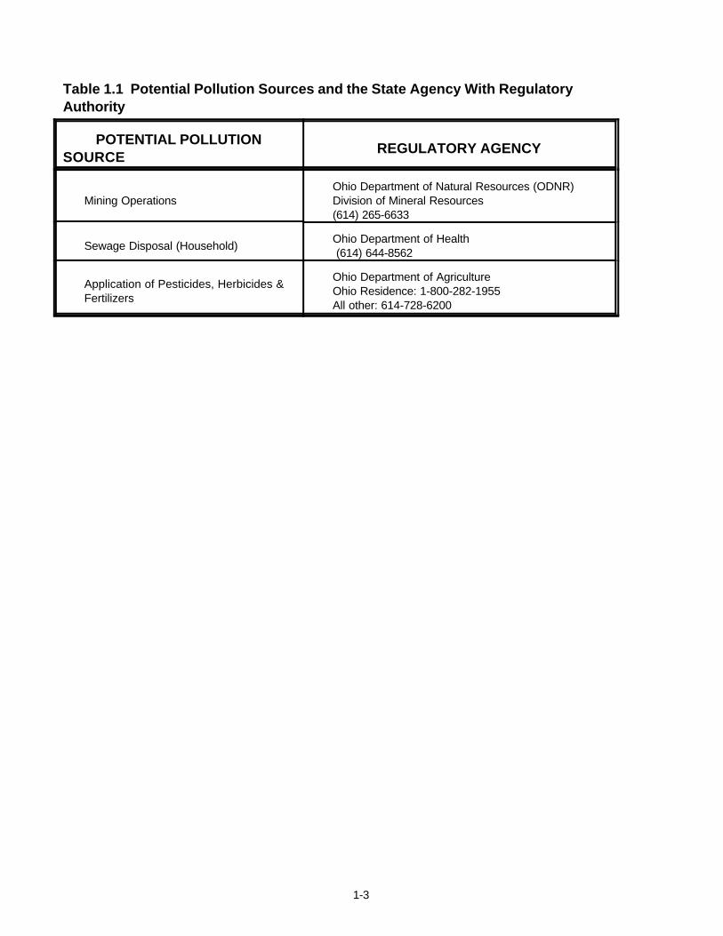
Table 1.1 Potential Pollution Sources and the State Agency With RegulatoryAuthority
POTENTIAL POLLUTIONSOURCE
REGULATORY AGENCY
1-3
Mining OperationsOhio Department of Natural Resources (ODNR)Division of Mineral Resources (614) 265-6633
Sewage Disposal (Household)Ohio Department of Health (614) 644-8562
Application of Pesticides, Herbicides &Fertilizers
Ohio Department of AgricultureOhio Residence: 1-800-282-1955All other: 614-728-6200
TECHNICAL GUIDANCE MANUAL FOR HYDROGEOLOGICINVESTIGATIONS AND GROUND WATER MONITORING
CHAPTER 2REGULATORY OVERVIEW
February 1995

-ii-
TABLE OF CONTENTS
CHAPTER 2: REGULATORY OVERVIEW
INTRODUCTION . . . . . . . . . . . . . . . . . . . . . . . . . . . . . . . . . . . . . . . . . . . . . . . . . . . . . . . . . . . . . . . . 2-1REGULATED HAZARDOUS WASTE FACILITIES . . . . . . . . . . . . . . . . . . . . . . . . . . . . . . . . . . . 2-1
PART A FACILITIES (INTERIM STATUS) . . . . . . . . . . . . . . . . . . . . . . . . . . . . . . . . . . . . . . . . 2-1PART B FACILITIES (PERMITTED FACILITIES) . . . . . . . . . . . . . . . . . . . . . . . . . . . . . . . . . . 2-2CORRECTIVE ACTIONS AT HAZARDOUS WASTE FACILITIES . . . . . . . . . . . . . . . . . . . . 2-2SOLID WASTE LANDFILLS . . . . . . . . . . . . . . . . . . . . . . . . . . . . . . . . . . . . . . . . . . . . . . . . . . . 2-3WASTEWATER FACILITIES . . . . . . . . . . . . . . . . . . . . . . . . . . . . . . . . . . . . . . . . . . . . . . . . . . . 2-4UNREGULATED HAZARDOUS WASTE SITES . . . . . . . . . . . . . . . . . . . . . . . . . . . . . . . . . . 2-4
REFERENCES . . . . . . . . . . . . . . . . . . . . . . . . . . . . . . . . . . . . . . . . . . . . . . . . . . . . . . . . . . . . . . . . 2-5

2-1
CHAPTER 2
REGULATORY OVERVIEW
Hydrogeologic investigations and ground water monitoring are mandated by state and federal laws,rules, and regulations. These requirements often govern the siting, operation, and closure of wastemanagement facilities or the remediation of contaminated sites. The purpose of this chapter is tosummarize Ohio EPA's authority to require ground water monitoring and/or hydrogeologicinvestigations at hazardous waste, solid waste, and wastewater facilities and unregulated sitesrequiring corrective actions.
REGULATED HAZARDOUS WASTE FACILITIES
The Ohio EPA's Division of Hazardous Waste Management (DHWM) has exclusive responsibilityfor the supervision, regulation, and enforcement of regulated hazardous waste facilities. Ohio'sprogram is based on Subtitle C of the Resource and Conservation and Recovery Act (RCRA) of1976 and is revised regularly to reflect changes in federal regulations. Ohio's rules, located inChapters 3745-49 through 3745-69 of the Ohio Administrative Code (OAC), are substantiallyequivalent to the federal regulations located in 40 CFR 260 to 270. Chapter 3745-51 of the OACidentifies those wastes that are subject to the rules.
The DHWM shares responsibility for permitting with the Ohio Hazardous Waste Facility Board(HWFB). The HWFB has responsibility for acting on applications for new facilities andmodifications of existing facilities, while the DHWM has responsibility for acting on applications forrevisions of existing facilities and permit renewals.
Facilities in Ohio can be categorized as follows: 1) Part A-permitted facilities that received aHazardous Waste Installation and Operation Permit from the HWFB (commonly known as interimstatus facilities; this includes facilities that were in operation prior to October 9, 1980 and haveapplied for a permit pursuant to OAC 3745-50), 2) facilities that have received a Part B permit fromthe HWFB or Ohio EPA (known as permitted facilities), 3) facilities that qualified for a permit by ruleunder provisions found in OAC 3745-50-40(C), 4) illegal or unpermitted facilities (treatment, storageor disposal of hazardous waste occurred after enactment of RCRA), and 5) facilities operatingunder an exemption that have yet to receive a final action on their permit application. The followingdiscussion identifies the major types of facilities for which ground water monitoring and/orhydrogeologic investigations are required.
PART A FACILITIES (INTERIM STATUS)
Until final administrative disposition of their permit applications, owners/operators of interim statusand illegal, unpermitted hazardous waste surface impoundments, landfills, and land treatment unitsare required to implement a ground water monitoring program capable of determining their facility'simpact on the underlying uppermost aquifer (OAC 3745-65-90 through 94). If any interim statusfacility does not receive a permit, it must be closed in a manner that complies with the standardsfound in OAC 3745-66-10 through 20. Ground water monitoring may be required to document that
1A SWMU is defined as "Any discernible unit at which solid or hazardous wastes have been placed atany time, irrespective of whether the unit was intended for management of solid or hazardous waste. Suchunits include any area at which hazardous waste or hazardous waste constituents have been routinely andsystematically released." (U.S.EPA, 1989)
2-2
standards have been met. If a facility cannot be "clean-closed," then it will have to be closed as alandfill and the owner/operator must comply with monitoring regulations contained in OAC 3745-65-90 through 94 [OAC 3745-68-10 (B) (2)].
PART B FACILITIES (PERMITTED)
Owners/operators of permitted hazardous waste surface impoundments, landfills, waste piles, andland treatment units must conduct a ground water monitoring program capable of determining thefacility's impact on the underlying uppermost aquifer (OAC 3745-54-90 through 99). Closures ofpermitted facilities that are not classified as surface impoundments, landfills, waste piles, or landtreatment units (such as treatment and storage facilities) must meet the standards of Chapter 3745-55-10 through 20. If a unit cannot be clean-closed, it must be closed as a landfill and compliancewith post-closure ground water monitoring requirements [OAC 3745-57-10 (B) (3)] must bedocumented.
CORRECTIVE ACTIONS
Ground water corrective action is mandated by OAC 3745-55-01, which addresses contaminationthat has migrated from a permitted hazardous waste surface impoundment, landfill, waste pile, orland treatment facility.
The Hazardous and Solid Waste Amendments (HSWA) to RCRA were enacted on November 8,1984. These amendments provide authority for U.S. EPA to require clean-up of releases from solidwaste management units (SWMUs)1. One of the major provisions of these amendments is Section3004(u), which requires corrective action for releases of hazardous waste or hazardous wasteconstituents from SWMUs at permitted treatment, storage, or disposal facilities (TSDs). Theobjective is to evaluate the nature and extent of any release and the measure(s) appropriate toprotect human health and the environment. Permits may contain schedules of compliance whencorrective action cannot be completed prior to issuance. Section 3004(v) authorizes U.S. EPA torequire corrective action beyond the facility boundary. Section 3008(h) provides U.S. EPA withauthority for facilities that are operating or that had operated under interim status. As of this date,the State of Ohio is not authorized to implement the corrective action provisions of the RCRA asamended by the HSWA. Ohio EPA currently serves as an agent of the U.S. EPA through mutualagreement.
According to the U.S. EPA, facilities subject to the HSWA encompass every TSD facility that had"interim status" within the federal definition of the term. The categories include: 1) those facilitiesfor which owner/operators submitted a Part A application to the U.S. EPA subsequent to theeffective date of the RCRA regulations that required any owner/operator who treated, disposed,stored, or accepted hazardous waste prior to November 1980 and requested to continue these
2-3
practices to submit the application; 2) those facilities for which owners/operators submitted a PartA permit application, in the category above, yet did not choose to submit a Part B application fora TSD, deciding instead to remain as a "generator" only, storing for less than ninety days; and 3)those facilities that held interim status and have since closed or ceased operation. These types,whether in operation or not, are subject to corrective action because they held federal interim statusat some point. The U.S. EPA has stated (Federal Register, Vol. 53, No. 122, June 24, 1988, p.23981) that it does not have authority to compel Subtitle C corrective action at facilities classifiedas protective filers. This type of facility includes generators, transporters or recyclers that have filedPart A permit applications for treatment or storage as a precautionary measure only.
Finally, facilities that have operated or are operating without interim status may be subject tocorrective action requirements. These facilities will be determined on a case-by-case basis as theyare discovered, and will most likely be addressed through an enforcement action under Section3008(h). The basis for application of 3008(h) to facilities without interim status is discussed in aDecember 16, 1985 internal memo to Regional Administrators (U.S.EPA, 1985).
SOLID WASTE LANDFILLS
The Ohio EPA's Division of Solid and Infectious Waste Management (DSIWM) has regulatoryauthority over solid waste landfills. Municipal landfills must meet Ohio's approved Subtitle D-basedrules, as amended in June 1994 (OAC Chapter 3745-27). The rules require that new landfillcapacity be designed to incorporate state-of-the-art technology. This means starting with a site thathas geologic characteristics that impede or restrict the movement of contaminants. Thesecharacteristics are enhanced by required engineering features. The rules detail siting criteria,leachate collection systems, surface water management systems, a cap system, ground watermonitoring/corrective action criteria, operational criteria, closure criteria, post-closure criteria, andfinancial assurance requirements for closure and post-closure activities.
In 1992, Ohio formally recognized that seven types of industrial wastes do not need to be regulatedas stringently as municipal solid waste. New rules (OAC Chapter 3745-30) went into effect onJanuary 13, 1992. The wastes are termed "residual wastes" in this Chapter. The rules provide forfour classes of landfills based on characterization of the specific waste streams. Class I residualwaste landfills must meet the criteria for municipal solid waste landfills. Requirements for siting,design, operations, closure, and post-closure at Class II and Class III landfills are not as stringentas the corresponding Class I requirements. Class IV residual waste landfills need to meet minimalsiting criteria and their owners are not required to perform ground water monitoring.
On June 1, 1994, Ohio promulgated separate rules (OAC 3745-29) for landfill facilities exclusivelydisposing of industrial solid waste not covered under the residual rules. These rules are similar toOAC 3745-27. While all municipal landfills in operation as of March 1, 1990 are subject to theground water monitoring requirements of OAC 3745-27-10 as of June 1, 1994, not all facilities aresubject to all of the provisions in the residual and industrial rules as of the rules' effective date. Newlandfills and expansions of existing landfills are under all of the residual and industrial rules. Existing

2-4
facilities are not evaluated under the siting or ground water monitoring provisions until a decisionon a mandated permit to upgrade to Ohio's approved rules is issued. Ground water monitoringprovisions are also required of existing facilities in an approved closure plan. Table 2.1summarizes the regulatory citations for residual waste landfill Classes I, II, and III; municipal solidwaste landfills; and industrial solid waste landfills relating to ground water monitoring, siting,corrective actions and hydrogeologic investigations.
Table 2.1. Regulations for ground water monitoring and hydrogeologic investigations atsolid waste landfills.
REQUIREMENT MUNICIPAL INDUSTRIALCLASS I, II and III
RESIDUAL
General ground watermonitoring program
OAC 3745-27-10 OAC 3745-29-10 OAC 3745-30-08
Hydrogeologicinvestigation report
OAC 3745-27-06 (C) (2) OAC 3745-29-06(C)(2) OAC 3745-30-05 (C) (3)
Siting criteria OAC 3745-27-07 (B) OAC 3745-29-07(H) OAC 3745-30-06 (B)
Corrective actions OAC 3745-27-10 (F) OAC 3745-27-10(F) OAC 3745-30-08 (F)
WASTEWATER FACILITIES
The Ohio EPA's Division of Surface Water (DSW) has regulatory authority over facilities subject toOhio's Clean Water Act (ORC 6111), including industrial and municipal wastewater treatment, non-toxic flyash, bottom ash, foundry sand, and coal pile runoff collection facilities. The Agency'sDivision of Environmental Financial Assistance (DEFA) provides loans for construction of municipalwastewater treatment facilities. State water pollution control regulations do not specify requirementsfor ground water monitoring. However, monitoring requirements for wastewater facilities aredetermined on a site-by-site basis, taking into account the location, engineering, and type of wasteto be treated.
UNREGULATED HAZARDOUS WASTE SITES
The Ohio EPA's Division of Emergency and Remedial Response (DERR) has authority overremedial activities conducted at unregulated hazardous waste sites. "Unregulated" sites are thosewhere the treatment, storage, or disposal of hazardous waste occurred prior to the enactment ofRCRA. Pursuant to the Comprehensive Environmental Response, Compensation, and Liability Act(CERCLA) of 1980, and as amended by the Superfund Amendments and Reauthorization Act

2-5
(SARA) of 1986, the U.S.EPA promulgated regulations that describe the technical requirementsof remedial projects. These regulations are known commonly as the National Contingency Plan(NCP) 40 CFR Part 300 et seq. Under Ohio law (ORC Sections 3734 and 6111), responsibleparties may be required to conduct hydrogeologic investigations and install and sample monitoringwells as part of a remedial project to define the presence or extent of contamination or to monitorthe progress of a selected remedy.
The Ohio General Assembly recently passed legislation, Sub. S.B 221, which creates a programunder ORC 3746 to allow people to voluntarily clean up contaminated (hazardous substances andpetroleum) property and receive a "Covenant Not to Sue" for the State of Ohio. Covenants willprovide volunteers and subsequent property owners with civil liability protection from having toperform additional cleanup work. All Covenants will be conditioned on cleanups meeting applicablestandards and remedies operating properly. An interim program began on September 28, 1994that allows some volunteers to receive covenants prior to the adoption of final rules by Ohio EPA.The Agency is required to have the rules in place by September 28, 1995.
REFERENCES
U.S.EPA. 1985. Internal Memo (12/16/85) to Regional Administrators. OSWER Directive9502.1985(09). Office of Solid Waste and Emergency Response. Washington, DC.
U.S.EPA. 1989. RCRA Facility Investigation Guidance, Interim Final. EPA/540-SW-89-031.Office of Solid Waste and Emergency Response. Washington, DC.

State of Ohio Environmental Protection Agency
Division of Drinking and Ground Waters
Technical Guidance Manual for Ground Water Investigations Chapter 3
Characterization of Site Hydrogeology
October 2006 Governor : Ted Strickland Director : Chris Korleski

TGM Chapter 3: Site Hydrogeology 3-ii Revision 1, October 2006
TECHNICAL GUIDANCE MANUAL FOR
GROUND WATER INVESTIGATIONS
CHAPTER 3
Characterization of Site Hydrogeology
October 2006
Revision 1
Ohio Environmental Protection Agency Division of Drinking and Ground Waters
P.O. Box 1049 50 West Town Street, Suite 700 Columbus, Ohio 43216-1049
Phone: 614-644-2752 http://www.epa.state.oh.us/ddagw/

TGM Chapter 3: Site Hydrogeology 3-iii Revision 1, October 2006
TABLE OF CONTENTS TABLE OF CONTENTS ................................................................................................... 3-iii ACKNOWLEDGMENTS ................................................................................................... 3-v CHANGES FROM THE FEBRUARY 1995 TGM .............................................................. 3-vi PRELIMINARY EVALUATIONS ....................................................................................... 3-1 FIELD METHODS TO COLLECT HYDROGEOLOGIC SAMPLES AND DATA ............... 3-6
DIRECT TECHNIQUES ............................................................................................... 3-6 Boring ...................................................................................................................... 3-6 Test Pits and Trenches ............................................................................................ 3-8 Pumping and Slug Tests ......................................................................................... 3-9 Environmental and Injected Tracers ........................................................................ 3-9 Ground Water Level Measurements ...................................................................... 3-10
SUPPLEMENTAL TECHNIQUES ............................................................................. 3-11 Geophysics ............................................................................................................ 3-11 Cone Penetration Tests ......................................................................................... 3-12 Aerial Imagery ....................................................................................................... 3-13
HYDROGEOLOGIC CHARACTERIZATION .................................................................. 3-13 STRATIGRAPHY ..................................................................................................... 3-13 DESCRIPTION AND CLASSIFICATION OF UNCONSOLIDATED MATERIALS ...... 3-14
Classification ......................................................................................................... 3-15 Particle Size, Particle Shape, and Packing ............................................................ 3-16 Color ...................................................................................................................... 3-16 Moisture Content ................................................................................................... 3-16 Consistency and Plasticity ..................................................................................... 3-17
DESCRIPTION AND CLASSIFICATION OF CONSOLIDATED MATERIALS ........... 3-18 FRACTURING ........................................................................................................... 3-19 GROUND WATER OCCURRENCE .......................................................................... 3-23
Flow Direction ........................................................................................................ 3-24 Horizontal Component...................................................................................... 3-25 Vertical Component and Interconnectivity ........................................................ 3-28 Seasonal and Temporal Effects ....................................................................... 3-28 Anthropogenic Effects ...................................................................................... 3-29 Potentiometric Maps ........................................................................................ 3-29
Hydraulic Gradient ................................................................................................. 3-32 Porosity/Effective Porosity ..................................................................................... 3-32 Hydraulic Conductivity ........................................................................................... 3-33
Estimation ............................................................................................ 3-35 Laboratory Tests ............................................................................................ 3-37 Field Tests ............................................................................................ 3-37
Intrinsic Permeability/Coefficient of Permeability ................................................... 3-39 Transmissivity ........................................................................................................ 3-40 Storage Coefficient, Specific Storage, And Specific Yield ..................................... 3-40 Flow Rate .............................................................................................................. 3-40
Calculation from Hydraulic Parameters ............................................................ 3-40 Field Determination of Flow Rate ..................................................................... 3-41
Saturated Zone Yield ............................................................................................. 3-41

TGM Chapter 3: Site Hydrogeology 3-iv Revision 1, October 2006
GROUND WATER USE DETERMINATION ................................................................... 3-42 PUBLICLY AVAILABLE RECORDS .......................................................................... 3-42 SURVEYS ................................................................................................................ 3-42 OTHER LINES OF EVIDENCE ................................................................................. 3-42
ANALYSIS AND PRESENTATION OF HYDROGEOLOGIC INFORMATION ................ 3-43 WRITTEN DESCRIPTION ......................................................................................... 3-44 RAW DATA ................................................................................................................ 3-45 CROSS SECTIONS .................................................................................................. 3-45 MAPS ........................................................................................................................ 3-45 METHODOLOGY ...................................................................................................... 3-46
REFERENCES ............................................................................................................... 3-47 APPENDIX I: Geophysical Methods ............................................................................. 3-55

TGM Chapter 3: Site Hydrogeology 3-v Revision 1, October 2006
ACKNOWLEDGMENTS
This guidance was developed by Ohio EPA’s Division of Drinking and Ground Waters (DDAGW). The following are acknowledged for the preparation of this document.
Lisa Koenig, DDAGW-CO, who had primary responsibility for researching and revising the original chapter and this updated version.
Chris Kenah and Sydney Poole, DDAGW-CO, DDAGW-CO, Michael Bondoc, DDAGW-CDO, Atiur Rahman, DDAGW-NEDO, Donald Vogel and Robin Roth,,DERR-CO, who provided input.
Jeff Patzke, DDAGW-CO, who serves as editor and project coordinator for the Technical Guidance Manual.
The Ohio EPA would also like to thank the numerous people who provided input during the development of the 1995 document. The comments and recommendations from the DDAGW-District Offices, and other Ohio EPA Divisions, state and federal agencies, private consultants, and regulated community were appreciated.

TGM Chapter 3: Site Hydrogeology 3-vi Revision 1, October 2006
PREFACE The subject of this document is techniques to characterize hydrogeology beneath a site. It is part of a series of chapters incorporated in Ohio EPA’s Technical Guidance Manual for Hydrogeologic Investigations and Ground Water Monitoring (TGM), which was originally published in 1995. DDAGW now maintains this guidance as a series of chapters rather than as an individual manual. These chapters can be obtained at http://www.epa.state.oh.us/ddagw/tgmweb.aspx. The TGM identifies technical considerations for performing hydrogeologic investigations and ground water monitoring at potential or known ground water pollution sources. The purpose of the guidance is to enhance consistency within the Agency and inform the regulated community of the Agency’s technical recommendations and the basis for them. In Ohio, the authority over pollution sources is shared among various Ohio EPA divisions, including the Emergency and Remedial Response (DERR), Hazardous Waste Management (DHWM), Solid and Infectious Waste (DSIWM), and Surface Water (DSW), as well as other state and local agencies. DDAGW provides technical support to these divisions. Ohio EPA utilizes guidance to aid regulators and the regulated community in meeting laws, rules, regulations and policy. Guidance outlines recommended practices and explains their rationale. Note that the term implies no enforcement authority. The Agency may not require an entity to follow methods recommended by this or any other guidance document. It may, however, require an entity to demonstrate that an alternate method produces data and information that meet the pertinent requirements. Ohio EPA recognizes that inflexibility in the language and/or interpretation of guidance can lead to the adoption of inappropriate measures, delay, and inefficiency. The procedures used to meet requirements usually should be tailored to the specific needs and circumstances of the individual site, project, and applicable regulatory program, and should not comprise a rigid step-by-step approach that is utilized in all situations.
TGM Chapter 3: Site Hydrogeology 3-vii Revision 1, October 2006
CHANGES FROM THE FEBRUARY 1995 TGM Changes to Chapter 3 are mainly organizational. A section was added to describe the field tools available to collect hydrogeologic data. The core of the document discusses the data that should be collected and the appropriate methods to do so. References were updated, in particular, the references to ASTM standards. Additional information has been added on:
geophysics (e.g., tables from chapter 11 were added to chapter 3), environmental isotopes, water level measurements, stratigraphy, construction of potentiometric maps, fractures, intrinsic permeability/coefficient of permeability, and ground water use determination.

TGM Chapter 3: Site Hydrogeology 3-1 Revision 1, October 2006
CHAPTER 3
CHARACTERIZATION OF SITE HYDROGEOLOGY Investigations of existing or potential ground water pollution sources should include an adequate characterization of site hydrogeology. Typically, an evaluation includes a three-dimensional assessment of the underlying geologic materials and the movement of ground water within the materials. This information is needed to assess whether ground water has been impacted by pollution sources, determine the extent of contamination, and determine whether contaminants have reached a receptor. The scope of an investigation should be based on it’s objectives, any regulatory requirements, and site-specific conditions. The following approach should be used:
Define the requirements and technical objectives. The requirements and objectives are dictated by the regulatory program. An entity may be evaluating the hydrogeology of an area to: 1) determine if it is compatible with its intended use; 2) ascertain the impact of a past, existing, or proposed activity on the ground water resources of the region; and/or 3) provide a basis for a site clean-up program. Project requirements and objectives should be discussed with the appropriate Agency representative prior to initiating studies.
Perform a preliminary evaluation. A preliminary evaluation is a comprehensive review of existing information, including regional and site-specific hydrogeologic data. The evaluation should be utilized to develop a preliminary conceptual model.
Collect site-specific hydrogeologic data. The results of the preliminary evaluation, along with project requirements and technical objectives, should be utilized to design the first phase of a site-specific investigation. Information gathered can be utilized to refine the conceptual model and assist in developing additional phases, if needed. In general, the characterization is considered complete when enough information has been collected to satisfy regulatory requirements and the potential pathways for contaminant migration have been defined and characterized. Prior to performing any field work, a site safety plan may need to be developed in accordance with the Occupational Safety and Health Administration (OSHA) requirements of 29 CFR 1910.120.
PRELIMINARY EVALUATIONS
Characterization should begin with a review of available regional and site-specific hydrogeologic information. Wastes or constituents of concern should also be investigated. This preliminary evaluation should serve as the basis for the conceptual model and field investigation. Information that may be gathered includes, but is not limited to:
Logs from private, public, industrial, agricultural, monitoring, oil, gas, and injection wells.

TGM Chapter 3: Site Hydrogeology 3-2 Revision 1, October 2006
Logs from building or quarry activities.
Records documenting local influences on ground water flow and use (e.g., on- or
off-site production wells, irrigation or agricultural use, river stage variations, and land use patterns, etc.).
Geologic and ground water data obtained from various reports for the area or region.
Topographic, geologic, soil, hydrogeologic, and geohydrochemical maps and aerial photographs.
Information may be obtained from the sources listed below. Division of Mineral Resource Management, Ohio Department of Natural Resources. (2045 Morse Road, Building H-2 & H-3, Columbus, Ohio 43229. Phone: 614-265-6633. Web address: http://ohiodnr.com/mineral/default/tabid/10352/Default.aspx). The Division of Mineral Resource Management is comprised of the following departments: Oil and Gas, Industrial Minerals, Coal Mining, Mine Safety, and Abandoned Mined Lands. The Department of Oil and Gas has oil and gas well completion records, which may provide general information on bedrock geology. Borehole geophysical logs may also be available. The Department of Industrial Minerals has hydrogeologic reports for new and existing quarry operations. This information may contain useful data on quarry geology and potential dewatering effects on local wells, including pumping test data and aquifer characteristics. In addition, each quarry must file an annual water withdrawal report with the ODNR Division of Water, which can provide an estimate of ground water pumpage. The Department of Coal Mining administers and regulates both surface and deep mines and has permits and hydrogeologic data on file, possibly in addition to what is available with the Division of Geological Survey. Division of Water, Ground Water, Ohio Department of Natural Resources (2045 Morse Road, Building E-3, Columbus, Ohio 43229. Phone: 614-265-6717. Web address: http://www.dnr.state.oh.us/tabid/3252/Default.aspx). The Ohio Department of Natural Resources (ODNR), Division of Water, Ground Water Resources Section, is responsible for the quantitative evaluation of ground water resources. Specific functions include ground water mapping, administration of Ohio's ground water well log and drilling report law, and special assistance to municipalities, industries, and the general public regarding local geology, well drilling and development, and quantitative problem assessment. Ground water availability maps have been published. These maps can be downloaded from the Division’s internet site or a paper copy can be ordered. The Division's file of logs include records for water supply and monitoring wells. Well logs are available on-line, or arrangements can be made to search the well log files. The Division is also involved in drafting pollution potential maps (often referred to as DRASTIC maps), which can be used in general planning. These maps are available on-line. Potentiometric surface maps are also available for some counties. These maps can be used for general planning. Other available information includes ground water reports and bulletins.

TGM Chapter 3: Site Hydrogeology 3-3 Revision 1, October 2006
Natural Resources Conservation Services (NRCS), United States Department of Agriculture (State Office Tower, 200 North High Street, Columbus, Ohio 43017. Phone: 614-644-6932). Web address: http://www.nrcs.usda.gov/. The NRCS (formerly Soil Conservation Services) provides leadership in a partnership effort to help private land owners and managers conserve their soil, water, and other natural resources. One source of information useful for preliminary investigations are the soil surveys. These maps illustrate major soil types and their agricultural and engineering attributes. The NRCS has digitized many of the surveys (Soil Survey Geographical (SSURGO) data base) and they are available on-line for almost all counties in Ohio. Maps also are available through the ODNR, Division of Soil and Water Conservation. Division of Soil and Water Conservation, ODNR (2045 Morse Road, Building B-3, Columbus, Ohio Phone: 614-265-6610. Web address: http://ohiodnr.com/tabid/8637/Default.aspx. The Division of Soil and Water Conservation, ODNR, has a variety of responsibilities, including performing investigations to determine soil characteristics, inventorying critical natural resource areas, and administering the Ohio Capabilities Analysis Program (OCAP), which provides mapping and analysis concerning geology and ground water availability. Aerial photographs can be obtained from this Division (614-265-6770). Division of the Geological Survey, ODNR , 2045 Morse Road, Building C, Columbus, Ohio 43229 Phone: 614-265-6576. Web address: http://ohiodnr.com/tabid/7105/Default.aspx.) The Division of the Geological Survey, ODNR, is responsible for the collection and dissemination of information relating to bedrock and surficial geology. Through mapping, core drilling, and seismic interpretation, the Survey compiles maps and inventories of bedrock and surficial materials and offers advice concerning mining-related issues. Published reports regarding bedrock and glacial geology are available for many counties. Additional information on bedrock geology is available from files of logs produced for oil and gas exploration. The USGS 7½ minute topographic maps are available from the Survey. These maps can provide basic information on spatial location of buildings (e.g., homes, schools, factories, etc.), roads and streams, surface elevations and topography, and general land use. These maps and reports can be ordered from the Division, and some are available on-line. United States Geological Survey (USGS), Ohio Water Science Center, 6480 Double Tree Avenue, 43229 Phone: 614-430-7700. Web address: http://oh.water.usgs.gov/index.html. The mission of the U.S.G.S., Water Resources Division is to provide the hydrologic information and understanding needed for the optimum utilization and management of the Nation's water resources for the overall benefit of the United States. A summary of the Survey's program in Ohio can be found in Open-File Report 93-458 (U.S.G.S., 1993). Responsibilities include collection of the basic data needed for determination and evaluation of the quantity, quality, and use of Ohio's water resources, conductance of analytical and interpretive water-resources appraisals describing the occurrence, availability, physical, chemical, and biological characteristics of surface water and precipitation, and implementation of similar appraisals associated with ground water. The U.S.G.S. publishes an annual series of reports titled "Water Resources Data-Ohio, Volume 1 and 2" in which the hydrologic data collected during each water year are presented. The U.S.G.S, National Center for Earth Resources Observation and Science (EROS) is the primary source for country-wide aerial photography.

TGM Chapter 3: Site Hydrogeology 3-4 Revision 1, October 2006
Ohio EPA (Lazarus Government Center, P.O. Box 1049, 50 West Town Street, Suite 700, Columbus, Ohio 43216-1049). Geologic or hydrogeologic information for a geographic area of concern can be obtained from Ohio EPA files if names of specific facilities/sites are known. Information on waste and/or material management history also can be obtained. Requests to conduct file searches need to be in writing and include site name, regulatory division, county, city, and address. The request should be addressed to the District Public Information Specialist (Figure 3.1). Requests for review of Central Office files should be addressed to Central Office, Legal Section (phone: 614-644-2037). Ohio Department of Transportation 1602 West Broad Street, Columbus OH 43223, Phone 614-275-1359. Web address: http://www.dot.state.oh.us/Pages/Home.aspx. Maps and photographs can be purchased from surveys conducted by the Office of Aerial Engineering. Other. The Ohio Department of Health (ODH) and each Ohio County Health department also have well completion logs and records of domestic wells. The county health departments may also have ground water contaminant data that are particular to their county. Local libraries may be a source of historical data and maps for an area.

TGM Chapter 3: Site Hydrogeology 3-5 Revision 1, October 2006
Figure 3.1 Ohio EPA Central Office and District Locations.

TGM Chapter 3: Site Hydrogeology 3-6 Revision 1, October 2006
FIELD METHODS TO COLLECT HYDROGEOLOGIC SAMPLES AND DATA This section covers various direct and supplemental field tools and methodologies used to characterize the subsurface materials and ground water conditions present within a given area by sampling or in-situ testing. The extent of characterization and specific methods used will be determined by the project objectives, regulatory requirements, and the data quality objectives of the investigations. Specific hydrogeologic information that should be collected and appropriate techniques (both field and laboratory) to collect the data are covered in the Hydrogeologic Characterization Section (Page 3-13). DIRECT TECHNIQUES All hydrogeologic site characterization efforts should include collection of subsurface samples. These can be collected from borings and/or trenches and are used to describe and classify the subsurface materials and define the stratigraphy. Other direct techniques include aquifer testing, environmental and injected tracers, and ground water level measurements. Boring/Coring The objectives of subsurface boring1 are to collect data that reflect site conditions and to begin to refine the conceptual model derived during the preliminary evaluation. Information about designing a subsurface soil/bedrock program is discussed below. Details on how to describe and classify the material is discussed on page 3-14. In general, most programs include collection of subsurface material samples using a coring device, split spoon sampler, thin wall sampler, and/or a continuous sampler. These samples are used to determine the physical and chemical properties of the subsurface materials. The type of drilling equipment and sampling methods depends on the material, nature of the terrain, intended use of the data, depth of exploration, and prevention of cross-contamination. Detailed information pertaining to drilling and sampling is covered in Chapter 6. The location and spacing of borings necessary depends on subsurface complexity and on the importance of soil and rock continuity to the project design. In general, the density should be greater when characterizing geology that is more complex. Table 3.1 lists factors that should be considered. If existing data do not define site stratigraphy, additional boreholes and ancillary investigative techniques should be implemented. The number and placement of additional borings should be based on the preliminary conceptual model, refined with data obtained from the completed borings and other investigatory techniques. The locations of individual borings should depend on site hydrogeology, geomorphic features, spatial location of waste (or suspected waste), and anthropogenic (human-made) impediments such as underground utility lines. Boreholes should not be installed through waste material; however, in some instances this is unavoidable. Authorization from Ohio
1Borings not to be converted into wells must be properly sealed (See Chapter 9).
TGM Chapter 3: Site Hydrogeology 3-7 Revision 1, October 2006
EPA is required before drilling through waste. (ORC 3734.02(H))2. The applicable regulatory program should be contacted for appropriate authorization. The proper sampling interval and depth also depend on subsurface complexity. Exploration should be deep enough to identify all strata that might be significant in assessing the environmental conditions. At a minimum, initial borings should be sampled continuously. Once control has been established, the continuous approach may no longer be necessary. It should be noted that the proper interval may not be constant and may depend on the target zone(s) of interest. Care should be taken when drilling into confining units so that the borehole does not create a conduit for migration of contaminants between hydraulically separated saturated zones. Two approaches for drilling through confining layers should be considered:
Drill initially on the site perimeter (in less contaminated or uncontaminated areas). These borings could penetrate the confining zone to characterize deeper units. At a minimum, boreholes upgradient of the source could be drilled through the possible confining layer to characterize site geology. The appropriateness of this approach should be evaluated on a site-specific basis.
Drill using techniques (e.g., telescoped casing) that minimize potential cross-contamination, particularly from dense non-aqueous phase liquids (DNAPLs). Telescoped casing involves drilling partially into a confining layer, installing an exterior casing, sealing the annular space in the cased portion of the borehole, and drilling a smaller diameter borehole through the confining layer ( See Chapter 6).
2The Ohio Revised Code (ORC) states that: No person shall engage in filling, grading, excavating, building, drilling or mining on land where a hazardous waste facility, or solid waste facility was operated without prior authorization from the Director.
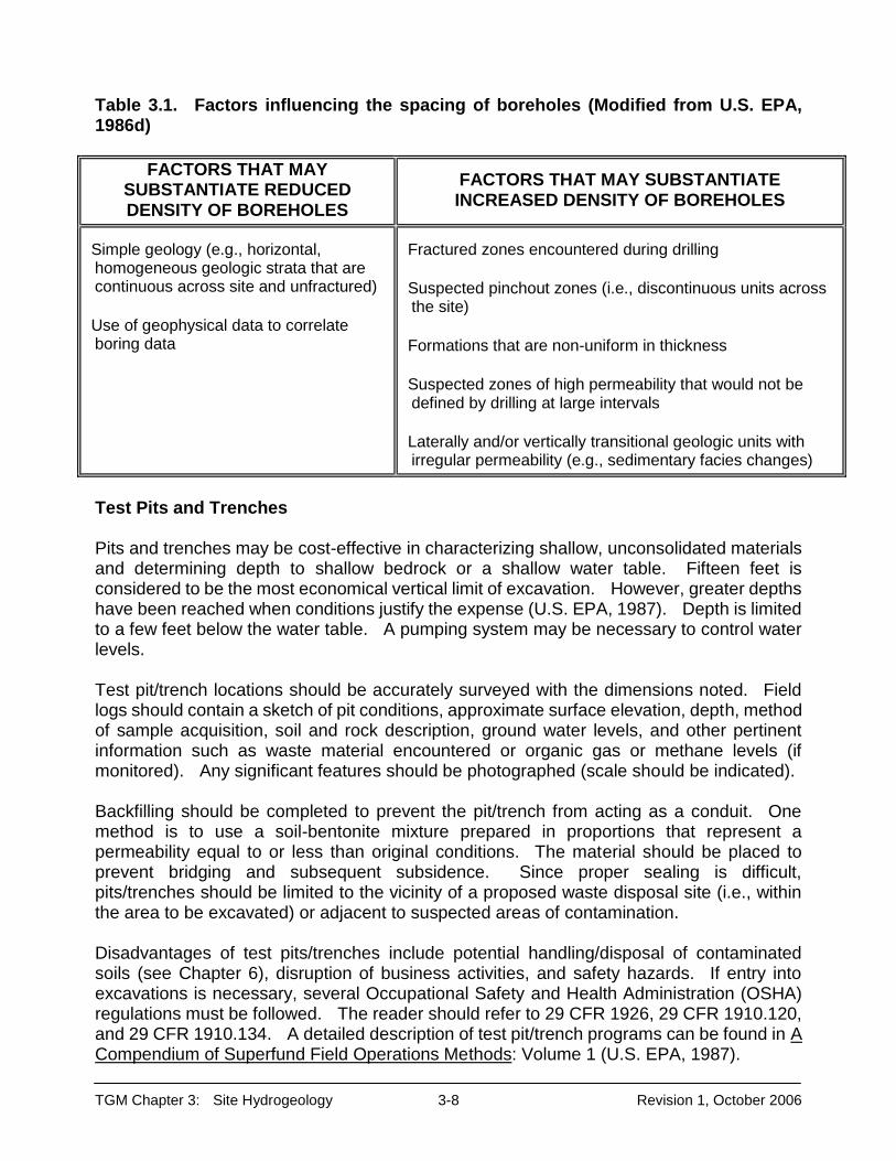
TGM Chapter 3: Site Hydrogeology 3-8 Revision 1, October 2006
Table 3.1. Factors influencing the spacing of boreholes (Modified from U.S. EPA, 1986d)
FACTORS THAT MAY SUBSTANTIATE REDUCED DENSITY OF BOREHOLES
FACTORS THAT MAY SUBSTANTIATE INCREASED DENSITY OF BOREHOLES
Simple geology (e.g., horizontal, homogeneous geologic strata that are continuous across site and unfractured) Use of geophysical data to correlate boring data
Fractured zones encountered during drilling Suspected pinchout zones (i.e., discontinuous units across the site) Formations that are non-uniform in thickness Suspected zones of high permeability that would not be defined by drilling at large intervals Laterally and/or vertically transitional geologic units with irregular permeability (e.g., sedimentary facies changes)
Test Pits and Trenches Pits and trenches may be cost-effective in characterizing shallow, unconsolidated materials and determining depth to shallow bedrock or a shallow water table. Fifteen feet is considered to be the most economical vertical limit of excavation. However, greater depths have been reached when conditions justify the expense (U.S. EPA, 1987). Depth is limited to a few feet below the water table. A pumping system may be necessary to control water levels. Test pit/trench locations should be accurately surveyed with the dimensions noted. Field logs should contain a sketch of pit conditions, approximate surface elevation, depth, method of sample acquisition, soil and rock description, ground water levels, and other pertinent information such as waste material encountered or organic gas or methane levels (if monitored). Any significant features should be photographed (scale should be indicated). Backfilling should be completed to prevent the pit/trench from acting as a conduit. One method is to use a soil-bentonite mixture prepared in proportions that represent a permeability equal to or less than original conditions. The material should be placed to prevent bridging and subsequent subsidence. Since proper sealing is difficult, pits/trenches should be limited to the vicinity of a proposed waste disposal site (i.e., within the area to be excavated) or adjacent to suspected areas of contamination. Disadvantages of test pits/trenches include potential handling/disposal of contaminated soils (see Chapter 6), disruption of business activities, and safety hazards. If entry into excavations is necessary, several Occupational Safety and Health Administration (OSHA) regulations must be followed. The reader should refer to 29 CFR 1926, 29 CFR 1910.120, and 29 CFR 1910.134. A detailed description of test pit/trench programs can be found in A Compendium of Superfund Field Operations Methods: Volume 1 (U.S. EPA, 1987).

TGM Chapter 3: Site Hydrogeology 3-9 Revision 1, October 2006
Pumping and Slug Tests Pumping and Slug tests are used to define the hydraulic characteristics of ground water zones and confining layers that lie above or below. These properties may also be needed to predict the ground water flow rate and design effective ground water remediation systems. Slug tests can provide information about the hydraulic conductivity of a layer. Pumping tests can provide information on hydraulic conductivity, interconnectiveness between ground water zones, heterogeneity, and boundary conditions. One drawback of long-term pumping tests is the volume of water that is discharged. Information on how to design pumping and slug tests is provided in Chapter 4. Environmental and Injected Tracers A tracer test is a field method used to quantify selected hydrogeologic characteristics of a ground water zone (Weight and Soderegger, 2000). A tracer is matter or energy carried by ground water that will indicate the direction and movement of water and potential contaminants that may be transported (Davis et al., 1985). Tracers can be naturally-occurring, such as heat carried by hot-spring waters; globally-produced from anthropogenic sources, such as an above-ground detonation test; or intentionally injected3, such as dyes. Naturally-occurring and globally-produced types often are referred to as environmental tracers. If sufficient information is collected, tracers may be used to determine hydraulic conductivity (K), porosity, dispersivity, chemical distribution coefficients, flow direction, flow rate, sources of recharge, and ground water age. A tracer should have a number of properties to be useful. It should be non-reactive, relatively inexpensive, and easily sampled, analyzed, and detected. Any injected tracer should be non-toxic and should be used with careful consideration of possible health effects. Isotopes, which are atoms of the same element that differ in mass because of a difference in the number of neutrons in the nucleus, serve as valuable tracers. The naturally-occurring elements give rise to more than 1,000 stable and radioactive isotopes, commonly referred to as environmental isotopes. These can be used to identify the origin of ground water, determine its relative age (i.e., length of time it has been out of contact with the atmosphere), and determine if saturated zones are interconnected. This can be important when trying to determine how long it may take a potential contaminant to reach a ground water zone or receptor. Age-dating shows which wells draw more recently recharged ground water and, therefore, may be more susceptible to contamination from the surface. Older water may be less contaminated because it has either been shielded from contact with pollutants or has had more time for natural processes to reduce or eliminate contamination.
3If fluids are injected into the subsurface, a Class V well operating permit may be required. Ohio EPA, Division of Drinking and Ground Waters, Underground Injection Control Unit (UIC) has jurisdiction over review and issuance of these permits. Under certain conditions, it may be possible to apply for and receive an exemption from the formal permitting process for injection wells used for hydraulic testing. If you have any questions concerning Class V wells, please contact the Ohio EPA-DDAGW, UIC unit. http://www.epa.state.oh.us/portals/28/documents/uic/webpageinventory.pdf.

TGM Chapter 3: Site Hydrogeology 3-10 Revision 1, October 2006
All dating techniques have limitations. Greater confidence in apparent age will be realized as multiple dating techniques are applied to the same sample. Isotopes and/or isotope ratios that may assist in evaluating the ground water include:
Tritium H3, which is used to determine if ground water was recharged prior to 1954 or after 1954.
Oxygen-18/oxygen -16 ration (18O/16O), which indicates if ground water is pre-Holocene or post-Holocene in age.
Relative fractions of deuterium (δH2) and oxygen-18 (δ18O) (Fetter, 2001). Where glacial tills are wide-spread, vertical profiles of δH2 and δ18O in pore waters are valuable natural isotopes that yield independent information on hydraulic properties and solute transport mechanism.
Carbon -14 (14C), which is used to estimate the relative age of ground water.
Titium (3H)/Helium-3 (3He) ratio. When 3He is due to decay of 3H and can be separated from that due to other sources, parent-daughter ratios enable accurate estimations of ground water age. Such information can be useful to estimate ground water residence and flow velocities (Solomon and Cook, 2000).
Chlorofluorocarbons (CFCs) Chlorofluorocarbons are stable, synthetic, halogenated alkanes, developed in the early 1930's as an alternative to ammonia sulphur dioxide refrigeration. They provide tracer and dating tools of younger water (50 year time scale.) Additional information on the application of chlorofluorocarbons can be found in Plummer and Busenberg (2000).
The complexities of natural systems together with the use criteria for tracers makes selection and use almost as much of an art as it is a science (U.S.EPA, 1991). The potential chemical and physical behavior of the tracer in the ground water must be understood. The type of medium and flow regime should also be considered. It is beyond the scope of this document to detail the proper use, selection, and design of tracers. Sources of information include: Davis et al. (1985), Alley (1993), Kazemi et al., (2006), Cook and Herczeg (editors, 2000) and the U.S.G.S. National Research Program http://water.usgs.gov/nrp/groundwater.html. Ground Water Level Measurements Water level measurements in wells are needed to: determine ground water flow and hydraulic gradients, interpret the amount of water available for withdrawal, and determine the effects of natural and anthropogenic (human-induced) influences on flow. Water levels can be collected manually or by continuous recorders. In addition to measurements from wells, information from springs, seeps, rivers, ponds and lakes may also be useful if they are shown to be hydraulically connected to the ground water zone being studied. The number and location of observation wells are critical to any water level data program. Selection of the location and depth should be based on hydrogeolgic/geologic

TGM Chapter 3: Site Hydrogeology 3-11 Revision 1, October 2006
characteristics of the area, physical boundaries, anthropogenetic influences and contaminant characteristics. Areas with multiple ground water zones may necessitate clusters of wells. Manual water level measurements are generally obtained with electrical probes or transducers and are a component of any ground water sampling program (See Chapter 10: Ground Water Sampling). When measuring manually, water levels from all wells should be taken in as short a time as possible. Influences, such as recharge from precipitation, barometric pressure changes, water withdrawal, artificial recharge (e.g., injection wells, leakage around a poorly sealed well) and heavy physical objects that compress the sediments(e.g., passing train), may change the water level in wells and affect the interpretation of ground water flow. However, often wells within a study area do not change significantly in a short time. It is often necessary to monitor the continuous fluctuation of water. Continuous measurements methods include: a mechanical float recording system, electromechanical iterative conductance probes connected to chart recorders, and tranducers with data loggers (Dalton et al., 2006). ASTM 6000 provides graphical and tabular methods for presenting ground water level information. SUPPLEMENTAL TECHNIQUES Supplemental techniques such as geophysics, cone penetration tests, and aerial imagery can be used to help guide and implement a boring program and assist in defining site hydrogeology. Use of these techniques can be cost-effective, as they may reduce the number of borings necessary. Geophysics Geophysics may be used to augment direct field methods or guide their implementation. Measurements supplement borehole and outcrop data and assist in the interpolation between boreholes. Geophysics can also be useful in identifying surface drilling hazards and contamination. Techniques can be categorized as either surface or borehole. Surface methods are generally non-intrusive. Borehole methods require that wells or borings exist so that tools can be lowered into the subsurface. Direct push (DP) technology probes have been fitted with sensors and can provide information rapidly (See Chapter 15: Use of Direct Push Technologies for Soil and Ground Water Sampling). Surface techniques can provide information on depth to bedrock, types and thicknesses of geologic material, presence of fracture zones and solution channels, structural discontinuities, and depth to the water table. They are also useful in locating drilling hazards (e.g., buried drums and pipelines). Types of surface geophysical techniques include: ground penetrating radar, electromagnetic induction, electrical resistivity, seismic refraction, seismic reflection, and magnetic surveys.
TGM Chapter 3: Site Hydrogeology 3-12 Revision 1, October 2006
Borehole techniques can be used to obtain information on material type, stratigraphy, formation and aquifer properties, ground water flow, borehole fluid characteristics, contaminant characteristics, and borehole/casing conditions. They may indicate areas of high porosity and hydraulic conductivity, ground water flow rates and direction, subsurface stratigraphy, lithology of bedrock units, and chemical and physical characteristics of ground water (Repa and Kufs, 1985). Borehole methods include nuclear logs (natural gamma, gamma-gamma, neutron-neutron, non-nuclear logs, and physical logs (temperature, fluid conductivity, fluid flow and caliper.) This chapter does not describe the various geophysical methods, however, a list of various methods helpful to characterize site hydrogeology is contained in Appendix I, along with techniques that may help identify contaminants and contaminant sources (buried drums, pipelines, etc). A description of various methods for identifying subsurface conditions and contaminant sources can be found in Chapter 11. All geophysical methods require site conditions that provide contrast in the subsurface properties being measured. Depending on the method, implementation may be affected by interferences such as metal fences, powerlines, FM radio transmissions or ground vibrations. Data collected and interpreted from geophysical surfaces require skilled personnel familiar with the principles and limitations of the method being used (ASTM, D5730-02). Cone Penetration Tests Cone penetration testing (CPT) is applicable where formations are uncemented and unlithified; free from impenetrable obstructions such as rock ledges, hardpans, caliche layers, and boulders; and conducive to penetration with minimal stress to the testing equipment (Smolley and Kappmeyer, 1991). The technique consists of advancing a mechanical or electronic rod to determine the end-bearing and side friction components of resistance to penetration (ASTM D3441-05, ASTM D5778-95). These two parameters typically are different for coarse-grained and clayey soils, making the CPT a particularly useful tool for defining and correlating the occurrence of sands and gravels versus clays and silts (Smolley and Kappmeyer, 1991). Mechanical cone penetrometers are addressed in ASTM D3441-05, while electronic cone penetrometers are addressed in ASTM D5778-95. The mechanical penetrometer operates incrementally using a telescoping tip, which results in no movement of the push rod. Electronic cone penetrometers use force transducers located in a non-telescoping penetrometer tip to measure penetration resistance. Other sensors--such as piezometric head transducers, pH indicators, and detectors for petroleum hydrocarbons--may also be included in the cone to provide additional information. At sites where the technique is applicable, CPT surveys can provide a continuous vertical profile of subsurface stratigraphy and indications of permeability. In all cases, the data should be compared with information from borings and geologic material sampling. Additional information on the use of CPT for environmental site investigations is presented in U.S. EPA (1997).
TGM Chapter 3: Site Hydrogeology 3-13 Revision 1, October 2006
Aerial Imagery Aerial imagery can be used to help: 1) identify rock and surface soil types, geomorphological features, and the nature and extent of joint and fault patterns; 2) approximate stream flow, evapotranspiration, infiltration, and runoff values; and 3) map topographic features such as streams, seeps, and other surface waters not readily apparent from ground level (Repa and Kufs, 1985). Comparing old and new topographic maps and aerial photographs can help ascertain changes over time such as those caused by cut and fill activities, drainage alteration, and land use (Benson, 2006). Vegetative stress identified in aerial imagery may indicate the location of a contaminant plume. Aerial imagery can be used for fracture analysis. Fracture traces are surface expressions of joints concentrations of faults. Fractures may provide pathways for ground water and contaminants. The greatest yields may be located at the intersection of two fracture traces. Therefore, fracture trace analysis may be help identify appropriate boring and monitoring well locations. Fracture trace analysis is covered on page 3-23. Aerial photographs may be obtained from the ODNR, Division of Soil and Water Conservation (614-265-6670) or from the U.S. Department of Agriculture, Agriculture Stabilization and Conservation Service (ASCS) offices in each county. They may also be available through the Ohio Department of Transportation, Office of Aerial Engineering. Documentation of analysis of aerial photographs should include source, date, and type of photograph. Information on the use of aerial photography can be found in Nielsen et al. (2006).
HYDROGEOLOGIC CHARACTERIZATION A proper evaluation of site hydrogeology should include, but not be limited to, identification of the lateral and vertical extent of subsurface materials, the type of materials, and the geological influences that may control ground water flow (e.g., high permeability zones, fractures, fault zones, fracture traces, buried stream deposits etc.), and the occurrence and use of ground water. As indicated above, direct information is collected through borings, test pits, and field and laboratory identification of subsurface materials. Supplemental information (e.g., geophysical data) can be used to augment the direct methods or to guide their implementation, but should not be used as a substitute. STRATIGRAPHY Stratigraphy is the study of the formation, composition, sequence and correlation of unconsolidated materials and rock. It includes formation designation, age, thickness, areal extent, composition, sequence, and correlation. In effect, stratigraphy defines the geometric framework of the ground water flow system. Therefore, knowledge of the local stratigraphy is necessary to define the hydrogeologic framework and identify pathways of chemical migration and extent of migration. Necessary determinations include zones that may restrict movement of ground water (confining zones) and zones that enhance ground water movement.
TGM Chapter 3: Site Hydrogeology 3-14 Revision 1, October 2006
Existing information such as driller’s logs and regional information can provide information on stratigraphy. This information may be helpful in designing a site-specific drilling program. Sample collection from borings and cores are needed to determine whether the subsurface layers have the ability to transmit water or prohibit the movement of water by serving as a confining layer. Geophysical methods can be used to direct or augment the characterization of stratigraphy. Thick, continuous layers of unfractured clay, fine silt, or shale may retard flow. They are generally identified by observing and testing the material from boreholes. Vertical hydraulic conductivity testing is conducted to assess the ability of these layers to retard flow vertically. Methods to determine hydraulic conductivity are discussed on page 3-33. Correlation between boreholes is necessary to assure that the layer is laterally continuous across the site. Testing of the fraction of organic carbon and/or cation exchange capacity is often done to assess a layer’s ability to retard the migration of contaminants (See Table 3.2). Characteristics of zones that enhance ground water movement include permeability; depth; thickness; lateral and vertical extent; flow direction, including temporal and seasonal fluctuations; flow rate; interconnection to surface water; and anthropogenic influences. DESCRIPTION AND CLASSIFICATION OF UNCONSOLIDATED MATERIALS Both laboratory and field testing are necessary for an accurate description and classification of unconsolidated materials. Characteristics that are discussed in this section include particle size, moisture content, color, plasticity, and consistency. A discussion on permeability/hydraulic conductivity and porosity can be found on page 3-32. Effort should be made to ensure quality and consistency in field descriptions. Other physical properties that may be useful include dry strength, dilatancy, toughness, and cementation. Criteria for describing these are given in ASTM 2488-00. If the goal of an investigation is to determine if subsurface material will attenuate contaminant migration, bulk density, cation exchange capacity, soil pH, and mineral content may need to be determined. Table 3.2 gives references and analytical methods for these parameters.
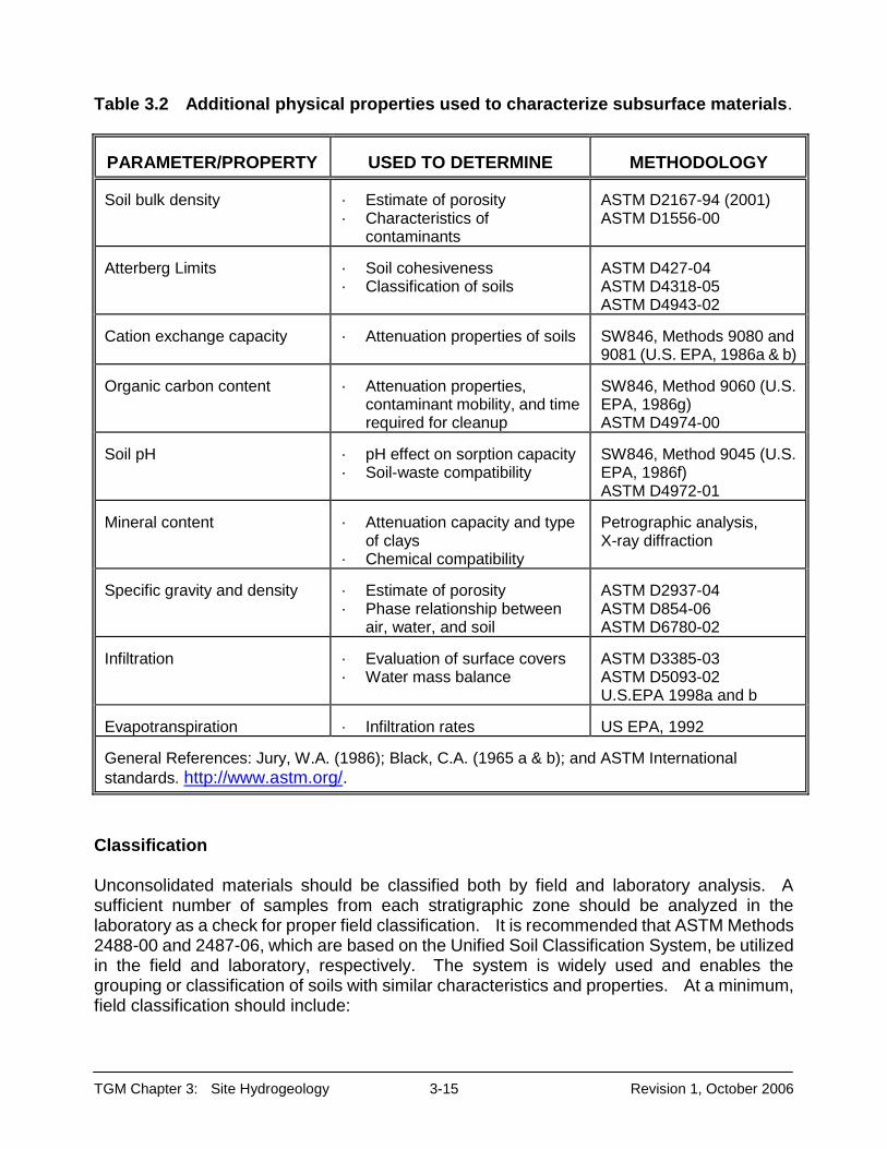
TGM Chapter 3: Site Hydrogeology 3-15 Revision 1, October 2006
Table 3.2 Additional physical properties used to characterize subsurface materials.
PARAMETER/PROPERTY
USED TO DETERMINE
METHODOLOGY
Soil bulk density
· Estimate of porosity · Characteristics of
contaminants
ASTM D2167-94 (2001) ASTM D1556-00
Atterberg Limits
· Soil cohesiveness · Classification of soils
ASTM D427-04 ASTM D4318-05 ASTM D4943-02
Cation exchange capacity
· Attenuation properties of soils
SW846, Methods 9080 and 9081 (U.S. EPA, 1986a & b)
Organic carbon content
· Attenuation properties,
contaminant mobility, and time required for cleanup
SW846, Method 9060 (U.S. EPA, 1986g) ASTM D4974-00
Soil pH
· pH effect on sorption capacity · Soil-waste compatibility
SW846, Method 9045 (U.S. EPA, 1986f) ASTM D4972-01
Mineral content
· Attenuation capacity and type
of clays · Chemical compatibility
Petrographic analysis, X-ray diffraction
Specific gravity and density
· Estimate of porosity · Phase relationship between
air, water, and soil
ASTM D2937-04 ASTM D854-06 ASTM D6780-02
Infiltration
· Evaluation of surface covers · Water mass balance
ASTM D3385-03 ASTM D5093-02 U.S.EPA 1998a and b
Evapotranspiration
· Infiltration rates
US EPA, 1992
General References: Jury, W.A. (1986); Black, C.A. (1965 a & b); and ASTM International standards. http://www.astm.org/.
Classification Unconsolidated materials should be classified both by field and laboratory analysis. A sufficient number of samples from each stratigraphic zone should be analyzed in the laboratory as a check for proper field classification. It is recommended that ASTM Methods 2488-00 and 2487-06, which are based on the Unified Soil Classification System, be utilized in the field and laboratory, respectively. The system is widely used and enables the grouping or classification of soils with similar characteristics and properties. At a minimum, field classification should include:

TGM Chapter 3: Site Hydrogeology 3-16 Revision 1, October 2006
Particle Size, Particle Shape, and Packing Sedimentary deposits are classified broadly into gravel, sand, silt, and clay. Particle size, including identification of the major and minor components using descriptive terms such as trace, little, some, and mostly (see Table 3.3). Particle size, shape, and packing can influence water storage, porosity, and flow. Highly angular and irregularly shaped, non-cemented grains tend to result in a greater porosity than smooth, regularly shaped grains, although the difference may be slight. Particle size generally is determined by visual observation and in the laboratory by sieve analysis (particles larger than 75 micrometers) or use of a hydrometer (particles less than 75 micrometers) (ASTM 422-63). Range distribution of particle size can be used to estimate permeabilities, design monitoring wells, and enable better stratigraphic interpretation.
Table 3.3. Relative percentage of particles by visual observation (ASTM D2488-00).
PARTICLE AMOUNT
PERCENTAGE
trace
less than 5 %
few
5 to 10 %
little
15-25%
some
30 to 45 %
mostly 50 to 100 %
Color Color can help identify materials of similar origin. Many minerals are light gray, but soils can be red, yellow, brown, or black. Color changes can indicate contamination, although variations also can be caused by natural conditions such as changes in the percent of organic matter content. Mottling may indicate impeded drainage or a seasonal high water table. Brown or orange-brown colorization can indicate oxidizing conditions (above the water table), while gray can indicate a reducing environment (below the water table). The identification should be standardized by use of a color chart (e.g., Munsell ® Color Chart) for two reasons: 1) a color often is described differently by different persons, and 2) a given color appears differently when seen next to other colors (e.g., gray can appear bluish when next to orange or brown earth colors) (Compton, 1985). Moisture Content Relative moisture content should be determined in the field, with the material classified as dry, moist, or wet. Table 3.4 recommends general criteria (ASTM D2488-00). The actual moisture content is the ratio of the weight of water to the total weight of solid particles. It is

TGM Chapter 3: Site Hydrogeology 3-17 Revision 1, October 2006
critical when determining the adequacy of a lining material or conducting vadose zone monitoring and, in some cases, when designing remedial methods. Table 3.4 Criteria for describing moisture content (ASTM D2488-00).
DESCRIPTION
CRITERIA
dry
absence of moisture, dry to the touch
moist
damp, no visible water
wet
visible free water, usually soil is below the water table
Laboratory methods for determining moisture content include thermal (ASTM D2216-05, D4959-00), gravimetric, chemical extraction, mechanical extraction (ASTM D1557-91), and immersion and penetration (ASTM D3017-05). Field methods include electromagnetic, electrothermal, and nuclear. Detailed procedures and discussions are available in the literature (Morrison, 1983). The procedures should be evaluated to determine which is most appropriate for any particular situation. Consistency and Plasticity Consistency is the relative ease with which soil can be deformed. It can be determined by blow counts from split-spoon sampling4 or with a pocket penetrometer. If a penetrometer is not available, consistency can be approximated according to Table 3.5.
Table 3.5 Criteria for describing consistency (ASTM-2488-00). DESCRIPTION
CRITERIA
Very Soft
Thumb will penetrate soil more than 1 in. (25 mm)
Soft
Thumb will penetrate soil about 1 in. (25 mm)
Firm
Thumb will indent soil about 1/4 in. (6 mm)
Hard
Thumb will not indent soil but readily indented with thumbnail
Very hard
Thumbnail will not indent soil
Plasticity is the property of soil or rock that allows it to be deformed beyond the point of recovery without cracking or exhibiting appreciable change in volume. The relative plasticity can be estimated in the field by using Table 3.6.
4A standard split spoon sampler is driven by a 140 lb hammer falling 30 inches. The number of blows required to drive the sampler 6 inches is the standard penetration resistance or blow counts, N.

TGM Chapter 3: Site Hydrogeology 3-18 Revision 1, October 2006
Plasticity and consistency also can be described by Atterberg Limits. Atterberg Limits are defined as indices of workability or firmness of an artificial mixture of soil and water as affected by water content (Holtz and Kovacs, 1981). The indices include the liquid limit, plastic limit, and the plastic index. The liquid limit (upper plastic limit) is the point at which soil becomes semi-fluid. The plastic limit (or lower plastic limit) is the water content at which soil begins to crumble when rolled into a thread (i.e., lower limit to which it can be deformed without cracking). The plastic index is the difference between the liquid limit and the plastic limit and is an indication of plasticity. Atterberg Limits are used widely in soil classification systems and for evaluation of clay liners. They can be determined by ASTM Methods D4318-05, D4943-02, and D427-04. Table 3.6 Criteria for describing plasticity (ASTM-2488-00). DESCRIPTION
CRITERIA
Nonplastic
A ½-in. (13-mm) thread cannot be rolled at any water content.
Low
The thread can barely be rolled and the lump cannot be formed when drier than the plastic limit.
Medium
The thread is easy to roll and not much time is required to reach the plastic limit. The thread cannot be rerolled after reaching the plastic limit. The lump crumbles when drier than the plastic limit.
High
It takes considerable time rolling and kneading to reach the plastic limit. The thread can be rerolled several times after reaching the plastic limit. The lump can be formed without crumbling when drier than the plastic limit.
Other methods can be used as long as the system is identified, described adequately, and used consistently. At a minimum, the method should account for all particle sizes encountered, color, relative moisture content, and consistency. If fractures are observed, they should be noted and described. If possible, the sedimentary environment should be identified. In general, unconsolidated sediments within Ohio can be described as glacial, lacustrine, fluvial, colluvial, residual, or eolian. DESCRIPTION AND CLASSIFICATION OF CONSOLIDATED MATERIALS The uppermost consolidated units (bedrock) in Ohio are sedimentary and generally consist of carbonate rock, sandstone, shale or coal that ranges in age from Ordovician to Permian. Distinctive characteristics that are influential with respect to ground water movement include porosity, permeability, fracturing (including stress release), bedding, and solution weathering (karst). Porosity and hydraulic conductivity measurements are discussed later in this chapter. Fractures can be identified by a boring program and fracture trace analysis. Bedding plane spacing, strike, and dip should be indicated. Prominent bedding planes should be distinguished from banding due to color or textural variation. An attempt should be made to determine the formation name to assess regional characteristics.

TGM Chapter 3: Site Hydrogeology 3-19 Revision 1, October 2006
The competence of the consolidated materials can be described by the Rock Quality Designation (RQD). The RQD is calculated by measuring the total length of all competent core pieces greater than four or more inches, dividing it by the length of the core run, and multiplying by 100. In general, the higher the RQD, the higher the integrity. Table 3.7 lists RQD and a description of rock quality (Ruda et al.,2006).
Table 3.7 RQD
RQD Description of Rock Quality
0-25
Very Poor
50
Poor
75
Fair
90
Good
100
Excellent
FRACTURING Fractures are breaks in geologic material due to stress. As they play an important role in the movement of water and contaminants through bedrock and unconsolidated materials, their presence needs to be identified and evaluated. However, the mere presence of fractures may not be enough to allow for ground water flow. Aspects of fractures that may need to be evaluated to determine if contribute or control ground water flow include: orientation, density, depth, aperture opening, and connectivity of the fractures. Clayey soils are generally assumed to act as low permeability confining units, providing acceptable isolation distances to underlying ground water resources that could be impacted by contaminant sources. However, if fractures and other macropores are not adequately evaluated and accounted for, the hydraulic conductivity of clayey soils may be underestimated by as much as two to four orders of magnitude. Consolidated rocks can contain secondary porosity and permeability due to fracturing. Microfractures in bedrock may add very little to the original hydraulic conductivity; however, major fracture zones may have localized hydraulic conductivities several orders of magnitude greater than that of the unfractured rock (Fetter,2001). Fractures can be highly localized and unpredictable or more evenly distributed (Nielsen et al., 2006). Accordingly, the evaluation of fractures is critical for the proper siting, design, and operation of waste disposal units, evaluation of the potential for existing contaminant sources to affect the ground water, interpretation of ground water flow, and the fate and transport of contaminants. It should be noted that fractures can be induced from drilling and coring. It is difficult to distinguish between natural and induced occurrences. Often, natural fractures show signs of
TGM Chapter 3: Site Hydrogeology 3-20 Revision 1, October 2006
oxidation or secondary mineral growth. However, the absence of those features does not necessarily imply inducement. Information concerning natural versus induced fractures in rock cores has been provided by Kulander et al. (1990). Methods to help determine the presence or absence of fractures and/or their effects on the flow characteristics of fractured media include: subsurface sampling and description, environmental isotopes, tracer tests, hydraulic tests, water level measurements, major ion and indicator parameters, logging/flow meters, and fracture trace analysis. Subsurface sampling when boring/coring and observation while trenching can be used to identify fractures. Angled borings may be helpful in locating vertical fractures. Due to cost, safety and logistics, angled borings, generally are not completed. However, angled boring is a promising technology whose application is evolving (Kinner et al, 2005). In some areas, road cuts, excavations and outcrops can provide reliable and easy method access to gather data on fractures in bedrock formations. Trenching is particularly useful when evaluating near surface conditions in both unconsolidated material and shallow bedrock. In bedrock, to maintain the maximal benefit from trenches, they should be perpendicular to the strike of the lithological sequences, alteration zones, or major structural discontinuities (Sara, 2003). Trenches can be excavated to depths of approximately 15 feet. Worker heath and safety should be carefully considered during any trenching operation. Safety plans may be necessary when trenching. The presence and relative prevalence of fractures or other macropores should be noted. Fractures should be described with respect to orientation (i.e., vertical versus horizontal), approximate spacing, and, if possible, approximate width. Fracture surfaces should be inspected for open space, mineralization, and the presence of ground water. Any apparent associations between the occurrence of fractures and variation in other subsurface characteristics, e.g., alteration, color, texture, moisture content, consistency or plasticity, stratification, etc., should be recorded. Documentation of color changes is important. For example, weathered and fractured clayey soils tend to be brown (due to the oxidation of Fe+2 to Fe+3) as opposed to relatively unweathered and unfractured clayey soils, which tend to be gray. Fractures facilitate weathering and oxidation within the subsurface, and color variation may be used to estimate the depth of hydraulically-active fractures at some localities. Any transitional zones of color change should be noted, as well as any color “halos” associated with fractures that extend into apparently unweathered clayey soils. These features often indicate the presence of hydraulically-active fractures. Any secondary mineralization or alteration observed within fractures should be documented. A high degree of mineralization suggests that fractures may not be hydraulically active. Furthermore, observing mineralization (e.g., authigenic gypsum) may aid in understanding the spatial variability of recharge through fracture-related flow regimes (Keller et al., 1991). Filling of fracture surfaces can control the rate and direction of ground water flow. Fracture filling can be affected by waste leachates that may have the potential to remove portions of the fracture blockage (Sara, 2003).

TGM Chapter 3: Site Hydrogeology 3-21 Revision 1, October 2006
Environmental isotopes and isotopic age-dating to estimate the age of the water in unconsolidated sediments may be useful in evaluating the flow of ground water through clayey confining layers. This may be helpful in determining whether fractures, if present, are transmitting water. With respect to evaluating ground water flow through fractured clayey soils, 3H (tritium) and O18 are particularly useful in demonstrating the effective depth of fracture flow systems in clayey soils as well as providing ground water velocity and age estimates (Gerber and Howard, 2000; Simpkins and Bradbury, 1992; Rudolph et al., 1991; Ruland et al., 1991; D’Astous et al., 1989; Hendry, 1988; Keller et al., 1988 and 1986; Barari and Hedges, 1985; Bradbury et al., 1985; and Hendry, 1983 and1982.) Ground water tracer tests can be designed to estimate the hydraulic conductivity of fractured media, and can also provide estimates of fracture aperture, effective fracture porosity, and fracture flow velocity. A chemical tracer (sodium bromide) investigation by D’Astous et al. (1989) in fractured Wisconsinan-age clayey till underlying the Sarnia area of southwestern Ontario provided hydraulic conductivity estimates that corresponded well with the results of a recovery test from a large-diameter well completed in the same zone. Hydraulic tests (e.g, pumping and slug tests)5 may be helpful in determining whether fractures occurring in clays are transmitting fluid. Hydraulic testing methods evaluate a much larger portion of the clayey soil unit compared to laboratory tests, and therefore are more sensitive to fracture-related hydraulic conductivity.
Single well pumping tests are not recommended for estimating hydraulic conductivity in fractured clayey soils because of the difficulty of obtaining a constant pumping rate and the potential complications involving of well loss and well storage.
Slug tests are acceptable for evaluating hydraulic conductivity of fractured clayey soils providing that the monitoring well or piezometer is properly constructed and developed, and that the boring walls have not been badly smeared or deformed during the drilling process (Döll and Schneider, 1995; Jones, 1993; Bradbury and Muldoon, 1990; D’Astous et al., 1989; Keller et al., 1989; Keller et al., 1986). The number of slug tests necessary to provide a representative estimate of hydraulic conductivity for a given saturated unit depends on site-specific conditions. Based on the studies reviewed, the Hvorslev (1951) analytical method appears to be favored for estimation of hydraulic conductivity for clayey tills (Bruner and Lutenegger, 1993; Jones 1993; Simpkins and Bradbury, 1992; Rudolph et al., 1991; Ruland et al., 1991; D’Astous et al., 1989; Keller et al., 1989; Hendry, 1988; Cravens and Ruedisili, 1987; Keller et al., 1986; Bradbury et al., 1985; Prudic, 1982). However, this method should not be used for clayey soils that are highly compressible (e.g., soft, saturated lacustrine silt and clay) as neglecting the storage capacity of such a medium could result in a large error (Döll and Schneider, 1995).
Pumping tests provide a better estimate of hydraulic conductivity because they are performed on a larger scale. They can better establish the spatial extent of
5Slug and Pumping Tests is discussed more detail in Chapter 4.
TGM Chapter 3: Site Hydrogeology 3-22 Revision 1, October 2006
fracture flow in clay (Jones, 1993; Strobel, 1993; Hendry, 1988; Keller et al., 1986). However, performing a pumping test in saturated clay soils is technically challenging.
In fractured bedrock, packer hydraulic conductivity tests should be considered. Intervals identified during the coring program should be selected for packer intervals to test specific, observed discontinuities (Nieslen et al., 2006). Water level monitoring on a weekly to monthly basis can help establish the maximum depth of fracture flow in clayey soils (Ruland et al., 1991; D’Astous et al., 1989), as well as help evaluate the effectiveness of clayey soil units in protecting underlying ground water resources (Baehr and Turley, 2000; Keller et al., 1988). Near-surface, heavily fractured clayey soils tend to exhibit greater water level fluctuations in response to changes in precipitation and evapotranspiration conditions than do underlying, relatively unfractured clayey soils or underlying confined saturated units (Baehr and Turley, 2000; Rudolph et al., 1991; Ruland et al., 1991; D’Astous et al., 1989; Keller et al., 1989; Hendry, 1988; Keller et al., 1988; Barari and Hedges, 1985; Hendry, 1982). Additionally, fractured clayey soils more frequently exhibit lower or upward hydraulic gradients due to discharge through evapotranspiration (Simpkins and Bradbury, 1992; Ruland et al., 1991; D’Astous et al., 1989; Hendry, 1988; Cravens and Ruedisili, 1987; Barari and Hedges, 1985). Ruland et al. (1991) and Cravens and Ruedisili (1987) attribute the larger variance of hydraulic gradients in unweathered tills to greater grain-size sensitivity, as unweathered tills generally contain fewer fractures and other macropores compared to weathered tills. Major-ion and indicator parameter geochemistry of ground water samples from clayey soils can be used to evaluate the effective depth of fracture-related flow. Comparison of major-ion concentrations, as well as total dissolved solids and specific conductance, in ground water from weathered, fractured clayey soils and ground water from unweathered, relatively unfractured clayey soils by Cravens and Ruedisili (1987), Hendry et al. (1986), Barari and Hedges (1985), and Bradbury et al. (1985) shows that concentrations of Ca+2, Mg+2, K+, Na+, SO4
-2, TDS, and/or specific conductance tend to be higher in weathered, fractured clayey soils, and Cl- concentrations tend to be higher in underlying unweathered clayey soils. The approximate depths at which changes in these concentrations occurred corresponded with changes in hydraulic conductivity or hydraulic head data indicative of a transition from fractured to relatively unfractured environments. Cravens and Ruedisili (1987) concluded that low major-ion concentrations in ground water from the Tulare sand-and-gravel aquifer in Hyde and Hand Counties, South Dakota, indicate low recharge rates from the overlying unweathered till layer, which contains ground water with significantly higher major-ion concentrations. Geophysical tools can also be used to help identify fractures. A suite of borehole geophysical tools (e.g., temperature and conductivity logs, natural gamma and caliper logs, borehole radar, tomography, optical and acoustic televiewer) are commonly being used in fractured rock. Borehole flow meters also appear to be useful for evaluating fractures in bedrock (Kinner et al., 2005). Borehole imaging and flow meter logging provide a means for evaluating fracture frequency and orientations and isolating hydraulically conductive fracture systems. McKay et al. (1998) discuss a case study of use of a borehole flow meter.
TGM Chapter 3: Site Hydrogeology 3-23 Revision 1, October 2006
Recent borehole flow meter surveys at the Oak Ridge Reservation in Tennessee (Will, et al., 1992 in U.S. EPA, 1993) illustrate some of the problems encountered in fractured media. Based on drilling records, core samples and geophysical/downhole camera surveys of a 405 foot deep borehole, CH-9, it appeared that the shales at this site were highly fractured with typical fracture spacings of a few inches to a few feet. However, an electromagnetic flow meter survey under ambient conditions (no pumping) indicated that flow was restricted to two narrow zones at 135 and 330 foot depth. Flow was found to enter the deeper zone, then flow up the well bore and exit into the shallow fracture zone with a flow rate of up to 0.2 gpm or about 700 gal per day. This presents several potential problems: possible mixing of contaminated and uncontaminated waters. Fracture trace analysis can help locate fractures. Fracture traces are surface expressions of joints or faults. Many of the linear features detected on aerial photos or imagery are surface expressions of fractures in bedrock more than 100 feet deep (Nielsen et al., 2006). On aerial photos, natural linear features appear as tonal variation in soils, alignment of vegetative patterns, straight stream segments or valleys, alignment of surface depressions, gaps in ridges, or other features showing linear orientation that may be related to fractures (Fetter, 2001). Valley and stream segments tend to run along fractures and joints because these zones are more susceptible to erosion. Alignment of sinkholes are typical surface expressions in areas of carbonate bedrock. Other features that show linear orientation, such as swales, gullies, or sags, form due to soil settling into fractures or fault zones (Nielsen et al., 2006). GROUND WATER OCCURRENCE The subsurface can be classified into unsaturated (vadose) and saturated (phreatic) zones. In the unsaturated zone, both water and air occur in the pores. In the saturated zone, the pores are filled with water. The intent of this section is to explain the minimum characteristics necessary to characterize saturated zones that contain ground water that will enhance ground water movement. Direct techniques to characterize ground water occurrence, such as installation of monitoring wells and piezometers, are generally necessary. Textbooks that can be consulted for additional information include Fetter (2001), Todd (2001), and Freeze and Cherry (1979). Regulatory requirements may dictate the nature of the investigation for facility siting and ground water monitoring. For example, some regulations, such as those governing solid waste sites, mandate that an owner/operator define an “uppermost aquifer system” and demonstrate that it is protected adequately before a landfill can be permitted. Additionally, these regulations specify that significant saturated zones above the uppermost aquifer system must be identified and monitored. Ground water in the saturated zone can occur under confined or unconfined conditions. A confined zone is bounded by relatively impermeable layers. Water levels in wells completed in a confined zone rise above the base of an upper confining layer. These levels define an imaginary surface called the potentiometric or piezometric surface. A zone that has a water table as its upper boundary is termed unconfined. "Water table" is defined as a surface where hydrostatic pressure equals atmospheric pressure. In general, most

TGM Chapter 3: Site Hydrogeology 3-24 Revision 1, October 2006
water-bearing zones are not entirely confined or unconfined and often are referred to as leaky or semi-confined. Identifying confining conditions is important in selecting the appropriate hydraulic test for determining hydraulic conductivity and predicting ground water vulnerability. Unconfined zones are at greater risk of contamination from surface activities than confined zones. A special case of an unconfined zone is a perched water table, which may develop when a relatively impervious layer of limited horizontal area (e.g., clay lens) is located between the water table and the ground surface. Ground water accumulates above this impervious layer. Perched zones may drain into an underlying zone or may be permanent. Permanent zones may serve as a supply of drinking water. In general, identification of ground water is accomplished by evaluating drilling and subsurface sampling information, ground water level measurements, and data from hydraulic tests. In addition to the geologic criteria discussed earlier in this chapter, the field investigator should note and document the following:
Depth to water and vertical extent of the water-bearing zone. Observations made during drilling, such as advancement rates and water loss. Depth, location, identification, and concentration of any contaminant encountered.
It also may be necessary to identify where ground water discharges to surface water via springs or baseflow to rivers, streams, or lakes. If ground water is contaminated, it may affect surface water quality over a wide area. Flow Direction Since ground water flows in the direction of decreasing head, horizontal and vertical components (either upward or downward) of flow direction and gradient can be determined by acquisition and interpretation of water level data obtained from monitoring wells and piezometers. Water levels should be measured against mean sea level or a fixed reference marker to an accuracy of 0.016 by manual devices or continuous recorders. However, precision up to 0.1 feet may be acceptable, depending on the slope of the potentiometric surface or water table and the distance between measuring points. Greater precision is necessary where the slope is gradual or wells/piezometers are close together (Dalton et al., 2006). In newly installed wells, water levels should be allowed to stabilize for at least 24 hours after development before measurement. Additional time (e.g., one week) may be necessary for low-yielding wells. All measurements should be taken prior to purging and sampling and within a 24 hour period or less to insure a single "snapshot" of current conditions. Shorter intervals are necessary where a zone is affected by river stage, bank storage, impoundments, unlined ditches, pumping of production and irrigation wells, and recent
6Some rules for regulatory programs (e.g., solid waste landfills) mandate an accuracy of 0.01 foot

TGM Chapter 3: Site Hydrogeology 3-25 Revision 1, October 2006
precipitation. Values may need to be corrected to account for external effects. Generally, the data should represent near steady-state conditions. In general, for the purpose of determining total head, piezometer and monitoring well screens should not exceed ten feet in length. The head measured in a well is the integrated average of any heads that occur over the entire length of the intake interval; therefore, care should be taken when interpreting data collected from wells or piezometers with intakes greater than ten feet. It is recognized that circumstances such as natural fluctuations in water levels may necessitate longer intakes; however, they should never intercept hydraulically separate zones. Meters have been developed to measure flow direction in monitoring wells and borings; however, the meters generally indicate a very local situation that is subject to change. In addition, accurate measurements are dependent on choice of screen, method of installation, measurement procedures and data handling (Kerfoot, 1988). Flow meters cannot replace ground water elevation evaluations. Horizontal Component The horizontal component of flow direction can be different for each discrete zone. Figure 3.2 shows an example of a site characterized by multiple flow paths with different horizontal components. Since ground water moves in the direction of decreasing head, the horizontal component can be determined by measuring the water level in piezometers/monitoring wells screened in a discrete water-bearing zone and constructing a contour map of the water table or potentiometric surface. The data used to develop water table maps should be obtained from piezometers or wells screened across the water table surface. Potentiometric surface maps are constructed from data gathered at the same stratigraphic position of a saturated zone. Erroneous flow directions can be interpreted when wells are not completed in the same unit or cross more than one saturated zone. At a minimum, three measuring points are required to determine the horizontal component. The direction and gradient can be determined by conducting a three point problem (Figure 3.3). For isotropic zones, hydraulic conductivity is equal in all directions and flow is parallel to hydraulic gradient; therefore, flow lines can be constructed perpendicular to the equipotential lines if isotropism can be assumed. Anisotropic zones exhibit hydraulic conductivity that is not equal in all directions. Under such conditions, the flow lines may not be parallel, and thus may cross the equipotential lines obliquely (Fetter, 2001).

TGM Chapter 3: Site Hydrogeology 3-26 Revision 1, October 2006
Figure 3.2 Illustration of multiple ground water flow paths in the uppermost aquifer
due to hydrogeologic heterogeneity (U.S. EPA, 1986d).

TGM Chapter 3: Site Hydrogeology 3-27 Revision 1, October 2006
(1) (2) Both the direction of ground-water movement and the hydraulic gradient can be determined if the following data are available for three wells located in any triangular arrangement such as that shown on sketch 1: 1. The relative geographic position of the wells. 2. The distance between wells. 3. The total head at each well. Steps in the solution are outlined below and illustrated in sketch (2): a. Identify the well that has the intermediate water
level (that is, neither the highest head nor the lowest head).
b. Calculate the position between the well having
the highest head and the well having the lowest head at which the head is the same as that in the intermediate well.
c. Draw a straight line between the intermediate well and the point identified in step b as being between the well having the highest head and that having the lowest head. The line represents a segment of the water level contour along which the total head is the same as that in the intermediate well.
d. Draw a line perpendicular to the water level
contour and through either the well with the highest head or the well with the lowest head. The line parallels the direction of ground water movement.
e. Divide the difference between the head of the
well and that of the contour by the distance between the well and the contour. The answer is the hydraulic gradient.
Figure 3.3 Estimation of flow direction and gradient by a 3-point problem (Heath, 1982).

TGM Chapter 3: Site Hydrogeology 3-28 Revision 1, October 2006
Use of three measuring points is appropriate only if a site is relatively small and the configuration of the water table or potentiometric surface is planar (Dalton et al., 2006). Lateral variations in hydraulic conductivity, localized recharge and drainage patterns, and other factors can cause the configuration to be non-planar. Also, a ground water divide may be present that would not be detected with only a minimal number of measuring points. For large sites, it is recommended that at least 6 to 9 measuring points be utilized to provide a preliminary estimate of flow direction within a target area. After several sets of data are collected and analyzed, the need for additional wells/piezometers can be evaluated. Vertical Component and Interconnectivity In addition to considering the horizontal component of flow, an investigation and/or monitoring program should directly assess the vertical component and the interconnection between saturated zones. Gradient and the relative direction of the vertical component are determined by comparing water level measurements in well/piezometer clusters. The presence of vertical gradients can be anticipated in recharge or discharge areas or in areas underlain by a layered geologic sequence (especially where deposits of lower hydraulic conductivity overlie deposits of substantially higher hydraulic conductivity). In general, interconnection can be determined by pumping a lower zone and monitoring changes in water levels measured in zones above the pumped zone. The number of wells, pumping rate, length of tests, and method of data evaluation is dependent on site conditions. The design of pumping tests is discussed in Chapter 4. Another technique to help determine hydraulic connection between zones is to compare their water quality. As ground water flows, it assumes a diagnostic composition as a result of interaction with subsurface materials (Fetter, 2001). It is important to note that within each zone, natural changes in water quality also occur with increasing contact time. Interconnectivity may also be observed by correlation of water levels with recharge events and use of environmental tracers. Seasonal and Temporal Effects Regulated entities should identify and assess factors that may result in short- or long-term variation in ground water levels and flow direction. There may be more than one mechanism operating simultaneously. Table 3.8 provides a summary of the factors, which are classified according to whether they are natural or anthropogenic; whether they produce fluctuations in confined or unconfined zones; and whether they are short-lived, diurnal, seasonal, or long-term. These phenomena have been discussed in detail by Freeze and Cherry (1979). Continued monitoring and evaluation of ground water levels are necessary to detect changes in the flow regime. At a minimum, quarterly measurements should be made to assess seasonal effects. More frequent determinations may be necessary to assess diurnal, short-lived, and anthropogenic effects. Multiple years of data collection may be necessary to evaluate seasonal effects.

TGM Chapter 3: Site Hydrogeology 3-29 Revision 1, October 2006
Anthropogenic Effects Ground water flow direction can be affected by anthropogenic influences such as pumping wells, leaking water lines, and buried pipelines. These influences need to be assessed to determine the movement of chemicals that have been released. Pumpage may be seasonal or dependent on water consumption patterns. For sites where variations in pumping rates occur in the vicinity, frequent measurements may be needed to detect changes in flow patterns. External loading in the form of passing trains and construction blasting may lead to measurable but short-lived oscillations in water level recorders in confined ground water zones. Potentiometric Maps Potentiometric surface maps are typically constructed to show horizontal ground water flow directions. Water-level elevation is plotted on a base map and linear interpolation of the data points is made to construct lines (contours) of equal elevation (Figure 3.4). The data used should be from well intakes located in the same hydrostratigraphic zone and at the same elevation. The water table is a particular potentiometric surface for an unconfined aquifer. Water table maps should be based on elevations from wells screened across the water table. The flow direction for each zone may be determined by drawing flow lines perpendicular to the contours. A reliable interpretation of ground water flow must consider geologic data such as valley walls and interaction with surface water, etc. The greatest amount of interpretation is at the periphery of the data set. The interpretation should also consider water-quality data. For example, if contamination is present in wells that are not down- gradient of a contaminant source, then further assessment may be necessary to determine whether there is off-site contamination, whether the interpreted flow direction is correct, or whether flow is affected by seasonal or anthropogenic influences. Computer programs and statistical techniques (e.g., kriging), have been developed to assess ground water flow conditions. The approach and assumptions that underlie these methods should be thoroughly understood and the output from the computer should be critically reviewed to ensure that a consistent interpretation is being made (Dalton, et al., 2006). Ground water elevations in a discrete zone should be measured at regular intervals and maps constructed. The interval between measurements should be sufficient to adequately address potential seasonal and anthropogenic influences.

TGM Chapter 3: Site Hydrogeology 3-30 Revision 1, October 2006
Figure 3.4 . Potentiometric Map. (From: Environmental Protection Agency (EPA). 1988. Guidance on Remedial Actions for Contaminated Ground- Water at Superfund Sites.
Advance Copy, OSWER Directive No. 9283.1-2.)

TGM Chapter 3: Site Hydrogeology 3-31 Revision 1, October 2006
Table 3.8 Summary of mechanisms that lead to fluctuation in ground water levels (modified from Freeze and Cherry, 1979).
Uncon-fined
Confined
Natural
Antropo-genic
Short-lived
Diurnal
Season
-al
Long-term
Climatic Influence
Ground water recharge (infiltration to the water table)
X
X
X
X Air entrapment during ground water recharge
X
X
X
X
Evapotranspiration and phreatophytic consumption
X
X
X
X
X
Bank-storage effect near streams
X
X
X
X
Tidal effects near oceans
X
X
X
X
Atmospheric pressure effects
X
X
X
X
X
External loading of confined aquifers
X
X
X
Earthquakes
X
X
X
Ground water pumpage
X
X
X
X
Deep-well injection
X
X
X
Artificial recharge; leakage from ponds, lagoons and landfills
X
X
X
Agricultural irrigation and drainage
X
X
X
X
Geotechnical drainage of open pit mines, tunnels, etc.
X
X
X

TGM Chapter 3: Site Hydrogeology 3-32 Revision 1, October 2006
Hydraulic Gradient Horizontal hydraulic gradient is the total change in head with change in distance in the direction of flow. The gradient generally is analogous to the slope of the potentiometric or water table surface. Gradients can range from greater than 1 (near a point of discharge) to less than 0.0001, a value associated with extensive area of flat terrain and high hydraulic conductivity (Sara, 2003). The horizontal gradient can be determined by a 3-point problem as described in figure 3.3 or by dividing the difference in head between two contour lines on a potentiometric map by the orthogonal distance between distance between them. In addition to evaluating the horizontal component of hydraulic gradient, the vertical component should be investigated. The vertical component within a formation can be determined by comparing heads in well/piezometer clusters screened in that zone. Vertical gradients between zones can be determined if hydraulic connection exists. A site could exhibit different horizontal and/or vertical gradients depending on where measurements are taken. Gradients are influenced by the characteristics of the ground water zone (e.g., hydraulic conductivity, thickness, etc.), boundary conditions (e.g. rivers), precipitation, and anthropogenic influences (Sara, 2003). Hydraulic gradients should be provided as a range. Porosity/Effective Porosity Porosity is the ratio of openings to the total volume of rock and soil. Since ground water moves and is stored within pores and fractures, porosity is important in describing flow and characterizing the quantity of contaminants that can be stored. Porosity (n) can be calculated by a variety of means. The most common is to calculate the percentage of total soil volume occupied by pores. This is done by calculating a soil’s bulk and particle density (Methods of Soil Analysis, 1986) and using:
Porosity (n) = [1 - (bulk density/particle density)] The bulk density is defined as the ratio of the mass of dry solids to the bulk volume of the soil and the particle density is the ratio of the solid particle mass to their total volume. Typical porosities are listed in Table 3.9. On average, particle densities of 2.65 g/cm3 are typical of sandy soils but decrease as the clay and organic matter content rise. Not all of the porosity is available for flow. Part will be occupied by static fluids being held to the soil/rock by surface tension or contained in dead end pore spaces. It is a function of the size of the molecules that are being transported to the relative size of the passageways that connect the pores. Effective porosity is difficult to measure and is typically selected by experience and intuition. Effective porosity is generally estimated based on the description and classification of subsurface materials and by total porosity, determined from lab tests or estimated from the literature. Tables 3.9 and 3.10 provide data that might be useful to this estimation. Peyton et al., (1986) found that even in lacustrine clay, water molecules could pass through all pore

TGM Chapter 3: Site Hydrogeology 3-33 Revision 1, October 2006
throats, so that effective porosity was essentially the same as porosity. This suggests that, for at least water, effective porosity may be considered equal to total porosity. For unfractured glacial till, it is recommended that 30 percent be used for ne in velocity calculations7. While a default value of one percent has been cited for clay (U.S. EPA, 1986c), this results in high rates that are intuitively incorrect. Primary flow through clay is known to be very low. The basis for one percent is specific yield determinations (Sara, 1994); however, laboratory column breakthrough tests done by Golder Associates (1990) indicated ne for till ranging from 0.26 to 0.35. This range compares favorably with the value for clays reported by Rawls et al. (1983) (Table 3.9). Ohio EPA’s experience is that use of 30 percent results in very conservative estimates of ground water movement through unfractured glacial till. Hydraulic Conductivity Hydraulic conductivity8 (K) is a coefficient of proportionality describing the ease at which fluid can move through a permeable medium and is expressed in units of length per time. It is a function of properties of both the porous medium and the fluid. The K of geologic materials can vary from 1 to 1 x 10-13 m/s. Generally, finer-grained materials are characterized by lower values. Materials that contain a broad range of grain sizes (e.g., glacial till) typically exhibit values lower than deposits with uniform grain size (e.g., beach sands) (Sevee, 2006). The determination of K is also important not only as a parameter for determination of flow rate, but as a means for describing and comparing different units. A saturated zone may be described as either homogenous or heterogeneous and either isotropic or anisotropic according to the variability of K in space. A zone is homogeneous if K is independent of location, and is heterogeneous if it is dependent on location. If K is independent of the direction of measurement, the zone is isotropic. If it varies with direction, the zone is anisotropic. Anisotropy typically is the result of small-scale stratification such as bedding of sedimentary deposits and/or fractures. In bedded deposits, K is typically highest in the direction parallel to bedding and smallest perpendicular to bedding. In general, K can be several orders of magnitude higher horizontally than vertically. Horizontal and vertical K should be determined for each discrete zone. The variation of K as a function of vertical position within each formation should be identified because such variations can create irregularities in ground water flow paths and rates.
7It should be noted that the applicability of Darcy’s law to calculating primary flow velocity in fine-grained
material is questionable. However, this currently is one of the best available tools to assist professionals in evaluating whether a confining unit provides protection to the underlying ground water. To further demonstrate that ground water has not/will not be affected by a potential contaminant source, other methods such as tracers may be helpful.
8In many engineering texts, hydraulic conductivity is also known as the coefficient of permeability; as a result, the two terms are used interchangeably in hydrogeologic applications (Sevee, 2006).

TGM Chapter 3: Site Hydrogeology 3-34 Revision 1, October 2006
Table 3.9 Porosity and Effective Porosity of Common Soils (Rawls et al., 1983)a
Texture
Mean Total Porosity
Mean Effective Porosity
Sand
0.437
0.417
Loamy Sand
0.437
0.401
Sandy Loam
0.453
0.412
Loam
0.463
0.434
Silt Loam
0.501
0.486
Sandy Clay Loam
0.398
0.330
Clay Loam
0.464
0.309
Silty Clay Loam
0.471
0.432
Sandy Clay
0.430
0.321
Silty Clay
0.479
0.423
Clay
0.475
0.385
a Based on published data for approximately 1200 soils (5,000 horizons) from 34 states.
Table 3.10 Range of percentage of porosity for various geologic materials. GEOLOGIC MATERIALS
BOUWER
(1978)
TODD (1980)
FETTER (2001)
FREEZE AND
CHERRY (1979)
SEVEE (2006)
gravel, mixed
20-30
25-40
25-40
gravel, coarse
28
gravel, medium
32
gravel, fine
34
sand, mixed
25-50
25-50
15-48
sand, coarse
25-35
39
sand, medium
35-40
39
sand, fine
40-50
42
sand & gravel
10-30
25-50
silt
50-60
46
35-50
35-50
35-50
clay
50-60
42
33-60
40-70
40-70
limestone
10-20
30
0-20
0-20
karst limestone
5-50
5-50
shale
6
0-10
0-10
sandstone
5-30
33-37
5-30
5-40

TGM Chapter 3: Site Hydrogeology 3-35 Revision 1, October 2006
Several techniques exist for determining the K of geologic material. These include initial estimation, laboratory determination, and field tests. In general, the field is favored over the laboratory because results represent in-situ conditions. However, laboratory analysis may be sufficient for ascertaining vertical K. The appropriate application for each technique is discussed below. Estimation Several methods exist to estimate K from engineering and geologic descriptions and from correlations between these properties and several commonly measured soil parameters (Dawson and Istok, 1991; Batu, 1998). However, estimation should be used only initially to help determine the most appropriate field technique. Values can be estimated by comparison of material to similar materials for which a value has been established. Figure 3.5 shows typical ranges. It must be noted that estimates for a specific material can vary over several orders of magnitude (Dawson and Istok, 1991). Values for K can be inferred from the grain-size distribution of an unconsolidated material. Numerous investigators have developed empirical formulas to compare grain size to hydraulic conductivity. Hazen (1911) related effective particle size to K such that:
K = C(D10)2
where:
K = hydraulic conductivity in cm/sec. D10 = particle size (measured in mm) below which ten percent of the
cumulative sample has a smaller size. C = constant ranging from 1 to 1.2 depending on the gradation of the
sand. This formula was developed for estimating the K of sand filters; therefore, use generally is limited to uniformly-graded sands. Other methods, such as the one developed by Fair and Hatch (1933), employ the entire grain size distribution curve. Other equations can be found in Batu (1998). Techniques using soil index properties also have been developed (Dawson and Istok, 1991; Alyomini and Sen, 1993).

TGM Chapter 3: Site Hydrogeology 3-36 Revision 1, October 2006
Figure 3.5 Hydraulic conductivity of selected geologic materials (Heath, 1984).

TGM Chapter 3: Site Hydrogeology 3-37 Revision 1, October 2006
Laboratory Tests Laboratory tests are useful in evaluating vertical K. In general, this parameter is used to determine the confining capabilities of a unit or the useability of materials as a liner. Lab tests should be performed on undisturbed samples9. Unconsolidated samples should be collected with a thin wall sampler and consolidated samples should be collected by core drilling. The falling-head and constant head methods are commonly used to determine K. Both tests involve moving water through a specimen under the influence of gravity. For a constant head test, in-flow fluid level is maintained at a constant head and the outflow rate is measured as a function of time. This test generally is applicable for materials with K ranging from 10-3 to 10-1 cm/sec (Sevee,2006). It may be used for fine-grained materials; however, test times may be prohibitively long. With the falling-head test, the rate of fall of water level in a tube is monitored. This method is applicable for materials with K ranging from 10-7 to 10-3 cm/sec (Sevee,2006). Other lab techniques exist and are based on the same principles as falling and constant head tests. Table 3.11 summarizes the methods and their applications (Repa and Kufs, 1985). When conducting laboratory tests, potential sources of error should be recognized. It is difficult to collect undisturbed samples during drilling, especially in cohesionless soil and fractured rock. Sample disruption can occur during transfer from the core barrel or sampling tube to the testing apparatus (Dawson and Istok, 1991). Secondary porosity features, such as fractures, bedding planes, and cavities, are seldom represented intact and in proper proportion to the rest of the sample. As a result, laboratory and field studies can produce significantly different results. Table 3.12 lists some potential sources of error and the effect they have on lab-calculated K (Repa and Kufs, 1985). If possible, remolding of samples should be avoided. Olson and Daniel (1981) provided a more detailed explanation of sources of error and methods to minimize them. Field Tests Values for K should be determined using field methods. In-situ testing may involve removing, adding, or displacing a known volume of water from a well/piezometer or borehole and monitoring the changes in water level with time. In general, these methods can be divided into single well tests and those requiring use of a pumping or injection well in conjunction with observation wells. The results of in-situ testing are highly dependent on the design, construction, and development of the test well and if applicable, the observation wells. Newly installed wells or piezometers should be designed and developed properly to ensure that the results reflect hydrogeologic conditions. However, it should be noted that wells designed specifically for hydraulic testing may not need to be designed as stringently as wells installed for water quality monitoring. Detailed discussions of monitoring well design and development can be found in Chapters 7 and 8. Slug and pumping tests are covered in Chapter 4.
9Samples are collected such that disturbance to the sample is minimized. Chapter 6 describes techniques and tools for sample collection.
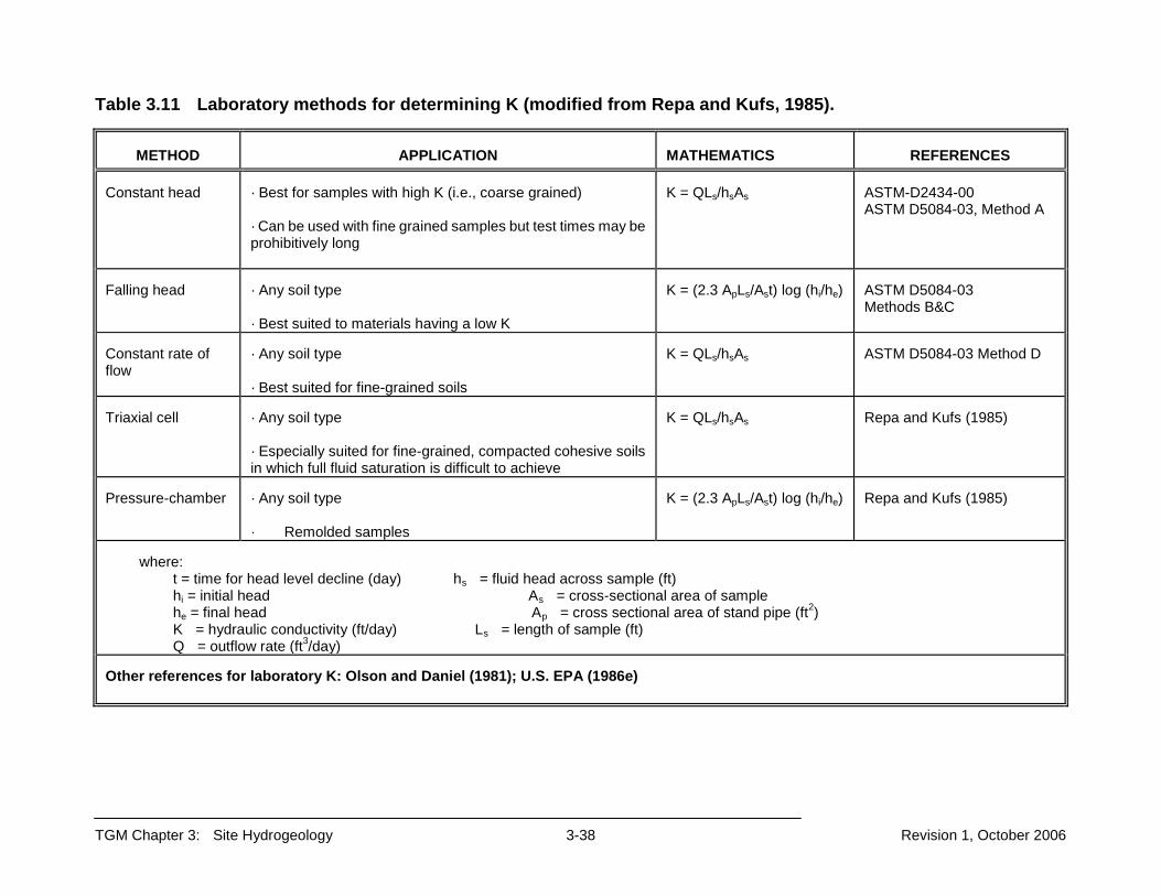
TGM Chapter 3: Site Hydrogeology 3-38 Revision 1, October 2006
Table 3.11 Laboratory methods for determining K (modified from Repa and Kufs, 1985).
METHOD
APPLICATION
MATHEMATICS
REFERENCES
Constant head
· Best for samples with high K (i.e., coarse grained) · Can be used with fine grained samples but test times may be prohibitively long
K = QLs/hsAs
ASTM-D2434-00 ASTM D5084-03, Method A
Falling head
· Any soil type · Best suited to materials having a low K
K = (2.3 ApLs/Ast) log (hi/he)
ASTM D5084-03 Methods B&C
Constant rate of flow
· Any soil type · Best suited for fine-grained soils
K = QLs/hsAs
ASTM D5084-03 Method D
Triaxial cell
· Any soil type · Especially suited for fine-grained, compacted cohesive soils in which full fluid saturation is difficult to achieve
K = QLs/hsAs
Repa and Kufs (1985)
Pressure-chamber
· Any soil type · Remolded samples
K = (2.3 ApLs/Ast) log (hi/he)
Repa and Kufs (1985)
where:
t = time for head level decline (day) hs = fluid head across sample (ft) hi = initial head As = cross-sectional area of sample he = final head Ap = cross sectional area of stand pipe (ft2) K = hydraulic conductivity (ft/day) Ls = length of sample (ft) Q = outflow rate (ft3/day)
Other references for laboratory K: Olson and Daniel (1981); U.S. EPA (1986e)
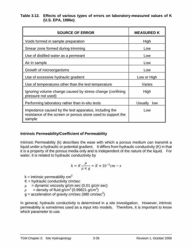
TGM Chapter 3: Site Hydrogeology 3-39 Revision 1, October 2006
Table 3.12. Effects of various types of errors on laboratory-measured values of K (U.S. EPA, 1986e).
SOURCE OF ERROR
MEASURED K Voids formed in sample preparation
High
Smear zone formed during trimming
Low
Use of distilled water as a permeant
Low
Air in sample
Low
Growth of microorganisms
Low
Use of excessive hydraulic gradient
Low or High
Use of temperatures other than the test temperature
Varies
Ignoring volume change caused by stress change (confining pressure not used)
High
Performing laboratory rather than in-situ tests
Usually low
Impedance caused by the test apparatus, including the resistance of the screen or porous stone used to support the sample
Low
Intrinsic Permeability/Coefficient of Permeability
Intrinsic Permeability (k) describes the ease with which a porous medium can transmit a liquid under a hydraulic or potential gradient. It differs from hydraulic conductivity (K) in that it is a property of the porous media only and is independent of the nature of the liquid. For water, it is related to hydraulic conductivity by
k = intrinsic permeability cm2 K = hydraulic conductivity cm/sec μ = dynamic viscosity g/cm-sec (0.01 g/cm sec) ρ = density of fluid g/cm3 (0.99821 g/cm3) g = acceleration of gravity cm/sec (980 cm/sec2)
In general, hydraulic conductivity is determined in a site investigation. However, intrinsic permeability is sometimes used as a input into models. Therefore, it is important to know which parameter to use.

TGM Chapter 3: Site Hydrogeology 3-40 Revision 1, October 2006
Transmissivity Transmissivity is the amount of water that can be transmitted horizontally by the full saturated thickness of a zone. For confined zones, transmissivity is equal to the product of the thickness of the zone (b) and its K:
T = K (b) This equation applies to unconfined units if b is considered to be the saturated thickness or the height of the water table above the top of an underlying confining unit. Field methods for calculating K often involve determining T and then calculating a value with the above equation. Storage Coefficient, Specific Storage, And Specific Yield Storage coefficient (also called storativity) is a dimensionless number that represents the water that a formation releases or absorbs from storage per unit surface area per unit change in head. The storativity of a confined zone is defined as that volume of water released from (or added to) a vertical column of formation of unit horizontal cross-section per unit of decline (or rise) in the piezometric head (Bear, 1972). The storativity of a confined unit is caused by the compressibility of the water and mineral framework and is the product of the specific storage and the thickness. Specific storage is defined by Fetter (2001) as the amount of water per unit volume of a saturated formation that is stored or expelled from storage owing to the compressibility of the mineral skeleton and the pore water per unit change in head. Specific storage has the dimensions of 1/length and generally 0.0001 foot -1 or less. Storativity for confined aquifers generally is on the order of 0.005 or less. Storativity of an unconfined unit is essentially the same except that the decline is in the water table surface; however, the mechanisms causing the variation in the quantity of water stored in a column are different. With unconfined zones, water is drained out of pore space, and air is substituted as the water table drops. The water that is drained by gravity is often referred to as specific yield and the water retained against gravity is called specific retention (Bear, 1972). The specific yield of most alluvial saturated zones falls between 10 and 25% (Bear, 1972). Storativity and specific yield can be determined by pumping tests, which are described in Chapter 4. Flow Rate For investigations of existing or potential pollution sources, it is typically necessary to determine ground water flow rate. Flow rate can be calculated from the hydraulic parameters discussed in the previous section or can be measured by tracer tests. Additional information on tracer tests can be found on page 3-09. Calculation from Hydraulic Parameters In general, ground water flow rate can be determined mathematically based on site-specific parameters. The following equation, derived from Darcy's law, generally is utilized:
V =
Kdh
dl
ne
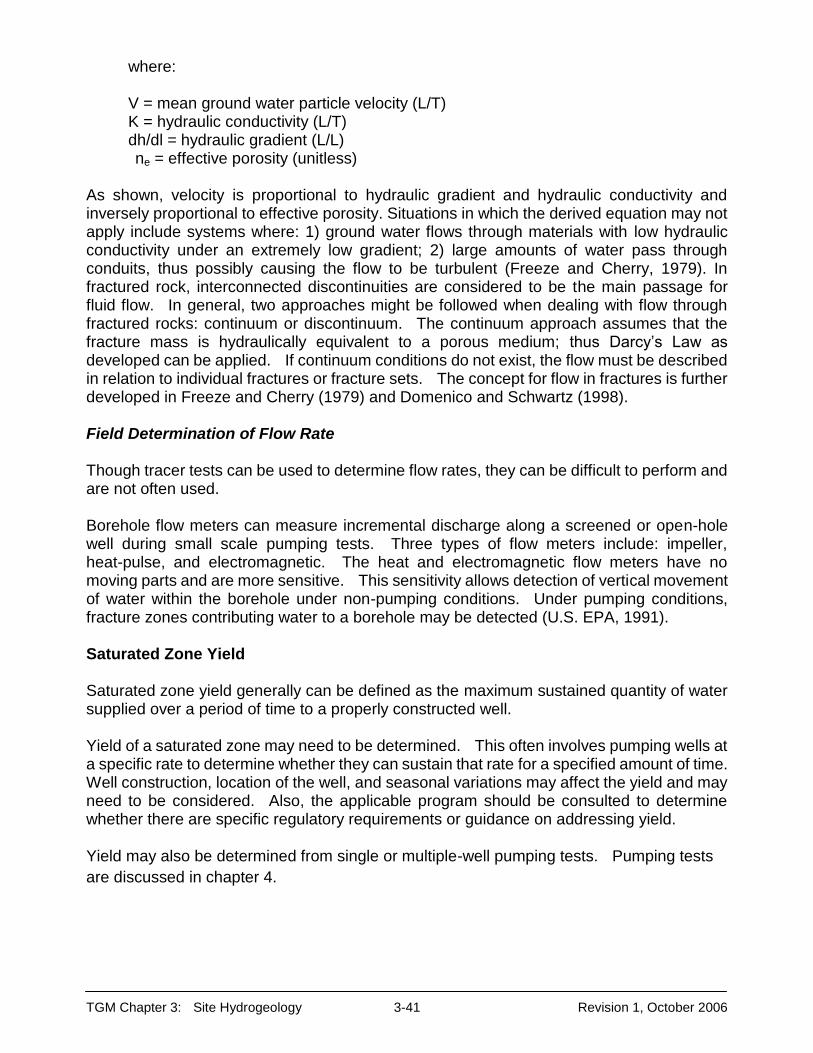
TGM Chapter 3: Site Hydrogeology 3-41 Revision 1, October 2006
where:
V = mean ground water particle velocity (L/T) K = hydraulic conductivity (L/T) dh/dl = hydraulic gradient (L/L) ne = effective porosity (unitless)
As shown, velocity is proportional to hydraulic gradient and hydraulic conductivity and inversely proportional to effective porosity. Situations in which the derived equation may not apply include systems where: 1) ground water flows through materials with low hydraulic conductivity under an extremely low gradient; 2) large amounts of water pass through conduits, thus possibly causing the flow to be turbulent (Freeze and Cherry, 1979). In fractured rock, interconnected discontinuities are considered to be the main passage for fluid flow. In general, two approaches might be followed when dealing with flow through fractured rocks: continuum or discontinuum. The continuum approach assumes that the fracture mass is hydraulically equivalent to a porous medium; thus Darcy’s Law as developed can be applied. If continuum conditions do not exist, the flow must be described in relation to individual fractures or fracture sets. The concept for flow in fractures is further developed in Freeze and Cherry (1979) and Domenico and Schwartz (1998). Field Determination of Flow Rate Though tracer tests can be used to determine flow rates, they can be difficult to perform and are not often used. Borehole flow meters can measure incremental discharge along a screened or open-hole well during small scale pumping tests. Three types of flow meters include: impeller, heat-pulse, and electromagnetic. The heat and electromagnetic flow meters have no moving parts and are more sensitive. This sensitivity allows detection of vertical movement of water within the borehole under non-pumping conditions. Under pumping conditions, fracture zones contributing water to a borehole may be detected (U.S. EPA, 1991). Saturated Zone Yield Saturated zone yield generally can be defined as the maximum sustained quantity of water supplied over a period of time to a properly constructed well. Yield of a saturated zone may need to be determined. This often involves pumping wells at a specific rate to determine whether they can sustain that rate for a specified amount of time. Well construction, location of the well, and seasonal variations may affect the yield and may need to be considered. Also, the applicable program should be consulted to determine whether there are specific regulatory requirements or guidance on addressing yield. Yield may also be determined from single or multiple-well pumping tests. Pumping tests are discussed in chapter 4.

TGM Chapter 3: Site Hydrogeology 3-42 Revision 1, October 2006
GROUND WATER USE DETERMINATION
It is often necessary to determine the ground water use in the vicinity of the area being investigated. PUBLICLY AVAILABLE RECORDS An evaluation of records on file at Ohio EPA, Ohio Department of Natural Resources (ODNR), Department of Agriculture and the local Health Department can assist in determining past, current, or potential ground water use.
· Ohio EPA, Division of Drinking and Ground Waters, regulates public water supplies. Information can be obtained from the district offices on location and discharge rates of public water supplies. In addition, information about drinking water source protection areas for a public water system using ground water can be obtained.
· ODNR, Division of Water, are charged with collecting and maintaining well logs. The
evaluation should include not only those logs for which the well locations have been mapped by ODNR on a U.S.G.S quadrangle, but also those well logs that are on file but have not been mapped by ODNR (herein referred to as unlocated logs). The physical location of the wells should be determined for the unlocated logs. The city and street address and/or driller’s location description can be used to help locate the well and determine if ground water has been used or potentially will be used in the vicinity of the area being investigated.
· A review of county or other local health department records to determine whether well
permits have been issued.
· An inquiry of other local authorities with jurisdiction over installation of wells.
· Each quarry must file an annual water withdrawal report with the ODNR Division of Water, which can provide an estimate of ground water pumpage from the site.
SURVEYS Surveys for wells may also be useful in assessing ground water use. A survey may be as simple as a drive-by observation or as extensive as conducting a door-to-door or mail survey. Interviews or surveys of local drillers to determine whether they have installed wells and/or local water suppliers may help to determine the ground water use in the area. The “level of effort” needed for the survey is site-specific and dependent on the other documentation supporting the well location evaluation. OTHER LINES OF EVIDENCE Other lines of evidence include:
· An ordinance requiring residents/businesses to connect to the public drinking water system.
· A ban on drilling water wells in the area.

TGM Chapter 3: Site Hydrogeology 3-43 Revision 1, October 2006
· A local requirement or ordinance requiring a permit for the installation of a water
supply well.
The weight of the above evidence is dependent on whether these can be, and have been effectively monitored and enforced by the local authority having the jurisdiction.
ANALYSIS AND PRESENTATION OF HYDROGEOLOGIC INFORMATION The data and information collected should be reviewed to determine whether the data quality objectives/requirements were met. This review should not only include data currently collected, but also include all field and laboratory data from previous investigations. Interpretation of field- and laboratory-measured environmental parameters should include a discussion of possible limitations of the method used. Basic assumptions for analytical techniques and methods should be evaluated to determine if site conditions meet assumptions. For example, the analysis of pumping test results should identify the approximate volume of the zone measured by the test and the underlying analytical or other equations used to compute aquifer parameters. If site conditions do not satisfy the assumptions of the solution method, the effect on accuracy and interpretation of results should be stated (ASTM D573-04). Ground water models to simulate flow and contaminant transport may be used to help define the site conditions. Ground water models represent or approximate a real system and are tools that help in the organization and understanding of hydrogeologic data or the prediction of future hydrogeologic events. Models are not a substitute for field investigations, but should be used as supplementary tools. Results are dependent on the quality and quantity of the field data available to define input parameters and boundary conditions (Wang and Anderson, 1982). Results should always be evaluated in context with the fundamental assumptions of the model and the adequacy of the input data. Additional information on the use of models can be found in Chapter 14. To demonstrate that a site has been adequately characterized and proper procedures have been utilized, the data, methodologies, and interpretations should be presented in a report. Components of the report should include, but should not be limited to, a written description, raw data, maps, cross sections, and methodology. Any applicable regulations/rules should be consulted to determine if specific content and format are required. WRITTEN DESCRIPTION A narrative description of the geology and nature and occurrence of ground water should include, at a minimum:
· An evaluation of regional hydrogeology that includes depth to bedrock, characteristics of the major stratigraphic units, average yield of water wells within a one mile radius (logs for wells within one mile also should be submitted10), approximate direction of
10The radial distance may be specified by program requirements. For example, some CERCLA projects may need a 4 mile radius.

TGM Chapter 3: Site Hydrogeology 3-44 Revision 1, October 2006
ground water flow, identification and estimation of the amount of recharge and discharge, geomorphology, and structural geology.
· An accurate classification and description of the consolidated and unconsolidated
materials at the site from the ground surface down to the base of the lowest saturated zone of concern. This may include:
- Hydraulic conductivity (vertical and horizontal).
- Rock and soil types.
- Thickness and lateral extent of units.
- Porosity/effective porosity and bulk density.
- Moisture content.
- The attenuation capacity and mechanism of natural earth materials (such as ion exchange capacity, organic carbon content, mineral content, soil sorptive capacity, storage capacity, pH).
· A site-specific description of structural geology and geomorphology.
· A site-specific description of the occurrence of ground water at the site, including:
- Identification of saturated zones, including depth and lateral and vertical extent. - Identification of zones of high K that may act as preferential pathways. - Identification of zones of low K that may act as barriers to contaminants. - Ground water flow direction and rates (including sample calculations). - Effects of stratification on saturated and unsaturated flow. - Description of the interconnection between saturated zones and surface water. - Description of recharge and discharge areas. -Fluctuations in ground water levels and their effects on flow direction.
· Description of the relationship of the proposed/existing waste management unit to ground
water occurrence and site geology. RAW DATA All raw data collected during the hydrogeologic investigation should be included in the report. This should include, but not be limited to:
· Boring/Geologic Logs: Logs should be provided for all borings. They should be complete technical records of conditions encountered and should include results of laboratory analyses, field identifications, descriptive text, and graphics. Depths/heights should be recorded in fractions (tenths). Logs should be uniform and legible for potential reproduction and submission and should contain, at a minimum, the following information:
- Site name and site-specific coordinates.

TGM Chapter 3: Site Hydrogeology 3-45 Revision 1, October 2006
- The name of the responsible party, the driller, and the on-site geologist. - Method of drilling. - Boring identification number and coordinates. - Date started, date completed, and date abandoned or converted into a well. - Depth of boring. - Surface elevation based on Mean Sea Level (MSL) or fixed referenced. - Method and location of all in-situ sampling. - Condition of samples, percent recovery, blow counts, moisture content, etc. - Materials classification, both field and laboratory. - Depth to water, water-bearing zones and laboratory permeability results. - Color and/or stains. - Presence of structural features, such as fractures, solution cavities, or bedding. - Drilling observations, such as loss of circulation, rig chatter, and heaving sands.
· Well Construction Logs: Construction logs should be provided for all wells
and piezometers used to obtain water level measurements and ground water samples. Information that should be included is listed in Chapter 7. Logs for all wells installed must be submitted to the ODNR, Division of Water (Ohio Revised Code (ORC) 1521.05). Driller contractors may register with ODNR to file water well and drilling reports on-line
(http://www.dnr.state.oh.us/tabid/3252/Default.aspx.)
· Ground Water Elevation Measurements: All ground water elevations should
be submitted in tabulated form. ASTM D6000 method describes basic tabular and graphic methods of presenting data.
· Field Test Data: Raw data from in-situ hydraulic tests should be submitted with
a report. General information that should be submitted is provided in Chapter 4. CROSS SECTIONS An adequate number of cross-sections should be provided. Various orientations (e.g., in direction of ground water flow and orthogonal to ground water flow) should be used. Each cross-section should depict, at a minimum:
· Depth, thickness, classification, and hydraulic characteristics of each unit. · Water table and/or potentiometric surface. · Structures such as zones of fracturing that influence water movement. · Zones of higher K that may influence ground water flow. · Zones of lower K that may restrict and/or attenuate ground water flow. · Location and depth of each boring and/or monitoring well screen. · Orientation of cross-section and horizontal and vertical scales. · Location of proposed or existing waste management areas. · Legend.
MAPS All maps should be legible, have an accurate scale, north arrow, and a legend that contains symbols used on the map. All appropriate locations mentioned in the text should be clearly

TGM Chapter 3: Site Hydrogeology 3-46 Revision 1, October 2006
labeled. Information in the map should be in agreement with data discussed in the text, tables, or in other illustrations. The following maps may assist in demonstrating site hydrogeology:
· A surface topography map depicting (at a minimum) streams, wetlands, depressions, and springs. The map should be constructed by a qualified professional and should provide contour intervals at a level of detail appropriate for the investigation (e.g., two-foot intervals). The map should depict the location of all borings, monitoring wells, and cross-sections. Employment of a conventional or photogrammetric survey company that develops topographic maps by obtaining aerial data often is necessary. Aerial data can be supplemented by data obtained from stereoscopic maps, wetland inventory maps, U.S.G.S. topographic maps, etc.
· A detailed facility map depicting anthropogenic features, including property lines
(with owners of adjacent properties clearly marked), location of all potential contaminant disposal areas, buildings, and utility lines.
· Ground water elevation contour maps for each zone of concern, with actual
measurements at each well/piezometer. Contour lines within the area represented by the data should be represented with a solid line. Any interpretation outside the area should be represented with a dotted or dashed line. An explanation of flow direction and a justification of the extrapolation of flow outside the area defined by the data points should be included in the narrative portion of the report. Flow direction and date water level measurements obtained also should be depicted.
METHODOLOGY The methodology used to evaluate site hydrogeology should be described. This includes, but may not be limited to:
· Number, location, and depth of borings and monitoring wells or piezometers. · Well and piezometer construction and development. · Characterization of soil and rock samples. · Definition of saturated zones and potential confining units. · Rationale for use of indirect methods such as geophysics.

TGM Chapter 3: Site Hydrogeology 3-47 Revision 1, October 2006
REFERENCES Alley, W.M. (editor). 1993. Regional Ground-Water Quality, Van Nostrand Reinhold, New
York, New York. Alyamani, M.S. and Sen, Z. 1993. Determination of Hydraulic Conductivity From Complete
Grain Size Distribution Curves. Ground Water. Vol. 31, No. 4, pp. 551-555. American Society for Testing Materials (ASTM), Method D422-63 (2002)e1. Standard
Methods for Particle-Size Analysis of Soils. American Society of Testing Materials Standards West Conshohocken, Pennsylvania.
ASTM, Method D427-04. Standard Test Method For Shrinkage Factor of Soils. American
Society For Testing Materials Standards.West Conshohocken, Pennsylvania. ASTM, Method D854-06. Standard Methods For Specific Gravity of Soils. American
Society of Testing Material Standards. West Conshohocken, Pennsylvania. ASTM, Method 1556-00. Standard Method for Density of Soils in Place by Sand Cone
Method. American Society of Testing Materials Standards. West Conshohocken, Pennsylvania.
ASTM, Method 1557-02e1. Standard Methods for Moisture-Density Relationships of Soils
and Soil Aggregating Mixtures Using 10 lb. (4.54 Kg) Hammer and 18 in. (457-mm) Drop. American Society of Testing Materials Standards. Philadelphia, Pennsylvania. Vol. 04.08, pp. 118-125.West Conshohocken, Pennsylvania.
ASTM, Method D2167-94 (2001). Standard Method for Density and Unit Weight of Soil in
Place by Rubber Balloon Method. American Society of Testing Materials Standards (reapproved 1990). West Conshohocken, Pennsylvania.
ASTM, Method D2216-05. Standard Method For Laboratory Determination of Water
(Moisture) Content of Soils, Rock, and Soil-Aggregate. American Society of Testing Materials Standards. West Conshohocken, Pennsylvania.
ASTM, Method D2434-00e1. Standard Method for Permeability of Granular Soils (Constant
Head). American Society of Testing Materials Standards. West Conshohocken, Pennsylvania.
ASTM, Method D2487-06. Standard Method For Classification of Soils for Engineering
Purposes. American Society of Testing Materials Standards. West Conshohocken, Pennsylvania.
ASTM, Method D2488-00. Standard Method For Description and Identification of Soils
(Visual Manual Procedure). Annual Book of American Society of Testing Materials Standards. West Conshohocken, Pennsylvania.

TGM Chapter 3: Site Hydrogeology 3-48 Revision 1, October 2006
ASTM, Method D2937-04. Standard Method For Density of Soil in Place by Drive Cylinder Method. American Society of Testing Materials Standards (reapproved 1990). West Conshohocken, Pennsylvania.
ASTM, Method D3017-05. Standard Method For Moisture Content of Soil and
Soil-Aggregate in Place by Nuclear Method (Shallow Depth). American Society of Testing Materials Standards. West Conshohocken, Pennsylvania.
ASTM, Method D3385-03. Standard Method For Infiltration Rate of Soils in Field Using
Double-Ring Infiltrometers. American Society of Testing Materials Standards. West Conshohocken, Pennsylvania.
ASTM, Method D3441-05 Standard Method For Deep Quasi-state, Cone and Friction-cone
Penetration Tests of Soils. American Society of Testing Material Standards. West Conshohocken, Pennsylvania.
ASTM, Method D4318-05. Standard Test Method for Liquid Limit, Plastic Limit, and
Plasticity Index for Soils. American Society of Testing Materials Standards. West Conshohocken, Pennsylvania.
ASTM, Method 4943-02. Standard Method for Shrinking Factors of Soils by Wax Method.
American Society of Testing Materials Standards.West Conshohocken, Pennsylvania. ASTM, Method D4959-00. Standard Method for Determination of Water (Moisture)
Content of Soils by Direct Heating Methods. American Society of Testing Materials Standards.West Conshohocken, Pennsylvania.
ASTM, Method D4972-01 Standard Tests Method for pH in Soils. American Society of
Testing Materials Standards. West Conshohocken, Pennsylvania. ASTM, Method D5084-03 Standard Method For Measurement of Hydraulic Conductivity
of Saturated Porous Materials Using a Flexible Wall Permeameter. American Society of Testing Materials. West Conshohocken, Pennsylvania.
ASTM, Method D5093-02 Standard Method For Field Measurement of Infiltration Using a
Double Ring Infiltrometer With a Sealed Inner Ring. American Society of Testing Materials. West Conshohocken, Pennsylvania.
ASTM, Method D5778-95 (2000). Standard Test Method for Performing Electronic Friction
Cone and Piezocone Penetration Testing of Soils American Society of Testing Materials. West Conshohocken, Pennsylvania.
ASTM, Method D6000-98 (2002). Standard Method for Presentation of Water-Level
Information From Ground-Water Sites. American Society of Testing Materials. West Conshohocken, Pennsylvania.

TGM Chapter 3: Site Hydrogeology 3-49 Revision 1, October 2006
Baehr, T. R., and W. L. Turley, 2000, Seasonal and Temporal Water Level Trends in Glacial Till Deposits (Abstract): in A Conference on Fractured Glacial Tills, R. J. Haefner, Ed., Water Management Association of Ohio Spring Conference, May 9-10, 2000, Columbus, Ohio, p. 22.
Barari, A., and L. S. Hedges, 1985, Movement of Water in Glacial Till: in Proceedings of the
17th International Congress, International Association of Hydrogeologists, Hydrogeology of Rocks of Low Permeability, International Association of Hydrogeologists, pp. 129-136.
Bear, J. 1988. Dynamics of Fluids in Porous Media.,Dover Publications. New York. Benson, R. C.2006. Second Edition. Remote Sensing and Geophysical Methods for
Evaluation of Subsurface Conditions. In: D. M. Nielsen (editor), Practical Handbook of Environmental Site Characterization Ground-Water Monitoring.Taylor & Francis. Boca Raton, Florida. pp. 249-295.
Black, C. A. (editor). 1965a. Methods of Soil Analysis. Part 1. Physical and Mineralogical
Properties, Including Statistics of Measuring Samples. Society of Agronomy Inc. Madison, Wisconsin.
Black, C. A. (editor). 1965b. Methods of Soil Analysis. Part 2. Chemical and Microbiological
Properties. American Society of Agronomy. Madison, Wisconsin. Bradbury, K. R., Desaulniers, D. S., Connell, D. E., and R. G. Hennings, 1985, Groundwater
Movement Through Clayey Till, Northern Wisconsin, USA: in Proceedings of the 17th International Congress, International Association of Hydrogeologists, Hydrogeology of Rocks of Low Permeability, International Association of Hydrogeologists, pp. 405-416.
Bruner, D. R., and A. J. Lutenegger, 1993, Measurement of Saturated Hydraulic
Conductivity in Fine-Grained Glacial Tills in Iowa: Comparison of In Situ and Laboratory Methods: in Hydraulic Conductivity and Waste Contaminant Transport in Soils, ASTM STP 1142, D. E. Daniel and S. J. Trautwein, Eds., American Society for Testing and Materials, Philadelphia.
Bouwer, H. 1978. Groundwater Hydrology. McGraw-Hill Book Company. New York. Cravens, S. J., and L. C. Ruedisili, Water Movement in Till of East-Central South Dakota:
Ground Water, Vol. 25, No. 5 pp. 555-561. Cook, P. and A.L. Herzeg (editors). 2000. Environmental Tracers in Subsurface
Hydrogeology. Kluwer Academic Publishers. Boston, Massachusetts. Compton, R.R. 1985. Geology in the Field. John Wiley and Son. New York.

TGM Chapter 3: Site Hydrogeology 3-50 Revision 1, October 2006
Dalton, M. G., B. E. Huntsman, and K. Bradbury. 2006. Acquisition and Interpretation of Water-Level Data. In: D. M. Nielsen (editor), Practical Handbook of Environmental Site Characterization and Ground-Water Monitoring. Taylor & Francis. Boca Raton, Fl. pp. 883-911.
Davis, S. N., D. J. Campbell, H. W. Bently, and T. J. Flynn. 1985. Ground Water Tracers.
Cooperative Agreement CR-80036, U.S. Environmental Protection Agency. National Ground Water Association, Dublin, OH.
D’Astous, A. Y., Ruland, W. W., Bruce, J. R. G., Cherry, J. A., and R. W. Gillham, 1989,
Fracture Effects in the Shallow Groundwater Zone in Weathered Sarnia-Area Clay: Can. Geotech. J., Vol 26., pp. 43-56.
Dawson, K. and J. D. Istok. 1991. Aquifer Testing, Design and Analysis of Pumping and
Slug Tests. Lewis Publishers, Inc. Chelsea, Michigan. Döll, P., and W. Schneider, 1995, Lab and Field Measurements of the Hydraulic
Conductivity of Clayey Silts: Ground Water, Vol. 33, No. 6, pp. 884-891. Domenico, P.A. and F.W. Schwartz. 1997. Second Edition. Physical and Chemical
Hydrogeology. John Wiley and Sons. New York. Fair, G. M., and L. P. Hatch. 1933. Fundamental Factors Governing the Streamline Flow of
Water Through Sand. Journal of American Water Works Association. Vol. 25, No. 11, pp. 1551-1561.
Fetter, C. W. 2001. Applied Hydrogeology. Fourth Edition. Prentice Hall. Uper
Saddle River, New Jersey. Freeze, R. A. and J. A. Cherry. 1979. Groundwater. Prentice-Hall Inc. Englewood Cliffs,
New Jersey. Gerber, R. E., and K. Howard, 2000, Recharge Through a Regional Till Aquitard:
Three-Dimensional Flow Model Water Balance Approach: Ground Water, Vol. 38, No. 3, pp. 410-422.
Golder Associates, Inc. 1990. Final Report on Breakthrough and Leachate Compatibility
Testing of Typical Clay Liner Materials, Adams Center Facility, Fort Wayne, Indiana. Prepared for Chemical Waste Management of Indiana, Inc.
Hazen, A. 1911. Discussion of "Dams on Sand Foundation" by A. C. Koenig. Transactions
American Society of Civil Engineers. Vol. 73, pp. 199-203. Heath, R. C. 1984. Basic Ground-Water Hydrology. U.S. Geological Survey
Water-Supply Paper 2200. United States Government Printing Office. Alexandria, Virginia.

TGM Chapter 3: Site Hydrogeology 3-51 Revision 1, October 2006
Hendry, M. J., 1988, Hydraulic Conductivity of a Clay Till in a Prairie Region of Canada: Ground Water, Vol. 26, No. 5, pp. 607-614
Hendry, M. J., 1982, Hydraulic Conductivity of a Glacial Till in Alberta: Ground Water, Vol.
20, No. 2, pp. 162-169. Hendry, M. J., Cherry, J. A., and E. I. Wallick, 1986, Origin and Distribution of Sulfate in a
Fractured Till in Southern Alberta, Canada: Water Resources Research, Vol. 22, No. 1, pp. 45-61
Holtz, R. D. and W. D. Kovacs, 1981. An Introduction to Geotechnical Engineering.
Prentice-Hall. Englewood Cliffs, New Jersey. Javandel, I. 1984. Methods of Evaluating Vertical Ground Water Movement. Earth
Science Division. Lawrence Berkeley Laboratory. University of California, Berkeley, California.
Jones, L., 1993, A Comparison of Pumping and Slug Tests for Estimating the Hydraulic
Conductivity of Unweathered Wisconsian Age Till in Iowa: Ground Water, Vol. 31, No. 6, pp. 896-904.
Jury, W. A. 1986. Adsorption of Organic Chemicals Onto the Soil. In: S. C. Hern and S.
M. Melancon (editors), Vadose Zone Modeling of Organic Pollutants. Lewis Publishers Inc. Chelsea, Michigan. pp. 177-190.
Keller, C. K., van der Kamp, G., Cherry, J. A., 1991, Hydrogeochemistry of a Clayey Till - 1.
Spatial Variability: Water Resources Research, Vol. 27, No. 10, pp. 2543-2554. Keller, C. K., van der Kamp, G., Cherry, J. A., 1989, A Multiscale Study of the Permeability of
a Thick Clayey Till: Water Resources Research, Vol. 25, No. 11, pp. 2299-2317. Keller, C. K., van der Kamp, G., Cherry, J. A., 1988, Hydrogeology of Two Saskatchewan
Tills, I. Fractures, Bulk Permeability, and Spatial Variability of Downward Flow: Journal of Hydrology, Vol. 101, pp. 97-121.
Keller, C. K., van der Kamp, G., Cherry, J. A., 1986, Fracture Permeability and Groundwater
Flow in Clayey Till near Saskatoon, Saskatchewan: Can. Geotech J., Vol. 23, pp. 229-240.
Kerfoot, W. B. 1988. Monitoring Well Construction and Recommended Procedures for
Direct Ground-Water Flow Measurements Using a Heat-Pulsing Flowmeter. In: A. G. Collins and A. I. Johnson (editors), Ground-water Contamination: Field Methods. ASTM Special Technical Publication 963. Philadelphia, Pennsylvania. pp. 146-161.
Keys, W.S. and L.M. MacCary. 1971. Techniques of Water Resource Investigation of the Unites States Geological Survey, Chapter E1: Application of Borehole Geophysics to

TGM Chapter 3: Site Hydrogeology 3-52 Revision 1, October 2006
Ground Water Investigations. U.S. Geological Survey. Book 2: Collection of Environmental Data. U.S. Government Printing Office. Washington D.C.

TGM Chapter 3: Site Hydrogeology 3-53 Revision 1, October 2006
Kinner, N.E., R.W. Masters, and L.B. Fournier. 2005. Fractured Rock: State of the Science and Measuring Success in Remediation. National Ground Water Association. Source: http://clu-in.org/fracrock.
Kulander, B.R., C.C. Barton, and S.L. Dean. 1990. Fracture Core Analysis:
Interpretation, Logging, and Natural and Induced Fractures in Core. American Association of Petroleum Geologists. Methods in Exploration Series, No. 8. Tulsa, Oklahoma.
McKay, L.D.; D.J. Balfour, J.A. Cherry. 1998. Lateral Chloride Migration from a Landfill in
Fracture Clay Rich Glacial Deposit. Ground Water. Volume 36, No. 6, pp. 988-999. Morrison, R. D. 1983. Ground Water Monitoring Technology. TIMCO MFC. Inc.
Publication. Prairie Du Sac, Wisconsin. Nielsen, D., G.L. Nielsen, and L.M. Preslo. 2006 (Second Edition). Environmental Site
Characterization. In: D. M. Nielsen (editor), Practical Handbook of Environmental Site Characterization Ground-Water Monitoring.Taylor & Francis. Boca Raton, Florida. pp. 35-2005.
Olson, R. E. and D. F. Daniel. 1981. Measurement of Hydraulic Conductivity of
Fine-Grained Soils. In: T.F. Zimmie and C. O. Riggs (editors), Permeability and Groundwater Contaminant Transport. ASTM Special Publication 746. Philadelphia, Pennsylvania. pp. 18-64.
Plummer, L.N. and E. Busenberg. 2000. Chapter 15: Chlorofluorocarbons. In P. Cook
and A.L. Herczeg (editors): Environmental Tracers in Subsurface Hydrology. Kluwer Academic Publishers. Boston, Massachusetts.
Prudic, D. E., Hydraulic Conductivity of a Fine-Grained Till, Cattaraugus County, New York,
1982: Ground Water, Vol. 20, No. 2, pp. 194-204. Rawls, W. J., D. L. Brakensiek, and N. Miller. 1983. Green-Ampt Infiltration Parameters
from Soils Data. ASCE Journal of Hydraulic Engineering. Vol. 9, No. 102. Repa, E. and C. Kufs. 1985. Leachate Plume Management. Hazardous Waste
Engineering Research Laboratory. Office of Solid Waste and Emergency Response. U.S. Environmental Protection Agency. EPA/540/2-85/004.
Robertson, P. K. and R. G. Campanella. 1986. Guidelines For Use and Interpretation of
Electric Cone Penetration Tests. Third Edition. Hogentogler and Company. Gaithersburg, Maryland.
Ruda, T. and J. Farrar. 2006. Environmental Drilling for Soil Sampling, Rock Coring,
Monitoring Well Drilling, Borehole Logging and Monitoring Well Installation. In: D. M. Nielsen (editor), Practical Handbook of Environmental Site Characterization Ground-Water Monitoring. Taylor & Francis Group, LLC. Boca Raton, Florida. pp. 297-344.

TGM Chapter 3: Site Hydrogeology 3-54 Revision 1, October 2006
Rudolph, D. L., Cherry, J. A., and R. N. Farvolden, 1991, Groundwater Flow and Solute Transport in Fractured Lacustrine Clay Near Mexico City: Water Resources Research, Vol. 27, No. 9, pp. 2187-2201.
Ruland, W. W., Cherry, J. A., and S. Feenstra, 1991, The Depth of Fractures and Active
Ground-Water Flow in a Clayey Till Plain in Southwestern Ontario: Ground Water, Vol. 29, No. 3, pp. 405-417
Sara, M.C. 2003. Site Assessment and Remediation Handbook. Second Edition. CRC
Press, Lewis Publications. pp. Sevee, J. 2006. Second Edition. Methods and Procedures for Defining Aquifer
Parameters. In: D. M. Nielsen (editor), Practical Handbook of Environmental Site Characterization Ground-Water Monitoring. Taylor & Francis Group, LLC. Boca Raton, Florida. pp. 913-958.
Simpkins, W. W., and K. R. Bradbury, 1992: Journal of Hydrology, Vol. 132, pp. 283-319. Smolley, M. and J. C. Kappmeyer. 1991. Cone Penetrometer Tests and Hydropunch
Sampling: A Screening Technique for Plume Definition. Ground Water Monitoring Review. Vol. 11, No. 2, pp. 101-106.
Solomon, D.K. and P.G. Cook. 200. 3H and 3He. In P. Cook and A.L. Herczeg (editors):
Environmental Tracers in Subsurface Hydrology. Kluwer Academic Publishers. Boston, Massachusetts.
Strobel, M. L., 1993, Hydraulic Properties of Three Types of Glacial Deposits In Ohio: U.S.
Geological Survey Water-Resources Investigations Report 92-4135. Todd, D. K. 2004. Ground Water. Third Edition. John Wiley and Sons. New York. U.S. EPA. 1998. Estimation of Infiltration Rate in the Vadose Zone: Compilation of Simple
Mathematical Models. Volume 1. United States Environmental Program, National Risk Management Research Laboratory. EPA/600/R-97/128a. Ada, Ok.
U.S. EPA. 1998. Estimation of Infiltration Rate in the Vadose Zone: Compilation of Simple
Mathematical Models. Volume 11. United States Environmental Program, National Risk Management Research Laboratory. EPA/600/R-97/128b. Ada, Ok.
U.S. EPA. 1997. Expedited Site Assessment Tools for Underground Storage Tanks
Sites. A Guide for Regulators. U.S. Environmental Protection Agency, Solid and Emergency Response. EPA 510-B-97-001.
U.S. EPA. 1992. RCRA Ground-Water Monitoring Draft Technical Guidance. Office of
Solid Waste. U.S. Environmental Protection Agency. Washington, D.C. U.S. EPA.1991. Site Characterization for Subsurface Remediation. Office of Research
and Development. EPA/625/4-91/026.

TGM Chapter 3: Site Hydrogeology 3-55 Revision 1, October 2006
U.S. EPA. 1987. A Compendium of Superfund Field Operations Methods. Vol. 1 and 2.
EPA/540/P- 87/001a and 001b. Office of Emergency and Remedial Response. Washington, D.C.
U.S. EPA. 1986a. Cation-Exchange Capacity of Soils (Ammonium Acetate). In: Test
Methods For Evaluating Solid Waste. SW846, Method 9080. Office of Solid Waste and Emergency Response. Washington, D.C.
U.S. EPA. 1986b. Cation-Exchange Capacity of Soils (Sodium Acetate). In: Test
Methods for Evaluating Solid Waste. SW846, Method 9081. Office of Solid Waste and Emergency Response. Washington, D.C.
U.S. EPA 1986c. Criteria for Identifying Areas of Vulnerable Hydrogeology Under the
Resource Conservation and Recovery Act. [Statutory Interpretive Guidance. Guidance Manual for Hazardous Waste Land Treatment, Storage and Disposal Facilities.] Interim Final. Office of Solid Waste and Emergency Response, Washington, D.C.
U.S. EPA. 1986d. RCRA Ground Water Technical Enforcement Guidance Document.
Office of Waste Program Enforcement, Office of Solid Waste and Emergency Response. OSWER 9950.1. Washington, D.C.
U.S. EPA. 1986e. Saturated Hydraulic Conductivity, Saturated Leachate Conductivity and
Intrinsic Permeability. In: Test Methods For Evaluating Solid Waste. SW846, Method 9100. Office of Solid Waste and Emergency Response. Washington, D.C.
U.S. EPA. 1986f. Soil pH. In: Test Methods for Evaluating Solid Waste. SW846, Method 9045. Office of Solid Waste and Emergency Response. Washington, D.C. U.S. EPA. 1986g. Total Organic Carbon. In: Test Methods For Evaluating Solid
Waste. SW846, Method 9060. Office of Solid Waste and Emergency Response. Washington, D.C.
U.S. EPA. 1991. Ground Water Vol. II. Methodology, Office of Research and
Development. U.S. Environmental Protection Agency. Washington D.C. EPA/626/6-90/061b.
U.S. EPA. 1993. Subsurface Characterization and Monitoring Techniques. A Desk
Reference Guide. Volume II: The Vadose Zone Field, Screening and Analysis Methods. Appendix C & D. EPA/625/R-23/003b.
U.S. G.S. 1993. Current Water Resources Activities in Ohio 1993-1994. Open-File
Report 93-458. U.S. Geological Survey, Earth Science Information Center. Denver, Colorado.

TGM Chapter 3: Site Hydrogeology 3-56 Revision 1, October 2006
CHAPTER 3: APPENDIX I
GEOPHYSICAL METHODS FOR SITE CHARACTERIZATION

TGM Chapter 3: Site Hydrogeology 3-57 Revision 1, October 2006
Table A3.1 Typical applications of surface geophysical methods (Benson et al, 1982). APPLICATION
RADAR
EM
RES
SEISMIC
MD
MAG
NATURAL CONDITIONS Layer thickness and depth of soil and rock Mapping lateral anomaly locations Determining vertical anomaly depths Very high resolution of lateral or vertical anomalous conditions Depth to water table
1 1 1 1 2
2 1 2 1 2
1 1 1 2 1
1 1 1 2 1
N/A N/A N/A N/A N/A
N/A** N/A** N/A N/A N/A
SUB-SURFACE CONTAMINATION LEACHATES/PLUMES Existence of contaminant (Reconnaissance Surveys) Mapping contaminant boundaries Determining vertical extent of contaminant Quantify magnitude of contaminants Determine flow direction Flow rate using two measurements at different times Detection of organics floating on water table Detection & mapping of contaminants within unsaturated zone
2* 2* 2* N/A 2* N/A 2*
2
1 1 2 1 1 1 2* 1
1 1 1 1 1 1 2* 1
N/A N/A N/A N/A N/A N/A N/A N/A
N/A N/A N/A N/A N/A N/A N/A N/A
N/A N/A N/A N/A N/A N/A N/A N/A
LOCATION AND BOUNDARIES OF BURIED WASTES Bulk wastes Non-metallic containers Metallic containers - Ferrous - Non-Ferrous Depth of burial
1 1 2 2 2
1 1 1 1 2
1 1 N/A N/A 1
2 2 N/A N/A 2
N/A N/A 1 1 2*
N/A N/A 1 N/A 2*
UTILITIES Location of pipes, cables, tanks Identification of permeable pathways associated with loose fill in utility trenches Abandoned well casings
1 1 N/A
1 1 N/A
N/A N/A N/A
2 2 N/A
1 1 1
1 1 1
SAFETY Pre-drilling site clearance to avoid drums, breaching trenches, etc.
1
1
2
N/A
1
1
GPR=ground penetrating radar, EM=electromagnetics, RES=resistivity, MD=metal detection, MAG=magnetometric 1 primary use 2 possible applications, secondary use; however, in some special cases this method may be the only effective approach due to circumstances. N/A Not applicable * Limited application ** Not applicable in the context used in this document.

TGM Chapter 3: Site Hydrogeology 3-58 Revision 1, October 2006
Table A3.2 Surface geophysical methods for locating and mapping of buried wastes and utilities (Benson, 2006).a METHOD
BULK WASTES
WITHOUT METALS
BULK WASTES WITH METALS
55 GALLON DRUMS
PIPES AND
TANKS
GPR
Very good if soil conditions are appropriate; sometimes effective to obtain shallow boundaries in poor soil conditions
Very good if soil conditions are appropriate; sometimes effective to obtain shallow boundaries in poor soil conditions
Good if soil conditions are appropriate (may provide depth)
Very good for metal and non-metal if soil conditions are appropriate (may provide depth)
EM
Excellent to depths less than 20 feet
Excellent to depths less than 20 feet
Very good (single drum to 6-8 feet)
Very good for metal tanks
Resistivity
Good (sounding may provide depth)
Good (sounding may provide depth)
-N/A-
-N/A-
Seismic Refraction
Fair (may provide depth)
Fair (may provide depth)
-N/A-
-N/A-
Micro- Gravity
Fair (may provide depth)
Fair (may provide depth)
-N/A-
-N/A-
Metal Detector
-N/A-
Very good (shallow)
Very good (shallow)
Very good (shallow)
Magneto-meter
-N/A-
Very good (ferrous only; deeper than metal detector)
Very good (ferrous only; deeper than metal detector)
Very good (ferrous only; deeper than metal detector)
a Applications and comments should only be used as guidelines. In some applications, an alternate method may provide better results.

TGM Chapter 3: Site Hydrogeology 3-59 Revision 1, October 2006
Table A3.3 Surface geophysical methods for evaluation of natural hydrogeologic conditions (Benson, 2006).a
Method
General
Application
Continuous Measurement
Depth
Application
Major Limitations
GPR
Profiling and mapping; highest resolution of any method
yes
to 100 feet (typically less than 30 feet
Penetration limited by soil type and saturation conditions
EM (Frequency Domain)
Profiling and mapping, very rapid measurements
yes
(50 feet)
to 200 feet
Affected by cultural features (metal fences, pipes, buildings, vehicles)
EM (Time Domain)
Soundings
no
to a few thousand feet
Does not provide measurements shallower than about 150 feet
Resistivity
Soundings or profiling and mapping
no
No limit (commonly used to a few hundred feet)
Requires good ground contact and long electrode arrays. Integrates a large volume of subsurface. Affected by cultural features (metal fences, pipes, buildings, vehicles).
Seismic Refraction
Profiling and mapping
no
No limit (commonly used to a few hundred feet)
Requires considerable energy for deeper surveys. Sensitive to ground vibrations.
Seismic Reflection
Profiling and mapping
no
Can use to a few thousand feet; depths of 50 to 100 feet are common in hydrogeologic studies
Sensitive to ground vibrations. Loose soils near surface limits the method. Very slow, requires extensive data reduction.
Micro Gravity
Profiling and mapping
no
No limit (commonly used to upper 100 feet)
Very slow, requires extensive data reduction. Sensitive to ground vibrations
Magnetics
Profiling and mapping
yes
No limit (commonly used to a few hundred feet)
Only applicable in certain rock environments. Limited by cultural ferrous metal features.
a Applications and comments should be used as guidelines. In some applications, alternative methods may provide better results.
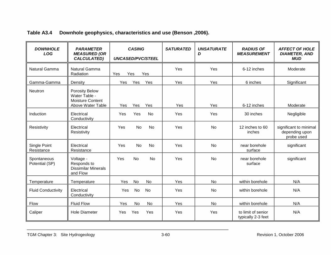
TGM Chapter 3: Site Hydrogeology 3-60 Revision 1, October 2006
Table A3.4 Downhole geophysics, characteristics and use (Benson ,2006). DOWNHOLE LOG
PARAMETER MEASURED (OR CALCULATED)
CASING UNCASED/PVC/STEEL
SATURATED
UNSATURATED
RADIUS OF MEASUREMENT
AFFECT OF HOLE DIAMETER, AND MUD
Natural Gamma
Natural Gamma Radiation
Yes Yes Yes
Yes
Yes
6-12 inches
Moderate
Gamma-Gamma
Density
Yes Yes Yes
Yes
Yes
6 inches
Significant
Neutron
Porosity Below Water Table - Moisture Content Above Water Table
Yes Yes Yes
Yes
Yes
6-12 inches
Moderate
Induction
Electrical Conductivity
Yes Yes No
Yes
Yes
30 inches
Negligible
Resistivity
Electrical Resistivity
Yes No No
Yes
No
12 inches to 60
inches
significant to minimal
depending upon probe used
Single Point Resistance
Electrical Resistance
Yes No No
Yes
No
near borehole
surface
significant
Spontaneous Potential (SP)
Voltage - Responds to Dissimilar Minerals and Flow
Yes No No
Yes
No
near borehole
surface
significant
Temperature
Temperature
Yes No No
Yes
No
within borehole
N/A
Fluid Conductivity
Electrical Conductivity
Yes No No
Yes
No
within borehole
N/A
Flow
Fluid Flow
Yes No No
Yes
No
within borehole
N/A
Caliper
Hole Diameter
Yes Yes Yes
Yes
Yes
to limit of senior typically 2-3 feet
N/A
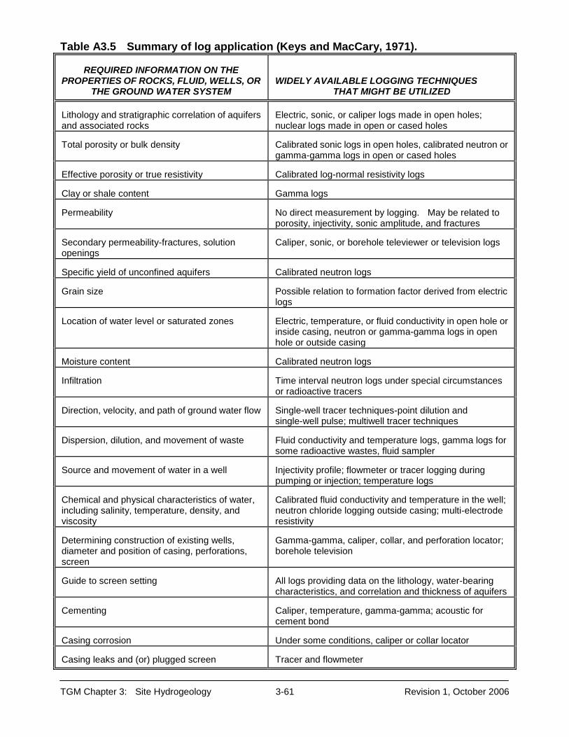
TGM Chapter 3: Site Hydrogeology 3-61 Revision 1, October 2006
Table A3.5 Summary of log application (Keys and MacCary, 1971).
REQUIRED INFORMATION ON THE PROPERTIES OF ROCKS, FLUID, WELLS, OR
THE GROUND WATER SYSTEM
WIDELY AVAILABLE LOGGING TECHNIQUES THAT MIGHT BE UTILIZED
Lithology and stratigraphic correlation of aquifers and associated rocks
Electric, sonic, or caliper logs made in open holes; nuclear logs made in open or cased holes
Total porosity or bulk density
Calibrated sonic logs in open holes, calibrated neutron or gamma-gamma logs in open or cased holes
Effective porosity or true resistivity
Calibrated log-normal resistivity logs
Clay or shale content
Gamma logs
Permeability
No direct measurement by logging. May be related to porosity, injectivity, sonic amplitude, and fractures
Secondary permeability-fractures, solution openings
Caliper, sonic, or borehole televiewer or television logs
Specific yield of unconfined aquifers
Calibrated neutron logs
Grain size
Possible relation to formation factor derived from electric logs
Location of water level or saturated zones
Electric, temperature, or fluid conductivity in open hole or inside casing, neutron or gamma-gamma logs in open hole or outside casing
Moisture content
Calibrated neutron logs
Infiltration
Time interval neutron logs under special circumstances or radioactive tracers
Direction, velocity, and path of ground water flow
Single-well tracer techniques-point dilution and single-well pulse; multiwell tracer techniques
Dispersion, dilution, and movement of waste
Fluid conductivity and temperature logs, gamma logs for some radioactive wastes, fluid sampler
Source and movement of water in a well
Injectivity profile; flowmeter or tracer logging during pumping or injection; temperature logs
Chemical and physical characteristics of water, including salinity, temperature, density, and viscosity
Calibrated fluid conductivity and temperature in the well; neutron chloride logging outside casing; multi-electrode resistivity
Determining construction of existing wells, diameter and position of casing, perforations, screen
Gamma-gamma, caliper, collar, and perforation locator; borehole television
Guide to screen setting
All logs providing data on the lithology, water-bearing characteristics, and correlation and thickness of aquifers
Cementing
Caliper, temperature, gamma-gamma; acoustic for cement bond
Casing corrosion
Under some conditions, caliper or collar locator
Casing leaks and (or) plugged screen
Tracer and flowmeter

TGM Chapter 3: Site Hydrogeology 3-62 Revision 1, October 2006
end of document

State of Ohio Environmental Protection Agency
Division of Drinking and Ground Waters
Technical Guidance Manual for Ground Water Investigations Chapter 4
Pumping and Slug Tests
December 2006 Governor : Ted Strickland Director : Chris Korleski

TECHNICAL GUIDANCE MANUAL FOR
GROUND WATER INVESTIGATIONS
CHAPTER 4
Pumping and Slug Tests
December 2006
Revision 1
Ohio Environmental Protection Agency Division of Drinking and Ground Waters
P.O. Box 1049 50 West Town Street Columbus, Ohio 43216-1049
Phone: 614-644-2752 http://www.epa.state.oh.us/ddagw/

TGM Chapter 4: Pumping and Slug Tests 4-ii Revision 1, December 2006
PREFACE
This chapter contains guidance for conducting and reporting on pumping and slug tests at sites that are being characterized because of suspected or known contamination, or are being evaluated for waste disposal. This chapter does not cover pumping tests for determining whether a ground water zone is capable of producing a sufficient yield for supply purposes. This document is part of a series of chapters incorporated in Ohio EPA’s Technical Guidance Manual for Hydrogeologic Investigations and Ground Water Monitoring (TGM), which was originally published in 1995. DDAGW now maintains this technical guidance as a series of chapters rather than as an individual manual. The chapters can be obtained at http://www.epa.state.oh.us/ddagw/tgmweb.aspx. The TGM identifies technical considerations for performing hydrogeologic investigations and ground water monitoring at potential or known ground water pollution sources. The purpose is to enhance consistency within the Agency and inform the regulated community of the Agency’s technical recommendations and the basis for them. In Ohio, the authority over pollution sources is shared among various Ohio EPA divisions, including the Emergency and Remedial Response (DERR), Hazardous Waste Management (DHWM), Solid and Infectious Waste (DSIWM), and Surface Water (DSW), as well as other state and local agencies. DDAGW provides technical support to these divisions. Ohio EPA utilizes guidance to aid regulators and the regulated community in meeting laws, rules, regulations and policy. Guidance outlines recommended practices and explains their rationale. The Agency may not require an entity to follow methods recommended by this or any other guidance document. It may, however, require an entity to demonstrate that an alternate method produces data and information that meet the pertinent requirements. The procedures used to meet requirements usually should be tailored to the specific needs and circumstances of the individual site, project, and applicable regulatory program, and should not comprise a rigid step-by-step approach that is utilized in all situations.

TGM Chapter 4: Pumping and Slug Tests 4-iii Revision 1, December 2006
Major Changes from the February 1995 TGM The Ohio EPA Technical Guidance Manual for Hydrogeologic Investigations and Ground Water Monitoring (TGM) was finalized in 1995. This guidance document represents an update to Chapter 4 (Pumping and Slug Tests). Listed below are the major changes from the 1995 version. 1. Simplified the tables summarizing the various test analysis methods by removing
detailed information that a reader could only understand if they were familiar with the details of the method.
2. Removed figures. Problems were encountered with obtaining permission to use figures
from sources other than government documents. 3. Updated references. 4. Placed less focus on workplans and more on what and how pump and slug test data
should be submitted.
TGM Chapter 4: Pumping and Slug Tests 4-iv Revision 1, December 2006
TABLE OF CONTENTS PREFACE .................................................................................................................... 4-ii MAJOR CHANGES FROM THE FEBRUARY 1995 TGM ............................................ 4-iii SLUG TESTS ............................................................................................................... 4-1
DESIGN AND PERFORMANCE OF SLUG TEST .................................................. 4-2 Design of Well ................................................................................................... 4-2 Number of Tests ................................................................................................ 4-3 Test Performance and Data Collection .............................................................. 4-3 Modified Slug Tests ........................................................................................... 4-4
Packer Tests Within a Stable Borehole ........................................................ 4-4 Pressure Tests ............................................................................................ 4-4 Vacuum Tests .............................................................................................. 4-4
ANALYSIS OF SLUG TEST DATA ......................................................................... 4-5 PRESENTATION OF SLUG TEST DATA ............................................................... 4-7
SINGLE WELL PUMPING TESTS ............................................................................... 4-8 ANALYSIS AND PRESENTATION OF SINGLE PUMPING TEST ......................... 4-9
MULTIPLE WELL PUMPING TESTS ......................................................................... 4-11 PRELIMINARY STUDIES ..................................................................................... 4-11 PUMPING TEST DESIGN ................................................................................... 4-12
Pumping Well Location .................................................................................... 4-12 Pumping Well Design ...................................................................................... 4-12 Pumping Rate .................................................................................................. 4-13 Pump Selection ............................................................................................... 4-13 Observation Well Number ............................................................................... 4-14 Observation Well Design ................................................................................. 4-14 Observation Well Depth ................................................................................... 4-14 Observation Well Location ............................................................................... 4-14 Duration of Pumping ........................................................................................ 4-16 Discharge Rate Measurement ......................................................................... 4-16 Discharge Measuring Devices ......................................................................... 4-16 Interval of Water Level Measurements ............................................................ 4-17
Pre-test Measurements .............................................................................. 4-17 Measurements During Pumping ................................................................. 4-18 Measurements During Recovery ................................................................ 4-18
Water Level Measurement Devices ................................................................. 4-18 Discharge of Pumped Water............................................................................ 4-19 Decontamination of Equipment........................................................................ 4-19
CORRECTION TO DRAWDOWN DATA .............................................................. 4-19 Barometric Pressure .................................................................................. 4-20
Saturated Thickness ........................................................................................ 4-21 Unique Fluctuations ......................................................................................... 4-21 Partially-Penetrating Wells .............................................................................. 4-22 Noordbergum Effect ....................................................................................... 4-22
ANALYSIS OF MULTIPLE WELL PUMPING TEST DATA ................................... 4-22 PRESENTATION OF MULTIPLE WELL TESTS DATA ........................................ 4-23 RECOVERY TESTS ............................................................................................. 4-26
REFERENCES .......................................................................................................... 4-35

TGM Chapter 4: Pumping and Slug Tests 4-1 Revision 1, December 2006
CHAPTER 4
PUMPING AND SLUG TESTS Slug and pumping tests are used to determine in-situ properties of water-bearing formations and define the overall hydrogeologic regime. Such tests can determine transmissivity (T), hydraulic conductivity (K), storativity (S), yield, connection between saturated zones, identification of boundary conditions, and the cone of influence of a pumping well in a extraction system. The hydraulic properties that can be determined are particular to the specific test method, instrumentation, knowledge of the ground water system, and conformance of site hydraulic conditions to the assumptions of the test method (ASTM 4043-96(2004). The selection of test method(s) depends primarily on the hydrogeology of the area being tested. Secondarily, the method is selected based on the testing conditions specified by a particular method, such as the method of stressing or causing water level changes in the ground water zone being evaluated and the requirements to observe water level responses. To ensure proper test design, it is important to define objectives and understand site hydrogeology as much as possible. Methods, instruments, and operating procedures should be specified in a workplan. The results of tests, methods, and any departures from the workplan that were necessary during implementation should be documented in a report. The purpose of this document is to aid in the design and performance of slug and pumping tests, provide recommended quality assurance and quality control (QA/QC) procedures, and present a standardized approach to the presentation of the resulting data. This chapter covers various types of tests, including single well and multiple well. Their advantages and disadvantages and the minimum criteria that should be considered prior to, during, and after implementation are summarized. The recommendations presented here are a subset of the larger hydrogeologic characterization process that is implemented when characterizing a site. The additional investigative tools necessary to adequately characterize a site, as well as recommendations for their use, are contained in other chapters of the Technical Guidance for Manual for Hydrogeologic Investigations and Ground Water Monitoring (TGM). This chapter does not cover pumping tests conducted for the purpose of determining whether a ground water zone is capable of producing a sufficient amount of yield for water supply purposes. SLUG TESTS Slug tests are generally conducted to determine the horizontal K of a ground water zone. A slug test involves the abrupt removal, addition, or displacement of a known volume of water and the subsequent monitoring of changes in water level as equilibrium conditions return. The measurements are recorded and analyzed by one or more methods. The rate of water level change is a function of the K of the formation and the geometry of the well or screened interval.

TGM Chapter 4: Pumping and Slug Tests 4-2 Revision 1, December 2006
Slug tests generally are conducted in formations that exhibit low K. They may not be appropriate in fractured rock or formations with T greater than 250 m2/day (2,690 ft2/day) (Kruseman and de Ridder, 1990). However, in some instances, a vacuum or slug test conducted with a pressure transducer or an electronic data logger may be warranted. Hydraulic properties determined by slug tests are representative only of the material in the immediate vicinity of the well. However, by performing a series of slug test at discrete vertical intervals and tests in closely spaced wells, important information can be obtained about the vertical and horizontal variations of hydraulic properties for the site (Butler, 1998). It should be noted that due to the localized nature of hydraulic response, the test might be affected by the properties of the well filter pack. Therefore, the results should be compared to known values for similar geologic media to determine if they are reasonable. If slug tests are used, the designer should consider the amount of displaced water, design of the well, number of tests, method and frequency of water level measurements, and the method used to analyze the data. Slug tests should be conducted in properly designed and developed wells or piezometers. If development is inadequate, the smearing of fine-grained material along the borehole wall may result in data that indicate an artificially low K. This may lead to an underestimation of contaminant migration potential. Drilling methods, well design and installation, and well development are covered in Chapters 6, 7 and 8, respectively. The design, analytical methods, and information that should be reported to document that the tests were conducted properly are discussed briefly below. Detailed practical guidelines for the design, performance, and analysis of slug tests are provided by Butler (1998). Additional information can also be found in Black (1978), Chirlin (1990), Dawson and Istok (1991), Ferris et al. (1962), Kruseman and de Ridder (1990), and Lohman (1972), Batu (1988), and ASTM standards. For some programs, workplans may need to be submitted prior to conducting tests to ensure that results will be relevant to regulatory and program goals. If needed, the workplan should discuss the components listed below for the design and performance of the slug tests and the method of analysis. DESIGN AND PERFORMANCE OF SLUG TEST Design of Well Well depth, length of screen, screen slot size and length, and distribution of the filter pack should be known and based on site-specific boring information for a well to be used as a valid observation point. For example, equations used in data analysis incorporate the radii of the well and borehole. The nature of the materials comprising the screened interval (i.e., thickness, grain size, and porosity of the filter pack) also must be known. Monitoring well construction recommendations are provided in TGM Chapter 7.

TGM Chapter 4: Pumping and Slug Tests 4-3 Revision 1, December 2006
Number of Tests Properties determined from slug tests at a single location are not very useful for site characterization unless they are compared with data from tests in other wells installed in the same zone. When conducted in large number, slug tests are valuable for determining subsurface heterogeneity and isotropy. The appropriate number depends on site hydrogeologic complexity. Test Performance and Data Collection Data collection should include establishment of water level trends prior to and following the application of the slug. Pre-test measurements should be made until any changes have stabilized and should be taken for a period of time, at least as long as the expected recovery period. Water level measurements in low-permeability zones may be taken with manual devices. Automatic data loggers should be used for tests of high permeability zones. Slug tests should be continued until at least 85-90 percent of the initial pretest measurement is obtained (U.S. EPA, 1986). Whenever possible, water should be removed by either bailing or it should be displaced by submerging a solid body. According to Black (1978), an addition of water invariably arrives as an initial direct pulse followed by a subsequent charge that runs down the sides of a well. This may result in a response that is not instantaneous, which may subsequently influence the data (Figure 4.1). An advantage of displacement is that it allows for collection and analysis of both slug injection and slug withdrawal data. However, slug injection tests should not be conducted in wells where the screened interval intercepts the water table.
Figure 4.1 Results of a slug test with addition of water. Water arrives as an initial direct pulse followed by a subsequent charge that runs down the sides of the well (Source: Adapted from Black, 1978).
TGM Chapter 4: Pumping and Slug Tests 4-4 Revision 1, December 2006
The volume of water removed or displaced should be large enough to insure that build-up or drawdown can be measured adequately, but it should not result in significant changes in saturated zone thickness (Dawson and Istok, 1991). It should be large enough to change water level by 10 to 50 centimeters (Kruseman and de Ridder, 1990). Field procedures for slug tests are also described in ASTM D 4044-96(2002). Modified Slug Tests In addition to removal or displacement of water, a change in static water level can be accomplished by pressurizing a well with air or water or by creating a vacuum. Packers are often used to seal the zone to be tested. Packer Tests within a Stable Borehole Horizontal K for consolidated rock can be determined by a packer test conducted in a stable borehole (Sevee, 2006). A single packer system can be used when testing between a packer and the bottom of the borehole. Two packer systems can be utilized in a completed borehole at any position or interval. A packer is inflated using water or gas. Water should be injected for a given length of time to test the packed-off zone. Pressure Tests A pulse or a pressure test may be appropriate in formations where K can be assumed to be lower than 10-7 cm/sec. In a pulse test, an increment of pressure is applied into a packed zone. The decay of pressure is monitored over a period of time using pressure transducers with electronic data loggers or strip-chart recorders. The rate of decay is related to the K and S of the formation being tested. This test generally is applied in rock formations characterized by low K. Compensation must be made for skin effects1 and packer adjustments during the test. An understanding of the presence and orientation of fractures is necessary to select an appropriate type curve to analyze test data (Sevee, 2006 and Sara, 2003). ASTM D4631-95 (2002) describes the pressure-pulse technique applied to low hydraulic conductivity bedrock. Vacuum Tests According to Orient et al. (1987), vacuum tests can be used to evaluate the K of glacial deposits and compare favorably to more conventional methods. In general, water level is raised by inducing vacuum conditions. Once it reaches the desired height and sufficient time has been allowed for the formation to return to its previous hydrostatic equilibrium, the vacuum is broken and the recovery is monitored. The data is evaluated using the same techniques that are used to evaluate conventional slug test data.
1Skin effects result f rom locally increasing the K near the w ell by opening fractures (posit ive skin) or decreasing the K (negative skin) by f illing voids or coat ing borehole walls w ith drilling cutt ings (Sevee, 2006).
TGM Chapter 4: Pumping and Slug Tests 4-5 Revision 1, December 2006
ANALYSIS OF SLUG TEST DATA Mathematical methods/models for slug test data analysis are summarized in Table 4.1. Methods have been developed to deal with confined, unconfined, partial penetration, and skin effects. Calculation of K for a fully screened zone is achieved by dividing T by the entire thickness of the zone. A test of a partially penetrating well yields a T value that is only indicative of that portion of the zone that is penetrated by the well screen. Results should not be "over-interpreted". The values obtained are for the geologic material immediately surrounding the well intake, which invariably has been altered to some degree by the installation process. Computer programs are available to evaluate slug test data. Only those programs that provide analysis of the data based on graphical curve matching, rather than simply least-squares analysis, and allow for the generation of data plots should be used.

TGM Chapter 4: Pumping and Slug Tests 4-6 Revision 1, December 2006
Table 4.1 Analysis Methods for Slug Tests.
GENERAL ASSUMPTIONS 1. The ground water zone has an apparently infinite areal extent. 2. The zone is homogeneous and of uniform thickness over the area influenced by the test (except when
noted in application column). 3. Prior to the test, the water table or piezometric surface is (nearly) horizontal over the area influenced and
extends infinitely in the radial direction. 4. The head in the well is changed instantaneously at time to = 0. 5. The inertia of the water column in the well and the linear and non-linear well losses are negligible (i.e.,
well installation and development process are assumed to have not changed the hydraulic characteristics of the formation).
6. The well diameter is finite; hence storage in the well cannot be neglected. 7. Ground water density and viscosity are constant. 8 No phases other than water (such as gasoline) are assumed to be present in the well or ground water. 9. Ground water flow can be described by Darcy's Law. 10. Water is assumed to flow horizontally.
APPLICATION
METHOD
Ground Water Zone Type
Flow Condition
Can account for
REMARKS
Partial Penetration
Anisotropic
Cooper et al. (1967) (a,b,c)
Confined Transient No No Also described in ASTM D4104-91 (1992)
Bouwer and Rice (1976) Bouwer (1989) (a,b,c)
Unconfined or leaky*
Steady state
Yes No Can be used to estimate the K of leaky ground water zones that receive water from the upper-semi confining layer through recharge or compression
Hvorslev (1951) (a, c)
Confined or Unconfined
Transient Yes Yes Differences of 0.3X to 0.5X can be observed when comparing the K calculated from other methods In some cases can be applied to unconfined ground water zones, Fetter (2001)
Bredehoeft and Papadopulos (1980)
Confined Transient Yes Low to extremely low K (i.e. silts, clays, shales)
Uffink (1984) (Oscillation Test) (b)
Confined Transient No
Described in : a-Dawson and Istok (1991). b- Kruseman and de Ridder (1990); c-Butler (1998)

TGM Chapter 4: Pumping and Slug Tests 4-7 Revision 1, December 2006
PRESENTATION OF SLUG TEST DATA The specifics of slug tests should be documented to demonstrate that the tests were conducted properly and that the data and interpretations are representative of site conditions. At a minimum, the following, should be specified:
The design and implementation of the test including:
Well construction (e.g., depth and length of screen and filter pack). Method to displace the water, such as:
o Dimension and weight of slug. o Composition of slug. o Manner in which the slug will be lowered and raised from the well. o Use of packers, and manner in which pressure will be delivered o Chemical quality of water to be added.
Frequency and method of water level measurements.
Number and location of tests.
All raw data.
o Method. Programs used for analysis should be referenced and all
assumptions and limitations should be noted. For methods that employ type curves curve matching, the following should be provided.
o The portion of data to which type curves are fit should be indicated on the
plot.
o If an analysis method employing a family of type curves is used, all curves selected to fit the data should be described.
All data plots. Plots of change in hydraulic head versus time should be presented
for all slug-tested wells. Plots should be on an arithmetic scale, and either double-logarithmic or semi-logarithmic scale, depending on the analysis technique. Time data should be depicted along the horizontal axis, and change in head along the vertical axis. All data points should be clearly labeled and identified in a legend. If multiple tests are presented on the same plot, the labeling should be distinct to differentiate between data sets.
Sample calculations. Equations used for calculating hydraulic properties should
also be included. While calculations of the values (e.g. hydraulic conductivity, estimated transmissivity) can be presented on the data plots, the values themselves should be presented in tabular format in the report for all slug tested wells, all zones tested, and each data analysis method used:

TGM Chapter 4: Pumping and Slug Tests 4-8 Revision 1, December 2006
Any field conditions or problems that may influence the results.
An evaluation and interpretation of the data (relating it to overall site conditions). In the event that calculations are available from other multiple-or single-well tests, the report should contain a discussion addressing how the most recent calculations compare with previously obtained values.
SINGLE WELL PUMPING TESTS
A single well test involves pumping at a constant or variable rate and measuring changes in water levels in the pumped well during pumping and recovery. Single well pumping tests can be used to determine transmissivity, hydraulic conductivity, and yield of a ground water zone. They are also conducted to determine well loss, and optimizing rate and pump setting for a multiple well test. Single well tests are often used when water level recovery is too rapid for slug tests and no observation wells or piezometers are available. Single well tests generally will not identify impermeable boundaries, recharge boundaries, or interconnection between other ground water or surface water unless these conditions exist in very close proximity to the well being tested. A step drawdown test is a type of single well test that is often used to optimize appropriate pumping rate and depth of pump setting used in a multiple well test (Domenico and Schwartz, 1998). This test involves pumping at a constant rate for a period of time, the rate is then increased. This process generally is repeated through a minimum of three steps. The duration of each step generally should be a minimum of 60 minutes and should be long enough such that drawdown data plotted on a semilog plot fall on a straight line. References detailing the mechanics of a step test include Kruseman and de Ridder (1990), Driscoll (1986), Dawson and Istok (1991), and Batu (1998), and Walton (1996). The drawdown in a pumped well is influenced by well loss and well-bore storage. Well loss is responsible for drawdown being greater than expected from theoretical calculations and can be classified as linear or non-linear. Linear loss is caused by compaction and/or plugging of subsurface material during well construction and installation and head loss in the filter pack and screen. Non-linear loss includes head loss from friction within the screen and suction pipe. Since well-bore storage is large when compared to an equal volume of formation material, it must be considered when analyzing drawdown data from single well tests (Kruseman and de Ridder, 1990). The effects of well-bore storage on early-time drawdown data can be recognized by a log-log plot of drawdown (sw) verses time (t). Borehole storage effects exist if the early-time drawdown data plots as a unit-slope straight line (Kruseman and de Ridder, 1990). Papadopulos and Cooper (1967) observed that the influence of well-bore storage on drawdown decreases with time (t) and becomes negligible at
t r KDc25 2

TGM Chapter 4: Pumping and Slug Tests 4-9 Revision 1, December 2006
where: rc = is the radius of the unscreened part of the well
K = hydraulic conductivity D = thickness of saturated zone.
ANALYSIS AND PRESENTATION OF SINGLE WELL PUMPING TESTS Table 4.2 presents several methods for analyzing drawdown data for constant discharge, variable discharge, and step-discharge single well tests. Analysis of recovery test data (residual drawdown) is valuable with a single well pumping test. Methods for analysis are straight line methods, which are the same as for conventional pumping tests. However, with single well tests, one must account for the effects of well-bore storage when evaluating recovery (Kruseman and de Ridder, 1990). Recovery data may be more reliable then data collected during the pumping phase because pumping does not influence recovery. Available methods to analyze recovery are discussed in the Multiple Well Pumping Tests section of this chapter. Information to document that single well tests have been appropriately performed and analyzed may be similar to documentation for either slug or multiple well pumping tests.

TGM Chapter 4: Pumping and Slug Tests 4-10 Revision 1, December 2006
Table 4.2 Single well pumping tests.
GENERAL ASSUMPTIONS 1. The ground water zone is infinite in aerial extent. 2. The zone is homogeneous, isotropic, and of uniform thickness over the area influenced by the test. 3. Prior to pumping, the piezometric surface is horizontal, or nearly so, over the area to be influenced. 4. The well penetrates the entire ground water zone and, thus, receives water by horizontal flow. 5. The water removed from storage is discharged instantaneously with decline of head. 6. Non-linear well losses are negligible. The following assumptions/conditions apply to leaky confined ground water zones. 1. The aquitard is infinite in aerial extent. 2. The aquitard is homogeneous, isotropic and of uniform thickness. 3. The water supplied by leakage from the aquitard is discharged instantaneously with decline in head.
METHOD
APPLICATION
REMARKS Ground Water Zone
Type
Flow Condition
Papadopulos and Cooper (1967) (a & b)
Confined Transient Early time data does not adequately reflect zone characteristics May be difficult to match the data curve with appropriate type curves because of similarities of curves Constant discharge Equations take storage capacity of well into account
Rushton and Singh (1983) (b)
Confined Transient More sensitive curve fitting than Papadopulos and Cooper method Constant discharge
Birsoy and Summers(1980) (b)
Confined Transient Variable discharge (zone is pumped stepwise or is intermittently pumped at constant discharge)
Hurr-Worthington (Worthington, 1981) (b)
Confined or leaky confined
Transient Constant discharge Modified Theis Equation
Jacob's Straight Line Method (b)
Confined or leaky confined
Transient Sensitive to minor variations in discharge rate May be able to account for partial penetration if late-time data is used Constant discharge
Hantush (1959b) (b) Leaky confined/ artesian
Transient Flow through aquitard is vertical Variable discharge
Jacob and Lohman (1952)(b)
Confined/ artesian
Transient If value of the effective radius is not known then storativity cannot be determined Variable discharge (drawdown is constant)
a-Described in Dawson and Istok (1991), b-Described in Kruseman and de Ridder (1990)
TGM Chapter 4: Pumping and Slug Tests 4-11 Revision 1, December 2006
MULTIPLE WELL PUMPING TESTS A multiple well test is implemented by pumping a well continuously and measuring water level changes in both the pumped and observation wells during pumping or subsequent recovery. Properly designed and conducted multiple well tests can be used to define the overall hydrogeologic regime of the area being investigated, including T, S and/or specific yield of a zone. They also can help design municipal well fields, predict rates of ground water flow, determine interconnectivity between ground water zones, and design a remediation system. Two basic types of multiple well pumping tests are constant discharge and variable discharge. The former is performed by pumping at a constant rate for the duration of the test, while the latter is distinguished by changes in rate. Measurements obtained from the pumping well generally are less desirable for calculating hydraulic properties because of the irregularities induced from the operation of the pump and well bore storage. Obtaining data from observation well(s) allows for characterization of the pumped zone over a larger area. Test design and data analysis depends on the characteristics of the zone tested, the desired/required information to be evaluated, and available funds. Design and analysis are summarized below. More detailed information can be found in Lohman (1972), Walton (1987), Dawson and Istok (1991), and Kruseman and de Ridder (1990). PRELIMINARY STUDIES Pumping test methods are specific to the hydrogeology of the area being evaluated and the specific assumptions of the analytical solution of the chosen test method. Therefore, a prerequisite for selecting the most appropriate method is gathering as much information about the site as possible. Prior to testing, the following should be gathered:
• Geologic characteristics of the subsurface that may influence ground water flow. • Type of water-bearing zone and its lateral and vertical extent. • Depth, thickness, and lateral extent of any confining beds. • Location of recharge and discharge boundaries. • Horizontal and vertical flow components (e.g., direction, gradient). • Location, construction, and zone of completion of any existing wells in the area. • Location and effects of any pumping wells. • Approximate values and spatial variation of formation K, T and S. • Seasonal ground water fluctuations and any regional trends. This preliminary information can assist in the proper design of the test and the choice of a conceptual model. Test design also can be facilitated by preliminary conceptual modeling to predict the outcome of the test beforehand (Walton, 1987). This serves two purposes. First, it describes the ground water zone so that an appropriate data analysis method is evident. Second, it suggests deficiencies in observation well locations.

TGM Chapter 4: Pumping and Slug Tests 4-12 Revision 1, December 2006
Costs frequently are reduced by using existing wells (production, drinking, monitoring) rather than installing new ones. However, they need to be evaluated to determine whether they are properly constructed, located and equipped to be used for pumping and/or observation points. Single well tests should be conducted on the existing wells to determine whether they will respond to water level changes. PUMPING TEST DESIGN As indicated, the design of a pumping test depends on the hydrogeologic environment and the purpose of the test. The designer should determine pumping well location (areal and depth) and design, pumping rate, pump selection, location and depth of observation wells, test duration, discharge rate measurements and devices, interval and method of water level measurements, and method of analyzing data. Pumping Well Location A pumping well should be located far enough away from hydraulic boundaries to permit recognition of drawdown trends before boundary conditions influence the data (Sevee, 2006). To minimize the effect of stream, river or lake bed infiltration, it should be located at a distance equal to or exceeding the ground water zone thickness from the possible boundary (Walton, 1987). However, if the intent is to induce recharge, then the pumping well should be located as close to the boundary as possible (Sevee, 2006). The appropriate depth should be determined from exploratory boreholes or logs from nearby wells. Pumping Well Design The design of a pumping well depends on the hydrogeologic environment, the choice of conceptual model, and economics. Components to consider include diameter, length and depth of the screened interval, and screen slot configuration. A general rule is to screen the well over at least 80 percent of the ground water zone thickness. This makes it possible to obtain about 90 percent or more of the maximum yield that could be obtained if the entire zone were screened, and also allows horizontal flow toward the well to be assumed, which is an assumption that underlies almost all well-flow equations. Pumping wells completed in thick zones often have intake lengths less than 80 percent of the thickness. These wells are considered partially penetrating (Kruseman and de Ridder, 1990), and pumping would be expected to induce vertical flow components. As a result, corrections to the drawdown data may be necessary. Corrections are discussed later in this chapter. The diameter of a pumping well depends on the method chosen to analyze the data and the estimated hydraulic properties. It must accommodate the pump, assure hydraulic efficiency, and allow measurement of depth to water before, during and after pumping. Table 4.3 recommends casing diameters based on pumping rates; however, the final selection should be based on consultation with the pump manufacturer.

TGM Chapter 4: Pumping and Slug Tests 4-13 Revision 1, December 2006
The screen slot size and filter pack material should be based on the grain size distribution of the zone being pumped (Kruseman and de Ridder, 1990). The screen should be factory slotted or perforated over no more than 30 to 40% of its circumference. Slots should be long and narrow or continuous. Slots produced manually are not appropriate under any circumstances. Table 4.3 Recommended pumping well diameter for various pumping rates. (Dawson and Istok, 1991, after Driscoll, 1986).
PUMPING RATE DIAMETER
gal min
m3 day
(in)
(mm)
<100 75-175
150-350 300-700
500-1000 800-1800
1200-3000
<545 409-954
818-1910 1640-3820 2730-5450 4360-9810
6540-16400
6 8
10 12 14 16 20
152 203 254 305 365 406 508
Pumping Rate The rate(s) should be sufficient to ensure that the ground water zone is stressed and that drawdown can be measured accurately. The water table in an unconfined zone should not be lowered by more than 25 percent. This is the largest drawdown that can be corrected and analyzed with an analytical solution of the ground water flow equation (Dawson and Istok, 1991). The pumping rate for tests conducted in confined zones should not readily dewater the pumping well. Well efficiency and an appropriate pumping rate for a constant discharge test can be determined by conducting a step-drawdown test (See Single Well Tests) Other methods that may be useful to estimate an appropriate pumping rate include: 1) using an empirical formula to predict well specific capacity, and 2) predicting drawdown using analytical solutions. These methods are described by Dawson and Istok (1991). It should be noted that these techniques predict discharge rates that can be utilized to determine hydraulic parameters and should not be utilized to estimate an appropriate rate for capturing a contaminant plume. Pump Selection The pump and power supply must be capable of operating continuously at an appropriate constant discharge rate for at least the expected duration of the test. Pumps powered by electric motors produce the most constant discharge (Stallman, 1983).

TGM Chapter 4: Pumping and Slug Tests 4-14 Revision 1, December 2006
Observation Well Number The appropriate number of observation wells depends on the goals of the test, hydrogeologic complexity, the degree of accuracy needed, and the method employed to analyze the data. In general, at least three are recommended (Kruseman and de Ridder, 1990). If two or more are available, data can be analyzed by both time (x-axis) versus drawdown (y-axis) and distance (x-axis) versus drawdown (y-axis) relationships. Using both and observing how wells respond in various locations provides greater assurance that: 1) the calculated hydraulic properties are representative of the zone being pumped over a large area, and 2) any heterogeneities that may affect the flow of ground water and contaminants have been identified. In areas in where several complex boundaries exist, additional wells may be needed to allow proper interpretation of the test data (Sevee, 2006). Observation Well Design In general, observation wells need to be constructed with an appropriate filter pack, screen slot size, and annular seal, and must be developed properly. Practices for design and development of observation wells can be similar to those for monitoring wells (see TGM Chapters 7 & 8). The observation wells/piezometers should be of sufficient diameter to accommodate the measuring device, but should not be so large that the drawdown cannot be measured. Observation Well Depth Fully-penetrating wells are desirable. The open portion of an observation well generally should be placed the same horizon as the intake of the pumping well. When testing heterogeneous zones, it is recommended that an observation well be installed in each permeable layer. Additional wells should be placed in aquitards to determine leakage and interconnectivity (Kruseman and de Ridder, 1990). Observation Well Location Observation well location depends on the type of ground water zone, estimated transmissivity, duration of the test, discharge rate, length of the pumping well screen, whether the zone is stratified or fractured, and anticipated boundary conditions. Placing observation wells 10 to 100 meters (33 to 328 feet) from the pumping well is generally adequate for determining hydraulic parameters. For thick or stratified, confined zones, the distance should be greater (Kruseman and de Ridder, 1990). Also, additional observation wells should be located outside the zone of influence of the pumping well to monitor possible natural changes in head.

TGM Chapter 4: Pumping and Slug Tests 4-15 Revision 1, December 2006
In general, observation wells completed in a confined ground water zone can be spaced further from the pumping well than those completed in an unconfined zone. The decline in the piezometric surface of confined zones spreads rapidly because the release of water from storage is entirely due to compressibility of water and the ground water zone material. Water movement in unconfined zones is principally from draining of pores, which results in a slower expansion. Under isotropic conditions, the distribution of the observation wells around the pumping well can be arbitrary. However, an even distribution is desirable so that drawdown measurements represent the largest volume as possible (Dawson and Istok, 1991). If feasible, at least three wells should be logarithmically spaced to provide at least one logarithmic cycle of distance-drawdown data (Walton, 1987). If anisotropic conditions exist or are suspected, then a single row of observation wells is not sufficient to estimate the directional dependence of transmissivity. A minimum of 3 observation wells, none of which are on the same radial arc, is required to separate the anisotropic behavior. The length of the pumping well screen can have a strong influence on the distance of the observation wells from the pumping well. Partially-penetrating pumping wells will induce vertical flow, which is most noticeable near the well As a result, water level measurements taken from these wells need to be corrected; however, the effects of vertical flow become more negligible at increasing distances from the pumping well. For partially penetrating pumping wells, corrections to the drawdown data may not be necessary if the following relation holds true (Sevee, 2006; and Dawson and Istok, 1991):
v
H
K
K1.5DMD
M.D. = minimum distance between pumping well and observation well. D = saturated thickness. KH = horizontal K and KV = vertical K.
Drawdown measured in observation wells located less than the minimum distance should be corrected. Typically, horizontal K is ten times greater than vertical K. If this ratio is used, then the minimum distance becomes 1.5D 10. Note that partially penetrating wells located at or greater than the minimum distance may be too far away to show drawdown. Anticipated boundary conditions (e.g., an impervious zone or a recharging river) also can affect the placement of observation wells. Wells should be placed to either minimize the effect of the boundary or more precisely locate the discontinuity (Dawson and Istok, 1991). According to Walton (1987), to minimize the effect of the boundary on distance-drawdown data, wells should be placed along a line through the pumping well and parallel to the boundary. Observation wells also should be placed on a line perpendicular to the boundary. If more than one boundary is suspected or known, the wells should be located so that the effects on drawdown data encountered by the first boundary have stabilized prior to encountering the second boundary (Sevee, 2006).

TGM Chapter 4: Pumping and Slug Tests 4-16 Revision 1, December 2006
Observation points in nearby surface water bodies can be monitored to help determine if interconnection exists between the ground water and surface water. Duration of Pumping The appropriate duration of a pumping test depends on the hydrogeologic setting, boundary conditions, degree of accuracy desired, and objectives of the test. In general, longer tests are needed to address boundary conditions; while shorter tests may be acceptable to determine hydraulic parameters. Economic factors and time constraints also may be influential; however, economizing the period of pumping is not recommended. The cost of continuing a test is low compared to total costs, particularly when the wells have been specially constructed and positioned for test purposes (Kruseman and de Ridder, 1990). Pumping tests commonly last from five hours to five days (Walton, 1962). In some cases, tests may need to be continued until the cone of depression has stabilized and does not expand as pumping continues (e.g., drawdown does not appreciably increase/decrease). Such a steady state or equilibrium can occur within a few hours to weeks or never. According to Kruseman and de Ridder (1990), the average time to reach steady state a leaking ground water zone is 15 to 20 hours. A test of a confined ground water zone should last a minimum of 24 hours. Three days or more should be allowed for tests conducted in unconfined zones because of the slow expansion of the cone of depression. The duration necessary to define the hydraulic parameters depends on the regional and local geologic/hydrogeologic setting. Plotting drawdown data during tests often reveals anomalies and the presence of suspected or unknown boundaries, and assists in determining test duration. Discharge Rate Measurement Variation in discharge rates produces aberrations in drawdown that are difficult to treat in data analysis. Engines, even those equipped with automatic speed controls, can produce variations up to 20 to 25 percent over the course of a day. The rate should never vary by more than five percent (Osborne, 1993). To obtain reliable data, discharge should be monitored and adjustments made as needed. The frequency of measurements depends on the pump, engine power characteristics, the well, and the zone tested. Discharge from electric pumps should be measured and adjusted (if necessary) at 5, 10, 20, 30, 60 minutes, and hourly thereafter. Other types of pumps may require more frequent attention; however, no "rule of thumb" can be set because of the wide variation in equipment response (Stallman, 1983). Discharge Measuring Devices Some discharge measurement techniques are more accurate than others and some allow for a convenient means of adjusting rate. A commercial water meter of appropriate capacity can be utilized. It should be connected to the discharge pipe in a way that ensures accurate readings. A disadvantage is the unavoidable delay in

TGM Chapter 4: Pumping and Slug Tests 4-17 Revision 1, December 2006
obtaining values at the start of the test, when pumping rate is being adjusted to the desired level (Driscoll, 1986). When discharge is low, the rate can be measured as a function of time to fill a container of known volume. The orifice weir is commonly used to measure discharge from high capacity pumps. A manometer is fitted into the discharge pipe. The water level in the manometer represents the pressure in the pipe when the water flows through the orifice. Details on orifice design and interpretation of results can be found in Driscoll (1986). Finally, discharge rate can be obtained by water level measurements taken from weirs and flumes. The rate of flow is determined within known constriction dimensions placed in the discharge channel originating at the well head (Driscoll, 1986). Interval of Water Level Measurements Pre-test Measurements Prior to the start of tests, water level data should be collected from the pumping and observation wells to determine existing trends for all zones to be monitored. The pumping phase should begin only if identified and recorded trends are expected to remain constant. As a general rule, the period of observation should be at least twice the length of the estimated time of pumping (Stallman, 1983). Water levels should be measured and recorded hourly for all zones. In addition, the barometric pressure should be monitored, at least hourly, to determine the barometric efficiency of ground water zone(s), which may be useful in correcting the drawdown data. Barometric efficiency is discussed later in this chapter. Measurements During Pumping The appropriate time interval for water level measurements varies from frequent at the beginning of a test, when water-levels are changing rapidly, to long at the end of the test, when change is slow. Typical intervals for the pumping well and observation wells located close to the pumping well are given in Tables 4.4 and 4.5, respectively. Though specified intervals need not be followed rigidly, each logarithmic cycle should contain at least 10 data points spread through the cycle (Stallman, 1983). Frequent readings are essential during the first hour since drawdown occurs at a faster rate in the early time interval. For wells further away and those located in zones above or below the pumping zone, the frequent measurements recommended by Table 4.5 for the first few minutes of the pumping tests are less important (Kruseman and de Ridder, 1990). Table 4.4 Range of interval between water-level measurements in the pumping
well (Kruseman and de Ridder, 1990).
TIME SINCE START OF PUMPING TIME INTERVAL
0 to 5 minutes 0.5 minutes 2 to 60 minutes 5 minutes 60 to 120 minutes 20 minutes 120 to shutdown of the pump 60 minutes

TGM Chapter 4: Pumping and Slug Tests 4-18 Revision 1, December 2006
Table 4.5 Range of intervals between water-level measurements in observation wells (Kruseman and de Ridder, 1990).
TIME SINCE START OF PUMPING TIME INTERVAL
0 to 2 minutes 2 to 5 minutes 5 to 15 minutes 50 to 100 minutes 100 minutes to 5 hours 5 hours to 48 hours 48 hours to 6 days 6 days to shutdown of the pump
approx. 10 seconds 30 seconds 1 minute 5 minutes 30 minutes 60 minutes 3 times a day 1 time a day
According to Stallman (1983), it is not necessary to measure water levels in all wells simultaneously, but it is highly desirable to achieve nearly uniform separation of plotted drawdowns on a logarithmic scale. All watches used should be synchronized before the test is started, and provisions made to notify all participants at the instant the test is initiated. Measurements During Recovery After pumping is completed, water level recovery should be monitored with the same frequency used during pumping. Measurements should commence immediately upon pump shut down and continue for the same duration as the pumping phase, or until the water levels have reached 95 percent of the initial, pre-pumping static water level. A check valve should be used to prevent backflow of water in the riser pipe into the well, which could result in unreliable recovery data. Water Level Measurement Devices The most accurate recording of water level changes is made with fully automatic microcomputer-controlled systems that use pressure or acoustic transducers for continuous measurements. Water levels can also be determined by hand, but the instant of each reading must be recorded with a chronometer. Measurements can be performed with floating steel tape equipped with a standard pointer, electronic sounder, or wet-tape method. For observation wells close to the pumped well, automatic recorders programmed for frequent measurements are most convenient because water level change is rapid during the first hour of the test. For detailed descriptions of automatic recorders, mechanical and electric sounders, and other tools, see Driscoll (1986), Dalton et al. (2006), and ASTM D4750-87(2001). Chapter 10 of this document contains a summary of manual devices. The measurement procedure should be standardized and the instrument calibrated prior to the start of the test. Transducers should be calibrated by a direct method, and the calibration should be checked at the conclusion of the recovery test.
TGM Chapter 4: Pumping and Slug Tests 4-19 Revision 1, December 2006
Discharge of Pumped Water Water extracted during a pumping test must be discharged properly and in accordance with any applicable laws and regulations. At sites with contaminated ground water, the discharge may need to be containerized and sampled to assess the presence of contaminants and, if necessary, treated and/or disposed at an appropriate permitted facility. It is not the intent of this document to define Ohio EPA policy on disposal of pumped water. In general, the water should be evaluated to determine if it is characteristically a waste. If the ground water has been contaminated by a listed hazardous waste, the ground water is considered to "contain" that waste, and must therefore be managed as such. Disposal must be at a permitted hazardous waste facility. Treatment must be in a wastewater treatment system that is appropriate for the waste and meets the definitions contained in OAC rule 3745-50-10. If containerization is not necessary, then pumped water must be discharged in a manner that prevents recharge into any zone being monitored during the test. At a minimum, the water should be discharged 100 to 200 meters from the pumped well. This is particularly important when testing unconfined zones. At no time should the discharge water be injected back into the subsurface. A permit for discharge via stream or storm sewer may be required (contact the Division of Surface Water, Ohio EPA). Decontamination of Equipment Decontamination of equipment is important throughout an in-situ test. Contact of contaminated equipment with ground water (or a well) may cause a measuring point to be unsuitable for water quality investigations. Details on appropriate methods can be found in Chapter 10. CORRECTION TO DRAWDOWN DATA Prior to using the drawdown data collected from a pumping test, it may be necessary to correct for either external sources or effects induced by the test. Barometric pressure changes, tidal or river fluctuations, natural recharge and discharge, and unique situations (e.g., a heavy rainfall) may all exert an influence. In confined and leaky ground water zones, changes in hydraulic head may be due to influences of tidal or river-level fluctuations, surface loading, or changes in atmospheric pressure. Diurnal fluctuations in water levels can occur in unconfined zones due to the differences between night and day evapotranspiration. Corrections to measurements may be needed for unconfined ground water zone data due to a decrease in saturated thickness caused by the pumping test. Also, corrections may be necessary if the pumping well partially penetrates the zone tested. By identifying pre-test water level trends in zone(s) of interest, long and short-term variations can be eliminated from the data if their impacts are significant during the pumping phase (Figure 4.3).

TGM Chapter 4: Pumping and Slug Tests 4-20 Revision 1, December 2006
Figure 4.3 Hydrograph for hypothetical observation well showing definition of drawdown (adapted from Stallman, 1983). To determine if corrections are necessary, measurements should be taken during the test in observation wells unaffected by the pumping. Hydrographs of the pumping and observation wells covering a sufficient period of pre-test and post-recovery periods can help determine if the data needs to be corrected and also to correct the drawdown data. If the same constant water level is observed during the pre-testing and post-recovery periods, it can safely be assumed that no external events exerted an influence (Kruseman and de Ridder, 1990). Barometric Pressure Data for confined and leaky zones needs to be corrected for the amount of rise in water levels resulting from a decrease in atmospheric pressure and/or the amount of fall resulting from an increase. To make the correction, the barometric efficiency (BE) of the zone needs to be determined. The BE can be calculated by the following equation [Dawson and Istok (1991) and Kruseman and de Ridder (1990)]:

TGM Chapter 4: Pumping and Slug Tests 4-21 Revision 1, December 2006
100%ρ/Y
hBE
w
where: h = change of head in the observation well. ( w) = change in atmospheric pressure expressed as a height of water. a = change in atmospheric pressure. Yw = specific weight of water. If the change in hydraulic head is plotted versus the change in pressure (measured column height) and a best-fit straight line is drawn, then the slope of the line is the BE. From changes in atmospheric pressure observed during the test and the BE, the change in water level due to changes in barometric pressure can be calculated and the drawdown data can be corrected. When artesian zones are tested, barometric pressure (to a sensitivity of +/- 0.01 inch of mercury) should be recorded continuously throughout the testing period. Barometric efficiency typically ranges between 0.20 and 0.75 (Kruseman and de Ridder, 1990). Saturated Thickness The saturated thickness of an unconfined zone decreases during pumping tests; however, most conceptual models are based on the assumption that it remains constant. This assumption can be accepted if the saturated thickness does not decrease more than 25 percent. If the decrease is greater then 25 percent, then the drawdown data should be corrected prior to analysis (Dawson and Istok, 1991). According to Jacob (1944), data for unconfined zones can be corrected for saturated thickness change with the following equation: 2mssS 2
corrected
where: scorrected = corrected drawdown
s = observed drawdown. m = initial saturated thickness. However, this correction is based on the Dupuit-Forchheimer assumption (ground water flows horizontally and hydraulic gradient is equal to the slope of the water table). Neuman (1975) showed that this assumption is not valid for an unconfined until the later portion of the test when the drawdown matches the Theis type curve. Therefore, the correction is not recommended with early and intermediate data (Dawson and Istok, 1991). Unique Fluctuations Data cannot be corrected for unique events such as a heavy rain or sudden fall or rise of a nearby river that is hydraulically connected to the zone tested. However, in favorable circumstances, some allowances can be made for the resulting fluctuations by

TGM Chapter 4: Pumping and Slug Tests 4-22 Revision 1, December 2006
extrapolating data from a controlled piezometer outside the zone of influence. In most cases, the data collected is rendered worthless and the test has to be repeated when the situation returns to normal (Kruseman and de Ridder, 1990). It is also important to understand the effects of nearby industrial or municipal pumping wells prior to conducting a pumping test. Also, it may be necessary to monitor/evaluate the effects of surficial loading (e.g., passing trains) on water level measurements. Partially Penetrating Wells In some cases, a ground water zone is so thick that it is not justifiable to install a fully-penetrating well, and the zone must be pumped by a partially-penetrating well. Partial-penetration causes vertical flow in the vicinity of the well, which results in additional head loss. As indicated earlier, this effect decreases with increasing distance from the pumping well and no correction is necessary if the observation well is at a distance greater than 1.5 D KH/KV. Various methods have been developed to correct data for the effects of partially penetrating wells. These were discussed in detail by Kruseman and de Ridder (1990). Table 4.6 lists the methods and their general applications. Noordbergum Effect The Noordbergum effect (also called the Mandel-Cryer effect) is observed in observation wells monitored in an upper or lower zones above the pumping zone. A rise in water levels may occur in these units due to compression of the aquitard and an increase in pore pressure or, equivalently, a hydraulic buildup (instead of the expected drawdown). The effects generally occur early and die with time. See Sara (2003) for additional explanation. ANALYSIS OF MULTIPLE WELL PUMPING TEST DATA Many methods (e.g., Theis, Cooper-Jacob, etc.) and computer software programs exist for interpreting multiple well pumping test data. The hydraulic properties computed by a particular method can only be considered correct if the assumptions included in the conceptual model on which the method is based are valid for the particular system being tested. Because the computed values depend on the choice of conceptual model used to analyze the data, the selection of an appropriate model is the single most important step in analysis (Dawson and Istok, 1991). It is beyond the scope of this document to detail or discuss the various models. Tables 4.7 through 4.11 can be used for a preliminary selection of a method. In addition, ASTM Method D4043-96(2004) provides a decision tree for the selection of a test method and ASTM Methods D4106-96(2004) and D4105-96(2002 offer information on determining hydraulic parameters. In addition to ASTM standards, information on aquifer analysis conceptual models and/or programs can be found in: Batu (1998) Dawson and Istok (1991), and Kruseman and de Ridder (2000).
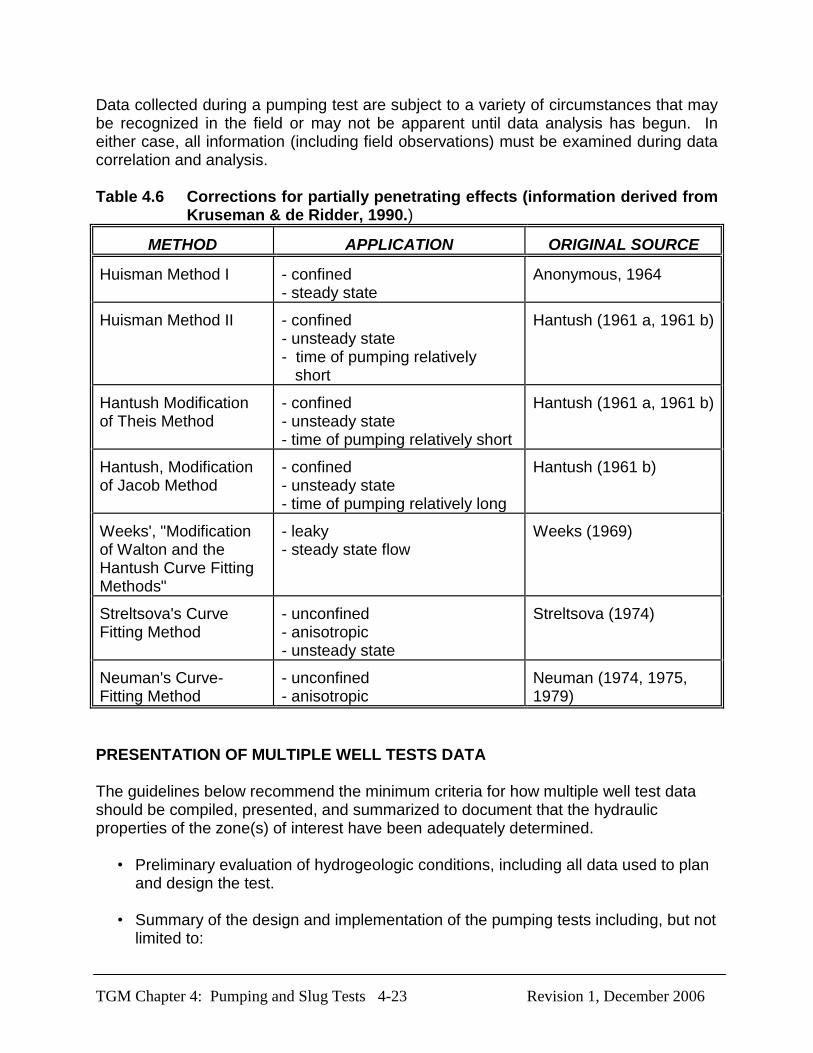
TGM Chapter 4: Pumping and Slug Tests 4-23 Revision 1, December 2006
Data collected during a pumping test are subject to a variety of circumstances that may be recognized in the field or may not be apparent until data analysis has begun. In either case, all information (including field observations) must be examined during data correlation and analysis. Table 4.6 Corrections for partially penetrating effects (information derived from
Kruseman & de Ridder, 1990.)
METHOD APPLICATION ORIGINAL SOURCE
Huisman Method I - confined - steady state
Anonymous, 1964
Huisman Method II - confined - unsteady state - time of pumping relatively short
Hantush (1961 a, 1961 b)
Hantush Modification of Theis Method
- confined - unsteady state - time of pumping relatively short
Hantush (1961 a, 1961 b)
Hantush, Modification of Jacob Method
- confined - unsteady state - time of pumping relatively long
Hantush (1961 b)
Weeks', "Modification of Walton and the Hantush Curve Fitting Methods"
- leaky - steady state flow
Weeks (1969)
Streltsova's Curve Fitting Method
- unconfined - anisotropic - unsteady state
Streltsova (1974)
Neuman's Curve-Fitting Method
- unconfined - anisotropic
Neuman (1974, 1975, 1979)
PRESENTATION OF MULTIPLE WELL TESTS DATA The guidelines below recommend the minimum criteria for how multiple well test data should be compiled, presented, and summarized to document that the hydraulic properties of the zone(s) of interest have been adequately determined.
• Preliminary evaluation of hydrogeologic conditions, including all data used to plan and design the test.
• Summary of the design and implementation of the pumping tests including, but not
limited to:

TGM Chapter 4: Pumping and Slug Tests 4-24 Revision 1, December 2006
Geologic zone into which the pumping well is completed (i.e. areal extent, thickness, lateral and vertical extent).
Pumping well construction (justification should be provided if the well screen is partially penetrating).
Duration of pumping.
Rate of pumping and method for determination.
Location of all observation wells. Geologic zone(s) to be monitored (including depths, thickness, spatial relationship to the pumped zone).
Observation and pumping well construction.
Method of water level measurements (for each well).
Methods for gathering data used to correct drawdown and establishment of existing trends in water levels.
Procedures for the discharge and disposal (if necessary) of pumped water.
Date and time pumping began and ended.
$ Raw data, including water level measurements, time of measurement in minutes
after pumping started or ended, drawdown, pumping rates, etc. should be included in tabular form. All data should be expressed in consistent units. Water level in nearby surface water bodies should also be provided, if taken. If the data set is large, it may be provided on disk.
• Data plots and type curves. All graphs and data plots should be labeled clearly.
Data plots of (e.g., drawdown versus time) should be presented for the pumping well and each observation well on double-logarithmic and semi-logarithmic paper. Time data (in minutes) should be depicted along the horizontal axis, and drawdown should be depicted along the vertical axis. For semi-logarithmic plots, drawdown should be presented along the vertical arithmetic axis.
The horizontal scale should be the same for all data plots.
All data points on the plots should be clearly labeled. In the event that data from multiple wells are presented on the same plot, the labeling should be distinct so as to enable differentiation between sets of data, and be identified in a legend.
TGM Chapter 4: Pumping and Slug Tests 4-25 Revision 1, December 2006
Data plots of drawdown versus distance from the pumping well should be presented; calculations of hydraulic properties based on these plots should be used to corroborate calculations made from time drawdown data plots. Data plots of residual drawdown versus time since pumping stopped should be presented for recovery data.
Data plots of discharge rate versus time should be presented.
For data depicted on double-logarithmic plots, the following requirements should be met: If a single type curve has been used to analyze the data, the type curve should be presented directly on the data plot.
If an analysis method employing a family of type curves has been used, all curves selected to fit the data (including both early and late time responses to pumping, if applicable) should be depicted directly on the data plot, and a discussion addressing the applicability of using multiple type curves should be included in the site investigation report.
Match point values should be identified on data plots.
For data depicted on semi-logarithmic plots, the portion of the data to which a straight line is fit should be indicated on the plot.
• Calculations. Equations used for calculating hydraulic properties should also be
included in the report. • In the event that any boundaries are encountered by the cone of depression
during the test, the report should contain (1) a reference to the data plot on which the boundary's impact can be observed, (2) identification of the type of boundary, and (3) a discussion addressing the boundary's effect on the hydraulics at the site. For pumping wells, an evaluation of casing storage effects should be included
• Comments noting any external events (e.g., change in weather patterns, passage
of train or heavy machinery). In the event that drawdown data need adjustment due to external effects or reduction in saturated thickness, separate data plots depicting both adjusted and unadjusted drawdown versus time and versus distance should be presented for the appropriate wells. Any plots, graphs, or equations used to determine the magnitude of drawdown adjustment should also be presented.
. • Data analysis method and/or programs, including assumptions, limitations and
their applicability to the site. • In the event that a computer program is used to perform the analysis, only those
software programs that provide analysis of the data based on graphical curve matching, rather than least-squares analysis, and allow for the generation of data plots should be used.

TGM Chapter 4: Pumping and Slug Tests 4-26 Revision 1, December 2006
• Interpretation of the data using both results of the test and other available hydrogeologic information.
RECOVERY TESTS Recovery tests (also called residual drawdown tests) involve measuring water level rise after the pump is shut down. These tests provide an independent check on the transmissivity and storativity determined from a pumping test. The results should be used in conjunction with calculations obtained from the pumping phase to estimate the true hydraulic properties of the zone(s) of interest. Results of a recovery test can be more reliable than pumping test results because recovery is not influenced by the erratic fluctuations that can be characteristic of pumping. As with the early portions of the pumping phase in which water levels drop rapidly, water levels rise rapidly during early portions of the recovery phase and are followed by a decreasing rate of water level rise. It is therefore important to establish the same schedule for obtaining water level measurements during the initial portions of the recovery phase as that used during the pumping phase (Kruseman and de Ridder, 1990. Table 4.12 provides methods for analyzing recovery data. At a minimum, the following information should be provided: date and time the pumping phase ended and the recovery phase began, initial and final water levels for the recovery phase, time since pumping stopped (in minutes), measured water level, residual drawdown, and records of any noteworthy occurrences.

TGM Chapter 4: Pumping and Slug Tests 4-27 Revision 1, December 2006
Table 4.7 Multiple-well, constant discharge pumping tests, unconfined aquifer ground water zone.
GENERAL ASSUMPTIONS 1. The ground water zone is unconfined and bounded below by an aquiclude. 2. All layers are horizontal and extend infinitely in the radial extent. 3. The ground water zone is homogeneous, isotropic (unless noted) and of uniform thickness. 4. Prior to pumping, the water table is horizontal over the area that will be influenced by the test. 5. Ground water density and viscosity are constant. 6. Ground water flow can be described by Darcy's Law. 7. Head losses through well screen and pump intake are negligible. 8. The ground water zone is compressible and completely elastic. 9. The zone has been pumped long enough that equilibrium has been reached. 10. Drawdown is small compared to the saturated thickness (i.e., no more than 25 percent). 11. Pumping and observation wells are screened over the entire saturated thickness (unless noted). 12. Ground water flow above the water table is negligible.
METHOD
CAN ACCOUNT FOR
REMARKS Flow Conditions
Partial Penetration
Other
Neuman's Curve Fitting Method (Neuman, 1972) (a,b)
Transient
No
anisotropic conditions
Theory should be valid for piezometers with short screens provided that the drawdowns are averaged over the saturated thickness (Van der Kamp, 1985)
Thiem-Dupuit's Method, (Thiem, 1906) (b)
Steady state
No
Steady state will only be achieved after long pumping time Does not give accurate description of drawdown near the well Assumptions ignore the existence of a seepage face at the well and the influence of the vertical velocity component
Boulton and Streltsova (1976) a
Transient Yes storage in the well
anisotropy
Neuman (1974) a Transient Yes anisotropy a Described in Dawson and Istok, 1991 b Described in Kruseman and de Ridder, 1990 t = time, = transmissivity, r = radial distance from the pumping well, rw = effective radius of the pumping well, rc= inside radius of the pumping well within the range of water fluctuations
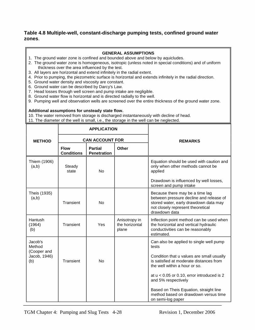
TGM Chapter 4: Pumping and Slug Tests 4-28 Revision 1, December 2006
Table 4.8 Multiple-well, constant-discharge pumping tests, confined ground water zones.
GENERAL ASSUMPTIONS 1. The ground water zone is confined and bounded above and below by aquicludes. 2. The ground water zone is homogeneous, isotropic (unless noted in special conditions) and of uniform
thickness over the area influenced by the test. 3. All layers are horizontal and extend infinitely in the radial extent. 4. Prior to pumping, the piezometric surface is horizontal and extends infinitely in the radial direction. 5. Ground water density and viscosity are constant. 6. Ground water can be described by Darcy's Law. 7. Head losses through well screen and pump intake are negligible. 8. Ground water flow is horizontal and is directed radially to the well. 9. Pumping well and observation wells are screened over the entire thickness of the ground water zone. Additional assumptions for unsteady state flow. 10. The water removed from storage is discharged instantaneously with decline of head. 11. The diameter of the well is small, i.e., the storage in the well can be neglected.
METHOD
APPLICATION
REMARKS CAN ACCOUNT FOR
Flow Conditions
Partial Penetration
Other
Thiem (1906) (a,b)
Steady state
No
Equation should be used with caution and only when other methods cannot be applied Drawdown is influenced by well losses, screen and pump intake
Theis (1935) (a,b)
Transient
No
Because there may be a time lag between pressure decline and release of stored water, early drawdown data may not closely represent theoretical drawdown data
Hantush (1964) (b)
Transient
Yes
Anisotropy in the horizontal plane
Inflection point method can be used when the horizontal and vertical hydraulic conductivities can be reasonably estimated.
Jacob's Method (Cooper and Jacob, 1946) (b)
Transient
No
Can also be applied to single well pump tests Condition that u values are small usually is satisfied at moderate distances from the well within a hour or so. at u < 0.05 or 0.10, error introduced is 2 and 5% respectively Based on Theis Equation, straight line method based on drawdown versus time on semi-log paper
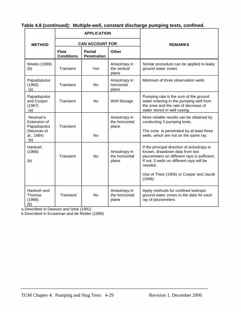
Table 4.8 (continued): Multiple-well, constant discharge pumping tests, confined.
TGM Chapter 4: Pumping and Slug Tests 4-29 Revision 1, December 2006
METHOD
APPLICATION
REMARKS CAN ACCOUNT FOR
Flow Conditions
Partial Penetration
Other
Weeks (1969) (b)
Transient
Yes
Anisotropy in the vertical plane
Similar procedure can be applied to leaky ground water zones
Papadopulos (1965) (a)
Transient
No
Anisotropy in horizontal plane
Minimum of three observation wells
Papadopulos and Cooper (1967) (a)
Transient
No
Well Storage
Pumping rate is the sum of the ground water entering in the pumping well from the zone and the rate of decrease of water stored in well casing.
Neuman's Extension of Papadopulos (Neuman et al., 1984) (b)
Transient
No
Anisotropy in the horizontal plane
More reliable results can be obtained by conducting 3 pumping tests. The zone is penetrated by at least three wells, which are not on the same ray.
Hantush (1966) (b)
Transient
No
Anisotropy in the horizontal plane
If the principal direction of anisotropy is known, drawdown data from two piezometers on different rays is sufficient. If not, 3 wells on different rays will be needed. Use of Theis (1906) or Cooper and Jacob (1946)
Hantush and Thomas (1966) (b)
Transient
No
Anisotropy in the horizontal plane
Apply methods for confined isotropic ground water zones to the data for each ray of piezometers
a Described in Dawson and Istok (1991) b Described in Kruseman and de Ridder (1990)
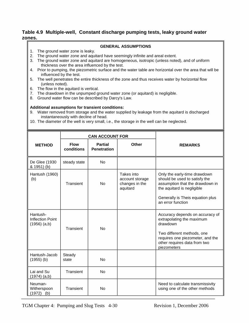
TGM Chapter 4: Pumping and Slug Tests 4-30 Revision 1, December 2006
Table 4.9 Multiple-well, Constant discharge pumping tests, leaky ground water zones.
GENERAL ASSUMPTIONS 1. The ground water zone is leaky. 2. The ground water zone and aquitard have seemingly infinite and areal extent. 3. The ground water zone and aquitard are homogeneous, isotropic (unless noted), and of uniform
thickness over the area influenced by the test. 4. Prior to pumping, the piezometric surface and the water table are horizontal over the area that will be
influenced by the test. 5. The well penetrates the entire thickness of the zone and thus receives water by horizontal flow
(unless noted). 6. The flow in the aquitard is vertical. 7. The drawdown in the unpumped ground water zone (or aquitard) is negligible. 8. Ground water flow can be described by Darcy's Law. Additional assumptions for transient conditions: 9. Water removed from storage and the water supplied by leakage from the aquitard is discharged
instantaneously with decline of head. 10. The diameter of the well is very small, i.e., the storage in the well can be neglected.
METHOD
CAN ACCOUNT FOR
REMARKS Flow conditions
Partial Penetration
Other
De Glee (1930 & 1951) (b)
steady state No
Hantush (1960) (b)
Transient
No
Takes into account storage changes in the aquitard
Only the early-time drawdown should be used to satisfy the assumption that the drawdown in the aquitard is negligible Generally is Theis equation plus an error function
Hantush-Inflection Point (1956) (a,b)
Transient
No
Accuracy depends on accuracy of extrapolating the maximum drawdown Two different methods, one requires one piezometer, and the other requires data from two piezometers
Hantush-Jacob (1955) (b)
Steady state
No
Lai and Su (1974) (a,b)
Transient No
Neuman-Witherspoon (1972) (b)
Transient
No
Need to calculate transmissivity using one of the other methods

Table 4.9 (continued). Multiple-well, constant discharge, pumping tests, leaky.
TGM Chapter 4: Pumping and Slug Tests 4-31 Revision 1, December 2006
METHOD
CAN ACCOUNT FOR
REMARKS Flow conditions
Partial Penetration
Other
Hantush-Jacob (1955) (a)
Transient
No
Drawdown in the source bed can be neglected when KD of source bed is >100 KD of ground water zone Ground water zone is bounded above by aquitard and an unconfined ground water zone and bounded below by an aquiclude Ground water flow in the aquitard is vertical
Walton (1962) (b)
Transient No
To obtain the unique fitting position of the data plot with one of the type curves, enough of the observation data should fall within the period when leakage effects are negligible
Hantush (1966) (b)
Transient No
Anisotropic in horizontal plane
Similar to Hantush's methods for confined zone except initial step uses methods to calculate the hydraulic parameters
Weeks (1969) (b)
Transient Yes Anisotropic in the vertical plane
Similar process can be conducted for confined zone
a Described in Dawson and Istok, 1991 b Described in Kruseman and de Ridder, 1990 t = time since start of pumping, S' = aquitard storativity, D'= saturated thickness of aquitard, D = saturated thickness of the ground water zone, K'= hydraulic conductivity of aquitard

TGM Chapter 4: Pumping and Slug Tests 4-32 Revision 1, December 2006
Table 4.10 Pumping tests, variable discharge.
METHOD* APPLICATION ASSUMPTIONS REMARKS
Birsoy and Summers (1980)
-Confined -Transient -Pumped step-wise or intermittently at variable rates
-General assumptions for confined ground water zones
Tedious process
Aron and Scott (1965)
-Confined -Transient Discharge rate decreases
-General assumptions for confined ground water zones
-Discharge rate deceases with time sharpest decrease occurring soon after the start of pumping
Analogous to the Jacob Method
Hantush (1964) -Confined
-Transient
-Standard assumptions for confined ground water zones
-At the start of the tests, the water level in the free flowing well drops instantaneously. At t> 0 drawdown is constant and its discharge rate is variable
Hantush-De Glee Method (Hantush, 1959b)
-Leaky
-Transient
-Fully penetrating well
-Standard assumptions for leaky ground water zones (see leaky section)
-At the start of the tests, the water level in the free flowing well drops instantaneously. At t >0 drawdown is constant and its discharge rate is variable
* Methods described in Kruseman and de Ridder (1990).

TGM Chapter 4: Pumping and Slug Tests 4-33 Revision 1, December 2006
Table 4.11 Methods of analysis for pumping tests with special conditions.
GROUND WATER ZONE CONDITION
FLOW TYPE MODELS & SOURCES2
One or more recharge boundaries
Steady State Confined or Unconfined
Dietz (1943)
One or more straight recharge boundaries
Unsteady State Confined or Unconfined
Stallman (in Ferris et al., 1962)
One recharge boundary Unsteady State Confined or Unconfined
Hantush (1959a)
Bounded by two fully penetrating boundaries
Unsteady State Leaky or Confined
Vandenberg (1976 and 1977)
Wedge shaped ground water zones
Unsteady State Confined Hantush (1962)
Water table slopes
Steady State Unconfined Culmination Point Method (Huisman, 1972)
Unsteady State Unconfined Hantush (1964)
Two layered ground water zone, unrestricted cross flow Pumping well does not penetrate entire thickness
Unsteady State
Confined
Javandel-Witherspoon (1983)
Leaky two-layered ground water zone , separated by aquitard with cross-flow across aquitard
Steady State Leaky Bruggeman (1966)
Large diameter well Unsteady State Confined Papadopulos (1967), Papadopulos and Cooper (1967)
Large diameter well Unsteady State Unconfined Boulton and Streltsova, (1976)
2 Methods are described in Kruseman and de Ridder, 1990.

TGM Chapter 4: Pumping and Slug Tests 4-34 Revision 1, December 2006
Table 4.12 Recovery test methods (discussed in Kruseman and de Ridder, 1990).
METHOD APPLICATION SOURCE
Theis Recovery Methods
Confined Unsteady state Recovery after constant discharge
Theis (1935)
Leaky Unsteady state Recovery after constant discharge
Vandenberg (1975) Hantush (1964)
Unconfined Recovery after constant discharge Late recovery data
Neuman (1975)
Unconfined Recovery after constant drawdown
Rushton and Rathod (1980)
Birsoy and Summers
Unconfined Recovery after variable discharge
Birsoy and Summers (1980)

TGM Chapter 4: Pumping and Slug Tests 4-35 Revision 1, December 2006
REFERENCES Anonymous, 1964. Steady Flow of Groundwater Towards Wells. Proc. Comm.
Hydrology. Research TNO No.10. Cited in Kruseman and de Ridder, 1990. Aron, G. and V. H. Scott. 1965. Simplified Solution For Decreasing Flow Into Wells.
American Society of Civil Engineers Proceedings. Vol. 91, No. HY5, pp. 1-12. American Society for Testing and Materials (ASTM), Method D4043-96 (2004).
Standard Guide for the Selection of Aquifer-Test Methods in Determining the Hydraulic Properties by Well Techniques. Conshohocken, Pennsylvania.
ASTM, Method D4044-96(2002). Standard Test Method (Field Procedure) for
Instantaneous Change in Head (Slug Tests) for Determining Hydraulic Properties of Aquifers. Conshohocken, Pennsylvania.
ASTM, Method D4104-96 (2004). Standard Test Method (Analytical Procedure) for
Determining Transmissivity of Nonleaky Confined Aquifers by Overdamped Well Response to Instantaneous Change in Head (Slug Test). Conshohocken, Pennsylvania.
ASTM, Method D4105-96(2002). Standard Test Method (Analytical Procedure) for
Determining Transmissivity and Storage Coefficient of Nonleaky Confined Aquifers by the Modified Theis Nonequilibrium Method. Conshohocken, Pennsylvania.
ASTM, Method D4106-96 (2004). Standard Test Method (Analytical Procedure) for
Determining Transmissivity and Storage Coefficient of Nonleaky Confined Aquifers by the Modified Theis Nonequilibrium Method. Conshohocken, Pennsylvania.
ASTM, Method D4361-95 (2000). Standard Test Method for Determining Transmissivity
and Storativity of Low Permeability Rocks by In Situ Measurements Using Pressure Pulse Technique Conshohocken, Pennsylvania.
ASTM, Method D4750-87(2001). Standard Test Method for Determining Subsurface
Liquid Levels in a Borehole or Monitoring Well (Observation Well). Conshohocken, Pennsylvania.
Batu, Vedat. 1998. Aquifer Hydraulics: A Comprehensive Guide to Hydrogeologic Data
Analysis. John Wiley & Sons, Inc. 727pp. Birsoy, Y. K. and W. K. Summers. 1980. Determination of Aquifer Parameters From
Step Tests and Intermittent Pumping Data. Ground Water. Vol. 18, No. 2, pp. 137-146.
Black, J. H. 1978. The Use of Slug Tests in Ground Water Investigations. Water
Services. pp. 174-178.
TGM Chapter 4: Pumping and Slug Tests 4-36 Revision 1, December 2006
Boulton, N. S. and T. D. Streltsova. 1976. The Drawdown Near an Abstraction of Large Diameter Under Non-Steady State Conditions in Unconfined Aquifers. Journal of Hydrology. Vol. 30, pp. 29-46.
Bouwer, H. and R. C. Rice. 1976. A Slug Test For Determining Hydraulic Conductivity
of Unconfined Aquifers with Complete or Partially Penetrating Wells. Water Resources Research. Vol. 12, No. 3, pp. 423-428.
Bouwer, H. 1989. The Bouwer and Rice Slug Test--An Update. Ground Water. Vol.
27, No. 3, pp. 304-309. Bredehoeft, J. D. and S. S. Papadopulos. 1980. A Method for Determining Hydraulic
Properties of Tight Formations. Water Resources Research. Vol. 16, No. 1, pp. 233-238.
Bruggeman, G. A. 1966. Analyse van de Bodemconstanten in een Grondpakket,
Bestaande Uit Twee of Meer Watervoerende Lagen Gescheiden door Semi-Permeabele Lagen. Unpublished Research Paper. Cited in Kruseman and de Ridder, 1990.
Butler, J.J. 1998. The Design and Performance, and Analysis of Slug Tests. Lewis
Publishers (imprint of CRC Press LLC.) Boca Raton, Florida. 252 pp. Chirlin, G.R. 1990. The Slug Test: The First Four Decades. Ground Water
Management. Proceedings of the 1990 Cluster Conference. National Water Well Association. Columbus, Ohio. pp. 365-381.
Cooper, H. H., J. D. Bredehoeft, and I. S Papadopulos. 1967. Response of a Finite-
Diameter Well to an Instantaneous Charge of Water. Water Resources Research. Vol. 3, No. 1, pp. 263-269.
Cooper, H. H. and C. E. Jacob. 1946. A Generalized Graphical Method for Evaluating
Formation Constants and Summarizing Well Field History. Transactions of the American Geophysical Union. Vol. 24, No. 4, pp. 526-534.
Dalton, M. G., B. E. Huntsman, and K. Bradbury. 2006. Acquisition and Interpretation
of Water-Level Data. In: D. M. Nielsen (editor), Practical Handbook of Ground-Water Monitoring. Lewis Publishers, Inc. Chelsea, Michigan. pp.883-911.
Dawson, K. and J. D. Istok. 1991. Aquifer Testing, Design and Analysis of Pumping
and Slug Tests. Lewis Publishers, Inc. Chelsea, Michigan. De Glee, G. J. 1930. Over Grondwaterstromingen bij Wateronttrekking Door Middel
Van Putten. Thesis. J. Waltman, Delft (The Netherlands). Cited in Kruseman and de Ridder (1990).
TGM Chapter 4: Pumping and Slug Tests 4-37 Revision 1, December 2006
De Glee, G. J. 1951. Berekeningsmethoden voor de Winning van Grondwater. In: Drinkwatervoorziening, 3e Vacantiecursus: 38-80 Moorman's Periodieke pers. The Hague. Cited in Kruseman and de Ridder, 1990.
Dietz, D. N. 1943. De Toepassing van Invloedsfuncties bij het Berekenen van de
Verlaging van het Grondwater ten Gevolge van Wateronttrekking. Water. Vol. 27(6), pp. 51-54. Cited in Kruseman and de Ridder, 1990.
Domenico, P.A. and F.W. Schwartz. 1998. Second Edition. Physical and Chemical
Hydrogeology. John Wiley and Son, Inc. New York. Driscoll, F. G. (editor). 1986. Groundwater and Wells. Second Edition. Wheelabrator
Engineered Systems-Johnson screens. St. Paul, Minnesota. Fetter, C. W. 2001. Applied Hydrogeology. Fourth Edition. Prentice Hall. Uper
Saddle River, New Jersey. Ferris, J. G., D. B. Knowles, R. H. Brown, and R. W. Stallman. 1962. Theory of Aquifer
Tests. U.S. Geological Survey, Water-Supply Paper 1536E. Hantush, M. S. 1956. Analysis of Data From Pumping Tests in Leaky Aquifers.
Transactions of the American Geophysical Union. Vol. 37, No. 6, pp. 702-714. Hantush, M. S. 1959a. Analysis of Data From Pumping Well Near a River. Journal of
Geophysical Research. Vol. 94, pp. 1921-1923. Hantush, M. S. 1959b. Non-Steady Flow to Flowing Wells in Leaky Aquifers. Journal
of Geophysical Research. Vol. 64, No. 8, pp. 1043-1052. Hantush, M. S. 1960. Modification of the Theory of Leaky Aquifers. Journal of
Geophysical Research. Vol.65, No. 11, pp. 3713-3725. Hantush, M. S. 1961a. Drawdown Around a Partially Penetrating Well. Journal of the
Hydraulics Division. Proceedings of the American Society of Civil Engineers. Vol. 87 (HY4), pp. 83-98.
Hantush, M. S. 1961b. Aquifer Tests on Partially Penetrating Wells. Journal of the
Hydraulics Division. Proceedings of the American Society of Civil Engineers. Vol. 87(HY5), pp. 172-195.
Hantush, M. S. 1962. Flow of Ground Water in Sands of Nonuniform Thickness-- Part
3, Flow to Wells. Journal of Geophysical Research. Vol. 67, No. 4, pp. 1527-1534. Hantush, M. S. 1964. Hydraulics of Wells. In: V. T. Chow (editor), Advances in
Hydrosciences. Vol. 1. Academic Press. London and New York. pp. 281-442.
TGM Chapter 4: Pumping and Slug Tests 4-38 Revision 1, December 2006
Hantush, M. S. 1966. Analysis of Data From Pumping Tests In Anisotropic Aquifers. Journal of Geophysical Research. Vol. 71, No. 2, pp. 421-426.
Hantush, M. S. and C. E. Jacob. 1955. Non-Steady State Radial Flow in an Infinite
Leaky Aquifer. Transactions of the American Geophysical Union. Vol. 36, No. 1, pp. 95-100.
Hantush, M. S. and R. G. Thomas. 1966. A Method for Analyzing a Drawdown Test in
Anisotropic Aquifers. Water Resources Research. Vol. 2, No. 2, pp. 281-285. Huisman, L. 1972. Groundwater Recovery. MacMillan. Hvorslev, M. J. 1951. Time Lag and Soil Permeability in Groundwater Observation.
U.S. Army Corps of Engineers, Waterways Experiment Station. Bulletin No. 36. Vicksburg, Mississippi.
Jacob, C. E. 1944. Notes on Determining Permeability by Pumping Tests Under Water Table Conditions. U.S. Geological Survey. Open file report.
Jacob, C. E. and S. W. Lohman. 1952. Non-Steady Flow to a Well of Constant
Drawdown in an Extensive Aquifer. Transactions of the American Geophysical Union. Vol. 33, pp. 559-569.
Javandel, I. and R. A. Witherspoon. 1983. Analytical Solution of a Partially Penetrating
Well in a Two-Layer Aquifer. Water Resources Research. Vol 19., pp. 567-578. Kruseman, G. P. and de Ridder, N. A. 1990. Analysis and Evaluation of Pumping Test
Data. Second Edition. International Institute for Land Reclamation and Improvement (ILRI) Publication 47. Wageningen, The Netherlands.
Lai, R. Y. S. and C. W. Su. 1974. Nonsteady Flow to a Large Diameter Well in a Leaky
Aquifer. Journal of Hydrology. Vol. 22. pp. 333-345. Lohman, S. W. 1972. Groundwater Hydraulics. U.S. Geological Survey Professional
Paper 708. United States Government Printing Office. Washington, D.C. Neuman, S. P. 1972. Theory of Flow in Unconfined Aquifers Considering Delayed
Response of the Water Table. Water Resources Research. Vol. 8, No 4, pp. 1031-1045.
Neuman, S. P. 1974. Effects of Partial Penetration on Flow in Unconfined Aquifers Considering Delayed Gravity Response. Water Resources Research. Vol. 10, No 2, pp. 303-312. Neuman, S. P. 1975. Analysis of Pumping Test Data From Anisotropic Unconfined
Aquifers Considering Delayed Gravity Response. Water Resources Research. Vol. 11, No, 2, pp. 329-342.
TGM Chapter 4: Pumping and Slug Tests 4-39 Revision 1, December 2006
Neuman, S. P. 1979. Perspective on 'Delayed Yield'. Water Resources Research. Vol. 15, No. 4, pp. 899-908.
Neuman, S. P. and P. A. Witherspoon. 1972. Field Determination of the Hydraulic
Properties of Leaky Multiple Aquifer Systems. Water Resources Research. Vol. 8, No. 5, pp. 1284-1298.
Neuman, S. P., G. R. Walter, H. W. Bentley, J. J. Ward and D. D. Gonzalez. 1984.
Determination of Horizontal Anisotropy With Three Wells. Ground Water. Vol. 22, No. 1, pp. 66-72.
Orient, J. P., A. Nazar and R.C. Rice. 1987. Vacuum and Pressure Test Methods for
Estimating Hydraulic Conductivity. Ground Water Monitoring Review. Vol. 7, No. 1, pp. 49-50.
Osborne, P. S. 1993. Suggested Operating Procedures for Aquifer Pumping Tests.
U.S.EPA. Office of Research and Development, Office of Solid Waste. EPA/540/S-93/503.
Papadopulos, I. S. 1965. Nonsteady flow to a well in a finite anisotropic aquifer. International Association of Scientific Hydroglogy Symposium. American Water Resources Assoc. Proc. No. 4, pp. 157-168. Papadopulos, I. S. 1967. Drawdown Distribution Around a Large Diameter Well.
Symposium on Groundwater Hydrology. Proceedings of American Water Resources. No. 4, pp. 157-168.
Papadopulos, I. S. and H. H. Cooper. 1967. Drawdown in Large Diameter Wells.
Water Resources Research. Vol. 3, No. 1, pp. 241-244. Rushton, K. R. and K. S. Rathod. 1980. Overflow Tests Analyzed by Theoretical and
Numerical Methods. Ground Water. Vol. 18, No. 1, pp. 61-69. Rushton, K. R. and V. S. Singh. 1983. Drawdowns in Large-diameter Wells Due To
Decreasing Abstraction Rates. Ground Water. Vol. 21, No. 6, pp. 671-677. Sara, M.C. 2003. Site Assessment and Remediation Handbook. Second Edition. CRC
Press, Lewis Publications. Sevee, J. 2006. Methods and Procedures for Defining Aquifer Parameters. In: D. M.
Nielsen (editor), Practical Handbook of Ground-Water Monitoring. Taylor & Francis Group, CRC Press, Boca Raton, Fl. pp. 913-958.
Stallman, R. W. 1983. Aquifer-Test Design, Observation and Data Analysis: U.S.
Geological Survey Techniques of Water-Resource Investigations, Book 3, Chapter B1. United States Government Printing Office. Washington, D. C.

TGM Chapter 4: Pumping and Slug Tests 4-40 Revision 1, December 2006
Streltsova, T. D. 1974. Drawdown in Compressible Unconfined Aquifer. Journal of the Hydraulics Division. American Society of Civil Engineers. HYll, pp. 1601-1616.
Theis, C. V. 1935. The Relation Between the Lowering of the Piezometric Surface and
the Rate and Duration of Discharge of a Well Using Groundwater Storage. Transactions of the American Geophysical Union. Vol. 16, pp. 519-524.
Thiem, G. 1906. Hydrologische Methoden. Gebhardt. Leipzig. Cited in Kruseman and
de Ridder, 1990. Uffink, G. J. M. 1984. Theory of the Oscillating Slug Test. National Institute for Public
Health and Environmental Hygiene Bilthoven. Unpublished research report (in Dutch). Cited in Kruseman and de Ridder, 1990.
U.S. EPA. 1986. Saturated Hydraulic Conductivity, Saturated Leachate Conductivity
and Intrinsic Permeability. In: Test Methods for Evaluating Solid Waste. SW846, Method 9100. Office of Solid Waste and Emergency Response. U.S. Environmental Protection Agency. Washington, D.C.
Vandenberg, A. 1975. Determining Aquifer Coefficients From Residual Drawdown
Data. Water Resources Research. Vol. 11, pp. 1025-1028. Vandenberg, A. 1976. Tables and Types Curves for Analysis of Pumping Tests in
Leaky Parallel-Channel Aquifers. Technical Bulletin No. 96. Inland Waters Directorate, Water Resource Branch. Ottawa (Canada).
Vandenberg, A. 1977. Type Curve Analysis of Pump Tests in Leaky Strip Aquifers.
Journal of Hydrology. Vol. 33, pp. 15-26. Van der Kamp, G. 1985. Brief Quantitative Quidelines for Design and Analysis of Pumping Tests. In: Hydrology in the Service of Man. Memoirs of the 18th Congress Intern. Assoc. Hydrogeol. Cambridge, Massachusetts. pp. 197-206 Walton, W.C.1996. Aquifer Analysis with WINDOWSTM Software. Lewis Publishers,
CRC Press. 301pp. Walton, W. C. 1962. Selected Analytical Methods for Well and Aquifer Evaluation.
Illinois State Water Survey. Bulletin No. 49. Walton, W. C. 1987. Groundwater Pumping Tests, Design and Analysis. Lewis
Publishers, Inc. Chelsea, Michigan. Weeks, E. P. 1969. Determining the Ratio of Horizontal to Vertical Permeability by
Aquifer-Test Analysis. Water Resources Research. Volume 5, pp. 196-214. Worthington, P. F. 1981. Estimation of Transmissivity of Thin Leaky-Confined Aquifers
from Single-Well Pumping Test. Journal of Hydrology. Vol. 49, pp. 19-30.

State of Ohio Environmental Protection Agency
Division of Drinking and Ground Waters
Technical Guidance Manual for Ground Water Investigations Chapter 5
Monitoring Well Placement
November 2007 Governor : Ted Strickland Director : Chris Korleski
(Modified from U.S. EPA, 1993a)

TECHNICAL GUIDANCE MANUAL FOR
GROUND WATER INVESTIGATIONS
CHAPTER 5
MONITORING WELL PLACEMENT
November 2007 (Revision 1)
Ohio Environmental Protection Agency Division of Drinking and Ground Waters
P.O. Box 1049 50 West Town Street, Suite XXX Columbus, Ohio 43216-1049
Phone: 614-644-2752 http://www.epa.state.oh.us/ddagw/

TGM: Chapter 5: Monitoring Well Placement 5-ii Revision 1, November 2007
PREFACE
This document is part of a series of chapters incorporated in Ohio EPA’s Technical Guidance Manual for Hydrogeologic Investigations and Ground Water Monitoring (TGM), which was originally published in 1995. DDAGW now maintains this technical guidance as a series of chapters rather than as an individual manual. These chapters can be obtained at http://www.epa.state.oh.us/ddagw/tgmweb.aspx. The TGM identifies technical considerations for performing hydrogeologic investigations and ground water monitoring at potential or known ground water pollution sources. The purpose of the guidance is to enhance consistency within the Agency and inform the regulated community of the Agency’s technical recommendations and the basis for them. In Ohio, the authority over pollution sources is shared among various Ohio EPA divisions, including the Emergency and Remedial Response (DERR), Hazardous Waste Management (DHWM), Solid and Infectious Waste (DSIWM), and Surface Water (DSW), as well as other state and local agencies. DDAGW provides technical support to these divisions. Ohio EPA utilizes guidance to aid regulators and the regulated community in meeting laws, rules, regulations, and policy. Guidance outlines recommended practices and explains their rationale. The Agency may not require an entity to follow methods recommended by this or any other guidance document. It may, however, require an entity to demonstrate that an alternate method produces data and information that meet the pertinent requirements. The procedures used usually should be tailored to the specific needs and circumstances of the individual site, project, and applicable regulatory program, and should not comprise a rigid step-by-step approach that is utilized in all situations.

TGM: Chapter 5: Monitoring Well Placement 5-iii Revision 1, November 2007
TABLE OF CONTENTS PREFACE.............................................................................................................................. 5-ii TABLE OF CONTENTS ....................................................................................................... 5-iii ACKNOWLDEGEMENTS ..................................................................................................... 5-iv Changes from February 1995 TGM ...................................................................................... 5-v
FACTORS TO CONSIDER................................................................................................... 5-1 PUPOSE OF MONITORING ............................................................................................. 5-1 SITE HYDROGEOLOGY .................................................................................................. 5-1 CONTAMINANT PROPERTIES ........................................................................................ 5-5
DESIGN OF A MONITORING WELL NETWORK ................................................................ 5-9
NUMBER OF WELLS ..................................................................................................... 5-10 VERTICAL PLACEMENT................................................................................................ 5-10
Depth of Intakes .......................................................................................................... 5-10
Length of Intakes ......................................................................................................... 5-12
AREAL PLACEMENT OF DOWNGRADIENT WELLS ................................................... 5-13 Placement Relative to Pollution Source ...................................................................... 5-13 Spacing ....................................................................................................................... 5-14
BACKGROUND MONITORING WELL(S) PLACEMENT ................................................ 5-15 Location ....................................................................................................................... 5-15
Number........................................................................................................................ 5-16 REFERENCES ................................................................................................................... 5-17

TGM: Chapter 5: Monitoring Well Placement 5-iv Revision 1, November 2007
ACKNOWLEDGMENTS
This guidance was developed by Ohio EPA’s Division of Drinking and Ground Waters (DDAGW). The following are acknowledged for the preparation of this document. Lisa Koenig, DDAGW-CO, who had primary responsibility for this chapter. Jeff Patzke, DDAGW-CO, who serves as editor and project coordinator for the Technical Guidance Manual. The Ohio EPA would also like to thank the numerous people who provided input during its development. The comments and recommendations from the DDAGW-District Offices, and other Ohio EPA Divisions, state and federal agencies, private consultants, and regulated community were greatly appreciated.

TGM: Chapter 5: Monitoring Well Placement 5-v Revision 1, November 2007
Changes from February 1995 TGM
The Ohio EPA Technical Guidance Manual for Hydrogeologic Investigations and Ground Water Monitoring (TGM) was finalized in 1995. This guidance document represents an update to Chapter 5 (Monitoring Well Placement). No major technical changes were made to the chapter.

CHAPTER 5 MONITORING WELL PLACEMENT
Ground water quality at potential pollution sources can best be evaluated by chemical analysis of ground water samples collected from properly located, installed, and constructed monitoring wells. Several factors will dictate the placement of wells. For purposes of this document, the term, "monitoring well placement", refers to the areal location of a well and the depth and the length of its intake. In general, monitoring wells are placed to collect data representative of ground water at locations that are and are not likely to have been impacted from regulated activities or known or suspected sources of contaminants.
FACTORS TO CONSIDER Factors that should be considered when placing wells include: purpose of the monitoring, hydrogeologic/geologic characteristics, contaminant characteristics, and anthropogenic influences. In addition, budget and public interest may play a role. The configuration and size of contaminant plumes and/or number of pathways are composites of the hydrogeologic/geologic characteristics, contaminant characteristics, and anthropogenic influences. PURPOSE OF MONITORING Proper placement of monitoring wells is necessary to: 1) determine flow direction, 2) detect the release of contaminants from a suspected or known source, 3) determine the extent of contamination, 4) help design a remedy, 5) monitor the effectiveness and efficiency of a remedy, 6) act as a warning system to allow potential receptors to take action in the event of a plume advancement, and 7) determine concentrations of contaminants to assess the risk. Table 5.1 provides a brief discussion on some of the objectives associated with placement of wells.
SITE HYDROGEOLOGY Understanding the principles of ground water movement (flow rate, direction, and gradient) through various types of geologic materials plays a key role in developing strategies for identifying likely contaminant migration routes and selecting ground water monitoring locations. If the distribution and characteristics of materials are not defined, the zones requiring monitoring may be identified incorrectly, and releases may remain undetected. Hydrogeologic conditions affecting the placement of well intakes include: depth of water table, presence of perched water, subsurface materials (e.g., unconsolidated, bedrock), presence of multiple ground water zones, zone type (i.e., confined versus unconfined), presence of continuous zones that may restrict flow, type and amount of recharge and discharge, permeability, fractures, and capillary fringe. The components of a hydrogeologic investigation are outlined in Chapter 3.

TGM: Chapter 5: Monitoring Well Placement 5-2 Revision 1, November 2007
Table 5.1 Objectives of Ground Water Monitoring.
OBJECTIVE DISCUSSION
Detection/Compliance
Wells are placed at the downgradient boundary of a potential source to detect a release. These wells are used to determine that compliance requirements are being met according to some minimum or maximum standard.
Assessment Wells are placed progressively away from the potential source(s) to determine the rate and extent of contaminant migration. Monitoring often occurs at the fringes of the plume.
Risk Assessment
Monitoring to determine the concentrations within a plume to help determine the potential risk to human health and the environment. A toxicologist may require information concerning the reasonable maximum concentration of contaminants to assess risk at specific locations.
Warning System Wells are placed near a receptor to act as a warning system from any potential sources of contamination. Would allow the owner of potential receptors to take action.
Trend Analysis Designed to evaluate whether a decreasing or increasing trend is occurring. May be conducted to determine remedy progression or the effects of activities such as application of fertilizer.
Remedy Progression Wells are used to determine whether the remedy is working property.
Cause and Effect Wells are placed to evaluate an action or process (e.g. pumping of ground water.)
Preferential pathways for contaminant migration include zones that are fractured or have relatively high matrix hydraulic conductivity (K). The distribution of these materials can play a significant role in dictating ground water and contaminant movement. The presence of conductive zones within less conductive zones can create multiple paths of migration from a source. For example, Figure 5.1 shows a buried river channel. The regional and local ground water flow is toward the river; however, beneath a portion of the site, ground water is directed along the buried channel. Figure 5.2 demonstrates how water and contaminants may migrate horizontally across a perched water zone and then vertically through the unsaturated zone, transmitting contaminants to an underlying water-bearing zone over a pathway that is circuitous and not easily identified. Figure 5.3 demonstrates how complex flow patterns can occur due to fracturing. Regional and local flow is to the south. However, the orientation, density and connectivity of fractures may initially direct ground water and contaminants to the southeast, then southwest The processes controlling the movement of dissolved contaminants through porous media include advection, mechanical dispersion, and diffusion. Advection is the transport of solutes by the flowing ground water. Ground water moves at rates both greater and less than the average linear velocity. This is due to: 1) fluids moving faster through the center of the pores than along the edges, 2) fluids travelling shorter pathways and/or splitting or branching to the sides, and 3) fluids travelling faster through larger pores than through smaller pores (Fetter, 2001). Because the invading solute-containing water does not travel at the same velocity, mixing occurs along flow paths. This mixing is called mechanical dispersion and results in distribution of the solute at the advancing edge of flow (Fetter, 1999). The mixing that occurs in the direction of flow is called longitudinal dispersion. Spreading normal to the direction of flow from splitting and branching out to the sides is called transverse dispersion.

TGM: Chapter 5: Monitoring Well Placement 5-3 Revision 1, November 2007
Downgradient detection wells
Downgradient well in buried channel
Preferential pathway of contaminant migration into the buried river channel
Local ground-water flow direction Figure 5.1 Geologic setting where ground water flow is affected by a buried river channel. Ground water flow is regionally and locally directed toward the river; however over a portion of the site, the ground water is directed along a buried valley (Source: Modified from U.S. EPA, 1993a).
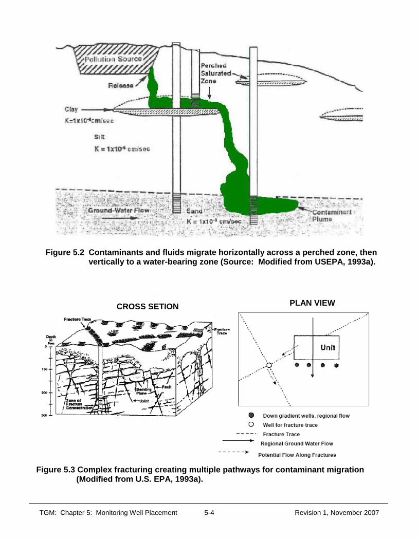
TGM: Chapter 5: Monitoring Well Placement 5-4 Revision 1, November 2007
Figure 5.2 Contaminants and fluids migrate horizontally across a perched zone, then
vertically to a water-bearing zone (Source: Modified from USEPA, 1993a).
Figure 5.3 Complex fracturing creating multiple pathways for contaminant migration
(Modified from U.S. EPA, 1993a).
CROSS SETION PLAN VIEW
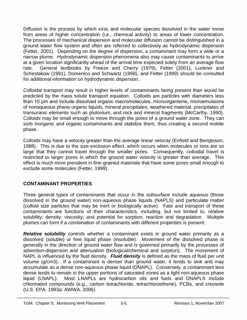
TGM: Chapter 5: Monitoring Well Placement 5-5 Revision 1, November 2007
Diffusion is the process by which ionic and molecular species dissolved in the water move from areas of higher concentration (i.e., chemical activity) to areas of lower concentration. The processes of mechanical dispersion and molecular diffusion cannot be distinguished in a ground water flow system and often are referred to collectively as hydrodynamic dispersion (Fetter, 2001). Depending on the degree of dispersion, a contaminant may form a wide or a narrow plume. Hydrodynamic dispersion phenomena also may cause contaminants to arrive at a given location significantly ahead of the arrival time expected solely from an average flow rate. General textbooks by Freeze and Cherry (1979), Fetter (2001), Luckner and Schestakow (1991), Domenico and Schwartz (1998), and Fetter (1999) should be consulted for additional information on hydrodynamic dispersion. Colloidal transport may result in higher levels of contaminants being present than would be predicted by the mass solute transport equation. Colloids are particles with diameters less than 10 μm and include dissolved organic macromolecules, microorganisms, microemulsions of nonaqueous phase organic liquids, mineral precipitates, weathered material, precipitates of transuranic elements such as plutonium, and rock and mineral fragments (McCarthy, 1990). Colloids may be small enough to move through the pores of a ground water zone. They can sorb inorganic and organic contaminants and stabilize them, thus creating a second mobile phase. Colloids may have a velocity greater than the average linear velocity (Enfield and Bengtsson, 1988). This is due to the size-exclusion effect, which occurs when molecules or ions are so large that they cannot travel through the smaller pores. Consequently, colloidal travel is restricted to larger pores in which the ground water velocity is greater than average. This effect is much more prevalent in fine-grained materials that have some pores small enough to exclude some molecules (Fetter, 1999).
CONTAMINANT PROPERTIES Three general types of contaminants that occur in the subsurface include aqueous (those dissolved in the ground water) non-aqueous phase liquids (NAPLS) and particulate matter (colloid size particles that may be inert or biologically active). Fate and transport of these contaminants are functions of their characteristics, including, but not limited to, relative solubility; density; viscosity; and potential for sorption, reaction and degradation. Multiple plumes can form if a combination of contaminants with different properties is present. Relative solubility controls whether a contaminant exists in ground water primarily as a dissolved (soluble) or free liquid phase (insoluble). Movement of the dissolved phase is generally in the direction of ground water flow and is governed primarily by the processes of advection-dispersion and attenuation (biological/chemical and sorption). The movement of NAPL is influenced by the fluid density. Fluid density is defined as the mass of fluid per unit volume (g/cm3). If a contaminant is denser than ground water, it tends to sink and may accumulate as a dense non-aqueous phase liquid (DNAPL). Conversely, a contaminant less dense tends to remain in the upper portions of saturated zones as a light non-aqueous phase liquid (LNAPL). Most LNAPLs are hydrocarbon oils and fuels and DNAPLS include chlorinated compounds (e.g., carbon tetrachloride, tetrachloroethene), PCBs, and creosote (U.S. EPA, 1993a; AWWA, 2006).
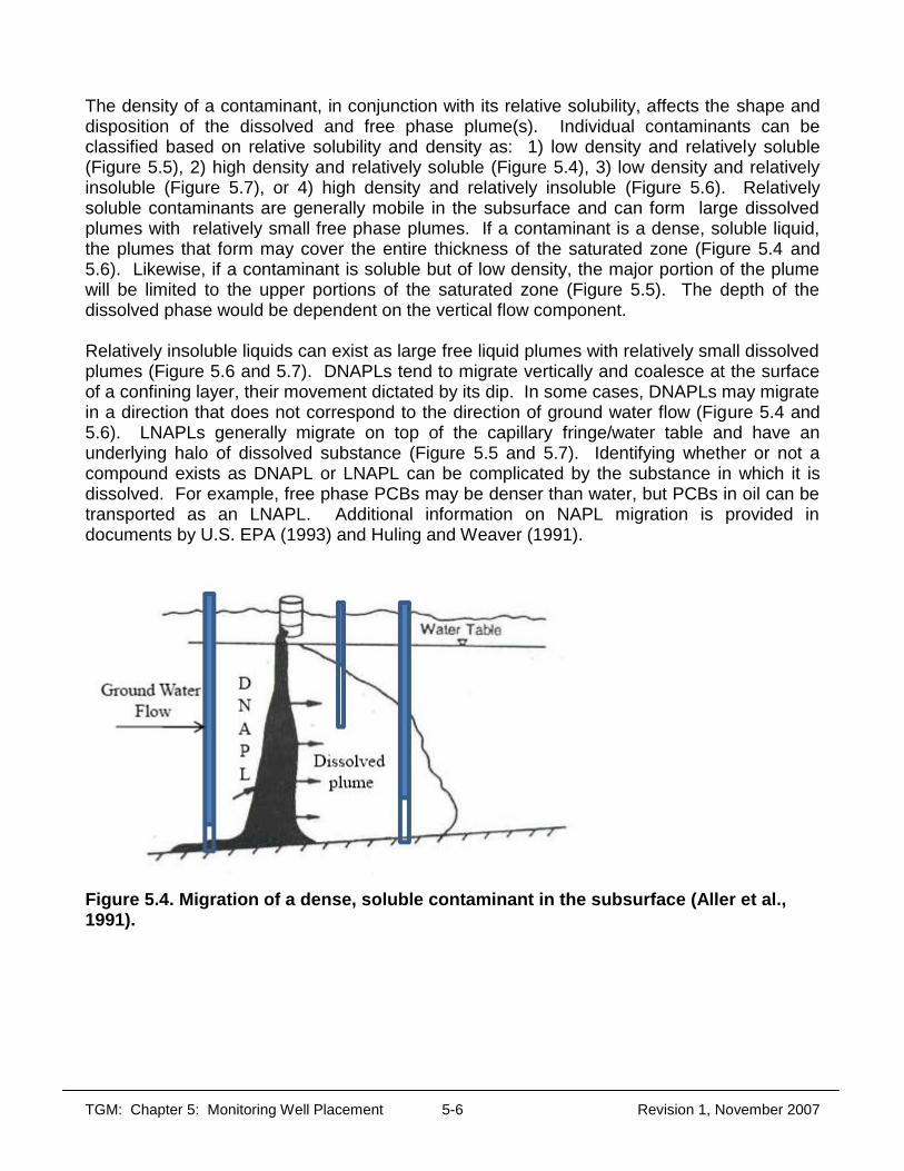
TGM: Chapter 5: Monitoring Well Placement 5-6 Revision 1, November 2007
The density of a contaminant, in conjunction with its relative solubility, affects the shape and disposition of the dissolved and free phase plume(s). Individual contaminants can be classified based on relative solubility and density as: 1) low density and relatively soluble (Figure 5.5), 2) high density and relatively soluble (Figure 5.4), 3) low density and relatively insoluble (Figure 5.7), or 4) high density and relatively insoluble (Figure 5.6). Relatively soluble contaminants are generally mobile in the subsurface and can form large dissolved plumes with relatively small free phase plumes. If a contaminant is a dense, soluble liquid, the plumes that form may cover the entire thickness of the saturated zone (Figure 5.4 and 5.6). Likewise, if a contaminant is soluble but of low density, the major portion of the plume will be limited to the upper portions of the saturated zone (Figure 5.5). The depth of the dissolved phase would be dependent on the vertical flow component. Relatively insoluble liquids can exist as large free liquid plumes with relatively small dissolved plumes (Figure 5.6 and 5.7). DNAPLs tend to migrate vertically and coalesce at the surface of a confining layer, their movement dictated by its dip. In some cases, DNAPLs may migrate in a direction that does not correspond to the direction of ground water flow (Figure 5.4 and 5.6). LNAPLs generally migrate on top of the capillary fringe/water table and have an underlying halo of dissolved substance (Figure 5.5 and 5.7). Identifying whether or not a compound exists as DNAPL or LNAPL can be complicated by the substance in which it is dissolved. For example, free phase PCBs may be denser than water, but PCBs in oil can be transported as an LNAPL. Additional information on NAPL migration is provided in documents by U.S. EPA (1993) and Huling and Weaver (1991).
Figure 5.4. Migration of a dense, soluble contaminant in the subsurface (Aller et al., 1991).

TGM: Chapter 5: Monitoring Well Placement 5-7 Revision 1, November 2007
Figure 5.5. Migration of a low density, soluble contaminant in the subsurface (Aller et al., 1991).
Figure 5.6 Migration of a dense, non-aqueous phase liquid in the subsurface (Aller et al., 1991).

TGM: Chapter 5: Monitoring Well Placement 5-8 Revision 1, November 2007
Figure 5.7 Migration of a low density, non-aqueous phase liquid in the subsurface (Aller et al., 1991) Kinematic viscosity of a non-aqueous phase liquid (NAPL) provides an indication of the potential for the compound (in its pure form) to percolate through the subsurface. Kinematic viscosity is the ratio of dynamic viscosity to density. Dynamic viscosity provides an indication of the ease with which a compound (in its pure form) will flow. Lower kinematic viscosity results in greater tendency to penetrate a porous media. In general, mobility can be rated high if the value is less than 0.4 centistokes (cs), moderate if between 0.4 and 0.8 cs, and low if greater than 0.8 cs (U.S. EPA, 1992). The kinematic viscosity of water is approximately 1 cs. The relative viscosity of a NAPL indicates how fast it penetrates the subsurface relative to water. For example, tetrachloroethene, 1,1,1-trichloroethane, methylene chloride, chloroform, and carbon tetrachloride (low kinematic viscosity) flow 1.5 to 3 times as fast as water, while light heating oil, diesel fuel, jet fuel, and crude oil (high kinematic viscosity) flow 2 to 10 times slower than water (Schwille, 1981, 1988; Huling and Weaver, 1991). The relative permeability of a material can be one or more orders of magnitude higher when low viscosity fluids are moving through it than for water moving though the same material. A low viscosity LNAPL such as gasoline tends to spread on the capillary fringe/water table surface more readily than would a LNAPL of high viscosity. A DNAPL more viscous than water tends to move more slowly than the average linear velocity of ground water. Sorption processes include adsorption, chemisorption, absorption and ion exchange. It is not the intent of this document to define or separate these phenomena. Sorption reactions between solutes and the geologic matrix can retard the movement of a "reactive" solute. From a practical viewpoint, the important aspect is the removal of the solute from solution, irrespective of the process (Fetter, 1999). For example, many heavy metals (e.g., cadmium, lead, and mercury) are adsorbed readily onto particle surfaces or trapped by clays through ion exchange. Adsorption of metals generally increases with increasing pH, although exceptions occur. Synthetic organic compounds in solution can be adsorbed by the organic carbon in soil.

TGM: Chapter 5: Monitoring Well Placement 5-9 Revision 1, November 2007
The rate and extent of adsorption depends on the characteristics of the adsorbing agent and the chemicals and the phases in which the chemicals exist. The process by which a contaminant that was originally in solution becomes distributed between the solution and the solid phase is called partitioning. The partitioning coefficient (Kd) is used to evaluate the effect of sorption on the retardation of an organic chemical compared with the rate of movement of ground water. The expression: R = 1 + rKd/n, where R is the retardation factor that quantitatively expresses the ratio of velocity of water to velocity of the chemical, r is the bulk density and n is the porosity of the subsurface material, defines Kd. Other parameters that may be useful in predicting extent of adsorption of an organic constituent include the octonal-water partitioning coefficient (Kow) and the organic carbon absorption coefficient (Koc). The higher the value of Kow and Koc, the greater the tendency for adsorption to soils containing appreciable amounts of organic carbon. Chemical reactions and biological and chemical degradation of a contaminant may form new compounds. For example, trichloroethene degrades to dichloroethene and subsequently to vinyl chloride. The properties of both the original contaminant and its degradation products must be considered. Degradation in the subsurface may not always be predictable merely from the known behavior of compounds. Verification by direct experimentation, such as bench or pilot studies, may be necessary. Also, studies have demonstrated that certain organic and acidic liquid wastes can cause desiccation cracks in clays, which can increase permeability (Brown, 1988). ANTHROPOGENIC INFLUENCES Anthropogenic (human-made) influences can alter ground water flow direction and thus dictate contaminant pathways. Pumping wells, artificial recharge, irrigation, and changes in land use patterns (e.g., paving and construction) can also alter flow beneath a pollution source either continuously or intermittently. Other structures that can influence flow include, but are not limited to, infiltration galleries, storm sewers, sanitary sewers, utility lines, underground piping, and drainage tiles. In addition, overhead power lines, road, and other structures may make areas not accessible for the placement of wells.
DESIGN OF A MONITORING WELL NETWORK The objective of pollution source monitoring is to evaluate ground water occurring in potential contaminant pathways and any specific zone(s) required for regulatory purposes. For each pathway monitored, well placement should allow comparison of downgradient to background quality. The installation of an adequate network of wells generally is an iterative process. The network should be evaluated on a continuing basis as site and waste characteristics become better defined.

TGM: Chapter 5: Monitoring Well Placement 5-10 Revision 1, November 2007
Design must also be based on consideration of safety, system maintenance considerations, property boundaries, accessibility, site operations, and vehicle traffic. For example, it may be difficult to locate wells due to traffic patterns, buildings, and neighboring facilities or residences. It may be unsafe to install wells near overhead and buried electrical lines and pipe lines. An additional concern is the number, spacing, and orientation of potential pollution sources. U.S. EPA (1993a)1 summarized the criteria necessary to determine whether "waste management units" need to be monitored as multiple or individual units. Components of well placement that must be considered are number, areal location, and depth and length of intakes (vertical placement). The designer must consider both vertical and horizontal placement simultaneously to develop a three-dimensional system. The following guidance cannot be applied without a sufficient understanding of the factors that may dictate well placement (discussed in previous section). The importance of understanding hydrogeologic conditions and waste characteristics cannot be overemphasized (Barcelona et al., 1985).
NUMBER OF WELLS The number of wells needed depends on the purpose of the monitoring program (which may be dictated by regulatory requirements) and site conditions. A network designed merely to investigate whether contamination has occurred (detection monitoring) may be less extensive than one installed to determine the rate and extent of contaminant migration (assessment monitoring) or to monitor remedial activities. Additionally, rules may specify a minimum number of detection wells. However, the minimum is generally insufficient for large regulated units and when multiple or thick pathways are present.
VERTICAL PLACEMENT Proper well intake placement is crucial for accurate characterization of the ground water and assessment of the presence of contaminants. Vertical placement of monitoring wells should be based on the depth and thickness of pathways. Components of vertical placement include the depth and length of well intakes.
Depth of Intakes At a minimum, wells should be screened in the first ground water encountered and any zone that may be required by regulation. In fine-grained material, such as clays and glacial till, soil is generally moist above the water table. This zone is created by capillary forces (molecular force between the water molecule and the soil particle) and is termed the capillary fringe. In general, the thickness of the capillary fringe varies inversely with grain size, and can range from several inches to feet above the water table. In this zone, the water pressure is below atmospheric; therefore, water does not enter the well. The capillary fringe can easily be mistaken as the water table. Therefore to avoid placing the intake into the capillary fringe only, it is recommended that the water always be observed in the borehole prior to installing the screen.
1This document (U.S. EPA, 1993a) was developed for RCRA-permitted facilities. However, technical issues addressed may be appropriate to all types of pollution source monitoring investigations.
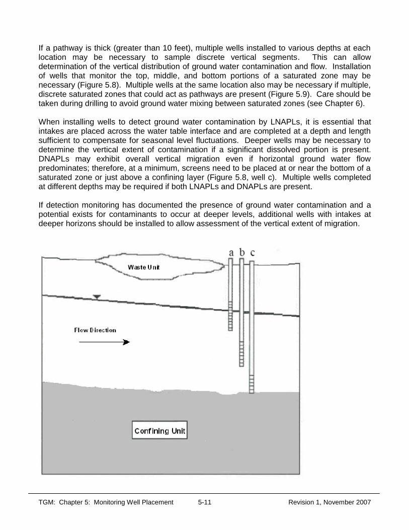
TGM: Chapter 5: Monitoring Well Placement 5-11 Revision 1, November 2007
If a pathway is thick (greater than 10 feet), multiple wells installed to various depths at each location may be necessary to sample discrete vertical segments. This can allow determination of the vertical distribution of ground water contamination and flow. Installation of wells that monitor the top, middle, and bottom portions of a saturated zone may be necessary (Figure 5.8). Multiple wells at the same location also may be necessary if multiple, discrete saturated zones that could act as pathways are present (Figure 5.9). Care should be taken during drilling to avoid ground water mixing between saturated zones (see Chapter 6). When installing wells to detect ground water contamination by LNAPLs, it is essential that intakes are placed across the water table interface and are completed at a depth and length sufficient to compensate for seasonal level fluctuations. Deeper wells may be necessary to determine the vertical extent of contamination if a significant dissolved portion is present. DNAPLs may exhibit overall vertical migration even if horizontal ground water flow predominates; therefore, at a minimum, screens need to be placed at or near the bottom of a saturated zone or just above a confining layer (Figure 5.8, well c). Multiple wells completed at different depths may be required if both LNAPLs and DNAPLs are present. If detection monitoring has documented the presence of ground water contamination and a potential exists for contaminants to occur at deeper levels, additional wells with intakes at deeper horizons should be installed to allow assessment of the vertical extent of migration.

TGM: Chapter 5: Monitoring Well Placement 5-12 Revision 1, November 2007
Figure 5.8. Cluster of wells due to thickness of the saturated unit.
Figure 5.9. Cross-section showing a well cluster.
Length of Intakes In general, intakes should not exceed ten feet; however, the complexity of hydrogeologic conditions or the intended use of wells may dictate that longer (or shorter) intakes are necessary. For example, variable formations necessitate shorter intakes that allow discrete portions to be sampled. If an intake crosses through several alternating zones of high and low K, each zone contributes a different volumetric flow to the total yield. If only one zone is
TGM: Chapter 5: Monitoring Well Placement 5-13 Revision 1, November 2007
contaminated, a sample obtained from such a well will not be representative of the contaminated zone due to sample dilution. Intakes crossing several zones would also provide inaccurate data for flow direction and rate. Additionally, these wells may act as conduits for contaminant migration. Though intake length may depend on the thickness of the saturated zone, it is not synonymous. Intakes shorter than the saturated thickness may be necessary when monitoring homogeneous zones because the behavior of the contaminant may cause it to be concentrated at a particular depth, and long intakes may dilute samples. Likewise, longer intakes may be necessary if a fluctuating water table occurs and the contaminant of concern is lighter than water and floats on the water table surface.
AREAL PLACEMENT OF DOWNGRADIENT WELLS The areal placement of downgradient monitoring wells should be based on the number and spatial distribution of potential contaminant pathways. The components of areal placement include location relative to the pollution source and spacing. The designer should also consider potential receptors such as water supply wells, springs, and surface waters that are downgradient of the pollution source.
Placement Relative to Pollution Source To identify proper locations for ground water sampling, the direction of ground water flow should be determined in all potential contaminant migration pathways. Methods for determining flow direction are discussed in Chapter 3. Knowledge of flow direction is necessary to ensure that wells intended to intercept potentially contaminated ground water are placed hydraulically downgradient of the potential source. To determine if a release has occurred, the downgradient wells should be located laterally along the edge of, or as close as practicable to, the source and have intakes placed to intersect likely pathways. Placing wells through waste management units should be avoided; however, this is sometimes necessary to determine if contaminants are present. In this case, special well construction procedures must be followed to prevent downward movement of waste constituents. In addition, Ohio Revised Code section 3734.02(H) requires authorization from the Director of the Ohio EPA to engage in filling, grading, excavating, building, drilling, or mining on land where a hazardous or solid waste facility has been operated. Mounding may occur where a potential source is topographically higher than the surrounding landscape or where a surface impoundment is in an area where there is a shallow water table. In these situations, it may be necessary to place downgradient wells entirely around the source. Where a potential exists for a DNAPL to sink vertically and accumulate at the interface of a lower impermeable boundary, it may be necessary to place wells that are not downgradient of the pollution source to monitor migrating DNAPL. The dense fluid moves in response to gravity and/or the dip of confining layers and, therefore, may migrate in a direction that is different from the ground water flow direction (Figure 5.10). Knowledge of the slope of the confining layer may be needed to locate and monitor the dense phase. Note that if a dense phase is also soluble in water, a dissolved plume will form and move in the direction of

TGM: Chapter 5: Monitoring Well Placement 5-14 Revision 1, November 2007
ground water flow (Aller et al., 1991). If a DNAPL is soluble, then a detection monitoring system may only need to enable a comparison of downgradient and background ground water samples. If detection monitoring has documented contamination, additional wells should be added at increasing distances away from the source area. The wells should be sampled to assess the horizontal extent of contamination.
Figure 5.10.Migration of a DNAPL along the dip of a confining layer (modified from U.S. EPA, 1993a).
Spacing Spacing refers to the distance between adjacent wells that monitor the same zone. Generally, more complex hydrogeology requires tighter spacing. Monitored zones that exhibit horizontal heterogeneity in material type may necessitate closer or variable spacing. Close spacing may be necessary when a pollution source is underlain by gravelly sand because of the greater potential for rapidly moving, narrow plumes to form. Conversely, zones characterized by low K and high diffusivities (such as a clay-silt) develop wider plumes and larger spacing may be sufficient. Other characteristics that may require wells to be closely spaced include location in or near recharge zones, steep or variable hydraulic gradients, high flow velocity, and variable flow direction.

TGM: Chapter 5: Monitoring Well Placement 5-15 Revision 1, November 2007
Placement of wells in fractured bedrock or bedrock containing solution channels may be difficult. Fractured rock contains numerous zones that may act as discrete pathways for contaminant migration. Monitoring wells often must intersect these zones to be able to provide water or detect contaminants (Chapter 3 addresses methods to locate fractures). Close spacing of wells may be warranted if characterizing leaks of synthetic liners. Such leaks may result in a narrower plume than leaks from an unlined pond. Also, closer spacing may be necessary in areas that are characterized by buried pipes, utility lines, or trenches where point source leaks may occur.
BACKGROUND MONITORING WELL(S) PLACEMENT Background monitoring wells generally are placed hydraulically upgradient of the pollution source. The wells should provide samples that are unaffected by facility operations and representative of background ground water quality. Sampling should be sufficient to account for hydrogeologic heterogeneity and seasonal, temporal, and spatial changes in background water quality. Upgradient or cross-gradient wells may also serve to indicate unanticipated effects of a remedy (e.g., radial flow due to injection of water). Background wells may also be useful in providing a continuous check on the quality of the regional flow system, thus providing early warning of any new contaminants being transported into the remediation area (Gorelick et al., 1993).
Location Background wells are completed in the same stratigraphic horizons as downgradient wells to allow for representative comparisons. Intake length should be selected using the same criteria described earlier in this chapter for downgradient wells. It is also important to locate background wells at a distance from the potential pollution source greater than the radii of hydraulic influence so that the wells will not receive contaminants during development or purging. It may not always be possible or desirable to locate background wells hydraulically upgradient from the source. Situations that may affect the location of background wells include:
Waste sources that are topographically higher than the surrounding landscape may be characterized by radial flow away from the source due to mounding. Surface impoundments located in an area of shallow ground water also may cause mounding.
In some instances, the unit being monitored downgradient may pinch out in the
upgradient direction.
If other activities have affected ground water quality upgradient of the pollution source, the contamination may bias the quality comparison.
Flow direction can vary seasonally or in response to the influence of nearby surface
water or ground water pumping. Due to the changes, no location is clearly upgradient under all conditions.

TGM: Chapter 5: Monitoring Well Placement 5-16 Revision 1, November 2007
The pollution source is situated adjacent to the facility property boundary such that the
upgradient flow direction would dictate a background well to be located off-property.
Upgradient locations are inaccessible due to an obstacle (e.g., other pollution sources, buildings, utilities, etc.).
In these situations, background wells do not need to be upgradient as long as it is demonstrated that 1) they are situated beyond the influence of the pollution source, 2) they are completed in the same zone as the downgradient wells, and 3) the samples provided are representative of background ground water quality. In the case of radial flow, the background wells should be located in an area considered upgradient of the predisposal flow trends.
Number Dependent upon the complexity of hydrogeologic conditions and the number, location, and size of the pollution source, more than one background well may be necessary. Some general situations that may warrant more are as follows:
The pollution source is very large. Multiple potential pollution sources are present. The hydrogeologic setting is characterized by distinctly different hydraulic zones. Background ground water quality varies spatially or seasonally.

TGM: Chapter 5: Monitoring Well Placement 5-17 Revision 1, November 2007
REFERENCES Aller, L., T. W. Bennett, G. Hackett, R. Petty, J. H. Lehr, H. Sedoris, D. M. Nielsen, J. E.
Denne 1991. Handbook of Suggested Practices for the Design and Installation of Ground Water Monitoring Wells. Environmental Monitoring Systems Laboratory, Office of Research and Development, U.S. Environmental Protection Agency. Las Vegas, Nevada. EPA 600/4-89/034. (In cooperation with the National Water Well Association, Dublin, Ohio).
Barcelona, M. J., J. P. Gibb, J. A. Helfrich and E. E. Garske. 1985. Section 2: Essential
Elements of a Ground-Water Sampling Program. Illinois State Water Survey. Illinois State Water Survey, Contract Report 374. pp. 13-33.
Brown, K.W. 1988. Review and Evaluation of the Influence of Chemicals on the Conductivity
of Clay Soils. U.S. EPA, Hazardous Waste Engineering Research Library, Cincinnati, Ohio. EPA/600/52-88/016.
Domenico, P.A. and F.W. Schwartz. 1998. Second Edition. Physical and Chemical
Hydrogeology. John Wiley and Sons. New York, N.Y. Enfield, C.G. and Bengtsson, 1994. Macromolecular Transport of Hydrophobic contaminants
in Aqueous Environments. Ground Water, Vol. 26, No. 1, pp. 64-70. Fetter, C.W. 2001. Fourth Edition. Applied Hydrogeology. Prentice-Hall Englewood Cliffs,
New Jersey. 598pp. Fetter, C.W. 1999. Contaminant Hydrogeology. Macmillan Publishing Company. New York,
NY Freeze, R.A. and J.A. Cherry. 1979. Ground Water. Prentice-Hall Inc. Englewood Cliffs,
N.J. Gorelick, S.M., R.A. Freeze, D. Donhue, and J.F. Keely. 1993. Ground Water
Contamination, Optimal Capture and Containment. Lewis Publishing, CRC Press. Boca Raton, Florida. 385p.
Huling, S.G. and J.W. Weaver 1991. Dense Nonaqueous Phase Liquids. U.S. EPA, Office
of Research and Development, Office of Solid Waste and Emergency Response. EPA/540/4-91-002.
Luckner, L. and M. Schestakow. 1991. Migration Process in the Soil and Groundwater
Zone. Lewis Publishers. Chelsea, Michigan. McCarthy, J.F., 1990. The Mobility of Colloidal Particles in the Subsurface. Hazardous
Materials Control. July/August, pp. 38-43.

TGM: Chapter 5: Monitoring Well Placement 5-18 Revision 1, November 2007
Schwille, F. 1988. Dense Chlorinated Solvents in Porous and Fractured Media; Model Experiments (English Translation). Lewis Publishers. Chelsea Michigan.
Schwille, F. 1981. Groundwater Pollution in Porous Media by Fluids Immiscible with Water.
The Science of the Total Environment. Vol. 21. pp. 173-185 U.S. EPA. 1993, Seminar on Characterizing and Remediating Dense Nonaqueous Phase
Liquids at Hazardous Waste Sites. Office of Research and Development. EPA/600/K-93/003. Cincinnati, Ohio.
U.S. EPA. 1993a. Waste Management Area (WMA) and Supplemental Well (SPW)
Guidance. Office of Solid Waste. Washington, D.C. U.S. EPA. 1992. Corrective Action Glossary. Office of Solid Waste and Emergency
Response. Office of Waste Programs Enforcement. EPA 9902.3-1a. Washington, D.C. U.S. EPA. 1986. RCRA Ground-Water Monitoring Technical Enforcement Guidance
Document. Office of Waste Program Enforcement. Office of Solid Waste and Emergency Response. OSWER-9950.1. Washington D.C.

State of Ohio Environmental Protection Agency
Division of Drinking and Ground Waters
Technical Guidance Manual for Ground Water Investigations Chapter 6
Drilling and Subsurface Sampling
April 2007 Governor : Ted Strickland Director : Chris Korleski
TECHNICAL GUIDANCE MANUAL FOR
GROUND WATER INVESTIGATIONS
CHAPTER 6
Drilling and Subsurface Sampling
April, 2007 Revision 1
Ohio Environmental Protection Agency Division of Drinking and Ground Waters
P.O. Box 1049 50 W. Town Street, Suite 700 Columbus, Ohio 43216-1049
Phone: 614-644-2752 http://www.epa.state.oh.us/ddagw/

TGM Chapter 6: Drilling and Subsurface Sampling 6-ii Revision 1, April 2007
PREFACE
This document is part of a series of chapters incorporated in Ohio EPA’s Technical Guidance Manual for Hydrogeologic Investigations and Ground Water Monitoring (TGM), which was originally published in 1995. DDAGW now maintains this technical guidance as a series of chapters rather than as an individual manual. The chapters can be obtained at http://www.epa.state.oh.us/ddagw/tgmweb.aspx The TGM identifies technical considerations for performing hydrogeologic investigations and ground water monitoring at potential or known ground water pollution sources. The purpose is to enhance consistency within the Agency and inform the regulated community of the Agency’s technical recommendations and the basis for them. In Ohio, the authority over pollution sources is shared among various Ohio EPA divisions, including the Emergency and Remedial Response (DERR), Hazardous Waste Management (DHWM), Solid and Infectious Waste (DSIWM), and Surface Water (DSW), as well as other state and local agencies. DDAGW provides technical support to these divisions. Ohio EPA utilizes guidance to aid regulators and the regulated community in meeting laws, rules, regulations and policy. Guidance outlines recommended practices and explains their rationale. The Agency may not require an entity to follow methods recommended by this or any other guidance document. It may, however, require an entity to demonstrate that an alternate method produces data and information that meet the pertinent requirements. The procedures used to meet requirements usually should be tailored to the specific needs and circumstances of the individual site, project, and applicable regulatory program, and should not comprise a rigid step-by-step approach that is utilized in all situations.

TGM Chapter 6: Drilling and Subsurface Sampling 6-iii Revision 1, April 2007
Major Changes from the February 1995 TGM
The Ohio EPA Technical Guidance Manual for Hydrogeologic Investigations and Ground Water Monitoring (TGM) was finalized in 1995. This guidance document represents an update to Chapter 6 (Drilling and Subsurface Sampling). Listed below are the major changes from the 1995 version. 1. Expanded text for clarity and updated information. 2. Added information on solid-barrel samplers. 3. Added information on the potential for core losses when using coring methods. 4. Removed information on sample storage and preservation for chemical analysis. 5. Modified the decontamination process. This included removing the reference to
using ASTM Type II water for decontaminating equipment. 6. Included references to new documents that has become available since 1995
version, including:
Updated existing references.
Added new ASTM reference for selection of drilling methods for environmental site characterization.
Added reference to the federal Field Sampling and Analysis Technologies Matrix and Reference Guide.
Added reference to the State Coordinating Committee on Ground Water Technical Guidance for Well Construction and Ground Water Protection.
TGM Chapter 6: Drilling and Subsurface Sampling 6-iv Revision 1, April 2007
TABLE OF CONTENTS
PREFACE .................................................................................................................... 6-ii Major Changes from the February 1995 TGM ..............................................................6-iii TABLE OF CONTENTS .............................................................................................. 6-iv FACTORS AFFECTING CHOICE OF DRILLING METHOD ........................................ 6-1
HYDROGEOLOGIC CONDITIONS ........................................................................... 6-1 CONTAMINANT TYPE AND PRESENCE ................................................................ 6-2 NATURE AND SCOPE OF INVESTIGATION ........................................................... 6-3 OTHER FACTORS .................................................................................................... 6-3
DRILLING METHODS .................................................................................................. 6-3 HOLLOW-STEM AUGER ............................................................................................. 4 CABLE TOOL ............................................................................................................... 7 DIRECT ROTARY ........................................................................................................ 7
Water Rotary ............................................................................................................. 8 Air Rotary .................................................................................................................. 8 Air Rotary with Casing Driver .................................................................................. 10 Mud Rotary .............................................................................................................. 11 Dual-Wall Reverse Circulation ................................................................................ 11
RESONANT SONIC ................................................................................................... 12 OTHER METHODS .................................................................................................... 14 GENERAL RECOMMENDATIONS ............................................................................ 16
SAMPLING SUBSURFACE SOLIDS ............................................................................ 17 Solid-Barrel Samplers ............................................................................................. 18 Split-Barrel Sampler ................................................................................................ 18 Thin-wall Sampler .................................................................................................... 18 Vicksburg and Dennison Samplers ......................................................................... 22 Piston Samplers ...................................................................................................... 22 Continuous Sampling Tube ..................................................................................... 25 Core Barrel .............................................................................................................. 25
IMPLEMENTATION ................................................................................................... 26 Common Field Problems ......................................................................................... 26 Sampling Interval..................................................................................................... 27 Sample Storage and Preservation........................................................................... 27 Data Requirements ................................................................................................. 28
DECONTAMINATION ................................................................................................ 28 Decontamination Area ............................................................................................. 28 Typical Equipment Requiring Decontamination/Disposal ........................................ 29 Frequency ............................................................................................................... 29 Procedures and Cleaning Solutions ........................................................................ 29 Quality Control Measures ........................................................................................ 30
INVESTIGATION BY-PRODUCTS, CONTAINMENT AND DISPOSAL ..................... 30 CONTROL AND SAMPLING OF ADDED FLUIDS ..................................................... 32 PERSONNEL SAFETY .............................................................................................. 32
REFERENCES .............................................................................................................. 33

TGM Chapter 6: Drilling and Subsurface Sampling 6-1 Revision 1, April 2007
CHAPTER 6 DRILLING AND SUBSURFACE SAMPLING
Drilling and sampling of boreholes represent important components of virtually all ground water investigations. Drilling should minimize disturbance of the subsurface. Methods should identify saturated zones and sample formation materials to characterize the subsurface and, subsequently, allow for proper monitoring well installation. Appropriate quality assurance/quality control (QA/QC) procedures, including equipment decontamination and measures to prevent cross-contamination of subsurface zones, should be implemented. The following sections discuss drilling, subsurface sampling, and QA/QC.
FACTORS AFFECTING CHOICE OF DRILLING METHOD The choice of drilling method should be based on expected performance when hydrogeologic conditions, contaminant type and presence, and the nature and scope of the investigation are considered. Additional factors include site access and equipment availability. HYDROGEOLOGIC CONDITIONS For most sites, hydrogeology is the most important factor in drilling method selection. If work is just beginning, initial literature and data searches for the surrounding area should be conducted to obtain a general knowledge of the local geology and the occurrence of ground water. If borings have been performed on or near the site, available logs may prove valuable. Hydrogeologic conditions affecting the choice of methods include: • Material Consolidation: Some methods can penetrate unconsolidated
materials, but not rock.
• Material Cohesiveness: When drilling through cohesive material, an open borehole can be maintained and a well can be installed directly. However, when penetrating less stable and collapsing formations, the method should allow casing or the drill string to be used to maintain the borehole.
• Thickness of Formation: If thin, intermittent sand lenses are of interest,
methods offer differing capabilities of allowing their identification. Most, however, can detect a thick, high-yield zone.
• Presence of Fractures: Fractures in rock and porous, unconsolidated material
may cause lost circulation of fluids and hinder penetration. Where this is a problem, casing may have to be advanced closely behind the bit. Therefore the
chosen method should permit casing installation during drilling (Davis et al., 1991).

TGM Chapter 6: Drilling and Subsurface Sampling 6-2 Revision 1, April 2007
• Presence of Cobbles and Boulders: The presence of cobbles and boulders can hinder advancement of a bit. Where cobbles and boulders are present, a method should be chosen that can penetrate the materials effectively.
• Heaving Sands: Some equipment may be limited in its ability to drill below the
water table, particularly in loose granular soils. With some methods, sand or gravel can flow into the drill stem, making sample retrieval and well installation difficult. Special equipment may be needed.
Aller et al. (1991) developed a rating system to determine applicable drilling methods for various generic geologic situations. The Federal Remediation Technologies Roundtable has produced a simpler matrix of drilling methods that is available at http://www.frtr.gov/site/samplegif.html). Methods were rated for versatility, sample reliability, relative cost, availability, relative time required for well installation and development, ability to preserve natural conditions, ability to install particular well diameters, and relative ease of well completion and development. This system can help narrow the choices to those most applicable to site conditions. CONTAMINANT TYPE AND PRESENCE Characteristics of contamination that can affect the choice of drilling method include:
• Contaminant Phase: If contaminants are present in the gaseous phase, the method should contain the contaminants, minimize losses to the atmosphere, and reduce any explosive potential. If free product is present, methods should be utilized to detect it. In certain situations, type and amount of contamination can be anticipated.
• Potential for Cross-Contamination: To monitor a zone of unknown ground
water quality that underlies a contaminated zone, adequate precautions should be taken to prevent cross-contamination. Generally, the portion of the borehole opposite an upper water-bearing zone should be drilled, cased, and grouted separately. A smaller diameter borehole then should be completed through the grouted casing into the underlying zone. This process, often referred to as "telescoping", and should prevent migration of contaminants from the upper zone into the lower zone. Hackett (1987) provided specific details for this technique when hollow-stem augers are used.
• Concentration of Contaminants: Where high concentrations of contaminants
are present, extra precautions for equipment decontamination and disposal of fluids (if used) and cuttings should be considered. Fluid and cuttings may need to be disposed as hazardous waste. Thus, waste minimization may be a major concern for method selection.
TGM Chapter 6: Drilling and Subsurface Sampling 6-3 Revision 1, April 2007
NATURE AND SCOPE OF INVESTIGATION The drilling method should allow for identification of subsurface geology and water-producing zones based on the nature and scope of the investigation. Factors that can dictate method selection include:
• Monitoring Well Depth and Diameter: The method must be able to meet the depth and diameter requirements of proposed monitoring wells. Casing typically ranges from two to four inches in diameter. Wells that will be pumped for tests or remediation may need to be at least 4 inches in diameter to allow access for pumps and to provide adequate yield. Sufficient space must be present in boreholes to allow adequate installation of seals and filter packs, unless pre-packed well screens are used with small diameter wells (see Chapter 15 - Use of Direct Push Technologies for Soil and Ground Water Sampling).
• Knowledge of Site Hydrogeology: If little or no background information is
available, it may be desirable to perform a small scale hydraulic test on selected zones or sample ground water for contaminant analysis. The ability to collect samples during drilling varies according to the method used and the ability to pump the zone of interest. In some cases, a screened drill string may be employed. In other cases, a well point or in-situ sampler (e.g., DPT sampler, see Chapter 15 - Use of Direct Push Technologies for Soil and Ground Water Sampling) can be driven ahead of the borehole base. The driven tool is then pumped to remove fine sediment and provide a sample. After sampling, the device is retrieved and drilling is resumed. These tools may be used with any method that allows easy access to the borehole bottom. However, they should only be used as a screening tool. A well point should not be used as a permanent monitoring well.
OTHER FACTORS Physical features alone potentially can influence the choice of drilling method. Moving large equipment over rough or muddy terrain or into tight spaces between physical obstructions may be required. Rig movement can be hindered by overhead powerlines or structures common around industrial areas. Regional geology and demand play a major role in determining equipment availability, which is another factor.
DRILLING METHODS The following discussion provides a general description of recommended drilling methods for monitoring well installation. These include hollow-stem auger, cable tool, and rotary techniques. Again, site conditions should dictate the selection. One (or a combination) should be adequate to satisfy most situations.

TGM Chapter 6: Drilling and Subsurface Sampling 6-4 Revision 1, April 2007
HOLLOW-STEM AUGER Hollow-stem augers are readily available in Ohio, and are recommended for penetrating unconsolidated materials. Auger rigs are light and maneuverable. Each section or flight is typically 5 feet in length. A head is attached to the first flight and cuttings are rotated to the surface as the borehole is advanced (Figure 6.1). A pilot bit (or center bit) can be held at the base of the first flight with drill rods to prevent cuttings from entering. When the bit is removed, formation samples can be obtained through the auger using split-spoon or thin-wall samplers. Generally, fluids do not need to be introduced; therefore, ground water quality alteration usually is avoided. Hackett (1987, 1988) has reviewed procedures for using hollow-stem augers. ASTM D 5784-95 (reapproved 2000) also provides guidance. One of the major advantages of hollow-stem augers is that they allow for well installation directly through the auger into non-cohesive material. Table 6.1 shows auger sizes typically available. The inside diameter of the hollow-stem is generally used to specify size, not the diameter of the hole drilled. Appropriate clearance should be available to provide effective space for materials placement. The augers are removed as the well is installed (SCCGW, 2000). If space is insufficient, bridging of the materials may bind the casing and auger together, resulting in the extraction of the well as the auger is removed (Hackett, 1988). Additionally, insertion of a tremie pipe may be difficult. The most widely available size is 3.25-inch (6.25-inch outside diameter, including the flights), which has been used to install 2-inch (2.378 outside diameter) monitoring wells; however, this allows limited access. It is doubtful that materials can be placed adequately at depths below 15 feet considering the relatively small amount of clearance offered. The minimum size that should be used for installation of 2-inch diameter casing is 4.25 inches; however, larger augers may be necessary. The depth capability of hollow-stem augering depends on site geology and the size of the rig and stem. In general, greater depths can be reached when penetrating clays than when penetrating sands; however, clays may cause the auger to bind, which limits depths. The size of the rig and stem affects the downward pressure and torque on the stem. Greater depths may be reached by smaller augers. Depths of 200 + feet can be reached utilizing a 4.25-inch hollow-stem auger, whereas 10.25-inch augers can reach a maximum depth of approximately 75 feet. Hollow-stem augering presents some disadvantages. It cannot penetrate cobbles and boulders nor most rock formations. In some cases, obstructions can be pushed aside by spinning the augers in-place. When this is not successful, replacing the pilot assembly with a small tri-cone bit may allow penetration. Additionally, carbide-tipped cutting teeth have been developed for the upper portions of weathered bedrock, which may be useful when the unconsolidated/bedrock interface is the zone of interest.
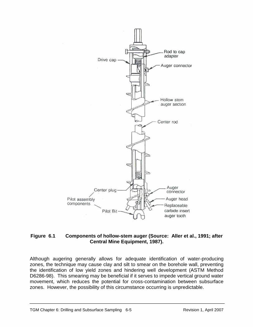
TGM Chapter 6: Drilling and Subsurface Sampling 6-5 Revision 1, April 2007
Figure 6.1 Components of hollow-stem auger (Source: Aller et al., 1991; after
Central Mine Equipment, 1987). Although augering generally allows for adequate identification of water-producing zones, the technique may cause clay and silt to smear on the borehole wall, preventing the identification of low yield zones and hindering well development (ASTM Method D6286-98). This smearing may be beneficial if it serves to impede vertical ground water movement, which reduces the potential for cross-contamination between subsurface zones. However, the possibility of this circumstance occurring is unpredictable.

TGM Chapter 6: Drilling and Subsurface Sampling 6-6 Revision 1, April 2007
Table 6.1 Typical auger sizes available for monitoring well drilling (Central Mine Equipment, 2006).
STANDARD SIZE HOLLOW-STEM AUGER (Central Mine Equipment Company, 2006)
Hollow-Stem Inside Diameter (inches)
Flighting Diameter (inches)*
Auger Head Cutting Diameter (inches)
2 1/4 2 3/4 3 1/4 3 3/4 4 1/4 6 1/4 8 1/4
5 5/8 6 1/8 6 5/8 7 1/8 7 5/8 9 5/8 12 1/4
6 1/4 6 3/4 7 1/4 7 3/4 8 1/4 10 1/2 13
*NOTE: Auger flighting diameters should be considered minimum manufacturing dimensions.
The use of hollow-stem augers may be hindered by "heaving sands," which occur when a confined, saturated sand unit is encountered. Infiltration of the sand and water into the augers causes them to bind. Common strategies to alleviate this include (Aller et al., 1991):
• Water may be added to maintain a positive downward pressure to offset the pressure of the formation.
• Drilling muds can be added to further offset the pressure.
• The lower portion of the auger may be perforated to allow formation water to
enter. This will equalize the hydraulic pressure and prevent entrance of sediments. Screened augers (Taylor and Serafini, 1988) have been developed for this purpose, although strength and structural integrity is lost.
• The pilot bit can be kept in place or a knock-out plug or winged clam can be
added to the base of the hollow-stem to prevent infiltration. The most common approach is to add water to the hollow-stem (Aller et al., 1991). If this is done, only clean, potable water of known chemical quality should be used. Drilling muds are not recommended because the quality of water samples and the integrity of the formation matrix may be affected. Screened augers may be viable. The pilot bit, knock-out plug or winged clam may not be useful when formation samples are needed because the removal of these devices to sample will result in the entrance of sand. The knock-out plug may be useful if prior site characterization eliminates the need for the collection of formation samples.
TGM Chapter 6: Drilling and Subsurface Sampling 6-7 Revision 1, April 2007
CABLE TOOL The cable tool is the oldest drilling method and is readily available throughout Ohio. A heavy string is dropped repeatedly to penetrate the subsurface. The bit crushes rock and causes loosening and mixing in unconsolidated formations (Driscoll, 1986). When penetrating unconsolidated materials, outer casing must follow the bit closely as the boring is advanced to prevent caving. The outer casing often is driven ahead of the hole bottom to prevent cross-contamination (ASTM Method D6286-98). The cuttings are removed periodically with a bailer. Cable tools drill a wide variety of hole diameters to almost unlimited depths. Individual water-bearing zones and changes in formation often are more easily identified with cable tool drilling than with other methods (e.g., smearing along sidewalls generally is less severe and thinner than with hollow-stem augering). Representative samples can be collected by driving tools (e.g., split-spoon) ahead of the hole bottom. Well installation and development are relatively easy when this drilling method is used. Additionally, the method typically produces a low volume of fluids and cuttings that need disposal (Davis et al., 1991). Cable tool does have some disadvantages. The rate of penetration is very slow, with rates of 10 to 20 feet per day common (Davis et al., 1991). Problems with "heaving" sands are possible, just as with the hollow-stem auger. When drilling through unsaturated materials, water must be added to form a slurry so cuttings can be bailed. Finally, the driven outer steel casing is not adequate for monitoring well design. The undesirable effects of the presence of the steel casing can be avoided by installing an inner casing of the proper composition. The driven casing is retracted by driving it upward or raising it with hydraulic jacks; however, it may be difficult to remove long strings without special equipment. For most site conditions and investigative goals, cable tool is an acceptable alternative to hollow-stem augering. Its ability to penetrate both rock and unconsolidated formations with the limited introduction of fluids make it an excellent option. In general, cable tool drilling is recommended for installation of large diameter wells (6-10 inch well casing) to all depths in unconsolidated and unsaturated conditions. It also is an adequate substitute to hollow-stem augering where hollow-stem augering is not feasible (i.e., deep wells in unconsolidated formations, or drilling through cobbles and boulders). However, the rate of drilling can be slow, which may limit the feasibility of cable tool. DIRECT ROTARY Direct rotary drilling is known for the speed at which it penetrates. A bit is rotated against the sides of the borehole. Circulation of fluids (i.e., water, mud, or air) (Figure 6.2) lubricates and cools the bit, removes cuttings, and maintains and seals the borehole wall. The fluid and cuttings return to the surface between the drill pipe and borehole wall.
TGM Chapter 6: Drilling and Subsurface Sampling 6-8 Revision 1, April 2007
One of two methods are used to rotate the drill bit: a table drive or a top head drive. The rotating motion of the table or top head is transferred to the drill rods, which rotate the bit (SCCGW, 2000). Several types of bits may be utilized, including drag, roller cone, and tricone. Drag bits are used to penetrate unconsolidated and semi-consolidated deposits. Roller cone bits are preferred when drilling through consolidated rock. Tricone bits are effective for every type of formation (Driscoll, 1986). In-situ samples may be taken by using a bit with an opening through which sampling tools can fit. However, circulation must be broken to collect samples. Though samples can be obtained directly from the stream of circulated fluid by placing a collection device in the discharge flow, their quantity is insufficient. Water Rotary Water rotary is effective for penetrating most hydrogeologic environments (U.S. EPA, 1992). It can readily penetrate both soil and rock to essentially unlimited depths (ASTM Method D6286-98). However, it is recommended only where the water will have limited effects on the formation matrix and ground water chemistry. Clean, potable water of known chemical quality transported from off-site should be used. This method works best when penetrating rock formations where a stable borehole can be maintained. Use of water rotary is limited because the water may mix and/or react with formation water and hamper the identification of water bearing zones. In addition, the water cannot maintain the borehole wall or prevent the in-flow of fluids from unconsolidated formations, nor can it prevent cross-contamination. It may be desirable to drive casing during drilling. Another option is to complete a multiple-cased well where each section is grouted and successively smaller diameter holes and casing are completed. Heaving sands may cause a problem unless proper pressure can be maintained in the borehole water column. Air Rotary Air rotary involves forcing air down the drill string to cool the bit and remove cuttings through the annulus (Aller et al., 1991). No muds are used that "cake" onto the borehole wall, although water and/or foams often are added to improve penetration rates (foam should not be used because it can affect the borehole chemistry (ASTM Method D6286-98). Air removes cuttings effectively and maintains a clean borehole wall, thus allowing for a greater ease in well completion and development. This method can provide a wide range of borehole diameters and is readily available throughout Ohio.

TGM Chapter 6: Drilling and Subsurface Sampling 6-9 Revision 1, April 2007
Figure 6.2 Diagram of a direct rotary circulation system(Source: Aller et al, 1991; after National Water Well Association of Australia, 1984).
Air rotary is best justified for penetrating rock (competent or fractured). The depth of drilling is unlimited for all practical purposes (ASTM Method D6286-98). Its use in unconsolidated formations is limited due to potential borehole instability. Overburden casing is commonly necessary (ASTM Method D6286-98). Hollow-stem augers are often used to drill through the unconsolidated deposits, while air rotary is used to complete boreholes into the bedrock. The identification of thick water-bearing zones is relatively easy, but the identification of thin zones within dry formations can be difficult due to the pressure of the air, its drying effects, and sorption of moisture by the cuttings. Where thin zones are anticipated, drilling should be slowed or stopped to allow any ground water to enter the borehole. This method will work only for the uppermost zones because shallow infiltration hinders the detection of lower zones. Increased grain size of cuttings also may aid in the identification of water-bearing zones as the size of cuttings, typically fine-grained, increases once water is encountered or added.
TGM Chapter 6: Drilling and Subsurface Sampling 6-10 Revision 1, April 2007
A disadvantage of air rotary is that compressors often introduce hydrocarbon-related contaminants to the borehole. As a result, in-line filters should be installed and checked regularly for clogging. Conversely, the air stream can potentially strip volatile contaminants from the borehole wall. In addition, control and containment of cuttings at contaminated sites may be difficult. Added safety precautions should be considered due to the abundance of dust, mists and potential volatilization of organic compounds. Down-hole hammer bits often are substituted for the roller cone bit for a percussion effect to speed penetration through very hard rock (Aller et al., 1991), boulders, and cobbles. A pneumatic drill hammers the rock while the bit is slowly rotated (ASTM Method D6286-98). However, because oil is required in the air stream to lubricate the hammer bit, this technique is not recommended. The potential for cross-contamination is great due to the lack of casing to seal off specific zones. Therefore, air rotary techniques should not be used when upper layers are contaminated. Another concern is the effect on formation geochemistry and water quality due to the introduction of air. Air can change redox state and also may enhance biodegradation and volatilization. Through time and proper well development, these effects eventually may disappear. It is important that knowledge of the local geochemistry and potential contaminants be obtained and weighed into the determination of whether the method is appropriate. Air Rotary with Casing Driver A casing driver can be used with air rotary as the bit advances. This allows unconsolidated formations to be penetrated because the driven casing prevents borehole collapse (Aller et al., 1991). Moreover, the casing seals off contaminated water-bearing zones and can prevent cross-contamination (ASTM Method D6286-98). Normally, the bit is advanced 6 to 12 inches ahead of the casing. It also is possible to advance the casing ahead of the bit and use the drill to clean out the casing. This technique may be necessary for caving and slumping formations and can minimize air contact with the formation. Air rotary with a casing driver is most applicable for penetrating unconsolidated formations where gravel and boulders exist and air introduction is acceptable. It also may be useful for drilling through unconsolidated formations to depths that the hollow-stem auger cannot attain, although increased friction may hinder penetration below 200 feet in dry, unconsolidated materials (Davis et al, 1991). Telescoped boreholes and casing may help overcome this problem. Air rotary with a casing driver can be used when both rock and unconsolidated formations must be penetrated. The driver is used to complete a cased borehole through the unconsolidated materials and strict air rotary methods are used once rock is encountered. When completing a monitoring well, the surface casing can be driven upward to expose the well intake once the screen and casing have been installed. The filter pack and annular seal are installed as the driven casing is retracted. Woessner (1987) provided additional information on the air rotary with casing driver method.
TGM Chapter 6: Drilling and Subsurface Sampling 6-11 Revision 1, April 2007
Air rotary with casing driver has several disadvantages. The equipment is expensive and not readily available. Extracting the casing can damage the well screen (ASTM Method D6286-98). Mud Rotary Mud rotary is common in the oil and water well industry. Typically, bentonite-based mud is added to maintain positive pressure and the borehole walls. The introduction of mud generally "cakes" the formation with fine material that must be extracted during well development. This virtually prevents the identification of water-bearing zones. Also, mud commonly infiltrates and affects water quality by sorbing metals and polar organic compounds (Aller et al., 1991). If organic polymer additives are used, bacteria levels in the formation will increase and cause local biodegradation that may affect organic compound analysis (Aller et al., 1991). Only in rare cases should this method be used. Prior consultation with Ohio EPA is recommended before drilling with mud. Dual-Wall Reverse Circulation Dual-wall reverse circulation rotary involves the circulation of either mud, water, or air between inner and outer casings of the drill string (Aller et al., 1991) (Figure 6.3). The inner casing rotates, acting as the drill pipe, while the outer pipe acts as casing. The fluid is pumped down the outer casing to cool and lubricate the bit. The fluid then returns to the surface with cuttings through the inner casing. The dual wall maximizes the energy at the bit with minimal loss of fluids. The outer casing allows for stabilization of the borehole, prevents caving around the bit, minimizes cross-contamination from cuttings, and allows minimal vertical contaminant migration. This method may not be readily available in most areas of Ohio. It is best suited for deep (>150 ft.) drilling through unconsolidated materials, but it is also efficient for penetrating rock. Dual-wall reverse circulation can drill rapidly to depths exceeding 1000 feet. Wells may be completed in the open hole or through the inner casing. Wells completed in the inner casing are limited to a maximum casing diameter of four inches (Strauss et al., 1989); however, with this size, it is often difficult to install the filter pack and annular seal through the drill string. A variety of fluids are utilized with the dual-wall method. The introduction of mud is not recommended. Only clean, potable water (pre-analyzed with rigid QA/QC) should be used. If air is used, in-line filters are necessary to prevent the introduction of lubricants into the hole. Down-hole air hammer bits often are used with the dual-wall method. As with air rotary, the need for lubricants in the hammer bit makes this tool unacceptable. Strauss et al. (1989) discussed applications of the dual-wall method and a percussion driver system. The driver advances the outer wall pipe by force instead of rotation. As open-faced bit is used that breaks the formation into fragments small enough to pass through the inner casing. These larger samples allow for more accurate determination of formation characteristics than do the pulverized cuttings of the rotary method. Split spoon samplers and Shelby tubes may be inserted through the inner casing and the open-faced bit to sample undisturbed material ahead of the drill string. Penetration rates

TGM Chapter 6: Drilling and Subsurface Sampling 6-12 Revision 1, April 2007
of 60 ft/hr in unconsolidated sediments to depths of 300 to 450 feet are possible. A third outer casing can be driven while the dual-wall string advances. This is called "triple-wall" drilling. The extra casing is used to prevent cross-contamination by sealing off an upper, shallow, contaminated zone when drilling to a lower zone. RESONANT SONIC Sonic drilling, rotasonic, sonicore, vibratory, rotosonic, or resonant sonic drilling all refer to the same technology. The resonant sonic drilling method is a relatively new technique that is being used successfully in Ohio. The method performs most efficiently at depths of 30 to 300 feet. It combines rotation with high frequency vibration to advance a core barrel to a desired depth. The vibration is stopped, the core barrel is retrieved, and the sample is vibrated or hydraulically extracted into plastic sleeves or sample trays (Dustman et al., 1992). This drilling technique vibrates the entire drill string at a frequency between 50 and 150 cycles per second. When the vibrations coincide with the natural frequency of the steel drill rod or casing a natural phenomenon called resonance occurs. Resonance allows the drill rig to transfer the vibrational energy into the top of the drill string, allowing for very fast (up to 1 foot/second in certain formations) penetration rates (Boart Longyear Co.). Monitoring wells can be installed through an outer casing. Continuous, relatively undisturbed samples can be obtained through virtually any formation. Conventional sampling tools can be employed as attachments (i.e., hydropunch, split spoon, shelby tube, etc.). No mud, air, water, or other circulating medium is required. The sonic method can drill easily at any angle through formations such as rock, sand, clay permafrost, or glacial till.

TGM Chapter 6: Drilling and Subsurface Sampling 6-13 Revision 1, April 2007
Figure 6.3 Diagram of the dual-wall reverse circulation method (Source: U.S. Bureau of Reclamation Earth Manual, Part I, 3rd ed.)
TGM Chapter 6: Drilling and Subsurface Sampling 6-14 Revision 1, April 2007
Case histories of projects using the method demonstrate excellent results but indicate several problems (Barrow, 1994). One of the major disadvantages is the limited availability of the rigs and experts to operate them. Current rigs are operated somewhat by feel and by ear. Although numerous gauges monitoring hydraulic pressures are usually present, successful drilling is accomplished because of the skill of the driller. In addition, the equipment is relatively expensive and the cost per foot of penetration is higher than for conventional methods; however, the method has been shown overall to be more cost- and schedule-effective for hazardous waste site characterization (Barrow, 1994). Penetration rates of 15 to 60 feet per hour were cited by Barrow (1994). In addition, the method minimizes the amount of waste by-products generated. The resonant sonic method can create elevated temperatures in samples from certain formations. This is a potential problem when projects are evaluating the occurrence of volatile organic compounds (VOCs) (ASTM Method D6286-98). Another potential problem is that the speed of sample generation may overwhelm the geologist responsible for logging the borehole. In addition, the amount of samples to be tested may be beyond the capacity of a laboratory to analyze on a timely schedule if it is not prepared to handle large quantities. If the project manager recognizes this, he/she can plan for these problems prior to the start of drilling. An additional problem is that the method may destroy soft bedrock (i.e., shales); therefore, sample recovery may be low. OTHER METHODS Several other methods are common in the geotechnical industry, including solid flight augers, jet percussion, reverse circulation, hand augers, and manual driving. While generally not recommended for monitoring well installation, there may be exceptions where these methods may be justified. In these cases (as in all others), the responsible party should document the rationale used for the choice. Solid flight augers function just as hollow-stem augers except that the stem is solid. This prevents the collection of in-situ formation samples. Well installation can be conducted only in stable formations because maintaining an open borehole below the water table after auger removal is often difficult. The hollow-stem auger provides the same function and is more versatile. Therefore, hollow-stem augers are preferred at all times. Reverse circulation is, in principle, the same as the rotary method but with fluids flowing in the opposite direction. The fluid flows down the borehole annulus to the bit and is returned with the cuttings up the drill string. Reverse circulation differs from the dual-wall method due to the lack of an outer casing wall to manage the fluid and prevent its contact with the borehole wall. This method typically is used to drill large diameter boreholes. Jet percussion is used infrequently and involves injecting water under pressure down the drill pipe against a wedge-shaped bit. The drill string is lifted and dropped repeatedly during drilling to loosen the soil (ASTM Method D6286-98). Its use is limited

TGM Chapter 6: Drilling and Subsurface Sampling 6-15 Revision 1, April 2007
to shallow (<150 ft.), unconsolidated deposits with a maximum casing diameter of 4 inches. A hollow-stem auger is the preferred method for these conditions. The injection of fluid, potential for cross-contamination, and limited well diameter restrict the desirability of this method. Jet wash drilling is similar to jet percussion with the exception that the drill bit is not dropped during drilling (ASTM Method D6286-98). Hand augers are most applicable for shallow piezometer and lysimeter installation. They can reach a depth of 15 feet in unconsolidated materials. This method only can be used to penetrate cohesive materials because a stable borehole wall is necessary for well installation. Generally, the borehole cannot be advanced below the water table. Driven well installation involves the insertion of a well point (or screen) and casing into the subsurface by hand driving or with a large weight (Figure 6.4). Well points consist of a well screen with a hardened point on the end of the screen, and are installed only in unconsolidated formations (SCCGW, 2000). Driving the device through fine silts, clays, and boulders is often very difficult. Depths of 50 feet or less are common. Driven wells should not be used as permanent data collection points. As the tool is driven, it tends to smear clays, preventing ground water from entering the screen and, subsequently, hindering well development. The annular space remains unsealed; therefore, the potential for vertical movement of surface water and/or contaminants increases. Furthermore, formation samples cannot be collected, which hinders proper screening and prevents geologic and contaminant characterization. This method has greater application for plume delineation and tracking studies, where reconnaissance investigation can help determine the extent of contamination. In these situations, prior knowledge of subsurface geology, water-bearing zones, and sampling depths is necessary. Properly constructed monitoring wells should be installed to verify the data. Larger volumes of water/mud are needed for this method than for the direct rotary method. The potential for large losses of fluids often is present when drilling through permeable formations. This can cause extensive ground water quality degradation around the borehole.

TGM Chapter 6: Drilling and Subsurface Sampling 6-16 Revision 1, April 2007
Figure 6.4 Diagram of a well point (Source: Aller et al., 1991). GENERAL RECOMMENDATIONS General recommendations can be provided regarding selection of drilling methods and practices for sites in Ohio and the factors that dictate the choice. Experience indicates that geology is the primary factor for most sites. Table 6.2 summarizes the methods that generally apply for various geologic environments. Hollow-stem augering is recommended whenever possible. Resonant sonic is also favored; however, because of its limited availability and application, recommended conventional methods are generally accepted in its place. Shallow wells in the glaciated portions of northern, western and central Ohio usually can be installed with hollow-stem augers, although penetration of deep, sandy materials may not be possible. Drilling through the consolidated materials at the surface of eastern Ohio may require use of cable tool or air rotary techniques. Air rotary with casing driver may be appropriate to retain the upper unconsolidated and weathered materials as the underlying bedrock is penetrated. Hollow-stem augering may be applicable in eastern Ohio to drill through alluvial deposits and unconsolidated and weathered surface deposits overlying bedrock. Cable tool or air rotary methods may be necessary in western Ohio to penetrate the bedrock underlying the unconsolidated shallow glacial deposits. Methods requiring use of fluids (air, water, and mud) should be avoided whenever possible. If fluids are necessary, water and air are more acceptable than mud, which

TGM Chapter 6: Drilling and Subsurface Sampling 6-17 Revision 1, April 2007
can have a long-term effect on ground water quality. Water used should be recovered. All fluids and cuttings should be routed directly to the surface and isolated from contact with the formation. Air rotary with casing driver and the use of air with the dual-wall reverse circulation method provide protection from air infiltration. The use of water for cable tool drilling may be acceptable because it is only necessary while drilling through the unsaturated zone. Table 6.2 Summary of drilling methods recommended for different types of
geologic materials.
GEOLOGIC MATERIALS
DRILLING METHODS
Hollow-Stem
Augers
Cable Tool
Dual-Wall Circulation
Air-Rotary With Casing
Driver
Resonant Sonic Method
Unconsolidated
X X X X X
Consolidated, Fractured and/or Weathered
X X X
Consolidated, Competent
X X X
SAMPLING SUBSURFACE SOLIDS During drilling of a monitoring well borehole, samples of formation material should be collected to help in the selection of filter pack and well screen sizes and aid in the placement of the well intake. Field and laboratory analysis of the samples also can provide information that can be used to prepare geologic cross-sections, identify water-producing zones, and determine contaminant concentrations. Appropriate tools should be used. Cuttings brought to the surface are not suitable as samples because they are pulverized and do not reflect the true nature of the formation. Furthermore, accurate determination of the horizon of the cuttings is often difficult or impossible. SUBSURFACE SAMPLERS Most samplers have been designed to sample ahead of a bit. Types include thin-wall, split-spoon, core barrel, and continuous tube. The tool chosen should provide samples that represent the subsurface environment to the highest degree possible. Selection should be based on site geology, the drilling method, and investigative goals. All of the samplers discussed here are acceptable.

TGM Chapter 6: Drilling and Subsurface Sampling 6-18 Revision 1, April 2007
Solid-Barrel Samplers Solid-barrel samplers are generally steel or stainless steel cylinder generally between 12 and 60 inches in length and between 1 and 6 inches in diameter. They may be used with liners that may be made of brass, stainless steel, or plastic. Solid-barrel samplers are often used with DPT systems and are discussed in Chapter 15 - Use of Direct Push Technologies for Soil and Ground Water Sampling. Split-Barrel Sampler The split-barrel (also called split-spoon) sampler is commonly used for collecting unconsolidated formation samples (Figure 6.5). This tool works efficiently with hollow-stem augers, which allow for sampling directly through the auger and ahead of the bit. It also works efficiently with cable tool but offers limited use with rotary. The sampler is comprised of an 18 to 24 inch long cylinder that splits in half length-wise to yield the cored sample. They are generally available in diameters from 1 to 3.5 inches (Ruda and Farrar, 2006). Samples are collected by lowering the tool to the base of the borehole with drill rods and driving it into the subsurface with a 140 pound weight (or "hammer"). The sampler should be driven about 6 inches less than its length to avoid sample compression. Coarse material sometimes catches in the sampler, preventing complete recovery. To help reduce sample loss, retainers have been designed (Figure 6.6). A complete description of collection of split-spoon samples is contained in ASTM D1586-99 (1994). Split-spoon samples are acceptable for formation identification and characterization. However, they are considered to be "disturbed", due to the relatively large wall thickness of the split-spoon, which causes compaction of the sediment as it enters. Because of this compaction, this tool should not be used when samples are to be submitted for laboratory analysis for physical parameters (such as hydraulic conductivity). Split-spoon samples are acceptable for chemical analysis, however. They are often used in conjunction with liners for ease of sample collection and removal (Ruda and Farrar, 2006). Standard Penetration Tests (ASTM, Method D1586-99) typically are conducted with the split-spoon sampler for a relative indication of formation consolidation. Generally, this involves lifting and dropping a weight across a 30-inch span and recording blow counts ("N") for each 6 inches of advancement. "Sample refusal" occurs when blows exceed 50 with little or no downward progress. The sampling effort can be stopped at this point and drilling may continue (if possible). Thin-wall Sampler The thin-wall sampler is of two types: open (or Shelby Tube) or piston-type. Both are used for collecting undisturbed, in-situ soil samples (Figure 6.7). According to ASTM Method D669-98, an undisturbed sample is collected taking every precaution to minimize sample disturbance. The wide diameter and thin walls of the tube allow for very minimal disturbance. The tube is attached to the drill rods and slowly pushed

TGM Chapter 6: Drilling and Subsurface Sampling 6-19 Revision 1, April 2007
Figure 6.5 Diagram of a split spoon sampler (Source: Aller et al., 1991; after Mobile Drilling Company, 1982).
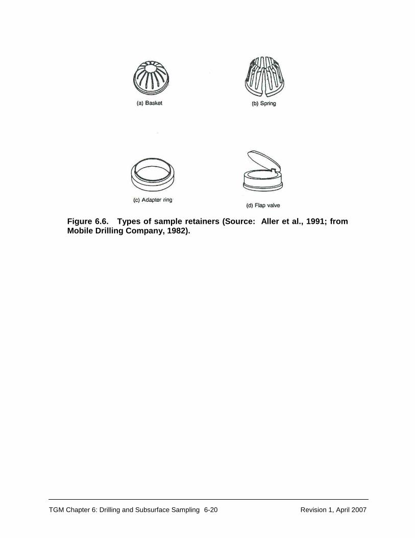
TGM Chapter 6: Drilling and Subsurface Sampling 6-20 Revision 1, April 2007
Figure 6.6. Types of sample retainers (Source: Aller et al., 1991; from Mobile Drilling Company, 1982).
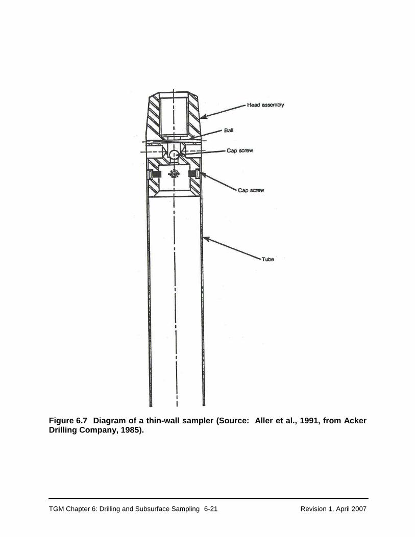
TGM Chapter 6: Drilling and Subsurface Sampling 6-21 Revision 1, April 2007
Figure 6.7 Diagram of a thin-wall sampler (Source: Aller et al., 1991, from Acker Drilling Company, 1985).
TGM Chapter 6: Drilling and Subsurface Sampling 6-22 Revision 1, April 2007
ahead of the existing hole. Upon removal, the tube should be sealed on both ends and transported as an entire unit for analysis (e.g., permeability, moisture content, porosity etc.). The "top" or "up" direction should be marked so that the laboratory will orient the sample correctly. The procedures are described in detail in ASTM Method D1587-00. The thin-wall sampler is primarily used in soft cohesive sediments and may not be effective in sand or non-cohesive sediments (ASTM Method D6169-98). When sampling dense, cohesive materials or coarse gravel, its limited structural strength may prevent penetration. A standard 2-inch inside diameter device often will collapse in soils with "N" values of 30 or greater. Thin-wall samplers can be used for collection of samples for laboratory testing of in-situ physical and hydraulic properties, chemical analysis and detailed visual description (ASTM Method D6169-98). Vicksburg and Dennison Samplers The Vicksburg and Dennison samplers are specialized tools that are used less commonly (Figure 6.8). Both are basically reinforced thin-wall samplers with larger diameters that cause less sample deformation. The Vicksburg sampler has a 5.05-inch inner diameter and is structurally much stronger than the thin-wall sampler. The Dennison sampler is a double-wall device with a thin-wall inner tube. It functions as either a soil or rock core sampler (ASTM Method D6169-98). The outer tube is designed to penetrate dense, cohesive formations and highly cemented unconsolidated deposits. It may be used to collect undisturbed samples in dense materials (ASTM Method D6169-98). The Dennison sampler is available in standard sizes of 3 1/2, 4, 5 1/2, and 7 3/4-inch outer diameter. Measures should be taken to ensure that the auger, borehole, or drill stem can accommodate the device. Piston Samplers Piston samplers include an internal sleeve, a piston and either hydraulics or mechanical mechanisms for regulating movement between the inner sleeve and the piston (Figures 6.9 and 6.10). Piston samplers are primarily used for geotechnical sampling, but used in conjunction with a clam-shell tool at the auger head (Figure 6.11) they can be used for retrieving samples in heaving sand situations. Fixed piston samplers can be used in saturated or non-cohesive sediments where recovery is poor (ASTM D6169-98). Piston samplers are often used with DPT rigs and are discussed Chapter 15 - Use of Direct Push Technologies for Soil and Ground Water Sampling. Further discussion on the use and application of piston samplers can be obtained from papers by Zapico et al. (1987) and Leach et al. (1988).

TGM Chapter 6: Drilling and Subsurface Sampling 6-23 Revision 1, April 2007
Figure 6.8 (A) Vicksburg sampler - Source: from Krynine and Judd (1957). (B) Dennison sampler - Source: from Acker Drilling Company (1985) (Aller et al., 1991).

TGM Chapter 6: Drilling and Subsurface Sampling 6-24 Revision 1, April 2007
Figure 6.9.Internal sleeve wireline piston sample (Source: Aller et al., 1991; from
Zapico et al., 1987).
Figure 6.10: Modified wire piston sampler (Source: Aller et al., 1991 from Leach et al., 1988)

TGM Chapter 6: Drilling and Subsurface Sampling 6-25 Revision 1, April 2007
6.11 Clam-shell fitted auger (Aller et al., 1991; from Leach et al., 1988).
Continuous Sampling Tube A tube has been developed to allow continuous sampling of unconsolidated material. The device can be used with hollow-stem augering. A 5-foot-long tube is attached ahead of the auger. A drilling rod with a special bearing head holds the continuous sampler in place. The nose of the sampler is located directly in front of the bit and advances with the auger. Once full, the column can be retrieved through the hollow-stem and a new tube inserted. Continuous sampling tubes are available for 3.25, 4.25, and 6.25 ID hollow stem augers (Ruda and Farrar, 2006). Each tube is similar to a long split-spoon in that it can be split apart to expose the sample for field identification and description. This tool enables faster and more efficient sampling than the split-spoon and thin-wall devices due to the greater length of the sample collected. This method may be most efficient when depth of sampling is great (> 100 feet) and when penetrating relatively fine-grained, cohesive formations where sample recovery is good. Sample recoveries and the use of this device may be limited in coarse-grained sands and gravels. Heaving sands may be a problem when sampling non-cohesive materials within the saturated zone. If samples are desired for laboratory analysis of physical parameters (permeability, etc.), a thin-wall sampler should be used at the desired intervals. Because the continuous sampling tube is not driven into the formation, blow counts to determine relative competency are not obtained. Instead, a hand penetrometer can be used to gather data from the samples. Core Barrel When reliable samples of rock formations are needed, rotary drilling with coring is recommended. The conventional and wireline methods are commonly used (Aller et al., 1991). Conventional core tubes are attached to the end of the drill rod and the entire rod, core tube, and bit are removed. A wireline core barrel assembly consists of an inner barrel that can be retrieved independently of the outer barrel through a special drill rod (Winterkorn and Fang, 1975). With both methods, the ease of sample removal is enhanced with a split barrel.

TGM Chapter 6: Drilling and Subsurface Sampling 6-26 Revision 1, April 2007
With the conventional method, a carbide or diamond-tipped bit is attached to the bottom of a core barrel. The sample moves up inside the tube as the bit cuts deeper. Both single and double-tube barrels can be utilized. When using single-wall barrels, the drilling fluid circulates between the core and the barrel. The fluid then flows around the bit, cooling it, and exits up the annulus to the surface. Direct contact of fluid with the collected core can destroy and erode soft and/or poorly cemented material. A double-wall barrel can be used to alleviate this problem. In this case, fluid is circulated between the two walls of the barrel, remaining isolated from the core itself. Good recoveries using the double-wall barrel have been attained in unconsolidated silts and clays. (Aller et al., 1991). The use of the conventional method requires the removal of the drill rods from the borehole to sample. This can be extremely time consuming. The wireline method allows an inner barrel to be brought to the surface without removal of equipment, which offers several advantages: 1) it saves time, 2) it reduces the chance of caving, and 3) it increases bit life by reducing the number of times that it must core through caved material on re-entry into the hole. In addition, an optional feature on the wireline barrel is a water shut-off valve that causes the pump pressure to rise, thereby alerting the driller to a core block and averting unnecessary grinding (Winterkorn and Fang, 1975). Core losses can be a problem in coarse-grained materials. Losses may be caused by erosion of the material by the circulating fluid. Appropriate core-catching devices, controlling the speed of rotation and rate of advancement, keeping the volume of drilling fluid to the minimum necessary, and minimizing the vibration of the drill rods can all help minimize core losses. Loss of cores can also occur when coring through more consolidated material if the rock is highly fractured or broken, or if a rock fragment becomes wedged in the core bit or barrel (Ruda and Farrar, 2006). IMPLEMENTATION Once a sampling device has been selected, potential field problems, sampling interval, formation sample storage and preservation, data requirements, sample testing, and quality assurance/quality control need to be considered. Common Field Problems Potential problems that can affect field decisions and interpretation of the sampled materials must be considered. Loss of non-cohesive, fine-grained particles from samples may prevent an accurate description of the subsurface. Therefore, it is important that the reliability and amount of sample collected be observed and recorded continually. Additionally, large particles (greater than 1/3 the inside diameter of the sampler) frequently cannot be collected and often are pushed aside or may prevent penetration completely (Aller et al., 1991). In some cases, use of retainers or specialized devices may be necessary. Also, large gravel or cobbles can lodge and prevent sample collection. When sampling alternating saturated clay/silt and sand formations, it is possible for clay or silt to plug the sampler without the collection of any sand. It is also common for the

TGM Chapter 6: Drilling and Subsurface Sampling 6-27 Revision 1, April 2007
sample to be compacted inside the sampler. For example, the tool may be driven 2 feet but only collect 1.5 feet or less of sample. Careful observation of samples and prior knowledge of the subsurface may be necessary to ensure that an accurate cross-section is generated. Sampling Interval Two basic sample collection intervals are used, continuous and discontinuous. Continuous sampling involves collecting a column of samples that completely represents the drilled borehole. This is the most accurate way to characterize the subsurface. The viability and ease of continuous sampling varies among sampling devices and drilling methods. All of the samplers described here can be utilized continuously except the piston sampler. Discontinuous sampling allows for collection of samples at variable intervals. A common practice is to collect 18 or 24 inch samples at 5 foot intervals in addition to collection at the contact between two different formations. This method may not allow for a complete and accurate description of a geologic column. Discontinuous sampling may be warranted when well clusters are being installed or extensive study has already been completed and site hydrogeology is thoroughly understood. The role of continuous sampling in hydrogeologic investigations is discussed further in Chapter 3 - Characterization of Site Hydrogeology. Sample Storage and Preservation Generally, samples collected for bulk mineralogy and grain size can be stored directly in a clean container without concern for moisture or oxygen conditions. On the other hand, samples submitted for ion exchange need sealed containers because air drying is known to increase ion exchange capacity (EPRI, 1985). Microbial populations also are known to change after drying and rewetting (EPRI, 1985). If anaerobic conditions exist in the subsurface, the container should have all oxygen removed. This is important if the sample is to be analyzed for ion exchange capacity, soluble metal concentrations, or Eh (EPRI, 1985). Samples collected in thin-wall tubes generally are stored and transported within the tubes themselves. Tubes containing sensitive soils should be shipped in the same orientation they were sampled to prevent possible reshaping of the sample (Ruda and Farrar, 2006, ASTM D4220). Upon removal, the tubes should be sealed and cooled to 4o C. They should not be frozen because freezing can change sample pore structure. For samples to be analyzed for VOCs or where an anaerobic environment must be maintained, the tubes should be sealed with tight-fitting Teflon caps. The caps should be taped and covered with a silicone grease or paraffin sealant. The sealant should not interact with the sample (EPRI, 1985). In general, samplers lined with plastics are not recommended if samples are to be transported within the tube. Plasticizers could leach and/or contaminants could be adsorbed by the liner. Additional guidance on storage, preservation, and transport has been provided for soil samples by the ASTM in Standard Method D4220 and for soil and rock samples by

TGM Chapter 6: Drilling and Subsurface Sampling 6-28 Revision 1, April 2007
(Ruda and Farrar, 2006). It is beyond the scope of this document to provide a complete description of procedures for the collection of formation samples submitted for chemical analysis. For more specific information and procedures, the U.S. EPA (1986b) document, Test Methods for Evaluating Solid Waste, Physical/Chemical Methods (SW-846) should be consulted. Data Requirements Logs should be prepared for each boring identifying soil types and features or bedrock lithology. A log should indicate and document the data acquired, as well as any problems that were encountered. For a detailed discussion of data needs for boring logs, see Chapter 3. DECONTAMINATION Decontamination is the process of removing or reducing undesirable physical or chemical constituents, or both, from a sampling apparatus to maximize the representativeness of sample analyses (ASTM D5088-02). Without effective procedures, any data generated are subject to critical scrutiny (Nielsen, 2006). The purpose of decontamination is to ensure that representative samples are collected for analysis and to prevent cross-contamination between sites, boreholes, or zones. The focus of this section is decontamination of field equipment. However, personnel also should implement appropriate levels of decontamination upon exiting the work area. This can range from extensive washes and rinses and appropriate clothing removal in a designated decontaminated zone to a very limited program requiring glove disposal and hand cleaning only. The degree depends mainly on the nature of contamination and the scope of the drilling program. Personnel decontamination should be detailed in a safety plan. Planning a program for decontamination requires consideration of: • The location of a designated area for decontamination. • The types of equipment that require decontamination. • The frequency that specific equipment requires decontamination. • Decontamination procedures and cleaning agents. • The method for containerizing and disposing of decontamination fluids. • Measures to monitor the effectiveness of decontamination. • The purpose of the investigation and level of QA/QC required. In addition, the level of effort for a decontamination protocol should be determined by the purpose of the investigation and the level of QA/QC required. Decontamination Area A decontamination area should be designated. At least three zones should be defined, including an exclusion zone, a contamination reduction zone, and a support zone. The intent of this system is to limit the production of contaminated waste and reduce the
TGM Chapter 6: Drilling and Subsurface Sampling 6-29 Revision 1, April 2007
spread of contamination. It is important that the area be located at a sufficient distance away from the borehole to avoid contamination due to accidental spills. The decontamination area should be upwind of activities that may contribute dust or other contaminants to the solutions used. The process should occur on a layer of polyethylene sheeting to prevent surface soils from coming into contact with the equipment. Typical Equipment Requiring Decontamination/Disposal Table 6.3 lists typical equipment requiring decontamination. Porous material such as rope, cloth hoses, wooden blocks, and handles cannot be decontaminated completely and should, therefore, be disposed properly. Personal gear such as gloves, boot covers, and clothing that continually come in contact with equipment, cuttings, and ground water should be cleaned properly or disposed when necessary. Frequency Drilling equipment should be decontaminated before and after arrival and between sampling locations. Further activity is necessary when penetrating an upper contaminated zone followed by a lower uncontaminated zone. All sampling equipment should be cleaned between samples. Disposal of gloves, boot covers, tyvek suits, etc. may be necessary during each boring and/or between borings. Higher levels of contamination may require a greater frequency of decontamination (Nielsen, 2006). Table 6.3 Typical equipment requiring decontamination when drilling and
sampling subsurface materials.
FIELD ACTIVITY EQUIPMENT TO BE DECONTAMINATED
Materials sampling Sampling devices Sample inspection tools Downhole equipment
Drilling Drill rig, rod, and bits Augers
Procedures and Cleaning Solutions The decontamination process and fluids depend on the purpose of the investigation and the level of QA/QC required. For example, procedures used when installing a detection monitoring well network at a newly proposed facility may, in general, require less stringent practices than when investigating known or suspected contamination. Decontamination activities should be selected based on their chemical suitability, compatibility with the constituents to be removed during decontamination, and the concentrations of the constituents anticipated. For example, when metals are the contaminant of concern, the process should include an acid rinse. If organics are a

TGM Chapter 6: Drilling and Subsurface Sampling 6-30 Revision 1, April 2007
contaminant, a solvent rinse should be incorporated. The procedure may be complex when more than one contaminant group is under investigation (Nielsen, 2006). Rinsing agents should not be an analyte of interest. As discussed in Chapter 10 – Ground Water Sampling, a sampling event where high levels of contaminants are known or suspected would require the most stringent decontamination procedure, which may involve the use of solvent rinses. In general, solvent rinses should only be used when high levels of organic contaminants are known or suspected to be present. Care should be taken to avoid the any decontamination product (or breakdown products) from being introduced into the sample. Procedures may be dependent on whether the equipment comes in contact with the collected sample. Sample-contacting equipment includes devices that contact samples that undergo physical or chemical testing (i.e., split-spoon, shelby tube). Non-contacting equipment includes devices that do not contact samples (i.e., augers, drilling rods, drill rig), but do, however, come into contact with contaminated or potentially contaminated materials. Disposable items (i.e., gloves, personal protective equipment, plastic sheeting) would not have to be decontaminated. Table 6.4 outlines recommended decontamination sequences and procedures, derived from the current ASTM Standard D5088-02. Quality Control Measures The decontamination procedures should be documented. Additionally, samples should be collected to evaluate the completeness of the process. This generally involves collecting the final rinse or wipe sample and sending it to a laboratory for chemical analysis. The frequency of this evaluation is dependent on project objectives. At a minimum, it is recommended that a QA/QC sample be collected after every tenth wash/rinse. Collection of a rinse or wipe sample before decontamination of the equipment prior to its use can establish a baseline of contaminants that may be present on the equipment (ASTM D5088-02). INVESTIGATION BY-PRODUCTS, CONTAINMENT AND DISPOSAL A variety of waste is produced during drilling and sampling that may need to be contained and disposed properly. Typical by-products include: 1) decontamination solutions and rinse water, 2) disposable equipment (gloves, tools, boots, etc.), 3) drilling mud (if used) and borehole cuttings, 4) well development and purging fluids, and 5) soil and rock samples. It is not the intent of this document to define/determine Ohio EPA policy on disposal of these by-products. All cleansers and rinses should be collected and stored for proper characterization and disposal after use. Collection/storage systems may need to include special concrete or plastic-lined decontamination pads with collection sumps for cleaning large equipment such as rigs. Plastic-lined trenches and/or wash tubs often are used for lighter equipment. Thick plastic sheets typically are placed on the ground around the borehole extending beyond the work area. This prevents contact of the cuttings and drilling fluid with the surface, thereby preventing the spread of contamination.
TGM Chapter 6: Drilling and Subsurface Sampling 6-31 Revision 1, April 2007
Table 6.4 Decontamination procedure for soil sampling equipment.
EQUIPMENT CONTACTING SAMPLES
• Wash with non-phosphate detergent and potable water. Recommend using pressure spray filled with soapy water. Use bristle brush made from inert material to help remove visible dirt.
• Rinse with potable water. • If analyzing samples for metals, may* need to rinse with 10% hydrochloric or nitric acid
(note: dilute HNO3 may oxidize stainless steel). This rinse is only effective on non-metallic surfaces.
• Rinse liberally with deionized/distilled water. • If analyzing for organics, may* need to rinse with solvent-pesticide grade isopropanol,
acetone, or methanol, alone or if required, in some combination. This solvent rinse should not be an analyte of interest. This rinse is important when a hydrophobic contaminant is present (such as LNAPL or DNAPL, high levels of PCB’s etc.)
• Rinse liberally with deionized/distilled water. • Air-dry thoroughly before using. • Wrap with inert material if equipment is not to be used promptly.
EQUIPMENT NOT CONTACTING SAMPLES
Large equipment should be steam-cleaned or cleaned with a power wash; smaller equipment can be hand-washed with non-phosphate detergent.
Rinse with potable water.
More rigorous procedures than described above may be employed if more stringent QA/QC is desired (e.g., known or suspected subsurface contamination).
Source: ASTM D5088-02 *In most cases, solvent rinses will not be needed. Solvent/acid rinses may only be needed when high levels of contaminants are known to be present. Investigation by-products typically should be collected in 55 gallon drums and stored away from the drilling area. The contents must be characterized to determine if they are solid or hazardous waste, which will dictate the proper disposal method. Solid waste may be disposed at a solid waste landfill. Hazardous waste must be properly transported for either incineration, landfill disposal, and/or treatment. Hazardous waste may not be stored on-site for more than 90 days without a permit. After 90 days, the site may be considered a hazardous waste storage facility and compliance with applicable rules becomes necessary (see OAC 3745-52-34).

TGM Chapter 6: Drilling and Subsurface Sampling 6-32 Revision 1, April 2007
CONTROL AND SAMPLING OF ADDED FLUIDS The addition of fluids should be prevented or controlled whenever possible. If a fluid must be added, the activity should be documented. The amount added should be recorded and full recovery should be attempted during drilling and development. All water used should be potable and of known chemical quality. Sampling of any water or mud added should be conducted. Samples should be analyzed in a laboratory to verify that contaminants were not added to the borehole. Appropriate air filtering devices should be used and changed regularly if the air rotary technique is used. This is necessary to prevent contamination from the petroleum lubricants used in the compressor. PERSONNEL SAFETY The safety of on-site personnel should be a high priority for any site investigation. Contingency plans should be prepared and personnel should be familiar with the procedures. A plan should include responsibilities of personnel, information and procedures for emergencies, decontamination protocols, operating procedures and training for the use of various drilling and safety equipment, site control (site entry and access areas, etc.), and the assessment of environmental exposures and health hazards. Potential hazards include utilities, noise, site conditions (topography, debris, etc.), temperature, chemical, radiation, biological, toxic, and confined spaces. Many of these potential hazards can be identified before site entry through reconnaissance studies. Assistance in locating utilities can be obtained from Ohio's "Call Before You Dig" service (1-800-362-2764). Continual monitoring of the air, soil, and ground water for explosive potential, oxygen content, and VOCs, etc. can help identify hazards or allow for appropriate precautions to be implemented. The degree of effort for safety depends on the nature and scope of the particular investigation. When drilling in highly contaminated areas, extensive efforts and detailed plans may be necessary. In areas with low- to non-detectable contamination, the level of effort may be less extensive. At all times, the unexpected should be expected. For further information on health and safety issues, see Maslansky and Maslansky (2006), Aller et al. (1991), HWOER (1989), NIOSH (1998), NDA(1986), and 29 CFR 1910.22.
TGM Chapter 6: Drilling and Subsurface Sampling 6-33 Revision 1, April 2007
REFERENCES Acker Drilling Company. 1985. Soil Sampling Tools Catalog. Scranton, Pennsylvania. Aller, L., T. W. Bennett, G. Hackett, R. J. Petty, J. H. Lehr, H. Sedoris, D. M. Nielsen,
and J. E. Denne. 1991. Handbook of Suggested Practices for the Design and Installation of Ground-Water Monitoring Wells. Environmental Monitoring Systems Laboratory, Office of Research and Development, U.S. Environmental Protection Agency. Las Vegas, Nevada. EPA/600/4-89/034 (reapproved 1992). In cooperation with the National Water Well Association, Dublin, Ohio).
American Society for Testing and Materials (ASTM), Method D1586-84 99. 1994.
Standard Method for Penetration Test and Split-Barrel Sampling of Soils. American Society for Testing and Material Standards. West Conshohocken, Pennsylvania.
ASTM, Method D1587-8300. 1994. Standard Practice for Thin-Wall Tube Sampling of
Soils. American Society for Testing and Material Standards. West Conshohocken, Pennsylvania.
ASTM, Method D4220-95. 2000. Standard Practices for Preserving and Transporting
Soil Samples. American Society for Testing and Material Standards. West Conshohocken, Pennsylvania.
ASTM, Method D5088-02. 2002. Standard Practice for Decontamination of Field
Equipment Used at Nonradioactive Waste Sites. American Society for Testing and Material Standards. West Conshohocken, Pennsylvania.
ASTM, Method D6286-98. 1998. Standard Guide for Selection of Drilling Methods for
Environmental Site Characterization. American Society for Testing and Material Standards. West Conshohocken, Pennsylvania.
Barrow, J.C. 1994. The Resonant Sonic Drilling Method: An Innovative Technology for
Environmental Restoration Programs. Ground Water Monitoring and Remediation. Vol. 14 No. 2 pp. 153-161.
Boart Longyear Co., Environmental Drilling Division, Sonic Drilling (business pamphlet),
Ramsey, Minnesota. Central Mine Equipment Company. 2006. Catalog of Product Literature. St. Louis,
Missouri. Driscoll, F. G. (editor). 1986. Ground Water and Wells. Second Edition. Wheelabrator Engineered Systems-Johnson screens. St. Paul, Minnesota.
TGM Chapter 6: Drilling and Subsurface Sampling 6-34 Revision 1, April 2007
Dustman, J., R. Davis, and T. Oothoudt. 1992. Soil, Bedrock and Groundwater Sampling Using Rotasonic Drilling Techniques. In: Proceedings of the Sixth National Outdoor Conference on Aquifer Restoration, Ground Water Monitoring and Geophysical Methods. National Ground Water Association. Columbus, Ohio. pp. 179-187.
Electric Power Research Institute (EPRI). 1985. Field Measurement Methods for
Hydrogeologic Investigations: A Critical Review of the Literature. Project 2485-7. Environmental Physical and Chemical Program, Energy Analysis and Environmental Division. Palo Alto, California.
Hackett, G. 1987. Drilling and Constructing Monitoring Wells with Hollow-Stem Augers,
Part I: Drilling Considerations. Ground Water Monitoring Review. Vol. 7, No. 4, pp. 51-62.
Hackett, G. 1988. Drilling and Constructing Monitoring Wells with Hollow-Stem Augers
Part II: Monitoring Well Installation. Ground Water Monitoring Review. Vol. 8, No. 1, pp. 60-68.
HWOER 1989. Hazardous Waste Operations and Emergency Response, Final Rule,
29 CFR 1910.120, 54 CFR 9294, March 6, 1989. Krynine, D.P. and W.R. Judd. 1957. Principles of Engineering Geology and
Geotechnics. McGraw- Hill. New York, New York. Leach, L. E., F. P. Beck, J. T. Wilson and D.H. Kampbell. 1988. Aseptic Subsurface
Sampling Techniques for Hollow-Stem Auger Drilling. In: Proceedings of the Second National Outdoor Action Conference on Aquifer Restoration, Ground Water Monitoring and Geophysical Methods. Vol. I. National Water Well Association. Columbus, Ohio. pp. 31-51.
Maslansky, S. P. and C. J. Maslansky. 2006. Health and Safety Considerations in
Ground-Water Monitoring Investigations. In: D. M. Nielsen (editor), Practical Handbook of Environmental Site Characterization and Ground-Water Monitoring. CRC Press, Taylor and Francis Group. Boca Raton, Florida. pp. 1219-1261 pp. 589-624.
Mobile Drilling Company. 1982. Auger Tools and Accessories. Catalog 182.
Indianapolis, Indiana. ND A. 1986. Drilling Safety Guide. National Drilling Association, Brunswick, Ohio. Naval Facilities Engineering Command and the U.S. Environmental Protection Agency. March 1998. Field Sampling and Analysis Technologies Matrix and Reference Guide http://www.frtr.gov/site/samplegif.html.
TGM Chapter 6: Drilling and Subsurface Sampling 6-35 Revision 1, April 2007
Nielsen, G. L. 2006. Decontamination of Field Equipment Used in Environmental Site Characterization and Ground-Water Monitoring Projects. In: D. M. Nielsen (editor), Practical Handbook of Environmental Site Characterization and Ground-Water Monitoring. CRC Press, Taylor and Francis Group. Boca Raton, Florida. pp. 1263-1280 .
NIOSH 1998. NIOSH/OSHA/USCG/EPA Occupational Safety and Health Guidance
Manual for Hazardous Waste Site Activities. DHHS (NIOSH) Publication No. 85-115. Government Printing Office. Washington, D.C.
Ruda, T. and J Farrar. 2006. Environmental Drilling for Soil Sampling, Rock Coring,
Borehole Logging, and Monitoring Well Installation. In: D. M. Nielsen (editor), Practical Handbook of Environmental Site Characterization and Ground-Water Monitoring. CRC Press, Taylor and Francis Group. Boca Raton, Florida. pp. 297-344.
State Coordinating Committee on Ground Water (SCCOGW), 2000. Technical
Guidance for Well Construction and Ground Water Protection. Strauss, M. F, S. L. Story, and N. E. Mehlhorn. 1989. Applications of Dual-Wall
Reverse-Circulation Drilling in Ground Water Exploration and Monitoring. Ground Water Monitoring Review. Vol. 9, No. 2, pp. 63-71.
Taylor, T. W. and M. C. Serafini. 1988. Screened Auger Sampling: The Technique
and Two Case Studies. Ground Water Monitoring Review. Vol. 8, No. 3, pp. 145-152.
U.S. EPA. 1986b. Test Methods for Evaluating Solid Waste, Physical/Chemical
Methods. SW846. Third Edition. Office of Solid Waste and Emergency Response. United States Government Printing Office. Washington, D.C.
U.S. EPA. 1987. Handbook - Ground Water. EPA/625/6-87/016. Office of Research
and Development. Cincinnati, Ohio. U.S. EPA. 1992. RCRA Ground-Water Monitoring Draft Technical Guidance. Office of
Solid Waste. Washington, D.C. Woessner, W. W. 1987. Using the Drill Through Casing Hammer Method for
Monitoring Well Construction and Water Quality Characterization in a Metal Contaminated Gravel, Cobble, and Boulder Aquifer. Proceedings of the First National Outdoor Action Conference on Aquifer Restoration, Ground Water Monitoring and Geophysical Methods. National Water Well Association. Dublin, Ohio.
Zapico, M. M., S. Vales, and J. A. Cherry. 1987. A Wireline Piston Core Barrel for
Sampling Cohesionless Sand and Gravel Below the Water Table. Ground Water Monitoring Review. Vol. 7, No. 3, pp. 74-82.

State of Ohio Environmental Protection Agency
Division of Drinking and Ground Waters
Technical Guidance Manual for Ground Water Investigations Chapter 7
Monitoring Well Design and Installation
February 2008 Governor : Ted Strickand Director : Chris Korleski

TECHNICAL GUIDANCE MANUAL FOR
GROUND WATER INVESTIGATIONS
CHAPTER 7
Monitoring Well Design and Installation
February, 2008 Revision 1
Ohio Environmental Protection Agency Division of Drinking and Ground Waters
P.O. Box 1049 50 W. Town Street, Suite 700 Columbus, Ohio 43216-1049
Phone: 614-644-2752 http://www.epa.state.oh.us/ddagw/

TGM Chapter 7: Design and Installation 7-ii Revision 1, February, 2008
PREFACE
This document is part of a series of chapters incorporated in Ohio EPA’s Technical Guidance Manual for Hydrogeologic Investigations and Ground Water Monitoring (TGM), which was originally published in 1995. DDAGW now maintains this technical guidance as a series of chapters rather than as an individual manual. The chapters can be obtained at http://www.epa.state.oh.us/ddagw/tgmweb.aspx The TGM identifies technical considerations for performing hydrogeologic investigations and ground water monitoring at potential or known ground water pollution sources. The purpose is to enhance consistency within the Agency and inform the regulated community of the Agency’s technical recommendations and the basis for them. In Ohio, the authority over pollution sources is shared among various Ohio EPA divisions, including the Emergency and Remedial Response (DERR), Hazardous Waste Management (DHWM), Solid and Infectious Waste (DSIWM), and Surface Water (DSW), as well as other state and local agencies. DDAGW provides technical support to these divisions. Ohio EPA utilizes guidance to aid regulators and the regulated community in meeting laws, rules, regulations and policy. Guidance outlines recommended practices and explains their rationale. The Agency may not require an entity to follow methods recommended by this or any other guidance document. It may, however, require an entity to demonstrate that an alternate method produces data and information that meet the pertinent requirements. The procedures used to meet requirements usually should be tailored to the specific needs and circumstances of the individual site, project, and applicable regulatory program, and should not comprise a rigid step-by-step approach that is utilized in all situations.

TGM Chapter 7: Design and Installation 7-iii Revision 1, February, 2008
MAJOR CHANGES FROM THE FEBRUARY 1995 TGM
The Ohio EPA Technical Guidance Manual for Hydrogeologic Investigations and Ground Water Monitoring (TGM) was finalized in 1995. This guidance document represents an update to Chapter 7 (Monitoring Well Design and Installation). Listed below are the major changes from the 1995 version. 1. Deleted language cautioning against the use of multi-level wells. Added information on
multi-level well systems.
2. Added text indicating that vertical water profiles can be obtained with passive sampling techniques.
3. Revised text to state that PVC is preferable to PTFE for monitoring well screens when organics are present. Studies have shown that PTFE sorbs organic compounds at a higher rate than does PVC.
4. Added language stating that a filter pack can be much less thick than previously recommended.
5. Added language describing the use of pre-packed screen wells.
6. Changed the recommendation for selecting the screen slot size of a naturally packed well from a slot that retains 30 to 60% of the filter pack to one that retains 70%.
7. Added information on methods for creating high-solids bentonite.
8. Revised text to note potential problems with using a bentonite/cement mixture. However, the guidance does not rule it out as a potential sealant for monitoring wells. Some literature has indicated problems with the use of a bentonite as an additive to neat cement for well sealing. Because of this, the Ohio rules applying to drinking water wells do not allow the use of a bentonite/cement mixture (OAC 3745-09). However, there are also articles that favor its use, and many states still allow (and recommend) it.
9. Added section on procedures for installation of neat cement grout.
10. Added recommendation that, due to its potential to affect ground water chemistry,
bentonite sealing material should be placed a minimum of 3 to 5 feet above the top of the well screen.
11. Included references to new documents that have become available since 1995, including:
Updated existing references.
Added new ASTM reference for installation of pre-packed screens. Added new ASTM reference for maintenance and rehabilitation of ground water
monitoring wells. Added reference to the Technical Guidance for Ground Water Investigation Chapter
15 - Use of Direct Push Technologies for Soil and Ground Water Sampling.

TGM Chapter 7: Design and Installation 7-iv Revision 1, February, 2008
TABLE OF CONTENTS PREFACE.............................................................................................................................. 7-ii MAJOR CHANGES FROM THE FEBRUARY 1995 TGM .................................................... 7-iii TABLE OF CONTENTS ....................................................................................................... 7-iv DESIGN OF MULTIPLE-INTERVAL SYSTEMS ................................................................... 7-1
WELL CLUSTERS ............................................................................................................ 7-3 MULTI-LEVEL WELLS ...................................................................................................... 7-3 NESTED WELLS .............................................................................................................. 7-3 SINGLE-CASING, LONG-SCREEN WELLS..................................................................... 7-4
CASING ................................................................................................................................ 7-4 CASING TYPES ............................................................................................................... 7-4
Fluoropolymers .............................................................................................................. 7-4 Metallics ........................................................................................................................ 7-5 Thermoplastics .............................................................................................................. 7-6
TYPE SELECTION ........................................................................................................... 7-6 HYBRID WELLS ............................................................................................................... 7-8 COUPLING MECHANISMS .............................................................................................. 7-8 DIAMETER ....................................................................................................................... 7-9 CASING INSTALLATION .................................................................................................. 7-9
INTAKES ............................................................................................................................ 7-10 FILTER PACK ................................................................................................................. 7-10
Types of Filter Packs ................................................................................................... 7-10 Nature of Artificial Filter Pack Material ........................................................................ 7-11 Dimension of Artificial Filter Pack ................................................................................ 7-12 Artificial Filter Pack Installation .................................................................................... 7-12
SCREEN ......................................................................................................................... 7-15 Screen Types .............................................................................................................. 7-15 Pre-Packed Screen Wells ............................................................................................ 7-16 Slot Size ...................................................................................................................... 7-16 Length ......................................................................................................................... 7-16
OPEN BOREHOLE INTAKES ......................................................................................... 7-17 ANNULAR SEALS .............................................................................................................. 7-17
MATERIALS .................................................................................................................... 7-17 Bentonite ..................................................................................................................... 7-18 Neat Cement Grout ..................................................................................................... 7-18
SEAL DESIGN ................................................................................................................ 7-20 SEAL INSTALLATION .................................................................................................... 7-20
Bentonite ..................................................................................................................... 7-20 Neat Cement ............................................................................................................... 7-21
SURFACE SEAL/PROTECTIVE CASING COMPLETIONS ............................................... 7-22 SURFACE SEAL ............................................................................................................. 7-22 FLUSH-TO-GROUND COMPLETIONS .......................................................................... 7-22
DOCUMENTATION ............................................................................................................ 7-23 MAINTENANCE AND REHABILITATION .......................................................................... 7-24 REFERENCES ................................................................................................................... 7-26

TGM Chapter 7: Design and Installation 7-1 Revision 1, February, 2008
CHAPTER 7 MONITORING WELL DESIGN AND INSTALLATION To collect representative ground water samples, it is necessary to construct monitoring wells to gain access to the subsurface. This chapter covers installation and construction of single-riser/limited interval wells, which are designed such that only one discrete zone is monitored in a given borehole, and multiple interval wells designed to measure multiple discrete depth intervals at a single location. Whether a single riser or multiple interval well is installed, it is important that efforts focus on intervals less than 10 feet thick and be specific to a single saturated zone. All monitoring wells should be designed and installed in conformance with site hydrogeology, geochemistry, and contaminant(s). While it is not possible to provide specifications for every situation, it is possible to identify certain design components. Figure 7.1 is a schematic drawing of a single-riser/limited interval well. The casing provides access to the subsurface. The intake consists of a filter pack and screen. The screen allows water to enter the well and, at the same time, minimizes the entrance of filter pack materials. The filter pack is an envelope of uniform, clean, well-rounded sand or gravel that is placed between the formation and the screen. It helps to prevent sediment from entering the well. Installation of a filter pack and screen may not be necessary for wells completed in competent bedrock. The annular seal is emplaced between the borehole wall and the casing and is necessary to prevent vertical movement of ground water and infiltration of surface water and contaminants. Surface protection, which includes a surface seal and protective casing, provides an additional safeguard against surface water infiltration and protects the well casing from physical damage.
DESIGN OF MULTIPLE-INTERVAL SYSTEMS It is often necessary to sample from multiple discrete intervals at a given location if more than one potential pathway exists or a saturated zone is greater than 10 feet thick. Chapter 5 - Monitoring Well Placement discusses the concepts involved in selecting zones to monitor. Multiple-interval monitoring can be accomplished by installing single-riser/limited interval wells in side-by-side boreholes (well clusters) or using systems that allow sampling of more than one interval from the same borehole (multi-level wells, well nests, or single-casing, long-screen wells). Multiple-interval monitoring may be useful to:
Determine the hydraulic head distribution. Measure temporal changes in vertical hydraulic head. Determine vertical contaminant distribution. Provide long-term multilevel water quality monitoring.
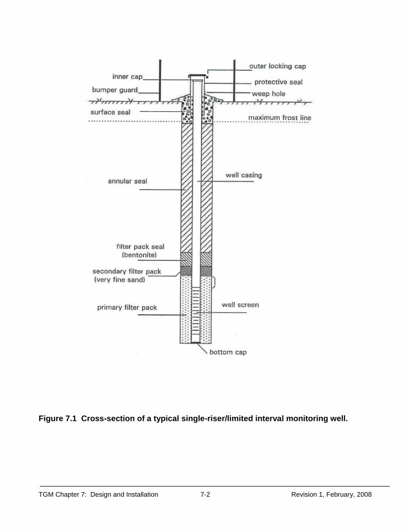
TGM Chapter 7: Design and Installation 7-2 Revision 1, February, 2008
Figure 7.1 Cross-section of a typical single-riser/limited interval monitoring well.
TGM Chapter 7: Design and Installation 7-3 Revision 1, February, 2008
WELL CLUSTERS When monitoring multiple intervals at one location, single-riser/limited interval wells are often installed in adjacent, separate boreholes. These well clusters can be used to determine vertical gradients when distinct differences in head exist. They may be used to monitor discrete zones or evaluate chemical stratification within a thick zone. If flow direction has been determined prior to installation, the shallow well should be placed hydraulically upgradient of the deeper well to avoid the potential influence on its samples caused by the presence of grout in the annular space of the deeper well. MULTI-LEVEL WELLS Multi-level wells allow sampling of more than one interval in a single borehole. These levels are isolated within the well either by packers or grout. Probes, lowered into the casing, can locate, isolate and open a valve into a port coupling to measure the fluid pressure outside the coupling or obtain a sample. Individual tubes run from sampling levels to the surface. The use of multiple-level monitoring wells in Ohio has been limited due to: 1) cost of installation, 2) difficulty in repairing clogs, and 3) difficulty in preventing and/or evaluating sealant and packer leakage. Detailed workplans (including construction and installation, methods to measure water levels and obtain samples, references to situations where these types of wells have been used successfully, and advantages and disadvantages) should be submitted prior to installing multi-level systems. Several systems are commercially available for obtaining multi-level monitoring of a single borehole. Most consist of casing or tubing with monitoring ports located at user-selected intervals. In one system, however, a lining containing intermittent sampling ports is placed in the borehole. The systems may be sampled with small diameter pumps and bailers, or using proprietary samplers that go with the monitoring system. See Nielsen and Schalla (2006) for more information on multi-level well systems. NESTED WELLS Nested wells involve the completion of a series of single-riser wells in a borehole. Each well is screened to monitor a specific zone, with filter packs and seals employed to isolate the zones. Nested wells are not recommended because they are difficult to install in a manner that ensures that all screens, filter packs, and seals are properly placed and functioning. It is more efficient to install single-riser wells for each interval to ensure that representative samples can be collected. Aller et al. (1991) indicated that individual completions generally are more economical at depths less than 80 feet. According to Nielsen and Schalla (2006), the cost of installing well clusters is comparable to the cost for nested wells. Well clusters can enable savings on sampling and future legal costs that may be necessary to prove the accuracy of nested wells.
TGM Chapter 7: Design and Installation 7-4 Revision 1, February, 2008
SINGLE-CASING, LONG-SCREEN WELLS Single-casing, long-screen wells are monitoring wells that, in general, are screened across the entire thickness of a water-bearing zone. If purging is performed immediately before sampling, only composite water samples are yielded, which are not adequate for most monitoring studies. If natural, flow-through conditions can be maintained, vertical water quality profiles can be obtained with passive sampling techniques. Vertical profiling may be a cost effective initial assessment to determine the depth of final wells. Long-screen wells are not appropriate for detection monitoring. Furthermore, these wells can allow cross-contamination between different zones and, therefore, should not be used in contaminated areas.
CASING The purpose of casing is to provide access to the subsurface for sampling of ground water and measurement of water levels. A variety of casing types have been developed. Items that must be considered during well design include casing type, coupling mechanism, diameter, and installation. CASING TYPES Three categories of casing are commonly used for ground water monitoring, including fluoropolymers, metallics, and thermoplastics (Aller et al., 1991). All have distinctive characteristics that determine their appropriateness. Fluoropolymers Fluoropolymers are synthetic plastics composed of organic material. They are resistant to chemical and biological attack, oxidation, weathering, and ultraviolet (UV) radiation. They have a broad useful temperature range, a high dielectric constant, a low coefficient of friction, display anti-stick properties, and have a greater coefficient of thermal expansion than most other plastics and materials (Aller et al., 1991). Standard properties of the various materials have been provided by Aller et al. (1991). The most common fluoropolymer used for monitoring wells is polytetrafluoroethylene (PTFE). It can withstand strong acids and organic solvents and, therefore, it is useful for environments characterized by the presence of these chemicals. It maintains a low tensile strength, which theoretically limits installation of Schedule 40 PTFE to an approximate depth of 250 ft1. It is also very flexible, which makes it difficult to install with the retention of straightness that is needed to ensure successful insertion of sampling or measurement devices. Dablow et al. (1988) found that the ductile nature of PTFE can result in the partial closing of screen slots
1 The maximum depth for PTFE casing depends on site hydrogeology. If the casing largely penetrates unsaturated soils, the depth may be limited to approximately 100 feet. However, if the casing is placed mostly in water-bearing zones, then depth may be as great as 375 feet.

TGM Chapter 7: Design and Installation 7-5 Revision 1, February, 2008
due to the compressive forces of the casing weight. This makes slot size selection very difficult. PTFE is costly, generally ten times more expensive than thermoplastics. Studies by Gillham and O’Hannesin (1990), Parker et al. (1990), and Parker and Raney (1993) (in Nielsen and Schalla, 2006), found that PTFE showed higher sorption rates than PVC of organic compounds. These studies concluded that PVC was a better material to use when organics are present. Metallics Metallic materials include low carbon, carbon, galvanized, and stainless steel. Metallics are very strong and rigid and can be used to virtually unlimited depths. Corrosion problems are the major disadvantage for low carbon, carbon, and galvanized casings, as electrochemical and chemical attack alters water sample quality. U.S.EPA (1992) has listed the following as indicators of corrosive conditions (modified from Driscoll, 1986):
Low pH (< 7.0). Dissolved oxygen exceeds 2 ppm. Hydrogen sulfide in quantities as low as 1 ppm. Total dissolved solids (TDS) greater than 1000 ppm. Carbon dioxide exceeds 50 ppm. Chloride (Cl-), bromide (Br-), and fluoride (F-) content together exceeds 500
ppm. According to Barcelona et al. (1983), flushing before sampling does not minimize the bias of low carbon steel due to the inability to predict the effects of disturbed surface coatings and corrosion products accumulated at the bottom of the well. Due to their high corrosion potential, all metallics except stainless steel are unacceptable for monitoring wells. Stainless steel is manufactured in two common types, 304 and 316. Type 304 is composed of iron with chromium and nickel. Type 316's composition is the same as Type 304's, but includes molybdenum, which provides further resistance to sulfuric acid solutions. Stainless steel is readily available in a wide variety of diameters. Stainless steel can perform quite well in most corrosive environments. In fact, oxygen contact develops an external layer that enhances corrosion resistance (Driscoll, 1986). However, several studies cite the formation of an iron oxide coating on the surface of stainless steel casing that forms in long-term exposure to ground water that can have unpredictable effects on the adsorption capacity of the casing material (Nielsen and Schalla, 2006). Under very corrosive conditions, stainless steel can corrode and release nickel and chromium into ground water samples (Barcelona et al., 1983). Combinations and/or extremes of the factors indicating corrosive conditions generally are an indication of highly corrosive environments. For example, Parker et al. (1990) found that both 304 and 316 showed rapid rusting (<24 hrs.) when exposed to water containing chloride above 1000 mg/l, and a study by Oakley and Korte (in Nielsen and Schalla, 2006) noted corrosion of stainless steel at even lower chloride levels (600-900 mg/L). Like PTFE, stainless steel is relatively expensive in comparison with thermoplastics. Nielsen and Schalla (2006) and Aller et al. (1991) provided additional information on the properties of stainless steel.
TGM Chapter 7: Design and Installation 7-6 Revision 1, February, 2008
Thermoplastics Thermoplastics are composed of large, synthetic organic molecules. The most common type used for monitoring wells is polyvinyl chloride (PVC), while a material used less often is acrylonitrile butadiene styrene (ABS). These materials are weaker, less rigid, and more temperature-sensitive than metallics. Thermoplastics are very popular due to their light weight, high strength to weight ratio, low maintenance, ease of joining, and low cost. Common, acceptable PVC types are Schedule 40 and Schedule 80. The greater wall thickness of Schedule 80 piping enhances durability and strength, provides greater resistance to heat attack from cement, and allows construction of deeper wells. Only rigid PVC should be used for monitoring wells. Flexible PVC is composed of a high percentage of plasticizers (30 - 50%), which tend to degrade and contaminate samples (Jones and Miller, 1988). All PVC casing should meet Standard 14 of NSF International. This standard sets control levels for the amount of chemical additives to minimize leaching of contaminants (NSF International, 1988). Additional specifications have been provided by Nielsen and Schalla (2006) and Aller et al. (1991). Drawbacks of PVC include brittleness caused by ultraviolet (UV) radiation, low tensile strength, relative buoyancy in water, and susceptibility to chemical attack. It is immune to corrosion and is resistant to most acids, oxidizing agents, salts, alkalies, oils, and fuels (NWWA/PPI, 1981). Additionally, Schmidt (1987) showed that no degradation of PVC occurred after six months immersion in common gasolines. However, studies have shown that high concentrations (parts-per-thousand or percentage concentrations) of tetrahydrafuran, methyl ethyl ketone, methyl isobutyl ketone, and cyclohexane degrade PVC (Nielsen and Schalla, 2006). Barcelona et al. (1983) reported that low molecular weight ketones, aldehydes, amines, and chlorinated alkenes and alkanes may cause degradation. Studies by Ranney and Parker (1995, 1997) and Parker and Ranney (1994b, 1995, 1996), showed that PVC is degraded when exposed to higher concentrations (0.2 and 0.4, or 20% and 40% of the solubility limit of the solvent in water) of aromatic hydrocarbons, aromatic and aliphatic chlorinated solvents, ketones, anilines, aldehydes and nitrogen-containing organic compounds. It is recommended that PVC not be used in situations where the material may be exposed to concentrations of known solvents or swelling agents of PVC greater than 25% of the solubility limit of the solvent or swelling agent (Nielsen and Schalla, 2006). TYPE SELECTION Many regulated parties choose PVC casing because of its lower cost; however, well integrity and sample representativeness are more important criteria. The high cost of analysis and the extreme precision of laboratory instruments necessitate the installation of wells that produce representative samples. Above all, the burden of proof is on the regulated party to demonstrate that casing is appropriate. The proper selection can be made by considering casing characteristics in conjunction with site conditions. Casing characteristics include strength, chemical resistance, and chemical interference potential. The strength must withstand the extensive tensile, compressive, and collapsing forces involved in maintaining an open borehole. Since the forces exerted are, in large part,
TGM Chapter 7: Design and Installation 7-7 Revision 1, February, 2008
related to well depth, strength often is important when planned depth exceeds the maximum range of the weakest acceptable material (100 to 375 ft. - PTFE). In these instances, either stainless steel or PVC should be chosen. Strength can be the overriding factor because the concern for chemical resistance and interference become insignificant if an open borehole cannot be maintained. Nielsen and Schalla (2006) provided specific strength data for commonly used materials. The casing also must withstand electrochemical corrosion and chemical attack from natural ground water and any contaminant(s). Chemical resistance is most important in highly corrosive environments, when contaminants are present at extremely high levels, and when wells are intended to be part of a long-term monitoring program. For extended monitoring in corrosive environments, PTFE and PVC are preferred over stainless steel because of the potential for the metallic material to degrade. If high concentrations of organics (parts per thousand) are present, either PTFE or stainless steel should be selected. PVC should not be used if a PVC solvent/softening agent is present or the aqueous concentration of a solvent/softening agent exceeds 25% of its solubility in water. It is suitable in most situations where low (parts per billion to low parts per million) levels of most organic constituents are present (Nielsen and Schalla, 2006). The casing also should not interfere with sample quality by adding (leaching) or removing contaminants. In most cases, the magnitude of this interference is a function of the ground water's contact time with the casing. The longer the contact, the greater the potential for leaching and sorption. Various studies have been conducted [Barcelona and Helfrich (1988), Curran and Tomson (1983), Gillham and O'Hannesin (1990), Jones and Miller (1988), Miller (1982), Parker and Jenkins (1986), Parker et al. (1990), Reynolds and Gillham (1985), Schmidt (1987), Sykes et al. (1986), Tomson et al. (1979), Hewitt (1992, 1994), Parker and Ranney (1994)] to compare the sorbing and leaching characteristics of the three favored materials. No conclusive results have been obtained to indicate that any one is best. Most of these studies involved contact lasting days, weeks, and even months and, therefore, the results cannot be correlated to field conditions where contact is often minimal because sampling is generally conducted soon after purging. In many cases, concern about sorption or leaching may be exaggerated. Barcelona et al. (1983) and Reynolds and Gillham (1985) both concluded that the potential sorption biases for casing may be discounted due to the short contact after purging. Also, Parker et al. (1990) indicated that sorption of various constituents never exceeded 10 percent in the first 8 hours of their tests. They concluded that, on the basis of overall sorption potential for organic and inorganic compounds, PVC is the best compromise. In summary, the appropriate casing should be determined on a case-by-case basis. PVC is acceptable when free product is not present and the solubility limits of organic contaminants are not approached (e.g., levels that exceed 0.25 times the solubility). Ohio EPA recognizes the difficulty inherent in establishing a "cut-off" level for when aqueous concentrations of organics cause failure of PVC. To be certain that casing will retain integrity, particularly when monitoring is planned for long periods of time (e.g., 30 years), Ohio EPA may recommend a more resistant casing when aqueous concentrations are relatively high but still below the criteria mentioned above.

TGM Chapter 7: Design and Installation 7-8 Revision 1, February, 2008
HYBRID WELLS Casing not in contact with the saturated zone generally is not subject to attack. Therefore, it may be possible to install less chemically resistant material above the highest seasonal water level and more inert material where ground water continually contacts the casing. Such a "hybrid well" commonly is installed to reduce costs. For example, when monitoring a zone with high concentrations of organics, stainless steel could be installed opposite the saturated materials, while PVC could be used opposite the unsaturated materials. Thus, resistant, more expensive casing would be present where contact with highly contaminated ground water may occur, while less resistant, inexpensive casing would be present where contact does not occur. Variations in ground water levels caused by seasonal or pumping effects should be taken into account when planning the casing material configuration (Nielsen and Schalla, 2006). Different varieties of steel never should be installed in the same well. Each type is characterized by its own electro-chemical properties. Installation of different types in contact can increase the potential for corrosion. COUPLING MECHANISMS Casing sections should be connected using threaded joints that provide for uniform inner and outer diameters along the entire length of the well. Such "flush" coupling is necessary to accommodate tools and sampling devices without obstruction and to help prevent bridging during the installation of the filter pack and annular seal. It should be noted that thread types vary between manufacturers and matching can be difficult. A union among non-matching joints should never be forced, otherwise structural integrity of the joint and the entire well could be compromised. To alleviate these problems, the American Society of Testing and Materials has developed Standard F 480-90 (1992) to create a uniformly manufactured flush-threaded joint. Most manufacturers now produce the F 480 joint, which is available in both PVC and stainless steel. Solvent cements should never be used because they are known to leach organics. Metal fasteners such as rivets or screws should not be used to supplement threaded joints. Use of such fasteners can reduce the effective inner well diameter, and may damage pumps or other tools lowered into the well (Nielsen and Schalla, 2006). It is recommended that either nitrile, ethylene propylene, or Viton O-rings be used between sections to prevent the seal and/or affected water from entering (Nielsen and Schalla, 2006). Nielsen and Schalla (2006) indicated that Teflon tape can be used in place of O-rings, although it does not ensure as good a seal. Although welding stainless steel can produce a flush joint that is of equal or greater strength than the casing itself, this method is not used as commonly as threaded joints due to the extra assembly time, welding difficulty, corrosion enhancement, ignition danger, and the potential to lose materials into the well (Nielsen and Schalla, 2006). Threaded steel casing provides inexpensive, convenient connections. It should be noted that threaded joints reduce the tensile strength of the casing; however, this does not cause a problem for most shallow wells. Also, threaded joints may limit or hinder the use of various sampling devices when thin-walled stainless steel (Schedules 5 and 10) is
TGM Chapter 7: Design and Installation 7-9 Revision 1, February, 2008
employed. Thin-walled casing is too thin for threads to be machined, so the factory welds a short, threaded section of Schedule 40 stainless steel pipe to the end of the thin-walled pipe. These joints are made to be flush on the outside, but not the inside. If hybrid wells are installed, it is essential that the joint threads be matched properly. This can be accomplished by purchasing casing screen that is manufactured to ASTM F480-90 (1992) standard coupling. DIAMETER Choice of casing diameter is site-specific. Small wells are considered to be less than 4 inches in diameter. Wells installed using conventional drilling methods are generally 2 or 4 inches in diameter. Wells installed by direct push technologies (see Chapter 15 – Use of Direct Push Technologies for Soil and Ground Water Sampling) have diameters of 2 inches to as small as 0.5 inch. Advantages of small diameter wells are as follows:
Water levels require less time to recover after purging. They produce a smaller volume of purged water that must be disposed. Construction costs are lower. They are more easily installed by driven, direct push, jetting, or hollow stem augers.
Some disadvantages of small diameter wells include:
Access may be limited for sampling devices. Filter packs and seals are more difficult to install. They offer a lower depth capability due to lesser wall thickness. Development can be more difficult. Less ground water is pumped during a hydraulic test or a remediation extraction. The amount of available water may be too small for chemical analyses. Slower recovery after water removal.
CASING INSTALLATION Casing should be cleaned thoroughly before installation. Strong detergents and even steam cleaning may be necessary to remove oils, cleansing solvents, lubricants, waxes, and other substances (Curran and Tomson, 1983; Barcelona et al., 1983). It is strongly recommended that only factory-cleaned materials be used for monitoring wells. Casing can be certified by the supplier and individually wrapped in sections to retain cleanliness. If it has not been factory-cleaned and sealed, it should be washed thoroughly with a non-phosphate, laboratory grade detergent (e.g., Liquinox) and rinsed with clean water or distilled/deionized water as suggested by Curran and Tomson (1983) and Barcelona et al. (1983). The materials should be stored in a clean, protected place to prevent contamination by drilling and site activities. When installing casing, it is important that it remain centered in the borehole to ensure proper placement and even distribution of the filter pack and annular seal. In addition, centering helps ensure straightness for sampling device access. If a hollow-stem auger is used, no additional measures are necessary because the auger acts as a centralizing device. If

TGM Chapter 7: Design and Installation 7-10 Revision 1, February, 2008
casing is installed in an open borehole, centralizers made of stainless steel or PVC can be used. They are adjustable and generally attached just above the screen and at 10 to 20 foot intervals along the riser. If centralizers are used, measures should be taken to prevent them from bridging the filter pack and seal material during their installation. If the well screen and riser are significantly lighter than the buoyant force of the fluid in the borehole, the casing assembly may require ballast to offset the tendency of the materials to float in the borehole. The riser may be ballasted by filling it with water of a known and acceptable source or with water previously removed from the borehole. Alternatively, hydraulic rams on the drill rig may be used to push the riser into the borehole (ASTM D5092-04).
INTAKES
Although every well is unique, most have a screen and filter pack comprising the well intake. Monitoring wells in cohesive bedrock may incorporate open borehole intakes. FILTER PACK Wells monitoring unconsolidated and some poorly consolidated materials typically need to have a screen (discussed later) surrounded by more hydraulically conductive material (filter pack). In essence, the filter pack increases the effective well diameter and prevents fine-grained material from entering. Types of Filter Packs Filter packs can be classified by two major categories, natural and artificial. Natural packs are created by allowing the formation to collapse around the screen. In general, natural packs are recommended for formations that are coarse-grained, permeable, and uniform in grain size. Grain size distribution of the formation should be determined through a sieve analysis of samples from the formation. According to Nielsen and Schalla (2006), natural packs may be suitable when the effective grain size (sieve size that retains 90%, or passes 10%) is greater than 0.010 inch and the uniformity coefficient (the ratio of the sieve size that retains 40% and the size that retains 90%) is greater than 3. Ideally, all fine-grained particles are removed when the well is developed, leaving the natural pack as a filter to the surrounding formation. Installation of artificial packs involves the direct placement of coarser-grained material around the screen. The presence of this filter allows the use of a larger slot size than if the screen were in direct contact with the formation. Artificial packs generally are necessary where: 1) the formation is poorly sorted; 2) the intake spans several formations and/or thin, highly stratified materials with diverse grain sizes; 3) the formation is a uniform fine sand, silt or clay; 4) the formation consists of thinly-bedded materials, poorly cemented sandstones, and highly weathered, fractured, and solution-channeled bedrock; 5) shales and coals that provide a constant source of turbidity are monitored; and 6) the borehole diameter is significantly greater than the diameter of the screen (Aller et al., 1991), (Nielsen and Schalla, 2006). Artificial packs generally are used opposite unconsolidated materials when the

TGM Chapter 7: Design and Installation 7-11 Revision 1, February, 2008
effective grain size is less than 0.010 inches and when the uniformity coefficient is less than 3.0 (Nielsen and Schalla, 2006). Pre-packed well screens (discussed below) may also be used to install an artificial filter pack. The filter pack for these screens is installed at the surface, ensuring an effective filter pack. An artificial pack may include two components. The primary pack extends from the bottom of the borehole to above the top of the screen. In some cases, it may be desirable to place a secondary pack directly on top of the primary pack. Its purpose is to prevent the infiltration of the annular seal into the primary pack, which can partially or totally seal the screen. Nature of Artificial Filter Pack Material The artificial pack material should be well-sorted, well-rounded, clean, chemically inert, of known origin, and free of all fine-grained clays, particles and organic material. Barcelona et al. (1983) recommended clean quartz sand or glass beads. Quartz is the best natural material due to its non-reactive properties and availability. Crushed limestone should never be used because of the irregular particle size and potential chemical effects. Materials should be washed, dried, and packaged at the factory, and typically are available in 100 lb. bags (approximately one cubic foot of material) (Nielsen and Schalla, 2006). The material should be based on the formation particle size. If chosen grains are too small, it is possible that loss of the pack to the formation can occur (Nielsen and Schalla, 2006), which could lead to the settling of the annular seal into the screened interval. On the other hand, if the grains are too large, the pack will not effectively filter fine-grained material, leading to excessively turbid samples. For these reasons, the universal application of a single well screen/filter pack combination to all formations should be avoided (ASTM D5092-04). The primary pack generally should range in grain size from a medium sand to a cobbled gravel. Most materials are available in ranges, such as 20- to 40-mesh (0.033 to 0.016 inches, Table 7.1). The grain size of the primary filter pack should be determined by multiplying the 70% retention size of the formation by a factor of 3 to 6 (U.S. EPA, 1975). A factor of 3 is used for fine, uniform formations; a factor of 6 is used for coarse, non-uniform formations. Where the material is less uniform and the uniformity coefficient ranges from 6 to 10, it may be necessary to use the 90% retention (10% passing) size multiplied by 6 (Nielsen and Schalla, 2006). This is to ensure that the bulk of the formation will be retained. The ratio of the particle size to the formation grain size should not exceed 6, otherwise, the pack will become clogged with fine-grained material from the formation (Lehr et al., 1988). If the ratio is less than 4, a smaller screen slot size will be necessary, full development of the well may not be possible, and well yield may be inhibited. When monitoring in very heterogeneous, layered stratigraphy, a type of pack should be chosen that suits the layer with the smallest grain size. It is preferred that the filter pack be of uniform grain size. Ideally, the uniformity coefficient should be as close to 1.0 as possible and should not exceed 2.5 (Nielsen and Schalla, 2006, ASTM D5092-04, 2005). Uniform material is much easier to install. If non-uniform material is used, differing fall velocities cause the materials to grade from coarse to fine upwards along the screen. This can result in the loss of the upper fine-grained portion to the well during development.

TGM Chapter 7: Design and Installation 7-12 Revision 1, February, 2008
The secondary filter pack material should consist of a 90% retention sieve size (10% passing) that is larger than the voids of the primary pack to prevent the secondary pack from entering the primary pack (Nielsen and Schalla, 2006). In general, the secondary 90% retention size should be one-third to one-fifth of the primary 90% retention size (Nielsen and Schalla, 2006). Dimension of Artificial Filter Pack The filter pack should be thick enough to completely surround the well screen. The well annulus should be large enough to preclude bridging of the filter-pack material. Centering of the well screen in the borehole will ensure adequate space for an effective filter pack. Driscoll (1986) states that the mechanical filtration function of the filter pack can be achieved with a filter pack of only 2 to 3 grains in thickness. Filter packs of less than a half inch thick have been successfully used in pre-packed well screens that are installed in direct push boreholes (Nielsen and Schalla, 2006). The primary pack should extend from the bottom of the screen to at least 3 feet above its top (Nielsen and Schalla, 2006). In deeper wells (i.e., >200 feet), the pack may not compress initially. Compression may occur after installation of the annular seal, which may allow the seal to be in close contact with the screen. Therefore, additional pack material may be needed to account for settling and, at the same time, provides adequate separation of the seal and the screen. However, extension of the pack should not be excessive because it enlarges the zone that contributes ground water to the well, which may cause excess dilution. The length of the secondary pack should be 1 foot or less. Artificial Filter Pack Installation Methods that have been used for artificial pack installation include tremie pipe, gravity emplacement, reverse circulation, and backwashing (Nielsen and Schalla, 2006). The material should be placed in a manner that prevents bridging and particle segregation. Bridging can cause large voids and may prevent material from reaching the intended depth. Segregation can cause a well to produce turbid samples. During installation, regular measurements with a weighted tape should be conducted to determine when the desired height has been reached, and also act as a tamping device to reduce bridging. The anticipated volume of filter pack should be calculated.2 Any discrepancy between the actual and calculated volumes should be explained.
2 Anticipated filter pack volume can be calculated by determining the difference in volume between the borehole and casing (using outside diameter of the well) from the bottom of the borehole to the appropriate height above the well screen.
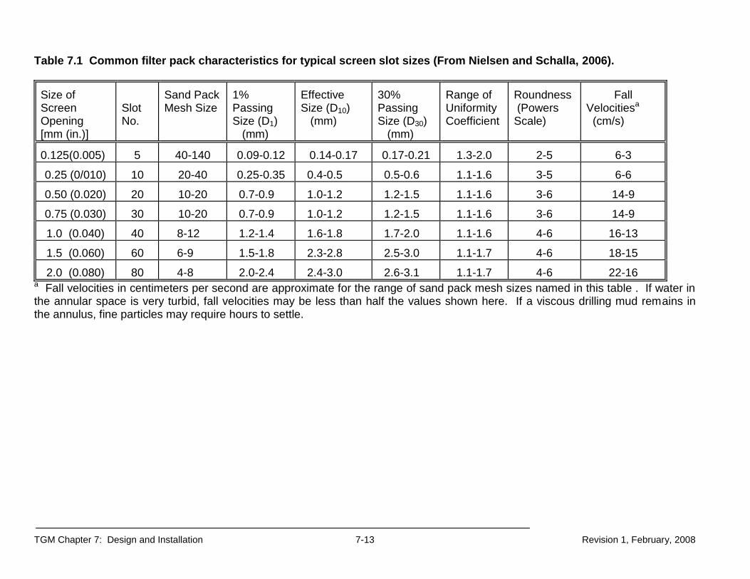
TGM Chapter 7: Design and Installation 7-13 Revision 1, February, 2008
Table 7.1 Common filter pack characteristics for typical screen slot sizes (From Nielsen and Schalla, 2006).
Size of Screen Opening [mm (in.)]
Slot No.
Sand Pack Mesh Size
1% Passing Size (D1) (mm)
Effective Size (D10) (mm)
30% Passing Size (D30) (mm)
Range of Uniformity Coefficient
Roundness (Powers Scale)
Fall Velocitiesa (cm/s)
0.125(0.005) 5 40-140 0.09-0.12 0.14-0.17 0.17-0.21 1.3-2.0 2-5 6-3
0.25 (0/010) 10 20-40 0.25-0.35 0.4-0.5 0.5-0.6 1.1-1.6 3-5 6-6
0.50 (0.020) 20 10-20 0.7-0.9 1.0-1.2 1.2-1.5 1.1-1.6 3-6 14-9
0.75 (0.030) 30 10-20 0.7-0.9 1.0-1.2 1.2-1.5 1.1-1.6 3-6 14-9
1.0 (0.040) 40 8-12 1.2-1.4 1.6-1.8 1.7-2.0 1.1-1.6 4-6 16-13
1.5 (0.060) 60 6-9 1.5-1.8 2.3-2.8 2.5-3.0 1.1-1.7 4-6 18-15
2.0 (0.080) 80 4-8 2.0-2.4 2.4-3.0 2.6-3.1 1.1-1.7 4-6 22-16 a Fall velocities in centimeters per second are approximate for the range of sand pack mesh sizes named in this table . If water in the annular space is very turbid, fall velocities may be less than half the values shown here. If a viscous drilling mud remains in the annulus, fine particles may require hours to settle.

TGM Chapter 7: Design and Installation 7-14 Revision 1, February, 2008
The preferred method for artificial pack installation is to use a tremie pipe to emplace material directly around the screen (Figure 7.2). The pipe is raised periodically to help minimize bridging. The pipe generally should be at least 1 inch ID, but larger diameters may be necessary where coarser-grained packs are being installed. When driven casing or hollow-stem augering is used to penetrate non-cohesive formations, the material should be tremied as the casing and auger is pulled back in one to two foot increments to reduce caving effects and ensure proper placement (Nielsen and Schalla, 2006). When installing wells through cohesive formations, the tremie pipe can be used after removal of the drilling device.
Figure 7.2. Installation of artificial filter pack material with a tremie pipe. (Source: Aller et al., 1991).

TGM Chapter 7: Design and Installation 7-15 Revision 1, February, 2008
Gravity emplacement is accomplished by allowing material to free-fall to the desired position around the screen. Placement by gravity should be restricted to shallow wells with an annular space greater than 2 inches, where the potential for bridging or segregation is minimized (Nielsen and Schalla, 2006). For low-yielding formations, it may be possible to bail the borehole dry to facilitate placement; however, segregation is generally not a problem if the pack has a uniformity coefficient of 2.5 or less. Gravity placement also can cause grading if the material is not uniform. In addition, formation materials are often incorporated during placement, which can contaminate the pack and reduce its effectiveness. For most cases, gravity placement is not recommended. Reverse circulation involves the insertion of a sand and water mixture through the annulus. Sand is deposited around the screen as the water returns to the surface through the casing. Due to the potential water quality alteration, this method generally is not recommended. Sand is deposited around the screen as the water returns to the surface through the casing. Due to the potential water quality alteration, this method generally is not recommended. Backwashing is accomplished by allowing material to free-fall through the annulus while clean water is pumped down the casing. The water returns up the annulus carrying fine-grained material with it. This creates a more uniform pack; however, the method is not commonly used for monitoring well installation and generally is not recommended due to the potential for alteration of ground water quality. Nonetheless, it is sometimes used for placing packs opposite non-cohesive heaving sands and silts. SCREEN The screen provides an access point to a specific portion of a ground water zone, as well as providing a barrier to keep unwanted formation particles out of ground water samples. Screen Types Recommended screen compositions are stainless steel, PTFE, and PVC. The same discussion and concerns for casing materials apply to screens. Only manufactured screens should be used, since these are available with slots sized precisely for specific grain sizes. Field-cut or punctured screen should never be used, due to the inability to produce the necessary slot size and the potential for the fresh surface to leach or sorb contaminants. A bottom cap or plug should be placed at the base of the screen to prevent sediments from entering and to ensure that all water enters the well through the screen openings. Slotted and continuous slot, wire-wound screen are the common types used for monitoring wells. In deep wells, slotted screen generally retains structural integrity better than wire-wound; however, continuous slot, wire-wound screens provide almost twice the open area of slotted casing. More open area per unit length enhances well recovery and development. A slot type should be chosen that provides the maximum amount of open area in relation to the effective porosity of the formation. Opinions vary regarding the optimum percentage of open area needed for effective hydraulic performance of well screens. Though it has been suggested that a range of open areas from 8 to 38% do not differ significantly in well performance, Driscoll (1986) recommended that the percentage of open area should be at least equal to the effective porosity of the formation and filter pack. In common situations

TGM Chapter 7: Design and Installation 7-16 Revision 1, February, 2008
with 8 to 30 percent effective porosities, continuous slot screens are preferred, although not required. A high percentage of open area is of greater importance when wells are installed in fine-grained formations where smaller slot sizes and fine-grained filter packs are required (Nielsen and Schalla, 2006). Pre-Packed Screen Wells
A pre-packed screen is an assembly consisting of an inner slotted screen surrounded by a wire mesh sleeve that acts as a support for filter media. The pre-packed screen assemblies can either be shipped with filter media already packed within the mesh sleeve or can be shipped without filter media and packed with filter sand in the field. Refer to ASTM D5092-04 for appropriate sizing of filter pack material. Pre-packed well screens help eliminate problems in the placement of filter pack around the screens of small diameter wells. In fine-grained formations pre-packed screens may be best for ensuring proper filter pack placement.
(ASTM D5092-04). The wells are sealed and grouted using the same procedure described for conventionally completed DPT wells. ASTM D6725-04 provides additional guidance on the use of pre-packed wells. Slot Size When selecting a screen slot size for an artificially filter-packed well, a sieve analysis should be conducted on the pack material. The selected size should retain at least 90% of the pack. In many situations it is preferable to retain 99% (Nielsen and Schalla, 2006 and ASTM D 5092-90, 1994). See Table 7.1 for a guide to the selection of slot sizes for various packs. For naturally-packed wells, the screen should retain at least 70% of the pack (Nielsen and Schalla, 2006, ASTM D5092-04). For additional information on pack and screen selection, see Aller et al. (1991), Nielsen and Schalla, (2006), and ASTM D 5092-90 (1994). It should be noted that if a PTFE screen is used in a deep well, a slightly larger slot size than predicted should be selected due to the material's lower compressive strength, which allows the openings to compress (Dablow et al., 1988). Length Screen length should be tailored to the desired zone and generally should not exceed 10 ft. A 2 to 5 ft. screen is desirable for more accurate sampling and discrete head measurements. Longer screens produce composite samples that may be diluted by uncontaminated water. As a result, concentrations of contaminants may be underestimated. In addition, if vertical flow is present, the well screen may provide a pathway for redistribution of contaminants, and possible cross-contamination of the formation (Nielsen and Schalla, 2006). Furthermore, the screen should not extend through more than one water-bearing zone to avoid cross-contamination. When a thick formation must be monitored, a cluster of individual, closely spaced wells, screened at various depths, can be installed to monitor the entire formation thickness. The length of screens that monitor the water table surface should account for seasonal fluctuation of the water table. For related information on screen length, refer to Chapter 5 – Monitoring Well Placement.

TGM Chapter 7: Design and Installation 7-17 Revision 1, February, 2008
OPEN BOREHOLE INTAKES When constructing monitoring wells in competent bedrock, an artificial intake is often unnecessary because an open hole can be maintained and sediment movement is limited. Installing a filter pack in these situations may be difficult due to loss of material into the surrounding formation. In some cases, however, intakes are a necessary component of bedrock wells. A screen and filter pack should be installed in highly weathered, poorly cemented, and fractured bedrock (Nielsen and Schalla, 2006). They are usually necessary when monitoring the unconsolidated/consolidated interface in Ohio. Open hole wells often are completed by casing and grouting the annulus prior to drilling into the monitoring zone. In cases where the zone has been drilled prior to sealing the annulus, a bridge (cement basket or formation packer shoe) must be set in the hole to retain the grout/slurry to the desired depth (Driscoll, 1986). If an open hole well is installed, the length of open hole generally should not exceed 10 feet to prevent sample dilution. To maintain a discrete monitoring zone in consolidated formations, the casing should be extended and grouted to the appropriate depth to maintain the 10 foot limit. Driven casing may be necessary to avoid loss of the annular seal into the surrounding formation.
ANNULAR SEALS The open, annular space between the borehole wall and the casing must be sealed properly to: 1) isolate a discrete zone, 2) prevent migration of surface water, 3) prevent vertical migration of ground water between strata, and 4) preserve confining conditions by preventing the upward migration of water along the casing. An effective seal requires that the annulus be filled completely with sealant and the physical integrity of the seal be maintained throughout the lifetime of the well (Aller et al., 1991). MATERIALS The sealant must be of very low permeability (generally 10-7 to 10-9 cm/sec), capable of bonding with casing, and chemically inert with the highest anticipated concentration of chemicals expected. Cuttings from the existing borehole, no matter what the type of materials, should never be used. They generally exhibit higher permeability and cannot form an adequate seal. The most common materials used are bentonite and neat cement grout. Each has specific, unique, and desirable properties. These materials are discussed briefly here. Additional information can be found in Michigan DEQ (2007), ASTM Method C-150 (2007), and Nielsen and Schalla (2006).

TGM Chapter 7: Design and Installation 7-18 Revision 1, February, 2008
Bentonite Bentonite is composed of clay particles that expand many times their original volume when hydrated. The most acceptable form is a sodium (Na) rich montmorillonite clay that exhibits a 10- to 12-fold expansion when hydrated. Other types, such as calcium (Ca) bentonite, are less desirable because they offer lower swelling ability and surface area to mass ratios. However, other types should be considered if Na bentonite is incompatible with the formation or analyses of concern. For example, the capability of bentonite may be adversely affected by chloride salts, acids, alcohols, ketones, and other polar compounds. Ca bentonite may be more appropriate for calcareous sediments. Bentonite is available in a variety of forms, including pelletized, coarse grade, granular and powder. Pellets are uniform in size and consist of compressed, powdered Na montmorillonite. They typically range from 1/4 to 1/2 inch in size. Pellets expand at a relatively slower rate when compared to other forms. Coarse grade, also referred to as crushed or chipped, consists of irregularly shaped, angular particles of montmorillonite that range from 1/4 to 3/4 inches in size. Granular particles range from 0.025 to 0.10 inches in size. Powdered bentonite is pulverized montmorillonite, factory-processed after mining. Powered and granular forms are generally mixed with water to form a slurry. Risk of losing a slurry to the underlying filter pack and surrounding formation should be considered. Bentonite slurry with less than 30 percent solids can lose its affinity for water, thus losing water to the formation (Listi, 1993). Bentonite used for drilling fluids/drilling fluid mud has a low solids content and therefore forms poor seals, so they are not suitable as annular seal materials (Edil et al., 1992). High-solids bentonite (>30% clay solids) has been developed specifically for monitoring well construction and provides an effective seal. High-solids bentonite slurries may also be formed by the addition of a swelling inhibitor to slow the swelling of the bentonite power, or addition of granular bentonite to bentonite slurry just prior to emplacement with a tremie pipe (Nielsen and Schalla, 2006). Neat Cement Grout Neat cement grout is comprised of portland cement and water, with no aggregates added. It is a hydraulic cement produced by pulverizing cement clinker consisting essentially of hydrated calcium silicates, and usually containing one or more forms of calcium sulfate as an interground addition. Several types of portland cements are manufactured to accommodate various conditions. Table 7.2 lists the types as classified by ASTM C150-07(2007). Type I is most commonly used for monitoring wells. Air-entraining portland cements have been specially processed to form minute air bubbles within the hardened structure. The air-entraining materials are added during the grinding of the clinker. The finished product is more resistant to freeze-thaw action. Air-entraining cements are designated with an "A" after the ASTM cement type. They have been used to construct water supply wells; however, they are less desirable than standard cements because of their greater permeability. Therefore, air-entraining varieties are not recommended for subsurface sealing of monitoring wells.

TGM Chapter 7: Design and Installation 7-19 Revision 1, February, 2008
Water added to the neat cement should be potable and contain less than 500 ppm total dissolved solids (Nielsen and Schalla, 2006). Low chloride and sulfate concentrations also are desirable (Campbell and Lehr, 1973). As the water to cement ratio increases, the compressive strength of the cement decreases and shrinkage increases. The American Petroleum Institute recommends a ratio of 5.2 gallons of water per 94 pound sack of cement. Additional water makes it easier to pump, but adversely affects the grout's sealing properties. Excess water can cause shrinkage and separation of the cement particles, which compromises seal integrity (Nielsen and Schalla, 2006). Table 7.2 ASTM cement designation (modified from Michigan DEQ, 2007).
CEMENT TYPE
DESCRIPTION
Type I
General purpose cement suitable where special properties are not required. Most common type of cement used for grouting.
Type II Moderate sulfate resistance. Lower heat of hydration than Type I.
Type III High early strength. Not commonly used. Ground to finer particle size, which increases surface area and reduces curing time period before drilling may resume from 48 hours to 12 hours.
Type IV Low heat of hydration cement designated for applications where the rate and amount of heat generated by the cement must be kept to a minimum. Develops strength at a lower rate than Type I. Not commonly used.
Type V Sulfate-resistant cement for use where ground water has a high sulfate content.
Type IA, IIA, and IIIA
Air entraining cements for the same use as Types I, II, and III. Not recommended for monitoring well construction.
The major disadvantages of neat cement are its heat of hydration, shrinkage upon curing, and its effect on water quality. During curing, heat is released, which is generally of little concern for monitoring wells. If large volumes of cement are used or the heat is not rapidly dissipated, the resulting high temperatures can compromise the integrity of PVC casing. However, the borehole for most monitoring wells is small, and heat significant enough to cause damage generally is not created. Shrinkage is undesirable because it causes cracks and voids. Bentonite is sometimes added to cement slurry to reduce shrinkage, the bentonite causing the mixture to expand as it hydrates and swells. Bentonite is also added to improve the cement’s workability, reduce the
TGM Chapter 7: Design and Installation 7-20 Revision 1, February, 2008
weight and density of the slurry, and reduce the set strength of the cement seal. Several authors, however, have shown bentonite to be chemically incompatible with cement so that the bentonite does not swell, and indeed reduces the capacity of the slurry to swell (Calhoun, 1988, Listi, 1993). Sodium ions in the bentonite are replaced by calcium ions in the cement through ion exchange, reducing the capacity of the bentonite to swell. Cement also releases OH- ions as it sets, which causes the bentonite to flocculate, reducing its swelling ability. Christman et. al (2002) found that cement-bentonite grout showed evidence of dryness and variable consistency. If used, cement-bentonite grout should be used with care (ASTM 5092-04, Cristman, et. al, 2002). Upon setting, neat cement grouts often lose water into the formation and affect water quality. Neat cement typically ranges in pH from 10 to 12; therefore, it is important to isolate the annular seal from the screen and filter pack. This may be accomplished by placing a very fine-grained secondary filter pack, 2 to 3 feet thick, above the primary filter pack (Nielsen and Schalla, 2006). SEAL DESIGN Annular seals should incorporate measures to prevent infiltration into the filter pack. Contact with the seal can cause sampled ground water to be artificially high in pH. Additionally, bentonite has a high cation exchange capacity, which may affect the chemistry of samples (Aller et al., 1991). In the saturated zone, a 2-foot pure bentonite seal can minimize the threat of infiltration. Above the bentonite seal, neat cement or bentonite grouts should be placed in the remainder of the annulus to within a few feet of the surface. SEAL INSTALLATION Bentonite Annular seals should be installed using techniques that prevent bridging, which may cause gaps, cracking or shrinking. Surface water and/or contaminants potentially can migrate through any voids created. Bentonite that comes in contact with ground water may affect the chemistry of the ground water due to its high pH and high cation exchange capacity. Cations in the molecular structure of the bentonite may exchange with cations existing in the ground water. Because of this, bentonite sealing material should be placed a minimum of 3 to 5 feet above the top of the well screen. Use of a secondary filter pack above the primary filter is also recommended (Nielsen and Schalla, 2006). The bentonite seal above the filter pack is commonly installed by placing granular bentonite, bentonite pellets, or bentonite chips around the casing by dropping them directly down the annulus. If feasible, this practice is acceptable for wells less than 30 feet deep if a tamping device is used. However, for wells deeper than 30 feet, coarse-grained bentonite should be placed by means of a tremie pipe. The bentonite should be allowed to hydrate or cure prior to sealing the remainder of the annular space. This will help prevent the grout from penetrating into the screened interval. Because bentonite chips or pellets requires a sufficient quantity and quality of water in order to achieve and retain hydration, bentonite chips or pellets generally should only be used in the saturated zone. If a two foot bentonite seal is desired in the unsaturated zone, granular bentonite should be used. It should be added and hydrated in lifts of 2 to 3 inches using water that is potable and free of analytes of concern (Nielsen and Schalla, 2006).

TGM Chapter 7: Design and Installation 7-21 Revision 1, February, 2008
For the remainder of the annulus, sealants should be in slurry form (e.g., cement grout, bentonite slurry) and should be placed with a tremie pipe (Figure 7.4). The grout should be mixed using a paddle-type mechanical mixer or by circulating the grout through a pump to disintegrate the lumps (ASTM 50-92-04). The grout should be placed with a tremie pipe. The bottom of the pipe should be equipped with a side discharge deflector to prevent the slurry from jetting a hole through the filter pack. The seal should be allowed to completely hydrate, set, or cure in conformance with the manufacturer's specifications prior to completing the surface seal and developing the well. Neat Cement Neat cement should not be poured into the annulus unless there is at least 3 inches between the casing and borehole, the annulus is dry, and the grout is being placed within 30 feet of the surface. If the neat cement grout is poured through standing water the mixture may be diluted or bridging may occur (Nielsen and Schalla, 2006). A neat cement grout should be mixed as with bentonite grout. A tremie pipe should be used for placement and inserted in the annulus to within a few inches of the bottom of the space using a side discharge port.
Figure 7.3 Tremie pipe emplacement of annular seal material (Source: Aller et l., 1991).

TGM Chapter 7: Design and Installation 7-22 Revision 1, February, 2008
SURFACE SEAL/PROTECTIVE CASING COMPLETIONS
A surface seal is used to prevent surface runoff from entering the well annulus. The surface seal and protective casing also serve to provide protection from accidental damage or vandalism. SURFACE SEAL A neat cement or concrete surface seal should be placed around a protective casing to a depth just below the frost line (3-5 ft.). If the same material was used in the annular seal, the surface seal can be a continuation; otherwise, the surface seal is installed directly over the annular seal after settling and curing. The surface seal should slope away from the well and extend beyond the edge of the borehole to divert surface water. Air-entraining cements may be desirable in cold climates to alleviate cracking caused by freezing and thawing. ABOVE-GROUND COMPLETIONS Whenever possible, monitoring wells should extend above the ground surface to prevent surface water from entering and to enhance visibility. From the frost line upward, a steel protective casing should encompass the well. The protective casing should be at least two inches larger in diameter than the inner casing, extend above it, and have a locking cap. The lock should be protected by plastic or rubber covers so the use of lubricants to free and maintain locking mechanisms can be avoided. A small drain or "weep hole" should be located just above the surface seal to prevent the accumulation of water between the casings (See Figure 7.1). This is especially useful in cold climates, where the freezing of trapped water can damage the inner casing. In areas susceptible to flooding, the protective casing should extend high enough to be above flood level (Nielsen and Schalla, 2006). A permanent reference point on the well inner casing must be surveyed to the nearest 0.01 ft. This permanent marker should be used for all water level measurements. Additionally, the well identification number or code should be marked permanently and clearly. Bumper or barrier guards should be placed beyond the edge of the surface seal or within 3 to 4 feet of the well (See Figure 7.1). These guards are necessary to reduce and prevent accidental damage from vehicles. Painting the guard posts yellow or orange and installing reflectors can increase visibility and help prevent mishaps. FLUSH-TO-GROUND COMPLETIONS Flush-to-ground completions are discouraged because the design increases the potential for surface water infiltration; however, they are occasionally unavoidable. This type of completion is generally used only when the location of a well would disrupt traffic areas such as streets, parking lots, and gas stations, or where easements require them (Nielsen and Schalla, 2006). If flush-to-ground completion is installed, very careful procedures should be followed. A secure subsurface vault generally is completed in the surface seal, allowing the well casing to be cut below grade. The vault should be traffic-rated, and constructed of steel, aluminum, or a high-strength plastic composite material (Nielsen and Schalla, 2006). An expandable locking cap on the casing and a water-proof gasket should be installed around the vault lid to

TGM Chapter 7: Design and Installation 7-23 Revision 1, February, 2008
prevent surface water infiltration. The gasket should be inspected at regular intervals and properly maintained to ensure a watertight seal (Nielsen and Schalla, 2006). The completion should be raised slightly above grade and sloped away to help divert surface water. It should be marked clearly and locked to restrict access. This is especially important at gas stations to prevent the misidentification of wells as underground tank filling points. In cold-weather areas where parking lots and roads may be cleared of snow with snowplows, the well vault should be set slightly below the surrounding concrete or asphalt to prevent shearing off of the vault lid by the blade of a snowplow. Flush-to-ground well completions should never be installed in low-lying areas that undergo flooding (Nielsen and Schalla, 2006).
DOCUMENTATION During monitoring well installation, pertinent information should be documented, including design and construction, the drilling procedure, and the materials encountered (see Chapter 3 for a listing of the particular geologic information needs). Accurate "as-built" diagrams should be prepared that, in general, include the following:
Date/time of start and completion of construction. Boring/well number. Drilling method and drilling fluid used. Borehole diameter and well casing diameter. Latitude and longitude. Well location (+ 0.5 ft.) with sketch of location. Borehole depth (+ 0.1 ft.). Well depth (+ 0.1 ft.). Casing length and materials. Screened interval(s). Screen materials, length, design, and slot size. Casing and screen joint type. Depth/elevation of top and bottom of screen. Filter pack material/size, volume calculations, and placement method. Depth/elevation to top and bottom of filter pack. Annular seal composition, volume, and placement method. Surface seal composition, placement method, and volume. Surface seal and well apron design/construction. Depth/elevation of water. Well development procedure and ground water turbidity. Type/design of protective casing. Well cap and lock. Ground surface elevation (+ 0.01 ft.). Surveyed reference point (+ 0.01 ft.) on well casing. Detailed drawing of well (include dimensions). Point where water encountered. Water level after completion of well development.
In addition, the following should be documented in work plans (when appropriate) and reports:

TGM Chapter 7: Design and Installation 7-24 Revision 1, February, 2008
Selection and rationale materials for selection of casing and screen. Selection and rationale for well diameter, screen length, and screen slot size. Filter pack selection and emplacement. Annular sealant selection and emplacement. Security measures. Locations and elevations of wells. Well development.
A complete, ongoing history of each well should be maintained. This can include sample collection dates, dates and procedures for development, water level elevation data, problems, repairs, personnel, and methods of decommissioning. This information should be kept as a permanent on-site file, available for agency review upon request. On July 18, 1990, Ohio House Bill 476 went into effect. This bill requires that all logs for monitoring wells drilled in Ohio be submitted to the Ohio Department of Natural Resources, Division of Water (ODNR). The ODNR can be contacted for further information.
MAINTENANCE AND REHABILITATION The condition of wells must be maintained to keep them operational and insure that representative samples can be obtained. The maintenance program should be site-specific and take into account all information that could affect well physical and chemical performance (ASTM Method D 5978-96(2005)). Maintenance consists of conducting inspections and periodic checks on performance. Proper documentation (see previous section) is needed to serve as a benchmark for evaluation, as well as to track well maintenance activities. Current conditions should be compared to as-built diagrams and previous measurements. Maintenance includes, but is not limited to, the following:
Ensuring visibility and accessibility. Inspecting locks for rusting. Inspecting surface pad and seals for cracking. Checking survey marks to insure visibility. Determining depth (see Chapter 10 for recommended procedures). Removing sediments (if needed). Evaluating performance by doing hydraulic conductivity tests. Evaluating turbidity and re-developing or replacing well if turbidity increases. Evaluating well construction using geophysical logs or down hole cameras.
TGM Chapter 7: Design and Installation 7-25 Revision 1, February, 2008
Routine inspections generally can be conducted during sampling. Additional evaluation can be conducted by comparing new ground water quality data and with previous data. If the maintenance check indicates a problem, rehabilitation should be conducted. Well rehabilitation activities include redevelopment to remove fine-grained materials or entrapped pollutants from the well. See Chapter 8: Monitoring Well Development for further information on well development.

TGM Chapter 7: Design and Installation 7-26 Revision 1, February, 2008
REFERENCES Aller, L., T. W. Bennett, G. Hackett, R. J. Petty, J. H. Lehr, H. Sedoris, D. M. Nielsen, and J.
E. Denne. 1991. Handbook of Suggested Practices for the Design and Installation of Ground-Water Monitoring Wells. Environmental Monitoring Systems Laboratory, Office of Research and Development, U.S. Environmental Protection Agency. Las Vegas, Nevada. EPA/600/4-89/034. (In cooperation with the National Water Well Association, Dublin, Ohio).
American Society For Testing and Materials (ASTM), Method C150 07. Standard
Specification for Portland Cement. Annual Book of American Society For Testing and Material Standards. Philadelphia, Pennsylvania Vol. 4.01, pp. 11-125.
ASTM, Method D5092-90 -04e1. Standard Practice for Design and Installation of Ground
Water Monitoring Wells in Aquifers. Annual Book of American Society for Testing and Material Standards. Philadelphia, Pennsylvania. Vol. 04.09, pp. 162-173.
ASTM Method D 5978-96 (2005). Standard Guide for Maintenance and Rehabilitation of
Ground-Water Monitoring Wells. American Society for Testing and Material Standards. West Conshohocken, Pennsylvania.
ASTM D 6725-04, Standard Practice for Direct Push Installation of Prepacked Screen
Monitoring Wells in Unconsolidated Aquifers. American Society for Testing and Material Standards. West Conshohocken, Pennsylvania.
ASTM, Method F480-90. Standard Specifications for Thermoplastic Well Casing Pipe and
Couplings Made in Standard Dimension Ratios (SDR) SCH40 and SCH80. Annual Book of American Society for Testing Material Standards. Philadelphia, Pennsylvania. Vol. 04.08, pp. 792-805.
Barcelona, M. J., J. P. Gibb and R. Miller. 1983. A Guide to the Selection of Materials for
Monitoring Well Construction and Ground Water Sampling. Illinois State Water Survey, SWS Contract Report 327. Champaign, Illinois.
Barcelona, M. J. and J. A. Helfrich. 1988. Laboratory and Field Studies of Well Casing
Material Effects. Proceedings of the Ground Water Geochemistry Conference. National Water Well Association. Dublin, Ohio. pp. 363-375.
Campbell, M. D. and J. H. Lehr. 1973. Water Well Technology. McGraw-Hill Book
Company. New York, New York. Calhoun, D. E., Sealing well casings: and idea whose time has come, 1988. Water Well
Journal, Volume 42, Number 2, pp. 25-29. Christman, M., C.H. Benson, T.B. Edil. 2002. Geophysical Study of Annular Well Seals.
Ground Water Monitoring and Remediation. Volume 22, Number 3, pp. 104-12. Curran, C. M. and M. B. Tomson. 1983. Leaching of Trace Organics into Water from Five
Common Plastics. Ground Water Monitoring Review. Vol. 3, No. 3, pp. 68-71.

TGM Chapter 7: Design and Installation 7-27 Revision 1, February, 2008
Dablow, J.S. III, D. Persico and G.R Walker. 1988. Design Considerations and Installation
Techniques for Monitoring Wells Cased with Teflon PTFE. In: A. J. Collins and A. I. Johnson (editors), Ground-Water Contamination Field Methods. ASTM STP 963. American Society for Testing Materials. Philadelphia, Pennsylvania. pp. 199-205.
Driscoll, F.G. (editor). 1986. Ground Water and Wells. Second Edition. Johnson Division.
St. Paul, Minnesota. Edil, T.B., M.M.K. Chang, L.T. Lan, T.V. Riewe. 1992. Sealing Characteristics of Selected
Grouts for Water Wells. Ground Water. Volume 30, Number 3, pp. 351-361. Einarson, Murray D., and John A. Cherry. A New Multilevel Ground Water Monitoring System
Using Multichannel Tubing, 2002. Ground Water Monitoring and Remediation, Volume 22, Number 4, pp. 52-65.
Gaber, M. S. and B. O. Fisher. 1988. Michigan Water Well Grouting Manual. Division of
Water Supply, Bureau of Environmental and Occupational Health, Michigan Department of Health. Lansing, Michigan.
Gillham, R. W. and S. F. O'Hannesin. 1990. Sorption of Aromatic Hydrocarbons by Materials
Used in the Construction of Groundwater Sampling Wells. Institute of Groundwater Research, University of Waterloo. Ontario, Canada.
Hewitt, A.D. 1994. Dynamic Study of Common Well Screen Materials. Ground Water
Monitoring and Remediation. Vol. 14, No. 1, pp. 87-94. Hewitt, A.D. 1992. Potential of Common Well Caseing Materials to Influence Aqueous Metal
Concentrations. Ground Water Monitoring Review. Vol. 12, No. 2, pp. 131-136. Jones, J. N. and G. D. Miller. 1988. Adsorption of Selected Organic Contaminants Onto
Possible Well Casing Materials. In: A. G. Collins and A. I. Johnson (editors), Ground-Water Contamination Field Methods. ASTM STP 963. American Society for Testing and Material Standards. Philadelphia, Pennsylvania. pp. 185-198.
Lehr, J. H., S. Hurlburt, B. Gallagher and J. Voytek. 1988. Design and Construction of Water
Wells. Van Nostrand Reinhold. New York, New York. Listi, R., Monitoring Well Grout: Why I think bentonite is better, 1993. Water Well Journal,
May, 5-6, 1993. Michigan Department of Environmental Quality, 2007. Ground Water & Wells Fundamentals
and Water Well Inspector’s Manual. Lansing, Michigan. Miller, G. D. 1982. Uptake and Release of Lead, Chromium, and Trace Level Volatile
Organics Exposed to Synthetic Well Casings. Proceedings of the Second National Symposium on Aquifer Restoration and Ground-Water Monitoring. National Water Well Association. Dublin, Ohio. pp. 236-245.

TGM Chapter 7: Design and Installation 7-28 Revision 1, February, 2008
NSF International. 2004. Plastic Piping Components and Related Materials, NSF Standard Number 14. Ann Arbor, Michigan.
Nielsen, D. M. and R. Schalla. 2006. Design and Installation of Ground Water Monitoring
Wells. In: David M. Nielsen (editor), Practical Handbook of Ground-Water Monitoring. Lewis Publishers, Inc. Chelsea, Michigan. pp. 639-806.
NWWA/Plastic Pipe Institute. 1981. Manual on the Selection and Installation of
Thermoplastic Water Well Casing. National Water Well Association. Worthington, Ohio. Parker, L. V. and T. F. Jenkins. 1986. Suitability of Polyvinyl Chloride Well Casings for
Monitoring Munitions in Ground Water. Ground Water Monitoring Review. Vol. 6, No. 3, pp. 92-98.
Parker, L. V., A. D. Hewitt, and T. F. Jenkins. 1990. Influence of Casing Materials on Trace-
Level Chemicals in Well Water. Ground Water Monitoring Review. Vol. 10, No. 2, pp. 146-156.
Parker, L.V. and T.A. Ranney, 1994. Effect of Concentration on Sorption of Dissolved
Organics by PVC, PTFE, and Stainless Steel Well Casings. Ground Water Monitoring and Remediation. Vol. 14, Vo. 3, pp. 139-149.
Reynolds, G. W. and R. W. Gillham. 1985. Absorption of Halogenated Organic Compounds
by Polymer Materials Commonly Used in Ground Water Monitoring. Proceedings of the Second Canadian/American Conference on Hydrogeology. National Water Well Association. Dublin, Ohio. pp. 198-204.
Rinaldo-Lee, M.B. 1983. Small vs. Large Diameter Monitoring Wells. Ground Water
Monitoring Review. Vol.3, No. 1, pp. 72-75. Schalla, R. and P. L. Oberlander. 1983. Variation in the Diameter of Monitoring Wells.
Water Well Journal.Vol. 37, No. 5, pp. 56-73.
Schmidt, K. D. 1982. The Case for Large Diameter Monitoring Wells. Water Well Journal.
Vol. 36, No. 12, pp. 28-29. Schmidt, G. W. 1987. The Use of PVC Casing and Screen in the Presence of Gasolines on
the Ground Water Table. Ground Water Monitoring Review. Vol. 7, No. 2, p. 94. Sykes, A. L., R. A. McAllister and J. B. Homolya. 1986. Sorption of Organics by Monitoring
Well Construction Materials. Ground Water Monitoring Review. Vol. 6, No. 4, pp. 44-48. Tomson, M. B., S. R. Hutchins, J. M. King and C. H. Ward. 1979. Trace Organic
Contamination of Ground Water: Methods for Study and Preliminary Results. Third World Congress on Water Resources. Vol. 8. Mexico City, Mexico. pp. 3701-3709.
U.S. EPA. 1975. Manual of Water Well Construction Practices. Office of Water Supply.
EPA/ 570/9-75-001.

TGM Chapter 7: Design and Installation 7-29 Revision 1, February, 2008
U.S. EPA. 1992. RCRA Ground-Water Monitoring: Draft Technical Guidance. Office of
Solid Waste. EPA/530/R/93-001, Dockette #F/93/GWMA/FFFF. Washington, D.C. Wisconsin Code. 1990. Ground Water Monitoring Requirements. Wisconsin Department of
Natural Resources. Chapter NR 141.01 to NR 141.31. Wisconsin Register No. 409.

State of Ohio Environmental Protection Agency
Division of Drinking and Ground Waters
Technical Guidance Manual for Ground Water Investigations Chapter 8
Monitoring Well Development, Maintenance, and Redevelopment
February 2009 Governor : Ted Strickand Director : Chris Korleski

TECHNICAL GUIDANCE MANUAL FOR
GROUND WATER INVESTIGATIONS
CHAPTER 8
MONITORING WELL DEVELOPMENT, MAINTENANCE, AND REDEVELOPMENT
February 2009 Revision 2
Ohio Environmental Protection Agency Division of Drinking and Ground Waters
P.O. Box 1049 50 W. Town Street, Suite 700 Columbus, Ohio 43216-1049
Phone: 614-644-2752 http://www.epa.state.oh.us/ddagw/

TGM Chapter 8: Development 8-i Revision 2, February 2009
PREFACE
This document is part of a series of chapters incorporated in Ohio EPA’s Technical Guidance Manual for Hydrogeologic Investigations and Ground Water Monitoring (TGM), which was originally published in 1995. DDAGW now maintains this technical guidance as a series of chapters rather than as an individual manual. The chapters can be obtained at http://www.epa.state.oh.us/ddagw/tgmweb.aspx. The TGM identifies technical considerations for performing hydrogeologic investigations and ground water monitoring at potential or known ground water pollution sources. The purpose is to enhance consistency within the Agency and inform the regulated community of the Agency’s technical recommendations and the basis for them. In Ohio, the authority over pollution sources is shared among various Ohio EPA divisions, including the Emergency and Remedial Response (DERR), Hazardous Waste Management (DHWM), Solid and Infectious Waste (DSIWM), and Surface Water (DSW), as well as other state and local agencies. DDAGW provides technical support to these divisions. Ohio EPA utilizes guidance to aid regulators and the regulated community in meeting laws, rules, regulations and policy. Guidance outlines recommended practices and explains their rationale. The Agency may not require an entity to follow methods recommended by this or any other guidance document. It may, however, require an entity to demonstrate that an alternate method produces data and information that meet the pertinent requirements. The procedures used to meet requirements usually should be tailored to the specific needs and circumstances of the individual site, project, and applicable regulatory program, and should not comprise a rigid step-by-step approach that is utilized in all situations.

TGM Chapter 8: Development 8-ii Revision 2, February 2009
MAJOR TECHNICAL CHANGES
Ohio EPA Technical Guidance Manual for Hydrogeologic Investigations and Ground Water Monitoring (TGM) was finalized in 1995 and Chapter 8 (Monitoring Well Development, Maintenance, and Redevelopment was revised in February 2004. This guidance document represents the second revision to Chapter 8. Listed below are the major changes from February 2004.
1. Revised the water quality indicator parameter values used to evaluate whether the well
has been properly developed.
2. Added a recommendation for a time interval between development and sampling of one week.

TGM Chapter 8: Development 8-iii Revision 2, February 2009
TABLE OF CONTENTS
PREFACE.................................................................................................................................. i MAJOR TECHNICAL CHANGES ............................................................................................. ii TABLE OF CONTENTS .......................................................................................................... iii FACTORS AFFECTING DEVELOPMENT .............................................................................. 1
HYDROGEOLOGIC ENVIRONMENT ................................................................................. 1 WELL DESIGN .................................................................................................................... 2 DRILLING METHODS ......................................................................................................... 3 PRESENCE OF NON-AQUEOUS PHASE LIQUIDS ........................................................... 3 INTENDED USE .................................................................................................................. 3 OTHER FACTORS .............................................................................................................. 3
DEVELOPMENT PROCEDURE .............................................................................................. 4 PREDEVELOPMENT .......................................................................................................... 4 DEVELOPMENT CRITERIA ................................................................................................ 4 METHODS ........................................................................................................................... 6
Pumping and Overpumping .............................................................................................. 6 Surging ............................................................................................................................. 7 Backwashing .................................................................................................................... 9 Bailing ............................................................................................................................... 9 Air-lift Pumping and Air Surging ....................................................................................... 9 Inertial Lift Pump............................................................................................................. 10
WELL DEVELOPMENT DOCUMENTATION ........................................................................ 11 TIME INTERVAL BETWEEN DEVELOPMENT AND SAMPLING ......................................... 11 WELL MAINTENANCE CHECKS AND REDEVELOPMENT ................................................ 13 REFERENCES ...................................................................................................................... 14
TGM Chapter 8: Development 8-1 Revision 2, February 2009
CHAPTER 8 MONITORING WELL DEVELOPMENT, MAINTENANCE, AND
REDEVELOPMENT The goal of ground water sampling is to obtain a sample that represents the current ground water conditions. Well development, well maintenance, and re-development (as needed) are critical to any ground water sampling program. The well development procedure and maintenance of the well should be documented. Due to the effects of installation, the ground water entering a monitoring well may not be representative of natural conditions with respect to yield, chemical characteristics, and amount of suspended particulate matter. To allow for the collection of representative samples or physical properties (e.g., hydraulic conductivity), wells must be developed properly. Development involves stressing the formation so that a graded filter pack is created around the screen and particulate matter and fluids (when used) remaining from well drilling and construction are removed. Development restores hydraulic conditions and enhances yield of the saturated zone, stabilizes chemical changes that may have occurred during drilling and construction, and produces a well that is capable of yielding a sample of acceptably low turbidity (Panko and Barth, 1988; Aller et al., 1991, Izraeli et al., 1992). Proper development creates a graded filter pack around the well screen. When pumping is first initiated, natural materials in a wide range of grain sizes are drawn into the well, producing very turbid water. As pumping continues, natural materials are drawn into the filter, producing an effective filter pack through a sorting process. This sorting process begins when the largest particles are retained by the filter pack, resulting in a layer of coarse particles against the screen. With continued pumping this process produces a progressively finer layer until an effective graded filter pack is produced (Izraeli, et al., 1992). As indicated above, a key aspect of development is that it can reduce sample turbidity by removing fine particulate matter (clay and silt) from the filter pack and the geologic formation near the well intake, enhancing inflow to the well. Additionally, it can increase the life of wells by reducing or eliminating the potential for filling with fine particles or organic matter. Such "silting up" reduces yield and can result in anaerobic activity (NCASI, 1981). It is essential that filtration not be viewed as a substitute for proper development.
FACTORS AFFECTING DEVELOPMENT Several factors may affect the performance and selection of a method or combination of methods for monitoring well development. These include, but may not be limited to, site hydrogeologic environment, well design, drilling method employed (Aller et al., 1991), and intended use of the well.
HYDROGEOLOGIC ENVIRONMENT Ground water moves more easily through permeable, consolidated formations and "clean", coarse-grained sand and gravel; therefore, development may be accomplished quickly and easily. In contrast, flow through relatively impermeable silty or clayey material is slow or

TGM Chapter 8: Development 8-2 Revision 2, February 2009
limited; consequently, the process can be difficult. Well development should be applied with great care to wells installed in predominantly fine-grained formations (e.g., silts and clays). Rigorous development techniques may actually increase the turbidity of the ground water. The ease of development is usually less predictable for unconsolidated formations than for rock. In general, more difficulty may be encountered when materials are unconsolidated. If a borehole is not stable, even distribution of the filter pack around the screen may not be achieved, hindering development (Aller et al., 1991). If materials are silt and clay, drilling may cause smearing along the borehole wall, which also causes problems. On the other hand, drilling causes minimal damage to homogeneous sand and gravel, and development is not affected (Hackett, 1987). Different types of formations may be developed more effectively by using certain techniques. For example, a highly stratified, coarse-grained deposit is handled best by methods that concentrate energy on small parts of the formation. If the deposit is rather uniform, techniques that apply the same force over the entire length of the well screen can produce satisfactory results. Techniques that withdraw water quickly can reduce the hydraulic conductivity of formations containing a significant amount of silt and clay (Driscoll, 1986). Development of fine-grained materials generally should be accomplished by gentle action (Gass, 1989).
WELL DESIGN Typical monitoring well design (e.g., small diameter, artificial filter pack, and limited screen open area) makes development difficult. Generally, wells should be designed to keep entrance velocities low enough to avoid degassing and/or alteration of water quality (Gass, 1986). The thickness of the pack has considerable effect on the procedure because it reduces the amount of energy imparted to the borehole wall. The pack should be as thin as possible if development is to be effective at removing fine particulates. Conversely, it should be thick enough to ensure adequate borehole support and good distribution of material around the screen. Generally, a minimum of two inches is sufficient. Selection of the proper screen slot size and configuration is also essential for successful development. Slots are chosen to permit removal of fine material from the formation (see Chapter 7). Large slots may filter too much material and cause settlement and damage. Alternatively, it may not be possible to develop or sample properly if the slots are too small. According to Driscoll (1986), development works best when screens have both maximum open area and a slot configuration that permits the forces to be directed efficiently into the formation. In general, screens that are continuous slot, wire-wound facilitate easier development because they have the greatest open area (Gass, 1986). Large diameter wells (i.e., four inches or larger) are much easier to develop due to equipment availability. However, the high cost of construction materials has resulted in the installation of smaller wells with machine-slotted screens (Gass, 1986). The equipment available for small diameter wells (e.g., direct push pre-packed wells) may be limited to small capacity bailers, inertial lift pumps, and small diameter bladder pumps.

TGM Chapter 8: Development 8-3 Revision 2, February 2009
DRILLING METHODS The drilling process influences not only choice of development procedures, but also the intensity with which the procedures should be applied (Aller et al., 1991). All drilling methods impair the ability of a formation to transmit water to a borehole or well. Problems that can occur include: 1) the use of air rotary drilling to penetrate consolidated rock can cause fine particles to build up on the borehole walls and may plug fractures and pore spaces, 2) driving casing or using augers can cause smearing of fine-grained particulates between the casing/screen and the natural formation, 3) mud rotary can cause mudcakes to build up on the borehole wall, and 4) all drilling methods potentially can compact sediments. Development should rectify these problems to enhance yield and allow collection of representative samples. Drilling fluid of any type can affect ground water quality; therefore, their use is discouraged. If a fluid is used, development should remove any that has infiltrated into the formation to allow in-situ ground water quality to return to pre-installation conditions.
PRESENCE OF NON-AQUEOUS PHASE LIQUIDS Prior to development, the well should be checked for the presence of non-aqueous phase liquids (NAPL). If present, consideration should be given to the degree the well should be developed or even if the well should be developed. Care will need to be taken so that development does not spread the NAPL across the entire screened interval (through the entire sand pack and along the adjacent formation.)
INTENDED USE The development technique may also depend on the intended use of a well. Wells intended for hydraulic testing (e.g., pump tests and slug tests) may need to be developed at higher rates to allow for the accurate determination of hydraulic conductivity and yield. Rates may need to be similar to the expected pumping rates anticipated during the aquifer tests. When the well will not be sampled for quality, other methods, such as jetting, may be acceptable (See Driscoll, 1986).
OTHER FACTORS Site accessibility and type and availability of equipment should be considered during the selection of an appropriate method or combination of methods. The need for proper disposal of contaminated discharge water also can drive selection. Time and cost may dictate selection; however, methods that minimize time and cost often prove to be inadequate. Cost/benefit analysis generally favors proper and complete development. If it is inadequate, time and cost for drilling, well installation, ground water sampling, and sample analysis may be wasted on data that is not representative Development should be applied cautiously to wells that are known or suspected to contain contaminants, particularly those that pose a hazard through inhalation or direct contact. Appropriate safety precautions should be taken to protect field personnel. Also, it should be
TGM Chapter 8: Development 8-4 Revision 2, February 2009
noted that contaminated water and sediments removed during development may need to be drummed and disposed of properly.
DEVELOPMENT PROCEDURE The general approach to development involves dislodging and removing fine-grained material and drilling fluids out of the ground water zone and into the well, and then from the well itself. This section describes development procedures, including predevelopment (measures taken during installation and construction), time and duration of development, and development methods.
PREDEVELOPMENT Whenever possible, steps should be taken during well installation and construction to remove drilling cuttings and fluids prior to placement of the screen, filter pack, and annual seal. This may include removing water from the borehole prior to installation of the well screen and surging and removal of water after the sand pack has been installed, prior to installing the annular seal. Typically, the water in the borehole is highly turbid and viscous from the drill cuttings. Removing this fluid prior to installing the screen and sand pack may make subsequent development efforts easier. An additional advantage to this technique is that the potential for "bridging" the sand pack during installation may be reduced because the viscosity of the water due to sediments in the boring is greatly reduced. After the screen and sand pack are in place the well may be surged gently prior to installing the bentonite seal and grout (note that the augers/casing should be at the top of the sand pack during this process to prevent overlying material from falling into the sand pack). Surging at this time is advantageous in that it will be more effective in removing fines from the well and formation and grading and stabilizing the sand pack when the weight of the overlying grout is not present. Additional sand may need to be added to compensate for settling of the sand pack and ensure that sufficient separation exists between the annular seal and well intake. If surging is performed only after the well is completely installed (i.e., the grout is in place), there is a greater chance that the sand pack could settle and create a void between the sand pack and annular seal. If the annular seal sinks into the void space, the well could become contaminated with grout and may need to be replaced. Mechanically surging the well using the drill rig is likely to be more effective and is much easier than trying to do it manually after the well is installed. Care should be taken not to place to large a force on the well that may cause it to collapse.
DEVELOPMENT CRITERIA Development should not be implemented until the seal has cured and settled. Ideally, a time of 48 hours is required for neat cement and bentonite grout mixtures (Gaber and Fisher, 1988). However, the time required varies with site conditions and grout type.

TGM Chapter 8: Development 8-5 Revision 2, February 2009
The duration of development varies with the type of formation, screen length, height of the water column, thickness of filter pack, and method used. The most frequent mistake is to “give up” before the well has been adequately developed. Adequate development may take less than two hours to more than three days. Development should proceed until the following criteria are met:
1. Water can enter as readily as hydraulic conditions allow.
2. A representative sample can be collected. In general, representative conditions can be assumed when the water is visually clear of sediments (e.g., turbidity 10 NTU) and pH, and specific conductance have stabilized over at least three successive well volumes. Other criteria such as temperature, oxidation-reduction potential or dissolved oxygen may also be useful to determine whether a well can produce a representative sample. Stability criteria of water quality parameters listed in Table 8.1 can be used to determine when development objectives have been met. The duration, along with pH, temperature, specific conductivity measurements, and turbidity should be recorded on the well development record (See section on Development Documentation).
In some instances, collection of a sample with a turbidity of 10 NTU is difficult or unattainable. If a well does not provide a sediment-free sample, development can stop when all of the following conditions are met:
• Several procedures have been tried, • Proper well construction has been verified, • Turbidity has stabilized within 10% over three successive well volumes, and • Conductivity, and pH have stabilized over at least three successive well volumes.
(It should be noted that pH, temperature, and conductivity may not stabilize if water quality has been degraded).
3. The sediment thickness remaining in the well is less than 1 percent of the screen
length or less than 0.1 feet for screens equal to or less than 10 feet.
4. A minimum of three times the standing water volume in the well (to include the well screen, casing, plus saturated annulus, assuming 30 percent annular porosity) should be removed. In addition to the “three times standing water volume” criteria, further volumetric removal should be considered if fluids were utilized during well drilling and installation.

TGM Chapter 8: Development 8-6 Revision 2, February 2009
Table 8.1. Water-Quality Indicator Parameters (ASTM Standard D6771-02).
Parameter Stabilization Criteria pH Difference of ±0.2 specific electric conductance Difference of ± 3% temperature Difference of ± 0.5 ºC turbidity ±10% (when turbidity is greater than 10 NTUs) oxidation -reduction potential (ORP) ± 20 millivolts dissolved oxygen (DO) 10% or ±0.2 mg/L, whichever is greater
METHODS In general, methods to develop monitoring wells include pumping, overpumping, surging, bailing, and backwashing. The most effective approach(s) generally is a combination of one or more methods that allow for water movement in both directions through the screen. A technique that allows for reversing the flow helps to minimize bridging in the formation and filter pack. Other methods exist, such as airlifting, air surging, jetting with water or air, or adding chemicals. Although various chemicals, including acids, surfactants, chelating agents, wetting agents, disinfectants, and dry ice have been employed for water supply wells, their use for monitoring wells is generally not appropriate. The addition of air, water, or chemicals may affect sample analysis in unpredictable ways. Air forced into a formation can reduce its permeability (Kraemer et al., 1991) and can cause volatilization of organics, if present. Water should be added only on rare occasions (i.e., when an insufficient amount exists to provide enough energy to develop the wells adequately). If water is added, it should be chemically analyzed for potential impact on in-situ ground water quality. The following provides a general description of methods commonly used. The advantages and disadvantages of each are summarized and procedures are provided. Pumping and Overpumping A widely accepted technique is to pump a well using an intake that is raised and lowered (without excessive surging) throughout the length of the screened interval (Puls and Powell, 1992). Methods that rely totally on pumping may not sufficiently stabilize the formation or the filter pack material. Although visibly clear water may eventually be discharged, any subsequent activity that agitates the water column can cause considerable turbidity (ASTM Standard D5521-05). Utilizing pumps in which the pumping action creates gentle surging or pumps that can be fitted with a surge block may enhance development. Backwashing may also be combined with pumping to create a surging action. The recommended approach is to begin pumping at the top of the screen with low pumping rates and incrementally work down the well screen. The process should then be repeated in reverse, from the bottom of the well to the top. When there is no improvement in turbidity, the well should be allowed to equilibrate and then the process should be repeated at higher pumping rates. Alternate pumping and equilibration cycles should continue until the water is free of sediments and no additional sediment accumulates in the bottom of the well.

TGM Chapter 8: Development 8-7 Revision 2, February 2009
According to Keely and Boateng (1987), however, some settlement and further loosening of fines can occur after the first attempt. Accordingly, a final series of cycles may need to be conducted 24 hours later. Monitoring well development should begin at low rates (e.g., 100 ml/min) and end at rates at least ten times the sampling rate; however, in most cases, higher rates will be needed. In particular, higher rates may be needed when the well is being used in hydraulic tests to determine hydraulic characteristics of the formation. Overpumping at a rate that substantially exceeds water removal during purging and sampling increases influx of fine particles, thereby opening screen slots, pore spaces, and fractures. High rates may not be advisable when wells are in a pristine area and adjacent to a contaminant plume because of the potential to draw in contaminants. Other disadvantages of pumping and overpumping include bridging of particles against the screen and the need for proper disposal of contaminated water. Development by pumping is most effective in coarse-grained, unconsolidated deposits and rock formations. However, it generally has limited application in highly conductive formations because it is difficult to pump monitoring wells at sufficient rates to create the high entrance velocities necessary for removal of fine particulates (Barcelona et al., 1985). The pumps utilized should be capable of pumping at low to high rates and be controlled by valving. Small diameter pumps that offer a wide range have recently been developed. Monitoring wells can be developed by using either a centrifugal or submersible pump. A centrifugal pump may be effective for low-yielding wells; however, it can be utilized only if the depth to water is less than approximately 25 feet. The use of a submersible pump is not limited by water level, but is affected by well diameter, construction material of the impeller, and type and concentration of contaminants. According to Kraemer et al. (1991), the presence of fine-grained materials can clog or damage pumps with plastic impellers. The bladder of squeeze-type pumps also may be damaged by fines. It is recommended that a bailer be initially used to remove accumulated sediments. Prior to well development, the pumps should be decontaminated in a manner consistent with the procedures described in Chapter 6 for drilling and subsurface sampling equipment. Surging Surging involves pulling and pushing water into and out of a well intake by using a plunger or block. This process destroys bridging and can be effective for small diameter monitoring wells. A surge block is a device with a flexible gasket that is close in size to the well diameter (Figure 8.1). It is attached to a rod that is raised and lowered. Water is forced out of the intake on the downstroke, breaking up the bridged sediments and enabling water and sediments to flow back into the well on the upstroke. The surge block should fit with a minimum clearance of one-fourth inch (Barcelona et al., 1985). It should be of sufficient weight to overcome the inertia and drag of the cable reel and friction of the discs against the casing on the downstroke. Also, it should be of sufficient density to overcome the effects of buoyancy (Schalla and Landick, 1986). Prior to surging, wells should be bailed or pumped to make sure that water will enter the well. If water does not enter the well, then surging should not be conducted. The negative pressure on the upstroke can cause the well to collapse.

TGM Chapter 8: Development 8-8 Revision 2, February 2009
For screen lengths of five feet or less, surging above the screen is effective for the entire screen length (Gass, 1986). For lengths greater than five feet, surging should be initiated above the screen and worked gradually downward at 2-3 feet intervals as water begins to easily move in and out of the well screen. To minimize damage, surging should start slowly and increase in force during the process. High differential pressures may cause collapse of the well screen or casing or may damage the filter pack (e.g., channels or voids may form near the screen if the pack sloughs away) (Keely and Boateng, 1987). A significant amount of fines can accumulate in the well during surging. These fines can be forced back into the formation and also make it impossible to remove the surge block. Therefore, it is necessary to withdraw the block at intervals and remove the sediment with a sand pump or bailer. According to a study by Paul et al. (1988), surging of wells screened in fine-grained sediments should be avoided because it increases turbidity, does not improve hydraulic response significantly, and is unnecessarily costly. However, gentle surging action to agitate the sand pack may assist in improving the turbidity of low-yielding saturated zones.
Figure 8.1 Development with a surge block (Source: “Monitoring Well Development” by T.E. Gass. Water Well Journal, Vol. 40, No. 1, p. 53 (Figure 1). 1986. Reprinted from Water Well Journal with permission from National Ground Water Association. Copyright 1986).

TGM Chapter 8: Development 8-9 Revision 2, February 2009
Backwashing Backwashing or rawhiding (Gass, 1986) involves allowing water that is pumped to the top of a well to flow back through the pump and out through the well intake. Backwashing breaks up the bridged particles, allowing them to be pumped and removed; however, it may not be forceful enough to obtain favorable results. The method may only develop materials opposite the upper part of the intake or preferentially develop the most permeable zones in stratified deposits. Also, it may allow potentially contaminated water to enter uncontaminated zones. Thus, the technique may not be appropriate for areas of known or suspected contamination. Bailing In some instances, a bailer with a check valve at the bottom may be an effective method of development (Lapham, et. al., 1997). The bailer is rapidly lowered down the well until it hits the water column. The impact of the bailer on the water surface will initially force water into the formation. The withdrawal of the bailer causes water to flow back into the well. A stainless steel bailer is recommended to have sufficient weight to create the surging action. A bailer can also be fitted with a flange to serve as a surging tool. To properly develop the well, rapid motions along the entire length of the intake should be done to create an inward and outward thrust of water that breaks up bridges that may have formed adjacent to the well intake. To enhance the removal of particulates accumulated at the bottom of the well, rapid short strokes near the bottom can be used to agitate and suspend sediments, thus allowing them to be removed. Development by bailing should be limited to gentle action in low-yielding wells (Gass, 1989). If a well is de-watered, it should be allowed to recover and bailing should be resumed. Development by bailing is very labor-intensive. Depending on the volume of water that must be removed, it may be useful to rig a tripod and pulley to aid in the lifting of the bailer from the well (Kraemer et al., 1991). As with surging, care should be taken not to cause collapse of the well casing or screen. Air-lift Pumping and Air Surging Other techniques commonly utilized are air lift pumping and air surging. These methods may induce and trap air in the formation outside the well intake and alter ground water quality. Furthermore, if ground water is highly contaminated, the methods can expose field personnel to hazardous materials. Use is not recommended unless the technique does not introduce air into the well screen and it can be demonstrated that the quality of water to be sampled will not be affected. Air from the compressor should be filtered to insure that oil is not introduced into the well (Barcelona et al., 1985). Generally, air techniques may be effective at removing debris, but cause very little positive effect beyond the well screen (Gass, 1986). One method that does not introduce air is two pipe air-lift pumping (Figure 8.2). Air is injected through the inner pipe at high pressure to bubble out into the surrounding outer pipe. The bubbles reduce the unit weight of the water, causing the column of water and sediments to be lifted upward, allowing ground water from the formation to flow into the well (Gass, 1986).
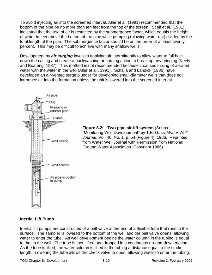
TGM Chapter 8: Development 8-10 Revision 2, February 2009
To avoid injecting air into the screened interval, Aller et al. (1991) recommended that the bottom of the pipe be no more than ten feet from the top of the screen. Scalf et al. (1981) indicated that the use of air is restricted by the submergence factor, which equals the height of water in feet above the bottom of the pipe while pumping (blowing water out) divided by the total length of the pipe. The submergence factor should be on the order of at least twenty percent. This may be difficult to achieve with many shallow wells. Development by air surging involves applying air intermittently to allow water to fall back down the casing and create a backwashing or surging action to break up any bridging (Keely and Boateng, 1987). This method is not recommended because it causes mixing of aerated water with the water in the well (Aller et al., 1991). Schalla and Landick (1986) have developed an air-vented surge plunger for developing small-diameter wells that does not introduce air into the formation unless the unit is lowered into the screened interval.
Figure 8.2: Two pipe air-lift system (Source: “Monitoring Well Development” by T.E. Gass. Water Well Journal, Vol. 40, No. 1, p. 54 (Figure 4). 1986. Reprinted from Water Well Journal with Permission from National Ground Water Association. Copyright 1986).
Inertial Lift Pump Inertial lift pumps are constructed of a ball valve at the end of a flexible tube that runs to the surface. The sampler is lowered to the bottom of the well and the ball valve opens, allowing water to enter the tube. As well development begins the water column in the tubing is equal to that in the well. The tube is then lifted and dropped in a continuous up-and-down motion. As the tube is lifted, the water column is lifted in the tubing a distance equal to the stroke length. Lowering the tube allows the check valve to open, allowing water to enter the tubing.

TGM Chapter 8: Development 8-11 Revision 2, February 2009
The ball valve seats on the upstroke, capturing the water that has entered the tubing. This cycle continues with each up and down movement until water moves up and out of the tubing. Inertial lift pumps are inexpensive, fairly portable, and easy to operate. They are particularly useful for development of small diameter wells (e.g., direct push pre-packed wells), since the tubing is available in sizes small enough to fit in small diameter wells. A potential drawback to inertial lift pumps is that in fine-grained formations over-surging can cause the well screen to become clogged with fines; therefore, it may be necessary to perform additional purging with a non-surging pump device to reduce turbidity (ASTM Standard D6724-04). Inertial lift pumps may be ineffective in removing large volumes of water and are not effective development tools for wells larger than 2 inches ID (ASTM Standard D6725-04). Use of an inertial lift pump that is close in size to the inner diameter of the well can create a surging action in the well, while the pump simultaneously purges the well, removing the fines that are loosened by the surging action. Attachable surge blocks are available for some inertial lift pumps; however, this can increase the risk of clogging.
WELL DEVELOPMENT DOCUMENTATION Well development documentation is important to show that representative samples can be obtained. Development method(s), time spent on development, volume of water removed, depth of the well, depth to top of the screen, diameter of the well, visual appearance (clarity), turbidity, pH, and specific electrical conductance of discharge water at various intervals should be recorded on a form or log (Lapham, et. al., 1997). Figure 8.3 provides an example of a well development record. Information on recovery rates and estimated yield should also be documented. This information may be helpful in planning for sampling events and in sampling techniques.
TIME INTERVAL BETWEEN DEVELOPMENT AND SAMPLING Prior to sampling a well, sufficient time should be allowed for equilibration with the formation after development. The intent is to provide time for the newly installed well and backfill materials to equilibrate to their new environment and for that environment to stabilize after disturbance. Though a significant volume of water may be pulled through the well during development, the well and granular backfill surfaces over which this water passes are not likely to be at chemical equilibrium with the ground water zone. The time for a well to stabilize depends on the characteristics of the ground water zone and the method of development; however, there is no rigorous scientific analysis to substantiate a time frame. A recommended “rule –of –thumb” is one week. Several weeks may be needed for lower permeability formations (< 1X 10⁻⁶ cm/sec) (Izraeli, et al, 1992; Byrnes et al., 1994; USACE, 1998). See section on “Development Criteria” for additional information on when a well can be considered properly developed.

TGM Chapter 8: Development 8-12 Revision 2, February 2009
Figure 8.3 EXAMPLE RECORD OF WELL DEVELOPMENT
Site Name: Initial Well Depth: Final Well Depth: Well ID: Well Diameter: Screen Length: Developers: Static Water Level: Total Purged Volume: Start Date: End Date: Weather Conditions: General Comments (e.g., presence of NAPLS): General Development Method(s):
Date Time Method Pumping
Rate (gal/min)
Volume Purged
(gal)
Temp. (ºC)
Spec. Cond.
(µS/cm) pH
Turbidity (NTU)
Other
Comments (e.g., clarity of water and success of development)
Field Parameter and Stability Guidance: pH (±0.2 standard units); Temperature (±0.5 ºC); specific conductance (±3%, µS/cm); turbidity (±10% when turbidity is greater than 10 NTU); dissolved oxygen ( 10% or ±0.2 mg/L, whichever is greater); oxidation-reduction potential ( ±20 ml/g) NTU- nephelometric unit, µS/cm- microsiemens per centimeter
TGM Chapter 8: Development 8-13 Revision 2, February 2009
WELL MAINTENANCE CHECKS AND REDEVELOPMENT
During the course of their active lives, monitoring wells should be checked to confirm that the well is still intact and fine particles have not accumulated. Unlike water supply wells, monitoring wells remain predominantly unpumped. There is no continuous removal of fines over an extended period. According to Kraemer et al. (1991), no matter how complete development appears to be, there is a high probability (especially for wells completed in fine-grained formations) that introduction of pumps or bailers will create a surge rendering the water somewhat turbid. In addition to sediments accumulating in the well, the casing and screen can become corroded or plugged by chemical or bio-chemical precipitates, and thus cause a loss of hydraulic connection. Metal well casings are subject to degradation over time from exposure to corrosive ground waters (pH of less than 6.0). Polyvinyl chloride (PVC) casing can dissolve in the presence of PVC solvent or if a pure organic product reaches the well in high concentrations from chemical spills or leaking storage tanks. A deteriorating well structure or a well that is “silting up” can cause a bias to the data that might be difficult to detect or might even be interpreted as trends in ground water quality. To provide a representative sample, these wells should be restored. Restoration typically involves redevelopment. It is recommended that performance be evaluated during the life of a well. This may include, but not be limited to, noting a significant drop in yield during purging, noting increased turbidity, measuring total well depth to determine if sediments have been deposited, and using a camera to determine if incrustation of the screen or damage to the well casing has occurred. Comparison of water-level fluctuations over time in the well can indicate a possible change in hydraulic connection of the well to the aquifer. For example, a long-term decline in the water level in a well could indicate gradual plugging of the well screen. Slug tests or injection, pressure, or partial-vacuum tests can also be conducted as part of the continual evaluation of the well (Stallman, 1983; Lohman, 1972; Driscoll, 1986; Bedinger and Reed, 1988). These tests help evaluate whether there is still good hydraulic connection between the well screen and the ground water zone. Well maintenance records should be kept including, but not limited to, periodic checks on depths; trends in water levels, yield changes and turbidity; the external physical condition of the well, its protective casing, the surface seal; and other criteria utilized to monitor the integrity of the well. At minimum, wells should be redeveloped when 20% of the well screen is occluded by sediments (U.S. EPA, 1988), or records indicate a change in yield and turbidity.

TGM Chapter 8: Development 8-14 Revision 2, February 2009
REFERENCES Aller, L., T. W. Bennett, G. Hackett, R. J. Petty, J. H. Lehr, H. Sedoris, D.M. Nielsen, and J.
E. Denne. 1991. Handbook of Suggested Practices for the Design and Installation of Ground Water Monitoring Wells. Environmental Monitoring Systems Laboratory, Office of Research and Development, U.S. Environmental Protection Agency. Las Vegas, Nevada. EPA/600/4-89/034. (In cooperation with the National Water Well Association, Dublin, Ohio).
American Society for Testing Materials (ASTM), Designation D 5092-90. 1994. Standard
Practice for Design and Installation of Ground Water Monitoring Wells in Aquifers. American Society for Testing Materials. West Conshohocken, Pennsylvania.
ASTM Standard D5521-05. Standard Guide for Development of Ground-Water Monitoring
Wells in Granular Aquifers. American Society for Testing Materials. West Conshohocken, Pennsylvania.
ASTM Standard D 6724-04. Standard Guide for Installation of Direct Push Ground Water
Monitoring Wells. American Society for Testing Materials. West Conshohocken, Pennsylvania.
ASTM Standard D6725-04, Standard Practice for Direct Push Installation of Prepacked
Screen Monitoring Wells In Unconsolidated Aquifers, West. Conshohocken, Pennsylvania. ASTM Standard D6723-01. Standard Practice for Direct Push Installation of Prepacked
Screen Monitoring Wells in Unconsolidated Aquifers. American Society for Testing Materials. West Conshohocken, Pennsylvania .
ASTM Standard D6771-02. Standard Practice for Low-Flow Purging and Sampling for Wells
Devices Used for Ground-Water Quality Investigations. American Society for Testing Materials. West Conshohocken, Pennsylvania.
Bedinger, M.S. and J.E. Reed. 1988. Practical Guide to Aquifer Tests Analysis.
Environmental Monitoring Systems Laboratory. Office of Research and Development. United States Environmental Protection Agency. Las Nevada.
Barcelona, M. J., J. P. Gibb, J. A. Helfrich, and E. E. Garske. 1985. Practical Guide for
Ground-Water Sampling. Illinois State Water Survey, ISWS Contract Report 374. Champaign, Illinois.
Byrnes, M.E., Leydorf, M.D., and Smet, D.B. 1994. Field Sampling Methods and Remedial
Investigations. Lewis Publishers, Boca Raton, Florida. Driscoll, F. G. (editor). 1986. Groundwater and Wells. Second Edition. Johnson Division. St.
Paul, Minnesota. Gaber, M. S. and B. O. Fisher. 1988. Michigan Water Well Grouting Manual. Division of
Water Supply, Bureau of Environmental and Occupational Health, Michigan Department of Health. Lansing, Michigan.

TGM Chapter 8: Development 8-15 Revision 2, February 2009
Gass, T. E. 1986. Monitoring Well Development. Water Well Journal. Vol. 40, No. 1, pp.
52-55. Gass, T. E. 1989. Monitoring Wells in Non-Aquifer Formations. Water Well Journal. Vol.
43, No. 2, pp.27-28. Hackett, G. 1987. Drilling and Constructing Monitoring Wells with Hollow-Stem Augers. Part
1: Drilling Considerations. Ground Water Monitoring Review. Vol. 7, No. 4, pp. 51-62.
Izraeli, R., D. Yeskis, M. Collins, K. Davies, B. Zavala. 1992. Monitoring Well Development
Guidelines for Superfund Project Managers. Ground Water Forum. United States Environmental Protection Agency. Office of Solid Waste and Emergency Response.
Keely, J. F., and K. Boateng. 1987. Monitoring Well Installation, Purging, and Sampling
Techniques-Part 1: Conceptualizations. Ground Water. Vol. 25, No. 3, pp. 300-313. Kraemer, C. A., J. A. Shultz and J. W. Ashley. 1991. Monitoring Well Post-Installation
Considerations. In: D. M. Nielsen (editor), Practical Handbook of Ground-Water Monitoring. Lewis Publishers, Inc. Chelsea, Michigan. pp. 334-342.
Lapham, W.W., F.D. Wilde, M.T. Koterba. 1997. Guidelines and Standard Procedures for
Studies of Ground-Water Quality. Selection and Installation of Wells and Supporting Documentation. U.S. Geological Survey, Water Resource Investigation Report 96-4233. 110p.
Lohman, S. W. 1972. Groundwater Hydraulics. U.S. Geological Survey Professional Paper
708. United States Government Printing Office. Washington, D.C. National Council of the Paper Industry for Air and Stream Improvement (NCASI). 1981.
Ground Water Quality Monitoring Well Construction and Placement. Technical Bulletin 342. New York, New York. pp. 26-29.
Paul, D.G., C.D. Palmer and D.S. Cherkauer. 1988. The Effect of Construction, Installation,
and Development on the Turbidity of Water in Monitoring Wells in Fine-Grained Glacial Till. Ground Water Monitoring Review. Vol. 8, No. 1, pp. 73-82.
Panko, A. W. and P. Barth. 1988. Chemical Stability Prior to Ground-Water Sampling: A
Review of Current Well Purging Methods. In: A. J Collins and A. I. Johnson (editors), Ground-Water Contamination Field Methods. ASTM Publications. Baltimore, Maryland. pp. 232-239.
Puls, R. W. and R. M. Powell. 1992. Acquisition of Representative Ground Water Quality
Samples for Metals. Ground Water Monitoring Review. Vol. 12, No. 3, pp. 167-176. Scalf, M. R., J. F. McNabb, W. J. Dunlap, R. Crosby and J. Fryberger. 1981. Manual of
Ground Water Sampling Procedures. National Water Well Association. Worthington, Ohio. (Part of a NWWA/US.EPA

TGM Chapter 8: Development 8-16 Revision 2, February 2009
Schalla, R. and R. W. Landick. 1986. A New Valved and Air-Vented Surge Plunger for
Developing Small- Diameter Monitoring Wells. Ground Water Monitoring Review. Vol. 6, No. 2, pp. 77-80.
Stallman, R. W. 1983. Aquifer-Test Design, Observation and Data Analysis: U.S.
Geological Survey Techniques of Water-Resource Investigations, Book 3, Chapter B1. United States Government Printing Office. Washington, D. C.
USACE, 1998. Monitoring Well Design, Installation, and Documentation at Hazardous,
Toxic, and Radioactive Waste Sites. Department of the Army. U.S. Army Corps of Engineers. EM 1110-1-4000. Washington, D.C.
U.S. EPA. 1988. Operation and Maintenance Inspection Guide. Office of Waste Program
Enforcement.

State of Ohio Environmental Protection Agency
Division of Drinking and Ground Waters
Technical Guidance Manual for Ground Water Investigations
Chapter 9
Sealing Abandoned Monitoring Wells and Boreholes
February 2009 Governor : Ted Strickand Director : Chris Korleski

TGM Chapter 9: Sealing Wells/Boreholes Page 9-ii Revision 2, October 2009
TECHNICAL GUIDANCE MANUAL FOR
GROUND WATER INVESTIGATIONS
CHAPTER 9
SEALING ABANDONED MONITORING WELLS AND BOREHOLES
October 2009 Revision 2
Ohio Environmental Protection Agency Division of Drinking and Ground Waters
P.O. Box 1049 50 W. Town Street, Suite 700 Columbus, Ohio 43216-1049
Phone: 614-644-2752 http://www.epa.state.oh.us/ddagw/

TGM Chapter 9: Sealing Wells/Boreholes Page 9-iii Revision 2, October 2009
PREFACE
The subject of this document is techniques to characterize hydrogeology beneath a site. It is part of a series of chapters incorporated in Ohio EPA’s Technical Guidance Manual for Hydrogeologic Investigations and Ground Water Monitoring (TGM), which was originally published in 1995. DDAGW now maintains this guidance as a series of chapters rather than as an individual manual. These chapters can be obtained at http://www.epa.state.oh.us/ddagw/tgmweb.aspx. The TGM identifies technical considerations for performing hydrogeologic investigations and ground water monitoring at potential or known ground water pollution sources. The purpose of the guidance is to enhance consistency within the Agency and inform the regulated community of the Agency’s technical recommendations and the basis for them. In Ohio, the authority over pollution sources is shared among various Ohio EPA divisions, including the Emergency and Remedial Response (DERR), Hazardous Waste Management (DHWM), Solid and Infectious Waste (DSIWM), and Surface Water (DSW), as well as other state and local agencies. DDAGW provides technical support to these divisions. Ohio EPA utilizes guidance to aid regulators and the regulated community in meeting laws, rules, regulations and policy. Guidance outlines recommended practices and explains their rationale. Note that the term implies no enforcement authority. The Agency may not require an entity to follow methods recommended by this or any other guidance document. It may, however, require an entity to demonstrate that an alternate method produces data and information that meet the pertinent requirements. Ohio EPA recognizes that inflexibility in the language and/or interpretation of guidance can lead to the adoption of inappropriate measures, delay, and inefficiency. The procedures used to meet requirements usually should be tailored to the specific needs and circumstances of the individual site, project, and applicable regulatory program, and should not comprise a rigid step-by-step approach that is utilized in all situations.
TGM Chapter 9: Sealing Wells/Boreholes Page 9-iv Revision 2, October 2009
ACKNOWEDGMENTS
This guidance was developed by Ohio EPA’s Division of Drinking and Ground Waters (DDAGW). The following are acknowledged.
Lisa Koenig, DDAGW-CO had primary responsibility for researching and writing this chapter in 1995 and completing this updated version.
Jeff Patzke, DDAGW-CO who served as editor and project coordinator the Technical Guidance Manual.
Jeff Martin, DDAGW-CO, Rich Bendula, DDAGW-SWDO, and Ralph Baker, DDAGW-NWDO, and Eric Sainey, DERR-CO provided technical input to the updated version.
The Ohio EPA would also like to thank the numerous people who provided input during the development of the 1995 document. The comments and recommendations from the DDAGW-District Offices, and other Ohio EPA Divisions, State and Federal Agencies, private consultants, and regulated community were greatly appreciated.

TGM Chapter 9: Sealing Wells/Boreholes Page 9-v Revision 2, October 2009
TECHNICAL CHANGES FROM FEBRUARY 2005
The Ohio EPA Technical Guidance Manual for Hydrogeologic Investigations and Ground Water Monitoring (TGM) was finalized in 1995. This document represents an update to Chapter 9 (Monitoring Well and Borehole Abandonment) of the 1995 TGM. No major changes were made. Some clarification was added for when disinfection of a well/borehole is needed prior to sealing.
TGM Chapter 9: Sealing Wells/Boreholes Page 9-vi Revision 2, October 2009
TABLE OF CONTENTS PREFACE............................................................................................................................. 9-iii ACKNOWEDGMENTS ......................................................................................................... 9-iv TECHNICAL CHANGES FROM FEBRUARY 2005 .............................................................. 9-v TABLE OF CONTENTS ....................................................................................................... 9-vi SEALING MATERIALS ......................................................................................................... 9-1
PROCEDURES .................................................................................................................... 9-2 PLANNING ........................................................................................................................ 9-2 FIELD PROCEDURE ........................................................................................................ 9-3
REFERENCES ..................................................................................................................... 9-8

TGM Chapter 9: Sealing Wells/Boreholes Page 9-1 Revision 2, October 2009
CHAPTER 9
SEALING ABANDONED MONITORING WELLS AND BOREHOLES
Boreholes that are not completed as monitoring wells and monitoring wells that no longer are being sampled or used for ground water level measurements are considered abandoned and should be sealed properly. Proper sealing is necessary to: 1) prevent poor quality water from one saturated zone entering another, 2) prevent contamination of the ground water by surface contaminants, 3) restore an aquifer to as close to its original condition as possible, 4) eliminate physical hazards, and 5) reduce potential for future liability. A suitable program should be designed and implemented to meet these objectives. This guidance document provides recommendations on sealing materials, procedures to appropriately seal an abandoned well/borehole and documentation of sealing activities. The sealing material and method depends on: 1) the design and construction of the well/borehole, 2) hydrogeologic conditions, 3) the chemical environment, 4) safety hazards and 5) disposal of contaminated materials removed. In general, sealing should consist either of a method for well removal and simultaneous grouting of the borehole with bentonite, neat cement, or a bentonite/cement mixture, or a method for grouting in-place that ensures complete sealing. Additional guidance on sealing of all types of wells can be found in the “State of Ohio Technical Guidance For Sealing Unused Wells” (SCCGW, 1996).
SEALING MATERIALS The chosen sealing material should:
• Not react with contaminants, ground water, or geologic materials. • Have a hydraulic conductivity comparable to or lower than the in-situ material. • Form a tight bond with the borehole wall and well casing.
• Be resistant to cracking and/or shrinking. • Be of sufficient structural strength to withstand subsurface pressures. • Be capable of being placed at the appropriate depth.
Chapter 7 (Monitoring Well Design and Installation) should be consulted for details on different types of sealants and their application. No single material exhibits all of the desirable characteristics. Therefore, every situation should be evaluated carefully to determine the appropriate choice. Generally, materials used are comprised of concrete, neat cement, or sodium bentonite. Most wells completed in unconsolidated formations or non-creviced rock may be satisfactorily sealed with neat cement or bentonite. Wells that penetrate limestone or other creviced or channeled rock formations should be filled with concrete grout or neat cement to ensure seal permanence. The use of fine-grained materials to seal creviced rock may not be desirable because the materials might be displaced by flow of water through crevices (American Water Works Association, 1984). Neat cement or sodium bentonite should be used for sealing an abandoned well/borehole below the water table (Gordon and Koch, 1988). Above the water table, bentonite should be utilized. Sodium bentonite chips or pellets placed above the water table require addition of water during sealing. Neat cement may shrink if placed above the water table.

TGM Chapter 9: Sealing Wells/Boreholes Page 9-2 Revision 2, October 2009
A common sealing practice is to use a bentonite-cement mixture. Some have recommended a two to six weight percent of bentonite mixed with neat cement to reduce shrinkage. However, this may actually increase shrinking as it ties up water that would be incorporated in the cement. In addition, bentonite can not compensate for shrinkage, as much of the sodium associated with bentonite mixed into a cement slurry is replaced by calcium due to ion exchange. Calcium bentonite has little or no expansive capacity (Smith, 1994). Therefore, cement-bentonite sealants should be used with care (Christman et al., 2002; Edil et al., 1992). At no time should a borehole or well be backfilled with cuttings or with any materials of unknown integrity. However, in some geologic environments, such as coarse gravel, where excessive loss of sealing materials may occur, or when grout may affect the water quality of nearby monitoring wells, clean sand or gravel or crushed rock in conjunction with regular materials can be used (Gordon and Koch, 1988; Kraemer et al., 1991). PROCEDURES PLANNING Careful review should be conducted prior to sealing abandoning monitoring wells. This may include:
• Review of records pertaining to well construction and repair or modifications. • Review of analytical chemical data for soil and ground water. • Review of the hydrogeologic/geologic characteristics in the vicinity of the well.
• Current conditions of the well, such as, total depth, amount of siltation, etc. If a well is to be left in place, borehole geophysical techniques may be helpful in determining its integrity. This may include caliper logs to measure inside diameter; television logs to identify casing breaks, screen size, etc.; gamma logs to verify geologic information; cement bond logs to determine if the casing is firmly attached to the grout; flow logs to determine if vertical flow occurs within the casing; and hydraulic integrity tests to determine if the casing is intact (ASTM, D5299-99). For additional information on downhole logs, see Chapter Prior to the sealing of monitoring wells, it is recommended that a work plan detailing the procedures/methods be submitted to the appropriate regulatory authority.1 The information should include:
• Reasons for sealing. • Identification and location coordinates. • Casing diameter and material. • Screen material, length, and depth. • Total depth. • Geologic materials opposite well screen. • Drilling log and construction diagrams.
1If a regulated entity is conducting a hydrogeologic investigation or a ground water monitoring program, a well sealing work plan should be submitted prior to initiating the program. In this situation, a separate workplan is not necessary.

TGM Chapter 9: Sealing Wells/Boreholes Page 9-3 Revision 2, October 2009
• Type and concentrations of contaminants present2, if any. • Procedure for disposal of any contaminated media. • Method for sealing.
• Type of sealing material. • An estimation of the volume of sealing material needed.
• Measures to protect the health and safety of individuals. FIELD PROCEDURE Monitoring wells have often been sealed by pulling the surface casing where possible, followed by pouring cement or bentonite into the hole. This procedure is inappropriate, especially if the construction of the well is unknown or the well intake spans more than one saturated zone. Incomplete seals may form due to bridging. Additionally, the procedure has little effect on the filter pack, which may allow communication between saturated zones. The following basic procedure is recommended for sealing monitoring wells and boreholes. Steps 1 and 2 are not necessary for sealing of exploratory boreholes. It should be understood that no single method and material are suitable for all situations. Site-specific characteristics may merit modifications or procedures not discussed below. Additional information can be found in the references listed. 1. Inspect the well and remove any obstacles (i.e., pumps, pressure lines, other debris, etc.)
that may interfere with the placement and performance of the sealing material. If necessary, a camera survey can help to identify the depth and construction of the well if this information is not known. The outer protective casing should be removed.
2. When the annular seal is inadequate, the filter pack connects two or more water bearing
zones, water is flowing from around the outside of the casing, or when construction details are not known, the casing, screen, annular seal and filter pack should be removed. The casing and well screen can be removed by pulling or bumping the casing, overdrilling around the casing using a hollow stem auger, or drilling out the well using a solid stem auger or rotary bit (see Table 9.1). The method used should depend on the type, length, and diameter of the casing, conditions of the annular seal, and site geology. Aller et al. (1991) and ASTM 5299-99 provided a discussion on various removal techniques. The borehole should be overdrilled using a bit with a diameter at least 1.5 times greater than the original diameter of the borehole. Drilling should be slightly deeper than the original depth to assure complete removal. To achieve an effective seal, the borehole should be cleared of any excess mud filtercake.
In some instances, such as when safety problems occur or when dealing with large diameter wells, casing removal can be difficult. If circumstances prevent complete removal of casing and screen, then the following procedure can be used (based on Renz, 1989):
2If contamination was detected or suspected in the original well or boring, appropriate health and safety requirements should be followed.

TGM Chapter 9: Sealing Wells/Boreholes Page 9-4 Revision 2, October 2009
a. The well can be filled with clean (ANS/NSF 613) disinfected sand to one foot above the screen in the event that the screened area is adjacent to a highly permeable formation.
b. One foot of bentonite chips/pellets can be placed above the screen in a manner that
prevents bridging (i.e., through a tremie pipe or by tamping after installation). (Note: Chips are recommended below the water table because they will sink, whereas pellets will often float to the water table.)
c. The chips/pellets should be hydrated, if placed above the water table.
d. To allow the sealant to permeate and be effective, the casing should be perforated to one foot above the bentonite seal either by splitting it vertically (synthetic casing) or by making horizontal cuts every two feet with a retractable blade (steel casing).
Since the primary purpose of sealing is to eliminate vertical fluid movement, it is recommended that the casing and screen be removed and the boring be overdrilled to remove the annular seal and filter pack. However, monitoring wells can be sealed in-place when the construction details are known, the annular seal is intact, and the filter pack does not cross more than one ground water zone.
Table 9.1 Techniques for casing removal.
TECHNIQUE METHOD
Pulling or bumping Use a rig to pull out the well casing; this may be appropriate only for steel casing since plastic/Teflon casing may break.
Overdrilling Drill around the well using the well casing as a guide, then pull out the casing. This method is limited by well diameter due to the high torque required to turn large diameter augers.
Drilling through well
Use a solid stem or rotary bit to drill the casing out. This can be done only with plastic/Teflon well material. It can be difficult to retrieve the cutting.
3. Where evidence of microbiological growth is present, a monitoring well may need to be
disinfected. However, before disinfecting, an evaluation as to whether this would affect water quality monitoring results in the proximity should be made. When needed, wells should be disinfected by slowly wetting the circumference of the well/borehole with the disinfection solution by using a tremie pipe starting from the bottom
3 NSF/ANSI Standard 61: Drinking Water System Components -- Health Effects are both American National
Standards, which means that the NSF Standards and the processes used to develop them conform to ANSI's requirements for voluntary consensus standards
(http://www.nsf.org/business/water_distribution/standards.asp?program=WaterDistributionSys).

TGM Chapter 9: Sealing Wells/Boreholes Page 9-5 Revision 2, October 2009
of the well and working upwards to assure that all sides are wetted by the solution. The solution should be well mixed within the well/borehole and purged before sealing with grout. Contact of disinfectant with bentonite should be avoided. The bentonite grout will not seal properly if it comes into contact with the disinfection solution. The disinfectant should:
Have a concentration in the water column of approximately fifty milligrams per liter (mg/L) total chlorine, but no more than 100 mg/L.
Have standard ANSI/NSF 60 certification. Standard ANSI/NSF 60 refers to
"Standard ANSI/NSF 60, Drinking Water Treatment Chemicals - Health Effects", February 9, 2001, Document Number NSF/ANSI 60-2001 (NSF Web Site).
4. The borehole should be pressure grouted using a tremie pipe as the drilling stem is removed. The sealant should be applied in one continuous procedure to prevent segregation, dilution, and bridging (Aller et al., 1991). The pipe should be in constant contact with the sealant to prevent air pockets from forming. The borehole should be sealed from the bottom up to the frost line (approximately two to three feet from the surface). The overflowing grout should be regularly evaluated as it reaches the surface. When the observed material is similar to that being pumped in, this stage of the sealing is considered complete. Wells sealed in-situ should be sealed from the bottom up to approximately three feet from the surface. Small diameter wells or boreholes (<2 inches) may present special challenges. A small diameter (3/4 inch) grout pipe can be used; however, high pumping pressures or less viscous materials may be necessary (ASTM D5299). Grouting machines are available for use with small diameter wells. A grouting machine reduces problems of bridging and incomplete seals associated with adding materials from the ground surface. When sealing wells that have two or more saturated zones or in flowing wells, it may be necessary to use a packer assembly. An inflatable packer can be placed at the top of the producing water zone to stop or restrict flow. The borehole can be sealed by pressure grouting from the bottom of the hole to the top of the packer. The packer can then be deflated and the grouting process continued.
If dry sealant is introduced by gravity pouring, care must be taken that bridging does not
occur. This can be accomplished by slowly adding the grout and stopping periodically (e.g., every five feet) to measure, tamp the grout and add water to hydrate. The amount of added water should be in accordance with manufacturer specifications. Coarse grade or bentonite pellets should be poured over a wire mesh to remove fines.
5. The grout plug should be inspected 24 hours after installation to check for settling; grout
should be added if needed. If the well is sealed in-place, the casing should be cut off approximately three feet below ground level and a PVC or stainless steel cap should be emplaced. The boring should be grouted to within two to three feet from the surface with appropriate material. Monitoring wells sealed in-place should be marked with a piece of metal to allow for location by a metal detector or magnetometer (Aller et al., 1991).

TGM Chapter 9: Sealing Wells/Boreholes Page 9-6 Revision 2, October 2009
6. The remaining area above the plug should be completed in a manner that is compatible with the site. For example, its top can be covered with one to two feet of soil if vegetative growth is desired. If the area is to be surfaced, then the final seal can be completed with cement or concrete.
7. Proper sealing of monitoring wells/boreholes should be documented and reported to the
Ohio EPA division regulating the site. The information should include, at a minimum: Identification (e.g., registration number, location, owner, and any other features).
Well construction details.
Date, time, person responsible, and contractor/consultant performing the work.
Authority under which sealing was performed.
Procedures and materials used (including predicted volume of grout, volume of
grout used, and an explanation if any discrepancy exists between these values).
Method/procedures for disposal of any contaminated materials. (Disposal of any contaminated material must be in accordance with any federal, state, or local regulations.)
Additionally, Ohio Revised Code 1521.05(B)(9) requires that a well sealing report be filed with the Ohio Department of Natural Resources (ODNR). Figure 9.1 is an example of the form. It can be obtained from ODNR, Division of Water (614-265-6739).

TGM Chapter 9: Sealing Wells/Boreholes Page 9-7 Revision 2, October 2009
Figure 9.1 ODNR form for reporting well abandonment procedures. (Contact ODNR, Division of Water for Form. 614-265-6739).

TGM Chapter 9: Sealing Wells/Boreholes Page 9-8 Revision 2, October 2009
REFERENCES Aller, L., T. W. Bennett, G. Hackett, R. J. Petty, J. H. Lehr, H. Sedoris, D.M. Nielsen, and J.
E. Denne. 1991. Handbook of Suggested Practices for the Design and Installation of Ground Water Monitoring Wells. Environmental Monitoring Systems Laboratory, Office of Research and Development, U.S. Environmental Protection Agency. Las Vegas, Nevada. EPA/600/4-89/034. (In cooperation with the National Water Well Association).
American Society for Testing Materials. Method D5299-99(2005). Decommissioning of
Ground Water Wells, Vadose Zone Monitoring Devices, Boreholes, and other Devices for Environmental Activities. American Society for Testing Material Standards. Philadelphia, Pennsylvania.
American Water Works Association. 1984. Appendix I: Abandonment of Test Holes,
Partially Completed Wells, and Completed Wells. American Water Works Association Standard for Water Wells. American Water Works Association. Denver, Colorado. pp. 45-47.
Christman, M., C.H. Benson, T.B. Edil. 2002. Geophysical Study of Annular Well Seals.
Ground Water Monitoring and Remediation. Volume 22, Number 3, pp. 104-12. Edil, T.B., M.M.K. Chang, L.T. Lan, T.V. Riewe. 1992. Sealing Characteristics of Selected
Grouts for Water Wells. Ground Water. Volume 30, Number 3, pp. 351-361. Gordon, D. L. and D. Koch. 1988. Guidelines for Plugging Abandoned Water Wells. Iowa
Department of Natural Resources, Geological Survey Bureau. Technical Information Series 15. Iowa City, Iowa.
Kraemer, C. A., J. A. Shultz, and J. W. Ashley. 1991. Monitoring Well Post-Installation
Considerations. In: D. M. Nielsen (editor), Practical Handbook of Ground-Water Monitoring. Lewis Publishers, Inc. Chelsea, Michigan. pp. 333-363.
Renz, M. E. 1989. In-Situ Decommissioning of Ground Water Monitoring Wells.Water Well
Journal. Vol. 43, No. 5, pp. 58-60. Smith, A. Stuart. 1994 Well & Borehole Sealing: Importance, Materials, Methods and
Recommendations for Decommissioning. Ground Water Publishing Co. Dublin, Ohio. State Coordinating Committee on Ground Water. 1996. State of Ohio Technical Guidance
for Sealing Unused Wells.

State of Ohio Environmental Protection Agency
Division of Drinking and Ground Waters
Technical Guidance Manual for Ground Water Investigations Chapter 10
Ground Water Sampling
February 2006 Governor : Ted Strickland Director : Chris Korleski
TGM: Chapter 10: Ground Water Sampling Page 10-i Revision 1, February 2006
TECHNICAL GUIDANCE MANUAL FOR
GROUND WATER INVESTIGATIONS
CHAPTER 10
GROUND WATER SAMPLING
February 2006 (Revision 1)
Ohio Environmental Protection Agency Division of Drinking and Ground Waters
P.O. Box 1049 50 West Town Street, Suite 700 Columbus, Ohio 43216-1049
Phone: 614-644-2752 http://www.epa.state.oh.us/ddagw

TGM: Chapter 10: Ground Water Sampling Page 10-ii Revision 1, February 2006
PREFACE
This document is part of a series of chapters incorporated in Ohio EPA’s Technical Guidance Manual for Hydrogeologic Investigations and Ground Water Monitoring (TGM), which was originally published in 1995. DDAGW now maintains this technical guidance as a series of chapters rather than as an individual manual. These chapters can be obtained at http://www.epa.state.oh.us/ddagw/tgmweb.aspx. The TGM identifies technical considerations for performing hydrogeologic investigations and ground water monitoring at potential or known ground water pollution sources. The purpose of the guidance is to enhance consistency within the Agency and inform the regulated community of the Agency’s technical recommendations and the basis for them. In Ohio, the authority over pollution sources is shared among various Ohio EPA divisions, including the Emergency and Remedial Response (DERR), Hazardous Waste Management (DHWM), Solid and Infectious Waste (DSIWM), and Surface Water (DSW), as well as other state and local agencies. DDAGW provides technical support to these divisions. Ohio EPA utilizes guidance to aid regulators and the regulated community in meeting laws, rules, regulations, and policy. Guidance outlines recommended practices and explains their rationale. The Agency may not require an entity to follow methods recommended by this or any other guidance document. It may, however, require an entity to demonstrate that an alternate method produces data and information that meet the pertinent requirements. The procedures used usually should be tailored to the specific needs and circumstances of the individual site, project, and applicable regulatory program, and should not comprise a rigid step-by-step approach that is utilized in all situations.
TGM: Chapter 10: Ground Water Sampling Page 10-iii Revision 1, February 2006
ACKNOWLEDGMENTS
This guidance was developed by Ohio EPA’s Division of Drinking and Ground Waters (DDAGW). The following are acknowledged for the preparation of this document.
Lisa Koenig, DDAGW-CO who had primary responsibility for researching and revising the updated version. She also provided significant input into the 1995 version. Dan Tjoelker (now in DERR-CO) was primarily responsible for drafting the 1995 document.
Sydney Poole, DDAGW-CO, and Jeff Patzke, DDAGW-CO, who researched and wrote various portions of the document.
Jeff Martin (now in DSIWM-CO) who completed an in-depth review of the revised document.
Atuir Rahman & Pete Sokoloski (DDAGW-NEDO); Erik Hagen (DHWM-CO), Rich Bendula (DDAGW-SWDO), Greg Brown (DDAGW-SWDO); Ken Brock, Tim Fishbaugh, Dale McLane, Randy Skrzyniecki, and John Weaver (DDAGW-NWDO) and Mike Bondoc (DDAGW-CDO) who provided comments.
Jeff Patzke, DDAGW-CO, who serves as editor and project coordinator for the Technical Guidance Manual
The Ohio EPA would also like to thank the numerous people who provided input during the development of the 1995 document. The comments and recommendations from the DDAGW-District Offices, and other Ohio EPA Divisions, state and federal agencies, private consultants, and regulated community were greatly appreciated.
TGM: Chapter 10: Ground Water Sampling Page 10-iv Revision 1, February 2006
TABLE OF CONTENTS PREFACE............................................................................................................................ 10-ii ACKNOWLEDGMENTS ..................................................................................................... 10-iii TABLE OF CONTENTS ..................................................................................................... 10-iv TECHNICAL CHANGES FROM THE FEBRUARY 1995 TGM ........................................... 10-vi POTENTIAL EFFECTS ON SAMPLE QUALITY ................................................................ 10-2
EFFECTS CAUSED BY WELL CONSTRUCTION AND DEVELOPMENT...................... 10-2 EFFECTS CAUSED BY CHANGE IN SAMPLE ENVIRONMENT ................................... 10-2
Aeration/Oxidation ........................................................................................................ 10-2 Pressure Differences .................................................................................................... 10-2 Temperature Differences .............................................................................................. 10-3
EFFECTS DUE TO SAMPLING TECHNIQUE ................................................................ 10-3 PLANNING AND PREPARATION ...................................................................................... 10-3
WRITTEN PLAN .............................................................................................................. 10-3 EVENT PLANNING AND PREPARATION ...................................................................... 10-5
Preparation Procedures ................................................................................................ 10-5 General Supply and Equipment Checklist .................................................................... 10-5
PARAMETER SELECTION ............................................................................................. 10-6 Parameters to Characterize General Quality ................................................................ 10-6 Parameters to Characterize Contamination .................................................................. 10-6
SAMPLING AND PURGING EQUIPMENT ........................................................................ 10-7 CRITERIA FOR SELECTION .......................................................................................... 10-7
Device Characteristics .................................................................................................. 10-7 Site/Project Characteristics ........................................................................................... 10-8
TYPES OF EQUIPMENT................................................................................................. 10-9 Grab Samplers ............................................................................................................. 10-9 Bladder Pumps ........................................................................................................... 10-11 Electrical Submersible Pumps .................................................................................... 10-12 Gas-Driven Piston Pumps .......................................................................................... 10-13 Suction Lift Pumps ...................................................................................................... 10-13 Passive Diffusion Samplers ............................................................................................. 13 Other Devices ............................................................................................................. 10-14 Use of Packers ........................................................................................................... 10-15
FIELD PROCEDURES ..................................................................................................... 10-17 FIELD CONDITIONS ..................................................................................................... 10-17 WELL INSPECTION AND PREPARATION ................................................................... 10-17 WELL MEASUREMENTS.............................................................................................. 10-18
Detection of Organic Vapors and Gases .................................................................... 10-18 Water Level ................................................................................................................ 10-18 Well Depth .................................................................................................................. 10-19 Detection of Immiscible Liquids .................................................................................. 10-23
SAMPLING IMMISCIBLE LIQUIDS ............................................................................... 10-23 SAMPLING AND PURGING PROCEDURES ................................................................ 10-24
Field Measurements of Ground Water Indicator Parameters...................................... 10-24 Volumetric Purging & Sampling .................................................................................. 10-27 Low-Flow Purging/Sampling ....................................................................................... 10-29 Minimum/No Purge Sampling ..................................................................................... 10-30 Purge to Dryness & Sampling ..................................................................................... 10-32

TGM: Chapter 10: Ground Water Sampling Page 10-v Revision 1, February 2006
Passive Diffusion Sampling ........................................................................................ 10-33 FILTRATION .................................................................................................................. 10-33
Deciding When to Filter .............................................................................................. 10-34 Recommended Procedure/Equipment When Filtering is Necessary .......................... 10-35
SAMPLE HANDLING, PRESERVATION, CONTAINERS, AND SHIPPING.................. 10-36 Sample Acquisition and Transfer ................................................................................ 10-37 Sample Splitting .......................................................................................................... 10-39 Sample Preservation .................................................................................................. 10-39 Containers and Sample Labels ................................................................................... 10-40 Shipping...................................................................................................................... 10-42
DISPOSAL OF PURGED WATER ................................................................................ 10-43 DECONTAMINATION PROCEDURES ......................................................................... 10-43 DOCUMENTATION ....................................................................................................... 10-44
Field Sampling Logbook ............................................................................................. 10-44 Chain-Of-Custody ....................................................................................................... 10-45 Sample Analysis Request Sheet ................................................................................ 10-46
GROUND WATER SAMPLE ANALYSIS .......................................................................... 10-50 SELECTION OF ANALYTICAL METHOD ..................................................................... 10-50 LABORATORY QUALITY ASSURANCE/QUALITY CONTROL (QA/QC) ..................... 10-50
REFERENCES ................................................................................................................. 10-52

TGM: Chapter 10: Ground Water Sampling Page 10-vi Revision 1, February 2006
TECHNICAL CHANGES FROM THE FEBRUARY 1995 TGM
The Ohio EPA Technical Guidance Manual for Hydrogeologic Investigations and Ground Water Monitoring (TGM) was finalized in 1995. This guidance document represents an update to Chapter 10 (Ground Water Sampling). Listed below are the major technical changes from the 1995 version of Chapter 10. 1. Modified the Parameter Selection section to make it more generic and less slanted to
a particular regulatory program. 2. Deleted the Sampling Frequency section. Frequency pertains more to the overall
monitoring program and will be discussed in future chapters. Information on sampling frequency can be found in Barcelona et al., 1989.
3. Added language discouraging the use of bailers. Provided more guidelines on how
bailing, if used, should be completed. 4. Added information on submersible pumps and types that appear acceptable for
obtaining a ground water sample. 5. Added information on low flow purging/sampling, diffusion bag sampling, and
minimum/no purge sampling. 6. Corrected the stabilization parameter criteria for purging a well. The 1995 document
erroneously indicated that the criteria for stabilization for all parameters was 10%. Note that a 10% variation pH would be a significant change. For pH, the stabilization has been corrected to ± 0.1 units. Stabilization criteria have been provided for specific conductance, oxidation-reduction potential, turbidity, dissolved oxygen and temperature based on U.S. EPA guidance and peer-reviewed.
7. Modified the decontamination process. This included removing the reference to using
ASTM Type II water for decontaminating equipment. 8. Changed the turbidity criterion from 5 to 10 NTU. Added a recommendation to filter
ground water samples using media with 5 micron pore size (when filtration is appropriate and site conditions do not dictate a different size.)
9. Preservatives and holding times: Made the table more generic and based on U.S.
EPA Federal Register 40, Volume 69, No. 66, April 6, 2004. 10. Added web addresses to various sites (e.g., U.S. EPA-approved analytical methods). 11. Added an appendix that provides additional considerations when sampling a water
supply well.
TGM: Chapter 10: Ground Water Sampling Page 10-1 Revision 1, February 2006
CHAPTER 10
GROUND WATER SAMPLING This chapter summarizes procedures for collecting ground water samples from monitoring wells. It focuses on the planning and preparation prior to sampling, types of sampling and purging equipment, field procedures, quality control sampling, and documentation to ensure that samples represent the quality of water obtained from the sampled interval. When selecting protocol, it is important to understand the impacts that removing water from a well can have on the chemistry of the water. Therefore, impacts to sample integrity are also discussed. The chapter also provides some information on the selection of analytical methods and laboratory quality assurance. The primary objective of most ground water monitoring programs is to collect a sample that represents the in-situ ground water quality. However, the working definition of “representative” is not always the same for all programs. For example, those interested in characterizing ground water for the purpose of evaluating it as a potable water supply may be more interested in volumetric-averaged concentrations in the ground water zone (Nielsen and Nielsen, 2006). Monitoring programs may also be designed to determine “worst-case” conditions. Therefore, prior to starting any monitoring program, the data quality needs should be determined to ensure the collection of data that are of adequate quality to support decision making (See U.S. EPA, Data Quality Objectives Guidance, 2000). The goal in sample collection is to sample in a manner that results in the least disturbance or change in the chemical and physical properties of the water. The guidelines provided here are intended to assist in choosing the most appropriate methods. Site-specific circumstances may require alternative approaches that are not specified. In these cases, the appropriate regulatory authority should be contacted to establish an acceptable approach. In addition, rules may specify issues such as frequency of sample collection, filtration, frequency and accuracy of water level measurements, and parameters for analysis. Requirements for documentation of field and laboratory procedures may also be specified. Appropriate divisions within Ohio EPA should be consulted when planning a ground water sampling program. The choice of equipment and methodology should be based on an understanding of the hydrogeology of the area and the purpose of the data collection. Each technique has disadvantages and advantages; therefore, there is no best overall method. Because different techniques may yield different results, the best approach is to be consistent throughout an investigation to facilitate the comparison of data values over time (ASTM D4448-01). When necessary, changes in sampling strategies should be discussed with Ohio EPA prior to implementation. Although the chapter is intended specifically for the sampling of conventional monitoring wells, the procedures may be useful for other types of ground water sampling, such as direct push technology and water supply wells. Additional information on direct push can be found in Chapter 15-Use of Direct Push Technologies for Soil and Ground Water Sampling. Additional considerations for sampling a water supply well can be found in Appendix A of this chapter.

TGM: Chapter 10: Ground Water Sampling Page 10-2 Revision 1, February 2006
POTENTIAL EFFECTS ON SAMPLE QUALITY Many aspects of the sampling process can affect the chemistry of ground water when it is being collected. As a result, a sample may not represent the actual quality of the ground water. Therefore, the potential effects need to be considered in any sampling program. EFFECTS CAUSED BY WELL CONSTRUCTION AND DEVELOPMENT The chemistry of a ground water sample may be affected by poor well construction and/or development. Wells that do not have proper filter packs or are improperly grouted may have water that does not represent the quality of ground water flowing through their intakes. This may be due to grout contamination or water seeping down the casing from the surface or other ground water zones. If a well has not been properly developed (See Chapter 8 - Monitoring Well Development, Maintenance, and Redevelopment), then sample quality may be affected by the sediments in the well. EFFECTS CAUSED BY CHANGE IN SAMPLE ENVIRONMENT Transfer of ground water from in-situ to atmospheric conditions can alter its chemistry significantly unless proper sampling techniques are used. Aeration/oxidation, pressure, and temperature changes are three major causes of chemical alteration. Aeration/Oxidation Upon exposure to the atmosphere, the redox state of ground water samples increases due to the addition of oxygen. Dissolved species such as iron (Fe), manganese (Mn), arsenic (As), and cadmium (Cd) may be oxidized from a reduced state (Gillham et al., 1983), which can cause them to precipitate from solution. The oxidation of Fe is particularly important for sample stability. Ground water may contain high concentrations of dissolved Fe due to anoxic (low oxygen) subsurface conditions. Upon exposure, it can oxidize rapidly and precipitate ferric hydroxide, resulting in a decrease in pH that may alter sample integrity further (4Fe + 10H2O→Fe(OH)3(s) + 8H+). Ferric hydroxide is known to remove contaminants from solution including, but not limited to, copper (Cu), zinc (Zn), cobalt (Co), cadmium (Cd), arsenic (As) and lead (Pb). While it may often be difficult to prevent redox changes, acidification of samples being analyzed for metals will prevent metals from precipitating. Pressure Differences Pressure changes caused by the release of ground water into a well may cause shifts in chemical equilibrium. Ground water may have high partial pressures of carbon dioxide (CO2) gas and, upon exposure, degas CO2. This is known to cause increases in pH by up to 0.5 to 1 standard units and may cause various metals to dissolve or precipitate. If volatile organic compounds (VOCs) are present, sudden pressure changes cause their volatilization. This will result in a negative bias with respect to true VOC concentration.

TGM: Chapter 10: Ground Water Sampling Page 10-3 Revision 1, February 2006
Temperature Differences The temperature of a sample may change because of differences between ambient air and subsurface conditions. A primary concern is an increase in temperature, which may kinetically favor redox reactions and promote increased biodegradation and volatilization. EFFECTS DUE TO SAMPLING TECHNIQUE The method and design of the sampling device potentially can alter samples. Tools that allow air to contact ground water (see equipment section) can potentially aerate samples, as discussed above. Devices can leach contaminants into samples or sorb contaminants from them. Also, improper decontamination of equipment can alter samples.
PLANNING AND PREPARATION The success of any ground water sampling event hinges on the planning and preparation conducted prior to entering the field. The sampling procedures should be documented in a written plan. What should be included in the written plan is summarized below. Procedures and event planning and preparation should be evaluated carefully and be appropriate for the associated Ohio EPA program and the intended use of the sampling data. This should also include an evaluation of the parameters selected. WRITTEN PLAN Written, detailed, site-specific protocol should be developed to document sampling and analysis procedures. The protocol can be incorporated into a single, stand-alone document (sometimes called a sampling and analysis plan) or can comprise a section of a more comprehensive document. Protocol should provide sufficient detail for personnel to properly operate equipment and perform procedures and techniques in a manner that will generate representative data. The circumstances and conditions under which procedures and techniques will be implemented should be clearly described. The submittal, format, and/or disposition may or may not be specified by rule. In all cases, the plan or other protocol should meet all requirements of the associated Ohio EPA program and provide data appropriate for the investigative purposes. In general, a plan may include (at a minimum) the components listed in Table 10.1

TGM: Chapter 10: Ground Water Sampling Page 10-4 Revision 1, February 2006
Table 10.1 GENERAL COMPONENTS1 OF A GROUND WATER
SAMPLING AND ANALYSIS PLAN (SAP)
Parameter selection
Sampling frequency
Field procedures prior to sampling ground water: -well inspection -water level measurements (including meter type and level of accuracy) -total depth of well -detection and sampling of immiscible liquids
Well purging, including but not limited to: -methods - equipment -criteria completion - disposal of water
Field measurements of ground water: - parameters (e.g., pH, temperature, and conductivity) - description and calibration of field equipment - description of field analysis procedures
Sample withdrawal: - methods - equipment
Sample handling: - order of collection - filtration2 - preservation (type and when/how added) - containers with labels - holding times - shipping
Decontamination procedures
Documentation: - field logbook or sampling documentation forms3 - standardized chain-of-custody forms - sample analysis request sheet - field QA/QC samples
Laboratory analysis: - analytical methods - detection limits - laboratory QA/QC samples - description of data validation methods - reporting requirements and format
1 Additional components may be necessary on a site-by-site basis. 2 Check whether the regulatory program allows filtering of ground water samples. Note that the Ohio solid waste regulations do not allow filtering at municipal landfills. 3 See page 10-48 for items that may need to be included.
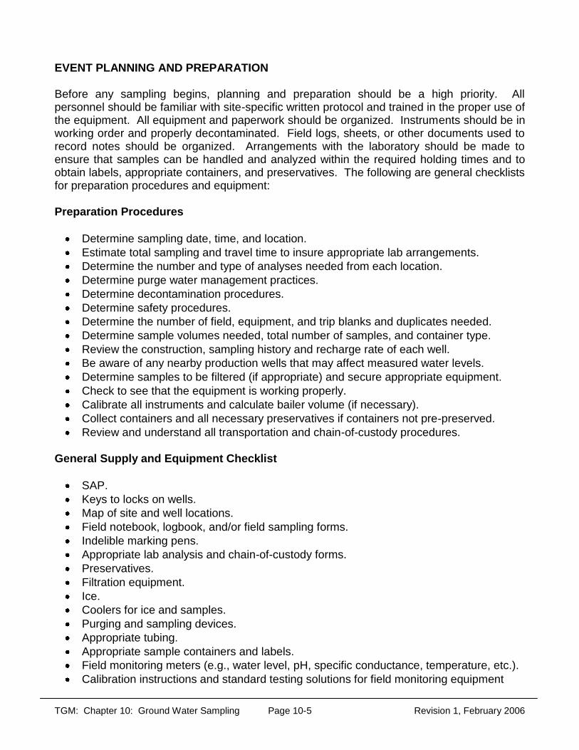
TGM: Chapter 10: Ground Water Sampling Page 10-5 Revision 1, February 2006
EVENT PLANNING AND PREPARATION Before any sampling begins, planning and preparation should be a high priority. All personnel should be familiar with site-specific written protocol and trained in the proper use of the equipment. All equipment and paperwork should be organized. Instruments should be in working order and properly decontaminated. Field logs, sheets, or other documents used to record notes should be organized. Arrangements with the laboratory should be made to ensure that samples can be handled and analyzed within the required holding times and to obtain labels, appropriate containers, and preservatives. The following are general checklists for preparation procedures and equipment: Preparation Procedures
Determine sampling date, time, and location. Estimate total sampling and travel time to insure appropriate lab arrangements. Determine the number and type of analyses needed from each location. Determine purge water management practices. Determine decontamination procedures. Determine safety procedures. Determine the number of field, equipment, and trip blanks and duplicates needed. Determine sample volumes needed, total number of samples, and container type. Review the construction, sampling history and recharge rate of each well. Be aware of any nearby production wells that may affect measured water levels. Determine samples to be filtered (if appropriate) and secure appropriate equipment. Check to see that the equipment is working properly. Calibrate all instruments and calculate bailer volume (if necessary). Collect containers and all necessary preservatives if containers not pre-preserved. Review and understand all transportation and chain-of-custody procedures.
General Supply and Equipment Checklist
SAP. Keys to locks on wells. Map of site and well locations. Field notebook, logbook, and/or field sampling forms. Indelible marking pens. Appropriate lab analysis and chain-of-custody forms. Preservatives. Filtration equipment. Ice. Coolers for ice and samples. Purging and sampling devices. Appropriate tubing. Appropriate sample containers and labels. Field monitoring meters (e.g., water level, pH, specific conductance, temperature, etc.). Calibration instructions and standard testing solutions for field monitoring equipment

TGM: Chapter 10: Ground Water Sampling Page 10-6 Revision 1, February 2006
Calibrated bucket (to determine volume of purged water). Tool box. Extra batteries. Safety equipment. Calculator. Plastic sheeting for ground cover. Decontamination solutions and equipment. Flashlight. Photoionization detector (PID) or organic vapor analyzer (OVA). Equipment for detecting immiscibles (e.g., interface probe or clear bailer). Contact information for site, facility, and laboratory. Emergency contact information.
PARAMETER SELECTION Parameter selection depends on whether the purpose of sampling is to quantify the general quality of the ground water or identify the presence of any contamination. Parameters to Characterize General Quality Parameters used to characterize general quality can include: pH, alkalinity, total dissolved solids (TDS), turbidity, dissolved oxygen, oxidation/ reduction potential (ORP), fluoride (F-), hydrogen sulfide (H2S), total hardness and non-carbonate hardness, specific conductance, chloride (Cl-1), nitrate (NO3
-1), sulfate (SO4-2), phosphate (PO4
-3), silicate (SiO2), sodium (Na+1), potassium (K+1), calcium (Ca+2), magnesium (Mg+2), ammonium (NH4
+1), total iron (Fe), and manganese (Mn). The results can provide an overall picture of ground water geochemistry that is useful to site characterization. For example, an understanding of geochemistry can help in determining chemical species present (e.g., AsO3
-2 versus AsO4-3)
and mobility in the subsurface. Certain parameters (e.g., anions, cations, pH, TDS, specific conductance) are helpful in evaluating releases of inorganic contaminants, while other parameters (chloride, iron, nitrate, sulfate, dissolved oxygen, ORP, and alkalinity) can be used to evaluate changes in ground water chemistry caused by the release and biodegradation of organic contaminants. Regulated entities (such as municipal or hazardous waste landfills) may be required to establish a sampling program that may include some the above-mentioned parameters. Parameters to Characterize Contamination When ground water contamination is known, suspected, or being investigated as part of a monitoring program, parameters specific to the waste material, history of the site/facility, or chemicals of concern (COCs) usually are necessary. Rules may also dictate specific parameters. When ground water contamination is known or suspected, entities may be required to monitor additional site-specific parameters4.
4 It is suggested that, in some cases (e.g., characterizing known ground water contamination), that the laboratory be requested to report all constituents listed in a methods target analyte list whether they are detected or quantified or not. This ensures that breakdown products are also considered.

TGM: Chapter 10: Ground Water Sampling Page 10-7 Revision 1, February 2006
Past waste constituents and handling practices should be considered. Because waste released to the environment may chemically change through time, potential breakdown products should be considered. If accurate disposal records are available and waste constituents are well documented, the list of parameters can be relatively limited. The list should be more extensive if handling practices are poorly understood. Monitoring suites of parameters (e.g., volatiles, semi-volatiles, metals, etc.) may be necessary when specific waste constituents are not known. Where rule/policy allows, lists may be narrowed as the investigation progresses and waste constituents and chemicals of concern become better defined.
SAMPLING AND PURGING EQUIPMENT A variety of sampling and purging equipment is available. Depending on the situation, all types have advantages and disadvantages. There is no device that can be used in every situation. Site-specific hydrogeology, geochemistry, types of contaminants, and well design may affect equipment performance. Ultimately, the ideal scheme should employ inert material, should not subject samples to negative pressures or high positive pressures, and should minimize exposure of samples to the atmosphere (ASTM, Method D4448-01). CRITERIA FOR SELECTION In general, the choice of a device should be based on the characteristics of the device in combination with the characteristics of the site/project. The following paragraphs discuss these characteristics and the criteria that should be considered. Device Characteristics Characteristics of devices are: • Device composition - The chosen device should have sample-contacting parts made of
"inert" materials that limit the potential for bias through sorption or leaching of contaminants, degradation, or corrosion. For components requiring rigid material (casing, screen, bailers etc.), the acceptable materials are fluorocarbon polymer (e.g., Teflon®), stainless steel (316 and 304), and PVC. Disposable bailers can also be composed of polyethylene and polypropylene. When sampling for organics, pump tubing should be composed of flurocarbon polymer, or flurocarbon polymer-lined polyethene. Polyethene tubing is also acceptable for sampling for inorganics (U.S.G.S, U.S.EPA, 2002, ASTM 4088).
• Device design and technique of use - The device should deliver samples with minimal
atmospheric exposure, should not apply negative pressures (vacuum), and should limit agitation, both in the well and in the transfer process. Furthermore, the tool should not introduce air or non-inert gas into samples as part of its lift mechanism.
• Flow rate control and capacity - When pumps are used, low flow rates are desirable to
limit agitation and turbulent flow, especially for VOCs (Barcelona et al., 1985, U.S. EPA, 1986a). The ability to maintain a steady low flow varies significantly. If the device is

TGM: Chapter 10: Ground Water Sampling Page 10-8 Revision 1, February 2006
being used for purging and sampling, then it should be capable of being operated at variable flow rates suitable for both applications. Flow control that involves "valving" should be avoided, since it can cause pressure changes and subsequent sample alteration. Instead, a mechanism that directly controls the rate (i.e., a rheostat to vary the power supplied to an electric submersible pump) should be utilized.
• Operation and Maintenance - The device should be easy to operate and maintain. If
personnel are not properly trained, the margin of potential error is greater. The device should be designed for in-field maintenance. Mechanically simple equipment that can be easily repaired with inexpensive, replaceable parts is preferable. If decontamination is necessary, the device should be easy to decontaminate. Devices that are constructed to minimize the surface area contacting ground water samples and that are easy to disassemble and reassemble are best. Use of dedicated or disposable equipment at each well or sampling point eliminates the need for decontamination, saving valuable field time and reducing the potential for cross contamination of samples.
• Device reliability, durability, and portability - The device should operate reliably for
extended periods and be able to withstand a variety of chemical and physical environments. Dedicated equipment may need to withstand extended contact with ground water and any existing contamination. Equipment that is transported into locations where access is limited should be sufficiently portable. Excess weight and volume of battery packs, generators, air compressors, tubing, etc. can limit portability.
• Capital, operation, and maintenance costs - These should be considered, however,
they should not be overriding factors. Obtaining a sample that is representative of site conditions should be of more importance than cost, particularly when the costs of well installation, chemical analysis, and possible litigation resulting from discrepant analytical results are considered. These costs often far outweigh equipment purchase costs (Nielsen and Yeates, 1985).
Site/Project Characteristics Characteristics of sites/projects that should be considered are:
• Monitoring Well Diameter - The device should be compatible with the diameter of the well. Most sampling equipment is not designed to be used in all wells.
• Well Obstructions or Constrictions - These can hinder the entry and retrieval of
sampling equipment. For example, casing joints may not be flush and could prevent insertion. Also, a well that is not plumb can restrict access.
• Depth to the Sampling Interval - Deeper zones require greater lift capacity and
generally increase sampling times, which may limit the desirability of labor-intensive devices. Options generally become limited as depth increases.
• Parameters of Interest - The suitability of various devices may depend on the
parameters of greatest concern. Some devices perform better for inorganics, while some are more suitable for VOCs.

TGM: Chapter 10: Ground Water Sampling Page 10-9 Revision 1, February 2006
• Presence of Non-Aqueous Phase Liquids (NAPLs) - The equipment should be capable of detecting the presence of either light or dense NAPLS if they are potentially present.
• Saturated Zone Characteristics and Ground Water Chemistry - The equipment
should be appropriate for the saturated zone yield, the screen or open borehole length, the presence of stratification (causing vertical variation in yield) within the screened saturated zones, and the available water column in the well. Additionally, the sampling equipment should be compatible with ambient ground water chemistry, unusually low (<5.5.U.) or high (>9.5.U.) pH conditions, the presence of gas, etc.
• Temporal (Seasonal) Variations - The sampling equipment should be operable over
seasonal variations in saturated zone temperature, yield and water level elevation. TYPES OF EQUIPMENT The following is a discussion of some of the sampling equipment available. Table 10.3 (at the end of this section) summarizes the recommended devices. Devices not mentioned may be acceptable if they are peer-reviewed and have been demonstrated to be capable of collecting representative samples. For additional information, see ASTM D4448-01, ASTM D6634-01, Barcelona et al. (1985), Nielsen and Yeates (1985), Electric Power Research Institute (EPRI, 1985, 1987), Gillham et al. (1983), Nielsen and Nielsen (2006), Parker (1994), Pohlman and Hess (1988), and U.S. EPA (1992), Yeskis and Zavala (2001). Grab Samplers Grab samplers collect a sample at discrete depths without being pumped or lifted to the surface by gas or air. Grab samplers commonly used to collect ground water include bailers and syringe samplers. Bailers Bailers are the most portable of all sampling devices. A bailer can be constructed of virtually any rigid or flexible material, including materials that are inert to chemical contaminants. For sampling ground water, acceptable compositions include Teflon®, stainless steel, PVC, polyethylene, and polyprolyene. Disposable bailers are often the choice of the environmental industry. The cord used to raise and lower the bailer should be of non-reactive substance (e.g., stainless steel, teflon-coated wire/rope, polypropylene). Bailers are readily available in a variety of diameters. Their diameter should be 75% (or less) of the inside diameter of the well casing to allow for adequate clearance. There are several types of bailers (ASTM D 6634-01, D6699-01):
A top filling bailer is designed such that water flows through its top. Because of the agitation of the sample, this bailer is only appropriate for sampling light, non-aqueous phase liquids (LNAPL).

TGM: Chapter 10: Ground Water Sampling Page 10-10 Revision 1, February 2006
A single check valve bailer (open bailer) has a valve at its bottom that seals the sample chamber when the bailer is withdrawn.
A double check valve bailer (point source bailer) is designed to sample discrete zones
in a water column. Water flows through valves at both ends as the bailer is lowered. When the desired level is reached, the bailer is pulled back, both valves close, and water from the interval is retained. However, if appropriate procedures are not carefully followed, samples collected may not be representative of the depth interval of interest. The double check valve bailer is also effective in collecting dense, non-aqueous phase liquids (DNAPLs).
A differential pressure bailer consists of a sealed canister body with two small diameter tubes of different heights. The bailer is rapidly lowered into the well. When the descent has stopped, differences in hydrostatic pressure between the two tubes allow the bailer to fill through the lower tube as air is displaced through the upper tube. This minimizes the exposure of the sample to air, especially if the bailer is fitted with internal 40 ML vials for direct sample bottle filling. However, because the bailer is lowered rapidly, it will agitate the water column.
The use of bailers is discouraged. Current research indicates that bailers generally are not the best available technology to collect ground water samples. Various studies (laboratory and field) have been conducted to investigate the potential differences in VOC analytical results between samples collected by bailing and low-flow techniques. Some studies have demonstrated that levels of VOCs in samples obtained with bailers are statistically lower than in samples obtained with other devices (Imbrigiotta et al. 1988; Tai et al. 1991). In addition, bailing can cause increased turbidity (Puls and Powell, 1992; Puls et al., 1992; Backhus et al., 1993). In contrast, a literature survey by Parker (1994) found that bailers can recover representative samples under certain circumstances and that loss of volatile and oxidizable analytes can be reduced by careful use of bottom-emptying devices. In addition, a Wisconsin Department of Natural Resources study comparing results from a bottom-emptying bailer and a Keck® helical-rotor pump operated at low flow pumping rates determined that differences in VOC concentrations were relatively small (Karkins, 1996). Though current research indicates that bailers generally are not the best available technology, they may be the only practicable option for sampling some ground water zones. Bailers may be preferred where the water column is small or the saturated zone is very deep. They may be preferred when concentrations of contaminants are extremely high because they are easier to decontaminate and are less expensive to replace than pumps. Disposable bailers eliminate the need to decontaminate. Personnel sampling with bailers need to be properly trained since the results are highly dependent on the skill, care, and consistency of the operator. This training should be documented in the SAP. If bailers are used, double check valve bottom-draining bailers are recommended. This allows for lessened sample disturbance during transfer to the container. The bailer should be composed of Teflon®, stainless steel, PVC, polyethylene, or polyprolyene. Either fluorocarbon polymer-coated or colorless (white) polypropylene cord should be used to lower and raise the bailer. Polypropylene cord is inexpensive enough to be discarded after one use. A bailer should always be lowered and raised slowly to minimize sample agitation

TGM: Chapter 10: Ground Water Sampling Page 10-11 Revision 1, February 2006
associated with degassing, aeration, and turbidity and to the extent possible, avoid hitting the sides of the well. A tripod and pulley may be used to remove the bailer. Pouring water from the top of a bailer either directly into a container or to a transfer vessel may agitate/aerate the sample and alter its chemistry; therefore, the pouring should be done with care. Syringe Samplers Syringe samplers may be used for low-volume sampling for inorganics and non-volatile organics. These samplers can operate at great depths to provide discrete samples from specific intervals or zones. A sample container is pressured or evacuated and lowered into a well. The sample is collected by opening the container or releasing the pressure, drawing water into the sampler (Nielsen and Nielsen, 2006). The syringe sampler is withdrawn and the sample is transferred to a collection bottle, or alternatively, the syringe sampler can be utilized as the sample container. Syringe devices cannot be used for purging large volumes and are ineffective for collecting large samples. In addition, ground water containing high concentrations of suspended solids may cause the syringe device to leak (U.S. EPA, 1992). Researchers have concluded that these samplers are inferior in comparison to other devices when sampling for VOCs (lmbrigiotta et al., 1988). Therefore, syringe samplers are not recommended. Bladder Pumps A bladder pump consists of a flexible bladder inside a rigid housing. Water enters the bladder from the bottom and is squeezed to the surface through a discharge line by gas pressure applied to the outside of the bladder. An air compressor and regulator turn the pressure on and off, allowing new water to enter the bladder and the cycle is repeated. The separate bladder chamber does not allow the sample to come in contact with the compressed air. Check valves at the top and bottom prevent backwash from the sample tube and bladder. Flow can be readily controlled and low rates of 100 ml/min are easily obtainable. Teflon bladders and Teflon/stainless steel outer shells are readily available and recommended. Bladder pumps have been used to depths greater than 200 feet and are available in sizes designed for 2-inch wells. The need for a power source and compressed air limits mobility, especially in remote areas. Potential problems include sediment damaging the inner bladder and high suspended solids concentrations causing failure of check valves for some models (Nielsen and Nielsen 2006). Strainers or screens are available that attach below the bladder to filter material. Note that samples collected through a strainer or screens are not considered to be filtered. Bladder pumps are generally recognized as the best overall sampling device for both inorganic and organic constituents (U.S. EPA, 1992). Muska et al., (1986) found that bladder pumps generate reproducible analytical results. Kasper and Serkowski (1988) concluded that the sampling rate and reliability of the bladder pump outperformed both the gas and mechanically driven piston pumps. Tai et al. (1991) concluded that a bladder pump yielded

TGM: Chapter 10: Ground Water Sampling Page 10-12 Revision 1, February 2006
representative recoveries of VOCs compared to a control sample. Pohlmann and Hess (1988) determined that bladder pumps are suitable for collecting samples for almost any constituent. Bladder pumps are recommended for purging and sampling. Whenever possible, the pump should be dedicated to the well. Doing so eliminates the need to transport and decontaminate the pump, thereby reducing the potential for cross contamination as well as saving time and reducing project cost. Electrical Submersible Pumps A variety of electrical submersible pumps are available. In the past, electrical submersible pumps were primarily designed for use in water supply wells and could not be used for contaminant monitoring purposes. However, manufacturers have since designed low-flow electrical submersible pumps for 2-inch diameter monitoring wells that are capable of collecting representative samples. Submersible pumps designed for ground water sampling incorporate non-sorptive materials (e.g., stainless steel, Teflon®, etc.) that are appropriate for collecting VOCs and other sensitive parameters. One disadvantage is that the heat generated by the motor could increase sample temperature, resulting in the loss of dissolved gases and VOCs and subsequent precipitation of trace metals (Nielsen and Nielsen, 2006) Therefore, after sampling, it is recommended that a sample be withdrawn and the temperature measured to assess whether the pump has increased the water temperature. Another disadvantage is the number of intricate parts, which may cause decontamination and maintenance to be time-consuming and difficult. Two types of submersible pumps available are the centrifugal and the progressive cavity (helical-rotor) pumps. Both are positive displacement devices. Centrifugal Submersible Pump Centrifugal submersible pumps designed for 2-inch monitoring wells are usually cooled and lubricated with water rather than hydrocarbon-based coolants and lubricants that could contaminate samples. The electric motor spins or rotates an impeller (or series of impellers) that causes water to be accelerated outward and then upward into and through the pump’s discharge lines. The higher the pumping rate, the greater the potential for sample alteration by agitation, increased turbulence, and pressure changes. Therefore, a variable-speed centrifugal submersible pump capable of low-flow purging and sampling is essential for collecting a representative sample. Low-flow centrifugal submersible pumps appear to perform similarly to low-flow bladder pumps with respect to preserving sample integrity. Progressive Cavity (Helical-Rotor) Pumps Progressive cavity (helical-rotor) pumps are appropriate for collecting sensitive samples if low-flow pumping rates are used. An electric motor at the base turns a corkscrew-like helical rotor near the top. The helical rotor causes an upward movement of water trapped in the vacuities of the rotor and the water moves up and through the discharge line. A check valve at the top ensures that water in the discharge line (sampling tube) does not re-enter the pump. A controller box at the surface allows for variable flow rates.
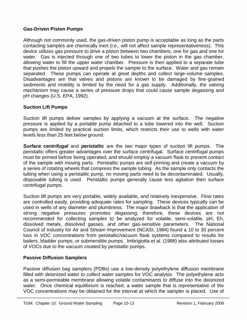
TGM: Chapter 10: Ground Water Sampling Page 10-13 Revision 1, February 2006
Gas-Driven Piston Pumps Although not commonly used, the gas-driven piston pump is acceptable as long as the parts contacting samples are chemically inert (i.e., will not affect sample representativeness). This device utilizes gas pressure to drive a piston between two chambers, one for gas and one for water. Gas is injected through one of two tubes to lower the piston in the gas chamber, allowing water to fill the upper water chamber. Pressure is then applied to a separate tube that pushes the piston upward and propels the sample to the surface. Water and gas remain separated. These pumps can operate at great depths and collect large-volume samples. Disadvantages are that valves and pistons are known to be damaged by fine-grained sediments and mobility is limited by the need for a gas supply. Additionally, the valving mechanism may cause a series of pressure drops that could cause sample degassing and pH changes (U.S. EPA, 1992). Suction Lift Pumps Suction lift pumps deliver samples by applying a vacuum at the surface. The negative pressure is applied by a portable pump attached to a tube lowered into the well. Suction pumps are limited by practical suction limits, which restricts their use to wells with water levels less than 25 feet below ground. Surface centrifugal and peristaltic are the two major types of suction lift pumps. The peristaltic offers greater advantages over the surface centrifugal. Surface centrifugal pumps must be primed before being operated, and should employ a vacuum flask to prevent contact of the sample with moving parts. Peristaltic pumps are self-priming and create a vacuum by a series of rotating wheels that compress the sample tubing. As the sample only contacts the tubing when using a peristaltic pump, no moving parts need to be decontaminated. Usually, disposable tubing is used. Peristaltic pumps generally cause less agitation then surface centrifugal pumps. Suction lift pumps are very portable, widely available, and relatively inexpensive. Flow rates are controlled easily, providing adequate rates for sampling. These devices typically can be used in wells of any diameter and plumbness. The major drawback is that the application of strong negative pressures promotes degassing; therefore, these devices are not recommended for collecting samples to be analyzed for volatile, semi-volatile, pH, Eh, dissolved metals, dissolved gasses, and other gas-sensitive parameters. The National Council of Industry for Air and Stream Improvement (NCASI, 1984) found a 10 to 30 percent loss in VOC concentrations from peristaltic/vacuum flask systems compared to results for bailers, bladder pumps, or submersible pumps. Imbrigiotta et al. (1988) also attributed losses of VOCs due to the vacuum created by peristaltic pumps. Passive Diffusion Samplers Passive diffusion bag samplers (PDBs) use a low-density polyethylene diffusion membrane filled with deionized water to collect water samples for VOC analysis. The polyethylene acts as a semi-permeable membrane allowing volatile contaminants to diffuse into the deionized water. Once chemical equilibrium is reached, a water sample that is representative of the VOC concentrations may be obtained for the interval at which the sampler is placed. Use of

TGM: Chapter 10: Ground Water Sampling Page 10-14 Revision 1, February 2006
multiple PDB samplers at different depths within a well screen interval can allow for a vertical profile of the VOC contamination within the well. Advantages of PDB sampling include its low cost, minimal purging and water disposal, and the ability to monitor a variety of VOCs. A disadvantage is that they are not applicable to inorganics and other contaminants that do not readily diffuse across the semi-permeable membrane. PDB sampling may not be applicable for sites where water in the well casing may not be representative of the saturated zone adjacent to the well screen. This may occur when water in the well casing is stagnant, or when there is a vertical flow within the well. In addition, PDB samplers do not provide a discrete time-interval sample, but rather an average of the concentrations in the well over the equilibrium period. Passive diffusion bag samplers are appropriate for long-term monitoring at well-characterized sites. The target analytes should be limited to chemicals that have been demonstrated to diffuse well through polyethylene (i.e., most VOCs and limited non-VOCs), as listed in Tables 1-1 and 4-1 of ITRC’s PDB sampler guidance document (ITRC, 2004). A combined version of these tables is provided below as a reference (Table 10.2). However, as the compound list may change as further tests are conducted, ITRC (http://www.itrcweb.org) should be contacted for the most recent list of chemicals favorable for sampling with PDB. The site sampled should have sufficient ground water flow to provide equilibrium between the water in the well screen and the surrounding ground water zone. ITRC (2004) suggests that care should be given in interpreting PDB results when the hydraulic conductivity is <10-5 cm/s, the hydraulic gradient is <0.001, or the ground water velocity is < 0.5 ft/day. Use of PDBs is not appropriate when a vertical flow in the well exists. A deployment time of at least two weeks is recommended to allow for diffusion of the analytes across the membrane (ITRC, 2004, Vroblesky, 2001; Vroblesky and Hyde, 1997; Yeskis and Zavala, 2001; and U.S.G.S , 2002). Other Devices The gas drive sampler operates by applying positive gas pressure into a sample chamber to force the water to the ground surface. Water enters through a valve at the bottom of the sampler into the sample chamber. When pressure is applied, the valve closes and water is forced through a discharge line to the surface. When the pressure is reduced, the valve reopens, allowing water to enter the chamber, and the cycle is repeated. Gas drive samplers are available with inert components and in a variety of diameters. They can provide continuous flow at acceptable rates for sampling. Their major drawback is that they allow for gas contact with the sample, which can cause the loss of dissolved gasses and VOCs and potentially other chemical alterations. Gas can also mix with the sample, causing further alteration. For these reasons, use of these samplers is generally not recommended. Additionally, mobility is limited by the need to provide compressed gas. When sampling very deep wells, high gas pressures are needed, and the device should be designed to handle this added stress. Gas lift samplers inject air or gas into the water column to "blow" water to the surface. The gas acts as a carrier fluid; however, the gas (even if inert) causes degassing and volatilization. Additionally, aeration and turbulence can further alter the original water chemistry (Lee and Jones, 1983). Therefore, gas lift systems are unacceptable.

TGM: Chapter 10: Ground Water Sampling Page 10-15 Revision 1, February 2006
Table 10.2 Compounds tested with PDB in laboratory and field tests.
Favorable laboratory diffusion testing results
Benzene Bromodichloromethane* Bromobenzene** Bromochloromethane** Bromoform* n-Butylbenzene** sec-Butylbenzene** tert-Butylbenzene** Carbon disulfide** Carbon tetrachloride Chlorobenzene Choroethane Chloroform* Chloromethane 2-Chlorovinylether* Dibromochloromethane Dibromomethane 1,2-Dichlorobenzene
1,3-Dichlorobenzene 1,4-Dichlorobenzene Dichlorodifluoromethane 1,1-Dichchloroethane** 1,2-Dichloroethane 1,1-Dichloroethene cis-1,2-Dichloroethene trans-1,2-Dichloroethene 1,2-Dichloropropane cis-Dichloropropene* 1,2-Dibromoethane* trans-1,3-Dichloropropene* Ethyl benzene Hexachlorobutadiene** p-Isopropyltoluene** 1-Methylethylbenzene**
Napthalene* 1,1,2,2-Tetrachloroethane Tetrachloroethene (PCE) Toluene 1,2,3-Thrichlorobenzene** 1,2,4-Trichlorobenzene** 1,1,1-Trichloroethane 1,1,2-Trichloroethane Tricholoroethene (TCE) Trichlorofluoromethane 1,1,2-Trhichloro-1,2,2-trifluoroethane** 1,2,3-Trichloropropane* Vinyl chloride m,p-Xylene** o-Xylene** Xylenes (total)
Unfavorable diffusion testing results
Acetone* tert-Amyl methyl ether**# Bromoform**# Methyl iso-butyl ketone*
Methyl tert-butyl ether* Naphthalene** n-Propylbenzene**
Styrene* 1,2,4-Trimethylbenzene** 1,3,5-Trimethylbenzene**
* Laboratory results only, (Vroblesky 2001a) **Results from field tests only, (Parsons 2003) #The data set for this compound was relatively small (fewer than five instances of comparison), so the power of the classification (i.e., acceptable or unacceptable) is fairly low. Use of Packers Packers are inflatable rubber devices used in a well or open borehole to isolate water-bearing intervals for hydraulic testing or ground water sampling. Packers can be used to minimize purge volumes in wells with long intake columns by isolating the sampled zone from stagnant water above the screen. Both single and double packer assemblies are used. For sampling, a pump is typically installed above or below a single packer or within a double packer assembly with a discharge line extending through the upper packer. Packer assemblies may include a drop tube through which water level tapes, transducers, pump control and discharge lines, and other monitoring and sampling equipment may extend to the isolated interval. Prior to using packer assemblies for sampling, all potential limitations or problems should be carefully evaluated and resolved, and the use of packers should be justified. For example, packer materials selected should not leach or sorb contaminants. In addition, the water level within the packer interval should not be drawn down below the upper packer. The potential for vertical movement of ground water to or from the packer interval outside of the well or borehole should be evaluated, as well as the potential for leakage around the inflated packers. For additional discussion on packers, refer to Oliveros et al.(1988).

TGM: Chapter 10: Ground Water Sampling Page 10-16 Revision 1, February 2006
Table 10.3 Summary of recommendations for sampling mechanisms5.
MECHANISM
RECOMMENDATIONS
POTENTIAL FOR CHEMICAL ALTERNATION*
COMMENTS
Bailer
Double check valve bailers with bottom emptying device Can be used for sampling organics and inorganics.
slight to
moderate
Samples may show statistically lower analytical results. Other techniques may be more appropriate when low levels of organics exist.
Bladder pump
Highly recommended. Can be used for sampling organics and inorganics
minimum to slight
Provides efficient well purging and representative samples over a range of conditions.
Electric Submersible
Pumps
Pumps should be constructed of inert components and capable of sampling at low flow rates. Can be used to sample organics and inorganics.
slight to moderate
Good for purging and sampling deep, high yielding wells. Recommend monitoring temperature, to assure pumping does not increase sample temperature.
Gas Driven
Piston Pumps
Acceptable if sample compositions are met. Can be used to sample organics and inorganics.
slight to
moderate
Difficult to decontaminate.
Syringe Sampler
Recommended for low volume sampling of discrete zones. Can be used for sampling inorganics and non-volatile organics, not recommended when sampling for volatiles.
minimum to slight
Cannot be used for purging.
Suction Lift Pumps (Peristaltic/ Centrifugal)
Not recommended for sampling for volatiles and semi-volatiles
moderate to high Can cause significantly lower recoveries of purgeable organic compounds and gases.
Passive Diffusion Bag Samplers (PDB samplers)
Long-term monitoring of VOCs at sites with sufficient ground water flow. Cannot be used for inorganics or most non-VOCs
slight Sampler does not provide a discrete time-interval sample, but instead an average concentration over the equilibration period Not appropriate if chemicals of concern are transported on suspended particles Not acceptable for inorganics or phthalates.
5Table does not address gas drive and gas lift samplers. These devices generally are not recommended.
TGM: Chapter 10: Ground Water Sampling Page 10-17 Revision 1, February 2006
FIELD PROCEDURES
As appropriate, the health and safety plan should be reviewed prior to initiating field procedures. Sampling personnel should not use perfume, hand lotion etc. when collecting a ground water sample. If insect repellent is necessary, then care should be taken not to allow the repellent to come into contact with the sampling equipment and it should be recorded that insect repellent was used (Wilson, 1995). Activities that may affect sampling, such as fueling a vehicle, should be avoided. Prior to sampling, several tasks should be completed and documented to ensure that representative samples can be obtained. These tasks include, but are not limited to: observation of field conditions, well inspection and preparation, well measurements, and immiscible layer detection. (Documentation guidance is provided in subsequent parts of this chapter). FIELD CONDITIONS Weather and site-specific conditions that could affect sample representativeness should be documented. The approximate ambient air temperature, precipitation, and wind and other field conditions should be noted in a field notebook or field sampling form. In addition, any site-specific conditions or situations that could potentially alter the ground water samples or water level measurements should be recorded. Examples include, but should not be limited to: excavation or construction activities, accidental spills, and presence of smoke, vapors, or air contaminants from anthropogenic activities. WELL INSPECTION AND PREPARATION Upon arrival, the well protective casing, cap, and lock should be carefully inspected and observations recorded to document whether damage or tampering has occurred.6 Cracks in the casing and/or surface cement seal should be noted, as well as soil washouts and depressions around the casing. Before taking any measurements, all weeds and debris should be cleaned from the well area. All equipment should be covered and stored off the ground to avoid potential cross-contamination. A clean plastic sheet can be placed on the ground to help prevent contamination of equipment if there is a concern that sample equipment may come into contact with the ground. The plastic should be disposed properly following completion of sampling at each well. A portable field table covered with a new plastic sheet at each well is convenient for preparing equipment and performing field measurements (Wilson, 1995).
6 See Chapter 8 (Well Development, Maintenance, and Redevelopment) for additional information on periodic well maintenance checks and well-integrity tests).

TGM: Chapter 10: Ground Water Sampling Page 10-18 Revision 1, February 2006
WELL MEASUREMENTS Appropriate measurements should be made before any water is purged and sampled. These include measuring of static water levels and total well depth, and depending on site-specific conditions or circumstances, detection of gases, organic vapors and immiscible liquids. Detection of Organic Vapors and Gases Because VOCs often present health and safety concerns, it may be prudent to use field screening instruments if VOCs are suspected. Two field screening instruments that may be useful are the photoionization detector (PID) and an organic vapor analyzer (OVA).7 PIDs and OVAs are typically used to provide an estimate of the total volatile organic vapor concentration (e.g., benzene, vinyl chloride, tetrachloroethane), rather than a quantitative result for individual compounds. OVAs are capable of detecting methane, while PIDs are not. The selection of the correct lamp is important when using a PID meter. Field meters are available for detecting methane, carbon dioxide, and hydrogen sulfide, including combination meters that can be used to screen for two or more of these gases. Vapor measurements can give useful information about potential ground water quality and allow for sampling personnel to take appropriate safety precautions. It also may be useful to determine the potential for the presence of immiscible layers, which necessitate additional sampling procedures and concerns. Gases that typically may be of concern include methane, carbon dioxide, and hydrogen sulfide. Generally, methane and carbon dioxide may occur in monitoring wells at solid waste landfill facilities. Methane may also be present as natural gas in bedrock formations. The presence of methane is significant because it may include trace amounts of VOCs that are too low to be detected with a PID or OVA. Additionally, methane is a health and safety concern because it can cause a potentially explosive atmosphere. Carbon dioxide may affect ground water chemistry by altering pH or alkalinity. Hydrogen sulfide, which is typically associated with sewage or decaying vegetation, may affect pH meter performance. Hydrogen sulfide gas can also be naturally occurring in carbonate bedrock aquifers. Water Level In addition to providing hydrogeologic information on a continuing basis, measurement of the water level in a well enables determination of the volume of water contained, which may be useful for purging determinations. Measurements should be taken from the entire well network before any water removal to obtain a single "snapshot" of current hydraulic head conditions and to avoid potential effects on the water levels in nearby wells. The measurements should be made within a period of time short enough to avoid temporal variations in ground water flow that could preclude an accurate determination of ground water flow rate and direction. The period of time should not exceed 24 hours. Measurements can be taken manually or automatically. Table 10.4 summarizes the manual methods. Automatic, continuous recording devices may be useful for collection of long-term
7For further information on types and uses of these instruments, see Anastas and Belknap (1980), Brown et al. (1980) and DuBose et al. (1981).

TGM: Chapter 10: Ground Water Sampling Page 10-19 Revision 1, February 2006
data and in pumping tests. Water level measurements are described in more detail by Dalton et al. (1991), Aller et al. (1991), and ASTM Method D4750-87. An electronic probe is recommended for taking water level measurements. Measurements should generally be to within ±0.01 ft. There may be instances where this level of accuracy is not necessary (e.g., steep water table, wells are far apart); however, rules may require this level of accuracy. All wells should have accurate surveyed reference points8 for water level determination. Typically, a marked point on the top of the inner riser pipe is used. Equipment should be properly decontaminated before use in each well to ensure sample integrity and prevent cross-contamination. Techniques are discussed later in this chapter. Light non-aqueous phase liquid (LNAPL) (see below) may affect the water level measurements in a well. It is important to know the density of the free product because water level measurements in monitoring wells that also contain free product should be corrected to account for the different densities of water and product and the thickness of the product layer. See U.S. EPA (1996a) for procedure to correct for an LNAPL layer. Well Depth Measuring the depth of a well indicates the amount of siltation that has occurred. Natural siltation can block water from entering, which could lead to erroneous water level measurements and bias analytical results by increasing sample turbidity. Checking depth also provides a check on casing integrity. Corrosion can cause collapse of the well casing. Depth can be determined with a weighted tape measure or marked cable, each of which should be composed of inert materials. Often, the same device that is used to measure water levels can be used. Heavier weights are necessary as depth increases to effectively "feel" the well bottom. The measurement should be recorded on the field log. It generally is not necessary to measure depth every time water levels or samples are obtained. It may not be possible to obtain depth from a well with a dedicated pump unless the pump is removed. In addition, the logistics of decontaminating the entire length of the measuring tape in contact with contaminated ground water may cause depth measurements to be impractical. At minimum, depth measurements should be taken once a year in wells that do not have dedicated pumps. Measurements in wells with pumps should be taken whenever the pump is removed for maintenance. If siltation is suspected to be a problem (e.g., noted increase in sample turbidity, or decrease in pump efficiency), the pump should be removed and the well depth checked
8It is recommended, the reference point be based on the National Geodetic Vertical Daturm or local common datum. However, an arbitrary datum common to all wells in the monitoring network may be acceptable if necessary.

TGM: Chapter 10: Ground Water Sampling Page 10-20 Revision 1, February 2006
Table 10.4 Summary of methods for manual measurement of water levels (based on Dalton et al., 2006, ASTM D4750 and U.S.EPA, 2001).
MEASUREMENT
METHOD
MEASUREMENT ACCURACY
(in feet)
DESCRIPTION & ADVANTAGES
MAJOR INTERFERENCES OR DISADVANTAGES
NON-FLOWING WELLS
Weighted steel tape with chalk
0.01 The water level is determined by lowering a weighted steel tape with bottom 2-3 feet coated with carpenters chalk into the well. The water level is calculated by subtracting the submerged distance, as indicated by the lack of chalk color, from the reference point at the top of the well. More accurate than other methods. Recommended when gradient is less than 0.05 ft/ft (Yeskis and Zavala, 2002).
• Water on the side of the casing or cascading water may wet the tape above the actual water level and result in measurement error.
• Addition of foreign material to well (chalk). • Approximate depth to water may be unknown,
thus too short or too long a length of chalked tape may be lowered into the well.
• Submergence of a weight and tape may
temporarily cause a rise of liquid in a small diameter well.
• Not recommended if obtaining ground water
samples for water quality purposes
Air-line 0.25 A small straight tube (usually 0.375 inches in diameter), of accurately known length is installed in the well along with a pressure gauge and a fitting for an air source. A water level measurement is made when air is pumped into the tube and the pressure monitored.
• Less precise • Air-line or fittings can leak
Electrical method
0.01 to 0.1 An electronic probe is lowered into the well. When the probe comes into contact with water, a potential between the two dissimilar metals in the probe is measured at the surface on a millivolt meter.
• Errors result from changes in cable length as a function of use, temperature and depth
• Reliable contact may be difficult if LNAPLs are
present
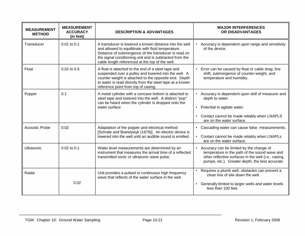
TGM: Chapter 10: Ground Water Sampling Page 10-21 Revision 1, February 2006
MEASUREMENT
METHOD
MEASUREMENT ACCURACY
(in feet)
DESCRIPTION & ADVANTAGES
MAJOR INTERFERENCES OR DISADVANTAGES
Transducer 0.01 to 0.1 A transducer is lowered a known distance into the well and allowed to equilibrate with fluid temperature. Distance of submergence of the transducer is read on the signal conditioning unit and is subtracted from the cable length referenced at the top of the well.
• Accuracy is dependent upon range and sensitivity of the device.
Float 0.02 to 0.5 A float is attached to the end of a steel tape and suspended over a pulley and lowered into the well. A counter weight is attached to the opposite end. Depth to water is read directly from the steel tape at a known reference point from top of casing.
• Error can be caused by float or cable drag, line shift, submergence of counter-weight, and temperature and humidity.
Popper 0.1 A metal cylinder with a concave bottom is attached to steel tape and lowered into the well. A distinct "pop" can be heard when the cylinder is dropped onto the water surface
• Accuracy is dependent upon skill of measurer and depth to water.
• Potential to agitate water. • Contact cannot be made reliably when LNAPLS
are on the water surface.
Acoustic Probe 0.02 Adaptation of the popper and electrical method [Schrale and Brandywyk (1979)]. An electric device is lowered into the well until an audible sound is emitted.
• Cascading water can cause false measurements. • Contact cannot be made reliably when LNAPLs
are on the water surface.
Ultrasonic 0.02 to 0.1 Water level measurements are determined by an instrument that measures the arrival time of a reflected transmitted sonic or ultrasonic wave pulse.
• Accuracy can be limited by the change of temperature in the path of the sound wave and other reflective surfaces in the well (i.e., casing, pumps, etc.). Greater depth, the less accurate.
Radar
0.02
Unit provides a pulsed or continuous high frequency wave that reflects of the water surface in the well.
• Requires a plumb well, obstacles can prevent a clean line of site down the well.
• Generally limited to larger wells and water levels
less than 100 feet.

TGM: Chapter 10: Ground Water Sampling Page 10-22 Revision 1, February 2006
MEASUREMENT
METHOD
MEASUREMENT ACCURACY
(in feet)
DESCRIPTION & ADVANTAGES
MAJOR INTERFERENCES OR DISADVANTAGES
Laser
0.01
Battery operated units potentially capable of obtaining water level information from monitoring wells.
• Further development is needed for adopting it to ground water monitoring programs
• Requires a plumb well, obstacles can prevent a
clean line of site down the well. • Beams can sometimes penetrate the water and
not reflect back
FLOWING WELLS
Casing Extension
0.1
A simple extension is attached to the well casing to allow water level to be measured directly.
• The device is only practical when additional height requirement is only several feet.
• Accuracy low because water level in flowing wells
tends to fluctuate.
Manometer/ Pressure Gauge
0.1 to 0.5
The pressure of water within a sealed or "shut-in" well is measured.
• Gauge inaccuracies. • Calibration is required.
Pressure Transducers
0.02
Procedures are the same as described above for transducers. The range of a pressure transducer should be carefully matched with shut-in well pressure.
• Changes in temperature in the transducers cause errors.
Depth measurements should be to the nearest 0.1 foot (U.S. EPA, 2001). Depth to bottom can be obtained when collecting the round of depth-to-water measurements. Care should be taken to avoid stirring up any accumulated sediments, thus increasing turbidity of the water column. If a well has historically had silting problems, consider taking the depth measurement after sampling.

TGM: Chapter 10: Ground Water Sampling Page 10-23 Revision 1, February 2006
Detection of Immiscible Liquids Non-aqueous phase liquids (NAPLs) are organic liquids that exist as a separate phase, immiscible phase when in contact with water and/or air. If the presence of NAPLs is suspected, the sampling program should include devices and protocols to detect them. Dense non-aqueous phase liquids (DNAPL) are referred to as "sinkers" because their density (greater than water) causes them to sink. Light non-aqueous phase liquids (LNAPL) are referred to as "floaters" because their density (less than water) causes them to float on the water table surface. If floaters are of concern, it is important that, upon opening the well cap, the air in the casing is monitored with a photoionization detector (PID) or an organic vapor analyzer (OVA). In addition to providing information on worker health risks, air monitoring can serve as a first indication of the presence of volatile floaters. Protocol to detect immiscible liquids should always include visual inspection of purged water and any equipment that is removed from the well after use. Additionally, probes and reactive pastes have been developed to determine air/immiscible and water/immiscible interfaces. Indicator pastes are used to coat an interface probe or a weighted tape. An observed reaction indicates the presence of an immiscible liquid. Probes and pastes can be utilized for detecting both floaters and sinkers (U.S. EPA, 1992). Transparent bailers also can be used. SAMPLING IMMISCIBLE LIQUIDS If an LNAPL is found to be present, a bailer or submersible pump can be used to remove it, if necessary (U.S. EPA, 1992). Any LNAPL greater than 2 feet in thickness can be evacuated using a bottom-valved bailer. The bailer should be lowered slowly to a depth less than the product/water interface. A modified, top-filling bailer (bottom valve sealed off with a fluorocarbon resin sheet between the ball and ball seat) can be used to remove immiscible layers less than 2 feet in thickness. A stainless steel weight can be added to the retrieval line above the bailer to counter its buoyancy. In either case, a peristaltic pump also can be utilized if depth to product is less than 25 feet. Any LNAPL less than 2 inches thick can be collected from the top of the water column using a bailer (U.S. EPA, 1992). Samples collected in this manner consist of both an aqueous and non-aqueous phase. To the extent possible, the sampling and purging method should prevent the disturbance of DNAPL. A sample of the DNAPL should be obtained after the ground water sample has been obtained. Double -check valve bailers, Kemmerer devices and syringe samplers often are used. Submersible pumps can be used if the dense phase is sufficiently thick (U.S. EPA, 1992). When an immiscible layer is to be analyzed, additional sampling equipment (i.e., containers) may be needed to have sufficient volume for laboratory analysis. It is important that appropriate QA/QC procedures be followed when collecting samples of any immiscible liquids. If any immiscible layer is removed, it should be properly collected, containerized, characterized, and managed. The Division of Hazardous Waste Management, Ohio EPA, can be contacted for guidance on these issues.

TGM: Chapter 10: Ground Water Sampling Page 10-24 Revision 1, February 2006
SAMPLING AND PURGING PROCEDURES Upon completion of the preliminary procedures, purging and sampling of ground water can generally be accomplished by volumetric or low flow rate methods. However, volumetric purging and low flow rate purging/sampling may not be feasible for wells that produce less than 100 ml/min. Therefore other approaches should be considered, including minimum/no purge sampling as well as purging to dryness and sampling as soon as the well has recharged sufficiently. These approaches are discussed below, along with methods to determine when purging is complete by measuring indicator parameters. Where dedicated equipment is not used, sampling should progress from wells least likely to be contaminated to those most likely to be contaminated to minimize the potential for cross-contamination. Care needs to be taken to avoid agitation and temperature increases in the sample during sample collection and shipment to the laboratory. Field Measurements of Ground Water Indicator Parameters Indicator parameters are measured in the field to evaluate well stabilization during purging, provide information on general ground water quality, help evaluate well construction, or indicate when well maintenance is needed. Indicator parameter data may be helpful in evaluating the presence of ground water contamination. Indicator parameters measured during well purging and sampling activities may include specific conductance, pH, dissolved oxygen, oxidation-reduction potential, temperature, and turbidity (Garner, 1988). Due to the unstable nature of these parameters, laboratory determinations will likely not be representative of field conditions, and consequently are of limited value. Specific conductance measures the ability of water to conduct an electric current. For ground water, it is generally reported in micromhos (mhos/cm), as natural waters commonly exhibit specific conductances well below 1 mhos/cm (Hem, 1992). Specific conductance is a relative measure of the amount of ions present in ground water, as the magnitude of the current conducted by a ground water sample is directly proportional to its ionic concentration. Based on this relationship, total dissolved solid concentrations may be approximated from specific conductance data (Hem, 1992). For most circumstances, specific conductance has been demonstrated to be a reliable indicator of the chemical stabilization of purge water (e.g., Barcelona et. al., 1994).9 High readings may indicate contamination, especially if the readings are elevated compared to background. Alternatively, elevated specific conductance may indicate grout contamination in a well or an inadequate grout seal, that is allowing infiltration of surface water or ground water from overlying saturated zones. Elevated specific conductance readings may also indicate inadequate well development (Garner, 1988).
pH is a measure of the effective concentration (or activity) of hydrogen ions and is expressed as the negative base-10 logarithm of the hydrogen-ion activity in moles per liter. Uncontaminated ground water typically exhibits a pH ranging from 5 to 9 (Brownlow, 1979;
9Specific conductance should not be used by itself to determine whether adequate purging has been completed. Ohio EPA recommends using multiple indicator parameters to determine when to terminate purging and begin sampling regardless of the assumed reliability of the data.

TGM: Chapter 10: Ground Water Sampling Page 10-25 Revision 1, February 2006
Ohio EPA, 2003). While pH has commonly been used as a purge water stabilization indicator, it is not particularly sensitive in distinguishing stagnant casing water from formation water. However, pH measurements are important for the interpretation of ground water quality data (Puls and Barcelona, 1996), as pH indicates the relative solubility of metals and speciation of many other chemicals (Garner, 1988). First, pH measurements reflect chemical reactions that produce or consume hydrogen ions (Hem, 1992), and therefore, changes in pH from background may indicate the presence of ground water contamination or that existing contamination has spread. Second, pH can be very useful in identifying well construction or maintenance problems. For example, pH readings that consistently increase in (7.8, 8.3, 8.8, 9.4...) during purging may indicate grout contamination in the sand pack and screened interval.
Dissolved oxygen (DO) has been demonstrated to be a reliable indicator of the chemical stabilization of purge water under most ground water purging and sampling circumstances (e.g., Barcelona et. al., 1994).1 DO is a good indicator when sampling for volatile organic compounds (VOCs), because erratic or elevated DO readings may reflect procedures that are causing excessive agitation and aeration of the ground water being drawn from the well and subsequent loss of VOCs (Pennino, 1988). Artificially aerated ground water may also adversely affect dissolved metals analyses. Concentrations of DO in ground water (1 to 4 mg/l, Testa and Winegardner, 1991) tend to be lower than surface water concentrations (7 to 14 mg/l, Deutsch, 1997), but are generally measurable using field probes, even in deep aquifers (Hem, 1992; Rose and Long, 1988). Atmospheric oxygen is the principal electron sink for redox processes in the hydrosphere (Hem, 1992), and DO in ground water is depleted by reactions involving both inorganic and organic constituents. Accordingly, relatively low DO concentrations (< 1 mg/l) in ground water may indicate the biodegradation of organic contaminants, including VOCs (U.S. EPA, 1997). For example, low DO concentration may indicate the presence of petroleum products, industrial solvents, or a solid waste leachate plume.
Oxidation-reduction potential (ORP), also referred to as redox potential or Eh, is a numerical index of the intensity of the oxidizing or reducing conditions within an aqueous solution such as ground water. Oxidizing conditions are indicated by positive potentials and reducing conditions are indicated by negative potentials. ORP measurements are generally expressed in millivolts (mV). The ORP of natural (uncontaminated) ground water typically ranges from +500 to -100 mV (Brownlow, 1979). Ground water contaminated with organic compounds generally exhibits depressed ORP values compared to background conditions and may exhibit ORP values as low as -400 mV (Wiedemeier et. al., 1997). ORP may not be an appropriate stabilization parameter for some ground water conditions (Yeskis and Zavala, 2002). ORP data is useful for evaluating the expected oxidation state of dissolved metals and other chemical species in a general sense, especially when collected with pH data. Such information may be helpful for fate-and-transport modeling. However, aquifers and other saturated zones are open systems that are effected by many variables, and therefore, the actual chemical species present in ground water will not necessarily correspond to measured ORP and pH data (Hem, 1992; Rose and Long, 1988). In addition, ORP values cannot be used to derive or infer dissolved oxygen values, and vice versa (Rose and Long, 1988).

TGM: Chapter 10: Ground Water Sampling Page 10-26 Revision 1, February 2006
Temperature is not necessarily an indicator of ground water chemical stabilization, and is generally not very sensitive in distinguishing between stagnant casing water and formation water (Puls and Barcelona, 1996). Nevertheless, temperature is important for data interpretation. For example, stabilized temperature readings that are representative of typical ground water conditions help demonstrate that the sample was collected in a manner that minimized exposure to elevated temperature variations, e.g., heating from the electric motor of a submersible pump. Elevating the temperature of a sample may result in loss of VOCs or the progression of chemical reactions that may alter the sample quality in an undesirable manner. Ground water temperatures in Ohio typically range from 9 to 13 C (Heath, 1987).
Turbidity, which is the visible presence of suspended mineral and organic particles in a ground water sample, also is not an indicator of ground water chemical stabilization and does not distinguish between stagnant casing water and formation water. However, turbidity can be useful to measure during purging. Relatively high or erratic measurements may indicate inadequate well construction, development or improper sampling procedures, such as purging at an excessive rate that exceeds the well yield (Puls and Powell, 1992; Paul et. al., 1988). Purging and sampling in a manner that produces low-turbidity water is particularly important when analyzing for total metals, which may exhibit artificially elevated concentrations in high-turbidity samples (Gibbons and Sara, 1993). Generally, the turbidity of in-situ ground water is very low (Nightingale and Bianchi, 1977). When sampling for contaminants or parameters that may be biased by turbidity, Ohio EPA recommends stabilizing the turbidity readings at or below 10 NTUs (Yeskis and Zavala, 2002). It is recognized that some ground water zones may have natural turbidity higher than 10 NTUs. If turbidity is being used as a stabilization parameter, it may be necessary to evaluate the stabilization criteria on a site-by-site basis. The stabilization criteria would be 10 percent.
Table 10.5 provides stabilization criteria for each parameter discussed above. It is recommended that specific conductance plus two additional parameters be selected. A parameter can be considered stable when at least three consecutive readings have stabilized. The interval between measurements is discussed in the particular purging/sampling methodology section.
Field measurements performed to fulfill regulatory requirements, beyond those used to measure for stabilization, should be obtained after purging and before samples are collected for laboratory analysis. Portable field instruments should be used. Probes enabling down-hole measurement can be used and may increase data representativeness. All in-well instruments and probes should be appropriately decontaminated before use to prevent contamination of the well water. Flow-through cells can be used when sampling with pumps. Calibration of instruments should occur in the field, as close to the time of use as possible and, at least, be at the frequency suggested by the manufacturer. A pH meter should be periodically calibrated with a two-point calibration by using two buffer solutions that bracket the expected pH range of the ground water. If field measurements fall outside the calibrated range, then the meter may need to be recalibrated with appropriate solutions. Calibration of dissolved oxygen meters should be done at least once a day and possibly more if changes in elevation or atmospheric pressure occur. Checking and documenting the performance of an electronic dissolved oxygen meter against a titration method at least once per day is

TGM: Chapter 10: Ground Water Sampling Page 10-27 Revision 1, February 2006
recommended. A conductivity meter should be checked with standard solutions prior to going out in the field. If it is out of the prescribed tolerances, it may need servicing prior to use. Checking and documenting the performance of the conductivity meter may be done in the field with two audit solutions. All calibration and recalibration checks should be recorded in a field notebook or on field forms (Wilson, 1995). Table 10.5. Stabilization Criteria with References for Water-Quality Indicator Parameters (Yeskis and Zavala, 2002).
Parameter Stabilization Criteria Reference pH ± 0.1 standard units* Puls and Barcelona,
1996 Wilde et al. 1998
specific conductance ± 3% Puls and Barcelona, 1996
oxidation-reduction potential (ORP)
± 10 millivolts Puls and Barcelona, 1996
turbidity ± 10% (when > 10 NTUs) maintained at < 10 NTUs, consider stabilized
Puls and Barcelona, 1996 Wilde et al. 1998
dissolved oxygen (DO)
± 0.3 milligrams per liter Wilde et al. 1998
temperature ± 0.5 º Celsius * The ± 0.1 may not always be obtainable, especially if purging and sampling with bailers. Therefore, professional judgement may be needed. Volumetric Purging & Sampling Traditionally, a sample has been collected after purging of a specified volume of water. The various types of sampling and purging equipment, their pros and cons, and recommended uses are described in detail in the section on types of equipment (page 10-10). It is recommended that sampling equipment be dedicated to specific wells to eliminate the need for decontamination. This is most important when pumps are used because their intricate design can often make adequate cleaning difficult. The amount of water purged is usually three to five well volumes. Some have suggested the number of bore volumes should range from less than 1 to more than 20 (Gibb et. al., 1981). One well volume can be calculated as follows: V = H x F
where: V = one well volume. H = difference between depth of well and depth to water (ft). F = factor for volume of 1-foot section of casing (gallons).

TGM: Chapter 10: Ground Water Sampling Page 10-28 Revision 1, February 2006
Table 10.6 provides F for various casing diameters. Multiplying the computed volume (V) times the number of desired volumes to be purged will give the volume of water in gallons to be evacuated. Table 10.6 Volume of water in one-foot section of well casing.
Diameter (Inches)
F1 (Gallons)
1.5 0.09
2 0.16
3 0.37
4 0.65
6 1.47
1 F is the volume (in gallons) in a 1-foot section of the well and is computed using:
Where: D=the inside diameter of the well casing (ft).
Field stabilization parameters, as discussed above, should be monitored for stability to determine if additional purging is necessary. For volumetric purging, it is suggested that stabilization parameters be collected every ½ well/screen volume after an initial 1 to 1½ well volumes are purged (U.S. EPA, 2002). The volume removed between readings can be adjusted as well-specific information is developed. Field meters or flow through cells that allow continuous monitoring of stabilization parameters can be used. When using a flow meter, the capacity of the cell should be such that the flow of water in the cell is replaced between measurements of the stabilization parameters. Purging should be at or below rates used for development and those observed for well recovery. Excessive rates may result in the introduction of ground water from zones above or below the well screen, which could dilute or increase contaminant concentration in samples. Overpurging also may cause formation water to cascade down the screen, enhance the loss of VOCs, and introduce oxygen into the subsurface, which may alter water geochemistry and affect chemical analysis. As indicated by Puls and Powell (1992), excessive rates may also lead to increased sample turbidity and the exposure of fresh surfaces capable of adsorbing dissolved metals. If bailers are used for purging, entry and withdrawal to and from the water column should be as slow as possible. Water entrance velocities into bailers can correspond to unacceptably high purging rates (Puls and Powell, 1992). Monitoring wells should be sampled immediately after purging, unless site-specific conditions preclude it (e.g., if some wells are too low-yielding). This minimizes the time for physical and
F 3.14D
27.48
gal
ft
2
3

TGM: Chapter 10: Ground Water Sampling Page 10-29 Revision 1, February 2006
chemical alteration of water in the well casing. Where immediate resampling is precluded, sample collection should begin no later than 24 hours after purging. Low-Flow Purging/Sampling Low-flow purging, also referred to as low-stress purging, low-impact purging, minimal drawdown purging, or Micropurging®, is a method of well purging/sampling that does not require large volumes of water to be withdrawn. The term low-flow refers to the fact that water enters the pump intake with a low velocity. The objective is to minimize drawdown of the water column in the well, avoid disturbance of the stagnant water above the well screen, and draw fresh water through the screen at a rate that minimizes sample disturbance. Usually, this will be a rate less than 500 ml/min and may be as low as 100 ml/min. Once drawdown stabilizes, the sampled water is isolated from the stagnant water in the well casing, thus eliminating the need for its removal (Powell and Puls, 1993). The method is based on the principle that water within the screened zone passes through continuously and does not mix with water above the screen. After drawdown has stabilized and indicator parameters have stabilized, water in the screen can be considered representative of water in the formation. Given this, purging of multiple well volumes is not necessary (Kearl et al., 1994; Powell and Puls, 1992; Nielsen and Nielsen, 2002, ASTM Method D6771-02). A packer assembly may be necessary in fractured bedrock. Low-flow sampling offers several advantages. It lessens the volume of water to be purged and disposed, reduces aeration or degassing, maintains the integrity of the filter pack, and minimizes disturbance within the well water column and surrounding materials, thus reducing turbidity. Accordingly, filtering of samples may be avoided, and low-flow sampling may allow for the quantification of the total mobile dissolved phase and the contaminants sorbed to mobile particles. Disadvantages include higher initial setup costs, need for greater setup time in the field, and increased training needs. In addition, this procedure does not address sampling from wells with LNAPL or DNAPL. When performing low-flow purging and sampling, it is recommended that the pump be set in the center of the well screen interval to help prevent disturbance of any sediments at the bottom of the well. If known, the pump can be placed adjacent to the areas with the highest hydraulic conductivity or highest level of contaminants. The use of dedicated pumps is preferred to minimize disturbance of the water column. If a portable pump is used, the placement of the pump can increase turbidity and displace water into the formation. Therefore, the pump must be placed far enough ahead of the time of sampling so that the effect of the pump installation has completely dissipated. The time between pump placement and sampling may vary from site to site, but may be in excess of 48 hours (Kearl, et al., 1992; Puls and Barcelona, 1996; Nielsen and Nielsen, 2002). Use a submersible pump with an adjustable rate, such as a low-flow centrifugal or bladder pump. The pumping rate should be adjusted to less than 1 L/min; pumping rates as low as 500 mL/min to 100 mL/min may be needed. If using a bladder pump, follow the manufacturer’s recommendations for adjusting the emptying/filling cycle to minimize the potential for turbid flow. During subsequent sampling events, try to duplicate as closely as possible the intake depth and the stabilized extraction rate from the previous events.

TGM: Chapter 10: Ground Water Sampling Page 10-30 Revision 1, February 2006
Because the object during low-flow purging and sampling is to minimize drawdown, it is important to measure the water level in the well before pumping. To begin purging, the pump should be started at the lowest speed setting and then the speed can be slowly increased until water begins discharging. Check the water level and slowly adjust the pump speed until there is little or no drawdown or drawdown has stabilized. The stabilization should be documented. Water level should be monitored frequently during purging; every three to five minutes is recommended. In practical terms, to avoid drawing stagnant water into the pump, the water level should not exceed the distance between the top of the well screen and the pump intake (Nielsen and Nielsen, 2006). The water level should not be allowed to fall to the pump intake level. If the static water level is above the well screen, the water level should not be allowed to fall below the top of the screen. To minimize disturbance, pumping rate adjustments are best made within the first fifteen minutes of purging. A sample can be considered representative when both drawdown and water quality indicators have stabilized. In general, at least one screen volume will typically need to be purged; however, stabilization can occur before or after one screen volume. Stabilization measurements should begin after drawdown of the water level has stabilized. Indicator parameters (such as pH, temperature, specific conductance, dissolved oxygen, turbidity, and oxidation/reduction potential) should be monitored frequently. The measurements should be with a hand-held meter or a flow-through-cell and be at least three to five minutes apart. When using a flow meter, the capacity of the cell should be such that the flow of water in the cell is replaced between measurements. An indicator parameter can be considered stable when at least three consecutive readings have stabilized (See Table 10.5). When all parameters have stabilized, the well may be considered purged and sampling may commence. A turbidity level of less than10 NTUs is desirable. If the recharge rate of the well is less than the lowest achievable pumping rate, and the well is essentially dewatered during purging, a sample should be taken as soon as the water level has recovered sufficiently to collect the sample, even if the parameters have not stabilized. When conducting low flow sampling at new wells or established wells being sampled for the first time by low flow procedure, it is recommended the purging process be verified by continuing to purge 9 to 15 minutes, then retaking the stabilization parameters. If the parameters remained stable, then the purging procedure can be established for that well based on pump location, rate of purging, and frequency of obtaining the three sets of stabilization parameters. This will help support whether an appropriate amount of water has been purged from the system. Minimum/No Purge Sampling10 Minimum/no purge sampling is best suited for wells that have a tendency to go dry when using other purging and sampling techniques. Minimum/no purge sampling should only be conducted when volumetric or low-flow sampling is not feasible (e.g., well yields less than 100 ml/min) and where there is sufficient water to ensure submergence of the pump intake
10Referred to in some literature as passive sampling.

TGM: Chapter 10: Ground Water Sampling Page 10-31 Revision 1, February 2006
during purging and sampling (Nielsen, 2002). It is considered less disruptive then well evacuation. This method obtains the sample from within the well screen above the pump intake and removes the least possible volume of water prior to sample collection, which is generally limited to the volume of the sampling system, i.e., pump and discharge tubing. A sample is collected immediately after this volume is withdrawn, and is presumed to represent formation water. Very low flow rates are used for minimum/no purge sampling, generally 100 mL/min or less. With minimum/no purge sampling, indicator parameters for chemical stabilization are not monitored. However, indicator measurements may still be needed for other purposes (.e.g. regulatory requirements, evaluation of general quality of the ground water). Where the volume of water available is limited, a low-volume flow-through cell can be used to measure indicator parameters. The volume of water available for sampling within t he well screen located above the pump intake should be determined before purging and sampling to avoid drawing down stagnant water from the overlying water column into the well screen interval and compromising the sample. Because of the low hydraulic conductivity and flow rates, the yield may not be sufficient to meet the demands of the pump; thus drawdown is unavoidable. Drawdown should be measured during pumping to ensure that the water above the screened interval is not drawn into the pump. The amount of drawdown should be no more than the distance from the top of the screen and the position of the pump intake within the screen, minus a 2-foot safety margin (Figure 10.1) (Nielsen and Nielsen, 2002). If available water is insufficient to meet the sample volume requirements, it may be necessary to discontinue the sampling once allowable drawdown is reached. Sample collection should proceed when the well has recharged sufficiently to meet the remaining sampling requirements. Bladder and low-flow submersible pumps are recommended for minimum/no purge sampling. Bailers, inertial lift samplers, and peristaltic pumps should not be used (ASTM D4448-01, Powell and Puls, no date). Pumps should be placed within the well screen, but not too close to the bottom to avoid drawing in any sediments that may have settled, or too close to the top to avoid incorporating stagnant water that is above the well screen. One to two feet above the bottom is generally sufficient. As with low-flow purging and sampling, lowering a pump into the well can increase turbidity and displace water into the formation. Therefore, the pump must be placed far enough ahead of the time of sampling so that the effect of the pump installation has completely dissipated. Though the time between placement and sampling can vary from well to well, it may be in excess of 48 hours (Kearl, et al., 1992; Puls and Barcelona, 1996; Nielsen and Nielsen, 2002).

TGM: Chapter 10: Ground Water Sampling Page 10-32 Revision 1, February 2006
Figure 10.1. Maximum drawdown for minimum/no purge sampling and purging procedure. Purge to Dryness & Sampling Traditionally, low-yielding wells have been sampled by purging a well dry and obtaining a sample upon sufficient recovery of the well. However, there are concerns when a well is purged dry, including (Nielsen and Nielsen, 2002: U.S. EPA 2001):
Cascading water as the well recovers may result in a change of dissolved gases and redox state, thus affecting the concentration of the analytes of interest through oxidation of dissolved metals. In addition, the cascading water can strip volatile organic constituents that may be present;
Stressing the formation may increase sample turbidity by inducing soil fines into the well or stirring up any sediments that may have accumulated at the bottom of the well;
Draining the water from the filter pack may result in air being trapped in the pore spaces, with lingering effects on dissolved gas levels and redox states; and
The time required for sufficient recovery of the well may be excessive, affecting sample chemistry through prolonged exposure to atmospheric conditions.
Attempts should be made to avoid purging to dryness; however, in some situations it may be the only feasible method (e.g., low yielding wells, insufficient water column to use minimum/no purge). If an operating facility monitoring program has been historically
Water-lev el gauge to measure drawdown
Distance f rom top ofscreen to top of pump
pump
Drawdown should be less then the distance f rom the top of the screen to the top of the pump minus 2-foot saf ety margin
water level

TGM: Chapter 10: Ground Water Sampling Page 10-33 Revision 1, February 2006
established on purging to dryness, then for consistency, it may be necessary to continue this practice. If purging to dryness is unavoidable or inadvertent, then samples should be taken as soon as there is a sufficient amount of water. Extended recovery times after purging (hours) allow the ground water to equilibrate with atmospheric conditions. In the case of a well with very slow recharge, sample collection may continue for several days. However, sample collection should be attempted at least every 24 hours. Herzog et al. (1988) concluded that the common practice of next day sampling for low yield, slow recovery wells is adequate. The intervening time should be consistent from event to event. In addition, it is important to evaluate all data from slowly recovering wells based on the possibility that it may be unrepresentative of actual conditions. Passive Diffusion Sampling Passive diffusion samplers are a simple and inexpensive way to sample monitoring wells for a variety of VOCs. As described in the previous section (Types of Equipment), the passive diffusion bag is suspended in the well at the target horizon by a weighted line and allowed to equilibrate with the surrounding water (typically 2 weeks). The sampler bags are retrieved from the well after the equilibration period and the enclosed water is immediately transferred to the sample container. Passive diffusion sampling is recommended only for long term ground water monitoring of VOCs at well-characterized sites (ITRC, 2004). PDS is not applicable for inorganics, were there is vertical flow, or when discrete interval samples are needed. See pages 10-15 for more description of the applicability of PDS. FILTRATION Ground water samples collected from monitoring wells may contain noticeable amounts of sediment. This sample “turbidity” is an important field concern for samples to be analyzed for metals (e.g., cadmium, nickel, zinc) or metalloids (e.g., arsenic, selenium). If large, immobile particles to which metals are bound are allowed to remain in field-acidified samples, laboratory "total" analyses will overestimate the true concentration of mobile species because acidification dissolves precipitates or causes adsorbed metals to desorb. Additionally, changes in the relative degree of sedimentation over time (due to changes in well performance, sampling device, or sampling personnel) and space (due to natural hydrogeologic variations) can result in data interpretation difficulties. Removal of sediment by filtration prior to containerization and acidification also presents problems. The potential for filter clogging, variable particle size retention, filter media leaching, and aeration is well documented (Puls and Powell, 1992). Also, filtration has the potential to remove particles that may be mobile in certain hydrogeologic environments. As described by McCarthy and Zachara (1989) and Puls et al. (1990), colloidal material (particles less than 10 micron) may be transported large distances. Because of these difficulties, some investigators (Puls and Barcelona, 1989a & b; Kearl et al., 1992; Puls and Powell, 1992) have recommended against field-filtering. Further, federal regulations [40 CFR 258.53(b)] for ground water monitoring at municipal solid waste landfills specify that analyses for metals be performed on unfiltered samples.
TGM: Chapter 10: Ground Water Sampling Page 10-34 Revision 1, February 2006
For sampling at sites that are not municipal solid waste landfills, filtration may be appropriate in some instances, provided it is done properly. Significant turbidity is sometimes unavoidable, and filtration may be necessary to remove immobile particles. For example, reducing turbidity may be difficult when a clay-rich glacial deposit is monitored. Clay and natural organic matter can attract contaminants and physically retard particle movement. Therefore, particles in ground water may be presumed to be immobile in formations primarily containing natural organic material and clays. Additionally, while unfiltered data generally would be preferred for a risk assessment of the drinking water pathway, filtered data may be used if there is an obvious discrepancy between filtered and unfiltered data or if secondary MCLs are exceeded (U.S. EPA, 1991). In this case, unfiltered samples might be too turbid to represent drinking water. It is recommended that entities work closely with the Agency to define project requirements. The following sections provide Ohio EPA’s general recommendations on whether and how to filter. Deciding When to Filter Ohio EPA recommends a general framework (Figure 10.2) for making decisions as to whether filtering is appropriate. As the framework indicates, adequate monitoring wells and sampling techniques that minimize disturbance should be confirmed before any decision is made. Filtration generally should occur only when all of the following conditions are present:
The samples have been collected from monitoring wells that are properly designed, installed, and developed. Adequate wells are essential to minimizing turbidity and obtaining representative samples. When turbidity is an issue at an existing well, the well should be redeveloped using appropriate well development techniques outlined in Chapter 8 prior to sampling.
The samples have been collected using procedures that minimize disturbance. Low-flow purging and sampling procedures are recommended to minimize agitation of the water column and minimize turbidity. Achieve stabilization of indicator parameters prior to sampling to ensure that the sample is representative of natural ground water conditions. Indicator parameters can include temperature, pH, and conductivity.
Turbidity has been demonstrated to stabilize above 10 NTU. (See the Sampling and Purging Procedure Section.)
Professional judgement indicates that the formation sampled does not exhibit a high degree of particle mobility, making it reasonable to assume that a portion of the sediment in the samples may be attributable to immobile particles. In general, this judgment can be based on the geology of the ground water zone. For example, clays, because the size of the pores, would prevent particle mobility. Examples of formations that do show significant particle mobility include, but are not limited to, karst; bedrock with open, interconnected fracture, and clean, highly porous gravel-to-boulder sized deposits.
Note that one should exercise professional judgement when applying this approach. Deviations may be necessary if the practices would cause undesirable problems in data
TGM: Chapter 10: Ground Water Sampling Page 10-35 Revision 1, February 2006
interpretation. For example, if a site is underlain by karst bedrock and the historical data for metals has been based on analyses of filtered samples, filtration could be continued to ensure data consistency and comparability. If a single zone is monitored both by wells that are capable of providing samples that meet the turbidity criterion and wells that are not capable of meeting it, it may be prudent to filter all of the samples to ensure spatial consistency and valid statistical comparisons. Some entities may wish to collect both filtered and unfiltered samples. The advantage of having both types of data is that a comparison can help determine the form in which a chemical exists (e.g., primarily adsorbed to particulate matter or primarily dissolved) (U.S.EPA, 1989)11. The comparative data may help justify which data set is more appropriate. Recommended Procedure/Equipment When Filtering is Necessary If filtration is necessary, the following are recommended:
Use “in-line” filtering whenever possible. In-line methods use positive pressure provided by a sampling pump to force the sample through an attached filter. The advantage is that samples remain isolated prior to atmospheric exposure. Stolzenburg and Nichols (1986) compared different filtering methods and found in-line to provide the best results. If bailers are used for sampling, in-line filters cannot be used unless a pressure or vacuum hand pump (i.e., peristaltic) is utilized to force the sample through.
If it is not possible to filter in-line, “open system" techniques may be used. These techniques require a transfer of the sample before filtration, thus allowing for additional exposure and agitation. Open system filtration should be conducted immediately in the field, at the wellhead, and prior to sample acidification and containerization. If filtration does not occur immediately, metals can begin to precipitate and, upon filtration, be removed, causing laboratories to underestimate actual concentrations. Agitation should be kept to a minimum, and the use of "double" filtration is not recommended. "Double" refers to filtering a sample twice using filters with progressively smaller pore sizes. This has been used to speed up filtration; however, it can cause excessive agitation.
Open system techniques offer varying degrees of portability and ease of decontamination. In addition, changes in pressure and aeration/oxygenation can alter sample representativeness. Open system filtration is primarily driven by either pressure or vacuum mechanisms. For pressure, only pure, inert gas should be used (i.e., nitrogen). If a pump is used, the peristaltic is commonly employed. Whereas pressure "pushes" the sample using compressed gas or a pump, vacuum "pulls" the sample through the filter. Vacuum can cause extensive degassing, which can seriously alter metals concentrations (U.S. EPA, 1986a; EPRI, 1987; and Barcelona et al., 1985); therefore, vacuum is not recommended. The extensive alteration is due to an
11For example, if the concentration of a chemical is much greater in unfiltered samples compared to filtered samples, it is likely that the majority of the chemical is sorbed onto particulate matter and not dissolved in the ground water.

TGM: Chapter 10: Ground Water Sampling Page 10-36 Revision 1, February 2006
exacerbation of the pressure decrease inherent with bringing a sample to the surface.
Filter samples using a polycarbonate or cellulose acetate filter. Filtration media should be inert and selected to minimize bias. Polycarbonate membrane filters are recommended. Puls and Barcelona (1989b) have stated that this material should be used due to its more uniform pore size, ease of cleaning, and minimization of adsorptive losses. The NCASI (1982) also found polycarbonate to be most appropriate. Cellulose membranes and glass microfiber filters have been used commonly.
Prepare the filter prior to collecting the sample. Filters must be pre-rinsed following manufacturer’s recommendations to remove the residue from the manufacturing, packing, or handling. In-line filters should be flushed with sample water before collection to create a uniform wetting front.
Use of a 5 micron filter is recommended to ensure that the mobile fraction of turbidity is sampled. While a 5 micron size filter is recommended, a filter with a different pore size may be used based upon site conditions. Theoretically, the filter pore size should equal the size of the largest mobile particles in the formation, although differences in particles passing different sizes may be lessened significantly by clogging. Traditionally, 0.45 micron filters have been used; however, different pore sizes can be used in specific instances if justified. Puls and Powell (1992) suggested a coarse filter size such as 5 micron. If estimates of dissolved metal concentrations are desired, use of 0.1 micron filters is recommended (Puls and Powell, 1992). Samples filtered with a medium with a small pore size (e.g., 0.1 micron for dissolved concentrations) may be appropriate for geochemical modeling (Puls and Powell, 1992).
The filtration medium should be disposed between wells
If the ground water is highly turbid, periodic filter changes may be necessary (e.g., between samples)
The filtration device, tubing, etc. should be appropriately decontaminated as sample-contacting equipment (see Decontamination Section)
SAMPLE HANDLING, PRESERVATION, CONTAINERS, AND SHIPPING Once a sample has been removed from a well, appropriate procedures should be utilized to containerize, preserve, and transport it to the laboratory. This ensures that an in-situ state is maintained as much as possible prior to analysis. Issues that should be considered include preservation, containers and labels, holding times, and shipping. Examples of containers, preservatives, and holding times for some chemicals are listed in Table 10.7. Deviating from Table 10.7 does not necessitate that a sample is invalid. Deviations should be recorded on the data reports and should be evaluated on a case-by-case basis. Appropriate preservation and handling should be coordinated with the laboratory prior to a particular sampling event.
TGM: Chapter 10: Ground Water Sampling Page 10-37 Revision 1, February 2006
Sample Acquisition and Transfer Transfer to a container or filtration device should be conducted in a way that minimizes agitation and aeration. Samples should be transferred directly to the final container for laboratory submittal and not collected in a larger container with subsequent transfer to smaller containers. (Exceptions for filtration are allowable.) Care should be taken to prevent overfilling so that the preservative, if used, is not overly diluted. If no preservative is used, the containers should be rinsed with sample water prior to collecting the sample. After sealing, containers should not be opened in the field for any reason. Special considerations are needed when sampling for VOCs. Samples should be placed in 40 ml glass vials until a meniscus is formed. Flow rate into the vials should be between 100 and 500 ml/min. The vials should be sealed with a fluorocarbon-lined cap. It is very important that no air bubbles or headspace remain to prevent the loss of VOCs. Check for air by inverting the vial and tapping. If any bubbles are present, the vial should be discarded and a new sample taken (U.S.EPA, 1996b; Yeskis and Zavala, 2002). The presence of air bubbles in a vial generally indicates either improper sampling technique or a source of gas evolution with the sample. If a sample cannot be obtained without air bubbles due to off-gassing, then the presence of air bubbles should be noted on the field log or field data sheet. Also, air bubbles may form during shipment to the laboratory. These bubbles do not necessarily invalidate the sample12. The container should not be opened and "topped-off" to fill the additional head space (U.S. EPA, 1992). When sampling for VOCs, collection, handling, and containerization should not take place near a running motor or any type of exhaust system.
12Studies conducted by U.S. EPA indicate that “pea-sized” bubbles (1/4 inch or less in diameter) did not
adversely affect data. These bubbles were generally encountered in wastewater samples.

TGM: Chapter 10: Ground Water Sampling Page 10-38 Revision 1, February 2006
Figure 10.2 Ground water field filtration decision tree.
TGM: Chapter 10: Ground Water Sampling Page 10-39 Revision 1, February 2006
Samples should be collected and containerized in the following order of volatilization sensitivity (U.S. EPA, 1986a): • Volatile organic compounds (VOCs). • Purgeable organic carbon. • Purgeable organic halogens. • Total organic halogens (TOX). • Total organic carbon (TOC). • Extractable organics. • Total metals. • Dissolved metals. • Phenols. • Cyanide. • Sulfate and chloride. • Nitrate and ammonia. • Radionuclides. In addition to the sensitivity, the relative importance of each parameter should be evaluated on a site-by-site basis to establish sampling order protocol. Therefore, when a low-yielding well is being sampled, it may be necessary to change the order of sampling to ensure that a representative sample is collected for the most important constituents for a particular site. Sample Splitting Samples are often split into two separate portions and submitted to different laboratories to determine the accuracy of lab results. The proper procedure is to fill the two containers alternately until both are filled. However, if samples for VOC analysis are being collected, the first container should be completely filled, followed by filling of the split container. Sample Preservation Preservation is an important step that should be conducted to stabilize the collected sample and prevent physical and chemical changes from occurring during transport to the laboratory and storage before analysis. Preservation is intended to retard biological action, prevent hydrolysis of chemical compounds and complexes, and reduce volatility of constituents (U.S. EPA, 1982). Preservation methods generally are generally limited to pH control, chemical addition, refrigeration, and protection from light. Appropriate techniques(see Table 10.7), generally should be implemented immediately upon collection (and after filtration) to minimize changes that begin when a sample is exposed to the atmosphere. Any preservation used should be reported to the appropriate regulatory agency when submitting analytical results. Sample preservation usually involves reducing or increasing the pH by adding an acid or a base. For example, acids are added to samples submitted for dissolved metals analysis because most metals exist in the dissolved state at low pH. If not preserved, most metals will oxidize and precipitate, which prevents representative analysis. If preserved in the field, the chemical preservative should be obtained from the laboratory contracted to analyze the sample and the appropriate aliquot placed in the sample container, preferably before entering the field. Many laboratories will provide sample bottles containing the appropriate amount

TGM: Chapter 10: Ground Water Sampling Page 10-40 Revision 1, February 2006
and type of preservative. Sampling personnel may want to carry limited amounts of some preservatives in the event that additional preservation is needed for a particular sample. However, if previous samples indicate that a sample may be acidic or alkaline, the amount of preservative should be discussed with the laboratory prior to sample collection. Samples for temperature-sensitive parameters should be thermally preserved immediately after collection by placement into an insulated cooler maintained at a temperature of approximately 4o 2o C13 with ice or an ice substitute. Any deviation in temperature should be noted and assessed as to its impact on sample quality. Care should be taken to ensure that the paperwork and samples are not damaged by ice water. The laboratory should record whether or not the cooler contains any amount of visible ice. The presence of ice is sufficient to demonstrate that the samples are adequately preserved. If no ice is present, the laboratory should obtain a measure or estimate of the sample temperature upon receipt of the samples.14 This can be accomplished by either a temperature blank, or measuring the internal temperature of the cooler. Containers and Sample Labels Upon collection, samples should be contained properly to maintain integrity. Specifications on container design, including shape, volume, gas tightness, material construction, and use of cap liners, are defined for specific parameters or suites of parameters. For example, various fluorocarbons (i.e., Teflon), polyethylene plastic, or glass bottles with Teflon-lined lids are recommended for metals analysis. Samples to be analyzed for VOCs should be containerized in 40 ml glass vials. Specifications on containers are documented in parameter-specific analytical methods (e.g., SW-846). Clean containers can usually be obtained from the contracted laboratory. Note that analytical laboratories may not accept samples for analysis if the bottles have not been cleaned by their own laboratory. If cleaning is necessary, decontamination should be performed and appropriate blanks collected to verify cleanliness. Samples should be properly identified with labels. The labels should be permanent and remain legible when wet. When sampling for VOCs the pen’s ink may cause false positives, so labels should be completed and the ink allowed to dry before being affixed to the bottles (Wilson, 1995). The following information should be included:
Sample field identification number (e.g., well location). Name or initials of collector. Date and time of collection. Place of collection. Parameters and method requested for analysis. Chemical preservatives used.
13The Environmental Laboratory Accreditation Program (NELAP) has adopted a standard temperature of 4 2 C and has asked U.S. EPA to adopt this standard. U.S. EPA is proposing 6 C (unfrozen)
14Some regulatory programs may require that the temperature of the cooler/sample be recorded regardless of whether there is visible ice.
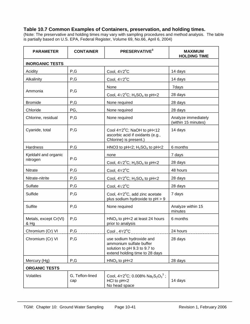
TGM: Chapter 10: Ground Water Sampling Page 10-41 Revision 1, February 2006
Table 10.7 Common Examples of Containers, preservation, and holding times. (Note: The preservative and holding times may vary with sampling procedures and method analysis. The table is partially based on U.S. EPA, Federal Register, Volume 69, No.66, April 6, 2004)
PARAMETER CONTAINER PRESERVATIVE3 MAXIMUM
HOLDING TIME
INORGANIC TESTS
Acidity P,G Cool, 4 2oC 14 days
Alkalinity P,G Cool, 4 2oC 14 days
Ammonia P,G None 7days
Cool, 4 2oC; H2SO4 to pH<2 28 days
Bromide P,G None required 28 days
Chloride PG, None required 28 days
Chlorine, residual P,G None required Analyze immediately (within 15 minutes)
Cyanide, total P,G Cool 4 2oC; NaOH to pH<12 ascorbic acid if oxidants (e.g., Chlorine) is present.)
14 days
Hardness P.G HNO3 to pH<2; H2SO4 to pH<2 6 months
Kjeldahl and organic nitrogen P.G
none 7 days
Cool, 4 2oC; H2SO4 to pH<2 28 days
Nitrate P,G Cool, 4 2oC 48 hours
Nitrate-nitrite P,G Cool, 4 2oC; H2SO4 to pH<2 28 days
Sulfate P,G Cool, 4 2oC 28 days
Sulfide P,G Cool, 4 2oC, add zinc acetate plus sodium hydroxide to pH > 9
7 days
Sulfite P,G None required Analyze within 15 minutes
Metals, except Cr(VI) & Hg
P,G HNO3 to pH<2 at least 24 hours prior to analysis
6 months
Chromium (Cr) VI P,G Cool , 4 2oC 24 hours
Chromium (Cr) VI P,G use sodium hydroxide and ammonium sulfate buffer solution to pH 9.3 to 9.7 to extend holding time to 28 days
28 days
Mercury (Hg) P,G HNO3 to pH<2 28 days
ORGANIC TESTS
Volatiles G, Teflon-lined cap
Cool, 4 2oC; 0.008% Na2S2O33 ;
HCl to pH<2 No head space
14 days

TGM: Chapter 10: Ground Water Sampling Page 10-42 Revision 1, February 2006
PARAMETER CONTAINER PRESERVATIVE3 MAXIMUM
HOLDING TIME
(Acrolein and acrylonitrile
G, Teflon-lined septum
Cool, 4 2oC; 0.008% Na2S2O33,
adjust pH to 4-5 14 days
Dioxins and Furans G, Teflon-lined cap
Cool, 4 2oC 30 days until extraction, 45 days after extraction
Oil and grease G Cool, 4 2oC; H2SO4 or HCl to pH<2
28 days
Phenols G, Teflon-lined cap
Na2S2O3 7 days until extraction, 40 days after extraction
PCBs G, Teflon-lined cap
Cool, 4 2oC 1 year
Pesticides
G, Teflon-lined cap
Cool, 4 2oC; pH 5-9 1 year
RADIOLOGICAL Alpha, beta, and radium
P,G HNO3 to pH<2 6 months
1 Polyethylene (P), Glass (G) 3 For some constituents free Chlorine must be removed by the appropriate addition of Na2S2O3. Shipping When samples are to be shipped to a laboratory, an appropriate container should be used to protect and preserve them. Chests with ice or manufactured blue ice packets are commonly used. However, blue ice packets may not stand up to the rigors of shipping during warm weather. This routinely results in samples being received at the laboratory out of range for temperature. During warm weather, copious amounts of ice are generally recommended. Forms such as a sampling request sheet and/or chain-of-custody containing pertinent information should be included (See page 10-48). Evidence tape also should be placed around the shipping container (and around each container, if desired), to guard against disturbance or tampering. It is important that, if samples are hazardous or potentially hazardous, they meet all federal and state transportation laws. At the state level, contact the Ohio Department of Transportation (ODOT) and the Public Utilities Commission of Ohio (PUCO) for additional information. Not all samples will maintain complete stability, regardless of the preservation technique. Therefore, a limit on when analysis should take place has been set for most parameters (see Table 10.7). These "holding times" specify the maximum allowable time between sample collection and laboratory analysis. Depending on the specific circumstances, if one is exceeded, the sample may need to be discarded and a new sample obtained. Therefore, it is important that the time of sampling and transportation to the lab be documented to ensure that the limits are met. Be aware of analytical holding times and minimize the time between sampling and delivery to the laboratory.
TGM: Chapter 10: Ground Water Sampling Page 10-43 Revision 1, February 2006
DISPOSAL OF PURGED WATER Though it is not the intent of this document to define/determine Ohio EPA's policy on disposal of purged water, the following guidance is provided. In general, purged water should be containerized until the ground water samples are analyzed. If the samples are free from contaminants (e.g., constituent concentrations are not above ambient/natural levels), then it may be acceptable to discharge the purged water onto the ground away from the wellhead but within the limits of the site/facility.15 Purged ground water that exhibits constituent concentrations above ambient/natural quality may need to be managed as wastewater or hazardous waste. If the water has been contaminated by a listed hazardous waste constituent or exhibits, a characteristic of hazardous waste as specified in 3745-51 of the Ohio Administrative Code, it will need to be managed as a hazardous waste. However, if the ground water is treated such that it no longer contains hazardous waste, the ground water would no longer be subject to regulation. Information on this subject can be found at: http://www.epa.gov/correctiveaction/resource/guidance/remwaste/refrnces/12cntdin.pdf If the ground water is known or suspected to contain VOCs, the purged water should be screened with air-monitoring equipment, as well as water-quality field instruments. If these parameters and/or the facility background data suggest that the water is hazardous, it should be contained and disposed of properly as determined on a site-specific basis. DECONTAMINATION PROCEDURES If non-dedicated sampling equipment is used, it should be cleaned between wells to prevent cross-contamination. This includes all non-dedicated equipment that is submerged in a monitoring well or otherwise contacts a ground water sample. The level of decontamination is dependant on the level and type of suspected or known contaminants. A sampling event where high levels of contaminants are known or suspected would require the most stringent decontamination procedure, which may involve the use of solvent rinses. In general, solvent rinses should only be used when high levels of organic contaminants are known or suspected to be present. Care should be taken to avoid the any decontamination product (or breakdown products) from being introduced into the sample. The decontamination area should be upwind of activities that may contribute dust or other contaminants to the solutions used. The process should occur on a layer of polyethylene sheeting to prevent surface soils from coming into contact with the equipment. The effects of cross-contamination can also be minimized by sampling the least contaminated wells first and then progressing to the more contaminated wells. Table 10.8 outlines sequences and procedures that should be used (modified from ASTM D5088-02 and Yeskis and Zavala, 2002). The procedures are based on equipment contact with collected samples. Sample-contacting equipment includes non-dedicated bailers and pumps (i.e., devices used for purging and sampling), sample containers, tubing, downhole field parameter probes, water level probes, non-dedicated filtration equipment, etc. In most
15Under detection monitoring, it may be possible to discharge the purged water without containerizing if historical ground water
records indicate that ground water quality beneath the site is similar to the ambient quality. The Division with authority over the site/facility should be contacted for approval of this disposal method.

TGM: Chapter 10: Ground Water Sampling Page 10-44 Revision 1, February 2006
instances, a distilled water rinse should be sufficient for field parameter measurement probes that are not lowered into wells. Many items are inexpensive and disposable (i.e., gloves, rope, tubing). Items dedicated to a well or disposed of between wells (i.e., gloves, cord, plastic sheet, bailer) would not need to be decontaminated. These items should be properly discarded16 and new materials provided for the next well. Table 10.8 Decontamination procedure for ground water sampling equipment.
Wash with non-phosphate detergent and potable water. Recommend using pressure spray filled with soapy water. Use bristle brush made from inert material to help remove visible dirt.
Rinse with potable water.
If analyzing samples for metals, may* need to rinse with 10% hydrochloric or nitric acid
(note: dilute HNO3 may oxidize stainless steel). This rinse is only effective on non-metallic surfaces.
Rinse liberally with deionized/distilled water.
If analyzing for organics, may* need to rinse with solvent-pesticide grade isopropanol,
acetone, or methanol, alone or if required, in some combination. This solvent rinse should not be an analyte of interest. This rinse is important when a hydrophobic contaminant is present (such as LNAPL or DNAPL, high levels of PCB’s etc.)
Rinse liberally with deionized/distilled water.
Air-dry thoroughly before using.
Wrap with inert material if equipment is not to be used promptly.
*In most cases, solvent rinses will not be needed. Solvent/acid rinses may only be needed when high levels of contaminants are known to be present. DOCUMENTATION Field Sampling Logbook A field logbook or field sampling forms should be completed and maintained for all sampling events. It should document the following for each well sampled17.
Identification of well. Well depth. Static water level depth and measurement technique. Presence of immiscible layers and detection method.
16As discussed in the applicable sampling and analysis plan or equivalent protocol, e.g., a standard operation procedure.
17Items documented on the chain-of-custody do not need to be repeated in the field log.

TGM: Chapter 10: Ground Water Sampling Page 10-45 Revision 1, February 2006
Thickness of immiscible layers, if applicable. Well yield - high or low. Purging device, purge volume and pumping rate. Time well purged. Measured field parameters. Collection method for immiscible layers (if applicable) and identification numbers. Sampling device used. Well sampling sequence. Sample appearance. Types of sample containers and sample identification numbers. Preservative(s) used. Parameters requested for analysis. Field analysis data and method(s). Sample distribution and transporter. Field observations on sampling event. Name of collector(s). Climatic conditions (e.g., air temperature, precipitation, and wind conditions Problems encountered and any deviations made from the established sampling
protocol.
Chain-Of-Custody A chain-of-custody record should be established to provide the documentation necessary to trace sample possession from time of collection to final laboratory analysis. The record (Figure 10.3) should account for each sample and provide the following information: (U.S. EPA, 1992).
Sample identification number. Printed name and signature of collector. Date and time of collection. Sample type (i.e., ground water). Identification of well. Number and types of containers. Parameters requested for analyses. Preservatives used. Carrier used. Printed name and signature of person(s) involved in the chain of possession18.
Date/time samples were relinquished by sampler and received by the laboratory Internal temperature of shipping container upon opening at laboratory, if applicable. Special handling instructions (if any).
18Including all persons relinquishing the samples and all persons receiving the samples, but excluding the U.S. Postal Service, courier services, or commercial shipping companies.
TGM: Chapter 10: Ground Water Sampling Page 10-46 Revision 1, February 2006
Sample Analysis Request Sheet A request sheet may also accompany samples on delivery to the laboratory. However, the chain-of-custody may be used as the sampling analysis request sheet if it contains the following information. Figure 10.4 is an example of a typical sheet.
Sample type (e.g., ground water). Sample identification number. Name of person receiving the sample. Date and time of sample collection. Date of sample receipt. Analyses to be performed. Analysis method requested (if needed). Name of sampler. Internal temperature of shipping container upon opening at the laboratory.
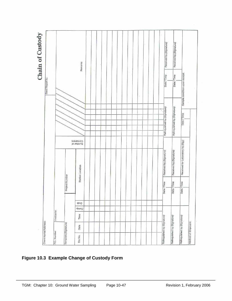
TGM: Chapter 10: Ground Water Sampling Page 10-47 Revision 1, February 2006
Figure 10.3 Example Change of Custody Form

TGM: Chapter 10: Ground Water Sampling Page 10-48 Revision 1, February 2006
Figure 10.4 Example Analysis Request Form
TGM: Chapter 10: Ground Water Sampling Page 10-49 Revision 1, February 2006
FIELD QUALITY ASSURANCE/QUALITY CONTROL (QA/QC) To assure adequate QA/QC in the field, the sampling plan should be followed consistently. To verify if procedures are contaminating ground water samples, a variety of samples and blanks need to be collected and analyzed. The following are typical checks:
Field Duplicates - Field duplicates are samples collected as close to each other in time and space as practical at a specific location. Ultimately, upon analysis, both should yield the same results within an acceptable range. Excessive variation could indicate problems with the sampling procedures or problems with the analysis. If strict protocols are followed, variability as a result of the field procedures should be minimal. At minium, duplicates should be collected at a frequency of one per twenty samples (Yeskis and Zavala, 2002), one per week, and one per sampling event.
Trip Blanks - Trip blanks are generally prepared by the laboratory before entering the
field. Containers are filled with analyte-free, distilled, deionized water and sealed. These blanks are taken to the field and handled along with the collected samples, thereby acting as a control sample to determine potential VOC contamination from the containers themselves. Trip blanks should be included in each cooler containing VOC samples. At, minimum, at least one trip blank should accompany each sampling event. Trip blanks are never opened in the field.
Equipment Blanks - Whenever non-dedicated sampling equipment is used, equipment/field blanks should be collected. An equipment/field blank is obtained by passing analyte-free, distilled, deionized water through a cleaned sampling apparatus (pump, bailer, filtration gear, etc.) and collecting it in a clean container. This blank is used to assess the effectiveness of the decontamination procedures implemented between sampling locations. Ideally, equipment blanks should be collected after sampling the well(s) that historically show(s) highest levels of contamination. They should be collected at a frequency of one blank per 20 samples (Yeskis and Zavala, 2002), one per week, and one per sampling event.
Field Blanks - Field blanks (also known as ambient blanks) are containers containing
de-ionized water, which are opened and remain open during field operations. They are used to assess whether there is a potential for sample contamination from air sources in the surrounding area. Analysis from field blanks cannot be used to adjust sample results. Field blanks are rarely collected as a control measure.
Temperature Blank - A temperature blank may be used to estimate the sample
temperature at the time the sample is received by the laboratory (ASTM, D6517-00). Trip blanks and equipment blanks may not be necessary if it is assumed that any chemical of concern detected is present in the ground water or confirmation sampling and analysis is conducted. All duplicates and blanks should be subjected to the same analysis as the ground water samples. The results are used to determine if proper procedures were followed. Blank
TGM: Chapter 10: Ground Water Sampling Page 10-50 Revision 1, February 2006
contamination can result from improper decontamination of sampling equipment, poor sampling and handling procedures, contaminated rinse water or preservatives, or the interaction between sample and container. The concentration levels of any contaminants found should not be used to correct the ground water data. Blank contamination should trigger a re-evaluation of procedures to determine the source of the problem.
GROUND WATER SAMPLE ANALYSIS SELECTION OF ANALYTICAL METHOD The selection of the method for ground water analysis is determined by the parameters of interest and the purpose of the investigation. Several methods may exist for the same parameter. The selected analytical method should be capable of accurately measuring the constituent of concern in the sample. Some regulatory programs may mandate that the analytical method be U.S. EPA-approved or may suggest a preferred method. Therefore, it is recommended that one check with the regulatory program prior to specifying an analytical method. There are different methods that are approved by U.S. EPA. The following web sites may be helpful in choosing an appropriate method: http://www.epa.gov/epahome/standards.html (U.S. EPA tests methods and guidance), http://www.epa.gov/epaoswer/hazwaste/test/main.htm (U.S. EPA, SW-846 manual), and http://www.epa.gov/SW-846/info.htm (U.S. EPA Web site that provides links to other sites).
The most important analytical requirement generally is the detection limit. For example, claims that no contamination is present in ground water samples are correct only to the quantitative extent that the analysis is capable of detecting the contaminant (Vitale et al., 1991). This level is known as the method detection limit (MDL). The MDL is the minimum concentration of a substance that can be measured and reported with a 99% confidence that the analyte concentration is greater than zero. Useless data may result if the detection limits are not low enough for the purpose of the investigation. For example, the primary objective often is to determine the risk to human health and the environment. In this case, the MDLs should be at or below human health-based criteria and environmental-based criteria. Due to matrix interference and irregularities in instruments, the MDL may not always be obtained. In addition, the actual detection limit will be higher for samples that require dilution or reduced size to avoid saturation of the detector. The actual limit attained during the analysis should be reported with the data. LABORATORY QUALITY ASSURANCE/QUALITY CONTROL (QA/QC) It is not the intent of this document to discuss laboratory QA/QC procedures. Procedures, methods, and levels of quality control are discussed in various U.S. EPA publications (1979a, 1979b, and 1986b). Laboratory QA/QC may include, but may not be limited to, qualifications, performance, matrix effects (e.g., blanks and matrix spikes), documentation, and record reporting. For sites under the CERCLA process, Ohio EPA-DERR (1990) has established set guidelines and specifications for preparing quality assurance project plans.

TGM: Chapter 10: Ground Water Sampling Page 10-51 Revision 1, February 2006
For additional information on QA/QC plans the reader is referred to the Ohio EPA, Division of Hazardous Waste Data Validation Guidance. To obtain reliable results, appropriate laboratory procedures and methods should be followed. An extensive laboratory QA/QC program ensures the production of scientifically sound, defensible results that can be documented and verified. Whether Ohio EPA review is required depends on the regulatory program involved. For example, submittal of a laboratory QA/QC plan is not required for sites undergoing RCRA closure (Ohio EPA, DHWM Program); however, the owner/operator should demonstrate that the laboratory has a plan that contains the elements listed by U.S. EPA (1986b). A laboratory QA/QC plan should be approved for sites remediated under the CERCLA process (Ohio EPA, DERR program). An appropriate level of laboratory QA/QC data should be submitted with sample results to allow verification that the samples were properly handled and analyzed. A particular regulatory program may dictate the amount and type of data. All QA/QC data should be kept and made available upon request. This data may be valuable for explaining outliers and questionable results. However, the laboratory QC results should not be used to alter the sample analytical data. A report on analytical data is incomplete without some verification of laboratory QA/QC.

TGM: Chapter 10: Ground Water Sampling Page 10-52 Revision 1, February 2006
REFERENCES Aller, L., T. W. Bennett, G. Hackett, R. J. Petty, J. H. Lehr, H. Sedoris, D.M. Nielsen, and J. E.
Denne. 1991. Handbook of Suggested Practices for the Design and Installation of Ground Water Monitoring Wells. Environmental Monitoring Systems Laboratory, Office of Research and Development, U.S. Environmental Protection Agency. Las Vegas, Nevada. EPA/600/4-89/034. (In cooperation with National Water Well Association).
American Society for Testing and Materials (ASTM), Method D4448-01. Standard Guide for
Sampling Groundwater Monitoring Wells. American Society for Testing and Material Standards. West Conshohocken, Pennsylvania.
ASTM, Method D4750-87(Reapproved 2001) Standard Test Method For Determining
Subsurface Liquid Levels in a Borehole or Monitoring Well (Observation Well). American Society for Testing and Material Standards. West Conshohocken, Pennsylvania.
ASTM, Method D5088-02. Practice for Decontamination of Field Equipment Used at
Nonradioactive Waste Sites. American Society for Testing and Material Standards. West Conshohocken, Pennsylvania.
ASTM, Method D6634-01. Standard Guide for the Selection of Purging and Sampling Devices
for Ground-Water Monitoring Wells. American Society for Testing and Material Standards. West Conshohocken, Pennsylvania.
ASTM D6517-00. Standard Guide for Field Preservation of Ground-Water Samples. American
Society for Testing and Material Standards. West Conshohocken, Pennsylvania.
ASTM, Method D6699-01. Standard Practice for Sampling Liquids Using Bailers. American Society for Testing and Material Standards. West Conshohocken, Pennsylvania
ASTM Method D6771-02. Standard Practice for Low-Flow Purging and Sampling for Wells
and Devices Used For Ground Water Quality Investigations. American Society for Testing and Material Standards. West Conshohocken, Pennsylvania
Anastas, M. Y. and H. J. Belknap. 1980. Summary of Available Portable VOC Detection
Instruments, PEDCO Environmental. EPA Report No. 340/1-80-010.
Backhus, D.A., J.N. Ryan, D.M. Groher, J.K. MacFarlane, and P.M. Gschwend. 1993. Sampling Colloids and Colloid-Associated Contaminants in Ground Water. Ground Water, Vol. 31, No. 3, pp. 466-479.
Barcelona, M. J., J. P. Gibb, J. A. Helfrich, and E. E. Garske. 1985. Practical Guide for Ground-Water Sampling. Illinois State Water Survey. Champaign, Illinois. Contract Report 374.
TGM: Chapter 10: Ground Water Sampling Page 10-53 Revision 1, February 2006
Barcelona, M.J., J.A. Helfrich, and E.E. Garske. 1988. Verification of Sampling Methods and Selection of Materials for Ground Water Contamination Studies. In A.G. Collins and A.I. Johnson (editors), Ground-Water Contamination: Field Methods. ASTM STP963 ASTM, Philadelphia, PA.
Barcelona, M. J., H. A. Wehrmann, M. R. Schock, M. E. Sievers, and J. R. Karny. 1989.
Sampling Frequency for Ground-Water Quality Monitoring. U.S. EPA Project Summary. EPA/600/S4-89/032.
Barcelona, M.J., H.A. Wehrman, and M.D. Varljen. 1994. Reproducible Well-Purging
Procedures and VOC Stabilization Criteria for Ground-Water Sampling. Ground Water. Vol. 32, No. 1, pp. 12-22.
Brown, G. E., D. A. DuBose, W. R. Phillips and G. E. Harris. 1980. Response Factors of VOC
Analyzers Calibrated with Methane for Selected Organic Chemicals. U.S. EPA, Research Triangle Park, EPA 600/2-81-002.
Brownlow, A.H. 1979. Geochemistry. Prentice-Hall. 498 p.
Dalton, M. G., B. E. Huntsman, and K. Bradbury. 1991. Acquisition and Interpretation of Water-Level Data. In: D. M. Nielsen (editor), Practical Handbook of Ground-Water Monitoring. Lewis Publishers, Inc. Chelsea, Michigan. pp. 367-397.
Deutsch, W.J. 1997. Groundwater Chemistry, Fundamentals and Applications to
Contamination. CRC Press, LLC. 221 p.
DuBose, D. A., G. E. Brown, and G. E. Harris. 1981. Response of Portable VOC Analyzers to Chemical Mixtures. U.S. EPA, Research Triangle Park, EPA 600/2-81-110.
EPRI (Electrical Power Research Institute). 1985. Field Measurement Methods for
Hydrogeologic Investigations: A Critical Review of Literature.EPRI EA-4301. Environmental, Physical and Chemical Program, Energy Analysis Division. Palo Alto, California.
EPRI. 1987. Sampling Guidelines for Ground Water Quality. EA-4952, Research Project 2485-
1. Land and Water Quality Studies Program, Environmental Division. Palo Alto, California.
Garner, S. 1988. Making the most of Field-Measurable Ground Water Quality Parameters. Ground Water Monitoring Review. Vol. 8, No. 3, pp. 60-66.
Gibb, J.A., R.M. Schuller, and R.A. Griffin. 1981. Procedure for the Collection of
Representative Water Quality Data From Monitoring Wells. Illinois State Water Survey and Illinois State Geological Survey Cooperative Ground Water Report 7, 61pp.
Gibbons, R.D. and M.N. Sara. Statistical Comparison of Metals Concentrations in Filtered and
Unfiltered Ground-Water Samples, in Ground Water Sampling, A Workshop Summary: Dallas, Texas. November 30 - December 2, 1993. U.S. EPA Office of Research and Development, EPA/600/R-94/205, pp. 54-58.
TGM: Chapter 10: Ground Water Sampling Page 10-54 Revision 1, February 2006
Gillham, R. W., M. J. L. Robin, J. F. Barker and J. A. Cherry. 1983. Ground Water Monitoring and Sample Bias. Department of Earth Science, University of Waterloo, Ontario. API Publication 4367. Washington, D.C.
Heath, R.C. 1987. Basic Ground-Water Hydrogeology. United States Geological Survey
Water-Supply Paper 2220, 84p.
Hem, J. H. 1992. Study and Interpretation of the Chemical Characteristics of Natural Water (Third Edition). United States Geological Survey Water-Supply Paper 2254. 264 p.
Herzog, B., L. S. F. Chou, J. R. Valkenburg, and R. A. Griffin. 1988. Changes in Volatile
Organic Chemical Concentrations After Purging Slowly Recovering Wells. Ground Water Monitoring Review. Vol. 8, No. 4.
Imbrigiotta, T. E., J. Gibs, T. V. Fusillo, G. R. Kish, and J. J. Hochreiter. 1988. Field Evaluation
of Seven Sampling Devices for Purgeable Organic Compounds in Ground Water. In: A. G. Collins and A. J. Johnson (editors), Ground Water Contamination: Field Methods, ASTM STP 963. American Society for Testing and Material Standards. Philadelphia, Pennsylvania. pp. 258-273.
ITRC, 2004. Technical and Regulatory Guidance for Using Polyethylene Diffusion Bag
Samplers to Monitor Volatile Organic Compounds in Groundwater. Interstate Technology & Regulatory Council. 39 pp.
Karklins, Steven, 1996. Ground Water Sampling Desk Reference. Wisconsin Department of
Natural Resources-Bureau of Drinking Water and Groundwater.
Kasper, R. B. and J. A. Serkowski. 1988. Evaluation of Sampling Equipment for RCRA Monitoring in a Deep Confined Aquifer. Second Outdoor Action Conference, National Water Well Association. Dublin, Ohio. Vol 1, pp. 445-485.
Kearl, P. M., N. E. Korte, and T. A. Cronk. 1992. Suggested Modifications to Ground Water
Sampling Procedures Based on Observations from the Colloidal Borescope. Ground Water Monitoring Review. Vol. 12, No. 2, pp. 155-161.
Kearl, P. M., N. E. Korte, M. Stites, and J. Baker. 1994. Field Comparison of Micropurging vs.
Traditional Ground Water Sampling. Ground Water Monitoring and Remediation. Vol. 14, No. 4, pp. 183-190.
Lee, G. F. and R. A. Jones. 1983. Guidelines for Sampling Ground Water. Journal of the Water
Pollution Control Federation. Vol. 55, No. 1. pp. 92-96.
Martin-Hayden, J.M. 2000. Sample Concentration Response to Laminar Wellbore Flow: Implications to Ground Water Data Variability. Ground Water, Volume 38, Number 1, pp 12-19.
McCarthy, J.F. and J.M. Zachara. 1989. Subsurface Transport of Contaminants.
Environmental Science and Technology, Vol. 5, No. 23, pp. 496-502.
TGM: Chapter 10: Ground Water Sampling Page 10-55 Revision 1, February 2006
Muska, C. F., W. P. Colven, V. D. Jones, J. T. Scogin, B. B. Looney, and V. Price, Jr. 1986. Field Evaluation of Ground Water Sampling Devices for Volatile Organic Compounds. In: Proceedings of the Sixth National Symposium and Exposition of Aquifer Restoration and Ground Water Monitoring. National Water Well Association. Dublin, Ohio. pp. 235-246.
National Council of the Paper Industry for Air and Stream Improvement (NCASI). 1982. A
Guide to Ground Water Sampling. Technical Bulletin No. 362. New York, New York.
NCASI. 1984. A Laboratory Study of Four Methods of Sampling Ground Water for Volatile Organic Compounds. Technical Bulletin No. 441.
Nielsen, D.M. and Nielsen, G.L. 2006. Ground-Water Sampling In: D. M. Nielsen (editor),
Practical Handbook of Environmental Site Characterization and Ground-Water Monitoring. Taylor & Francis Group, CRC Press. Boca Raton. pp. 959-1112.
Nielsen, D.M. and Nielsen, G.L. 2002 Technical Guidance on Low-Flow Purging & Sampling
and Minimum-Purge Sampling. Second Edition. The Nielsen Environmental Field School, Inc. Galena, Ohio.
Nielsen, D. M. and G. L. Yeates. 1985. A Comparison of Sampling Mechanisms Available for
Small-Diameter Ground Water Monitoring Wells. Ground Water Monitoring Review. Vol. 5, No. 2, pp. 83-89.
Nightingale, H.I. and W.C. Bianchi. 1977. Ground-Water Turbidity Resulting From Artificial
Recharge: Ground Water, Vol. 15, No. 2, pp. 146-152.
Ohio EPA. 2004. Tier 1 Data Validation Manual. Division of Hazardous Waste Management. Columbus, Ohio.
Ohio EPA. May 2003. 2002 305(b) Report, Ohio’s Ground Water Quality. Division of Drinking
and Ground Waters. 78 p. Columbus, Ohio.
Ohio EPA, 1990. Guidelines and Specifications for Preparing Quality Assurance Project Plans. Division of Emergency and Remedial Response. Columbus, Ohio.
Oliveros, J. P., D. A. Vroblesky, and M. M. Lorah. 1988. Increasing Purging Efficiency Through
the Use of Inflatable Packers. Proceedings of the Second Outdoor Action Conference on Aquifer Restoration, Ground Water Monitoring and Geophysics. National Water Well Association. Dublin, Ohio. Vol 1, pp. 457-470
Parker, L.V. 1994. The Effects of Ground Water Sampling Devices on Water Quality: A
Literature Review. Ground Water Monitoring and Remediation. Vol. 14, No. 2, pp. 130-141.
Parsons (Parsons Engineering Science, Inc.), 2003. Final Comprehensive Results Report for
the Passive Diffusion Bag Sampler Demonstration Prepared for Air Force Center for Environmental Excellence Technology Division.
TGM: Chapter 10: Ground Water Sampling Page 10-56 Revision 1, February 2006
Paul, D.G., C.D. Palmer and D.S. Cherkauer. 1988. The Effects of Construction, Installation, and Development on the Turbidity of Water in Monitoring Wells in Fine-Grained Glacial Till: Ground Water Monitoring Review. Vol. 8, No. 1, pp. 73-82.
Pennino, J.D. 1988. There’s No Such Thing as a Representative Ground Water Sample
(Editorial). Ground Water Monitoring Review. Vol. 8, No. 3, pp. 4-9.
Pohlmann, K. F. and Hess, J. W. 1988. Generalized Ground Water Sampling Device Matrix. Ground Water Monitoring Review. Vol. 8, No. 4, pp. 82-85.
Powell, R.M., and P.W. Puls. 1993. Passive Sampling Ground Water Monitoring Wells Without
Purging: Multilevel Well Chemistry and Tracer Disappearance. Journal Contaminant Hydrology, Volume 12, pp. 51-77.
Powell, R.M., and P.W. Puls. (no date). Sampling of Ground Water Monitoring Wells, Part 3-
Low Flow and Passive Purging and Sampling. http://www.powellassociates.com
Puls, R.W., D.A. Clark, B. Bledsoe, R.M. Powell, C.J. Paul. 1992. Metals in Ground Water: Sampling Artifacts and Reproducibility. Hazardous Wastes and Hazardous Materials. Vol. 9, No. 2, pp. 149-162.
Puls, R. W. and M. J. Barcelona. 1996. Low-Flow (Minimal Drawdown) Ground Water
Sampling Procedure. Ground Water Issue Paper, U.S. Environmental Protection Agency. EPA/540/S-95/504. 12pp.
Puls, R. W. and M. J. Barcelona. 1989a. Filtration of Ground Water Samples for Metals
Analysis. Hazardous Waste and Hazardous Materials. Vol. 6, No. 4, pp. 385-393.
Puls, R. W. and M. J. Barcelona. 1989b. Ground Water Sampling for Metals Analyses. U.S. EPA Superfund Ground Water Issue, EPA/540/4-89/001.
Puls, R. W., J. H. Eychaner and R. M. Powell. 1990. Colloidal-Facilitated Transport of
Inorganic Contaminants in Ground Water: Part I. Sampling Considerations. U.S. EPA, Environmental Research Brief. EPA/600/M-90/023. Robert S. Kerr Environmental Research Laboratory. Ada, Oklahoma.
Puls, R. W. and R. M. Powell. 1992. Acquisition of Representative Ground Water Quality
Samples for Metals. Ground Water Monitoring Review. Vol. 12, No. 3, pp. 167-176.
Rose, S., and A. Long. 1988. Monitoring Dissolved Oxygen in Ground Water: Some Basic Considerations. Ground Water Monitoring Review. Vol. 8, No. 1, pp. 93-97.
Schrale, G. and J. F. Brandywyk. 1979. An Acoustic Probe For Precise Determination of Deep Water Levels in Boreholes. Ground Water. Vol. 17, No. 1, pp. 110-111.

TGM: Chapter 10: Ground Water Sampling Page 10-57 Revision 1, February 2006
Stolzenburg, T. R. and D. G. Nichols. 1986. Effects of Filtration Method and Sampling on Inorganic Chemistry on Sampled Well Water. Proceedings of Sixth National Symposium and Exposition on Aquifer Restoration and Ground Water Monitoring. National Water Well Association. Dublin, Ohio. pp. 216-234.
Tai, D. Y., K. S. Turner and L. A. Garcia. 1991. The Use of a Standpipe to Evaluate Ground
Water Samplers. Ground Water Monitoring Review. Vol. 11, No. 1, pp. 125-132.
Testa, S.M., and D.L. Winegardner. 1991. Restoration of Petroleum-Contaminated Aquifers. Lewis Publishers, Inc. 269 p.
U.S. EPA. 2004. Guidelines Establishing Test Procedures for the Analysis of Pollutants
Under the Clean Water Act; National Primary Drinking Water Regulations; and National Secondary Drinking Water Regulations; Analysis and Sampling Procedure; Proposed Rule. Federal Register, Tuesday, April 6, 2004. Environmental Protection Agency.
U.S. EPA. 2001. Environmental Investigations Standard Operating Procedures and Quality
Assurance Manual. United States Environmental Protection Agency, Region IV. Athens, Georgia.
U.S. EPA. 2000. Guidance for the Data Quality Objectives Process. United States
Environmental Protection Agency, Washington, D.C. EPA/600/r-96/055
U.S. EPA. 1997. Proceedings of the Symposium on Natural Attenuation of Chlorinated Organics in Ground Water. EPA/540/R-97/504. Office of Research and Development. Washington, D.C.
U.S. EPA 1996a. How to Effectively Recover Free Product at Leaking Underground Storage
Tank Sites. A Guide for State Regulators. United States Environmental Protection Agency. Office of Underground Storage Tanks, OSWER National Risk Management Research Laboratory. http://www.epa.gov/OUST/pubs/fprg.htm
U.S. EPA. 1996b. Test Methods: SW846, Chapter 4-Organic Analysis. Revision 3. United
States Environmental Protection Agency.
U.S. EPA. 1989. Risk Assessment Guidance for Superfund. Volume 1. Human Health Evaluation Manual (Part A). EPA/540/1-89/002. Office of Emergency and Remedial Response. Washington, D.C.
U.S. EPA. 1991. Exposure Point Concentrations in Ground Water. United States
Environmental Protection Agency, Region III. Office of Superfund, Hazardous Waste Management. EPA/903/8-91/002.
U.S. EPA. 1992. RCRA Ground-Water Monitoring Draft Technical Guidance. Office of Solid Waste. Washington, D.C.

TGM: Chapter 10: Ground Water Sampling Page 10-58 Revision 1, February 2006
U.S. EPA. 1986a. RCRA Ground Water Technical Enforcement Guidance Document. Office of Waste Program Enforcement, Office of Solid Waste and Emergency Response. OSWER 9950.1. Washington, D.C.
U.S. EPA. 1986b. Test Methods For Evaluating Solid Waste, SW846. Third Edition. Office of
Solid Waste and Emergency Response. Government Printing Office. Washington, D.C.
U.S. E PA 1982. Handbook for Sampling and Sample Preservation of Water and Wastewater. EPA-600/4-82-029. (Available through National Technical Information Service, PB 83-124503. Springfield, VA).
U.S. EPA 1979a. Methods For Chemical Analysis of Water and Wastes. Environmental
Monitoring and Support Laboratories. EPA/600/4-79/020. Cincinnati, Ohio. (Available through National Technical Information Service, PB84-128677. Springfield, VA.).
U.S. EPA 1979b. Handbook of Analytical Quality Control in Water and Wastewater
Laboratories. Environmental Support Laboratories. EPA 600/4-79/019. Cincinnati, Ohio.
U.S.G.S. No date. Use of Passive Diffusion Samplers for Monitoring Volatile Organic Compounds in Ground Water. USGS Fact Sheet 088-1. URL: http://pubs.water.usgs.gov/fs-088-01
Vitale, R. J., O. Braids, and R. Schuller. 1991. Ground-Water Sample Analysis. In David M.
Nielsen (editor), Practical Handbook for Ground-Water Monitoring. Lewis Publishers, Inc. Chelsea, Michigan. pp. 501-540.
Vroblesky, Don, A. 2001. User’s Guide for Polyethylene-Based Diffusion Bag Samplers to
Obtain Volatile Organic Compound Concentrations in Wells. Part 1: Deployment, Recovery, Data Interpretation, and Quality Control and Assurance. U.S.G.S Water-Resource Investigation Report 01-4060. Part 2: Field Tests, U.S.G.S Water-Resource Investigation Report 01-4061.
Vroblesky, Don and Thomas Hyde. 1997. Diffusion Samplers as an Inexpensive Approach to
Monitoring VOCs in Ground Water. Ground Water Monitoring Review, Vol. 17, No. 3, pp. 177-184.
Wiedemeier, T.H., M.A. Swanson, D.E. Moutoux, J.T. Wilson, D.H. Kampbell, J.E. Hansen, and P. Haas. 1997. Overview of the Technical Protocol for Natural Attenuation of Chlorinated Aliphatic Hydrocarbons in Ground Water Under Development for the U.S. Air Force Center for Environmental Excellence in Proceedings of the Symposium on Natural Attenuation of Chlorinated Organics in Ground Water. EPA/540/R-97/504. Office of Research and Development. Washington, D.C., pp. 37-61.

TGM: Chapter 10: Ground Water Sampling Page 10-59 Revision 1, February 2006
Wilde, F.D., D.B. Radtke, J.Gibs, and R.T. Iwatsubo, eds. 1998. National Field Manual for the
Collection of Water Quality Data. U.S. Geological Survey Techniques of Water-Resources Investigation, Book 9, Handbooks for Water Resources Investigation. Variously paginated.
Wilson, N. 1995. Soil and Ground Water Sampling. Lewis Publishers. Yeskis, Douglas, and Bernard Zavala. 2002. Ground-Water Sampling Guidelines for Superfund and RCRA Project Managers. United States Environmental Protection Agency, Technology Innovative Office, Office of Solid Waste and Emergency Reponse Washington D.C.
TGM: Chapter 10: Ground Water Sampling Page 10-60 Revision 1, February 2006
APPENDIX A
ADDITIONAL INFORMATION FOR SAMPLING WATER SUPPLY WELLS
Water supply wells are often sampled as part of characterizing a potential pollutant source. This information is helpful for characterizing the extent of a plume and to ensure that the public has a safe source of water. The name(s), address, and phone numbers of the resident or water supply owner/operator, should be obtained, so that they can be informed of the results. Many of the same techniques and protocol for sampling monitoring wells also apply to collecting a representative sample from a water supply. This includes: planning and preparation; sample preservation, sample containers, handling and shipping; and documentation. These are discussed in other sections of this document. However, there are additional conditions/procedures that must be considered when selecting the sampling point and the actual sample. These additional considerations are summarized below. Selecting the Sampling Point The following should be considered when choosing the location to collect a water sample:
Prior to sampling, existing information such as well construction, yield and depth should be obtained. The Ohio Department of Natural Resources, Division of Water keeps records of all well logs. Well log records can be searched on-line at http://www.dnr.state.oh.us/water/. If a well log record does not exist, then the local heath department should be contacted to see if they have any records. Also if no log exists, the depth of the well should be measured, if possible, and compared to the ODNR Ground Water Resource maps. These maps can be obtained at the above cited web link.
The intake of the water supply well should be screened/opened to the targeted ground
water zone of interest.
The tap selected for sample collection should be the closest to the water source and prior to any treatment system. Also, if possible, the sampling point should be prior to entering the residence, office, building, or holding tanks etc. It is noted that for some small systems the first tap down stream from the pressure tank and upstream from any water treatment may be the best tap available.
The sampling tap should be protected from exterior contamination associated with
being to close to a sink bottom or to the ground. Contaminated water or soil from the faucet exterior may enter the bottle during the collection procedure since it is difficult to place a bottle under a low tap without grazing the neck interior against the outside faucet surface. If the tap is too close to the ground for direct collection into the appropriate container, it is acceptable to use a smaller (clean) container to transfer the sample to a larger container. The smaller container should be made of glass or stainless steel, or of the same composition of the sample bottles. Also, if samples are

TGM: Chapter 10: Ground Water Sampling Page 10-61 Revision 1, February 2006
to be collected for bacteria, then the tap needs to be disinfected prior to sampling. The laboratory should provide you with their tap disinfection procedures.
Leaking taps that allow water to discharge from around the valve stem handle and
down the outside of the faucet, or taps in which water tends to run up on the outside of the lip, should be avoided as sampling locations.
Disconnect any hoses, filters, or aerators attached to the tap before sampling. These
devices can harbor a bacterial population if they are not routinely cleaned or replaced when worn or cracked. If disconnection from an aerator, or treatment system, is required, permission should be obtained from the well owner.
Taps where the water flow is not constant should be avoided because temporary
fluctuation in line pressure may cause clumps of microbial growth that are lodged in a pipe section or faucet connection to break loose. A smooth flowing water stream at moderate pressure without splashing should be used. The sample should be collected without changing the water flow. It may be appropriate to reduce the flow for the volatile organic compounds aliquot to minimize sample agitation.
When sampling for bacterial content, the sample container should not be rinsed before
use due to possible contamination of the sample container or removal of the thiosulphate dechlorinating agent (if used). When filling any sample container, care should be taken that no splashing drops of water from the ground or sink enter into either the bottle or cap.
Sampling Technique The following procedures should be followed when collecting samples from water supplies:
1. Ideally, the sample should be collected from a tap or spigot located at or near the well head or pump house and before the water supply is introduced into any storage tanks or treatment units. If the sample must be collected at a point in the water line beyond a pressurization or holding tank, a sufficient volume of water should be purged to provide a complete exchange of fresh water into the tank and at the location where the sample is collected. If the sample is collected from a tap or spigot located just before a storage tank, spigots located inside the building or structure should be turned on to prevent any backflow from the storage tank to the sample tap or spigot. It is generally advisable to open several taps during the purge to ensure a rapid and complete exchange of water in the tanks.
2. If the water system is not actively running, purge the system for at least 15 minutes.
Systems that are actively pumped may require less purging (e.g., 3-5 minutes). After purging for several minutes, measure the stabilization parameters (See page 10-27). Continue to monitor these parameters until three consistent readings are obtained.
3. After three consistent readings have been obtained, samples may be collected.
Samples collected from potable water supplies should not be filtered.

TGM: Chapter 10: Ground Water Sampling Page 10-62 Revision 1, February 2006
A detailed operation/procedural process for sampling water supplies can be found in the following references:
Wilde, F.D., Radtke, D.B., Gibs, Jacob, and Iwatsubo, R.T., eds., September 1999, Collection of Water Samples: U.S. Geological Survey Techniques of Water-Resources Investigations, book 9, chap. A4. http://pubs.water.usgs.gov/twri9A4/
U.S. EPA. 2001. Environmental Investigations Standards Operating Procedures and
Quality Assurance Manual. U.S. Environmental Protection Agency. Region 4. Athens, Georgia. http://www.epa.gov/region4/sesd/eisopqam/eisopqam.html

State of Ohio Environmental Protection Agency
Division of Drinking and Ground Waters
Technical Guidance Manual for Ground Water Investigations Chapter 11
Soil Gas Monitoring For Site Characterization
August 2008 Governor : Ted Strickand Director : Chris Korleski
TECHNICAL GUIDANCE MANUAL FOR
GROUND WATER INVESTIGATIONS
CHAPTER 11
Soil Gas Monitoring For Site Characterization
August, 2008 Revision 1
Ohio Environmental Protection Agency Division of Drinking and Ground Waters
P.O. Box 1049 50 W. Town Street, Suite 700 Columbus, Ohio 43216-1049
Phone: 614-644-2752 http://www.epa.state.oh.us/ddagw/

TGM Chapter 11: Soil Gas Monitoring for Site Characterization 11-i Revision 1, August 2008
PREFACE
This document is part of a series of chapters incorporated in Ohio EPA’s Technical Guidance Manual for Hydrogeologic Investigations and Ground Water Monitoring (TGM), which was originally published in 1995. DDAGW now maintains this technical guidance as a series of chapters rather than as an individual manual. The chapters can be obtained at http://www.epa.state.oh.us/ddagw/tgmweb.aspx. The TGM identifies technical considerations for performing hydrogeologic investigations and ground water monitoring at potential or known ground water pollution sources. The purpose is to enhance consistency within the Agency and inform the regulated community of the Agency’s technical recommendations and the basis for them. In Ohio, the authority over pollution sources is shared among various Ohio EPA divisions, including the Emergency and Remedial Response (DERR), Hazardous Waste Management (DHWM), Solid and Infectious Waste (DSIWM), and Surface Water (DSW), as well as other state and local agencies. DDAGW provides technical support to these divisions. Ohio EPA utilizes guidance to aid regulators and the regulated community in meeting laws, rules, regulations and policy. Guidance outlines recommended practices and explains their rationale. The Agency may not require an entity to follow methods recommended by this or any other guidance document. It may, however, require an entity to demonstrate that an alternate method produces data and information that meet the pertinent requirements. The procedures used to meet requirements usually should be tailored to the specific needs and circumstances of the individual site, project, and applicable regulatory program, and should not comprise a rigid step-by-step approach that is utilized in all situations.

TGM Chapter 11: Soil Gas Monitoring for Site Characterization 11-ii Revision 1, August 2008
Major Changes from the February 1995 TGM
The Ohio EPA Technical Guidance Manual for Hydrogeologic Investigations and Ground Water Monitoring (TGM) was finalized in 1995. This guidance document represents an update to Chapter 11 (Supplementary Methods). Listed below are the major changes from the 1995 version. 1. Changed chapter title from Supplementary Methods to Soil Gas Monitoring for Site
Characterization.
2. Removed section on the use of geophysics.
3. Removed section on In-Situ Ground Water Sampler. The information in that section has been revised and moved to Chapter 15: Use of Direct Push Technologies and Soil and Ground Water Sampling (February, 2005).
4. Noted in introduction that the focus of this chapter is for site characterization rather than obtaining data for vapor intrusion risk assessments. Please check with specific divisions for programmatic guidance on vapor intrusion investigations.
5. Added references for default Henry’s Law constants. Also added the equation to convert between Henry’s Law constants presented in atm-m3/mol and dimensionless Henry’s Law constant.
6. Added information on using DPT for active soil gas sampling.
7. Added a note of caution regarding short circuiting when performing active sampling. A
leak test should be performed to evaluate the possibility of short circuiting.
8. Expanded sections on active sampling methods, passive sampling methods, and surface flux chambers to include information from new and updated references.
9. Included references to new documents that have become available since 1995, including:
Updated existing references.
Added reference to the new ITRC document Vapor Intrusion Pathway: a Practical Guideline.
Added reference to a paper by Blayne Hartman on surface flux chamber method
sampling. Added 1997 US EPA reference Expedited Site Assessment Tools for Underground
Storage Tank Sites.
TGM Chapter 11: Soil Gas Monitoring for Site Characterization 11-iii Revision 1, August 2008
TABLE OF CONTENTS
PREFACE ...................................................................................................................... 11- i MAJOR CHANGES FROM THE FEBRUARY 1995 TGM ............................................. 11- ii TABLE OF CONTENTS ................................................................................................ 11-iii FACTORS OF CONCERN IN SURVEY DESIGN ........................................................ 11- 1
CHEMICAL/BIOLOGICAL CHARACTERISTICS OF CONTAMINANTS ................ 11- 2 SITE PHYSICAL FACTORS ................................................................................... 11- 4 SITE METEOROLOGICAL FACTORS ................................................................... 11- 4
SAMPLING AND ANALYSIS TECHNIQUES ............................................................... 11- 5 ACTIVE SAMPLING METHODS ............................................................................ 11- 5
Probe Installation ............................................................................................... 11- 6 Active Sampling Considerations ........................................................................ 11- 6
PASSIVE SAMPLING METHODS .......................................................................... 11- 7 SURFACE FLUX CHAMBERS .............................................................................. 11- 8 HEAD SPACE MEASUREMENTS ......................................................................... 11- 9
Subsurface Structures ....................................................................................... 11- 9 Soil Samples ..................................................................................................... 11- 9
ANALYSIS TECHNIQUES ......................................................................................... 11- 10 INTERPRETATION OF DATA ................................................................................... 11- 10 REFERENCES ........................................................................................................... 11- 12

TGM Chapter 11: Soil Gas Sampling For Site Characterization 11- 1 Revision 1, August 2008
CHAPTER 11
SOIL GAS MONITORING FOR SITE CHARACTERIZATION Soil gas sampling and analysis can be a rapid and cost-effective approach for preliminary delineation of the areal and/or vertical extent of subsurface contamination by volatile organic compounds (VOCs). Information can be obtained that is useful in developing ground water and soil sampling and analysis programs. Gasoline and many other organic liquids contain VOCs that can be emitted as vapors. If released into the subsurface, vapors emitted will occupy the void spaces between the individual grains within the formation. Soil gas surveys involve sampling and analyzing gases that occupy the pore spaces in the vadose zone. Conventional activities such as ground water sampling of monitoring wells and performance of soil borings always will be necessary to confirm and/or monitor subsurface contamination. When an organic liquid is released into the subsurface, it generally migrates downward under the force of gravity until it reaches the water table. Depending on the characteristics of the liquid, it may float on the surface, sink to the bottom of the water-bearing zone, and/or dissolve into the ground water. Also, the contaminant may, in part, become adsorbed to sediments as it migrates through the vadose zone. Soil gas sampling can be used, in appropriate situations, to detect volatile organic vapors derived from all of these potential sources. The technique is most effective for contaminated soils and water table aquifers and is relatively ineffective for contaminated ground water overlain by extensive confining layers. Soil gas surveying can be used to: 1) detect and identify specific VOCs in the subsurface, 2) determine the concentrations of each component in the gas phase, 3) identify sources and extent of multiple spill events, 4) predict the extent of soil and/or ground water contamination, 5) interpret mode of occurrence of contaminants (liquid, dissolved), 6) identify fuel products (diesel vs. gasoline), 7) help guide the placement of borings and monitoring wells and 8) initially monitor the progress of in-situ bioremediation systems. Benefits of soil gas surveys include low cost, rapid sampling, quantitative analysis of VOCs, thorough site coverage, and timely results. While soil gas sampling is widely employed in vapor intrusion investigations, that use is not the focus of this chapter. Please check with specific divisions for programmatic guidance on vapor intrusion investigations.
FACTORS OF CONCERN IN SURVEY DESIGN Site-specific physical factors such as soil characteristics, geologic heterogeneity, depth to water table, and existence of natural or cultural confining zones affect vapor transport and, hence, the usefulness of soil gas surveys. Chemical and physical factors and concentrations of contaminants affect the degree to which compounds partition into the vapor phase. Changes in barometric pressure, temperature, and moisture content can affect soil gas flux and subsequent interpretation of the data. Also, use of proper sampling and analysis protocol and appropriate instruments with detectors sensitive to the contaminant of interest is required to detect volatiles (Crockett and Taddeo, 1987). Failure to understand and consider these factors can result in erroneous conclusions. Table 11.1 summarizes the factors.

TGM Chapter 11: Soil Gas Monitoring for Site Characterization 11-2 Revision 1, August 2008
Table 11.1. Factors affecting concentrations of soil gas vapors.
CHEMICAL/BIOLOGICAL CHARACTERISTICS Volatility of compounds (solubility and vapor pressure) Mobility in subsurface Concentration gradients Persistence in subsurface (half life, biodegradable capacity,
interaction with other chemicals, etc.) HYDROGEOLOGIC CONTROLS
Properties of the soil media: moisture content, total porosity, air porosity, grain size distribution, organic carbon content, redox potential.
Heterogeneity of the subsurface materials Fluctuating water table Perched aquifer ANTHROPOGENIC CONTROLS Paving and buildings Utility conduits Pumping centers
METEOROLOGICAL CONTROLS Barometric pressure Precipitation regime Temperature
CHARACTERISTICS OF CONTAMINANTS Only chemicals that are present in the vapor phase are appropriate for soil gas sampling. This limits application to investigation of the presence of contaminants such as solvent chemicals and petroleum hydrocarbons, which are characterized by high vapor pressure, low molecular weights, and low aqueous solubilities. These compounds can readily partition out of the liquid and/or ground water and into the soil gas phase as the result of their high gas/liquid partitioning coefficients. In general, the greater the amount of contaminant present, the greater the opportunity for volatiles to exist in soil pores; however, the relationship is not necessarily directly proportional. The amount of an organic compound that can be volatilized is limited (under static conditions) by factors controlling the equilibrium between the liquid and gas phase. Additionally, soil gas evolving from light non-aqueous phase liquids (LNAPLs) exhibit higher contaminant concentrations than soil gas coming from a contaminant in the aqueous phase.

TGM Chapter 11: Soil Gas Monitoring for Site Characterization 11-3 Revision 1, August 2008
The vapor pressure of a compound and its Henry’s Law constant together control the extent to which a chemical partitions into the vapor phase. A compound’s vapor pressure is a measure of the pressure that a vapor exerts when it is in equilibrium with its pure liquid or solid form and predicts the likelihood that the compound will enter into the vapor phase. Compounds with vapor pressures greater than 0.5 mm Hg are considered capable of being detected with active soil gas sampling methods (U.S. EPA, 1997). Likewise, the Henry's Law constant of the compound can be used to determine the likelihood it will enter gas phase. Henry's Law constants are a function of the aqueous solubility, vapor pressure, and molecular weight of a compound. Note that care should be taken to determine the units of Henry’s Law constant. Henry’s Law constants may be expressed a number of ways, but the most common for environmental applications are m3-atm/mol or in its dimensionless form. Conversion between dimensionless Henry’s Law constants (H’) and Henry’s Law constants in m3-atm/mol (H) is performed with the following equation:
(1) Compounds having dimensionless Henry’s Law constants greater than 0.1 are considered to be detectable with active soil gas sampling. Compounds with lower Henry’s Law constants may be detected using passive soil gas techniques, though a precise lower limit is unable to be calculated because of local site and detection variations (U.S. EPA, 1997). Table A-5 of the Division of Hazardous Waste Closure Review Guidance (Ohio EPA, 2006) includes both forms of Henry’s Law constants. The Division of Emergency and Remedial Response, Voluntary Action Program, Support Document for Development of Generic Numeric Standards and Risk Assessment (Ohio EPA, 2002) also provides default values. It must be noted that many factors can influence these approximations. For example, compounds characterized by boiling points below 110o C are most mobile in soil gas (Thompson and Marrin, 1987). Vapors from hydrocarbons with boiling points greater than 150o C are usually detected only in the immediate vicinity of the source because of their low diffusion coefficients and tendency to adsorb onto soils. When evaluating for the potential of ground water contamination, soil gas measurements for petroleum releases should be collected as close to the water table as possible (Thompson and Marrin, 1987). Chemicals that are altered by biological action or chemical transformation may be difficult to detect. Petroleum hydrocarbons may undergo biodegradation, particularly in the upper portions of the soil profile where oxygen is present. However, in the immediate vicinity of a strong hydrocarbon source, such as a leaking underground storage tank, vapors are generally detectable at or very near the ground surface. According to Marrin and Kerfoot (1988), halogenated hydrocarbons can biodegrade under anaerobic conditions. Compounds with minimal halogens can biodegrade under both anaerobic and aerobic conditions. Chlorinated hydrocarbons such as tetrachloroethylene (PCE) and trichloroethylene (TCE) can be biologically dehydrated in the subsurface to produce more volatile compounds (e.g., dichoroethene isomers and vinyl chloride).
TGM Chapter 11: Soil Gas Monitoring for Site Characterization 11-4 Revision 1, August 2008
SITE PHYSICAL FACTORS Successful detection of volatiles by soil gas sampling requires transport of VOCs over some distance. The transport is dependent on the chemical/physical properties of the contaminant and hydrogeologic and soil conditions. The predominant transport mechanisms for soil gas are diffusion and convection. Diffusion is the result of thermal motion of molecules subject to a concentration gradient. Convection is the result of a pressure gradient causing mass flow in a gaseous phase. Both processes are independent of topography or hydraulic gradient. The soil gas concentration tends to decrease with increasing distance both horizontally and vertically away from the source. Studies have shown that concentrations drop more rapidly horizontally than vertically (Crockett and Taddeo, 1987). Though vertical transport by diffusion predicts a linear increase in VOC concentration with depth, hydrogeologic/geologic heterogeneities, soil porosity, moisture content, and sorption equilibria within the subsurface can affect VOC vapor gradients. During the upward migration of soil gas, the vapor may encounter a clay or human-made structure that may cause it to diffuse horizontally and result in a plume that is slightly larger than the source. Vapor transport through wet clays is limited compared to transport across dry porous sand (Crockett and Taddeo, 1987). Paved areas can cause near-surface concentrations to be significantly higher because they prevent off-gassing. Also, migration pathways can be directly influenced by anthropogenic structures such as utility conduits, which are typically backfilled with permeable sand and gravel. Shallow conditions present a difficulty with soil gas surveys because the concentration gradient in soil gas can be very steep and slight variations in the ground water elevation can result in large variations in VOC concentrations. If the water table is close to the surface, it is difficult to acquire samples that are reliable and representative. In addition, if samples must be acquired from 2 feet or less, there is an increased likelihood that they will be diluted by air or affected by barometric pressure. However, Tillman et al. (1989b) caution that it is possible to sample at too great a depth. If this occurs, then accumulations of vapors, such as those that may occur above a contaminated perched water table, may be missed. Slight variations in depth of samples collected close to the water table can produce large apparent concentration variations. Less variability in results is apparent with increased distance above the water table. Thus, an understanding of site geology is vitally important. SITE METEOROLOGICAL FACTORS Meteorological changes such as barometric pressure, temperature, and moisture content can affect soil gas flux; therefore, these effects need to be understood in the acquisition and interpretation of data. A high pressure system during sampling creates a lower volatile flux at shallow depths than during a period of low pressure. Freezing and thawing conditions can have an effect on flux. Soil gas can become concentrated beneath the frozen cap. The temperature of soil gas can affect the rate at which volatilization occurs in the subsurface. Studies have shown that VOC concentrations can increase during early afternoon and decrease in late afternoon, roughly correlating with daily temperature changes (Karably and Babcock, 1989). Increased moisture content can increase the rate of movement of volatiles through soils because water tends to displace non-ionic species from the adsorption site. However, according to Tillman et al. (1989a), a period of heavy rainfall often causes a

TGM Chapter 11: Soil Gas Monitoring for Site Characterization 11-5 Revision 1, August 2008
decrease in the gas flux due to the near-surface saturated conditions and the stripping of soluble components out of the soil gas. To eliminate the effects of meteorological changes, soil gas samples should be taken over the shortest period of time possible.
SAMPLING AND ANALYSIS TECHNIQUES Appropriate methods for soil gas sample acquisition and analysis depend on site conditions and survey objectives. Before methods are selected, contaminant properties, site-specific hydrogeologic conditions, human-made interferences, and why and how the data will be utilized should be understood clearly (Crockett and Taddeo, 1987). Accurate detection of VOCs requires use of proper protocol and appropriate instruments with detectors sensitive to the contaminant of interest. The selection of techniques influences the subsequent interpretation of the data. Soil gas sampling techniques fall into several categories: active, passive, surface flux chambers, and head space measurements. The techniques selected should be dependent on the objective of the study. It is imperative that those conducting surveys are experienced with the methods and are familiar with site conditions. ACTIVE SAMPLING METHODS Active sampling methods provide an instantaneous picture of the soil atmosphere at a particular location. Active techniques involve physically withdrawing soil gas through probes or sampling points installed in the soil, usually by pumping. Active methods are necessary for quantitative analysis, and are most useful when the chemicals of concern (COCs) are VOCs. Active soil gas sampling may be used to identify releases, delineate contaminant source areas and VOC plumes, to optimize the placement of soil borings and monitor wells, and to monitor the effectiveness of remedial systems (U.S. EPA, 1997).
Active sampling methods are particularly useful when the following are desirable:
Vertical profiling information Three-dimensional information Real time data Quantitative contaminant data.
However, active soil gas sampling may not be effective for identifying semi-volatile organic compounds (SVOCs) or low volatility compounds. It is not easily conducted in soils with very low permeability or high soil moisture content soils (US EPA, 1997). Probe Installation Soil gas can be sampled by driving a hollow probe into a borehole using a slam bar, direct push technology (DPT), or larger drill rigs, and evacuating a small amount of vapor. Openings in the tube near the leading edge allows for soil gas to enter. The sample can be extracted by inserting a needle through the evacuation line and drawing gas from the stream, or by withdrawing a sample through inert tubing inserted into the probe. Sample tubes can also be buried to create more permanent sample locations. Multilevel samplers may be

TGM Chapter 11: Soil Gas Monitoring for Site Characterization 11-6 Revision 1, August 2008
created by nesting sample tubes within a single borehole. Samples can be analyzed in the field by gas chromatography (GC) or transported for laboratory analysis. Both large-volume and small-volume probes have been used. The internal volume of the probe significantly affects the measurement process and the utility of the resulting data (Devitt et al., 1987). Small probes can be used to attempt to measure "true" soil gas concentrations. The small volume permits the air inside the probe to be purged and a small (e.g., 1 mL) sample to be collected without substantially altering the gas equilibrium. The use of a large probe typically involves sampling several liters of soil gas. This may not permit a representative sample to be collected under most conditions, but allows for the soil gas to be concentrated prior to analysis or for multiple aliquots to be extracted. The large probes are typically used for investigations that seek to determine relative concentrations or that are concerned with whether or not contamination affects a given area. Devitt et al. (1987) cited various researchers and how they applied both small and large probes. Driven probes can be installed through landscaped areas, through concrete or asphalt covers, or inside buildings with relatively little disturbance of the surrounding area. The technique is relatively sensitive and can be used to measure subsurface gas concentrations while avoiding surface interference. Samples also can be obtained below impermeable layers. The technique is well suited for ground water investigations, except in the presence of wet or clayey soils or near surface rock strata. The method is labor- and time-intensive, and sampling ports can clog, making sample extraction difficult. DPT platforms and tools are often used for soil gas sampling. DPT systems may be used to obtain one-time grab samples, or to install soil gas implants for long-term monitoring (McCall et. al, 2006). A number of different systems have been developed for soil gas sampling, and are listed in Chapter 15. Active Sampling Considerations Due to a lack of connected air-filled pores, active soil gas methods generally are not effective at high soil moisture content (above 80- to 90- percent saturation). Sampling procedures can be used to compensate for high soil moisture conditions, but these methods are often time consuming (U.S. EPA, 1997). It is important to use sample techniques that minimize the vacuum applied to the soil to reduce the potential for desorption of contaminants from soil, especially when sampling fine-grained materials (ITRC, 2007). Testing should be conducted to determine the optimal purge volume and rate for the soil conditions. Varying the purge volume and rate until the contaminant concentrations stabilize can determine the optimal volume and rate for sampling. Improper sealing of a sampling probe can allow atmospheric gases to be exchanged with soil gas, commonly known as short circuiting. Rapidly decreasing contaminant levels during sampling, or detection of atmospheric gases, can indicate short circuiting is occurring. Sealing the probe hole, typically done using wet bentonite, can minimize the potential for short circuiting and help ensure that the sample being retrieved is composed of actual soil

TGM Chapter 11: Soil Gas Monitoring for Site Characterization 11-7 Revision 1, August 2008
gas from the sampling depth. A leak test should be conducted using a tracer compound or a “shut-in” test (U.S. EPA, 1997). More information on short circuit testing can be found in ITRC (2007). PASSIVE SAMPLING METHODS Passive soil gas sampling involves use of a sorbent sampler. The device is buried underground and used to collect gas over a given period of time (2 to 6 weeks), after which the devices are removed and analyzed in the laboratory. Devitt et al. (1987) discussed sorbent systems designed by various researchers. Best suited where low concentrations are expected, sorbent samplers provide integrated samples that compensate for fluctuations in soil gas concentration (Devitt et al., 1987). Passive sampling methods are more effective than active sampling when the COCs include SVOCs and low volatility compounds. They are also more effective in low permeability and high moisture soils (U.S. EPA, 1997). The sampling duration can be varied to ensure that a sufficient sample is collected to allow for analytical detection. Since gas-phase diffusivity, which would enable a calculation of concentration from the adsorbed mass in the sampler, is unknown in the vadose zone, contaminant concentration data cannot be determined from this method (ITRC, 2007). Therefore, while passive sampling is useful for determining whether contamination exists, it but does not provide quantitative information. Because the sampling devices are installed just below the ground surface (between 3 inches and 4 feet), installation is quick and a large number of devices can be installed per day. However, the use of passive devices requires a much greater turnaround time for sample acquisition. Some techniques may cause dilution of samples by mixing with the air or cause contamination of the sample from the sampling apparatus (U.S. EPA, 2997). As they are both less expensive and less intrusive than active sampling methods, as well as being easy to deploy, passive sampling methods are particularly useful for obtaining screening level information, particularly at large sites. If vertical data or quick sample turn-around are not required, passive sampling can be a cost-effective sample method. Table 11.2 provides a comparison of active versus passive soil gas sampling applications.
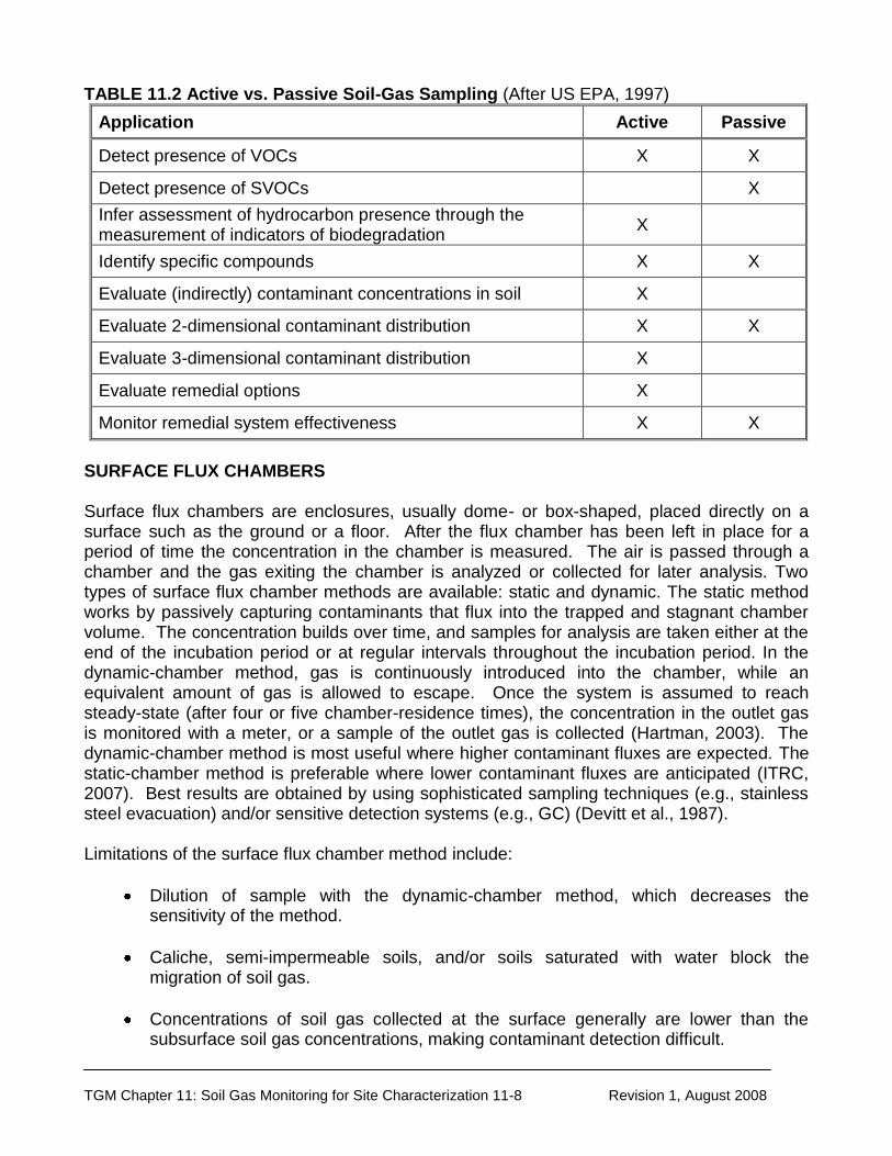
TGM Chapter 11: Soil Gas Monitoring for Site Characterization 11-8 Revision 1, August 2008
TABLE 11.2 Active vs. Passive Soil-Gas Sampling (After US EPA, 1997)
Application Active Passive
Detect presence of VOCs X X
Detect presence of SVOCs X
Infer assessment of hydrocarbon presence through the measurement of indicators of biodegradation
X
Identify specific compounds X X
Evaluate (indirectly) contaminant concentrations in soil X
Evaluate 2-dimensional contaminant distribution X X
Evaluate 3-dimensional contaminant distribution X
Evaluate remedial options X
Monitor remedial system effectiveness X X
SURFACE FLUX CHAMBERS Surface flux chambers are enclosures, usually dome- or box-shaped, placed directly on a surface such as the ground or a floor. After the flux chamber has been left in place for a period of time the concentration in the chamber is measured. The air is passed through a chamber and the gas exiting the chamber is analyzed or collected for later analysis. Two types of surface flux chamber methods are available: static and dynamic. The static method works by passively capturing contaminants that flux into the trapped and stagnant chamber volume. The concentration builds over time, and samples for analysis are taken either at the end of the incubation period or at regular intervals throughout the incubation period. In the dynamic-chamber method, gas is continuously introduced into the chamber, while an equivalent amount of gas is allowed to escape. Once the system is assumed to reach steady-state (after four or five chamber-residence times), the concentration in the outlet gas is monitored with a meter, or a sample of the outlet gas is collected (Hartman, 2003). The dynamic-chamber method is most useful where higher contaminant fluxes are expected. The static-chamber method is preferable where lower contaminant fluxes are anticipated (ITRC, 2007). Best results are obtained by using sophisticated sampling techniques (e.g., stainless steel evacuation) and/or sensitive detection systems (e.g., GC) (Devitt et al., 1987). Limitations of the surface flux chamber method include:
Dilution of sample with the dynamic-chamber method, which decreases the sensitivity of the method.
Caliche, semi-impermeable soils, and/or soils saturated with water block the
migration of soil gas.
Concentrations of soil gas collected at the surface generally are lower than the subsurface soil gas concentrations, making contaminant detection difficult.

TGM Chapter 11: Soil Gas Monitoring for Site Characterization 11-9 Revision 1, August 2008
HEAD SPACE MEASUREMENTS Head space measurements are useful for screening an area during preliminary evaluation. They can be obtained from subsurface structures or from soil samples. Subsurface Structures Head space measurements from subsurface structures involve collecting grab samples or utilizing a portable hydrocarbon analyzer in wells, storm sewers, underground utility lines, or other human-made structures. This technique can be used during the first phase of an investigation. The results obtained can assist in developing protocol for subsequent work. The limitations of this technique include interference from methane in sewer lines and diffusion of volatile hydrocarbon species out of unsealed structures. In addition, negative test results are inconclusive. Soil Samples Head space measurements of a soil sample (e.g., from a hand auger, driven tube, or split spoon) can also be used. Containers should be properly decontaminated and meet the same standards as containers submitted for laboratory analysis. Several approaches can be taken. The container can be half-filled with soil, sealed, and allowed to equilibrate with the ambient temperature. Measurements can be taken from volatilization of the gas into the vacant space using a portable detector (Holbrook, 1987). Other techniques involve placing the sealed container in a hot water bath (70o C) to volatilize the organic compounds (Jermakian and Majka, 1989). Head space measurements from soil samples typically are simple and quick to perform. They can be used to analyze soil gas from discrete or composite samples at incremental depths down to the water table. This technique has been used to collect shallow soil gas to assess deeper sources of vapors. Devitt et al. (1987) recommended this technique when the sampling crew has a modest level of technical expertise or when sophisticated sampling equipment is neither available nor cost-effective. Limitations include:
Primarily suited for measuring adsorbed organics rather than free organics in the interstitial pore spaces.
Loss of volatile hydrocarbons when the sample is removed from the ground or transferred for analysis.
Loss of volatile hydrocarbons due to degradation of organic compounds from the time
delay between sampling and analysis. Soil type, head space volumes, temperature, handling techniques, and storage times need to be held constant to compare relative concentration levels between samples.

TGM Chapter 11: Soil Gas Monitoring for Site Characterization 11-10 Revision 1, August 2008
ANALYSIS TECHNIQUES A wide variety of techniques exist to analyze soil gas. These range from handheld devices that measure total levels of VOCs to laboratory gas chromatographs that measure minute quantities of individual constituents. The selection of a method is dependent on the objective of the survey and the compounds of interest. Handheld analyzers can be used to measure gross levels of VOCs and using such a device is often one of the first steps of an investigation. The technique is quick, simple, and economical and can save substantial amounts of time and money by providing input data for selection of additional sampling strategies (Devitt et al., 1987). However, because of their high sensitivity to ambient changes, the data obtained from a handheld analyzer cannot be used as a mapping tool (Tillman et al., 1989b). Also, negative test results are inconclusive. The use of a gas chromatograph (GC) is more definitive in identifying individual components of soil gas. Samples can either be analyzed in the field using a portable GC unit or taken to a laboratory for analysis by a laboratory-grade unit. The use of portable GCs generates data on the same day the sampling is completed; however, field GC analysis often is slow overall and may not provide the low detection limits that laboratory technology provide. Mobile labs with laboratory-grade GCs provide top quality results and allow field analysis. Selection of an appropriate detector also is critical to a successful survey. The detector should be sensitive to the volatiles to be analyzed and offer appropriate detection limits. A variety of detectors that measure different classes of VOCs can be used with the gas chromatograph. These include a flame ionization detector (FID), a photoionization detector (PID), an electron capture device (ECD) and the Hall electrolytic conductivity detector. A FID can be used when the objective is to detect the presence of petroleum hydrocarbons. An ECD can be used if the objective is to measure the existence of chlorinated hydrocarbons. The Hall detector may be used to detect halogenated compounds, including vinyl chloride, but it is much less sensitive than the ECD to the primary solvents such as trichloroethene (TCE), tetrachloroethane (PCE), and 1,1,1-trochloroethane (TCA) (Ballestrero et al, 2006). A PID can be used to measure some components of both hydrocarbon and chlorinated hydrocarbons. If the objective is to determine the presence of the full range of EPA Volatile Priority Pollutants, then both the GC/FID and the GC/ECD analysis should be conducted.
INTERPRETATION OF DATA
Including soil gasses affected by biodegradation (e.g., oxygen, carbon dioxide, methane, hydrogen sulfide) in a soil gas survey can supply information regarding contaminant source area and plume, as long as background samples are also collected for comparison. Use of these parameters is effective primarily when the contaminants are SVOCs or non-volatile, or if a volatile contaminant is present but has not been directly detected (U.S. EPA, 1997). To obtain maximum benefits from soil gas data, proper interpretation based on experience and knowledge of the underlying principles is essential (Crockett and Taddeo, 1987). One of the most common mistakes is to extend the interpretation beyond the scope of the survey design (Marrin, 1988). For example, a survey designed to locate contaminant source areas

TGM Chapter 11: Soil Gas Monitoring for Site Characterization 11-11 Revision 1, August 2008
probably is not appropriate for delineating contaminant plume characteristics at the same location. Soil gas surveying is effective only for specific types of contaminants and should be interpreted with careful regard to the physical chemistry of the contaminant and the hydrogeologic environment (Marrin and Kerfoot, 1988). Quantitative relationships between VOC concentrations in soil gas and ground water can be difficult to establish due to variability in subsurface conditions across a site (Marrin, 1988). Even under the most homogeneous conditions, correlation coefficients can only be calculated on an order-of-magnitude basis. Heterogeneities in the subsurface (i.e., moisture content, air-filled porosity, grain size distribution, pavement) cause differences between soil gas and ground water plume characteristics; however, the lack of statistical correlation does not mean that soil gas analyses are not indicative of ground water conditions (Marrin, 1988). Using soil gas contours to define the boundary of a contaminant plume in ground water rarely is successful because compounds characterized by low to moderate air/water partitioning coefficients are not present at high enough concentrations in soil gas to be detected and because compounds with high partitioning coefficients have usually diffused in soil gas beyond the ground water plume (Marrin, 1988).

TGM Chapter 11: Soil Gas Monitoring for Site Characterization 11-12 Revision 1, August 2008
REFERENCES
Ballestrero, T., B. Herzog, and G. Thompson. 2006. Monitoring and Sampling the Vadose Zone. In: David M. Nielsen (editor), Practical Handbook of Ground-Water Monitoring. Lewis Publishers, Inc. Chelsea, Michigan. pp. 207-247.
Crockett, E. L. and A. R. Taddeo. 1987. A Technical Evaluation Of Soil Gas Analysis For
Use at a Hazardous Waste Site. Cambridge Analytical Associates, Inc. Boston, Massachusetts.
Devitt, D. A., R. B. Evans, W. A. Jury, and T. A. Starks. 1987. Soil Gas Sensing for
Detection and Mapping of Volatile Organics. National Water Well Association. Dublin, Ohio.
Hartman, B. 2003. How to Collect Reliable Soil-Gas data for Upward Risk Assessments, Part
2: Surface Flux-Chamber Method. In: LUSTline Bulletin 44. New England Interstate Water Pollution Control Commission. Lowell, Massachusetts. Pp. 14-18.
Holbrook, T. 1987. Hydrocarbon Vapor Definition Using Ambient Temperature Headspace
Analysis. In: Proceedings of the National Water Well Association/American Petroleum Institute (NWWA/API) Conference on Petroleum Hydrocarbons and Organic Chemicals in Ground Water. National Water Well Association. Dublin, Ohio. pp. 317-328.
ITRC. 2007. Vapor Intrusion Pathway: A Practical Guideline. Interstate Technology &
Regulatory Council Vapor Intrusion Team. Jermakian, D. A. and C. J. Majka. 1989. Groundwater Monitoring Needs and Requirements.
Part 6: Application for Field Headspace Analysis and Soil Gas Analysis. Hazardous Materials Control. March/April. pp. 34-38.
Karably, L. S. and K. B. Babcock. 1989. Part 5: The Effects of Environmental Variables on
Soil Gas Surveys. Hazardous Materials Control. Jan/Feb. pp. 36-43. Kerfoot, H. B. 1988. Is Soil Gas Analysis an Effective Means of Tracking Contaminant
Plumes in Ground Water? What are the Limitations of Technology Currently Employed? Ground Water Monitoring Review. Vol. 8, No. 2, pp. 54-57.
Kram, M. L. 2006. DNAPL Characterization Methods and Approaches: Performance and Cost
comparisons. In: David M. Nielsen (editor), Practical Handbook of Ground-Water Monitoring. Lewis Publishers, Inc. Chelsea, Michigan. pp.473-516.
Marrin, D. 1988. Soil Gas Sampling and Misinterpretation. Ground Water Monitoring Review.
Vol. 8, No. 2, pp. 51-54. Marrin, D. and H. B. Kerfoot. 1988. Soil Gas Surveying Techniques. Environmental Science
and Technology. Vol. 22, No. 7, pp. 740-745.

TGM Chapter 11: Soil Gas Monitoring for Site Characterization 11-13 Revision 1, August 2008
McCall, W., D. M. Nielsen, S. P. Farrington, and T. M. Christy. 2006. Use of Direct-Push Technologies in Environmental Site Characterization and Ground-Water Monitoring. In: David M. Nielsen (editor), Practical Handbook of Ground-Water Monitoring. Lewis Publishers, Inc. Chelsea, Michigan. pp. 345-471.
Nielsen, D. M., G. L. Nielsen, and L. M. Preslo. 2006. Environmental Site Characterization.
In: David M. Nielsen (editor), Practical Handbook of Ground-Water Monitoring. Lewis Publishers, Inc. Chelsea, Michigan. pp. 35-205.
Tillman, N. and K. Ranlet and T. J Meyer. 1989a. Soil Gas Surveys: Part 1. Pollution
Engineering. Vol. 21, No. 7, pp. 86-89. Tillman, N., K. Ranlet and T.J. Meyer. 1989b. Soil Gas Surveys. Part II/Procedures.
Pollution Engineering. Vol. 21, No. 8, pp. 79-84. Thompson, G., and D. Marrin. 1987. Soil Gas Contaminant Investigations: A Dynamic
Approach. Ground Water Monitoring Review. Vol. 7, No. 3, pp. 88-93. U.S. EPA, (1997). Soil Gas Surveys. In: U.S. EPA, 1997. Expedited Site Assessment Tools
For Underground Storage Tank Sites. Solid Waste and Emergency Response. EPA 510-B 97-001.

TECHNICAL GUIDANCE MANUAL FOR HYDROGEOLOGICINVESTIGATIONS AND GROUND WATER MONITORING
CHAPTER 12GROUND WATER QUALITY DATA ORGANIZATION AND
INTERPRETATION
February 1995

-ii-
TABLE OF CONTENTS
VALIDATION . . . . . . . . . . . . . . . . . . . . . . . . . . . . . . . . . . . . . . . . . . . . . . . . . . . . . . . . . . . . . . . . . . 12-1ORGANIZATION AND INTERPRETATION TOOLS . . . . . . . . . . . . . . . . . . . . . . . . . . . . . . . . . . 12-1
TABULAR . . . . . . . . . . . . . . . . . . . . . . . . . . . . . . . . . . . . . . . . . . . . . . . . . . . . . . . . . . . . . . . . 12-1MAP . . . . . . . . . . . . . . . . . . . . . . . . . . . . . . . . . . . . . . . . . . . . . . . . . . . . . . . . . . . . . . . . . . . . . . 12-2GRAPHICAL . . . . . . . . . . . . . . . . . . . . . . . . . . . . . . . . . . . . . . . . . . . . . . . . . . . . . . . . . . . . . . 12-3
Bar Charts . . . . . . . . . . . . . . . . . . . . . . . . . . . . . . . . . . . . . . . . . . . . . . . . . . . . . . . . . . . . . . 12-3 XY Charts . . . . . . . . . . . . . . . . . . . . . . . . . . . . . . . . . . . . . . . . . . . . . . . . . . . . . . . . . . . . . . 12-3 Box Plots . . . . . . . . . . . . . . . . . . . . . . . . . . . . . . . . . . . . . . . . . . . . . . . . . . . . . . . . . . . . . . . 12-3
Trilinear Diagrams . . . . . . . . . . . . . . . . . . . . . . . . . . . . . . . . . . . . . . . . . . . . . . . . . . . . . . . 12-6Stiff Diagrams . . . . . . . . . . . . . . . . . . . . . . . . . . . . . . . . . . . . . . . . . . . . . . . . . . . . . . . . . . . 12-7
STATISTICS . . . . . . . . . . . . . . . . . . . . . . . . . . . . . . . . . . . . . . . . . . . . . . . . . . . . . . . . . . . . . . . . . . 12-7MODELING . . . . . . . . . . . . . . . . . . . . . . . . . . . . . . . . . . . . . . . . . . . . . . . . . . . . . . . . . . . . . . . . . . . 12-7DATA INTERPRETATION OBJECTIVES . . . . . . . . . . . . . . . . . . . . . . . . . . . . . . . . . . . . . . . . . . 12-7
IDENTIFICATION OF RELEASES TO GROUND WATER . . . . . . . . . . . . . . . . . . . . . . . . . 12-7RATE OF CONTAMINANT MIGRATION . . . . . . . . . . . . . . . . . . . . . . . . . . . . . . . . . . . . . . . . 12-9EXTENT OF CONTAMINANT MIGRATION . . . . . . . . . . . . . . . . . . . . . . . . . . . . . . . . . . . . 12-11SOURCE OF CONTAMINATION . . . . . . . . . . . . . . . . . . . . . . . . . . . . . . . . . . . . . . . . . . . . . 12-11PROGRESS OF REMEDIATION . . . . . . . . . . . . . . . . . . . . . . . . . . . . . . . . . . . . . . . . . . . . . 12-11RISK ASSESSMENT . . . . . . . . . . . . . . . . . . . . . . . . . . . . . . . . . . . . . . . . . . . . . . . . . . . . . . 12-11
REFERENCES . . . . . . . . . . . . . . . . . . . . . . . . . . . . . . . . . . . . . . . . . . . . . . . . . . . . . . . . . . . . . . 12-12
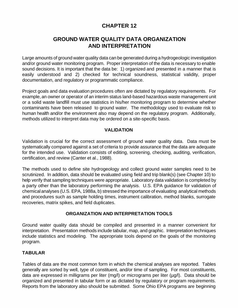
CHAPTER 12
GROUND WATER QUALITY DATA ORGANIZATIONAND INTERPRETATION
Large amounts of ground water quality data can be generated during a hydrogeologic investigationand/or ground water monitoring program. Proper interpretation of the data is necessary to enablesound decisions. It is important that the data be: 1) organized and presented in a manner that iseasily understood and 2) checked for technical soundness, statistical validity, properdocumentation, and regulatory or programmatic compliance.
Project goals and data evaluation procedures often are dictated by regulatory requirements. Forexample, an owner or operator of an interim status land-based hazardous waste management unitor a solid waste landfill must use statistics in his/her monitoring program to determine whethercontaminants have been released to ground water. The methodology used to evaluate risk tohuman health and/or the environment also may depend on the regulatory program. Additionally,methods utilized to interpret data may be ordered on a site-specific basis.
VALIDATION
Validation is crucial for the correct assessment of ground water quality data. Data must besystematically compared against a set of criteria to provide assurance that the data are adequatefor the intended use. Validation consists of editing, screening, checking, auditing, verification,certification, and review (Canter et al., 1988).
The methods used to define site hydrogeology and collect ground water samples need to bescrutinized. In addition, data should be evaluated using field and trip blank(s) (see Chapter 10) tohelp verify that sampling techniques were appropriate. Laboratory data validation is completed bya party other than the laboratory performing the analysis. U.S. EPA guidance for validation ofchemical analyses (U.S. EPA, 1988a, b) stressed the importance of evaluating analytical methodsand procedures such as sample holding times, instrument calibration, method blanks, surrogaterecoveries, matrix spikes, and field duplicates.
ORGANIZATION AND INTERPRETATION TOOLS
Ground water quality data should be compiled and presented in a manner convenient forinterpretation. Presentation methods include tabular, map, and graphic. Interpretation techniquesinclude statistics and modeling. The appropriate tools depend on the goals of the monitoringprogram.
TABULAR
Tables of data are the most common form in which the chemical analyses are reported. Tablesgenerally are sorted by well, type of constituent, and/or time of sampling. For most constituents,data are expressed in milligrams per liter (mg/l) or micrograms per liter (µg/l). Data should beorganized and presented in tabular form or as dictated by regulatory or program requirements.Reports from the laboratory also should be submitted. Some Ohio EPA programs are beginning
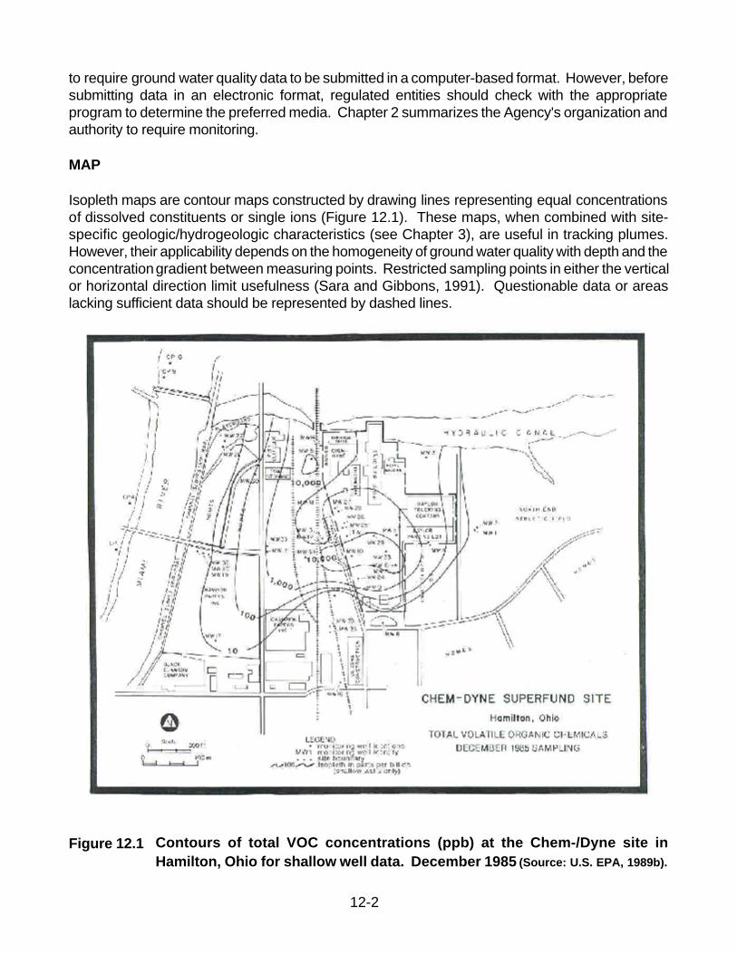
12-2
to require ground water quality data to be submitted in a computer-based format. However, beforesubmitting data in an electronic format, regulated entities should check with the appropriateprogram to determine the preferred media. Chapter 2 summarizes the Agency's organization andauthority to require monitoring.
MAP
Isopleth maps are contour maps constructed by drawing lines representing equal concentrationsof dissolved constituents or single ions (Figure 12.1). These maps, when combined with site-specific geologic/hydrogeologic characteristics (see Chapter 3), are useful in tracking plumes.However, their applicability depends on the homogeneity of ground water quality with depth and theconcentration gradient between measuring points. Restricted sampling points in either the verticalor horizontal direction limit usefulness (Sara and Gibbons, 1991). Questionable data or areaslacking sufficient data should be represented by dashed lines.
Figure 12.1 Contours of total VOC concentrations (ppb) at the Chem-/Dyne site inHamilton, Ohio for shallow well data. December 1985 (Source: U.S. EPA, 1989b).

12-3
GRAPHICAL
Graphical presentation can be helpful in visualizing areal distribution of contaminants, identifyingchanges in water quality with time, and comparing waters of different compositions. Typicalmethods include, but are not limited to, bar charts, XY charts, box plots, trilinear diagrams, and stiffdiagrams.
Bar Charts
Bar charts display a measured value on one axis and a category along the other. Historically, barcharts used in water quality investigations were designed to simultaneously present total soluteconcentrations and proportions assigned to each ionic species for one analysis or group ofanalyses. These charts displayed total concentrations and were based on data reported inmilliequivalents per liter (meq/l) or percent meq/l. Analytes of ground water contamination studiesare present as both ionic and non-ionic species and data are reported in units of mg/l or µg/l. Forsuch studies, bar charts can be constructed to display concentrations of constituents for single ormultiple monitoring wells and/or sampling events. The design and number of the charts shoulddepend on the investigation. Figure 12.2 presents several examples of bar charts that may beuseful.
XY Charts
XY charts differ from bar charts in that both axes show measured parameters. Plots of changes indissolved constituents with time is one example of an XY chart that is extremely useful whenevaluating contaminant releases or remedial progress. Even with a relatively slow rate of flow, long-term monitoring can detect gradual changes. Time-series formats can be used to compareindividual parameters for a single well with time, multiple parameters for a single well with time(Figure 12.3), or illustrate changes with time for multiple wells for a common parameter (Sara andGibbons, 1991). It is important that care be used when evaluating data with different levels of qualityassurance/quality control. Regulated entities are encouraged to supply data in graphical formshowing each parameter for each well plotted against time.
Box Plots
Box plots can be used to compare ground water quality data (generally for the same parameter)between wells. The plots are constructed using the median value and the interquartile range (i.e.,25 and 75 cumulative frequency as measured central tendency and variability) (U.S. EPA, 1992a)(Figure 12.4). They are a quick and convenient way to visualize the spread of data. Complicatedevaluations may dictate use of a series of plots. For example, box plots may be constructed usingdata from wells screened in a particular saturated unit to show horizontal changes in water quality.

12-4
Figure 12.2 Bar Charts. A) Shows concentrations of lead and chromium for one samplingevent. B) Shows concentrations of several consituents at one well overmultiple sampling events.
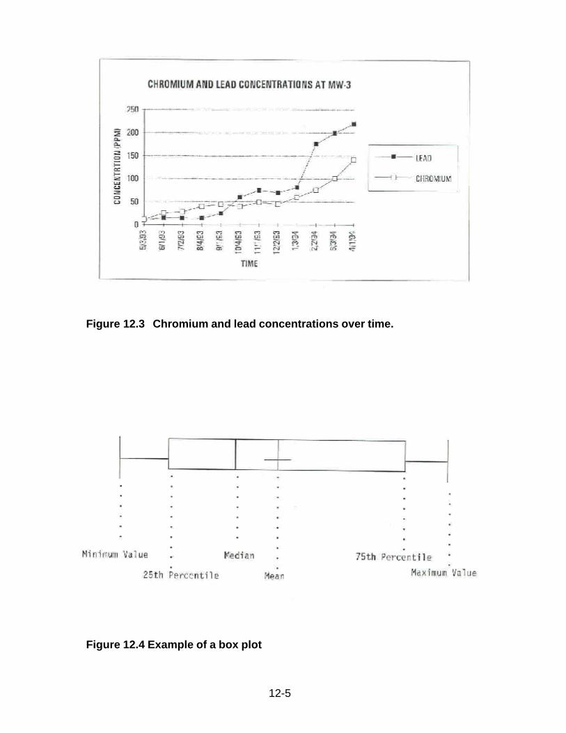
12-5
Figure 12.3 Chromium and lead concentrations over time.
Figure 12.4 Example of a box plot
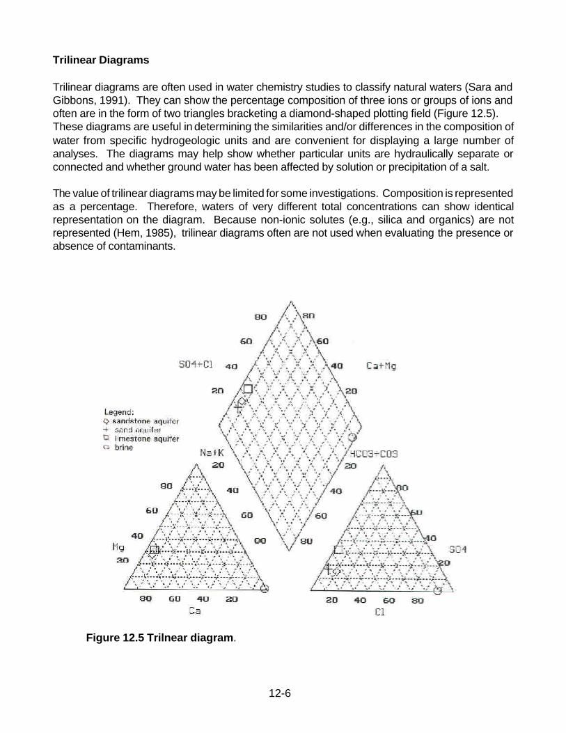
12-6
Trilinear Diagrams
Trilinear diagrams are often used in water chemistry studies to classify natural waters (Sara andGibbons, 1991). They can show the percentage composition of three ions or groups of ions andoften are in the form of two triangles bracketing a diamond-shaped plotting field (Figure 12.5). These diagrams are useful in determining the similarities and/or differences in the composition ofwater from specific hydrogeologic units and are convenient for displaying a large number ofanalyses. The diagrams may help show whether particular units are hydraulically separate orconnected and whether ground water has been affected by solution or precipitation of a salt.
The value of trilinear diagrams may be limited for some investigations. Composition is representedas a percentage. Therefore, waters of very different total concentrations can show identicalrepresentation on the diagram. Because non-ionic solutes (e.g., silica and organics) are notrepresented (Hem, 1985), trilinear diagrams often are not used when evaluating the presence orabsence of contaminants.
Figure 12.5 Trilnear diagram.
12-7
Stiff Diagrams
Stiff diagrams are another graphical representation of the general chemistry of water. A polygonalshape is created from four parallel horizontal axes extending on either side of a vertical axis.Cations are plotted on the left of the vertical axis and anions are plotted on the right (Fetter, 1994). The diagrams can be relatively distinctive for showing water composition differences or similarities.The width of the pattern is an approximation of total ionic strength (Hem, 1985). One feature is thetendency of a pattern to maintain its characteristic shape as the sample becomes diluted. It maybe possible to trace the same types of ground water contamination from a source by studying thepatterns. In the case presented in Figure 12.6, seepage of salt water from a brine disposal pitwas suspected. Samples analyzed from the pit and the wells demonstrated the same pattern,showing evidence of contamination (Stiff, 1951).
STATISTICS
Ground water quality data also can be evaluated by statistical analysis. This tool can be used tocompare upgradient versus downgradient or changes with time. Various regulatory programs mayrequire use of statistics. The reader is referred to Statistical Analysis of Ground Water MonitoringData at RCRA Facilities (U.S. EPA, 1989a), the addendum to that document (U.S. EPA, 1992b),and Chapter 13 for appropriate methodologies.
MODELING
Ground water modeling is a tool that can assist in the determination of extent and rate ofcontaminant migration. Models can be used throughout the investigation and remedial processes.Information on modeling can be found in Chapter 14.
DATA INTERPRETATION OBJECTIVES
The mechanism to interpret ground water quality data can vary depending on project objectives andregulatory or program requirements. Data often are evaluated to: 1) determine if a site/facility hasimpacted ground water (detection monitoring), 2) determine the rate, extent, and concentration ofcontamination (assessment monitoring), 3) determine the source of contamination, 4) gauge theeffectiveness of remedial activities, and/or 5) monitor for potential health or environmental effects.Data must always be evaluated in conjunction with site hydrogeology, contaminant characteristics,and past and present land use.
IDENTIFICATION OF RELEASES TO GROUND WATER
Methods to identify whether contaminants have been released to ground water include professionaljudgment and statistical analysis.
12-8
Figure 12.6 Stiff pattern demonstrating seepage of a salt from a brine disposal pit.
.

1 See Chapter 5 for additional explanation on how these parameters influence ground water flow paths.
12-9
Professional judgment involves the use of education and experience. In some cases, a simplevisual inspection of downgradient versus upgradient/background data can show obvious differencesin chemical quality. The tabular and graphical presentations discussed earlier in this chapter canbe used for this evaluation.
When evaluating potential ground water contamination, water quality data often are compared toprimary and secondary drinking water standards. As important as it is to protect public health byidentifying an exceedance, formulating a conclusion that ground water has been contaminatedbased solely on the exceedance is not appropriate. Certain inorganic constituents, such as iron andsulfate, can occur naturally in Ohio's ground water at levels above standards; therefore, exceedancefor these constituents may not imply contamination. Conversely, values lower than a standard donot necessarily imply that contamination has not occurred. In general, the mere presence oforganics, which usually are not naturally occurring, indicates contamination. Data for wellsdowngradient from a pollution source should be compared to data from an upgradient/backgroundwell that has not been affected by the source. If an upgradient/background well does not exist, thenthe results can initially be compared to known local or regional background values. However,utilization of regional values for evaluating potential contamination should be a part of initialinvestigations only. Further evaluation should be based on site-specific background sampling. Inany ground water contamination investigation, it is essential to obtain background concentrationsfor chemical constituents of concern, particularly those that may be common to both the local groundwater quality and the potential or known contaminant source.
Whether a release has occurred also can be evaluated by statistical analysis if adequate data areavailable. The U.S. EPA (1989a, 1992b) documents and Chapter 13 should be used to determineappropriate methods and application. While statistics are useful to determine if a release occurred,professional judgment still needs to be exercised to ensure that the results represent actualconditions. For example, the results may show either a "false positive" or "false negative" due tonaturally occurring variations such as geologic heterogeneity and/or seasonal variability.Determining whether a release has occurred or whether the analysis has triggered a "false positive"generally requires additional investigation.
RATE OF CONTAMINANT MIGRATION
A simple and straight forward method does not exist for determining the rate of contaminantmigration. In general, the rate can be estimated by a form of Darcy's Law (see Chapter 3) if it isassumed that the dissolved solute travels at the average linear ground water velocity. The rate ofadvancement of a dissolved contaminant can be substantially different, however. Mobility of acontaminant can be altered due to adsorption/desorption, precipitation, oxidation, andbiodegradation. Mobility of a solute can be affected by the ratio of the size of the molecule to thepore size. The calculated velocity also would not account for a contaminant moving faster than theaverage linear velocity due to hydrodynamic dispersion. Dispersion affects all solutes, whereas1
adsorption, chemical reactions, and biodegradation affect specific constituents at different rates.Therefore, a contaminant source that contains a number of different solutes can result in severalplumes moving at different rates.

12-10
MCMt
' [ MMx
(DxMCMx
) %MMy
(DyMCMy
) %MMz
(DzMCMz
)] Dispersion
&[ MMx
(vxC) %MMy
(vyC) %MMz
(vzC)] Advection
±F(c) Reaction
The equation governing the movement of dissolved species can be developed by utilizing theconservation of mass approach. The equation in statement form, as described by Canter et al.(1988), is:
Net rate ofchange of
mass withinan elemental
cell
=flux of solute
out of theelemental
cell
-flux of solute
into theelemental
cell
-+
loss or gainof solute
mass dueto reactions
The mass of solute transported in and out of the cell is controlled by advection and dispersion. Lossor gain of solutes within the cell may be caused by chemical, biological, or adsorption/ desorptionreactions. A generalized three-dimensional solute transport equation considering dispersion,advection, and reactions in a homogeneous environment takes the form as (modified from Freeze& Cherry, 1979):
Where: C = the concentration of the polluting substance;Dx, Dy, Dz = the coefficients of hydrodynamic dispersion in the x, y, z directions;vx, vy, vz = velocity vector components in the x, y, and z directions; andF(c) = chemical reaction function.
Attempts to quantify contaminant transport generally rely on solving conservation of mass equations.There are essentially two kinds of models available for solving mass transport equations, analyticaland semi-analytical, and numerical. Analytical models are developed by considering idealconditions or using assumptions to simplify the governing equation. These assumptions may notallow a model to reflect conditions accurately. Additionally, even some of the simplest analyticalmodels tend to involve complex mathematics. Numerical modeling techniques incorporateanalytical equations that are so complex they necessitate use of computers capable of multipleiterations to converge on a solution (Canter et al., 1988). The numerical approach depends ontedious sensitivity analyses to develop information on the nature of the parameter interaction.Analytical models are used to verify the accuracy of numerical solutions where appropriate.Additional information on numerical, computer-oriented models can be found in Chapter 14.
EXTENT OF CONTAMINANT MIGRATION
The areal or vertical extent of contaminant plumes may range within wide extremes depending onlocal geologic/hydrogeologic conditions. Determination of extent generally involves samplingmonitoring wells at increasing distances and depths from the source. Data for wells downgradient
12-11
of the site/facility are compared to background data by visual inspection and/or statistical analysis.All downgradient locations at which significant differences are noted are considered to be withinthe contaminated area. The use of isopleth maps and time-series formats assist in thedetermination of extent. Modeling (Chapter 14) can be used to help estimate rate and extent anddetermine optimum locations for monitoring wells.
SOURCE OF CONTAMINATION
Ground water quality data often are evaluated to determine the source of contamination. In general,isopleth and ground water contour maps are utilized in conjunction with knowledge of area-specificgeologic/hydrogeologic characteristics, contaminant properties, and past and present land use topinpoint the source.
PROGRESS OF REMEDIATION
When gauging the effectiveness/progress of remedial action, changes in water quality can best beillustrated by time-series presentations and a series of isopleth maps prepared throughout theproceedings. The data should be compared to background or standards developed by riskassessment.
RISK ASSESSMENT
Clean-up goals often are established by means of a risk assessment. Both human health andenvironmental assessments can be conducted. The appropriate methodology depends on theregulatory program involved. Therefore, prior to conducting a risk assessment, the appropriateOhio EPA Division should be consulted.

12-12
REFERENCES
Canter, L. W., R. C. Knox and D. M. Fairchild. 1988. Ground Water Quality Protection. LewisPublishers, Inc. Chelsea, Michigan.
Davis, S.N. and R. J. M. DeWiest. Hydrogeology. John Wiley & Son. New York, New York.
Fetter, C .W. 1994. Applied Hydrogeology. Third Edition. Macmillan College Publishing Company.New York, New York.
Freeze, R. A. and J. A. Cherry. 1979. Groundwater. Prentice-Hall. Inc. Englewood Cliffs, New Jersey.
Hem, J.D. 1985. Study and Interpretation of Chemical Characteristics of Natural Water. Third Edition.Geological Survey Water-Supply Paper 2254. United States Government Printing Office,Washington, D.C.
Sara, M. N. 1994. Standard Handbook for Solid and Hazardous Waste Facilities. Lewis Publishers,Inc., Ann Arbor, Michigan.
Sara, M. N. and R. Gibbons. 1991. Organization and Analysis of Water Quality Data. In: D.M.Nielsen(editor), Practical Handbook of Ground Water Quality. Lewis Publishers, Inc. Chelsea, Michigan.pp. 541-588.
Stiff, H.A., Jr. 1951. The Interpretation of Chemical Water Analysis by Means of Patterns. Journal ofPetroleum Technology. Vol. 3, No. 10, pp 15-17.
U.S. EPA. 1986. RCRA Ground Water Technical Enforcement Guidance Document. Office of WasteProgram Enforcement, Office of Solid Waste and Emergency Response. OSWER 9950.1.Washington, D.C.
U.S. EPA. 1988a. Laboratory Data Validation Functional Guidelines for Evaluating OrganicsAnalyses. Hazardous Site Evaluation Division, Sample Management Office. Washington, D.C.
U.S. EPA. 1988b. Laboratory Data Validation Functional Guidelines for Evaluating InorganicsAnalyses. Hazardous Site Evaluation Division, Sample Management Office. Washington, D.C.
U.S. EPA. 1989a. Guidance Document on the Statistical Analysis of Ground-Water Monitoring Data
at RCRA Facilities--Interim Final Guidance. Office of Solid Waste, Waste Management Division.Washington, D.C.
U.S. EPA. 1989b. Transportation and Fate of Contaminants in the Subsurface. EPA/625/4-89/019.Center for Environmental Research Information. Cincinnati, Ohio.
U.S. EPA. 1992a. A Ground Water Information Tracking System with Statistical Analysis Capacity.United States Protection Agency, Region VII, Kansas City, Kansas.
U.S. EPA. 1992b. Statistical Analysis of Ground Water Monitoring Data at RCRA Facilities.Addendum to Interim Final Guidance. Office of Solid Waste, Waste Management Division.Washington, D.C.
TECHNICAL GUIDANCE MANUAL FOR HYDROGEOLOGICINVESTIGATIONS AND GROUND WATER MONITORING
CHAPTER 13STATISTICS FOR GROUND WATER QUALITY COMPARISON
February 1995

-ii-
TABLE OF CONTENTS
BASIC STATISTICAL ASSUMPTIONS . . . . . . . . . . . . . . . . . . . . . . . . . . . . . . . . . . . . . . . . 13-1INDEPENDENT SAMPLES . . . . . . . . . . . . . . . . . . . . . . . . . . . . . . . . . . . . . . . . . . . . . . 13-2DETERMINATION OF BACKGROUND DATA SET . . . . . . . . . . . . . . . . . . . . . . . . . . 13-3SAMPLING FREQUENCY . . . . . . . . . . . . . . . . . . . . . . . . . . . . . . . . . . . . . . . . . . . . . . . 13-3CORRECTIONS FOR SEASONALITY . . . . . . . . . . . . . . . . . . . . . . . . . . . . . . . . . . . . . 13-3
STATISTICAL ASSUMPTIONS THAT VARY WITH METHODS . . . . . . . . . . . . . . . . . . . 13-3MINIMUM SAMPLE SIZE . . . . . . . . . . . . . . . . . . . . . . . . . . . . . . . . . . . . . . . . . . . . . . . . 13-4DETERMINATION OF DISTRIBUTION . . . . . . . . . . . . . . . . . . . . . . . . . . . . . . . . . . . . . 13-5TRANSFORMATION OF DATA TO ACHIEVE NORMAL DISTRIBUTION . . . . . . . . 13-6NORMALITY TESTS . . . . . . . . . . . . . . . . . . . . . . . . . . . . . . . . . . . . . . . . . . . . . . . . . . . . 13-6HOMOGENEITY OF VARIANCE . . . . . . . . . . . . . . . . . . . . . . . . . . . . . . . . . . . . . . . . . . 13-7TREATMENT OF VALUES BELOW THE DETECTION LIMIT (NON-DETECTS . . 13-7ERRORS . . . . . . . . . . . . . . . . . . . . . . . . . . . . . . . . . . . . . . . . . . . . . . . . . . . . . . . . . . . . . . 13-8
Comparisonwise Error . . . . . . . . . . . . . . . . . . . . . . . . . . . . . . . . . . . . . . . . . . . . . . . 13-8Experimentwise Error . . . . . . . . . . . . . . . . . . . . . . . . . . . . . . . . . . . . . . . . . . . . . . . . 13-8
METHODS . . . . . . . . . . . . . . . . . . . . . . . . . . . . . . . . . . . . . . . . . . . . . . . . . . . . . . . . . . . . . . . 13-9ANOVA . . . . . . . . . . . . . . . . . . . . . . . . . . . . . . . . . . . . . . . . . . . . . . . . . . . . . . . . . . . . . 13-10TWO-SAMPLE TESTS . . . . . . . . . . . . . . . . . . . . . . . . . . . . . . . . . . . . . . . . . . . . . . . . 13-10INTERVALS . . . . . . . . . . . . . . . . . . . . . . . . . . . . . . . . . . . . . . . . . . . . . . . . . . . . . . . . . 13-10
Tolerance Intervals . . . . . . . . . . . . . . . . . . . . . . . . . . . . . . . . . . . . . . . . . . . . . . . . . 13-11Prediction Intervals . . . . . . . . . . . . . . . . . . . . . . . . . . . . . . . . . . . . . . . . . . . . . . . . . 13-11Confidence Intervals . . . . . . . . . . . . . . . . . . . . . . . . . . . . . . . . . . . . . . . . . . . . . . . . 13-12
CONTROL CHART METHOD . . . . . . . . . . . . . . . . . . . . . . . . . . . . . . . . . . . . . . . . . . . . . 13-12STATISTICAL DATA SUBMITTALS . . . . . . . . . . . . . . . . . . . . . . . . . . . . . . . . . . . . . . . . 13-12REFERENCES . . . . . . . . . . . . . . . . . . . . . . . . . . . . . . . . . . . . . . . . . . . . . . . . . . . . . . . . . 13-14
CHAPTER 13
STATISTICS FOR GROUND WATER QUALITY COMPARISONS
The statistical evaluation of data resulting from the chemical analysis of ground water is requiredby Ohio's regulations for Part B permitted hazardous waste land disposal facilities [OAC 3745-54-97(G)], Part A permitted hazardous waste land disposal facilities [OAC 3745-65-93], and permittedmunicipal solid waste [OAC 3745-27-10(C)(6)], residual waste [OAC 3745-30-08(C)(5)], andindustrial waste landfills [OAC 3745-29-10(C)(6)]. Additionally, statistics can be employed forwastewater facilities (including non-toxic flyash, bottom ash, foundry sand and coal storage piles)and in corrective actions at regulated and unregulated hazardous waste sites. This chapter isintended to address only those statistical evaluations performed for Part B permitted hazardouswaste land disposal facilities, permitted municipal solid, residual, and industrial waste landfills, andwastewater facilities. This chapter pertains to Part A permitted hazardous waste land disposalfacilities only if the owner/operator has entered into an agreement with the Director of Ohio EPA toutilize methods identified in OAC 3745-54-97 in place of those specified in OAC 3745-65-93.Regarding the methods mandated by OAC 3745-65-93 (i.e., the Student's T-test and the AverageReplicate Test), the reader is referred to the U.S. EPA's Technical Enforcement GuidanceDocument (U.S. EPA, 1986).
Statistical analyses are used to compare the chemical ground water quality of a monitored zonedowngradient of the waste management unit with either: 1) a standard set in a permit, 2) thechemical ground water quality from a background (or upgradient) well screened in the samemonitored zone and unaffected by facility operations, or 3) historic concentrations from the samewell. These comparisons provide reliable determinations as to whether a waste management unithas influenced the quality of the ground water. Statistics can also be used to define the extent ofground water contamination. If no statistically significant difference is observed between adowngradient well and background, the well is statistically considered beyond the plume ofcontamination. U.S. EPA has issued the Guidance Document on the Statistical Analysis of Ground WaterMonitoring Data at RCRA Facilities, (U.S. EPA, 1989) and an addendum to the same document(U.S. EPA, 1992). The Ohio EPA recommends the methods outlined in the U.S. EPA guidance.Additionally, U.S. EPA has developed a data management tool designed to facilitate the storage,analysis and reporting of data collected through ground water monitoring programs. The statisticalportion of the program incorporates the most frequently used statistical methods for ground watermonitoring. This tool is called the Ground Water Information Tracking System with StatisticalAnalysis Capability (GRITS/STAT or GRITS).
This chapter supplements and clarifies the U.S. EPA's guidance with regard to the number ofdifferent statistical methods required per facility, independent samples, determination of abackground data set, initial year sampling frequency, and corrections for seasonal fluctuations. Inaddition, fixed and variable requirements or assumptions of the most frequently used statisticalmethods are discussed. These assumptions include minimum sample size, distribution, variance,treatment of non-detects, and comparison and experimentwise errors. Finally, recommendationsfor submittals of statistical information are outlined. It is recommended that the U.S. EPA guidancedocuments be reviewed before reading this chapter.

13-2
BASIC STATISTICAL ASSUMPTIONS
Whether starting from scratch with a new database or building on an established database, the firststeps in determining whether a statistically significant difference has occurred should be the same.Before choosing the statistical method, an evaluation must be made as to whether the availablesite-specific data meet a few basic assumptions necessary for a particular test to perform with thegreatest accuracy and power, power being the probability that the test will correctly identifycontamination when it is present. Assumptions basic to all methods include independence ofsamples, determination of the background data set, sampling frequency, and corrections forseasonality.
INDEPENDENT SAMPLES
Statistical analysis is based on the assumption that all data points are generatedindependently of each other. For ground water samples to be independent of each other,enough time must pass between sampling events to ensure that the previously sampled groundwater has left the vicinity of the monitoring well and that "new" ground water is being sampled. Atthe same time, the sampling interval must be short enough to provide "immediate" detection ofcontamination.
Ohio Hazardous Waste Regulations, OAC Rule 3745-54-97(G)(1), 98(D) and 99(F) and (G), requirethe collection of independent samples for permitted facilities. Wastewater policy and solid wasteregulations do not state specifically that independent samples must be collected, but solid wasteregulations do state that the sample number must be appropriate for the statistical method chosen(OAC Rule 3745-27-10(C)(9)). To perform a valid statistical test, including the collection ofindependent samples, the time interval between sampling events should be based on the averagelinear velocity of ground water for the zone being sampled. The sampling interval is determinedafter evaluating the monitored zone's effective porosity, horizontal hydraulic conductivity, hydraulicgradient, and the fate and transport characteristics of potential contaminants. U.S. EPA (1989)outlined the method used to determine the sampling interval necessary to obtain an independentsample.
For wells recovering reasonably quickly, it may be possible to collect multiple independent samplesin one scheduled event by purging a well thoroughly, collecting the first independent sample, thenrepurging the well and collecting the second independent sample, etc., until all necessary sampleshave been collected. If a regulated entity proposes this option, it must supply data indicating therecharge rate of the well. However, to develop a representative background ground water qualitydatabase, temporal and seasonal water level (and parameter) variations must be accounted for.In other words, just because there is adequate recharge does not mean that the completebackground data set may be collected at one sampling event.
Generally, replicate samples are unacceptable for statistical analysis because the information theyprovide indicate only the accuracy of the laboratory, not the ground water quality. When more thanone sample is collected for the same parameter from the same bailer or same aliquot of groundwater, the samples are considered replicate samples. Replicates are not recommended as theyoffer less variability than independent samples. If, however, replicates have been obtained as part

13-3
of the original background data for hazardous waste Part A Interim Status ground water monitoring,and the Ohio EPA approves the use of this data as background for Part B permitted statusstatistical analyses, the replicate values should first be averaged and the means used in thestatistical analyses.
DETERMINATION OF BACKGROUND DATA SET
For all statistical methods employing the use of pooled background data, the backgrounddata set should be such that it reflects naturally occurring changes in hydrogeology. Amoving background data set is recommended using data from only the eight most recent samplingevents. This will help minimize temporal variability (Sara, 1991). During the initial year ofmonitoring, only the background or upgradient well(s) should be used as background whencomparing up to downgradient values. In subsequent years, the background levels, whether usingup to downgradient or intra-well comparisons, should be modified during each monitoring event sothat the eight most recent values are used. When intra-well comparisons are being performed (e.g.,control chart) the background database must be from an uncontaminated well.
SAMPLING FREQUENCY
Minimum sampling frequency shall be consistent with the appropriate statistical methodchosen. The Ohio hazardous waste rules require at least semi-annual sampling for detectionmonitoring (OAC Rule 3745-54-98(D)), while solid waste rules (OAC Rule 3745-27-10(D)(5))require at least semi-annual monitoring for the initial year. However, to determine initialbackground values, sampling must be appropriate for the statistical method chosen (OAC Rule3745-54-97(G)). The hazardous or solid waste permit should outline the sampling frequencynecessary to achieve the minimum sample size, which may oblige the permittee to sample morethan what appears to be regulatorily required.
CORRECTIONS FOR SEASONALITY
Only when strong empirical evidence is present to indicate that seasonality exists shouldcorrections for seasonality be made. If seasonality is present in a data set, Ohio hazardous andsolid waste regulations require procedures be used to control or correct for it. The followingmethods are available: 1) Two-way ANOVA, which attributes variations to seasonal as well asspatial differences, 2) U.S. EPA (1989) provided a simple method for calculating the monthly orquarterly effects attributable to seasonal variations, and 3) Seasonal Kendal Test (Gibbons, 1994).Tolerance intervals tend to be self-correcting for seasonality since seasonal effects show up in bothupgradient and downgradient wells.
STATISTICAL ASSUMPTIONS THAT VARY WITH METHODS
Once the basic assumptions have been met or the data set has been transformed to meet the basicassumptions, a statistical method may be chosen. The next step in making the choice is todetermine the best fit between the site-specific data available and the specific assumptions thatallow each method to perform with the greatest accuracy and power. Assumptions that vary

13-4
between methods include minimum sample size, determination of distribution, homogeneity ofvariance, treatment of non-detect parameter levels, and experimentwise and comparisonwiseerrors. Another factor to take into account for each of the following assumptions is, as the-sitespecific database changes over time, it may be necessary to change to a different statisticalmethod. MINIMUM SAMPLE SIZE
Statistical methods must employ a certain minimum sample size to yield both statistically andhydrogeologically valid results. The term "sample size" reflects the number of observations for eachparameter taken per well. Minimum sample size requirements are provided below for commonmethods. Although it is possible to perform the calculations and obtain mathematically valid resultsusing fewer independent samples for some statistical methods, the minimum sizes are designedto yield hydrogeologically valid results. Permit applicants should be aware that during the initialyear of monitoring, the minimum sampling frequency is semi-annual and that more frequentsampling may be necessary, depending on the statistical method chosen, the hydrogeologicenvironment, and the objectives of the study. Over time, the minimum sample size may be met,allowing the use of a different statistical method.
• ANOVA (Parametric or normally distributed): The minimum sample size for analysisof variance (ANOVA) should result in at least ten (10) degrees of freedom for error (orwithin groups) variance. The number of degrees of freedom is the number of ways thesample may be changed without having to produce any change in the constraining factors.For ANOVA, the total number of wells should be equal to or greater than two (2). Thedegrees of freedom are calculated using the equation N-p, where:
N = total number of observations; andp = total number of wells.
Example: Quarterly sampling from four (4) wells will give twelve (12) degrees offreedom (N-p=16-4=12).
U.S. EPA (1989) recommends that N - p be greater than 5 with p > 2, and with at leastthree (3) observations per well. However, if p (the number of wells) = 2, then the test isessentially equal to the t-test. Care should be exercised with small sample sizes becausethey may lead to false positives (statistical test indicating contamination when none exists)and false negatives (statistical test indicating no contamination exists when, in fact, thereis contamination). It is better to recommend a minimum of 10 degrees of freedom, withthe number of wells being equal to/greater than 2 (N - p > 10, p >2).
• ANOVA (Non-parametric or non-normal distribution): The minimum sample sizerequired for Non-parametric ANOVA (ANOVA based on ranks) is at least three (3) wellswith at least three (3) observations in each well (N-p=9-3=6). Ohio's solid wasteregulations require that a minimum of four (4) independent samples be taken from eachwell during the initial 180 days of monitoring, so there will be at least four (4) independentobservations per well initially.

13-5
• Tolerance Interval: The minimum sample size for constructing a Tolerance Interval is atleast eight (8) independent background observations from each well. Tolerance intervalcalculations can be made with as few as three (3) observations; however, this would resultin a large upper tolerance limit due to the increased tolerance factor (K) associated withsmaller sample sizes.
• Prediction Intervals: The minimum sample size for constructing prediction intervalsshould result in at least ten (10) degrees of freedom. Degrees of freedom for toleranceintervals are calculated using the equation n - 1, where n = number of observations in thebackground data (so at least 11 independent samples are needed). While eight (8)samples may be used, ten (10) or more are recommended. The prediction limit shouldbe recalculated at least annually to update the background for upgradient changes.
• Control Charts: The minimum sample size required for control charts is eight (8)observations in each well. This requires that eight independent samples be collectedover a one year period for each well.
DETERMINATION OF DISTRIBUTION
Normal distribution is based on the Central Limit Theorem, which states that sums and averagesof random variables tend to be normally distributed. Normality deals with average behavior andaverage variability of behavior. Distribution is important in ground water monitoring becausedetermination of population characteristics are being made based on limited information containedin a set of data. The most common example of normal distribution is the bell-shaped curve. Theassumption that all samples are independent is required.
If data is normally distributed, parametric methods of analysis may be applied. When data is neithernormally or log-normally distributed, non-parametric methods are most commonly be used.Parametric methods may be applied to non-normally distributed data and non-parametric tests maybe applied to normal data. Non-parametric methods are more efficient, or powerful, when data isnormally distributed than parametric methods when if data is not normal.
Skewness measures the degree of symmetry of the sample distribution. Normal data has askewness coefficient of 0. If the data is neither normally or log-normally distributed, is positivelyskewed, and an indication exists that the distribution is skewed to the right, the statistician shouldproceed as if the data was log-normal using non-parametric tests or try another type oftransformation. Parametric tests lose power when the skewness coefficient is > 1.0. If the samecase exists and the data is negatively skewed, indicating a shift to the left, Cohen's adjustment fornon-detect data or non-parametric tests should be used. If the skewness is equal to zero, a perfectbell-shaped curve exists.
Kurtosis is the area under the distribution curve. The greater the spread of the data distribution, thelower and broader the peak of the distribution curve will be. Kurtosis measures the degree ofpeakedness of the sample distribution. It is measured relative to the normal distribution curve.Normal kurtosis is = 0. As the kurtosis coefficient becomes greater, the peakedness decreasesand the curve spreads out, indicating a broader distribution of values. As the kurtosis coefficient

13-6
decreases (below 0), the peak of the distribution curve becomes higher and more peaked,indicating that the distribution is centered around a narrow range of values (Ott, 1977).
TRANSFORMATION OF DATA TO ACHIEVE NORMAL DISTRIBUTION
It is critical in any statistical evaluation to determine whether the data is normally distributed. If theoriginal data does not have a normal distribution, transformations should then be attempted toachieve normality, as most statistical tests have the underlying assumption that the data has anormal distribution. The most accepted method is log-transformation. Log-transformations aremost useful when the ratio of the largest to the smallest value in a data set is greater than 20. WhileU.S. EPA (1992) gives log transformations as the default method, the Ohio EPA recommends bothoriginal and log-transformed data be evaluated to find the best fit. Transformations other thanlogging the data, such square root, reciprocal and cube root, while less standard, may also beapplied. If normality cannot be achieved, Non-parametric tests should be used.
NORMALITY TESTS
Many different tests are available to determine if data is normally distributed. The followingdiscussion will describe the minimum requirements necessary to perform the eight most commonnormality tests, Shapiro Wilk, Shapiro Francia, Chi Squared, Coefficient of Variation, ProbabilityPlots, Kolomorgorov-Smirnov, Skewness Coefficient, and Kurtosis. All of these tests are availablein GRITS.
• Shapiro Wilk: Shapiro Wilk is considered the best numerical test of normality. It is themost powerful for detecting departures from normality in the tails of a sample distribution.It is useful for sample sizes ranging from 3 to 50 and data must be log-transformed beforeperforming the test
• Shapiro Francia: While Shapiro Francia has the same benefits as Shapiro Wilk, it isbest used for sample sizes larger than 50. It also should be used on log-transformed data.
• Chi Squared (X2 = Mean2): Chi Squared is not the most powerful test, as it does notindicate how the data is not normal. If the departure from normality is in the tails insteadof the middle of the data, Chi Squared may not register it as significant.
• Coefficient of Variation: This test is easy to calculate: if S/X > 1 (S/X= StandardDeviation/ Mean), the distribution is not normal. While this test is good for small samplesizes, it is not a reliable indicator of model appropriateness. Its true purpose is toestimate skewness, not normality.
• Probability Plots/Correlation Coefficient: This method measures the strength of thelinear relationship between two variables, normal distribution, and the test group. The testgroup value should, if normal, fall in a straight line with the proportion of observations lessthan or equal to each observed value. The correlation coefficient is = 1.) If no relationshipexists between the two groups, the correlation coefficient = 0. This test is a good indicatorof skewness and the presence of outliers.

13-7
• Kolomorgorov-Smirnov Test (Cheeney, 1983): The Kolomorgorov-Smirnov testgraphically evaluates the fit of the distribution (the goodness of fit).
• Kurtosis: Kurtosis measures the thickness of the tails in a distribution. Normaldistribution has a kurtosis of 0.
• Skewness Coefficient: The skewness coefficient measures the degree of symmetry inthe distribution. Normal distribution has a coefficient of 0. Parametric tests lose powerwhen the skewness coefficient is > 1.0.
HOMOGENEITY OF VARIANCE
Variance is the variation or skewness between the parameter levels in the wells being compared,typically downgradient and background wells. It estimates the amount of spread or variability of thedata. Homogeneity of variance assumes that all the wells being compared have the sameskewness or variance. If this assumption is not true, if the wells do not have close to the samedistribution, then the ability of a method to detect differences between the group means is reduced.Methods such as ANOVA assume homogeneity of variance; however, in reality this situation almostnever exists. Limitations and uses are described below for the two most commonly used methodsof evaluating homogeneity of variance: Box Plots and Levene's Test. Box Plots are covered brieflyin Chapter 12. Both tools are available in GRITS.
• Box Plots provide a quick way to visualize the spread of data using a graphical display.If the longest and shortest box lengths differ by a ratio of greater than 3, Levene's testshould be performed for homogeneity of different groups. Box plots are a pre-requisiteto performing Parametric ANOVA.
• Levene's Test evaluates the homogeneity of variance between compliance wells andpooled background wells. It may be used with either a normal or non-normal datadistribution. Variances of different wells are assumed to be approximately equal. Centralto the test is the calculation of the F-statistic, which is the detection of differences amonggroup means. If the F-statistic is not significant, variances are approximately equal. If theF statistic is significant, the groups do not have equal variance, and the non-parametricKruskal Wallis test should be employed. Levene’s test may be used as a One-wayParametric ANOVA test.
TREATMENT OF VALUES BELOW THE DETECTION LIMIT (NON-DETECTS)
If there are less than or equal to 15% non-detects in the total number of measurements analyzed foreach parameter, the value of each non-detect should be substituted with one-half the practicalquantification limit (PQL) for the parameter (Gibbons, 1992). If 15 to 50% non-detects are present,either use a non-parametric ANOVA test or adjust the original data and proceed with a parametrictest. If a method involving intervals is being employed, use either Cohen's or Aitcheson'sAdjustments. Cohen's Adjustment assumes that the non-detects indicate a low but positiveconcentration. Aitcheson's adjustment assumes that the non-detects represent a true zero
13-8
concentration. When 50 to 90 % of the results are non-detects, switch to non-parametric rankmethods or use Poisson-based non-parametric prediction or tolerance intervals. (However,Wilcoxin Rank Sum is most powerful at 15% <ND < 50%.) If there are 90-99% non-detects, use thePoisson-based non-parametric prediction or tolerance intervals. If 100% of the samples are non-detect, do not employ statistics.
In order to choose between Cohen's and Aitcheson's adjustments, consideration should be givenas to whether contamination is present. If so, Cohen's Adjustment may be preferred. Additionally,parameter characteristics should be considered. Non-detects for naturally occurring parametersmay indicate a low but positive concentration. In this case, Cohen's Adjustment should be used.If the parameter is a common lab contaminant, Aitcheson's Adjustment should be chosen.
ERRORS
Two types of errors, experimentwise and comparisonwise, are common when performing statisticalanalysis. Comparisonwise error is based on the false positive rate associated with a single wellcomparison. Experimentwise error is based upon the total number of statistical tests beingperformed.
Comparisonwise Error
There are two types of statistical comparisons, paired and multiple. A paired comparison comparesone upgradient well with one downgradient well. Multiple comparisons exist when downgradientdata is pooled and then compared with upgradient data. Examples of paired comparisons usingparametric tests would be the Student t and Average Replicate tests. The Wilcoxin Rank Sum testis a paired comparison test that works well when the data is not normal (non-parametric) and whena large number (even greater than 50%) of non-detects are present, as it is based on ranks ratherthan actual concentrations.
Multiple comparisons arise where there are multiple compliance wells and multiple parameters perwell. If one test is run in every well for each parameter, a large number of tests will be needed. Thelarger the number of tests, the greater the chance of error. In particular, with increasingcomparisons, a corresponding increase in the false positive error rate occurs (i.e., for every 100tests, 5% of the tests should be expected to be false positives).
Experimentwise Error
Statistics are based on the null hypothesis, that is that there is no real difference between the valueof a sample in the population sampled and the hypothesized value of the sample; in other words,the assumption is that there will be no contamination. There are two types of errors associated withaccepting this hypothesis:
• Type 1 or False Positives ("Hanging the Innocent"): Rejection of a true nullhypothesis. If there is indeed no contamination (a true null hypothesis) and the statisticaltest indicates that contamination exists, a false positive has occurred.

13-9
• Type 2 or False Negatives (“Freeing the Guilty”): Acceptance of a false nullhypothesis. If the null hypothesis is false, meaning there is indeed contamination, and thestatistical test indicates no contamination, a false negative has occurred.
The goal is to minimize both Type I and Type 2 errors. When using ANOVA, the experimentwiseerror level (Type I, or false positive error) should be less than or equal to five (5) percent for eachtesting period. This means that, for the upgradient to downgradient well group comparisons, theType 1 (alpha) error level should be less than or equal to five (5) percent. For individual wellcomparisons, the error level (Type I error) should be less than or equal to one (1) percent. If thereare more than five downgradient wells, each individual well comparison must be made at the onepercent error level. The experimentwise five percent error should not be divided by the number ofdowngradient wells because this may result in an individual error level of less than one percent. Ifthe false positive rate increases, the statistical test will become less powerful.
The power of a statistical test indicates its sensitivity and the probability that the test will indicateactual contamination. The goal is to have the power be as high as possible. If the basicassumptions of each test are met, the maximum power will be employed. The power to detectdifferences tends to increase as the alternative mean moves farther from the null hypothesis (or asthe value from an individual well moves further from the mean of the background database).
METHODS
The following section provides a very general discussion of specific uses and problems associatedwith the most common statistical methods not addressed in U.S. EPA (1989). This document,along with its Addendum, provide a further discussion of each method as well as samplecalculations.
Each constituent that must be statistically analyzed may require a different statistical method; forexample, inorganic parameters such as chloride or certain metals may be detected during everysampling event with very few non-detects, thereby allowing analysis using a parametric method.Other parameters with a large percentage of non-detect values may require a non-parametricapproach. All statistical assumptions (e.g., data distribution, normality, variance) must be testedand validated upon the designated data set prior performing the statistical test. The statistical testmust be appropriate for each constituent's data set.
ANOVA
ANOVA (parametric one way) compares background values to several compliance wells at once.It is a powerful test when only a small amount of data is available. It is also recommended whenground water velocity is higher than average due to the fact that simultaneous testing of multiplecompliance wells requires many independent samples. The purpose of ANOVA is to assesswhether the average concentration (mean) at any compliance well is significantly higher than meanbackground level. Two-way ANOVA is used to correct for seasonal variations. Both are availablein GRITS/STAT.

13-10
Problems associated with ANOVA are: 1) pooling of downgradient data results in a slowerdetection of a release; 2) ANOVA commonly indicates a statistically significant difference whensmall consistent spatial differences in ground water geochemistry exist (which often occurs acrossa waste disposal facility); 3) both parametric and non-parametric ANOVA assume homogeneityof variance, a condition that almost never exists in reality; 4) ANOVA does not adjust for multiplecomparisons due to multiple constituents which results in an increased rate of false positives andnegatives (Gibbons, 1993); and 5) ANOVA is not good at detecting a narrow plume that may affectonly 1 out of 10 or 20 monitoring wells.
ANOVA (non-parametric) analysis includes the Kruskal Wallis and Wilcoxin Rank Sum tests,which are based on ranking the order of the combined background and compliance data, followedby a comparison of the relative rank of each group. This test is very powerful when the distributionof the data set is non-normal. Non-parametric ANOVA may be used whenever parametric ANOVAis appropriate. Non-parametric methods are more powerful if data is normally distributed thanparametric methods are if data is not normal. Many of the same problems exist with non-parametricANOVA as did with parametric ANOVA (i.e. assumption of homogeneity of variance). In addition,the non-parametric method requires more observations than the parametric ANOVA. It, too, isavailable in GRITS/STAT.
TWO-SAMPLE TESTS
Wilcoxin Rank Sum and T-Test are examples of two-sample tests. The Wilcoxin Rank Sum testis based on a comparison of 1 background to 1 compliance well, while the T-test compares apooled background data set with 1 compliance well. The Wilcoxin Rank Sum test does not requirenormality of distribution, while the T-test does. The power of the two tests is greatest when thepercent of non-detects is between 15 and 50%. Both are available in GRITS/STAT.
INTERVALS
Due to the fact that the width of tolerance, prediction and confidence intervals (limits) may be verydifferent for the same data sat, it is important to distinguish the purpose for using intervals beforechoosing the type of interval to be used. Typically, based on the same data, tolerance intervals (TI)will have the widest limits followed by prediction (PI), then confidence (CI). (TI > PI > CI).
Tolerance and prediction intervals are calculated by comparing background or intra-well dataagainst downgradient sample values. Confidence intervals are computed by comparingdowngradient values against a fixed standard such as an ACL or MCL. When using tolerance andprediction intervals, significant evidence of contamination is indicated by any value from either adowngradient or compliance well exceeding the upper 95% tolerance or prediction limit. Statisticalevidence of contamination using confidence intervals is indicated when the lower limit of the intervalis above the fixed standard. Parametric tolerance and prediction intervals must be normally or log-normally distributed. Typically, log-normal data is used.
The important difference between tolerance and prediction intervals is the definition of "population"or “k”. Tolerance intervals assume a 95% confidence level of including a specified portion of theentire distribution of measurements from which the background data were drawn. For prediction

13-11
intervals, the 95% confidence level is related to containing all of the next k measurements, wherek is relatively small. Tolerance intervals are used when comparing data with MCLs, whileconfidence intervals are used most often with ACLs. This is due to the fact that tolerance intervalsare more stringent and should be used when quantifiable health-based risk levels are available.
The following is a discussion of the uses and problems associated with tolerance intervalsperformed on background and compliance limits, parametric and poisson-based predictionintervals, and parametric and poisson-based confidence intervals. All the intervals are availableon GRITS/STAT with the exception of the Poisson-Based Intervals.
Tolerance Intervals
• Tolerance Interval On Background are used in detection ground water monitoring whencomparing the upper limit of uncontaminated background data to individual compliancepoints. If any single compliance well exceeds the upper 95% tolerance limit, there issignificant evidence of contamination.
• Tolerance Interval On Compliance Limits (MCL or ACL) are Poisson-Based Intervals.This test is most powerful when non-detects are greater than 50%, computed on eitherparametric or non- parametric data. This method is used in compliance ground watermonitoring when comparing the upper limit of a compliance well's data and the fixedGround Water Protection Limit set in the permit, either the MCL, risk-based limit, or ACL.If the tolerance limit exceeds the standard, significant evidence exists that more than 5%of all compliance well values exceed the tolerance limit. This test is also used in intra-wellcomparisons when comparing present data with upper limits derived from past data fromthe same well.
Prediction Intervals
• Parametric Prediction Intervals are the most powerful when non-detects comprise lessthan 50% of the data set. The main problem associated with this method is thedetermination of “K”. Cameron (1995) defined K as the number of samples collected fromone well during the time between the last sampling event and the next time the data mustbe statistically analyzed. If statistics are required annually and four sampling eventsoccurred during the year, then K = 4. Parametric prediction intervals are the most powerfulwhen performed on parameters naturally detected in ground water such as inorganics orgeochemical parameters. This method is especially useful when only a few compliancedata points are available, as in the early stages of detection monitoring. One of thebenefits of this method is that it effectively limits the false positive rates without sacrificingfalse negative rates.
• Poisson-Based Prediction Limits (Non-Parametric) use original measurements, notranks. The Poisson intervals are useful for rare event data, when a large percentage ofthe values are non-detect. They are commonly used for intrawell comparisons whencomputing the upper interval limit from past data to predict expected values of future wellsamples.
13-12
Confidence Intervals
• Parametric Confidence Intervals indicate the proportion, over time, that repeatedrandom intervals will cover the desired parameter value. Normal or log-normal data isnecessary to perform this test. Parametric confidence intervals are useful if none of the on-site wells are truly upgradient. This method should only be used in compliance monitoringwhen comparing the value from a well to a fixed limit (most commonly ACL) derived fromon-site background data. However, it is not the preferred method for statistical analysisof ground water when the comparison is being made to a health-based standard becausethis method only estimates the approximate level of the true concentration range. It shouldnever be compared to a MCL.
• Poisson-Based Confidence Intervals (Non-Parametric) , while requiring morecompliance observations than its parametric counterpart, does not always need as largea background data set as the parametric confidence interval. Again, it should only beused when comparing a value to a fixed limit derived from site-specific data.
CONTROL CHART METHOD
The control chart method, mentioned specifically in the hazardous waste (permitted) and solid wasteregulations, is based on normally distributed data but does not require it. As mentioned above,control charts require eight independent samples over a one (1) year period from each well. Unlikethe other methods, which compare sample results from upgradient to downgradient wells, the controlchart method evaluates the change in concentration of a parameter in a single well over time. Thecontrol chart method should be used only for initially uncontaminated wells. Before performing thismethod, a demonstration must be made, using another statistical method, to provide evidence thatno contamination is present in the well. Caution is needed when approving this method for sitesalready in operation where contamination may have occurred previously (U.S. EPA, 1992a).
The control chart method is useful for analyzing inorganics or geochemical parameters having fewnon-detects. Use of this method avoids problems arising from concentration differences due tospatial or hydrogeologic variability. It is available in GRITS/STAT.
STATISTICAL DATA SUBMITTALS
To facilitate correct interpretation of the statistical data, by both Ohio EPA and the regulatedentity, the Agency recommends that certain information be submitted with any statisticalevaluations. Evidence should be provided that the statistical methods used:
• were as specified in the permit, if applicable.
• were conducted separately for each constituent.
• were completed within the time frame specified in the permit, if applicable.
13-13
• were appropriate for the distribution of the constituents.
• were done at a Type 1 error level of .01 for each testing period for individual wellcomparisons; and .05 for multiple comparisons (with the exception of tolerance,confidence, prediction intervals and control charts).
• accounted for data below the limit of detection as specified in the permit, if applicable.
• included procedures to control or correct for seasonal, spatial and temporal variability,as necessary.
Example calculations for each statistical method should be provided.

13-14
REFERENCES
Cameron, K. 1995. SAIC. Statistical Consultant to U.S. EPA. Personal Communication.
Cheeney, R.F. 1983. Statistical Methods in Geology. George Allen and Unwin, Ltd., London, U.K.
Davis, J.C. 1986. Statistics and Data Analysis in Geology. John Wiley and Sons Publishers, NewYork.
Gibbons, R.D. 1992. Paper prepared for Waste Management Inc.: Practical Quantitation Limits andMethod Detection Limits for Volatile Organic Compounds at WMI Environmental MonitoringLaboratory.
Gibbons, R.D. 1993. A Review of the U.S. EPA Addendum to the Statistical Guidance Document.A paper prepared for Waste Management, Inc.
Gibbons, R.D. 1994. Statistical Methods For Groundwater Monitoring, John Wiley and Sons, NewYork.
Gilbert, R.O. 1987. Statistical Methods for Environmental Pollution Monitoring. Van NostrandReinhold, New York.
Ott, L. 1977. An Introduction to Statistical Methods and Data Analysis. Wadsworth PublishingCompany. California.
Sara, M. and R.D. Gibbons. 1991. Organization and Analysis of Water Quality Data. In: D.M.Neilsen (editor), Practical Handbook of Ground Water Monitoring. Lewis Publishers, Inc.Chelsea, Michigan. pp.557-583.
U.S. EPA. 1986. RCRA Ground Water Monitoring Technical Enforcement Guidance Document.Office of Waste Programs Enforcement. Office of Solid Waste and Emergency Response.OSWER-9950.1. Washington, D.C.
U.S. EPA. 1989. Guidance Document on the Statistical Analysis of Ground Water Monitoring Dataat RCRA Facilities. Interim Final Guidance. Office of Solid Waste Management Division.Washington, D.C.
U.S. EPA. 1992a. Statistical Analysis of Ground Water Monitoring Data at RCRA Facilities.Addendum to Interim Final Guidance. Office of Solid Waste, Waste Management Division.Washington, D.C.
U.S. EPA. 1992b. User Documentation/ A Ground Water Information Tracking System withStatistical Analysis Capability/ Version 4.2. Document EPA/625/11-9/002. Office of Solid WasteManagement, Office of Research and Development. Washington, D.C.
U.S. EPA. 1994. Workbook for the Statistical Training Course for Ground Water Monitoring DataAnalysis. EPA Document EPA530-R-93-003. Office of Solid Waste and Emergency Response.Washington, D.C.

State of Ohio Environmental Protection Agency
Division of Drinking and Ground Waters
Technical Guidance Manual for Ground Water Investigations Chapter 14
Ground Water Flow and Fate and Transport Modeling
November 2007 Governor : Ted Strickland Director : Chris Korleski

TGM: Chapter 14: Modeling 14-ii Revision 1, November 2007
TECHNICAL GUIDANCE MANUAL FOR
GROUND WATER INVESTIGATIONS
CHAPTER 14
Ground Water Flow and Fate and Transport Modeling
November 2007 Revision 1
Ohio Environmental Protection Agency Division of Drinking and Ground Waters
P.O. Box 1049 50 West Town Street Columbus, Ohio 43216-1049
Phone: 614-644-2752 http://www.epa.state.oh.us/ddagw/

TGM: Chapter 14: Modeling 14-iii Revision 1, November 2007
PREFACE
This document is part of a series of chapters incorporated in Ohio EPA’s Technical Guidance Manual for Hydrogeologic Investigations and Ground Water Monitoring (TGM), which was originally published in 1995. DDAGW now maintains this technical guidance as a series of chapters rather than as an individual manual. These chapters can be obtained at http://www.epa.state.oh.us/ddagw/tgmweb.aspx. The TGM identifies technical considerations for performing hydrogeologic investigations and ground water monitoring at potential or known ground water pollution sources. The purpose of the guidance is to enhance consistency within the Agency and inform the regulated community of the Agency’s technical recommendations and the basis for them. In Ohio, the authority over pollution sources is shared among various Ohio EPA divisions, including the Emergency and Remedial Response (DERR), Hazardous Waste Management (DHWM), Solid and Infectious Waste (DSIWM), and Surface Water (DSW), as well as other state and local agencies. DDAGW provides technical support to these divisions. Ohio EPA utilizes guidance to aid regulators and the regulated community in meeting laws, rules, regulations, and policy. Guidance outlines recommended practices and explains their rationale. The Agency may not require an entity to follow methods recommended by this or any other guidance document. It may, however, require an entity to demonstrate that an alternate method produces data and information that meet the pertinent requirements. The procedures used usually should be tailored to the specific needs and circumstances of the individual site, project, and applicable regulatory program, and should not comprise a rigid step-by-step approach that is utilized in all situations.
TGM: Chapter 14: Modeling 14-iv Revision 1, November 2007
TABLE OF CONTENTS
PREFACE........................................................................................................................... 14-iii ACKNOWLEDGMENTS .................................................................................................... 14-iii TECHNICAL CHANGES FROM THE FEBRUARY 1995 TGM ........................................... 14-vi GROUND WATER FLOW MODELS .................................................................................. 14-3 FATE AND TRANSPORT MODELS ................................................................................... 14-3 TYPES OF MODELS .......................................................................................................... 14-4
ANALYTICAL MODEL .................................................................................................... 14-5 NUMERICAL MODEL ..................................................................................................... 14-6 SIMULATION OPTIMIZATION ........................................................................................ 14-6 DETERMINISTIC VERSUS STOCHASTIC .................................................................... 14-7 STEADY STATE VERSUS TRANSIENT ........................................................................ 14-7
GENERAL PROTOCOL ..................................................................................................... 14-8 DEFINE THE PURPOSE/OBJECTIVES ......................................................................... 14-8 QUALITY ASSURANCE PLANS ..................................................................................... 14-8 CONCEPTUAL MODEL DEVELOPMENT ...................................................................... 14-9 MODEL SELECTION ...................................................................................................... 14-9 DEVELOP MODEL ....................................................................................................... 14-11
Input Parameters ....................................................................................................... 14-11 Boundary Conditions ................................................................................................. 14-11 Network/Areal Grid Design ........................................................................................ 14-12 Calibration ................................................................................................................. 14-13 Field-Verified ............................................................................................................. 14-14 Sensitivity Analysis .................................................................................................... 14-14 Uncertainty Analysis .................................................................................................. 14-14
PREDICTION ................................................................................................................ 14-14 PERFORMANCE MONITORING (“Validation”) ............................................................ 14-15 DOCUMENTATION OF MODEL RESULTS ................................................................. 14-15
REFERENCES: ............................................................................................................... 14-20 APPENDIX A: COMMON MODELING INPUTS .............................................................. 14-20
HYDROGEOLOGIC INPUTS ........................................................................................ 14-20 Hydraulic Conductivity ............................................................................................... 14-20 Intrinsic Permeability ................................................................................................. 14-20 Hydraulic Gradient ..................................................................................................... 14-20 Bulk Density. .............................................................................................................. 1420 Porosity/Effective Porosity. ........................................................................................ 14-21 Water Content ........................................................................................................... 14-24
FATE AND TRANSPORT INPUTS ............................................................................... 14-25 Dispersion Coefficients .............................................................................................. 14-25 Fraction of Organic Carbon ....................................................................................... 14-26 Partitioning ................................................................................................................ 14-27 Relative Solubility ...................................................................................................... 14-27 Henry’s Law Constant ............................................................................................... 14-28 Degradation ............................................................................................................... 14-28 Source Size ............................................................................................................... 14-29 Initial (concentration) Inputs ...................................................................................... 14-29
REFERENCES-APPENDIX A .......................................................................................... 14-30
TGM: Chapter 14: Modeling 14-v Revision 1, November 2007
ACKNOWLEDGMENTS
This guidance was developed by Ohio EPA’s Division of Drinking and Ground Waters (DDAGW). The following are acknowledged for the preparation of this document. Lisa Koenig, DDAGW-CO who had primary responsibility for researching and revising this version. Barb Lubberger (DDAGW-CO) was primarily responsible for drafting the 1995 chapter and provided input on the revision. Atuir Rahman & Kathy Metropulos-Kuhn (DDAGW-NEDO), Heather Raymond (DDAGW-CO), Tim Christman (DERR-CO), and Ralph Haefner (U.S. Geological Survey), who provided technical input. Jeff Patzke, DDAGW-CO, who serves as editor and project coordinator for the Technical Guidance Manual. Additional support was provided by the members of the Ohio EPA DDAGW Modeling Workgroup. Workgroup members include: Mike Bondoc (CDO), Doug Dobranski (NEDO), Heather Raymond (CO), Allison Reed (SEDO), Doug Snyder (SEDO), Scott Sutliff (CO), and John Weaver (NWDO)
The Ohio EPA would also like to thank the numerous people who provided input during the development of the 1995 document. The comments and recommendations from the DDAGW-District Offices, and other Ohio EPA Divisions, state and federal agencies, private consultants, and regulated community were greatly appreciated.

TGM: Chapter 14: Modeling 14-vi Revision 1, November 2007
TECHNICAL CHANGES FROM THE FEBRUARY 1995 TGM The Ohio EPA Technical Guidance Manual for Hydrogeologic Investigations and Ground Water Monitoring (TGM) was finalized in 1995. This guidance document represents an update to Chapter 14(Ground Water Modeling). Listed below are the major technical changes from 1995.
1. Additional introductory language, including more detailed discussion on types of models that may be used at Ohio EPA regulated sites has been added.
2. Web sources are provided that may aid in model selection.
3. Some common input parameters were identified. Information is provided on whether the inputs should be based on site-specific data collection or whether there are any acceptable default values (Appendix A).
TGM: Chapter 14: Modeling 14-2 Revision 1, November 2007
CHAPTER 14
GROUND WATER FLOW AND FATE AND TRANSPORT MODELING Ground water flow and contaminant fate and transport models are used to help understand and evaluate hydrogeologic systems. Models are simplified representations or approximations of real hydrogeologic systems and may incorporate a number of processes operating within ground water and/or unsaturated zones. The purpose of modeling can vary widely, and the approach used may depend on site-specific needs, current understanding of the hydrogeologic system, availability of input data, and expectation and use of the model results. Models are typically used to:
Evaluate ground water movement, flow direction, velocity, and discharge rates. Evaluate the interaction between hydrogeologic systems. Interpolate between known measurement points. Identify data gaps during site characterization. Aid in the development and management of ground water supply systems. Simulate changes in flow conditions resulting from stresses to a ground water zone. Determine potential impacts of contamination to nearby wells or surface water. Aid in the design and/or performance of remedial systems. Estimate leachability from soil sources to ground water. Demonstrate compliance with regulatory requirements. Estimate vapor intrusion from ground water and soils into buildings. Estimate capture zones and drinking water source protection areas.
Models are not a substitute for field investigations, but should be used as supplementary tools. They produce estimates, not a absolute answers. Results depend on the quality and quantity of the field data available to define input parameters and boundary conditions (Wang and Anderson, 1982). Results should always be evaluated in context with the fundamental assumptions of the model and the adequacy of the input data. Modeling may be of limited value when: a remedy can be readily identified, available data indicate there is not an environmental problem, or the site is too complex to model realistically. If a site is poorly characterized or poorly understood, any simulation of the transport and impacts of contaminants using models could be misleading. The use of models under such circumstances can help to support only limited types of decisions, such as planning and prioritizing activities. As a general rule, it is prudent to continually question the results of modeling and the potential consequences of decisions based on misleading results, and consider what can be done to verify results (U.S. EPA, 1996c). Because major decisions frequently are based on modeling results, it is essential that modeling be conducted in a manner that provides confidence that the results portray field conditions. Thus, the effort must be documented in detail. This chapter identifies types and uses of models and the necessary documentation. It is not intended to provide approval/authorization for particular models. Internet addresses are provided that discuss various public domain and, in some cases, proprietary models. This does not represent an Ohio EPA endorsement of any model.

TGM: Chapter 14: Modeling 14-3 Revision 1, November 2007
GROUND WATER FLOW MODELS Ground water flow models are used to simulate the rate and direction of movement through the subsurface. This simulation requires a thorough understanding of the hydrogeologic system. Hydrogeologic investigations should include a complete characterization of:
Subsurface extent and thickness of aquifers and confining units (hydrogeologic framework).
Hydrologic boundaries (also referred to as boundary conditions), that control flow.
Hydraulic properties of the ground water zone and confining units.
Horizontal and vertical distribution of hydraulic head throughout the modeled area for
beginning (initial conditions), equilibrium (steady-state conditions) and transitional conditions when hydraulic head may vary with time (transient conditions).
Distribution and magnitude of groundwater recharge, pumping or injection of ground
water, leakage to or from surface-water bodies, etc. (sources or sinks, also referred to as stresses). These stresses conditions may be constant or transient.
The outputs from model simulations are the hydraulic heads and groundwater flow rates, which are in equilibrium with hydrogeologic conditions (framework, boundaries, initial and transient conditions, hydraulic properties, and sources or sinks) for the modeled area. Models can also be used to simulate possible future changes to hydraulic head or ground water flow rates as a result of future changes in stresses on a ground water zone.
FATE AND TRANSPORT MODELS Fate and transport models simulate the movement and chemical alteration of contaminants as they move through the subsurface. They may be used to model contaminants in both the ground water and vadose (unsaturated) zone. Fate and transport models used to model transport within a ground water zone require the development of a calibrated flow model or, at a minimum, an accurate determination of the flow velocity, which has been based on field data. The model simulates the following:
Movement of contaminants by advection, diffusion, and dispersion. Removal or release of contaminants by sorption or desorption from soil or rock. Alteration of contaminants by biological or physical processes, or by chemical reactions.
In addition to a thorough hydrogeological investigation, the simulation of fate and transport processes may require characterization of:
Horizontal and vertical distribution of average linear ground water velocity (direction and magnitude) determined by a calibrated flow model or through accurate determination from field data.

TGM: Chapter 14: Modeling 14-4 Revision 1, November 2007
Initial distribution of solute.
Location, history and mass loading rate of chemical sources or sinks.
Effective porosity.
Soil bulk density.
Cation exchange capacity.
Fraction of organic carbon in soils.
Octanol-water partition coefficient for chemicals of concern.
Density and viscosity of non-aqueous fluid.
Longitudinal and transverse dispersivity.
Diffusion coefficient.
Chemical decay rate or degradation constant.
Equations describing chemical transformation processes, if applicable.
Initial distribution of electron acceptors, if applicable. The outputs from model simulations are contaminant concentrations that are in equilibrium with the groundwater flow system and geochemical conditions (described above) for the modeled area. As with flow models, fate and transport models should be calibrated and verified by adjusting values of the different hydrogeologic or geochemical properties to reduce any disparity between the simulations and field data. This process may result in a re-evaluation of the model used for simulating flow if the adjustment of values of geochemical data does not result in an acceptable simulation. Predictive simulations may be made with a fate and transport model to predict the expected concentrations of contaminants as a result of implementation of a remedial action. Monitoring of hydraulic heads and groundwater chemistry may be required to support predictive simulations.
TYPES OF MODELS Models use a single equation or a set of governing equations that represent the process(es) occurring (e.g., ground water flow, solute transport, etc.). They can be analytical or numerical; deterministic or stochastic; or steady state or transient. In addition, models can be one-, two-, or three-dimensional. The various types are discussed below. Table 14.1 provides guidance on one-, two-, and three-dimensional models.

TGM: Chapter 14: Modeling 14-5 Revision 1, November 2007
Table 14.1 Use of One-, Two-, and Three-Dimensional Models.
DIMENSION USES One-Dimensional
Initial assessments where the degree of the ground water zone heterogeneity or anisotropy is not known.
Sites where a potential receptor is immediately downgradient of a
contaminant source.
Model inputs are conservative. Two-Dimensional
Problems that include one or more ground water sources/sinks (e.g. pumping or injection wells, drains, rivers, etc.).
Sites where the direction of ground water flow is obviously in two
dimensions (e.g. radial flow to a well or single ground water zone with relatively small vertical hydraulic head or contaminant concentration gradients).
Sites at which the ground water zone has distinct variations in
hydraulic properties.
Contaminant migration problems where the impacts of transverse dispersion are important and the lateral, or vertical, spread of the contaminant plume must be approximated.
Large ratio between horizontal length and ground water zone thickness.
Thin ground water zones.
Model inputs are conservative. Three-Dimensional
The hydrogeologic conditions are well known.
Multiple ground water zones are present.
The vertical movement of ground water or contaminants is important.
Large vertical components exist (e.g., near springs, rivers).
Objectives require detail modeling. Extremely detailed and accurate results that closely match site conditions are needed.
ANALYTICAL MODEL Analytical models are based on exact solutions to one- or two-dimensional ground water flow or transport equations. These equations are simplifications of more complex three-dimensional ground water flow and solute transport equations used in numerical modeling. Analytical models require a simplification of the flow system, including a horizontal aquifer base, uniform hydraulic and chemical reaction properties, and simple flow or chemical reaction boundaries. In addition, analytical models are typically steady-state and one-dimensional, although selected ground water flow models are two-dimensional (e.g. analytical element models) and some contaminant transport models assume one-dimensional ground

TGM: Chapter 14: Modeling 14-6 Revision 1, November 2007
water flow conditions and one-, two- or three-dimensional transport conditions. Analytical models are best used:
When designing data collection plans prior to beginning field activities. As an independent check of numerical model results. When field conditions support the simplifying assumptions embedded in the model. When field data shows that flow or transport processes are relatively simple. As an initial assessment of conditions or screening of remedial alternatives is needed.
Analytic element models (AEMs) have been developed that are capable of solving more complex regional flow problems through the superposition of hundreds of individual analytical solutions (or analytic elements) within one model. These analytic elements can represent complexities such as hydraulic conductivity inhomogeneities, streams, lakes, wells, variable recharge areas, etc. Another feature of AEMs is their lack of a model grid, which allows the user to extend the model indefinitely to incorporate regional features without sacrificing accuracy in the area of interest. For more information, see Analytic Element Modeling of Groundwater Flow (Haitjema, H.M. 1995). NUMERICAL MODELS Numerical models (e.g., finite difference or finite element) solve the partial differential flow or solute transport equations through numerical approximations using matrix algebra and discretization of the modeled domain. In discretization, the model domain is represented by a network of grid cells or elements and the time of the simulation is presented by time steps. The accuracy of numerical models depends on the model input data, the size of the space and time discretizations, and the numerical method used to solve the model equations. Where the ground water system is very complex, and where sufficient data exist to simulate the complexities in detail, a numerical model may be able to simulate the system with greater accuracy. Generally, they can model irregular boundaries, variations in input parameters such as hydraulic conductivity and recharge, vertical flow gradients at recharge and discharge areas, transient flow conditions, complex multilayered hydrogeologic framework, and other complexities. Numerical models are best used when:
Field data shows that ground water flow or transport processes are relatively complex.
Ground water flow direction, hydrogeologic or geochemical conditions, and hydraulic or chemical sources are sinks that vary with time and space.
Appropriate input data is available for the model. Numerical models may be of limited value when there are limited data and in simple hydrogeologic settings where the cost of creating such a model outweighs the information.

TGM: Chapter 14: Modeling 14-7 Revision 1, November 2007
DETERMINISTIC VERSUS STOCHASTIC
Most computer models utilize a deterministic approach where all data are input as single, "best estimate" values. Single value inputs result in single value outputs. When modeling on a site-specific scale, where extensive data has been collected and spatial characterization is well established, a deterministic approach is generally appropriate. Simulations with appropriate calibration, sensitivity analysis, and history matching can produce an adequate representation of the real hydrogeologic system. If the modeling effort utilizes very limited data or where a larger, regional scale is involved, a stochastic (statistical) approach may be acceptable (e.g., Monte Carlo simulations). This approach utilizes hydraulic parameters having a probability distribution that results in all output having the same probability distribution. A stochastic approach to modeling would characterize parameter uncertainty by incorporating a measure of uncertainty into the parameters and database utilized in the simulations. When a lack of data and a high degree of data uncertainty exists, calibration and additional history matching can be long, tedious, or impossible. The stochastic approach allows the uncertainty factor to be maintained throughout the modeling process, allowing for potentially more realistic interpretations of the results by providing ranges of scenarios applicable to the real system. Too often, the data uncertainty factor is lost when deterministic approaches are utilized at sites for which limited data are available. The results become "fact" without acknowledgment of the limitations dictated by the input parameters and the underlying assumptions.
SIMULATION-OPTIMIZATION Simulation-optimization couples mathematical optimization algorithms with ground water flow or contaminant transport models to determine the optimal solution when many solutions exist. It may help identify pumping solutions that:
Minimize life-cycle cost, annual cost, or cleanup time while assuring protectiveness. Maximize mass removal. Minimize pumping rate required for plume capture.
There are two general subclasses of simulation-optimization, hydraulic optimization and transport optimization. Hydraulic optimization is based on ground water flow modeling and is used when containment is the primary concern. Transport optimization is based on both ground water flow and transport modeling and is appropriate when ground water restoration is the primary concern. Additional information can be found at the Federal Remediation Technology Web Site and U.S. EPA, 2004. STEADY STATE VERSUS TRANSIENT
Ground water flow and fate and transport models simulate either steady state or transient flow. In steady-state systems, inputs and outputs are in equilibrium so that there is no net change in the system with time. In transient simulations, the inputs and outputs are not in equilibrium so there is a net change in the system with time. Steady state models provide average, long-term results. Transient models should be used when the ground water regime varies over time.
TGM: Chapter 14: Modeling 14-8 Revision 1, November 2007
GENERAL PROTOCOL
The following paragraphs outline the general protocol that should be used to ensure that modeling is conducted and documented appropriately. DEFINE THE PURPOSE/OBJECTIVES The purpose/objectives of modeling should be clearly defined and understood because it dictates the selection and development of the model. Additional factors that should be considered are regulatory requirements, potential risk to human health and the environment, site complexity, and economic constraints. Note that models are tools only and are not a substitute for field data. For example, an evaluation of the effectiveness of a proposed ground water remedial system may be based on modeling. However, a verification that the existing remedial system is adequately cleaning up the ground water needs to be based on field data. QUALITY ASSURANCE PLANS Quality assurance is a component of site investigations to ensure that data collection and interpretations have been appropriate. Quality assurance may need to be considered during the development, application, and verification. Development of a quality assurance plan at the beginning of modeling will help ensure more reliable results. The following may need to be addressed (California EPA, 1995):
Protocols for field data collection, verification, and processing.
Narrative and graphical presentation of a conceptual model, including description of processes to be considered.
Criteria for model selection.
Documentation and retesting when changes are made to a model code.
Protocols to be followed in model formulation. Protocols to be followed in model calibration, including, limits on parameter adjustments,
and identification of calibration goals.
Protocols for sensitivity analysis.
Procedures for analysis of error.
Level of information to be included in computer output.
Applicability of the specific modeling program and mathematical formulas. Assumptions made and their potential influence on model output.

TGM: Chapter 14: Modeling 14-9 Revision 1, November 2007
Establishment of record keeping procedures to document the model application process.
Format for presentation of results. CONCEPTUAL MODEL DEVELOPMENT A conceptual model should be developed. This is critical in any modeling project (Bear et al., 1992). A conceptual model is a simplified description and schematic that outlines the components of the system to be modeled. The model must be based on a thorough understanding of site hydrogeologic conditions derived from field investigations and regional data obtained from academic or government studies (see Chapter 3). At a minimum, the conceptual model should include the geologic and hydrologic framework, hydraulic properties, areas of recharge and discharge (sources and sinks), boundary and initial conditions, transport processes, and spatial and temporal dimensionality (U.S. EPA 1996a & b). For contaminant transport modeling, additional factors should be incorporated, including (but not limited to), contaminant sources when released (if known), media affected, and concentration distributions. In addition, the physical and chemical properties of the contaminants that may affect their movement should be evaluated. Conceptual models should be continually refined as more data are obtained. ASTM E1689 provides additional guidance on the development of a conceptual model. (Note: the ASTM guidance is for a site conceptual model for all pathways, not just ground water.) MODEL SELECTION A model should be chosen based on its applicability to the conceptual model, availability of the required input data, and the defined purpose/objective of the modeling effort. It is important to choose a model that simulates the natural system as accurately as possible. The model should satisfy fundamental assumptions and the boundary and initial conditions of the area to be modeled. The user will need to decide whether it is more appropriate to use an analytical model versus numerical and also whether to use a one-, two- or three dimensional model (See section on Types of Models, page 14-4). In addition, it is important that any model selected be code-verified, peer-reviewed, and documented.
Code verification is a process of checking the accuracy of the algorithms used to solve the governing equations, thereby demonstrating that the model actually approximates the process equations for which it is being applied. This can be accomplished by solving a problem with the model and comparing the results to those obtained from an analytical solution or to another model that has been verified. (Note: Code verification does not ensure that the model can solve important problems, or correctly reflects the real world process.)
The publication of a model or its availability for sale does not necessarily mean that the model has been code-verified. If the model has been code-verified in the literature or user’s manual, evidence of this information can be used to document that the model has been verified. The results of the code-verification should be included in reports summarizing the model results.
It is important that the chosen model has been peer-reviewed. Modelers often
choose to employ a general but widely used model rather than one that is specialized

TGM: Chapter 14: Modeling 14-10 Revision 1, November 2007
and less well known because the widely used model's code has been widely tested in numerous settings and should be relatively free of "bugs."
The model should be well documented. The fundamental assumptions and limitations of the model, the mathematical solution techniques, and the code structure should be documented. In addition, documentation should include instructions on how to use the model, input data requirements, and an explanation of the output. ASTM D6171-97(2004) provides additional information on documenting a ground water modeling code.
Contaminant transport modeling should include simulation of advective flow, which is typically the major component of contaminant transport. Mechanical dispersion and diffusion also can play a role, and these parameters are often lumped into a single dispersion value (Faust and Mercer, 1980). Sorption and transformation processes (e.g. biodegradation, hydrolysis, etc.) can change the physical or chemical state of contaminant(s). When modeling contaminant movement, all applicable transport processes should be considered. Excluding or combining any of the processes must be justifiable. The following Web sites may aid in the selection of a model. International Ground Water Modeling Center, Colorado School of Mines (IGWMC). Can purchase models and download demos or free software. Provide technical support. Ground Water and Ecosystem Restoration Research. U.S. Environmental Protection Agency. (Formerly Kerr Labs: Center for Subsurface Modeling Support (CSMoS)). Access to EPA public domain models and other technical support information.
NTIS, National Technical Information Service. Source for the sale of scientific, technical and engineering products produced by or for the U.S. government. U.S. Geological Survey. The software and related documentation on these Web pages were developed by the U.S. Geological Survey (USGS) for use by the USGS in fulfilling its mission. The software can be used, copied, modified, and distributed without any fee or cost. Use of appropriate credit is requested. The software is provided as a minimum in source code form as used on USGS computers. Center for Exposure Assessment Modeling (CEAM). CEAM was established in 1987 to meet the scientific and technical exposure assessment needs of the United States Environmental Protection Agency (U.S. EPA) as well as state environmental and resource management agencies. CEAM offers exposure assessment techniques for aquatic, terrestrial, and multimedia pathways for organic chemicals and metals. U.S. EPA OnSite OnLine Tools for Site Assessment: Contains a suite of calculators for assessing subsurface contaminant transport. Army Corps of Engineers. The Department of Defense, in partnership with the Department of Energy, the U.S. Environmental Protection Agency, the U.S. Nuclear Regulatory Commission and 20 academic partners, has developed the DoD Groundwater Modeling System. The

TGM: Chapter 14: Modeling 14-11 Revision 1, November 2007
GMS provides an integrated and comprehensive computational environment for simulating subsurface flow, contaminant fate/transport, and design of remediation systems. The Geotechnical and Geoenvironmental Software Directory (GGSD). Catalogues 1679 programs in the fields of Geotechnical Engineering, Soil Mechanics, Rock Mechanics, Engineering Geology, Foundation Engineering, Hydrogeology, Geoenvironmental Engineering, Environmental Engineering, Data Analysis and Data Visualization and lists 828 worldwide suppliers and publishers of these programs. DEVELOP MODEL Input Parameters Inputs should be based on field data and, in some cases, literature values. The use of literature values may depend on how sensitive the model is to the particular parameter whether the approach is conservative, and in some cases, whether there are field methods to reliably obtain the data. Appendix A identifies common modeling input parameters and a discussion on whether site-specific or default values are appropriate. Chapter 3 (Hydrogeologic Characterization), provides additional guidance on determining site-specific values for many parameters that are needed for modeling. Inputs may need to be adjusted to calibrate the model. The modeler should demonstrate that final values lie within a reasonable range (e.g., physically realistic for the conditions). The values of all inputs for each model node or cell should be specified in tabular or graphical form. The source of the values should be specified. Any methods used to process field-measured data to obtain model input should be specified and discussed in a report Boundary Conditions
Types of boundaries include constant head, impermeable, constant flow, and variable head. Examples of boundaries are surface water bodies, rivers, geologic structures, injection barriers, and ground water divides. Boundary conditions are represented by mathematical expressions of a state of the physical system that refine the equations of the mathematical model. Selection of boundary conditions may have profound effects on model simulations. A model may yield biased or erroneous results if wrong boundary conditions are used. It is desirable to represent only existing natural hydrogeologic boundaries in a model. This is possible in analytic element models and large regional numerical models that incorporate distant flow boundaries. However, many smaller site-specific numerical models employ grid systems that require an artificial boundary be specified at the edge of the grid system. In these instances, the grid boundaries should be sufficiently remote from the area of interest so that the artificial boundary does not significantly impact the predictive capabilities of the model. Another technique for selecting appropriate boundary conditions for numerical models is to employ a stepwise or telescopic refinement modeling approach (Anderson and Woessner 1992; Feinstein et. al. 2003; Hunt et. al. 1998). In these approaches either a coarser regional numerical model or a regional analytic element model is developed, based on natural hydrogeologic boundaries, and the results from the model are used to define appropriate
TGM: Chapter 14: Modeling 14-12 Revision 1, November 2007
boundary conditions for a smaller-scale more detailed numerical model. In some cases multiple precursor models will be developed with varying degrees of complexity, with the final result being a detailed small-scale fine-grid numerical model with boundaries based on the conditions specified from the coarser precursor models. Detailed small-scale numerical models developed using this approach will usually be more easily calibrated and provide better results than those developed with arbitrary model boundaries. Various scenarios can be evaluated during calibration by modifying the boundaries and comparing the effects. However, once a model grid size is selected for most numerical models, it is not possible to expand the grid without creating a new model. If a numerical model was developed and there is concern that the artificial boundaries are impacting the predictive capabilities of the model, a larger scale but more simplistic analytic element model can be developed to test the influence of various boundary conditions. This approach may be simpler than developing a larger numerical model. For further information on boundary conditions, see Franke et al. (1987), Franke and Reilly (1987) and Anderson and Woessner (1992), and ASTM D5609-94(2002). A more simplistic analytic element model can also be developed to test the influence of boundary conditions on the area of interest prior to developing a more complex numerical model. Network/Areal Grid Design Most numerical methods require the development of an areal grid overlay. The input parameters and grid form the database on which the ground water system is defined. The formation and input of this database is specific to the computer code chosen. Fine, closely spaced grid patterns produce more accurate results. On the other hand, the finer the grid pattern, the longer the computer run time. With more recent advances in personal computers, however, computational time has become less of an issue. If computational time is not a factor and regional data is available, having a larger model area with boundaries based on actual hydrologic boundaries will be more appropriate than assigning artificial boundaries Faust and Mercer (1980) and U.S. EPA (1996a & b) provided the following general guidelines:
Locate "well" nodes near pumping wells or near the center of a well field.
Locate boundaries accurately. For distant boundaries, the grid may be expanded, but large spacing next to smaller ones should be avoided.
Grid spacing should be an appropriate scale for the problem. Grid spacing should be
closer together in areas where there are large spatial changes in transmissivity or hydraulic head. Large changes in hydraulic head typically occur in recharge and discharge areas, and may be especially significant near pumping wells.
Align axes of the grid with the major directions of anisotropy (i.e., orient grid with major
trends).
Strong vertical gradients within a single saturated zone should be accommodated by multiple planes or layers or nodules.

TGM: Chapter 14: Modeling 14-13 Revision 1, November 2007
In addition, when expanding finite difference grids beyond the interior nodes (area of modeling interest) to the boundaries, as a rule of thumb, grid spacing should not be more than 1.5 times the previous nodal spacing (Anderson and Woessner, 1992). It may be helpful to develop an analytic element model first, determine appropriate boundary conditions, and then develop a numerical model based on the information gained from the analytic element model. Calibration Calibration consists of changing values of input parameters in an attempt to match field conditions within acceptable criteria. Calibration requires that field conditions be properly characterized. Lack of proper characterization may result in a calibration to a set of conditions that do not represent actual field conditions. Calibration comparisons may include, but are not limited to:
• Ground water flow direction. • Hydraulic heads and/or gradient. • Water balance. • Infiltration rates. • Soil moisture content. • Contaminant migration rates and direction (if appropriate). • Contaminant concentrations (if appropriate).
Since some inputs (e.g., hydraulic conductivity, transmissivity, dispersivity, etc.) are highly variable, sometimes suspect, and the data is limited, these values are typically adjusted and extrapolated through an iterative process until an acceptable "match" is made. As calibration proceeds, data gaps often become evident. The modeler may have to redefine the conceptual model and collect more data. When the best calibrated match is achieved, a final input data set should be established and demonstrated to be reasonable and realistic. The degree of accuracy and how precise the match should be is governed by the defined purpose of the modeling. Each modeler and reviewer will need to use professional judgment in evaluating the results. There are no universally accepted "goodness-of-fit" criteria that apply in all cases. However, it is important that the modeler make every attempt to minimize the difference between model-simulated and field conditions. Additional information for calibrating a ground water model can be found in ASTM D5981-96(2002). Documenting the degree of model calibration is important since it helps demonstrate how well the model estimates reality. Documentation can be in two forms: qualitative and quantitative. Qualitative is the simpler of the two, and involves using words, maps, tables and graphs to demonstrate that the model-derived predictions are consistent with the behavior that is expected based on field data. Quantitative analysis involves a statistical comparison of modeled results to values measured in the field. Many model post-processors include statistical packages that can provide an efficient tool for quantifying a model’s degree of accuracy (Randazzo, 2005, ASTM D5981-02). For initial assessments, it is possible to obtain useful results from models that are not calibrated. Potential applications include screening and guiding data collection activities.

TGM: Chapter 14: Modeling 14-14 Revision 1, November 2007
Field-Verified The model should be field-verified, if possible, to ensure that favorable comparisons exist between the modeled results and observed field data for the area being modeled Field verification is the process in which the calibrated model is shown to be capable of reproducing a set of field observations independent of that used in the model calibration (e.g., historical matching). The degree of verification necessary is dependent on the purpose of the modeling, type of model, results of the sensitivity analysis, and the site complexity. [Note: If the model cannot be adequately field-verified, then more emphasis should be placed on the sensitivity and uncertainty analyses.] Sensitivity Analysis A sensitivity analysis is the process of varying inputs over a reasonable range (range of uncertainty in the value of the parameter) and observing the relative change in model response. The sensitivity of one parameter versus others is also evaluated. Typically, the observed changes in hydraulic head, flow rate, or contaminant transport are noted. The purpose of the sensitivity analysis is to demonstrate the sensitivity of the simulations by varying input values. If some change in a parameter or boundary condition causes significant changes in output, then the model is sensitive to that parameter or boundary. For example, the modeled hydraulic conductivity is varied between 100 and 500 feet/day and the heads in the model do not vary significantly, it could be interpreted that the particular model is not sensitive to K. However, if riverbed conductance is varied from 1 to 100 days and the modeled heads vary significantly, then the model could be interpreted to be sensitive to river conductance. Sensitivity analyses are also beneficial in determining the direction of future data collection activities. Data for which a model is relatively sensitive would require future characterization, as opposed to data for which the model is relatively insensitive, which would not require further field characterization. For additional information, see Anderson and Woessner (1992); Zheng and Bennett (1995), and ASTM D5611-94(2002). Uncertainty Analysis An uncertainty analysis is conducted by assigning distributions to parameters that are demonstrated to have the most variability in the field and are demonstrated to be the most sensitive to the model output. Various methods for introducing uncertainty into the models and the modeling process have been proposed. For example, one approach is to employ Monte Carlo methods in which the various possibilities are represented in a large number of simulated realizations. Another approach is to construct stochastic models in which the various coefficients are represented as probability distributions rather than deterministic values (Bear et al., 1992). PREDICTION Upon completing calibration, sensitivity analysis, and field-verification, the model can be used to predict future scenarios. Such simulations may be used to estimate the hydraulic response of a zone, the possible migration pathway of a contaminant, the contaminant mass removal rate, or concentrations of a contaminant at a point of compliance at some future point in time.

TGM: Chapter 14: Modeling 14-15 Revision 1, November 2007
Predictive simulations can also be used to predict responses to the system as natural- or man-induced stresses are applied. For example, a model may be used to predict the pumping rate needed to capture a contaminant plume and to estimate the contaminant concentration of the extracted ground water. Monitoring of hydraulic heads and contamination concentrations should be used to verify hydraulic containment and remediation. The predictive simulations should be viewed as estimates and not as a certainty. There is always some uncertainty in predictive models. The simulations are based on the conceptual model, the hydrogeological and geochemical input parameters, and the model algorithms. The model’s limitations and assumptions, as well as the differences between field conditions and the conceptual model will result in errors in simulations. In an attempt to minimize these errors, models are calibrated by adjusting inputs until the model closely reproduces field conditions within some acceptable criteria. However, the time period over which a model is calibrated is typically small compared to the length of time used for predictive simulations. Relatively small errors observed during the time period over the model calibration or history matching may be greatly magnified during predictive simulations because of the larger time period typically used in predictive simulations. The growth in errors resulting from projecting model simulation into the future may need to be evaluated by monitoring field conditions over the time period of the simulation or until appropriate cleanup criteria have been achieved. Predictive simulations are often conservative. That is, given the uncertainty in model input parameters and the corresponding uncertainty, model input values are selected that result in a “worst-case” simulation. Site-specific data may be used to support a more reasonable worst-case scenario. Or stated another way, site-specific data should be collected to limit the range of uncertainty in predictive models. If long-term action is necessary, it may be necessary to refine and update the model as additional data are collected and future stresses are observed (see Performance Monitoring section). PERFORMANCE MONITORING (“Validation”) A sufficiently calibrated and field-validated model uses historical data to predict the future; however, it is difficult to predict the magnitude, location, and duration of future stresses. As a result, performance monitoring (validation) of predictive simulations often show the flow system did not behave as predicted. Post-audits utilize the additional field data collected after the model study is completed to evaluate the accuracy of the prediction. The new data should be used to recalibrate the model to update and improve the simulation. These periodic updates allow appropriate "corrective actions" to be made (e.g., modifications to an extraction well system). Anderson and Woessner (1992) and Konikow (1986) provided discussions on post-audit methods that can be utilized to re-calibrate a model. Many investigators have suggested not extending transient predictive simulations for more than twice the number of years for which there is transient calibration and verification data (Faust et al., 1981). DOCUMENTATION OF MODEL RESULTS Documentation of a model is important to show that the interpretations made reasonably represent site conclusions. This will facilitate peer review and also enable further scientific verification by allowing the model to be reproduced by future modelers. Results should be

TGM: Chapter 14: Modeling 14-16 Revision 1, November 2007
presented clearly and concisely and include appropriate documentation. Model documentation includes written and graphical presentation of the assumptions and objectives, the conceptual model, code description, model construction, calibration, predictive simulations, and conclusions. The following provides an outline of components that should be incorporated into a report (ASTM D5718-95 (2006), Anderson and Woessner (1992), Mandle (2002)):
• Purpose - The purpose and specific goals or objectives of the modeling should be clearly stated. It should be documented that the objectives of the simulation correspond to the decision-making needs.
• Hydrogeologic Setting - A narrative, with appropriate cross-sections and maps of the
hydrogeologic system, should be provided. The data used (e.g., borings, well logs) should be provided or referenced to where the data can be obtained.
• Data Collection - Methods and techniques for collecting, analyzing and interpreting
data should be explained. Levels of confidence for system parameters should be discussed. Any data gaps and simplifying assumptions should be discussed. Data set strengths and deficiencies should be noted.
• Detailed Conceptual Model - It should be documented that the conceptual model is
consistent with the site’s physical and chemical processes. Any uncertainties and simplifying assumptions should be justified.
• Model Description - The rationale for the choice of a particular model should be
documented. Simplifying assumptions and limitations of the model should be discussed and related to the problem to be simulated, along with the impact these assumptions may have on the results. A description of where assumptions and actual field conditions do not coincide should be presented. It should be shown that the model chosen is appropriate for the system. Any modifications to the code should also be discussed.
• Model Construction - The layering and gridding of the model should be described.
This would include describing how pumping wells and natural boundary conditions are represented. Document whether the grid selection was appropriate for the scale of the problem.
• Assignment of Model Parameters - It should be shown that there are sufficient data
to characterize the site and satisfy the data needs of the model. All input data, including initial conditions, boundary conditions, and hydraulic and transport parameters, should be defined. The reasons for selecting initial and boundary conditions should be justified. Assigned values throughout the modeled area should be presented. Data can be presented on cross-sections and maps showing flow boundaries, topography and surface water features, water-table/potentiometric surfaces, bedrock configuration, saturated thickness, transmissivity/hydraulic conductivity, specific storage, cross sections, etc. All sources of data used, whether derived from published sources, measured, or calculated from field data or laboratory testing should be documented.

TGM: Chapter 14: Modeling 14-17 Revision 1, November 2007
• Model Calibration - Specific goals and procedures of calibration, results of the final calibrated model, departure from the calibration targets, the effects of the departure on the model results, and the overall water and/or chemical balance of the model should be presented and discussed.
• Sensitivity Analysis - All sensitivity analyses should be presented and interpreted.
Input parameters that have the greatest impact on results should be described.
• Field Verification- Goals and procedures of any field verification should be presented and discussed. Additional sensitivity analyses on these new comparisons should be documented.
• Data Pre- and Post-Processing - All pre- and post-processing of model input and
output data should be described and any computer codes utilized should be documented. The modeler(s) should describe the data manipulation process and why it was conducted.
• Model Prediction- All output from predictive simulations should be presented and
interpreted in detail. The modeler(s) should cover model water balance, highlighting salient features such as pumpage, recharge, leakage, etc. All predictions should be presented in the context of the fundamental assumptions of the model. Limitations of and confidence in predictions should also be stated.
• Sources of Error- Known problems and errors may need to be evaluated and
discussed by utilizing ranges and expressing levels of confidence for predictions made. Konikow (1988) identified several common types of predictive errors. Sources of error are also discussed in ASTM D5880-95(2006).
• Summary and Conclusion – Summarize the modeling effort and draw conclusions related to the study objectives. The limitations of the modeling and all assumptions should be discussed. Also, discuss uncertainties inherent to the model and their effects on conclusions.
• Model Records - The entity should keep on file, and be able to provide upon request,
input and output data sets for model runs (in digital form or hard copy), including final calibration, additional history matching, and all predictions. The original model documentation and a copy of the source code used should also be available upon request.
• Post Audit - If a model will be used to make decisions that extend beyond its
predictive limit, the report should include a plan for future post-audits evaluations to check the model in time and space to be certain that past decisions are still appropriate.

TGM: Chapter 14: Modeling 14-18 Revision 1, November 2007
REFERENCES Anderson, M.P. and W.W. Woessner. 1992. Applied Groundwater Modeling-Simulation of
Flow and Advective Transport. Academic Press. San Diego, California. ASTM D5609-94(2002. Standard Guide for Defining Boundary Conditions in Ground-Water
Flow Modeling. American Society of Testing Material Standards. West Conshohocken, Pennsylvania
ASTM D5611-94(2002) Standard Guide for Conducting a Sensitivity Analysis for a Ground-
Water Flow Model Application. American Society of Testing Material Standards. West Conshohocken, Pennsylvania
ASTM D5718-95(2006). Standard Guide for Documenting a Ground-Water Flow Model
Application. American Society of Testing Material Standards. West Conshohocken, Pennsylvania
ASTM D5880-95(2006). Standard Guide for Subsurface Flow and Transport Modeling.
American Society of Testing Material Standards. West Conshohocken, Pennsylvania ASTM D5981-96 (2002). Calibrating a Ground-Water Flow Model Application. American
Society of Testing Material Standards. West Conshohocken, Pennsylvania ASTM D6171-97(2004). Standard Guide for Documenting a Ground-Water Modeling Code.
.American Society of Testing Material Standards. West Conshohocken, Pennsylvania ASTM E1689-96(2003). Standard Guide for Developing Conceptual Site Models for
Contaminated Sites. American Society of Testing Material Standards. West Conshohocken, Pennsylvania
Bear, J., M.S. Beljin, and R.R. Ross. 1992. Fundamentals of Ground-Water Modeling. U.S.
EPA Ground Water Issue. Superfund Technology Support Center for Ground Water. Robert S. Kerr Environmental Research Laboratory, U.S. Environmental Protection Agency. Ada, Oklahoma. EPA/540/S-92/005.
California Environmental Protection Agency. 1995. Ground Water Modeling for
Hydrogeologic Characterization. Guidance Manual for Ground Water Investigations. 24pp.
Faust, C.R. and J.W. Mercer. 1980. Ground-Water Modeling: Numerical Models. Ground
Water. Vol. 18, No.4, pp. 395-365. Faust, C.R., L.R. Silka, and J.W. Mercer. 1981. Computer Modeling and Ground Water
Protection. Ground Water. Vol. 19, No. 4, pp. 362-365. Franke, O.L., T.E. Reilly, and G.D. Bennett. 1987. Definition of Boundary and Initial
Conditions in the Analysis of Saturated Ground-Water Flow Systems-An Introduction. U. S. Geological Survey, Techniques of Water-Resources Investigation, Report 03-B5. Reston, Virginia.

TGM: Chapter 14: Modeling 14-19 Revision 1, November 2007
Franke, O.L. and T.E. Reilly. 1987. Effects of Boundary Conditions on Steady State Response of Three Hypothetical Ground Water Systems- Results and Implications of Numerical Experiments. U.S. Geological Survey, Water Supply Paper 2315.
Konikow, L.F. 1986. Predictive Accuracy of a Ground-Water Model - Lessons from a
Postaudit. Ground Water. Vol. 24, No. 2, pp. 173-184. Konikow, L.F. 1988. Present Limitations and Perspectives on Modeling Pollution Problems in
Aquifers. In: E. Custodio (editor), Groundwater Flow and Quality Modeling. Gurgui and J.P. Lobo Ferreira, D. Reidel Publishing Co. Dodrecht, Holland. pp. 643-664.
Mandle, Richard, 2002. Groundwater Modeling Guidance. Michigan Department of
Environmental Quality, Groundwater Modeling Program. Randazzo, P. 2005. A Groundwater Modeler’s Guide to Survival in a Courtroom.
Proceedings of the 2005 National Ground Water Association, Ground Water and Environmental Law Conference.
U.S. EPA. 2004. Improving Pumping Strategies for Pump and Treat Systems With
Numerical Simulation-Optimization Techniques. U.S. EPA. 1996a. Documenting Ground-Water Flow Modeling at Sites Contaminated with
Radioactive Substances. United States Environmental Protection Agency. EPA 540-R-96-003.
U.S. EPA. 1996b. Fact Sheet: Documenting Ground-Water Modeling at Sites Contaminated
with Radioactive Substances. United States Environmental Protection Agency. Radiation and Indoor Air; Solid and Emergency Response. EPA 540-F-96/002.
U.S. EPA. 1996c. Fact Sheet: Environmental Pathway Models-Ground-Water Modeling in
Support of Remedial Decision Making at Sites Contaminated with Radioactive Material. United States Environmental Protection Agency. Radiation and Indoor Air; Solid and Emergency Response. EPA 540-F-94/024.
Wang, H.F. and M.P. Anderson. 1982. Introduction to Groundwater Modeling-Finite
Difference and Finite Element Methods. W.H. Freeman and Company. San Franciso, California. (Relocated to Salt Lake City, Utah.)
Zheng, C. and G.D. Bennett. 1995. Applied Contaminant Transport Modeling. Van
Nostrand Reinhold. 440pp.
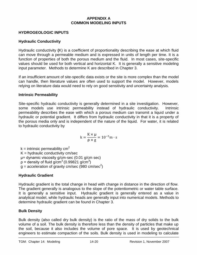
TGM: Chapter 14: Modeling 14-20 Revision 1, November 2007
APPENDIX A COMMON MODELING INPUTS
HYDROGEOLOGIC INPUTS Hydraulic Conductivity Hydraulic conductivity (K) is a coefficient of proportionality describing the ease at which fluid can move through a permeable medium and is expressed in units of length per time. It is a function of properties of both the porous medium and the fluid. In most cases, site-specific values should be used for both vertical and horizontal K. It is generally a sensitive modeling input parameter. Methods to determine K are described in Chapter 3. If an insufficient amount of site-specific data exists or the site is more complex than the model can handle, then literature values are often used to support the model. However, models relying on literature data would need to rely on good sensitivity and uncertainty analysis. Intrinsic Permeability Site-specific hydraulic conductivity is generally determined in a site investigation. However, some models use intrinsic permeability instead of hydraulic conductivity. Intrinsic permeability describes the ease with which a porous medium can transmit a liquid under a hydraulic or potential gradient. It differs from hydraulic conductivity in that it is a property of the porous media only and is independent of the nature of the liquid. For water, it is related to hydraulic conductivity by
k = intrinsic permeability cm2 K = hydraulic conductivity cm/sec μ= dynamic viscosity g/cm-sec (0.01 g/cm sec) ρ = density of fluid g/cm3 (0.99821 g/cm3) g = acceleration of gravity cm/sec (980 cm/sec2)
Hydraulic Gradient Hydraulic gradient is the total change in head with change in distance in the direction of flow. The gradient generally is analogous to the slope of the potentiometric or water table surface. It is generally a sensitive input. Hydraulic gradient is generally entered as a value in analytical model, while hydraulic heads are generally input into numerical models. Methods to determine hydraulic gradient can be found in Chapter 3. Bulk Density Bulk density (also called dry bulk density) is the ratio of the mass of dry solids to the bulk volume of a soil. The bulk density is therefore less than the density of particles that make up the soil, because it also includes the volume of pore space. It is used by geotechnical engineers to estimate compaction of the soils. Bulk density is used in modeling to calculate

TGM: Chapter 14: Modeling 14-21 Revision 1, November 2007
between the volumetric water content and the gravimetric water content, to calculate retardation factors, and is coupled with the particle density to calculate the porosity of a soil. There is no standard method for measuring of bulk density. Most commonly, dry bulk density is measured by taking a sample of known volume, drying it at 105°C for 24 hours or until a constant weight is obtained, then weighing the dried soil sample. The dry weight divided by the volume is the bulk density (Ohio EPA, 2003b). Other methods to measure bulk density include radiation techniques (Blake and Hartge,1986). Site-specific bulk density also can be determined by ASTM D2167-94 (2001), D2922-05, and D2937-04. The dry bulk density will vary within certain limits for different soil types. Range of default values for various media can be found in Table A14.1. In most cases, bulk density is not a sensitive parameter and these values may be used as defaults in models. A sensitivity analysis should be provided unless the model documentation indicates the bulk density is not sensitive. Table A14.1 Bulk Density (Jury,1986). Soil Type Bulk Density
(g/cm3) Sand 1.59 - 1.65 Sandy Loam 1.2 - 1.49 Silt loam 1.47 Clay Loam 1.2-1.36 Silty clay 1.26 Porosity/Effective Porosity Porosity is the ratio of openings to the total volume of rock and soil. The pore space and the arrangement of pore spaces within a soil sample are very complex and difficult to measure. This is because the arrangement of soil particles influences the shape, size and orientation of pores within the soil matrix. The porosity of a soil will vary with the arrangement of particles or texture. In general, finer grained soils, rich in clay, will have the highest porosity, and coarser textured soils, rich in sand, will have lower porosity. Porosity (n) can be calculated by a variety of means. The most common is to calculate the percentage of total soil volume occupied by pores. This is done by calculating a soil’s bulk and particle density (Blake and Heritage, 1986) and using:
Typical porosities are listed in Table 14.2 and in TGM Chapter 3, Table 3.9. On average, particle densities of 2.65 g/cm3 are typical of sandy soils but decrease as the clay and organic matter content rise. Another method is to use pycnometry as described by Danielson and Sutherland (1983). Porosity measurements are important and are used in most ground water and fate and
TGM: Chapter 14: Modeling 14-22 Revision 1, November 2007
transport models. These measurements serve as a basis for determining the water-filled porosity, air-filled porosity and in calculations to determine the total mass of contaminants. Not all of the porosity is available for flow. Part will be occupied by static fluids being held to the soil/rock by surface tension or contained in dead end pore spaces. The porosity available for fluid flow is the effective porosity. It is also a function of the size of the molecules that are being transported to the relative size of the passageways that connect the pores. Therefore, the effective porosity for solute transport may differ from that of water for the same material. Effective porosity is difficult to measure and is typically selected by experience and intuition. Effective porosity is generally estimated based on the description and classification of subsurface materials and by total porosity, determined from lab tests or estimated from the literature. Tables A14.2 and A14.3 provide data that might be useful to this estimation. Peyton et al. (1986) found that even in lacustrine clay, water molecules could pass through all pore throats, so that effective porosity was essentially the same as porosity (Fetter, 2001). This suggests that, for at least water, effective porosity may be considered equal to total porosity. For unfractured glacial till, it is recommended that 30 percent be used for ne in velocity calculations7. While a default value of one percent has been cited for clay (U.S. EPA, 1986), this results in high rates that are intuitively incorrect. Primary flow through clay is known to be very low. This 30% compares favorably with the value for clays reported by Rawls et al. (1983) (Table A14.2). Ohio EPA’s experience is that use of 30 percent results in very conservative estimates of ground water movement through unfractured glacial till.
7It should be noted that the applicability of Darcy’s law to calculating primary flow velocity in fine-grained material is
questionable. However, this currently is one of the best available tools to assist professionals in evaluating whether a
confining unit provides protection to the underlying ground water. To further demonstrate that ground water has not/will
not be affected by a potential contaminant source, other methods such as tracers may be helpful.
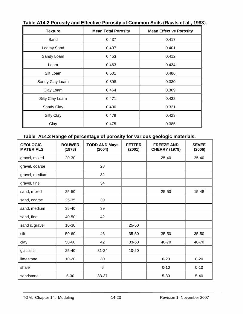
TGM: Chapter 14: Modeling 14-23 Revision 1, November 2007
Table A14.2 Porosity and Effective Porosity of Common Soils (Rawls et al., 1983).
Texture
Mean Total Porosity
Mean Effective Porosity
Sand
0.437
0.417
Loamy Sand
0.437
0.401
Sandy Loam
0.453
0.412
Loam
0.463
0.434
Silt Loam
0.501
0.486
Sandy Clay Loam
0.398
0.330
Clay Loam
0.464
0.309
Silty Clay Loam
0.471
0.432
Sandy Clay
0.430
0.321
Silty Clay
0.479
0.423
Clay
0.475
0.385
Table A14.3 Range of percentage of porosity for various geologic materials.
GEOLOGIC MATERIALS
BOUWER
(1978)
TODD AND Mays
(2004)
FETTER (2001)
FREEZE AND
CHERRY (1979)
SEVEE (2006)
gravel, mixed
20-30
25-40
25-40
gravel, coarse
28
gravel, medium
32
gravel, fine
34
sand, mixed
25-50
25-50
15-48
sand, coarse
25-35
39
sand, medium
35-40
39
sand, fine
40-50
42
sand & gravel
10-30
25-50
silt
50-60
46
35-50
35-50
35-50
clay
50-60
42
33-60
40-70
40-70
glacial till
25-40
31-34
10-20
limestone
10-20
30
0-20
0-20
shale
6
0-10
0-10
sandstone
5-30
33-37
5-30
5-40

TGM: Chapter 14: Modeling 14-24 Revision 1, November 2007
Water Content Water content indicates the amount of water in a soil sample. In the vadose zone, this value will change over time as the soil water budget changes. Most vadose zone models require some measure of water content. However, there is some confusion about the basis for water content measurement and the use of the data. The most common measurement is the percent moisture content of a soil sample. The measurement is made by weighing a soil sample, drying it at 105 C until a constant weight is obtained, then weighing the dried soil sample. The percent moisture content is then:
The ratio of dry weight to wet weight of a soil sample represents the gravimetric water content or water content on a mass basis (θm). Unfortunately, most vadose zone models require that water content of a soil be expressed in terms of volumetric water content (θV). The conversion from water content based upon mass to that of a volumetric basis can be made with the following relationships:
where the bulk density is defined previously and density of water is usually assumed to be 1.0 g/cm3. In many applications, the model prompts the user for neither the volumetric nor mass water content. Instead, it requires water-filled porosity or the percentage that the average pore-space is filled with water. This value can be determined by first noting that:
Rearranging equation 3 in terms of volume of soil and substituting this relation in equation 2, the following relationship is found:
This ratio is then multiplied by 100 to determine the percentage of water in the pore space of a soil sample. For example, if a sample is determined to have 20% moisture content (determined on a mass basis), a dry bulk density of 1.5 g/cm3 , a total porosity of 0.5 (i.e. 50%) and the density of water is 1.0 g/cm3, then:
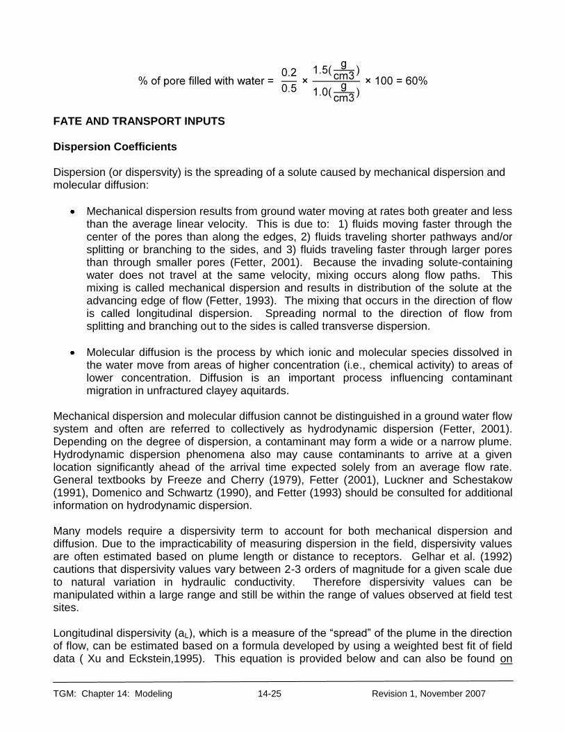
TGM: Chapter 14: Modeling 14-25 Revision 1, November 2007
FATE AND TRANSPORT INPUTS Dispersion Coefficients Dispersion (or dispersvity) is the spreading of a solute caused by mechanical dispersion and molecular diffusion:
Mechanical dispersion results from ground water moving at rates both greater and less than the average linear velocity. This is due to: 1) fluids moving faster through the center of the pores than along the edges, 2) fluids traveling shorter pathways and/or splitting or branching to the sides, and 3) fluids traveling faster through larger pores than through smaller pores (Fetter, 2001). Because the invading solute-containing water does not travel at the same velocity, mixing occurs along flow paths. This mixing is called mechanical dispersion and results in distribution of the solute at the advancing edge of flow (Fetter, 1993). The mixing that occurs in the direction of flow is called longitudinal dispersion. Spreading normal to the direction of flow from splitting and branching out to the sides is called transverse dispersion.
Molecular diffusion is the process by which ionic and molecular species dissolved in the water move from areas of higher concentration (i.e., chemical activity) to areas of lower concentration. Diffusion is an important process influencing contaminant migration in unfractured clayey aquitards.
Mechanical dispersion and molecular diffusion cannot be distinguished in a ground water flow system and often are referred to collectively as hydrodynamic dispersion (Fetter, 2001). Depending on the degree of dispersion, a contaminant may form a wide or a narrow plume. Hydrodynamic dispersion phenomena also may cause contaminants to arrive at a given location significantly ahead of the arrival time expected solely from an average flow rate. General textbooks by Freeze and Cherry (1979), Fetter (2001), Luckner and Schestakow (1991), Domenico and Schwartz (1990), and Fetter (1993) should be consulted for additional information on hydrodynamic dispersion. Many models require a dispersivity term to account for both mechanical dispersion and diffusion. Due to the impracticability of measuring dispersion in the field, dispersivity values are often estimated based on plume length or distance to receptors. Gelhar et al. (1992) cautions that dispersivity values vary between 2-3 orders of magnitude for a given scale due to natural variation in hydraulic conductivity. Therefore dispersivity values can be manipulated within a large range and still be within the range of values observed at field test sites. Longitudinal dispersivity (aL), which is a measure of the “spread” of the plume in the direction of flow, can be estimated based on a formula developed by using a weighted best fit of field data ( Xu and Eckstein,1995). This equation is provided below and can also be found on

TGM: Chapter 14: Modeling 14-26 Revision 1, November 2007
U.S. EPA On-Line Tools for assessing longitudinal dispersivity. (Note: Equation is specific to units (e.g., metric)).
αL = Longitudinal dispersivity (m) Lp = Plume length (m)
Other commonly used relationships for dispersivity include:
(U.S. EPA 1996)
(Gelhar and Axness, 1981)
(Gelhar and Axness, 1981) Where: αL = Longitudinal dispersivity (m)
αv = vertical dispersivity (m) αT = transverse dispersivity (m)
Lp = Plume length (m) Fraction of Organic Carbon The fraction of organic carbon (foc ) is the carbon in the soil that is made up of decaying plant and animal matter, humus, etc. It is differentiated from inorganic carbon (typically in calcium or magnesium carbonates), which does not have the same effect on contaminant movement. The fraction of organic carbon is generally the dominant retarding mechanism for contaminant movement in the vadose zone. Organic carbon and matter contents of soils can have a significant effect on fate and transport; therefore, accurate determination is important and sampling and analysis should be performed with great care. For site-specific modeling, the practitioner should collect a representative number of samples, both horizontally and vertically, over the affected area. Analytical methods to determine organic matter can be found in ASTM D2974-00 or Soil Science Society of America Methods (Nelson and Sommers, 1996). Commonly, modified ground water methods for total organic carbon are used by commercial laboratories and, in general, these methods can overestimate the amount organic carbon in soils. This is because inorganic carbon is not distinguished by the analytical method. The practitioner is directed to the methods of analysis outlined by Nelson and Sommers (1996), which will give an accurate account of soil organic carbon content. Methods such as SW-846 Method 9060A (U.S.EPA, 2004) should not be used to determine the organic carbon content of soils without modification. Additional information can found in VAP TDC document VA30007.03.019 (Ohio EPA,2003a). If site-specific values are not determined, acceptable defaults for sand, silt, and clay are 0.2, 0.25 and 0.3, respectively.

TGM: Chapter 14: Modeling 14-27 Revision 1, November 2007
Partitioning Partitioning is a process in which chemicals are distributed between solid, liquid, and gas phases, depending upon solubility, sorption, and vapor pressure characteristics. Soil Organic Carbon-Water Partitioning Coefficient The soil organic carbon-water partitioning coefficient (KOC ) is the ratio of the mass of a chemical that is adsorbed in the soil per unit mass of organic carbon in the soil per the equilibrium chemical concentration in solution. KOC values are useful in predicting the mobility of organic soil contaminants; higher KOC values correlate to less mobility chemicals, while lower KOC values correlate to more mobility. Koc values can vary greatly in the literature, and a sensitivity analysis may be needed. However, depending on the regulated program, Ohio EPA will generally accept the values listed in Table 3 of the Division of Hazardous Waste Management, Closure Review Guidance (2006), or the Division of Emergency and Remedial Response, Voluntary Action Program, Support Document for Development of Generic Numeric Standards and Risk Assessment (Ohio EPA, 2002).
The coefficients presented in these papers are not applicable for situations where mobilization is from enhanced solvation. The Kd values presented assume that relatively dilute solution conditions are present, that a narrow range of soil moisture content is applicable and that a consistent range of soil organic matter is present. If these basic assumptions are not met, site-specific determination of the leaching of inorganic substances is warranted.
Distribution Coefficient Distribution coefficient (Kd) is the ratio of a chemical's sorbed concentration (mg/kg) to the dissolved concentration (mg/L) at equilibrium. For organics, Kd may be calculated by multiplying Koc (the soil organic carbon-water partitioning coefficient) by the fraction of organic carbon (foc): Kd = Koc x foc For metals, acceptable values for several metals can be found in Table 3 of Ohio EPA’s, Division of Hazardous Waste Management, Vadose Zone Modeling for RCRA Closure (Ohio EPA, 2003b). Relative Solubility Relative solubility controls whether a contaminant exists in ground water primarily as a dissolved (soluble) or free liquid phase (insoluble). Movement of the dissolved phase is generally in the direction of flow and is governed primarily by the processes of advection-dispersion and biological/chemical attenuation. Literature values are generally acceptable for solubility and the values provided in guidance listed under the Koc section are acceptable.

TGM: Chapter 14: Modeling 14-28 Revision 1, November 2007
Henry’s Law Constant At a constant temperature, the amount of a given gas dissolved in a given type and volume of liquid is directly proportional to the partial pressure of that gas in equilibrium with that liquid. Note that care should be taken to determine the units of Henry’s Law constant. Some models require the term to be in m3-atm/mol while other models require it to be dimensionless. Variation of Henry's Law constant can affect model results. The high Henry's Law constant of some volatile organics controls volatilization in the subsurface, dominating other pollutant loss mechanisms. Hence, a slight change may affect the model. However, Henry's Law constants do not vary to a great degree as reported in literature. For ground water and subsurface fate and transport models, acceptable default values are listed in Table 3 of the Division of Hazardous Waste Closure Review Guidance (Ohio EPA, 2006), or the Division of Emergency and Remedial Response, Voluntary Action Program, Support Document for Development of Generic Numeric Standards and Risk Assessment (Ohio EPA, 2002).
Degradation
Degradation of contaminants in the environment can be biotic (biologically mediated) or abiotic (chemical reaction). It accounts for the loss of a pollutant and the formation of daughter products. If the degradation process is accounted for, but not properly justified, predicted concentrations of a pollutant could be underestimated. Likewise, if degradation is occurring, but not accounted for, daughter products, which may be more toxic than the parent compound, may not be properly addressed. Many models incorporate degradation as a first order decay rate. The user is responsible for demonstrating whether degradation is occurring, what degradation products will form, and the significance of the degradation products Literature values for biodegradation rates are highly variable and are often based on laboratory testing or in field conditions where the factors affecting biodegradation can be controlled. The Committee on In Situ Bioremediation1 recommends that the effectiveness of intrinsic bioremediation should be continually monitored by analyzing the fate of the contaminants and other reactants and products indicative of bioremediation. This monitoring includes three types of information: documented loss of contaminants from a site, laboratory assays showing that the microorganisms from site samples have the potential to transform contaminants under the expected site conditions, and confirming evidence that the biodegradation potential is actually realized in the field. Additional information on biodegradation can be found in ASTM E1943-98 (2004), US EPA, (1998), ITRC (1999), and
1 The Committee on In Situ Bioremediation was established in 1992 with the specific task of developing guidelines for evaluating in situ bioremediation projects and determining whether they are or will meet clean-up goals. It represents the span of groups involved in bioremediation: buyers of bioremediation services, bioremediation contractors, environmental regulators, and academic researchers.

TGM: Chapter 14: Modeling 14-29 Revision 1, November 2007
NRC (2000). The user should consult with the regulatory program to determine whether literature values of degradation are acceptable and if so, how they can be applied.1 Source Size Sufficient data needs to be collected to adequately determine or estimate the source or plume size both vertically and spatially. Initial (concentration) Inputs Initializing the plume concentration needs to be assessed. Whether to use the maximum or average may be dependent on the purpose of the model, amount of data, and the complexity of the chosen model. It is recommended that the user consult with the regulatory program to develop an acceptable approach.
1 For RCRA Closures, the Division of Hazardous Waste Management will not accept literature values for biodegradation of organic chemicals. If biodegradation rates are included in a model, site-specific data, including the methods used, number of samples, and laboratory data reports must be supplied to verify these inputs. For DERR/VAP properties see TDC document VA 30007.97.004 (Ohio EPA, 1997).

TGM: Chapter 14: Modeling 14-30 Revision 1, November 2007
APPENDIX A REFERENCES
ASTM D2167-94 (2001) Standard Test Method for Density and Unit Weight of Soil in Place
by the Rubber Balloon Method. American Society of Testing Material Standards. West Conshohocken, Pennsylvania.
ASTM D2922-05 Standard Test Methods for Density of Soil and Soil-Aggregate in Place by
Nuclear Methods (Shallow Depth). American Society of Testing Material Standards. West Conshohocken, Pennsylvania.
ASTM D2937-04 Standard Test Method for Density of Soil in Place by the Drive-Cylinder
Method, American Society of Testing Material Standards. West Conshohocken, Pennsylvania.
ASTM D2974 00. Standard Test Methods for Moisture, Ash, and Organic Matter of Peat and
Other Organic Soils. American Society of Testing Material Standards. West Conshohocken, Pennsylvania.
ASTM E1943-98 (2004). Standard Guide for Remediation of Ground Water by Natural
Attenuation at Petroleum Release Sites. American Society of Testing Material Standards. West Conshohocken, Pennsylvania.
Blake and Hartge,1986. Methods of Soil Analysis. Part 1. Physical and Mineralogical
Methods, Second Edition. 1986. A. Klute ed. Soil Science Society of America. Madison, Wi. 363-375 p.
Bouwer, H. 1978. Groundwater Hydrology. McGraw-Hill Book Company. New York. Danielson, R. E. and P. L. Sutherland. 1986. Chapter 18: Porosity. In A. Klute (editor):
Methods of Soil Analysis. Part 1.Physical and Mineralogical Methods, Second Edition Soil Science Society of America. 443 - 463 p
Domenico, P.A, and F. W. Schwartz, 1990. Physical and Chemical Hydrogeology. John
Wiley and Sons, New York, NY. 824 p Fetter, C.W. 2001. Applied Hydrogeology. Macmillan College Publishing Company. New
York, New York. Fetter, C.W. 1993. Contaminant Hydrogeology. Macmillan Publishing Company. New York,
New York. Freeze, R.A. and J.A. Cherry. 1979. Ground Water. Prentice-Hall Inc. Englewood Cliffs,
N.J. Gelhar, L. W., C. Welty and K. R. Rehfeldt, 1992. A critical review of data on field-scale
dispersion in aquifers, Water Resources Research, 28(7): 1955-1974.
TGM: Chapter 14: Modeling 14-31 Revision 1, November 2007
Gelhar, L.W. and C.J. Axness. 1986. Stochastic Analysis of Macro-Dispersion in Three-Dimensionally Heterogeneous Aquifers. Report No. H-8. Hydraulic Research Program. New Mexico Institute of Mining and technology, Socorro N.M.
Golder Associates (1990) Final Report on Breakthrough and Leachate Compatibility
Testing of Typical Clay Liner Materials, Adams Center Facility, Fort Wayne, Indiana. Prepared for Chemical Waste Management of Indiana, Inc.
ITRC. 1999. Natural Attenuation of Chlorinated Solvents in Groundwater: Principles and
Practices. Interstate Technology and Regulatory Cooperation Workgroup and In Situ Bioremedation Work Team.
Jury, W.A. 1986. Vadose Zone Modeling of Organic Pollutants. S.C Hern and S.M Melancon,
eds., Lewis Publishers, Chelsea, Michigan. Luckner, L. and M. Schestakow. 1991. Migration Process in the Soil and Groundwater
Zone. Lewis Publishers. Chelsea, Michigan Nelson, D.W., and L.E. Sommers. 1996. Chapter 35, Total Carbon, Organic Carbon and
Organic Matter. From Methods of Soils Analysis. Part 3. Chemical Methods. Soil Science Society of America. A. Klute ed. pp.961-1069.
NRC. 2002. Natural Attenuation for Groundwater Remediation. Committee on Intrinsic
Remediation. Water Science and Technology Board. National Academy Press. Washington D.C.
Ohio EPA. 2006. Closure plan review guidance for RCRA facilities. Division of Hazardous
Waste Management, Ohio Environmental Protection Agency. Ohio EPA. 2003a. Sampling and Analysis of Fraction of Organic Carbon (foc) in Soils. VAP
TDC document VA30007.03.019. Division of Emergency and Remedial Response, Ohio Environmental Protection Agency
Ohio EPA, 2003b.-Vadose Zone Modeling for RCRA Closure. Division of Hazardous Waste
Management, Ohio Environmental Protection Agency. Ohio EPA, 2002. Support Document for the Development of Generic Numerical Standards
and Risk Assessment Procedures. Division of Emergency and Remedial Response, Voluntary Action Program. Ohio Environmental Protection Agency.
Ohio EPA. 1997. Use of literature biodegradation rates in property specific fate and
transport modeling. VAP TDC DOC 30007.97.004. Division of Emergency and Remedial Response, Ohio Environmental Protection Agency.
Peyton, G.R., J.P. Gibb, M.H. LeFaivre, J.D. Ritchey, S.L. Burch, M.J. Barcelona. 1986.
Effective Porosity of Geologic Materials. Proceedings of the Twelfth Annual Research Symposium: Land Disposal, Remedial Action, Incineration and Treatment of Hazardous Waste. United States Environmental Protection Agency. EPA/600/9-86/002. pp. 20-28.

TGM: Chapter 14: Modeling 14-32 Revision 1, November 2007
Rawls, W.J.D., L. Brakensiek, and N. Miller. 1983. Green-Amp Infiltration Parameters from Soil Data. ASCE Journal of Hydraulic Engineering. Vol. 9, No. 102.
Sara, M.C. 2003. Site Assessment and Remediation Handbook. Second Edition. CRC
Press, Lewis Publications. pp. Seeve, W.W. 2006. Second Edition. Methods and Procedures for Defining Aquifer
Parameters. In: D. M. Nielsen (editor), Practical Handbook of Environmental Site Characterization and Ground-Water Monitoring. Taylor & Francis Group, LLC. Boca Raton, Florida. Pp. 913-958.
Todd, D.K, and L.W. Mays. 2004. Ground Water. Third Edition. John Wiley and Sons. New
York. U.S. EPA,, 2004. SW-846 Method 9060A, Total Organic Carbon. U.S. EPA. SW-846 On-
Line. Test Methods for Evaluating Solid Waste. U.S. EPA. 1998. Technical Protocol for Evaluating Natural Attenuation of Chlorinated
Solvents in Ground Water. U.S. Environmental Protection Agency. Office of Research and Development. EPA/600/R-98/128
U.S. EPA. 1996. Soil Screening Guidance: Technical Background Document. OSWER.
Washington, D.C. Pub. EPA/540/ R95/128. U.S. EPA, 1986. Criteria for Identifying Areas of Vulnerable Hydrogeology Under the
Resource Conservation and Recovery Act. [Statutory Interpretive Guidance. Guidance Manual for Hazardous Waste Land Treatment, Storage and Disposal Facilities.] Interim Final. Office of Solid Waste and Emergency Response, Washington, D.C.
Xu, M. and Y. Eckstein, 1995. Use of weighted least-squares method in evaluation of the
relationship between dispersivity and field scale, Ground Water, 33(6): 905-908.

State of Ohio Environmental Protection Agency
Division of Drinking and Ground Waters
Technical Guidance Manual for Ground Water Investigations Chapter 15
Use of Direct Push Technologies for Soil and Ground Water Sampling
Geoprobe® Systems
February 2005 Governor : Ted Strickland Director : Chris Korleski
TGM Chapter 15: Direct Push Technologies February 2005 ii
TECHNICAL GUIDANCE MANUAL FOR
GROUND WATER INVESTIGATIONS
CHAPTER 15
USE OF DIRECT PUSH TECHNOLOGIES FOR
SOIL AND GROUND WATER SAMPLING
February 2005
Ohio Environmental Protection Agency Division of Drinking and Ground Waters P.O. Box 1049 55 West Town Street
Columbus, Ohio 43216-1049 Phone: 614-644-2752
http://www.epa.state.oh.us/ddagw/
TGM Chapter 15: Direct Push Technologies February 2005 iii
PREFACE
This document is part of a series of chapters incorporated in Ohio EPA’s Technical Guidance Manual for Hydrogeologic Investigations and Ground Water Monitoring (TGM), which was originally published in 1995. DDAGW now maintains this technical guidance as a series of chapters rather than as an individual manual. These chapters can be obtained at http://www.epa.state.oh.us/ddagw/tgmweb.aspx. The TGM identifies technical considerations for performing hydrogeologic investigations and ground water monitoring at potential or known ground water pollution sources. The purpose of the guidance is to enhance consistency within the Agency and inform the regulated community of the Agency’s technical recommendations and the basis for them. In Ohio, the authority over pollution sources is shared among various Ohio EPA divisions, including the Emergency and Remedial Response (DERR), Hazardous Waste Management (DHWM), Solid and Infectious Waste (DSIWM), and Surface Water (DSW), as well as other state and local agencies. DDAGW provides technical support to these divisions. Ohio EPA utilizes guidance to aid regulators and the regulated community in meeting laws, rules, regulations, and policy. Guidance outlines recommended practices and explains their rationale. The Agency may not require an entity to follow methods recommended by this or any other guidance document. It may, however, require an entity to demonstrate that an alternate method produces data and information that meet the pertinent requirements. The procedures used usually should be tailored to the specific needs and circumstances of the individual site, project, and applicable regulatory program, and should not comprise a rigid step-by-step approach that is utilized in all situations.

TGM Chapter 15: Direct Push Technologies February 2005 iv
ACKNOWLEDGMENTS
This guidance was developed by Ohio EPA's Division of Drinking and Ground Waters (DDAGW). The following people are acknowledged for the preparation of this document.
Primary author: Sydney Poole, DDAGW-CO, who had primary responsibility for researching and writing the document. Additional writing and editing was provided by the members of the Ohio EPA Direct Push Technologies Workgroup. Personnel who contributed to the DPT Workgroup include: Eric Schultz, DHWM-CO; Joe Jellick, DEFA,-CO (formerly of DERR, CO); Karl Reinbold, DERR-CO; Matt Justice; DERR-SWDO (formerly of DDAGW, SWDO); and Erik Hagen, DHWM-CO.
Editor: Jeff Patzke, DDAGW-CO, who served as editor and project coordinator of the Technical Guidance Manual.
The Ohio EPA would also like to thank the numerous people who provided input on the document during its developmental stages. The comments and recommendations of DDAGW-District Offices, and other Ohio EPA Divisions, State and Federal Agencies, private consultants, and regulated community were greatly appreciated.

TGM Chapter 15: Direct Push Technologies February 2005 v
TABLE OF CONTENTS PREFACE .................................................................................................................. 15-iii TABLE OF CONTENTS ............................................................................................. 15-v EQUIPMENT FOR ADVANCING DPT RODS ............................................................ 15-2
SINGLE TUBE (SINGLE ROD) ............................................................................. 15-2 TWO TUBE (CASED, DUAL TUBE) ...................................................................... 15-2
SOIL SAMPLING ....................................................................................................... 15-5 Open Solid Barrel Samplers ............................................................................ 15-5 Split Barrel Samplers (Split Spoon Samplers) ................................................. 15-5 Thin-Walled Tube Samplers (Shelby Tubes) ................................................... 15-5
CLOSED BARREL SAMPLERS (PISTON SAMPLERS) ....................................... 15-6 SOIL SAMPLING METHOD EVALUATION .......................................................... 15-7
Single Tube Sampling Considerations ........................................................... 15-7 Two Tube Sampling Considerations .............................................................. 15-8 Soil Sampling Recommendations .................................................................. 15-8
GROUND WATER SAMPLING .................................................................................. 15-9 GROUND WATER GRAB SAMPLERS ................................................................. 15-9
Exposed Screen Samplers ........................................................................... 15-9 Closed Screen Samplers ............................................................................ 15-11 Ground Water Profilers ............................................................................... 15-11
DPT INSTALLED WELLS ................................................................................... 15-13 Conventionally Screened and Packed Wells ............................................. 15-13 Pre-Packed Screen Wells .......................................................................... 15-13 Development of DPT ................................................................................. 15-15 Probehole and Monitoring Well Sealing ..................................................... 15-15
GROUND WATER SAMPLING METHOD EVALUATION ................................... 15-17 Grab Samplers .......................................................................................... 15-17 Wells ................................................................................................. 15-18
APPLICATIONS OF DPT FOR GROUND WATER SAMPLING ......................... 15-19 Considerations for Use as a Screening Tool ............................................ 15-19 Considerations for Collection of Compliance Samples ............................. 15-19
SPECIALIZED MEASUREMENT AND LOGGING TOOLS ................................. 15-20 GEOTECHNICAL ................................................................................................ 15-21 GEOPHYSICAL ................................................................................................... 15-21 HYDROGEOLOGICAL ........................................................................................ 15-22 ANALYTICAL ...................................................................................................... 15-22 SOIL GAS SAMPLING ........................................................................................ 15-23
Soil Gas Samplers ................................................................................... 15-23 Retrieving Soil Gas Samples .................................................................... 15-24
REFERENCES ......................................................................................................... 15-25

TGM Chapter 15: Direct Push Technologies February 2005 1
USE OF DIRECT PUSH TECHNOLOGIES
FOR SOIL AND GROUND WATER SAMPLING Direct push technology (DPT) devices are investigation tools that drive or push small-diameter rods and tools (typically not exceeding four inches in diameter) into the subsurface by hydraulic or percussive methods. Direct push can be used for a number of applications. Specialized direct push probes may be used to collect in-situ geophysical, geochemical, and geotechnical measurements. Applications include soil sampling, ground water sampling, geophysical sensing, geochemical sensing, and soil gas sampling. The purpose of this guidance document is to discuss the applications of direct push to soil and ground water sampling. DPT tools such as the cone penetrometer have been used for assessing site geology for many years. With the invention of the Hydropunch(TM) in 1988, (Edge and Cordry, 1989) an alternative to monitoring wells for collecting ground water samples was developed. DPT technology became more popular in the 1990's in response to a growing need to assess sites more quickly and cheaply. A growing number of inquiries from the public about DPT during this time prompted Ohio EPA to form a Direct Push Technologies Workgroup in June of 1998 to evaluate DPT as they relate to site characterization. Depending on site conditions, DPT methods may offer an attractive alternative to traditional sampling methods such as hollow stem augering with split spoon sampling. Advantages include the smaller size of the DPT rigs, which allows for sampling in spaces that would be impossible for larger, conventional hollow stem auger (HSA) rigs; and quicker penetration, allowing for more efficient and economical site characterization. DPT also produces fewer cuttings, and the smaller diameter holes require fewer materials for well installation or probehole sealing. An additional benefit is that a minimal amount of waste material is produced when compared to traditional drilling methods. The speed and mobility advantages of DPT soil sampling may allow a more complete and accurate investigation of site geology. Similarly, when investigating ground water, the speed of investigation and a lack of a need for well materials may allow for a more thorough characterization of the hydrogeology of the site. Purge water disposal volumes are smaller, since the volume of water extracted during well development and purging is much less than it would be for a conventionally installed well due to the smaller radius of disturbed aquifer around the well.
DPT is applicable in unconsolidated sediments. It is most applicable for shallow depths (less than 100 feet), but may be able to go deeper depending on site conditions. Because of the lighter weight and therefore limited downward force, penetration may be difficult in sediments containing a high percentage of gravels and cobbles or in dense, highly compacted sediments (such as overconsolidated till). Alternative drilling methods may be advisable in situations of unfavorable conditions. This paper addresses the use of DPT in the applications of both stratigraphic investigations and chemical analysis. The primary sources of information for this document include: ASTM Method D6282-98; EPA (1997); ASTM Method D6001-98(2002); ASTM Method D6724-04; ASTM Method D6725-01; and the draft EPA guidance Groundwater Sampling

TGM Chapter 15: Direct Push Technologies February 2005 2
and Monitoring with Direct Push Technologies (draft). The knowledge and experience of the DPT Workgroup members are also reflected.
EQUIPMENT FOR ADVANCING DPT RODS DPT devices may be driven by manual, mechanical, or hydraulic methods, and may be truck-mounted or stand-alone. A DPT tool string includes the sample collection tool and extension rods for advancement and retrieval of the sample tool. There are two types of rod systems: 1) single tube and 2) two tube. Both allow for soil, soil gas, and ground water sampling. Single and two tube systems have overlapping applications and can be used in many of the same environments. However, there are strengths and limitations associated with each that should be considered. SINGLE TUBE (SINGLE ROD) Single tube rod systems are the most commonly used. They use a single string of rods to connect the probe or sampling tool to the rig. The rod diameters are smaller than the sampler, typically around one inch, but may range from 0.5 to 2.125 inches. Once a sample has been collected, the entire string must usually be removed from the probe hole. If subsequent sample collection at greater depths is required, the process must be repeated by re-entering with an empty sampler. Figure 15.1 shows a visual representation of this process. TWO TUBE (CASED, DUAL TUBE) Two tube rod systems advance two sections: an outer tube, or casing, and a separate inner rod with the sampler attached (Figure 15.2). The outer tube is used for stabilization. The inner tube is used for sampler recovery and insertion. Because two tubes are advanced, outer tube diameters are relatively large, typically 2.4 inches; however, they can range between 1.25 and 4.2 inches. The outer casing and inner extension rod with sampler are advanced simultaneously for the length capacity of the sampler. The sampler is removed from the probehole and a new sample barrel or plug bit is inserted for each increment of depth. Because the hole is cased, continuous sampling is simplified and expedited. Withdrawing the tool string from the probehole is accomplished by applying a retractive force on the tool string assembly. The drill string can either be withdrawn by direct mechanical pull through use of a hydraulic system, or by line-pull using mechanical or hydraulic powered winches or cathead and rope windlass type devices. The drill string can also be retracted by back-pounding using weights. However, back-pounding can cause disturbances to the sample and should be avoided.

TGM Chapter 15: Direct Push Technologies February 2005 3
Figure 1: Figure of a typical open ended sampling device used for continuous coring (from Geoprobe® Systems, 1997)
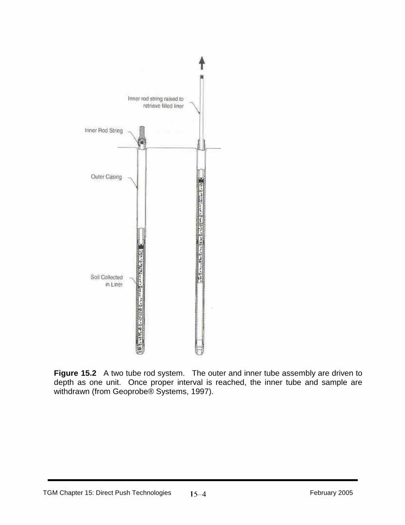
TGM Chapter 15: Direct Push Technologies February 2005 4
Figure 15.2 A two tube rod system. The outer and inner tube assembly are driven to depth as one unit. Once proper interval is reached, the inner tube and sample are withdrawn (from Geoprobe® Systems, 1997).

TGM Chapter 15: Direct Push Technologies February 2005 5
SOIL SAMPLING There are two types of DPT soil samplers: 1) open barrel and 2) closed barrel. Open barrel samplers remain open as they are pushed to the target depth. Closed barrel samplers remain closed until reaching the target depth. The primary sources of information on soil sampling used in this document may be found in ASTM Method D6282-98 and EPA (1997). OPEN BARREL SAMPLERS These samplers have an open end allowing material to enter at any time or depth (Figure 15.1). They may also be referred to as unprotected or unsealed samplers. The three most commonly used open barrel samplers are: 1) open solid barrel; 2) split barrel (or split spoon); and 3) thin-walled. Available sampler lengths range from one to five feet. Split barrel and thin-walled samplers are also commonly used with hollow stem augers. They are discussed at greater length in “Drilling and Subsurface Sampling”, Chapter 6 of the Technical Guidance Manual for Hydrogeologic Investigations and Ground Water Monitoring (Ohio EPA, 1995). Open Solid Barrel Samplers Open solid barrel samplers consist of a head assembly, a barrel, and a drive shoe. The sampler is attached to the DPT rods at the head assembly. A check valve, which allows air or water to escape as the barrel fills with soil, is located within the head assembly. The check valve improves the amount of soil recovered in each sample by allowing air to escape. With the use of liners, samples can be easily removed for volatile organic compound (VOC) analysis or for observation of soil structure. Split Barrel Samplers (Split Spoon Samplers) Split barrel samplers, also often used with hollow stem augers, are similar to open solid barrel samplers except that the barrels are split longitudinally so that the sampler can be easily opened. The primary advantage of split barrel samplers is that they allow direct observation of soil cores without the use of liners and without physically extruding the soil core. As a result, split-barrel samplers are often used for geologic logging. Split barrel samplers, however, may cause more soil compaction than open solid barrel samplers because the tool wall thickness is often greater. Although liners are not compatible with all split barrel samplers, they may be used to reduce the need for decontamination. Additional information on the use of split spoon samplers with hollow stem augers may be found in “Drilling and Subsurface Sampling”, Chapter 6 of the Technical Guidance Manual for Hydrogeologic Investigations and Ground Water Monitoring (Ohio EPA, 1995). Thin-Walled Tube Samplers (Shelby Tubes) Thin-walled tube samplers, similar to larger diameter samplers known as Shelby tubes, are used with both DPT and hollow stem augers for collecting undisturbed samples. The sampling tube is typically attached to the sampler head using recessed cap screws or rubber expanding bushings. The sampler walls, made of thin steel with a sharpened cutting edge,

TGM Chapter 15: Direct Push Technologies February 2005 6
minimize soil compaction compared to other types of samplers. Relatively undisturbed samples are required for certain geotechnical analyses such as permeability and triaxial shear tests. More information on the use of thin wall samplers may be found in “Drilling and Subsurface Sampling”, Chapter 6 of the Technical Guidance Manual for Hydrogeologic Investigations and Ground Water Monitoring (Ohio EPA, 1995). CLOSED BARREL SAMPLERS (PISTON SAMPLERS) Piston samplers are the only type of closed barrel soil sampler currently available (Figure 15.3). They are similar to open solid barrel samplers, except that the opening is sealed with a rigid, pointed piston that displaces soil as it is advanced. When the sampler has been pushed to the desired depth, the piston is unlocked by releasing a retaining device, and subsequent pushing or driving forces soil into the sampler. The assembly can then be removed and soil extracted. Piston samplers are typically air and water tight; however, if o-ring seals are not maintained, leakage may occur. Piston samplers also have the advantage of increasing the recovery of unconsolidated sediments as a result of the relative vacuum that is created by the movement of the piston.
Figure 3: Figure of a typical closed barrel sampling device used for discrete depth sampling (from Geoprobe® Systems, 1997).

TGM Chapter 15: Direct Push Technologies February 2005 7
SOIL SAMPLING METHOD EVALUATION DPT offers many advantages for soil sampling, including fast site assessment, rig mobility, and greater efficiency than conventional drilling methods. Use of available sampler lengths of up to five feet can allow for more continuous sampling intervals than are possible with conventional split-spoon samplers. In general, DPT is applicable in unconsolidated sediments that are conducive to withdrawing sufficient soil volume for analysis. A discussion of what should be considered when determining whether to use a single tube or two tube sampler follows. Where sample quality or quantity may not meet sampling objectives, alternatives such as switching to a different sampling method (e.g., hollow stem auger), or a different sampling tool (e.g., a wider diameter sampler) should be employed. Single Tube Sampling Considerations Because only one string of rods is used, single tube systems are not as heavy as two tube systems and enable quicker rod connection. Because of the lightweight rod string, situations in which a single sample is desired or with shallow sampling depths can be sampled quickly and easily with few complications. However, the lack of hole casing can cause some complications when continuous sampling to greater than ten feet is desired. Sampling with single tube rods can be slower because the probe hole may collapse or slough without the stabilization of an outer casing rod. A second drawback of single tube systems is the potential for formation or saturated zone cross contamination during continuous sampling. Because the probe hole is uncased during rod retraction and reinsertion, the open probe hole can serve as a conduit for potentially contaminated soils or ground water from overlying zones that may slough or migrate to otherwise uncontaminated lower zones. Cross contamination is of particular concern if NAPLs (non-aqueous phase liquids) are present that could migrate down the probe hole. Also, when multiple samples are taken, repeated entry can deform or skew the alignment of the probehole. This can create problems when sealing the probehole if a skewed hole prevents complete insertion of a tremie pipe or permits bridging of bentonite pellets or granules. With no outer casing in place to guard the sampler during rod reinsertion, sample biasing may be exacerbated by probehole collapse, probe hole sloughing, or probe hole smearing. Thus, the sampler may collect soil samples from varying zones as it is advanced to the target depth. If the displaced material is contaminated or contains analytes at levels higher than the target depth, the target sample may be biased high. Conversely, if the collapsed material is cleaner or contains analytes at concentrations lower than the target depth, the target sample may be biased low. In either case, the sample collected is not representative of the target depth. Depending on site conditions, the collection of undisturbed samples using thin-walled samplers with DPT may or may not be feasible. Typically, DPT rigs are mounted on lighter trucks than HSA rigs, and do not have hydraulic systems that are capable of generating as much downward force as HSA rigs. Consequently, HSA rigs are better equipped to push thin-walled sample tubes over a wider range of soil condition than DPT rigs.

TGM Chapter 15: Direct Push Technologies February 2005 8
Two Tube Sampling Considerations The use of the outer casing in a two-tube system has several advantages. Two tube systems are faster than single rod systems for continuous sampling at deeper sampling depths (i.e., depths below ten feet). Because only the inner sample barrel is removed, and not the entire rod string, reaching the target depth is not complicated by probe hole sloughing and collapse. In addition, the outer casing maintains the probe hole's alignment during multiple insertions of the sampling rod. This helps assure a proper grout seal. Because the outer casing is never removed during sampling, the probe hole remains sealed, reducing the potential for sloughing of contaminated soil or migration of contaminated fluids down the hole. The outer casing also protects non-sealed samplers from sample biasing caused by smearing. In addition, the outer casing enables the use of non-sealed samplers for vertical contaminant profiling above the saturated zone. Use of the outer casing in a two-tube system also has disadvantages. It is heavier, requiring twice as much rod and a heavier rig, thus making it more cumbersome and more expensive to use. The two tube system is also more susceptible to soil friction because of its larger diameter, slowing boring and sampling. An oversized drive shoe is sometimes used to reduce friction and buckling but may increase the risk of contamination migration down the probehole. Even using heavier driving equipment, penetration depths are often not as great as those possible with single rod systems due to the increased friction. Soil Sampling Recommendations DPT is appropriate for soil sampling when:
· Its use and methodologies are consistent with the data quality objectives of the sampling program.
· Unconsolidated sediments are to be sampled. · Materials to be sampled contain a low percentage of gravel and cobbles and are not
dense or highly compacted. · Materials to be sampled are less than 100 feet in depth. DPT may be able to probe
deeper in some circumstances. If using DPT:
· Two tube sampling should be used whenever possible. This is especially important if NAPLs are present, or if there is a potential for sloughing to a lower zone. If a single tube is used for vertical profilers, it is imperative that sealed samplers are used.
· Closed barrel samplers should be used for most applications. The only situation
where non-sealed samplers would be acceptable is with single sample collection events above the saturated zone.
· If recovery of samples or cave-in of the probehole is problematic, the data quality
objectives should be supplemented or different sampling techniques employed.

TGM Chapter 15: Direct Push Technologies February 2005 9
· Probeholes should be sealed using retraction grouting with a tremie tube and a liquid
slurry material. However, surface pouring may be appropriate for shallow probeholes (less than 10 feet deep) in cohesive formations.
GROUND WATER SAMPLING There are two common types of ground water sampling equipment used in DPT methods: tools for obtaining one-time grab samples, and wells installed using DPT for short-term or long-term sampling. Most sampling devices used with DPT tools are composed of stainless steel or other inert metals. Well screen materials may be composed of stainless steel, polyvinyl chloride, polyethylene, or polytetrafluoroethylene. The primary sources of information on ground water sampling used in this document are ASTM Method D6001-98(2002), ASTM Method D6724-04, ASTM Method D6725-01 and the draft EPA guidance Groundwater Sampling and Monitoring with Direct Push Technologies (draft).
GROUND WATER GRAB SAMPLERS DPT ground water sampling tools are of three basic types: exposed screen samplers, closed screen samplers, and ground water profilers. Exposed Screen Samplers Exposed screen samplers, sometimes referred to as mill-slotted well point samplers, consist of a well screen that allows the influx of ground water and a riser pipe that allows the extraction of a sample. In practice, exposed screen samplers are driven to the approximate sample depth below the ground surface. A ground water sample is taken by extracting water with either a bailer or tubing/pump combination. This necessitates purging and development prior to sampling. A typical exposed screen sampling assembly is shown in Figure 15.4. Because the exposed screen can be pushed to different depths, exposed point samplers have an advantage in taking multi-level water samples without having to remove the tool string. This can be a significant time saving, especially where three-dimensional plume mapping is a data quality objective. Exposed screen samplers may have significant disadvantages. Clogging of the well screen can occur when probing through silty or clay-rich soils as well as with ground water high in suspended solids. For this reason, they are commonly used in geologic formations composed of sands and gravels. If soil is contaminated above the saturated zone of interest, draw-down by the tool string and/or sloughing of contaminated soil produce false-positive results. In addition, contaminated ground water trapped in the well point bore can also be drawn from one zone to another, potentially biasing sampling results at the point of interest. The initial ground water withdrawn from the sampler can be turbid because of the disturbance of the formation while using DPT tools. In addition, because of the small screen diameter, development of the formation can be difficult.

TGM Chapter 15: Direct Push Technologies February 2005 10
Figure 15.4 Diagram of a typical exposed screen sampler (Source: Aller et al., 1991)

TGM Chapter 15: Direct Push Technologies February 2005 11
Closed Screen Samplers Closed screen samplers (Figure 15.5) are protected, sealed sampling devices consisting of a well screen housed within a protective sheath to which are attached an expendable drive point, drive rod(s), and drive head. The assembly is initially driven with the outer casing in place. Rubber O-rings keep the device water tight, eliminating the threat of formation fluids entering the screen before deployment and assuring sample integrity. Once the desired depth is reached, the outer casing is retracted to expose the screen to formation water. After a sample is obtained, the expendable drive point is left in place and the sampling assembly is removed. Screen length can vary from one to five feet. Since the screen is only exposed after the tool has been placed at the target depth, susceptibility of the screen to clogging is reduced. The O-ring seals make the sampler water tight and reduce the likelihood of cross-contamination. In addition, closed screen samplers can be configured to leave the screen and riser in place as a temporary monitoring device. Turbid samples may be caused both by the disturbance of the formation while driving DPT tools, and by the high initial entrance velocity of water into the sampler before the water level inside the sampler reaches equilibrium with the formation water. As with exposed screen samplers, development of the formation can be difficult due to the small screen diameter. A problem can also occur if the screen remains within the outer casing when it is retracted, and therefore fails to be exposed to the formation and ground water. Ground Water Profilers In situations where discrete vertical profiling is desired, a ground water profiler may be used. The profiler is used to detect vertical variations in contaminant concentrations at a single location. Like an exposed screen sampler, a ground water profiler has sampling portholes or a screen through which samples are taken. The profiler is pushed to the desired sampling depth, and a probe rod is used to knock out the expendable drive point. A sample is taken with a peristaltic or other small diameter pump through a tube positioned within the screened area. Once the sample is taken, the sampler may be advanced to the next sampling depth. To prevent plugging of the screen or sampling portholes, the pumping direction of the pump may be reversed and a small amount of water injected into the screen to maintain a positive pressure on the screen and prevent clogging of the sampling ports. Only clean, potable water of known chemical quality transported from off-site should be used. The pump flow is again reversed once the next sampling depth is reached, and another ground water sample is taken from that depth. Once all samples are taken, the probehole may be sealed by pumping grout through the profiler. Figure 15.6 shows a typical ground water profiler assembly. Quick, easy vertical contaminant profiling is available with a ground water profiler. Similar to exposed screen samplers, ground water profilers can take multi-level water samples without having to remove the tool string, thus providing a quick and efficient way of obtaining three-dimensional plume mapping. Ground water profilers have an advantage over exposed screen samplers, however, in that pumping water into the sampler can reduce or eliminate soil clogging of the screen.

TGM Chapter 15: Direct Push Technologies February 2005 12
Figure 15.5 Typical closed screen sampler assembly (from Geoprobe® Systems 2001.

TGM Chapter 15: Direct Push Technologies February 2005 13
Whenever multiple depths are sampled, there is a possibility of drawing contamination to deeper depths that could potentially bias results. While pumping water into the screen during driving may decrease the chances of this happening, the practice can create some problems of its own. Even though the water is pumped into the sampler under low pressure, some water may be introduced into the formation. Alternatively, when the next sample is withdrawn, the clean water may mix with the formation water and cause samples to be biased low. Care should be taken to note the volume of water pumped into the sampler to ensure that the same volume of water is withdrawn. In addition, because of the small diameter and because multiple samples are obtained from one pushing event, it is unlikely that the formation can be sufficiently developed prior to obtaining the sample. DPT INSTALLED WELLS
DPT used for advancing probe rods can be adapted to install wells for long- and short-term monitoring of ground water. The preferred and most common approach is to push the probe rods or the drive casing to the desired depth with a sacrificial tip. The screen and well casing are usually inserted into the rods or drive casing to the total depth. This protects the screen from becoming plugged with soil and being exposed to any overlying zones of contamination. ASTM (2002) provides additional guidance on DPT well installation. Conventionally Screened and Packed Wells
The inside diameter of probe rods or temporary drive casings used for DPT well installations range from 1 ½ to 3 ½ inches. Wells can be installed using conventional well casings and screens with inside diameters up to 2 inches, provided the well can be properly packed and sealed. If the screen is installed in non-cohesive formation material, it may collapse around the screen as the rods or outer casing are removed, eliminating the need for placement of the filter pack. If the formation is stable or cohesive soil, filter pack material may be placed around the screen by pouring it into the annular space between the rod or casing string as the sections are pulled from the hole. The well is sealed by pouring granular bentonite into the annular space or pumping a bentonite slurry through tubing that has been run to the top of the filter pack. The well is grouted from the bottom up by pumping a cement-bentonite slurry through the tubing as the outer string and tubing are removed from the hole. Pre-Packed Screen Wells Wells can also be installed using pre-packed well screens, which help to eliminate problems with small diameter wells in the placement of filter pack around the screen (Figure 15.7). A pre-packed screen is an assembly consisting of an inner slotted screen surrounded by a wire mesh sleeve that acts as a support for filter media. The pre-packed screen assemblies can either be shipped with filter media already packed within the mesh sleeve or can be shipped without filter media and packed with filter sand in the field. Refer to ASTM D5092-02 for appropriate sizing of filter pack material. The wells are sealed and grouted using same procedure described for conventionally completed DPT wells. ASTM D6725 (2002) provides additional guidance on the use of pre-packed wells.

TGM Chapter 15: Direct Push Technologies February 2005 14
Figure 15.6 Typical ground water profiler assembly from Geoprobe® Systems, 2002).

TGM Chapter 15: Direct Push Technologies February 2005 15
Development of DPT Wells Due to the effects of DPT installation on the soils around the well, development of each well is usually needed to ensure sample representativeness. Development of DPT wells helps repair damage done to the formation during the driving of DPT tools, and increases the hydraulic communication between the well and the formation. More information regarding monitoring well development may be found in Chapter 8 of the Technical Guidance Manual for Hydrogeologic Investigations and Ground Water Monitoring (Ohio EPA, 1995). Due to the small casing diameters, the equipment available to develop small diameter wells is limited to small capacity bailers, inertial pumps, and small diameter bladder pumps. Field parameters, including turbidity and draw down, should be monitored during development to determine when the formation and ground water have stabilized. ASTM D 6725-01 (Standard Practice for Direct Push Installation of Prepacked Screen Monitoring Wells in Unconsolidated Aquifers) suggests the use of an inertial lift (or check valve) pump to both surge and purge the formation as an effective method for developing small diameter wells. The downward stroke of the inertial lift pump provides a surging of the water column and loosens the fines in the formation. The following upward stroke of the pump simultaneously removes the loosened fines, preventing them from clogging the screen. However, in finer grained formations, over surging should be avoided to prevent clogging the screen with fines (ASTM D 6725-01). It may be necessary to perform additional purging with a non-surging pumping device to attain lowered turbidity levels for wells installed in fine-grained formations (ASTM D 6724-04). Probehole and Monitoring Well Sealing Because any open hole can act as a conduit for contaminants to the subsurface, all probeholes should be appropriately sealed and abandoned. Due to the small diameter of DPT probeholes, sealing the probeholes offers a few special challenges. It is important to select appropriate sealing methods based on the site-specific conditions, such as position relative to the water table, presence or absence of NAPL, or risk of sloughing. An inadequately sealed probehole or monitoring well can create a preferential pathway for the infiltration of contaminants to previously uncontaminated zones. The procedures for borehole sealing in Chapters 9 of the Technical Guidance Manual for Hydrogeologic Investigations and Ground Water Monitoring (Ohio EPA, 1995) should be followed for all probehole sealing. Additional information about the methods discussed below may be obtained from U.S. EPA (1997). Grouting machines are available for use with small diameter wells that allow the operator to properly seal monitoring well installations and seal soil and ground water sample holes. The use of grouting machines reduces problems of grout bridging and incomplete seals associated with adding grouting materials from the ground surface.
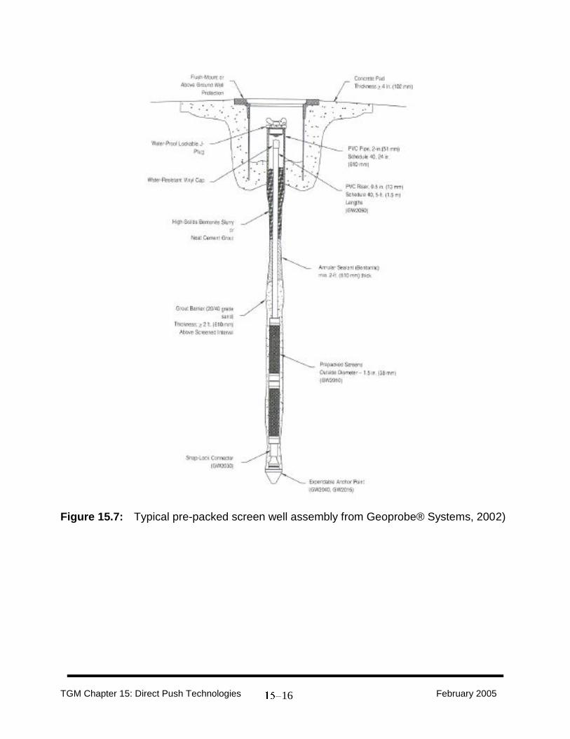
TGM Chapter 15: Direct Push Technologies February 2005 16
Figure 15.7: Typical pre-packed screen well assembly from Geoprobe® Systems, 2002)

TGM Chapter 15: Direct Push Technologies February 2005 17
GROUND WATER SAMPLING METHOD EVALUATION The various types of ground water samplers and wells that are used with DPT are evaluated in the following sections. Grab Samplers With respect to site screening investigations in which ground water samples are not being collected for compliance purposes, grab samplers (closed screen, open screen, and ground water profilers) may delineate site-wide hydrogeology more quickly and efficiently than monitoring wells. Because they are easy to use and do not require well materials, grab samplers typically have a significant advantage over traditional monitoring wells as site screening tools. In addition, they often facilitate hydrogeological evaluation and plume mapping, and can be very helpful in optimizing the location and construction of permanent monitoring wells. Conversely, with respect to obtaining representative ground water samples that generate accurate and verifiable data, the use of grab samplers does present a few challenges. Correct placement of the screened interval is particularly important given the short screen and discrete sampling interval, so that contaminant layers are not missed. The short time frame of many DPT investigations is often insufficient for adequate well development and equilibration with the surrounding formation water. Because there is no filter pack installed around a DPT sampling tool, fines may clog the well screen when sampling in fine-grained formations, preventing ground water from reaching the sampler. Also, the lack of a bentonite seal may allow VOCs to off gas into the atmosphere from the ground water zone if the vadose zone/surficial materials are relatively cohesive and the annular space has not collapsed. Clogging of the screen could cause samples to be biased lower than actual contaminant concentrations. Problems with turbidity may arise due to the inability to adequately develop the sampler. Finally, when sampling objectives include trend analysis and monitoring of remediation efforts as goals, the one-time sampling inherent in samples taken with DPT tools is often not appropriate for these monitoring requirements. When a closed screen sampling tool is opened for sampling, the entrance velocity of water into the screen can be high due to the hydraulic head of the formation water. This initial high entrance velocity can induce degassing of the sample as well as turbidity. Because of these concerns, significant purging of the sampler and the sampling zone should be performed before sampling to reduce bias. As a general rule, multi-level sampling can be accomplished only with repeated advances of a sealed-screen sampler, especially when using a single-tube rod system. Since the probehole must stay open between advances of the sampler, cross-contamination may be a problem between sampling events. Sealed-screen samplers used within a cased/two-tube rod system can eliminate the problems with cross-contamination when multi-level sampling. However, even when using tools that reduce the potential for cross-contamination, all sampling equipment should be decontaminated between sampling intervals. Ground water profilers solve the problem of screen clogging by pumping water into the screen during advancement. This makes ground water profilers an ideal choice when
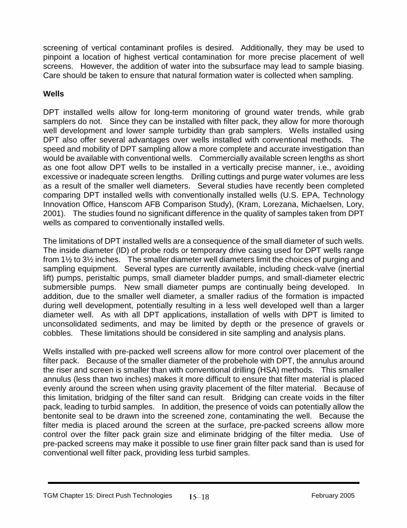
TGM Chapter 15: Direct Push Technologies February 2005 18
screening of vertical contaminant profiles is desired. Additionally, they may be used to pinpoint a location of highest vertical contamination for more precise placement of well screens. However, the addition of water into the subsurface may lead to sample biasing. Care should be taken to ensure that natural formation water is collected when sampling. Wells DPT installed wells allow for long-term monitoring of ground water trends, while grab samplers do not. Since they can be installed with filter pack, they allow for more thorough well development and lower sample turbidity than grab samplers. Wells installed using DPT also offer several advantages over wells installed with conventional methods. The speed and mobility of DPT sampling allow a more complete and accurate investigation than would be available with conventional wells. Commercially available screen lengths as short as one foot allow DPT wells to be installed in a vertically precise manner, i.e., avoiding excessive or inadequate screen lengths. Drilling cuttings and purge water volumes are less as a result of the smaller well diameters. Several studies have recently been completed comparing DPT installed wells with conventionally installed wells (U.S. EPA, Technology Innovation Office, Hanscom AFB Comparison Study), (Kram, Lorezana, Michaelsen, Lory, 2001). The studies found no significant difference in the quality of samples taken from DPT wells as compared to conventionally installed wells. The limitations of DPT installed wells are a consequence of the small diameter of such wells. The inside diameter (ID) of probe rods or temporary drive casing used for DPT wells range from 1½ to 3½ inches. The smaller diameter well diameters limit the choices of purging and sampling equipment. Several types are currently available, including check-valve (inertial lift) pumps, peristaltic pumps, small diameter bladder pumps, and small-diameter electric submersible pumps. New small diameter pumps are continually being developed. In addition, due to the smaller well diameter, a smaller radius of the formation is impacted during well development, potentially resulting in a less well developed well than a larger diameter well. As with all DPT applications, installation of wells with DPT is limited to unconsolidated sediments, and may be limited by depth or the presence of gravels or cobbles. These limitations should be considered in site sampling and analysis plans. Wells installed with pre-packed well screens allow for more control over placement of the filter pack. Because of the smaller diameter of the probehole with DPT, the annulus around the riser and screen is smaller than with conventional drilling (HSA) methods. This smaller annulus (less than two inches) makes it more difficult to ensure that filter material is placed evenly around the screen when using gravity placement of the filter material. Because of this limitation, bridging of the filter sand can result. Bridging can create voids in the filter pack, leading to turbid samples. In addition, the presence of voids can potentially allow the bentonite seal to be drawn into the screened zone, contaminating the well. Because the filter media is placed around the screen at the surface, pre-packed screens allow more control over the filter pack grain size and eliminate bridging of the filter media. Use of pre-packed screens may make it possible to use finer grain filter pack sand than is used for conventional well filter pack, providing less turbid samples.

TGM Chapter 15: Direct Push Technologies February 2005 19
APPLICATIONS OF DPT FOR GROUND WATER SAMPLING Considerations for Use as a Screening Tool Screening can be defined as a reconnaissance investigation used to identify site-specific matrix types and hydrogeology, determine the presence and the extent of contamination, and select sampling locations for permanent well installation. Screening samples are not intended to meet the same data quality objectives as compliance samples. Because reconnaissance is the purpose for selecting screening samples, data quality objectives may be less stringent than those utilized for other investigations but still satisfy the purpose of defining the extent of contamination and selecting sampling locations for more compliance sampling. Depending on the time frame of the project, screening samples can be either evaluated in the field using a field instrument (e.g., flame ionization device, photoionization device, or portable gas chromatograph), or sent to a laboratory for analysis. DPT has many advantages that make it ideal for use as a ground water screening tool. Screening applications that DPT would work well for include: detecting the presence of ground water contaminants; assessing the relative concentrations of contaminants; investigating pathway completeness; conducting three-dimensional plume definition; and guiding the installation of monitoring points. Any type of DPT sampler or well can be used for screening applications, depending on the goals and data objectives that are desired. The limitations of each type should be kept in mind when planning the sampling exercise. The project goals and site conditions will dictate which type is used. Vertical depth sampling is best done using a sealed grab sampler with a two-tube rod system to prevent cross-contamination. A ground water profiler may also be used. If only a single sample is needed, either a closed or open screen sampler is appropriate. The user should be aware of the potential for clogging of the screen when using an open screen sampler. When no analysis of concentration trends over time is needed, grab samplers can be used. If an analysis of COC concentrations over time is desired for site screening, temporary or permanent wells can be installed. All probeholes should be properly sealed when sampling is complete. The preferred method of sealing is using retraction grouting with a tremie tube and a liquid slurry material. However, surface pouring may be appropriate for shallow probeholes (less than 10 feet deep) in cohesive formations. Considerations for Collection of Compliance Samples Compliance samples are collected to meet regulatory requirements, which often include standards such as “protective of human health and the environment.” Such standards generally assume quality assurance/quality control (QA/QC) objectives that ensure laboratory results with a high degree of accuracy and precision. Sample collection and analytical techniques used should be recognized as those that produce valid, repeatable, representative data by U.S. EPA, Ohio EPA, and environmental professionals. Definitive samples and their associated laboratory results should meet all required QA/QC criteria, including those for use in risk assessments, and should be scientifically valid, legally defensible, repeatable, and representative of subsurface conditions (Puls and Barcelona,
TGM Chapter 15: Direct Push Technologies February 2005 20
1996). An example is ground water sampling for hazardous and municipal solid waste landfills as required by the Ohio Administrative Code (OAC) chapters 3745-54-90 through 3745-55-01 and OAC 3745-27-10, respectively. DPT technology can be used to collect compliance ground water samples if the data quality objectives are met. Since reproducibility is necessary to the proper collection of compliance samples, grab samples representative of a one-time sampling event cannot be reproduced over time and are thus not appropriate for use in compliance sampling. The sample point should be a permanent or temporary well. Samples from properly constructed DPT wells should be equivalent in accuracy to conventional ground water samples. To achieve this equivalency, the well should be properly constructed, sealed, developed, purged, and sampled. Ohio EPA believes that the only way to achieve this level of data quality using DPT is with DPT wells installed using pre-packed well screens. Because the filter media is placed around the screen at the surface, pre-packed screens allow more control over the filter pack grain size and eliminate bridging of the filter media. Another consideration of using DPT wells as an alternative to conventional monitoring wells for collecting compliance ground water samples is that the yield of DPT wells will be lower due to their smaller diameter (typically 0.5 to <2 inches; conventional well diameters are generally >2 inches). Depending on the sampling technique, more time may be required to extract a relatively large-volume ground water sample from a DPT well than an equivalently-screened conventional monitoring well. DPT installed wells are not recommended in situations when a well must be installed to monitor a zone of unknown ground water quality that underlies a contaminated zone. A “telescoping” well should be installed to prevent cross-contamination, and the upper water-bearing zone should be drilled, cased, and grouted separately. DPT cannot be used to install a “telescoping” well because the well annulus is too small to allow for sufficient grout sealing (US EPA, 2004). SPECIALIZED MEASUREMENT AND LOGGING TOOLS Specialized direct push probes may be used to collect in-situ geotechnical, geophysical, and analytical measurements or soil gas samples. A number of tools are available, and more are being developed. The following is a discussion of some of the tools used in conjunction with site characterization and contaminant detection. The tools and technologies noted in this section are used for screening investigations. Because reconnaissance is the purpose for screening applications, data quality objectives may be less stringent than those utilized for other investigations but still satisfy the purpose of defining the extent of contamination and selecting sampling locations for more compliance sampling. To properly interpret the information collected with these instruments, soil and ground water data (e.g., soil type, presence of NAPL, laboratory analysis, etc.) are generally needed for comparison to the instrument response. Data from the analysis of previously collected soil and ground water samples may be used. If such data is not available, a limited number of soil borings will likely be needed to provide soil and ground water data.
TGM Chapter 15: Direct Push Technologies February 2005 21
Additional information about the technologies discussed in this section, including illustrations, is presented in U.S. EPA (1997), Direct Push Technologies, in Expedited Site Assessment Tools for Underground Storage Tank Sites; draft EPA guidance Groundwater Sampling and Monitoring with Direct Push Technologies; and the Field Analytic Technologies Encyclopedia (FATE). FATE is an online encyclopedia providing information about technologies for field sampling, sensing, and analysis of contaminated media. The web site is provided by the U.S. EPA Office of Superfund Remediation and Technology Innovation (OSRTI) and may be accessed at http://fate.clu-in.org. GEOTECHNICAL Cone penetrometer technology (CPT) may be used to quickly and efficiently evaluate soil stratigraphy. CPT characterizes the subsurface lithology by testing the response of the soil to the force of a penetrating cone. Sensors mounted in the tip of the rod send electronic signals to a computer at the ground surface, where the information is processed. CPT cones are pushed rather than vibrated into the subsurface. They may be used either with a CPT rig or in conjunction with a DPT platform that has pushing capabilities. The most commonly used type of CPT cone is called a three-channel cone. It contains sensors that measure soil resistence on both the end of the cone and the friction sleeve, which is a cylindrical sleeve on the side of the penetrometer tip. The tip resistance to sleeve resistance ratio, called the friction ratio, can be used to estimate the soil type. The resistance data are recorded in real time at the surface to show relative density with depth. A continuous vertical profile of stratigraphy can be inferred from these data through comparison with existing drilling and soil sampling information. ASTM reports that CPT typically reaches depths of 66-130 feet, but can reach as deep as 230 feet when heavier equipment is used. However, the maximum depth of investigation is always dependent on site conditions and the specific drilling, sampling and logging equipment being used. GEOPHYSICAL Geophysical logging probes can be used with DPT rods to evaluate subsurface conditions. A limited amount of drilling and soil sampling information in the immediate vicinity of the geophysical logging locations are needed to correlate geophysical responses with known site stratigraphy and subsurface conditions. Two examples of standard geophysical logging tools that may be used with CPT and DPT probes include: Electrical conductivity (or resistivity) probes are used to evaluated stratigraphy, located ground water zones, and identify the presence of contaminant plumes. Clay layers are more conductive than sand due to the greater number of positively charged ions on the surfaces of clay minerals. Conductivity fluctuations are also affected by soil moisture content and the ionic strength of ground water. Nuclear logging tools are used to evaluate stratigraphy, ground water conditions, and subsurface contaminant distribution. Two types of nuclear logging tools include: (1) those that measure the natural radioactivity of a formation, and (2) those that emit radiation and measure the corresponding response of the formation. The first type of tool measures

TGM Chapter 15: Direct Push Technologies February 2005 22
gamma radiation emissions from naturally occurring uranium, thorium, and radioactive potassium present within clay minerals, and are useful in distinguishing clay-rich strata from sand-rich strata. The second type of tool exposes the boring walls to a relatively strong radiation source (gamma rays or neutrons), and measures the formation response which depends on its density (or porosity), water content, and the presence or absence of hydrocarbons. HYDROGEOLOGICAL A piezocone is similar to a three-channel CPT cone with the addition of a pressure transducer mounted in the cone. Measurements of pore water pressure using a piezocone can determine the depth of the saturated zone and the relative permeability of the saturated sediments. A piezocone can also be used to perform dissipation tests by pausing the downward advancement of the probe to measure the change in pore water pressure over time while the cone is held stationary. Dissipation tests are useful for determining hydraulic conductivity. ANALYTICAL A number of chemical sensors can be used in combination with DPT to provide screening level analysis of contaminants at depth. Induced fluorescence systems use ultraviolet light to induce fluorescence of polynuclear hydrocarbons (PAHs). With laser-induced fluorescence (LIF), UV light is emitted from a nitrogen laser through a sapphire window into the soil. The UV light induces fluorescence of PAHs. The fluorescence signal is then transmitted to the surface via a fiber-optic cable. The fuel fluorescence detector (FFD), works in a manner similar to LIF except that a mercury lamp is used as the light source. FFD can be configured to target detection of a number of different hydrocarbon contaminants. A membrane interface probe (MIP), also called a semipermeable membrane sensor, heats the soil to promote volatile constituents to diffuse across a thin permeable membrane on the probe's side. Once inside the probe, an inert carrier gas carries the chemicals to the surface where they can be analyzed. The presence or absence of VOCs and their relative distribution can be estimated.
The U.S. Army’s Site Characterization Analysis Penetrometer System (SCAPS) Hydrosparge is similar to the MIP except that the SCAPS Hydrosparge actively purges hydrocarbons from the sample rather than allowing them to diffuse into the sampler. The SCAPS Hydrosparge uses an inert gas to purge VOCs from ground water. The carrier gas then carries the VOCs to the surface for real time analysis. As with data from the MIP, the Hydrosparge detects the presence or absense and relative distribution of VOCs (California EPA, 2000). The thermal desorption VOC sampler works similarly to the MIP and Hydrospage samplers. The TDS system employs a special DPT probe that collects a soil sample into a chamber at depth where it is then heated, causing VOCs in the sample to desorb from the

TGM Chapter 15: Direct Push Technologies February 2005 23
soil. A pneumatic system then employs a carrier gas that transports the VOCs to the surface for qualitative analysis. XRF, or x-ray fluorescence, emits x-rays onto subsurface soils to induce fluorescence of the elements in the subsurface. The elements present in a sample are excited by the x-rays and emit fluorescent x-ray with a characteristic energy signature. The x-rays are then detected in the probe tip. Explosive Sensor (ES), uses electrochemical sensors to respond to the presence of compounds characteristic of explosives (RDX, TNT, HMX) and their breakdown products. The tool is used along with geophysical sensors to determine soil lithology. SOIL GAS SAMPLING Soil gas sampling is used to indicate areas of contamination in the subsurface. Due to the complex partitioning behavior of volatile organic compounds from liquid phases to the soil atmosphere, and transportation of soil gas through the vadose zone (Ullom, 1995), results from soil gas sampling can provide an indication of soil or ground water contamination. However, because soil gas analytical results provide a qualitative indication of contamination, they are best suited for site screening purposes. Conventional activities such as ground water sampling of monitoring wells and performance of soil borings always will be necessary to confirm and/or monitor subsurface contamination. Depending on the type of sampler employed, soil gas samples are retrieved either directly through the probe rods or through tubing (polyethylene or Teflon®) inserted into the probe rods. Soil Gas Samplers Expendable tip samplers have an expendable tip that separates from the DPT rods once the desired sampling depth is reached and the rods are withdrawn a few inches to expose the soil. To sample deeper, the probe must be withdrawn and another expendable tip attached, which can make this a time-consuming sampling method if multiple depth sampling is desired. Retractable tip samplers can be attached to the end of the probe rods by a steel connecting tube that is screened or slotted to allow for gas to enter the probe rods. To sample, the rods are withdrawn a few inches, exposing the connecting tube. When sampling multiple depths in a single probehole, the probe rod should be withdrawn and the tip secured to assure a proper seating of the tip. Exposed screen samplers have a slotted or screened terminal end fitted onto the probe rods, similar to exposed screen samplers used for ground water sampling. Exposed screen soil gas samplers allow rapid sampling of multiple depths in the same probehole. A disadvantage to these samplers is that cross-contamination of the sample slot or screen can occur if the probe is pushed through contaminants as the probe is pushed to the sampling depth.
TGM Chapter 15: Direct Push Technologies February 2005 24
Cased system samplers collect soil gas using a cased or two-tube DPT rod string. This method causes less compaction of soils than other methods and allows multiple level sampling. It can, however, be slower to sample using cased systems than non-cased rods. Retrieving Soil Gas Samples No matter which sampler system is chosen, the samples can be retrieved by one of two methods. The soil gas may be drawn directly through the probe rods, or soil gas can be sampled through a sampling tube inside the probe rods. Sampling through the probe rods is a fairly simple method of sampling. A disadvantage of this method is the large volume of air within the probe rods that must be purged prior to collecting a sample. Sampling through the probe rods also increases the chances of sampling of atmospheric gases instead of the intended sample interval. In addition, because the connections between the rods may not be air tight, soil gas may be drawn from subsurface intervals other than the targeted zone. Withdrawing the samples through tubing can overcome these problems. Using polyethylene or Teflon® tubing for sampling reduces the purge volumes required and eliminates the possibility of drawing air from the joints between rod sections. Sampling through tubing does, however, complicate the sampling equipment needed and adds an additional expense.

TGM Chapter 15: Direct Push Technologies February 2005 25
REFERENCES American Society for Testing and Materials D-6001-96 (reapproved 2002), Standard Guide
for Direct-Push Water Sampling for Geoenvironmental Investigations, 100 Barr Harbor Dr., W. Conshohocken, PA 19428.
ASTM D6282-98, Standard Guide for Direct-Push Soil Sampling for Environmental Site
Characterizations, Designation:, 100 Barr Harbor Dr., W. Conshohocken, PA 19428. ASTM D 6724-04, Standard Guide for Installation of Direct Push Ground Water Monitoring
Wells, 100 Barr Harbor Dr., W. Conshohocken, PA 19428. ASTM D6725-01, Standard Practice for Direct Push Installation of Prepacked Screen
Monitoring Wells in Unconsolidated Aquifers, 100 Barr Harbor Dr., W. Conshohocken, PA 19428.
California EPA. 2000. Hazardous Waste Technology Certification Program Evaluation
Report: Site Characterization and Analysis Penetrometer System Hydrosparge VOC Sensor (SCAPS HS) as an in-situ field screening technology for the detection of selected volatile organic compounds in groundwater. Department of Toxic Substances Control.
Edge, Russel and Kent Cordray. 1989. The Hydropunch(TM): An In Situ Sampling Tool for
Collecting Ground Water from Unconsolidated Sediments. Ground Water Monitoring Review, Summer. pp. 177-183.
Kram, Mark, Dale Lorezana, Joel Michaelsen, Ernest Lory. 2001. Performance
Comparison: Direct-push Wells Versus Drilled Wells, NFESC Technical Report TR-2120-ENV.
Ohio EPA, 1995. Technical Guidance Manual for Hydrogeologic Investigations and Ground
Water Monitoring. Division of Drinking and Ground Waters. Puls, Robert, and Michael Barcelona. 1996. Low-flow (Minimal Drawdown) Ground-Water
Sampling Procedures. EPA Ground Water Issue. EPA/540/S-95/504. U.S. EPA Technology Innovation Office. 2003. Field Analytic Technologies
Encyclopedia. 2003. Direct-Push Analytical Systems. http://clu-in.org/characterization/technologies/.
U.S. EPA Office of Solid Waste and Emergency Response. 1998. Innovations in Site
characterization Case Study: Hanscom Air Force Base Operable Unit 1 (Sites 1, 2, and 3). Technology Innovation Office. EPA-542-R-98-006.
U.S. EPA, (1997), Direct Push Technologies. In Expedited Site Assessment Tools For
Underground Storage Tank Sites. Solid Waste and Emergency Response. EPA 510-B-97-001.

State of Ohio Environmental Protection Agency
Division of Drinking and Ground Waters
Technical Guidance Manual for Ground Water Investigations
Chapter 16
Application of Geophysical Methods for Site Characterization
From USGS. http://ny.water.usgs.gov/projects/bgag/delineation.html
August 2008 Governor : Ted Strickland Director : Chris Korleski
TGM: Chapter 16: Geophysics Page 16-ii Revision 1, August 2008
TECHNICAL GUIDANCE MANUAL FOR
GROUND WATER INVESTIGATIONS
CHAPTER 16
Application of Geophysical Methods
For Site Characterization
August 2008
Ohio Environmental Protection Agency Division of Drinking and Ground Waters
P.O. Box 1049 50 West Town Street, Suite 700 Columbus, Ohio 43216-1049
Phone: 614-644-2752 http://www.epa.state.oh.us/ddagw/

TGM: Chapter 16: Geophysics Page 16-iii Revision 1, August 2008
PREFACE
This document is part of a series of chapters incorporated in Ohio EPA’s Technical Guidance Manual for Hydrogeologic Investigations and Ground Water Monitoring (TGM), which was originally published in 1995. DDAGW now maintains this technical guidance as a series of chapters rather than as an individual manual. These chapters can be obtained at http://www.epa.state.oh.us/ddagw/tgmweb.aspx. The TGM identifies technical considerations for performing hydrogeologic investigations and ground water monitoring at potential or known ground water pollution sources. The purpose of the guidance is to enhance consistency within the Agency and inform the regulated community of the Agency’s technical recommendations and the basis for them. In Ohio, the authority over pollution sources is shared among various Ohio EPA divisions, including the Emergency and Remedial Response (DERR), Hazardous Waste Management (DHWM), Solid and Infectious Waste (DSIWM), and Surface Water (DSW), as well as other state and local agencies. DDAGW provides technical support to these divisions. Ohio EPA utilizes guidance to aid regulators and the regulated community in meeting laws, rules, regulations, and policy. Guidance outlines recommended practices and explains their rationale. The Agency may not require an entity to follow methods recommended by this or any other guidance document. It may, however, require an entity to demonstrate that an alternate method produces data and information that meet the pertinent requirements. The procedures used usually should be tailored to the specific needs and circumstances of the individual site, project, and applicable regulatory program, and should not comprise a rigid step-by-step approach that is utilized in all situations.

TGM: Chapter 16: Geophysics Page 16-iv Revision 1, August 2008
TABLE OF CONTENTS
TABLE OF CONTENTS .......................................................................................................... iii INTRODUCTION ..................................................................................................................... 1 SURFACE GEOPHYSICAL METHODS .................................................................................. 1
GROUND PENETRATING RADAR ..................................................................................... 2 ELECTROMAGNETICS ....................................................................................................... 6
DIRECT CURRENT (DC) RESISTIVITY .............................................................................. 7 SPONTANEOUS POTENTIAL (SP) .................................................................................. 10 SEISMIC METHODS ......................................................................................................... 10
Seismic Refraction ......................................................................................................... 10 Seismic Reflection .......................................................................................................... 12
METAL DETECTION ......................................................................................................... 13 MAGNETOMETRY ............................................................................................................ 13
GRAVIMETRY ................................................................................................................... 14 DOWNHOLE GEOPHYSICAL METHODS ............................................................................ 15
NUCLEAR LOGS ............................................................................................................... 16 Natural Gamma .............................................................................................................. 17
Gamma-Gamma (Density) ............................................................................................. 17 Neutron-Neutron (Porosity) ............................................................................................ 17
NON-NUCLEAR OR ELECTRIC LOGGING ...................................................................... 20 Induction ......................................................................................................................... 20 Resistivity ....................................................................................................................... 20
Single-Point Resistance ................................................................................................. 20 Spontaneous-Potential ................................................................................................... 20
Acoustic .......................................................................................................................... 21
PHYSICAL LOGS .............................................................................................................. 21
Temperature ................................................................................................................... 21 Fluid Conductivity ........................................................................................................... 21 Fluid Flow ....................................................................................................................... 21
Caliper ............................................................................................................................ 22 REFERENCES ...................................................................................................................... 23

TGM: Chapter 16: Geophysics Page 16-v Revision 1, August 2008
ACKNOWLEDGMENTS
This guidance was developed by Ohio EPA’s Division of Drinking and Ground Waters (DDAGW). The following are acknowledged for the preparation of this document. Dan Tjoelker was a primary author for the 1995 geophysics section of Chapter 11 section and Lisa Koenig was responsible for updating the section to stand on its own as Chapter 16.
Jeff Patzke served as editor and project coordinator.

TGM: Chapter 16: Geophysics Page 16-vi Revision 1, August 2008
TECHNICAL CHANGES FROM THE FEBRUARY 1995 TGM
The Ohio EPA Technical Guidance Manual for Hydrogeologic Investigations and Ground Water Monitoring (TGM) was finalized in 1995. The geophysical techniques were part of Chapter 11 (Supplementary Methods). Some of the tables in this chapter can also be found in Chapter 3 (Characterization of Site Hydrogeology). No significant technical changes were made to the document. The chapter was revised to include undated references, including references to specific ASTM Standards and internet links to United States Environmental Protection Agency (U.S. EPA and United States Geological Survey (USGS).

TGM: Chapter 16: Geophysics Page 16-1 Revision 1, August 2008
INTRODUCTION Geophysics provides an efficient and cost-effective means of collecting geologic and hydrogeologic information. Various techniques can be used to help determine the hydrostratigraphic framework, depth to bedrock, extent of ground water contaminant plumes, nonaqueous phase liquids (NAPLs), location of voids, faults or factures, location of abandoned wells, and the presence of buried material, such as steel drums, tanks, or pipelines. Geophysical investigations are most effective when used in conjunction with a drilling or boring program and should not be a substitute for such a program. Typically, one may apply multiple methods to refine the conceptual models. Use of multiple methods also hedges against one method failing to provide useful data. Types of geophysical surveys include surface and downhole (or borehole). Surface surveys are more commonly used for site investigations. When selecting a geophysical method, the following should be completed: 1) define the objective of the investigation; 2) review site-specific geology, 3) determine if cultural features are present that may interfere with the instrument(s), 4) determine site access, 5) consult with a person with expertise in geophysical data reduction and interpretation, and 6) determine cost. Specialized education and training in physics and geology is necessary to conduct effective surveys and interpret the results. An understanding of the method’s theory, field procedures, and interpretation along with an understanding of the site geology is necessary to successfully complete a survey. Personnel not having specialized training or experience should be cautious about using geophysical methods and should solicit assistance from a qualified practitioner (ASTM D6429). Appropriate proof of qualification and experience of all personnel involved should accompany any report. Additional information on geophysical methods can be found at the following U.S EPA and United States Geological Survey (USGS) web sites.
http://www.epa.gov/superfund/programs/dfa/geometh.htm
http://water.usgs.gov/ogw/bgas/
http://water.usgs.gov/ogw/bgas/methods.html
SURFACE GEOPHYSICAL METHODS Surface geophysical methods are generally non-intrusive and can be employed quickly to collect subsurface data. When performed properly and utilized early in the site characterization process, the methods can provide valuable information for placing monitoring wells and borings. They can be used later in the investigation to confirm and improve site characterization. Measurements are taken at or near the surface and are classified by the physical property being measured.

TGM: Chapter 16: Geophysics Page 16-2 Revision 1, August 2008
The methods discussed here include ground penetrating radar, electromagnetics, resistivity, seismic, metal detection, magnetometric and gravimetric , and surface spontaneous potential (SP). These methods and their applications are summarized in Tables 16.1, 11.6, and 16.3. The techniques can provide extensive spatial data; however, each has limitations and may not be applicable in every situation. Site-specific geology, access, and cultural features affect instrument response and determine the success of a particular method. It may be desirable to utilize a variety of methods in case one fails or if there is a need to fill in data gaps. Additional information can be found in U.S. EPA (1997). ASTM D6429-99 (2006) provides information for the selection of surface geophysical methods. GROUND PENETRATING RADAR The ground penetrating radar (GPR) method involves the use of a transmitter to emit high frequency electromagnetic waves into the subsurface. The transmitter is either moved slowly across the ground surface or moved at fixed station intervals. When the waves encounter an interface between materials of differing dielectric properties, they are reflected back. Travel times of the waves provide a profile of shallow conditions. Under optimum conditions, GPR data can resolve changes in soil horizons, bedrock fractures, water-insoluble contaminants, geological features, man-made buried objects, voids, and hydrogeologic features such as water table depths and wetting fronts (Benson et al., 1982). This method is generally less applicable for the delineation of contaminant plumes. ASTM D6432-99 (2005) provides guidance on the use of ground penetrating radar for site characterization. The depth of GPR penetration depends on soil/rock properties and the radar frequency. In general, 3 to 30 foot penetration with GPR is common, although depths exceeding 100 feet have been reported (Benson, 2006). Best penetration occurs in dry, sandy, or rocky areas, while poor penetration occurs in moist, clayey, or conductive soils. Moisture has the greatest influence on penetration: the higher the water content, the lower the radar velocity. Because depth of formations generally is calculated from velocity, varying moisture content can cause inaccurate determinations of interface depths. The frequency of the transmitting antenna can be low, medium, or high (Benson et al., 1982). Low frequency (80-125 MHz) instruments penetrate the deepest but provide low resolution. Objects must be larger than three feet in size to be detected. High frequency (500-900 MHz) instruments provide high resolution, but offer very small penetration. Medium frequency (250-500 MHz) devices provide excellent resolution for most situations. The quality of the data can be degraded by a variety of factors such as uneven ground surface, system noise; overhead reflections from power lines trees, etc.: and external electromagnetic noise from radio transmitters. These should be considered before any GPR study is undertaken and accounted for during data interpretation.

TGM: Chapter 16: Geophysics Page 16-3 Revision 1, August 2008
Table 16.1 Typical applications of surface geophysical methods (Benson et al, 1982). APPLICATION
RADAR
EM
RES
SEISMIC
MD
MAG
NATURAL CONDITIONS Layer thickness and depth of soil and rock Mapping lateral anomaly locations Determining vertical anomaly depths Very high resolution of lateral or vertical anomalous conditions Depth to water table
1 1 1 1 2
2 1 2 1 2
1 1 1 2 1
1 1 1 2 1
N/A N/A N/A N/A N/A
N/A** N/A** N/A N/A N/A
SUB-SURFACE CONTAMINATION LEACHATES/PLUMES Existence of contaminant (Reconnaissance Surveys) Mapping contaminant boundaries Determining vertical extent of contaminant Quantify magnitude of contaminants Determine flow direction Flow rate using two measurements at different times Detection of organics floating on water table Detection & mapping of contaminants within unsaturated zone
2* 2* 2* N/A 2* N/A 2*
2
1 1 2 1 1 1 2* 1
1 1 1 1 1 1 2* 1
N/A N/A N/A N/A N/A N/A N/A N/A
N/A N/A N/A N/A N/A N/A N/A N/A
N/A N/A N/A N/A N/A N/A N/A N/A
LOCATION AND BOUNDARIES OF BURIED WASTES Bulk wastes Non-metallic containers Metallic containers - Ferrous - Non-Ferrous Depth of burial
1 1 2 2 2
1 1 1 1 2
1 1 N/A N/A 1
2 2 N/A N/A 2
N/A N/A 1 1 2*
N/A N/A 1 N/A 2*
UTILITIES Location of pipes, cables, tanks Identification of permeable pathways associated with loose fill in utility trenches Abandoned well casings
1 1 N/A
1 1 N/A
N/A N/A N/A
2 2 N/A
1 1 1
1 1 1
SAFETY Pre-drilling site clearance to avoid drums, breaching trenches, etc.
1
1
2
N/A
1
1
GPR=ground penetrating radar, EM=electromagnetics, RES=resistivity, MD=metal detection, MAG=magnetometric 1 Denotes primary use 2 Denotes possible applications, secondary use; however, in some special cases this method may be the only effective approach due to
circumstances. N/A Not applicable * Limited application ** Not applicable in the context used in this document.
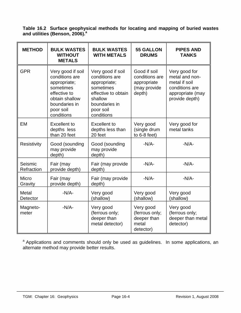
TGM: Chapter 16: Geophysics Page 16-4 Revision 1, August 2008
Table 16.2 Surface geophysical methods for locating and mapping of buried wastes and utilities (Benson, 2006).a
METHOD
BULK WASTES
WITHOUT METALS
BULK WASTES WITH METALS
55 GALLON DRUMS
PIPES AND
TANKS
GPR
Very good if soil conditions are appropriate; sometimes effective to obtain shallow boundaries in poor soil conditions
Very good if soil conditions are appropriate; sometimes effective to obtain shallow boundaries in poor soil conditions
Good if soil conditions are appropriate (may provide depth)
Very good for metal and non-metal if soil conditions are appropriate (may provide depth)
EM
Excellent to depths less than 20 feet
Excellent to depths less than 20 feet
Very good (single drum to 6-8 feet)
Very good for metal tanks
Resistivity
Good (sounding may provide depth)
Good (sounding may provide depth)
-N/A-
-N/A-
Seismic Refraction
Fair (may provide depth)
Fair (may provide depth)
-N/A-
-N/A-
Micro Gravity
Fair (may provide depth)
Fair (may provide depth)
-N/A-
-N/A-
Metal Detector
-N/A-
Very good (shallow)
Very good (shallow)
Very good (shallow)
Magneto-meter
-N/A-
Very good (ferrous only; deeper than metal detector)
Very good (ferrous only; deeper than metal detector)
Very good (ferrous only; deeper than metal detector)
a Applications and comments should only be used as guidelines. In some applications, an alternate method may provide better results.
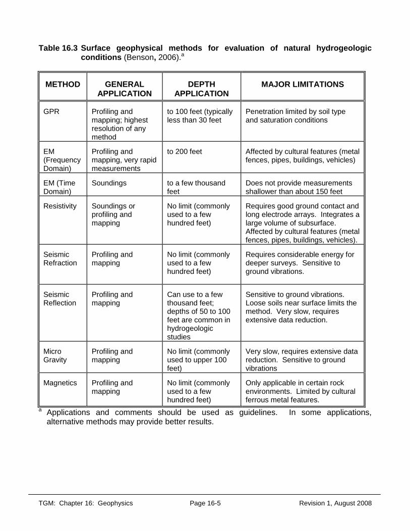
TGM: Chapter 16: Geophysics Page 16-5 Revision 1, August 2008
Table 16.3 Surface geophysical methods for evaluation of natural hydrogeologic conditions (Benson, 2006).a
METHOD
GENERAL
APPLICATION
DEPTH
APPLICATION
MAJOR LIMITATIONS
GPR
Profiling and mapping; highest resolution of any method
to 100 feet (typically less than 30 feet
Penetration limited by soil type and saturation conditions
EM (Frequency Domain)
Profiling and mapping, very rapid measurements
to 200 feet
Affected by cultural features (metal fences, pipes, buildings, vehicles)
EM (Time Domain)
Soundings
to a few thousand feet
Does not provide measurements shallower than about 150 feet
Resistivity
Soundings or profiling and mapping
No limit (commonly used to a few hundred feet)
Requires good ground contact and long electrode arrays. Integrates a large volume of subsurface. Affected by cultural features (metal fences, pipes, buildings, vehicles).
Seismic Refraction
Profiling and mapping
No limit (commonly used to a few hundred feet)
Requires considerable energy for deeper surveys. Sensitive to ground vibrations.
Seismic Reflection
Profiling and mapping
Can use to a few thousand feet; depths of 50 to 100 feet are common in hydrogeologic studies
Sensitive to ground vibrations. Loose soils near surface limits the method. Very slow, requires extensive data reduction.
Micro Gravity
Profiling and mapping
No limit (commonly used to upper 100 feet)
Very slow, requires extensive data reduction. Sensitive to ground vibrations
Magnetics
Profiling and mapping
No limit (commonly used to a few hundred feet)
Only applicable in certain rock environments. Limited by cultural ferrous metal features.
a Applications and comments should be used as guidelines. In some applications, alternative methods may provide better results.
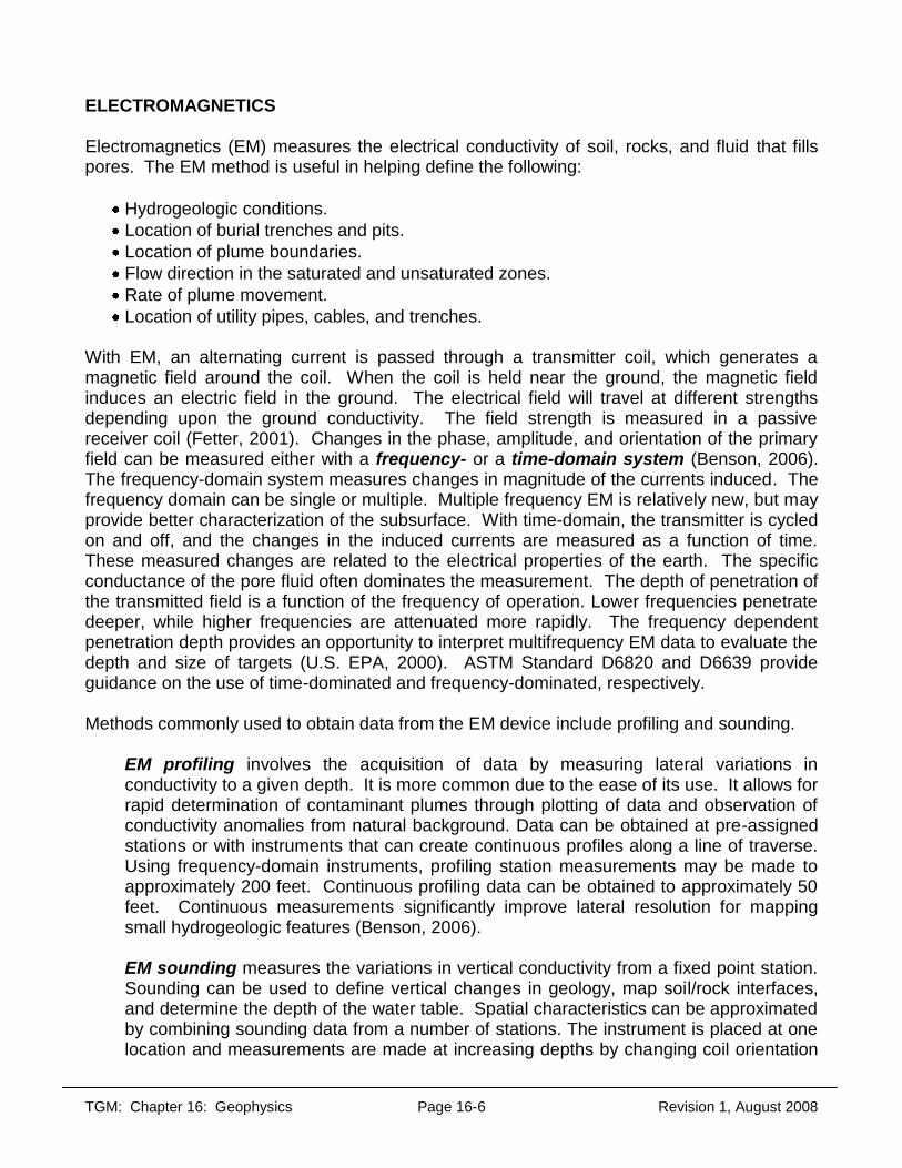
TGM: Chapter 16: Geophysics Page 16-6 Revision 1, August 2008
ELECTROMAGNETICS Electromagnetics (EM) measures the electrical conductivity of soil, rocks, and fluid that fills pores. The EM method is useful in helping define the following:
Hydrogeologic conditions. Location of burial trenches and pits. Location of plume boundaries. Flow direction in the saturated and unsaturated zones. Rate of plume movement. Location of utility pipes, cables, and trenches.
With EM, an alternating current is passed through a transmitter coil, which generates a magnetic field around the coil. When the coil is held near the ground, the magnetic field induces an electric field in the ground. The electrical field will travel at different strengths depending upon the ground conductivity. The field strength is measured in a passive receiver coil (Fetter, 2001). Changes in the phase, amplitude, and orientation of the primary field can be measured either with a frequency- or a time-domain system (Benson, 2006). The frequency-domain system measures changes in magnitude of the currents induced. The frequency domain can be single or multiple. Multiple frequency EM is relatively new, but may provide better characterization of the subsurface. With time-domain, the transmitter is cycled on and off, and the changes in the induced currents are measured as a function of time. These measured changes are related to the electrical properties of the earth. The specific conductance of the pore fluid often dominates the measurement. The depth of penetration of the transmitted field is a function of the frequency of operation. Lower frequencies penetrate deeper, while higher frequencies are attenuated more rapidly. The frequency dependent penetration depth provides an opportunity to interpret multifrequency EM data to evaluate the depth and size of targets (U.S. EPA, 2000). ASTM Standard D6820 and D6639 provide guidance on the use of time-dominated and frequency-dominated, respectively. Methods commonly used to obtain data from the EM device include profiling and sounding.
EM profiling involves the acquisition of data by measuring lateral variations in conductivity to a given depth. It is more common due to the ease of its use. It allows for rapid determination of contaminant plumes through plotting of data and observation of conductivity anomalies from natural background. Data can be obtained at pre-assigned stations or with instruments that can create continuous profiles along a line of traverse. Using frequency-domain instruments, profiling station measurements may be made to approximately 200 feet. Continuous profiling data can be obtained to approximately 50 feet. Continuous measurements significantly improve lateral resolution for mapping small hydrogeologic features (Benson, 2006). EM sounding measures the variations in vertical conductivity from a fixed point station. Sounding can be used to define vertical changes in geology, map soil/rock interfaces, and determine the depth of the water table. Spatial characteristics can be approximated by combining sounding data from a number of stations. The instrument is placed at one location and measurements are made at increasing depths by changing coil orientation

TGM: Chapter 16: Geophysics Page 16-7 Revision 1, August 2008
and/or spacing. Data can be acquired at depths ranging from 2.5 to 200 feet by using a variety of commonly available frequency-domain instruments. The vertical resolution of frequency-domain sounding is relatively poor because measurements are made at only a few depths. Time-domain transient systems are capable of providing detailed sounding data to depths of 150 to more than 1000 feet (Benson, 2006).
Soil and rock minerals, when dry, are characterized by low conductivities. On rare occasions, magnetite, graphite, and pyrite may occur in sufficient concentrations to increase natural conductivity significantly. Generally, conductivity is affected more by water content, porosity/permeability of the material, extent of pore space saturation, concentration of dissolved electrolytes and colloids, and the temperature and phase state (i.e., liquid, ice) of the pore water. Typical conductivity ranges have been determined for various soil and rock materials (Figure 16.1). Only ranges can be provided because conductivity can vary drastically within material types.
Inorganic contaminant plumes are mapped by noting increases (anomalies) in conductivity due to increases in free ions introduced by the contamination. This contribution of electrolytes/colloids to the ground water plume often increases conductivity values from one to three orders of magnitude over background. If non-polar, organic fluids are present (generally as free product), conductivity will decrease as soil moisture is displaced. As a result, organic free product plumes will map as anomalous decreases in conductivity. Organic plume delineation with EM is difficult and not commonly attempted. Typical EM noise or interference includes: power lines, atmospheric conditions, steel drums, fences, vehicles, railroad tracks, and buried utilities/pipes. These should be considered before any study is undertaken, and accounted for during data interpretation. DIRECT CURRENT (DC) RESISTIVITY The resistivity method involves the measurement of the ability of soil, rock and ground water to resist the flow of an electrical current. It is a function of the soil and rock matrix, percentage of fluid saturation and the conductivity of the pore fluids. Resistivity surveys are useful in providing supplemental information for:
Location and direction and rate of movement of contaminant plumes.
Location of burial sites (e.g., trenches, their depths and boundaries).
Hydrogeologic conditions (e.g., depth to water or water-bearing zones, depth to bedrock, thickness of soil, etc).
The method involves the injection of electrical current through a pair of surface electrodes inserted into the ground. A second pair is used to measure the resulting voltage. Several electrode configurations are used. The three most common arrays are Wenner, Schlumberger, and the dipole-dipole. These are described in Fetter (2001) and Sheriff (1989). Apparent resistivity is calculated based on the electrode separation, current applied, and measured voltage.
TGM: Chapter 16: Geophysics Page 16-8 Revision 1, August 2008
Figure 16.1 gives general ranges of resistivity in the natural environment. Soil and rock become less resistive (more conductive) as moisture/water content, porosity and permeability, dissolved solids, and colloid content increase. Clayey soils generally exhibit lower resistivity due to their high moisture and clay mineral content. Gravel has a higher resistivity than silt or clay under similar moisture conditions, as the electrically charged surfaces of finer particles are better conductors (Fetter, 2001). Contaminant plumes that display high total dissolved solids (TDS) concentrations cause lower resistivity measurements. Various problems can hinder the collection of accurate resistivity data. Dry surface material (high resistivity) can make injection of current very difficult. Roads and parking lots composed of asphalt and concrete may prevent electrode insertion and, therefore, limit the lateral extent of the survey. Common problems include:
Coupling between wires and reels.
Poor electrical contact with the ground.
Exceeding depth capabilities of instrument (power source and receiver sensitivity).
Cultural noise, including stray currents, potential fields and electromagnetic currents as a result of power lines, man-induced ground currents, fences, railroad tracks, and buried metallic pipes.
Heterogeneities in shallow conditions. It is not uncommon for a variety of geologic models to represent a single resistivity profile curve, and therefore, some preconception or data for subsurface geology is needed to verify the selected model. Resistivity surveys take more time than EM surveys, and space limitations also can hinder data collection. Success of the method is site-specific. In some cases, resistivity also outperforms EM and vice-versa. Like EM, profiling and sounding are the major methods for data acquisition. Resistivity sounding is used to determine vertical changes in the geologic section. Data is collected at fixed stations as the distance between electrodes is successively increased. As a consequence, the apparent resistivity is determined as a function of the effective depth of penetration. Apparent resistivity is an attempt to account for spatial in homogeneities and is a function of the electrode spacing. To interpret the data, the apparent resistivity values are plotted on log-log paper versus electrode spacing. The plots are compared to type curves or models to determine layer thicknesses, depths and true resistivities. These models are based on simple, uniformly layered ("layer cake") geologic conditions; therefore, they may oversimplify data interpretation for a more complex situation.

TGM: Chapter 16: Geophysics Page 16-9 Revision 1, August 2008
Figure 16.1 Range of electrical conductivities and resisitivities in natural soil and rock (Source: Benson et al., 1982.) Resistivity profiling involves moving an array of electrodes while keeping the array arrangement and spacing fixed (Sheriff, 1989). Lateral changes in resistivity are mapped, allowing for the delineation of contaminant plumes and of lateral changes in hydrogeologic conditions. For high resolution, stations should be spaced closely to increase accuracy. Electrode spacing can be varied to map lateral changes at varying depths, but this will slow the survey. Profiling can allow for rapid data interpretation by mapping apparent resistivity values and noting anomalous features relative to background. When mapping a plume, it is advantageous to conduct an initial sounding survey to determine plume depth and the appropriate electrode spacing, then continue with a profiling survey. Additional information on DC resistivity can be found in ASTM D6431-99 (2005).
Continuous resistivity profiling is a relatively new technique to assess the subsurface conditions under a water feature (e.g., river or lake). Contact USGS, Geophysical Technology Transfer Unit for additional information.
TGM: Chapter 16: Geophysics Page 16-10 Revision 1, August 2008
SPONTANEOUS POTENTIAL (SP) Spontaneous Potential measures natural voltage. It can be used as a surface or subsurface (borehole) technique. In surface techniques, non-polarizing probes containing a metal salt (copper sulfate) are used to connect the instrumentation to the surface of the earth. One electrode is fixed as the reference electrode, and the second roves. Lateral resolution is a function of station spacing.
The primary application of surface SP is assessing seepage from dams and embankments. Surface SP can also be used to investigate subsurface water movement and landslides, location of faults, drainage structures, shafts, tunnels and sinkholes, and coal mine fires. It is also possible that SP can be used to map geochemical variations associated with contaminant plumes. Depths of investigation are generally limited to 100 feet. Measurements are susceptible to interference from natural earth currents, soil conditions, topography, stray earth currents, cathodic protection currents, and cultural features. Corwin (1990) provides an overview of the method (ASTM D6429). SEISMIC METHODS Seismic methods are typically used to define natural geologic conditions, including top of bedrock; thickness, depth, composition, and physical properties of soil and rock; continuity of geologic strata; depth to water table, fracturing, faulting, and buried bedrock channels (Benson, 2006). Seismic methods have limited applications for determining buried wastes and cannot be used to locate contaminant plumes (see Tables 16.1- 16.3). Types of seismic methods include refraction and reflection. Additional information on seismic refraction and reflection can be found in ASTM standards D7128 and D6439, respectively. In addition, continuous seismic profiling is a relatively new technique to assess the subsurface conditions under a water feature (e.g., river or lake). Contact USGS, Geophysical Technology Transfer Unit for additional information. Seismic Refraction Refraction surveys, the predominant seismic method in hydrogeologic studies, measure seismic wave velocities of materials. A source (e.g., sledge hammer, gun device, weight, or explosives) is used to create and emit waves into the subsurface. These waves travel at material-specific velocities, are refracted at various interfaces, and eventually are received by surface geophones that convert them into an electrical signal that is displayed on a seismograph.
A variety of elastic waves result from the source and show up on the seismograph output. Typically, the compressional (primary or P) wave is the only wave of concern. This wave travels fastest and is the first to arrive at the geophones, making its determination relatively easy. Physical properties determine the velocity at which the primary wave will travel through a particular geologic material or layer. For example, porosity, mineral composition, and water content affect material density and elasticity, which in turn affect velocity. Benson et al. (1982) provided common velocity ranges for various materials. Overlap between materials
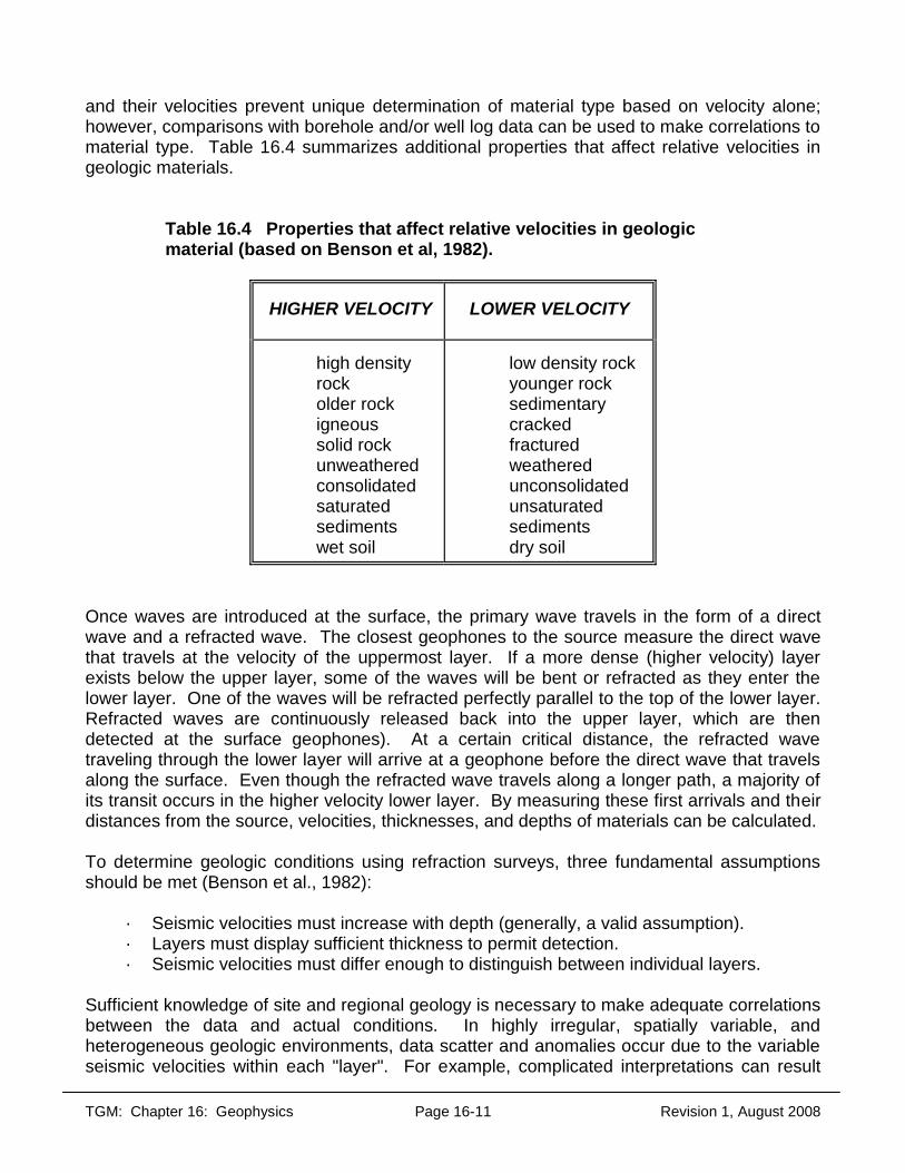
TGM: Chapter 16: Geophysics Page 16-11 Revision 1, August 2008
and their velocities prevent unique determination of material type based on velocity alone; however, comparisons with borehole and/or well log data can be used to make correlations to material type. Table 16.4 summarizes additional properties that affect relative velocities in geologic materials.
Table 16.4 Properties that affect relative velocities in geologic material (based on Benson et al, 1982).
HIGHER VELOCITY
LOWER VELOCITY
high density rock older rock igneous solid rock unweathered consolidated saturated sediments wet soil
low density rock younger rock sedimentary cracked fractured weathered unconsolidated unsaturated sediments dry soil
Once waves are introduced at the surface, the primary wave travels in the form of a direct wave and a refracted wave. The closest geophones to the source measure the direct wave that travels at the velocity of the uppermost layer. If a more dense (higher velocity) layer exists below the upper layer, some of the waves will be bent or refracted as they enter the lower layer. One of the waves will be refracted perfectly parallel to the top of the lower layer. Refracted waves are continuously released back into the upper layer, which are then detected at the surface geophones). At a certain critical distance, the refracted wave traveling through the lower layer will arrive at a geophone before the direct wave that travels along the surface. Even though the refracted wave travels along a longer path, a majority of its transit occurs in the higher velocity lower layer. By measuring these first arrivals and their distances from the source, velocities, thicknesses, and depths of materials can be calculated. To determine geologic conditions using refraction surveys, three fundamental assumptions should be met (Benson et al., 1982):
· Seismic velocities must increase with depth (generally, a valid assumption). · Layers must display sufficient thickness to permit detection. · Seismic velocities must differ enough to distinguish between individual layers.
Sufficient knowledge of site and regional geology is necessary to make adequate correlations between the data and actual conditions. In highly irregular, spatially variable, and heterogeneous geologic environments, data scatter and anomalies occur due to the variable seismic velocities within each "layer". For example, complicated interpretations can result

TGM: Chapter 16: Geophysics Page 16-12 Revision 1, August 2008
when investigating poorly sorted glacial tills, perched water table conditions, bedrock formations with cementation differences, irregular bedrock surfaces, and highly dissolved limestone formations. Simple, uniform geology allows for easier interpretation and more accurate results. Refraction surveys are often used to determine the depth of the water table, although the feasibility depends on site conditions. The water table can be readily identified in coarse-grained sand and gravel, where a distinct boundary between the saturated and unsaturated zones exists. In fine-grained sands, silts and clays, where natural capillary forces cause a very irregular and poorly defined saturated/unsaturated boundary, determination is difficult. The depth of penetration is based on the length and spacing of the entire geophone line. Length in general should be 3 to 5 times the maximum depth of interest (Benson et al., 1982). Spacings of 5 to 50 feet are common for adequate resolution, but closer spacing may be necessary for higher resolution in shallow materials. Also, a greater energy source is needed as the desired depth of penetration increases. A sledge hammer can be utilized to reach depths of 30 to 50 feet (Benson et al., 1982). A drop weight or other mechanical impactors are sometimes used to reach depths from 150 to 350 feet. Special explosives may be necessary if greater depths are necessary. Because refraction surveys measure ground vibrations, the method is very sensitive to background noise (moving vehicles, strong winds blowing through trees, field crew movement, etc.). Interference can be overcome by signal enhancement, which involves repeated hammer blows at the same station to build the true seismic signal above and beyond the signals produced by the noise. Seismic Reflection Seismic reflection surveys involve measuring the wave reflected back to the surface. By comparison, deeper investigations can be conducted with less energy than can the refraction method. The reflection method can provide information at depths less than 10 feet; however, it is more typically applied at 50 to 100 feet. The method can provide relatively detailed geological sections to a few thousand feet (Benson, 2006). Seismic frequencies used for shallow studies should be relatively high (150 and 600 Hz) to improve vertical resolution. The ability to collect high frequency information may be limited by site conditions. Loose soil near the surface makes it difficult for the soil system to transmit high frequency energy. Because of the need for higher frequencies, attention must be given to selection of a source and its optimum coupling to soil or rock, as well as the geophone spacing. In general, the same source used for the refraction method can be applied to the reflection method. The geophones should be closely spaced (1 to 20 feet) to provide good lateral resolution. The most common limitation of seismic reflection is acoustic noise from natural or cultural sources (Benson, 2006). Additional information on seismic reflection can be found in ASTM D7128-05.

TGM: Chapter 16: Geophysics Page 16-13 Revision 1, August 2008
METAL DETECTION Metal detectors can locate any kind of metallic material, including ferrous (iron, steel) and non-ferrous (aluminum, copper). The tool is useful for locating shallow buried drums, trenches containing drums, underground storage tanks and metallic piping. It also can play an important safety role by locating utility pipes and cables prior to drilling or digging.). Additional information on magnetic surveys can be found in ASTM D7046-04. Types of metal detection devices include pipeline/cable locators, conventional "treasure hunter" detectors, and specialized detectors. Conventional detectors utilize small coils for detection of coin-sized objects. This limits their use to very shallow depths. Specialized detectors are designed to handle unique, site-specific problems. They are typically designed to enhance detection depths, increase area coverage, and continuously record data. They are expensive and require additional expertise to operate. A metal detector responds to the electrical conductivity of objects. Metal objects typically display much higher conductivities than soil. Transmitting coils create a magnetic field that is in balance with the receiving coil. When metal comes in contact with the induced magnetic field emitted from the transmitting coil, a secondary field develops. This results in an imbalance between the transmitting and receiving coils. The instrument then indicates that a metallic object has been encountered (Benson et al., 1982). Metal detector response is directly related to size and depth of the buried object. The larger the surface area of the object, the greater the depth of detection will be. Small metal objects, like quart-sized containers, can be detected at 2 to 3 feet (Benson et al., 1982). Larger objects, like 55 gallon drums, are typically detected at 3 to 10 feet. Piles of drums can be detected at 10 to 20 feet. Metal detector response is inversely proportional to the sixth power of the depth of the target (1/depth6). Therefore, if the depth of the target is doubled, the response will decrease by a factor of 64. Most objects, no matter how large, fall out of the range of metal detectors at depths greater than 20 feet (Benson et al., 1982). Coil response also affects metal detector response. Smaller diameter coils will limit detection depths, but enhance small object sensitivity. Large diameter coils will enhance detection depth, but decrease small object sensitivity. Metal detection is extremely sensitive to noise. Any surface metallic objects can affect the instrument. Locations of fences, buildings, buried pipes, and metal objects should be identified. Furthermore, high concentrations of natural iron minerals in the soil can indicate a false target. Additionally, high concentrations of salt water, acids, and other conductive fluids can create detection problems. Many of these problems can be reduced when the transmitting and receiving coils are nulled or balanced before the survey begins. As a result, all background noise will be filtered. MAGNETOMETRY A magnetometer is used to measure the intensity of the earth's magnetic field. This instrument is typically used to locate ferrous objects, boundaries of trenches buried with ferrous containers, and underground utilities (pipes and tanks) and the permeable pathways associated with them (Benson et al., 1982) (see Tables 16.1-16.3).

TGM: Chapter 16: Geophysics Page 16-14 Revision 1, August 2008
A natural magnetic field exists in and around the earth's surface. The intensity of this field varies considerably. In the U.S., it is typically around 50,000 gammas. The presence or absence of ferrous metals alters the intensity of the magnetic field. If natural magnetic properties are uniform, buried metallic objects display a local anomaly that is detected (Benson et al., 1982). Piles of buried drums can yield anomalies of 100 to 1000 gammas. The magnetometer is susceptible to a variety of cultural noise, which includes metal buildings and fences, overhead power lines, and buried utilities.
Total field and gradient are the two common types of magnetic measurements (Benson, 2006). Total field measurement responds to the total magnetic field of the earth, natural and cultural magnetics, and any changes caused by a target. However, measurement of such a large scale field can inhibit device effectiveness. This problem can be reduced by establishing a base station magnetometer to obtain background data and subtracting the values from measurements. This reduces the effects of natural noise and long-term changes of the earth's magnetic field, but does not reduce the effects of cultural noise (Benson, 2006). Total field magnetometer response is directly proportional to the mass of the ferrous object or target and inversely proportional to the cube of the distance to the target. A single drum can be detected up to 20 feet in depth and a massive pile of drums to 50 feet with a total field magnetometer (Benson, 2006). If anomalies of interest are expected to be of similar magnitude to natural field variations, it is necessary to assess the site-specific noise and instrument repeatability by taking at least two readings at each station. Repeated measurements should agree within 1 gamma. Values that do not repeat within 10 gammas should not be used. Values that repeat between 1 and 10 gammas should be averaged. Gradient measurements using a gradiometer also can be used to alleviate problems. This device is basically two magnetometers separated vertically (or horizontally) by a few feet. Gradient can also be obtained by taking two total field readings at different heights above the ground. Gradient measurements are insensitive to natural spatial and temporal changes in the earth's magnetic field and experience minimal effects from cultural features. A gradiometer only measures the difference between two total fields and, therefore, only responds to the local magnetic gradient (Benson, 2006). A gradiometer's response is inversely proportional to the fourth power of the distance to the target. Therefore, the device is less sensitive than a total field magnetometer. A gradiometer is better able to locate small targets, such as a barrel, and can detect a single drum up to depths of 10 feet, and massive piles of drums up to 25 feet (Benson, 2006). GRAVIMETRY Gravity instruments measure minute changes in the earth's gravity due to changes in density of subsurface materials. The gravity method is useful in delineating buried valleys, bedrock topography, and geologic structural voids, and locating bulk buried waste. Due to the extensive time and effort required to acquire the data and then reduce it, gravity studies are not typically applied to site-specific investigations.

TGM: Chapter 16: Geophysics Page 16-15 Revision 1, August 2008
Benson (2006) refers to two types of surveys: regional and local. Regional surveys involve the collection of measurements over a large area with widely spaced stations (thousands of feet to miles) to determine large scale, regional features, often at great depth. Local surveys involve the acquisition of measurements in small areas with station spacings of 5 to 20 feet to locate shallow features such as buried valleys and fractures. Gravimeters have been designed to measure in milligals, the unit measure of acceleration of gravity1. The instruments have been designed with thermostats to prevent drift due to changes in temperature. Ground noise, wind, and earth tides also may affect the measurements. About every hour, the instrument should be returned to an assigned base station and a measurement taken to record any drift that may be occurring. Corrections can then be applied to the data. The instrument should be handled carefully to prevent sudden jarring.
The data recorded in the field requires extensive reduction before any interpretations can be made. It should be corrected for earth tides, changes in elevation (all stations must be surveyed to 0.01 feet), latitude, and topography. This data can then be plotted as a gravity profile, from which interpretations are made. Careful interpretation is necessary because a variety of geologic situations can be represented by a single profile.
DOWNHOLE GEOPHYSICAL METHODS Geophysical techniques provide an efficient and cost-effective means to obtain vertical profiles of a measured parameter within a borehole or well. Techniques for ground water investigations have been adapted from long-standing practices in the oil industry. A variety of methods have been developed to determine subsurface lithology and physical properties (such as porosity, density, seismic velocity, and elastic moduli) and identify permeable or fluid-bearing zones. These methods or "logs" provide continuous measurements of properties along the entire length of a borehole. By comparing data for a borehole for which geology is unknown to data for a borehole for which a complete, detailed knowledge of geology is available, the geology of the unknown borehole can be determined. The geophysical logging system consists of probes, cable and drawworks, power and processing modules, and data recording units (figure 16.2). State-of-the-art logging systems are controlled by a computer and can collect multiple logs with one pass of the probe. Each technique has specific requirements and limitations that must be considered. For example, most logs provide measurements within a radius of 6 to 12 inches from the instrument (Benson, 2006). As the well diameter increases, instrument response may be greatly affected by the drilling method and components of well completion. Nuclear logs can be conducted in an open borehole as well as through steel or PVC well casing. Some techniques can only be conducted in open boreholes, which may limit their use in loosely consolidated, slumping materials where open conditions cannot be maintained. Certain instruments can only perform under saturated conditions, further limiting application. The presence of drilling muds and smearing of fine particles during drilling can affect instrument
1The earth' s normal gravity is 980 gals.

TGM: Chapter 16: Geophysics Page 16-16 Revision 1, August 2008
response and result in inaccurate interpretations. Table 16.5 summarizes the characteristics and use of commonly utilized downhole logging instruments, while Table 16.6 summarizes the common applications. ASTM D5753-05 provides additional references and general guidance on planning and conducting borehole geophysical logging. Information in the standard includes: general logging procedures, documentation, calibration, and factors that can affect the quality of logging.
Figure 16.2. Geophysical logging (http://ny.water.usgs.gov/projects/bgag/schematic.html) USGS Web site http://water.usgs.gov/ogw/bgas/methods.html NUCLEAR LOGS Nuclear logging tools are used to evaluate stratigraphy, ground water conditions, and subsurface contaminant distribution. Types include: (1) tools that measure the natural radioactivity of a formation, and (2) tools that emit radiation and measure the corresponding response of the formation. The first type measures gamma radiation emissions from naturally occurring uranium, thorium, and radioactive potassium present within clay minerals, and it is useful in distinguishing clay-rich strata from sand-rich strata. The second type exposes the
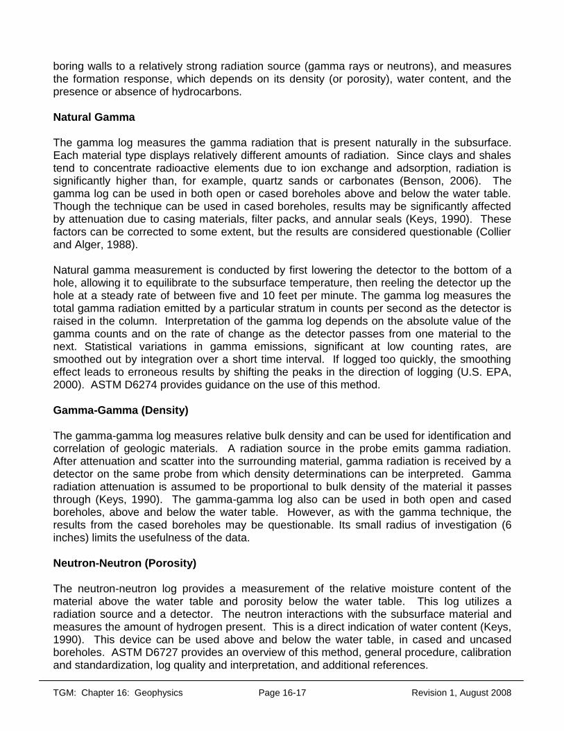
TGM: Chapter 16: Geophysics Page 16-17 Revision 1, August 2008
boring walls to a relatively strong radiation source (gamma rays or neutrons), and measures the formation response, which depends on its density (or porosity), water content, and the presence or absence of hydrocarbons. Natural Gamma The gamma log measures the gamma radiation that is present naturally in the subsurface. Each material type displays relatively different amounts of radiation. Since clays and shales tend to concentrate radioactive elements due to ion exchange and adsorption, radiation is significantly higher than, for example, quartz sands or carbonates (Benson, 2006). The gamma log can be used in both open or cased boreholes above and below the water table. Though the technique can be used in cased boreholes, results may be significantly affected by attenuation due to casing materials, filter packs, and annular seals (Keys, 1990). These factors can be corrected to some extent, but the results are considered questionable (Collier and Alger, 1988). Natural gamma measurement is conducted by first lowering the detector to the bottom of a hole, allowing it to equilibrate to the subsurface temperature, then reeling the detector up the hole at a steady rate of between five and 10 feet per minute. The gamma log measures the total gamma radiation emitted by a particular stratum in counts per second as the detector is raised in the column. Interpretation of the gamma log depends on the absolute value of the gamma counts and on the rate of change as the detector passes from one material to the next. Statistical variations in gamma emissions, significant at low counting rates, are smoothed out by integration over a short time interval. If logged too quickly, the smoothing effect leads to erroneous results by shifting the peaks in the direction of logging (U.S. EPA, 2000). ASTM D6274 provides guidance on the use of this method. Gamma-Gamma (Density) The gamma-gamma log measures relative bulk density and can be used for identification and correlation of geologic materials. A radiation source in the probe emits gamma radiation. After attenuation and scatter into the surrounding material, gamma radiation is received by a detector on the same probe from which density determinations can be interpreted. Gamma radiation attenuation is assumed to be proportional to bulk density of the material it passes through (Keys, 1990). The gamma-gamma log also can be used in both open and cased boreholes, above and below the water table. However, as with the gamma technique, the results from the cased boreholes may be questionable. Its small radius of investigation (6 inches) limits the usefulness of the data. Neutron-Neutron (Porosity) The neutron-neutron log provides a measurement of the relative moisture content of the material above the water table and porosity below the water table. This log utilizes a radiation source and a detector. The neutron interactions with the subsurface material and measures the amount of hydrogen present. This is a direct indication of water content (Keys, 1990). This device can be used above and below the water table, in cased and uncased boreholes. ASTM D6727 provides an overview of this method, general procedure, calibration and standardization, log quality and interpretation, and additional references.
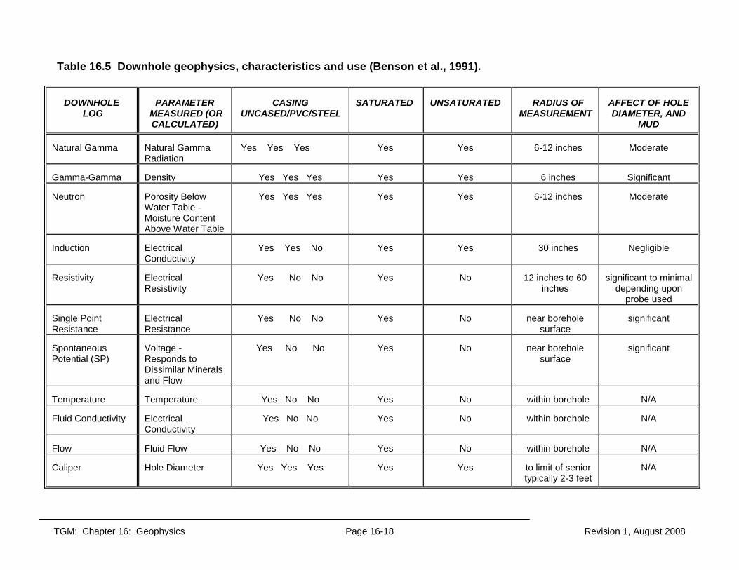
TGM: Chapter 16: Geophysics Page 16-18 Revision 1, August 2008
Table 16.5 Downhole geophysics, characteristics and use (Benson et al., 1991). DOWNHOLE LOG
PARAMETER MEASURED (OR CALCULATED)
CASING UNCASED/PVC/STEEL
SATURATED
UNSATURATED
RADIUS OF MEASUREMENT
AFFECT OF HOLE DIAMETER, AND MUD
Natural Gamma
Natural Gamma Radiation
Yes Yes Yes
Yes
Yes
6-12 inches
Moderate
Gamma-Gamma
Density
Yes Yes Yes
Yes
Yes
6 inches
Significant
Neutron
Porosity Below Water Table - Moisture Content Above Water Table
Yes Yes Yes
Yes
Yes
6-12 inches
Moderate
Induction
Electrical Conductivity
Yes Yes No
Yes
Yes
30 inches
Negligible
Resistivity
Electrical Resistivity
Yes No No
Yes
No
12 inches to 60
inches
significant to minimal
depending upon probe used
Single Point Resistance
Electrical Resistance
Yes No No
Yes
No
near borehole
surface
significant
Spontaneous Potential (SP)
Voltage - Responds to Dissimilar Minerals and Flow
Yes No No
Yes
No
near borehole
surface
significant
Temperature
Temperature
Yes No No
Yes
No
within borehole
N/A
Fluid Conductivity
Electrical Conductivity
Yes No No
Yes
No
within borehole
N/A
Flow
Fluid Flow
Yes No No
Yes
No
within borehole
N/A
Caliper
Hole Diameter
Yes Yes Yes
Yes
Yes
to limit of senior typically 2-3 feet
N/A

TGM: Chapter 16: Geophysics Page 16-19 Revision 1, August 2008
Table 16.6 Summary of log application (Keys and MacCary, 1971).
REQUIRED INFORMATION ON THE PROPERTIES OF ROCKS, FLUID, WELLS,
OR THE GROUND WATER SYSTEM
WIDELY AVAILABLE LOGGING TECHNIQUES THAT MIGHT BE UTILIZED
Lithology and stratigraphic correlation of aquifers and associated rocks
Electric, sonic, or caliper logs made in open holes; nuclear logs made in open or cased holes
Total porosity or bulk density
Calibrated sonic logs in open holes, calibrated neutron or gamma-gamma logs in open or cased holes
Effective porosity or true resistivity
Calibrated log-normal resistivity logs
Clay or shale content
Gamma logs
Permeability
No direct measurement by logging. May be related to porosity, injectivity, sonic amplitude, and fractures
Secondary permeability-fractures, solution openings
Caliper, sonic, or borehole televiewer or television logs
Specific yield of unconfined aquifers
Calibrated neutron logs
Grain size Possible relation to formation factor derived from electric logs
Location of water level or saturated zones
Electric, temperature, or fluid conductivity in open hole or inside casing, neutron or gamma-gamma logs in open hole or outside casing
Moisture content
Calibrated neutron logs
Infiltration
Time interval neutron logs under special circumstances or radioactive tracers
Direction, velocity, and path of ground water flow
Single-well tracer techniques-point dilution and single-well pulse; multiwell tracer techniques
Dispersion, dilution, and movement of waste
Fluid conductivity and temperature logs, gamma logs for some radioactive wastes, fluid sampler
Source and movement of water in a well
Injectivity profile; flowmeter or tracer logging during pumping or injection; temperature logs
Chemical and physical characteristics of water, including salinity, temperature, density, and viscosity
Calibrated fluid conductivity and temperature in the well; neutron chloride logging outside casing; multi-electrode resistivity
Determining construction of existing wells, diameter and position of casing, perforations, screen
Gamma-gamma, caliper, collar, and perforation locator; borehole television
Guide to screen setting
All logs providing data on the lithology, water-bearing characteristics, and correlation and thickness of aquifers
Cementing Caliper, temperature, gamma-gamma; acoustic for cement bond
Casing corrosion
Under some conditions, caliper or collar locator
Casing leaks and (or) plugged screen
Tracer and flowmeter

TGM: Chapter 16: Geophysics Page 16-20 Revision 1, August 2008
NON-NUCLEAR OR ELECTRIC LOGGING Non-nuclear or electric logging encompasses logs in which a record of potential differences in electric current is measured. For the systems to provide useful data, the pore fluid must be conductive. This may not always be the case. Electric logging tools commonly used include induction, resistivity, single-point resistance, spontaneous potential, and acoustic. Induction The induction log measures the electrical conductivity of the subsurface material. Conductivity variations result from changes in porosity, permeability, rock type, and fluid content. Changes in materials due to variations in conductivity can be identified. This log can be utilized without direct electrical contact with the formation, which allows for its use in both saturated and unsaturated conditions. It also can penetrate PVC well casing (Benson, 2006). Specific conductance of the pore fluid has a major influence on instrument response. Therefore, the induction log can be used to identify inorganic contaminant plumes or organic plumes containing inorganic constituents. ASTM D6726 provides a more detailed overview of this method, general procedure, calibration and standardization, log quality and interpretation, and additional references. Resistivity The resistivity log provides measurements of the apparent resistivity of the material surrounding a borehole (Benson, 2006). Resistivity is the reciprocal of conductivity and, therefore, this log measures the same properties and has the same applications as the induction log. Direct electrical contact is needed. Therefore, the technique can only be used in uncased boreholes in saturated materials. ASTM D6726 provides a more detailed overview of this method, general procedure, calibration and standardization, log quality and interpretation, and additional references. Single-Point Resistance The single-point resistance log provides a record of the resistance between surface and downhole electrodes of the instrument. Resistance logs are used primarily for lithologic determination, correlation, and identification of fractures and washout zones (Benson, 2006). Single-point logs do not provide a quantitative measure of resistance for the surrounding material. The resistance log is limited to use in uncased boreholes in saturated materials. Spontaneous-Potential The spontaneous-potential log (SP) is a record of the natural potential or voltage that develops between the borehole fluid and the surrounding materials. Spontaneous-potential is a function of fluid chemical activities, temperature, and the type and quantity of clay present, and is not related to porosity and permeability (Keys, 1990). Electrochemical and electrokinetic or streaming potentials, caused by water moving through permeable material, are the primary sources of spontaneous-potential. Oxidation-reduction potential is another source (Keys, 1990). Measurements are subject to considerable noise from the electrodes, hydrogeologic conditions, and borehole fluid (Benson, 2006). Though quantitative results are

TGM: Chapter 16: Geophysics Page 16-21 Revision 1, August 2008
not provided, the SP may be useful in determining lithology, oxidation-reduction conditions, and fluid flow (Benson, 2006). The SP is limited to use in uncased boreholes under saturated conditions. Acoustic Acoustic logging includes techniques that use a transducer to transmit a sonic wave through the fluids in a borehole and the surrounding rock. The techniques can provide information on porosity, lithology, cement, and the location and character of fractures. Types described by Keys (1990) include velocity, wave, cement bond, and teleview. All require fluid in the borehole to couple the signal to the surrounding rock. They differ in the frequencies used, the way the signal is recorded, and the purpose of use. Velocity logs can be used to help identify lithology and measure porosity. These logs are generally limited in use to consolidated deposits and uncased, fluid-filled boreholes. Cement bond logs provide information on the quality of the bond between the borehole and cement and the casing and cement. Wave form logs have not been extensively used in hydrogeologic studies; however, they are needed to accurately interpret cement bond logs. A televiewer is a logging device that can provide high-resolution information on the location and characterization of secondary porosity (e.g., fractures and solution channels). The technique can also provide information on the strike and dip of planar features. PHYSICAL LOGS Physical methods include temperature, conductivity and caliper logging. Use of these logs often is necessary to properly interpret other geophysical logs. Temperature The temperature log provides a continuous recording for any fluid that a sensor probe contacts. It can provide information on movement of water through a borehole, trace movement of injected waste or water, and correct other logs sensitive to temperature. Types of logs that are common are temperature and differential temperature. The differential log is a record of the rate of change per depth (Keys, 1990). Fluid Conductivity Fluid conductivity logs provide data related to dissolved solids concentration in the fluid column. Conductivity is sensitive to temperature. If accurate conductivity values are needed, a temperature log record should also be taken to correct the data. Although the quality of the fluid in the borehole column may not reflect the quality of the adjacent interstitial fluids, the information may be useful when combined with other logs (Keys, 1990). Fluid Flow Flow measurements with logging probes can be performed by mechanical, tracer and thermal methods. The most common flow logging probe used is an impeller-type device.

TGM: Chapter 16: Geophysics Page 16-22 Revision 1, August 2008
Caliper The caliper log provides a measure of the diameter of the cased or uncased borehole. This log is essential in interpreting other logs that are affected by changes in borehole diameter (Keys, 1990). It also can provide information for locating slumping or cavities and fractures in the open borehole walls. In cased wells, the caliper log can be useful for determining construction details and may reveal accumulation of minerals or corrosion of the casing itself (Benson, 2006).
DOCUMENTATION
If surface or downhole geophysical methods are utilized, it is important that the entire process be documented. Some of the features that should be presented are:
Objective of the study, including description of the targets of interest.
Description of chosen technique(s) and the rationale for their selection.
Description of site location and the cultural and geologic/hydrogeologic setting (regional and site-specific, if available).
Description of survey set-up, instrumentation, calibration, and data collection.
Procedures for quality assurance and quality control.
Summary of the collected data (including raw and corrected). Raw data and data files
used for computer modeling should be kept on file and made available, if requested.
Summary of data reduction.
Interpretation of the data, including any correlations made from existing data.
Site map.
Any maps, graphs, traverses, profiles associates with the geophysical method. These should be labeled and contain details appropriate to the particular geophysical technique.
Documentation of all problems encountered, and steps taken, if any, to solve them.

TGM: Chapter 16: Geophysics Page 16-23 Revision 1, August 2008
REFERENCES
ASTM D5753-05. Standard Guide for Planning and Conducting Borehole Geophysical Logging. American Society of Testing Material Standards. West Conshohocken, Pennsylvania.
ASTM D5777-00(2006). Standard Guide for Using Seismic Refraction Method for
Subsurface Investigation. American Society of Testing Material Standards. West Conshohocken, Pennsylvania
ASTM D6274ASTM-98(2004) Standard Guide for Conducting Borehole Geophysical
Logging-Gamma American Society of Testing Material Standards. West Conshohocken, Pennsylvania
ASTM D6429-99(2006). Standard Guide for Selecting Surface Geophysical Methods.
American Society of Testing Material Standards. West Conshohocken, Pennsylvania ASTM D6639-01 Standard Guide for Using the Frequency Domain Electromagnetic Method
for Subsurface Investigations. American Society of Testing Material Standards. West Conshohocken, Pennsylvania
ASTM D6431-99(2005). Standard Guide for Using the Direct Current Resistivity Method for
Subsurface Investigation. American Society of Testing Material Standards. West Conshohocken, Pennsylvania.
ASTM D6432 99(2005). Standard Guide for Using the Surface Ground Penetrating Radar for
Subsurface Investigation. American Society of Testing Material Standards. West Conshohocken, Pennsylvania.
ASTM D6639-01 Standard Guide for Using the Frequency Domain Electromagnetic Method
for Subsurface Investigations. American Society of Testing Material Standards. West Conshohocken, Pennsylvania.
ASTM D6726-01(2007). Standard Guide for Conducting Borehole Geophysical Logging-
Electromagnetic Induction. American Society of Testing Material Standards. West Conshohocken, Pennsylvania
ASTM D6727-01(2007). Standard Guide for Conducting Borehole Geophysical Logging-
Neutron. American Society of Testing Material Standards. West Conshohocken, Pennsylvania
ASTM D6820-02(2007). Standard Guide for Use of Time Domain Electromagnetic Method
for Subsurface Investigation. American Society of Testing Material Standards. West Conshohocken, Pennsylvania
ASTM D7046-04. Standard Guide for Use of Metal Detection Method for Subsurface Investigation. American Society of Testing Material Standards. West Conshohocken, Pennsylvania
TGM: Chapter 16: Geophysics Page 16-24 Revision 1, August 2008
ASTM D7128-05. Standard Guide for Using Sesmic-Reflection Method for Subsurface Investigation. American Society of Testing Material Standards. West Conshohocken, Pennsylvania
ASTM D7400-07. Standard Test Method for Downhole Seismic Testing. American Society
of Testing Material Standards. West Conshohocken, Pennsylvania Benson, R. C., R. A. Glaccum, and M. R. Noel. 1982. Geophysical Techniques for Sensing
Buried Wastes and Waste Migration. Environmental Monitoring Systems Laboratory,Office of Research and Development. U.S. Environmental Protection Agency. Las Vegas, Nevada.
Benson, R.C. 2006. Remote Sensing and Geophysical Methods for Evaluation of Subsurface
Conditions. In: David M. Nielsen (editor), Practical Handbook of Ground Water Monitoring. Lewis Publishers, Inc. Chelsea, Michigan. pp.249-296.
Collier, H.A. and Alger, R.P. 1988. Recommendations for Obtaining Valid Data From
Borehole Geophysical Logs. Proceedings From the Second National Outdoor Action Conference on Aquifer Restoration, Ground Water Monitoring and Geophysical Methods. National Water Well Association. Dublin, Ohio pp. 897-923.
Corwin, R.F. 1990. The Self-Potential Method for Environmental and Engineering
Applications. Geotechnical and Environmental Geophysics. Volume I: Review and Tutorial. S.H. Ward (ed.). Society of Exploration Geophysics.
Fetter, C. W. 2001. Applied Hydrogeology. Third Edition. Macmillan College Publishing
Company. New York, New York. Keys, W. S. and L. M. MacCary. 1971. Techniques of Water Resources Investigation of the
United States Geological Survey, Chapter E1: Application of Borehole Geophysics to Ground Water Investigations. U.S. Geologic Survey. Book 2: Collection of Environmental Data. U.S. Government Printing Office. Washington, D.C.
Keys, W. S. 1990. Borehole Geophysics Applied to Ground-Water Investigations. U.S.
Geological Survey Techniques of Water Resources Investigations. Book 2, Chapter E2. United States Government Printing Office. Denver, Colorado.
Sheriff, R.E. 1989. Geophysical Methods. Prentice Hall. Englewood Cliffs, New Jersey. U.S. EPA 2001. Innovations in Site Characterization: Geophysical Investigations at
Hazardous Waste Sites. Office of Solid Waste and Emergency Response. Unites States Environmental Protection Agency. EPA 542-R-00-003.
U.S. EPA. 1997. Chapter III: Surface Geophysical Methods. In: Expedited Site Assessment
Tools for Underground Storage Tanks: A Guide for Regulators. EPA 510-B-970001. Office of Underground Storage Tanks. United States Environmental Protection Agency.

TGM: Assessment of Aquitard Page 1-9 Revision 0, November, 2009
TITLE: Assessment of an Aquitard during a Ground Water Contamination
Investigation DATE: November, 2009. SUBJECT: Guidance for evaluating whether an aquitard adequately protects underlying ground water when an overlying ground water zone is contaminated. BACKGROUND: When investigating contaminated ground water, aquitards typically need to be evaluated. Aquitards are low hydraulic conductivity geologic deposits that help protect ground water resources from contamination by impeding downward flow. Aquitards can decrease the susceptibility of underlying ground water to contamination by increasing both time of travel and the flow path distance from contaminated overlying ground water sources. However, no geologic formation or stratum is completely impermeable; some ground water flows across even the least permeable aquitards, given sufficient time. An assessment of the degree to which an aquitard can restrict the movement of ground water and contaminants is critical when evaluating the susceptibility of ground water underlying an aquitard. Situations where evaluation of an aquitard may be needed include, but are not limited to:
Evaluating areas of known or suspected soil and ground water contamination Siting new drinking water wells Designing a monitoring well network Designing or planning a ground water remediation system
GUIDANCE: This guidance is designed for users who may need to monitor and/or investigate ground water zones beneath a contaminated ground water zone. It is designed for a reader who has an understanding of hydrogeology and contaminant transport. There is no “cookbook” or “one size fits all” approach for determining whether an aquitard provides adequate protection. The user should collect pertinent data and make a “weight-of-evidence” decision. When evaluating the protective capabilities of an aquitard, the hydrogeologic characteristics and the contaminant characteristics should be considered. In general, some or all of the information listed below should be evaluated. Regardless of the conclusion regarding an aquitard’s protectiveness, ground water sampling from underlying ground water zones may be required. The user should contact the Ohio EPA division having regulatory authority. 1. Material type and hydraulic conductivity. The degree to which an aquitard
protects underlying ground water resources depends on the vertical hydraulic conductivity, which is largely controlled by the type of material. The classification of

TGM: Assessment of Aquitard Page 2-9 Revision 0, November, 2009
the material composing the aquitard (e.g., shales, clays, silty clays) can be determined by visual observation of geologic borings samples, tests pits, trenches or through laboratory analyses of soil or rock samples. Vertical hydraulic conductivity (Kv) is generally determined by laboratory analysis of undisturbed samples (i.e., Shelby tube) or by in-situ techniques, such pumping tests. Horizontal hydraulic conductivity may affect the Kv in an aquitard as it may influence the transport of water to fractures. The number of borings and laboratory samples needed depends on the geologic heterogeneity of the aquitard. In general, clays and silty clays with low vertical hydraulic conductivity (e.g., >1× 10-07 cm/sec) will more effectively protect underlying ground water than sands and gravels (Kv ≥× 10-04 cm/sec). Competent shale or some other relatively impermeable bedrock may also effectively isolate underlying ground water.
2. Thickness. The aquitard thickness is generally determined from geologic borings.
Geophysical techniques, such as seismic refraction, resistivity, and borehole gamma-ray logs, also may be useful. In general, aquitards that are tens of feet thick protect better than thinner, low-permeability zones.
A 30-feet thick clay zone is often considered sufficient to protect underlying ground water. However, evaluating the degree of protection should not be based solely on thickness. Other criteria, such as material type, vertical and lateral discontinuities, presence/absence of hydraulically active fractures, and contaminant characteristics and concentrations should also be considered.
3. Lateral continuity. Aquitards that are laterally continuous generally provide better
protection. Lateral continuity of an aquitard may be compromised by permeable zones formed by variations in material (e.g., silty clay with interbedded sand layers) or by structural discontinuities where the aquitard was not deposited or has been eroded, joint systems/fractures, or breaks caused by man-made structures such as water supply wells. Lateral continuity is determined from a sufficient number of geologic borings. Geophysical methods may also be useful. The presence of discontinuous interbedded sands or permeable zones or fractures may provide conditions for contaminant migration. Regional hydrogeologic data and information from adjacent sites may provide helpful information as to the scale of the aquitard’s lateral continuity.
4. Secondary porosity features. Secondary porosity features include, but are not
limited to, fractures, tree roots, and animal burrows. An evaluation of these breaks is especially important when the ground water zone is shallow. However, such features can also be associated with ancient soil/weathering zones found deeper in the stratigraphic sequence. Fractures and other natural breaks can be identified through observation of soil/rock cores or excavations (tests pits and trenches).
Evaluating whether or not hydraulically active fractures provide contamination migration conduits is important. Information on the distribution of fractures in Ohio

TGM: Assessment of Aquitard Page 3-9 Revision 0, November, 2009
can be found in Brockman and Szabo (2000) and Allred (2000). In general, a lower probability of fractures exists when (Cherry et al. 2006, and Bradbury et al. 2006):
The aquitard is 50 to 100s of feet thick. There are few or no visible fractures in cores, boreholes, and outcrops. The aquitard matrix is highly plastic. Field and laboratory hydraulic conductivity are about the same. There is little response across the aquitard to pumping or recharge. Vertical gradient across the aquitard is high (>1) Penetration of tracers is less than a few feet.
Additional information pertaining to evaluating for fractures can be found in TGM Chapter 3 (Ohio EPA, 2006a), Cherry et al. (2006), and Bradbury et al. (2006).
5. Man-made conduits. Aquitard effectiveness may also be reduced through conduits
created by man-made structures including, but not limited to, inadequately sealed (grouted) or improperly decommissioned water supply wells, monitoring wells, or oil/gas wells; water supply wells that are screened across multiple ground water zones; dry wells; building or bridge pilings; or hydraulic elevator cylinders. Conduits can also be created by excavation and/or construction activities. Water supply well records (logs) are available from ODNR-Division of Water and local health departments; these should be carefully reviewed and field-verified. In addition, man-made conduits may be identified during site walkovers or through reviewing historic records, e.g., Sanborn Fire Insurance Maps, building plans, ODNR Division of Mineral Resources Management (oil and gas well) records, etc.
6. Hydraulic gradients. Vertical hydraulic gradient affects how a contaminant moves in the subsurface. It is determined by evaluating differences in static water elevations (hydraulic heads) in well/piezometer clusters. Upward gradients can limit the migration of some contaminants. However, contaminants still can move downward by molecular diffusion in lower permeability zones even when the hydraulic gradient is upward. Also, dense non-aqueous liquids (DNAPLs) can move downward (particularly through fractures) when the hydraulic gradient is upward. A downward gradient does not itself prove that an aquitard is ineffective at protecting underlying ground water. Interconnection between zones above and below an aquitard could be assessed by pumping tests. However, prior to conducting pumping tests the potential to draw contaminants downward into an underlying clean ground water should be considered.
7. Attenuation capacity. Attenuation and retardation within the aquitard can occur as a contaminants move through it. These processes are determined by the geologic material and contaminant types and characteristics.
Characteristics of the aquitard that are useful for evaluating attenuation and retardation include: bulk density, soil pH, mineral content, fraction of organic carbon,

TGM: Assessment of Aquitard Page 4-9 Revision 0, November, 2009
and cation exchange capacity. These parameters are described in more detail in TGM Chapters 3 and 14 (Ohio EPA, 2006a and 2007a). Characteristics of contaminants are described below.
8. Physical/chemical characteristics of contaminants. The mobility of contaminants through an aquitard depends on whether the contaminant is free phase or dissolved in the pore water, the degree to which it can be sorbed onto particles or dissolved in the pore water, and its duration/persistence in the subsurface.
Relative solubility controls whether a contaminant exists in ground water primarily as a dissolved (soluble) or free liquid phase (insoluble). Movement of the dissolved phase is generally in the direction of ground water flow and is governed primarily by advection-dispersion and biological/chemical attenuation.
The free phase is referred to as a non-aqueous phase liquid (NAPL). The movement of NAPL is influenced by the fluid density. Fluid density is defined as the mass of fluid per unit volume (g/cm3). If a contaminant is more dense than ground water (> 1cm3/gm), it tends to sink and may accumulate as a dense non-aqueous phase liquid (DNAPL). Conversely, a contaminant less dense tends to remain in the upper portions of the first saturated zone as a light non-aqueous phase liquid (LNAPL). Most LNAPLs in ground water are petroleum hydrocarbons (e.g., oils and fuels). Most DNAPLS are chlorinated compounds (e.g., carbon tetrachloride, tetrachloroethene, polychlorinated biphenyls), or creosote (U.S. EPA, 1993; Cherry et al., 2000, and Bradbury et al. 2006). The first ground water zone is susceptible to both LNAPL and DNAPL contamination. Deeper ground water zones are also susceptible to DNAPL contamination because DNAPLs sink even when the flow is generally horizontal.
Whether a contaminant tends to be sorbed onto soil is largely dependent on its Soil Organic Carbon-Water Partitioning Coefficient (Koc) and/or Distribution Coefficient (Kd).
The Koc is the ratio of the mass of a chemical that is adsorbed in the soil per unit mass of organic carbon in the soil per the equilibrium chemical concentration in solution. Koc values are useful in predicting the mobility of organic soil contaminants; higher Koc generally correlates to less mobile chemicals, while lower Koc correlates to greater mobility. Organic compounds with Koc >2000 ml/gm are not very mobile (e.g., polynuclear aromatic hydrocarbons). Koc values for a given constituent may vary greatly in the literature. The Kd is the ratio of a chemical's sorbed concentration (mg/kg) to the dissolved concentration (mg/L) at equilibrium. For organic compounds, a Kd may be calculated by multiplying the Koc by the fraction of organic carbon (foc):
Kd = Koc x foc
Depending on the regulatory program, Ohio EPA will generally accept the values for Koc and Kd listed in Appendix A, Table A-5 of the Division of Hazardous Waste Management, Closure Review Guidance (Ohio EPA, 2009), or the Division of Emergency and Remedial Response, Voluntary Action Program,

TGM: Assessment of Aquitard Page 5-9 Revision 0, November, 2009
Support Document for Development of Generic Numeric Standards and Risk Assessment (Ohio EPA, 2008). However, the coefficients presented are not applicable where mobilization is from enhanced solvation - the condition under which solubilities of a contaminant is increased due to the presence of organic solvents. The Kd values presented for the metals assume relatively dilute solution conditions, a narrow range of soil moisture content is applicable, and consistent range of soil organic matter is present. If these basic assumptions are not met, site-specific determination of the leaching of inorganic substances is warranted.
Acceptable values for Kd for some metals can be found in Table 3 of Ohio EPA Division of Hazardous Waste Management, Vadose Zone Modeling for RCRA Closure (Ohio EPA, 2005).
9. Presence of conditions that may change the mobility of contaminants. If
conditions exist (both natural and anthropogenic) that may cause contaminants to become more mobile, then leaching may become more probable. For example, natural outcrops of coal or pyritic shale may lower the pH of the environment and mobilize some metals. Similarly, sites impacted by acid spills may also exhibit lower pH conditions that enhance the mobility of certain metals and other contaminants.
10. Persistence. Degradation of contaminants in the environment can be biotic (biologically mediated) or abiotic (chemical reaction). Degradation can account for the loss of a pollutant and the formation of daughter products. Whether degradation is occurring (or not) needs to be evaluated. If an assumption that degradation is occurring is not justified and supported by field data, concentrations of the parent compound may be underestimated. Likewise, if degradation is occurring, but not accounted for, daughter products may not be properly addressed. A particularly insidious biodegradation problem is the formation of vinyl chloride from tetrachloroethene→trichloroethene→dichloroethene. Vinyl chloride is both more toxic and more mobile than its parent compounds.
Literature values for biodegradation rates vary greatly and often are based on laboratory testing or under field conditions where the factors affecting biodegradation can be controlled. The Committee on In Situ Bioremediation1 recommended that the effectiveness of intrinsic bioremediation should be continually monitored by analyzing the fate of the contaminants and other reactants and products indicative of bioremediation. This monitoring includes three types of information: documented loss of contaminants, laboratory assays showing that the microorganisms have the potential to transform contaminants under the expected site conditions, and confirming evidence that the biodegradation potential is actually attained in the field. Additional information can be found in ASTM E1943-98 (2004), US EPA (1998), Interstate Technology Research Council (ITRC, 1999), and Natural Resource Council (NRC, 2000). When determining a biodegradation rate, the age of the contaminant
1 The Committee on In Situ Bioremediation was established in 1992 with the task of developing guidelines for evaluating in-situ bioremediation projects and determining whether they are meeting or will meet clean-up goals. It represents the span of groups involved in bioremediation: buyers of bioremediation services, bioremediation contractors, environmental regulators, and academic researchers.

TGM: Assessment of Aquitard Page 6-9 Revision 0, November, 2009
(or date of release) should be considered. An extremely short half life is inconsistent with a very old plume. The user should consult with the appropriate Ohio EPA regulatory program to determine whether literature values of degradation are acceptable and, if so, how they can be applied.1
11. Estimation of ground water travel time and contaminant migration. Time of travel through an aquitard can affect the vulnerability of underlying ground water. Ground water travel time is calculated based on the average linear velocity, which is determined by:
where:
v = average linear velocity (length/time) K = hydraulic conductivity (length/time) ne = effective porosity (volume/volume) ∂h/∂l = hydraulic gradient (length/length)
This equation and the parameters are discussed in Chapter 3 of the TGM (Ohio EPA
2006a). For vertical flow through an aquitard, the hydraulic gradient is often assumed to be one (1).
Contaminant migration rate is often estimated using the above velocity equation.
However, this assumes that the dissolved solute travels at the average linear ground water velocity. The rate of advancement of a dissolved contaminant can be substantially different, as it is affected by adsorption/desorption, precipitation, oxidation, and biodegradation. Mobility can also be affected by the ratio of the size of the contaminant molecule to the pore channel size or the proportion of clays present. Hydrodynamic dispersion can even cause a contaminant to move faster than the average linear ground water velocity. Dispersion affects all solutes, whereas adsorption, chemical reactions, and biodegradation affect specific constituents at different rates2. Therefore, a release from a contaminant source that contains multiple constituents can result in individual constituents moving at different rates.
12. Contaminant release. Historical information concerning the initial contaminant
source, if known, needs to be evaluated. Contaminant migration can be influenced by whether the soil contamination was caused by a release of free product that may float or sink or by disposal of contaminated solid material or waste. The age of the release may also be important. For example, a weight-of-evidence demonstration
1 For RCRA Closures, the Division of Hazardous Waste Management will not accept literature values for
biodegradation of organic chemicals. If biodegradation rates are included in a model, site-specific data, including the methods used, number of samples, and laboratory data reports must be supplied to verify these inputs. For DERR/VAP properties, see Technical Decision Guidance (TDG) document VA 30007.09.021 (Ohio EPA, 2009).
2 See TGM Chapter 5 (Ohio EPA, 2007b) for additional explanation on how these parameters influence ground water flow paths.

TGM: Assessment of Aquitard Page 7-9 Revision 0, November, 2009
that deeper ground water zones are protected may be possible if there is evidence that soil contamination has been present for 50 years, is totally sequestered in the shallow soils, there has not been recent releases to the subsurface, and the underlying ground water is not contaminated, then that may provide a weight-of-evidence argument regarding impact to deep ground water. Concentrations of contaminants within an overlying ground water zone are important when evaluating potential impact to an underlying ground water zone. If the concentrations are low, then simple analytical equations may be sufficient to show that ground water underlying the aquitard would likely be protected.
Sampling of soil and underlying ground water may indicate that the contaminants are sequestered at a shallow depth and concentrations at depth are significantly less. However, this by itself is not sufficient to indicate that the contaminants would not migrate to the deeper ground water. Multiple sampling events over time and/or evidence of when the initial release occurred would also need to be evaluated.
13. Ground water use. While a high likelihood of extensive current and/or potential
ground water use below the contaminated zone does not by itself indicate there is a potential for contamination to reach the ground water zone, it may dictate that a higher degree of conservatism is needed when evaluating whether an aquitard adequately protects underlying ground water. Situations warranting a higher level of protection include locations over a drinking water source water protection area, a Sole Source Aquifer, or a 100 gallons per minute (gpm) unconsolidated aquifer, or when the water is being used within ½ mile. Information on Sole Source Aquifers and drinking water source water protection areas may be obtained from Ohio EPA, Division of Drinking and Ground Waters, Ohio’s Source Water Protection Program).
Ground water use can be evaluated by obtaining well logs from Ohio Department of Natural Resources, Division of Water and local health departments. Also, the Voluntary Action Program Technical Decision Guidance (TDG) document VA3001.09.005 provides further guidance on evaluating ground water use (Ohio EPA, 2009).
TGM: Assessment of Aquitard Page 8-9 Revision 0, November, 2009
REFERENCES Allred, B.J., 2000. Survey of Fractured Glacial Till Geotechnical Characteristics: Hydraulic
Conductivity, Consolidation, and Shear Strength. Ohio Journal of Science, v. 100, p. 63-72.
ASTM E1943-98(2004). Standard Guide for Remediation of Ground Water by Natural
Attenuation at Petroleum Release Sites. American Society of Testing Material Standards. West Conshohocken, Pennsylvania.
Cherry, J.A., B.L. Parker, K.R. Bradbury, T.T. Eaton, M.B. Gotkowitz, D.J. Hart, and M.A.
Borchardt. 2006. Contaminant Transport Through Aquitards: A State-of-the-Science Review. . Published by American Water Works Association (AWWA) Research Foundation, and International Water Well Association (IWA) Publishing.
Bradbury, K,R, M.B. Gotkowitz, D.J. Hart, T.T. Eaton, J.A. Cherry, P,L. Parker, and M.A.
Borchardt. 2006. Contaminant Transport Through Aquitards: Technical Guidance for Aquitard Assessment. Published by American Water Works Association (AWWA) Research Foundation, and International Water Well Association (IWA) Publishing.
Brockman, C.S. and J.P. Szabo, 2000. Fractures and Their Distribution in the Tills of
Ohio. Ohio Journal Science, V. 100, p. 39-55. ITRC. 1999. Natural Attenuation of Chlorinated Solvents in Groundwater: Principles and
Practices. Interstate Technology and Regulatory Cooperation Workgroup and In Situ Bioremediation Work Team.
NRC. 2000. Natural Attenuation for Groundwater Remediation. Committee on Intrinsic
Remediation. Water Science and Technology Board. National Academy Press. Washington D.C.
Ohio EPA. 2009. Determination of Wells Used for Potable Purposes. VAP TDC
Document VA3001.09.005. Division of Emergency and Remedial Response, Voluntary Action Program, Ohio Environmental Protection Agency.
Ohio EPA. 2009. Use of literature biodegradation rates in property specific fate and
transport modeling. VAP TDC DOC 30007.09.021. Division of Emergency and Remedial Response, Voluntary Action Program, Ohio Environmental Protection Agency.
Ohio EPA. 2008. Closure Plan Review Guidance for RCRA Facilities. Division of
Hazardous Waste Management, Ohio Environmental Protection Agency. Ohio EPA. 2008. Support Document for the Development of Generic Numerical
Standards and Risk Assessment Procedures. Division of Emergency and Remedial Response, Voluntary Action Program. Ohio Environmental Protection Agency.

TGM: Assessment of Aquitard Page 9-9 Revision 0, November, 2009
Ohio EPA. 2007a. Chapter 14. Ground Water Flow and Fate and Transport Modeling.
Technical Guidance Manual for Ground Water Investigation. Division of Drinking and Ground Waters. Columbus, Ohio.
Ohio EPA. 2007b. Chapter 5. Monitoring Well Placement. Technical Guidance Manual
for Ground Water Investigation. Division of Drinking and Ground Waters. Columbus, Ohio.
Ohio EPA. 2006a. Chapter 3: Characterization of Site Hydrogeology. Technical
Guidance Manual for Ground Water Investigation. Division of Drinking and Ground Waters. Columbus, Ohio.
Ohio EPA. 2005. Vadose Zone Modeling for RCRA Closure. Division of Hazardous
Waste Management, Ohio Environmental Protection Agency. U.S. EPA. 1998. Technical Protocol for Evaluating Natural Attenuation of Chlorinated
Solvents in Ground Water. U.S. Environmental Protection Agency. Office of Research and Development. EPA/600/R-98/128
U.S. EPA. 1993, Seminar on Characterizing and Remediating Dense Nonaqueous Phase
Liquids at Hazardous Waste Sites. Office of Research and Development. EPA/600/K-93/003. Cincinnati, Ohio.

TGM: Monitoring Well Vertical Survey Point Page 1 of 1 March 2010
TITLE: Monitoring Well Fixed Survey Elevation Reference Point DATE: March 23, 2010 SUBJECT: Fixed Reference Elevation Point on a Monitoring Well or Piezometer Used to Obtain Water Level and Depth of Well Measurements. BACKGROUND: Reliable water table and potentiometric surface maps are essential to any hydrogeologic investigation and the design, installation, and maintenance of an adequate ground water monitoring system. Accurate static water level elevation measurements from monitoring wells and piezometers must be obtained to create these maps. Total depth measurements also need to be taken at times to determine if the well is being maintained properly. Measurements should be taken relative to a measured fixed elevation reference point (typically the top of the monitoring well casing) that has been accurately surveyed, is clearly visible and permanent. Generally, and as required by some regulations, measurements often need to be accurate within ±0.01 foot. Recommendations for obtaining water level measurements can be found in Ohio EPA’s Technical Guidance Manual for Ground Water Investigations, Chapter 10: Ground Water Sampling (2006). GUIDANCE: To enable consistent and accurate static water level elevation measurements, monitoring wells should have a surveyed elevation reference point. For consistency, it is recommended that the reference point be on the north side of the inner well casing and be clearly visible with a notch or some other permanent method. The established elevation of the referenced point should be based on mean sea level. Another datum can be used at long as it is consistent across monitoring well network. The degree of accuracy of the measured reference point may depend on the level of accuracy needed. However, some regulations require water level measurements to be accurate to the nearest 0.01 foot; therefore, it is recommended that this point be established to 0.01 feet by a licensed surveyor. For consistency, it is recommended that the reference point be on the north side of the inner well casing and be clearly visible with a notch or some other permanent method. The elevation of a reference point on all newly installed wells should be surveyed, and the elevation of an individual well should be re-surveyed when it:
Has been damaged (e.g., by vehicle/heavy equipment). Shows evidence of frost heaving. Has been altered or modified (well cut shorter or extended). Shows evidence of settling over time.
In some cases, the entire network of wells may need to be resurveyed when there are unexplainable shifts in ground water flow direction that cannot be attributed to a single well. This is particularly true when the ground water table or potentiometric surface is flat and slight changes in elevation (even hundredths of a foot) could change the interpretation of flow direction and gradient.