Visualization of Next Generation Sequencing Data using the Integrative...

Integrative Genomics Viewer (IGV) documentation 1

Visualization of Next Generation Sequencing Data using the Integrative

Genomics Viewer (IGV)

Alban Lermine Bioinformatics Engineer

Institut Curie – U900 Inserm – Mines ParisTech


Why use IGV? ¾ Visualization and interactive exploration of large genomic datasets �

�¾ Large range of accepted file formats �

Source data File Formats

ChIP-Seq, RNA-Seq WIG, BIGWIG, BEDGRAPH

Copy Number CN, SNP

Gene expression GCT, RES

Genome Annotation GFF, GTF, BED, VCF

Sequence Alignments Indexed BAM format1

Table 1 - File formats allowed depending on the type of the data ¾ Possibility to load public data from an URL �

�¾ Open source: free to use �

�¾ Internet connection needed to load more genomes from the server �

�¾ Linked directly to several Galaxy Portals (Roscoff, Institut Curie) ��

¾ A well-documented tutorial from the Broad institute can be found at ftp://ftp.broadinstitute.org/pub/igv/CSH_2014/IGVTutorial_CSH_2014/IGVWorkshop_CSH_2014.pdf �

1 An indexed BAM is a BAM sorted by chromosome accompanied by its index file (a .bai file)

ftp://ftp.broadinstitute.org/pub/igv/CSH_2014/IGVTutorial_CSH_2014/IGVWorkshop_CSH_2014.pdf

ftp://ftp.broadinstitute.org/pub/igv/CSH_2014/IGVTutorial_CSH_2014/IGVWorkshop_CSH_2014.pdf


How to download IGV without Galaxy? ¾ Open your web browser and go to the IGV download page

(https://www.broadinstitute.org/software/igv/download). �¾ Or go to http://zerkalo.curie.fr:8080/partage/TP-IGV/ and download / unzip the

following zip file:

IGV_2.3.59.zip (IGV sources) �¾ Follow the instructions (depends on your operating system). �

�¾ You don’t have to install IGV, only to execute it each time you want to use it. �

�¾ To launch IGV, double click on: �

o Windows: “igv.bat”

o Mac: “igv.command”

o Unix: “igv.sh” then on “Launch in Terminal”

If it doesn’t work, try the “igv.jar”. How to visualize files in IGV from Galaxy?

¾�Click on an adequate dataset (bam, bed …) from the current history.

o Choose “display with IGV web current” to open a new IGV window and load the BAM file

o Choose “display with IGV local” to load the BAM file into an already

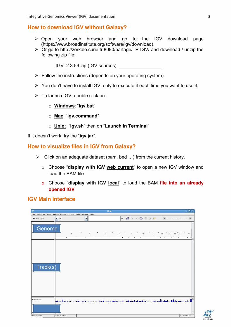
opened IGV IGV Main interface

Genome

Track(s)

Genome

Track(s)


Annotation Annotation


¾ You can add as many tracks as you want. They don’t need to be of the same type or format: you can combine a ChIP-seq enrichment track (bigwig) and the corresponding alignment track (bam) IF they were processed on the same reference genome. �

�You can access the Online help by clicking on “Help” in the bar menu then on “User Guide”. A basic tutorial is also accessible in “Help” then in “Tutorial”. Several training datasets are available in “File”>”Load data from Server”. � Interface with 2 datasets (Chip-Seq peaks & alignments) Thorvaldsdóttir H et al. Brief Bioinform 2013;14:178-192 Reference Genome ¾ Choose a genome already available in the Reference Genome Selector

(Human, Mouse, Yeast...) /!\ Be careful with the assembly (hg19 != hg18) /!\ ��

x IGV isn’t designed for unassembled references (thousands of contigs) ��¾ Load your own genome: in the bar menu, click on «Genomes» then on ��

« Load genome from File». Your genome should be an indexed FASTA2 file (.fa or .fasta)

2 An indexed FASTA is a FASTA file accompanied by its index file (a .fai file)


¾�You can also load a genome from an URL or a server. Ex. human genome hg18 (showing all chromosomes by default) Navigation ¾�You can�visualize 1 chromosome (ex: chr10) on this selector:

¾ The whole chromosome is shown by default. You can specify a genomic

range (chr10: 18000000-18150000) or a term (BEND2) in the search box. Then click on «Go» or press “Enter”. �

/!\ It can be any term present in the loaded annotation tracks: a gene (BRCA1) or transcript name (NM_007294) but also the interval names from a loaded BED file. ��

¾ 2 options to zoom in ��

¾ By clicking on the «+» (respectively «-» to zoom out) in the zoom bar �

¾ By choosing a range on the ruler: left-click at one point, hold it while moving your cursor to the right. �

�¾ To move on the chromosome: click on the left & right arrows �


¾ Click on the genomic coordinates or on the chromosome ideogram ��

¾ Click & Drag on the tracks to move around the region you selected ��¾ Go back to whole genome view �

��¾ Save an image of your current view �

�¾ Click on «File» then on «Save Image» �

�¾ Choose the format of your picture �

�• .png or .jpg

• .svg: vector graphics that can be modified in Illustrator or Inkscape

¾ Jump from one interval to the next one: in “File>Load from File”, select a

Bed File. Once loaded, left click on the name of the bed track (it should appear gray) then simultaneously click on the “ctrl” and “f” keys to jump to the next interval (very useful to visualize variants or enriched regions) �

�¾ Region Navigator: �

�¾ Import regions of interest in BED format (4 tabulated columns: chr start

end name) by clicking on “Region > Import Region” in the top menu ��

¾ Save the regions you found by clicking on this icon: �

Then click on each side of the region of interest (one click on the track to

open it on the left, one click on the track to close it on the right). A red bar appears just under the ruler to highlight the region you selected. Click on this red

bar then on “edit description” to give it a name. To find this region again, go to

“Regions > Region navigator”, select your interval then click on “View”.

¾ Export saved regions in BED format by clicking on “Regions > Export regions” �

�¾ In “Regions>Gene lists”, you can import/export your own gene lists or

use available ones. ��¾ Multiple view option: �

�¾ Enter several localization or terms in the search box (space separated).

Ex: BRCA1 BRCA2 RB1 or chr17:15000 chr18:10990 chr1:4500-4600��


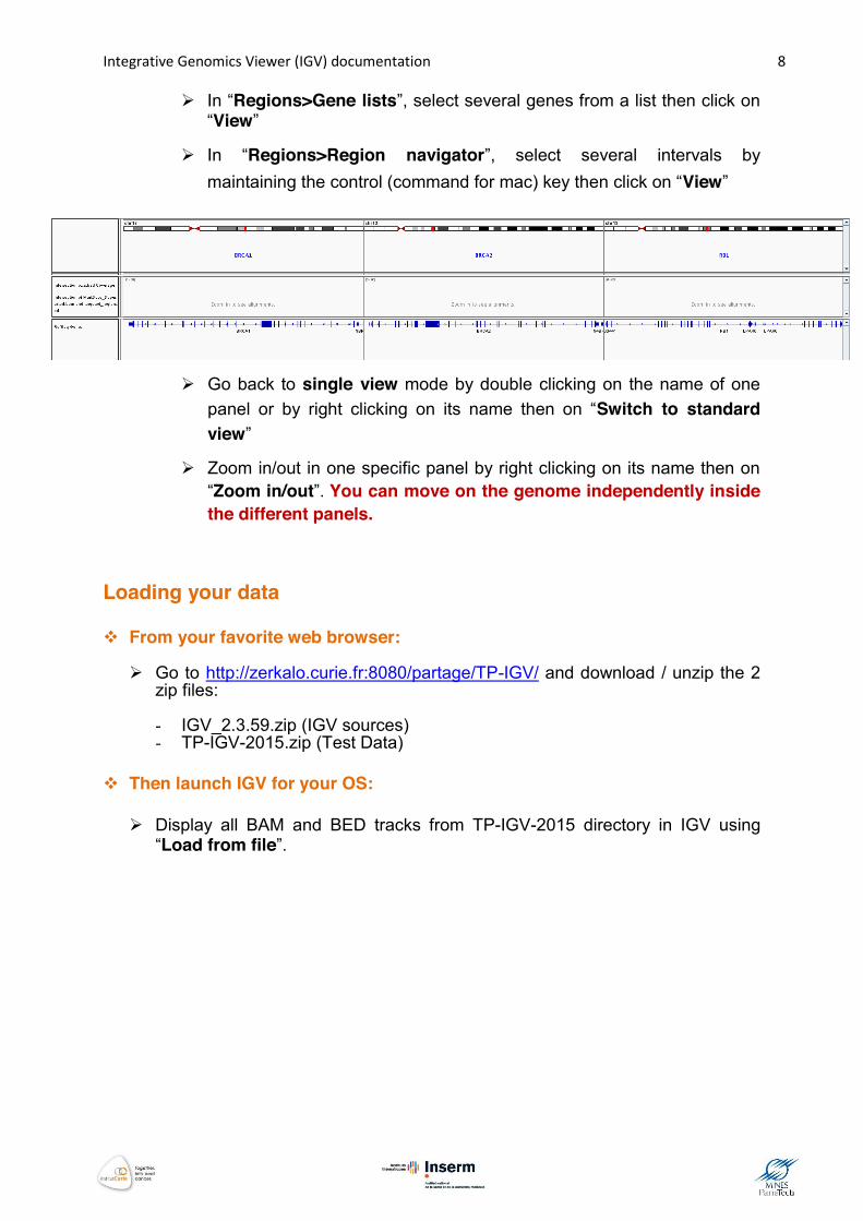
¾ In “Regions>Gene lists”, select several genes from a list then click on “View” �

¾ In “Regions>Region navigator”, select several intervals by maintaining the control (command for mac) key then click on “View” �

��¾ Go back to single view mode by double clicking on the name of one

panel or by right clicking on its name then on “Switch to standard view” �

�¾ Zoom in/out in one specific panel by right clicking on its name then on

“Zoom in/out”. You can move on the genome independently inside the different panels. �

��

Loading your data � From your favorite web browser: � ¾ Go to http://zerkalo.curie.fr:8080/partage/TP-IGV/ and download / unzip the 2

zip files:

- IGV_2.3.59.zip (IGV sources) - TP-IGV-2015.zip (Test Data)

�� Then launch IGV for your OS: � ��¾ Display all BAM and BED tracks from TP-IGV-2015 directory in IGV using

“Load from file”.

http://zerkalo.curie.fr:8080/partage/TP-IGV/


Graphical options Depending on the file format, some graphical options will be available by right clicking on the track.

• For annotations tracks (bed, gtf, wig...): you can change the color of the track and specify a visualization mode (collapsed, expanded and squished). The collapsed mode might hide annotations that overlay on each other so be sure to put the expanded mode on (i.e.: for the RefSeq Genes track, you need the expanded mode to see all available isoforms).

• For alignment tracks (BAM): multiples options are available, depending on

your type of data. Some may help you have a better understanding of your data. You can try all of the options but here are the most useful ones:

• Color alignment by

o Strand: to visually check if a variant has a strand bias

o First of pair strand: to visually check if you have a directional

RNA-seq

o Insert-size / insert-size and pair orientation: to identify structural variations like inversion, duplication or translocation

o Bisulfite mode: to correctly see your bisulfite-seq/methyl-seq

data

• Sort alignment by base: to reorder the alignments at a specific position by base can help visualize a variant

• Show mismatches bases: to see variations from the reference in the

alignments

• View as pairs: link paired-end alignments together

• View mate region in split screen: useful to visualize translocation events (pairs mapped on different chromosomes)

• Visualization mode: expanded is always a good choice to see more

details but the collapsed mode can be useful to see Chip-seq peaks.

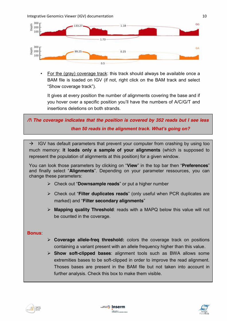
• Sashimi-plot (RNA-seq only, see example below): a very useful visualization tool (no isoform prediction is done) to see junctions between exons for RNA-seq data and have an idea of the number of spanning reads at a specific junction.


• For the (gray) coverage track: this track should always be available once a BAM file is loaded on IGV (if not, right click on the BAM track and select “Show coverage track”).

It gives at every position the number of alignments covering the base and if you hover over a specific position you’ll have the numbers of A/C/G/T and insertions deletions on both strands.

/!\ The coverage indicates that the position is covered by 352 reads but I see less

than 50 reads in the alignment track. What’s going on?

Æ�IGV has default parameters that prevent your computer from crashing by using too much memory: it loads only a sample of your alignments (which is supposed to represent the population of alignments at this position) for a given window.

You can look those parameters by clicking on “View” in the top bar then “Preferences” and finally select “Alignments”. Depending on your parameter ressources, you can change these parameters:

¾ Check out “Downsample reads” or put a higher number �

�¾ Check out “Filter duplicates reads” (only useful when PCR duplicates are

marked) and “Filter secondary alignments” ��

¾ Mapping quality Threshold: reads with a MAPQ below this value will not be counted in the coverage.

Bonus: ¾ Coverage allele-freq threshold: colors the coverage track on positions

containing a variant present with an allele frequency higher than this value. ¾ Show soft-clipped bases: alignment tools such as BWA allows some

extremities bases to be soft-clipped in order to improve the read alignment. Thoses bases are present in the BAM file but not taken into account in further analysis. Check this box to make them visible.


Examples

1. Visualization of variants in DNA-seq data

x Don’t forget to always sort reads by base at a variant position and to load a bed file containing the variants position and their names in order to easily search for one. � �

x Mismatched bases from the reference are shown in a different color (each base has its own color).��

x Base counts indicated by hovering on the coverage track at the variant position can help assess the variant allelic ratio. The decomposition on the forward/reverse strands can help determine a potential strand bias: when a base is covered by the same amount of forward and reverse alignments (blue and pink) and the variant is supported by a high proportion of one type of strand (ie: 90%), it might be an artifact. �

x This purple bar is the symbol for an insertion (hover over it to view the inserted bases) (ex: variant240)

x Deletions are indicated by a blank space crossed by a

black line like this (ex: variant230):


2. Visualization of RNA-seq data with the sashimi-plot view

• Focus on the OAS1 gene. If you see the “Zoom in to see alignments’ message, zoom in until you see alignments.

• Set the track in its collapsed mode. The blue lines link the different parts of a spanning read that, by definition, map on several exons. Zoom in on the two last exons of OAS1 then sort the alignments by base just before the last exon. You can see alignments outside of the known exons of this gene. This alternative isoform is caused by the mutation in the splice site at chr12:113,357,193 (Pickrell et al,2012)

• Right click on the track, select “sashimi-plot”. You’ll see the coverage on every exons and lines joining the exons with a number specifying the number of spanning reads for this junction. You can zoom in the last two exons, move on the track and click on a specific exon (in blue) to only see junctions involving this exon (click on an intron to see everything).


• 31 reads span the junction of exon 5 and the cryptic 3’ splice site upstream of the mutation

• Some options are available by right clicking on the sashimi:

¾ Set color: to distinguish between different tracks

¾ Save image: to save your sashimi (svg format is recommended for high

resolution picture and can be modified using illustrator or inkscape)

¾ Set min junction coverage: alignment data are noisy and there are a

lot of junctions with a low number of spanning reads. Put a higher

number of minimal junction coverage to only see the higher

represented junctions.

/!\ Sashimi plots are very useful to get a descriptive view of RNA-seq data but cannot replace a proper analysis : it’s only a visualization tool. /!\

3. Visualization of the Transcription Factor GATA-3 BindingSites by ChIP-

seq from ENCODE

ChIP-seq data from the ENCODE project are used in this part in order to observe at the same time a BAM file containing the reads alignments and a BED file containing the enriched regions of high read density (peaks) identified by the bioinformatics analysis. These peaks correspond to the predicted binding sites of the studied transcription factor, GATA-3 in the Mcf7 cell line. ¾ On IGV, enter the coordinates “chr2:190,349,400-190,354,600” or enter the

name of the peak “peak20645”. You’ll see 2 tracks, one corresponding to the signal and the other to the identified peaks. �


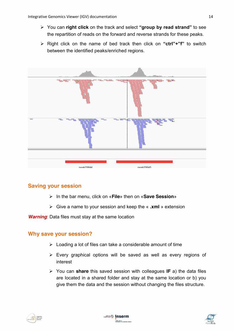
¾ You can right click on the track and select “group by read strand” to see the repartition of reads on the forward and reverse strands for these peaks. �

�¾ Right click on the name of bed track then click on “ctrl”+”f” to switch

between the identified peaks/enriched regions. � Saving your session

¾ In the bar menu, click on «File» then on «Save Session» ��

¾ Give a name to your session and keep the « .xml » extension � Warning: Data files must stay at the same location Why save your session?

¾ Loading a lot of files can take a considerable amount of time ��

¾ Every graphical options will be saved as well as every regions of interest �

�¾ You can share this saved session with colleagues IF a) the data files

are located in a shared folder and stay at the same location or b) you give them the data and the session without changing the files structure. �

Visualization of Next Generation Sequencing Data using the Integrative...

Documents

Transcript of Visualization of Next Generation Sequencing Data using the Integrative...