VISUAL FEATURE LEARNING - Universität Innsbruck

VISUAL FEATURE LEARNING

A Dissertation Presented

by

JUSTUS H. PIATER

Submitted to the Graduate School of theUniversity of Massachusetts Amherst in partial fulfillment

of the requirements for the degree of

DOCTOR OF PHILOSOPHY

February 2001 (revised June 14, 2001)

Department of Computer Science

c© Copyright by Justus H. Piater 2001All Rights Reserved


A Dissertation Presented

by

JUSTUS H. PIATER

Approved as to style and content by:

Roderic A. Grupen, Chair

Edward M. Riseman, Member

Andrew H. Fagg, Member

Neil E. Berthier, Member

James F. Kurose, Department ChairDepartment of Computer Science

For my daughter Zoe,born 3 days and 18 hours after my dissertation defense,

her siblings, Bennett and Talia,and my wife Petra.

I will love you all forever!

ACKNOWLEDGMENTS

Few substantial pieces of work are the achievement of a single person. This dissertation is noexception. Many people have contributed to its development. First of all, this endeavor wouldhave been impossible without the continual support of my wife Petra. She walked many extramiles and backed me during times of highly concentrated effort. I love you! I also thank mythree children, who – one after the other – emerged on the scene during my five years of graduatestudies at the University of Massachusetts. They always wanted me to be home with them allday. Forgive me for having a job! Bennett in particular has unknowingly made his contributionsto this research. The way he learned to recognize hand-drawnshapes during his early years wasvery inspiring.

I am indebted to my advisor Rod Grupen for many inspiring discussions, unshakable confi-dence, his vision for task-driven learning by interaction,and for simply being a great guy. Thankyou for inviting me into your lab! The first ideas about visuallearning grew out of my earlierwork with Ed Riseman. He has been a constant source of encouragement, and his keen observa-tions and suggestions have greatly improved the quality of this presentation. Great credit is dueto Andy Fagg, who has reviewed the ideas and their presentation with unparalleled scrutiny, andsuggested many insightful improvements. Of course, I am to blame for any remaining errors.Thanks to their valuable feedback, this dissertation turned into a picture book that includes 336individual graphics files in 62 figures.

I am grateful to Paul Utgoff for sharing his insight during numerous discussions of machinelearning issues that have shaped my thinking forever. He introduced me to the Kolmogorov-Smirnoff distance that serves several pivotal roles in this work. I deeply regret that we never gotaround to playing music together! Special thanks go to the psychologists Rachel Clifton andNeil Berthier who introduced me to the world of human perceptual development and learning.This had a strong impact on my research interests, and has greatly enhanced the interdisciplinaryaspects of this dissertation. Their sharp insights have added great value to my studies.

On the more mundane side, I acknowledge the helpful support of Hugin A/S. Hey Danes,neighbors! They provided me with a low-cost Ph.D. license oftheir Bayesian network library forSolaris, and later with a Linux port. This library was used inthe implementation of the systemdescribed in Chapters 4 and 5. I also want to use this opportunity to express my appreciationof the Free Software/ Open Source community, whose efforts have produced some of the bestsoftware in existence. Without Linux and many GNU tools, my life would be considerablyharder. I wonder how people ever lived without Emacs? Thanksto the excellent LATEX 2εclass file by my fellow graduate student John Ridgway (that builds on code contributed by RodGrupen, and others), this document looks about as nice as ourGraduate School allowsip p .

Many friends and colleagues helped make my time at the UMass Computer Science depart-ment very pleasant. The Laboratory of Perceptual Robotics is a wonderful bunch of creativepeople. Thanks to Elizeth for reminding me of my own birthdayso the lab would get theirwell-deserved cake. She and her co-veterans Jefferson and Manfred take most of the credit formaking LPR a great place to hang out. Their successors in the lab now have to start over. Andthanks to my wife for baking those cakes. I think they will be remembered longer than I. Thanksto my South-American and Italian friends for restoring my sanity by dragging me away from mydesk and onto the soccer field. I apologize to my fellow grads from LPR, ANW, and EKSL, asmy floods of long-running experiments left them with few clock cycles on our shared computecluster. A big thank-you goes to my special friends and brothers in Christ, Craig the scientist

v

and Achim the musician, for being there for me in my joys and sorrows. How empty would lifebe without true friends!

Most of all, I want to thank God for calling our world into being. It is so wonderfully richand complex that no one but You will ever fully understand it.Exploring the why’s and how’sof physics and life makes for a fulfilled professional life. The more I learn about Your creation,the more I am in awe. My life belongs to You.

O Lord, how manifold are Your works!In wisdom You have made them all.

Psalm 104:24

vi

ABSTRACT


FEBRUARY 2001 (REVISED JUNE 14, 2001)

JUSTUS H. PIATER

Dipl.-Inform., UNIVERSITY OF MAGDEBURG, GERMANY

M.Sc., UNIVERSITY OF MASSACHUSETTS AMHERST

Ph.D., UNIVERSITY OF MASSACHUSETTS AMHERST

Directed by: Professor Roderic A. Grupen

Humans learn robust and efficient strategies for visual tasks through interaction withtheirenvironment. In contrast, most current computer vision systems have no such learning capa-bilities. Motivated by insights from psychology and neurobiology, I combine machine learningand computer vision techniques to develop algorithms for visual learning in open-ended tasks.Learning is incremental and makes only weak assumptions about the task environment.

I begin by introducing an infinite feature space that contains combinations of local edge andtexture signatures not unlike those represented in the human visual cortex. Such features canexpress distinctions over a wide range of specificity or generality. The learning objective is toselect asmallnumber ofhighly usefulfeatures from this space in a task-driven manner. Featuresare learned by general-to-specific random sampling. This isillustrated on two different tasks,for which I give very similar learning algorithms based on the same principles and the samefeature space.

The first system incrementally learns to discriminate visual scenes. Whenever it fails to rec-ognize a scene, new features are sought that improve discrimination. Highly distinctive featuresare incorporated into dynamically updated Bayesian network classifiers. Even after all recog-nition errors have been eliminated, the system can continueto learn better features, resemblingmechanisms underlying human visual expertise. This tends to improve classification accuracyon independent test images, while reducing the number of features used for recognition.

In the second task, the visual system learns to anticipate useful hand configurations fora haptically-guided dextrous robotic grasping system, much like humans do when they pre-shape their hand during a reach. Visual features are learnedthat correlate reliably with theorientation of the hand. A finger configuration is recommended based on the expected graspquality achieved by each configuration.

The results demonstrate how a largely uncommitted visual system can adapt and specializeto solve particular visual tasks. Such visual learning systems have great potential in applicationscenarios that are hard to model in advance, e.g. autonomousrobots operating in natural envi-ronments. Moreover, this dissertation contributes to our understanding of human visual learningby providing a computational model of task-driven development of feature detectors.

vii

TABLE OF CONTENTS

Page

ACKNOWLEDGMENTS . . . . . . . . . . . . . . . . . . . . . . . . . . . . . . . . . . . . v

ABSTRACT . . . . . . . . . . . . . . . . . . . . . . . . . . . . . . . . . . . . . . . . . . .vii

LIST OF TABLES . . . . . . . . . . . . . . . . . . . . . . . . . . . . . . . . . . . . . . . .xiii

LIST OF FIGURES . . . . . . . . . . . . . . . . . . . . . . . . . . . . . . . . . . . . . . .xv

CHAPTER

1. INTRODUCTION . . . . . . . . . . . . . . . . . . . . . . . . . . . . . . . . . . . . . . 11.1 Closed and Open Task Domains . . . . . . . . . . . . . . . . . . . . . . . .. . . . 11.2 Scope . . . . . . . . . . . . . . . . . . . . . . . . . . . . . . . . . . . . . . . . . . 21.3 Outline . . . . . . . . . . . . . . . . . . . . . . . . . . . . . . . . . . . . . . . . . 3

2. THIS WORK IN PERSPECTIVE . . . . . . . . . . . . . . . . . . . . . . . . . . . . . 52.1 Human Visual Skill Learning . . . . . . . . . . . . . . . . . . . . . . . .. . . . . . 52.2 Machine Perceptual Skill Learning . . . . . . . . . . . . . . . . . .. . . . . . . . . 62.3 Objective . . . . . . . . . . . . . . . . . . . . . . . . . . . . . . . . . . . . . . .. 82.4 Motivation . . . . . . . . . . . . . . . . . . . . . . . . . . . . . . . . . . . . . .. . 10

3. AN UNBOUNDED FEATURE SPACE . . . . . . . . . . . . . . . . . . . . . . . . . . . 113.1 Related Work . . . . . . . . . . . . . . . . . . . . . . . . . . . . . . . . . . . . .. 113.2 Objective . . . . . . . . . . . . . . . . . . . . . . . . . . . . . . . . . . . . . . .. 123.3 Background . . . . . . . . . . . . . . . . . . . . . . . . . . . . . . . . . . . . . .. 13

3.3.1 Gaussian-Derivative Filters . . . . . . . . . . . . . . . . . . . .. . . . . . . 143.3.2 Steerable Filters . . . . . . . . . . . . . . . . . . . . . . . . . . . . . .. . 153.3.3 Scale-Space Theory . . . . . . . . . . . . . . . . . . . . . . . . . . . . .. 16

3.4 Primitive Features . . . . . . . . . . . . . . . . . . . . . . . . . . . . . . .. . . . . 193.4.1 Edgels . . . . . . . . . . . . . . . . . . . . . . . . . . . . . . . . . . . . . . 203.4.2 Texels . . . . . . . . . . . . . . . . . . . . . . . . . . . . . . . . . . . . . . 203.4.3 Salient Points . . . . . . . . . . . . . . . . . . . . . . . . . . . . . . . . .. 213.4.4 Feature Responses and the Value of a Feature . . . . . . . . .. . . . . . . . 24

3.5 Compound Features . . . . . . . . . . . . . . . . . . . . . . . . . . . . . . . .. . . 253.5.1 Geometric Composition . . . . . . . . . . . . . . . . . . . . . . . . . .. . 253.5.2 Boolean Composition . . . . . . . . . . . . . . . . . . . . . . . . . . . .. 26

3.6 Discussion . . . . . . . . . . . . . . . . . . . . . . . . . . . . . . . . . . . . . .. . 27

ix

4. LEARNING DISTINCTIVE FEATURES . . . . . . . . . . . . . . . . . . . . . . . . . 294.1 Related Work . . . . . . . . . . . . . . . . . . . . . . . . . . . . . . . . . . . . .. 294.2 Objective . . . . . . . . . . . . . . . . . . . . . . . . . . . . . . . . . . . . . . .. 304.3 Background . . . . . . . . . . . . . . . . . . . . . . . . . . . . . . . . . . . . . .. 32

4.3.1 Classification Using Bayesian Networks . . . . . . . . . . . .. . . . . . . . 324.3.2 Kolmogorov-Smirnoff Distance . . . . . . . . . . . . . . . . . . . . . . . . 34

4.4 Feature Learning . . . . . . . . . . . . . . . . . . . . . . . . . . . . . . . . .. . . 344.4.1 Classifier . . . . . . . . . . . . . . . . . . . . . . . . . . . . . . . . . . . . 354.4.2 Recognition . . . . . . . . . . . . . . . . . . . . . . . . . . . . . . . . . . .384.4.3 Feature Learning Algorithm . . . . . . . . . . . . . . . . . . . . . .. . . . 404.4.4 Impact of a New Feature . . . . . . . . . . . . . . . . . . . . . . . . . . .. 44

4.5 Experiments . . . . . . . . . . . . . . . . . . . . . . . . . . . . . . . . . . . . .. . 454.5.1 The COIL Task . . . . . . . . . . . . . . . . . . . . . . . . . . . . . . . . . 464.5.2 The Plym Task . . . . . . . . . . . . . . . . . . . . . . . . . . . . . . . . . 524.5.3 The Mel Task . . . . . . . . . . . . . . . . . . . . . . . . . . . . . . . . . . 56

4.6 Discussion . . . . . . . . . . . . . . . . . . . . . . . . . . . . . . . . . . . . . .. . 59

5. EXPERT LEARNING . . . . . . . . . . . . . . . . . . . . . . . . . . . . . . . . . . . .635.1 Related Work . . . . . . . . . . . . . . . . . . . . . . . . . . . . . . . . . . . . .. 635.2 Objective . . . . . . . . . . . . . . . . . . . . . . . . . . . . . . . . . . . . . . .. 645.3 Expert Learning Algorithm . . . . . . . . . . . . . . . . . . . . . . . . .. . . . . . 645.4 Experiments . . . . . . . . . . . . . . . . . . . . . . . . . . . . . . . . . . . . .. . 65

5.4.1 The COIL Task . . . . . . . . . . . . . . . . . . . . . . . . . . . . . . . . . 665.4.2 The Plym Task . . . . . . . . . . . . . . . . . . . . . . . . . . . . . . . . . 745.4.3 The Mel Task . . . . . . . . . . . . . . . . . . . . . . . . . . . . . . . . . . 755.4.4 Incremental Tasks . . . . . . . . . . . . . . . . . . . . . . . . . . . . . .. 825.4.5 Computational Demands . . . . . . . . . . . . . . . . . . . . . . . . . .. . 94

5.5 Discussion . . . . . . . . . . . . . . . . . . . . . . . . . . . . . . . . . . . . . .. . 95

6. LEARNING FEATURES FOR GRASP PRE-SHAPING . . . . . . . . . . . . . . . . 976.1 Related Work . . . . . . . . . . . . . . . . . . . . . . . . . . . . . . . . . . . . .. 976.2 Objective . . . . . . . . . . . . . . . . . . . . . . . . . . . . . . . . . . . . . . .. 976.3 Background . . . . . . . . . . . . . . . . . . . . . . . . . . . . . . . . . . . . . .. 98

6.3.1 Haptically-Guided Grasping . . . . . . . . . . . . . . . . . . . . .. . . . . 986.3.2 The von Mises Distribution . . . . . . . . . . . . . . . . . . . . . . .. . . . 100

6.4 Feature Learning . . . . . . . . . . . . . . . . . . . . . . . . . . . . . . . . .. . . 1006.4.1 Fitting a Parametric Orientation Model . . . . . . . . . . . .. . . . . . . . 1036.4.2 Selecting Object-Specific Data Points . . . . . . . . . . . . .. . . . . . . . 1046.4.3 Predicting the Quality of a Grasp . . . . . . . . . . . . . . . . . .. . . . . . 1056.4.4 Feature Learning Algorithm . . . . . . . . . . . . . . . . . . . . . .. . . . 106

6.5 Experiments . . . . . . . . . . . . . . . . . . . . . . . . . . . . . . . . . . . . .. . 1086.5.1 Training Visual Models . . . . . . . . . . . . . . . . . . . . . . . . . .. . . 1096.5.2 Using Visual Models to Cue Haptic Grasping . . . . . . . . . .. . . . . . . 110

6.6 Discussion . . . . . . . . . . . . . . . . . . . . . . . . . . . . . . . . . . . . . .. . 114

7. CONCLUSIONS . . . . . . . . . . . . . . . . . . . . . . . . . . . . . . . . . . . . . . .1177.1 Summary of Contributions . . . . . . . . . . . . . . . . . . . . . . . . . .. . . . . 1177.2 Future Directions . . . . . . . . . . . . . . . . . . . . . . . . . . . . . . . .. . . . 119

7.2.1 Primitive Features and their Composition . . . . . . . . . .. . . . . . . . . 1197.2.2 Higher-Level Features . . . . . . . . . . . . . . . . . . . . . . . . . .. . . 1207.2.3 Efficient Feature Search . . . . . . . . . . . . . . . . . . . . . . . . . . . . 120

x

7.2.4 Redundancy . . . . . . . . . . . . . . . . . . . . . . . . . . . . . . . . . . . 1207.2.5 Integrating Visual Skills . . . . . . . . . . . . . . . . . . . . . . .. . . . . 121

7.3 Uncommitted Learning in Open Environments . . . . . . . . . . .. . . . . . . . . . 121

APPENDIX: EXPECTATION-MAXIMIZATION FOR VON MISES MIXTURE S . . . . 123

BIBLIOGRAPHY . . . . . . . . . . . . . . . . . . . . . . . . . . . . . . . . . . . . . . . .125

xi

LIST OF TABLES

Table Page

1.1 Typical characteristics of closed vs. open task domains. . . . . . . . . . . . . . . . . 2

2.1 Summary of important characteristics of the two applications discussed in thisdissertation. . . . . . . . . . . . . . . . . . . . . . . . . . . . . . . . . . . . . . 9

4.1 Selecting true and mistaken classes using posterior class probabilities. . . . . . . . . 42

4.2 Summary of empirical results on all three tasks. . . . . . . .. . . . . . . . . . . . . 47

4.3 Results on the COIL task. . . . . . . . . . . . . . . . . . . . . . . . . . . .. . . . . 48

4.4 Results on the COIL task: Confusion matrices of ambiguous recognitions. . . . . . . 49

4.5 Results on the Plym task. . . . . . . . . . . . . . . . . . . . . . . . . . . .. . . . . 55

4.6 Results on the Plym task: Confusion matrices of ambiguous recognitions. . . . . . . 56

4.7 Results on the Mel task. . . . . . . . . . . . . . . . . . . . . . . . . . . . .. . . . . 58

4.8 Results on the Mel task: Confusion matrices of ambiguousrecognitions. . . . . . . . 59

5.1 Summary of empirical results after expert learning on all tasks. . . . . . . . . . . . . 67

5.2 Results on the COIL task after Expert Learning. . . . . . . . .. . . . . . . . . . . . 71

5.3 Results on the COIL task after Expert Learning: Confusion matrices of ambiguousrecognitions. . . . . . . . . . . . . . . . . . . . . . . . . . . . . . . . . . . . . . 74

5.4 Results on the Plym task after Expert Learning. . . . . . . . .. . . . . . . . . . . . 77

5.5 Results on the Plym task after Expert Learning: Confusion matrices of ambiguousrecognitions. . . . . . . . . . . . . . . . . . . . . . . . . . . . . . . . . . . . . . 78

5.6 Results on a two-class Plym subtask after 15-fold ExpertLearning. . . . . . . . . . . 78

5.7 Results on the Mel task after Expert Learning. . . . . . . . . .. . . . . . . . . . . . 81

5.8 Results on the Mel task after Expert Learning: Confusionmatrices of ambiguousrecognitions. . . . . . . . . . . . . . . . . . . . . . . . . . . . . . . . . . . . . . 82

xiii

5.9 Results on a two-class Mel subtask after 12-fold Expert Learning. . . . . . . . . . . 83

xiv

LIST OF FIGURES

Figure Page

2.1 A general model of incremental feature learning. . . . . . .. . . . . . . . . . . . . 8

3.1 “Eigen-faces” – eigenvectors corresponding to the eight largest eigenvalues of a set offace images. . . . . . . . . . . . . . . . . . . . . . . . . . . . . . . . . . . . . . 11

3.2 Visualization of a two-dimensional Gaussian function and some oriented derivatives(cf. Equation 3.3). . . . . . . . . . . . . . . . . . . . . . . . . . . . . . . . . . .14

3.3 Example manipulations with first-derivative images. . .. . . . . . . . . . . . . . . . 16

3.4 Visualization of a linear scale space generated by smoothing with Gaussian kernels ofincreasing standard deviation. . . . . . . . . . . . . . . . . . . . . . . .. . . . . 16

3.5 Example of a scale functions(σ). . . . . . . . . . . . . . . . . . . . . . . . . . . . . 17

3.6 Illustration of the 200 strongest scale-space maxima ofsblob(σ). . . . . . . . . . . . 18

3.7 Illustration of scale-space maxima ofscorner(σ). . . . . . . . . . . . . . . . . . . . . 19

3.8 Extracting edges from the projected scale space. . . . . . .. . . . . . . . . . . . . . 21

3.9 Salient edgels and texels extracted from an example image. . . . . . . . . . . . . . . 22

3.10 Stability of texels across viewpoints. . . . . . . . . . . . . .. . . . . . . . . . . . . 23

3.11 Matching a texel (a) across rotation and scale, without(b) and with (c) rotationalnormalization. . . . . . . . . . . . . . . . . . . . . . . . . . . . . . . . . . . . . 24

3.12 A geometric compound feature consisting of three primitive features. . . . . . . . . . 26

4.1 Definition of the Kolmogorov-Smirnoff distance. . . . . . . . . . . . . . . . . . . . 34

4.2 A model of incremental discrimination learning (cf. Figure 2.1, page 8). . . . . . . . 35

4.3 A hypothetical example Bayesian network. . . . . . . . . . . . .. . . . . . . . . . 36

4.4 Highly uneven and overlapping feature value distributions. . . . . . . . . . . . . . . 37

4.5 KSD of a featuref that, if not found in an image, causes its Bayesian network toinferthat its class is absent with absolute certainty. . . . . . . . . .. . . . . . . . . . 45

xv

4.6 Objects used in the COIL task. . . . . . . . . . . . . . . . . . . . . . . .. . . . . . 46

4.7 Examples of features learned for the COIL task. . . . . . . . .. . . . . . . . . . . . 50

4.8 Features characteristic ofobj1 located in all images of this class where they arepresent. . . . . . . . . . . . . . . . . . . . . . . . . . . . . . . . . . . . . . . . 51

4.9 Spatial distribution of feature responses of selected features characteristic ofobj1(left columns), for comparison also shown forobj4 (right columns). . . . . . . . 53

4.10 Objects used in the Plym task. . . . . . . . . . . . . . . . . . . . . . .. . . . . . . 54

4.11 Examples of features learned for the Plym task. . . . . . . .. . . . . . . . . . . . . 54

4.12 All images used in the Mel task. . . . . . . . . . . . . . . . . . . . . .. . . . . . . 57

4.13 Examples of features learned for the Mel task. . . . . . . . .. . . . . . . . . . . . . 60

5.1 Expert Learning results on the COIL task. . . . . . . . . . . . . .. . . . . . . . . . 68

5.2 Examples of expert features learned for the COIL task, Fold 1. . . . . . . . . . . . . 70

5.3 Expert Features characteristic ofobj1 located in all images of this class where theyare present. . . . . . . . . . . . . . . . . . . . . . . . . . . . . . . . . . . . . . 72

5.4 Spatial distribution of expert feature responses of allfeatures characteristic ofobj1learned in Fold 1 (left columns), for comparison also shown for obj4 (rightcolumns). . . . . . . . . . . . . . . . . . . . . . . . . . . . . . . . . . . . . . . 73

5.5 Variation due to randomness in the learning procedure. .. . . . . . . . . . . . . . . 75

5.6 Expert Learning results on the Plym task. . . . . . . . . . . . . .. . . . . . . . . . 76

5.7 Examples of expert features learned for the Plym task, Fold 1. . . . . . . . . . . . . 79

5.8 Expert Learning results on the Mel task. . . . . . . . . . . . . . .. . . . . . . . . . 80

5.9 Examples of expert features learned for the Mel task, Fold 1. . . . . . . . . . . . . . 83

5.10 Objects used in the 10-object COIL task. . . . . . . . . . . . . .. . . . . . . . . . . 85

5.11 Incremental Expert Learning results on the COIL-inc task, Fold 1. . . . . . . . . . . 86

5.12 Incremental Expert Learning results on the COIL-inc task, Fold 2. . . . . . . . . . . 87

5.13 Numbers of features sampled during the COIL-inc task. .. . . . . . . . . . . . . . . 88

5.14 Incremental Expert Learning results on the Plym-inc task, Fold 1. . . . . . . . . . . 89

5.15 Incremental Expert Learning results on the Plym-inc task, Fold 2. . . . . . . . . . . 90

xvi

5.16 Numbers of features sampled during the Plym-inc task. .. . . . . . . . . . . . . . . 91

5.17 Incremental Expert Learning results on the Mel-inc task, Fold 1. . . . . . . . . . . . 92

5.18 Incremental Expert Learning results on the Mel-inc task, Fold 2. . . . . . . . . . . . 93

5.19 Number of features sampled for various tasks, plotted versus the number ofclasses. . . . . . . . . . . . . . . . . . . . . . . . . . . . . . . . . . . . . . . . 95

6.1 Grasp synthesis as closed-loop control. (Reproduced with permission from Coelhoand Grupen [21].) . . . . . . . . . . . . . . . . . . . . . . . . . . . . . . . . . . 98

6.2 The Stanford/JPL dextrous hand performing haptically-guided closed-loop graspsynthesis. . . . . . . . . . . . . . . . . . . . . . . . . . . . . . . . . . . . . . . 99

6.3 Object wrench phase portraits traced during grasp syntheses. . . . . . . . . . . . . . 99

6.4 A hypothetical phase portrait of a native controllerπc (left) and all possible contexttransitions (right). . . . . . . . . . . . . . . . . . . . . . . . . . . . . . . . .. . 100

6.5 Illustration of four von Mises probability densities ona circular domain. . . . . . . . 101

6.6 Scenario for learning features to recommend grasp parameters (cf. Figure 2.1,page 8). . . . . . . . . . . . . . . . . . . . . . . . . . . . . . . . . . . . . . . . 102

6.7 Definition of the hand orientation (azimuthal angle) fortwo- and three-fingeredgrasps. . . . . . . . . . . . . . . . . . . . . . . . . . . . . . . . . . . . . . . . . 102

6.8 By Coelho’s formulation, some objects are better grasped with two fingers (a), somewith three (b), and for some this choice is unimportant (c, d). . . . . . . . . . . . 102

6.9 Left: Data points induced by a given feature on various images of an object formstraight lines on a torus (two in this case); right: A mixtureof two von Misesdistributions was fitted to these data. . . . . . . . . . . . . . . . . . .. . . . . . 103

6.10 Kolmogorov-Smirnoff distance KSDf between the conditional distributions of featureresponse magnitudes given correct and false predictions. .. . . . . . . . . . . . 105

6.11 Representative examples of synthesized objects and converged simulated graspconfigurations using Coelho’s haptically-guided graspingsystem. . . . . . . . . . 109

6.12 Example views of objects used in the grasping simulations. . . . . . . . . . . . . . . 109

6.13 Quantitative results of hand orientation prediction.. . . . . . . . . . . . . . . . . . . 110

6.14 Results on two-fingered grasps of cubes (top half), and three-fingered grasps oftriangular prisms (bottom half). . . . . . . . . . . . . . . . . . . . . . .. . . . . 111

xvii

6.15 Examples of features obtained by training two-fingeredmodels on cubes andthree-fingered models on triangular prisms, using clean data separated by objecttype (cf. Figure 6.14). . . . . . . . . . . . . . . . . . . . . . . . . . . . . . . .. 112

6.16 Examples of features obtained by training two- and three-fingered models on cubesand triangular prisms, using a single dataset containing relatively noise-freegrasps of cubes and triangular prisms (cf. Figure 6.17). . . .. . . . . . . . . . . 113

6.17 Grasp results on cubes and triangular prisms. . . . . . . . .. . . . . . . . . . . . . 113

xviii

CHAPTER 1

INTRODUCTION

Humans have a remarkable ability to act reasonably based on perceptual information abouttheir environment. Our perceptual system functions with such speed and reliability that weare deluded into underestimating the complexity of everyday perceptual tasks. In particular,humans rely heavily on visual perception. We orient ourselves, recognize environments, objects,and people, and manipulate items based on vision without ever thinking about it. Given theimportance of vision to humans, it is not surprising that vision has been the most-studied modeof machine perception since the early days of artificial intelligence. Nevertheless, despite fiftyyears of active research in artificial intelligence, robotics and computer vision, many real-worldvisuomotor tasks remain that are easily performed by humansbut are still unsolved by machines.The robustness and versatility of biological sensorimotorinteraction cannot yet be matched inrobotic systems.

What is it that enables higher animals, first and foremost humans, to outperform machinesso dramatically on real-world visuomotor tasks? I believe that the answer is grounded in thefollowing two theses that form the basis of this dissertation:

• The human visual system isadaptive. During the first years of life, the visual capabilitiesof children increase dramatically. These capabilities arenot limited by the design of thevisual system alone, but are modified by learning. All throughout life, the human visualsystem continues to improve performance on both novel and well-practiced tasks.

In contrast, most current machine vision systems do not learn in this way. They aredesigned to perform, and their performance is limited by thedesign. They do not usuallyimprove over time or adapt to novel situations unforeseen bythe designer.

• The human visual system is inextricably linked with humanactivity. Activity operatesin synergy with vision and facilitates visual learning, andvision subserves activity. Hu-man vision operates in a highly task-dependent way and is tuned to deliver exactly theinformation needed.

In contrast, most research in computer vision has focused ontask-independent visualfunctionality. In a typical scenario, a computer vision system produces a generic result orrepresentation for use by subsequent processing stages.

Both of these points will be further discussed in Chapter 2. The remainder of this openingchapter serves to define the scope and organization of this dissertation.

1.1 Closed and Open Task Domains

The field of computer vision is commonly subdivided into low-level and high-level vision. Low-level vision is typically concerned with task-independentimage analysis such as edge extractionor computation of disparity or optical flow. High-level vision considers application-level prob-lems, e.g. object recognition or vision-guided grasping. Considerable progress has been madein both areas during the past decade. For example, machine recognition systems have achievedunprecedented levels of performance [73, 104, 71, 77, 78]. Increasingly impressive recognition

1

results are reported on large databases of various objects.Automated character recognition sys-tems are involved in sorting most of the U.S. mail. Optical biometric identification systems havereached commercial maturity.

While these successful systems are truly remarkable, most of them are designed for tasksthat are limited in scope and well defined at design time. For instance, most object recognitionsystems operate on a fixed set of known objects. Many algorithms in fact require access to acomplete set of training images during a dedicated trainingphase. Deployed OCR and biometricidentification systems operate under highly controlled conditions where parameters such as size,location, and approximate appearance of the visual target are known. Similar arguments can bemade for other computer vision problems such as face detection, terrain classification, or vision-guided navigation.

Task domains that share these characteristics I callclosed. I argue that many practical visionproblems are not closed. For instance, a human activity recognition system should be able to op-erate under many different lighting conditions and in a variety of contexts; indoors or outdoors,with any number of people in the scene. A visually navigated mobile robot should be able tolearn distinctive landmarks by itself. If the robot is movedfrom one environment to another, onedoes not want to redesign the recognition algorithm – the same algorithm should be applicablein, and adaptive to, a variety of environments. An autonomous robot that traverses unknownterrain or collects specimens should be able to learn to predict the effect of its actions based onperceptual information in order to improve its actions withgrowing experience. Ultimately, itshould be the interaction of an agent with its environment – as opposed to a supervisory trainingsignal – that drives the formation of perceptual capabilities while performing a task [67, 114].

Table 1.1.Typical characteristics of closed vs. open task domains.

Closed Tasks Open TasksTask parameters: all known at the outset some to be discovered

stationary may be non-stationaryTraining data: fixed dynamic, generative

fully accessible partially accessible via interactionLearning: batch incremental

off-line on-lineVisual features: may be fixed must be learned

Thus, many realistic visual problems constituteopentask domains (see Table 1.1). Closedand open tasks constitute two extremes along a continuum of task characteristics. Open tasksare characterized by parameters that are unknown at design time and that may even change overtime. Therefore, the perceptual system of the artificial agent cannot be completely specified atthe outset, but must be refined through learning during interaction with the environment. Thereis no fixed set of training data, complete or otherwise, that could be used to train the systemoff-line. Training information is available in small amounts at a time through interaction of theagent with its environment. Therefore, learning must be on-line and incremental.

1.2 Scope

Autonomous robots that perform nontrivial sensorimotor tasks in the real world must be able tolearn in both sensory and motor domains. A well-establishedresearch community is addressingissues in motor learning, which has resulted in learning algorithms that allow an artificial agentto improve its actions based on sensory feedback. Little work is being conducted in sensorylearning, here understood as the problem of improving an agent’s perceptual skills with growingexperience. The sophistication of perceptual capabilities must ultimately be measured in termsof their value to the agent in executing its task.

2

This dissertation addresses a subset of the problems outlined above. At a broad level, its goalis to make progress toward computational models for perceptual learning in open task domains.While most work in computer vision has focused on closed tasks, the following chapters presentlearning methods for open tasks. These methods are designedto be very general. They makefew prior assumptions about the tasks, and can learn incrementally and on-line. I hope thatthis work will spark new research aimed at expanding the scope of machine perception andautonomous robots to increasingly open task domains.

A key unit of visual information employed by biological and machine vision systems is afeature. Loosely speaking, a visual feature is a representation of some aspect of local appear-ance, e.g. a corner formed by two intensity edges, a spatially localized texture signature, orcolor. Most current feature-based machine vision systems employ hand-crafted feature sets. Inthe context of open tasks, I argue that learning must take place even at the level of visual featureextraction. Any fixed, finite feature set would constrain therange of tasks that can be learnedby the agent. This does not necessarily mean that the features cannot be computed by a fixedoperator set. If they are, then these operators must be suitably parameterized to provide for theflexibility and adaptability demanded by a variety of open tasks.

The key technical contribution of this dissertation consists of methods for learning visualfeatures in support of specific visual or visuomotor tasks. These features capture local ap-pearance properties and are sampled from an infinite featurespace. Most parameters of thesystem are derived on-line using probabilistic methods. The validity of the proposed methodsare demonstrated using two very different example skills, one based on categorization (visualdiscrimination) and the other on regression (visual support of haptically-guided grasping). Thesampling methods for feature generation and the associatedmodel-fitting techniques can beadapted to other visual and non-visual perceptual tasks.

This work constitutes exploratory research in an area wherecomputer vision and machinelearning meet. This area has received relatively little attention by these subdisciplines of com-puter science that are relatively distinct even though bothgrew out of the artificial intelligencecommunity. While the research questions are addressed primarily from the perspective of com-puter vision and machine learning, much of the motivation isdrawn from observations in psy-chology and visual neuroscience. Parts of the model accountfor relevant aspects of the functionor performance of the human visual system. The behavior of the model resembles critical as-pects of phenomena in human learning.

1.3 Outline

The next chapter places this work into the context of research in psychology and artificial intel-ligence and discusses the motivation, goals and means against the backdrop of related researchwithin and outside of computer science. Chapters 3–6 constitute the heart of this dissertation.These technical chapters share the same general structure:A review of related work is followedby a precise problem statement, a presentation of the contributed solution, experimental resultswhere applicable, and a discussion. In these chapters, a section titled “Background” brieflyintroduces prerequisite concepts, terminology, and notation.

• Chapter 3 is self-contained and defines an infinite feature space that is defined to overcomethe limitations of finite feature sets for open learning tasks. Features are constructedhierarchically by composing primitive features in specificways. The learning algorithmsdiscussed in subsequent chapters are based on this feature space.

• Chapter 4 describes a system for learning features in an openrecognition task, buildingon the feature space defined in the preceding chapter. To reinforce the point of learningthe features themselves, the algorithm is biased to find few but highly distinctive fea-

3

tures. Probabilistic pattern classification is combined with information-theoretic featureselection.

• Chapter 5 extends the previous chapter by introducing the concept of learned visual exper-tise in a way that resembles human expert visual behavior. Inboth cases, a visual expertexhibits faster and more reliable recognition performancethan a non-expert. It is conjec-tured that superior features underly expertise, and a method is introduced for continuingto learn improved features with growing experience by the learning system.

• Chapter 6 describes a system for learning features to support a haptically-guided roboticgrasping process. Features are learned that enable reliable initializations of hand con-figurations before the onset of the grasp, resembling human reach-and-grasp behavior.This chapter again builds on the feature space introduced inChapter 3, but is otherwiseself-contained.

Finally, Chapter 7 concludes with a general discussion of the impact of this work and futuredirections.

4

CHAPTER 2

THIS WORK IN PERSPECTIVE

The questions addressed in this dissertation span a wide range of disciplines in- and outsideof computer science. This chapter places these questions into the context of other research inperceptual skill learning in psychology and artificial intelligence. Motivated by this interdis-ciplinary background, I pose a general research challenge that is larger than the scope of thisdissertation. Finally, I state some important personal preferences and biases – many of which aremotivated by insights from psychology and neurobiology – that influenced many of the designchoices presented in the subsequent technical chapters.

2.1 Human Visual Skill Learning

The human visual system is truly remarkable. It routinely solves a wide variety of visual taskswith such reliability and deceiving ease that belittles their actual difficulty. These spectacularcapabilities appear to rest on at least two foundations. First, the human brain devotesenormouscomputational resourcesto vision: About half of our brain is more or less directly involvedin processing visual information [54]. Second, essential visual skills arelearned in a longprocess that extends throughout the first years of an individual’s life. At the lowest level, theformation of receptive fields of neurons along the early visual pathway is likely influencedby retinal stimulation. Some visual functions do not develop at all without adequate perceptualstimulation within asensitive periodduring maturation, e.g. stereo vision [12, 44]. Higher-ordervisual functions such as pattern discrimination capabilities are also subject to a developmentalschedule [40]:

• Neonates can distinguish certain patterns, apparently based on statistical features such asspatial intensity variance or contour density [103].

• Infants begin to note simple coarse-level geometric relationships, but perform poorly inthe presence of distracting cues. They do not consistently pay attention to contours andshapes [101].

• At the age of about two years, children begin to discover fine-grained details and higher-order geometric relationships. However, attention is still limited to “salient” features[123].

• Over much of childhood, humans learn to discover distinctive features even if they areovershadowed by more salient distractors.

There is growing evidence that even adults learn new features when faced with a novelrecognition task [107]. In a typical experiment, subjects are presented with computer-generatedrenderings of unfamiliar objects that fall into categoriesbased on specifically designed but un-obvious features. Before and after learning the categorization, the subjects are asked to delineatewhat they perceive to be characteristic features of the shapes. Before learning, the subjects showlittle agreement in their perception of the features. However, after learning most subjects pointout those features that by design characterize the categories [108, 123].

5

Schyns and Rodet demonstrated convincingly that humans learn features in task-driven andtask-dependent ways [109]. Subjects were presented with three categories of “Martian cells”,two-dimensional grayscale patterns that loosely resemblebiological cells containing intracel-lular particles. The first category was characterized by a featureX, the second by a featureY,and the third by a featureXY, which was a composite ofX andY. Subjects were divided intotwo groups that differed in the order that they had to learn the categories. Subjects in one groupfirst learned to discriminate categoriesX andY and then learned categoryXY, whereas the othergroup learnedXY andX first, thenY. After learning the categorization, the subjects were askedto categorize other “Martian cells” that exhibited controlled variations of the diagnostic features.Their category assignments revealed the features used for categorization: Subjects of the firstgroup learned to categorize all objects based on two features (X andY), whereas the subjects ofthe second group learned three features, not realizing thatXY was a compound consisting of theother two. Evidently, feature generation was driven by the recognition task.

Feature learning does not necessarily stop after learning aconcept. Tanaka and Taylor [120]found that bird experts were as fast to recognize objects at the subordinate level (“robin”) asthey were at the basic level (“bird”). In contrast, non-experts are consistently faster on basic-level discriminations as compared to subordinate-level discriminations. Gauthier and Tarr [38]trained novices to become experts on unfamiliar objects andobtained similar results. Thesefindings indicate that the way experts perform recognition is qualitatively different than novices.It has been suggested that experts have developed specialized features, facilitating rapid andreliable recognition in their domain of expertise [107].

Despite this accumulated evidence of visual feature learning in humans, little is known aboutthe mechanisms of visual learning. At least, recent neurophysiological and psychological stud-ies have shed some light on what the features represent [129]. The bulk of the evidence points toview-specific appearance-based representations in terms of local features. The view-dependenceof human object recognition has been firmly established [122]. Recognition performance de-creases as a function of viewpoint disparity from previously learned views. In the light of thisevidence, Wallis and Bulthoff dismiss recognition theories based on geometric models – two-or three-dimensional – by declaring that “there remains little or no neurophysiological evidencefor the explicit encoding of spatial relations or the representation of geon primitives” [129].

The strong viewpoint dependency of human visual representations is even more apparentin the context of spatial orientation [11]. Here, the representation employed by the brain isclearly based on a viewer-centered perceptual reference frame. Abstract spatial reasoning is acognitive skill that requires extensive training, involving multiple perceptual modalities as wellas physical activity [1, 2, 95, 97].

Few definitive statements can be made about the spatial extent of the features used by thevisual brain. Nevertheless, it has been shown that even for the recognition of faces – often citedas a prime example of holistic representations – local features play a major role. Solso andMcCarthy generated artificial face images by composing facial features taken from real faceimages. Subjects regarded these artificial faces as highly familiar if the constituent featureswere taken from known faces, even though the complete (artificial) faces had never been seenbefore [113].

2.2 Machine Perceptual Skill Learning

For the purpose of this work, machine learning is concerned with methods and algorithms thatallow an artificial sensorimotor agent to improve or adapt its actions over time, based on percep-tual feedback from the environment that is acted upon. This definition stresses that learning istask-driven and incremental. It excludes non-incrementalmechanisms for discovering structurein data such as many conventional classification and regression algorithms, typically considered

6

machine learning methods. Nevertheless, such algorithms may form important components ofthe type of learning methods of interest here.

For a sensorimotor agent, deriving the next action to be performed involves the followingtwo steps:

1. Analyze the current set of sensory input to extract information – so-calledfeatures–suitable for action selection.

2. On the basis of these features, and possibly other state information, derive the next actionto be taken.

This dichotomy is somewhat idealized, as many machine learning algorithms involve transfor-mations of the feature set, e.g. feature selection or principal component analysis. Most work onmachine learning has focused on the second step, with the goal of identifying improved methodsfor generalizing from experience given a set of (possibly transformed) features. In contrast, amechanism forperceptual learningfocuses on improving the extraction of features. The follow-ing paragraphs touch on a few representative examples of perceptual learning systems. Previouswork related to specific methods and problems will be discussed in later chapters.

The goal of Draper et al.’s ADORE system is to learn reactive strategies for recognition ofman-made objects in aerial images [29]. The task is formulated as a Markov decision process,a well-founded probabilistic framework in which apolicy maps perceptualstatesto actions. InADORE, an action is one of a set of image processing and computer vision operators. Theoutput data produced by taking an action characterize the state, and the policy is built usingreinforcement learning techniques [115]. ADORE learned reactive policies superior to any staticsequence of operators assembled by the authors.

Steels and his collaborators investigate the problems of perceptual categorization and lan-guage acquisition by a group of communicating agents. Sensory information is available to anagent in the form of continuous-valued “streams” [114], possibly extracted from live video [27].An agent can decide on a “topic” characterized by certain ranges of values in a subset of the sen-sory channels, and can invent “words” to designate this topic. The agents interact in the form of“language games” in which one of them chooses a known topic orinvents a new one, and uttersthe corresponding word(s). A listening agent matches the utterance with its current sensory in-put. If the utterance does not match the listening agent’s concept of the words, or if it containsunknown words, the agent refines its sensory characterization associated with the words. Thisis done by successively subdividing sensory ranges and choosing additional sensory channels ifnecessary. The sensory categorization thus formed is adequate for the current topic, but it doesnot necessarily match the concept of the speaker. However, over the course of many languagegames the agents form a shared vocabulary through which theycan communicate about whatthey perceive.

A similarly motivated mechanism for discovering informative structure in sensory channelswas used by Cohen et al. [25]. Here, concepts are formed that relate perceptions to the agent’sinteraction with its environment, in contrast to Steels’ social communication.

In these two examples, perceptual distinctions are learnedby carving up the perceptual spaceinto meaningful regions. This can be done successfully as long as the information contained inan instantaneous perception is sufficient to make these distinctions. In many practical cases,however, world states that require different actions by the agent may not be distinguishableon the basis of an instantaneous perception. In this case, the recent history of percepts mayallow the disambiguation of these perceptually aliased states. This is the basic idea underlyingMcCallum’s Utile Distinction Memory and Utile Suffix Memory algorithms [68, 69]. In additionto resolving hidden state, his U-Tree algorithm [67] performs selective perception by testingwhich perceptual distinctions are meaningful.

Temporal state information is also the basis of Coelho’s system for learning haptically-guided grasping strategies [22, 23]. Grasping experience is recorded as trajectories in a phase

7

space. These trajectories are clustered and represented byparametric models that define discretestates of the grasping system during its interaction with a target object. A reinforcement learningprocedure is used to select appropriate closed-loop grasp controllers at each of these states.

2.3 Objective

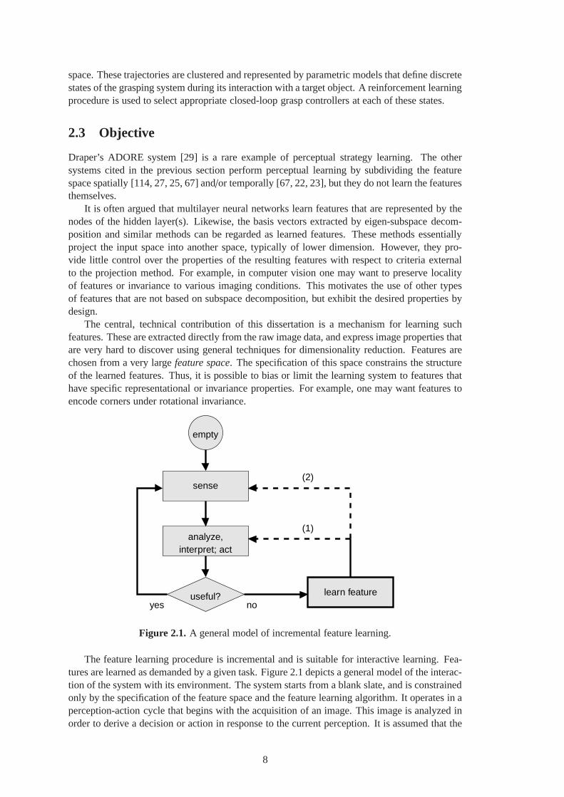
Draper’s ADORE system [29] is a rare example of perceptual strategy learning. The othersystems cited in the previous section perform perceptual learning by subdividing the featurespace spatially [114, 27, 25, 67] and/or temporally [67, 22, 23], but they do not learn the featuresthemselves.

It is often argued that multilayer neural networks learn features that are represented by thenodes of the hidden layer(s). Likewise, the basis vectors extracted by eigen-subspace decom-position and similar methods can be regarded as learned features. These methods essentiallyproject the input space into another space, typically of lower dimension. However, they pro-vide little control over the properties of the resulting features with respect to criteria externalto the projection method. For example, in computer vision one may want to preserve localityof features or invariance to various imaging conditions. This motivates the use of other typesof features that are not based on subspace decomposition, but exhibit the desired properties bydesign.

The central, technical contribution of this dissertation is a mechanism for learning suchfeatures. These are extracted directly from the raw image data, and express image properties thatare very hard to discover using general techniques for dimensionality reduction. Features arechosen from a very largefeature space. The specification of this space constrains the structureof the learned features. Thus, it is possible to bias or limitthe learning system to features thathave specific representational or invariance properties. For example, one may want features toencode corners under rotational invariance.

sense

analyze,interpret; act

useful?yes no

learn feature

empty

(2)

(1)

Figure 2.1. A general model of incremental feature learning.

The feature learning procedure is incremental and is suitable for interactive learning. Fea-tures are learned as demanded by a given task. Figure 2.1 depicts a general model of the interac-tion of the system with its environment. The system starts from a blank slate, and is constrainedonly by the specification of the feature space and the featurelearning algorithm. It operates in aperception-action cycle that begins with the acquisition of an image. This image is analyzed inorder to derive a decision or action in response to the current perception. It is assumed that the

8

system can observe the quality or usefulness of this decision or action. If this response revealsthe adequacy of the action, the agent proceeds with the next perception-action loop. Otherwise,one or more new features are generated with the goal of findingone that will result in superiorfuture actions. The dashed lines designate two alternativeways of operation:

1. If the features can be evaluated immediately without changing the environment, then theagent can iterate feature learning and decision making until a suitable feature has beenfound. The recognition system described in Chapter 4 operates in this way. When thesystem misrecognizes an image, new candidate features are generated one at a time, andare evaluated immediately by rerunning the recognition procedure on the same image.This is indicated by the lower dashed line in Figure 2.1.

2. If a feature cannot be evaluated immediately, then the agent proceeds with the nextperception-action loop. In this case, the generated features are evaluated over time. In thegrasping application (Chapter 6), immediate feature evaluation would require regraspingof an object. To avoid this interference with the task context, after generating new candi-date features the system instead proceeds with the next object, as indicated by the upperdashed line. Evaluation of the newly sampled candidate features is distributed over manyfuture grasps.

These two applications differ significantly not only in their learning mechanisms, but also intheir learning objectives. The recognition application isa supervised classification task. Theutility of a feature is immediately assessed in terms of its contribution to the classification pro-cedures. In contrast, the grasping application is primarily a regression task, where features arelearned that predict a category-specific angular parameter. The utility of a feature depends onits contribution to the value of future behavior of the robot. Training is grounded in the robot’sinteraction with the grasped object, and does not involve anexternal supervisor. Nonetheless,both of these applications employ the same feature space, introduced in the following chapter,and their feature learning algorithms are based on the same basic principles. These differencesand similarities are summarized in Table 2.1.

Table 2.1. Summary of important characteristics of the two applications discussed in this dis-sertation.

Recognition (Ch. 4) Grasping (Ch. 6)classification regressionexternal supervisor learning grounded in interactionimmediate feature evaluation features evaluated over time

same feature spacesame principles for feature learning

All learning algorithms presented in the following chapters are designed to operate incre-mentally. They are very uncommitted to any specific task, andmake few assumptions aboutthe task environment. For example, the recognition algorithm does not know how many knownobject categories – if any – are present in any given scene. This is in contrast to most existingrecognition algorithms that always assign one (or no) classlabel to each scene. Also, neitherapplication has any prior knowledge about the number or nature of the categories to be learned.In short, the algorithms do not assume aclosed world, which has many implications on theirdesign. A consistent set of learning algorithms foropendomains constitute the second keycontribution of this dissertation.

9

2.4 Motivation

In addition to the objectives stated in the preceding section, there are additional, somewhat lesstangible biases and motivations that influenced the design of the representations and algorithmspresented in the following chapters. These are introduced briefly here.

The primary goal of this dissertation is to contribute to ourunderstanding of mechanismsof perceptual learning in humans that can be applied in machine vision systems. Many of theideas manifested in this work are motivated by insights fromperceptual psychology. At theoutset, I believe that humans (children and adults) learn visual features as demanded by tasksthey encounter. Above I presented evidence collected by Schyns and others in support of thisbelief. A subgoal of this work is to contribute to our understanding of human vision, by devisingplausible computational models that describe certain aspects of human vision. I firmly believethat we can learn a great deal from biology for the purpose of advancing technology in theservice of human interests. Specifically, I believe that task-driven, on-line, incremental visuallearning is essential for building sophisticated applied vision systems that operate in general,uncontrolled environments.

With this long-term objective in mind, the mechanisms contributed are applicable in scenar-ios where no external supervisor is available. While the basic learning framework is supervised,the supervisory signal can be produced by the agent itself. In subsequent chapters, I will showhow this can be done.

The construction of the algorithms and the prototype implementation involved a numberof design choices, many of them concerning inessential details. Wherever reasonable, choiceswere made to emulate biological vision. Some of the resulting algorithms are very efficientlyimplemented on massively parallel neural hardware, but arequite expensive when run on aconventional serial computer.

10

CHAPTER 3

AN UNBOUNDED FEATURE SPACE

The necessity for a very large feature space has been motivated briefly above. This chapterintroduces a particular feature space suitable for the objectives of this work.

3.1 Related Work

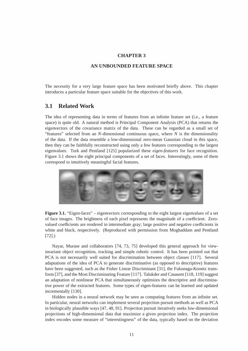
The idea of representing data in terms of features from an infinite feature set (i.e., a featurespace) is quite old. A natural method is Principal ComponentAnalysis (PCA) that returns theeigenvectors of the covariance matrix of the data. These canbe regarded as a small set of“features” selected from anN-dimensional continuous space, whereN is the dimensionalityof the data. If the data resemble a low-dimensional zero-mean Gaussian cloud in this space,then they can be faithfully reconstructed using only a few features corresponding to the largesteigenvalues. Turk and Pentland [125] popularized theseeigen-featuresfor face recognition.Figure 3.1 shows the eight principal components of a set of faces. Interestingly, some of themcorrespond to intuitively meaningful facial features.

Figure 3.1. “Eigen-faces” – eigenvectors corresponding to the eight largest eigenvalues of a setof face images. The brightness of each pixel represents the magnitude of a coefficient. Zero-valued coefficients are rendered in intermediate gray; large positive and negative coefficients inwhite and black, respectively. (Reproduced with permission from Moghaddam and Pentland[72].)

Nayar, Murase and collaborators [74, 73, 75] developed thisgeneral approach for view-invariant object recognition, tracking and simple roboticcontrol. It has been pointed out thatPCA is not necessarily well suited for discrimination between object classes [117]. Severaladaptations of the idea of PCA to generate discriminative (as opposed to descriptive) featureshave been suggested, such as the Fisher Linear Discriminant[31], the Fukunaga-Koontz trans-form [37], and the Most Discriminating Feature [117]. Talukder and Casasent [118, 119] suggestan adaptation of nonlinear PCA that simultaneously optimizes the descriptive and discrimina-tive power of the extracted features. Some types of eigen-features can be learned and updatedincrementally [130].

Hidden nodes in a neural network may be seen as computing features from an infinite set.In particular, neural networks can implement several projection pursuit methods as well as PCAin biologically plausible ways [47, 48, 91]. Projection pursuit iteratively seeks low-dimensionalprojections of high-dimensional data that maximize a givenprojection index. The projectionindex encodes some measure of “interestingness” of the data, typically based on the deviation

11

from Gaussian normality [59, 36, 99]. The projections generated by a projection index based onsecond-order statistics correspond to the principal components of the data.

All of these methods, with the exception of certain types of neural networks, computeglobalfeatures. In contrast, it is often desirable to producelocal features that represent spatially local-ized image characteristics. Localized variants of eigen-features have been explored [26].

A variety of local features have been proposed in the contextof recognition systems. In atypical approach, a feature is a vector of responses to a set of locally applied basis filter kernels.Koenderink [57] suggests that the neighborhood around an image point can be represented bya set of Gaussian derivatives of various orders, termed alocal jet, derived from a local Taylorseries expansion of the image intensity surface. Some related schemes are based on steerablebases of Gaussian-derivative filters [90, 104, 94, 43], which will be briefly discussed in Section3.3.2. Others employ Gabor filters [128, 20], curved variants known asbanana wavelets[58],or Haar wavelets [81] to represent local appearance.

A different way to generate an unbounded feature space is by defining a feature as a param-eterized composition of several components. Cho and Dunn [18] define a corner feature by thedistance and angle between two straight line segments. Their feature set is finite because theseparameters are quantized.

Segen [110] was one of the first to consider an infinite combinatorial feature space in acomputer vision context. His shape recognition system is based on structural compounds oflocal features. Geometric relations between local curvature descriptors are represented by amultilevel graph, and concept models of 2-D shapes are constructed by matching and mergingmultiple instances of such graphs. Califano and Mohan [16] combined triplets of local cur-vature descriptors to form a multidimensional index used for recognition of 2-D shapes. Theircontributions include a quantitative probabilistic argument demonstrating that the discriminativepower of features increases with their degrees of freedom.

Amit, Geman and their coworkers create a potentially infinite variety of features from aquantized space by means of combinatorics. Primitive localfeatures are composed to produceincreasingly complex arrangements. Primitive features are defined by co-occurrences of smallnumbers of binarized pixel values, and compounds are characterized by relaxed geometric rela-tionships. Discriminative features are constructed and queried efficiently using a decision treeprocedure. This type of approach has been applied to handwritten character recognition [8, 5]and face detection [7, 6] with remarkable success, and has also been extended to recognition ofthree-dimensional objects [50]. The approach employed in this dissertation borrows and extendskey ideas from this work.

3.2 Objective

The representational power of any system that uses featuresto represent concepts is determinedto a large extent by the available features. If the feature set is not sufficiently expressive forthe task at hand, the performance of the system will be limited forever. If the feature set istoo expressive, the system will be prone to a variety of problems, including overfitting, and tobiases introduced through pairwise correlated features ordistractor features that do not correlatewell with important distinctions. Clearly, different features may be relevant for different tasks.Moreover, given a task, different feature sets may be suitable for different algorithms employedto solve the same task [52].

These considerations require that features either be hand-crafted for a particular setting (con-sisting of task, algorithm and data), or that they be learnedby the system. This chapter definesa feature space for use with a feature learning system, subject to the following objectives:

1. As this work is concerned with visual tasks, features are computed on intensity images.

12

2. The feature space should not be geared toward any task, butit should contain features thatare suitable for a variety of visual tasks at various levels of specificity and generality. Inother words, there should be some features that are highly useful for any of a variety oftasks that the system may be asked to solve.

3. Since the characteristics of a feature learning system are best demonstrated on a systemthat learns few but powerful features, the feature space should contain features that areindividually very useful for given tasks. This is in contrast to most existing feature-basedvision systems that derive their power primarily from a large numberof features that arenot necessarily very powerful individually.

4. The feature space should be sufficiently complete to demonstrate success on exampletasks using feature learning systems discussed in subsequent chapters.

5. Since image-plane orientation is important in some tasksand irrelevant in others, fea-tures should inherently allow the measurement of feature orientation in a way that can beexploited to achieve normalization for rotation.

6. Since in many visual tasks there is no prior scale information available, features shouldbe robust to variations in scale to simplify computation.

7. To enhance robustness to clutter and occlusion and to facilitate the learning of categoriescharacterized by unique object parts, features should be local in the image array.

8. For generality, features should be applicable in generalclassification and regression frame-works.

9. The features should be a plausible functional model of relevant aspects of the humanvisual system.1

All of the methods discussed in the preceding section satisfy some of these objectives, butnone of them satisfies all. Eigen-features and their variations are well suited for a variety oftasks, but rotational invariance and image-plane localityare hard to achieve. Wavelets and Ga-bor filters and their variants are local, but are not rotationally invariant. Filters based on steer-able Gaussian-derivative filters satisfy all of the above objectives. The steerability property, tobe explained in Section 3.3.2, allows the synthesis of filters and their responses at arbitrary ori-entations from a small set of basis filters, and can be exploited to achieve rotational invarianceat very little computational cost. However, the representational and distinctive power of indi-vidual, well-localized (Objective 7) Gaussian-derivative filters is not sufficient for many tasks(Objective 3). Amit and Geman [8, 5] used relatively weak individual features, sparse binarypixel templates, and showed how to increase their power by composing them in a combinatorialfashion.

The key idea to achieving all of the above objectives is to combine steerable Gaussian-derivative filters with an adaptation of Amit and Geman’s idea, producing features that consistof spatial combinations of local appearance characteristics. Before the details are presented, thefollowing section provides some helpful background.

3.3 Background

This section presents brief introductions to relevant concepts that have been well established inthe literature. Some familiarity with these concepts is required to understand the contributionspresented in subsequent sections.

1Since this contradicts Objective 5, rotational (non-)invariance is not considered a relevant aspect here.

13

3.3.1 Gaussian-Derivative Filters

The isotropic zero-mean Gaussian function with varianceσ2 of a two-dimensional parameterspace at a pointx = [x, y]T ∈ R2 is defined as

G(x, σ) =1

2πσ2e−

xT x2σ2 . (3.1)

For the purposes of this work, the oriented derivative of a Gaussian of orderd at orientationθ = 0, i.e. in thex direction, is written as

G0d(x, σ) =

∂d

∂dxG(x, σ). (3.2)

For general orientationsθ, Gθd is defined as an appropriately rotated version ofG0d(x, σ), i.e.

Gθd(x, σ) = G0d(Rθx, σ) (3.3)

with a rotation matrix

Rθ =

[

cosθ − sinθsinθ cosθ

]

.

Gaussian-derivative filter kernels are discrete versions of Gaussian point spread functionscomputed in this way. To generate a filtered versionIG(x) of an imageI (x), a discrete convo-lution with a kernelG is performed. Two-dimensional convolutions with Gaussians and theirderivatives can be computed very efficiently because the kernels are separable, and highly accu-rate and efficient recursive approximations exist [127]. Unfortunately, this is not generally trueof rotated derivatives (Equation 3.3).

Gaussian G0

First derivative G01 Gπ/21

Second derivative G02 Gπ/32 G2π/3

2

Figure 3.2.Visualization of a two-dimensional Gaussian function and some oriented derivatives(cf. Equation 3.3). Zero values are shown as intermediate gray, positive values are lighter,negative values darker.

Figure 3.2 illustrates some oriented Gaussian-derivativefilters used in the context of thiswork. Gaussian filters act as low-pass filters, and their derivatives as bandpass filters. Thecenter frequency increases (see Figure 3.2) and the bandwidth decreases as the order of thederivative increases. First-order derivative kernels respond to intensity gradients inI . To extractedge information from an imageI , I is convolved with the two orthogonal basis filtersG0

1 and

Gπ/21 . The gradient magnitudes and orientations inI are then easily computed:

|∇I | =√

I2G0

1

+ I2Gπ/21

(3.4)

14

tanθ∇I = IGπ/21/ IG0

1(3.5)

When computingθ∇I using Equation 3.5, the full angular range of 0–2π can be recovered by tak-ing into account the signs of the numerator and the denominator when computing the arctangent.For a thorough discussion of Gaussian-derivative filters see a recent book chapter [93].

3.3.2 Steerable Filters

A class of filters issteerableif a filter of a particular orientation can be synthesized as alinearcombination of a set ofbasis filters[35]. For example, first-order Gaussian-derivative filtersaresteerable, since

Gθ1 = G01 cosθ +Gπ/21 sinθ (3.6)

as is easily verified. Due to the linearity of the convolutionoperation, an image filtered at anyorientation can be computed from the corresponding basis images:

IGθ1 = IG01cosθ + IGπ/21

sinθ (3.7)

which is much more efficiently computed for many different values ofθ than by explicit convo-lution with the individual filtersGθ1.

Gaussian-derivative filters of any orderd are steerable usingd + 1 basis filtersGθk,dd that areequally spaced in orientation between 0 andπ, i.e.,

θk,d =kπ

d + 1, k = 0, . . . , d.

Incidentally, Figure 3.2 shows the basis filtersGθk,dd for the first two derivatives. To synthesize afilter at any given orientationθ, these basis filters are combined using the rule

Gθd =d

∑

k=0

Gθk,dd cθk,d (3.8)

wherecθk,1 = cos(θ − kπ/2) k = 0, 1

cθk,2 = 13

(

1+ 2 cos(2(θ − kπ/3)))

k = 0, 1, 2

cθk,3 = 12

(

cos(θ − kπ/4)+ cos(3(θ − kπ/4)))

k = 0, 1, 2, 3

which contains Equation 3.6 as a particular case [35, 90]. Again, due to the linearity of con-volution, the same operation can be performed on the filteredimages, as opposed to the filtersthemselves. See Freeman and Adelson [35] for a thorough treatment of steerable filters.

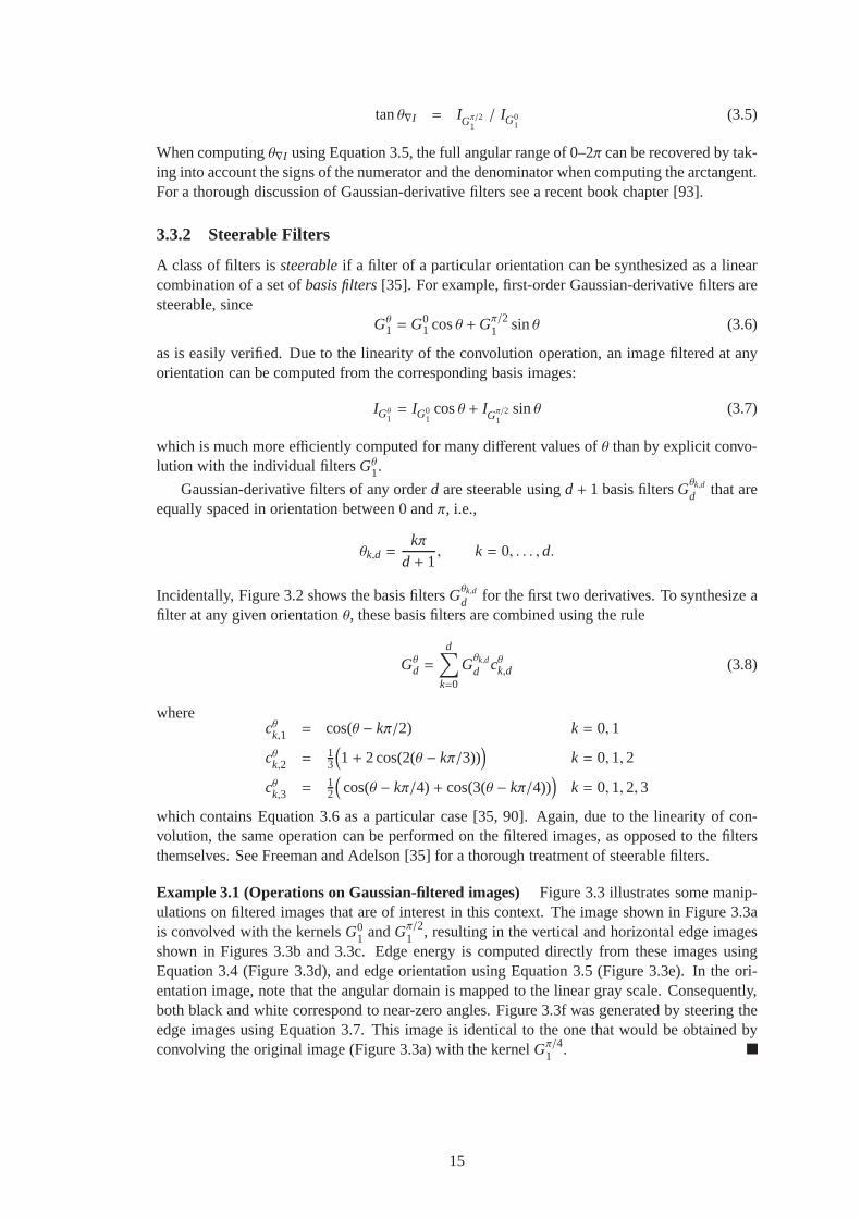
Example 3.1 (Operations on Gaussian-filtered images) Figure 3.3 illustrates some manip-ulations on filtered images that are of interest in this context. The image shown in Figure 3.3ais convolved with the kernelsG0

1 andGπ/21 , resulting in the vertical and horizontal edge imagesshown in Figures 3.3b and 3.3c. Edge energy is computed directly from these images usingEquation 3.4 (Figure 3.3d), and edge orientation using Equation 3.5 (Figure 3.3e). In the ori-entation image, note that the angular domain is mapped to thelinear gray scale. Consequently,both black and white correspond to near-zero angles. Figure3.3f was generated by steering theedge images using Equation 3.7. This image is identical to the one that would be obtained byconvolving the original image (Figure 3.3a) with the kernelGπ/41 .

15

(a) (b) (c) (d) (e) (f)

I IG01

IGπ/21

√

I2G0

1

+ I2Gπ/21

tan−1IGπ/21IG0

1

IG01cosπ4

+ IGπ/21sin π4

Figure 3.3. Example manipulations with first-derivative images. Imagea shows the originalimage of size 128× 128 pixels. In images b, c, and f, zero values are encoded as intermediategray, and positive and negative values as lighter and darkershades, respectively. In image d,black represents zero. In image e, the angular range of 0–2π is mapped to the range from blackto white. The derivatives were computed withσ = 2 pixels. See Example 3.1 for discussion.

3.3.3 Scale-Space Theory

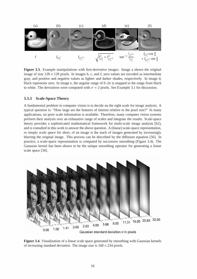
A fundamental problem in computer vision is to decide on the right scale for image analysis. Atypical question is: “How large are the features of interestrelative to the pixel size?” In manyapplications, no prior scale information is available. Therefore, many computer vision systemsperform their analysis over an exhaustive range of scales and integrate the results. Scale-spacetheory provides a sophisticated mathematical framework for multi-scale image analysis [62],and is consulted in this work to answer the above question. A (linear) scale-space representation,or simply scale spacefor short, of an image is the stack of images generated by increasinglyblurring the original image. This process can be described by the diffusion equation [56]. Inpractice, a scale-space representation is computed by successive smoothing (Figure 3.4). TheGaussian kernel has been shown to be the unique smoothing operator for generating a linearscale space [34].

Figure 3.4. Visualization of a linear scale space generated by smoothing with Gaussian kernelsof increasing standard deviation. The image size is 168× 234 pixels.

16

For the purposes of this work, scale-space theory offers well-motivated ways to identifyappropriate scales for image analysis at each location in animage, based on the followingscale-selection principle:

“In the absence of other evidence, assume that a scale level,at which some (pos-sibly non-linear) combination of normalized derivatives assumes a local maximumover scales, can be treated as reflecting a characteristic length of a correspondingstructure in the data.” [64]

Lindeberg [64] provides some theoretical justification forthis principle derived from the obser-vation that if an image is rescaled by a constant factor, thenthe scale at which a combinationof normalized derivatives assumes a maximum is multiplied by the same factor. The choiceof a specific combination of normalized derivatives – in the following denoted ascale functions(σ) – depends on the type of image structure of interest. Such structures and their associatedscales can then be detected simultaneously in an image by finding local maxima ofs in the scalespace. Thus, there are typically multipleintrinsic scalesassociated with each image location.The normalization is done with respect to the operator scaleσ, and ensures that the values ofthe scale function can be compared across scales.

Figure 3.5. Example of a scale functions(σ). The graph shows the scale function computed for13 discrete values ofσ at the center pixel of the image (121×121 pixels). Each local maximumdefines an intrinsic scale at this point. The two intrinsic scales are illustrated by circles ofcorresponding radii.

Example 3.2 (Intrinsic Scale) Figure 3.5 illustrates the computation of the intrinsic scalesat an image location. The graph plots the values ofs(σ) at this point, computed for discretevalues ofσ at half-octave spacing. The local maxima of this graph definethe intrinsic scales,which are illustrated by circles of corresponding radii in the image. The stronger maximum(s(5.7) = 73.6) captures the size of the dark, solid region at the center ofthe sunflower, whilethe weaker maximum (s(22.6) = 7.1) roughly corresponds to the size of the entire flower. Themaximum at the minimal value ofσ = 1 is not considered a scale-space maximum because it isnot enclosed between lower values ofs.

To illustrate hows(σ) can be used to detect image structures of interest at their intrinsic scale,Figure 3.6 shows the 200 strongest local maxima of the same scale functions(σ) computedeverywhere in the image. To generate this figure, the value ofs(σ) was computed at eachpixel for each value ofσ. The corresponding local maxima within the resulting scalespace areillustrated by circles of the corresponding radiusσ at the corresponding locationx. The figureclearly illustrates the correspondence of intrinsic scalewith the size of local image structures,which is here dominated by sunflowers. The scale found for thelarge sunflower at the lowerright is smaller than expected because no larger scales wereconsidered at this point to avoid

17

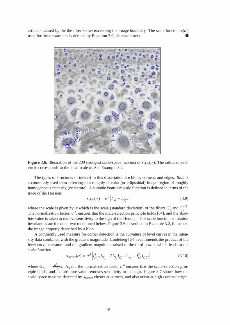
artifacts caused by the the filter kernel exceeding the imageboundary. The scale functions(σ)used for these examples is defined by Equation 3.9, discussednext.

Figure 3.6. Illustration of the 200 strongest scale-space maxima ofsblob(σ). The radius of eachcircle corresponds to the local scaleσ. See Example 3.2.

The types of structures of interest in this dissertation areblobs, corners, and edges.Blob isa commonly used term referring to a roughly circular (or ellipsoidal) image region of roughlyhomogeneous intensity (or texture). A suitable isotropic scale function is defined in terms of thetrace of the Hessian:

sblob(σ) = σ2∣

∣

∣

∣

IG02+ IGπ/22

∣

∣

∣

∣

(3.9)

where the scale is given byσ which is the scale (standard deviation) of the filtersG02 andGπ/22 .

The normalization factor,σ2, ensures that the scale-selection principle holds [64], and the abso-lute value is taken to remove sensitivity to the sign of the Hessian. This scale function is rotationinvariant as are the other two mentioned below. Figure 3.6, described in Example 3.2, illustratesthe image property described by a blob.

A commonly used measure for corner detection is the curvature of level curves in the inten-sity data combined with the gradient magnitude. Lindeberg [64] recommends the product of thelevel curve curvature and the gradient magnitude raised to the third power, which leads to thescale function

scorner(σ) = σ4∣

∣

∣

∣

∣

I2Gπ/21

IG02− 2IG0

1IGπ/21

IGx,y + I2G0

1IGπ/22

∣

∣

∣

∣

∣

(3.10)

whereGx,y =∂2

∂x∂yG. Again, the normalization factorσ4 ensures that the scale-selection prin-ciple holds, and the absolute value removes sensitivity to the sign. Figure 3.7 shows how thescale-space maxima detected byscornercluster at corners, and also occur at high-contrast edges.

18

Figure 3.7. Illustration of scale-space maxima ofscorner(σ). The left image shows the strongest15 scale-space maxima, and the right image the strongest 80.The radius of each circle corre-sponds to the local scaleσ.

For intensity edges, a useful scale function is based on the first spatial derivative [63]:

sedge(σ) =

√

σ

(

I2G0

1

+ I2Gπ/21

)

(3.11)

The normalization factor√σ ensures the scale-selection principle as before. The normalization

factors for blobs and corners as formulated above are chosensuch that the recovered scalescorrespond to the size of the local image structure, and willthus typically be related to thesize of objects depicted in the image. In contrast, the normalization factor for edges is chosento reflect the sharpness of the edge. Sharp edges attain theirscale-space maxima at smallerscales than blurry edges. For the purposes of this dissertation, the reason for this choice of scalenormalization is that it ensures perfect localization of the recovered edges at the maxima in thegradient magnitude along the gradient direction.

As noted above, blob and corner features are identified as local maxima of the scale functionin the scale space. To extract edges in scale space, gradient-parallel maxima are extracted fromthe scale space according to the notion of non-maximum suppression [17]. This results in thinand mostly contiguous edges. Since the details of scale-space edge extraction are unimportantin the context of this work, the interested reader is referred to the literature [63].

3.4 Primitive Features

Sections 3.1 and 3.2 discussed important properties and various ways to generate global andlocal features. Since eigen-features have a number of desirable properties, it is worth consid-ering how their primary drawback – their global spatial extent – can be overcome. Colin deVerdiere and Crowley investigated this question and developed a recognition system based onlocal descriptors derived by PCA [26]. Many of the most important eigen-features generatedby their system resemble oriented bandpass filters. This is no accident: If natural images aredecomposed into linearly independent (but not necessarilyorthogonal) basis functions, using asparseness or minimum-description-length objective thatfavors representations with many van-ishing coefficients, then basis functions emerge that resemble orientedbandpass filters. Notably,these are stronglylocalized– even without an explicit constraint or bias toward locality [80, 91].This result has been well established in the literature, andserves as a natural explanation for the

19

shape of receptive fields in the mammalian early visual pathway. The receptive fields of vi-sual neurons in the primary visual cortex have often been modeled by oriented derivatives ofGaussian functions [132, 57].

In this dissertation, these insights motivate the choice ofGaussian-derivative filters as afundamental representation of local appearance. Since principled and biologically plausiblefeature extraction mechanisms tend to result in features resembling Gaussian derivatives, theyare used here directly, avoiding the added effort of eigen-subspace decomposition. Moreover,Gaussians and their derivatives have a number of useful properties; those that are important forthis work were introduced in Section 3.3.

The feature space considered in this work is defined recursively: A feature from this space iseither aprimitive feature, or acompoundfeature. Compound features consist of other compoundfeatures and/or primitive features, and are discussed in Section 3.5. A primitive feature is definedby a vector of responses of Gaussian-derivative filters all computed at the same image locationx. The following sections describe two types of primitive features.

3.4.1 Edgels

Edges are a fundamental concept in vision, deemed importantby both machine and biologicalvision research. Edges describe aspects of shape in terms ofintensity boundaries. Here, indi-vidual edge elements – so-callededgels– are considered in isolation, without attempting to jointhem into contours. An edgel is defined by the 2-vector

fedgel(x) =

IG01(x)

IGπ/21(x)

where the filtersG are computed at theintrinsic scaleσx that maximizessedgel(σ) at the imagelocationx. An edgel encodes the orientation and magnitude of the localintensity gradient at theintrinsic scale. Note that the gradient orientation is always numerically stable at a scale-spacemaximum, because the numerator and denominator in Equation3.5 cannot both be close to zeroat a maximum of the scale functionsedgel.

3.4.2 Texels

Edgels are a weak descriptor of the local intensity surface in that they are defined by merely twoparameters. It may often be desirable to have a more expressive local descriptor that uses moreparameters and captures more structure than just the local intensity gradient. Intuitively, thisstructure corresponds to a local pattern or texture, which motivates the termtexel (for textureelement). A texelftexel is defined by a vector containing the steerable bases of the first nd

Gaussian derivatives atns scales. One of these scales is the intrinsic scaleσ that maximizessblob(σ) or scorner(σ) at an image location.

Besides the choice of the scale function, an edgel is simply atexel withnd = ns = 1. Themotivation for using texels with several derivatives and scales is that the additional parametersrepresent more information about local image structure (ortexture), increasing the specificityof the feature [90]. This increased specificity may or may notbe desirable in a given task.Therefore, both edgels and texels are included in the feature space, and it is up to the featurelearning algorithms (Chapters 4 and 6) to use any or both of these primitive feature types.

This work consistently uses texels composed of the first two derivatives at three scales,yielding a total of (2+ 3)× 3 = 15 filter responses. The middle scale is the intrinsic scale at thatimage location, and the other two scales are spaced half an octave below and above. Derivativesof an order greater than about two or three rarely respond significantly in practice because oftheir narrow bandpass characteristics. Therefore, they contribute little to the specificity of afeature. The specificity can arbitrarily be increased by adding scales (within the limits imposed

20

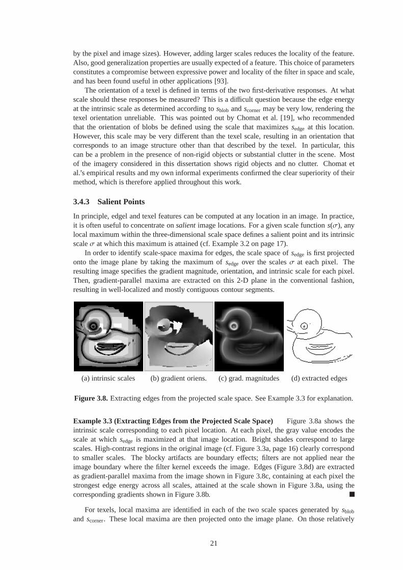
by the pixel and image sizes). However, adding larger scalesreduces the locality of the feature.Also, good generalization properties are usually expectedof a feature. This choice of parametersconstitutes a compromise between expressive power and locality of the filter in space and scale,and has been found useful in other applications [93].

The orientation of a texel is defined in terms of the two first-derivative responses. At whatscale should these responses be measured? This is a difficult question because the edge energyat the intrinsic scale as determined according tosblob andscornermay be very low, rendering thetexel orientation unreliable. This was pointed out by Chomat et al. [19], who recommendedthat the orientation of blobs be defined using the scale that maximizessedge at this location.However, this scale may be very different than the texel scale, resulting in an orientation thatcorresponds to an image structure other than that describedby the texel. In particular, thiscan be a problem in the presence of non-rigid objects or substantial clutter in the scene. Mostof the imagery considered in this dissertation shows rigid objects and no clutter. Chomat etal.’s empirical results and my own informal experiments confirmed the clear superiority of theirmethod, which is therefore applied throughout this work.

3.4.3 Salient Points

In principle, edgel and texel features can be computed at anylocation in an image. In practice,it is often useful to concentrate onsalient image locations. For a given scale functions(σ), anylocal maximum within the three-dimensional scale space defines a salient point and its intrinsicscaleσ at which this maximum is attained (cf. Example 3.2 on page 17).

In order to identify scale-space maxima for edges, the scalespace ofsedge is first projectedonto the image plane by taking the maximum ofsedge over the scalesσ at each pixel. Theresulting image specifies the gradient magnitude, orientation, and intrinsic scale for each pixel.Then, gradient-parallel maxima are extracted on this 2-D plane in the conventional fashion,resulting in well-localized and mostly contiguous contoursegments.

(a) intrinsic scales (b) gradient oriens. (c) grad. magnitudes (d) extracted edges

Figure 3.8. Extracting edges from the projected scale space. See Example 3.3 for explanation.

Example 3.3 (Extracting Edges from the Projected Scale Space) Figure 3.8a shows theintrinsic scale corresponding to each pixel location. At each pixel, the gray value encodes thescale at whichsedge is maximized at that image location. Bright shades correspond to largescales. High-contrast regions in the original image (cf. Figure 3.3a, page 16) clearly correspondto smaller scales. The blocky artifacts are boundary effects; filters are not applied near theimage boundary where the filter kernel exceeds the image. Edges (Figure 3.8d) are extractedas gradient-parallel maxima from the image shown in Figure 3.8c, containing at each pixel thestrongest edge energy across all scales, attained at the scale shown in Figure 3.8a, using thecorresponding gradients shown in Figure 3.8b.

For texels, local maxima are identified in each of the two scale spaces generated bysblob

and scorner. These local maxima are then projected onto the image plane.On those relatively

21

rare occasions where two local maxima project to the same image location, the maximum cor-responding to the larger scale is shifted slightly. The set of salient texel points is then given bythe union of the projected maxima of both scale spaces. As a result, each salient image pointhas exactly one intrinsic scale (Figure 3.9).

689 edgels 130 texels (54 blobs, 76 corners)

430 edgels 77 texels (30 blobs, 47 corners)

Figure 3.9. Salient edgels and texels extracted from an example image. On the left, eachdark line segment corresponds to an edgel (i.e., a scale-space maximum ofsedge) located atthe midpoint of the line, with scaleσ identical to half the length of the line. On the right,square markers correspond to scale-space maxima ofscorner, and circular markers to scale-spacemaxima ofsblob. Collectively, these are the salient texels. The orientations of these are illustratedby the center lines of each marker. The radius of each marker is equal to the local scaleσ. SeeExample 3.4 for discussion.

Scale spaces are computed at half-octave spacing, i.e.,σi+1 = σi√

2. This choice providessufficient resolution at moderate computational cost [93]. The minimum plausible scale is re-lated to the pixel size, and the maximum is limited by the sizeof the image. This work usesscales in the range between one pixel and one quarter of the lesser image dimension.

Example 3.4 (Salient Edgels and Texels) Figure 3.9 illustrates the salient edgels and texelsextracted from an example image. The radius of each edgel andtexel marker shown in the figure

22

is equal to the local scaleσ. Circles and squares correspond to blobs and corners, respectively.The bottom row illustrates the degree of robustness of the salient points with respect to rotationand scale. These images were obtained by rotating the original duck image by 60 degrees andscaling it by a factor of 0.7 and subsampling, but are shown enlarged to match the original size tofacilitate visual comparison. Naturally, some amount of detail is lost through the subsampling,which accounts for the reduced number of salient points.

Most edgels are located at high-contrast image locations and are extracted at a very small scale.In addition, some edgels were extracted at much larger scales, capturing large-scale image struc-tures as opposed to pixel-level localized gradients. Likewise, texels cluster around high-contrastimage regions. While edgel scales reflect the smoothness of the local edge, texel scales corre-spond to the size of the image structure. Note, for example, the large corner behind the neck, orthe small blob at the tip of the tail. All of these are located at local maxima in the scale function;there was no threshold on the prominence of these local maxima. Many of the weaker max-ima tend to occur in clusters along intensity edges, especially at smaller scales. As the figureillustrates, such texels are less robust to image transformations than texels at more pronouncedlocations, e.g. the blob centered at the eye, the large corner behind the neck, the small blob atthe tip of the tail, or the blob at the chest underneath the chin.

Figure 3.10 illustrates the extent to which texels are stable across viewpoint changes. Again,those texels that correspond to pronounced locations tend to be more stable. Texels locatedat accidental maxima along intensity edges are reliably present, but their precise number andlocation varies across viewpoints.

Figure 3.10. Stability of texels across viewpoints. Adjacent viewpoints differ by 10 degrees.See Example 3.4 for discussion.

23

3.4.4 Feature Responses and the Value of a Feature

As introduced in Sections 3.4.1 and 3.4.2, a specific instance f (p) of a primitive feature is de-fined by the numerical values comprising the feature response vector, typically generated bycomputing the applicable filter responses at a locationp in some image. To find occurrences off (p) in an imageI , the response strength orvalue ff (p)(x) of f (p) is measured at each pointxin I . To measure the feature value at a locationx, the feature response vectorf (x) is computedat x, using the local intrinsic scaleσx. The feature value is then given by the normalized innerproduct of the observed responsef (x) with the reference responsef (p):

ff (p)(x) = max

{

0,f (p)T f (x)‖f (p)‖ ‖f (x)‖

}

(3.12)

Negative values are considered as weak as orthogonal response vectors, and are therefore cutoff at zero. Hence, 0≤ ff ≤ 1. The normalized inner product is pleasing in that it returns thecosine of the angle between the vectors in question which, for edgels, is identical to the cosineof the angle between the edgels in the image plane:ff (p)(x) = max{0, cos(θp − θx)}. Moreover,the feature value is invariant to linear changes in image intensity.

If the feature value is to be computed regardless of the orientation of a feature in the imageplane, the measured feature response vectorf (x) is first steered to match the orientation of thepattern vectorf (p) before Equation 3.12 is applied. This is done using a function f (x, p) thatapplies the steering equation (3.8, page 15) to all components of f (x), usingθ = θp − θx. Thus,Equation 3.12 becomes

ff (p)(x) = max

0,f (p)T f (x, p)

‖f (p)‖∥

∥

∥f (x, p)∥

∥

∥

(3.13)

for rotationally invariant feature value computation. Note that this rotationally-invariant match-ing implies that ff is always equal to one iff is an edgel. Hence, individual edgels carry noinformation. Rotation-invariant edgels are only useful aspart of a compound feature, as intro-duced in the following section.

(a) f (p) (b) f (x∗) (c) f (x∗t )

Figure 3.11. Matching a texel (a) across rotation and scale, without (b) and with (c) rotationalnormalization. See Example 3.5 for explanation.

Example 3.5 (Localizing a Feature) Figure 3.11a shows one of the salient texels extractedfrom the familiar duck image (cf. Figure 3.9). Figures 3.11band 3.11c show the same rotatedand scaled version as used in Figure 3.9. Letp = [71, 49]T , which is the location of the texelshown in Figure 3.11a. Then,f (p) is the feature response vector defining this texel feature.Wenow want to find this feature in the rotated and scaled image. To do this without regard to featureorientation, the locationx∗ that maximizesff (p)(x) is identified using Equation 3.12. The salient

24

point x∗ that maximizes Equation 3.12 is that shown in Figure 3.11b. Here, ff (p)(x∗) = 0.956.It is no accident that this texel has the same orientation as the pattern featuref (p) shown inFigure 3.11a, but the two locations do not correspond (even though they are spatially close toone another in this example). The true corresponding feature is shown in Figure 3.11c; let uscall this locationx∗t . Disregarding the difference in orientation,ff (p)(x∗t ) = 0.578< ff (p)(x∗). Ifat each locationx the feature response vectorf (x) is first steered to match the orientation off (p)using Equation 3.13, then the correct location is found withff (p)(x∗t ) = 0.996 (Figure 3.11c). Incontrast, the value atx∗ increases only marginally fromff (p)(x∗) = 0.956 to ff (p)(x∗) = 0.960,remaining below the value at the correct locationx∗t .

In all parts of this work, feature values are computed with rotational normalization usingEquation 3.13. From now on, the tilde will be omitted for simplicity, and the notationff will beused with the understanding that feature response vectors are always steered to achieve rotationalinvariance.

A featuref (p) is present in an imageI to the degree

ff (p)(I ) = maxx∈I

ff (p)(x). (3.14)

This computation is quite expensive, as it involves the measurement of the intrinsic scale andthe computation off (x) and ff (p)(x) at each location in the image. A large proportion of thiscomputation is going to be wasted because most image regionswill not contain features ofpractical relevance. Therefore, the assumption is made that all features of practical relevance arelocated at salient points. To identify the salient points itis still necessary to evaluates(σ) overthe entire range of scalesσ everywhere in the image, which constitutes a highly parallelizableoperation. Moreover, if the application provides a fixed setof training images, this computationcan be performed off-line. In practice, this leads to a great reduction in computation time andspace, as the maximum in Equation 3.14 is only taken over the salient points rather than theentire image.

3.5 Compound Features

A core objective of this work is to demonstrate that featurescan be learned that are highly mean-ingful individually. The limited descriptive power of individual primitive features is overcomeby composing two or more primitive features into compound features. Since compound fea-tures contain more parameters and cover a larger image area than do primitive features, theyprovide a potentially more specific and robust description of relevant aspects of appearance.What it means for a feature to be relevant, and how relevant features are sought, depends onthe given task. Chapters 4 and 6 present two illustrative examples. This section describes threecomplementary ways in which primitive features can be composed into compound features.

There is evidence that the mammalian visual cortex also composes simple and generic fea-tures hierarchically into more complex and specific features. The primary visual cortex con-tains retinotopic arrays of local and oriented receptive fields [45] which have been modeled asGaussian-derivative functions [132, 57]. Many neurons found in higher-order visual cortices aretuned to more complex stimuli. Riesenhuber and Poggio [96] proposed a hierarchical model ofrecognition in the visual cortex, using spatial combinations of view-tuned units not unlike thecompound features introduced below.

3.5.1 Geometric Composition

The structure of a geometric compound ofnf ≥ 2 primitive featuresf0, f1, . . . , fnf−1 (Figure 3.12)is defined by the attitudesφi of each subfeature, and the angles∆θi , distancesdi , and scale ratios∆σi between the constituent subfeaturesf i . The distancesdi are given relative to the intrinsic

25

scaleσi−1 at pointi − 1. Each primitive feature is either an edgel or a texel. A specific instancefgeomof a geometric feature with a given structure is defined by theconcatenation of the vectorscomprising the primitive subfeatures. Its orientation is denoted byθ, which is the orientation ofthe reference point.

��

��

��

reference pointf0

θ

φ1

d1φ2

d2

f2

f1

Figure 3.12.A geometric compound feature consisting of three primitivefeatures.

The location of a feature is defined by the location of the reference point. To extract thefilter response vector defining a geometric featuref (x) at locationx, the following procedure isused:

Algorithm 3.6 (Extraction of a Geometric-Compound FeatureResponse Vector)

1. The response vectorf0(x) is computed atx. This defines the orientationθx and intrinsicscaleσx of f (x). Initially, let i = 1:

2. If i = nf , then stop.

3. The locationxi , orientationθi , and scalesi of the next constituent subfeaturef i are com-puted:

xi = xi−1 + σi−1di

[

cos(θi−1 + φi)sin(θi−1 + φi)

]

θi = θi−1 + ∆θi

σi = σi−1∆σi

4. The feature response vectorf i(xi) is computed at scaleσi, and is rotated to orientationθiusing the steering equation 3.8 (page 15) with angular argumentθ = ∆θi . Incrementi, andcontinue at step 2.

The filter response vector is given by the concatenation of the individual response vectors of theconstituent primitive featuresf (xi), i = 0, 1, . . . , nf − 1.

The value ffgeom(I ) of a geometric compound featurefgeom in an imageI is computed in thesame way as for a primitive feature (Equations 3.13 and 3.14), using the concatenated responsevectors. This involves running Algorithm 3.6 at each of thensal applicable salient image loca-tions. These are either all salient edgels or all salient texels, depending on the type of the firstsubfeaturef0 of fgeom. It is easily seen that the time required to computeffgeom is proportional tonsalnf .

3.5.2 Boolean Composition

A Boolean compound feature consists of exactly two subfeatures, each of which can be a prim-itive or a compound feature. The relative locations of the subfeatures are unimportant. Twotypes of Boolean features have been defined:

26

• The value of aconjunctivefeature is given by the product of the values of the two subfea-tures.

• The value of adisjunctive feature is given by the maximum of the values of the twosubfeatures.

For conjunctive features, the product is used instead of theminimum because it is natural toassign a higher value to a feature if the larger of the two component values is increased evenfurther. For example, the valueff of a conjunctive feature with subfeature valuesff1 = 0.6 andff2 = 0.9 should be larger than for a feature with subfeature valuesff1 = 0.6 and ff2 = 0.7.

Feature values of Boolean compound features are measured recursively by first measuringthe values of each of the two subfeatures individually, and then combining their values using theproduct or the maximum, respectively. Hence, the time required to compute the valueffbool(I ) ofa Boolean compound featurefbool in an imageI is proportional tonsal,0t0(I ) + nsal,1t1(I ), wherensal,i denotes the number of salient image points applicable to subfeaturef i , andti(I ) denotes thetime required to compute the valueff i (I ) of subfeaturef i in the image. Note that each subfeatureof a Boolean compound feature can be any type of feature, including primitives, or geometric,conjunctive or disjunctive compounds.

3.6 Discussion

Section 3.2 formulated a list of objectives (page 12) to be met by the feature design. All of theseare addressed by the compositional feature space:

1. Features are computed on intensity images.

2. The feature space was designed without a specific task in mind. Features can be composedto arbitrary structural complexity to increase their specificity.

3. Therefore, it seems justified to hope that powerful individual features are contained in thisfeature space. The extent to which this goal was achieved will be discussed in Chapters4–6.

4. Edgels and texels are complementary and capture important aspects of image structure.Geometric and Boolean compositions are also complementaryand have intuitive seman-tics. Subsequent chapters will illustrate possibilities and limitations of this feature spacefor practical tasks.

5. Feature orientations are easily computed and compensated for using the steerability prop-erty of the filters employed.

6. The features are computed at the intrinsic scale observedin the images. Therefore, theyare useful for scale-invariant image analysis.

7. The features are local, since the filters employed have local support. The locality of geo-metric features can be controlled by placing constraints onthe distances between primi-tives and the number of primitives allowed.

8. Features return a scalar value, which makes them applicable in general classification andregression frameworks. The orientation attribute of a feature can also be used for regres-sion, as will be seen in Chapter 6.

9. The biological relevance of this feature space was briefly discussed in the introductionsto Sections 3.4 and 3.5.

27

A critical property of this compositional feature space is that it is partiallyorderedby thestructuralcomplexityof a feature, according to the number of primitives contained in a com-pound. Also, the three compositional rules are ordered by their expressive power. A disjunctivecompound can be regarded as more complex than a conjunctive compound in that it can expressa strictly larger class of concepts. For example, a hierarchy of disjunctions of sufficiently com-plex geometric features can memorize almost any arbitrary set of images. Conjunctive featuresare more expressive than geometric features because the former can be composed out of thelatter, but not vice versa.

This orderly structure will play an important role in the following chapters, where algo-rithms are described for learning features from this space.These algorithms create features ina simple-to-complex manner, in the sense that features containing few primitives are preferredover features with many primitives, and geometric composition is preferred over conjunctivecomposition, which in turn is preferred over disjunctive composition. The underlying assump-tion is that simpler features generally provide for better generalization, or in other words, thatthe “real” structure underlying a task tends to be expressible by simple features.

In summary, all design goals laid out in Section 3.2 are addressed by the feature spacedefined in this chapter. It is unique in its hierarchical and parametric organization that facilitatessimple-to-complex search for highly distinctive, local features in an infinite space. Because ofthese key properties it is well suited for open tasks, as argued in Chapters 1 and 2. The followingchapters will demonstrate how important visual skills can be learned on the basis of this featurespace.

28

CHAPTER 4

LEARNING DISTINCTIVE FEATURES

This chapter introduces the first of two feature learning applications that build on the featurespace introduced in Chapter 3. The task is to learn to distinguish visual contexts by discoveringfew but highly distinctive features. The scenario addressed in this chapter is substantially lessconstrained than in most conventional approaches to visualrecognition. The learning systemdoes not assume a closed world. Learning is incremental, andnew target object classes can beadded at any time. An image presented to the system may show any number of target objects,including none. No explicit assumptions are made about the presence or absence of occlusionsor clutter, and no object segmentation is performed. Consequently, this chapter does not set outto improve on the recognition rates achieved by today’s morespecialized recognition systems.Rather, the goal is to demonstrate that a highly uncommittedsystem, starting from a nearlyblank slate, can learn useful recognition skills.

4.1 Related Work

The general problem of visual recognition is too broad and underconstrained to be addressedcomprehensively by today’s artificial systems. Therefore,the following three subproblems havebeen identified in the literature that are more easily addressed separately by specialized solu-tions:

Specific Object Recognition. In a typical scenario, a test image depicts exactly one target ob-ject (with or without occlusion and/or clutter). The task is to recognize that object as oneof several specific objects [46, 73, 104, 71], e.g. a particular toy or a particular landmark.The appearance or shape of the objects in the database are precisely known. Naturally,most work concentrates on rigid objects, with the notable exception of face recognition.

Generic Object Classification. The scenario is the same as in Specific Object Recognition,but here the task is to label the target object as belonging toone of several known objectcategories or classes [133, 111]. The individual objects within a class may vary in appear-ance. A class (“car”, “chair”) can be defined in various ways,e.g. by object prototypes,by abstract descriptions, or by models containing enough detail to discriminate betweenclasses, but not enough to distinguish between objects within a class.

Object Detection. Test images contain various items and typically show natural (indoor or out-door) scenes. The task is to localize regions of the image that depict instances of a targetobject or class of objects, e.g. faces or people [81, 7, 6]. Object detection is closely relatedto fundamental problems in image retrieval [92].

The requirements and difficulties differ between these subproblems. Therefore, many existingrecognition systems are designed to solve only one of them. Moreover, some practical recog-nition problems further specialize these categories. For example, face recognition [125] is adistinct subcategory of specific object recognition that must cope with gross non-rigid trans-formations that are hard to model mathematically. Optical character recognition is a distinct

29

subcategory of generic object recognition [8], etc. Other practical recognition problems are of-ten addressed in related ways. For example, Weng et al. [131]treat indoor landmark recognitionas a simplified object recognition problem without generalization across size or pose. Risemanet al. [100] represent outdoor landmarks by line models and recognize them by many-to-manymodel matching in two and three dimensions. Very few promising attempts have been made todevelop systems that are applicable to more than one of thesesubproblems. Among these, mostsystems employ features that explicitly allow certain image variations [128, 5, 77, 78].

For visual recognition, two major classes of techniques canbe identified:

Model-based methods employ geometric models of the target objects for feature extraction oralignment [46, 100].

Appearance-basedor model-free methods extract features directly from example images with-out explicitly modeling shape properties of the target objects. Various types of featureshave been employed, e.g. principal components computed from the image space [73, 125],local image statistics [116, 104, 71], locally computed templates [128], or primitive localshape descriptors such as oriented edges or corners [104, 71].

Hybrid techniques have also been proposed in which appearance-based methods served as in-dexing mechanisms to reduce the number of candidate object models [55]. In fact, it appearsthat this was historically the primary motivation for appearance-based methods. Only later wastheir full potential discovered, and systems began to emerge that omitted the model-matchingphase and relied on appearance-based methods alone.

Most appearance-based visual recognition systems expressrecognition as a pattern classi-fication problem, and many employ standard pattern recognition algorithms [128, 71, 8, 81].Also very common in computer vision, custom classifiers are designed for specific recognitionparadigms. For example, Swain and Ballard [116] and Schieleand Crowley [104] proposedmethods for comparing histograms. Turk and Pentland [125] and Murase and Nayar [73] findnearest neighbors in eigen-subspaces. Fisher and MacKirdy[32] use a perceptron to learn theweights for a weighted multivariate cross-correlation procedure.

A large variety of features have been proposed (see also Section 3.1). Those that relate to thiswork fall into two broad categories: eigen-subspace methods that operate in image space [125,48, 73, 131, 119], and locally computed image properties [128, 116, 104, 71, 5, 32, 66]. Eigen-subspace methods are well suited for learning highly descriptive [125, 73, 119] or discriminativefeatures [131, 119]. Locally computed features are typically defined a priori [116, 104, 71], orthey are derived to be descriptive of specific object classes[128, 32, 6, 33, 66]. Few approachesexist that attempt to derive discriminative local features[81, 8, 5].

4.2 Objective

Object recognition has reached a remarkable maturity in recent years. The problem of findingand recognizing specific objects under controlled conditions can almost be considered solved,even in the presence of significant clutter and occlusion. Generic object recognition is consider-ably harder because the within-class variability in objectappearance can be arbitrarily large. Ifthe within-class variability is large in comparison to the between-class variability, it can be verydifficult to find feature sets that cleanly separate the object classes in feature space. This prob-lem has not yet received much systematic attention. Essentially all current object recognitionand detection systems operate on the assumption that the within-class appearance variability issmall compared to the between-class variability, i.e., objects within a class appear more simi-lar (to a human observer) than objects from distinct classes. Consequently, researchers choosefeature sets that reflect our intuitive notion of visual similarity.

In practical tasks, this assumption does not always hold. I believe that this constitutes one ofthe key difficulties in generic object recognition: In practice, meaningful object classes are often

30

defined not by their appearance, but by some other similaritymetric, e.g. functional properties.A classical example is that of chairs: A chair is something that affords sitting. In a given context,anything that has this functional property is a chair. However, chairs can look quite dissimilar.It is very hard to specify a generic appearance model of a chair for object recognition purposes.

In contrast, I argue that humans recognize chairs on the basis of their experience that objectsthat afford sitting tend to exhibit certain visual properties, e.g.a roughly horizontal surface ofappropriate size and height. It is ourexperiencethat created the association between functionand specific aspects of appearance. None of the work cited above – arguably with the exceptionof Papageorgiou and Poggio’s wavelet-based trainable object detection system [81] – considersobject classes that arise from an application context otherthan subjective similarity of appear-ance.

A corollary of the necessity of learning object models from experience is that learning mustbe incremental. Some of the recognition algorithms mentioned above can be altered to learnincrementally [130, 81], but none of these authors noted incremental learning as a desirableproperty of machine vision systems.

I perceive the distinction between specific and generic object recognition and detection asrather artificial. It is the necessity to define problems clearly and to design testable and com-parable algorithms that has produced this taxonomy of approaches, rather than well-establishedprinciples of vision. The same basic mechanism should produce and refine features at variouslevels of distinction, as demanded by a task. Features should express just the level of specificityor generality required along a continuum between specific and generic recognition [122, 121].Likewise, it is hard to think of visual search or object detection without doing some recognitionof the detected objects at the same time. Ultimately, we needa uniform framework for visuallearning that addresses these subtasks in a coherent fashion.

Building on the feature space introduced in Chapter 3, this chapter presents a framework forincremental learning of features for visual discrimination. The task scenario is not restricted tospecific objects, landmarks, etc. A design goal is to be able to learn a wide variety of perceivabledistinctions between visual contexts that may be importantin a given task. A visual context maycorrespond to an individual object, a category of objects, or any other visually distinguishableentity or category. In agreement with pattern recognition terminology, these distinct entities orcategories will be referred to asclasses. The following properties distinguish this frameworkfrom most conventional recognition schemes (see also Table1.1 on page 2):

• At the outset, the number and nature of the classes to be distinguished are unknown to thelearner.

• Learning is performed incrementally on a stream of trainingimages. No fixed set oftraining data is assumed. Only a small number of training images need to be accessed atany one time.

• There is no distinction between training and test phases. Learning takes place on-line,during execution of an interactive task.

• There can be any number of target objects in a scene, not just one. Prior to recognition,this number is unknown to the system.

• In principle, there is no distinction between specific recognition, generic recognition, anddetection. The unified framework encompasses each of these types of problems.

• Prior to learning, the algorithms and representations are largely uncommitted to any par-ticular task. The objective is to learndistinctivelocal features.

Definition 4.1 (Distinctive Feature) A feature isdistinctive if it has both of the followingproperties:

31

• It is characteristicof a particular class or collection of classes. These classes are calledthecharacterizedclasses. Objects of a characterized class are likely to exhibit this feature.

• It is discriminativewith respect to another class or disjoint collection of classes. Objectsof such adiscriminatedclass are unlikely to exhibit this feature.

Taken together, these properties allow one to argue that if agiven distinctive feature is foundin a scene, an instance of the characterized class(es) is likely to be present in the scene. Thisreasoning forms the basis for the feature learning algorithm presented in Section 4.4. The goalis to show that useful recognition performance can be achieved by an uncommitted system thatlearns distinctive features. To reinforce this point, the system starts out with a blank slate,without any task-specific tuning, and learns asmallnumber of features to solve a task.

It is worth pointing out that, strictly speaking, neither ofthese two characteristics is biologi-cally correct: Firstly, the human visual system indeed shows very little hard-wired specializationand draws much of its power from its versatility and adaptability. However, it is also true thatinfant visual learning is guided by highly structured developmental processes. Secondly, we arecapable of learning individual, distinctive high-level features, e.g. corresponding to object parts.On the other hand, the robustness of our visual capabilitiesis largely due to the redundancy of alarge number of low-level features such as line segments, corners and other descriptors of localimage structure represented by neurons along the visual pathway between the primary visualcortex and the inferotemporal cortex.

4.3 Background

The framework for incremental learning of discriminative features, introduced in the followingsection, builds on two important existing concepts – Bayesian networks and the Kolmogorov-Smirnoff distance – that are be briefly described here.

4.3.1 Classification Using Bayesian Networks

In the context of this work,classificationrefers to the process of assigning a class label toan instance described by afeature vector. The elements of a feature vector may be scalar orcategorical values, whereas a class label is always categorical. An abstract device that performsclassification is called aclassifier. Here, a classifier is trained inductively, i.e., by generalizationfrom training examples. There are many well-established frameworks for classification, e.g.decision trees, neural networks, nearest-neighbor methods, and support vector machines.

Bayesian networks constitute a rather general graphical framework for representing andreasoning under uncertainty. A Bayesian network encodes a joint probability distribution. Eachnode represents a random variable, here assumed to be discrete. The network structure specifiesa set of conditional independence statements: The variablerepresented by a node is condition-ally independent of its non-descendants in the graph, giventhe values of the variables repre-sented by its parent nodes. In more intuitive terms, an arc indicates direct probabilistic influenceof one variable on another. Each nodeX has an associated table specifying the conditionalprobabilities of the value ofX given the values of its parents. In other words, the conditionalprobability table ofX contains the values ofP(X = x | A = a, B = b, . . .), whereA, B, . . . arethe parents ofX in the graph, andx, a, b, . . . each denote a particular value – commonly called astate– of the corresponding random variable.

Bayesian networks permit the computation of many interesting pieces of information. Mostimportantly, one can infer the probabilistic value of some variables, given the values of someother variables. This involves the following two essentialsteps:

32

Instantiation of evidence: The values of some variables are set to their observed values. Thesevalues may themselves be (unconditional) probability distributions over the possible val-ues of these variables.

Propagation of evidence:Using the conditional probability tables, the posterior probabilitiesof neighboring nodes are iteratively computed, generally until some nodes of interest –targetvariables – are reached. These nodes now contain the posterior probabilities of theirvalues given all evidence entered into the net, also calledbeliefs: BEL(X = x) = P(X =x | A = a, B = b, . . .) whereA, B, . . . include all nodes in the net that contain evidence[83]. If evidence is propagated exhaustively throughout the entire network, the net is saidto be inequilibrium.

Mathematical methods exist that allow these two steps to be freely intermixed. In general, exactinference is NP-hard. In practice however, due to the sparseness of most practical networks,inference is performed very quickly for up to a few tens or hundreds of nodes.

Often it is useful to know the influence of one variable on another. The influence of variableX on variableY is conveniently defined by the mutual information [112] betweenX andY, thatis, the potential of knowingX to reduce uncertainty regarding the value ofY:

I (Y,X) = H(Y) − H(Y | X) (4.1)

where1 the uncertainty inY is given by the entropy function

H(Y) = −∑

y

P(y) log P(y)

and

H(Y | X) =∑

x

H(Y | x) P(x)

= −∑

x

∑

y

P(y | x) P(x) log P(y | x)

= −∑

x

∑

y

P(y, x) log P(y | x)

is the expected residual uncertainty given that the value ofX is known. Expanding the condi-tional probabilities and using belief notation, Equation 4.1 becomes

I (Y,X) = −∑

x

∑

y

BEL(y, x) logBEL(y, x)

BEL(y) BEL(x). (4.2)

To computeI (Y,X), note thatBEL(y, x) = BEL(x | y) BEL(x). One can computeBEL(x |y) by temporarily settingY to valuey, propagating beliefs through the network to establishequilibrium, and using the resulting posterior probabilities at nodeX as theBEL(x | y) [83,98]. The unconditional beliefsBEL(y) andBEL(x) are available at the respective nodes prior toapplication of this procedure.

The theory of Bayesian networks has been best developed for discrete random variables.With some restrictions, inference is also possible with so-called conditional Gaussian distri-butions [60], and the theory is constantly being advanced. For more information on Bayesiannetworks, excellent texts are available [83, 51].

A naive Bayesian classifieris easily represented using a Bayesian network. It has the topol-ogy of a star, with a node representing the class random variable in the center, and arcs goingout to each feature variable. Intuitively, each arc specifies that the presence of a class gives riseto the feature pointed to by the arc. A general Bayesian classifier models dependencies betweenfeatures by inserting arcs between them, where applicable.

1The notationI , conventionally used to denote mutual information, is not to be confused with the use ofI for animage intensity function introduced in Section 3.3.1. In the following, the context will always indicate the referentof I .

33

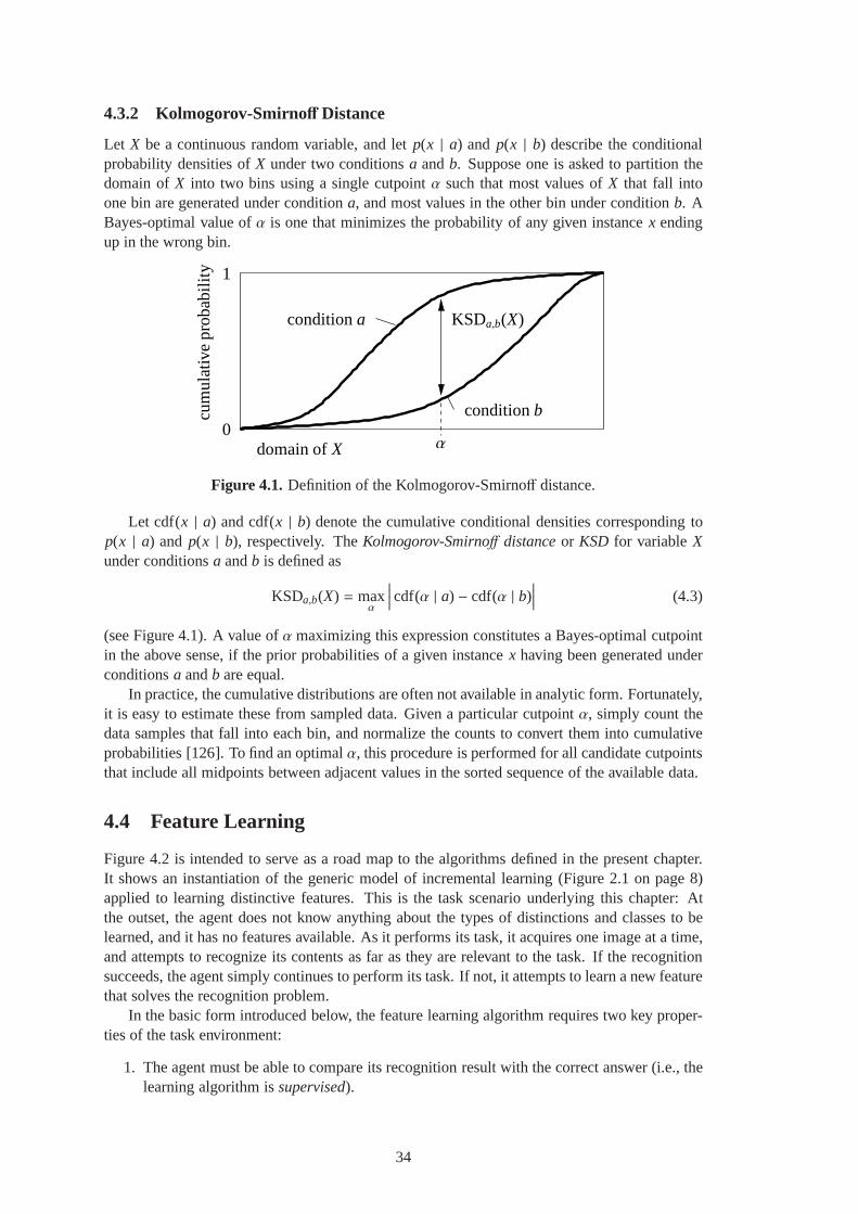
4.3.2 Kolmogorov-Smirnoff Distance

Let X be a continuous random variable, and letp(x | a) and p(x | b) describe the conditionalprobability densities ofX under two conditionsa andb. Suppose one is asked to partition thedomain ofX into two bins using a single cutpointα such that most values ofX that fall intoone bin are generated under conditiona, and most values in the other bin under conditionb. ABayes-optimal value ofα is one that minimizes the probability of any given instancex endingup in the wrong bin.

conditionb

conditiona

0

KSDa,b(X)

cum

ula

tive

pro

bab

ility

1

domain ofX α

Figure 4.1. Definition of the Kolmogorov-Smirnoff distance.

Let cdf(x | a) and cdf(x | b) denote the cumulative conditional densities corresponding top(x | a) and p(x | b), respectively. TheKolmogorov-Smirnoff distanceor KSD for variableXunder conditionsa andb is defined as

KSDa,b(X) = maxα

∣

∣

∣

∣

cdf(α | a) − cdf(α | b)∣

∣

∣

∣

(4.3)

(see Figure 4.1). A value ofα maximizing this expression constitutes a Bayes-optimal cutpointin the above sense, if the prior probabilities of a given instancex having been generated underconditionsa andb are equal.

In practice, the cumulative distributions are often not available in analytic form. Fortunately,it is easy to estimate these from sampled data. Given a particular cutpointα, simply count thedata samples that fall into each bin, and normalize the counts to convert them into cumulativeprobabilities [126]. To find an optimalα, this procedure is performed for all candidate cutpointsthat include all midpoints between adjacent values in the sorted sequence of the available data.

4.4 Feature Learning

Figure 4.2 is intended to serve as a road map to the algorithmsdefined in the present chapter.It shows an instantiation of the generic model of incremental learning (Figure 2.1 on page 8)applied to learning distinctive features. This is the task scenario underlying this chapter: Atthe outset, the agent does not know anything about the types of distinctions and classes to belearned, and it has no features available. As it performs itstask, it acquires one image at a time,and attempts to recognize its contents as far as they are relevant to the task. If the recognitionsucceeds, the agent simply continues to perform its task. Ifnot, it attempts to learn a new featurethat solves the recognition problem.

In the basic form introduced below, the feature learning algorithm requires two key proper-ties of the task environment:

1. The agent must be able to compare its recognition result with the correct answer (i.e., thelearning algorithm issupervised).

34

recognize classesAlgorithm 4.4

empty

acquire image

correct?yes no

learn distinctive featureAlgorithm 4.8,

using Algorithm 4.10

Algorithm 4.7

Figure 4.2. A model of incremental discrimination learning (cf. Figure2.1, page 8).

2. The agent must be able to acquire randomexample imagesof scenes containing instancesof specific classes. This permits statistical evaluation ofcandidate features.

The second requirement is not a critical limitation in many realistic interactive scenarios. Forexample, an infant can pick up a known object and view it from various viewpoints; or a childreceives various examples of letters of the alphabet from a teacher. A robot may aim its cameraat known locations, or may pick up a known object from a known location.

The subsequent sections introduce the key components of thevisual learning algorithm inturn; namely, the classifier subsystem, the recognition algorithm, and the feature learning pro-cedure.

4.4.1 Classifier

Conventionally, a Bayesian network classifier models the classes using a single discrete randomvariable that has one state for each class. This representation assumes that there is exactly onecorrect class label associated with each instance. Also, each feature – if instantiated – alwayscontributes to the classification process, no matter what the current class is, because each featurenode contains a full conditional probability table thatfor each classrepresents the probability ofthis feature being observed. This is contrary to the conceptof distinctive features that specializein specific distinctions between a characteristic class anda small subset of the other classes. In anaive Bayesian classifier, the number of entries contained in the probability table at each featurenode is equal to the product of the number of classes times thenumber of states of the featurevariable. If there are many classes, these tables can becomequite large. All their conditionalprobability entries must be estimated. Even worse, all of them must be re-estimated whenever anew class is added to the system.

A natural way to avoid these problems is to represent each class by an individual Bayesiannetwork classifier. An example is shown in Figure 4.3. The class node of each network hastwo states, representing presence or absence of an instanceof this class. Here, each feature ischaracteristic (in the sense of Definition 4.1, page 31) of the class represented by its Bayesiannetwork, and is discriminative with respect to one or more specific other classes. In Figure 4.3,all features are characteristic of classC, and the discriminated classes are shown inside thefeature nodes.

35

Class C

Feature 1−Class A

Feature 2

Feature 3Feature 5

Feature 4−Classes AB −Class E

−Class A

−Class B

Figure 4.3. A hypothetical example Bayesian network.

This representation keeps the classes and their characteristic features separate. When a newclass is learned, a corresponding network is instantiated,but the existing networks and theirconditional probability tables remain unaffected. Moreover, this representation builds in the as-sumption that the probability of the presence of each class is independent from all other classes.Since each network separately decides whether an object of its class is present, multiple targetclasses within a scene are easily handled without interference. Each network effectively acts asan objectdetectionsystem. In contrast, most current recognition systems act as classificationsystems and assign exactly one class label to each image.

Together with the concept of distinctive features, an important implication of this represen-tation is that the absence of a feature in an image never increases the belief in the presence of aclass. Inference in favor of a class is only drawn as a result of detected features. This behavioris a design choice reflecting the openness of the uncommittedlearning system. It is noteworthythat this design is in contrast to conventional recognitionsystems that always assign exactly oneof a given set of class labels to an image. Under this paradigm, calledforced-choicerecognitionby psychologists, not detecting a characteristic feature will inevitably increase the belief in thepresence of other classes. This effect may be desirable in aclosed world, but can be detrimentalin realistic open scenarios. Many conventional recognition systems adopt confidence thresholdsthat avoid the assignment of a class label in the absence of sufficient evidence for any class,which reduces but does not eliminate this problem.

Like class nodes, feature nodes also have two states, corresponding to presence or absenceof the feature. As in a typical naive Bayesian network classifier, arcs are directed from the classnode to the feature nodes. To model known dependencies between features, additional arcsconnect features where appropriate. Such dependencies arise by the construction of compoundfeatures. Specifically, if a geometric compound feature (say, Feature 3 in Figure 4.3) has a com-ponent feature that is also present in the network (e.g., Feature 2 in Figure 4.3), then it is clearthat the presence of Feature 3 implies a high probability of finding Feature 2 in the scene also.Feature 2 does not necessarily have to be present because thethresholds that define “presence”are determined independently for each feature node (see Definition 4.2 below). An analogousargument holds for the components of a conjunctive feature.In the case of a disjunctive feature,the direction of the argument – and that of the arcs – is reversed. Say, Feature 4 is a disjunctivefeature, and Feature 5 is one of its components. Then, findingFeature 5 in a scene implies thelikely presence of the disjunctive Feature 4 in the same scene. The reverse is not necessarilytrue because Feature 4 may be present by virtue of its other subfeature, with Feature 5 beingcompletely absent. Therefore, the causal influence is modeled by an arc from the componentfeature to the compound.

Note that the same feature (defined by its structure and its response vector) may occur inmore than one Bayesian network classifier. Feature values are measured using Equation 3.14

36

(page 25). Since these feature values are real numbers, theymust be discretized by applying athreshold marking the minimum value required of a feature inorder to be considered present.This threshold is determined individually for each featurenode so as to maximize its distinctivepower:

Definition 4.2 (Distinctive Power of a Feature) Thediscriminative powerof a featuref is theKolmogorov-Smirnoff distance (KSD) between the conditional distributions of feature valuesobserved under (a) the discriminated classes versus (b) the characterized class (cf. Equation 4.3and Figure 4.1). Thedistinctive powerof a feature is identical to its discriminative power, ifcdf(αf | a) > cdf(αf | b) for the cutpointαf associated with the KSD, i.e., the feature is in factcharacteristic of its class. Otherwise, the distinctive power is defined to be zero.

As was noted in Section 4.3.2, this definition yields an optimal cutpoint in the Bayesian sensethat if the presence of a class is to be inferred on the basis ofthis feature alone, the probabilityof error is minimized, given that the prior probability of the presence of this class equals 0.5.In general, however, the prior probability of a class will not be equal to 0.5. In this case, thischoice of a cutpoint is not optimal in any known sense. Nevertheless, Utgoff and Clouse [126]make a strong argument in favor of using the KSDwithout paying attention to the prior classprobabilitiesas a test selection metric for decision trees. It is based on the observation that evenin cases where the Bayesian choice is always the same regardless of the test, the cutpoint givenby the KSD separates two very different regions of certainty regarding the presence of the class.

Example 4.3 (KSD and Disparate Priors) Consider the class-conditional distributions shownin Figure 4.4. There are many more samples from the discriminated classes than from the

discriminated classes

characterized class

Distributions of feature values observed under the

freq

uenc

y co

unt

0 1feature values

Figure 4.4. Highly uneven and overlapping feature value distributions.

characterized class. In other words, given an unclassified sample, the prior probability that itbelongs to the discriminated classes is much higher than that it belongs to the characterized class.Where should the Bayes-optimal cutpoint be placed that allows one to guess what conditionaldistribution generated a given sample? The two distributions fully overlap! Because of this andthe disparate priors, it is clear from Figure 4.4 that no matter where a cutpoint is placed, theexpected error rate is minimized by always guessing that a sample came from the discriminatedclasses, irrespective of the sample’s feature value. However, it is also obvious that a cutpointcan be found that is meaningful in the sense that almost all samples of the characterized classfall above it, and almost none below it. While a decision rulebased on such a cutpoint is notBayes-optimal, this cutpoint would tell us something aboutthe posterior probability of a samplebelonging to each of the two conditional distributions. Utgoff and Clause simply suggest thatthe simple definition of the KSD given in Equation 4.3 be applied, which – being based oncumulative distributions – ignores the prior probabilities.

The computation of a KSD requires a description of the two conditional probability distri-butions. Here, these distributions are approximated by thecumulative experience of the agent:

37

The agent maintains aninstance listof experiences. Each image encountered adds to the in-stance list a newinstance vectorcontaining the feature values measured and the true class labelof this training image. All probability estimates relatingto the Bayesian network classifiers areestimated by counting entries in the instance list. This includes the cumulative distributionsfor estimating the KSDs to discretize feature variables, the conditional probability tables at thefeature nodes, and the prior class probabilities at the class nodes.

4.4.2 Recognition

Recognition of a scene can be performed in the conventional way by first measuring the strengthof each feature in the image, setting the feature nodes of theBayesian networks to the corre-sponding values, and computing the posterior probability of the presence of each class. In thiscase, the absence of a feature is meaningful to the system. Alternatively, robustness to occlu-sion can be built into the system by setting only feature nodes corresponding to found features,and leaving the others unspecified. In this case, the posterior probability of these features be-ing present (but occluded) can easily be computed. Incorporating positive evidence into thenet will monotonically increase the posterior probabilityof a class. In particular, the posteriorprobability is always greater than or equal to the prior. Without effective countermeasures how-ever, in practice this monotonic increase will often resultin very high posterior probabilities formany classes. Since the posterior class probabilities are computed independently by separatenetworks for each class, evidence found for one class does not reduce the posterior belief inany other class. To avoid these problems, in this work both positive and negative evidence isincorporated into the network by setting the applicable feature nodes to the corresponding state,presence or absence.

Computing a feature value in an image is expensive (cf. Equation 3.14) in comparison topropagating evidence in a Bayesian network of moderate size. Moreover, the contribution ofindividual features to the classification decision is unclear if all of them are computed at once.Therefore, features are computed sequentially, and the classification decisions are made incre-mentally within each Bayesian network, according to the following algorithm.

Algorithm 4.4 (Sequential Computation of Class Beliefs)

1. Bring the Bayesian network to equilibrium by propagatingevidence.

2. Find the maximally informative feature among all features of all classes. LetC and Ff

denote two-state random variables representing the presence or absence of a class andof a featuref , respectively. Then, the maximally informative featurefmax is the one thatmaximizes

Imax = maxf

maxC

I (C, Ff )

whereI (C, Ff ) is the mutual information defined in Equation 4.2 on page 33.

3. If Imax = 0, then stop.

4. Measure the value of this featurefmax, ffmax, in the current image using Equation 3.14.

5. Instantiate all nodes corresponding tofmax in all networks to the appropriate values bycomparingffmax against the respective thresholdsαf (cf. Definition 4.2).

6. To keep track of the usage of each feature, labelfmax with the running number of thecurrent training image. Then, continue with Step 1.

Note that at each iteration of this algorithm, one feature isinstantiated. For an instantiatedfeaturef , the uncertainty in its characterized classC is H(C) = H(C | Ff ), and thusI (C, Ff ) = 0(Equation 4.1). Therefore, the algorithm stops at Step 3 after all features have been instantiated.

38

In practice, it often stops sooner because among the uninstantiated features there are none withnonzero mutual information. This results if the entropies in all of the class nodes have beenreduced to zero, or if none of the remaining features are informative with respect to any classvariable with nonzero entropy. The labeling in Step 6 allowsthe algorithm to detect obsoletefeatures. If a feature ceases to be used, it can be discarded.This will further be discussed inSection 4.5.

There are various ways to add sophistication to this basic algorithm. Instead of consult-ing features exhaustively, a stopping criterion can be introduced that terminates Algorithm 4.4once I (C, Ff ) drops below a threshold at Step 2. By definition, features with low mutual in-formation have little potential to affect the posterior class distributions. The tradeoff betweencomputational expense and confidence in the recognition result can be adjusted in terms of thisthreshold. Another computational tradeoff concerns the relative cost of measuring feature val-ues. Large compound features consisting of many subfeatures are more costly to evaluate thansmaller features, as are Boolean compounds relative to geometric compounds (see Section 3.5.1on page 26, and Section 3.5.2). This cost can be considered atStep 2 of Algorithm 4.4, forexample using the framework of decision theory [102, 98]. Such thresholds and costs dependon specific applications. For simplicity, these issues are avoided here.

Since each class is represented by its own Bayesian network,the possibility of multipleclasses present in a scene is built into the system. The presence of each class is determinedindependently of all others. The possibility of arbitrary numbers of target classes within a scenemakes the evaluation of recognition results somewhat more complicated than the conventionalcorrect/wrong dichotomy. A recognition result is derived from the posterior class probabilitiesaccording to the following definition:

Definition 4.5 (Evaluation of Recognition Results) Those classes with a posterior probabil-ity greater than 0.5 are said to berecognized. A class is calledtrue if it is present in the scene,andfalseotherwise. Each recognition falls into exactly one of the following categories:

correct: Exactly the true classes are recognized.

wrong: The correct number of classes are recognized, but these include at least one falseclass. At least one true class was missed.

ambiguous:All of the true classes are recognized, plus one or more falseclasses.

confused: None or some (but not all) of the true classes, and some false classes are recog-nized. The number of recognized classes is different from the number of targetclasses present in the scene. (Otherwise, it is considered awrongrecognition.)

ignorant: None or some (but not all) of the true classes, and none of the false classes arerecognized.

The category ofwrongrecognitions constitutes a special case of misrecognitions that are other-wise in theconfusedcategory. Wrong recognitions are important in that they contain pairwiseerrors where one class is mistaken for one other class. In a classical forced-choice scenario, thisis the only type of incorrect recognitions.

In conventional forced-choice classification, there are only correct and wrong categories.Since this system has the additional freedom to assign multiple class labels or no label at all,the number of correct recognitions may be lower than in a forced-choice situation. To facilitatecomparison with forced-choice scenarios, at least the number of ambiguous recognitions shouldsomehow be taken into account. These contain the right answer, which is valuable especially ifthe number of false positive labels in an ambiguous recognition is low. Similarly, an ignorantrecognition should contribute to the same extent as a randomresult. This idea is formalized inthe following definition.

39

Definition 4.6 (Accuracy) A recognition resultis a set of classes recognized in an imageI byAlgorithm 4.4. This set includesnt true positives andnf false positives, wherent + nf ≤ nc, thetotal number of classes known to the system. LetnT denote the actual number of target objectsdepicted in the scene. Then,

acc(I ) =

nT

ncif nt + nf = 0

nt

nT + nfotherwise

is theaccuracyof this recognition result. The accuracy achieved on a setI of images is givenby

acc(I) =1|I|

∑

I∈Iacc(I ).

This definition is a generalization of the notion of correct recognition that values ambiguousrecognitions according to the number of false positives involved. An ignorant recognition isregarded as equivalent to a fully ambiguous recognition, i.e., a result that lists allnc class la-bels. The accuracy is a value between zero and one, where the maximum corresponds to 100%correct recognition. If all recognitions are ignorant or fully ambiguous, then the accuracy is theinverse of the number of classes known to the system. IfnT = 1 everywhere, this is identical tothe chance-level proportion of correct recognitions attained by uniformly random forced-choiceclassifiers. Thus, the accuracy can be directly compared to the percentage-correct result deliv-ered by a conventional forced-choice classifier.

4.4.3 Feature Learning Algorithm

In the incremental learning scenario (Figure 4.2 on page 35), the agent receives training imagesone by one. Initially, the agent does not know about any classes or features. When it is presentedwith the first image, it simply remembers the correct answer.When it is shown the secondimage, it will guess the same answer. This will continue, andno features will be learned, untilthis answer turns out to be incorrect.

Algorithm 4.7 (Operation of the Learning System) This algorithm provides details of thebasic model of incremental discrimination learning shown in Figure 4.2, page 35.

1. A new training image is acquired, denotedI .

2. ImageI is run through the recognition algorithm 4.4 as described inSection 4.4.2. Ifrecognition is correct according to Definition 4.5, then continue at Step 1.

3. Assume recognition failed because of inaccurate conditional probability estimates storedin the Bayesian networks. To remedy, all feature nodes are re-discretized to maximizetheir distinctive power (cf. Definition 4.2, page 37). Theirconditional probabilities areestimated by counting co-occurring feature values and class labels in the instance list (cf.Section 4.4.1, page 38). In the same way, the prior probabilities associated with the classnodes are re-estimated.

4. Re-run the recognition algorithm 4.4 on the imageI . If I is now recognized correctly, thencontinue at Step 1.

5. Conclude that at least one new feature must be added to at least one Bayesian network torecognizeI correctly. Attempt to do this by invoking Algorithm 4.8 (described below).Then, continue at Step 1.

40

This algorithm re-estimates the conditional probability tables of the Bayesian networks onlywhen an image is misrecognized (Step 3). Alternatively, after each recognition – successfulor otherwise – the conditional probability tables of all nodes related to queried features couldbe updated, maintaining a best estimate of the actual probabilities at all times. A drawbackof this approach is that the behavior of the system would fluctuate even in the absence of anymistakes. For example, two consecutive presentations of the same image could result in twodifferent recognition results. Since it is easier to characterize the behavior of the system if itsbehavior does not depend on a recent history of correct recognitions, it is designed to learn onlyfrom mistakes.

At Step 5 in this algorithm, the objective is to derive a new feature to discriminate one ormore true classes from one or moremistakenclasses, i.e., those false classes that were erro-neously recognized. Two cases must be distinguished. In thefirst case, a true class is not amongthe recognized classes (wrong, confused, or ignorant recognition). The agent needs to find anew feature of this true class in the current image – thesample image– that, if detected, willcause this class to be recognized. In the second case, some false classes were recognized inaddition to the true classes (ambiguous recognition). Here, the agent needs to find a feature inan image of a false class that is not present in the currently misrecognized image, and that, ifnot detected, will prevent this false class from being recognized. Again, this image is called thesample image.

Algorithm 4.8 (Feature Learning)

1. For the purpose of learning this feature, the true and mistaken classes are (re)defined sothat there is generally exactly one true and one mistaken class. The classes selected arethe true class with minimum belief and the false class with maximum belief, respectively,representing the most drastic case. In either case, if thereis no such unique class, beliefvalues from earlier (non-final) recognition stages (Algorithm 4.4) are consulted. In partic-ular, this covers the case of ignorant recognition. See below for further discussion and anexample.

2. A set ofexample imagesis retrieved from the environment. This set containsnex ran-dom views of each of the true class and the mistaken class. Theprecise value ofnex isunimportant, but involves a tradeoff that will be discussed below.

3. A new feature is generated, generally by random sampling from the sample image, usingAlgorithm 4.10. Algorithm 4.10 may be called only a limited number of times withina single execution of Algorithm 4.8. If this limit is exceeded, Algorithm 4.8 terminatesunsuccessfully. The details will be discussed below in the context of Algorithm 4.10.

4. A new node representing this new feature is added to the Bayesian network that models theclass of the sample image, along with an arc from the class node and any arcs required toor from any other feature nodes, to model any known interdependencies with pre-existingfeatures (cf. Section 4.4.1).

5. The values of this feature, as well as any existing features represented by nodes linked toor from the new feature node in the Bayes network, are measured within each exampleimage. The resulting instance vectors are added to the instance list.

6. The new feature node is discretized such that the cutpointmaximizes the distinctive powerbetween the true and mistaken classes (see Definition 4.2 on page 37), as estimated bycounting entries in the instance list. If the distinctive power is zero, the algorithm continuesat Step 3.

7. The conditional probability tables of the affected nodes are (re)estimated by counting en-tries in the instance list.

8. The recognition procedure (Algorithm 4.4) is run on the sample image, using the addedfeature.

41

(a) If the sample image is of a true class that is erroneously not recognized, or if the sam-ple image is of a false class that is erroneously recognized,then the new feature nodeis removed from the Bayes net. However, the definition of the new feature (consist-ing of its structural description and response vector) is retained until this algorithmterminates. Now, it proceeds with Step 3.

(b) If the image is of a true class and is now recognized successfully, or if it is of a falseclass and is successfully not recognized, then this algorithm terminates successfully.

Note that this feature search procedure requires that each new feature individually solves anexisting recognition problem. This results in a strong tendency to learn few but informativefeatures. Each feature is learned specifically to distinguish one class from one other class (seeStep 1). Instead of using just one true and one mistaken class, one could use all misrecognizedclasses, or even all true and false classes. However, in general it will be much easier to findfeatures that discriminate well between pairs of classes, than features that discriminate betweentwo groups of several classes. In practice, this may in fact be all that is required to solve agiven visual task. Moreover, using only a pair of classes ensures that the execution time of thisalgorithm is independent of the total number of classes.

Example 4.9 (Selecting True and Mistaken Classes)Table 4.1 shows some examples of howthe characterized and discriminated classes are chosen in Step 1 of Algorithm 4.8. The first caseshows a wrong recognition result. Since all classes with posterior beliefs greater than 0.5 aresaid to be recognized, the system erred on classes B and C. Here, it is clear that a new featureneeds to be learned for class B that will cause class B to be recognized in the current image.This new feature should be discriminative with respect to class C, because the system mistookclass B for class C. Note that the new feature will not affect the recognition result for class C(nor for any other class but the characterized class B). Likely, it will cause an ambiguous resultlike that shown in the second row. Now, a feature must be learned that is characteristic of classC, and that, if not found in an image, will prevent it from being recognized as class C. ClassA is chosen as the discriminated class because it has the lowest posterior belief among all trueclasses, and is therefore presumably most likely confused with class C.

Table 4.1. Selecting true and mistaken classes using posterior class probabilities. Bold typeindicates the characterized class of the new feature to be learned. The discriminated classes areshown in italics.

True Classes False ClassesA B C D E

wrong 0.7 0.4 0.8 0.3 0.2ambiguous 0.7 0.9 0.8 0.3 0.2ignorant 0.3 0.4 0.4 0.3 0.2

0.4 0.4 0.3 0.3 0.2ignorant 0.0 0.0 0.0 0.0 0.0

The first (wrong) example would constitute a confused recognition if, for example, class D hadreceived a posterior belief of greater than 0.5. The third example is an ignorant recognition.Like in wrong and confused cases, the characteristic class is the true class with lowest posteriorbelief, and the discriminated class is the false class with highest posterior belief. In the finalexample, Algorithm 4.4 resulted in zero belief for all classes. In such a case where true andcharacteristic classes cannot be determined from the final recognition result, the system consultsthe intermediate recognition result generated by the penultimate iteration of Algorithm 4.4. Thisresult is guaranteed to contain beliefs with nonzero entropy. In this example, there are two

42

potential characteristic classes because both true classes have identical belief. In this case, oneof them is chosen at random because Algorithm 4.4 requires a single sample image. Thereare also two potential discriminated classes, both of whichare simply used. In practice, suchambiguous cases occur very rarely.

The number of example images per class,nex (Algorithm 4.8, Step 2), determines how ac-curately the conditional probabilities associated with the new feature are estimated at Step 7. Alarge value yields accurate estimates, but these are expensive to evaluate. The danger of usingtoo small a value ofnex is that many good features are discarded because of overly pessimisticprobability estimates. Optimistic estimates result in theaddition of features that later turn outto be of little value. Consequently, these will cease to be used as they are superseded by morediscriminative features. Thus, using a smallnex will result in more feature searches, each ofwhich will take less time than when using a largenex. In a practical interactive application, thechoice of this parameter should depend on the relative cost of acquiring images vs. generatingexperience in the real world. If experience is costly to obtain (e.g. because it involves sophisti-cated maneuvers with physical manipulators), but a varietyof representative images are cheaplyobtained at Step 2 of Algorithm 4.8, thennex should be chosen large. On the other hand, if eachreal-world experience is generated cheaply but example images are expensive to obtain, then asmall value ofnex should be used. The value does not need to be fixed, nor does it need to be thesame for the true and the mistaken class. All experiments reported here usenex = 5. This valuewas chosen relatively small because it emphasizes the incremental nature of learning even if asmall, fixed training set is used. At the other extreme,nex could be chosen so large that the ex-ample images always include the entire training set (so it exists), yielding immediately accurateestimates of the distinctive power of features without the need for incremental updating.

It remains to be explained how a feature is generated at Step 3of Algorithm 4.8. Thereare five ways to generate a new feature that differ in the structural complexity of the resultingfeature. In accord withOccam’s razor, simple features are preferred over complex features.Also, they are more likely to be reusable and are computed more rapidly than complex features.The following algorithm implements a bias toward structurally simple features by consideringfeatures in increasing order of structural complexity.

Algorithm 4.10 (Feature Generation) These methods are applied in turn at Step 3 of Algo-rithm 4.8:

1. (Reuse)From a Bayesian network representing an unrelated class (other than the true ormistaken classes), select a random feature that is not in usefor the true or mistaken classes,to see if it can be reused for the current recognition problem. This promotes the emergenceof general features that are characteristic of more than oneclass.

2. (New Primitive) Sample a new feature directly from the sample image by eitherpickingtwo points and turning them into a geometric compound of two edgels, or by picking onepoint and measuring a texel feature response vector. (Recall that features are measuredunder rotational invariance. Therefore, individual edgels do not carry any information.)This is the only step where new features are generated from scratch.

3. (Geometric Expansion)From among the features currently in use, or from among thefailed candidate features tried earlier during this execution of Algorithm 4.8 (see Algo-rithm 4.8, Step 8a), choose a feature at random. Find a location in the sample image wherethis feature occurs most strongly (Equation 3.14), and expand it geometrically by addinga randomly chosen salient edgel or texel nearby. This expansion yields a new feature thatis more specific than the original feature.

4. (Conjunction) Pick two random existing features and combine them into a conjunctivefeature. Again, the result is a new feature that is more specific than either of the constituentfeatures individually.

43

5. (Disjunction) Pick two random existing features and combine them into a disjunctivefeature. Here, the result is a new feature that is less specific than the constituent features.

For a given run of Algorithm 4.8 (Feature Learning, page 41),each time Algorithm 4.8reaches its Step 3, one method of Algorithm 4.10 is applied. The firstnfgen times Algorithm 4.8reaches Step 3, Method 1 of Algorithm 4.10 is performed; the next nfgen times, Method 2, andso on. This continues until either a suitable feature is found, or until the last method has beenappliednfgen times, at which point the feature search (Algorithm 4.8) terminates unsuccessfully.The parameternfgen in effect controls the bias toward simple features. A large value will expendmore effort using each method, while a small value will give up soonerand move on to the nextmethod. The current implementation usesnfgen = 10, which is considered to be a relativelysmall value in relation to the roughly 100–1000 salient points present in typical images usedhere (cf. Chapter 3).

The specific sequence of methods defined in Algorithm 4.10 waschosen because it imple-ments a bias toward few and structurally simple features. A new feature is only generated ifthe system fails to find a reusable feature. Before existing features are expanded, new primitivefeatures are generated. Geometric expansions are preferred over conjunctive features becausethe former are local and rigid, while the latter can encompass any variety of individual features.Local features are more robust to partial occlusions and minor object distortions than are non-local features. Nevertheless, conjunctive features may beimportant because they encode thepresence of several subfeatures without asserting a geometric relationship between them. Thismakes them more robust to object distortions than geometricfeatures.

The last step involves the generation of disjunctive features. These are susceptible to overfit-ting because a single disjunctive feature can in principle encode an entire class as a disjunctionof highly specific features, each characterizing an individual training image. Thus, they can helplearn a training set without generalization. On the other hand, disjunctive features are necessaryin general because objects within a class may differ strongly in their appearance. For example, adisjunctive feature can encode a statement such as “If I see adial or a number pad, I am probablylooking at a telephone.”

4.4.4 Impact of a New Feature

In Algorithm 4.8 (Feature Learning), Step 3, a new feature isgenerated in the hope that it will fixthe recognition problem that triggered the execution of Algorithm 4.8. Clearly, a necessary con-dition for success is that the new feature is actually consulted by the recognition algorithm 4.4,when called at Step 8 of Algorithm 4.8. Algorithm 4.4 continues to consult features as long asthere are features that can potentially reduce the uncertainty in any class nodes. Therefore, thenew feature will be queried if the entropy in its own class node does not vanish as a result ofquerying other features of this Bayesian network. The only way Algorithm 4.4 can terminatewithout querying the new feature is if there is a featuref in this Bayesian network that drivesthe entropy in its class node to zero, and that has a greater mutual information with respect tothe class node than the new feature, causing it to be queried before the new feature. Note thatthis recognition is incorrect, as it triggered the present execution of the feature learning algo-rithm 4.8 at Step 5 of Algorithm 4.7 (Operation of the Learning System). The newly generatedfeature is not going to be used on this image, irrespective ofany discriminative power it mayhave.

How likely is this worst-case situation to occur? Consider acase where the system failed torecognize a true class. Figure 4.5 illustrates the class-conditional cumulative probabilities of afeaturef that can drive the entropy in the class node to zero, concluding that its class is absent.The critical property of the graph is that if the class is present, the featuref is always present withff > α, allowing one to infer the absence of the class ifff ≤ α. (The figure also illustrates that

44

cum

ula

tive

pro

bab

ility

1

αf0 1

class absent

class present

ff

Figure 4.5. KSD of a featuref that, if not found in an image, causes its Bayesian network toinfer that its class is absent with absolute certainty.

the KSD of such a feature can be quite low – roughly 0.5 in this case.) Can this feature preventthe successful generation of new features by keeping them from getting queried? The answeris no because it will quickly lose its power to reduce the entropy to zero. To see this, observethat each processed image generates an instance that is added to the instance list, recordingthe measured feature values together with the true class labels. In the situation described here,ff ≤ αf , but the class was present. This situation is incompatible with the critical propertyof Figure 4.5. Consequently, the next time the conditional probabilities off are re-estimatedbased on the instance list, at least one of two changes must occur: The probability offf ≤ αf

given the presence of the class becomes greater than zero, orthe thresholdαf is reduced. Inthe first case, the feature immediately loses its power to determine the absence of the class withabsolute certainty. The second case clearly cannot reoccurindefinitely becauseαf is chosen tomaximize the KSD, ensuring thatff < αf for the bulk of those cases where the class is absent.As specified in Algorithm 4.7 (Operation of the Learning System) on page 40, the cutpointsαand the conditional probability tables of all feature nodesare re-estimated after every incorrectrecognition.

In summary, a newly sampled feature is not guaranteed to be used immediately. However,those cases where it is not used can be expected to be rare, since they require the presence of afeaturef with the specific properties described above. Importantly,any such degenerate situationis guaranteed to resolve itself soon because the feature node parameters are re-estimated afterevery incorrect recognition. This self-repairing property is a key aspect of the design of thelearning algorithm, and is critical to its successful operation.

4.5 Experiments

The algorithms developed in the preceding sections were developed for open task scenarios inwhich images are encountered while the agent performs a task. In effect, each newly acquiredvisual scene first serves as a test image that the agent attempts to recognize. If it succeeds, theagent moves on. If the result of recognition is incorrect, this scene becomes a training image.Additional example images are then acquired to enable the agent to generate an initial estimateof the distinctive power of newly generated features.

Testing this algorithm on such an interactive task is a nontrivial endeavor. Implementinga robot that can interact in meaningful ways with many objects is challenging in its own rightand beyond the scope of this dissertation. The results citedin this section were generated onsimulated tasks.

A second simplification concerns the number of objects shownin an image. The algorithmsdescribed above make no assumptions regarding the number oftarget or distractor objects shownpresent in any given image. For simplicity and to facilitatecomparison of the results with

45

conventional methods, all experiments were performed in the conventional way, with each imagecontaining exactly one object. It is important to note however that the learning system didnot take advantage of this in any way. The algorithms were applied in their full generality asintroduced above.

A simulated task consists of a closed set of images. This set of images was divided intoequally sized training and test sets, such that the number ofimages per class was identical tothe extent possible. Each experiment was run a second time with the roles of training and testsets reversed. In the machine learning terminology, this procedure is called two-fold stratifiedcross validation. Training took place as shown in the overview given in Figure 4.2 on page 35,and as described in detail in Section 4.4.3. Images from the training set were presented to thesystem one by one, cycling through the training set in randomorder. A new permutation wasused for each cycle. On receipt of an image, the system analyzed it using Algorithm 4.4. If therecognition result was not correct (in the sense of Definition 4.5 on page 39), then a new featurewas sought according to Algorithm 4.8. At Step 2 of this algorithm, the example images werechosen at random from the training set (not from the cycling order). The system cycled throughthe entire training set until all recognition results were correct.

The empirical performance of the learning system are discussed in terms of the evaluationcategories given in Definition 4.5, which apply to the general case of an arbitrary number oftarget classes. Since all experiments were performed usingonly a single target class, thesecategories are restated here for this special case, to simplify their interpretation.

correct: Exactly the true class is recognized.

wrong: Exactly one false class is recognized.

ambiguous:The true class is recognized, plus one or more false classes.

confused: More than one false classes are recognized, but not the true class.

ignorant: No class is recognized.

Experiments were conducted using three data sets with very different characteristics. These willbe discussed in the following sections. The next chapter will introduce a simple extension to thebasic learning algorithm that results in pronounced performance improvements.

4.5.1 The COIL Task

The COIL task consisted of 20 images of each of the first six objects of the 20-object ColumbiaObject Image Library [79]. One sample image of each class, representing the middle view,is shown in Figure 4.6. Neighboring views are spaced 5 degrees apart, at constant elevation.Neighboring images were assigned alternately to training and test sets. All images are of size128× 128 pixels.

obj1 obj2 obj3 obj4 obj5 obj6

Figure 4.6. Objects used in the COIL task. Shown are middle views from thesorted sequenceof viewpoints.

46

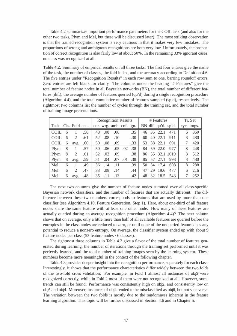
Table 4.2 summarizes important performance parameters forthe COIL task (and also for theother two tasks, Plym and Mel, but these will be discussed later). The most striking observationis that the trained recognition system is very cautious in that it makes very few mistakes. Theproportions of wrong and ambiguous recognitions are both very low. Unfortunately, the propor-tion of correct recognition is also fairly low at about 50%. In the remaining 33% ignorant cases,no class was recognized at all.

Table 4.2.Summary of empirical results on all three tasks. The first four entries give the nameof the task, the number of classes, the fold index, and the accuracy according to Definition 4.6.The five entries under “Recognition Results” in each row sum to one, barring roundoff errors.Zero entries are left blank for clarity. The columns under the heading “# Features” give thetotal number of feature nodes in all Bayesian networks (BN),the total number of different fea-tures (dif.), the average number of features queried (qu’d)during a single recognition procedure(Algorithm 4.4), and the total cumulative number of features sampled (sp’d), respectively. Therightmost two columns list the number of cycles through the training set, and the total numberof training image presentations.

Recognition Results # Features Tr. SetTask Cls. Fold acc. cor. wrg. amb. cnf. ign. BN dif. qu’d. sp’d. cyc. imgs.

COIL 6 1 .58 .48 .08 .08 .35 46 35 22.1 471 6 360COIL 6 2 .61 .52 .08 .10 .30 60 40 22.1 911 8 480COIL 6 avg. .60 .50 .08 .09 .33 53 38 22.1 691 7 420Plym 8 1 .57 .50 .06 .05 .02 .38 84 59 22.0 977 8 448Plym 8 2 .61 .52 .02 .09 .38 86 55 32.1 1019 8 512Plym 8 avg. .59 .51 .04 .07 .01 .38 85 57 27.1 998 8 480Mel 6 1 .49 .36 .14 .11 .39 50 34 17.4 608 8 288Mel 6 2 .47 .33 .08 .14 .44 47 29 19.6 477 6 216Mel 6 avg. .48 .35 .11 .13 .42 48 32 18.5 543 7 252

The next two columns give the number of feature nodes summed over all class-specificBayesian network classifiers, and the number of features that are actually different. The dif-ference between these two numbers corresponds to features that are used by more than oneclassifier (see Algorithm 4.10, Feature Generation, Step 1). Here, about one-third of all featurenodes share the same feature with at least one other node. Howmany of these features areactually queried during an average recognition procedure (Algorithm 4.4)? The next columnshows that on average, only a little more than half of all available features are queried before theentropies in the class nodes are reduced to zero, or until none of the unqueried features has anypotential to reduce a nonzero entropy. On average, the classifier system ended up with about 9feature nodes per class (53 feature nodes/ 6 classes).

The rightmost three columns in Table 4.2 give a flavor of the total number of features gen-erated during learning, the number of iterations through the training set performed until it wasperfectly learned, and the total number of training images seen by the learning system. Thesenumbers become more meaningful in the context of the following chapter.

Table 4.3 provides deeper insight into the recognition performance, separately for each class.Interestingly, it shows that the performance characteristics differ widely between the two foldsof the two-fold cross validation. For example, in Fold 1 almost all instances ofobj3 wererecognized correctly, while in Fold 2 most of them were not recognized at all. However, sometrends can still be found: Performance was consistently high on obj2, and consistently low onobj6 andobj4. Moreover, instances ofobj4 tended to be misclassified asobj6, but not vice versa.The variation between the two folds is mostly due to the randomness inherent in the featurelearning algorithm. This topic will be further discussed inSection 4.6 and in Chapter 5.

47

Table 4.3. Results on the COIL task. The table shows, for each class, howmany instanceswere recognized as which class for correct and wrong recognitions, and the number of ambigu-ous/confused/ignorant recognition outcomes. In each row, these entries sum to the number oftest images of each class (here, 10). The rightmost column shows the number of feature nodesthat are part of the Bayesian network representing each class. The bottom row of the bottompanel gives the average proportion of the test set that fallsinto each recognition category.

Confusion Matrix correct/wrong # Feats.Class obj1 obj2 obj3 obj4 obj5 obj6 amb. cnf. ign. BN

Fold 1:obj1 6 4 8obj2 8 1 1 4obj3 8 2 9obj4 1 2 1 2 2 2 11obj5 3 2 5 5obj6 1 2 7 9Sum 6 8 10 2 4 4 5 0 21 46

Fold 2:obj1 5 5 10obj2 10 7obj3 2 1 7 16obj4 4 2 2 2 9obj5 7 2 1 8obj6 2 3 2 3 10Sum 5 10 2 4 10 5 6 0 18 60

Average of both folds (proportions):obj1 .55 .45 9obj2 .90 .05 .05 6obj3 .50 .05 .45 13obj4 .05 .30 .05 .20 .20 .20 10obj5 .50 .20 .30 7obj6 .05 .10 .25 .10 .50 10Avg. .09 .15 .10 .05 .12 .08 .09 .00 .33 9

48

In the cases of ambiguous recognition, which classes were the false positives? The answeris given by Table 4.4. In both folds,obj4 andobj5 could often not be disambiguated from eachother. These wrong and ambiguous recognitions do not seem intuitive, given that they appearvery dissimilar to a casual observer (Figure 4.6). However,in Fold 1, obj4 shares one featurewith each ofobj5 andobj6. This is an indication that at some level, these classes do seem similarto the learning system. Even more strongly in Fold 2,obj4 shares one feature withobj5, twofeatures withobj6, and one more feature with bothobj5 and obj6. Examples of the featureslearned for each class are shown in Figure 4.7. Edgels and texels and their orientations andscales are represented as in Figure 3.9 on page 22. In addition, the subfeatures of a compoundfeature are linked with a line, that is solid for geometric and dotted for Boolean compounds.

Table 4.4.Results on the COIL task: Confusion matrices of ambiguous recognitions. The italicnumbers on the diagonal indicate how many times the class given on the left was recognizedambiguously (cf. Table 4.3), and the upright numbers in eachrow specify the false-positiveclasses.

Class obj1 obj2 obj3 obj4 obj5 obj6

Fold 1:obj1obj2 1 1obj3obj4 2 1 1obj5 1 1 2obj6

Fold 2:obj1obj2obj3obj4 2 2 1obj5 1 2 1obj6 1 1 2

To a casual human observer, the two cars (obj3 andobj6) look very similar. Why does thelearning system not seem to have any difficulty with these two objects? The answer is thatthe similarity occurs at a high level, concerning the overall shape of the body, the location ofthe wheels, etc. However, the learning system does not have direct access to these high-levelfeatures. It only looks at a small number of strongly localized features, and at combinations ofthese. At the level of local features, the two cars in fact look rather different even to humans.

What are the appearance characteristics captured by individual features? Figures 4.8 and4.9 give an intuition. Figure 4.8 shows all images of classobj1. Each image displays all featurescharacteristic of this class that is present in this image (i.e., ff > αf ; cf. Algorithm 4.4, Step 5,page 38). Each feature is annotated with a unique identifierk (featurek was thekth featurelearned by the system). The images show that some features are reliably located at correspond-ing parts of the duck (features 5, 8, 25). Other features change their location with the viewpoint(features 11, 13). Most features appear on most views, whilefeature 22 only occurs in a fewimages. Feature 9 is a disjunctive feature. In most views, its dominant subfeature is a large-scalegeometric compound of two edgels. Only the first image shows its other subfeature, a texel.

Figure 4.9 illustrates the specificity of a representative subset of the features characteristicof classobj1. The two center columns indicate how strongly a feature responded everywhere inthe image. For purposes of illustration, the feature response value was computed at all imagepoints (not just at salient points). At each point, all scales corresponding to scale-space maxima

49

Figure 4.7. Examples of features learned for the COIL task. For each class, all features char-acterizing this class in Fold 1 are shown that are consideredto be present in the image by theclassifier.

50

Figure 4.8. Features characteristic ofobj1 located in all images of this class where they arepresent. These features were learned in Fold 1, and are here identified by unique ID numbers.

51

were considered. The gray value at a pixel corresponds to themaximum feature valuefmax overthese scales. The location of a feature is identified with thelocation of its reference point (cf.Figure 3.12, page 26). To enhance detail, the gray value is proportional tof 4

max, as most featureresponses are quite close to unity. A pixel was left white if the scale function did not assumeany local maxima at this image location. The figure shows thatsome features are more specificthan others. Feature 13 is the least specific feature characteristic ofobj1. It responds strongly inmany areas both around the periphery and in the interior of the duck, and also the cat. Feature 5is the most specific feature ofobj1, and responds primarily to certain areas interior to the duck.This feature is very similar to feature 25. Not accidentally, feature 13 assumed its strongestresponse at various places in Figure 4.8, while features 5 and 25 are stable with respect to theirlocation. Feature 18 is an example of an edge feature. In fact, its response is much more stronglylocalized to edges than the texel features shown in Figure 4.9. Feature 9 responds only weaklyeverywhere, as its constituent features were sampled from other images. Its presence thresholdαf is correspondingly lower (not shown in the figure).

4.5.2 The Plym Task

The second task used eight artificially rendered, geometricobjects,2 that are shown in Figure4.10. There are 15 views per object, covering a range of±10 degrees about the vertical axis rel-ative to the middle position shown in Figure 4.10 in steps of two degrees, at constant elevation.Two views are rendered from elevations 10 degrees above and below the middle position, andtwo views at 10 degrees in-plane rotation. The object surfaces are free of texture. This makesthe Plym task difficult to learn using the feature space used here, as the only discriminant infor-mation available to the learning system is given by local contour shading and angles betweenedges – and both are adversely affected by perspective distortions. The rendering viewpoints arecloser together and cover a smaller section of the viewing sphere than the COIL task. Again,neighboring views were assigned alternately to training and test sets, yielding one training/testset with 8 and one with 7 images per class. The objects are rendered at similar size, and theimages were cropped to leave a 16-pixel boundary around the object, resulting in image sizes ofabout 100× 170 pixels.

Table 4.2 reveals that the performance of the learning system on the Plym task was verysimilar to the COIL task. There was about the same number of correct recognitions, but slightlyfewer wrong and ambiguous recognitions, which is reflected by a higher proportion of ignorantresults. One of the very fewconfusedrecognition results ever encountered occurred here: Acucon was recognized as acucy and acyl3. Incidentally, in this fold thecucon Bayesian networkshared one feature each with each of thecucy and cyl3 networks, which indicates that theseclasses were considered similar by the learning system. Allother numbers shown in Table 4.2are roughly in proportion to the COIL task.

The confusion matrices (Table 4.5) again reveal striking consistencies and differences be-tween the two folds. For example,cyl3 was perfectly recognized in Fold 1, but poorly in Fold 2.Objectcycu was almost perfectly recognized in both folds. This object is characterized by aunique rectangular protrusion attached to a smooth surface. This turned out to be a powerfulclue to the learning system: The compound feature (from Fold2) sitting precisely at the attach-ment location in Figure 4.11 has a KSD of 1.0 – it is a perfect predictor of this object. In Fold 1,a coarse-scale texel feature was learned that responds to the unique concavity created by theprotrusion. This feature (not shown) also has a KSD of 1.0.

The consistently most difficult objects to recognize werecyl6 andtub6. Most severely, noneof these was recognized correctly in Fold 1. It is no coincidence thatcyl6 is the most featurelessobject in the dataset, and it is identical to thetub6 except that the latter is hollow. This is a

2These objects were generated by Levente Toth at the Centre For Intelligent Systems, University of Plymouth,UK, and are available under the URL http://www.cis.plym.ac.uk/cis/levi/UoP CIS 3D Archive/8obj set.tar.

52

Figure 4.9. Spatial distribution of feature responses of selected features characteristic ofobj1(left columns), for comparison also shown forobj4 (right columns). In the center columns,the gray level encodes the response strength of the feature shown in the outer panels. Blackrepresents the maximal response off = 1.0; in white areas no response was computed. Featuresare labeled by their ID numbers.

53

con6 cube cucon cucy cycu cyl3 cyl6 tub6

Figure 4.10.Objects used in the Plym task. Shown are middle views from thesorted sequenceof viewpoints.

con6 cube cucon cucy

cycu cyl3 cyl6 tub6

Figure 4.11. Examples of features learned for the Plym task. For each class, all features char-acterizing this class in Fold 2 are shown that are consideredto be present in the image by theclassifier.

54

Table 4.5. Results on the Plym task. The table shows, for each class, howmany instanceswere recognized as which class for correct and wrong recognitions, and the number of ambigu-ous/confused/ignorant recognition outcomes. In each row, these entries sum to the number oftest images of each class (here, 8 in Fold 1 and 7 in Fold 2). Therightmost column shows thenumber of feature nodes that are part of the Bayesian networkrepresenting each class. Thebottom row of the bottom panel gives the average proportion of the test set that falls into eachrecognition category.

Confusion Matrix correct/wrong # Feats.Class con6 cube cucon cucy cycu cyl3 cyl6 tub6 amb. cnf. ign. BN

Fold 1:con6 6 2 13cube 3 5 16cucon 1 5 1 1 5cucy 3 3 2 10cycu 7 1 8cyl3 8 4cyl6 8 15tub6 2 1 5 13Sum 7 3 5 3 7 10 1 0 3 1 24 84

Fold 2:con6 4 3 6cube 5 2 12cucon 1 5 1 6cucy 3 4 7cycu 7 6cyl3 3 4 14cyl6 3 4 21tub6 1 3 3 14Sum 4 5 1 3 7 3 4 3 5 0 21 86

Average of both folds (proportions):con6 .67 .33 10cube .53 .47 14cucon .07 .40 .33 .07 .13 6cucy .40 .20 .40 9cycu .93 .07 7cyl3 .73 .27 9cyl6 .20 .80 18tub6 .13 .13 .20 .53 14Avg. .09 .07 .05 .05 .12 .11 .04 .03 .07 .01 .38 11

55

situation where the lack of a closed-world assumption (cf. Section 4.4.1) impairs recognitionperformance: The only way to decide that an object is acyl6 as opposed to atub6 is by assertingtheabsenceof features corresponding to the cavity. This type of inference is not performed bythe recognition system. Therefore, the learning system tries hard to identify features characteris-tic of cyl6, finding features that respond to the individual training images, but do not generalize.These features fail to respond to unseen test views, which results in ignorant recognitions. Thesimilarity between these two objects is further illustrated by the fact that in both folds, theirrespective Bayesian networks share three features.

No pattern is apparent in the few ambiguous recognitions (Table 4.6). In each fold, only oneclass experienced ambiguous recognitions. Neither of these ambiguities is reflected in sharedfeatures.

Table 4.6.Results on the Plym task: Confusion matrices of ambiguous recognitions. The italicnumbers on the diagonal indicate how many times the class given on the left was recognizedambiguously (cf. Table 4.5), and the upright numbers in eachrow specify the false-positiveclasses.

Class con6 cube cucon cucy cycu cyl3 cyl6 tub6

Fold 1:con6cubecuconcucy 3 2 1cycucyl3cyl6tub6

Fold 2:con6cubecucon 1 5 4cucycycucyl3cyl6tub6

4.5.3 The Mel Task

The Mel task used all 12 images of each of six non-rigid objects from the image database usedto train and test Mel’s SEEMORE system [71]. All images are shown in Figure 4.12. To speedup processing, the images were subsampled to 320× 240 from their original size of 640× 480pixels. The views represent random samples from the objects’ configuration space, taken at twodifferent scales that differed by a factor of two. Images were randomly assigned to training andtest sets, each containing six images. This data set was intended to test the limits of the learningsystem. As the feature space derives most of its expressive power from geometric compoundfeatures, it is best suited for rigid objects. The Mel task, however, consists of non-rigid objectsin widely varying configurations, limiting useful geometric compounds to very small scales.

Table 4.2 shows that the system did poorly on the Mel database, as reflected by all perfor-mance categories except for confused recognitions. Ignorant recognitions even exceeded correct

56

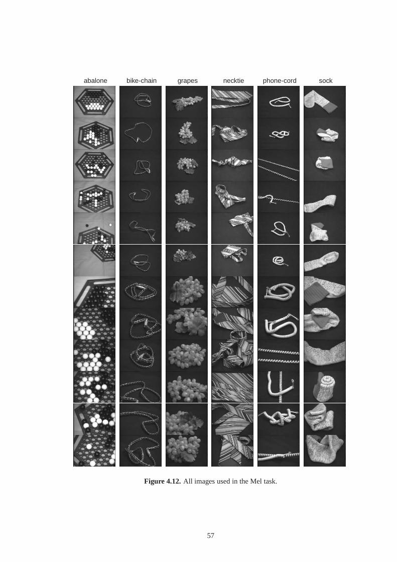
abalone bike-chain grapes necktie phone-cord sock

Figure 4.12.All images used in the Mel task.

57

recognitions. According to Table 4.7, the four weakest-performing classes werephone-cord,grapes, abalone, andsock. In particular, no phone cords were recognized correctly. One prob-lem was that for the smaller-scale views, much of the crucialdetail was represented at scales thatapproached the pixel size. Each of the other three classes reveals a limitation of the system aspresented here. Asock is primarily characterized by the gray-level statistics ofits structurelesssurface. However, the features described in Chapter 3 are designed to characterize gray-levelstructure, not statistics.

Table 4.7. Results on the Mel task. The table shows, for each class, how many instanceswere recognized as which class for correct and wrong recognitions, and the number of ambigu-ous/confused/ignorant recognition outcomes. In each row, these entries sum to the number oftest images of each class (here, 6). The rightmost column shows the number of feature nodesthat are part of the Bayesian network representing each class. The bottom row of the bottompanel gives the average proportion of the test set that fallsinto each recognition category.

Confusion Matrix correct/wrong # Feats.Class abalone chain grapes necktie cord sock amb.cnf. ign. BN

Fold 1:abalone 2 2 2 10bike-chain 4 2 8grapes 2 1 3 7necktie 1 3 2 7phone-cord 1 1 4 9sock 2 2 1 1 9Sum 3 5 2 5 1 2 4 0 14 50

Fold 2:abalone 2 1 3 6bike-chain 4 2 6grapes 1 1 1 3 7necktie 3 3 8phone-cord 1 5 12sock 2 1 3 8Sum 3 5 1 3 0 3 5 0 16 47

Average of both folds (proportions):abalone .33 .25 .42 8bike-chain .67 .33 7grapes .08 .25 .08 .08 .50 7necktie .08 .50 .25 .17 8phone-cord .08 .08 .08 .75 11sock .17 .33 .17 .33 9Avg. .08 .14 .04 .11 .01 .07 .13 .00 .42 8

Theabalone board contains strong gray-level structure, but this structure varies widely be-tween images (Figure 4.12). The most meaningful texel features occur about at the scale of theabalone balls. These do not have a meaningful orientation, as they will mostly be measuredat scales that are affected by changes in the board configuration. This prevents the construc-tion of powerful geometric compound features, as these relyon predictable relative orientationsbetween features.

For practical, reasons, the feature sampling procedure relies on salient points and their intrin-sic scales as extracted by scale-space methods. Thegrapes class exposes the critical impact of

58

this procedure on recognition performance. Due to the low contrast and the high degree of self-occlusion and clutter present in thegrapes images, the extracted texels and their scales rarelycorresponded to individual grapes. Moreover, similarly tothe abalone board, the orientationsof individual texels is rarely meaningful for larger-scaletexels in thegrape images.

Table 4.8 of ambiguous recognitions does not reveal any conclusive insights. Figure 4.13shows examples of features learned for the Mel task. Curiously, two background features werefound characteristic of theabalone class. From the viewpoint of task-driven learning, this is notconsidered bad. Any feature that is helpful on a task should be considered. If the background ispredictive of a target class, then background features may contribute to performance.

Table 4.8. Results on the Mel task: Confusion matrices of ambiguous recognitions. The italicnumbers on the diagonal indicate how many times the class given on the left was recognizedambiguously (cf. Table 4.7), and the upright numbers in eachrow specify the false-positiveclasses.

Class abalone chain grapes necktie cord sock

Fold 1:abalone 2 2 1bike-chaingrapesnecktiephone-cord 1 1sock 1 1

Fold 2:abalone 1 1bike-chaingrapesnecktie 1 1 3 1phone-cordsock 1 1 1

4.6 Discussion

This chapter presented an incremental and task-driven method for learning distinctive featuresfrom the feature space introduced in the previous chapter. Although the experiments describedabove used conventional data sets used in object recognition research, the method developedhere is far more general than most existing recognition systems. In contrast to most methodsbased on eigen-subspace decomposition, this approach doesnot rely on global appearance orbackground segmentation (but see Colin de Verdiere and Crowley [26] for an example of locallyapplied eigen-features, and Black and Jepson [14] and Leonardis and Bischof [61] for robustversions of global eigen-features). In contrast to most approaches based on local features, thissystem does not require a hand-built feature set, but learnsdistinctive features from a featurespace. No prior knowledge about the total number of target classes is used, and no assumptionsare made regarding the number of target classes present in any given image. The learner learnsdistinctions as required, adding classes as they arise.

The feature learning algorithm relies on two key concepts for incremental learning of condi-tional probabilities: the example images, and the instancelist. The concept of example imagesis analogous to the human capacity to keep a small number of example views in short-termmemory. A human acquires these views simply by looking at an object for an extended period

59

Figure 4.13. Examples of features learned for the Mel task. For each class, all features char-acterizing this class in Fold 1 are shown that are consideredto be present in the image by theclassifier.

60

of time while changing the viewpoint. Importantly, these acquired views are not distinct, butform a coherent motion sequence, which allows the observer to track features across viewpoints.This can greatly facilitate the discovery of stable and distinctive features [129]. In the systemdiscussed in the present chapter, no such assumptions are made about the example images. Fu-ture work should investigate how to take advantage of passively provided or actively acquiredmotion sequences.

Notably, example images can be avoided altogether. In this case, evaluation of newly sam-pled features is deferred until a sufficient number of training views of the object classes inquestion has been acquired over time. However, this deferred evaluation precludes the goal-directed, simple-to-complex feature search implemented by Algorithms 4.8 and 4.10. Instead, anumber of features must be generated and kept around until they can be evaluated. To illustratehow this can be implemented, the second application discussed in Chapter 6 operates withoutexample images.

The second key component, the instance list, is not easily dispensable because it is used toestimate class-conditional feature probabilities. The dynamic recomputation of the thresholdsαf (cf. Definition 4.2 (Distinctive Power of a Feature) on page 37, and Algorithm 4.8 (FeatureLearning), Step 7 on page 41) relies on the ability to count the individual instances. However,this dynamic recomputation is not an essential part of the overall algorithm. If one is willing tocommit to an early estimate of the thresholdsαf , then the conditional probability distributionscan be maintained in the form of parametric approximations that can be updated incrementallyas new training examples become available. In this case, theinstance list can be completelyavoided. If an instance list is used, it may be desirable to truncate it at a given length. This hastwo important consequences: First, the memory requirements of the feature learning mechanismare essentially constant for a fixed number of classes. Second, the learner would continuallyadapt to a nonstationary environment, learning new features as required, and forgetting oldfeatures as they become obsolete.

The recognition system is designed to be very general. Threeimportant design choices thatwere motivated by this goal are the use of local features thatare more robust to the presenceof clutter and occlusions than global features, the use of scale-space theory to infer the appro-priate local scales for image analysis, and the use of separate classifiers for each class, each ofwhich decides whether an object of its class is present in thescene, independently of the otherclasses. These characteristics result in a very general system that makes few assumptions aboutthe viewed scenes. On the other hand, if such prior information is available in the context of agiven task, any general system is clearly put at a disadvantage with respect to more specializedsystems that explicitly exploit this information. For example, if the scale of the target objectsis known, scale-space theory (or any other method for multiscale processing) introduces unnec-essary ambiguity. If it is known that there is exactly one target object present in each scene, itwould be preferable to have the classes compete in the sense that evidence found in favor of oneclass reduces the belief in the presence of other classes. This is implemented by the classicalmodel of a Bayesian classifier, where a single class variablehas one state for each class. Ifobjects are rigid and presented in isolation on controlled backgrounds, as was the case in theCOIL and Plym tasks, then superior results are typically achieved using global features.

To avoid unnecessary complication, all experiments were performed using controlled im-agery with one well-contrasted object present in each scene. Moreover, with the exception ofthe Mel task, objects were rigid and subject to only minor changes in scale. As is to be expected,somewhat superior results were achieved by earlier versions of the feature learning system thattook advantage of known task constraints. Instead of the multiple Bayesian network classifiersused in this chapter, a single Bayesian network classifier [85] and a decision tree [84, 86] as-signed exactly one class label to each image. Other systems processed imagery at a single scale[84] or at multiple scales, spaced by a factor of two [86, 88, 87, 89].

61

The principal reason for the relatively low recognition accuracies achieved in this chapter isthat the learning algorithm accepts any feature that solvesa given recognition problem (Algo-rithm 4.8 (Feature Learning), Step 8b, page 42). However, such features may have very littledistinctive power. Therefore, the generalization properties of the resulting classifiers are subjectto the randomness of the feature sampling procedure. The following Chapter 5 will present amethod for learning improved features, which leads to improved recognition results while pre-serving the openness of the system. Therefore, a more detailed discussion of the performancecharacteristics of the feature learning system is deferredto Chapter 5.

Another important limitation of the system as described in this chapter is related to the com-putation of the salient points. Due to limited computational resources, computation of featurevalues is restricted to salient points. The fewer salient points are extracted, the more the learningsuccess will depend on the variety and stability of the salient points, which is the flip side of thecomputational savings. Moreover, in the experiments reported here, the scale space was rela-tively coarsely sampled at half-octave spacing. If more intermediate scales are used, more localscale-space maxima and thus more salient points will generally be found, and intrinsic scaleswill be measured more accurately, again at increased computational expense. Section 5.4.5 willexamine the computational cost in more detail.

The goal of this work is not to achieve high recognition ratesby exploiting known priorconstraints, but to begin with a highly uncommitted system that learns useful visual skills withexperience. To fully evaluate the the general system, large-scale experiments would be requiredto test it under various degrees of clutter and occlusion at various scales, with various numbers oftarget objects present in a scene. There is no known suitableimage data set currently available.Hence, a full-scale performance evaluation would constitute a substantial endeavor, which isbeyond the scope of this dissertation.

62

CHAPTER 5

EXPERT LEARNING

Chapter 4 presented an algorithm for learning distinctive features from the feature space de-scribed in Chapter 3. This brief chapter introduces a simpleextension to the learning algorithmthat produces markedly improved features. A resulting significant improvement in recognitionperformance is reflected by all evaluation criteria.

5.1 Related Work

Most current machine vision systems are constructed or trained off-line or in a dedicated trainingphase. In contrast, human visual performance improves withpractice. For example, recognitionaccuracy and speed both increase with growing experience. It is not clear what the biologicalmechanisms are for this type of visual learning. Nevertheless, there is substantial evidence thatat least part of the performance improvement can be attributed to better features. Tanaka andTaylor [120] found that bird experts were as fast to recognize objects at a subordinate level(“robin”) as they were at the basic level (“bird”). In contrast, non-experts are consistently fasterat basic-level discriminations. This effect is so pronounced that it has been proposed as a defi-nition of expertise in visual recognition [120, 38]. It seems that experts, colloquially speaking,know what to look for, suggesting they have developed highlydiscriminative features.

Gauthier and Tarr [38] investigated the phenomenon of recognition expertise using artificial,unfamiliar stimuli, the so-calledGreebles. Greebles are organized into genders and families, thatare characterized by the shapes of an individual’s body parts. Subjects were trained to recognizeGreebles at three levels – gender, family, and individual – until they reached the expert criterion,i.e., they were as fast to recognize Greebles at the individual level as at the family or genderlevel. Training required between 2700 and 5400 trials, spread across a total of 7 to 10 one-hour sessions. Experts thus trained were slower to recognize Greebles with slightly transformedbody parts, as compared to the Greebles they saw during training. All expert subjects reportednoticing these transformations. In contrast, for non-experts there was no such speed or accuracydifference, and none of them noticed the transformations. Again, this result strongly suggeststhat experts had developed highly specific features. In fact, Gauthier and Tarr write:

“In our experiment, expertise training may have led to the assembly of complexfeature-detectors, extracted from the statistical properties of the Greeble set thatproved useful for performing the training discriminations.” [38]

The feature space introduced in Chapter 3 fits this description. The present chapter providesa computational model that is consistent with the empiricalresults and proposed mechanismsreported by these authors. Regarding a possible neural substrate, Gauthier and Tarr speculatethat the complex feature detector neurons found in the inferotemporal cortex are not fixed butcan be modified in response to experience, citing Logothetisand Pauls [65] who found that theseneurons can become highly selective for previously novel stimuli.

I am not aware of any work in machine vision that is related to the development of visualexpertise and the formation of improved features. Feature extraction methods based on dis-criminative eigen-subspaces generate highly distinctivefeatures, but these methods are usuallyapplied off-line, and the extracted features are typically non-local [31, 37, 117].

63

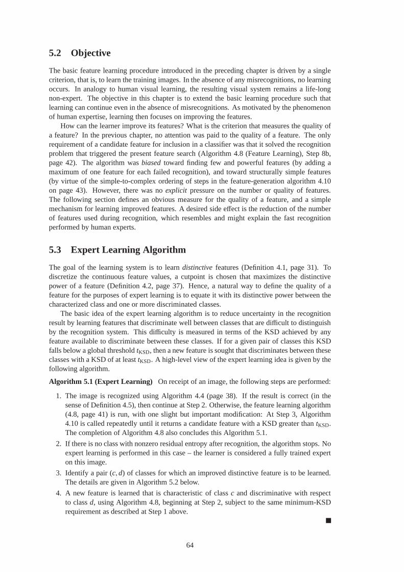
5.2 Objective

The basic feature learning procedure introduced in the preceding chapter is driven by a singlecriterion, that is, to learn the training images. In the absence of any misrecognitions, no learningoccurs. In analogy to human visual learning, the resulting visual system remains a life-longnon-expert. The objective in this chapter is to extend the basic learning procedure such thatlearning can continue even in the absence of misrecognitions. As motivated by the phenomenonof human expertise, learning then focuses on improving the features.

How can the learner improve its features? What is the criterion that measures the quality ofa feature? In the previous chapter, no attention was paid to the quality of a feature. The onlyrequirement of a candidate feature for inclusion in a classifier was that it solved the recognitionproblem that triggered the present feature search (Algorithm 4.8 (Feature Learning), Step 8b,page 42). The algorithm wasbiasedtoward finding few and powerful features (by adding amaximum of one feature for each failed recognition), and toward structurally simple features(by virtue of the simple-to-complex ordering of steps in thefeature-generation algorithm 4.10on page 43). However, there was noexplicit pressure on the number or quality of features.The following section defines an obvious measure for the quality of a feature, and a simplemechanism for learning improved features. A desired side effect is the reduction of the numberof features used during recognition, which resembles and might explain the fast recognitionperformed by human experts.

5.3 Expert Learning Algorithm

The goal of the learning system is to learndistinctive features (Definition 4.1, page 31). Todiscretize the continuous feature values, a cutpoint is chosen that maximizes the distinctivepower of a feature (Definition 4.2, page 37). Hence, a naturalway to define the quality of afeature for the purposes of expert learning is to equate it with its distinctive power between thecharacterized class and one or more discriminated classes.

The basic idea of the expert learning algorithm is to reduce uncertainty in the recognitionresult by learning features that discriminate well betweenclasses that are difficult to distinguishby the recognition system. This difficulty is measured in terms of the KSD achieved by anyfeature available to discriminate between these classes. If for a given pair of classes this KSDfalls below a global thresholdtKSD, then a new feature is sought that discriminates between theseclasses with a KSD of at leasttKSD. A high-level view of the expert learning idea is given by thefollowing algorithm.

Algorithm 5.1 (Expert Learning) On receipt of an image, the following steps are performed:

1. The image is recognized using Algorithm 4.4 (page 38). If the result is correct (in thesense of Definition 4.5), then continue at Step 2. Otherwise,the feature learning algorithm(4.8, page 41) is run, with one slight but important modification: At Step 3, Algorithm4.10 is called repeatedly until it returns a candidate feature with a KSD greater thantKSD.The completion of Algorithm 4.8 also concludes this Algorithm 5.1.

2. If there is no class with nonzero residual entropy after recognition, the algorithm stops. Noexpert learning is performed in this case – the learner is considered a fully trained experton this image.

3. Identify a pair (c, d) of classes for which an improved distinctive feature is to be learned.The details are given in Algorithm 5.2 below.

4. A new feature is learned that is characteristic of classc and discriminative with respectto classd, using Algorithm 4.8, beginning at Step 2, subject to the same minimum-KSDrequirement as described at Step 1 above.

64

A crucial part of this straightforward algorithm is Step 3. There are many ways to define a mean-ingful pair of classes that warrant learning an improved distinction. The method described inAlgorithm 5.2 below identifies a pair of classes that constitutes a “near miss” in the recognition.Hence, one of the classes is a true class (i.e., a target classpresent in the current image), andthe other is a false class. The specific pair of classes is chosen that are least well discriminatedby any feature consulted during the recognition procedure (Step 1 in Algorithm 5.1). Therefore,this is the pair of classes that would benefit the most from a better feature. Crucially, the charac-terized class of the new feature must have had nonzero residual entropy after recognition. Thisguarantees that the new feature is going to be queried next time the same training image is seen.Thus, the new feature actually improves the situation, and endless loops are avoided.

Algorithm 5.2 (Choosing a Pair of Classes for an Expert Feature) This algorithm is run atStep 3 of Algorithm 5.1, and determines a characteristic classc and a discriminated classd thatare least well discriminated by existing features:

1. For all classesci with nonzero residual entropy:

(a) If ci is a true class, then defineD as the set of all false classes; otherwise, letD be theset of all true classes.

(b) Determine the classdmini ∈ D that is least well discriminated by any feature charac-

teristic of classci , in terms of the KSDci ,dmini

. This is accomplished by computing forall classesd j ∈ D:

• Over all featuresf that are characteristic of classci , and that have been con-sulted during the recognition procedure, compute the maximum KSDci ,dj (f ). EachKSDci ,dj (f ) is computed by counting applicable instances in the instance list.

Then, the least-well discriminated classdmini is given by the feature with the weakest

value of the KSDci ,dj (f ):

KSDci ,dmini= min

dj∈Dmax

fKSDci ,dj (f )

2. The characterized and discriminated classes are given bythe pair with the weakest associ-ated KSD. Formally,c = ci andd = di , where

i = argminj

KSDcj ,dminj. (5.1)

The feature learning procedure defined by Algorithms 5.1 and5.2 attempts to learn improvedfeatures as long as there are classes with nonzero residual entropy, and as there are classes thatare discriminated at a KSD less thantKSD by any currently available feature. The thresholdtKSD

can be increased over time. There are other possible ways to learn improved features. For exam-ple, one can attempt to learn highly distinctive features between all pairs of classes exhaustively.However, this is impractical for even moderate numbers of classes, and it would likely generatea large number of features that are never going to be used in practice. A nice property of theabove algorithms is that expert feature learning – like the basic feature learning – is driven byactual experience. Successfully learned features are guaranteed to be used should the same sit-uation arise again. Thus, each new feature has a well-definedutility to the recognition system.When there is no measurable need for better features, the expert learning algorithm stops.

5.4 Experiments

Experiments were performed using the same simulated, incremental paradigm as in Section 4.5,and using the same data sets. Here, training occurred instages. The purpose of these stages was

65

to progressively increase the thresholdtKSD, below which a feature was considered weak andtriggered expert learning.

Algorithm 5.3 (Training Stages)

1. Initially, set the stage index tos= 0, and lettKSD(s) = 0.

2. Train the system by cycling through the training set, as described in Section 4.5. Cycleuntil either the training set has been learned completely (i.e., all recognitions are correct),or give up after 20 iterations. During feature learning, apply the tKSD(s) threshold asdescribed in the expert learning algorithm 5.1, Step 1.

At the end of each cycle, discard all features that have not been consulted at all during thispast cycle.

During recognition, monitor the minimum KSD encountered byAlgorithm 5.2 during thefinal iteration through the training set. This value is givenby

KSDmin(s) = minrecognitions

mini

KSDci ,dmini

where the first minimum is taken over all executions of Algorithm 5.1 during the finaliteration through the training set (cf. Equation 5.1).

3. For the next stages+ 1, set

tKSD(s+ 1) = 1−(

1− min{KSDmin(s), tKSD(s)}2

)

This rule attempts to ramp up the target KSDtKSD exponentially, asymptoting at unity, butonly if the target KSD was reached during the stage just completed, i.e. if KSDmin(s) ≥tKSD(s). If tKSD(s+ 1) > 0.98, then it was set totKSD(s+ 1) = 1.

4. Increments, and continue at Step 2.

According to this algorithm, the first stage (s= 0) is precisely the basic feature learning proce-dure used in Section 4.5. In fact, the results reported thereare those obtained after the first stageof a comprehensive training procedure, the results of whichare presented below.

5.4.1 The COIL Task

The first block of results listed in Table 5.1 corresponds to the COIL results in Table 4.2 onpage 47, but were attained after expert learning. (The ‘-inc’ tasks in Table 5.1 will be discussedin Section 5.4.4.) Most of the reported parameters are visualized for all training stages in Figure5.1. In these graphs, training stage 0 corresponds to the data in Table 4.2, and the last trainingstage corresponds to Table 5.1.

The recognition results in Table 5.1, corresponding to the top panels in Figure 5.1, indicatea dramatic performance increase. With cumulative expert training, the proportion of correctrecognitions rises by about 50% compared to the initial training stage, ignorant recognitions arereduced by about 70%, and wrong recognitions are almost eliminated. The number of ambigu-ous recognitions also increases somewhat. This is not a desired effect, but ambiguity is the bestrecognition outcome short of correctness. The accuracy reaches more than 80%, which beginsto be comparable to object recognition results reported formore specialized machine visionsystems.

Another dramatic development can be observed in the evolving feature set. The middlepanels in Figure 5.1 reveal a typical behavior. Throughout expert learning, the number of fea-tures queried during a recognition procedure decreases sharply. During Stage 1, the number of

66

Table 5.1.Summary of empirical results after expert learning on all tasks. The first four entriesgive the name of the task, the number of classes, the fold index, and the accuracy according toDefinition 4.6. The five entries under “Recognition Results”in each row sum to one, barringroundoff errors. Zero entries are left blank for clarity. The columnsunder the heading “# Fea-tures” give the total number of feature nodes in all Bayesiannetworks (BN), the total numberof different features (dif.), the average number of features queried (qu’d) during a single recog-nition procedure (Algorithm 4.4), and the total cumulativenumber of features sampled (smp’d),respectively. The rightmost two columns list the number of cycles through the training set, andthe total number of training image presentations.

Recognition Results # Features Tr. SetTask Cls. Fld. acc.cor. wrg. amb. cnf. ign.BN dif. qu’d. smp’d. cyc. imgs.

COIL 6 1 .86 .78 .02 .13 .07 10 8 6.4 19448 60 3600COIL 6 2 .78 .70 .05 .12 .13 23 17 11.1 19203 68 4080COIL 6 av. .82 .74 .03 .13 .10 17 13 8.8 19326 64 3840COIL-inc 6 1 .87 .80 .12 .08 7 6 5.5 13867 6850COIL-inc 6 2 .88 .82 .02 .10 .07 11 11 6.5 17491 11000COIL-inc 6 av. .87 .81 .01 .11 .08 9 9 6.0 15679 8925COIL-inc 10 1 .82 .77 .01 .08 .14 34 21 12.4 69450 43520COIL-inc 10 2 .80 .73 .10 .01 .16 28 16 13.0 87996 57060COIL-inc 10 av. .81 .75 .01 .09 .01 .15 31 19 12.7 78723 50290Plym 8 1 .70 .58 .06 .22 .14 23 17 8.9 33711155 8680Plym 8 2 .80 .75 .04 .09 .13 11 10 8.5 25513122 7808Plym 8 av. .75 .67 .05 .15 .13 17 14 8.7 29612139 8244Plym-inc 8 1 .77 .73 .02 .08 .17 21 11 8.2 71183 36274Plym-inc 8 2 .83 .79 .02 .05 .14 16 10 7.5 28078 15640Plym-inc 8 av. .80 .76 .02 .07 .16 19 11 7.9 49631 25957Mel 6 1 .61 .47 .03 .19 .03 .28 43 35 15.0 3766 38 1368Mel 6 2 .55 .42 .14 .22 .03 .19 26 25 8.8 13461 64 2304Mel 6 av. .58 .44 .08 .21 .03 .24 35 30 11.9 8614 51 1836Mel-inc 6 1 .64 .44 .06 .39 .11 25 22 10.4 8313 3774Mel-inc 6 2 .56 .42 .03 .17 .39 21 19 7.5 15181 3630Mel-inc 6 av. .60 .43 .04 .28 .25 23 21 9.0 11747 3702

67

0 1 2 3 40

0.2

0.4

0.6

0.8

1

0 .5 .5 .5 .75

training stages

prop

ortio

n of

test

set

COIL Fold 1

correct wrong ambiguousconfused ignorant

0 1 2 3 4 5 6 70

0.2

0.4

0.6

0.8

1

0 .5 .5 .5 .75 .88 .94 .97

training stages

prop

ortio

n of

test

set

COIL Fold 2


0 1 2 3 40

10

20

30

40

50

training stages

num

ber

of fe

atur

es

COIL Fold 1

0 1 2 3 4 5 6 70

10

20

30

40

50

60

training stages

num

ber

of fe

atur

esCOIL Fold 2

total feature nodes different features max. per recognitionmin. per recognitionavg. per recognition

0 1 2 3 40

5

10

15

20

training stages

cum

ulat

ive

num

ber

(×10

00)

COIL Fold 1

features sampledimages presented

0 1 2 3 4 5 6 70

5

10

15

20

training stages

cum

ulat

ive

num

ber

(×10

00)

COIL Fold 2


Figure 5.1.Expert Learning results on the COIL task. The numbers shown inside the top graphsgive the value oftKSD at the respective training stage. Where this number appearsin bold face,the training set was learned with perfect accuracy, and thetKSD goal was achieved. Otherwise,either the training set was not learned perfectly, or thetKSD goal was not attained. The error barsin the middle plots have a width of one standard deviation.

68

different features present in all Bayesian networks increases,eliminating most of the re-usedfeatures. This constitutes a qualitative change in the feature set, during which general featuresare replaced by more specialized, distinctive features. The total number of features is hardlyaffected (Fold 1) or is even reduced (Fold 2). During further expert learning stages, a relativelysmall number of highly distinctive features are learned, rendering a large proportion of the ex-isting features obsolete. Thus, the number of features stored by the system is reduced from 53(average over both folds) to 17. Due to the high distinctive power of the remaining features,few are queried during a recognition procedure. Fold 1 constitutes a quite drastic example: Onaverage, little more than six features are queried to recognize an image (Table 5.1). This is justone feature per class!

Figure 5.2 shows some of the expert features. Compared to thenovice features shown inFigure 4.7 on page 50, these are much more meaningful intuitively. One car is characterized bythe texture on the roof, the other by a wheel feature. Both theduck and the cat are characterizedby an eye/forehead feature. In fact, this feature is absolutely identical; it is one of the twosurviving shared features in Fold 1. Curiously, this is the only feature characteristic of a cat(Table 5.2). How can it alone suffice to characterize a cat if it is also a distinctive duck feature?The answer is that the thresholdαf for this feature to be considered present is much higher inthe cat’s Bayesian network than in the duck’s (cf. Definition4.2, Distinctive Power of a Feature,page 37). Evidently, on all duck images contained in the training set, the response valueff ofthis feature remained below the correspondingαf threshold of the cat’s network, while on all catimages, it exceeded this threshold. Otherwise, this feature alone would not have been sufficientto characterize a cat.

The confusion matrices of ambiguous recognitions is shown in Table 5.3. Some of theseambiguities are not surprising. For instance, in Fold 1 a cat(obj4) was also labeled as a duck(obj1). In both folds, the two cars (obj3 andobj6) tended to be confused. Car/car and duck/catconfusions also accounted for two of the four wrong recognitions shown in Table 5.2.

Finding highly distinctive features is not easy. The training set was first learned after a mereseven iterations (Table 5.1), during which about 700 candidate features were generated. Aftercomplete expert training, almost 20,000 features had been tried in more than 60 iterations. Asshown in the bottom panel in Figure 5.1, the bulk of this effort is spent at the first stage ofexpert learning. The reason is that initially, most of the recognitions end with a high degree ofuncertainty, and most pairwise uncertainties discovered by Algorithm 5.2 have KSDci ,dmin

i= 0.

The superior power of expert features over novice features not only results in fewer featuresqueried per recognition, but is also manifested in increased stability across viewpoints and in-creased specificity. Figure 5.3 shows all features characteristic of obj1. Remarkably, all threefeatures are present in all views except for the very last, where feature 665 is missing. Allfeatures responded reliably to corresponding object partsacross most of the viewpoint range.Figure 5.4 demonstrates the superior specificity of these expert features compared to the novicefeatures (see Figure 4.9 on page 53 for comparison). The least specific expert feature 557 re-sponds more specifically to distinct parts of the duck than the most specific novice feature 5.Even more significantly, it response on the non-duck image isweaker in most places. Fea-ture 566 acts as an eye detector – it responds to a small dark spot with a neighboring largerlight spot. As mentioned earlier, this feature is also characteristic of the cat (obj4). Feature 665detects the wing in a specific spatial relation to an outer edge of the duck object. It respondsselectively to a few locations on the duck image, but almost nowhere on the cat image.

It is quite remarkable that the learning system was able to construct such powerful features:They are specific to an object, and at the same time are generalin that they respond well over awide range of viewpoints. Interestingly, they correspond to intuitively meaningful object parts.It would not have been easy to construct such specific and yet viewpoint-invariant features byhand.

69

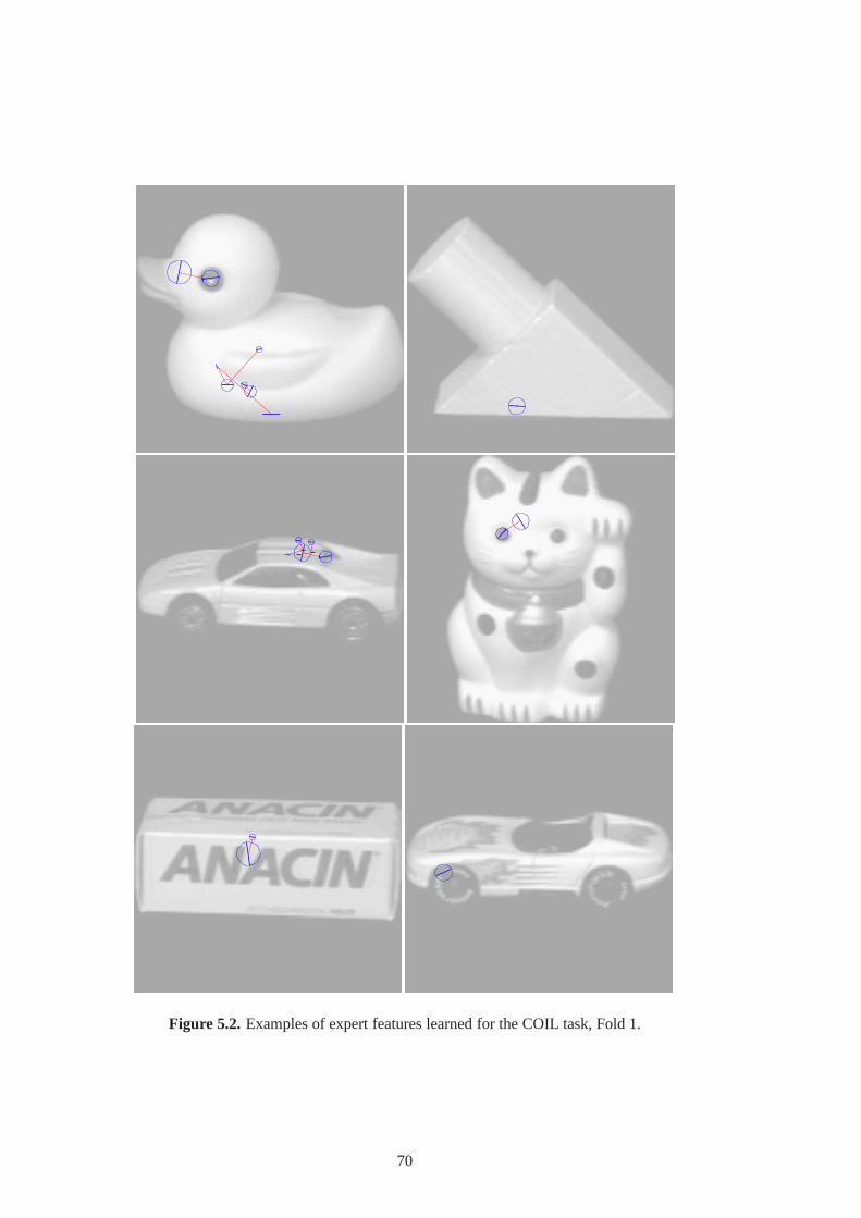
Figure 5.2. Examples of expert features learned for the COIL task, Fold 1.

70

Table 5.2. Results on the COIL task after Expert Learning. The table shows, for each class,how many instances were recognized as which class for correct and wrong recognitions, and thenumber of ambiguous/confused/ignorant recognition outcomes. In each row, these entries sumto the number of test images of each class (here, 10). The rightmost column shows the numberof feature nodes that are part of the Bayesian network representing each class. The bottom rowof the bottom panel gives the average proportion of the test set that falls into each recognitioncategory.

Confusion Matrix correct/wrong # Feats.Class obj1 obj2 obj3 obj4 obj5 obj6 amb. cnf. ign. BN

Fold 1:obj1 10 3obj2 8 2 1obj3 8 1 1 3obj4 8 2 1obj5 6 2 2 1obj6 7 1 2 1Sum 10 8 8 8 6 8 8 0 4 10

Fold 2:obj1 9 1 8obj2 8 2 2obj3 5 2 3 4obj4 1 4 1 4 1obj5 2 8 1obj6 8 2 7Sum 10 8 5 6 8 8 7 0 8 23

Average of both folds (proportions):obj1 .95 .05 6obj2 .80 .20 2obj3 .65 .05 .15 .15 4obj4 .05 .60 .15 .20 1obj5 .10 .70 .10 .10 1obj6 .75 .15 .10 4Avg. .17 .13 .11 .12 .12 .13 .13 .00 .10 3

71

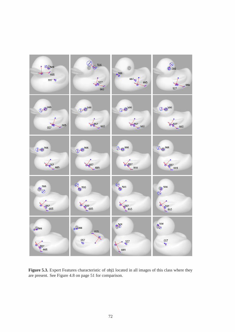
Figure 5.3. Expert Features characteristic ofobj1 located in all images of this class where theyare present. See Figure 4.8 on page 51 for comparison.

72

Figure 5.4. Spatial distribution of expert feature responses of all features characteristic ofobj1learned in Fold 1 (left columns), for comparison also shown for obj4 (right columns). In thecenter columns, the gray level encodes the response strength of the feature shown in the outerpanels. Black represents the maximal response off = 1.0; in white areas no response wascomputed. Features are labeled by their ID numbers. See Figure 4.9 on page 53 for comparison.

73

Table 5.3. Results on the COIL task after Expert Learning: Confusion matrices of ambiguousrecognitions. The italic numbers on the diagonal indicate how many times the class given on theleft was recognized ambiguously (cf. Table 5.2), and the upright numbers in each row specifythe false-positive classes.

Class obj1 obj2 obj3 obj4 obj5 obj6

Fold 1:obj1obj2 2 2obj3 1 1obj4 1 1 2obj5 2 2obj6 1 1

Fold 2:obj1obj2 1 2 1obj3 1 1 2 1obj4 1 1obj5obj6 1 1 2

The feature learning algorithm employs a random feature generation procedure (Algorithm 4.10,page 43). How sensitive is the performance of the trained system to this randomness? To givean intuition, the system was trained on Fold 1 a total of ten times, seeding the random-numbergenerator with unique values. Figure 5.5 shows the average performance of the trained novicesand experts. According to a paired-sample one-tailedt test, the superior accuracy of experts vs.novices is highly significant (p < 0.0001). There is considerable variation in the accuracies,while the number of features queried stabilizes reliably during expert learning. The reason forthis is that learning ends as soon as all recognitions leave all classifiers with zero residual en-tropy. By this time, all objects are characterized by a smallnumber of features that are highlydistinctive on the training set – however, no definitive statement can be made about their gener-alization properties to unseen test images. In realistic, open learning scenarios, this is not goingto be a problem: If an image is misrecognized or is recognizedwith less than perfect certainty,it immediately becomes a training image, and learning continues. Thus, in practice the finalperformance is expected to depend much less on the randomness intrinsic to the learner, but isdetermined by the expressiveness of the feature space.

5.4.2 The Plym Task

All of the general comments made in the previous section about the COIL task apply also tothe Plym task (Figure 5.6). As is also seen in Table 5.1 in comparison to Table 4.2, all per-formance parameters improved substantially as a result of expert learning, with the exceptionof an increased number of ambiguous recognitions. In Fold 1,progress of expert learning wasmarkedly non-monotonic. For many stages, it failed to achieve the goal oftKSD = 0.5. At theend, however, it learned the training set with a remarkabletKSD = 0.94.

Similarly to the basic learning stage,cyl6 andcucon were problematic classes (Tables 5.4and 5.5). Examples of the features learned are shown in Figure 5.7. Similarly to the COILtask, these few but highly distinctive features make much more intuitive sense than the featureslearned during the first stage (see Figure 4.11 on page 54). Notice thecon6 feature characteriz-

74

Novice Expert0

0.2

0.4

0.6

0.8

1

accu

racy

Novice Expert0

5

10

15

20

25

30

avg.

# fe

atur

es q

uerie

d pe

r re

cogn

.

Figure 5.5. Variation due to randomness in the learning procedure. The bars represent the meanperformance achieved on 10 independent learning trials of COIL-Fold 1. The error bars extendone standard deviation above and below the mean. Extrema areindicated by asterisks.

ing the converging edges, thecucon, cucy, cycu, andcyl3 features located at characteristic foldsor corners, and thetub6 feature that responds to the top rim.

What is the critical limiting factor of the performance on the Plym task, the feature space orthe learning procedure? There is no absolute answer to this question. However, if the systemcan learn to discriminate well between two particularly difficult classes if more training dataare used, then this would indicate that the limited performance is primarily an effect of thelearning procedure. A leave-one-out cross validation procedure was run on classescube andcucon. In Fold 1 of the full-scale eight-object task, these were two of the most difficult classesto recognize (Table 5.4), and in two cases acube appeared as a false positive together with acucon (Table 5.5). In Fold 2,cucon was one of the weakest classes.

Table 5.6 shows that this distinction was learned quite well, with an accuracy of 0.93. Thissuggests that the feature space is capable of expressing such distinctions. The critical limitingfactor is probably the fixed training set: Once features havebeen learned that always achieveperfect recognition with zero residual entropy, expert learning ends (cf. Section 5.3). At thisstage, the learned feature set will generally still be imperfect in that they do not fully disam-biguate all pairs of classes with a KSD of 1.0. It is features with a weak KSD and the potentialto eliminate all entropy that cause the system to fail on unseen test images. In a practical, opentask, this is not a problem because any imperfectly recognized test image automatically becomesa training image, and learning continues.

5.4.3 The Mel Task

The Mel task reflects the general phenomena observed in the COIL and Plym tasks, but to alesser extent (Figure 5.8 and Table 5.7). Contrary to this development is the slight increaseof wrong recognitions in Fold 2, and the emergence of one confused recognition in both folds(in Fold 1, anabalone board was mistaken for aphone-cord and abike-chain; in Fold 2, asock was mislabeled asgrapes and bike-chain). In Fold 2, no instances ofphone-cord wererecognized correctly, as was the case for both folds after the initial learning stage (see Table 4.7on page 58). In contrast, Fold 1 achieved some success on thisclass, but only at the expenseof 20 features dedicated to it. This is the largest number of features observed for any object inall experiments after expert learning. In fact, for both folds the number ofphone-cord featuresincreased significantly during expert learning, while it decreased for almost all other classes inall experiments.

75

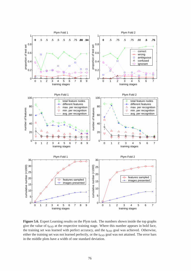
0 1 2 3 4 5 6 7 8 90

0.2

0.4

0.6

0.8

1

0 .5 .5 .5 .5 .5 .5 .75 .88 .94

training stages

prop

ortio

n of

test

set

Plym Fold 1

0 1 2 3 4 5 6 70

0.2

0.4

0.6

0.8

1

0 .5 .75 .5 .75 .88 .5 .75

training stages

prop

ortio

n of

test

set

Plym Fold 2


0 1 2 3 4 5 6 7 8 90

20

40

60

80

100

training stages

num

ber

of fe

atur

es

Plym Fold 1


0 1 2 3 4 5 6 70

20

40

60

80

100

training stages

num

ber

of fe

atur

esPlym Fold 2


0 1 2 3 4 5 6 7 8 90

5

10

15

20

25

30

35

training stages

cum

ulat

ive

num

ber

(×10

00)

Plym Fold 1


0 1 2 3 4 5 6 70

5

10

15

20

25

30

training stages

cum

ulat

ive

num

ber

(×10

00)

Plym Fold 2


Figure 5.6. Expert Learning results on the Plym task. The numbers shown inside the top graphsgive the value oftKSD at the respective training stage. Where this number appearsin bold face,the training set was learned with perfect accuracy, and thetKSD goal was achieved. Otherwise,either the training set was not learned perfectly, or thetKSD goal was not attained. The error barsin the middle plots have a width of one standard deviation.

76

Table 5.4. Results on the Plym task after Expert Learning. The table shows, for each class,how many instances were recognized as which class for correct and wrong recognitions, and thenumber of ambiguous/confused/ignorant recognition outcomes. In each row, these entries sumto the number of test images of each class (here, 8 in Fold 1 and7 in Fold 2). The rightmostcolumn shows the number of feature nodes that are part of the Bayesian network representingeach class. The bottom row of the bottom panel gives the average proportion of the test set thatfalls into each recognition category.

Confusion Matrix correct/wrong # Feats.Class con6 cube cucon cucy cycu cyl3 cyl6 tub6 amb. cnf. ign. BN

Fold 1:con6 6 2 1cube 2 2 4 7cucon 3 4 1 1cucy 4 1 2 1 1cycu 6 1 1 1cyl3 8 3cyl6 1 2 3 2 8tub6 5 3 1Sum 7 2 3 4 8 8 3 6 14 0 9 23

Fold 2:con6 7 1cube 5 1 1 4cucon 4 2 1 1cucy 6 1 1cycu 5 2 1cyl3 7 1cyl6 4 1 2 1tub6 4 1 2 1Sum 7 5 4 6 5 8 4 5 5 0 7 11

Average of both folds (proportions):con6 .87 .13 1cube .47 .07 .13 .33 6cucon .47 .40 .13 1cucy .67 .07 .13 .13 1cycu .73 .20 .07 1cyl3 1.00 2cyl6 .07 .13 .47 .07 .27 5tub6 .60 .27 .13 1Avg. .12 .06 .06 .08 .11 .13 .06 .09 .16 0 .13 2

77

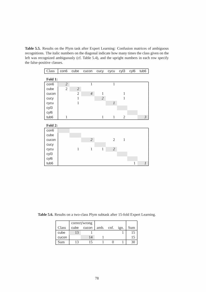
Table 5.5. Results on the Plym task after Expert Learning: Confusion matrices of ambiguousrecognitions. The italic numbers on the diagonal indicate how many times the class given on theleft was recognized ambiguously (cf. Table 5.4), and the upright numbers in each row specifythe false-positive classes.

Class con6 cube cucon cucy cycu cyl3 cyl6 tub6

Fold 1:con6 2 1 1cube 2 2cucon 2 4 1 1cucy 1 2 1cycu 1 1cyl3cyl6tub6 1 1 1 2 3

Fold 2:con6cubecucon 2 2 1cucycycu 1 1 1 2cyl3cyl6tub6 1 1

Table 5.6.Results on a two-class Plym subtask after 15-fold Expert Learning.

correct/wrongClass cube cucon amb. cnf. ign. Sumcube 13 1 1 15cucon 14 1 15Sum 13 15 1 0 1 30

78

con6 cube cucon cucy

cycu cyl3 cyl6 tub6

Figure 5.7. Examples of expert features learned for the Plym task, Fold 1.

79

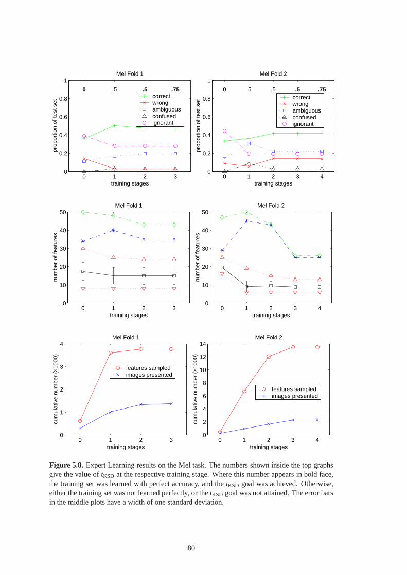
0 1 2 30

0.2

0.4

0.6

0.8

1

0 .5 .5 .75

training stages

prop

ortio

n of

test

set

Mel Fold 1


0 1 2 3 40

0.2

0.4

0.6

0.8

1

0 .5 .5 .5 .75

training stages

prop

ortio

n of

test

set

Mel Fold 2


0 1 2 30

10

20

30

40

50

training stages

num

ber

of fe

atur

es

Mel Fold 1

0 1 2 3 40

10

20

30

40

50

training stages

num

ber

of fe

atur

es

Mel Fold 2

0 1 2 30

1

2

3

4

training stages

cum

ulat

ive

num

ber

(×10

00)

Mel Fold 1


0 1 2 3 40

2

4

6

8

10

12

14

training stages

cum

ulat

ive

num

ber

(×10

00)

Mel Fold 2


Figure 5.8. Expert Learning results on the Mel task. The numbers shown inside the top graphsgive the value oftKSD at the respective training stage. Where this number appearsin bold face,the training set was learned with perfect accuracy, and thetKSD goal was achieved. Otherwise,either the training set was not learned perfectly, or thetKSD goal was not attained. The error barsin the middle plots have a width of one standard deviation.

80

Table 5.7. Results on the Mel task after Expert Learning. The table shows, for each class,how many instances were recognized as which class for correct and wrong recognitions, and thenumber of ambiguous/confused/ignorant recognition outcomes. In each row, these entries sumto the number of test images of each class (here, 6). The rightmost column shows the numberof feature nodes that are part of the Bayesian network representing each class. The bottom rowof the bottom panel gives the average proportion of the test set that falls into each recognitioncategory.

Confusion Matrix correct/wrong # Feats.Class abalone chain grapes necktie cord sock amb.cnf. ign. BN

Fold 1:abalone 2 2 1 1 5bike-chain 3 3 7grapes 1 1 4 7necktie 2 2 2 1phone-cord 4 2 20sock 5 1 3Sum 2 3 1 2 4 6 7 1 10 43

Fold 2:abalone 3 1 2 1bike-chain 1 1 2 2 1grapes 4 2 8necktie 4 2 1phone-cord 3 3 14sock 3 1 2 1Sum 3 1 7 5 0 4 8 1 7 26

Average of both folds (proportions):abalone .42 .08 .33 .08 .08 3bike-chain .33 .08 .42 .17 4grapes .42 .08 .17 .33 8necktie .50 .33 .17 1phone-cord .25 .33 .42 17sock .67 .08 .25 2Avg. .07 .06 .11 .10 .06 .14 .21 .03 .24 6

81

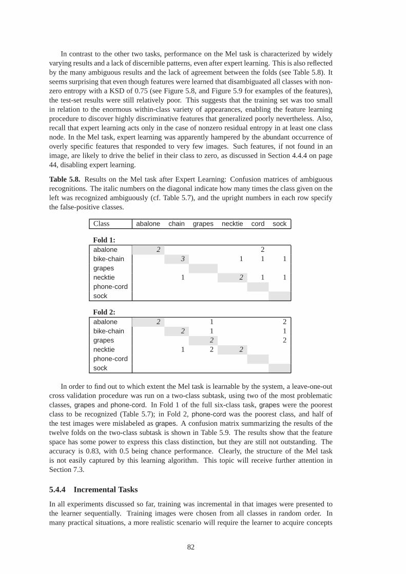
In contrast to the other two tasks, performance on the Mel task is characterized by widelyvarying results and a lack of discernible patterns, even after expert learning. This is also reflectedby the many ambiguous results and the lack of agreement between the folds (see Table 5.8). Itseems surprising that even though features were learned that disambiguated all classes with non-zero entropy with a KSD of 0.75 (see Figure 5.8, and Figure 5.9for examples of the features),the test-set results were still relatively poor. This suggests that the training set was too smallin relation to the enormous within-class variety of appearances, enabling the feature learningprocedure to discover highly discriminative features thatgeneralized poorly nevertheless. Also,recall that expert learning acts only in the case of nonzero residual entropy in at least one classnode. In the Mel task, expert learning was apparently hampered by the abundant occurrence ofoverly specific features that responded to very few images. Such features, if not found in animage, are likely to drive the belief in their class to zero, as discussed in Section 4.4.4 on page44, disabling expert learning.

Table 5.8. Results on the Mel task after Expert Learning: Confusion matrices of ambiguousrecognitions. The italic numbers on the diagonal indicate how many times the class given on theleft was recognized ambiguously (cf. Table 5.7), and the upright numbers in each row specifythe false-positive classes.

Class abalone chain grapes necktie cord sock

Fold 1:abalone 2 2bike-chain 3 1 1 1grapesnecktie 1 2 1 1phone-cordsock

Fold 2:abalone 2 1 2bike-chain 2 1 1grapes 2 2necktie 1 2 2phone-cordsock

In order to find out to which extent the Mel task is learnable bythe system, a leave-one-outcross validation procedure was run on a two-class subtask, using two of the most problematicclasses,grapes andphone-cord. In Fold 1 of the full six-class task,grapes were the poorestclass to be recognized (Table 5.7); in Fold 2,phone-cord was the poorest class, and half ofthe test images were mislabeled asgrapes. A confusion matrix summarizing the results of thetwelve folds on the two-class subtask is shown in Table 5.9. The results show that the featurespace has some power to express this class distinction, but they are still not outstanding. Theaccuracy is 0.83, with 0.5 being chance performance. Clearly, the structure of the Mel taskis not easily captured by this learning algorithm. This topic will receive further attention inSection 7.3.

5.4.4 Incremental Tasks

In all experiments discussed so far, training was incremental in that images were presented tothe learner sequentially. Training images were chosen fromall classes in random order. Inmany practical situations, a more realistic scenario will require the learner to acquire concepts

82

Figure 5.9. Examples of expert features learned for the Mel task, Fold 1.

Table 5.9.Results on a two-class Mel subtask after 12-fold Expert Learning.

correct/wrongClass grapes cord amb. cnf. ign. Sumgrapes 9 2 1 12phone-cord 1 8 1 2 12Sum 10 8 3 0 3 24

83

sequentially. In particular, this is how humans are taught.It helps us to master skills if we learnonly a limited number of them in parallel. In this section, tasks are presented to the learnerincrementally, as described in the following algorithm.

Algorithm 5.4 (Incremental Task) To train the learning system on an incremental task, beginwith a blank-slate learner, and then perform the following steps.

1. Create a training set consisting of all training images ofthe first two classes.

2. Train the system using Algorithm 5.3, with one minor modification: At Step 4, stop aftera maximum of 10 stages of expert learning.

3. If there are untaught classes, then add all training images of the next untaught class to thetraining set, and continue with Step 2. Otherwise, stop.

Importantly, the experience of the learner is not discardedbetween executions of Step 2.

The results achieved on the three tasks using Algorithm 5.4 are included in Table 5.1, with‘-inc’ appended to the task name. Interestingly, in all cases the achieved accuracy was slightlybetter than in the corresponding non-incremental tasks. Moreover, the number of features sam-pled – which is closely related to the overall running time ofthe system – is slightly reducedfor the COIL task. The number of cycles through the training set is not given in Table 5.1. Ithas little meaning for incremental tasks, as the size of the training set increases over time. Thenumber of training image presentations is drastically increased. The reason for this is that thegrowing number of already-learned images is included with every cycle, while learning concen-trates primarily on images of the new class. This effect can be avoided by more sophisticatedincremental learning schemes. For example, the simulated environment could choose the classof a training image according to the empirical misrecognition rate attained by the learner. In anycase, the choice of a learning strategy depends on the interaction dynamics between the learnerand its environment. An environment or a task may or may not allow the learner to influencethe distribution of training images.

The COIL-inc task was continued up to a total of 10 classes, which are illustrated in Figure5.10. Figures 5.11 and 5.12 show performance parameters on atest set as they evolve duringincremental expert training. The test set contains the sameclasses as the training set. Usually,the introduction of a new class causes a temporary drop in performance that is reflected bymost performance parameters: The proportion of correct recognitions drops, while most of theother parameters increase. Over the next few stages of expert training, the system recovers.Importantly, the transient drops in performance co-occur with an imperfectly learned trainingset, as indicated by the non-bold KSD indicators in Figures 5.11 and 5.12. In other words,good performance on the training images generally predictsgood performance on unseen testimages. This is good news, given the often non-monotonic performance improvement duringexpert learning. Nevertheless, a slight drop in accuracy isnoticeable, as the number of classesincreases.

How difficult are individual classes to learn? There is no way to answer this question forthe non-incremental version of expert training. However, incremental training lends insight intoa related question: How much effort does it take to learn a new class, after having learnedsome other classes? Figure 5.13 reveals that some classes are learned after sampling only asmall number of features, while others require a lot of sampling effort. Both folds learned thefirst four objects quite effortlessly, whileobj7 andobj8 were more difficult. Interestingly, bothfolds spent most effort disambiguatingobj7 from obj2 – these are the two wooden blocks in thedata set. In addition, Fold 1 often confusedobj7 with obj6, possibly due to the striped textureshared by both objects. In the case ofobj8, there was no such singular source of confusion.Nevertheless, the two classes that accounted by far for mostconfusions wereobj1 and obj6.Almost all confusions on the training set that occurred at any time during learning involved the

84

obj1 obj2 obj3 obj4 obj5

obj6 obj7 obj8 obj9 obj10

Figure 5.10.Objects used in the 10-object COIL task.

most recently introduced class, especially during the early stages of expert learning. Beyondthese qualitative remarks, it is difficult to draw strong conclusions from only two folds of crossvalidation, and from a single presentation order of new classes.

The number of expert learning stages taken until a class was learned is clearly correlatedwith the number of features sampled. However, it is not as reliable an indicator of class difficulty,because – in contrast to the number of features sampled – it islargely unrelated to the proportionof difficult training images of a class. A single difficult image can stretch expert learning overmany stages, but far fewer features are sampled than in the case of many difficult images. Forexample, in Fold 1, forobj6 11,470 features were sampled during 4 stages, whereas forobj10only 5,760 features were sampled during 9 stages.

The results for the incremental Plym task (Figures 5.14, 5.15 and 5.16) show the samecharacteristics as the COIL-inc task. Here, both folds agree thattub6, the eighth class, is themost difficult class (Figure 5.16). Not surprisingly, confusions with cyl6 accounted for theoverwhelming majority of the feature learning efforts. Notably, Fold 1 had trouble with a fewindividual images while learning the sixth and seventh classes (cyl3 andcyl6). At almost all ofthese stages, Algorithm 5.3 at Step 2 cycled through the training set the maximum of 20 times,while sampling very few features.

The Mel-inc results again show similar behavior, but to a lesser extent (Figures 5.17 and5.18). These graphs reflect the same variability as discussed for the other Mel experimentsabove. In contrast to the COIL and Plym tasks, it appears thatthe number of features sampledgrows purely as a function of the number of classes. This is another indicator of the intrinsicdifficulty of the Mel data set, which makes it hard for the learningprocedure to find powerfuland well-generalizing features. Interestingly, while learning the fourth class (necktie) in Fold 2,only 69 features were sampled, all of them during Stage 0. Thefollowing four stages of expertlearning only re-estimated the conditional probabilitiesin the Bayesian networks, but neverrequired a new feature.

In both folds, the system failed to recover after the introduction of the sixth class (sock).This is somewhat surprising, given that this class performed better than any other class after non-incremental training (Table 5.7), and is yet another indicator that expert learning was severelyhampered on the Mel task. Expert learning essentially failed here because a large number ofoverly specialized features caused most recognitions to result in zero entropy in all class nodes.Such an effect is only likely to occur on static, small, and heterogeneous training sets such asthat used in the Mel task.

85

2 3 4 5 6 7 8 9 10 0

0.2

0.4

0.6

0.8

1

0 .5 .75 .88 0 .5 .75 0 .5 .75 0 .5 .75 .88 .94 .97 0 .5 .75 .88 0 .5 .75 .88 .94 .97 1 1 0 .5 .75 .5 .5 .75 .5 .75 .5 .5 .75 0 .5 .5 .5 .75 0 .5 .75 .88 .94 .97 .5 .75 .88

number of classes

prop

ortio

n of

test

set

COIL−inc Fold 1


2 3 4 5 6 7 8 9 10 0

10

20

30

40

50

number of classes

num

ber

of fe

atur

es

COIL−inc Fold 1


Figure 5.11. Incremental Expert Learning results on the COIL-inc task, Fold 1. The vertical dotted lines indicate the addition of a new class to the trainingset. Below the graphs, these are annotated with the total number of classes represented in the training set. Data points between these lines correspond to expertlearning stages (cf. Figure 5.1, page 68), which are not numbered here. The numbers inside the top graph indicate the values oftKSD as in Figure 5.1.

86

2 3 4 5 6 7 8 9 10 0

0.2

0.4

0.6

0.8

1

0 .5 0 .5 .75.88 0 .5 .75.88.94.97 1 1 0 .5 .5 .75 .5 .5 .75.88 0 .5 .5 .75.88 0 .5 .75 .5 .75.88 0 .5 .5 .5 .75.88 .5 .5 .5 .5 .75 0 .5 .75.88.94.97 0 .5 .5 .75.88.94 .5 .75 .5 .75.88

number of classes

prop

ortio

n of

test

set

COIL−inc Fold 2


2 3 4 5 6 7 8 9 10 0

10

20

30

40

50

60

70

number of classes

num

ber

of fe

atur

es

COIL−inc Fold 2


Figure 5.12. Incremental Expert Learning results on the COIL-inc task, Fold 2. The vertical dotted lines indicate the addition of a new class to the trainingset. Below the graphs, these are annotated with the total number of classes represented in the training set. Data points between these lines correspond to expertlearning stages that are not numbered here. The numbers inside the top graph indicate the values oftKSD.

87

2 3 4 5 6 7 8 9 10 0

10

20

30

40

50

60

70

number of classes

cum

ulat

ive

num

ber

(×10

00)

COIL−inc Fold 1


2 3 4 5 6 7 8 9 10 0

20

40

60

80

100

number of classes

cum

ulat

ive

num

ber

(×10

00)

COIL−inc Fold 2


Figure 5.13.Numbers of features sampled during the COIL-inc task.

88

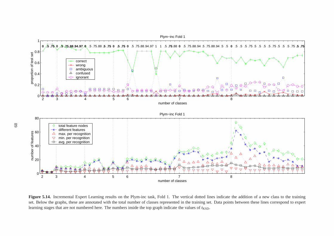
2 3 4 5 6 7 8 0

0.2

0.4

0.6

0.8

1

0 .5 .75 0 .5 .75.88.94.97 0 .5 .75.88 .5 .75 0 .5 .75 0 .5 .75.88.94.97 1 1 .5 .75 .88 0 .5 .75.88.94 .5 .75.88.94 .5 .5 0 .5 .5 .5 .75 .5 .5 .5 .5 .75 .5 .5 .5 .75 .5 .75

number of classes

prop

ortio

n of

test

set

Plym−inc Fold 1


2 3 4 5 6 7 8 0

20

40

60

80

number of classes

num

ber

of fe

atur

es

Plym−inc Fold 1


Figure 5.14. Incremental Expert Learning results on the Plym-inc task, Fold 1. The vertical dotted lines indicate the addition of a new class to the trainingset. Below the graphs, these are annotated with the total number of classes represented in the training set. Data points between these lines correspond to expertlearning stages that are not numbered here. The numbers inside the top graph indicate the values oftKSD.

89

2 3 4 5 6 7 8 0

0.2

0.4

0.6

0.8

1

0 .5 .75 0 .5 .75 0 .5 .75 .88 .94 0 .5 .75 0 .5 .75 .88 0 .5 .75 0 .5 .75 .88 .5 .75 .88 .94 .97 1

number of classes

prop

ortio

n of

test

set

Plym−inc Fold 2


2 3 4 5 6 7 8 0

10

20

30

40

50

number of classes

num

ber

of fe

atur

es

Plym−inc Fold 2


Figure 5.15. Incremental Expert Learning results on the Plym-inc task, Fold 2. The vertical dotted lines indicate the addition of a new class to the trainingset. Below the graphs, these are annotated with the total number of classes represented in the training set. Data points between these lines correspond to expertlearning stages that are not numbered here. The numbers inside the top graph indicate the values oftKSD.

90

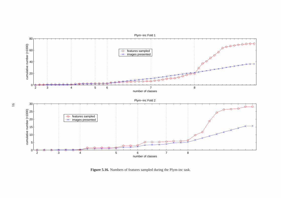
2 3 4 5 6 7 8 0

20

40

60

80

number of classes

cum

ulat

ive

num

ber

(×10

00)

Plym−inc Fold 1


2 3 4 5 6 7 8 0

5

10

15

20

25

30

number of classes

cum

ulat

ive

num

ber

(×10

00)

Plym−inc Fold 2


Figure 5.16.Numbers of features sampled during the Plym-inc task.

91

2 3 4 5 6 0

0.2

0.4

0.6

0.8

1

0 .5 .75 0 .5 .75 0 .5 .75 .88 .94 0 .5 .75 .88 0 .5 .75 .88

number of classes

prop

ortio

n of

test

set

Mel−inc Fold 1

2 3 4 5 6 0

10

20

30

40

50

number of classes

num

ber

of fe

atur

es

Mel−inc Fold 1


2 3 4 5 6 0

2

4

6

8

10

number of classes

cum

ulat

ive

num

ber

(×10

00)

Mel−inc Fold 1


Figure 5.17. Incremental Expert Learning results on the Mel-inc task, Fold 1. The verticaldotted lines indicate the addition of a new class to the training set. Below the graphs, these areannotated with the total number of classes represented in the training set. Data points betweenthese lines correspond to expert learning stages that are not numbered here. The numbers insidethe top graph indicate the values oftKSD.

92

2 3 4 5 6 0

0.2

0.4

0.6

0.8

1

0 .5 .75 0 .5 .75 0 .5 .75 .88 .94 0 .5 .5 .75 0 .5 .5 .75

number of classes

prop

ortio

n of

test

set

Mel−inc Fold 2


2 3 4 5 6 0

10

20

30

40

50

number of classes

num

ber

of fe

atur

es

Mel−inc Fold 2


2 3 4 5 6 0

5

10

15

20

number of classes

cum

ulat

ive

num

ber

(×10

00)

Mel−inc Fold 2


Figure 5.18. Incremental Expert Learning results on the Mel-inc task, Fold 2. The verticaldotted lines indicate the addition of a new class to the training set. Below the graphs, these areannotated with the total number of classes represented in the training set. Data points betweenthese lines correspond to expert learning stages that are not numbered here. The numbers insidethe top graph indicate the values oftKSD.

93

5.4.5 Computational Demands

The current method attempts to find features by random sampling in image space, which isguided by a set of simple-to-complex heuristics defined by the feature generation algorithm 4.10(page 43). Highly distinctive features are rare and difficult to find, as illustrated by the graphs inthis chapter. This opens up the question of computational demands. The current MATLABTM

implementation of the learning system takes many days of computation on a 700 MHz Pen-tium III processor to learn a typical task. The bulk of this time is spent measuring the value offeatures in images (Equation 3.14 on page 25). This is the primary reason why the extractionof salient points is so important (Section 3.4.3, page 21). For every featuref sampled, its valueff (I ) must be computed on 2nex example images (Algorithm 4.8, Feature Learning, page 41,Steps 2 and 5).

Given the number of pixels in an image (16,384 for the COIL images, 76,800 for the Melimages) and the infinite combinatorics opened up by the feature space, sampling 10,000 or100,000 features to solve a task involving 100 training images does not seem outrageous. Whatwould it take to run the feature learning algorithms on massively parallel neural hardware?Computing feature values is a pixel-level parallel operation that can plausibly be performed bythe human visual cortex. Such a parallel implementation could measure a feature value in animage in constant time, independent of the number of salientpoints in an image. Assuming anaverage of 1,000 salient points in an image, and assuming that 99% of the compute time is spentcomputing feature values, this would reduce the time to solve a reasonably large problem from,say, 10 days to less than 2 hours 40 minutes – about two orders of magnitude.

The above argument assumes that the time spent to compute a feature value is approximatelyconstant. This is not strictly true, as it depends on the length of a response vector, which is 15filter responses for texels and 2 for edgels. It also depends on the local scale of a feature and itssubfeatures, which determines the size of the filter kernelsused in Algorithm 3.6 (Extraction ofa Geometric-Compound Feature Response Vector, page 26) at Steps 1 and 4. This size variesfrom about 25 coefficients up to about 1/16 the size of the image. The early visual cortex extractssuch response vectors in parallel, for all image locations,over a range of scales, reducing thiscomputation to constant time. If these factors are taken into account, the computation time canbe reduced by at least two more orders of magnitude.

In summary, the computational demands of the expert learning procedure limit the size ofthe problems that can be addressed using today’s conventional computing hardware. However,a biologically plausible implementation that exploits thehigh degree of inherent parallelismshould reduce the computational demands by about four orders of magnitude. In principle, thiswould permit much larger-scale applications.

With respect to scalability, an important consideration isthe number of distinctions that hasto be learned by the system. In general, this number is quadratic in the number of classes: Eachclass is to be discriminated from each of the other classes. Figure 5.19 plots the cumulativenumber of features sampled in the incremental tasks versus the number of classes. Clearly, thegrowth is superlinear. However, there are not sufficient data to allow a conclusive statementregarding the complexity of the learning algorithm with respect to the number of classes. Moreexperiments using more classes are required. In any case, this superlinear growth is likely tolimit the maximal problem size that can be addressed by this system. However, this need notconstitute a practical limitation. Humans clearly do not learn expert-level distinctions betweenall categories that have any meaning to them in any context. Rather, at any given time, thebehavioral context constrains the relevant categories to arelatively small set. Expert learning isonly required where distinctions need to be refined that are relevant within a given context.

94

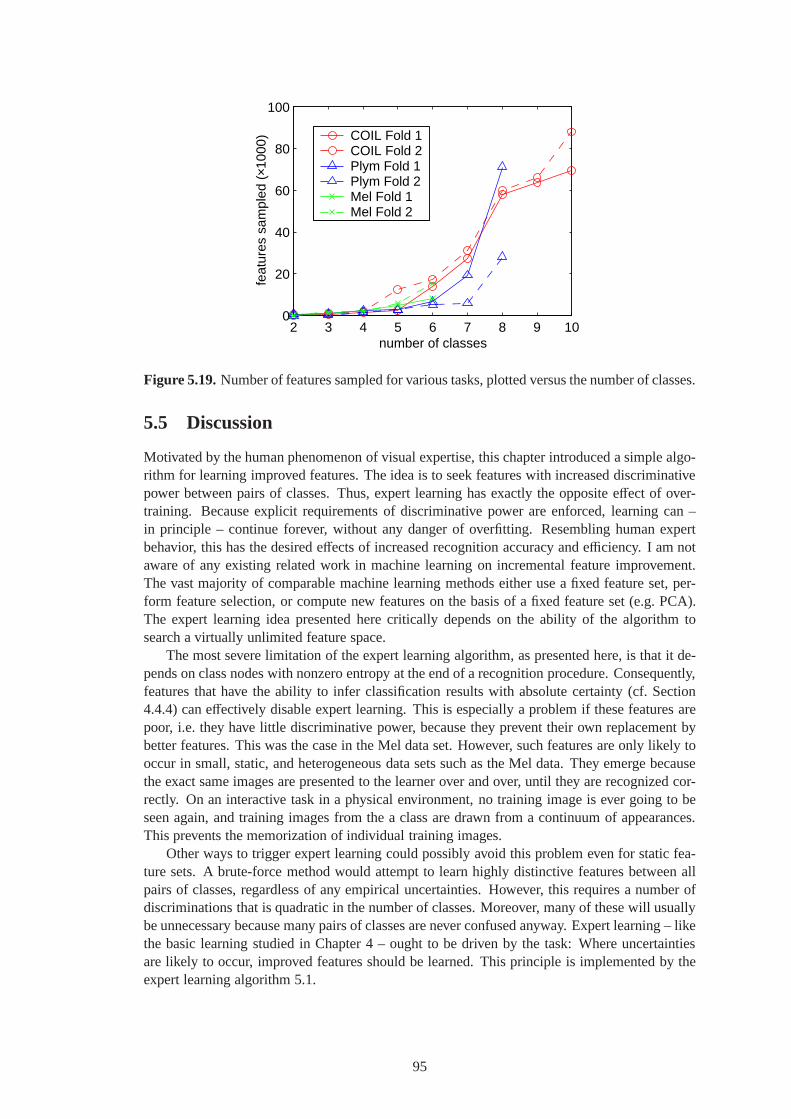
2 3 4 5 6 7 8 9 100

20

40

60

80

100

number of classes

feat

ures

sam

pled

(×1

000) COIL Fold 1

COIL Fold 2Plym Fold 1Plym Fold 2Mel Fold 1 Mel Fold 2

Figure 5.19.Number of features sampled for various tasks, plotted versus the number of classes.

5.5 Discussion

Motivated by the human phenomenon of visual expertise, thischapter introduced a simple algo-rithm for learning improved features. The idea is to seek features with increased discriminativepower between pairs of classes. Thus, expert learning has exactly the opposite effect of over-training. Because explicit requirements of discriminative power are enforced, learning can –in principle – continue forever, without any danger of overfitting. Resembling human expertbehavior, this has the desired effects of increased recognition accuracy and efficiency. I am notaware of any existing related work in machine learning on incremental feature improvement.The vast majority of comparable machine learning methods either use a fixed feature set, per-form feature selection, or compute new features on the basisof a fixed feature set (e.g. PCA).The expert learning idea presented here critically dependson the ability of the algorithm tosearch a virtually unlimited feature space.

The most severe limitation of the expert learning algorithm, as presented here, is that it de-pends on class nodes with nonzero entropy at the end of a recognition procedure. Consequently,features that have the ability to infer classification results with absolute certainty (cf. Section4.4.4) can effectively disable expert learning. This is especially a problem if these features arepoor, i.e. they have little discriminative power, because they prevent their own replacement bybetter features. This was the case in the Mel data set. However, such features are only likely tooccur in small, static, and heterogeneous data sets such as the Mel data. They emerge becausethe exact same images are presented to the learner over and over, until they are recognized cor-rectly. On an interactive task in a physical environment, notraining image is ever going to beseen again, and training images from the a class are drawn from a continuum of appearances.This prevents the memorization of individual training images.

Other ways to trigger expert learning could possibly avoid this problem even for static fea-ture sets. A brute-force method would attempt to learn highly distinctive features between allpairs of classes, regardless of any empirical uncertainties. However, this requires a number ofdiscriminations that is quadratic in the number of classes.Moreover, many of these will usuallybe unnecessary because many pairs of classes are never confused anyway. Expert learning – likethe basic learning studied in Chapter 4 – ought to be driven bythe task: Where uncertaintiesare likely to occur, improved features should be learned. This principle is implemented by theexpert learning algorithm 5.1.

95

CHAPTER 6

LEARNING FEATURES FOR GRASP PRE-SHAPING

The preceding chapters applied feature learning in a supervised object recognition scenario.Many of the visual skills that humans acquire from experience affect their behavior at a veryfine granularity. For example, between about five to nine months of age, infants learn to pre-orient their hands to match the orientation of a target object during reaching [70]. In this chapter,visual features are learned that enable similar prospective behavior in a haptically-guided roboticgrasping system.

6.1 Related Work

There is extensive literature on visual servoing; a thorough review is beyond the scope of thisdissertation. Most of this work falls into one of two main categories according to the coordinateframe in which error signals are computed, namely, three-dimensional workspace coordinates ortwo-dimensional image coordinates. Three-dimensional methods typically rely on a reasonablycomplete and accurate visual reconstruction of the workspace. More related to this chapterare two-dimensional approaches where manipulator controlsignals are directly derived fromimage-space errors [105, 49]. Here, local features of the manipulator and of workpieces areidentified, and their actual positions are compared to reference positions. Image-space errorsare then transformed into errors in the degrees of freedom ofthe manipulator. Instead of localappearance, another line of research builds on global appearance and computes error signals ineigen-subspaces [74].

6.2 Objective

To date, most work in sensor-guided robotic manipulation has concentrated on exclusivelyvision-based systems. There has been much less work on haptically-guided grasping [21, 23],or on combining haptic and visual feedback [3, 42]. This seems somewhat surprising, as thesetwo sensory modalities ideally complement each other, especially when a dextrous manipulatoris used. The visual system is most beneficial during the reachphase when no haptic feedback isavailable. Relatively coarse differential error signals in image space, using appearance featuresof the wrist or the arm, are sufficient to achieve a highly efficient vision-guided reach. Whenthe end effector draws close to the target object, visual information can further contribute tothe extent that fingertips and object details are accuratelyidentified. However, this is difficultto achieve because these features will often be occluded by the hand itself. Moreover, even ifdetailed information about finger configurations can be obtained by the vision system, it will bedifficult to exploit in the context of a dextrous manipulator due to the many degrees of freedominvolved, many of which are redundant. This stage of the grasp is ideally suited for haptic feed-back. Tactile fingertip sensors are highly sensitive to relevant surface characteristics such as theorientation of the local surface tangent. Coelho [21, 23] has demonstrated that this informationcan be exploited by local grasp controllers that converge toward stable grasp configurations,thereby obviating the need to solve a high-dimensional (andoften intractable) planning problemin global joint space.

97

McCarty et al. [70] demonstrated that infants learn to pre-orient their hand during a reachto match the orientation of the target object. Notably, thisprospective behavior does not dependon the visibility of the hand or of the object during the reach. Evidently, humans use an initialvisual cue to initiate a reach, that is then guided by proprioception. Once the target object iscontacted, the grasp is completed using tactile feedback.

Coelho’s closed-loop grasping system is “blind” in the sense that no visual information isexploited during the grasp process. The objective in this chapter is to add a visual componentto this system that extracts minimal visual information to pre-orient the hand appropriately inrelation to the target object. Specifically, it recommends two critical parameters to the hapticsystem:

• the orientation (azimuthal angle) of the hand, and

• the number of fingers to use (two or three).

These recommendations are purely based on features of appearance that correlate robustly withthese two parameters, using a feature learning system similar to that discussed in the precedingchapters. The learning procedure is driven entirely by the haptic grasping system, without anexternal supervisor.

6.3 Background

The grasping task discussed in this chapter is based on a haptically-guided grasping systemdeveloped by my colleague Jefferson Coelho, which is introduced in the next section. Then,Section 6.3.2 briefly introduces and illustrates probability distributions on angular domains.These play an important role in the algorithms presented in this chapter.

6.3.1 Haptically-Guided Grasping

Coelho [21] describes a framework for closed-loop graspingusing a dextrous robotic hand (Fig-ure 6.1) equipped with force/torque touch sensors at the fingertips. Reference and feedbackerror signals are expressed in terms of the object-framewrench residualρ, a six-element vectorsummarizing the residual forces and torques acting on the object. The current object wrenchis computed using the instantaneous grip JacobianG, which in turn is locally estimated usingsensor feedback in the form of contact positions and normals. The grasp controllerπ receives anerror signalǫ, which for a zero reference wrench is simply the squared wrench residualǫ = ρTρ,and computes incremental displacements for a subset of the fingertip contacts so as to reduce theerror signal. As a result, the fingers probe the surface of theobject until their positions convergeto a local minimum in the squared-wrench-residual surface.

G

Controlactions

GraspController

Contact normalsand positions

Σ

Plant

Objectwrench

Referencewrench

Figure 6.1. Grasp synthesis as closed-loop control. (Reproduced with permission from Coelhoand Grupen [21].)

98

The three-fingered Stanford/JPL robotic hand (Figure 6.2) employed in this work can per-form grasps using any two- or three-fingered grasp configuration. Each of these finger combina-tionsc gives rise to an individual grasp controllerπc, yielding a total of four controllers. For thepurpose of this chapter, it is sufficient to distinguish between two classes of grasp controllers,namely, two- and three-fingered grasps.

Figure 6.2. The Stanford/JPL dextrous hand performing haptically-guided closed-loop graspsynthesis.

As a grasp controllerπc executes, the control errorǫ and its time derivative ˙ǫ trace out phaseportraits that are characteristic of object shapes (Figure6.3). In this way, the grasping systemforms haptic categories. Qualitatively different regions in a phase portrait constitute hapticcontextsand can be represented as states of a finite state machine (Figure 6.4). Coelho [22, 23]describes a reinforcement learning framework for learninggrasp control policies that select acontrollerπc based on the context currently observed. The learned policies achieve grasps ofconsistently higher quality than any fixednativecontrollerπc by escaping local minima in thewrench residual surface.

ε

ε

0.2 0.4

−0.010

−0.005

(a)

(b)

(c)

(c)

(b)

(a)

ε

ε0.2 0.4 0.6 0.8

−0.020

−0.015

−0.010

−0.005

µ = 1.320

µ = 0.280

µ = 0.680

Figure 6.3. Object wrench phase portraits traced during grasp syntheses. The left panel depictsthe evolution of a two fingered grasp trial from configuration(a) to (b) and to (c), the convergentconfiguration. The complete, two-fingered phase portrait for the irregular triangle is shown onthe right. (Reproduced with permission from Coelho et al. [24])

99

ε ε

A

B

CD

E

π

B

A

C

D E

A,B

B,C

A,CB,D,E

D,E

ιPolicy

Figure 6.4. A hypothetical phase portrait of a native controllerπc (left) and all possible contexttransitions (right). (Reproduced with permission from Coelho et al. [24])

The quality of a grasp is characterized by the minimum friction coefficientµ0 required for anull space to exist in the grip JacobianG, with rank≥ 1. For an ideal grasp,µ0 = 0, meaningthat the grasp configuration is suitable for fixing the objectin place using frictionless pointcontacts. Depending on the object shape and the number of fingers available, this ideal may notbe achievable. The right panel in Figure 6.3 is annotated with the values ofµ0 associated withthe three converged configurations.

6.3.2 The von Mises Distribution

Predicting hand orientations in relation to objects involves the estimation of relative angularinformation. Most conventional continuous probability distributions have a linear domain, forexample, the normal distribution. In the case where a randomvariable represents an angle, oneprobability distribution that is often used in lieu of a normal distribution on a circular domain isthevon Misesdistribution [30]. It has the probability density function

pvM(θ | µ, κ) = 12πI0(κ)

eκ cos(θ−µ) (6.1)

where 0≤ µ < 2π, 0 ≤ κ < ∞, and I0(κ) is the modified Bessel function of order zero. Themean direction of the distribution is given byµ, andκ is a concentration parameter withκ = 0corresponding to a circular uniform distribution, andκ → ∞ to a point distribution. Figure 6.5illustrates four von Mises distributions with different parameters. The probability density at anangle corresponds to the radial distance from the unit circle to the density curve.

The parameterµ of the von Mises distribution is not to be confused with the friction coef-ficient µ0 introduced in the previous section. I use this notation in agreement with establishedconventions. In this chapter, the use ofµ is consistent:µ0 (occasionally followed by one moreindex) always refers to the friction coefficient, andµ (often with an index other than zero) alwaysdenotes the mean direction of a von Mises distribution.

6.4 Feature Learning

In Coelho’s haptically-guided grasping system, no visual cues guide the placement of the fingerson the object. Here, the goal is to learn visual features thatpredict successful hand orientations,

100

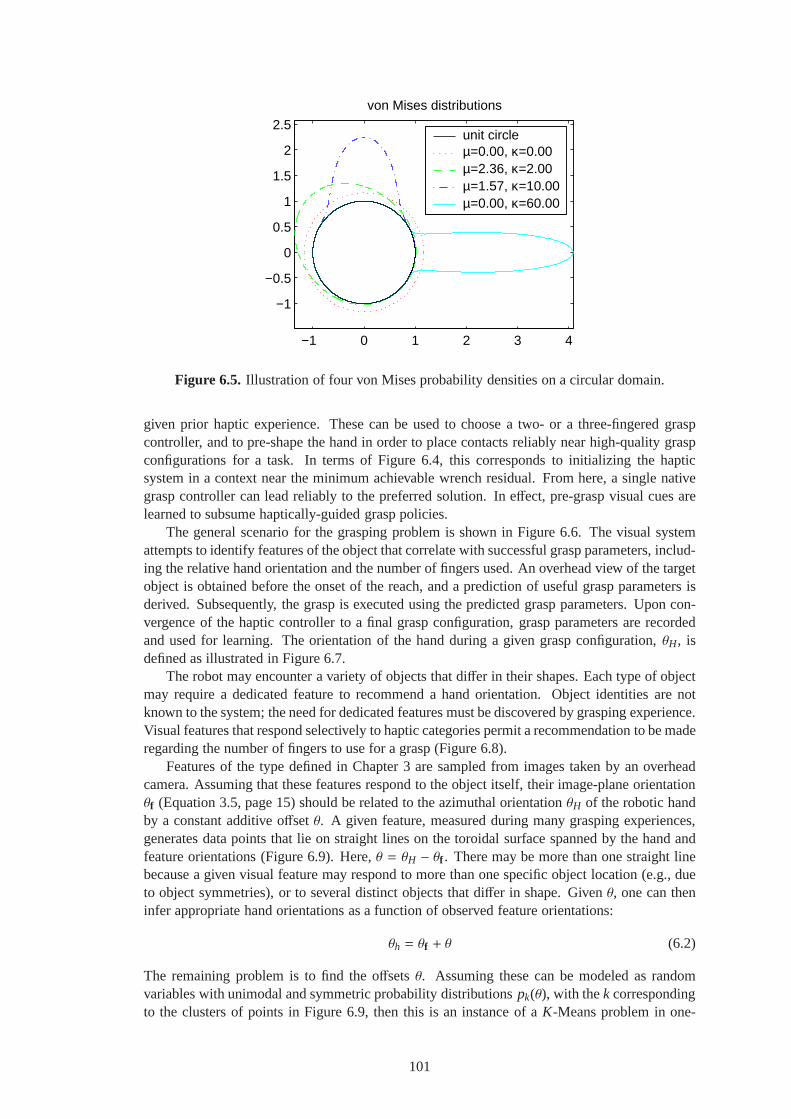
−1 0 1 2 3 4

−1

−0.5

0

0.5

1

1.5

2

2.5

von Mises distributions

unit circle µ=0.00, κ=0.00 µ=2.36, κ=2.00 µ=1.57, κ=10.00µ=0.00, κ=60.00

Figure 6.5. Illustration of four von Mises probability densities on a circular domain.

given prior haptic experience. These can be used to choose a two- or a three-fingered graspcontroller, and to pre-shape the hand in order to place contacts reliably near high-quality graspconfigurations for a task. In terms of Figure 6.4, this corresponds to initializing the hapticsystem in a context near the minimum achievable wrench residual. From here, a single nativegrasp controller can lead reliably to the preferred solution. In effect, pre-grasp visual cues arelearned to subsume haptically-guided grasp policies.

The general scenario for the grasping problem is shown in Figure 6.6. The visual systemattempts to identify features of the object that correlate with successful grasp parameters, includ-ing the relative hand orientation and the number of fingers used. An overhead view of the targetobject is obtained before the onset of the reach, and a prediction of useful grasp parameters isderived. Subsequently, the grasp is executed using the predicted grasp parameters. Upon con-vergence of the haptic controller to a final grasp configuration, grasp parameters are recordedand used for learning. The orientation of the hand during a given grasp configuration,θH, isdefined as illustrated in Figure 6.7.

The robot may encounter a variety of objects that differ in their shapes. Each type of objectmay require a dedicated feature to recommend a hand orientation. Object identities are notknown to the system; the need for dedicated features must be discovered by grasping experience.Visual features that respond selectively to haptic categories permit a recommendation to be maderegarding the number of fingers to use for a grasp (Figure 6.8).

Features of the type defined in Chapter 3 are sampled from images taken by an overheadcamera. Assuming that these features respond to the object itself, their image-plane orientationθf (Equation 3.5, page 15) should be related to the azimuthal orientationθH of the robotic handby a constant additive offsetθ. A given feature, measured during many grasping experiences,generates data points that lie on straight lines on the toroidal surface spanned by the hand andfeature orientations (Figure 6.9). Here,θ = θH − θf . There may be more than one straight linebecause a given visual feature may respond to more than one specific object location (e.g., dueto object symmetries), or to several distinct objects that differ in shape. Givenθ, one can theninfer appropriate hand orientations as a function of observed feature orientations:

θh = θf + θ (6.2)

The remaining problem is to find the offsetsθ. Assuming these can be modeled as randomvariables with unimodal and symmetric probability distributionspk(θ), with thek correspondingto the clusters of points in Figure 6.9, then this is an instance of aK-Means problem in one-

101

empty

analyze,perform grasp

acquire imageStep 1

Steps 2–8

learn featuresStep 10

useful?Step 9yes no

Figure 6.6. Scenario for learning features to recommend grasp parameters (cf. Figure 2.1,page 8). The step indices correspond to Algorithm 6.2, to be discussed later in this chapter.

θH

thumb

θH

midpointbetween fingers

Figure 6.7. Definition of the hand orientation (azimuthal angle) for two- and three-fingeredgrasps.

(a) (b) (c) (d)

Figure 6.8.By Coelho’s formulation, some objects are better grasped with two fingers (a), somewith three (b), and for some this choice is unimportant (c, d).

102

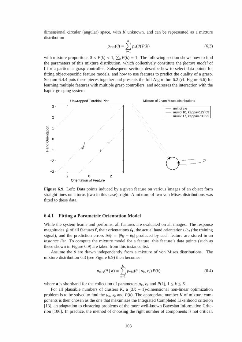
dimensional circular (angular) space, withK unknown, and can be represented as a mixturedistribution

pmix(θ) =K

∑

k=1

pk(θ) P(k) (6.3)

with mixture proportions 0< P(k) < 1,∑

k P(k) = 1. The following section shows how to findthe parameters of this mixture distribution, which collectively constitute thefeature modeloff for a particular grasp controller. Subsequent sections describe how to select data points forfitting object-specific feature models, and how to use features to predict the quality of a grasp.Section 6.4.4 puts these pieces together and presents the full Algorithm 6.2 (cf. Figure 6.6) forlearning multiple features with multiple grasp controllers, and addresses the interaction with thehaptic grasping system.

−2 0 2−3

−2

−1

0

1

2

3

Unwrapped Toroidal Plot

Orientation of Feature

Han

d O

rient

atio

n

Mixture of 2 von Mises distributions

unit circle mu=0.10, kappa=122.09mu=2.17, kappa=700.92

Figure 6.9. Left: Data points induced by a given feature on various images of an object formstraight lines on a torus (two in this case); right: A mixtureof two von Mises distributions wasfitted to these data.

6.4.1 Fitting a Parametric Orientation Model

While the system learns and performs, all features are evaluated on all images. The responsemagnitudesff of all featuresf , their orientationsθf , the actual hand orientationsθH (the trainingsignal), and the prediction errors∆θf = |θH − θh| produced by each feature are stored in aninstance list. To compute the mixture model for a feature, this feature’s data points (such asthose shown in Figure 6.9) are taken from this instance list.

Assume theθ are drawn independently from a mixture of von Mises distributions. Themixture distribution 6.3 (see Figure 6.9) then becomes

pmix(θ | a) =K

∑

k=1

pvM(θ | µk, κk) P(k) (6.4)

wherea is shorthand for the collection of parametersµk, κk andP(k), 1 ≤ k ≤ K.For all plausible numbers of clustersK, a (3K − 1)-dimensional non-linear optimization

problem is to be solved to find theµk, κk andP(k). The appropriate numberK of mixture com-ponents is then chosen as the one that maximizes the Integrated Completed Likelihood criterion[13], an adaptation to clustering problems of the more well-known Bayesian Information Crite-rion [106]. In practice, the method of choosing the right number of components is not critical,

103

because as better features are learned, the clusters of datapoints will become increasingly wellseparated.

For a particular value ofK, a maximum-a-posteriori (MAP) estimate of a mixture model isa parameterizationa that maximizes the posterior probability given by Bayes’ rule:

p(a | Θ) =L(Θ | a) p(a)

∑

m L(Θ | am) p(am)

whereL(Θ | a) is the likelihood of the observed dataΘ = {θ1, . . . , θN}. We now assume auniform prior probability density over all possible model parameterizationsam. In this case,the MAP estimate is identical to the maximum-likelihood estimate that maximizes the log-likelihood of the data:

logL(Θ | a) =N

∑

i=1

log pmix(θi | a) (6.5)

An elegant way to fit mixture models such as this is via the Expectation-Maximization (EM)algorithm. The EM algorithm is most practical if the model parametersµk, κk and P(k) canbe computed in closed form at the Expectation step. Unfortunately, this is not possible herebecause the Bessel functions cannot be inverted algebraically (see the Appendix). Facing thisadded difficulty, the mixture model (6.4) is more easily fitted directly, subject to the applicableconstraints on theκk andP(k), via gradient descent using the partial derivatives of theobjectivefunction (6.5):

∂

∂µklogL(Θ | a) =

N∑

i=1

P(k)pmix(θi | a)

∂

∂µkpvM(θi | µk, κk)

∂

∂κklogL(Θ | a) =

N∑

i=1

P(k)pmix(θi | a)

∂

∂κkpvM(θi | µk, κk)

where

∂

∂µpvM(θ | µ, κ) = κ sin(θ − µ) pvM(θ | µ, κ), (6.6)

∂

∂κpvM(θ | µ, κ) = − I−1(κ) + I1(κ) − 2I0(κ) cos(θ − µ)

2I0(κ)pvM(θ | µ, κ). (6.7)

TheK−1 partial derivatives with respect toP(k) must take into account the constraint∑K

k=1 P(k) =1:

∂

∂P(k)log L(Θ | a)

=∂

∂P(k)

N∑

i=1

log

K−1∑

k=1

pvM(θi | µk, κk) P(k) + pvM(θi | µK , κK)

1−K−1∑

k=1

P(k)

=

N∑

i=1

1pmix(θi | a)

(

pvM(θi | µk, κk) − pvM(θi | µK, κK))

, k = 1, . . . ,K − 1.

Each feature is annotated with its model parameters, which include theµk, κk, P(k), and thetotal numberNf of valid data points modeled by this mixture.

6.4.2 Selecting Object-Specific Data Points

If different types of objects are encountered, dedicated featuresmay have to be learned. Withouta supervisor providing object identities, the data collections (Figure 6.9) will be an indiscernible

104

mix of feature responses corresponding to various objects,and any reliable patterns will beobscured. The key to learning dedicated features is to ignore data points corresponding to weakfeature responses. This permits features to emerge that respond strongly only to specific, highlycharacteristic object parts, but that respond weakly in anyimage that does not contain such anobject. These weak responses will be ignored, and reliable models ofθ can be fitted to the strongresponses.

Deciding whether a given point is “strong” in this sense involves a threshold. Such thresh-olds αf , specific to each feature, can be determined optimally in theBayesian sense that thenumber of poor recommendations made by the resulting model is minimized.1 To do this for agiven featuref , the history of feature responsesff and the associated prediction errors∆θf areanalyzed in order to find a thresholdαf such that most predictions for cases withff > αf arecorrect. To formalize this intuitive notion, a global threshold t∆θ is introduced, meaning thata prediction with∆θf < t∆θ is correct, and false otherwise. The optimal thresholdαf is thendefined as a value that maximizes the Kolmogorov-Smirnoff distance KSDf between the twoconditional distributions offf under the two conditions that the associated predictions are cor-rect and false, respectively (Figure 6.10). The feature model of f is then fitted to all data pointsθ with ff > αf . The thresholdt∆θ is a global run-time parameter that can gradually be reducedover time to encourage the learning of improved features.

10

1

KSDf

cum

ula

tive

pro

bab

ility

false predictions:

αffeature responseff

∆θf ≥ t∆θcorrectpredictions:∆θf < t∆θ

Figure 6.10. Kolmogorov-Smirnoff distance KSDf between the conditional distributions offeature response magnitudes given correct and false predictions.

6.4.3 Predicting the Quality of a Grasp

The quality of a grasp is defined by the minimum friction coefficientµ0 required to execute thegrasp using a given finger configuration (cf. Section 6.3.1).In this model, the lower (closer tozero) a value ofµ0, the better the grasp. It is not possible to separate good from poor graspsbased on a generic threshold onµ0 alone because, for any given object, the best achievablegrasp depends on the object properties, the number of fingers, and – in general – on the end-to-end task. For example, the best achievable grasp of a triangular prism using two fingersis far worse than if three fingers are used. Under Coelho’s formulation, cubes are best graspedwith two fingers to take advantage of symmetric contact forces across parallel opposing surfaces(Figure 6.8).

It is possible to estimate the expected value ofµ0 associated with a given featuref . Forthis purpose, the actually experienced value ofµ0 is stored in the instance list along with each

1Bayesian optimality holds only under the assumption that the prior probabilities of the two conditions are equal.See Sections 4.3.2 and 4.4.1 for a discussion.

105

executed grasp. Theseµ0 values are regarded as samples of a continuous random variable M0

with probability density functionp(µ0) and expected value

E[M0] =∫ ∞

0µ0 p(µ0) dµ0.

Observe that each measured value ofµ0 is associated with the measured prediction error∆θf =

|θH − θh|, generated by the same grasp. Iff is indeed highly predictive of the grasp outcome,then there should be an approximate proportional relationship between theµ0 and the∆θf : Goodgrasps with smallµ0 should tend to exhibit a small angular error∆θf . Thus, the probabilitydensity functionp(µ0) should be well approximated by the distributionpvM(∆θf ) of the angularoffsets observed between the feature and hand orientations. Therefore, a sample estimate ofE[M0(f )] for featuref can be approximated as

E[M0(f )] =∑

i µ0,i pvM(∆θf ,i)∑

i pvM(∆θf ,i)(6.8)

where the corresponding pairs ofµ0,i and∆θf ,i are taken from the instance list, using only in-stances corresponding to occurrences off with ff ,i > αf .

6.4.4 Feature Learning Algorithm

Using the concepts introduced in the preceding sections, the procedure for fitting a feature modelis summarized in the following algorithm.

Algorithm 6.1 (Fitting a Feature Model) For a given featuref , the following steps are takento compute the associated orientation model, consisting oftheµk, κk, KSDf , andE[M0(f )]:

1. Using the current value oft∆θ, identify those occurrences off in the instance list thatcorrespond to correct and false predictions. Using the response magnitudesf of theseoccurrences, compute KSDf and the associated thresholdαf (Section 6.4.2).

2. Using theNf of these instances withf > αf , fit a parametric orientation model (Equation6.4), obtainingKf , and values forµk, κk, andP(k), k = 1, . . . ,Kf (Section 6.4.1).

3. Using this orientation model and the values ofµ0 and∆θf corresponding to the measure-ments off in the instance list, computeE[M0(f )] (Equation 6.8, Section 6.4.3).

The system operates by recommending hand orientations and observing the outcomes ofgrasping procedures. New features are added to the repertoire in parallel to the execution ofgrasping tasks, and are evaluated over the course of many future grasps. This is in contrast tothe distinction-learning application (Chapter 4), where the discriminative power of new featureswas immediately estimated using example images. Here, no example images are necessary. Thevisual system does not have any influence on the types or identities of the grasped objects. Twoseparate feature setsF2 andF3 and two separate instance lists are maintained for two- and three-fingered grasps. Out of these two sets, the feature with the lowest expected friction coefficientµ0 provides a recommendation of grasp parameters to the hapticsystem. The operation of thelearning system is detailed in the following algorithm.

Algorithm 6.2 (Feature Learning and Application of Feature Models) Initially, the setsF2

andF3 of features known to the system are empty.

1. A new grasp task is presented to the grasping system, and anoverhead image of the graspedobject is acquired.

2. The following steps are performed for each feature setFc:

106

(a) The responsesff of all featuresf ∈ Fc are measured in the current image.

(b) Identify the above-threshold feature with the highest predictive power:

f ∗c = argmaxf∈{f∈Fc| ff>αf }

KSDf

Now, choose the numberc of grasp contacts that will result in the better grasp:

c = argminc∈{2,3}

E[M0(f ∗c)]

3. From theK components in the angular mixture model associated withf ∗c, identify the mostconcentrated component distribution of angular errors:

k∗ = argmaxk∈

{

1≤k≤Kf∗c

∣

∣

∣

∣

Nf∗c P(k)≥3}

κk

To avoid singular modes, the maximum is only taken over thosecomponent distributionsthat model at least three data points.

4. Using the orientation off ∗c measured in the image and the angular offset associated withk∗, form a recommended hand orientation (cf. Equation 6.2):

θh = θf ∗c + µk∗

5. The robot performs ac-contact grasp with initial azimuthal angle ofθh. Upon convergenceof the haptic system, a new instance vector is added to the instance list, containing theresponse magnitudes, orientations, and prediction errors∆θf = |θH − θh| of all featuresf ∈ Fc, as well as the actual final hand orientationθH, and the achieved friction coefficientµ0.

6. If ∆θf ∗c < t∆θ, i.e. the recommended grasp parameters were accurate and required littleadjustment by the haptic system, then continue at Step 1.

7. Using Algorithm 6.1, the KSDf are recomputed for allf ∈ Fc, and all associated mix-ture models are re-estimated based on the cases recorded in the instance list of previousexperiences.

8. A new predictionθh is formed based on the new models, following the same procedure asabove, but leavingc fixed (Steps 2a, 2b, 3, 4).

9. If now |θH − θh| < t∆θ, continue at Step 1.

10. Add two new features toFc: One is created by sampling a random texel or a random pairof edgels from salient points in the current image (cf. Algorithm 4.10 (Feature Generation,page 43), Step 2). The other feature is generated by randomlyexpanding an existingfeature geometrically by adding a new point (cf. Algorithm 4.10, Step 3). Then, continueat Step 1.

Many of the features randomly sampled at Step 10 will performpoorly, e.g. because theyrespond to parts of the scene unrelated to the object to be grasped. Such features will developa poor KSD, as there is no systematic association between their response strengths and theirprediction accuracies. Due to their low KSD, such features will cease to be used at all (Step 2b).On the other hand, if a feature performs well, its KSD will be increased, and it will more likelybe employed. Moreover, since only features are consulted that are asserted to be present in theimage (i.e.,ff > αf ), features can be learned that selectively respond to different object shapesrequiring different offsetsθ. Unused features should be discarded periodically. The details

107

of when this is done are unimportant, but if all features are kept around, then those steps inAlgorithm 6.2 that involve iterating over all features willincur unnecessary computational cost.

This algorithm uses only a single feature to derive a hand orientation. Similarly to the pre-ceding two chapters, the reason for this choice is to reinforce the point that a highly uncommittedadaptive visual system can learn powerful features. The robustness of the recommended anglescan probably be increased by pooling the recommendations ofseveral features. At Step 2, thefeature of choice is determined according to its KSDf . Then, at Step 3, one of the modesk of thisfeature’s model is chosen to form the actual prediction. At first glance, it seems that this choiceof a model is unstable because the actual reliability of the individual modes of a given featuremodel may differ widely. However, this variation does not cause instability because the KSD isderived according to the actual behavior of the feature in practice, as recorded in the instancelist. Thus, a high KSD can only result if the practically usedmodesk perform consistently well.

In contrast to the feature learning algorithm for distinctive features (Algorithm 4.8 on page 41),Algorithm 6.2 does not evaluate features immediately, as this would require repeated grasps ofthe same object in lieu of the example images used by Algorithm 4.8. This algorithm insteadchooses to spread the evaluation of newly sampled features across multiple future grasps. Thisprevents the use of an explicit simple-to-complex search procedure such as Algorithm 4.10.However, the expansion of features at Step 10 above has the same effect, spread over multi-ple grasps. Boolean compound features are not used here because their orientations are lessmeaningful than those of geometric compounds.

Incidentally, this search for good predictive models constitutes an Expectation-Maximiza-tion (EM) algorithm. An EM algorithm alternates between estimating a set of unknown datavalues based on a current estimate of a model (Expectation step), and estimating the modelbased on the full data (Maximization step). Here, the parametric model to be optimized is thecollection of all feature-specific models that are used by the angular recommendation process.The unknown data values specify which recorded data points should participate in the feature-specific models. At the Expectation step, these hidden parameters are estimated by computingthe KSDf such that the probability of making the right choice for eachdata point is maximized,given the current model. At the Maximization step, the likelihood of the model given the par-ticipating data points is maximized by optimizing the modelparameters according to Equation6.5. As the system operates, these two steps alternate.

This instance of the EM algorithm is unusual in that the Expectation step does not utilizeall available current data. Instead, the instance list of past experiences is consulted for previ-ous prediction results, which were generated by models derived from all data availableat thattime. Taking the correct expectation using the most recent modelwould involve revisiting allpreviously-seen images at each Expectation step, which is clearly impractical. Nevertheless, theconvergence properties of the EM algorithm are unaffected. As data accumulate, the accuracy ofrecent expectations can only increase, and the influence of possibly inaccurate data from earlyhistory diminishes.

6.5 Experiments

The learning algorithm just presented is designed to operate on-line. However, a single graspperformed by the real robot using Coelho’s system (Section 6.3.1) takes on the order of tenminutes, while the learning algorithm requires hundreds ofgrasps to converge. Therefore, athorough on-line evaluation was impractical. Instead, experiments were conducted in simula-tion in a way that closely resembles the actual integrated grasping system. These experimentsutilized a detailed kinematic and dynamic simulator of the robotic hand/arm system, developedby Jefferson Coelho, that cycles through the following steps:

108

1. Generate a random polyhedral object geometry by drawing object parameters from para-metric probability distributions derived from actual experiments using the real robot. Ran-dom parameters include the dimensions and angles defining the object.

2. Perform a simulated grasp of this object. The haptic control system is the same as thatused for the real robot. The simulator interprets the motor commands and generates sen-sory feedback in the form of joint angles and (relatively noisy) force/torque readings ofthe fingertip sensors.

The three types of object geometries used included quadrangular (roughly square) and triangu-lar (roughly equilateral) prisms, and cylinders. Typical object geometries and converged graspconfigurations are illustrated in Figure 6.11. The ray originating from the object center indi-cates the wrist orientation in accordance with Figure 6.7. The categorization into “good” and“poor” grasps is for illustration only. As mentioned earlier, there is no way to grasp a trianglewell using two fingers, and all grasps of the cylinder were of consistently high quality. Visualinput for the visual learning system was generated by producing photo-realistically renderedand noise-degraded views on the basis of the object specifications generated at Step 1 above(Figure 6.12). All results reported below were computed in two-fold cross-validation. For sim-plicity and speed, no texels were used. However, other unpublished experiments indicate thatthe presence or absence of texels does not have a noticeable impact on this task.

Good Grasps Poor Grasps

Figure 6.11. Representative examples of synthesized objects and converged simulated graspconfigurations using Coelho’s haptically-guided graspingsystem.

Figure 6.12.Example views of objects used in the grasping simulations.

6.5.1 Training Visual Models

To generate training data, Coelho’s grasp simulator performed several hundred simulated graspson instances of the three object types, using two- and three-fingered grasp controllers, and

109

recorded the final grasp configurations on convergence, along with the grasp quality indexµ0.These data were used by Algorithm 6.2 to train visual featuremodels. Lacking the ability toperform an actual grasp at Step 5, the recommended grasps were simulated by comparing therecommended hand orientationθh with the previously executed hand orientationθH associatedwith the training image, modulo the known rotational symmetry properties of the object. Sincecylinders have infinite-fold rotational symmetry, any handorientation works equally well. Con-sequently, no features were ever learned for cylinders.

0 2 4 6 8 10 120

2

4

6

8Accuracy (clean, separated data)

Error [degrees]

Cou

nt

0 20 40 600

5

10

15

20Accuracy (noisy, unseparated data)

Error [degrees]C

ount

(a) (b)

Figure 6.13. Quantitative results of hand orientation prediction. The rightmost bin of the righthistogram includes all cases where the prediction error exceeded 60 degrees.

Figure 6.13 demonstrates that the system succeeds in learning features that are indicative ofhand orientations. The data in Figure 6.13a were produced byfeature models that were trainedusing 2-fold cross validation on the 20 best two-fingered grasps of cubes, and the 20 best three-fingered grasps of triangular prisms available in the simulated training set. As always in thischapter, the quality of a grasp was assessed in terms of the friction coefficient µ0. These datacan be expected to contain only little noise in the training signal, i.e., the actual hand orientationθH on grasp convergence. Performance on an independent test set is almost always excellent,with prediction error magnitudes on the order of the variation in the training signal.

The data in Figure 6.13b were produced by feature models thatwere trained on a represen-tative sample of 80 grasps, including 20 grasps each of cubesand triangular prisms using two-and three-fingered grasp controllers. On such noisy training data that contains hand orientationsthat produced a poor grasp, the system expends a lot of effort trying to learn these outliers. How-ever, performance degrades gracefully because features are selected by Kolmogorov-Smirnoffdistance, which prefers generic features that work well forthe majority of useful training exam-ples. On a noisy test set, most poor recommendations occur onoutliers. Notably, two-fingeredgrasps of the triangular object are inherently unstable andunpredictable. Here, prediction errorsproduced by the trained system depend on the error thresholdthat divides “good” from “poor”predictions during training. Choosing a low threshold generally produces more accurate predic-tions on a test set, as long as this threshold is larger than the variation contained in the majorityof the training data.

6.5.2 Using Visual Models to Cue Haptic Grasping

Several experiments were performed to evaluate the effect of visual priming on the haptic grasp-ing procedure. The two primary evaluation criteria were thenumber of haptic probes executedbefore the grasp controller converged, and the quality of the achieved grasp on convergence interms of the friction coefficient µ0. All experiments employ the native grasp controllers de-scribed in Section 6.3.1.

In the first experiment, a two-fingered native grasp controller was cued using features trainedon the best 20 two-fingered grasps of cubes available in the training set. An analogous experi-

110

0 5 10 15 200

100

200

300

400Native Haptic (Cubes/2)

Number of Probes

Cou

nt

0 5 10 15 200

50

100

150Visual+Haptic (Cubes/2)

Number of Probes

Cou

nt

0 0.5 10

500

1000Native Haptic (Cubes/2)

µ0

Cou

nt

0 0.5 10

100

200

300Visual+Haptic (Cubes/2)

µ0

Cou

nt

0 5 10 15 200

100

200

300Native Haptic (Triangles/3)

Number of Probes

Cou

nt

0 5 10 15 200

50

100Visual+Haptic (Triangles/3)

Number of Probes

Cou

nt

0 0.5 10

100

200

300Native Haptic (Triangles/3)

µ0

Cou

nt

0 0.5 10

50

100Visual+Haptic (Triangles/3)

µ0

Cou

nt

Figure 6.14. Results on two-fingered grasps of cubes (top half), and three-fingered grasps oftriangular prisms (bottom half). The left column shows purely haptic grasps; in the right column,grasps were cued using learned visual feature models. The rightmost bin in each histogramincludes all instances with a number of probes≥ 20, orµ0 ≥ 1, respectively.

111

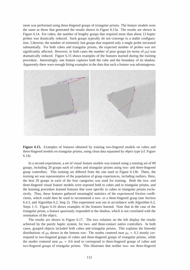
ment was performed using three-fingered grasps of triangular prisms. The feature models werethe same as those that generated the results shown in Figure 6.13a. The results are shown inFigure 6.14. For cubes, the number of lengthy grasps that required more than about 13 hapticprobes was drastically reduced. Such grasps typically do not converge to a stable configura-tion. Likewise, the number of extremely fast grasps that required only a single probe increasedsubstantially. For both cubes and triangular prisms, the expected number of probes was notsignificantly affected. However, in both cases the number of poor grasps (in terms ofµ0) wasdramatically reduced. Figure 6.15 shows examples of the features learned during the trainingprocedure. Interestingly, one feature captures both the cube and the boundary of its shadow.Apparently there were enough fitting examples in the data that such a feature was advantageous.

Figure 6.15. Examples of features obtained by training two-fingered models on cubes andthree-fingered models on triangular prisms, using clean data separated by object type (cf. Figure6.14).

In a second experiment, a set of visual feature models was trained using a training set of 80grasps, including 20 grasps each of cubes and triangular prisms using two- and three-fingeredgrasp controllers. This training set differed from the one used in Figure 6.13b: There, thetraining set was representative of the population of grasp experiences, including outliers. Here,the best 20 grasps in each of the four categories was used for training. Both the two- andthree-fingered visual feature models were exposed both to cubes and to triangular prisms, andthe learning procedure learned features that were specific to cubes or triangular prisms exclu-sively. Thus, these features gathered meaningful statistics of the experienced friction coeffi-cients, which could then be used to recommend a two- or a three-fingered grasp (see Section6.4.3, and Algorithm 6.2, Step 2). This experiment was run inaccordance with Algorithm 6.2,Steps 1–5. Figure 6.16 shows examples of the features learned. Note that in the case of thetriangular prism, a feature spuriously responded to the shadow, which is not correlated with theorientation of the object.

The results are shown in Figure 6.17. The two columns on the left display the resultsachieved by the purely haptic system, for two- and three-contact native controllers. In bothcases, grasped objects included both cubes and triangular prisms. This explains the bimodaldistributions ofµ0 shown in the bottom row: The modes centered nearµ0 = 0.2 mostly cor-respond to two-fingered grasps of cubes and three-fingered grasps of triangular prisms, whilethe modes centered nearµ0 = 0.6 tend to correspond to three-fingered grasps of cubes andtwo-fingered grasps of triangular prisms. This illustratesthat neither two- nor three-fingered

112

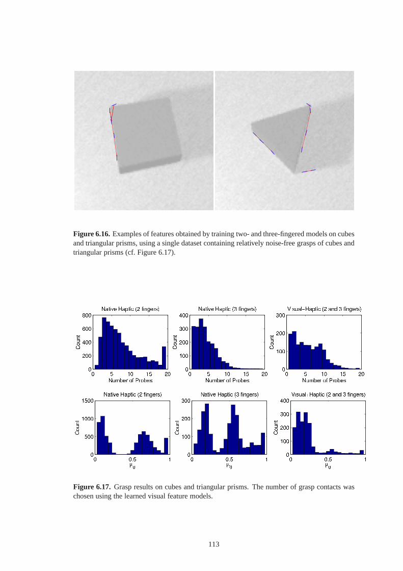
Figure 6.16.Examples of features obtained by training two- and three-fingered models on cubesand triangular prisms, using a single dataset containing relatively noise-free grasps of cubes andtriangular prisms (cf. Figure 6.17).

Figure 6.17. Grasp results on cubes and triangular prisms. The number of grasp contacts waschosen using the learned visual feature models.

113

native controllers alone are sufficient to execute high-quality grasps reliably for both cubes andtriangular prisms.

The rightmost column shows the results achieved if the learned visual models determinewhich native policy to use, and how to orient the hand at the outset of a grasp. Almost all graspsresult in a very goodµ0; the second mode has almost completely disappeared. Moreover, verylong trials (more than about 20 probes) are practically eliminated (cf. the two-fingered nativecontroller on the left). However, the expected number of probes increases slightly. The reasonsfor this undesired effect are unclear. One possible explanation is that the angular recommen-dations made by the learned feature models were relatively poor, and possibly skewed by asystematic bias, due to the presence of many unreliable grasps in the training set, predominantlytwo-fingered grasps of triangular prisms. Even if this is true, this slight drawback is more thanoutweighed by the enormous gain in the quality of the resulting grasps, as evidenced by the lowvalues ofµ0.

6.6 Discussion

This chapter described a system for learning to recommend hand orientations and finger con-figurations to a haptically-guided grasping system. Localized appearance-based features of thevisual scene are learned that correlate reliably with observed hand orientations. If the trainingdata are not overly noisy, specialized features emerge thatrespond to distinct object classes.These can then be used to recommend the number of grasp contacts to be used, based on theexpected quality of the grasp. In this way, visual guidance takes place without prior knowl-edge, explicit segmentation or geometric reconstruction of the scene. The interaction betweenhaptic and visual system is a plausible model of human grasping behavior. Learning is on-lineand incremental; there is no distinction between learning and execution phases. The resultsdemonstrate the feasibility of the concept.

The main limitation of the system, as used in the experimentsabove, is that its performancewas adversely affected by noise in the training data. It was unable to identifyand ignore noisytraining examples. However, it is important to note that this effect is inherent in the off-line na-ture of the training process. While the algorithm is designed to operate on-line, the experimentsabove were generated off-line using a fixed set of training data. In effect, the visual systemlearned solely by observing the haptic system in action. Without additional information, therewas no way for it to distinguish good from poor grasp outcomes. Off-line training severs animportant feedback loop between the visual and the haptic system. During on-line training, asdescribed in Algorithm 6.2, the haptic system always uses the cues given by the visual system.If these cues are accurate, then the quality of the resultinggrasps is of consistently high quality(Figures 6.14 and 6.17). In effect,once highly predictive features emerge, the resulting trainingdata will contain little noise!Due to the KSD feature selection metric, good features will beused more often than poor features. Thus, their increased use will change the distribution of thetraining data, with the effect that the noise is increasingly reduced. This is a strong reason toexpect that an on-line training procedure will bootstrap itself to yield reliable features by pro-ducing pure training data, which are in turn produced by reliable features. A merely observantlearner is permanently confronted with the same stationarydistribution of noisy training data,and wastes a lot of effort trying to learn the noise, contaminating its feature setwith spuriousfeatures. In contrast, an interactive learner can activelyeliminate the noise from the trainingdata! The experimental verification of this argument must beleft to future work.

The sensorimotor grasping system described in this chapterlearns about objects, and howthey are best grasped. This way of learning about activity afforded by the environment is remi-niscent of the Gibsonian ecological approach to perception[41, 39]. The notion ofaffordancesis a central concept in this theory. An affordance refers to the fit between an agent’s capa-bilities and the environmental properties that make possible given actions. According to the

114

Gibsons, an agent learns about affordances by interacting with the environment. It discoverseffects of actions and perceptual characteristics indicativeof affordances. The ecological ap-proach emphasizes that perception isdirect; behaviorally useful information is extracted moreor less directly from the egocentric sensory stream, without intermediate comprehensive rep-resentations such as geometric models. The Gibsonian theory is appealing to many roboticistsbecause of its direct link between perception and action. Unfortunately, the underlying com-putational mechanisms are largely unclear. This is addressed by the methods described in thischapter. The haptic sensorimotor system learns about the types of grasps afforded by differentobjects, that is, the fit between hand and object. At the same time, the visual system learns to as-sociate these affordances with visual appearance. Features of appearance are extracted directlyfrom the sensory stream, which is compatible with the Gibsonian notion of direct perception. Itwill be interesting to explore such activity-driven learning mechanisms in more elaborate taskscenarios.

115

CHAPTER 7

CONCLUSIONS

The first two chapters of this dissertation outlined a scenario in which autonomous robots re-fine their perceptual skills with growing experience, as demanded by their interaction with theenvironment. The following four technical chapters introduced a general framework for learn-ing useful visual features, and applied it to two very different task domains. This final chaptercollects the insights gained in the technical chapters, andreassembles them into parts of the bigpicture drawn at the outset. It discusses the contributionsof this dissertation, and highlightssome important directions for future research.

7.1 Summary of Contributions

The desire to construct autonomous robots that perform nontrivial tasks in the real world isone of the driving forces of research in artificial intelligence. It has long been argued thatthe world is too complex to allow the design of canned, robustaction policies. Therefore,learning capabilities are generally agreed to be a crucial ingredient of sophisticated autonomousrobots. However, the computer vision research community has not as widely embraced thisviewpoint. In Section 1.2 I argued that visual learning is indispensable for agents that need toextract task-relevant information from uncontrolled environments. This dynamic and purposiveparadigm of vision is commonly calledactive vision[4, 15]. The crucial role of visual learningin active vision has been pointed out in its early days [10, 9]. Since then however, relatively littleemphasis has been placed on the learning aspects of task-driven vision, although some progressis being made [76]. A central aim of this dissertation is the advancement of visual learning asan essential ingredient of task-driven vision systems. Thefollowing items summarize the keycontributions of this dissertation:

• The field of computer vision has a strong tradition of viewingvision problems in isolation.Under this paradigm, the goal of vision is to generate scene descriptions for use by higher-level reasoning processes. I argue that this approach is inappropriate in many visual tasksthat arise in the context of autonomous systems, and insteadadvocate adaptive visualsystems that learn to extract just the information needed for a task.

• I proposed an iterative, on-line paradigm for task-driven perceptual learning that cyclesthrough sensation, action, and evaluation steps (Figures 2.1 on page 8, 4.2 on page 35,and 6.6 on page 102). Learning takes place only when needed, and is highly focused onsolving problems encountered on line. This view of incremental visual learning departsfrom established traditions in computer vision.

• Extending Amit and Geman’s work on combinatorial features [8, 5] and combining it withhighly expressive and biologically plausible feature primitives, I introduced an infinitecombinatorial and parametric feature space that contains useful features for a variety oftasks. Powerful features are sought in a simple-to-complexfashion by random samplingdirectly in training images.

117

• I demonstrated that powerful features can be learned in a task-driven manner by a generalsystem that starts out with very little prior commitment to any particular task scenario.To reinforce this message, my algorithms are designed to learn only a small number offeatures that are highly distinctive individually.

• In the context of visual recognition, I generalized the conventional true/false dichotomyof classification by a multi-class framework that allows each class to be treated separately.This paradigm unifies the traditional paradigms of object recognition and detection. I alsomotivated an implementation on the basis of multiple Bayesian networks. This represen-tation abandons the closed-world assumption made by conventional recognition systems.

• The efficacy of these algorithms and representations was evaluatedon object discrimina-tion tasks that simulated an on-line learning scenario.

• Motivated by the phenomenon of human expertise in visual recognition, I proposed amethod for learning improved features by introducing explicit requirements of discrim-inative power. As a result, test-set performance significantly improves according to allperformance metrics.

• On the basis of the feature space, I developed a method for learning features to recommendconfiguration parameters for a haptically-guided graspingsystem that resembles the wayhumans use visual information to pre-shape their hands while reaching for an object. Themethod results in improved grasps, without any explicit extraction or representation ofobject geometry.

Two very different applications demonstrated the potential of the general approach. The ob-ject discrimination task is essentially aclassificationproblem, with the goal of finding featuresthat are highly predictive of particular classes. A strongly focused feature search procedure ex-plicitly applies simple-to-complex search heuristics. Candidate features are evaluated immedi-ately, which requires a cooperative environment that can provide example images. The graspingtask mainly constitutes aregressionproblem. Here, features are sought whose image-plane ori-entations robustly correlate with hand orientations. Feature evaluation is distributed over manysuccessive grasping trials, and does not require example images. The simple-to-complex featureconstruction strategy is more implicit in this algorithm.

All experiments were performed in simulation. On-line learning tasks in real environmentswill benefit from an efficient implementation, especially if it capitalizes on the high degree ofparallelism inherent in the feature search algorithms. Importantly, the algorithms presented herecan in principle be applied in on-line, interactive tasks. This constitutes an advancement inthe technology for building autonomous robots that performon-line perceptual learning. Themethodology begins with an uncommitted learning system that makes far weaker assumptionsabout the world and the task than most existing vision systems. In particular, no explicit as-sumptions are made regarding object segmentation, contourextraction, presence of clutter orocclusions, the number of target objects or classes presentin a scene, or the number of classesto be learned. Nevertheless, target concepts are learned with remarkable accuracy, as reportedin Chapters 5 and 6.

In addition to advancing technology, this dissertation also contributes to our understandingof human perceptual learning in that it provides a computational model of feature development.Sections 2.1 and 5.1 presented strong evidence that humans learn features not unlike those con-tained in the feature space introduced in Chapter 3. For the first time, a detailed computationalmodel of feature learning was presented that explains many of the phenomena observed by psy-chologists [109, 107, 120, 38, 41, 39]. Key principles of themodel are biologically plausible,including the primitive features and the principle of composition. It is not unlikely that hu-mans perform a simple-to-complex feature search, producing empirically useful features that

118

are discarded or refined as required by additional experience. Clearly, biological vision systemsemploy more sophisticated features not contained in the constrained space used here, as will bediscussed in the following section.

7.2 Future Directions

The algorithms developed in this dissertation are far more general than the restricted scenariosused in the experiments. Much more systematic experimentation is required to illuminate theirproperties. The recognition system needs to be evaluated under the presence of multiple targetobjects, occlusions, and non-target clutter objects. Individual target classes should include dif-ferent objects, including highly heterogeneous sets of objects that differ widely in appearance.Incremental introduction of target classes (in the sense ofSection 5.4.4) requires further study,e.g. by examining the effect of presentation order on the learning process. Most importantly,both the recognition and the grasping system need to be integrated in real-world interactivetasks, breaking away from closed training sets. It was pointed out that both the expert learningand the grasping applications are expected to undergo a noticeable performance boost if train-ing data are generated dynamically. Possible testbeds include humanoid or autonomous mobilerobots, smart rooms, etc.

This dissertation explored two different paradigms of the general feature learning method.One was concerned with supervised classification, the otherwith regression. A third practicalparadigm that should be explored involves an agent that learns multi-step reactive policies ina reinforcement learning framework. The agent takes policyactionsbased on the currentlyobservedstate. The only feedback available to the agent consists of a scalar reward that may bedelayed over several policy actions, or may be given only at sparse intervals. In this framework,the state can be represented in terms of learned features that capture task-relevant informationabout the environment. For example, the agent can begin withan impoverished perceptualstate space such that all world states are aliased. Then, thefeature learning subsystem seeksperceptual features that resolve hidden state, similar in spirit to McCallum’s U-Tree algorithm[67].

The following sections discuss important limitations and possible enhancements of the ideasand methods developed in this dissertation, and outline howthese can be addressed by futureresearch.

7.2.1 Primitive Features and their Composition

The two specific primitive feature types that form the basis of the feature space introduced inChapter 3 were chosen because they constitute a small set andexpress complementary aspectsof appearance. For general tasks, other types of primitive features should be introduced. Twoof the most important features missing in the current systemare color and statistical texturefeatures. Gaussian-derivative features of color-opponent image signals have been explored forappearance-based object recognition [43]. Statistical features analyze the local intensity distri-bution without regard to their spatial organization, and thus complement the highly structuredand oriented texels. For example, such features would probably prove valuable in the (gray-scale) Mel task.

An important characteristic of the feature space introduced in Chapter 3 is that it can beaugmented almost arbitrarily by adding other types of primitive features and rules of composi-tion. These additions are not limited to visual operators, but can include information from otherperceptual modalities, or generally, any type of assertionabout the world. Different modalitiescan even be combined within the same compound feature through appropriate compositionalrules. For example, combining visual and haptic information using this framework would openup new perspectives in cross-modally-guided grasping.

119

The temporal and three-dimensional nature of the world gives rise to more features, manyof which fit into this framework. For example, primitive or compound features can be computedon optical flow or disparity fields. These features are easilyaccessible to interactive agents, andare likely important in many everyday scenarios.

The current parametric representation of compound features is not very plausible biolog-ically. For representations compatible with current knowledge about the organization of thevisual brain, Riesenhuber and Poggio’s model [96] can serveas a starting point.

7.2.2 Higher-Level Features

In its present form, the feature space contains primitive and compound features. This spaceexcludes many types of features that are very informative tohumans, but are not easily express-ible within this framework. Examples include Gestalt features such as parallelism, symmetry(axial and radial), and continuity of contours. Another example is cardinality. To illustrate, abicycle wheel has many spokes, and a triangle has three corners. These abstract concepts are notdirectly expressible by the current feature set, but appearto be very powerful cues to humansfor scene interpretation. Some higher-level features may in principle be learnable by composingthem from lower-level features.

7.2.3 Efficient Feature Search

The current feature learning algorithm engages a blind and random generate-and-test search pro-cedure in static images. The only guidance available is given in the form of salient points, whichconstrain the search space to points that are deemed to be most important, independently of thetask. In reality, there are much more powerful ways to draw attention to important features. Forexample, I postulate that the ability to track feature points of a moving object can give pow-erful cues about what appearance-based features are stableacross a wide range of viewpoints.Also, such tracking allows the construction of (at least partially) view-invariant features of localthree-dimensional object structure.

There may also be other, more direct ways to extract distinctive features, in the spirit ofdiscriminative eigen-subspaces. I doubt that this is always possible, as even humans do not –at least not always – extract distinctive features directlyin this way. On sufficiently difficultdiscrimination tasks, we struggle to identify distinctivefeatures unless they are pointed out tous. There is strong psychological evidence suggesting thatthe subjective discriminability andorganization of objects is altered by experience [107].

However, there is certainly much room for improvement on thecurrent, blind generate-and-test method. One interesting possibility is to design ameta-learning process that noticespatterns in the ways distinctive features are found, and thus learns how to look for good featuresefficiently.

7.2.4 Redundancy

Both mammalian and state-of-the-art feature-based computer vision systems owe their perfor-mance largely to their use of a large number of features [71, 104, 96, 77, 78, 8, 6, 82, 66]. Theresulting redundancy or overcompleteness creates robustness to various kinds of image varia-tion and degradation. The present work on feature learning purposely did not use this type ofredundancy because without it, the distinctive power of individual features – and thus the suc-cess in learning – stand out much more. However, for practical applications such redundancy isrequired to increase robustness. Future work should investigate ways of learning large numbersof partially redundant features that are still powerful individually.

Recall from Chapter 5 that the trained recognition system rarely produces wrong results.Almost all incorrect recognitions are either ignorant or ambiguous, which are caused by a fail-

120

ure to find all relevant distinctive features in an image. This is an artifact of the extremely smallnumber of features learned by the system. The availability of redundant features would greatlyenhance the likelihood of finding distinctive features, which in turn would strongly reduce thenumber of ambiguous and ignorant recognitions. This makes me very confident that an exten-sion of the current learning system with many redundant (butpowerful) features would achieveresults competitive with the best of today’s, much more specialized recognition systems.

7.2.5 Integrating Visual Skills

Along with related work, this dissertation demonstrated some of the great potential of appearance-based vision. However, there are tasks that are not solved onthe basis of appearance alone.There is a role for other techniques such as shape-from-X, geometric model matching, or afunctional interpretation of items seen. Currently, such different paradigms are usually appliedin isolation. We do not know how to integrate them into a unified whole, as the human visualsystem appears to do. Ideally, an autonomous robot should have at its disposal a repertoire ofessential visual tools, and should learn how to use these jointly or individually.

7.3 Uncommitted Learning in Open Environments

The above discussion pointed out some features and rules forcomposition that should be addedto extend the range of concepts expressible by the learning system. However, there are twoimportant caveats: First, the combinatorics of the featuresearch grow badly with the numberof primitives and rules (see Algorithm 4.10 on page 43). The second caveat is an instance ofa critical problem shared by all inductive learning systems1: Even if unlimited computationalresources were available to cope with arbitrary numbers of primitives and rules, having too manyof these will necessarily hurt the learning process. The more degrees of freedom are availableto an inductive learning system, the more ways exist to find patterns in the data. If the numberof degrees of freedom is large in relation to the number of variables in the data, many spuriouspatterns will be found. There is no way to know which of these are valid in the sense that theywill generalize to unseen test instances. Therefore, all inductive learners are necessarily limitedin their expressive power. The guiding principles implementing this limitation are collectivelycalled theinductive biasof the learner. In practice, the designer of a learning procedure musttailor the inductive bias to the presumed structure of the task.

A novelty of this work is the introduction of an infinite feature space based on commonlyused visual feature primitives, expressive enough to learntraining sets of almost any classifi-cation task – if necessary, by memorizing the training images. Without any guiding principles,this learning system would be bias free, and therefore unable to generalize. The bias is given bya simple-to-complex feature sampling procedure that makesthe learner prefersimplefeatures.The underlying assumption is that simple features generally provide for the best generalization,or in other words, that the “real” structure underlying a task tends to be expressible by simplefeatures from the feature space (cf. Section 3.6, page 28).

This assumption is not always true, as exemplified by the Mel task in Chapters 4 and 5. Thefeatures found by the learner worked well on the training set, but generalized poorly neverthe-less. It appears that the features represented accidental structure in the training set, which doesnot generalize to test images. In some cases, spurious structure represented by a feature maybe supported by a large number of training images. In other cases, it may be supported by onlyvery few images, resulting in overfitted features. Data setsthat violate the structural assump-tions reflected in the inductive bias are especially prone tothis problem. This is apparently true

1Informally, aninductivelearning system learns a function from training examples, and then generalizes to unseentest instances on the basis of this function.

121

of the Mel task, where simple combinations of edgels and texels did not tend to capture the realstructure in the data.

How do humans solve the bias problem? Adult humans seem to be able to learn fromvery few examples, and are often able to pick out distinctivefeatures with apparent ease. Isuspect that the answer is related to our – learned – ability to control our learning bias. Guidedby a wealth of background knowledge and functional understanding of the world, we are ableto constrain our feature space adaptively and efficiently, so that relevant structure in the datais easily found. In other words, humans are not simple inductive learners, but our learning issupplemented by insights into functional and causal structure of the world. Likewise for artificialsystems, the bias problem implies that straightforward inductive mechanisms are insufficient tobuild effective uncommitted learners; they must be supplemented by other mechanisms [124].

Notably, it seems plausible that this knowledge is itself acquired by inductive mechanisms.One can envision a hierarchy of inductive learners. Many learners learn specialized tasks on thebasis of low-level features such as sensory signals. Their output signals constitute highly struc-tured input signals to other learners, enabling these to learn functions that would be impossibleto learn directly using the low-level features, because of their excessive degrees of freedom.These learning components can be trained in order, individually and largely independently, gen-erally from the bottom up. This order can be given by a teacherwho knows effective learningschedules. Where does the teacher come from? Imagine a worldpopulated by a large number ofsuch multilayer learning agents, all of which apply random learning schedules in an attempt todiscover useful structure in the world. Because of their large number, some of them will even-tually be successful. These can then become teachers of the others, sharing their empiricallysuccessful learning strategies.

This dissertation made progress toward building uncommitted perceptual systems that canlearn to become expert at specific tasks. The next quantum leap toward understanding humanlearning on the one hand, and toward constructing autonomous artificial learning systems foropen environments on the other hand, requires the defeat of the bias problem. This poses a greatchallenge to computer vision and machine learning research.

122

APPENDIX

EXPECTATION-MAXIMIZATION FOR VON MISES MIXTURES

The Expectation-Maximization (EM) algorithm [28] is an elegant class of methods for estimat-ing the parametersa of a probabilistic model where only some of the underlying variables areknown. The EM algorithm begins with any suitable initial estimate of the parametersa, andthen alternates the following two steps until convergence:

Expectation: Given the current estimate of the model parametersa and the observed data,compute the expected values of the unobserved portion of thedata.

Maximization: Given the observed data and the expected values of the unobserved data, com-pute a new set of model parametersa that maximizes some objective function.

If the objective function is continuous, this procedure will converge to a local maximum.A typical application of EM is the estimation of the parameters of a mixture model

pmix(θ | a) =K

∑

k=1

p(θ | ak) P(k) (A.1)

to fit an observed setΘ of data pointsθi , i = 1, . . . ,N. The mixing proportionsP(k) andthe componentski that generated each data pointθi are unknown. The objective is to find theparameter vectorak describing each component densityp(θ | ak).

The Expectation step computes the probabilitiesP(k | θi) that each data pointθi was gener-ated by componentk, given the current parameter estimatesak andP(k), using Bayes’ Rule:

P(k | θi) =p(θi | ak) P(k)

∑Kj=1 p(θi | a j) P( j)

=p(θi | ak) P(k)

pmix(θ | a)(A.2)

At the Maximization step, a new set of parametersak, k = 1, . . . ,K, is computed to maximizethe log-likelihood of the observed data:

logL(Θ | a) =N

∑

i=1

log pmix(θ | a) (A.3)

At the maximum, the partial derivatives with respect to all parameters vanish:

0 =∂

∂aklog L(Θ | a) =

N∑

i=1

P(k)pmix(θ | a)

∂

∂akp(θi | ak)

=

N∑

i=1

P(k | θi)p(θi | ak)

∂

∂akp(θi | ak) (A.4)

where the second line (A.4) follows from substituting Equation A.2. The Maximization is thencomputed by solving this system (A.4) for allak. Moreover, the estimates of the component

123

priors are updated by averaging the data-conditional component probabilities computed at theExpectation step:

P(k) =1N

N∑

i=1

P(k | θi) (A.5)

For the particular case of a mixture of von Mises distributions, Equation A.4 is instantiatedfor the parametersµ andκ for each mixture componentk. For µk, Equation A.4 becomes (cf.Equation 6.6, page 104)

∂

∂µklogL(Θ | a) = κ

N∑

i=1

P(k | θi) sin(θi − µk) = 0 (A.6)

µk = ± sin−1

N∑

i=1

P(k | θi) sinθi

√

√

√ N∑

i=1

N∑

j=1

P(k | θi) P(k | θ j) cos(θi − θ j)

(A.7)

Only one of the two solutions given by Equation A.7 is actually a root of Equation A.6. Whichone this is can be determined by backsubstitution into Equation A.6. The root ˆµk thus determinedeither minimizes or maximizes the log-likelihood (A.3), ascan be verified by consulting thesecond derivative:

∂2

∂2µklogL(Θ | a) = −κ

N∑

i=1

P(k | θi) cos(θi − µk) (A.8)

If the second derivative (A.8) at ˆµk is less than zero, thenµk = µk maximizes the log-likelihood(A.3); otherwise, ˆµk minimizes the log-likelihood, and its mirror image on the circle,µk = µk+π,is to be used instead.

In the case ofκ, the partial derivatives (cf. Equation 6.7)

∂

∂κklogL(Θ | a) = −

N∑

i=1

P(k | θi)I−1(κk) + I1(κk) − 2I0(κk) cos(θ − µk)

2I0(κk)= 0

cannot be solved forκk in closed form because the modified Bessel functions are not invertiblealgebraically. Theκk have to be approximated via numerical optimization, e.g. gradient de-scent. In other words, each iteration of the EM algorithm involvesk one-dimensional numericaloptimizations. In the face of this complexity, it seems simpler to perform a single (3K − 1)-dimensional numerical optimization to find the parametersµk, κk, andP(k) of the mixture model(A.1) directly, instead of using the iterative EM algorithm.

124

BIBLIOGRAPHY

[1] Acredolo, L. P. Behavioral approaches to spatial orientation in infancy. InThe Devel-opment and Neural Bases of Higher Cognitive Functions, A. Diamond, Ed., vol. 608.Annals of the New York Academy of Sciences, 1990, pp. 596–607.

[2] Acredolo, L. P., Adams, A., and Goodwyn, S. W. The role of self-produced movementand visual tracking in infant spatial orientation.Journal of Experimental Child Psychol-ogy 38(1984), 312–327.

[3] Allen, P. K. Surface descriptions from vision and touch.In Proceedings of the 1984Conference on Robotics(Atlanta, GA, Mar. 1984), IEEE, pp. 394–397.

[4] Aloimonos, Y., Weiss, I., and Bandopadhay, A. Active vision. International Journal ofComputer Vision 1(1988), 333–356.

[5] Amit, Y., and Geman, D. Shape quantization and recognition with randomized trees.Neural Computation 9(1997), 1545–1588.

[6] Amit, Y., and Geman, D. A computational model for visual selection.Neural Computa-tion 11, 7 (Oct. 1999), 1691–1715.

[7] Amit, Y., Geman, D., and Jedynak, B. Efficient focusing and face detection. InFaceRecognition: From Theory to Applications, H. Wechsler, P. Phillips, V. Bruce, F. F.Soulie, and T. Huang, Eds., NATO ASI Series F. Springer, Berlin, 1998.

[8] Amit, Y., Geman, D., and Wilder, K. Joint induction of shape features and tree classifiers.IEEE Transactions on Pattern Analysis and Machine Intelligence 19, 11 (1997), 1300–1305.

[9] Bajcsy, R., and Campos, M. Active and exploratory perception. Computer Vision, Graph-ics, and Image Processing: Image Understanding 56, 1 (July 1992), 31–40.

[10] Ballard, D. H. Animate vision.Artificial Intelligence 48(1991), 57–86.

[11] Ballard, D. H., Hayhoe, M. M., Pook, P. K., and Rao, R. P. N. Deictic codes for theembodiment of cognition.Behavioral and Brain Sciences 20, 4 (Dec. 1995), 723–767.

[12] Banks, M. S., Aslin, R. N., and Letson, R. D. Sensitive period for the development ofhuman binocular vision.Science 190(November 1975), 675–677.

[13] Biernacki, C., Celeux, G., and Govaert, G. Assessing a mixture model for clustering withthe integrated completed likelihood.IEEE Transactions on Pattern Analysis and MachineIntelligence 22, 7 (July 2000), 719–725.

[14] Black, M. J., and Jepson, A. D. EigenTracking: Robust matching and tracking of artic-ulated objects using a view-based representation. InEuropean Conference on ComputerVision (Cambridge, UK, 1996), pp. 329–342.

[15] Blake, A., and Yuille, A., Eds.Active Vision. MIT Press, Cambridge, Massachusetts,1992.

125

[16] Califano, A., and Mohan, R. Multidimensional indexingfor recognizing visual shapes.IEEE Transactions on Pattern Analysis and Machine Intelligence 16, 4 (April 1994),373–392.

[17] Canny, J. A computational approach to edge detection.IEEE Transactions on PatternAnalysis and Machine Intelligence 8, 6 (1986), 679–698.

[18] Cho, K., and Dunn, S. M. Learning shape classes.IEEE Transactions on Pattern Analysisand Machine Intelligence 16, 9 (1994), 882–888.

[19] Chomat, O., Colin de Verdiere, V., Hall, D., and Crowley, J. L. Local scale selectionfor Gaussian based description techniques. InEuropean Conference on Computer Vision(2000).

[20] Chomat, O., and Crowley, J. Probabilistic recognitionof activity using local appear-ance. InProceedings of the IEEE Computer Society Conference on Computer Vision andPattern Recognition (CVPR ’99)(Ft. Collins, CO, June 1999), vol. 2, IEEE ComputerSociety, pp. 104–109.

[21] Coelho, Jr., J. A., and Grupen, R. A. A control basis for learning multifingered grasps.Journal of Robotic Systems 14, 7 (1997), 545–557.

[22] Coelho, Jr., J. A., and Grupen, R. A. Dynamic control models as state abstractions. InNIPS’98 Workshop on Abstraction and Hierarchy in Reinforcement Learning(Brecken-ridge, CO, 1998).

[23] Coelho, Jr., J. A., and Grupen, R. A. Learning in non-stationary conditions: A con-trol theoretic approach. InProceedings of the Seventeenth International Conference onMachine Learning(2000), Morgan Kaufmann.

[24] Coelho, Jr., J. A., Piater, J. H., and Grupen, R. A. Developing haptic and visual per-ceptual categories for reaching and grasping with a humanoid robot. InFirst IEEE-RASInternational Conference on Humanoid Robots(2000).

[25] Cohen, P. R., Atkin, M. S., Oates, T., and Beal, C. R. Neo:Learning conceptual knowl-edge by sensorimotor interaction with an environment. InProceedings of the First Inter-national Conference on Autonomous Agents(1997), pp. 170–177.

[26] Colin de Verdiere, V., and Crowley, J. L. Visual recognition using local appearance. InFifth European Conference on Computer Vision(June 1998), vol. 1 ofLecture Notes inComputer Science, Springer, pp. 640–654.

[27] de Jong, E. D., and Steels, L. Generation and selection of sensory channels. InEvolution-ary Image Analysis, Signal Processing and Telecommunications First European Work-shops, EvoIASP’99 and EuroEcTel’99 Joint Proceedings(Berlin, May 1999), LNCS,Springer-Verlag, pp. 90–100.

[28] Dempster, A. P., Laird, N. M., and Rubin, D. B. Maximum likelihood from incompletedata via the EM algorithm.Journal of the Royal Statistical Society (Series B) 39, 1(1977), 1–38.

[29] Draper, B. A., Bins, J., and Baek, K. ADORE: Adaptive object recognition.Videre 1, 4(2000), 86–99.

[30] Fisher, N. I.Statistical Analysis of Circular Data. Cambridge University Press, 1993.

[31] Fisher, R. A.Contributions to Mathematical Statistics. John Wiley, New York, 1950.

126

[32] Fisher, R. B., and MacKirdy, A. Integrating iconic and structured matching. InEuropeanConference on Computer Vision(1998).

[33] Fleuret, F., and Geman, D. Graded learning for object detection. Tech. rep., Departmentof Mathematics and Statistics, University of Massachusetts, Amherst, Feb. 1999.

[34] Florack, L. M. J. The Syntactic Structure of Scalar Images. PhD thesis, University ofUtrecht, 1993.

[35] Freeman, W. T., and Adelson, E. H. The design and use of steerable filters.IEEE Trans-actions on Pattern Analysis and Machine Intelligence 13, 9 (1991), 891–906.

[36] Friedman, J. H., and Tukey, J. W. A projection pursuit algorithm for exploratory dataanalysis.IEEE Transactions on Computers 23(1974), 881–890.

[37] Fukunaga, K., and Koontz, W. L. G. Applications of the Karhunen-Loeve expansion tofeature selection and ordering.IEEE Transactions on Computers C-19(1970), 917–923.

[38] Gauthier, I., and Tarr, M. J. Becoming a “Greeble” expert: Exploring mechanisms forface recognition.Vision Research 37, 12 (1997), 1673–1682.

[39] Gibson, E. J., and Pick, A.An Ecological Approach to Perceptual Learning and Devel-opment. Oxford University Press, in press.

[40] Gibson, E. J., and Spelke, E. S. The development of perception. In Handbook of ChildPsychology Vol. III: Cognitive Development, J. H. Flavell and E. M. Markman, Eds.,4th ed. Wiley, 1983, ch. 1, pp. 2–76.

[41] Gibson, J. J.The Ecological Approach to Visual Perception. Houghton Mifflin, Boston,1979.

[42] Grimson, W. E. L., and Lozano-Perez, T. Model-based recognition and localization fromtactile data.Journal of Robotics Research 3, 3 (1986), 3–35.

[43] Hall, D., Colin de Verdiere, V., and Crowley, J. L. Object recognition using colouredreceptive fields. InEuropean Conference on Computer Vision(2000).

[44] Held, R. Binocular vision – behavioral and neuronal development. InNeonate Cognition:Beyond the Blooming Buzzing Confusion, J. Mehler and R. Fox, Eds. Lawrence ErlbaumAssociates, 1985, pp. 37–44. Reprinted in [53], pp. 152–158.

[45] Hubel, D. H., and Wiesel, T. N. Receptive fields, binocular interaction and functionalarchitecture in the cat’s visual cortex.Journal of Physiology (London) 160(1962), 106–154.

[46] Huttenlocher, D. P., and Ullman, S. Recognizing solid objects by alignment with animage.International Journal of Computer Vision 5, 2 (1990), 195–212.

[47] Intrator, N. Feature extraction using an unsupervisednetwork. Neural Computation 4(1992), 98–107.

[48] Intrator, N., and Gold, J. I. Three-dimensional objectrecognition using an unsupervisedBCM network: The usefulness of distinguishing features.Neural Computation 5(1993),61–74.

[49] Jagersand, M., and Nelson, R. Visual space task specification, planning and control. InProc. IEEE Symposium on Computer Vision(1995), pp. 521–526.

127

[50] Jedynak, B., and Fleuret, F. Reconnaissance d’objets 3D a l’aide d’arbres de classifica-tion. In Image’Com ’96(Bordeaux, France, 20–22 May 1996).

[51] Jensen, F. V.An introduction to Bayesian networks. Springer, New York, May 1996.

[52] John, G. H., Kohavi, R., and Pfleger, K. Irrelevant features and the subset selction prob-lem. InProceedings of the Eleventh International Conference on Machine Learning(SanFrancisco, 1994), W. W. Cohen and H. Hirsh, Eds., Morgan Kaufmann.

[53] Johnson, M. H., Ed.Brain Development and Cognition. Bracewell, New York, 1993.

[54] Kandel, E. R., Schwartz, J. H., and Jessell, T. M., Eds.Essentials of Neural Science andBehavior. Appleton & Lange, Stamford, Connecticut, 1995.

[55] Knoll, T. F., and Jain, R. C. Recognizing partially visible objects using feature indexedhypotheses.IEEE Journal of Robotics and Automation RA-2, 1 (March 1986), 3–13.

[56] Koenderink, J. J. The structure of images.Biological Cybernetics 50(1984), 363–370.

[57] Koenderink, J. J., and van Doorn, A. J. Representation of local geometry in the visualsystem.Biological Cybernetics 55(1987), 367–375.

[58] Kruger, N., and Ludtke, N. ORASSYLL: Object recognition with autonomously learnedand sparse symbolic representations based on local line detectors. InBritish MachineVision Conference(1998).

[59] Kruskal, J. B. Linear transformation of multivariate data to reveal clustering. InMultidi-mensional Scaling: Theory and Application in the Behavioural Sciences, R. N. Shephard,A. K. Romney, and S. K. Nerlove, Eds. Seminar Press, New York,1972, pp. 179–191.

[60] Lauritzen, S. L. Propagation of probabilities, means,and variances in mixed graphicalmodels. Journal of the American Statistical Association (Theory and Methods) 87, 420(1992), 1098–1108.

[61] Leonardis, A., and Bischof, H. Robust recognition using eigenimages.Computer Visionand Image Understanding 78, 1 (Apr. 2000), 99–118.

[62] Lindeberg, T. Scale-Space Theory in Computer Vision. Kluwer Academic Publishers,Dordrecht, Netherlands, 1994.

[63] Lindeberg, T. Edge detection and ridge detection with automatic scale selection.Inter-national Journal of Computer Vision 30, 2 (1998), 117–154.

[64] Lindeberg, T. Feature detection with automatic scale selection. International Journal ofComputer Vision 30, 2 (1998), 77–116.

[65] Logothetis, N. K., and Pauls, J. Psychophysical and physiological evidence for viewer-centered object representation in the primate.Cerebral Cortex 3(1995), 270–288.

[66] Lowe, D. G. Towards a computational model for object recognition in IT cortex. InProceedings of the IEEE International Workshop on Biologically Motivated ComputerVision (May 2000), S.-W. Lee, H. H. Bulthoff, and T. Poggio, Eds., vol. 1811 ofLNCS,Springer-Verlag, pp. 20–31.

[67] McCallum, A. K. Reinforcement Learning with Selective Perception and Hidden State.PhD thesis, Department of Computer Science, University of Rochester, Rochester, NY,1995. Revised 1996.

128

[68] McCallum, R. A. Overcoming incomplete perception withutile distinction memory. InProceedings of the Tenth International Conference on Machine Learning(1993), MorganKaufmann.

[69] McCallum, R. A. Utile suffix memory for reinforcement learning with hidden state.Tech. Rep. 549, Dept. of Computer Science, University of Rochester, Rochester, NY,Dec. 1994.

[70] McCarty, M. E., Clifton, R. K., Ashmead, D. H., Lee, P., and Goubet, N. How infantsuse vision for grasping objects.Child Development(in press).

[71] Mel, B. W. SEEMORE: Combining color, shape, and texturehistogramming in aneurally-inspired approach to visual object recognition.Neural Computation 9(1997),777–804.

[72] Moghaddam, B., and Pentland, A. Probabilistic visual learning for object representation.IEEE Transactions on Pattern Analysis and Machine Intelligence 19, 7 (July 1997), 696–710.

[73] Murase, H., and Nayar, S. K. Visual learning and recognition of 3-D objects from ap-pearance.International Journal of Computer Vision 14(1995), 5–24.

[74] Nayar, S. K., Murase, H., and Nene, S. A. Learning, positioning, and tracking visualappearance. InProceedings of the International Conference on Robotics and Automation(San Diego, CA, May 1994), IEEE.

[75] Nayar, S. K., Nene, S. A., and Murase, H. Subspace methods for robot vision. IEEETransactions on Robotics and Automation 12, 5 (Oct. 1996), 750–758.

[76] Nayar, S. K., and Poggio, T., Eds.Early Visual Learning. Oxford University Press, Feb.1996.

[77] Nelson, R. C., and Selinger, A. A cubist approach to object recognition. InProceedingsof the International Conference on Computer Vision(1998).

[78] Nelson, R. C., and Selinger, A. Large-scale tests of a keyed, appearance-based 3-D objectrecognition system.Vision Research 38, 15–16 (1998).

[79] Nene, S. A., Nayar, S. K., and Murase, H. Columbia objectimage library (COIL-20).Tech. Rep. CUCS-005-96, Columbia University, New York, Feb. 1996.

[80] Olshausen, B. A., and Field, D. J. Emergence of simple-cell receptive-field properties bylearning a sparse code for natural images.Nature 381(1996), 607–609.

[81] Papageorgiou, C. P., Oren, M., and Poggio, T. A general framework for object detection.In Proceedings of the International Conference on Computer Vision(Jan. 1998).

[82] Papageorgiou, C. P., and Poggio, T. A pattern classification approach to dynamical objectrecognition. InProceedings of the International Conference on Computer Vision(Corfu,Greece, Sept. 1999).

[83] Pearl, J.Probabilistic Reasoning in Intelligent Systems: Networksof Plausible Inference.Morgan Kaufmann, San Francisco, 1988.

[84] Piater, J. H., and Grupen, R. A. A framework for learningvisual discrimination. InProceedings of the Twelfth International FLAIRS Conference (1999), Florida ArtificialIntelligence Research Society, AAAI Press, pp. 84–88.

129

[85] Piater, J. H., and Grupen, R. A. Learning visual recognition with Bayesian networks.Computer Science Technical Report 99-43, University of Massachusetts, Amherst, MA,Mar. 1999.

[86] Piater, J. H., and Grupen, R. A. Toward learning visual discrimination strategies. InProceedings of the IEEE Computer Society Conference on Computer Vision and PatternRecognition(June 1999), vol. 1, IEEE Computer Society, pp. 410–415.

[87] Piater, J. H., and Grupen, R. A. Constructive feature learning and the development ofvisual expertise. InProceedings of the Seventeenth International Conference on MachineLearning(2000), Morgan Kaufmann, pp. 751–758.

[88] Piater, J. H., and Grupen, R. A. Distinctive features should be learned. InProceedingsof the IEEE International Workshop on Biologically Motivated Computer Vision(May2000), S.-W. Lee, H. H. Bulthoff, and T. Poggio, Eds., vol. 1811 ofLNCS, Springer-Ver-lag, pp. 52–61.

[89] Piater, J. H., and Grupen, R. A. Feature learning for recognition with Bayesian networks.In Proceedings of the International Conference on Pattern Recognition (Sept. 2000).

[90] Rao, R. P. N., and Ballard, D. H. An active vision architecture based on iconic represen-tations.Artificial Intelligence 78(1995), 461–505.

[91] Rao, R. P. N., and Ballard, D. H. Dynamic model of visual recognition predicts neuralresponse properties in the visual cortex.Neural Computation 9, 4 (May 1997), 721–763.

[92] Ravela, S., and Manmatha, R. Retrieving images by appearance. InProceedings of theInternational Conference on Computer Vision(1998), pp. 608–613.

[93] Ravela, S., and Manmatha, R. Gaussian filtered representations of images. InThe Ency-clopedia on Electrical& Electronics Engineering, J. G. Webster, Ed. John Wiley & Sons,1999, pp. 289–307.

[94] Ravela, S., Manmatha, R., and Riseman, E. M. Image retrieval using scale space match-ing. In Fourth European Conference on Computer Vision(Cambridge, U.K., April 1996),Springer, pp. 273–282.

[95] Rider, E. A., and Rieser, J. J. Pointing at objects in other rooms: Young children’ssensitivity to perspective after walking with and without vision. Child Development 59(1988), 480–494.

[96] Riesenhuber, M., and Poggio, T. Hierarchical models ofobject recognition in cortex.Nature Neuroscience 2(1999), 1019–1025.

[97] Rieser, J. J., Garing, A. E., and Young, M. F. Imagery, action, and young children’s spatialorientation: It’s not being there that counts, it’s what onehas in mind.Child Development65 (1994), 1262–1278.

[98] Rimey, R. D., and Brown, C. M. Task-oriented vision withmultiple Bayes nets. InActiveVision, A. Blake and A. Yuille, Eds. MIT Press, Cambridge, Massachusetts, 1992, ch. 14,pp. 217–236.

[99] Ripley, B. D. Pattern Recognition and Neural Networks. Cambridge University Press,1996.

130

[100] Riseman, E. M., Hanson, A. R., Beveridge, J. R., Kumar,R., and Sawhney, H. Landmark-based navigation and the acquisition of environmental models. In Visual Navigation:From Biological Systems to Unmanned Ground Vehicles, Y. Aloimonos, Ed. LawrenceErlbaum Associates, 1997, ch. 11, pp. 317–374.

[101] Ruff, H. A. Infant recognition of the invariant form of objects.Child Development 49(1978), 293–306.

[102] Russell, S., and Norvig, P.Artificial Intelligence: A Modern Approach. Prentice-Hall,Upper Saddle River, NJ, 1995.

[103] Salapatek, P., and Banks, M. S. Infant sensory assessment: Vision. InCommunicativeand Cognitive Abilities – Early Behavioral Assessment, F. D. Minifie and L. L. Lloyd,Eds. University Park Press, Baltimore, 1978.

[104] Schiele, B., and Crowley, J. L. Object recognition using multidimensional receptive fieldhistograms. InFourth European Conference on Computer Vision(Cambridge, UK, Apr.1996).

[105] Schnackertz, T. J., and Grupen, R. A. A control basis for visual servoing tasks. InProceedings of the International Conference on Robotics and Automation(1995), IEEE.

[106] Schwarz, G. Estimating the dimensions of a model.Annals of Statistics 6(1978), 461–464.

[107] Schyns, P. G., Goldstone, R. L., and Thibaut, J.-P. Thedevelopment of features in objectconcepts.Behavioral and Brain Sciences 21, 1 (1998), 1–54.

[108] Schyns, P. G., and Murphy, G. L. The ontogeny of part representation in object concepts.In The Psychology of Learning and Motivation, Medin, Ed., vol. 31. Academic Press,San Diego, CA, 1994, pp. 305–354.

[109] Schyns, P. G., and Rodet, L. Categorization creates functional features.Journal of Ex-perimental Psychology: Learning, Memory, and Cognition 23, 3 (1997), 681–696.

[110] Segen, J. Learning graph models of shape. InProceedings of the 5th InternationalConference on Machine Learning(Ann Arbor, June 12–14 1988), J. Laird, Ed., MorganKaufmann, pp. 29–35.

[111] Shams, S. Multiple elastic modules for visual patternrecognition.Neural Networks 8, 9(1995), 1439–1456.

[112] Shannon, C. E., and Weaver, W.The mathematical theory of communication. Universityof Illinois Press, Urbana, 1949.

[113] Solso, R. L., and McCarthy, J. E. Prototype formation of faces: A case of pseudo-memory.British Journal of Psychology 72(1981), 499–503.

[114] Steels, L. Constructing and sharing perceptual distinctions. InProceedings of the Euro-pean Conference on Machine Learning(Berlin, 1997), M. van Someren and G. Widmer,Eds., Springer-Verlag.

[115] Sutton, R. S., and Barto, A. G.Reinforcement Learning: An Introduction. MIT Press,Cambridge, Massachusetts, 1998.

[116] Swain, M. J., and Ballard, D. H. Color indexing.International Journal of ComputerVision 7, 1 (1991), 11–32.

131

[117] Swets, D. L., and Weng, J. Using discriminant eigenfeatures for image retrieval.IEEETransactions on Pattern Analysis and Machine Intelligence18, 8 (Aug. 1996), 831–836.

[118] Talukder, A., and Casasent, D. Classification and poseestimation of objects using nonlin-ear features. InApplications and Science of Computational Intelligence(1998), vol. 3390,SPIE.

[119] Talukder, A., and Casasent, D. A general methodology for simultaneous representationand discrimination of multiple object classes.Optical Engineering(Mar. 1998). Specialissue on Advances in Recognition Techniques.

[120] Tanaka, J. W., and Taylor, M. Object categories and expertise: Is the basic level in theeye of the beholder?Cognitive Psychology 23(1991), 457–482.

[121] Tarr, M. J. Visual pattern recognition. InEncyclopedia of Psychology, A. Kazdin, Ed.American Psychological Association, Washington, DC, in press.

[122] Tarr, M. J., and Bulthoff, H. H. Is human object recognition better described by geon-structural-descriptions or by multiple-views?Journal of Experimental Psychology: Hu-man Perception and Performance 21, 6 (1995), 1494–1505.

[123] Thibaut, J.-P. The development of features in children and adults: The case of visualstimuli. In Proc. 17th Annual Meeting of the Cognitive Science Society(1995), LawrenceErlbaum, pp. 194–199.

[124] Thrun, S., and Mitchell, T. M. Lifelong robot learning. Robotics and Autonomous Systems15 (1995), 25–46.

[125] Turk, M., and Pentland, A. Eigenfaces for recognition. Journal of Cognitive Neuroscience3, 1 (1991), 71–86.

[126] Utgoff, P. E., and Clouse, J. A. A Kolmogorov-Smirnoff metric for decision tree induc-tion. Computer Science Technical Report 96-3, University of Massachusetts, Amherst,1996.

[127] van Vliet, L. J., Young, I. T., and Verbeek, P. W. Recursive Gaussian derivative filters. InProc. 14th International Conference on Pattern Recognition (ICPR’98)(Brisbane, Aus-tralia, Aug. 1998), vol. 1, IEEE Computer Society Press, pp.509–514.

[128] Viola, P. A. Complex feature recognition: A Bayesian approach for learning to recognizeobjects. AI Memo 1591, Massachusetts Institute of Technology, November 1996.

[129] Wallis, G., and Bulthoff, H. Learning to recognize objects.Trends in Cognitive Science3, 1 (1999), 22–31.

[130] Weng, J., and Chen, S. Incremental learning for vision-based navigation. InProceedingsof the International Conference on Pattern Recognition(Vienna, Austria, 1996), pp. 45–49.

[131] Weng, J., and Chen, S. Vision-guided navigation usingSHOSLIF. Neural Networks 11(1998), 1511–1529.

[132] Young, R. A. The Gaussian derivative model for spatialvision: I. Retinal mechanisms.Spatial Vision 2, 4 (1987), 273–293.

[133] Zerroug, M., and Medioni, G. The challenge of generic object recognition. InObjectRepresentation in Computer Vision: Proc. NSF-ARPA Workshop (1994), pp. 217–232.

132

VISUAL FEATURE LEARNING - Universität Innsbruck

Documents

Transcript of VISUAL FEATURE LEARNING - Universität Innsbruck