Technikerstraße 13 - 6020 Innsbruck - Austria

Tel.: +43 512 507 53803 Fax: +43 512 507 53898

https://applied-math.uibk.ac.at

AppliedMathematics

Preprint-Series: Department of Mathematics - Applied Mathematics

The Averaged Kaczmarz Iteration for Solving Inverse Problems

Housen Li, Markus Haltmeier

Nr. 4114. September 2017

The Averaged Kaczmarz Iteration for Solving Inverse Problems

Housen Li

National University of Defense Technology137 Yanwachi street, 410073 Changsha, China

Email: housen.li@outlook.com

Markus Haltmeier

Department of Mathematics, University of InnsbruckTechnikestraße 13, A-6020 Innsbruck, Austria

Email: markus.haltmeier@uibk.ac.at

September 13, 2017

Abstract

We introduce a new iterative regularization method for solving inverse problems thatcan be written as systems of linear or non-linear equations in Hilbert spaces. The proposedaveraged Kaczmarz (AVEK) method can be seen as a hybrid method between the Landweberand the Kaczmarz method. As the Kaczmarz method, the proposed method only requiresevaluation of one direct and one adjoint sub-problem per iterative update. On the other,similar to the Landweber iteration, it uses an average over previous auxiliary iterates whichincreases stability. We present a convergence analysis of the AVEK iteration. Further,numerical studies are presented for a tomographic image reconstruction problem, namely thelimited data problem in photoacoustic tomography. Thereby, the AVEK is compared withother standard iterative regularization methods including the Landweber and the Kaczmarziteration.

Keywords: Inverse problems, system of ill-posed equations, regularization method, Kacz-marz iteration, ill-posed equation, convergence analysis, tomography, circular Radon trans-form.

AMS Subject Classification: 65J20; 65J22; 45F05.

1 Introduction

In this paper, we study the stable solution of linear or non-linear systems of operator equationsof the form

Fi(x) = yi for i = 1, . . . , n . (1.1)

Here Fi : D(Fi) ⊆ X → Yi are possibly nonlinear operators between Hilbert spaces X and Yi

with domains of definition D(Fi). We are in particular interested in the case that we only

1

have approximate data yδi ∈ Yi available, which satisfy an estimate of the form ‖yδ

i − yi‖ ≤ δifor some noise levels δi > 0. Moreover, we focus on the ill-posed (or ill-conditioned) case,where exact solution methods for (1.1) are sensitive to perturbations. Many inverse problems inbiomedical imaging, geophysics or engineering sciences can be written in such a form (see, forexample, [14, 29, 36].) For its stable solution one has to use regularization methods, which useapproximate but stable solution concepts.

There are at least two basic classes of solution approaches for inverse problems of theform (1.1), namely (generalized) Tikhonov regularization on the one and iterative regulariza-tion on the other hand. Both approaches are based on rewriting (1.1) as a single equationF(x) = y with forward operator F = (Fi)

ni=1 and exact data y = (yi)

ni=1. In Tikhonov

regularization, one defines approximate solutions as minimizers of the Tikhonov functional1n

∑ni=1 ‖Fi(x) − yδ

i ‖2 + λ‖x − x0‖2, which is the weighted combination of the residual term∑ni=1 ‖Fi(x) − yδ

i‖2 that enforces all equations to be approximately satisfied, and the regular-ization term ‖x−x0‖2 that stabilizes the inversion process. In iterative regularization methods,stabilization is achieved via early stopping of specially designed iterative schemes. For this classof methods, one develops special iterative optimization techniques designed for minimizing theun-regularized residual term

∑ni=1 ‖Fi(x) − yδ

i ‖2. The iteration index in this case plays therole of the regularization parameter which has to be carefully chosen depending on availableinformation about the noise and the unknowns to be recovered.

In this paper we consider the class of iterative regularization methods. We introduce a newmember of this class, named the averaged Kaczmarz (AVEK) iteration. The method combinesadvantages of two main iterative regularization techniques, namely the Landweber and theKaczmarz iteration.

1.1 Iterative regularization methods

The most basic iterative method for solving inverse problems is the Landweber iteration [14, 19,21, 25], which reads

∀k ∈ N : xδk+1 := xδ

k −skn

n∑

i=1

F′i(x

δk)∗

(Fi(x

δk) − yδ

i

). (1.2)

Here F′i(x)∗ is the Hilbert space adjoint of the derivative of Fi, sk is the step size and xδ

1 theinitial guess. The Landweber iteration renders a regularization method when stopped accordingto Morozov’s discrepancy principle, which stops the iteration at the smallest index k⋆ suchthat

∑ni=1 ‖Fi(x

δk⋆

) − yδi‖2 ≤ n(τδ)2 for some constant τ > 1. A convergence analysis of the

non-linear Landweber iteration has first been derived in [19]. Among others, similar resultshave subsequently been established for the steepest-descent method [30], the preconditionedLandweber iteration [12], or Newton-type methods [6, 35].

Each iterative update in (1.2) can be numerically quite expensive, since it requires solvingforward and adjoint problems for all of the n equations in (1.1). In situations where n is large andevaluating the forward and adjoint problems is costly, methods like the Landweber-Kaczmarziteration (see [13, 17, 18, 22, 23])

∀k ∈ N : xδk+1 := xδ

k − skαkF′[k](x

δk)∗

(F[k](x

δk) − yδ

[k]

), (1.3)

where [k] := (k−1 mod n)+1, are often much faster. The acceleration comes from the fact thatthe update in (1.3) only requires the solution of one forward and one adjoint problem instead

2

of several of them, but nevertheless often yields a comparable decrease per iteration of thereconstruction error. The additional parameters αk ∈ {0, 1} are introduced to effect that in thenoisy data case some of the iterative updates are skipped which renders the (1.3) a regularizationmethod. Such a skipping strategy has been introduced in [18] for the Landweber-Kaczmarziteration and later, among others, combined with steepest descent and Levenberg-Marquardttype iterations [3, 11]. These Kaczmarz type methods often perform well in practice, but lack ofconvergence in the absence of a common solution, even in the well-posed case. This can easilybe seen in the case of two linear equations in R without a common solution [27, Section 2], seealso [10, 38]. The AVEK method that we introduce in this paper overcomes this issue but isstill computationally efficient.

1.2 The averaged Kaczmarz iteration

The AVEK iteration is defined by

xδk+1 :=

1

n

k∑

ℓ=k−n+1

ξδℓ (1.4)

ξδℓ := xδℓ − sℓαℓF

′[ℓ](x

δℓ)

∗(F[ℓ](x

δℓ) − yδ

[ℓ]

)(1.5)

αℓ :=

{1 if ‖F[ℓ](x

δℓ) − yδ

[ℓ]‖ ≥ τ[ℓ]δ[ℓ]

0 otherwise. (1.6)

Instead of discarding the previous computations, in the AVEK iteration one remembers the lastKaczmarz type auxiliary iterates ξδℓ and the update xδ

k+1 is defined as the average over them.

The parameters αℓ effect that no update for ξδℓ is performed if ‖F[ℓ](xδℓ) − yδ

[ℓ]‖ is sufficientlysmall; τi ≥ 0 are control parameters. As the Kaczmarz iteration, the AVEK iteration onlyrequires evaluating a single gradient F′

i(x)∗(Fi(x) − yδi ) per iterative update which usually

is the numerically most expensive part for evaluating (1.4)-(1.6). On the other hand, as theLandweber iteration (1.2), each update in the AVEK uses information of all equations whichenhances stability. Further, note that the AVEK update can alternatively be written as xδ

k+1 =

xδk + (ξδk − ξδk−n)/n which can numerically be more efficient than evaluating (1.4).

In this paper we establish a convergence analysis of (1.4)-(1.6) for exact and noisy data(see Section 2). These results are most closely related to the convergence analysis of otheriterative regularization methods such as the Landweber and steepest decent methods [19, 30]and extensions to Kaczmarz type iterations [11, 18, 26]. However, the AVEK iteration is newand we are not aware of a convergence analysis for any similar iterative regularization method.We point out, that the AVEK shares some similarities with the incremental gradient methodof [7] and the averaged stochastic gradient method of [37] (both studied in finite dimensions).However, the iterations of [7, 37] are notably different from the AVEK method as they use anaverage of gradients instead of an average of auxiliary iterates (cf. Section 4).

1.3 Outline

The rest of this paper is organized as follows. In Section 2 we present the convergence analysisof the AVEK method under typical assumptions for iterative regularization methods. As mainresults we show weak convergence of AVEK in the case of exact data (see Theorem 2.6) and

3

converge as the noise level tends to zero (see Theorem 2.9). The proof of an important auxiliaryresult (Lemma 2.5) required for the convergence analysis is presented in Appendix A. In Sec-tion 3, we apply AVEK method to the limited view problem for the circular Radon transformand present a numerical comparison with the Landweber and the Kaczmarz method. The paperconcludes with a summary presented in Section 4 and a discussion of open issues and possibleextensions of AVEK.

2 Convergence analysis

In this section we establish the convergence analysis of the AVEK method. For that purpose wefirst fix the main assumptions in Subsection 2.1 and derive the basic quasi-monotonicity propertyof AVEK in Subsection 2.2. The actual convergence analysis is presented in Subsections 2.3and 2.4.

2.1 Preliminaries

Throughout this paper Fi : D(Fi) ⊆ X → Yi are continuously Frechet differentiable maps fori ∈ {1, . . . , n}. We consider the system (1.1), which can be written as a single equation F(x) = ywith forward operator F = (Fi)

ni=1 and exact data y = (yi)

ni=1 in Y :=

∏ni=1 Yi. Here y ∈ Y are

the exact data and yδ = (yδi )

ni=1 ∈ Y denote noisy data satisfying ‖yi − yδ

i ‖ ≤ δi with δi ≥ 0.For the convergence analysis of the AVEK method established below we assume that the

following additional assumptions are satisfied.

Assumption 2.1 (Main conditions for the convergence analysis).

(A1) There are x0 ∈ X, ρ > 0 such that Bρ(x0) := {x | ‖x− x0‖ ≤ ρ} ⊆ ⋂i∈{1,...,n}D(Fi).

(A2) For every i ∈ {1, . . . , n}, it holds sup{‖F′i(x)‖ | x ∈ Bρ(x0)} < ∞.

(A3) For every i ∈ {1, . . . , n}, there exists a constant ηi ∈ [0, 1/2) such that

∀x1,x2 ∈ Bρ(x0) : ‖Fi(x1) −Fi(x2) − F′i(x1)(x1 − x2)‖

≤ ηi‖Fi(x1) − Fi(x2)‖ . (2.1)

Equation (2.1) is often referred to as local tangential cone condition.

(A4) For the exact data y ∈ Y, there exists a solution of (1.1) in Bρ/3(x0).

From Assumption 2.1 it follows that (1.1) has at least one x0-minimum norm solution denotedx+ ∈ X. Such a minimal norm solution satisfies

‖x+ − x0‖ = inf{‖x− x0‖ | x ∈ Bρ(x0) and F(x) = y} .

The AVEK iteration is defined by (1.4)-(1.6). There we always choose the initialisation suchthat xδ

1, . . . ,xδn ∈ Bρ/3(x0) and assume that τi > 2(1 + ηi)/(1 − 2ηi).

4

2.2 Quasi-monotonicity

Opposed to the Landweber and the Kaczmarz method, for the AVEK method the reconstructionerror ‖xδ

k − x∗‖, where x∗ is a solution of (1.1), is not strictly decreasing. However, we canshow the following quasi-monotonicity property which plays a central role in our convergenceanalysis.

Proposition 2.2 (Quasi-monotonicity). Let x∗ ∈ Bρ(x0) be any solution of (1.1). Supposethat xδ

k is defined by (1.4)-(1.6), and that Assumption 2.1 holds true. Additionally, suppose thatthe step sizes sk are chosen in such a way that

sk‖F′i(x)‖2 ≤ 1 for every i, k and x ∈ Bρ(x0) . (2.2)

Then for every k ≥ n it holds that xδk ∈ Bρ(x0) and

‖xδk+1 − x∗‖2 ≤ 1

n

k∑

ℓ=k−n+1

‖xδℓ − x∗‖2

− 1

n

k∑

ℓ=k−n+1

sℓαℓ‖F[ℓ](xδℓ) − yδ

[ℓ]‖(

(1 − 2η[ℓ])‖F[ℓ](xδℓ) − yδ

[ℓ]‖ − 2(1 + η[ℓ])δ[ℓ]

). (2.3)

Proof. Assume for the moment that (2.1) and (2.2) are satisfied on the whole space X insteadonly on Bρ(x0). Then, for each ℓ ∈ N, we have

‖ξδℓ − x∗‖2 − ‖xδℓ − x∗‖2

= ‖ξδℓ − xδℓ‖2 + 2〈ξδℓ − xδ

ℓ ,xδℓ − x∗〉

≤ s2ℓα2ℓ‖F′

[ℓ](xδℓ)‖2‖F[ℓ](x

δℓ) − yδ

[ℓ]‖2 − 2sℓαℓ〈F′[ℓ](x

δℓ)

∗(F[ℓ](xδℓ) − yδ

[ℓ]),xδℓ − x∗〉

≤ sℓαℓ‖F[ℓ](xδℓ) − yδ

[ℓ]‖2 − 2sℓαℓ〈F[ℓ](xδℓ) − yδ

[ℓ],F′[ℓ](x

δℓ)(x

δℓ − x∗)〉

= sℓαℓ‖F[ℓ](xδℓ) − yδ

[ℓ]‖2 − 2sℓαℓ〈F[ℓ](xδℓ) − yδ

[ℓ],F[ℓ](xδℓ) − yδ

[ℓ]〉− 2sℓαℓ〈F[ℓ](x

δℓ) − yδ

[ℓ],F[ℓ](x∗) − F[ℓ](x

δℓ) + F′

[ℓ](xδℓ)(x

δℓ − x∗)〉

− 2sℓαℓ〈F[ℓ](xδℓ) − yδ

[ℓ],yδ[ℓ] − F[ℓ](x

∗)〉≤ −sℓαℓ‖F[ℓ](x

δℓ) − yδ

[ℓ]‖2 + 2η[ℓ]sℓαℓ‖F[ℓ](xδℓ) − yδ

[ℓ]‖‖F[ℓ](xδℓ) − F[ℓ](x

∗)‖+ 2sℓαℓδ[ℓ]‖F[ℓ](x

δℓ) − yδ

[ℓ]‖

≤ −sℓαℓ‖F[ℓ](xδℓ) − yδ

[ℓ]‖(

(1 − 2η[ℓ])‖F[ℓ](xδℓ) − yδ

[ℓ]‖ − 2(1 + η[ℓ])δ[ℓ]

).

From Jensen’s inequality it follows that

‖xδk+1 − x∗‖2 =

∥∥∥ 1

n

k∑

ℓ=k−n+1

(ξδℓ − x∗)∥∥∥2≤ 1

n

k∑

ℓ=k−n+1

‖ξδℓ − x∗‖2 ≤ 1

n

k∑

ℓ=k−n+1

‖xδℓ − x∗‖2

− 1

n

k∑

ℓ=k−n+1

sℓαℓ‖F[ℓ](xδℓ) − yδ

[ℓ]‖(

(1 − 2η[ℓ])‖F[ℓ](xδℓ) − yδ

[ℓ]‖ − 2(1 + η[ℓ])δ[ℓ]

).

5

Recall that there exists a solution ξ∗ of (1.1) in Bρ/3(x0) (which can be different from x∗).

Applying the above inequality to ξ∗ we obtain ‖xδk+1 − ξ∗‖2 ≤ 1

n

∑kℓ=k−n+1 ‖xδ

ℓ − ξ∗‖2. The

assumption ∀ℓ ≤ k : ‖xδℓ − ξ∗‖ ≤ 2ρ/3 therefore implies ‖xδ

k+1 − ξ∗‖ ≤ 2ρ/3. An inductive

argument shows that ‖xδk − ξ∗‖ ≤ 2ρ/3 indeed holds for all k ∈ N. Consequently, ‖xδ

k − x0‖ ≤‖xδ

k − ξ∗‖ + ‖ξ∗ − x0‖ ≤ ρ and therefore xδk ∈ Bρ(x0). Thus, for (2.3) to hold, it is in fact

sufficient that (2.1) and (2.2) are satisfied on Bρ(x0) ⊆ X.

The quasi-monotonicity property (2.3) implies that the squared error ‖xδk+1−x∗‖2 is smaller

than the average over n-previous squared errors. This is a basic ingredient for our convergenceanalysis. However, the absence of strict monotonicity makes the analysis more involved thanthe one of the Landweber and Kaczmarz iterations.

2.3 Exact data case

In this subsection we consider the case of exact data where δi = 0 for every i ∈ {1, . . . , n}. Inthis case, we have αℓ = 1 and we write the AVEK iteration in the form

∀k ≥ n : xk+1 =1

n

k∑

ℓ=k−n+1

(xℓ − sℓF

′[ℓ](xℓ)

∗(F[ℓ](xℓ) − y[ℓ])). (2.4)

We will prove weak convergence of (2.4) to a solution of (1.1). To that end we start with thefollowing technical lemma.

Lemma 2.3. Assume that (pk)k∈N is a sequence of non-negative numbers satisfying pk+1 ≤1n

∑kℓ=k−n+1 pℓ for all k ≥ n. Then (pk)k∈N is convergent.

Proof. Define qk := max {pℓ | ℓ ∈ {k − n + 1, . . . , k}}. Then qk is a non-increasing sequence andlimk→∞ qk = c for some c ≥ 0. Further, lim supk→∞ pk = c. Anticipating a contradiction,we assume that there exists some ǫ > 0 such that lim infk→∞ pk = c − 3ǫ. Then there are asubsequence (k(i) ∈ N)i∈N and a positive integer i0 such that pk(i) ≤ c− 2ǫ for all k(i) ≥ k(i0).Noting that lim supk→∞ pk = c, we can assume i0 being sufficiently large such that pk ≤ c+ ǫ/nfor all k ≥ k(i0). For ℓ = 1, . . . , n− 1 and k(i) ≥ k(i0), we have

pk(i)+ℓ ≤1

n

k(i)+ℓ∑

j=k(i)+ℓ−n+1

pj ≤n− 1

n

(c +

ǫ

n

)+

c− 2ǫ

n≤ c− ǫ

n.

Because pk ≤ max {pj | j ∈ {k(i0), . . . , k(i0) + n− 1}} ≤ c − ǫ/n for k ≥ k(i0), this contradictslim supk→∞ pk = c. We therefore conclude limk→∞ pk = c.

Some implications of the quasi-monotonicity of the AVEK iteration (see Proposition 2.2) arecollected next.

Lemma 2.4. Let Assumption 2.1 be satisfied and let x∗ ∈ Bρ(x0) be a solution of (1.1). Define(xk)k∈N by (2.4), where the step sizes sk satisfy (2.2). Then the following hold true:

(a) ‖xk − x∗‖ is convergent as k → ∞.

(b) If inf{sk | k ∈ N} > 0, then∑

k∈N ‖F[k](xk) − y[k]‖2 < ∞.

6

Proof. Proposition 2.2 for the case δi = 0 yields

‖xk+1 − x∗‖2 ≤ 1

n

k∑

ℓ=k−n+1

‖xℓ − x∗‖2 − 1

n

k∑

ℓ=k−n+1

(1 − 2η[ℓ])sℓ‖F[ℓ](xℓ) − y[ℓ]‖2 . (2.5)

This, together with Lemma 2.3, implies that ‖xk − x∗‖ is convergent as k → ∞. Summing (2.5)from k = n to k = m + n gives

n∑

i=1

i ‖xi+m+1 − x∗‖2 −n∑

i=1

i ‖xi − x∗‖2

≤ −m+n∑

k=n

k∑

ℓ=k−n+1

(1 − 2η[ℓ])sℓ‖F[ℓ](xℓ) − y[ℓ]‖2. (2.6)

Therefore, we have∑m+n

k=1 ‖F[k](xk) − y[k]‖2 ≤ 1M

∑ni=1 i‖xi − x∗‖2 < ∞ for all m ∈ N, with

constant M := (1 − 2 maxi=1,...,n ηi) infk∈N sk. The assertion follows by letting m → ∞.

For the Landweber and Kaczmarz iterations strict monotonicity of ‖xk − x∗‖ holds. Fromthis one can show that ‖xk+1−xk‖ converges to zero. The following Lemma 2.5 states that thesame result holds true for the AVEK iteration. However, its proof is much more involved andtherefore presented in the appendix.

Lemma 2.5. Under the assumptions of Lemma 2.4, we have limk→∞ ‖xk+1 − xk‖ = 0.

Proof. See Appendix A.

Now we are ready to show the weak convergence of the AVEK iteration (xk)k∈N. Thepresented proof uses ideas taken from [26].

Theorem 2.6 (Convergence for exact data). Let Assumption 2.1 hold and define (xk)k∈N by(2.4), with step sizes sk satisfying (2.2) and inf {sk | k ∈ N} > 0. Then the following hold:

(a) We have xk ⇀ x∗ as k → ∞, where x∗ ∈ Bρ(x0) is a solution of (1.1).

(b) If the initialisation is chosen as x1 = · · · = xn = x0, and

∀x ∈ Bρ(x0) : N(F′(x+)

)⊆ N

(F′(x)

)(2.7)

where x+ is an x0-minimal norm solution of (1.1), then xk ⇀ x+ as k → ∞.

Proof. (a): From Proposition 2.2 it follows that xk ∈ Bρ(x0) and therefore (xk)k∈N has at leastone weak accumulation point x∗. Suppose x is any weak accumulation point of (xk)k∈N andassume xk(j) ⇀ x as j → ∞. For every i = 1, . . . , n define ki(j) in such a way that [ki(j)] = iand k(j) ≤ ki(j) ≤ k(j) + n− 1. Then

∀i ∈ {1, . . . , n} : ‖xk(j) − xki(j)‖ ≤k(j)+n−2∑

ℓ=k(j)

‖xℓ+1 − xℓ‖ → 0 as j → ∞ .

By Lemma 2.4 we have ‖Fi(xki(j))−yi‖ → 0 as j → ∞, and therefore limj→∞ ‖Fi(xk(j))−yi‖ =0 for all i ∈ {1, . . . , n}. Together with [26, Proposition 2.2] this implies that x is a solution

7

of (1.1). Now assume that x is another weak accumulation point with x 6= x and that xm(j) ⇀ xas j → ∞. Then x and x are both solutions to (1.1). By Lemma 2.4 and [34, Lemma 1], weobtain

limk→∞

‖xk − x‖ = lim infj→∞

‖xk(j) − x‖ < lim infj→∞

‖xk(j) − x‖ = limk→∞

‖xk − x‖

and likewise limk→∞ ‖xk − x‖ < limk→∞ ‖xk − x‖. This leads to a contradiction and thereforethe weak accumulation point of (xk)k∈N is unique which implies xk ⇀ x∗.

(b): An inductive argument, together with the definition of xk shows

xk =

n∑

i=1

wi,kxi −k−1∑

l=1

cℓ,ksℓF′[ℓ](xℓ)

∗(F[ℓ](xℓ) − y[ℓ]

)

= x0 −k−1∑

l=1

cℓ,ksℓF′[ℓ](xℓ)

∗(F[ℓ](xℓ) − y[ℓ]

)

for some 0 < wi,k < 1 with∑n

i=1wi,k = 1 and 0 < cℓ,k < 1. Note that

∀x ∈ Bρ(x0) : R(F′i(x)∗

)⊆ N

(F′i(x)

)⊥ ⊆ N(F′(x)

)⊥ ⊆ N(F′(x+)

)⊥.

Thus xk ∈ x0 + N (F′(x+))⊥ and, by continuity of F′(x+), we have x∗ ∈ x0 + N (F′(x+))⊥.Together with [19, Proposition 2.1] we conclude x∗ = x+.

2.4 Noisy data case

Now we consider the noisy data case, where δi > 0 for i ∈ {1, . . . , n}. The AVEK iteration isthen defined by (1.4)–(1.6) and stopped at the index

k∗(δ) := min{ℓn ∈ N | xδ

ℓn = · · · = xδℓn+n−1

}. (2.8)

The following Lemma shows that the stopping index is well defined.

Lemma 2.7. The stopping index k∗(δ) defined in (2.8) is finite, and the corresponding residualssatisfy ‖Fi(x

δk∗(δ)) − yi‖ < τiδi for all i ∈ {1, . . . , n}.

Proof. Similar to (2.6), from Proposition 2.2 we obtain

m+n∑

k=n

k∑

ℓ=k−n+1

αℓsℓ‖F[ℓ](xδℓ) − yδ

[ℓ]‖(

(1 − 2η[ℓ])‖F[ℓ](xδℓ) − yδ

[ℓ]‖ − 2(1 + η[ℓ])δ[ℓ]

)

≤n∑

i=1

i‖xδi − x∗‖2.

Note that either ‖F[ℓ](xδℓ) − yδ

[ℓ]‖ ≥ τ[ℓ]δ[ℓ] or it holds αℓ = 0. If k∗(δ) is infinite, there are

infinitely many ℓ such that ‖F[ℓ](xδℓ)−yδ

[ℓ]‖ ≥ τ[ℓ]δ[ℓ]. This implies that the left hand side of the

above displayed equation tends to infinity as m → ∞, which gives a contradiction. Thus k∗(δ)is finite. Again by Proposition 2.2, we obtain ‖Fi(x

δk∗(δ)) − yi‖ < τiδi, for i = 1, . . . , n.

8

We next show the continuity of xδk at δ = 0. For that purpose denote

∆k(δ,y,yδ) :=

k∑

ℓ=k−n+1

αℓF′[ℓ](x

δℓ)

∗(F[ℓ](x

δℓ) − yδ

[ℓ]

)−

k∑

ℓ=k−n+1

F′[ℓ](xℓ)

∗(F[ℓ](xℓ) − y[ℓ]

).

Lemma 2.8. For all k ∈ N, we have

� limδ→0 sup{‖∆k(δ,y,yδ)‖ | ∀i = 1, . . . , n : ‖yδ

i − yi‖ ≤ δi}

= 0;

� limδ→0 xδk = xk.

Proof. We prove the assertions by induction. The case k ≤ n is shown similar to the generalcase and therefore omitted. Assume that k ≥ n + 1 and that the assertions hold for all m < k.It follows immediately that xδ

k → xk as δ → 0. Note that

∥∥∥∆k(δ,y,yδ)∥∥∥ ≤

k∑

ℓ=k−n+1

∥∥∥αℓF′[ℓ](x

δℓ)

∗(F[ℓ](x

δℓ) − yδ

[ℓ]

)− F′

[ℓ](xℓ)∗(F[ℓ](xℓ) − y[ℓ]

)∥∥∥ .

For each ℓ ∈ {k − n + 1, . . . , k}, we consider two cases. In the case αℓ = 1, the continuity of Fand F′ implies ‖F′

[ℓ](xδℓ)

∗(F[ℓ](xδℓ) − yδ

[ℓ]) −F′[ℓ](xℓ)

∗(F[ℓ](xℓ) − y[ℓ])‖ → 0 as δ → 0. In the case

αℓ = 0, we have ‖F[ℓ](xδℓ) − yδ

[ℓ]‖ < τ[ℓ]δ[ℓ] and therefore, as δ → 0,

‖F′[ℓ](xℓ)

∗(F[ℓ](xℓ) − y[ℓ])‖≤‖F′

[ℓ](xℓ)‖‖F[ℓ](xℓ) − y[ℓ]‖

≤‖F′[ℓ](xℓ)‖

(‖F[ℓ](xℓ) − F[ℓ](x

δℓ)‖ + ‖F[ℓ](x

δℓ) − yδ

[ℓ]‖ + ‖yδ[ℓ] − y[ℓ]‖

)

≤‖F′[ℓ](xℓ)‖

(‖F[ℓ](xℓ) − F[ℓ](x

δℓ)‖ + (1 + τ[ℓ])δ[ℓ]

)→ 0 .

Combining these two cases, we obtain ‖∆k(δ,y,yδ)‖ → 0 as δ → 0.

Theorem 2.9 (Convergence for noisy data). Let δ(j) := (δ1(j), . . . , δn(j)) be a sequence in(0,∞)n with limj→∞ maxi=1,...,n δi(j) = 0, and let y(j) = (y1(j), . . . ,yn(j)) be a sequence of

noisy data with ‖yi(j) − yi‖ ≤ δi(j). Define xδ(j)k by (1.4)-(1.6) with y(j) and δ(j) in place of

yδ and δ, and define k∗(δ(j)) by (2.8). Then the following assertions hold true:

(a) The sequence xδ(j)k∗(δ(j)) has at least one weak accumulation point and every such weak

accumulation point is a solution of (1.1).

(b) If, in the case of exact data, xk converges strongly to x∗, then limj→∞ xδ(j)k∗(δ(j)) = x∗.

(c) If the initializations are chosen as xδ(j)1 = · · · = x

δ(j)n = x0, and (2.7) is satisfied, then

each (strong or weak) limit x∗ is an x0-minimal norm solution of (1.1).

Proof. (a): By Proposition 2.2 the sequence x(j) := xδ(j)k∗(δ(j)) remains in Bρ(x0) and therefore

has at least one weak accumulation point. Let x∗ be a weak accumulation point of (x(j))j∈Nand (x(j(ℓ)))ℓ∈N a subsequence with x(j(ℓ)) ⇀ x∗ as ℓ → ∞. By Lemma 2.7 and the triangle

9

Γ

∂D(R) \ Γ

D(R)

fz

Figure 2.1: Recovering a function from the circular Radon transform. The functionf (representing some physical quantity of interest) is supported inside the disc D(R). Detectorsare placed at various locations on the observable part of the boundary Γ ⊆ ∂D(R) and recordaverages of f over circles with varying radii. No detectors can be placed at the un-observablepart ∂D(R) \ Γ of the boundary.

inequality, for every i ∈ {1, . . . , n} we have ‖Fi(x(j(ℓ))) − Fi(x∗)‖ ≤ 2δi(j(ℓ)) → 0 as ℓ → ∞.

Using [26, Proposition 2.2] we conclude that x∗ is a solution of (1.1).(b): We consider two cases. In the first case we assume that (k∗(δ(j)))j∈N is bounded. It is

sufficient to show that for each accumulation point k∗ of (k∗(δ(j)))j∈N, which is clearly finite,

it holds that limj→∞ xδ(j)k∗ = x∗. Without loss of generality, we can assume that k∗(δ(j)) = k∗

for all sufficiently large j. By Lemma 2.7, we have ‖Fi(xδ(j)k∗ ) − y

δ(j)i ‖ ≤ τiδi(j) and, by taking

the limit j → ∞, that Fi(xk∗) = yi. Thus, it holds that xk∗ = x∗ and therefore xδ(j)k∗ → x∗ as

j → ∞.In the second case, we assume lim supj→∞ k∗(δ(j)) = ∞. Without loss of generality, we can

assume that k∗(δ(j)) is monotonically increasing. For any ε > 0, there exists some m ∈ N with‖xm−i+1 − x∗‖ ≤ ε/2 for i = 1, . . . , n. An inductive argument, together with Proposition 2.2shows ‖xδ

k+m−x∗‖ ≤ ∑ni=1wi,k‖xδ

m−i+1−x∗‖ for certain weighs 0 < wi,k < 1 with∑n

i=1 wi,k =1. Then for sufficiently large j it holds that

‖xδ(j)k∗(δ(j)) − x∗‖ ≤ max

i=1,...,n‖xδ(j)

m−i+1 − x∗‖

≤ maxi=1,...,n

(‖xδ(j)

m−i+1 − xm−i+1‖ + ‖xm−i+1 − x∗‖)≤ max

i=1,...,n‖xδ(j)

m−i+1 − xm−i+1‖ + ε/2 .

From Lemma 2.8, we have ‖xδ(j)m−i+1 − xm−i+1‖ ≤ ε/2 for sufficiently large j. We thus conclude

that ‖xδ(j)k∗(δ(j)) − x∗‖ ≤ ε, and therefore, limj→∞x

δ(j)k∗(δ(j)) = x∗.

(c): This follows similarly as in Theorem 2.6 (b).

10

3 Application to the circular Radon transform

In this section we apply the AVEK iteration to the limited view problem for the circular Radontransform. We present numerical results for exact and noisy data, and compare the AVEKiteration to other standard iterative schemes, namely the Kaczmarz and the Landweber iteration.

3.1 The circular Radon transform

Consider the circular Radon transform, with maps a function f : R2 → R supported in the discD(R) := {x ∈ R2 | ‖x‖ < R} to the function M : Γ × [0, 2R] → R defined by

(Mf) (z, r) :=1

2π

∫ 2π

0f (z + (r cos β, r sin β)) dβ for (z, r) ∈ Γ × [0, 2R] . (3.1)

Here Γ ⊆ ∂D(R) is the observable part of the boundary ∂D(R) enclosing the support of f , andthe function value (Mf) (z, r) is the average of f over a circle with center z ∈ Γ and radiusr ∈ [0, 2R]. Recovering a function from circular means is important for many modern imagingapplications, where the centers of the circles of integration correspond to admissible locationsof detectors; see Figure 2.1. For example, the circular Radon transform is essential for thehybrid imaging modalities photoacoustic and thermoacoustic tomography, where the function fmodels the initial pressure of the induced acoustic field [24, 41, 9, 42]. The inversion from circularmeans is also important for technologies such as SAR and SONAR imaging [1, 4], ultrasoundtomography [33] or seismic imaging [8].

The case Γ = ∂D(R) corresponds to the complete data situation, where the circular Radontransform is known to be smoothing as half times integration; therefore its inversion is mildlyill-posed. This follows, for example, from the explicit inversion formulas derived in [15]. In thispaper we are particularly interested in the limited data case corresponding to Γ ( ∂D(R). Insuch a situation, no explicit inversion formulas exist. Additionally, the limited data problem isseverely ill-posed and artefacts are expected when reconstructing a general function with supportin D(R); see [2, 16, 31, 39].

3.2 Mathematical problem formulation

In the following, let Γi ⊆ ∂D(R) for i ∈ {1, . . . , n} denote relatively closed subsets of ∂D(R)whose interiors are pairwise disjoint. We call Γi the i-th detection curve and define the i-thpartial circular Radon transform by

Mi : L2(D(R)) → L2(Γi × [0, 2R]; 4rπ) : f 7→ Mf |Γi×[0,2R] . (3.2)

Here Mf is defined by (3.1) and Mf |Γi×[0,2R] denotes the restriction of Mf to circles whosecenters are located on Γi. Further, L2(Γi × [0, 2R]; 4rπ) is the Hilbert space of all functions

gi : Γi × [0, 2R] → R with ‖gi‖2 := 4π∫Γi

∫ 2R0 |gi(z, r)|2 rdrds(z) < ∞, where ds is the arc

length measure (i.e. the standard one-dimensional surface measure). Inverting the circular Radontransform is then equivalent to solving the system of linear of equations

Mi(f) = gi for i = 1, . . . , n . (3.3)

In the case that⋃n

i=1 Γi = ∂D(R) we have complete data; otherwise we face the limited dataproblem. In any case, regularization methods have to be applied for solving (3.3). Here weapply iterative regularization methods for that purpose.

11

Lemma 3.1. For any i ∈ {1, . . . , n}, the following hold:

(a) Mi is well defined, bounded and linear.

(b) We have ‖Mi‖ ≤√

|Γi|, where |Γi| is the arc length measure of Γi.

(c) The adjoint M∗i : L2(Γi × [0, 2R]; 4rπ) → L2(D(R)) is given by

(M∗i g)(x) = 2

∫

Γi

g(z, ‖z − x‖)ds(z) for x ∈ D(R) .

Proof. All claims are easily verified using Fubini’s theorem.

From Lemma 3.1 we conclude that (3.3) fits in the general framework studied in this paper,with Fi = Mi, X = L2(D(R)) and Yi = L2(Γi× [0, 2R]; 4rπ). In particular, the established con-vergence analysis for the AVEK method can be applied. The same holds true for the Landweberand the Kaczmarz iteration.

Suppose noisy data gδi ∈ L2(Γi× [0, 2R]; 4rπ) with ‖gδ

i −Mif‖ ≤ δi are given. The Landwe-ber, Kaczmarz and AVEK iteration for reconstructing f from such data are given by

f δk+1 = f δ

k −skn

n∑

i=1

M∗i (Mi(f

δk) − gδ

i ) (3.4)

f δk+1 = f δ

k − skαkM∗[k](M[k](f

δk) − gδ

[k]) (3.5)

f δk+1 =

1

n

k∑

ℓ=k−n+1

f δℓ − sℓαℓM

∗[ℓ](M[ℓ](f

δℓ) − gδ

[ℓ]) , (3.6)

respectively. Here sk are step sizes and αk ∈ {0, 1} the additional parameters for noisy data.How we implement these iterations is outlined in the following subsection.

3.3 Numerical implementation

In the numerical implementation, f : R2 → R is represented by a discrete vector f ∈ R(Nx+1)×(Nx+1)

obtained by uniform sampling

f[j] ≃ f((−R,−R) + j2R/Nx) for j = (j1, j2) ∈ {0, . . . , Nx}2

on a cartesian grid. Further, any function g : ∂D(R) × [0, 2R] → R is represented by a discretevector g ∈ RNϕ×(Nr+1), with

g[k, ℓ] ≃ g

((R cos(2πk/Nϕ), R sin(2πk/Nϕ)) , ℓ

2R

Nr

).

Here Nϕ denotes the number of equidistant detector locations on the full boundary ∂D(R). Wefurther write Ki for the set of all indices in {0, . . . , Nϕ − 1} with detector location R

(cos(2πk/Nϕ),

sin(2πk/Nϕ))

contained in Γi; the corresponding discrete data are denoted by gi ∈ R|Ki|×(Nr+1).The AVEK, Landweber and Kaczmarz iterations are implemented by replacing Mi and M∗

i

for any i ∈ {1, . . . , N} with discrete counterparts

Mi : R(Nx+1)×(Nx+1) → R|Ki|×(Nr+1) , (3.7)

12

Bi : R|Ki|×(Nr+1) → R(Nx+1)×(Nx+1) . (3.8)

For that purpose we compute the discrete spherical means Mif using the trapezoidal rule fordiscretizing the integral over β in (3.1). The function values of f required the trapezoidalrule are obtained by the bilinear interpolation of f. The discrete circular backprojection Bi isa numerical approximation of the adjoint of the i-th partial circular Radon transform. It isimplemented using a backprojection procedure described in detail in [9, 15]. Note that Bi isbased on the continuous adjoint M∗

i and is not the exact adjoint of the discretization Mif. See,for example, [40] for a discussion on the use of discrete and continuous adjoints.

Using the above discretization, the resulting discrete Landweber, Kaczmarz and AVEK it-erations are given by

fδk+1 = fδk −skn

n∑

i=1

Bi(Mi(fδk) − gδk) (3.9)

fδk+1 = fδk − skαkB[k](M[k](fδk) − gδ[k]) (3.10)

fδk+1 =1

n

k∑

ℓ=k−n+1

fδℓ − sℓαℓB[ℓ](M[ℓ](fδℓ) − gδ[ℓ]) . (3.11)

respectively. Here gδi ∈ R|Ki|×(Nr+1) are discrete noisy data, sk are step size parameters andαk ∈ {0, 1} additional tuning parameters for noisy data. We always choose the zero vector0 ∈ R(Nx+1)×(Nx+1) as the initialization; that is, fδ1 := 0 for the Landweber and the Kaczmarziteration, and fδ1 = · · · = fδn := 0 for the AVEK iteration.

0

0.2

0.4

0.6

0.8

1

-1 0 1

0

0.5

1

1.5

2 0

0.05

0.1

0.15

0.2

Figure 3.1: Left: The phantom f ∈ R201×201 discretizing the head like function supportedin a disc of radius 1. The white dots indicate locations of detectors. Right: The simulateddiscrete circular Radon transform g ∈ R100×201. The horizontal axis is the detector location in[−π/2, π/2]; the vertical axis the radius in [0, 2]. Any partial data gi ∈ R1×201 corresponds to acolumn.

3.4 Numerical simulations

In the following numerical results we consider the case where R = 1. We assume measurementson the half circle Γ = {(z1,z2) ∈ S1 | z2 > 0}, choose Nx = Nr = 200 and use N = 100 detector

13

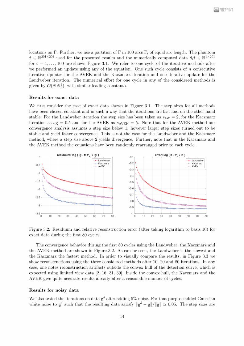
locations on Γ. Further, we use a partition of Γ in 100 arcs Γi of equal arc length. The phantomf ∈ R201×201 used for the presented results and the numerically computed data Mif ∈ R1×201

for i = 1, . . . , 100 are shown Figure 3.1. We refer to one cycle of the iterative methods afterwe performed an update using any of the equation. One such cycle consists of n consecutiveiterative updates for the AVEK and the Kaczmarz iteration and one iterative update for theLandweber iteration. The numerical effort for one cycle in any of the considered methods isgiven by O(NN2

x), with similar leading constants.

Results for exact data

We first consider the case of exact data shown in Figure 3.1. The step sizes for all methodshave been chosen constant and in such a way that the iterations are fast and on the other handstable. For the Landweber iteration the step size has been taken as sLW = 2, for the Kaczmarziteration as sK = 0.5 and for the AVEK as sAVEK = 5. Note that for the AVEK method ourconvergence analysis assumes a step size below 1; however larger step sizes turned out to bestable and yield faster convergence. This is not the case for the Landweber and the Kaczmarzmethod, where a step size above 2 yields divergence. Further, note that in the Kaczmarz andthe AVEK method the equations have been randomly rearranged prior to each cycle.

0 10 20 30 40 50 60 70 80

-3.5

-3

-2.5

-2

-1.5

-1

-0.5

0residuum: log ( |g - M fδ

k | / |g| )

Landweber

Kaczmarz

AVEK

0 10 20 30 40 50 60 70 80

-1

-0.9

-0.8

-0.7

-0.6

-0.5

-0.4

-0.3

-0.2

-0.1error: log ( |f - fδ

k| / |f| )

Landweber

Kaczmarz

AVEK

Figure 3.2: Residuum and relative reconstruction error (after taking logarithm to basis 10) forexact data during the first 80 cycles.

The convergence behavior during the first 80 cycles using the Landweber, the Kaczmarz andthe AVEK method are shown in Figure 3.2. As can be seen, the Landweber is the slowest andthe Kaczmarz the fastest method. In order to visually compare the results, in Figure 3.3 weshow reconstructions using the three considered methods after 10, 20 and 80 iterations. In anycase, one notes reconstruction artifacts outside the convex hull of the detection curve, which isexpected using limited view data [2, 16, 31, 39]. Inside the convex hull, the Kaczmarz and theAVEK give quite accurate results already after a reasonable number of cycles.

Results for noisy data

We also tested the iterations on data gδ after adding 5% noise. For that purpose added Gaussianwhite noise to gδ such that the resulting data satisfy ‖gδ − g‖/‖g‖ ≃ 0.05. The step sizes are

14

0

0.2

0.4

0.6

0.8

1

0

0.2

0.4

0.6

0.8

1

0

0.2

0.4

0.6

0.8

1

0

0.2

0.4

0.6

0.8

1

0

0.2

0.4

0.6

0.8

1

0

0.2

0.4

0.6

0.8

1

0

0.2

0.4

0.6

0.8

1

0

0.2

0.4

0.6

0.8

1

0

0.2

0.4

0.6

0.8

1

Figure 3.3: Reconstructions from exact data after 10 iterations (left), 20 iterations (center) and80 iterations (right). Top row: Landweber. Middle row: Kaczmarz. Bottom row: AVEK.

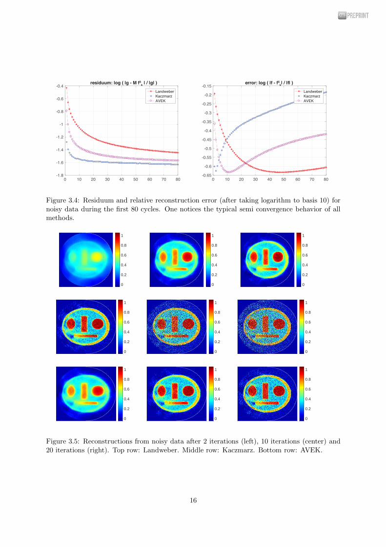
taken as in the exact data case and τk is chosen in such a way that no iterations are skipped.The convergence behavior during the first 80 cycles using noisy data is shown in Figure 3.4. Onenotes that as in the exact data case, the residuals ‖Mfδk−gδ‖ are decreasing for all methods. Thereconstruction errors ‖fδk − f‖, on the other hand, show the typical semi-convergence behaviorfor ill-posed problems. The Kaczmarz iteration is again the fastest and the Landweber methodagain the slowest method. The minimal L2-reconstruction errors have been obtained after 48iterations for the Landweber iteration, after 2 cycles for the Kaczmarz iteration, and after 11cycles for the AVEK. The corresponding relative reconstruction errors ‖fδk − f‖/‖f‖ are 0.2363for the Kaczmarz method and and 0.2327 for the Landweber as well as the AVEK method. TheLandweber and the AVEK method therefore slightly outperform the Kaczmarz method in termsof the minimal reconstruction error. Reconstruction results after 2, 10 and 20 iterations areshown in Figure 3.5.

As the results of iterative methods for inconsistent problems are known to essentially dependon the step size (for example of the Kaczmarz method [10, 32]), developing appropriate stepsize strategies can significantly improve the results. Here we have simply used constant andconservative step sizes. Further, adjusting the skipping parameters αk can potentially improveand stabilize the AVEK method. A precise comparison of the methods using parameter fine-tuning and implementing adaptive and data-driven choices deserves further investigation; this,however, is beyond the scope of this paper.

15

0 10 20 30 40 50 60 70 80

-1.8

-1.6

-1.4

-1.2

-1

-0.8

-0.6

-0.4residuum: log ( |g - M fδ

k | / |g| )

Landweber

Kaczmarz

AVEK

0 10 20 30 40 50 60 70 80

-0.65

-0.6

-0.55

-0.5

-0.45

-0.4

-0.35

-0.3

-0.25

-0.2

-0.15error: log ( |f - fδ

k| / |f| )

Landweber

Kaczmarz

AVEK

Figure 3.4: Residuum and relative reconstruction error (after taking logarithm to basis 10) fornoisy data during the first 80 cycles. One notices the typical semi convergence behavior of allmethods.

0

0.2

0.4

0.6

0.8

1

0

0.2

0.4

0.6

0.8

1

0

0.2

0.4

0.6

0.8

1

0

0.2

0.4

0.6

0.8

1

0

0.2

0.4

0.6

0.8

1

0

0.2

0.4

0.6

0.8

1

0

0.2

0.4

0.6

0.8

1

0

0.2

0.4

0.6

0.8

1

0

0.2

0.4

0.6

0.8

1

Figure 3.5: Reconstructions from noisy data after 2 iterations (left), 10 iterations (center) and20 iterations (right). Top row: Landweber. Middle row: Kaczmarz. Bottom row: AVEK.

16

4 Conclusion and outlook

In this paper we introduced the averaged Kaczmarz (AVEK) method as a paradigm of a newiterative regularization method. AVEK can be seen as a hybrid between Landweber’s andKaczmarz’s method for solving inverse problems given as systems of equations Fi(x) = yi. Asthe Kaczmarz method, AVEK requires only solving one forward and one adjoint problem periteration. As the Landweber method, it uses information from all equations per update whichcan have a stabilizing effect. As main theoretical results, we have shown that the AVEK methodconverges weakly in the case of exact data (see Theorem 2.6), and presented convergence resultsfor noisy data (see Theorem 2.9). Note that the convergence as δ → 0 in Theorem 2.9 (b)assumes strong convergence in the exact data case. It is an open problem if the same conclusionholds under its weak convergence only. Another open problem is the strong convergence forexact data in the general case. We conjecture both issues to hold true.

In Section 3, we presented numerical results for the AVEK method applied to the limited viewproblem for the circular Radon, which is relevant for photoacoustic tomography. For comparisonpurpose we also applied the Landweber and the Kaczmarz method to the same problem. In theexact data case, the observed convergence speed (number of cycles versus reconstruction error)of the AVEK turned out to be somewhere between the Kaczmarz (fastest) and the Landwebermethod (slowest). A similar behavior has been observed in the noisy data case. In this case,the minimal reconstruction error for the AVEK is slightly smaller that the one of the Kaczmarzmethod and equal to the Landweber method. The required number of iterations however is lessthan the one of the Landweber method. These initial results are encouraging and show thatthe AVEK is a useful iterative method for tomographic image reconstruction. Detailed studiesare required in future work on the optimal selection of parameter such as the step sizes or thenumber of partitions.

We see AVEK as the basic member of a new class of iterative reconstruction method. Itshares some similarities with the incremental gradient method proposed in the seminal work [7](studied for well-posed problems in finite dimensions). Applied to (1.1), the incremental gradientmethod reads

∀k ≥ n : xk+1 = xk −skn

k∑

ℓ=k−n+1

F′[ℓ](xℓ)

∗(F[ℓ](xℓ) − y[ℓ]) .

Instead of an average over individual auxiliary updates, the incremental gradient method uses anaverage over the individual gradients. Studying and analyzing the incremental gradient methodfor inverse problems is an interesting open issue. The incremental gradient method has beengeneralized in various directions. This includes proximal incremental gradient methods [5] orthe averaged stochastic gradient method of [37]. Similar extensions for the AVEK (for ill-posedas well as well-posed problems) are interesting lines of future research.

Acknowledgment

H.L. acknowledges support through the National Nature Science Foundation of China (61571008,61402495).

17

A Deconvolution of sequences and proof of Lemma 2.5

The main aim of this appendix is to prove Lemma 2.5, concerning the convergence of thedifference of two consecutive iterates of the AVEK iteration. For that purpose, we will firstderive auxiliary results concerning deconvolution equations for sequences in Hilbert spaces thatare of interest in its own.

For the following it is helpful to identify any sequence (ak)k∈N0 ∈ CN0 with a formal powerseries a =

∑∞k=0 akX

k. Here Xk ∈ CN0 is the sequence defined by Xkk = 1 and Xk

ℓ = 0 forℓ 6= k. For two complex sequences a, b ∈ CN0 , the Cauchy product a ∗ b ∈ CN0 is defined by(a ∗ b)k :=

∑kj=0 ajbk−j; see [20]. We say that a ∈ CN0 is invertible if there is b ∈ CN0 with

a ∗ b = (1, 0, . . . ). We write b := a−1 and call it the reciprocal formal power series of a, orsimply the inverse of a. Moreover one easily verifies (see [20]) that the formal power seriesa =

∑∞k=0 akX

k is invertible if and only if a0 6= 0. In this case b = a−1 is unique and defined

by the recursion b0 = 1/a0 and bk = − 1a0

∑k−1j=0 bjak−j for k ≥ 1. One further verifies that CN0

together with point-wise addition and scalar multiplication and the Cauchy product forms anassociative algebra.

A.1 Convolutions in Hilbert spaces

Throughout this subsection X denotes an arbitrary Hilbert space. For a ∈ CN0 and x ∈ XN0

define the convolution x ∗ a ∈ XN0 by

∀k ∈ N0 : (x ∗ a)k :=

k∑

j=0

xjak−j . (A.1)

One verifies that (x∗a)∗b = x∗(a∗b) for a, b ∈ CN0 and x ∈ XN0 . Moreover, the set of boundedsequences ℓ∞(N0,X) := {x ∈ XN0 | xk bounded} forms a Banach space together with thesupremum norm ‖x‖∞ := sup{‖xk‖ | k ∈ N0}. Finally, c0(N0,X) := {x ∈ XN0 | limk→∞ xk = 0}denotes the space of sequences in X converging to zero.

Lemma A.1. Let b ∈ ℓ1(N0,C) and define b(m) := (b0, . . . , bm, 0, . . . ). Then,

(a) ∀x ∈ c0(N0,X) : x ∗ b(m) ∈ c0(N0,X);

(b) ∀x ∈ ℓ∞(N0,X) : x ∗ b ∈ ℓ∞(N0,X) ∧ limm→∞ ‖x ∗ b− x ∗ b(m)‖∞ = 0;

(c) ∀x ∈ c0(N0,X) : x ∗ b ∈ c0(N0,X).

Proof. (a) For k ≥ m we have (x ∗ b(m))k =∑k

j=0 xjbk−j =∑k

j=k−m xjbk−j. Hence x ∗ b(m)

converges to zero because xjbk−j does so.

(b) For k ≤ m we have (x ∗ b(m))k =∑k

j=0 xjbk−j = (x ∗ b)k. For k > m we have

� (x ∗ b)k − (x ∗ b(m))k =∑k

j=0 xjbk−j −∑k

j=k−mxjbk−j =∑k−m−1

j=0 xjbk−j;

� ‖(x ∗ b)k − (x ∗ b(m))k‖ ≤ ‖x‖∞∑k−m−1

j=0 |bk−j| ≤ ‖x‖∞∑∞

j=m+1 |bj|;

�∑∞

j=m+1 |bj| → 0 (because∑

k∈N0|bk| < ∞).

We conclude that ‖(x ∗ b) − (x ∗ b(m))‖∞ ≤ ‖x‖∞∑∞

j=m+1 |bj | → 0.(c) Follows from (a), (b) and the closedness of c0(N0,X) in ℓ∞(N0,X).

18

As an application of Lemma A.1 we can show the following result, which is the main ingre-dient for the proof of Lemma 2.5.

Proposition A.2 (A deconvolution problem). For any sequence d = (dk)∞k=1 in XN0 and anyn ∈ N0, the following implication holds true:

limk→∞

n∑

j=1

jdk−n+j = 0 =⇒ limk→∞

dk = 0 .

Proof. Set a := (n, n − 1, . . . , 1, 0, . . . ) and suppose that (d ∗ a)k → 0 as k → ∞. We have toverify that dk → 0 as k → ∞, which is divided in several steps.

� Step 1: All zeros of the polynomial p : C → C : z 7→ n + (n− 1)z + · · · zn−1 are containedin {z ∈ C | ‖z‖ > 1}.

Because p(0) 6= 0, in order to verify Step 1, it is sufficient to show that all zeros of p(1/z)are contained in the unit disc B1(0) = {z ∈ C | ‖z‖ < 1}. Hence it is sufficient to show that thepolynomial q(z) := zn−1p(1/z) := nzn−1+(n−1)zn−2+· · ·+1 has all zeros in B1(0). Further notethat q(z) = Q′(z), where Q(z) := zn + zn−1 + · · ·+ z has the form Q(z) = z zn−1

z−1 . Consequently,{0} ∪ {z ∈ C | zn = 1 ∧ z 6= 1} is the set of zeros of Q. The Gauss-Lukas theorem (see [28,Theorem (6,1)]) states that all critical points of a non-constant polynomial f are contained inthe convex hull H of the set of zeros of f . If the zeros of f are not collinear, then no critical pointlies on ∂H unless it is a multiple zero of f . Note that all zeros of Q are simple, not collinearand contained in B1(0). According the Gauss-Lukas theorem all zeros of q = Q′ are containedin B1(0). Consequently all zeros of p are indeed contained in {z ∈ C | ‖z‖ > 1}.

� Step 2: We have a−1 ∈ ℓ1(N0,C).

All zeros of p(z) are outside of B1+ǫ(0) for some ǫ > 0 and therefore 1/p(z) is analytic inB1+ǫ(0) and can be expanded in a power series 1/p(z) =

∑k∈N0

bkzk. The radius of convergence

is at least 1 + ǫ (as the radius of convergence of a function f is the radius of the largest discwhere f or an analytic continuation of f is analytic; see for example [20, Theorem 3.3a].) Wehave

1 = p(z)1

p(z)=

n−1∑

j=0

ajzj∑

k∈N0

bkzk =

∑

k∈N0

(a ∗ b)kzk .

Hence a ∗ b = (1, 0, 0, . . . ) and a−1 = b ∈ ℓ1(N0,C).

� Step 3: We are now ready to complete the proof. According to the assumption, we haved ∗ a ∈ c0(N0,X). According to Step 2, we have a−1 ∈ ℓ1(N0,C). Therefore Lemma A.1 (c)implies that d = (d ∗ a) ∗ a−1 ∈ c0(N0,X).

A.2 Application to the AVEK iteration

Now let xk is defined by (2.4), let x∗ ∈ Bρ(x0) be an arbitrary solution to (1.1) and assumethat (2.1) and (2.2) hold true. We introduce the auxiliary sequences dk := xk+1 − xk, zk :=1n

∑nj=1 jxk−n+j and rk := F′

[k](xk)∗(F[k](xk) − y[k]). Here dk are the differences between twoconsecutive iterations that we show to converge to zero, zk will be required in the subsequentanalysis, and rk are the residuals.

19

Lemma A.3.

(a) limk→∞xk+1 − 1/n∑k

l=k−n+1xℓ = 0;

(b) zk+1 − zk = xk+1 − 1/n∑k

ℓ=k−n+1 xℓ;

(c) limk→∞ zk+1 − zk = 1/n limk→∞∑n

j=1 jdk−n+j = 0.

Proof. (a): By the definition of xk, rk we have xk+1 = 1n

∑kℓ=k−n+1 xℓ − sℓrℓ. Therefore

∥∥∥xk+1 −1

n

k∑

l=k−n+1

xℓ

∥∥∥ =∥∥∥ 1

n

k∑

ℓ=k−n+1

sℓrℓ

∥∥∥ ≤ 1

n

k∑

ℓ=k−n+1

sℓ‖rℓ‖ .

As we already know that sℓ‖rℓ‖ → 0, the claim follows.(b): We have

zk+1 − zk =1

n

n∑

j=1

jxk−n+j+1 −1

n

n∑

j=1

jxk−n+j

= xn+1 +1

n

n−1∑

j=1

jxk−n+j+1 −1

n

n∑

j=2

jxk−n+j −1

nxk−n+1

= xn+1 +1

n

n∑

j=2

(j − 1)xk−n+j −1

n

n∑

j=2

jxk−n+j −1

nxk−n+1

= xn+1 −1

n

n∑

j=2

xk−n+j −1

nxk−n+1 = xn+1 −

1

n

n∑

j=1

xk−n+j .

(c): Follows from (a), (b).

Proof of Lemma 2.5

Lemma 2.5 now is an immediate consequence of Lemma A.3 and Proposition A.2. In fact, fromLemma A.3 (c) we know that limk→∞

∑nj=1 jdk−n+j = 0 for k → ∞. Then the assertion follows

from Proposition A.2.

References

[1] L.-E. Andersson. On the determination of a function from spherical averages. SIAM J.Appl. Math., 19(1):214–232, 1988.

[2] L. L. Barannyk, J. Frikel, and L. V. Nguyen. On artifacts in limited data spherical Radontransform: curved observation surface. Inverse Probl., 32(1):015012, 32, 2016.

[3] J. Baumeister, B. Kaltenbacher, and A. Leitao. On Levenberg-Marquardt-Kaczmarz itera-tive methods for solving systems of nonlinear ill-posed equations. Inverse Probl. Imaging,4(3):335–350, 2010.

[4] A. Beltukov and D. Feldman. Identities among Euclidean Sonar and Radon transforms.Adv. in Appl. Math., 42(1):23–41, 2009.

20

[5] Dimitri P. Bertsekas. Incremental proximal methods for large scale convex optimization.Math. Program., 129(2, Ser. B):163–195, 2011.

[6] B. Blaschke, A. Neubauer, and O. Scherzer. On convergence rates for the iteratively regu-larized Gauss-Newton method. IMA J. Numer. Anal., 17(3):421–436, 1997.

[7] Doron Blatt, Alfred O Hero, and Hillel Gauchman. A convergent incremental gradientmethod with a constant step size. SIAM J. Optim., 18(1):29–51, 2007.

[8] N. Bleistein, J. K. Cohen, and J. W. Stockwell, Jr. Mathematics of multidimensional seismicimaging, migration, and inversion, volume 13 of Interdisciplinary Applied Mathematics.Springer-Verlag, New York, 2001. Geophysics and Planetary Sciences.

[9] P. Burgholzer, J. Bauer-Marschallinger, H. Grun, M. Haltmeier, and G. Paltauf. Temporalback-projection algorithms for photoacoustic tomography with integrating line detectors.Inverse Probl., 23:S65, 2007.

[10] Y. Censor, P. P. B. Eggermont, and D. Gordon. Strong underrelaxation in Kaczmarz’smethod for inconsistent systems. Numer. Math., 41(1):83–92, 1983.

[11] A. De Cezaro, M. Haltmeier, A. Leitao, and O. Scherzer. On steepest-descent-Kaczmarzmethods for regularizing systems of nonlinear ill-posed equations. Appl. Math. Comput.,202(2):596–607, 2008.

[12] Herbert Egger and Andreas Neubauer. Preconditioning Landweber iteration in Hilbertscales. Numer. Math., 101(4):643–662, 2005.

[13] Tommy Elfving, Per Christian Hansen, and Touraj Nikazad. Convergence analysis forcolumn-action methods in image reconstruction. Numer. Algorithms, 74(3):905–924, 2017.

[14] H. W. Engl, M. Hanke, and A. Neubauer. Regularization of inverse problems, volume 375of Mathematics and its Applications. Kluwer Academic Publishers Group, Dordrecht, 1996.

[15] D. Finch, M. Haltmeier, and Rakesh. Inversion of spherical means and the wave equationin even dimensions. SIAM J. Appl. Math., 68(2):392–412, 2007.

[16] J. Frikel and E. T. Quinto. Artifacts in incomplete data tomography with applications tophotoacoustic tomography and sonar. SIAM J. Appl. Math., 75(2):703–725, 2015.

[17] M. Haltmeier, R. Kowar, A. Leitao, and O. Scherzer. Kaczmarz methods for regularizingnonlinear ill-posed equations. II. Applications. Inverse Probl. Imaging, 1(3):507–523, 2007.

[18] M. Haltmeier, A. Leitao, and O. Scherzer. Kaczmarz methods for regularizing nonlinearill-posed equations. I. Convergence analysis. Inverse Probl. Imaging, 1(2):289–298, 2007.

[19] M. Hanke, A. Neubauer, and O. Scherzer. A convergence analysis of the Landweber iterationfor nonlinear ill-posed problems. Numer. Math., 72(1):21–37, 1995.

[20] P. Henrici. Applied and computational complex analysis, volume 1. Wiley-Interscience, NewYork-London-Sydney, 1974.

21

[21] B. Kaltenbacher, A. Neubauer, and O. Scherzer. Iterative regularization methods for non-linear ill-posed problems, volume 6 of Radon Series on Computational and Applied Mathe-matics. Walter de Gruyter GmbH & Co. KG, Berlin, 2008.

[22] Stefan Kindermann and Antonio Leitao. Convergence rates for Kaczmarz-type regulariza-tion methods. Inverse Probl. Imaging, 8(1):149–172, 2014.

[23] R. Kowar and O. Scherzer. Convergence analysis of a Landweber-Kaczmarz method forsolving nonlinear ill-posed problems. In Ill-posed and inverse problems, pages 253–270.VSP, Zeist, 2002.

[24] P. Kuchment and L. Kunyansky. Mathematics of photoacoustic and thermoacoustic to-mography. In Handbook of Mathematical Methods in Imaging, pages 817–865. Springer,2011.

[25] L. Landweber. An iteration formula for Fredholm integral equations of the first kind. Amer.J. Math., 73:615–624, 1951.

[26] A. Leitao and B. F. Svaiter. On projective Landweber-Kaczmarz methods for solvingsystems of nonlinear ill-posed equations. Inverse Probl., 32(2):025004, 20, 2016.

[27] Z. Q. Luo. On the convergence of the lms algorithm with adaptive learning rate for linearfeedforward networks. Neural Comput., 3(2):226–245, June 1991.

[28] M. Marden. Geometry of polynomials. Second edition. Mathematical Surveys, No. 3. Amer-ican Mathematical Society, Providence, R.I., 1966.

[29] F. Natterer and F. Wubbeling. Mathematical Methods in Image Reconstruction, volume 5 ofMonographs on Mathematical Modeling and Computation. SIAM, Philadelphia, PA, 2001.

[30] A. Neubauer and O. Scherzer. A convergence rate result for a steepest descent methodand a minimal error method for the solution of nonlinear ill-posed problems. Z. Anal.Anwendungen, 14(2):369–377, 1995.

[31] Linh V. Nguyen. On artifacts in limited data spherical Radon transform: flat observationsurfaces. SIAM J. Math. Anal., 47(4):2984–3004, 2015.

[32] Touraj Nikazad, Mokhtar Abbasi, and Tommy Elfving. Error minimizing relaxation strate-gies in Landweber and Kaczmarz type iterations. J. Inverse Ill-Posed Probl., 25(1):35–56,2017.

[33] S. J. Norton and M. Linzer. Ultrasonic reflectivity imaging in three dimensions: Exactinverse scattering solutions for plane, cylindrical and spherical apertures. IEEE Trans.Biomed. Eng., 28(2):202–220, 1981.

[34] Zdzis l aw Opial. Weak convergence of the sequence of successive approximations for non-expansive mappings. Bull. Amer. Math. Soc., 73:591–597, 1967.

[35] Andreas Rieder. On the regularization of nonlinear ill-posed problems via inexact Newtoniterations. Inverse Probl., 15(1):309–327, 1999.

22

[36] O. Scherzer, M. Grasmair, H. Grossauer, M. Haltmeier, and F. Lenzen. Variational methodsin imaging, volume 167 of Applied Mathematical Sciences. Springer, New York, 2009.

[37] M. Schmidt, N. Le Roux, and F. Bach. Minimizing finite sums with the stochastic averagegradient. Math. Program., 162(1-2):83–112, 2017.

[38] M. V. Solodov. Incremental gradient algorithms with stepsizes bounded away from zero.Comput. Optim. Appl., 11(1):23–35, 1998.

[39] P. Stefanov and G. Uhlmann. Is a curved flight path in SAR better than a straight one?SIAM J. Appl. Math., 73(4):1596–1612, 2013.

[40] K. Wang, R. W. Schoonover, R. Su, A. Oraevsky, and M. A. Anastasio. Discrete imagingmodels for three-dimensional optoacoustic tomography using radially symmetric expansionfunctions. IEEE Trans. Med. Imag., 33(5):1180–1193, 2014.

[41] M. Xu and L. V. Wang. Universal back-projection algorithm for photoacoustic computedtomography. Phys. Rev. E, 71(1):016706, 2005.

[42] G. Zangerl, O. Scherzer, and M. Haltmeier. Exact series reconstruction in photoacoustictomography with circular integrating detectors. Commun. Math. Sci., 7(3):665–678, 2009.

23