VIII Seasonal Adjustment and Estimation of Trend-Cycles · PDF fileVIII Seasonal Adjustment...

125

VIII Seasonal Adjustment and Estimation of Trend-Cycles

A. Introduction

8.1. Seasonal adjustment serves to facilitate anunderstanding of the development of the economyover time, that is, the direction and magnitude ofchanges that have taken place. Such understandingcan be best pursued through the analyses of timeseries.1 One major reason for compiling high-fre-quency statistics such as GDP is to allow timely iden-tification of changes in the business cycle,particularly turning points. If observations of, say,quarterly non-seasonally adjusted GDP at constantprices are put together for consecutive quarters cov-ering several years to form a time series and aregraphed, however, it is often difficult to identify turn-ing points and the underlying direction of the data.The most obvious pattern in the data may be a recur-rent within-a-year pattern, commonly referred to asthe seasonal pattern.

8.2. Seasonal adjustment means using analyticaltechniques to break down a series into its compo-nents. The purpose is to identify the different compo-nents of the time series and thus provide a betterunderstanding of the behavior of the time series. Inseasonally adjusted data, the impact of the regularwithin-a-year seasonal pattern, the influences ofmoving holidays such as Easter and Ramadan, andthe number of working/trading days and the weekdaycomposition in each period (the trading-day effect,for short) are removed. By removing the repeatedimpact of these effects, seasonally adjusted datahighlight the underlying trends and short-run move-ments in the series.

8.3. In trend-cycle estimates, the impact of irregularevents in addition to seasonal variations is removed.

Adjusting a series for seasonal variations removes theidentifiable, regularly repeated influences on theseries but not the impact of any irregular events.Consequently, if the impact of irregular events isstrong, seasonally adjusted series may not represent asmooth, easily interpretable series. To further high-light the underlying trend-cycle, most standard sea-sonal adjustment packages provide a smoothed trendline running through the seasonally adjusted data(representing a combined estimate of the underlyinglong-term trend and the business-cycle movements inthe series).

8.4. An apparent solution to get around seasonal pat-terns would be to look at rates of change from thesame quarter of the previous year. This has the disad-vantage, however, that turning points are onlydetected with some delay.2 Furthermore, these ratesof change do not fully exclude all seasonal elements(e.g., Easter may fall in the first or second quarter,and the number of working days of a quarter may dif-fer between succeeding years). Moreover, these year-to-year rates of change will be biased owing tochanges in the seasonal pattern caused by institu-tional or behavioral changes. Finally, these year-to-year rates of change will reflect any irregular eventsaffecting the data for the same period of the previousyear in addition to any irregular events affecting thecurrent period. For these reasons, year-to-year ratesof change are inadequate for business-cycle analysis.

8.5. Therefore, more sophisticated procedures areneeded to remove seasonal patterns from the series.Various well-established techniques are available forthis purpose. The most commonly used technique isthe Census X-11/X-12 method. Other available sea-sonal adjustment methods include, among others,TRAMO-SEATS, BV4, SABLE, and STAMP.

1Paragraph 1.13 defined time series as a series of data obtainedthrough repeated measurement of the same concept over time thatallows different periods to be compared.

2The delay can be substantial, on average, two quarters. A numericalexample illustrating this point is provided in Annex 1.1.

8.6. A short presentation on the basic concept ofseasonal adjustment is given in Section B of thischapter, while the basic principles of the CensusX-11/X-12 method are outlined in section C. Thefinal section, Section D, addresses a series ofrelated general seasonal adjustment issues, such asrevisions to the seasonally adjusted data and thewagging tail problem, and the minimum length oftime series for seasonal adjustment. Section D alsoaddresses a set of critical issues on seasonal adjust-ment of quarterly national accounts (QNA), such aspreservation of accounting identities, seasonaladjustment of balancing items and aggregates, andthe relationship between annual data and season-ally adjusted quarterly data. Section D also dis-cusses the presentation and status of seasonallyadjusted and trend-cycle data.

B. The Main Principles of SeasonalAdjustment

8.7. For the purpose of seasonal adjustment, a timeseries is generally considered to be made up ofthree main components—the trend-cycle compo-nent, the seasonal component, and the irregularcomponent—each of which may be made up of sev-eral subcomponents:(a) The trend-cycle (Tt) component is the underlying

path or general direction reflected in the data, thatis, the combined long-term trend and the busi-ness-cycle movements in the data.

(b) The seasonal (Sct ) component includes seasonal

effects narrowly defined and calendar-related sys-tematic effects that are not stable in annual tim-ing, such as trading-day effects and movingholiday effects.(i) The seasonal effect narrowly defined (St) is an

effect that is reasonably stable3 in terms ofannual timing, direction, and magnitude.Possible causes for the effect are natural factors,administrative or legal measures, social/culturaltraditions, and calendar-related effects that arestable in annual timing (e.g., public holidayssuch as Christmas).

(ii) Calendar-related systematic effects on thetime series that are not stable in annual timingare caused by variations in the calendar fromyear to year. They include the following:� The trading-day effect (TDt), which is

the effect of variations from year to yearin the number working, or trading, daysand the weekday composition for a par-ticular month or quarter relative to thestandard for that particular month orquarter.4,5

� The effects of events that occur at regu-lar intervals but not at exactly the sametime each year, such as moving holidays(MHt), or paydays for large groups ofemployees, pension payments, and soon.

� Other calendar effects (OCt), such as leap-year and length-of-quarter effects.

� Both the seasonal effects narrowly definedand the other calendar-related effects rep-resent systematic, persistent, predictable,and identifiable effects.

(c) The irregular component (Ict ) captures effects that

are unpredictable unless additional information isavailable, in terms of timing, impact, and dura-tion. The irregular component (Ic

t ) includes thefollowing:(i) Irregular effects narrowly defined (It).(ii) Outlier6 effects (OUTt).(iii) Other irregular effects (OIt) (such as the

effects of unseasonable weather, naturaldisasters, strikes, and irregular salescampaigns).

The irregular effect narrowly defined is assumed tobehave as a stochastic variable that is symmetri-cally distributed around its expected value (0 for anadditive model and 1 for a multiplicative model).

VIII SEASONAL ADJUSTMENT AND ESTIMATION OF TREND-CYCLES

126

3It may be gradually changing over time (moving seasonality).

4The period-to-period variation in the standard, or average, numberand type of trading days for each particular month or quarter of theyear is part of the seasonal effect narrowly defined.5Trading-day effects are less important in quarterly data than inmonthly data but can still be a factor that makes a difference.6That is, an unusually large or small observation, caused by either toerrors in the data or special events, which may interfere with estimat-ing the seasonal factors.

8.8. The relationship between the original seriesand its trend-cycle, seasonal, and irregular compo-nents can be modeled as additive or multiplicative.7

That is, the time-series model can be expressed as

Additive Model

Xt = Sct + Tt + Ic

t (8.1.a)

or with some subcomponents specified

Xt = (St + TDt + MHt + OCt) + Tt + (It + OUTt + OIt) (8.1.b)

where

the seasonal component is Sc

t = (St + TDt + MHt + OCt)

the irregular component is Ic

t = (It + OUTt + OIt), and

the seasonally adjusted series is At = Tt + Ic

t = Tt + (It + OUTt + OIt ) ,

or as

Multiplicative Model

Xt = Sct + Tt + Ic

t (8.2.a)

or with some subcomponents specified Xt = (St

• TDt• MHt

• OCt) • Tt• (It

• OUTt• OIt) (8.2.b)

where

the seasonal component is Sct = (St

• TDt• MHt

• OCt),

the irregular component is Ict = (It

• OUTt• OIt), and

the seasonally adjusted series is At = Tt

• Ict = Tt

• (It• OUTt

• OIt).

8.9. The multiplicative model is generally taken as thedefault. The model assumes that the absolute size of thecomponents of the series are dependent on each otherand thus that the seasonal oscillation size increases and

decreases with the level of the series, a characteristic ofmost seasonal macroeconomic series. With the multi-plicative model, the seasonal and irregular componentswill be ratios centered around 1. In contrast, the addi-tive model assumes that the absolute size of the com-ponents of the series are independent of each other and,in particular, that the size of the seasonal oscillations isindependent of the level of the series.

8.10. Seasonal adjustment means using analyticaltechniques to break down a series into its components.The purpose is to identify the different components ofthe time series and thus to provide a better understand-ing of the behavior of the time series for modeling andforecasting purposes, and to remove the regular within-a-year seasonal pattern to highlight the underlyingtrends and short-run movements in the series. The pur-pose is not to smooth the series, which is the objectiveof trend and trend-cycle estimates. A seasonallyadjusted series consists of the trend-cycle plus the irreg-ular component and thus, as noted in the introduction,if the irregular component is strong, may not representa smooth easily interpretable series.

8.11. Example 8.1 presents the last four years of a timeseries and provides an illustration of what is meant byseasonal adjustment, the trend-cycle component, theseasonal component, and the irregular component.

8.12. Seasonal adjustment and trend-cycle estima-tion represent an analytical massaging of the originaldata. As such, the seasonally adjusted data and theestimated trend-cycle component complement theoriginal data, but, as explained in Section D ofChapter I, they can never replace the original data forthe following reasons:• Unadjusted data are useful in their own right. The

non-seasonally adjusted data show the actual eco-nomic events that have occurred, while the season-ally adjusted data and the trend-cycle estimaterepresent an analytical elaboration of the datadesigned to show the underlying movements thatmay be hidden by the seasonal variations.Compilation of seasonally adjusted data, exclu-sively, represents a loss of information.

• No unique solution exists on how to conduct sea-sonal adjustment.

• Seasonally adjusted data are subject to revisions asfuture data become available, even when the origi-nal data are not revised.

• When compiling QNA, balancing and reconcilingthe accounts are better done on the original unad-justed QNA estimates.

The Main Principles of Seasonal Adjustment

127

7Other main alternatives exist, in particular, X-12-ARIMA includes apseudo-additive model Xt = Tt • (Sc

t + Ict – 1) tailored to series whose

value is zero for some periods. Moreover, within each of the mainmodels, the relationship between some of the subcomponentsdepends on the exact estimation routine used. For instance, in themultiplicative model, some of the sub-components may beexpressed as additive to the irregular effect narrowly defined, e.g., as:Xt = St • Tt • (It + OUTt + OIt + TRt + MHt + OCt).


128

Example 8.1. Seasonal Adjustment,Trend-Cycle Component, Seasonal Component, andIrregular Component

Multiplicative Seasonal Model

Unadjusted Seasonally Adjusted Trend-CycleTime Series Series Component

(Xt) Seasonal Factors1 Irregular Component (Xt /St) (Tt)Index 1980 = 100 (St) (It) Index 1980 = 100 Index 1980 = 100

Date (1) (2) (3) (4) = (1)/(2) (5) = (4)/(3)q1 1996 138.5 0.990 1.005 139.8 139.2q2 1996 138.7 1.030 0.996 134.6 135.2q3 1996 133.6 1.024 1.003 130.5 130.1q4 1996 120.9 0.962 1.000 125.7 125.7q1 1997 120.9 0.981 0.993 123.2 124.2q2 1998 130.6 1.027 1.002 127.2 126.9q3 1997 134.4 1.033 1.005 130.1 129.4q4 1997 124.5 0.964 0.994 129.1 129.9q1 1998 127.7 0.975 1.001 131.0 130.8q2 1998 135.0 1.023 1.003 131.9 131.5q3 1998 135.6 1.037 0.993 130.7 131.6q4 1998 132.1 0.968 1.035 136.4 131.8q1 1999 127.6 0.971 0.998 131.5 131.7q2 1999 134.6 1.020 0.997 131.9 132.4q3 1999 142.1 1.041 1.015 136.5 134.4q4 1999 131.5 0.970 0.999 135.5 135.7q1 2000 132.1 0.969 1.000 136.3 136.3With a multiplicative seasonal model, the seasonal factors are ratios centered around 1 and are reasonably stable in terms of annual timing, direction, and mag-nitude. The irregulars2 are also centered around 1 but with erratic oscillations.

Observe the particularly strong irregular effect, or outlier, for q4 1998. Examples 8.3 and 8.4 show how an outlier like this causes trouble in early identifica-tion of changes in the trend-cycle.1The values of the estimated seasonal component, particularly from the multiplicative model, are often called “seasonal factors.”2The irregular component is often referred to as “the irregulars,” and the seasonal component is often referred to as “the seasonals.”

120

125

130

135

140

1996 1997 1998 1999 2000

1996 1997 1998 1999 2000

1996 1997 1998 1999 2000

1996 1997 1998 1999 2000

1996 1997 1998 1999 2000

1996 1997 1998 1999 2000

Unadjusted time series Seasonally adjusted seriesSeasonally adjusted series and trend-cycle component

Irregular component

120

125

130

135

140

120

125

130

135

140

120

125

130

135

140

0.95

1.00

1.05

0.95

1.00

1.05

Seasonally adjusted series

Trend cycle component

Trend component Seasonal factors

• While errors in the source data may be more easilydetected from seasonally adjusted data, it may beeasier to identify the source for the errors and correctthe errors working with the unadjusted data.

• Practice has shown that seasonally adjusting the dataat the detailed level needed for compiling QNA esti-mates can leave residual seasonality in the aggregates.

The original unadjusted QNA estimates, the seasonallyadjusted estimates, and the trend-cycle component allprovide useful information about the economy (see Box1.1), and, for the major national accounts aggregates, allthree sets of data should be presented to the users.

8.13. Seasonal adjustment is normally done usingoff-the-shelf programs—most commonly worldwideby one of the programs in the X-11 family. Other pro-grams in common use include the TRAMO-SEATSpackage developed by Bank of Spain and promotedby Eurostat and the German BV4 program. The orig-inal X-11 program was developed in the 1960s by theU.S. Bureau of the Census. It has subsequently beenupdated and improved through the development ofX-11-ARIMA8 by Statistics Canada9 and X-12-ARIMA by the U.S. Bureau of the Census, whichwas released in the second half of the 1990s. The coreof X-11-ARIMA and X-12-ARIMA is the same basicfiltering procedure as in the original X-11.10

8.14. For particular series, substantial experience andexpertise may be required to determine whether theseasonal adjustment is done properly or to fine-tunethe seasonal adjustment. In particularly unstable serieswith a strong irregular component (e.g., outliers owingto strikes and other special events, breaks, or levelshifts), it may be difficult to seasonally adjust properly.

8.15. It is also important to emphasize, however, thatmany series are well-behaved and easy to seasonallyadjust, allowing seasonal adjustment programs to beused without specialized seasonal adjustment expertise.

The X-11 seasonal adjustment procedure has in practiceproved to be quite robust, and a large number of the sea-sonally adjusted series published by different agenciesaround the world are adjusted by running the programsin their default modes, often without special expertise.Thus, lack of experience in seasonal adjustment or lackof staff with particular expertise in seasonal adjustmentshould not preclude one from starting to compile andpublish seasonally adjusted estimates. When compilingseasonally adjusted estimates for the first time, however,keep in mind that the main focus of compilation and pre-sentation should be on the original unadjusted esti-mates. Over time, staff will gain experience andexpertise in seasonal adjustment.

8.16. It is generally recommended that the statisticianswho compile the statistics should also be responsible—either solely or together with seasonal adjustmentspecialists—for seasonally adjusting the statistics. Thisarrangement should give them greater insight into thedata, make their job more interesting, help them under-stand the nature of the data better, and lead to improvedquality of both the original unadjusted data and the sea-sonally adjusted data. However, it is advisable in addi-tion to set up a small central group of seasonaladjustment experts, because the in-depth seasonaladjustment expertise required to handle ill-behavedseries can only be acquired by hands-on experience withseasonal adjustment of many different types of series.

C. Basic Features of the X-11 Family ofSeasonal Adjustment Programs

8.17. The three programs in the X-11 family—X-11,X-11-ARIMA, and X-12-ARIMA— follow an itera-tive estimation procedure, the core of which is based ona series of moving averages.11 The programs compriseseven main parts in three main blocks of operations.First (part A), the series may optionally be “pread-justed” for outliers, level shifts in the series, the effectof known irregular events, and calendar-related effectsusing adjustment factors supplied by the user or esti-mated using built-in estimation procedures. In addition,the series may be extended by backcasts and forecastsso that less asymmetric filters can be used at the begin-ning and end of the series. Second (parts B, C, and D),the preadjusted series then goes through three rounds ofseasonal filtering and extreme value adjustments, the“B, C, and D iterations” in the X-11/X-12 jargon. Third

Basic Features of the X-11 Family of Seasonal Adjustment Programs

129

8Autoregressive integrated moving average time-series models.ARIMA modeling represents an optional feature in X-11-ARIMAand X-12-ARIMA to backcast and forecast the series so that lessasymmetric filters than in the original X-11 program can be used atthe beginning and end of the series (see paragraph. 8.37).9Initially released in 1980, with a major update in 1988, the X-11-ARIMA/88.10The X-12-ARIMA can be obtained by contacting the U.S. Bureauof the Census (as of the time of writing, X-12-ARIMA was availablefree and could be downloaded with complete documentation andsome discussion papers from http://www.census.gov/pub/ts/x12a/).X-11-ARIMA can be obtained by contacting Statistics Canada, andTRAMO-SEATS can be obtained by contacting Eurostat. The origi-nal X-11 program is integrated into several commercially availablesoftware packages (including among others SAS, AREMOS, andSTATSTICA).

11Also called “moving average filters” in the seasonal adjustmentterminology.

(parts E, F, and G), various diagnostics and quality con-trol statistics are computed, tabulated, and graphed.12

8.18. The second block—with the parts B, C, and Dseasonal filtering procedure—represents the central(X-11) core of the programs. The filtering procedure isbasically the same for all three programs. X-12-ARIMA, however, provides several new adjustmentoptions for the B, C, and D iterations that significantlyenhance this part of the program. The main enhance-ments made in X-12-ARIMA to the central X-11 partof the program include, among others, a pseudo-additive Xt = Tt • (Sc

t + Ict – 1) model tailored to series

whose value is zero for some periods; new centered sea-sonal and trend MA filters (see next section); improve-ments in how trading-day effects and other regressioneffects—including user-defined effects (a new capabil-ity)—are estimated from preliminary estimates of theirregular component (see Subsection 3 below).

8.19. In contrast, the first block, and to some extentthe last block (see Subsection 4), differ markedlyamong the three programs. The original X-11 providedno built-in estimation procedures for preadjustmentsof the original series besides trading-day adjustmentsbased on regression of tentative irregulars in parts Band C (see Subsection 1), but it provided for user-sup-plied permanent or temporary adjustment factors. X-11-ARIMA, in addition, provided for built-inprocedures for ARIMA-model-based backcasts andforecasts of the series. In contrast, X-12-ARIMA con-tains an extensive time-series modeling block, theRegARIMA part of the program, that allows the userto preadjust, as well as backcasts and forecasts of theseries by modeling the original series. The main com-ponents of X-12-ARIMA are shown in Box 8.1.

8.20. The RegARIMA block of the X-12-ARIMAallows the user to conduct regression analysis directlyon the original series, taking into account that the non-explained part of the series typically will be autocorre-lated, nonstationary, and heteroscedastic. This is doneby combining traditional regression techniques withARIMA modeling into what is labeled RegARIMAmodeling.13 The RegARIMA part of X-12-ARIMAallows the user to provide a set of user-defined

regressor variables. In addition, the program contains alarge set of predefined regressor variables to identify,for example, trading-day effects, Easter effects,14 leap-year effects, length-of-quarter effects, level shifts, pointoutliers, and ramps in the series. As a simpler alterna-tive to RegARIMA modeling, X-12-ARIMA hasretained the traditional X-11 approach of regressing thetentative irregulars on explanatory variables, addingregressors for point outliers and facilities for user-defined regressors to X-11’s trading-day and Eastereffects (see Subsection 3).

1. Main Aspects of the Core X-11 Moving AverageSeasonal Adjustment Filters

8.21. This subsection presents the main elements ofthe centered moving average filtering procedure in theX-12-ARIMA B, C, and D iterations for estimating thetrend-cycle component and the seasonal effects nar-rowly defined. The moving average filtering procedureimplicitly assumes that all effects except the seasonaleffects narrowly defined are approximately symmetri-cally distributed around their expected value (1 for amultiplicative and 0 for an additive model) and thuscan be fully eliminated by using the centered moving


130

Box 8.1. Main Elements of the X-12-ARIMASeasonal Adjustment Program

RegARIMA Models(Forecasts, Backcasts, Preadjustments)

Seasonal Adjustment(Enhanced X-11)

ModelingModel Comparison Diagnostics

Diagnostics(Revision history, Sliding spans, Spectra, M1-M11

and Q test statistics, etc.)

12Test statistics that users should consult regularly are also includedin parts A and D.13The standard seasonal ARIMA model is generalized to includeregression parameters with the part not explained by the regressionparameters following an ARIMA process, that is, Xt = β'Yt = Zt, whereXt is the series to be modeled, β a parameters vector, Yt a vector offixed regressors, and Zt a pure seasonal ARIMA model. 14The user can select from different Easter-effect models.

average filter instead of ending up polluting the esti-mated trend-cycle component and the seasonal effectsnarrowly defined. Ideally, all effects that are notapproximately symmetrically distributed around theexpected value of 1 or 0 should have been removed inthe preadjustment part (part A).

8.22. The centered moving average filtering proce-dure described below only provides estimates ofthe seasonal effects narrowly defined (St), not theother parts of the seasonal component (Sc

t ).Subsection 3 briefly discusses the procedures avail-able for estimating the not-captured impact oftrading-day effects and other calendar-related sys-tematic effects. It includes, namely, the traditionalX-11 approach of regressing the tentative irregularson explanatory trading-day and other calendar-related variables as part of the B and C iterations,and the X-12-ARIMA option of estimating theseeffects as part of the RegARIMA-based preadjust-ment of the series.

8.23. The main steps of the multiplicative version of thefiltering procedure for quarterly data in the B, C, and Diterations, assuming preadjusted data, are as follows:15

Stage 1. Initial Estimates

(a) Initial trend-cycle. The series is smoothed using aweighted 5-term (2 x 4)16 centered moving aver-age to produce a first estimate of the trend-cycle.T1

t = !/8Xt – 2 + !/4Xt – 1 + !/4Xt + !/4Xt + 1+ !/8Xt +2.

(b) Initial SI ratios. The “original”17 series isdivided by the smoothed series (T1

t ) to give aninitial estimate of the seasonal and irregularcomponent StI

1t.

(c) Initial preliminary seasonal factors. A time seriesof initial preliminary seasonal factors is then

derived as a weighted 5-term (3 x 3) centeredseasonal18 moving average19 of the initial SI ratios(StI

1t). This method implicitly assumes that It

behaves as a stochastic variable that is symmetri-cally distributed around its expected value (1 for amultiplicative model) and therefore can be elimi-nated by averaging.S1

t = !/9SIt – 8 + �/9SIt – 4 + #/9SIt + �/9SIt + 4 + !/9SIt + 8

(d) Initial seasonal factors. A time series of initialseasonal factors is then derived by normalizingthe initial preliminary seasonal factors.

This step is done to ensure that the annual averageof the seasonal factors is close to 1.

(e) Initial seasonal adjustment. An initial estimate ofthe seasonally adjusted series is then derived as A1

t = Xt/S1t = Tt • St • It /St = T1

t • It.

Stage 2. Revised Estimates

(a) Intermediate trend-cycle. A revised estimate ofthe trend-cycle (T 2

t ) is then derived by applying aHenderson moving average20 to the initial season-ally adjusted series (A1

t).

(b) Revised SI ratios, are then derived by dividing the“original” series by the intermediate trend-cycleestimate (T 2

t ).

(c) Revised preliminary seasonal factors are thenderived by applying a 3 x 5 centered seasonalmoving average21 to the revised SI ratios.

SS

S S S S St

t

t t t t t

11

21

11 1

11

211

81

41

41

41

8

=+ + + ++ +

ˆ

ˆ ˆ ˆ ˆ ˆ– –


131

15Adapted from Findley and others (1996), which presents the filtersassuming monthly data.16A 2 x 4 moving average

is a 2-term moving average

of a 4-term moving average.

17The series may be pre-adjusted, and, for the C and D iterations,extreme value adjusted (see below).

X X X X Xtx

t t t t1 4

2 2 21

4= + + +( )( )+– – .

X Xtx

tx1 41

1 4+( )+

X X Xtx

tx

tx2 4 1 41

1 412= +( )( )+

18A seasonal moving average is a moving average that is applied to eachquarter separately, that is, as moving averages of neighboring q1s, q2s, etc.19The 3 x 3 seasonal moving average filter is the default. In addition,users can select a 3 x 5 or 3 x 9 moving average filter (X-12-ARIMAalso contains an optional 3 x 15 seasonal moving average filter). Theuser-selected filter will then be used in both stage 1 and stage 2.20A Henderson moving average is a particular type of weighted movingaverage in which the weights are determined to produce the smoothestpossible trend-cycle estimate. In X-11 and X-11-ARIMA, for quarterlyseries, Henderson filters of length 5, and 7 quarters could be automati-cally chosen or user-determined. In X-12-ARIMA, the users can alsospecify Henderson filters of any odd-number length. 21The 3 x 5 seasonal moving average filter is the default. In the D iter-ation, X-11-ARIMA, and X-12-ARIMA automatically select fromamong the four seasonal moving average filters (3 x 3, 3 x 5, 3 x 9,and the average of all SI ratios for each calendar quarter (the stableseasonal average)), unless the user has specified that the programshould use a particular moving average filter.

(d) Revised seasonal factors.A revised time series of ini-tial seasonal factors is then derived by normalizingthe initial preliminary seasonal factors as in stage 1.

(e) Revised seasonal adjustment. A revised estimateof the seasonally adjusted series is then derived asA2

t = Xt /S2t = T 2

t • It.

(f) Tentative irregular. A tentative estimate of the irreg-ular component is then derived by de-trending therevised seasonally adjusted series: I 2

t = A2t /T 3

t .

Stage 3. Final Estimates (D iteration only)

(a) Final trend-cycle. A final estimate of the trend-cycle component (T 3

t ) is derived by applying aHenderson moving average to the revised andfinal seasonally adjusted series (A2

t ).

(b) Final irregular. A final estimate of the irregularcomponent is derived by de-trending the revisedand final seasonally adjusted series I 3

t = A2t /T 3

t .

8.24. The filtering procedure is made more robust by aseries of identifications and adjustments for extremevalues. First, for the B and D iterations, when estimat-ing the seasonal factors in steps (b) to (d) (stages 1 and2) based on analyses of implied irregulars, extreme SIratios are identified and temporarily replaced. For the Biteration, this is done in both stages 1 and 2, while forthe D iteration it is done only at stage 2. Second, afterthe B and C iterations and before the next round of fil-tering, based on analyses of the tentative irregular com-ponent (I 2

t ) derived in step (f) of stage 2, extreme valuesare identified and temporarily removed from the origi-nal (or preadjusted) series (that is, before the C and Diterations, respectively).

2. Preadjustments

8.25. The series may have to be preadjusted beforeentering the filtering procedure. For the seasonal mov-ing average in step (c) (stages 1 and 2) above to fullyisolate the seasonal factors narrowly defined, the seriesmay have to be preadjusted to temporarily remove thefollowing effects:• outliers;• level-shifts (including ramps);• some calendar-related effects, particularly moving

holidays, and leap-years;• unseasonable weather changes and natural disasters;

and• strikes and irregular sale campaigns.

The extreme value adjustments described in para-graph 8.24 will to some extent take care of the distor-tions caused by point outliers but generally not theother effects. Furthermore, because outliers and theother effects listed cannot be expected to behave as astochastic variable that is approximately symmetri-cally distributed around its expected value (1 for amultiplicative model), they will not be fully elimi-nated by the seasonal moving average filter used instep (c) (stages 1 and 2), and may end up polluting theestimated seasonal factors narrowly defined. For thatreason, the impact of these effects cannot be fullyidentified from the estimated irregular component.Preadjustment can be conducted in a multitude ofways. The user may adjust the data directly based onparticular knowledge about the data before feedingthem to the program, or, in the case of X-12-ARIMA,use the estimation procedures built into the program.

3. Estimation of Other Parts of the SeasonalComponent Remaining Trading-Day and OtherCalendar-Related Effects

8.26. The moving average filtering procedure inparagraph 8.23 provides estimates of the seasonaleffects narrowly defined (St), but not of the otherparts of the overall seasonal component (S c

t ).Variations in the number of working/trading days andthe weekday composition in each period, as well asthe timing of moving holidays and other events thatoccur at regular calendar-related intervals, can have asignificant impact on the series. Parts of these calen-dar effects will occur on average at the same time eachyear and affect the series in the same direction andwith the same magnitude. Thus, parts of these calen-dar effects will be included in the (estimated) seasonaleffects narrowly defined. Important parts of these sys-temic calendar effects will not be included in the sea-sonal effect narrowly defined, however, because (a)moving holidays and other regular calendar-relatedevents may not fall in the same quarter each year and(b) the number of trading days and the weekday com-position in each period varies from year to year.

8.27. Seasonally adjusted data should be adjusted forall seasonal variations, not only the seasonal effect nar-rowly defined. Leaving parts of the overall seasonalcomponent in the adjusted series can be misleading andseriously reduce the usefulness of the seasonallyadjusted data. Partly seasonally adjusted series, wherethe remaining identifiable calendar-related effects havenot been removed, can give false signals of what’s hap-pening in the economy. For instance, such series may


132

indicate that the economy declined in a particular quar-ter when it actually increased. Both the seasonal effectsnarrowly defined and the other calendar-related effectsrepresent systematic, persistent, predictable, and iden-tifiable seasonal effects, and all should be removedwhen compiling seasonally adjusted data.

8.28. Separate procedures are needed to estimate theremaining impact of the calendar-related systematiceffects. X-11 and X-11-ARIMA contain built-inmodels for estimation of trading-day and Eastereffects based on ordinary least-square (OLS) regres-sion analysis of the tentative irregular component(I 2

t ). When requested, the program derives prelimi-nary estimates and adjustments for trading days andEaster effects at the end of the B iteration and finalestimates and adjustments for trading days andEaster22 effects at the end of the C iteration. X-12-ARIMA, in addition, provides an option for estimat-ing these effects and others directly from the originaldata as part of the RegARIMA block of the program.

8.29. X-12-ARIMA’s options for supplying user-defined regressors make it possible for users to con-struct custom-made moving holiday adjustmentprocedures. This option makes it easier to take intoaccount holidays particular to each country or region,or country-specific effects of common holidays.Typical examples of such regional specific effects areregional moving holidays such as Chinese new year23

and Ramadan, and the differences in timing andimpact of Easter. Regarding the latter, while in somecountries Easter is mainly a big shopping weekendcreating a peak in retail trade, in other countries mostshops are closed for more than a week creating a bigdrop in retail trade during the holiday combined witha peak in retail trade before the holiday. Also, Eastermay fall on different dates in different countries,depending on what calendar they follow.

8.30. Some countries publish as “non-seasonallyadjusted data” data that have been adjusted forsome seasonal effects, particularly the number ofworking days. It is recommended that this approachnot be adopted for two main reasons. First, data pre-sented as non-seasonally adjusted should be fullyunadjusted, showing what actually has happened,not partly adjusted for some seasonal effects.

Working/trading-day effects are part of the overallseasonal variation in the series, and adjustment forthese effects should be treated as an integral part ofthe seasonal adjustment process, not as a separateprocess. Partly adjusted data can be misleading andare of limited analytical usefulness. Second, work-ing-day adjustments made outside the seasonaladjustment context are often conducted in a ratherprimitive manner, using fixed coefficients based onthe ratio of the number of working days in themonth or quarter to the number of working days ina standard month or quarter. Moreover, it has beenshown that the simple proportional method over-states the effect of working days on the series andmay render it more difficult to seasonally adjust theseries. Parts of these calendar effects will be cap-tured as part of the seasonal effect narrowly defined,and X-11/X-12’s trading-days adjustment proce-dures are able to handle the remaining part of thesecalendar effects in a much more sophisticated andrealistic manner.

4. Seasonal Adjustment Diagnostics

8.31. X-11-ARIMA and, especially, X-12-ARIMAprovide a set of diagnostics to assess the outcome,both from the modeling and the seasonal adjustmentparts of the programs. These diagnostics range fromadvanced tests targeted for the expert attempting tofine-tune the treatment of complex series to simpletests that as a minimum should be looked at by allusers of the programs. While the programs some-times are used as a black box without the diagnostics,they should not (and need not be) used that way,because many tests can be readily understood.

8.32. Basic tests that as a minimum should belooked at include F-tests for existence of seasonal-ity and the M- and Q-test statistics introduced withX-11-ARIMA. Other useful tests include tests forresidual seasonality (shown in Box 8.2), existenceof trading-day effects, other calendar-relatedeffects, extreme values, and tests for fitting anARIMA model to the series. Box 8.2 shows theparts of the output from X-12-ARIMA for the illus-trative series in Example 8.1 regarding the F-testsfor existence of seasonality. Similarly, Box 8.3shows the M- and Q-test statistics for the sameillustrative series. Series for which the programcannot find any identifiable seasonality or that failthe M- and Q-test statistics should be left unad-justed. Unfortunately, in these cases, the programswill not abort with a message that the series cannot


133

22Custom-making may be needed to account for country-specificfactors (see paragraph 8.29).23The Chinese new year represents a moving holiday effect inmonthly data but not in quarterly data, because it always occurswithin the same quarter.

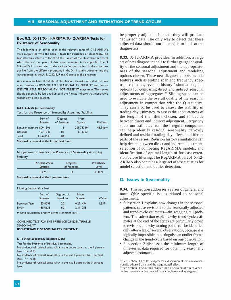
be properly adjusted. Instead, they will produce“adjusted” data. The only way to detect that theseadjusted data should not be used is to look at thediagnostics.

8.33. X-12-ARIMA provides, in addition, a largeset of new diagnostic tools to further gauge the qual-ity of the seasonal adjustment and the appropriate-ness of the seasonal adjustment and modelingoptions chosen. These new diagnostic tools includefeatures such as sliding span and frequency spec-trum estimates, revision history24 simulations, andoptions for comparing direct and indirect seasonaladjustments of aggregates.25 Sliding spans can beused to evaluate the overall quality of the seasonaladjustment in competition with the Q statistics.They can also be used to assess the stability oftrading-day estimates, to assess the adequateness ofthe length of the filters chosen, and to decidebetween direct and indirect adjustment. Frequencyspectrum estimates from the irregular componentcan help identify residual seasonality narrowlydefined and residual trading-day effects in differentparts of the series. Revision history simulations canhelp decide between direct and indirect adjustment,selection of competing RegARIMA models, andidentification of optimal length of forecast exten-sion before filtering. The RegARIMA part of X-12-ARIMA also contains a large set of test statistics formodel selection and outlier detection.

D. Issues in Seasonality

8.34. This section addresses a series of general andmore QNA-specific issues related to seasonaladjustment. • Subsection 1 explains how changes in the seasonal

patterns cause revisions to the seasonally adjustedand trend-cycle estimates—the wagging tail prob-lem. The subsection explains why trend-cycle esti-mates at the end of the series are particularly proneto revisions and why turning points can be identifiedonly after a lag of several observations, because it islogically impossible to distinguish an outlier from achange in the trend-cycle based on one observation.

• Subsection 2 discusses the minimum length oftime-series data required for obtaining seasonallyadjusted estimates.


134

24See Section D.1 of this chapter for a discussion of revisions to sea-sonally adjusted data, and the wagging tail effect.25See Section D.3.a of this chapter for a discussion of direct-versus-indirect seasonal adjustment of balancing items and aggregates.

Box 8.2. X-11/X-11-ARIMA/X-12-ARIMA Tests forExistence of Seasonality

The following is an edited copy of the relevant parts of X-12-ARIMA’smain output file with the basic F-tests for existence of seasonality. Thetest statistics values are for the full 21 years of the illustrative series, ofwhich the last four years of data were presented in Example 8.1.The D8.A and D 11 codes refer to the various “output tables” in the main out-put file from the different programs in the X-11 family, documenting thevarious steps in the A, B, C, D, E, F, and G parts of the program.

As a minimum,Table D 8.A should be checked to make sure that the pro-gram returns an IDENTIFIABLE SEASONALITY PRESENT and not anIDENTIFIABLE SEASONALITY NOT PRESENT statement. The seriesshould generally be left unadjusted if the F-tests indicate that identifiableseasonality is not present.

D8.A F-Tests for Seasonality

Test for the Presence of Seasonality Assuming Stability

Sum of Degrees Mean Squares of Freedom Square F-Value

Between quarters 809.1996 3 269.73319 43.946** Residual 497.1645 81 6.13783 Total 1306.3640 84

Seasonality present at the 0.1 percent level.

Nonparametric Test for the Presence of Seasonality AssumingStability

Kruskal-Wallis Degrees Probability Statistic of Freedom Level

53.2410 3 0.000%

Seasonality present at the 1 percent level.

Moving Seasonality Test

Sum of Degrees of MeanSquares Freedom Square F-Value

Between Years 85.8291 20 4.291454 1.857 Error 138.6635 60 2.311058

Moving seasonality present at the 5 percent level.

COMBINED TEST FOR THE PRESENCE OF IDENTIFIABLE SEASONALITYIDENTIFIABLE SEASONALITY PRESENT

D 11 Final Seasonally Adjusted Data

Test for the Presence of Residual Seasonality.No evidence of residual seasonality in the entire series at the 1 percentlevel. F = 0.03No evidence of residual seasonality in the last 3 years at the 1 percentlevel. F = 0.48No evidence of residual seasonality in the last 3 years at the 5 percentlevel.

• Subsection 3 addresses a series of issues relatedparticularly to seasonal adjustment and trend-cycle estimation of QNA data, such as preserva-tion of accounting identities, seasonal adjustmentof balancing items and aggregates, and the rela-tionship between annual data and seasonallyadjusted quarterly data.

• Finally, Subsection 4 discusses the status and pre-sentation of seasonally adjusted and trend-cycleQNA estimates.

1. Changes in Seasonal Patterns, Revisions, andthe Wagging Tail Problem

8.35. Seasonal effects may change over time. Theseasonal pattern may gradually evolve as economicbehavior, economic structures, and institutional andsocial arrangements change. The seasonal patternmay also change abruptly because of sudden institu-tional changes.

8.36. Seasonal filters estimated using centered movingaverages allow the seasonal pattern of the series tochange over time and allow for a gradual update of theseasonal pattern, as illustrated in Example 8.2. Thisresults in a more correct identification of the seasonaleffects influencing different parts of the series.

8.37. Centered moving average seasonal filters alsoimply, however, that the final seasonally adjusted val-ues depend on both past and future values of the series.Thus, to be able to seasonally adjust the earliest and lat-est observations of the series, either asymmetric filtershave to be used for the earliest and the latest observa-tions of the series or the series has to be extended by useof backcasts and forecasts based on the pattern of thetime series. While the original X-11 program usedasymmetric filters at the beginning and end of theseries, X-12-ARIMA and X-11-ARIMA use ARIMAmodeling techniques to extend the series so that lessasymmetric filters can be used at the beginning and end.

8.38. Consequently, new observations may result inchanges in the estimated seasonal pattern for the lat-est part of the series and subject seasonally adjusteddata to more frequent revisions than the original non-seasonally adjusted series. This is illustrated inExample 8.3 below. Estimates of the underlyingtrend-cycle component for the most recent parts ofthe time series in particular may be subject to rela-tively large revisions at the first updates,26 however,

theoretical and empirical studies indicate that thetrend-cycle converges much faster to its final valuethan the seasonally adjusted series. In contrast, theseasonally adjusted series may be subject to lowerrevisions at the first updates but not-negligible revi-sions even after one to two years. There are two mainreasons for slower convergence of the seasonal esti-mates. First, the seasonal moving average filters aresignificantly longer than the trend-cycle filters.27

Second, revisions to the estimated regression para-meters for calendar-related systematic effects mayaffect the complete time series. These revisions tothe seasonally adjusted and trend-cycle estimates,owing to new observations, are commonly referredto as the “wagging tail problem.”

8.39. Estimates of the underlying trend-cycle compo-nent for the most recent parts of the series should beinterpreted with care, because signals of a change in thetrend-cycle at the end of the series may be false. Thereare two main reasons why these signals may be false.First, outliers may cause significant revisions to thetrend-cycle end-point estimates. It is usually not possi-ble from a single observation to distinguish between anoutlier and a change in the underlying trend-cycle,unless a particular event from other sources generatingan outlier is known to have occurred. In general, severalobservations verifying the change in the trend-cycleindicated by the first observation are needed. Second,the moving average trend filters used at the end of theseries (asymmetric moving average filters with or with-out ARIMA extension of the series) implicitly assumethat the most recent basic trend of the series will persist.Consequently, when a turning point appears at the cur-rent end of the series, the estimated trend values at firstpresent a systematically distorted picture, continuing topoint in the direction of the former, now invalidated,trend. It is only after a lag of several observations thatthe change in the trend comes to light. While the trend-cycle component may be subject to large revisions atthe first updates, however, it typically converges rela-tively fast to its final value.28 An illustration of this canbe found by comparing the data presented in Example8.3 (seasonally adjusted estimates) with that inExample 8.4 (trend-cycle estimates).

Issues in Seasonality

135

27For instance, the seasonal factors will be final after 2 years with thedefault 5-term (3 x 3) moving average seasonal filter (as long as anyadjustments for calendar effects and outliers are not revised). In con-trast, the trend-cycle estimates will be final after 2 quarters with the5-term Henderson moving average trend-cycle filter (as long as theunderlying seasonally adjusted series is not revised).32The trend-cycle estimates will be final after 2 quarters with a 5-termHenderson moving average filter and after 3 quarters with a 7-term fil-ter as long as the underlying seasonally adjusted series is not revised.26Illustrated in Example 8.4.


136

Box 8.3. X-11-ARIMA/X-12-ARIMA M- and Q-Test Statistics

The first and third column below are from the F 3 table of X-12-ARIMA’s main output file with the M- and Q-test statistics.The test statistic values are for the full 21 years of the illustrative series, of which the last four years of data were presented in Example 8.1.The F 3 and F 2.B codes refer to the various“output tables” in the program’s main output file.

The Q-test statistic at the bottom is a weighted average of the M-test statistics.

F 3. Monitoring and Quality Assessment StatisticsAll the measures below are in the range from 0 to 3 with an acceptance region from 0 to 1.

Statistics Weight in Q Value

1. The relative contribution of the irregular component over a one-quarter span 13 M1 = 0.245 (from Table F 2.B).

2. The relative contribution of the irregular component to the stationary portion 13 M2 = 0.037of the variance (from Table F 2.F).

3. The amount of quarter-to-quarter change in the irregular component compared 10 M3 = 0.048 with the amount of quarter-to-quarter change in the trend-cycle (from Table F2.H).

4. The amount of auto-correlation in the irregular as described by the average 5 M4 = 0.875duration of run (Table F 2.D).

5. The number of quarters it takes the change in the trend-cycle to surpass the amount 11 M5 = 0.200 of change in the irregular (from Table F 2.E).

6. The amount of year-to-year change in the irregular compared with the amount 10 M6 = 0.972

of year-to-year change in the seasonal (from Table F 2.H).

7. The amount of moving seasonality present relative to the amount of stable 16 M7 = 0.378

seasonality (from Table F 2.I).

8. The size of the fluctuations in the seasonal component throughout the whole series. 7 M8 = 1.472

9. The average linear movement in the seasonal component throughout the whole series. 7 M9 = 0.240

10. Same as 8, calculated for recent years only. 4 M10= 1.935

11. Same as 9, calculated for recent years only. 4 M11= 1.935

ACCEPTED at the level 0.52 Check the three above measures that failed. Q (without M2) = 0.59 ACCEPTED.

1Based on Eurostat (1998).2Based on Statistics Canada’s seasonal adjustment course material.


137

Motivation1 Diagnose and Remedy if Fails2

The seasonal and irregular components cannot be separated sufficiently if Series too irregular.Try to preadjust the series.the irregular variation is too high compared with the variation in the seasonalcomponent. M1 and M2 test this property by using two different trend removers.

If the quarter-to-quarter movement in the irregular is too important in the SI Irregular too strong compared to trend-cycle.Try to preadjust the series.component compared with the trend-cycle, the separation of these component can be of low quality.

Test of randomness of the irregular component. (Be careful, because the estimator Irregulars are autocorrelated.Try to change length of the trend filter and of the irregular is not white noise and the statistics can be misleading.) (different) preadjustment for trading-day effects.There may be residual

trading-day effects in the series.

Similar to M3. Irregular too strong compared to trend-cycle.Try to preadjust the series.

In one step of the X-11 filtering procedure, the irregular is separated from the Irregular too strong compared with seasonality.Try to change length of

seasonal by a 3x5 seasonal moving average. Sometimes, this can be too flexible seasonal MA filter.

(I/S ratio is very high) or too restrictive (I/S ratio is very low). If M6 fails, you can

try to use the 3x1 or the stable option to adjust for this problem.

Combined F-test to measure the stable seasonality and the moving seasonality Do not seasonally adjust the series. Indicates absence of Seasonality.

in the final SI ratios. Important test statistics for indicating whether seasonality

is identifiable by the program.

Measurement of the random fluctuations in the seasonal factors.A high value Change seasonal moving average filter. Seasonality may be moving too fast.

can indicate a high distortion in the estimate of the seasonal factors.

Because one is normally interested in the recent data, these statistics give insights Look at ARIMA extrapolation. Indicate that the seasonality may be moving too

into the quality of the recent estimates of the seasonal factors.Watch these statistics fast at the end of the series

carefully if you use forecasts of the seasonal factors and not concurrent adjustment.

8.40. Studies have shown that using ARIMA modelsto extend the series before filtering generally signifi-cantly reduces the size of these revisions comparedwith using asymmetric filters.29 These studies haveshown that, typically, revisions to the level of theseries as well as to the period-to-period rate of changeare reduced. Use of RegARIMA models, as offeredby X-12-ARIMA, may make the backcasts and fore-casts more robust and thus further reduces the size ofthese revisions compared with using pure ARIMAmodels. The reason for this is that RegARIMA mod-els allow trading-day effects and other effects cap-tured by the regressors to be taken into account in theforecasts in a consistent way. Availability of longertime series should result in a more precise identifica-tion of the regular pattern of the series (the seasonalpattern and the ARIMA model) and, in general, alsoreduce the size of the revisions.

8.41. Revisions to the seasonally adjusted data can becarried out as soon as new observations become avail-able—concurrent revisions—or at longer intervals. Thelatter requires use of the one-year-ahead forecastedseasonal factors offered by X-11, X-11-ARIMA, andX-12-ARIMA to compute seasonally adjusted esti-mates for more recent periods not covered by the last

revision. Use of one-year-ahead forecast of seasonalfactors was common in the early days of seasonaladjustment with X-11 but is less common today.Besides full concurrent revisions and use of forecasts ofseasonal factors, a third alternative is to use period-to-period rates of change from estimates based on concur-rent adjustments to update previously released data andonly revise data for past periods once a year.

8.42. From a purely theoretical point of view, andexcluding the effects of outliers and revisions to theoriginal unadjusted data, concurrent adjustment isalways preferable. New data contribute new informa-tion about changes in the seasonal pattern that prefer-ably should be incorporated into the estimates as earlyas possible. Consequently, use of one-year-aheadforecasts of seasonal factors results in loss of infor-mation and, as empirical studies30 have shown and asillustrated in Example 8.5, often in larger, albeit lessfrequent, revisions to the levels as well as the period-to-period rates of change in the seasonally adjusteddata. Theoretical studies31 support this finding.

8.43. The potential gains from concurrent adjust-ment can be significant but are not always. In general


138

Example 8.2. Moving Seasonality

The chart presents the seasonal factors for the last 21 years of the time series presented in Example 8.1 and illustrates how the seasonal pattern has beenchanging gradually over time, as estimated by X-12-ARIMA.

0.90

0.94

0.98

1.02

1.06

1.10

1979 1980 1981 1982 1983 1984 1985 1986 1987 1988 1989 1990 1991 1992 1993 1994 1995 1996 1997 1998 19992000

Seasonal Factors

30See among others Dagum and Morry (1984), Hout and others.(1986), Kenny and Durbin (1982), and McKenzie (1984).31See among others Dagum (1981 and 1982) and Wallis (1982).

29See among others Bobitt and Otto (1990), Dagum (1987), Dagumand Morry (1984), Hout et al. (1986).

A-head

139


Example 8.3. Changes in Seasonal Patterns, Revisions of the Seasonally Adjusted Series, and the Wagging TailProblemRevisions to the Seasonally Adjusted Estimates by Adding New Observations(Original unadjusted data in Example 8.1.)

120

125

130

135

140

1996 1997 1998 1999 2000

Data until q1 00 Data until q4 99 Data until q3 99 Data until q2 99 Data until q1 99 Data until q4 98 Data until q3 98Period-to- Period-to- Period-to- Period-to- Period-to- Period-to- Period-to-

Period Period Period Period Period Period Period Rate of Rate of Rate of Rate of Rate of Rate of Rate of

Date Index Change Index Change Index Change Index Change Index Change Index Change Index Change

q1 1996 139.8 139.9 139.8 139.7 139.7 139.2 139.3q2 1996 134.6 –3.7% 134.6 –3.7% 134.6 –3.7% 134.5 –3.7% 134.5 –3.7% 134.4 –3.4% 134.5 –3.5%q3 1996 130.5 –3.1% 130.5 –3.1% 130.6 –3.0% 130.9 –2.7% 131.0 –2.6% 131.4 –2.2% 130.8 –2.7%q4 1996 125.7 –3.7% 125.6 –3.7% 125.6 –3.8% 125.6 –4.1% 125.6 –4.1% 125.9 –4.2% 126.3 –3.5%q1 1997 123.2 –2.0% 123.3 –1.9% 123.2 –2.0% 123.1 –2.0% 123.0 –2.0% 122.2 –2.9% 122.5 –3.0%q2 1997 127.2 3.2% 127.3 3.2% 127.2 3.3% 126.8 3.1% 126.8 3.0% 126.7 3.7% 126.8 3.5%q3 1997 130.1 2.3% 130.0 2.2% 130.3 2.4% 131.0 3.3% 131.1 3.5% 131.7 3.9% 130.7 3.1%q4 1997 129.1 –0.7% 128.9 –0.8% 128.8 –1.1% 128.7 –1.7% 128.7 –1.8% 129.3 –1.8% 130.0 –0.5%q1 1998 131.0 1.4% 131.1 1.7% 130.8 1.6% 130.7 1.6% 130.7 1.5% 129.6 0.2% 130.0 0.0%q2 1998 131.9 0.7% 132.1 0.8% 132.1 0.9% 131.4 0.5% 131.2 0.4% 131.0 1.1% 131.1 0.8%q3 1998 130.7 –1.0% 130.5 –1.2% 131.0 –0.8% 132.0 0.5% 132.2 0.7% 132.8 1.3% 131.4 0.2%q4 1998 136.4 4.4% 136.1 4.3% 136.1 3.9% 135.9 3.0% 135.9 2.8% 136.9 3.0%q1 1999 131.5 –3.6% 131.7 –3.2% 131.3 –3.5% 131.2 –3.4% 131.2 –3.5%q2 1999 131.9 0.3% 132.2 0.4% 132.1 0.6% 131.0 –0.2%q3 1999 136.5 3.4% 136.2 3.0% 136.9 3.6%q4 1999 135.5 –0.7% 135.1 –0.8%q1 2000 136.3 0.6%

Note how the seasonally adjusted data (like the trend-cycle data presented in Example 8.4 but less so) for a particular period are revised as later data become available, even when theunadjusted data for that period were not revised. In this example, adding q1 2000 results in an upward adjustment of the growth from q2 1999 to q3 1999 in the seasonally adjusted seriesfrom an estimate of 3.0 percent to a revised estimate of 3.4 percent. Minor effects on the seasonally adjusted series of adding q1 2000 can be traced all the way back to 1993.


140

Example 8.4. Changes in Seasonal Patterns, Revisions and the Wagging Tail ProblemRevisions to Trend-Cycle Estimates(Original unadjusted data in Example 8.1, seasonally adjusted in Example 8.3.)

120

125

130

135

140

1996 1997 1998 1999 2000

Data until q1 00 Data until q4 99 Data until q3 99 Data until q2 99 Data until q1 99 Data until q4 98 Data until q3 98Period-to- Period-to- Period-to- Period-to- Period-to- Period-to- Period-to-

Period Period Period Period Period Period Period Rate of Rate of Rate of Rate of Rate of Rate of Rate of

Date Index Change Index Change Index Change Index Change Index Change Index Change Index Change

q1 1996 139.8 139.9 139.8 139.7 139.7 139.2 139.3q1 1996 139.2 139.2 139.1 139.0 139.0 138.7 138.9q2 1996 135.2 –2.9% 135.2 –2.9% 135.2 –2.8% 135.2 –2.7% 135.2 –2.7% 135.0 –2.7% 135.0 –2.8%q3 1996 130.1 –3.7% 130.1 –3.8% 130.2 –3.7% 130.3 –3.6% 130.4 –3.6% 130.4 –3.4% 130.4 –3.4%q4 1996 125.7 –3.4% 125.6 –3.5% 125.6 –3.5% 125.7 –3.6% 125.7 –3.6% 126.2 –3.2% 126.6 –2.9%q1 1997 124.2 –1.2% 124.2 –1.1% 124.1 –1.2% 123.9 –1.4% 123.9 –1.4% 124.7 –1.2% 125.2 –1.1%q2 1997 126.9 2.2% 126.9 2.2% 126.8 2.1% 126.3 1.9% 126.2 1.9% 126.6 1.5% 126.7 1.2%q3 1997 129.4 2.0% 129.2 1.8% 129.1 1.8% 128.5 1.8% 128.4 1.8% 128.7 1.7% 128.8 1.7%q4 1997 129.9 0.4% 129.7 0.4% 129.5 0.4% 129.3 0.6% 129.3 0.7% 129.4 0.5% 129.9 0.8%q1 1998 130.8 0.7% 130.9 0.9% 130.7 0.9% 130.4 0.8% 130.3 0.8% 129.7 0.3% 130.3 0.4%q2 1998 131.5 0.5% 131.6 0.5% 131.6 0.7% 131.4 0.8% 131.4 0.8% 130.8 0.9% 131.0 0.5%q3 1998 131.6 0.1% 131.4 –0.2% 131.6 0.0% 132.2 0.5% 132.4 0.8% 133.3 1.9% 131.2 0.2%q4 1998 131.8 0.2% 131.6 0.2% 131.5 –0.1% 132.3 0.1% 132.7 0.3% 136.4 2.3%q1 1999 131.7 –0.1% 131.8 0.2% 131.4 –0.1% 131.5 –0.6% 131.3 –1.1%q2 1999 132.4 0.5% 132.9 0.8% 132.7 1.0% 131.1 –0.3%q3 1999 134.4 1.5% 135.1 1.6% 136.6 2.9%q4 1999 135.7 1.0% 135.0 –0.1%q1 2000 136.3 0.4%

The chart and table demonstrate how the trend-cycle estimates for a particular period may be subject to relatively large revisions as data for new periods become available, even whenthe unadjusted data for that period were not revised. In this example, adding q1 2000 results in an upward adjustment of the change in the estimated trend-cycle component from q3 1999to q4 1999, from an initial estimate of –0.1 percent to a revised estimate of 1.0 percent.

Also, observe how the strong irregular effect that occurred in q4 1998—an upward turn that disappears in the later trend-cycle estimates—wrongly resulted in an initial estimated stronggrowth from mid-1998 and onward in the earlier trend-cycle estimates.

the potential gains depend on, among other things,the following factors:• The stability of the seasonal component. A high

degree of stability in the seasonal factors implies thatthe information gain from concurrent adjustment islimited and makes it easier to forecast the seasonalfactors. On the contrary, rapidly moving seasonalityimplies that the information gain can be significant.

• The size of the irregular component. A high irregularcomponent may reduce the gain from concurrentadjustment because there is a higher likelihood forthe signals from the new observations about changesin the seasonal pattern to be false, reflecting an irreg-ular effect and not a change in the seasonal pattern.

• The size of revisions to the original unadjusteddata. Large revisions to the unadjusted data may


141

Example 8.5. Changes in Seasonal Patterns, Revisions, and the Wagging Tail ProblemConcurrent Adjustment Versus Use of One-Year-Ahead Forecast of Seasonal Factors(Original unadjusted data in Example 8.1, revisions of last seven quarters with concurrent seasonally adjusted data in Example 8.3.)

Concurrent Seasonal Period-to-Period Rate Based on Seasonal Factors Period-to-Period RateDate Adjustment of Change Forecast from q1 1999 of Change

q1 1996 139.8 139.7q2 1996 134.6 –3.7% 134.5 –3.7%q3 1996 130.5 –3.1% 131.0 –2.6%q4 1997 125.7 –3.7% 125.6 –4.1%q1 1997 123.2 –2.0% 123.0 –2.0%q2 1997 127.2 3.2% 126.8 3.0%q3 1997 130.1 2.3% 131.1 3.5%q4 1997 129.1 –0.7% 128.7 –1.8%q1 1998 131.0 1.4% 130.7 1.5%q2 1998 131.9 0.7% 131.2 0.4%q3 1998 130.7 –1.0% 132.2 0.7%q4 1998 136.4 4.4% 135.9 2.8%q1 1999 131.5 –3.6% 131.2 –3.5%q2 1999 131.9 0.3% 130.8 –0.3%q3 1999 136.5 3.4% 138.6 6.0%q4 1999 135.5 –0.7% 134.9 –2.7%q1 2000 136.3 0.6% 136.0 0.8%

The chart and table demonstrate the effect of current update (concurrent adjustment) versus use of one-year-ahead forecast seasonal factors.As can be seenby comparing with Example 8.3, use of one-year-ahead forecasts of the seasonal factors results in loss of information and larger, but less frequent, revisions. Inparticular, in this example, using one-year-ahead forecasts of the seasonal factors gave an initial estimated decline from q3 to q4 1999 in the seasonally adjust-ed series of –2.7 percent, which is substantially larger compared with the initial estimate of –0.8 percent with current update of the seasonal factors (seeExample 8.3).

120

125

130

135

140

1996 1997 1998 1999 2000

Concurrent Seasonal Adjustment

Based on Seasonal Factors Forecast from q1 1999

reduce the gain from concurrent adjustmentbecause there is a higher likelihood for the sig-nals from the new observations about changes inthe seasonal pattern to be false.

2. Minimum Length of the Time Series forSeasonal Adjustment

8.44. Five years of data and relatively stable seasonal-ity are required in general as a minimum length toobtain properly seasonally adjusted estimates. Forseries that show particularly strong and stable seasonalmovements, it may be possible to obtain seasonallyadjusted estimates based on only three years of data.

8.45. A longer time series, however, is required toidentify more precisely the seasonal pattern and toadjust the series for calendar variations (i.e., trad-ing days and moving holidays), breaks in the series,outliers, and particular events that may haveaffected the series and may cause difficulties inproperly identifying the seasonal pattern of theseries.

8.46. For countries that are setting up a new QNA sys-tem, at least five years of retrospective calculations arerecommended to conduct seasonal adjustment.

8.47. If a country has gone through severe structuralchanges resulting in radical changes in the seasonalpatterns, it may not be possible to seasonally adjustits data until several years after the break in the series.In such cases, it may be necessary to seasonallyadjust the pre-break and post-break part of the seriesseparately.

3. Critical Issues in Seasonal Adjustment of QNA

8.48. When producing seasonally adjusted nationalaccount estimates, four critical issues must be decided:(a) Should balancing items and aggregates be sea-

sonally adjusted directly or derived residually,and should accounting and aggregation relation-ships be maintained?

(b) Should the relationship among current pricevalue, price indices, and volume estimates bemaintained, and, if so, which component shouldbe derived residually?

(c) Should supply and use and other accounting iden-tities be maintained, and, if so, what are the prac-tical implications?

(d) Should the relationship to the annual accounts bestrictly preserved?

a. Compilation levels and seasonal adjustment ofbalancing items and aggregates

8.49. Seasonally adjusted estimates for balancingitems and aggregates can be derived directly or indi-rectly from seasonally adjusted estimates for the dif-ferent components; generally the results will differ,sometimes significantly. For instance, a seasonallyadjusted estimate for value added in manufacturing atcurrent prices can be derived either by seasonallyadjusting value added directly or as the differencebetween seasonally adjusted estimates for output andintermediate consumption at current prices.Similarly, a seasonally adjusted estimate for GDP atcurrent prices can be derived either by seasonallyadjusting GDP directly or as the sum of seasonallyadjusted estimates for value added by activity (plustaxes on products). Alternatively, a seasonallyadjusted estimate for GDP can be derived as the sumof seasonally adjusted estimates for the expenditurecomponents.

8.50. Conceptually, neither the direct approach northe indirect approach is optimal. There are argumentsin favor of both approaches. It is convenient, and forsome uses crucial, that accounting and aggregationrelationships are preserved.32 Studies33 and practice,however, have shown that the quality of the seasonallyadjusted series, and especially estimates of the trend-cycle component, may be improved, sometimes sig-nificantly, by seasonally adjusting aggregates directlyor at least at a more aggregated level. Practice hasshown that seasonally adjusting the data at a detailedlevel can leave residual seasonality in the aggregates,may result in less smooth seasonally adjusted series,and may result in series more subject to revisions.Which compilation level for seasonal adjustment givesthe best results varies from case to case and depends onthe properties of the particular series.

8.51. For aggregates, the direct approach may givethe best results if the component series shows thesame seasonal pattern or if the trend-cycles of theseries are highly correlated. If the component seriesshows the same seasonal pattern, aggregation oftenreduces the impact of the irregular components of thecomponent series, which at the most detailed level(the level of the source data) may be too dominant for


142

32However, for time series of chain-linked price indices and volumedata, these accounting relationships are already broken (see SectionD.4 of Chapter IX for a discussion of the non-additivity feature ofchain-linked measures).33See, among others, Dagum and Morry (1984).

proper seasonal adjustment. This effect may be par-ticularly important for small countries where irregu-lar events have a stronger impact on the data.Similarly, if the component series do not show thesame seasonal pattern but their trend-cycles arehighly correlated, aggregation reduces the impact ofboth the seasonal and irregular components of thecomponent series.

8.52. In other cases, the indirect approach may givethe best results. For instance, if the component seriesshow very different seasonal patterns and the trend-cycles of the series are uncorrelated, aggregation mayincrease the appearance of irregular movements in theaggregate. Similarly, aggregation may cause large,highly volatile nonseasonal component series to over-shadow seasonal component series, making it difficultor impossible to identify any seasonality that is presentin the aggregate series. Moreover, it may be easier toidentify breaks, outliers, calendar effects, the seasonaleffect narrowly defined, and so on in detailed serieswith low to moderate irregular components thandirectly from the aggregates, because at the detailedlevel these effects may display a simpler pattern.

8.53. For balancing items, there is reason to believethat the indirect approach more often gives betterresults. Because balancing items are derived as thedifference between two groups of component series,in the balancing item, the impact of the irregularcomponents of the component series is more likely tobe compounded. In contrast, because aggregates arederived by summation, opposite irregular movementsin the component series will cancel each other out.

8.54. Some seasonal adjustment programs,including the X-11-ARIMA and the X-12-ARIMA, offer the possibility of adjusting aggre-gates using the direct and indirect approachsimultaneously and comparing the results. Forinstance, the X-12-ARIMA, using the Compositeseries specifications command, adjusts aggregatessimultaneously using the direct and indirectapproach and provides users with a set of test sta-tistics to compare the results. These test statisticsare primarily the M and Q statistics presented inExample 8.4, measures of smoothness, and fre-quency spectrum estimates from the directly andindirectly estimated irregular component. In addi-tion, sliding span and revision history simulationtests for both the direct and the indirect estimatesare available to assess which approach results inestimates less subject to revisions.

8.55. In practice, the choice between direct and indi-rect seasonal adjustment should be based on the mainintended use of the estimates and the relativesmoothness and stability of the derived estimates. Forsome uses, preserved accounting and aggregationrelationships in the data may be crucial, and thesmoothness and stability of the derived estimates sec-ondary. For other uses, the time-series properties ofthe derived estimates may be crucial, while account-ing and aggregation relationships may be of noimportance. If the difference is insignificant, repre-senting a minor annoyance rather than adding anyuseful information, most compilers will opt for pre-serving accounting and aggregation relationshipsbetween published data.

8.56. Consequently, international practice varieswith respect to the choice between direct and indirectseasonal adjustment. Many countries obtain the sea-sonally adjusted QNA aggregates as the sum ofadjusted components, while some also adjust thetotals independently, with discrepancies between theseasonally adjusted total and the sum of the compo-nent series as a result. Finally, some countries onlypublish seasonally adjusted estimates for main aggre-gates and typically seasonally adjust these directly orderive them indirectly by adjusting rather aggregatedcomponent series.

b. Seasonal adjustment and the relationship amongprice, volume, and value

8.57. As for balancing items and aggregates, season-ally adjusted estimates for national accounts priceindices, volume measures, and current price data canbe derived either by seasonally adjusting the threeseries independently or by seasonally adjusting twoof them and deriving the third as a residual, if all threeshow seasonal variations.34 Again, because of nonlin-earities in the seasonal adjustment procedures, thealternative methods will give different results; how-ever, the differences may be minor. Preserving therelationship among the price indices, volume mea-sures, and the current price data is convenient forusers.35 Thus, it seems reasonable to seasonallyadjust two of them and derive a seasonally adjustedestimate for the third residually. Choosing whichseries to derive residually must be determined on acase-by-case basis, depending on which alternativeseems to produce the most reasonable result.

A-head

143


34Experience has shown that the price data may not always show iden-tifiable seasonal variations.35Note that chain-linking preserves this relationship (V = P • Q).

c. Seasonal adjustment and supply and use and otheraccounting identities

8.58. Seasonal adjustment may cause additionalstatistical discrepancies in seasonally adjusted databetween supply and use, GDP estimated from alter-native sides, and between the different sides ofother accounting identities. These statistical dis-crepancies are caused by nonlinearities in the sea-sonal filters, as well as use of different filter length,use of different pre-adjustments, and differences inestimated calendar effects on the various sides ofthe accounting identity. The statistical discrepan-cies may be reduced by forcing the programs tochoose the same filter length and use the same pre-adjustment factors and calendar-effect factors forall series. This may, however, reduce the smooth-ness and stability of the individual seasonallyadjusted series.

d. Seasonal adjustment and consistency with annualaccounts8.59. Annual totals based on the seasonallyadjusted data will not automatically—and oftenshould not conceptually—be equal to the corre-sponding annual totals based on the original unad-justed data. The number of working days, theimpact of moving holidays, and other calendar-related effects vary from year to year. Similarly,moving seasonality implies that the impact of theseasonal effect narrowly defined will vary fromyear to year. Thus, conceptually, for series withsignificant calendar-related effects or moving sea-sonality effects, the annual totals of a seasonallyadjusted series should differ from the unadjustedseries.

8.60. For series without any significant calendar-related or moving seasonality effects, X-11/X-12will produce seasonally adjusted data that automat-ically add up to the corresponding unadjustedannual totals if the seasonal components are addi-tive (equation 8.1) but not if the seasonals are mul-tiplicative (equation 8.2). Multiplicative seasonalfactors require that a current-period weighted aver-age of the seasonal factors averages to 1 and for theseasonally adjusted data to automatically add up tothe corresponding unadjusted annual totals.However, the normalization of the seasonal factorsin step (d) of the filtering procedure in stages 1 and2 described in paragraph 8.23 only ensures that theunweighted, and not the weighted, annual averageof the seasonal factors averages 1. It follows that,

for series with multiplicative seasonal factors andno significant calendar-related or moving seasonal-ity effects, the difference between the annual totalsof the adjusted and unadjusted series will depend onthe amplitude of the seasonal variation narrowlydefined, the volatility of the seasonally adjustedseries, and the pace of the change in the underlyingtrend-cycle. The difference will be small, and ofteninsignificant, for series with moderate to low sea-sonal amplitudes and for series with little volatilityand trend-cycle change.

8.61. X-11-ARIMA and X-12-ARIMA provideoptions for forcing the annual totals from the season-ally adjusted data to be equal to the original totals.Seasonal adjustment experts, however, generallyrecommend not using the forcing option36 if theseries show significant37 trading-day, other calendar-related, or moving seasonality effects and trading-day or other calendar adjustments are performed. Insuch cases, consistency with the annual series wouldbe achieved at the expense of the quality of the sea-sonal adjustment and would be conceptually wrong.

4. Status and Presentation of Seasonally Adjustedand Trend-Cycle QNA Estimates

8.62. The status and presentation of seasonallyadjusted and trend-cycle QNA estimates vary. Somecountries publish seasonally adjusted estimates foronly a few main aggregates and present them as addi-tional (sometimes unofficial) analytical elaborationsof the official data. Other countries focus on the sea-sonally adjusted and trend-cycle estimates and pub-lish an almost complete set of seasonally adjustedand trend-cycle QNA estimates in a reconciledaccounting format. They may present the originalunadjusted data as supplementary information.

8.63. The mode of presentation also varies substan-tially. Seasonally adjusted and trend-cycle data can bepresented as charts; as tables with the actual data,either in money values or as index series; and as tableswith derived measures of quarter-to-quarter rates ofchange. The last may be presented as the actual rates ofchange or as annualized rates (see Box 8.4).


144

36The X-12-ARIMA manual explicitly recommends against using theforcing option if trading-day adjustment is performed or if the sea-sonal pattern is changing rapidly.37Relative to the “adding-up error” introduced by the unweighted, andnot the weighted, annual average of the seasonal factors averaging to1 for multiplicative seasonal adjustment.

8.64. The rates of change are sometimes annualized tomake it easier for the layman to interpret the data. Mostusers have a feel for the size of annual growth rates butnot for monthly or quarterly rates. Annualizing growthrates, however, also means that the irregular effects arecompounded. Irrespectively of whether the actual orannualized quarterly rates of change are presented, it isimportant to indicate clearly what the data represent.

8.65. Growth rates representing different measuresof change can easily be confused unless it is clearlyindicated what the data represent. For instance, termslike “annual percentage change” or “annual rate ofgrowth” can mean (a) the rate of change from onequarter to the next annualized (at annual rate); (b) thechange from the same period of the previous year; (c)the change from one year to the next in annual data,or, equivalently, the change from the average of oneyear to the average of the next year; or (d) the changefrom the end of one year to the end of the next year.

8.66. Some countries also present the level of quar-terly current and constant price data at annualizedlevels by multiplying the actual data by four. Thisseems artificial, does not make the data easier tointerpret, and may be confusing because annual flowdata in monetary terms no longer can be derived asthe sum of the quarters. Users not familiar with thepractice of annualizing levels of current and constantprice data by multiplying the actual data by four mayconfuse annualized levels with forecast annual data.For these reasons, this practice is not recommended.

8.67. Finally, whether to present seasonallyadjusted data or estimates of the trend-cycle com-ponent is still the subject of debate between expertsin this area. In this manual, it is recommended topresent both, preferably in the form of graphsincorporated into the same chart, as illustrated inExample 8.6.

8.68. An integrated graphical presentation high-lights the overall development in the two seriesover time, including the uncertainties representedby the irregular component. In contrast, measuresof quarter-to-quarter rates of change (in particular,annualized rates) may result in an overemphasis onthe short-term movements in the latest and mostuncertain observations at the expense of the generaltrend in the series. The underlying data and derivedmeasures of quarter-to-quarter rates of change,however, should be provided as supplementaryinformation.

8.69. The presentation should highlight the lower reli-ability, particularly for the trend-cycle component, ofthe estimates for the latest observations as discussed inthis section. Means of highlighting the lower quality ofthe end-point estimates include (a) noting past revi-sions to these estimates; (b) suppressing estimates ofthe trend-cycle component for the latest observationsin graphical presentations, as in Example 8.6; and (c)showing estimates for the latest observations with atrumpet on graphical presentations and with an esti-mated confidence interval in tabular presentations.

A-head

145



146

Example 8.6. Presentation of Seasonally Adjusted Series and the Corresponding Trend-Cycle Component (Based on data from Example 8.1.)

Presenting the seasonally adjusted series and estimates of the trend-cycle components in the same chart highlights the overall development in the two seriesover time, including the uncertainties represented by the irregular component. Suppressing in the chart the estimates of the trend-cycle component at the endof the series or showing the trend-cycle estimates at the end with a trumpet based on estimated confidence intervals further highlights the added uncertain-ties at the end of the series.

120

125

130

135

140

1996 1997 1998 1999

Seasonally adjusted series

Trend-cycle component

Box 8.4. Annualizing, or Compounding, Growth Rates

Period-to-period rates of change in quarterly data can be annualized using the following compounding formula:arq,y = (1 + rq,y)

4 – 1, rq,y = (Xq,y /Xq–1,y – 1)where:arq,y Annualized quarter-to-quarter rate of change for quarter q of year y.rq,y Original quarter-to-quarter rate of change for quarter q of year y in time series Xq ,y .

The purpose of annualizing the rates of change is to present period-to-period rates of change for different period lengths on the same scaleand thus to make it easier for the layman to interpret the data. For instance, annualizing the rates of change may help to clarify that a 0.8 per-cent growth from one month to the next is equivalent to:

• 2.4 percent growth from one quarter to the next (2.4% = [(1 + 0.008)3 – 1] • 100), or • 10.0 percent growth from one year to the next (10.0% = [(1 + 0.024)4 – 1] • 100 =[(1 + 0.008)12 – 1] • 100).Most users have a feel for annual growth rates and immediately recognize that a 10.0 percent annual growth in, for example, constant pricehousehold consumption expenditures is a lot, while 0.8 percent from one month to the next appears meager.

Annualized quarterly growth rates do not indicate what the annual growth will be and are not intended to be simple forecasts of what theannual growth rate would be if this growth continues for four quarters.The quarterly growth rate has to be constant for eight quarters forthe annualized quarterly growth rate to be equal to the annual growth rate.

VIII Seasonal Adjustment and Estimation of Trend-Cycles · PDF fileVIII Seasonal Adjustment...

Documents

Transcript of VIII Seasonal Adjustment and Estimation of Trend-Cycles · PDF fileVIII Seasonal Adjustment...