Cooperative Research Program

TTI: 0-6927

Technical Report 0-6927-P6

Guide for Seasonal Adjustment and Crowdsourced Data Scaling

in cooperation with the Federal Highway Administration and the

Texas Department of Transportation http://tti.tamu.edu/documents/0-6927-P6.pdf

TEXAS A&M TRANSPORTATION INSTITUTE

COLLEGE STATION, TEXAS

Technical Report Documentation Page 1. Report No. FHWA/TX-18/0-6927-P6

2. Government Accession No. 3. Recipient's Catalog No.

4. Title and SubtitleGUIDE FOR SEASONAL ADJUSTMENT AND CROWDSOURCED DATA SCALING

5. Report Date Published: December 2018 6. Performing Organization Code

7. Author(s) Bahar Dadashova, Greg Griffin, Subasish Das, Shawn Turner, and Madison Graham

8. Performing Organization Report No.Product 0-6927-P6

9. Performing Organization Name and Address Texas A&M Transportation Institute The Texas A&M University System College Station, Texas 77843-3135

10. Work Unit No. (TRAIS)

11. Contract or Grant No. Project 0-6927

12. Sponsoring Agency Name and Address Texas Department of Transportation Research and Technology Implementation Office 125 E. 11th Street Austin, Texas 78701-2483

13. Type of Report and Period Covered Product February 2018–August 2018 14. Sponsoring Agency Code

15. Supplementary NotesProject performed in cooperation with the Texas Department of Transportation and the Federal Highway Administration. Project Title: Evaluation of Bicycle and Pedestrian Monitoring Equipment to Establish Collection Database and Methodologies for Estimating Non-Motorized Transportation URL: http://tti.tamu.edu/documents/0-6927-P6.pdf 16. Abstract

This guide describes two different adjustment processes that can be used with pedestrian and bicyclist data. The first adjustment process is seasonal adjustment, which is applied to short-duration counts that are collected during a specific month of the year. Seasonal adjustment annualizes the short-duration counts, such that the resulting adjusted count value is a better estimate of the annual average daily traffic. This guide provides monthly adjustment factors for both pedestrian and bicyclist count data, which is recommended for use with all short-duration count data that include at least seven days of data.

The second adjustment process described in this guide is crowdsourced data scaling, which is applied to crowdsourced bicyclist data samples that are collected from GPS-enabled smartphones. Because the crowdsourced data represent only a sample of the total bicyclists, the number of samples must be scaled or expanded to estimate the total number of bicyclists. This guide describes a simple scaling process that estimates average annual daily bicyclists using the number of crowdsourced data samples, the functional class of the bicyclist travel facility, and the density of high-income households near the bicyclist travel facility.

17. Key WordsPedestrian and Bicyclist Count Data, Seasonal Adjustment Factors, Crowdsourced Data Scaling

18. Distribution Statement No restrictions. This document is available to the public through NTIS: National Technical Information Service Alexandria, Virginia http://www.ntis.gov

19. Security Classif. (of this report) Unclassified

20. Security Classif. (of this page) Unclassified

21. No. of Pages 76

22. Price

Form DOT F 1700.7 (8-72) Reproduction of completed page authorized

GUIDE FOR SEASONAL ADJUSTMENT AND CROWDSOURCED DATA SCALING

by

Bahar Dadashova Associate Transportation Researcher Texas A&M Transportation Institute

Greg Griffin Assistant Research Scientist

Texas A&M Transportation Institute

Subasish Das Associate Transportation Researcher Texas A&M Transportation Institute

Shawn Turner Senior Research Engineer

Texas A&M Transportation Institute

and

Madison Graham Graduate Research Assistant

Texas A&M Transportation Institute

Product 0-6927-P6 Project 0-6927

Project Title: Evaluation of Bicycle and Pedestrian Monitoring Equipment to Establish Collection Database and Methodologies for Estimating Non-Motorized Transportation

Performed in cooperation with the Texas Department of Transportation

and the Federal Highway Administration

Published: December 2018

TEXAS A&M TRANSPORTATION INSTITUTE College Station, Texas 77843-3135

v

DISCLAIMER This research was performed in cooperation with the Texas Department of Transportation (TxDOT) and the Federal Highway Administration (FHWA). The contents of this report reflect the views of the authors, who are responsible for the facts and the accuracy of the data presented herein. The contents do not necessarily reflect the official view or policies of the FHWA or TxDOT. This report does not constitute a standard, specification, or regulation.

The United States Government and the State of Texas do not endorse products or manufacturers. Trade or manufacturers’ names appear herein solely because they are considered essential to the object of this report.

vi

ACKNOWLEDGMENTS This project was conducted in cooperation with TxDOT and FHWA. The authors thank the following members of the project monitoring committee:

• Project Manager: Chris Glancy, TxDOT. • Lead: Teri Kaplan, TxDOT. • Co-Lead: Bonnie Sherman, TxDOT. • Mark Wooldridge, TxDOT. • Bill Knowles, TxDOT. • Greg Goldman, TxDOT. • Darren McDaniel, TxDOT. • Adam Chodkiewicz, TxDOT. • Shelly Harris, TxDOT. • Benjamin Miller, TxDOT. • Michael Flaming, TxDOT. • Ana Ramirez Huerta, TxDOT. • Mahendran Thivakaran, TxDOT. • Diane Dohm, Houston-Galveston Area Council. • Kelly Porter, Capital Area Metropolitan Planning Organization. • Karla Weaver, North Central Texas Council of Governments. • Alexandria Carroll, Alamo Area Metropolitan Planning Organization. • Jeffrey Pollack, Corpus Christi Metropolitan Planning Organization. • Francis Reilly, City of Austin. • Anita Holman, City of Houston. • Carl Seifert, Jacobs Engineering.

vii

TABLE OF CONTENTS

Page List of Figures .............................................................................................................................. viii List of Tables ................................................................................................................................. ix Chapter 1. Introduction ................................................................................................................... 1

Seasonal Adjustment ................................................................................................................... 1 Crowdsourced Data Scaling ........................................................................................................ 1

Chapter 2. Seasonal Adjustment Factors ........................................................................................ 3 Chapter 3. Crowdsourced Data Scaling .......................................................................................... 7

Introduction ................................................................................................................................. 7 Overview: Developing Factors to Scale Crowdsourced Bicycle Volumes ................................. 7 Steps to Estimate Bicycle Traffic with Crowdsourced Data ....................................................... 8 Summary and Caveats of Using AADB Estimation Models .................................................... 11

References ..................................................................................................................................... 13 Appendix A. Pedestrian and Bicyclist Traffic Patterns at Permanent Counter Locations in

Texas ................................................................................................................................. 15 Appendix B. Development of Procedures for Crowdsourced Data Scaling ................................. 49

Selection of Most Influential Variables .................................................................................... 49 Model Estimation Results ......................................................................................................... 54 Prediction Error Measures ......................................................................................................... 58

viii

LIST OF FIGURES

Figure 1. Chart Illustrating Similar Seasonal Patterns for Different Factor Groups. ..................... 4 Figure 2. Month-of-Year Count Adjustment Factors for Short-Duration Counts. ......................... 5 Figure 3. Bicyclist Traffic Patterns: Johnson Creek Trail @ MoPac/W 5th St./W 6th St.

Interchange (Austin). ........................................................................................................ 15 Figure 4. Pedestrian Traffic Patterns: Johnson Creek Trail @ MoPac/W 5th St./W 6th St.

Interchange (Austin). ........................................................................................................ 16 Figure 5. Bicyclist Traffic Patterns: Lance Armstrong Bikeway @ Waller Creek (Austin). ....... 17 Figure 6. Pedestrian Traffic Patterns: Lance Armstrong Bikeway @ Waller Creek (Austin)...... 18 Figure 7. Bicyclist Traffic Patterns: Manor Rd. @ Alamo St. (Austin). ...................................... 19 Figure 8. Bicyclist Traffic Patterns: Walnut Creek Trail N of Jain Ln. (Austin). ........................ 20 Figure 9. Pedestrian Traffic Patterns: Walnut Creek Trail N. of Jain Ln. (Austin). ..................... 21 Figure 10. Bicyclist Traffic Patterns: Heights Trail @ 5 ½ Street (Houston). ............................. 22 Figure 11. Pedestrian Traffic Patterns: Heights Trail @ 5 ½ Street (Houston). ........................... 23 Figure 12. Bicyclist Traffic Patterns: Bluebonnet Trail at US 75 (Plano). ................................... 24 Figure 13. Pedestrian Traffic Patterns: Bluebonnet Trail at US 75 (Plano). ................................ 25 Figure 14. Bicyclist Traffic Patterns: OPP and NP Trail (Plano). ................................................ 26 Figure 15. Pedestrian Traffic Patterns: OPP and NP Trail (Plano). .............................................. 27 Figure 16. Bicyclist Traffic Patterns: Legacy Trail (Plano). ........................................................ 28 Figure 17. Pedestrian Traffic Patterns: Legacy Trail (Plano). ...................................................... 29 Figure 18. Bicyclist Traffic Patterns: Mission Reach Trail South of Theo Ave. (San

Antonio). ........................................................................................................................... 30 Figure 19. Pedestrian Traffic Patterns: Mission Reach Trail South of Theo Ave. (San

Antonio). ........................................................................................................................... 31 Figure 20. Bicyclist Traffic Patterns: Bachman Lake/W North West Highway (Dallas). ............ 32 Figure 21. Pedestrian Traffic Patterns: Bachman Lake/W North West Highway (Dallas). ......... 33 Figure 22. Bicyclist Traffic Patterns: Katy Trail at Cedar Springs Rd. (Dallas). ......................... 34 Figure 23. Pedestrian Traffic Patterns: Katy Trail at Cedar Springs Rd. (Dallas). ....................... 35 Figure 24. Bicyclist Traffic Patterns: Katy Trail at Fitzhugh (Dallas). ........................................ 36 Figure 25. Pedestrian Traffic Patterns: Katy Trail at Fitzhugh (Dallas). ...................................... 37 Figure 26. Bicyclist Traffic Patterns: Katy Trail at Harvard Avenue (Dallas). ............................ 38 Figure 27. Pedestrian Traffic Patterns: Katy Trail at Harvard Avenue (Dallas). ......................... 39 Figure 28. Bicyclist Traffic Patterns: Katy Trail (Houston Street/AA Center) (Dallas). ............. 40 Figure 29. Pedestrian Traffic Patterns: Katy Trail (Houston Street/AA Center) (Dallas). ........... 41 Figure 30. Bicyclist Traffic Patterns: White Rock Trail at Big Thicket (Dallas). ........................ 42 Figure 31. Pedestrian Traffic Patterns: White Rock Trail at Big Thicket (Dallas). ...................... 43 Figure 32. Bicyclist Traffic Patterns: White Rock Lake Trail (at Fisher) (Dallas). ..................... 44 Figure 33. Pedestrian Traffic Patterns: White Rock Lake Trail (at Fisher) (Dallas). ................... 45 Figure 34. Bicyclist Traffic Patterns: White Rock Lake Trail at Winfrey Point (Dallas). ........... 46 Figure 35. Pedestrian Traffic Count Patterns: White Rock Lake Trail at Winfrey Point

(Dallas). ............................................................................................................................. 47 Figure 36. Initial List of Important Variables. .............................................................................. 51 Figure 37. Final List of Important Variables. ............................................................................... 52 Figure 38. Prediction Intervals. ..................................................................................................... 58

ix

LIST OF TABLES

Table 1. Estimated Annual Bicycle Traffic Given Strava Activity and Roadway Class. ............. 11 Table 2. List of Variables Considered for the Analysis. ............................................................... 49 Table 3. Descriptive Statistics of Strava Sample Percentages. ..................................................... 50 Table 4. Number of Locations per Percentile Groups. ................................................................. 50 Table 5. CLAZZ Definitions......................................................................................................... 53 Table 6. Estimation Results, Model 1. .......................................................................................... 56 Table 7. Estimation Results, Model 2. .......................................................................................... 57 Table 8. Relative Accuracy per Strava Percentage Categories. .................................................... 59 Table 9. Prediction Error per Strava Percentile Groups. .............................................................. 59 Table 10. Prediction Intervals. ...................................................................................................... 60

1

CHAPTER 1. INTRODUCTION

This guide describes two different adjustment processes that can be used with pedestrian and bicyclist data:

• Seasonal adjustment. • Crowdsourced data scaling.

Both adjustment processes and their purpose are introduced in the following paragraphs.

SEASONAL ADJUSTMENT

The first adjustment process is seasonal adjustment, which is applied to short-duration counts that are collected during a specific month of the year. Seasonal adjustment annualizes the short-duration counts, such that the resulting adjusted count value is a better estimate of the annual average daily traffic (AADT). A similar adjustment process is also used for short-duration motor vehicle counts that are collected on specific days and specific months.

Chapter 2 in this guide provides monthly adjustment factors for both pedestrian and bicyclist count data, which is recommended for use with all short-duration count data that include at least seven days of data. The monthly adjustment factors are based on continuous count data collected from 17 different permanent counter locations in Austin, Dallas, Houston, Plano, and San Antonio. Appendix A includes numerous charts that illustrate the month-of-year, time-of-day, and day-of-week traffic patterns at these permanent counter locations.

CROWDSOURCED DATA SCALING

The second adjustment process described in Chapter 3 is crowdsourced data scaling, which is applied to crowdsourced bicyclist data samples that are collected from GPS-enabled smartphones. Because the crowdsourced data represent only a sample of the total bicyclists, the number of samples must be scaled or expanded to estimate the total number of bicyclists.

Researchers developed the crowdsourced data scaling process by comparing crowdsourced data samples to actual ground counts at 100 locations throughout Texas. The sample rates varied considerably among the locations, and explanatory variables were tested to determine what variables had the strongest influence on the crowdsourced data sample rate. Researchers then developed simplified equations that included the most influential variables.

Chapter 3 describes the resulting crowdsourced data scaling process that estimates average annual daily bicyclists (AADB) using the number of crowdsourced data samples, the functional class of the bicyclist travel facility, and the density of high-income households near the bicyclist travel facility.

3

CHAPTER 2. SEASONAL ADJUSTMENT FACTORS

Seasonal adjustment factors are used to process short-duration traffic counts to more accurately estimate AADT, one of the most common traffic count statistics. For example, if bicyclist counts are collected during a month when fewer bicyclists are riding, the collected bicyclist counts should be adjusted up to better represent annual average bicycling levels. Similarly, if pedestrian counts are collected during a month when more people are walking, these collected pedestrian counts should be adjusted down to better represent annual average walking levels. Traffic count analysts routinely use seasonal adjustment factors to annualize motor vehicle counts, as recommended in the Federal Highway Administration’s Traffic Monitoring Guide (TMG) (FHWA 2016).

Researchers developed pedestrian and bicyclist seasonal adjustment factors using the methods outlined in the 2016 edition of the TMG. For non-motorized traffic, these methods are detailed in pages 4-25 through 4-32 (Section 4.4). The factor development methods for non-motorized traffic are very similar to those for motorized traffic detailed on pages 3-16 through 3-30 (Section 3.2.1). In general, the method is outlined as follows:

1. Create a summary of traffic count patterns from continuous counters: Develop month-of-year, day-of-week, and time-of-day summary charts.

2. Identify distinct traffic patterns: Examine charts to identify which continuous counters are most similar or dissimilar.

3. Classify continuous counters into unique factor groups: Combine continuous counter locations into unique factor groups.

4. Calculate average adjustment factors from each factor group: Calculate average adjustment factors that can be applied to short-duration counts.

In Step 1, researchers created numerous charts to display pedestrian and bicyclist count patterns separately by time-of-day, day-of-week, and month-of-year (see Appendix A). These charts were created for all 17 permanent counters that had at least one full calendar year of complete and valid count data.

In Steps 2 and 3, researchers examined the pedestrian and bicyclist count patterns for each available count location, and classified each location into one of these factor groups as listed in the 2016 TMG:

• Commuter and work/school-based trips: typically have the highest peaks in the morning and evening.

• Recreation/utilitarian: may peak only once daily or be evenly distributed throughout the day.

• Mixed trip purposes (both commuter and recreation/utilitarian): have varying levels of these two different trip purposes, or may include other miscellaneous trip purposes.

4

TTI’s preliminary analysis identified the following number of permanent counter locations in each factor group:

• Commuter and work/school-based trips: one location for pedestrians, one different location for bicyclists.

• Recreation/utilitarian: five locations for pedestrians, two locations for bicyclists. • Mixed trip purposes: 11 locations for pedestrians, 10 locations for bicyclists.

Since the statewide pedestrian and bicyclist count database currently includes only short-duration counts of at least seven days (including at least one day of each day of the week), the seasonal adjustment would only need to account for the month of year and not the day of week. Therefore, researchers further analyzed the preliminary factor groups by examining the month-of-year patterns. In looking at these seasonal patterns, researchers concluded that the month-of-year patterns were quite similar, even among different factor groups (Figure 1). To simplify the seasonal adjustment process, TTI combined all analyzed permanent count locations in the three factor groups to create month-of-year count adjustment factors (Figure 2).

Figure 1. Chart Illustrating Similar Seasonal Patterns for Different Factor Groups.

5

Figure 2. Month-of-Year Count Adjustment Factors for Short-Duration Counts.

To apply these adjustment factors, the seven-day average daily traffic (ADT) volume is multiplied by the factor corresponding to the travel mode and month of short-duration counts. For example, if a seven-day ADT in July for pedestrians is 100 persons, then the annualized ADT (or AADT) is 100×107 percent, or 107 pedestrians. Similarly, if a seven-day ADT in April for bicyclists is 50, then the AADT is 50×86 percent, or 43 bicyclists.

7

CHAPTER 3. CROWDSOURCED DATA SCALING

INTRODUCTION

Traffic volumes are fundamental for evaluating transportation systems, regardless of travel mode. A lack of counts for non-motorized modes poses a challenge for practitioners developing and managing multimodal transportation facilities, whether they want to evaluate transportation safety, potential need for infrastructure changes, or to answer other questions about how and where people bicycle and walk. This chapter shows how to take advantage of new data sources that provide a limited and biased sample of trips, then combine them with traditional counts to estimate bicycle travel volumes across most of the state of Texas.

Crowdsourcing uses a broad pool of individuals through an online platform that aggregates and formats the information for a specific use. In this case, bicyclist travel is crowdsourced through a smartphone-based app called Strava, used by bicyclists who want to record and compare their trips. The company aggregates these trips onto a transportation system network, processes them for privacy, and then re-sells the information as a crowdsourced traffic data product, available in many places around the globe. However, only a small portion of all bicyclists use the app, and this proportion varies across time and space. For instance, researchers found 3–9 percent of bicycle trips counted on trails in Austin used Strava at the time of the count (Griffin and Jiao 2015a), but this proportion varies in different contexts and over time (Jestico et al. 2016; Conrow et al. 2018).

Researchers developed a method to scale crowdsourced bicycle trips by using limited on-ground count data and other factors, resulting in a relatively simple process to estimate bicycle travel using crowdsourced data, combined with the functional class of a network segment from Open Street Map data, and household income from American Community Survey data.

OVERVIEW: DEVELOPING FACTORS TO SCALE CROWDSOURCED BICYCLE VOLUMES

Researchers explored several different approaches to leverage crowdsourced data from Strava Metro to estimate bicycle volumes across the state, focusing on data that practitioners can regularly obtain and implement their own estimates following this guide. Therefore, researchers limited the data used to Strava Metro’s standard data product, the Texas Department of Transportation’s (TxDOT’s) Roadway Inventory, and American Community Survey data. Researchers also kept to standard statistical analysis methods, focusing on linear regression. The result is a relatively simple model, using crowdsourced bicyclist trips as a main input, along with functional classification of a transportation segment, and nearby high-income residential areas (see Appendix B for details about model development).

Researchers found that functional classification, or the type of roadway or trail segment, is a key factor for estimating total use with crowdsourced data. This makes sense because Strava is

8

marketed toward a recreation/fitness-oriented user base, and researchers expected these users to more often choose off-street paths based on previous research (Griffin and Jiao 2015b). Therefore, researchers expected Strava data to represent a relatively smaller proportion of users on urban arterial streets, where bicyclists may ride more often for work or shopping, rather than recreational trips logged using Strava. Researchers included functional classification (called CLAZZ in Open Street Map or FUN-SYS in TxDOT’s Road-Highway Inventory Network [RHiNO] data) to characterize the type of infrastructure on a given segment in the models. Researchers found that the model using the Open Street Map classification (also used in the Strava Metro product) had a lower mean absolute percentage error (29 percent versus 38 percent for RHiNO). Therefore, researchers decided to use the CLAZZ variable instead of FUN-SYS as the roadway functional classification variable.

Income plays a role in the proportion of bicyclists logging trips on Strava, though it is less important in the model than Strava activity or functional classification. Smartphones may be more available for higher-income users, and the fitness-oriented nature of Strava users may further result in higher use among those with more disposable income and time (Leao et al. 2017). Preliminary model testing showed the number of households with income more than $200,000 a year was positively associated to the number of bicycle trips recorded on Strava.

Functional class of infrastructure, Strava activity, and household income form the basis of the model to estimate total bicycle trip volumes. Refer to project report 0-6927-R1 and Appendix B for additional description of the study methodology.

STEPS TO ESTIMATE BICYCLE TRAFFIC WITH CROWDSOURCED DATA

This section describes how to estimate total bicycle traffic, by combining crowdsourced counts from Strava Metro with functional classification and nearby household income. To illustrate the process, this section includes data from the Walnut Creek Trail North of Jain Lane in Austin, Texas. The input data for the estimate includes the annual number of bicyclist activities logged via Strava in both directions (TACTCNT = 16,271), the density of households with more than $200,000 income in the given block group (Household Density𝑖𝑖 = 0), and the functional classification (𝐶𝐶𝐶𝐶𝐶𝐶𝐶𝐶𝐶𝐶𝑖𝑖= Cycleway).

Step 1 – Record Annual Daily Strava Bicyclist Activities

TxDOT has access to Strava Metro data starting in summer 2016, and later, subject to annual contract review, viewable on a web-based interface,1 or with geospatial datasets for analysis in geographic information system (GIS) software. Strava activity data are available through Strava’s Dataviewer (http://metro-static.strava.com/dataView/TEXAS/201607_201706/RIDE/#5/31.215/-101.239), and in GIS 1 July 2016–June 2017 Strava Metro data viewable at http://metro-static.strava.com/dataView/TEXAS/201607_201706/RIDE/#5/31.215/-101.239

9

shapefiles. In the Strava Dataviewer, data are displayed as annual roll-ups of activities, i.e. the total Strava activities are pooled for a given point or linear segment during the entire year. In GIS shapefiles, Strava provides activity count data at different geographies (streets, intersections, areas), and time periods (i.e. annual, monthly, hourly), described further in the current Strava Metro Comprehensive User Guide that is provided with the company’s data deliveries. In Strava data, segments are referred to as edges and are assigned a unique identifier. In our example, the edge ID of Walnut Creek Trail is 1644966. The bicyclist activity for the Strava edges can be found in the following files:

• Annual roll-up: texas_201607_201706_ride_rollup_total.csv

• Monthly roll-up: texas_201607_201706_ride_rollup_month_2016_7_total.shp

• Weekday of Month roll-up: texas_201607_201706_ride_rollup_month_2016_7_weekday.shp

• Weekend of Month roll-up: texas_201607_201706_ride_rollup_month_2016_7_weekend.shp

Strava activity are available for both directions of travel (total activity count, TACTCNT), for default direction of travel (activity count, ACTCNT) and for reverse direction of travel (reverse activity count, RACTCNT). Strava does not report the name of the travel direction. The default direction can be identified by using the arrow symbols in ArcGIS.

After selecting the Strava segment (edge) for analysis, review Strava activities on nearby links to check for accuracy problems. Previous research showed that Strava data “had some routes that were double- or triple-counted because of GPS assignment errors” (Wang et al. 2017). If adjacent segments inexplicably change volumes, use the volume that most closely matches the other nearby links.

If using the annual roll-up data, divide the total activity counts (TACTCNT) by 365 to estimate average daily Strava bicycle traffic (AADB Strava). If monthly, divide TACTCNT by 30 or the actual number of days in the recorded month. If weekly, divide TACTCNT by 7 to estimate daily traffic. Finally, round to the nearest integer.

In this case, 16,271 Strava trips were found on our example segment of the Southern Walnut Creek Trail in Austin, resulting in an average annual daily bicyclist estimate of 45.

𝐶𝐶𝐶𝐶𝐴𝐴𝐴𝐴 𝑆𝑆𝑆𝑆𝑆𝑆𝑆𝑆𝑆𝑆𝑆𝑆𝑊𝑊𝑊𝑊𝑊𝑊𝑊𝑊𝑊𝑊𝑊𝑊 𝐶𝐶𝐶𝐶𝐶𝐶𝐶𝐶𝐶𝐶 = 𝐴𝐴𝑊𝑊𝑊𝑊𝑊𝑊𝑊𝑊𝑊𝑊 𝑇𝑇𝐴𝐴𝐶𝐶𝑇𝑇𝐶𝐶𝑇𝑇𝑇𝑇𝑊𝑊𝑊𝑊𝑊𝑊𝑊𝑊𝑊𝑊𝑊𝑊 𝐶𝐶𝐶𝐶𝐶𝐶𝐶𝐶𝐶𝐶 365

= 44.57 = 45

10

Step 2 – Identify Segment Functional Classification and Select Equation

Each of the seven functional classifications in Open Street Map has a different relationship to total use, given Strava activities and the number of nearby households with annual income over $200,000.

Functional Classification (CLAZZ in Strava Metro’s network data from Open Street Map)

Highway, primary (15) 𝐶𝐶𝐶𝐶𝐴𝐴𝐴𝐴𝑖𝑖 = 63 × (exp(𝐶𝐶𝐶𝐶𝐴𝐴𝐴𝐴 𝑆𝑆𝑆𝑆𝑆𝑆𝑆𝑆𝑆𝑆𝑆𝑆𝑖𝑖))0.038(exp (Household > 200K 𝑖𝑖))0.002

Highway, secondary (21) 𝐶𝐶𝐶𝐶𝐴𝐴𝐴𝐴𝑖𝑖 = 13 × (exp (𝐶𝐶𝐶𝐶𝐴𝐴𝐴𝐴 𝑆𝑆𝑆𝑆𝑆𝑆𝑆𝑆𝑆𝑆𝑆𝑆𝑖𝑖))0.038(exp (Household > 200K 𝑖𝑖))0.002

Highway, tertiary (31) 𝐶𝐶𝐶𝐶𝐴𝐴𝐴𝐴𝑖𝑖 = 22 × (exp (𝐶𝐶𝐶𝐶𝐴𝐴𝐴𝐴 𝑆𝑆𝑆𝑆𝑆𝑆𝑆𝑆𝑆𝑆𝑆𝑆𝑖𝑖))0.038(exp (Household > 200K 𝑖𝑖))0.002

Highway, residential (32) 𝐶𝐶𝐶𝐶𝐴𝐴𝐴𝐴𝑖𝑖 = 17 × (exp (𝐶𝐶𝐶𝐶𝐴𝐴𝐴𝐴 𝑆𝑆𝑆𝑆𝑆𝑆𝑆𝑆𝑆𝑆𝑆𝑆𝑖𝑖))0.038(exp (Household > 200K 𝑖𝑖))0.002

Highway, path (72) 𝐶𝐶𝐶𝐶𝐴𝐴𝐴𝐴𝑖𝑖 = 72 × (exp (𝐶𝐶𝐶𝐶𝐴𝐴𝐴𝐴 𝑆𝑆𝑆𝑆𝑆𝑆𝑆𝑆𝑆𝑆𝑆𝑆𝑖𝑖))0.038(exp (Household > 200K 𝑖𝑖))0.002

Cycleway (81) 𝐶𝐶𝐶𝐶𝐴𝐴𝐴𝐴𝑖𝑖 = 62 × (exp (𝐶𝐶𝐶𝐶𝐴𝐴𝐴𝐴 𝑆𝑆𝑆𝑆𝑆𝑆𝑆𝑆𝑆𝑆𝑆𝑆𝑖𝑖))0.038(exp (Household > 200K 𝑖𝑖))0.002

Footway (91) 𝐶𝐶𝐶𝐶𝐴𝐴𝐴𝐴𝑖𝑖 = 28 × (exp (𝐶𝐶𝐶𝐶𝐴𝐴𝐴𝐴 𝑆𝑆𝑆𝑆𝑆𝑆𝑆𝑆𝑆𝑆𝑆𝑆𝑖𝑖))0.038(exp (Household > 200K 𝑖𝑖))0.002

Since the Walnut Creek example is a Cycleway, researchers chose the following equation:

𝐶𝐶𝐶𝐶𝐴𝐴𝐴𝐴𝑊𝑊𝑆𝑆𝑊𝑊𝑊𝑊𝑊𝑊𝑆𝑆 𝐶𝐶𝑆𝑆𝐶𝐶𝐶𝐶𝐶𝐶 = 62 × (exp (𝐶𝐶𝐶𝐶𝐴𝐴𝐴𝐴 𝑆𝑆𝑆𝑆𝑆𝑆𝑆𝑆𝑆𝑆𝑆𝑆𝑊𝑊𝑆𝑆𝑊𝑊𝑊𝑊𝑊𝑊𝑆𝑆 𝐶𝐶𝑆𝑆𝐶𝐶𝐶𝐶𝐶𝐶))0.038 ×

(exp (Household > 200K 𝑊𝑊𝑆𝑆𝑊𝑊𝑊𝑊𝑊𝑊𝑆𝑆 𝐶𝐶𝑆𝑆𝐶𝐶𝐶𝐶𝐶𝐶))0.002 Step 3 – Plug in Values to Excel

Insert the daily count of Strava trips (45), and the number of high-income households (0), and the equation becomes:

𝐶𝐶𝐶𝐶𝐴𝐴𝐴𝐴𝑊𝑊𝑆𝑆𝑊𝑊𝑊𝑊𝑊𝑊𝑆𝑆 𝐶𝐶𝑆𝑆𝐶𝐶𝐶𝐶𝐶𝐶 = 62 × (exp(45))0.038(exp(0))0.002 To write this equation in Excel, enter the following in a spreadsheet cell:

=62*(EXP(45)^0.038)*(EXP(0)^0.002) Average Annual Daily Bicyclist traffic at Walnut Creek = 343

The results show that the predicted number of bicycles on this segment is equal to 343. Calculation of lower and upper prediction intervals for AADB are 272 and 412 respectively. Additional detail on prediction interval calculation is provided in Appendix B. Note that the observed counts are 304 at this trail, indicating that the AADB model predicted the ground count at this location relatively accurately.

11

Step 4 – Review Results

Finally, review these results against local knowledge and reasonableness. There are several reasons why this model might over-or-under predict bicycle traffic. Strava use itself may be particularly high or low in a certain area. It might over-estimate such if a major event was routed through the area during the Strava sampling period; or under-estimate if Strava use is particularly low. Researchers expect higher fluctuations in rural areas with lower overall Strava use, as compared with urban areas.

Changes in segment classification over time, such as upgrading a street from a tertiary to secondary segment, could significantly impact bicycle traffic estimation values. Similarly, any errors in the classification will expand error of the traffic estimate. High-income households have a relatively minor, yet statistically significant, role in scaling Strava activities to estimate totals. However, there may be areas that do not respond to residential income in an average manner, such as bicycling loops in large parks. Use of the route in the park may be rather homogenous, but nearby residential income could skew traffic estimates when they do not, in practice, impact bicycling rates.

This traffic estimation technique is designed to work even with zero Strava activities, since the input data used counts at some low-activity-bicycling locations throughout the state. Table 1 can be used to review against estimates with low Strava activity levels.

Table 1. Estimated Annual Bicycle Traffic Given Strava Activity and Roadway Class. Strava Sample Counts

Highway, primary

(15)

Highway, secondary

(21)

Highway, tertiary

(31)

Highway, residential

(32)

Highway, path (72)

Cycleway (81)

Footway (91)

0 63 13 22 17 72 63 28 5 76 16 26 21 87 76 34 10 92 19 32 26 105 92 41 20 134 29 46 37 153 135 59

SUMMARY AND CAVEATS OF USING AADB ESTIMATION MODELS

To develop the AADB models, researchers have used the ground counts collected from 100 count stations. The ground counts were mainly collected from urban areas and shared use paths. Moreover, as indicated earlier, Strava uses Open Street Map (OSM) as the basemap. OSM classifies the roadways into 22 categories or CLAZZ (Appendix C). The sites used in this study only represent 7 CLAZZ categories. Although the model goodness of fit measures are within acceptable range (i.e. 29% error margin, and 70% accuracy level), the researchers suggest that the practitioners take caution when implementing these models to estimate the bicycle counts on rural segments and CLAZZs that are not included in this study. Appendix C provides further

12

guidelines how the AADB model can be used to estimate the AADB counts for the roadway functional classes that were not included in the modelling process.

13

REFERENCES

Conrow, L., E. Wentz, T. Nelson, and C. Pettit. Comparing Spatial Patterns of Crowdsourced and Conventional Bicycling Datasets. Applied Geography, Vol. 92, No. December 2017, 2018, pp. 21–30. https://doi.org/10.1016/j.apgeog.2018.01.009.

Federal Highway Administration. Traffic Monitoring Guide. Online. November 2016. Available at https://www.fhwa.dot.gov/policyinformation/tmguide/.

Griffin, G. P., and J. Jiao. “Crowdsourcing Bicycle Volumes: Exploring the Role of Volunteered Geographic Information and Established Monitoring Methods.” URISA Journal, Vol. 27, No. 1, 2015a, pp. 57–66.

Griffin, G. P., and J. Jiao. “Where Does Bicycling for Health Happen? Analysing Volunteered Geographic Information through Place and Plexus.” Journal of Transport & Health, Vol. 2, No. 2, 2015b, pp. 238–247. https://doi.org/10.1016/j.jth.2014.12.001.

Jestico, B., T. Nelson, and M. Winters. “Mapping Ridership Using Crowdsourced Cycling Data.” Journal of Transport Geography, Vol. 52, 2016, pp. 90–97. https://doi.org/10.1016/j.jtrangeo.2016.03.006.

Leao, S., S. Lieske, L. Conrow, J. Doig, V. Mann, and C. Pettit. “Building a National-Longitudinal Geospatial Bicycling Data Collection from Crowdsourcing.” Urban Science, Vol. 1, No. 3, 2017, p. 23. https://doi.org/10.3390/urbansci1030023.

Wang, H., C. Chen, Y. Wang, Z. Pu, and M. B. Lowry. Bicycle Safety Analysis: Crowdsourcing Bicycle Travel Data to Estimate Risk Exposure and Create Safety Performance Functions. Seattle, WA, Pacific Northwest Transportation Consortium, 2017.

15

APP

EN

DIX

A. P

ED

EST

RIA

N A

ND

BIC

YC

LIS

T T

RA

FFIC

PA

TT

ER

NS

AT

PE

RM

AN

EN

T C

OU

NT

ER

L

OC

AT

ION

S IN

TE

XA

S

Fi

gure

3. B

icyc

list T

raff

ic P

atte

rns:

Joh

nson

Cre

ek T

rail

@ M

oPac

/W 5

th S

t./W

6th

St.

Inte

rcha

nge

(Aus

tin).

0%50%

100%

150%

200%

250%

Janu

ary

Febr

uary

Mar

chAp

rilM

ayJu

neJu

lyAu

gust

Sept

embe

rO

ctob

erN

ovem

ber

Dece

mbe

r

% of AADT

Mon

th o

f Yea

r

0%5%10%

15%

20%

25%

12

34

56

78

910

1112

1314

1516

1718

1920

2122

2324

% of AADT

Hour

of D

ay

Mon

day

Tues

day

Wed

nesd

ayTh

ursd

ay

Frid

aySa

turd

aySu

nday

0%2%4%6%8%10%

12%

14%

16%

18%

20%

% of AADT

Day

of W

eek

16

Fi

gure

4. P

edes

tria

n T

raff

ic P

atte

rns:

Joh

nson

Cre

ek T

rail

@ M

oPac

/W 5

th S

t./W

6th

St.

Inte

rcha

nge

(Aus

tin).

0%50%

100%

150%

200%

250%

Janu

ary

Febr

uary

Mar

chAp

rilM

ayJu

neJu

lyAu

gust

Sept

embe

rO

ctob

erN

ovem

ber

Dece

mbe

r

% of AADT

Mon

th o

f Yea

r

0%5%10%

15%

20%

25%

12

34

56

78

910

1112

1314

1516

1718

1920

2122

2324

% of AADT

Hour

of D

ay

Mon

day

Tues

day

Wed

nesd

ayTh

ursd

ay

Frid

aySa

turd

aySu

nday

0%2%4%6%8%10%

12%

14%

16%

18%

20%

% of AADT

Day

of W

eek

17

Figu

re 5

. Bic

yclis

t Tra

ffic

Pat

tern

s: L

ance

Arm

stro

ng B

ikew

ay @

Wal

ler

Cre

ek (A

ustin

).

0%50%

100%

150%

200%

250%

Janu

ary

Febr

uary

Mar

chAp

rilM

ayJu

neJu

lyAu

gust

Sept

embe

rO

ctob

erN

ovem

ber

Dece

mbe

r

% of AADT

Mon

th o

f Yea

r

0%5%10%

15%

20%

25%

12

34

56

78

910

1112

1314

1516

1718

1920

2122

2324

% of AADT

Hour

of D

ay

Mon

day

Tues

day

Wed

nesd

ayTh

ursd

ay

Frid

aySa

turd

aySu

nday

0%2%4%6%8%10%

12%

14%

16%

18%

20%

% of AADT

Day

of W

eek

18

Figu

re 6

. Ped

estr

ian

Tra

ffic

Pat

tern

s: L

ance

Arm

stro

ng B

ikew

ay @

Wal

ler

Cre

ek (A

ustin

).

0%50%

100%

150%

200%

250%

Janu

ary

Febr

uary

Mar

chAp

rilM

ayJu

neJu

lyAu

gust

Sept

embe

rO

ctob

erN

ovem

ber

Dece

mbe

r

% of AADT

Mon

th o

f Yea

r

0%5%10%

15%

20%

25%

12

34

56

78

910

1112

1314

1516

1718

1920

2122

2324

% of AADT

Hour

of D

ay

Mon

day

Tues

day

Wed

nesd

ayTh

ursd

ay

Frid

aySa

turd

aySu

nday

0%2%4%6%8%10%

12%

14%

16%

18%

20%

% of AADT

Day

of W

eek

19

Fi

gure

7. B

icyc

list T

raff

ic P

atte

rns:

Man

or R

d. @

Ala

mo

St. (

Aus

tin).

0%50%

100%

150%

200%

250%

Janu

ary

Febr

uary

Mar

chAp

rilM

ayJu

neJu

lyAu

gust

Sept

embe

rO

ctob

erN

ovem

ber

Dece

mbe

r

% of AADT

Mon

th o

f Yea

r

0%5%10%

15%

20%

25%

12

34

56

78

910

1112

1314

1516

1718

1920

2122

2324

% of AADT

Hour

of D

ay

Mon

day

Tues

day

Wed

nesd

ayTh

ursd

ay

Frid

aySa

turd

aySu

nday

0%2%4%6%8%10%

12%

14%

16%

18%

20%

% of AADT

Day

of W

eek

20

Figu

re 8

. Bic

yclis

t Tra

ffic

Pat

tern

s: W

alnu

t Cre

ek T

rail

N o

f Jai

n Ln

. (A

ustin

).

0%50%

100%

150%

200%

250%

Janu

ary

Febr

uary

Mar

chAp

rilM

ayJu

neJu

lyAu

gust

Sept

embe

rO

ctob

erN

ovem

ber

Dece

mbe

r

% of AADT

Mon

th o

f Yea

r

0%5%10%

15%

20%

25%

12

34

56

78

910

1112

1314

1516

1718

1920

2122

2324

% of AADT

Hour

of D

ay

Mon

day

Tues

day

Wed

nesd

ayTh

ursd

ay

Frid

aySa

turd

aySu

nday

0%2%4%6%8%10%

12%

14%

16%

18%

20%

% of AADT

Day

of W

eek

21

Figu

re 9

. Ped

estr

ian

Tra

ffic

Pat

tern

s: W

alnu

t Cre

ek T

rail

N. o

f Jai

n L

n. (A

ustin

).

0%50%

100%

150%

200%

250%

Janu

ary

Febr

uary

Mar

chAp

rilM

ayJu

neJu

lyAu

gust

Sept

embe

rO

ctob

erN

ovem

ber

Dece

mbe

r

% of AADT

Mon

th o

f Yea

r

0%5%10%

15%

20%

25%

12

34

56

78

910

1112

1314

1516

1718

1920

2122

2324

% of AADT

Hour

of D

ay

Mon

day

Tues

day

Wed

nesd

ayTh

ursd

ay

Frid

aySa

turd

aySu

nday

0%2%4%6%8%10%

12%

14%

16%

18%

20%

% of AADT

Day

of W

eek

22

Figu

re 1

0. B

icyc

list T

raff

ic P

atte

rns:

Hei

ghts

Tra

il @

5 ½

Str

eet (

Hou

ston

).

0%50%

100%

150%

200%

250%

Janu

ary

Febr

uary

Mar

chAp

rilM

ayJu

neJu

lyAu

gust

Sept

embe

rO

ctob

erN

ovem

ber

Dece

mbe

r

% of AADT

Mon

th o

f Yea

r

0%2%4%6%8%10%

12%

14%

16%

18%

20%

12

34

56

78

910

1112

1314

1516

1718

1920

2122

2324

% of AADT

Hour

of D

ay

Mon

day

Tues

day

Wed

nesd

ayTh

ursd

ay

Frid

aySa

turd

aySu

nday

0%2%4%6%8%10%

12%

14%

16%

18%

20%

% of AADT

Day

of W

eek

23

Figu

re 1

1. P

edes

tria

n T

raff

ic P

atte

rns:

Hei

ghts

Tra

il @

5 ½

Str

eet (

Hou

ston

).

0%50%

100%

150%

200%

250%

Janu

ary

Febr

uary

Mar

chAp

rilM

ayJu

neJu

lyAu

gust

Sept

embe

rO

ctob

erN

ovem

ber

Dece

mbe

r

% of AADT

Mon

th o

f Yea

r

0%2%4%6%8%10%

12%

14%

16%

18%

20%

12

34

56

78

910

1112

1314

1516

1718

1920

2122

2324

% of AADT

Hour

of D

ay

Mon

day

Tues

day

Wed

nesd

ayTh

ursd

ay

Frid

aySa

turd

aySu

nday

0%2%4%6%8%10%

12%

14%

16%

18%

20%

% of AADT

Day

of W

eek

24

Figu

re 1

2. B

icyc

list T

raff

ic P

atte

rns:

Blu

ebon

net T

rail

at U

S 75

(Pla

no).

0%50%

100%

150%

200%

250%

Janu

ary

Febr

uary

Mar

chAp

rilM

ayJu

neJu

lyAu

gust

Sept

embe

rO

ctob

erN

ovem

ber

Dece

mbe

r

% of AADT

Mon

th o

f Yea

r

0%2%4%6%8%10%

12%

14%

16%

18%

20%

12

34

56

78

910

1112

1314

1516

1718

1920

2122

2324

% of AADT

Hour

of D

ay

Mon

day

Tues

day

Wed

nesd

ayTh

ursd

ay

Frid

aySa

turd

aySu

nday

0%2%4%6%8%10%

12%

14%

16%

18%

20%

% of AADT

Day

of W

eek

25

Figu

re 1

3. P

edes

tria

n T

raff

ic P

atte

rns:

Blu

ebon

net T

rail

at U

S 75

(Pla

no).

0%50%

100%

150%

200%

250%

Janu

ary

Febr

uary

Mar

chAp

rilM

ayJu

neJu

lyAu

gust

Sept

embe

rO

ctob

erN

ovem

ber

Dece

mbe

r

% of AADT

Mon

th o

f Yea

r

0%2%4%6%8%10%

12%

14%

16%

18%

20%

12

34

56

78

910

1112

1314

1516

1718

1920

2122

2324

% of AADT

Hour

of D

ay

Mon

day

Tues

day

Wed

nesd

ayTh

ursd

ay

Frid

aySa

turd

aySu

nday

0%2%4%6%8%10%

12%

14%

16%

18%

20%

% of AADT

Day

of W

eek

26

Figu

re 1

4. B

icyc

list T

raff

ic P

atte

rns:

OPP

and

NP

Tra

il (P

lano

).

0%50%

100%

150%

200%

250%

Janu

ary

Febr

uary

Mar

chAp

rilM

ayJu

neJu

lyAu

gust

Sept

embe

rO

ctob

erN

ovem

ber

Dece

mbe

r

% of AADT

Mon

th o

f Yea

r

0%2%4%6%8%10%

12%

14%

16%

18%

20%

12

34

56

78

910

1112

1314

1516

1718

1920

2122

2324

% of AADT

Hour

of D

ay

Mon

day

Tues

day

Wed

nesd

ayTh

ursd

ay

Frid

aySa

turd

aySu

nday

0%2%4%6%8%10%

12%

14%

16%

18%

20%

% of AADT

Day

of W

eek

27

Figu

re 1

5. P

edes

tria

n T

raff

ic P

atte

rns:

OPP

and

NP

Tra

il (P

lano

).

0%50%

100%

150%

200%

250%

Janu

ary

Febr

uary

Mar

chAp

rilM

ayJu

neJu

lyAu

gust

Sept

embe

rO

ctob

erN

ovem

ber

Dece

mbe

r

% of AADT

Mon

th o

f Yea

r

0%2%4%6%8%10%

12%

14%

16%

18%

20%

12

34

56

78

910

1112

1314

1516

1718

1920

2122

2324

% of AADT

Hour

of D

ay

Mon

day

Tues

day

Wed

nesd

ayTh

ursd

ay

Frid

aySa

turd

aySu

nday

0%2%4%6%8%10%

12%

14%

16%

18%

20%

% of AADT

Day

of W

eek

28

Figu

re 1

6. B

icyc

list T

raff

ic P

atte

rns:

Leg

acy

Tra

il (P

lano

).

0%50%

100%

150%

200%

250%

Janu

ary

Febr

uary

Mar

chAp

rilM

ayJu

neJu

lyAu

gust

Sept

embe

rO

ctob

erN

ovem

ber

Dece

mbe

r

% of AADT

Mon

th o

f Yea

r

0%2%4%6%8%10%

12%

14%

16%

18%

20%

12

34

56

78

910

1112

1314

1516

1718

1920

2122

2324

% of AADT

Hour

of D

ay

Mon

day

Tues

day

Wed

nesd

ayTh

ursd

ay

Frid

aySa

turd

aySu

nday

0%2%4%6%8%10%

12%

14%

16%

18%

20%

% of AADT

Day

of W

eek

29

Figu

re 1

7. P

edes

tria

n T

raff

ic P

atte

rns:

Leg

acy

Tra

il (P

lano

).

0%50%

100%

150%

200%

250%

Janu

ary

Febr

uary

Mar

chAp

rilM

ayJu

neJu

lyAu

gust

Sept

embe

rO

ctob

erN

ovem

ber

Dece

mbe

r

% of AADT

Mon

th o

f Yea

r

0%2%4%6%8%10%

12%

14%

16%

18%

20%

12

34

56

78

910

1112

1314

1516

1718

1920

2122

2324

% of AADT

Hour

of D

ay

Mon

day

Tues

day

Wed

nesd

ayTh

ursd

ay

Frid

aySa

turd

aySu

nday

0%2%4%6%8%10%

12%

14%

16%

18%

20%

% of AADT

Day

of W

eek

30

Figu

re 1

8. B

icyc

list T

raff

ic P

atte

rns:

Mis

sion

Rea

ch T

rail

Sout

h of

The

o A

ve. (

San

Ant

onio

).

0%50%

100%

150%

200%

250%

Janu

ary

Febr

uary

Mar

chAp

rilM

ayJu

neJu

lyAu

gust

Sept

embe

rO

ctob

erN

ovem

ber

Dece

mbe

r

% of AADT

Mon

th o

f Yea

r

0%2%4%6%8%10%

12%

14%

16%

18%

12

34

56

78

910

1112

1314

1516

1718

1920

2122

2324

% of AADT

Hour

of D

ay

Mon

day

Tues

day

Wed

nesd

ayTh

ursd

ay

Frid

aySa

turd

aySu

nday

0%2%4%6%8%10%

12%

14%

16%

18%

20%

% of AADT

Day

of W

eek

31

Figu

re 1

9. P

edes

tria

n T

raff

ic P

atte

rns:

Mis

sion

Rea

ch T

rail

Sout

h of

The

o A

ve. (

San

Ant

onio

).

0%50%

100%

150%

200%

250%

Janu

ary

Febr

uary

Mar

chAp

rilM

ayJu

neJu

lyAu

gust

Sept

embe

rO

ctob

erN

ovem

ber

Dece

mbe

r

% of AADT

Mon

th o

f Yea

r

0%2%4%6%8%10%

12%

14%

16%

18%

12

34

56

78

910

1112

1314

1516

1718

1920

2122

2324

% of AADT

Hour

of D

ay

Mon

day

Tues

day

Wed

nesd

ayTh

ursd

ay

Frid

aySa

turd

aySu

nday

0%2%4%6%8%10%

12%

14%

16%

18%

20%

% of AADT

Day

of W

eek

32

Figu

re 2

0. B

icyc

list T

raff

ic P

atte

rns:

Bac

hman

Lak

e/W

Nor

th W

est H

ighw

ay (D

alla

s).

0%50%

100%

150%

200%

250%

Janu

ary

Febr

uary

Mar

chAp

rilM

ayJu

neJu

lyAu

gust

Sept

embe

rO

ctob

erN

ovem

ber

Dece

mbe

r

% of AADT

Mon

th o

f Yea

r

0%2%4%6%8%10%

12%

14%

16%

18%

20%

12

34

56

78

910

1112

1314

1516

1718

1920

2122

2324

% of AADT

Hour

of D

ay

Mon

day

Tues

day

Wed

nesd

ayTh

ursd

ay

Frid

aySa

turd

aySu

nday

0%5%10%

15%

20%

25%

% of AADT

Day

of W

eek

33

Figu

re 2

1. P

edes

tria

n T

raff

ic P

atte

rns:

Bac

hman

Lak

e/W

Nor

th W

est H

ighw

ay (D

alla

s).

0%50%

100%

150%

200%

250%

Janu

ary

Febr

uary

Mar

chAp

rilM

ayJu

neJu

lyAu

gust

Sept

embe

rO

ctob

erN

ovem

ber

Dece

mbe

r

% of AADT

Mon

th o

f Yea

r

0%2%4%6%8%10%

12%

14%

16%

18%

20%

12

34

56

78

910

1112

1314

1516

1718

1920

2122

2324

% of AADT

Hour

of D

ay

Mon

day

Tues

day

Wed

nesd

ayTh

ursd

ay

Frid

aySa

turd

aySu

nday

0%5%10%

15%

20%

25%

% of AADT

Day

of W

eek

34

Figu

re 2

2. B

icyc

list T

raff

ic P

atte

rns:

Kat

y T

rail

at C

edar

Spr

ings

Rd.

(Dal

las)

.

0%50%

100%

150%

200%

250%

Janu

ary

Febr

uary

Mar

chAp

rilM

ayJu

neJu

lyAu

gust

Sept

embe

rO

ctob

erN

ovem

ber

Dece

mbe

r

% of AADT

Mon

th o

f Yea

r

0%2%4%6%8%10%

12%

14%

16%

18%

20%

12

34

56

78

910

1112

1314

1516

1718

1920

2122

2324

% of AADT

Hour

of D

ay

Mon

day

Tues

day

Wed

nesd

ayTh

ursd

ay

Frid

aySa

turd

aySu

nday

0%5%10%

15%

20%

25%

% of AADT

Day

of W

eek

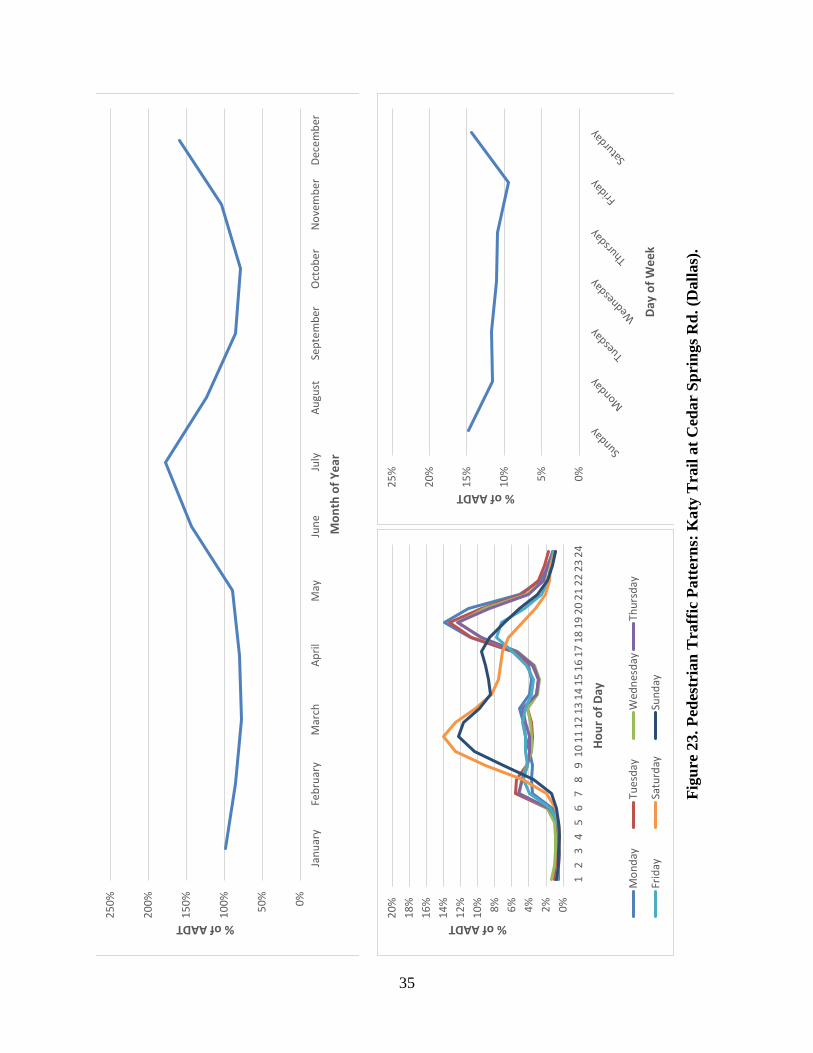
35

Figu

re 2

3. P

edes

tria

n T

raff

ic P

atte

rns:

Kat

y T

rail

at C

edar

Spr

ings

Rd.

(Dal

las)

.

0%50%

100%

150%

200%

250%

Janu

ary

Febr

uary

Mar

chAp

rilM

ayJu

neJu

lyAu

gust

Sept

embe

rO

ctob

erN

ovem

ber

Dece

mbe

r

% of AADT

Mon

th o

f Yea

r

0%2%4%6%8%10%

12%

14%

16%

18%

20%

12

34

56

78

910

1112

1314

1516

1718

1920

2122

2324

% of AADT

Hour

of D

ay

Mon

day

Tues

day

Wed

nesd

ayTh

ursd

ay

Frid

aySa

turd

aySu

nday

0%5%10%

15%

20%

25%

% of AADT

Day

of W

eek

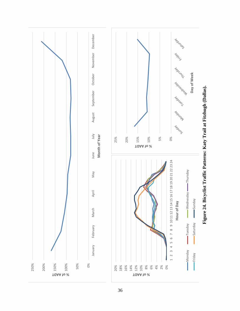
36

Figu

re 2

4. B

icyc

list T

raff

ic P

atte

rns:

Kat

y T

rail

at F

itzhu

gh (D

alla

s).

0%50%

100%

150%

200%

250%

Janu

ary

Febr

uary

Mar

chAp

rilM

ayJu

neJu

lyAu

gust

Sept

embe

rO

ctob

erN

ovem

ber

Dece

mbe

r

% of AADT

Mon

th o

f Yea

r

0%2%4%6%8%10%

12%

14%

16%

18%

20%

12

34

56

78

910

1112

1314

1516

1718

1920

2122

2324

% of AADT

Hour

of D

ay

Mon

day

Tues

day

Wed

nesd

ayTh

ursd

ay

Frid

aySa

turd

aySu

nday

0%5%10%

15%

20%

25%

% of AADT

Day

of W

eek

37

Figu

re 2

5. P

edes

tria

n T

raff

ic P

atte

rns:

Kat

y T

rail

at F

itzhu

gh (D

alla

s).

0%50%

100%

150%

200%

250%

Janu

ary

Febr

uary

Mar

chAp

rilM

ayJu

neJu

lyAu

gust

Sept

embe

rO

ctob

erN

ovem

ber

Dece

mbe

r

% of AADT

Mon

th o

f Yea

r

0%2%4%6%8%10%

12%

14%

16%

18%

20%

12

34

56

78

910

1112

1314

1516

1718

1920

2122

2324

% of AADT

Hour

of D

ay

Mon

day

Tues

day

Wed

nesd

ayTh

ursd

ay

Frid

aySa

turd

aySu

nday

0%5%10%

15%

20%

25%

% of AADT

Day

of W

eek

38

Figu

re 2

6. B

icyc

list T

raff

ic P

atte

rns:

Kat

y T

rail

at H

arva

rd A

venu

e (D

alla

s).

0%50%

100%

150%

200%

250%

Janu

ary

Febr

uary

Mar

chAp

rilM

ayJu

neJu

lyAu

gust

Sept

embe

rO

ctob

erN

ovem

ber

Dece

mbe

r

% of AADT

Mon

th o

f Yea

r

0%2%4%6%8%10%

12%

14%

16%

18%

20%

12

34

56

78

910

1112

1314

1516

1718

1920

2122

2324

% of AADT

Hour

of D

ay

Mon

day

Tues

day

Wed

nesd

ayTh

ursd

ay

Frid

aySa

turd

aySu

nday

0%5%10%

15%

20%

25%

% of AADT

Day

of W

eek

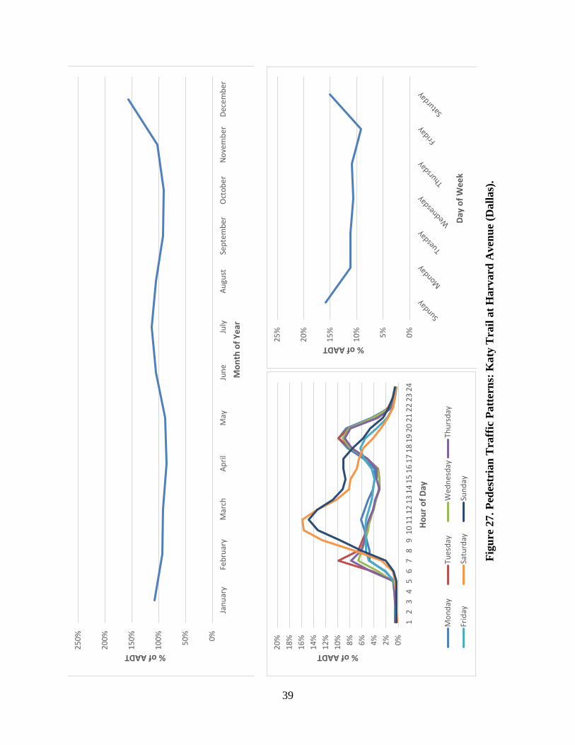
39

Figu

re 2

7. P

edes

tria

n T

raff

ic P

atte

rns:

Kat

y T

rail

at H

arva

rd A

venu

e (D

alla

s).

0%50%

100%

150%

200%

250%

Janu

ary

Febr

uary

Mar

chAp

rilM

ayJu

neJu

lyAu

gust

Sept

embe

rO

ctob

erN

ovem

ber

Dece

mbe

r

% of AADT

Mon

th o

f Yea

r

0%2%4%6%8%10%

12%

14%

16%

18%

20%

12

34

56

78

910

1112

1314

1516

1718

1920

2122

2324

% of AADT

Hour

of D

ay

Mon

day

Tues

day

Wed

nesd

ayTh

ursd

ay

Frid

aySa

turd

aySu

nday

0%5%10%

15%

20%

25%

% of AADT

Day

of W

eek

40

Figu

re 2

8. B

icyc

list T

raff

ic P

atte

rns:

Kat

y T

rail

(Hou

ston

Str

eet/A

A C

ente

r) (D

alla

s).

0%50%

100%

150%

200%

250%

Janu

ary

Febr

uary

Mar

chAp

rilM

ayJu

neJu

lyAu

gust

Sept

embe

rO

ctob

erN

ovem

ber

Dece

mbe

r

% of AADT

Mon

th o

f Yea

r

0%2%4%6%8%10%

12%

14%

16%

18%

20%

12

34

56

78

910

1112

1314

1516

1718

1920

2122

2324

% of AADT

Hour

of D

ay

Mon

day

Tues

day

Wed

nesd

ayTh

ursd

ay

Frid

aySa

turd

aySu

nday

0%5%10%

15%

20%

25%

% of AADT

Day

of W

eek

41

Figu

re 2

9. P

edes

tria

n T

raff

ic P

atte

rns:

Kat

y T

rail

(Hou

ston

Str

eet/A

A C

ente

r) (D

alla

s).

0%50%

100%

150%

200%

250%

Janu

ary

Febr

uary

Mar

chAp

rilM

ayJu

neJu

lyAu

gust

Sept

embe

rO

ctob

erN

ovem

ber

Dece

mbe

r

% of AADT

Mon

th o

f Yea

r

0%2%4%6%8%10%

12%

14%

16%

18%

20%

12

34

56

78

910

1112

1314

1516

1718

1920

2122

2324

% of AADT

Hour

of D

ay

Mon

day

Tues

day

Wed

nesd

ayTh

ursd

ay

Frid

aySa

turd

aySu

nday

0%5%10%

15%

20%

25%

% of AADT

Day

of W

eek

42

Figu

re 3

0. B

icyc

list T

raff

ic P

atte

rns:

Whi

te R

ock

Tra

il at

Big

Thi

cket

(Dal

las)

.

0%50%

100%

150%

200%

250%

Janu

ary

Febr

uary

Mar

chAp

rilM

ayJu

neJu

lyAu

gust

Sept

embe

rO

ctob

erN

ovem

ber

Dece

mbe

r

% of AADT

Mon

th o

f Yea

r

0%2%4%6%8%10%

12%

14%

16%

18%

20%

12

34

56

78

910

1112

1314

1516

1718

1920

2122

2324

% of AADT

Hour

of D

ay

Mon

day

Tues

day

Wed

nesd

ayTh

ursd

ay

Frid

aySa

turd

aySu

nday

0%5%10%

15%

20%

25%

% of AADT

Day

of W

eek

43

Figu

re 3

1. P

edes

tria

n T

raff

ic P

atte

rns:

Whi

te R

ock

Tra

il at

Big

Thi

cket

(Dal

las)

.

0%50%

100%

150%

200%

250%

Janu

ary

Febr

uary

Mar

chAp

rilM

ayJu

neJu

lyAu

gust

Sept

embe

rO

ctob

erN

ovem

ber

Dece

mbe

r

% of AADT

Mon

th o

f Yea

r

0%2%4%6%8%10%

12%

14%

16%

18%

20%

12

34

56

78

910

1112

1314

1516

1718

1920

2122

2324

% of AADT

Hour

of D

ay

Mon

day

Tues

day

Wed

nesd

ayTh

ursd

ay

Frid

aySa

turd

aySu

nday

0%5%10%

15%

20%

25%

% of AADT

Day

of W

eek

44

Figu

re 3

2. B

icyc

list T

raff

ic P

atte

rns:

Whi

te R

ock

Lak

e T

rail

(at F

ishe

r) (D

alla

s).

0%50%

100%

150%

200%

250%

Janu

ary

Febr

uary

Mar

chAp

rilM

ayJu

neJu

lyAu

gust

Sept

embe

rO

ctob

erN

ovem

ber

Dece

mbe

r

% of AADT

Mon

th o

f Yea

r

0%2%4%6%8%10%

12%

14%

16%

18%

20%

12

34

56

78

910

1112

1314

1516

1718

1920

2122

2324

% of AADT

Hour

of D

ay

Mon

day

Tues

day

Wed

nesd

ayTh

ursd

ay

Frid

aySa

turd

aySu

nday

0%5%10%

15%

20%

25%

% of AADT

Day

of W

eek

45

Fi

gure

33.

Ped

estr

ian

Tra

ffic

Pat

tern

s: W

hite

Roc

k L

ake

Tra

il (a

t Fis

her)

(Dal

las)

.

0%50%

100%

150%

200%

250%

Janu

ary

Febr

uary

Mar

chAp

rilM

ayJu

neJu

lyAu

gust

Sept

embe

rO

ctob

erN

ovem

ber

Dece

mbe

r

% of AADT

Mon

th o

f Yea

r

0%5%10%

15%

20%

25%

30%

12

34

56

78

910

1112

1314

1516

1718

1920

2122

2324

% of AADT

Hour

of D

ay

Mon

day

Tues

day

Wed

nesd

ayTh

ursd

ay

Frid

aySa

turd

aySu

nday

0

0.050.

1

0.150.

2

0.25

% of AADT

Day

of W

eek

46

Figu

re 3

4. B

icyc

list T

raff

ic P

atte

rns:

Whi

te R

ock

Lak

e T

rail

at W

infr

ey P

oint

(Dal

las)

.

0%50%

100%

150%

200%

250%

Janu

ary

Febr

uary

Mar

chAp

rilM

ayJu

neJu

lyAu

gust

Sept

embe

rO

ctob

erN

ovem

ber

Dece

mbe

r

% of AADT

Mon

th o

f Yea

r

0%2%4%6%8%10%

12%

14%

16%

18%

20%

12

34

56

78

910

1112

1314

1516

1718

1920

2122

2324

Axis

Title

Mon

day

Tues

day

Wed

nesd

ayTh

ursd

ay

Frid

aySa

turd

aySu

nday

0%5%10%

15%

20%

25%

% of AADT

Day

of W

eek

47

Figu

re 3

5. P

edes

tria

n T

raff

ic C

ount

Pat

tern

s: W

hite

Roc

k L

ake

Tra

il at

Win

frey

Poi

nt (D

alla

s).

0%50%

100%

150%

200%

250%

Janu

ary

Febr

uary

Mar

chAp

rilM

ayJu

neJu

lyAu

gust

Sept

embe

rO

ctob

erN

ovem

ber

Dece

mbe

r

% of AADT

Mon

th o

f Yea

r

0%5%10%

15%

20%

25%

30%

12

34

56

78

910

1112

1314

1516

1718

1920

2122

2324

% of AADT

Hour

of D

ay

Mon

day

Tues

day

Wed

nesd

ayTh

ursd

ay

Frid

aySa

turd

aySu

nday

0%5%10%

15%

20%

25%

% of AADT

Day

of W

eek

49

APPENDIX B. DEVELOPMENT OF PROCEDURES FOR CROWDSOURCED DATA SCALING

SELECTION OF MOST INFLUENTIAL VARIABLES

Researchers compiled a list of potentially important variables that can help to explain the relationships between the observed bicycle counts and Strava activity. Table 2 depicts the list of variables and data sources considered for the analysis.

Table 2. List of Variables Considered for the Analysis. Strava Manual American Community

Survey RHiNO

Edge ID Functional Class (CLAZZ) Activity Reverse Activity Weekend Ratio (both directions of travel) Morning Ratio (both directions of travel) Year Day Hour

Location ID City Station Name Latitude Longitude Station ID (both directions of travel) University (School) Present (0.5 miles radius) Functional Classification Facility Type Posted Speed Limit National Highway System Nonmotorized Facility Width Nonmotorized Facility Buffer Width Street Width Parking Pavement Type Pavement Condition ADA Ramps Street Lighting Street Traffic Volume (ADT) Transit

Total Population Male Population Male Population, in Various Age Groups Female Population Female Population, in Various Age Groups Total: Households Number of Households with Income:

• $10,000 • $10,000 to $14,999 • $15,000 to $19,999 • $20,000 to $24,999 • $25,000 to $29,999 • $30,000 to $34,999 • $35,000 to $39,999 • $40,000 to $44,999 • $45,000 to $49,999 • $50,000 to $59,999 • $60,000 to $74,999 • $75,000 to $99,999 • $100,000 to

$124,999 • $125,000 to

$149,999 • $150,000 to

$199,999 • > $200,000

Mode to Work: • Taxicab • Motorcycle • Bicycle

Street Name Highway Class Functional System Rural / Urban Current ADT K-Factor (Peak Hour) ADT Combined Left Shoulder Width Left Shoulder Type Right Shoulder Width Right Shoulder Type Median Width Median Type Number of Lanes Surface Width Left Curb Right Curb

50

Strava Sample Percentile Groups

Strava sample percentages refer to the ratio of Strava sample to observed bicycle counts:

𝑆𝑆𝑆𝑆𝑆𝑆𝑆𝑆𝑆𝑆𝑆𝑆 𝑆𝑆𝑆𝑆𝑆𝑆𝑆𝑆𝑊𝑊𝐶𝐶 𝑃𝑃𝐶𝐶𝑆𝑆𝑃𝑃𝐶𝐶𝑊𝑊𝑆𝑆𝑆𝑆𝑃𝑃𝐶𝐶𝑖𝑖 =𝑆𝑆𝑆𝑆𝑆𝑆𝑆𝑆𝑆𝑆𝑆𝑆 𝑆𝑆𝑆𝑆𝑆𝑆𝑆𝑆𝑊𝑊𝐶𝐶𝑖𝑖𝐴𝐴𝐵𝐵𝑃𝑃𝐵𝐵𝑃𝑃𝑊𝑊𝐶𝐶 𝐶𝐶𝐶𝐶𝑊𝑊𝑊𝑊𝑆𝑆𝐶𝐶𝑖𝑖

× 100%

Table 3 shows the descriptive statistics of Strava sample percentages for all locations.

Table 3. Descriptive Statistics of Strava Sample Percentages.

Percentage Strava Sample Min Max Mean St. D.

Travel Direction 1 0% 63% 5% 9%

Travel Direction 2 0% 55% 4% 8%

Average Sample Percentage 0% 59% 5% 8% Researchers categorized the Strava percentages into five groups, based on the percentiles. Table 4 reports the number of locations per percentile groups.

Table 4. Number of Locations per Percentile Groups.

Strava Percentile Group Number of Locations

Group 1 Less than 5% 73

Group 2 Equal and more than 5% and less than 10% 15

Group 3 Equal to or more than 10% and less than 15% 4

Group 4 Equal to or more than 15% and less than 20% 2

Group 5 Equal to or more than 20% 6

Total Number of Locations 153

Selection of Most Influential Factors

To select the most influential factors affecting the relationship between Strava activity and ground counts researchers used the Strava percentile groups and conducted the data mining analysis. For this purpose, researchers used Random Forest tool that helps to determine the most important variables based on two criteria:

51

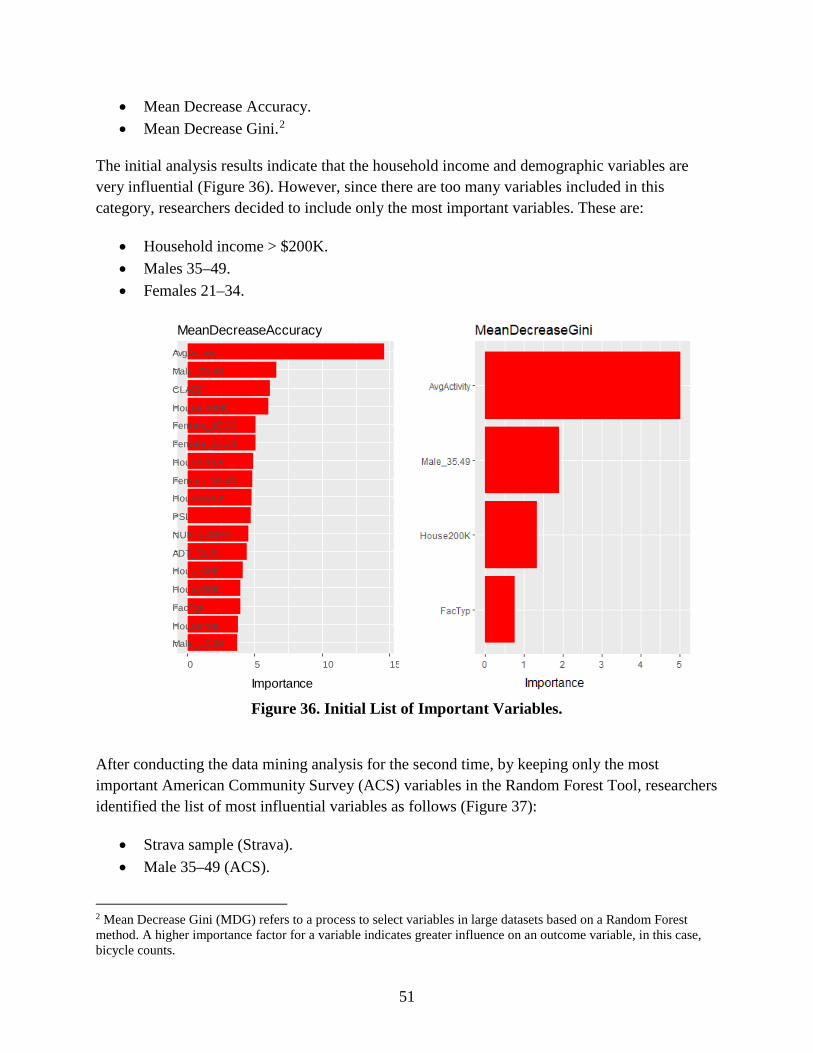
• Mean Decrease Accuracy. • Mean Decrease Gini.2

The initial analysis results indicate that the household income and demographic variables are very influential (Figure 36). However, since there are too many variables included in this category, researchers decided to include only the most important variables. These are:

• Household income > $200K. • Males 35–49. • Females 21–34.

Figure 36. Initial List of Important Variables.

After conducting the data mining analysis for the second time, by keeping only the most important American Community Survey (ACS) variables in the Random Forest Tool, researchers identified the list of most influential variables as follows (Figure 37):

• Strava sample (Strava). • Male 35–49 (ACS).

2 Mean Decrease Gini (MDG) refers to a process to select variables in large datasets based on a Random Forest method. A higher importance factor for a variable indicates greater influence on an outcome variable, in this case, bicycle counts.

Male_15.20

House40K

FacTyp

House50K

House30K

ADT_CUR

NUM_LANES

PSL

House125K

Female_35.49

House200K

Female_21.34

Female_15.20

House.200K

CLAZZ

Male_35.49

AvgActivity

0 5 10 15

MeanDecreaseAccuracy

Importance

52

• Household income of $200K (ACS). • Functional System, CLAZZ (Strava/OSM). • Number of Lanes (RHiNO). • Facility Type (Manual).

a) If both CLAZZ and FUN_SYS

included b) If only CLAZZ included

Figure 37. Final List of Important Variables. The CLAZZ variable indicates the roadway class. In this study, the researchers have used the ground counts collected from some of the roadway class types. However, Texas Strava shapefiles include other roadway classes that were not included in the study. Table 5 indicates the list of the roadway classes included in the Texas Strava (OSM) shapefiles, their definitions, default speeds and allowed transportation types (Source: Strava User Guide). The table also shows which of these roadway class types were included in the data analysis. The last column shows the corresponding roadway class types that can be used as a surrogate for the missing roadway classes. Note that the _link tags refer to the ramps and channelization. Since this roadway class was not included in the data analysis the coefficient for this category is zero. Moreover, the CLAZZ codes 43 and 74 have not been defined in the User Guide although they were included in the Texas Strava map. The coefficient for these types will also be equal to zero.

53

Table 5. CLAZZ Definitions. CLAZZ Codes in

Texas OSM

Definition Default Speed

(KMH)

Approximate Speed in

MPH

Allowed Transportation

Type

Included in the Model

Compatible CLAZZ

Code

11 Highway, motorway 120 75 Car No 15 12 Highway,

motorway_link* 30 20 Car No NA**

13 Highway, trunk 90 60 Car No 15 14 Highway, trunk_link* 30 20 Car No NA** 15 Highway, primary 70 45 Car Yes 15 16 Highway,

primary_link* 30 20 Car No NA**

21 Highway, secondary 60 40 Car Yes 21 22 Highway,

secondary_link* 30 20 Car No NA**

31 Highway, tertiary 40 25 Car, Bike Yes 31 32 Highway, residential 50 30 Car, Bike Yes 32 41 Highway, road 30 20 Car, Bike No 31 42 Highway, unclassified, 30 20 Car, Bike No 31 43 Not Defined 0 No 51 Highway, service 5 5 Car, Bike No 91/81 62 Highway, pedestrian 5 5 Bike, Foot No 91 63 Highway, living_street 7 5 Car, Bike, Foot No 91 71 Highway, track 10 10 Bike, Foot No 72 72 Highway, path 10 10 Bike, Foot Yes 72 73 Highway, bridleway 10 10 Bike, Foot No 72 74 Not Defined 0 No 81 Highway, cycleway 15 10 Bike Yes 81 91 Highway, footway 5 5 Foot Yes 91

*The _link tags are used to identify slip roads/ramps and "channelized" (physically separated) at-grade turning lanes connecting the through carriageways/through lanes of highways to other roadways of all types. _link tags

should also be used for physical channelization of turning traffic lanes at traffic signal junctions and in roundabout designs that physically separate a specific turn from the main roundabout (Source:

https://wiki.openstreetmap.org/wiki/Highway_link).

54

MODEL ESTIMATION RESULTS

After identifying the most important variables, researchers developed travel demand models to estimate the impact of these variables on the observed bicycle counts. Researchers developed two sets of models using:

• Strava and ACS databases (Model 1). • Strava, ACS and RHiNO databases (Model 2).

Each set of models consists of three models:

• Total Counts. • Default Direction Counts. • Reverse Direction Counts.

Hence a total of six models were developed to estimate the annual average daily bicycle (AADB) counts. Variable Males 35–49 was not included in the final models, since the sign of the variable kept changing based on the model. Researchers used the Strava Activity (AADB Strava), number of households with > 200K income (Households > 200K) and CLAZZ variables to develop Model 1.

Model 1 (CLAZZ) 𝐶𝐶𝐶𝐶𝐴𝐴𝐴𝐴𝑖𝑖 = exp (𝛽𝛽0 + 𝛽𝛽1 × 𝐶𝐶𝐶𝐶𝐴𝐴𝐴𝐴 𝑆𝑆𝑆𝑆𝑆𝑆𝑆𝑆𝑆𝑆𝑆𝑆𝑖𝑖 +

𝛽𝛽2 × Household > 200K 𝑖𝑖 + 𝛽𝛽3 × 𝐶𝐶𝐶𝐶𝐶𝐶𝐶𝐶𝐶𝐶𝑖𝑖)

Where

• 𝐶𝐶𝐶𝐶𝐴𝐴𝐴𝐴𝑖𝑖 − represents the estimated Annual Average Daily Bicycles at segments/edge 𝐵𝐵. • 𝐶𝐶𝐶𝐶𝐴𝐴𝐴𝐴 𝑆𝑆𝑆𝑆𝑆𝑆𝑆𝑆𝑆𝑆𝑆𝑆𝑖𝑖 − represents the Strava sample activity at location 𝐵𝐵 for the given time

period. • Household > 200K 𝑖𝑖 − represents the number of households with 200K income • 𝐶𝐶𝐶𝐶𝐶𝐶𝐶𝐶𝐶𝐶𝑖𝑖 − represents the functional system according to Strava/OSM. • 𝛽𝛽𝐶𝐶 − are the coefficient estimates.

Researchers used Strava Activity, number of households with > 200K income, FUN_SYS and number of lanes to develop Model 2. Model 2 (FUN_SYS) 𝐶𝐶𝐶𝐶𝐴𝐴𝐴𝐴𝑖𝑖 = exp (𝛽𝛽0 + 𝛽𝛽1 × 𝐶𝐶𝐶𝐶𝐴𝐴𝐴𝐴 𝑆𝑆𝑆𝑆𝑆𝑆𝑆𝑆𝑆𝑆𝑆𝑆𝑖𝑖 +

𝛽𝛽2 × Household > 200K 𝑖𝑖 + 𝛽𝛽3 × 𝐹𝐹𝐹𝐹𝐹𝐹_𝑆𝑆𝑆𝑆𝑆𝑆𝑖𝑖 + +𝛽𝛽4 × 𝐹𝐹𝐹𝐹𝑁𝑁_𝐶𝐶𝐶𝐶𝐹𝐹𝐿𝐿𝑆𝑆𝑖𝑖)

55

Where • 𝐶𝐶𝐶𝐶𝐴𝐴𝐴𝐴𝑖𝑖 − represents the estimated Annual Average Daily Bicycles at segments/edge 𝐵𝐵. • 𝐶𝐶𝐶𝐶𝐴𝐴𝐴𝐴 𝑆𝑆𝑆𝑆𝑆𝑆𝑆𝑆𝑆𝑆𝑆𝑆𝑖𝑖 − represents the Strava sample activity at location 𝐵𝐵 for the given time

period. • Household > 200K 𝑖𝑖 − represents the number of households with 200K income • 𝐹𝐹𝐹𝐹𝐹𝐹_𝑆𝑆𝑆𝑆𝑆𝑆𝑖𝑖 − represents the roadway functional system according to RHiNO • 𝐹𝐹𝐹𝐹𝑁𝑁_𝐶𝐶𝐶𝐶𝐹𝐹𝐿𝐿𝑆𝑆𝑖𝑖 − represents the number of lanes on the roadway segment. • 𝛽𝛽𝐶𝐶 − are the coefficient estimates.

Table 6 and Table 7 show the estimation results for both models, as well as the goodness of fit measures (overdispersion parameter and 𝑅𝑅2).

56

Tab

le 6

. Est

imat

ion

Res

ults

, Mod

el 1

. M

odel

1: 𝐶𝐶𝐶𝐶𝐴𝐴

𝐴𝐴 𝑖𝑖=

exp (𝛽𝛽 0

+𝛽𝛽 1

×𝐶𝐶𝐶𝐶

𝐴𝐴𝐴𝐴

𝑆𝑆𝑆𝑆𝑆𝑆𝑆𝑆𝑆𝑆𝑆𝑆 𝑖𝑖

+𝛽𝛽 2

×H

ouse

hold

>$2

00K 𝑖𝑖

+𝛽𝛽 3

×𝐶𝐶𝐶𝐶𝐶𝐶𝐶𝐶𝐶𝐶 𝑖𝑖

+𝜀𝜀 𝑖𝑖

)

Var

iabl

es In

clud

ed in

the

Mod

els

Tot

al C

ount

s D

efau

lt D

irec

tion

Cou

nts

Rev

erse

Dir

ectio

n C

ount

s

Est

imat

e St

.D.

p-va

lue

Est

imat

e St

.D.

p-va

lue

Est

imat

e St

.D.

p-va

lue

Inte

rcep

t (C

LAZZ

) H

ighw

ay, p

rimar

y 4.

138

0.05

3 <

0.00

1 2.

782

0.10

9 <

0.00

1 4.

343

0.04

1 <

0.00

1

Hig

hway

, se

cond

ary

2.59

0 0.

060

< 0.

001

2.59

8 0.

060

< 0.

001

2.52

1 0.

061

< 0.

001

Hig

hway

, ter

tiary

3.

078

0.06

2 <

0.00

1 3.

227

0.05

8 <

0.00

1 2.

830

0.06

8 <

0.00

1

Hig

hway

, re

side

ntia

l 2.

862

0.03

7 <

0.00

1 3.

184

0.03

2 <

0.00

1 2.

460

0.04

5 <

0.00

1

Hig

hway

, pat

h 4.

271

0.03

1 <

0.00

1 4.

551

0.02

9 <

0.00

1 3.

468

0.03

9 <

0.00

1

Cyc

lew

ay

4.14

4 0.

027

< 0.

001

4.13

4 0.

027

< 0.

001

3.75

4 0.

032

< 0.

001

Foot

way

3.

323

0.06

2 <

0.00

1 3.

468

0.06

0 <

0.00

1 2.

135

0.07

1 <

0.00

1

AA

DB

Stra

va

0.03

8 0.

000

< 0.

001

0.02

2 0.

000

< 0.

001

0.10

0 0.

001

< 0.

001

Num

ber o

f Hou

seho

lds w

ith >

200K

in

com

e 0.

002

0.00

0 <

0.00

1 0.

002

0.00

0 <

0.00

1 0.

000

0.00

0 <

0.01

𝑅𝑅2 (M

odel

Acc

urac

y)

75%

85

%

83%

Ove

rdis

pers

ion

1.17

2 0.

822

1.33

8

57

Tab

le 7

. Est

imat

ion

Res

ults

, Mod

el 2

. M

odel

2: 𝐶𝐶𝐶𝐶𝐴𝐴

𝐴𝐴 𝑖𝑖=

exp (𝛽𝛽 0

+𝛽𝛽 1

×𝐶𝐶𝐶𝐶

𝐴𝐴𝐴𝐴

𝑆𝑆𝑆𝑆𝑆𝑆𝑆𝑆𝑆𝑆𝑆𝑆 𝑖𝑖

+𝛽𝛽 2

×H

ouse

hold

> 2

00K 𝑖𝑖

+𝛽𝛽 3

×𝐹𝐹𝐹𝐹

𝐹𝐹_𝑆𝑆𝑆𝑆𝑆𝑆

𝑖𝑖+

+𝛽𝛽 4

×𝐹𝐹𝐹𝐹𝑁𝑁

_𝐶𝐶𝐶𝐶𝐹𝐹

𝐿𝐿𝑆𝑆𝑖𝑖

+𝜀𝜀 𝑖𝑖

)

Var

iabl

es In

clud

ed in

the

Mod

els

Tot

al C

ount

s D

efau

lt D

irec

tion

Cou

nts

Rev

erse

Dir

ectio

n C

ount

s E

stim

ate

St.D

. p-

valu

e E

stim

ate

St.D

. p-

valu

e E

stim

ate

St.D

. p-

valu

e In

terc

ept

(FU

N_S

YS)

C

olle

ctor

(M

inor

) 3.

211

0.07

8 <

0.00

1 2.

491

0.09

4 <

0.00

1 3.

078

0.08

2 <

0.00

1

Loca

l Roa

d 2.

506

0.08

3 <

0.00

1 1.

631

0.09

2 <

0.00

1 3.

036

0.07

7 <

0.00

1

Min

or A

rteria

l 2.

987

0.11

8 <

0.00

1 1.

548

0.13

9 <

0.00

1 3.

662

0.10

2 <

0.00

1

Prin

cipa

l A

rteria

l 3.

929

0.11

6 <

0.00

1 1.

539

0.16

2 <

0.00

1 4.

741

0.08

8 <

0.00

1

Trai

l 4.

270

0.03

5 <

0.00

1 4.

047

0.03

8 <

0.00

1 3.

969

0.03

5 <

0.00

1

AA

DB

Stra

va

0.03

1 0.

000

< 0.

001

0.01

7 0.

000

< 0.

001

0.09

1 0.

001

< 0.

001

Den

sity

of H

ouse

hold

s with

>20

0K

inco

me

0.00

2 0.

000

< 0.

001

0.00

2 0.

000

< 0.

001

0.00

0 0.

000

< 0.

001

Num

ber o

f Lan

e -0

.066

0.

027

< 0.

05

0.31

0 0.

032

< 0.

001

-0.2

71

0.02

3 <

0.00

1

𝑅𝑅2 (M

odel

Acc

urac

y)

70%

64

%

70%

Ove

rdis

pers

ion

0.96

7 0.

734

1.12

9

58

PREDICTION ERROR MEASURES

Figure 38 indicates the prediction intervals.

a) Model 1 b) Model 2 Figure 38. Prediction Intervals.

In addition to the prediction intervals, researchers calculated three prediction error measures to test the prediction accuracy of each model.

Mean Absolute Percentage Error

𝑁𝑁𝐶𝐶𝑃𝑃𝐿𝐿 =1𝑊𝑊� 100 × �

𝑆𝑆�𝑃𝑃𝑁𝑁𝑆𝑆,𝑆𝑆 − 𝑆𝑆𝑃𝑃𝑁𝑁𝑆𝑆 ,𝑆𝑆

𝑆𝑆𝑃𝑃𝑁𝑁𝑆𝑆,𝑆𝑆�

𝑊𝑊

Mean Accuracy Error

𝑁𝑁𝐶𝐶𝐿𝐿 =1𝑊𝑊� �𝑆𝑆�𝑃𝑃𝑁𝑁𝑆𝑆 ,𝑆𝑆 − 𝑆𝑆𝑃𝑃𝑁𝑁𝑆𝑆,𝑆𝑆�

𝑊𝑊

Mean Squared Error

𝑁𝑁𝑆𝑆𝐿𝐿 =1𝑊𝑊� �𝑆𝑆�𝑃𝑃𝑁𝑁𝑆𝑆 ,𝑆𝑆 − 𝑆𝑆𝑃𝑃𝑁𝑁𝑆𝑆 ,𝑆𝑆�

2

𝑊𝑊

Where,

• 𝑊𝑊 − is the size of the validation data (four months). • 𝑆𝑆𝑃𝑃𝑃𝑃,𝑊𝑊 − is the performance measures vector for period 𝑆𝑆, where 𝑆𝑆 = 1,𝑇𝑇. • 𝑆𝑆�𝑃𝑃𝑃𝑃𝑝𝑝,𝑊𝑊 − is the predicted value of the performance measure.

59

Table 8 reports the error measures for the two models while Table 9 shows the error measures for the Strava percentile groups listed in Table 3. Note that in this table the percentages refer to the error rate and not the accuracy. Hence, the higher the value, the higher the prediction error. According to the error rates, the prediction power of both models are quite similar. Moreover, the accuracy is better for the roadway segments where the Strava sample represents 5–15 percent of bicycle counts (Groups 2 and 3).

Table 8. Relative Accuracy per Strava Percentage Categories.

Prediction Error Measure Model 1 (CLAZZ)

Model 2 (RHiNO)

Mean Absolute Percentage Error 29% 38%

Mean Squared Error 5855 4836

Mean Absolute Error 41 42

Table 9. Prediction Error per Strava Percentile Groups.

Strava Percentile Groups Mean Absolute Prediction Error Mean Squared Error Mean Absolute Error

Model 1 (CLAZZ)

Model 2 (RHiNO)

Model 1 (CLAZZ)

Model 2 (RHiNO)

Model 1 (CLAZZ)

Model 2 (RHiNO)

Group 1 Strava Ratio < 5% 33% 44% 3066 3500 30 33

Group 2 5% ≤ Strava Ratio < 10% 9.80% 12.50% 5686 7501 59 67

Group 3 10% ≤ Strava Ratio < 15% 9.90% 10.10% 9894 2390 66 103

Group 4 15% ≤ Strava Ratio < 20% 42% 46% 3557 5154 49 68

Group 5 20% ≤ Strava Ratio 38% 39.70% 38286 1606 104 34

Average 29% 38% 5855 4836 41 42

Table 10 reports the observed and predicted counts and the lower and upper prediction intervals based on Model 1 (which uses CLAZZ to represent functional class).

60

Tab

le 1

0. P

redi

ctio

n In

terv

als B

ased

on

Mod

el 1

(CL

AZ

Z fu

nctio

nal c

lass

). St

atio

n N

ame

City

C

LA

ZZ

St

rava

A

AD

B

Obs

erve

d A

AD

B

Pred

icte

d A

AD

B

Low

er

Pred

ictio

n In

terv

al

(95%

)

Upp

er

Pred

ictio

n In

terv

al

(95%

) A

nn a

nd R

oy B

utle

r Tra

il @

E

Bou

ldin

Cre

ek

Aus

tin

81

35

791

238

168

308

Ann

and

Roy

But

ler T

rail

@ M

oPac

Ex

py

Aus

tin

81

52

660

455

385

525

Duv

al S

t N o

f E 3

2nd

St

Aus

tin

31

11

376

33

0 10

3

Gua

dalu

pe S

t N o

f W 2

1st S

t A

ustin

15

20

28

1 13

4 64

20

4 Jo

hnso

n C

reek

Tra

il @

MoP

ac/W

5th

St

/W 6

th S

t Int

erch

ange

A

ustin

81

1

108

65

0 13

5

Lanc

e A

rmst

rong

Bik

eway

@ W

alle

r C

reek

A

ustin

81

55

10

71

510

440

580

Man

or R

d @

Ala

mo

St

Aus

tin

21

17

288

25

0 95

S 1s

t St @

S B

ank

Col

orad

o R

iver

A

ustin

81

36

24

1 24

8 17

8 31

8

Shoa

l Cre

ek B

lvd

N o

f W 2

4th

St

Aus

tin

91

43

162

130

60

200

Shoa

l Cre

ek B

lvd

N o

f W 3

8th

St

Aus

tin

31

8 20

29

0

99

Wal

nut C

reek

Tra

il N

of J

ain

Ln

Aus

tin

81

45

304

349

279

419

Old

Alic

e R

oad

at N

of B

elve

dere

B

row

nsvi

lle

32

10

148

26

0 96

FM 8

02 a

t W o

f Hab

ana

Bro

wns

ville

15

2

57

68

0 13

8

FM 8

02 a

t W o

f Hab

ana

Bro

wns

ville

15

0

38

63

0 13

3

Spor

ts P

ark

Blv

d at

W o

f B

row

nsvi

lle S

ports

Par

k B

row

nsvi

lle

32

0 7

17

0 87

18th

: Fig

to M

cKen

zie

C

orpu

s Chr

isti

32

0 19

17

0

87

Ala

med

a: A

tlant

ic to

Nap

les

Cor

pus C

hris

ti 21

0

2 13

0

83

61

Stat

ion

Nam

e C

ity

CL

AZ

Z

Stra

va

AA

DB

O

bser

ved

AA

DB

Pr

edic

ted

AA

DB

Low

er

Pred

ictio

n In

terv

al

(95%

)

Upp

er

Pred

ictio

n In

terv

al

(95%

)

Ala

med

a: M

usse

tt to

Cal

dwel

l C

orpu

s Chr

isti

32

0 11

17

0

87

Ala

med

a: N

aple

s to

Atla

ntic

C

orpu

s Chr

isti

21

0 6

13

0 83

Am

ber:

J to

Don

Pat

ricio

C

orpu

s Chr

isti

32

0 11

17

0

87

Ant

elop

e: A

rtesi

an to

Car

rizo

C

orpu

s Chr

isti

21

0 11

13

0

83

Aqu

ariu

s: D

oubl

oon

to G

unw

ale

C

orpu

s Chr

isti

32

0 27

17

0

87

Aye

rs: 2

nd to

3rd

C

orpu

s Chr

isti

21

0 8

13

0 83

Aye

rs: 3

rd to

2nd

C

orpu

s Chr

isti

21

0 11

13

0

83

Aye

rs: 6

th to

7th

C

orpu

s Chr

isti

21

0 9

13

0 83

Aye

rs: 7

th to

6th

C

orpu

s Chr

isti

21

0 6

13

0 83

Bea

uvai

s: G

rena

de to

Bea

u Te

rre

C

orpu

s Chr

isti

32

1 16

18

0

88

Ber

nice

: Ric

key

to S

usan

C

orpu

s Chr

isti

32

1 12

18

0

88

Ble

vins

: Orm

ond

to M

elbo

urne

C

orpu

s Chr

isti

32

0 44

17

0

87

Bro

ckha

mpt

on: D

unba

rton

Oak

to L

a R

oche

lle W

ay

Cor

pus C

hris

ti 31

1

13

23

0 93

Buf

ord:

23r

d to

22n

d

Cor

pus C

hris

ti 32

0

21

17

0 87

Buf

ord:

San

ta F

e to

3rd

C

orpu

s Chr

isti

32

0 10

17

0

87

62

Stat

ion

Nam

e C

ity

CL

AZ

Z

Stra

va

AA

DB

O

bser

ved

AA

DB

Pr

edic

ted

AA

DB

Low

er

Pred

ictio

n In

terv

al

(95%

)

Upp

er

Pred

ictio

n In

terv

al

(95%

)

Car

roll:

Car

rolle

ton

to G

ollih

ar

Cor

pus C

hris

ti 31

0

13

22

0 92

Car

roll:

Gol

lihar

to C

arro

lleto

n

Cor

pus C

hris

ti 31

0

8 22

0

92

Car

roll:

Lam

ont t

o H

arol

d

Cor

pus C

hris

ti 31

0

12

22

0 92

Car

roll:

Lam

ont t

o M

ario

n (#

1)

Cor

pus C

hris

ti 31

0

15

22

0 92

Car

roll:

Lam

ont t

o M

ario

n (#

2)

Cor

pus C

hris

ti 31

0

13

22

0 92

Cen

ter:

Pasa

dena

to P

eerm

an

Cor

pus C

hris

ti 32

1

30

18

0 88

Che

yenn

e: A

ztec

to W

ashi

ngto

n

Cor

pus C

hris

ti 32

0

10

17

0 87

Clif

f Cre

nsha

w: G

uess

to T

urke

y C

reek

C

orpu

s Chr

isti

32

1 65

18

0

88

Cor

ona:

Em

bass

y to

Fly

nn P

arkw

ay

Cor

pus C

hris

ti 31

0

6 22

0

92

Cor

ona:

Fly

nn P

arkw

ay to

Em

bass

y

Cor

pus C

hris

ti 31

0

6 22

0

92

Gol

lihar

: Dod

y to

Web

er

Cor

pus C

hris

ti 21

0

8 13

0

83

Gol

lihar

: Drif

twoo

d to

Dol

phin

C

orpu

s Chr

isti

21

0 4

13

0 83

Gol

lihar

: Kas

per t

o W

eber

C

orpu

s Chr

isti

21

0 2

13

0 83

Gol

lihar

: Lau

ra to

Kirk

woo

d

Cor

pus C

hris

ti 21

0

11

13

0 83

Gol

lihar

: Lau

ra to

Ran

dall

C

orpu

s Chr

isti

21

0 33

13

0

83

63

Stat

ion

Nam

e C

ity

CL

AZ

Z

Stra

va

AA

DB

O

bser

ved

AA

DB

Pr

edic

ted

AA

DB

Low

er

Pred

ictio

n In

terv

al

(95%

)

Upp

er

Pred

ictio

n In

terv

al

(95%

)

Gol

lihar

: Seq

uoia

to W

illow

C

orpu

s Chr

isti

21

0 4

13

0 83

Gyp

sy: H

awks

nest

Bay

to W

hale

r C

orpu

s Chr

isti

32

0 15

17

0

87

Hol

ly: S

H 2

86 to

Mar

tin

Cor

pus C

hris

ti 21

0

55

13

0 83

Hol

ly: V

icto

r Lar

a O

rtego

n to

G

reen

woo

d

Cor

pus C

hris

ti 21

0

17

13

0 83

Law

nvie

w: S

unse

t to

Mel

rose

C

orpu

s Chr

isti

32

0 20

17

0

87

Mat

lock

: Gre

enba

y to

Mci

ver

Cor

pus C

hris

ti 32

0

46

17

0 87

Mes

quite

: Fitz

gera

ld to

Res

aca

C

orpu

s Chr

isti

32

0 26

17

0

87

Peop

les:

Cha

ppar

al to

Mes

quite

C

orpu

s Chr

isti

32

0 17

17

0

87

Pont

char

train

: Kaw

Lak

e to

Lak

e Tr

avis

C

orpu

s Chr

isti

32

1 9

18

0 88

Ret

ta: P

urdu

e to

Sel

kirk

C

orpu

s Chr

isti

31

0 27

22

0

92

Riv

er C

anyo

n: T

eagu

e to

Rol

ling

Rid

ge

Cor

pus C

hris

ti 32

0

30

17

0 87

Rod

d Fi

eld:

Sar

atog

a to

Bro

oke

C

orpu

s Chr

isti

21

0 59

13

0

83

Roo

seve

lt: C

lark

to V

ande

rbilt

C

orpu

s Chr

isti

32

0 17

17

0

87

Sabi

nas:

Dun

bar t

o Ta

rlton

C

orpu

s Chr

isti

32

0 7

17

0 87

Woo

d R

iver

: Red

Riv

er to

Rap

ids

Cor

pus C

hris

ti 32

1

52

18

0 88

64

Stat

ion

Nam

e C

ity

CL

AZ

Z

Stra

va

AA

DB

O

bser

ved

AA

DB

Pr

edic

ted

AA

DB

Low

er

Pred

ictio

n In

terv

al

(95%

)

Upp

er

Pred

ictio

n In

terv

al

(95%

)

Yor

ktow

n: G

reat

Lak

es to

Oso

Pa

rkw

ay

Cor

pus C

hris

ti 21

2

12

14

0 84

AT&

T Tr

ail a

t Trin

ity F

ores

t Tra

il

Dal

las

72

0 16

72

2

142

Coo

mbs

Cre

ek T

rail

D

alla

s 81

4

19

73

3 14

3

Gat

eway

Par

k Lo

op T

rail

D

alla

s 91

0

68

25

0 95

Gle

ndal

e Pa

rk L

oop

Trai

l

Dal

las

91

0 20

25

0

95

Gle

ndal

e Pa

rk S

outh

Loo

p Tr

ail

Dal

las

91

0 29

25

0

95

Kat

y Tr

ail (

Hou

ston

stre

et/ A

A

Cen

ter-

D

alla

s 81

15

41

9 11

1 41

18

1

Kat

y Tr

ail a

t Ced

ar S

prin

gs R

d

Dal

las

81

28

537

183

113

253

Kat

y Tr

ail a

t Fitz

hugh

D

alla

s 81

26

57

7 16

9 99

23

9

Kat

y Tr

ail a

t Har

vard

Ave

nue

D

alla

s 81

19

32

7 13

0 60

20

0 K

iest

Par

k Lo

op T

rail

at

Con

serv

atio

n

Dal

las

81

0 73

63

0

133

Pres

ton

Rid

ge T

rail

at L

a C

osa

Dr.

D

alla

s 81

6

7 79

9

149

Pres

ton

Rid

ge T

rial a

t Deb

be

Dal

las

72

6 83

90

20

16

0

Trin

ity st

rand

Tra

il at

Hi L

ine

Dr

Dal

las

91

0 20

25

0

95

W N

orth

Wes

t Hig

hway

D

alla

s 15

0

66

63

0 13

3

Whi

te R

ock

Lake

Tra

il

Dal

las

72

23

532

172

102

242

Whi

te R

ock

Lake

Tra

il at

Win

frey

Po

int

Dal

las

81

151

1337

19

575

1950

5 19

645

Whi

te R

ock

Trai

l at B

ig T

hick

et

Dal

las

32

161

1214

79

43

7873

80

13

Whi

te R

ock

Trai

l at D

og P

ark

D

alla

s 72

53

70

9 53

6 46

6 60

6 B

rays

Bay

ou G

reen

way

Tra

il @

Spu

r 5

H

oust

on

72

4 65

83

13

15

3

Col

umbi

a Ta

p Tr

ail @

Blo

dget

t St

reet

H

oust

on

81

4 12

1 73

3

143

65

Stat

ion

Nam

e C

ity

CL

AZ

Z

Stra

va

AA

DB

O

bser

ved

AA

DB

Pr

edic

ted

AA

DB

Low

er

Pred

ictio

n In

terv

al

(95%

)

Upp

er

Pred

ictio

n In

terv

al

(95%

)

Hei

ghts

Tra

il @

5 1/

2 St

reet

H

oust

on

72

26

599

192

122

262

Whi

te O

ak B

ayou

Tra

il@ 3

4th

Stre

et

Hou

ston

72

33

20

4 25

1 18

1 32

1

SH 3

N @

S o

f Wal

ter H

all P

ark

Le

ague

City

15

4

258

73

3 14

3

Mid

Col

lege

Cha

parr

al C

reek

Bik

e La

ne S

outh

Sid

e M

idla

nd

32

0 15

17

0

87

Oak

woo

d D

r at W

of S

unny

grov

e D

r O

dess

a 32

0

2 17

0

87

Map

le A

ve a

t S o

f E 1

4th

St

Ode

ssa

32

0 2

17

0 87

W 2

2nd

St a

t Ven

tura

Ave

O

dess

a 32

0

2 17

0

87

Plan

o B

lueb

onne

t Tra

il at

US7

5

Plan

o 91

4

5 29

0

99

Plan

o Le

gacy

Tra

il

Plan

o 72

9

10

101

31

171

Plan

o O

PP &

NP

Trai

l Pl

ano

72

1 53

74

4

144

Mis

sion

Rea

ch T

rail

at n

orth

end

of

San

Juan

Ditc

h

San

Ant

onio

81

1

30

65

0 13

5

Mis

sion

Rea

ch T

rail

sout

h of

The

o A

ve

San

Ant

onio

81

6

148

79

9 14

9

Mis

sion

Rea

ch T

rail

sout

h of

VFW

B

lvd

(Mis

sion

Cou

nty

Park

) Sa

n A

nton

io

81

3 61

71

1

141

Riv

erw

alk

Trai

l bet

wee

n 8t

h an

d 9t

h St

reet

Sa

n A

nton

io

91

11

225

38

0 10

8

Wic

hita

Riv

er T

rail

at E

of B

road

St

/IH-4

4 W

ichi

ta F

alls

81

0

40

63

0 13

3

FM 3

69 a

t N o

f US

287

Wic

hita

Fal

ls

21

0 2

13

0 83

Bur

kbur

nett

Rd

(SH

240

) at N

of

Airp

ort D

r W

ichi

ta F

alls

21

2

3 14

0

84