Eurostat

Seasonal Adjustment

Topics

• Motivation and theoretical background (Øyvind Langsrud)

• Seasonal adjustment step-by-step (László Sajtos)

• (A few) issues on seasonal adjustment (László Sajtos)

Presented by

• Øyvind Langsrud

• Statistics Norway

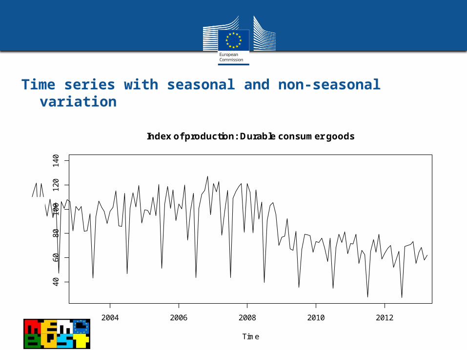
Time series with seasonal and non-seasonal variation

Index of production: Durable consumer goods

Time

a1

2004 2006 2008 2010 2012

40

60

80

10

01

20

14

0

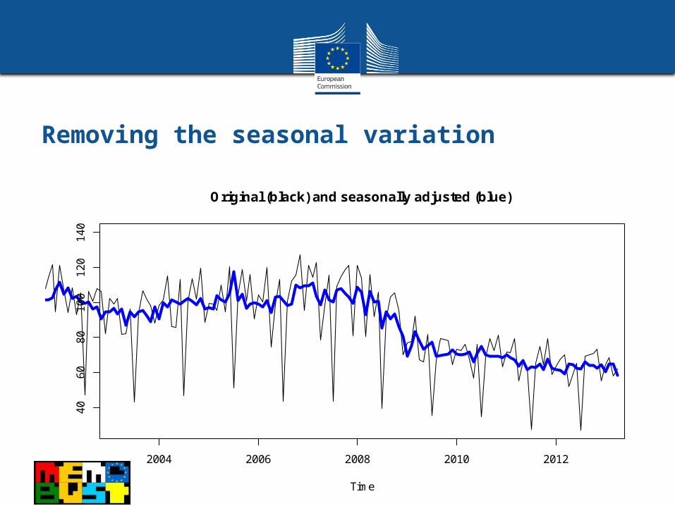
Removing the seasonal variation

Original (black) and seasonally adjusted (blue)

Time

2004 2006 2008 2010 2012

40

60

80

10

01

20

14

0

Removing also the non-seasonal variation

Original (black), seasonally adjusted (blue) and trend (red)

Time

2004 2006 2008 2010 2012

40

60

80

10

01

20

14

0

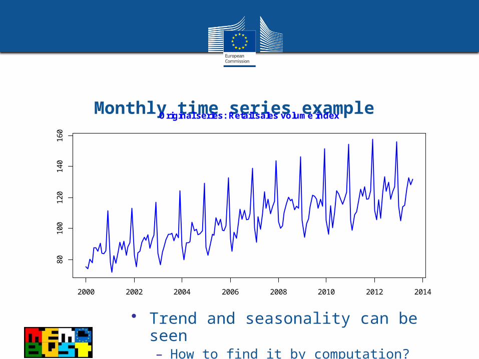
Monthly time series example

• Trend and seasonality can be seen – How to find it by computation?

Original series: Retail sales volume index

2000 2002 2004 2006 2008 2010 2012 2014

80

10

01

20

14

01

60

2000 2002 2004 2006 2008 2010 2012 2014

80

10

01

20

14

01

60

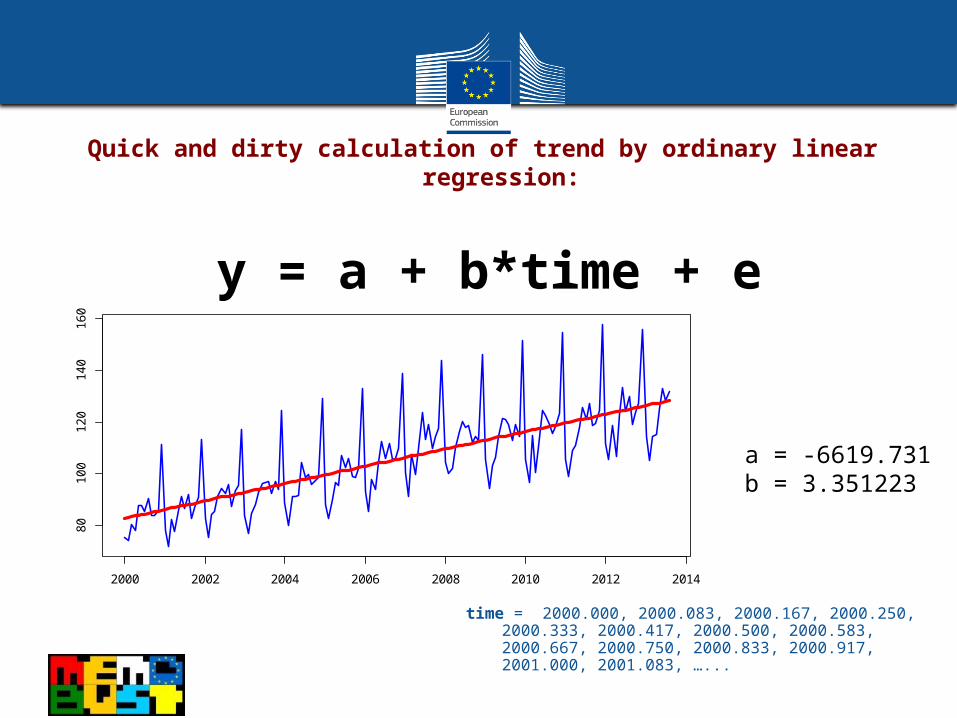
Quick and dirty calculation of trend by ordinary linear regression:

y = a + b*time + e

time = 2000.000, 2000.083, 2000.167, 2000.250, 2000.333, 2000.417, 2000.500, 2000.583, 2000.667, 2000.750, 2000.833, 2000.917, 2001.000, 2001.083, …...

a = -6619.731 b = 3.351223

Original (blue) and model fit (red)

2000 2002 2004 2006 2008 2010 2012 2014

80

10

01

20

14

01

60

Including seasonality in "the dirty model"

y = a + b*time + cmonth + e

Original (blue) and model fit (red)

2000 2002 2004 2006 2008 2010 2012 2014

8010

012

014

016

0

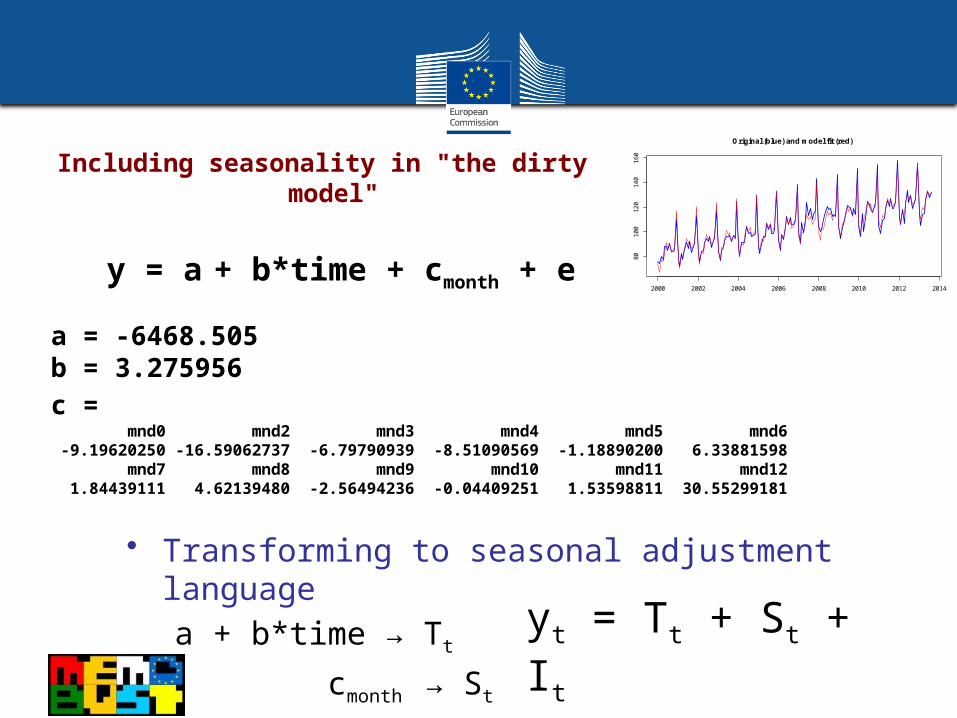
Including seasonality in "the dirty model"

y = a + b*time + cmonth + e

a = -6468.505b = 3.275956 c = mnd0 mnd2 mnd3 mnd4 mnd5 mnd6 -9.19620250 -16.59062737 -6.79790939 -8.51090569 -1.18890200 6.33881598 mnd7 mnd8 mnd9 mnd10 mnd11 mnd12 1.84439111 4.62139480 -2.56494236 -0.04409251 1.53598811 30.55299181

• Transforming to seasonal adjustment languagea + b*time → Tt

cmonth → St

e → It

yt = Tt + St + It

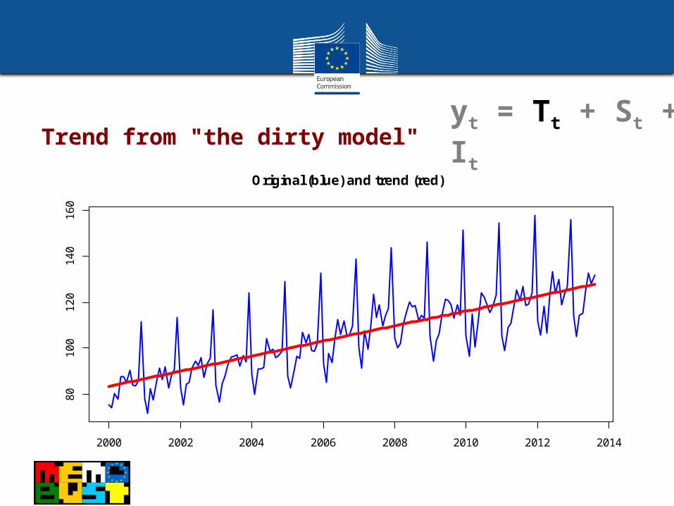
Trend from "the dirty model" Original (blue) and trend (red)

2000 2002 2004 2006 2008 2010 2012 2014

80

10

01

20

14

01

60

yt = Tt + St + It

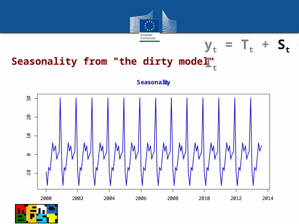
Seasonality from "the dirty model" yt = Tt + St + It

Seasonality

2000 2002 2004 2006 2008 2010 2012 2014

-10

01

02

03

0

Seasonal adjustment by "the dirty model"

yt = Tt + St + It

Original (blue) and seasonal adjusted (red)

2000 2002 2004 2006 2008 2010 2012 2014

80

10

01

20

14

01

60

Question to the audience:

What is wrong with this ordinary regression approach ?

Irregular component by "the dirty model"

yt = Tt + St + It

Irregular componet

2000 2002 2004 2006 2008 2010 2012 2014

-50

51

0

Original (blue) and trend (red)

2000 2002 2004 2006 2008 2010 2012 2014

80

10

01

20

14

01

60

In practise a multiplicative model is used: yt = Tt × St × It

• yt is not the original series but a series that is corrected for holiday and trading day effects (calendar adjusted)

yt = Tt × St × It

yt = Tt × St × It

• Note that the seasonal factors vary slightly along time

Seasonal factors

2000 2005 2010 2015

0.9

1.0

1.1

1.2

1.3

Irregular componet

2000 2002 2004 2006 2008 2010 2012 2014

0.9

70

.98

0.9

91

.00

1.0

11

.02

yt = Tt × St × It

• This time the irregular component looks more as true noise

• Note that correlated neighbour values is allowed (autocorrelation)

Original (blue) and seasonally adjusted (red)

2000 2002 2004 2006 2008 2010 2012 2014

80

10

01

20

14

01

60

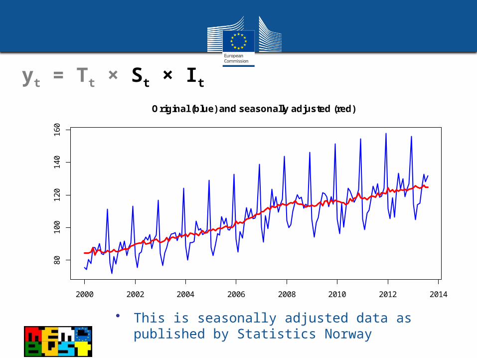
yt = Tt × St × It

• This is seasonally adjusted data as published by Statistics Norway

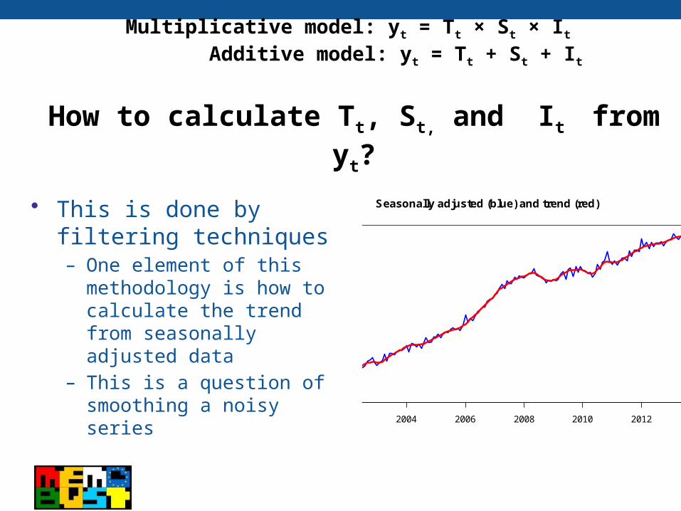
Multiplicative model: yt = Tt × St × It Additive model: yt = Tt + St + It

How to calculate Tt, St, and It from yt?

Seasonally adjusted (blue) and trend (red)

2000 2002 2004 2006 2008 2010 2012 2014

90

10

01

10

12

0

• This is done by filtering techniques– One element of this

methodology is how to calculate the trend from seasonally adjusted data

– This is a question of smoothing a noisy series

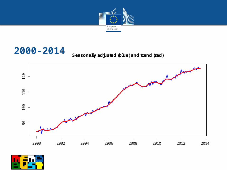
2000-2014Seasonally adjusted (blue) and trend (red)

2000 2002 2004 2006 2008 2010 2012 2014

90

10

01

10

12

0

2007-2012 Seasonally adjusted (blue) and trend (red)

2007 2008 2009 2010 2011 2012

11

01

15

12

0

Smoothing by averaging • Pt = (Yt-1+ Yt + Yt+1)/3

3-term simple moving average: [1,1,1]/3

2007 2008 2009 2010 2011 2012

11

01

15

12

0

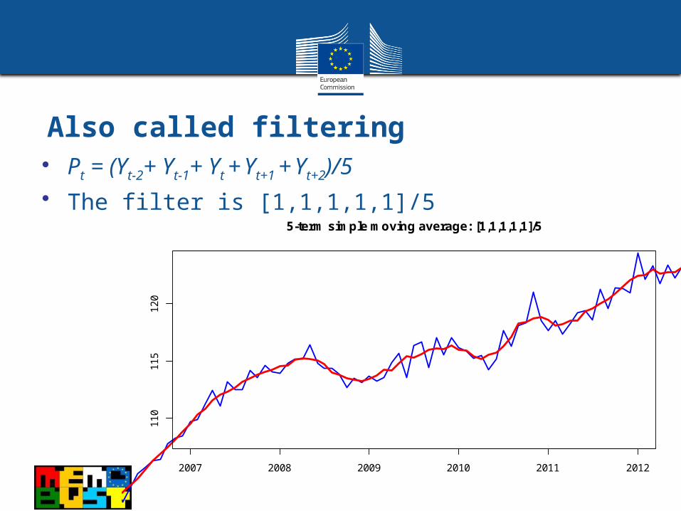
Also called filtering • Pt = (Yt-2+ Yt-1+ Yt + Yt+1 + Yt+2)/5• The filter is [1,1,1,1,1]/5

5-term simple moving average: [1,1,1,1,1]/5

2007 2008 2009 2010 2011 2012

11

01

15

12

0

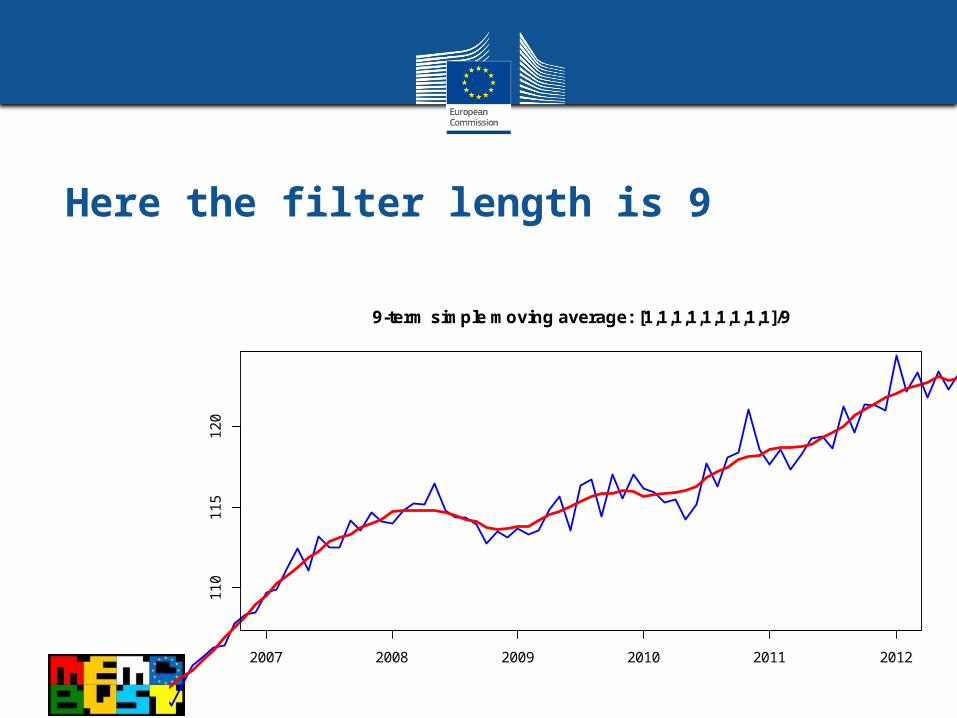
Here the filter length is 9

9-term simple moving average: [1,1,1,1,1,1,1,1,1]/9

2007 2008 2009 2010 2011 2012

11

01

15

12

0

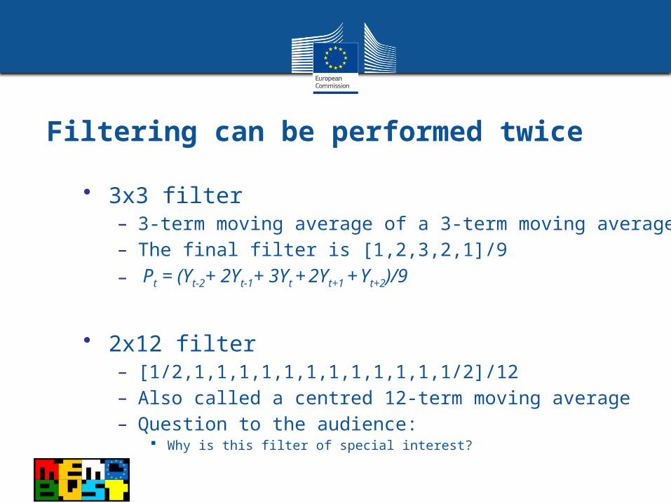
Filtering can be performed twice

• 3x3 filter– 3-term moving average of a 3-term moving average– The final filter is [1,2,3,2,1]/9– Pt = (Yt-2+ 2Yt-1+ 3Yt + 2Yt+1 + Yt+2)/9

• 2x12 filter– [1/2,1,1,1,1,1,1,1,1,1,1,1,1/2]/12– Also called a centred 12-term moving average– Question to the audience:

Why is this filter of special interest?

Henderson filters

• Finding filters with good properties is an interesting topic …

• Hederson (1916) introduces the so-called Henderson filters

• X-12-ARIMA uses this type of filter to calculate the trend

• The filter length determines the degree of smoothing

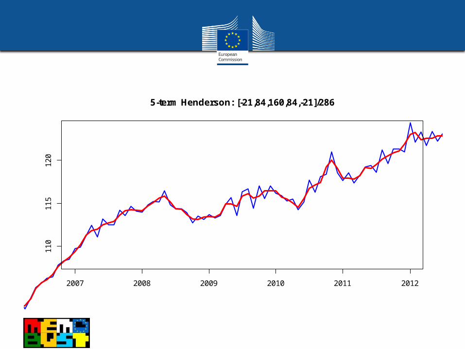
5-term Henderson: [-21,84,160,84,-21]/286

2007 2008 2009 2010 2011 2012

11

01

15

12

0

7-term Henderson: [-42,42,210,295,210,42,-42]/715

2007 2008 2009 2010 2011 2012

11

01

15

12

0

13-term Henderson: [-325,-468,0,1100,2475,3600,4032,3600,2475,1100,0,-468,-325]/16796

2007 2008 2009 2010 2011 2012

11

01

15

12

0

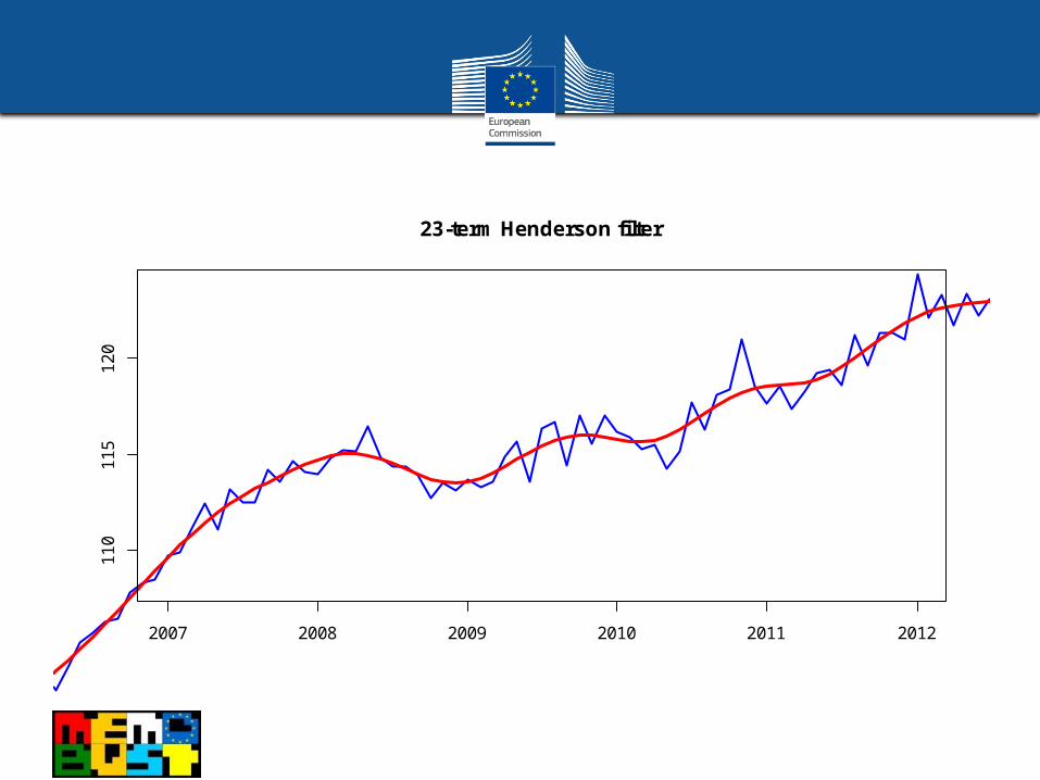
23-term Henderson filter

2007 2008 2009 2010 2011 2012

11

01

15

12

0

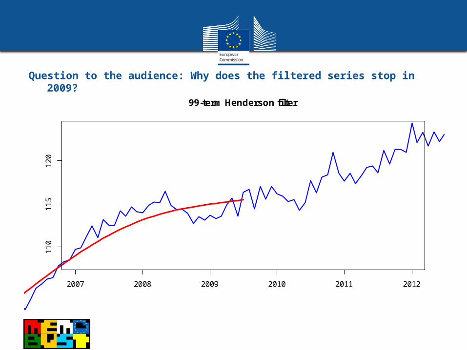
Question to the audience: Why does the filtered series stop in 2009?

99-term Henderson filter

2007 2008 2009 2010 2011 2012

11

01

15

12

0

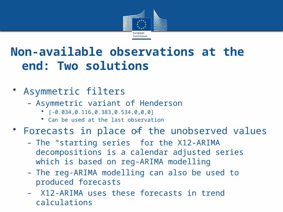
Non-available observations at the end: Two solutions

• Asymmetric filters– Asymmetric variant of Henderson

[-0.034,0.116,0.383,0.534,0,0,0] Can be used at the last observation

• Forecasts in place of the unobserved values – The “starting series” for the X12-ARIMA decompositions is

a calendar adjusted series which is based on reg-ARIMA modelling

– The reg-ARIMA modelling can also be used to produced forecasts

– X12-ARIMA uses these forecasts in trend calculations

Finding the seasonal component by filtering

• From a series with the trend removed we make 12 series– January-values, February-values, …

• Each of these series is smoothed by filtering • Altogether these smoothed series are the

seasonal component

Series with trend removed

2000 2002 2004 2006 2008 2010 2012 2014

0.9

1.0

1.1

1.2

1.3

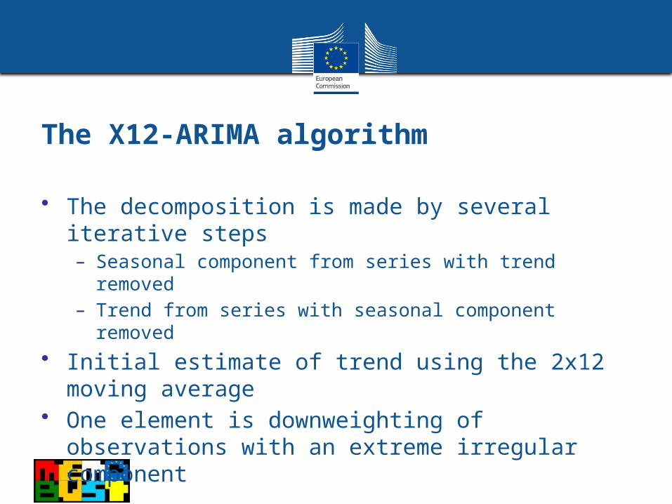
The X12-ARIMA algorithm

• The decomposition is made by several iterative steps– Seasonal component from series with trend removed– Trend from series with seasonal component removed

• Initial estimate of trend using the 2x12 moving average

• One element is downweighting of observations with an extreme irregular component

X12-ARIMA or SEATS

• Both method can be viewed as filtering techniques

• X12-ARIMA– A non-parametric method – No model assumed

• SEATS– The components are assumed to follow ARIMA models– The filters are derived from modelling – Possible to do inference and to make forecasts with

confidence intervals

– So why the name X12-ARIMA when this method is the one that is not based on ARIMA?

Answer on the next slide

Calendar adjustment by reg-ARIMA modelling

• Seasonal ARIMA model– Correlated errors (autocorrelation)– Differencing the series makes the model quite good without explicit

parameters for trend and seasonality – Need to decide the type of ARIMA model: ARIMA(p,d,q)(P,D,Q)

• Regression parameters in the model– Calendar effects: Trading day, Moving holyday, … – Outliers and level shifts

• Here y can be a log-transformed and leap-year adjusted variant of the original data

"The dirty model" mentioned earlier:

This slide is “stolen” from https://www.scss.tcd.ie/Rozenn.Dahyot/ST7005/15SeasonalARIMA.pdf

Here B is the backshift operator: BYt =Yt-1

ARIMA(0,1,1)(0,1,1)

Most common model

Airline model

Example of regression variables

in reg-ARIMA modelling

• Easter – 2000 and 2001: Easter in

April– 2008: Easter in March– 2002: 4 of 5 Norwegian

Easter days in March

• Trading day– Six parameters needed to

model seven days – Mon: Number of Mondays

minus Number of Sundays

Easter Mon Tue Wed Thu Fri SatJan 2000 0.0000000 0 -1 -1 -1 -1 0Feb 2000 0.0000000 0 1 0 0 0 0Mar 2000 -0.2571429 0 0 1 1 1 0Apr 2000 0.2571429 -1 -1 -1 -1 -1 0May 2000 0.0000000 1 1 1 0 0 0Jun 2000 0.0000000 0 0 0 1 1 0Jul 2000 0.0000000 0 -1 -1 -1 -1 0Aug 2000 0.0000000 0 1 1 1 0 0Sep 2000 0.0000000 0 0 0 0 1 1Oct 2000 0.0000000 0 0 -1 -1 -1 -1Nov 2000 0.0000000 0 0 1 1 0 0Dec 2000 0.0000000 -1 -1 -1 -1 0 0Jan 2001 0.0000000 1 1 1 0 0 0Feb 2001 0.0000000 0 0 0 0 0 0Mar 2001 -0.2571429 0 0 0 1 1 1Apr 2001 0.2571429 0 -1 -1 -1 -1 -1May 2001 0.0000000 0 1 1 1 0 0Jun 2001 0.0000000 0 0 0 0 1 1Jul 2001 0.0000000 0 0 -1 -1 -1 -1Aug 2001 0.0000000 0 0 1 1 1 0Sep 2001 0.0000000 -1 -1 -1 -1 -1 0Oct 2001 0.0000000 1 1 1 0 0 0Nov 2001 0.0000000 0 0 0 1 1 0Dec 2001 0.0000000 0 -1 -1 -1 -1 0Jan 2002 0.0000000 0 1 1 1 0 0Feb 2002 0.0000000 0 0 0 0 0 0Mar 2002 0.5428571 -1 -1 -1 -1 0 0Apr 2002 -0.5428571 1 1 0 0 0 0May 2002 0.0000000 0 0 1 1 1 0 : : :Mar 2008 0.7428571 0 -1 -1 -1 -1 0Apr 2008 -0.7428571 0 1 1 0 0 0May 2008 0.0000000 0 0 0 1 1 1Jun 2008 0.0000000 0 -1 -1 -1 -1 -1Jul 2008 0.0000000 0 1 1 1 0 0Aug 2008 0.0000000 -1 -1 -1 -1 0 0Sep 2008 0.0000000 1 1 0 0 0 0Oct 2008 0.0000000 0 0 1 1 1 0Nov 2008 0.0000000 -1 -1 -1 -1 -1 0Dec 2008 0.0000000 1 1 1 0 0 0

Trading day: Separate effect of each day or

common effect of all weekdays?

• Question to the audience:– Why exactly

equal t-values?

Regression Model -------------------------------------------------------------- Parameter Standard Variable Estimate Error t-value -------------------------------------------------------------- Trading Day Mon -0.0019 0.00193 -1.00 Tue 0.0064 0.00194 3.31 Wed 0.0018 0.00190 0.94 Thu -0.0016 0.00195 -0.81 Fri 0.0138 0.00188 7.37 Sat 0.0034 0.00193 1.73 *Sun (derived) -0.0219 0.00196 -11.16

Regression Model -------------------------------------------------------------- Parameter Standard Variable Estimate Error t-value -------------------------------------------------------------- Trading Day Weekday 0.0036 0.00053 6.87 **Sat/Sun (derived) -0.0090 0.00131 -6.87

Outliers

• An extreme observation caused by a special event can be problematic – Can influence the modelling in a negative way

Parameter estimates Forecasts Decomposition

• Solution – Include the outlier as a dummy variable in the reg-ARIMA

modelling ….0,0,0,0,0,0,0,0,0,1,0,0,0,0,0,0,0,0….

– The outlier is included in the irregular component after modelling

The observation is still included in seasonally adjusted data But has no effect on the trend

Question to the audience: Examples of special events?

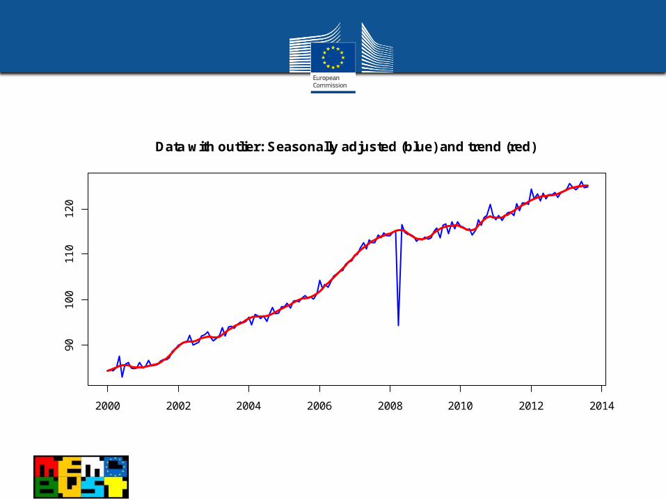
Data with outlier: Seasonally adjusted (blue) and trend (red)

2000 2002 2004 2006 2008 2010 2012 2014

90

10

01

10

12

0

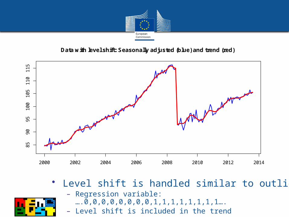
Data with level shift: Seasonally adjusted (blue) and trend (red)

2000 2002 2004 2006 2008 2010 2012 2014

85

90

95

10

01

05

11

01

15

• Level shift is handled similar to outliers– Regression variable: ….0,0,0,0,0,0,0,0,1,1,1,1,1,1,1,1…. – Level shift is included in the trend

Presented by

• László Sajtos

• Hungarian Central Statistical Office

Topics

• Seasonal adjustment step-by-step

• (A few) issues on seasonal adjustment

Seasonal adjustment step-by-step

Seasonal adjustment step-by-step: structure

Input data

STEPS with check points

Preliminary results

Output data

If results are acceptable

Not acceptable results

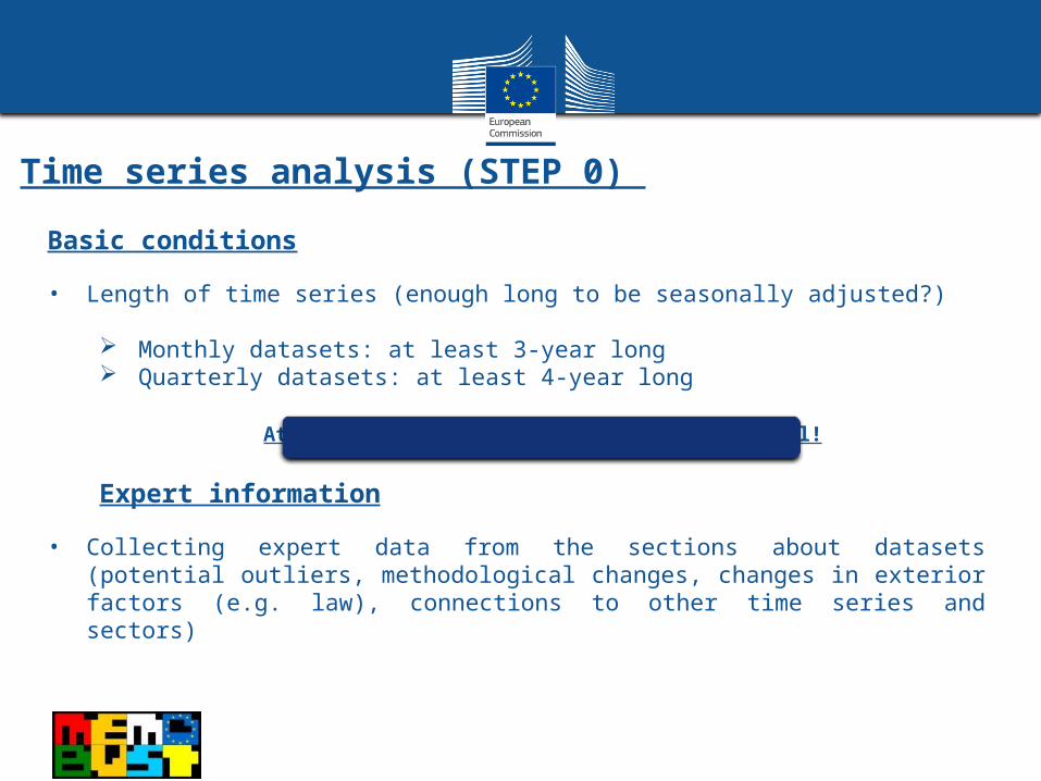
Basic conditions

• Length of time series (enough long to be seasonally adjusted?)

Monthly datasets: at least 3-year long Quarterly datasets: at least 4-year long

At least 5-7-year long time series is optimal!

Expert information

• Collecting expert data from the sections about datasets (potential outliers, methodological changes, changes in exterior factors (e.g. law), connections to other time series and sectors)

Time series analysis (STEP 0)

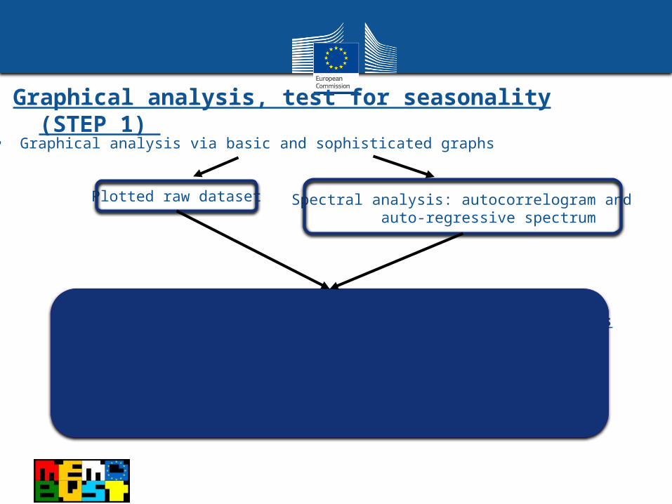
• Graphical analysis via basic and sophisticated graphs

Plotted raw dataset Spectral analysis: autocorrelogram and auto-regressive spectrum

• Identifying and explaining missing observations and outliers

• Correction of data faults

• Test for seasonality

Graphical analysis, test for seasonality (STEP 1)

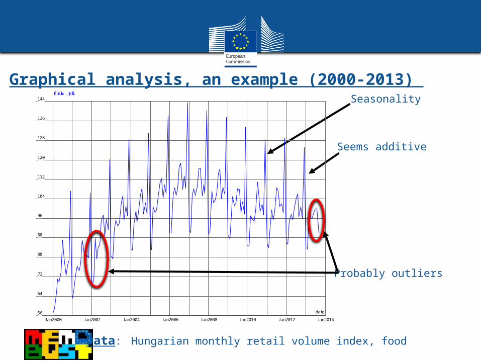
Seasonality

Seems additive

Data: Hungarian monthly retail volume index, food

date

J an2000 J an2002 J an2004 J an2006 J an2008 J an2010 J an2012 J an2014

56

64

72

80

88

96

104

112

120

128

136

144Élelm. jell.

Probably outliers

Graphical analysis, an example (2000-2013)

Automatic test

Graphical analysis

Software tools

Verification

Type of transformation (STEP 2)

Determining factors which may affect (regressors)+national holidays

Non-significance or absence Little significance

Keep

Sig

nifi

cance

Elimination

Consideration based on professional reasons

Consideration based on professional reasons

Elimination

Calendar adjustment (STEP 3)

Outlier treatment (Step 4)

Automatic outlier testing

Software tools

Verifying the results

STEP 1

Keep it

Significant

MonitoringStabilit

y

Available expert information

Less significant, but professionally

reasonable

Not significant

Eliminate it

Consideration based on professional reasons

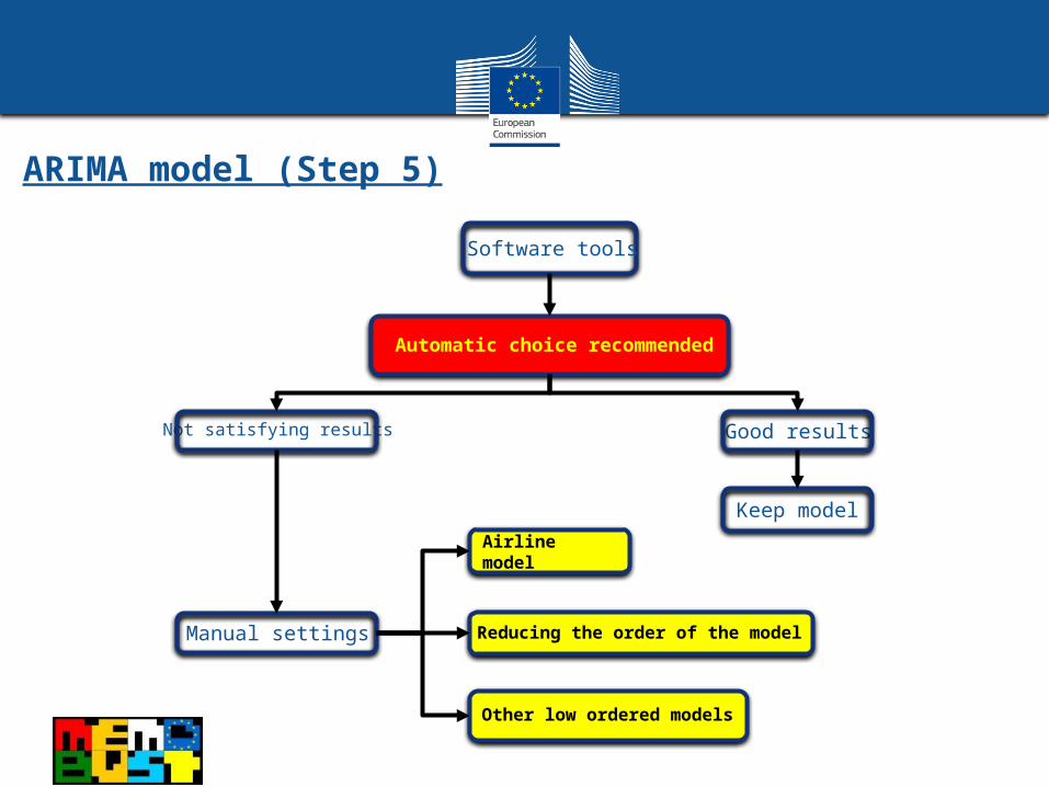
Airline model

Software tools

Not satisfying results Good results

Keep model

Manual settings

Automatic choice recommended

Other low ordered models

Reducing the order of the model

ARIMA model (Step 5)

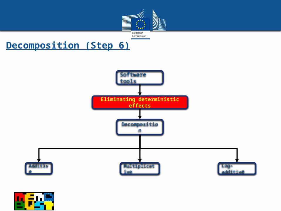
Decomposition (Step 6)

Software tools

Eliminating deterministic effects

Decomposition

Multiplicative Log-additiveAdditive

Quality diagnostics (Step 7)

1. Model adequacy on residuals:

• Ljung-Box test• Box-Pierce test

2. Seasonality: based on spectral graphics

3. Stability analysis: sliding spans

Documentation required!

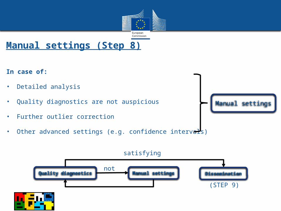
Manual settings (Step 8)

In case of:

• Detailed analysis

• Quality diagnostics are not auspicious

• Further outlier correction

• Other advanced settings (e.g. confidence intervals)

Manual settings

Quality diagnostics Dissemination

satisfying

Manual settingsnot

(STEP 9)

EXAMPLE (IN DEMETRA 2.04 SOFTWARE)

HUNGARIAN INDUSTRIAL TIME SERIES

Automated module

Open the input database

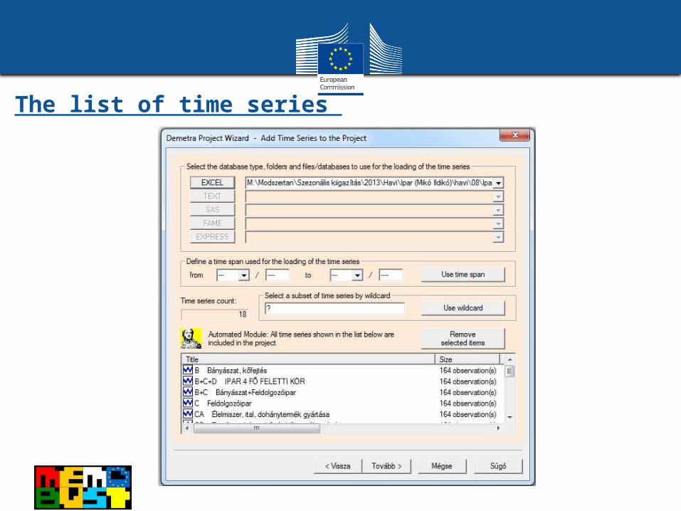
The list of time series

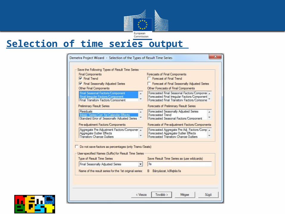
Selection of time series output

Save of output

Diagnostic, outlier %

Adjustment without fixed models

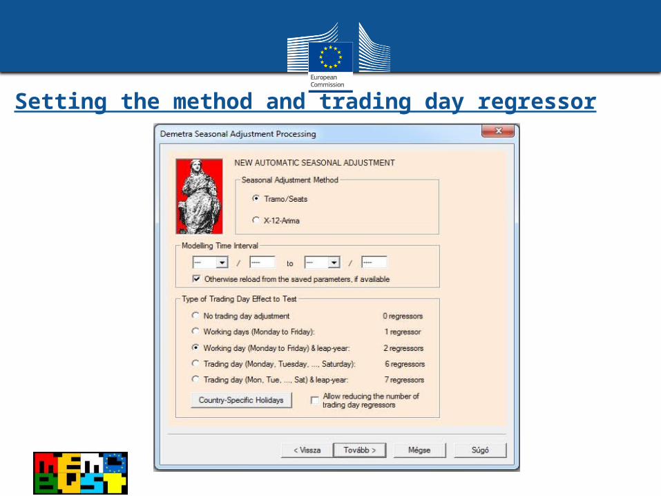
Setting the method and trading day regressor

Setting the country specific holidays

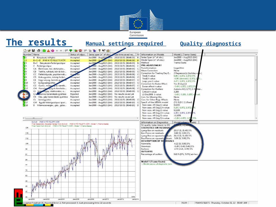
The results Manual settings required Quality diagnostics

(A few) issues on seasonal adjustment

Issues in Memobust book

• Consistency issues Data presentation

• Revision Issues on chained indices

• Treatment of the crisis Documentation

• Communication with users

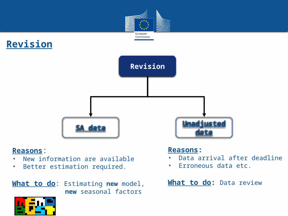
Revision

Revision

SA dataUnadjusted

data

Reasons:• Data arrival after deadline• Erroneous data etc.

What to do: Data review

Reasons:• New information are available• Better estimation required.

What to do: Estimating new model, new seasonal factors

Revision strategies

Goal: preserving accuracy, taking new information into consideration while

avoiding large changes reliability and stability

Strategies:

Extreme types Current Concurrent

Alternative types Partial concurrent

Controlled current

Extreme types

Alternative types

Horizon of revision

Practices:

• ESS Guideline: 3-4 years before the beginning of the revision period

• Statistics Denmark: at least 13 months back in time

Question: How many months of data should be revised?

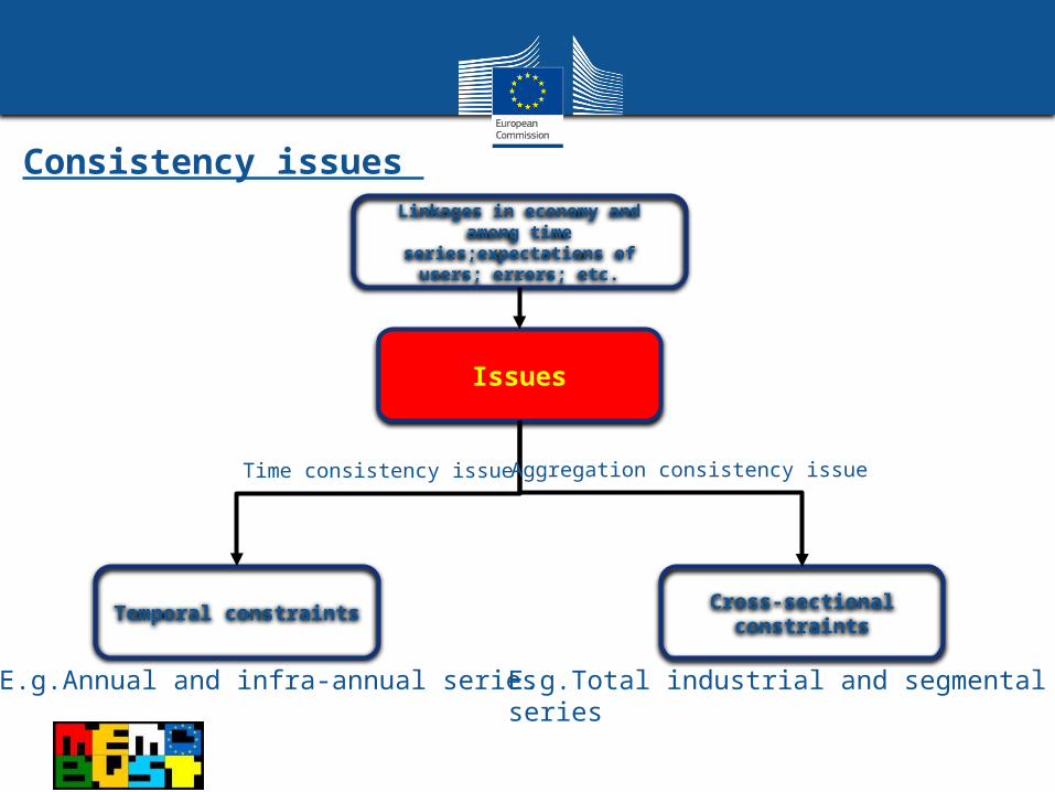
Consistency issues

Issues

Linkages in economy and among time

series;expectations of users; errors; etc.

Temporal constraints

E.g.Annual and infra-annual series

Cross-sectional constraints

E.g.Total industrial and segmental series

Time consistency issue Aggregation consistency issue

Time consistency issues

Problem: consistency of, for instance, sub-annual and annual series e.g. GDP

Sources of inconsistency:

• Less and more accurate data are compared;• Sampling errors;• Errors in evaluation

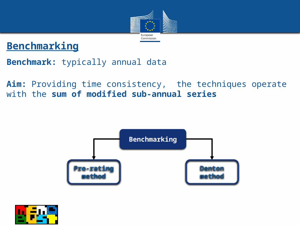
Benchmarking

Benchmark: typically annual data

Aim: Providing time consistency, the techniques operate with the sum of modified sub-annual series

Benchmarking

Pro-rating method

Denton method

Pro-rating method

How it works: multiplies the sub-annual values by the corresponding annual proportional discrepancies

Example: Three observations (), requirement:

Corrected values: ;

Denton method

How it works: Based on quadratic optimalization

Advantages:

• The method can be developed, specificated

• More reliable results (smaller discontinuities compared with pro-rating)

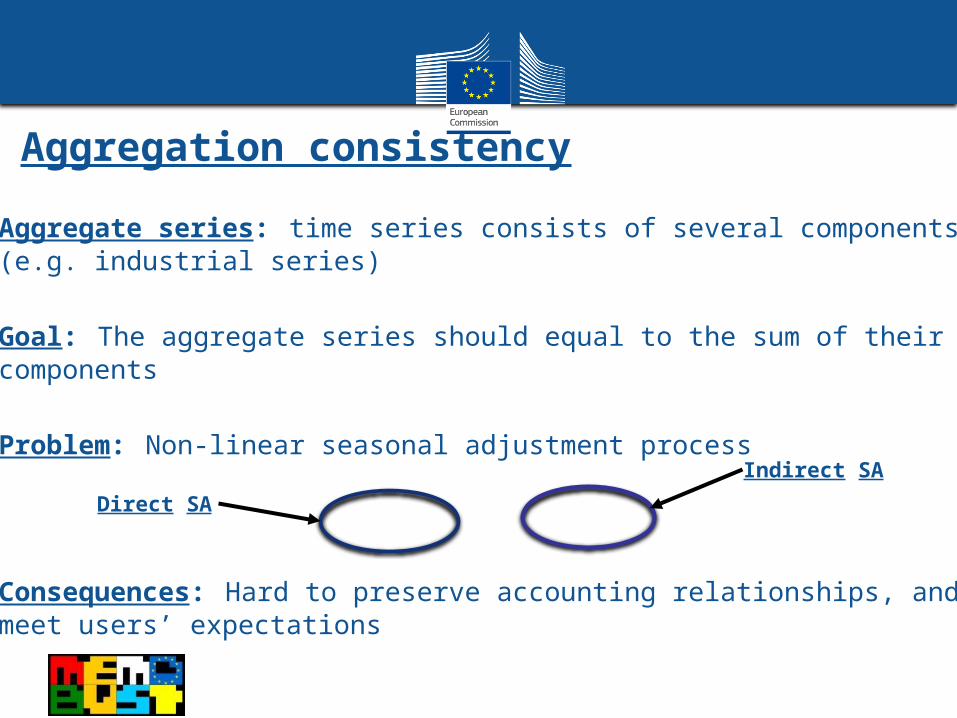
Aggregation consistency

Aggregate series: time series consists of several components (e.g. industrial series)

Goal: The aggregate series should equal to the sum of their components

Problem: Non-linear seasonal adjustment process

Consequences: Hard to preserve accounting relationships, and meet users’ expectations

Indirect SA

Direct SA

Methods to achieve aggregation consistency

• Only direct or indirect seasonal adjustment

• Pro-rating

• Denton method

• Regression based models

Thank you for your attention!

Questions?