ViEWS: A political Violence Early Warning System Journal...
43
Online Appendix for “ViEWS: A political Violence Early Warning System” Article published in Journal of Peace Research 56(2) (https://journals.sagepub.com/home/jpr) H˚ avard Hegre 1,3 , Marie Allansson 1 , Matthias Basedau 1,4 , Michael Colaresi 1,2 , Mihai Croicu 1 , Hanne Fjelde 1 , Frederick Hoyles 1 , Lisa Hultman 1 , Stina H¨ ogbladh 1 , Remco Jansen 1 , Naima Mouhleb 1 , Sayyed Auwn Muhammad 1 , Desir´ ee Nilsson 1 , H˚ avard Mokleiv Nyg˚ ard 1,3 , Gudlaug Olafsdottir 1 , Kristina Petrova 1 , David Randahl 1 , Espen Geelmuyden Rød 1 , Gerald Schneider 1,5 , Nina von Uexkull 1 , and Jonas Vestby 3 1 Department of Peace and Conflict Research, Uppsala University 2 University of Pittsburgh 3 Peace Research Institute Oslo 4 German Institute of Global and Area Studies 5 University of Konstanz February 14, 2019 Abstract This online appendix supports the article ‘ViEWS: A political Violence Early Warning System’ (Hegre et al., 2019), and further documents the ViEWS early-warning system. It details the various predic- tors used in ViEWS, defines the units of analysis in use, describes the statistical modeling, the use of downsampling, calibration, and ensemble modeling, and explain how missing and incomplete data were treated. The document continues to provide more details on the evaluation of the system, presents some additional forecasting results, and describes data management procedures in use. ViEWS PREDICTING CONFLICT Funding ViEWS receives funding from the European Research Council (ERC) under the European Union’s Horizon 2020 research and innovation programme (grant agreement no 694640) as well as from Uppsala Univer- sity. ViEWS computations are performed on resources provided by the Swedish National Infrastructure for Computing (SNIC) at Uppsala Multidisciplinary Center for Advanced Computational Science (UPPMAX). 1
Transcript of ViEWS: A political Violence Early Warning System Journal...

Online Appendix for
“ViEWS: A political Violence Early Warning System”
Article published in Journal of Peace Research 56(2)
(https://journals.sagepub.com/home/jpr)
Havard Hegre1,3, Marie Allansson1, Matthias Basedau1,4, Michael Colaresi1,2, Mihai Croicu1, HanneFjelde1, Frederick Hoyles1, Lisa Hultman1, Stina Hogbladh1, Remco Jansen1, Naima Mouhleb1,Sayyed Auwn Muhammad1, Desiree Nilsson1, Havard Mokleiv Nygard1,3, Gudlaug Olafsdottir1,
Kristina Petrova1, David Randahl1, Espen Geelmuyden Rød1, Gerald Schneider1,5, Nina vonUexkull1, and Jonas Vestby3
1Department of Peace and Conflict Research, Uppsala University2University of Pittsburgh
3Peace Research Institute Oslo4German Institute of Global and Area Studies
5University of Konstanz
February 14, 2019
Abstract
This online appendix supports the article ‘ViEWS: A political Violence Early Warning System’ (Hegreet al., 2019), and further documents the ViEWS early-warning system. It details the various predic-tors used in ViEWS, defines the units of analysis in use, describes the statistical modeling, the use ofdownsampling, calibration, and ensemble modeling, and explain how missing and incomplete data weretreated. The document continues to provide more details on the evaluation of the system, presents someadditional forecasting results, and describes data management procedures in use.
ViEWSPREDICTING CONFLICT
Funding
ViEWS receives funding from the European Research Council (ERC) under the European Union’s Horizon2020 research and innovation programme (grant agreement no 694640) as well as from Uppsala Univer-sity. ViEWS computations are performed on resources provided by the Swedish National Infrastructure forComputing (SNIC) at Uppsala Multidisciplinary Center for Advanced Computational Science (UPPMAX).
1

ViEWS February 14, 2019 Online appendix
Contents
A Predictors 3A.1 Country-level predictors . . . . . . . . . . . . . . . . . . . . . . . . . . . . . . . . . . . . . . . . . . . . 3
Baseline . . . . . . . . . . . . . . . . . . . . . . . . . . . . . . . . . . . . . . . . . . . . . . . . . . . . . 3Conflict history theme . . . . . . . . . . . . . . . . . . . . . . . . . . . . . . . . . . . . . . . . . . . . . 3Demography theme . . . . . . . . . . . . . . . . . . . . . . . . . . . . . . . . . . . . . . . . . . . . . . . 4Economy theme . . . . . . . . . . . . . . . . . . . . . . . . . . . . . . . . . . . . . . . . . . . . . . . . . 4Institutions theme . . . . . . . . . . . . . . . . . . . . . . . . . . . . . . . . . . . . . . . . . . . . . . . 5Protest theme . . . . . . . . . . . . . . . . . . . . . . . . . . . . . . . . . . . . . . . . . . . . . . . . . . 6
A.2 PRIO-GRID-level predictors . . . . . . . . . . . . . . . . . . . . . . . . . . . . . . . . . . . . . . . . . . 6Baseline . . . . . . . . . . . . . . . . . . . . . . . . . . . . . . . . . . . . . . . . . . . . . . . . . . . . . 6Conflict history theme . . . . . . . . . . . . . . . . . . . . . . . . . . . . . . . . . . . . . . . . . . . . . 6Natural geography theme . . . . . . . . . . . . . . . . . . . . . . . . . . . . . . . . . . . . . . . . . . . 8Social geography theme . . . . . . . . . . . . . . . . . . . . . . . . . . . . . . . . . . . . . . . . . . . . 9CM theme . . . . . . . . . . . . . . . . . . . . . . . . . . . . . . . . . . . . . . . . . . . . . . . . . . . . 9Protest theme . . . . . . . . . . . . . . . . . . . . . . . . . . . . . . . . . . . . . . . . . . . . . . . . . . 11
B Levels of analysis and dependent variables 12B.1 Levels of analysis . . . . . . . . . . . . . . . . . . . . . . . . . . . . . . . . . . . . . . . . . . . . . . . . 12B.2 The dependent variable: recent history . . . . . . . . . . . . . . . . . . . . . . . . . . . . . . . . . . . . 12B.3 The persistence of conflict in Africa . . . . . . . . . . . . . . . . . . . . . . . . . . . . . . . . . . . . . . 14B.4 Descriptive statistics . . . . . . . . . . . . . . . . . . . . . . . . . . . . . . . . . . . . . . . . . . . . . . 15
C Statistical modeling 15C.1 Estimation of constituent models . . . . . . . . . . . . . . . . . . . . . . . . . . . . . . . . . . . . . . . 15
D Ensemble Bayesian Model Averaging 15D.1 Combining three types of political violence outcomes . . . . . . . . . . . . . . . . . . . . . . . . . . . . 16
E Downsampling and calibration 16E.1 Downsampling . . . . . . . . . . . . . . . . . . . . . . . . . . . . . . . . . . . . . . . . . . . . . . . . . 16E.2 Calibration . . . . . . . . . . . . . . . . . . . . . . . . . . . . . . . . . . . . . . . . . . . . . . . . . . . 17
F Handling missing or incomplete data in ViEWS 18F.1 Dependent variables . . . . . . . . . . . . . . . . . . . . . . . . . . . . . . . . . . . . . . . . . . . . . . 18F.2 Predictors . . . . . . . . . . . . . . . . . . . . . . . . . . . . . . . . . . . . . . . . . . . . . . . . . . . . 19
G Detailed evaluation, state-based conflict (sb) 19G.1 AUROC, Brier, and AUPR, cm level . . . . . . . . . . . . . . . . . . . . . . . . . . . . . . . . . . . . . 21
Bi-separation plots, cm level . . . . . . . . . . . . . . . . . . . . . . . . . . . . . . . . . . . . . . . . . . 22Confusion matrices, cm level . . . . . . . . . . . . . . . . . . . . . . . . . . . . . . . . . . . . . . . . . 23
G.2 AUROC, Brier, and AUPR, pgm level . . . . . . . . . . . . . . . . . . . . . . . . . . . . . . . . . . . . 24Confusion matrices, pgm level . . . . . . . . . . . . . . . . . . . . . . . . . . . . . . . . . . . . . . . . . 25
H Evaluation, ns 29
I Evaluation, os 32
J Additional forecasting results 35
K Data management 40
L Future extensions 40
2

ViEWS February 14, 2019 Online appendix
A Predictors
Here, we present all the predictors used in ViEWS, organized by the themes presented in Tables 2 and3 in the main paper. We state the name the variables have in the database, report the sources for theinformation, and summarize how we have processed the data.
A.1 Country-level predictors
The country-level (cm) predictors are organized in six themes as detailed in Table 2 in the main paper.
Baseline
For each dependent variable the baseline model is the country-level mean of the dependent variable itself inthe training period. This model is intuitively similar to a model with only individual fixed effects and noother predictors but easier for us to estimate.
Mean of state based conflict computed for the training period (mean ged dummy sb) Country-level mean of the incidence of state based violence computed for the training period.
Mean of non-state conflict computed for the training period (mean ged dummy ns) Country-levelmean of the incidence of non-state conflict computed for the training period.
Mean of one sided violence computed for the training period (mean ged dummy os) Country-levelmean of the incidence of one sided violence computed for the training period.
Mean of protest incidence computed for the training period (mean acled dummy pr) Country-level mean of the incidence of protests computed for the training period.
Conflict history theme
Conflict history models for each of the outcomes includes all decay functions of time since conflict events,the first order temporal lag of all outcomes and all temporal lags from 1 to 12 months of the dependentvariable itself.
Decay function of time since state-based conflict event (decay 12 cw ged dummy sb 0) Exponentialdecay function applied to months since state-based conflict in the country. The decay function is
2−tse12
where tse is time since event in months. It has a half-life of 12 months.
Decay function of time since non-state conflict event (decay 12 cw ged dummy ns 0) Exponential12-month half-life decay function applied to months since non-state conflict in the country.
Decay function of time since one-sided violence event (decay 12 cw ged dummy os 0) Exponential12-month half-life decay function applied to months since one-sided violence in the country.
Lagged state-based conflict event (li ged dummy sb). Lagged state-based conflict in the country. 1 ifconflict occurred i months ago, zero otherwise. Computed for each i ∈ (1, 2, .., 12)
Lagged non-state conflict event (li ged dummy ns). Lagged non-state conflict in the country. 1 ifconflict occurred i months ago, zero otherwise. Computed for each i ∈ (1, 2, .., 12)
3
ViEWS February 14, 2019 Online appendix
Lagged one-sided violence event (li ged dummy os). Lagged one-sided violence in the country. 1 ifconflict occurred i months ago, zero otherwise. Computed for each i ∈ (1, 2, .., 12)
Demography theme
Population size (ln fvp population200) The total population of a given country. This variable useshistorical data stitched together in order to gather information from 1900 until today, and continuing withprojections into the future. The variable is constructed with data from Maddison (2007), World Bank(2017) and Samir & Lutz (2008). First, we harmonize candidate data to the WDI series. We then assemblea time-series based on the following preference: WDI > Maddison WP-4. Third, the SSP projection (secondscenario ‘Middle of the Road’) is added for the future projections. Lastly, we interpolate the logged data inorder to remove missing values where this is possible. In order to have a gradual transition from one seriesto another we calculate a gradual exchange between the WDI value and the SSP value from 2007 until 2017.This variable is included in the natural logarithm form.
Proportion of population between 15 and 24 with at least lower secondary education (ssp2 edu sec 15 24 prop)The proportion of the population between 15 and 24 that has completed at least lower secondary schoolingimplies those that have completed lower or upper secondary school. Those that have attained tertiary edu-cation are included in this number. This variable is constructed using Samir & Lutz (2008) historical datafrom IIASA.
Proportion of population living in urban areas (ssp2 urban share iiasa) The proportion of thetotal population living in an urban area. This variable is taken from Samir & Lutz (2008) IIASA data,using historical data collected by the UN.
Economy theme
GDP per capita (fvp lngdppercapita200) The natural log of GDP per capita in a given country-year.This variable uses historical data stitched together in order to gather information from 1900 until today, andcontinuing with projections into the future. The variable is constructed with data from Maddison (2007),World Bank (2017) and Samir & Lutz (2008). In order to be able to put the data together into a serieswe needed to create divisors in order to convert them all into purchasing power parity adjusted 2005 USdollars. First, we harmonize all candidate data to the WDI2005PPP (NY.GDP.MKTP.PP.KD) series (wewant our measurement in 2005PPP units). We here assume that the ratio between the candidate dataand WDI2005PPP series is constant over time within a country. We then assemble a time-series basedon the following preference: WDI2005PPP > WDI2005 Constant US > Maddison WP-4. This preferenceis based on looking at the data and finding the series that fit best with the WDI data. Third, the SSPprojection (second scenario ‘Middle of the Road’) is added for the future projections. Lastly, we interpolatethe log(gdp/cap) data in order to remove missing values where this is possible.
Log GDP per capita, oilrents only (fvp lngdpcap oilrent) The natural log of GDP per capita fromoilrents in a given country-year. It is calculated using the World Bank Development indicator named ”Oilrents” (NY.GDP.PETR.RT.ZS) (World Bank, 2017), our GDP per capita measure and the population datanoted below. For the projections into the future we calculate the average percentage of GDP per capitaconstituted by oil rents for each country over the last five years of data and assume that the same rate willcontinue into the future.
Log GDP per capita, excluding oilrents (fvp lngdpcap nonoilrent) The natural log of GDP percapita excluding oilrents in a given country-year. Computed using the same methodology as Log GDP percapita including oilrents.
4

ViEWS February 14, 2019 Online appendix
Growth in Log GDP per capita, oilrents only (fvp grlngdpcap oilrent) Yearly change in thenatural log GDP per capita from oilrent sources in a given country-year. Growth computed as xt − xt−1.
Growth in Log GDP per capita, excluding oilrents (fvp grlngdpcap nonoilrent) Yearly changein natural log of GDP per capita excluding oilrents in a given country-year. Growth computed as xt−xt−1.
Institutions theme
Democracy index (fvp democracy) This index uses three dimensions from V-Dem 7.1 Coppedge et al.(2017) to classify the level of democracy in each country. These dimensions are centered on: free and fair elec-tions (v2x polyarchy), democratic participation (v2x partip) and constraints on the executive (v2x liberal).The higher the performance on any or each of these leads to a higher score on the democracy index, andvice versa. The variable ranges from 0 to one, where one is the highest possible level of democracy.
Democracy (fvp demo) This variable is a dummy variable, indicating whether or not this country is tobe regarded a democracy or not. If it does fall into the definition of democracy it is coded one, if not, it iscoded 0. This classification is constructed on the basis of the Democracy index variable. To construct thecategories we rely on a cube produced by plotting the three dimensions against each other. We calculate theEuclidean distance from the democracy and autocracy corners and standardize the distance to fall between0 and 1. We then define as a democracy any country-year that is no further from the democracy corner than0.40, and as autocratic any country that is less than 0.40 from the autocracy corner. The semi-democracies,thus, are those that are in between.
Semi-democracy (fvp semi) This variable is a dummy variable, indicating whether or not this countryis to be regarded a semi-democracy or not. If it does fall into the definition of semi-democracy it is codedone, if not, it is coded 0. This classification is constructed on the basis of the Democracy index variable. Toconstruct the categories we rely on a cube produced by plotting the three dimensions against each other. Wecalculate the Euclidean distance from the democracy and autocracy corners and standardize the distanceto fall between 0 and 1. We then define as a democracy any country-year that is no further from thedemocracy corner than 0.40, and as autocratic any country that is less than 0.40 from the autocracy corner.The semi-democracies, thus, are those that are in between.
Autocracy (fvp auto) This variable is a dummy variable, indicating whether or not this country is tobe regarded an autocracy or not. If it does fall into the definition of autocracy it is coded one, if not, it iscoded 0. This classification is constructed on the basis of the Democracy index variable. To construct thecategories we rely on a cube produced by plotting the three dimensions against each other. We calculate theEuclidean distance from the democracy and autocracy corners and standardize the distance to fall between0 and 1. We then define as a democracy any country-year that is no further from the democracy corner than0.40, and as autocratic any country that is less than 0.40 from the autocracy corner. The semi-democracies,thus, are those that are in between.
Time since pre-independence war (ln fvp timesincepreindepwar) The total number of years sincethe country experienced a pre-independence war. This is based on the entrance dates set by Gleditsch &Ward (1999). Included in natural logarithm form.
Time since regime change (ln fvp timesinceregimechange) The total number of years since thecountry experienced regime change. Defined by changes between the dummy variables fvp demo, fvp semiand fvp auto. Included in natural logarithm form.
5

ViEWS February 14, 2019 Online appendix
Proportion of population excluded from power (fvp prop excluded) Number of excluded ethnicgroups (discriminated or powerless) in the country for a given year. Derived from the EPR 2014 update2 dataset (Vogt et al., 2015). Missing data is filled in through linear interpolations. This is used forcountry-level using EPR’s non-georeferenced data.
Time since independence (ln fvp timeindep) The total number of years since the country becamean internationally recognized sovereign state. This is based on the entrance dates set by Gleditsch & Ward(1999). Included in natural logarithm form.
Protest theme
Decay function of time since protest event (decay 12 cw acled dummy pr 0) Exponential 12-monthhalf-life decay function applied to months since non-state conflict in the same country. The decay functionis
2−tse12
where tse is time since event in months. It has a half-life of 12 months.
Lagged protest event (li acled dummy pr). Lagged ACLED protest events in the country. 1 if conflictoccurred i months ago, zero otherwise. Computed for each i ∈ (1, 2, .., 12)
A.2 PRIO-GRID-level predictors
The PRIOGRID-level (pgm) predictors are organized in six themes as detailed in Table 3 in the main paper.
Baseline
For each dependent variable the baseline model is the country-level mean of the dependent variable itself inthe training period. This model is intuitively similar to a model with only individual fixed effects and noother predictors but easier for us to estimate.
Mean of state based conflict computed for the training period (mean ged dummy sb) Grid-cellmean of the incidence of state based violence computed for the training period.
Mean of non-state conflict computed for the training period (mean ged dummy ns) Grid-cellmean of the incidence of non-state conflict computed for the training period.
Mean of one sided violence computed for the training period (mean ged dummy os) Grid-cellmean of the incidence of one sided violence computed for the training period.
Mean of protest incidence computed for the training period (mean acled dummy pr) Grid-cellmean of the incidence of protests computed for the training period.
Conflict history theme
For each dependent variable’s model the conflict history theme includes:
• Decay function of time since all outcomes.
• First order temporal lags of all other outcomes.
• First to twelth order temporal lag of the dependent variable.
6

ViEWS February 14, 2019 Online appendix
• First order spatial lag of first order temporal lag of all other outcomes.
• First order spatial lag of first, second and third order temporal lag of dependent variable.
State based conflict event (ged dummy sb) Dummy variable indicating whether there was a conflictevent (at least one battle related death) in a given grid cell in a given month. State based conflicts, thatis intra-state, inter-state, internationalized and extrasystemic conflicts (Sundberg & Melander, 2013). Inthe country models this is aggregated up to the country level using cShapes v.0.4-2. (Weidmann, Kuse& Gleditsch, 2010). Included in various transformations as a predictor and as the dependent variable formodels of state based conflict.
Non-state conflict event (ged dummy ns) Dummy variable indicating whether a non-state conflictevent (at least one battle related death) had occurred within the given grid cell. Non-state conflicts, wherenon-state armed groups are in conflict with one another (Sundberg & Melander, 2013). Included in varioustransformations as a predictor and as the dependent variable for models of non-state conflict.
One-sided conflict event (ged dummy os) Dummy variable indicating whether there was a conflictevent (at least one death) in a given grid cell in a given month. One-sided violence regards cases wheregovernment forces or non-state armed groups engage in violence against civilians (Sundberg & Melander,2013). Included in various transformations as a predictor and as the dependent variable for models ofone-sided violence.
Lagged state-based conflict event (li ged dummy sb) Lagged state-based conflict in the grid cell.1 if conflict occurred i months ago, 0 otherwise. Computed for each i ∈ (1, 2, .., 12)
Lagged non-state conflict event (li ged dummy ns) Lagged non-state conflict in the grid cell. 1 ifconflict occurred i months ago, 0 otherwise. Computed for each i ∈ (1, 2, .., 12)
Lagged one-sided violence event (li ged dummy os) Lagged one-sided violence in the grid cell. 1 ifconflict occurred i months ago, 0 otherwise. Computed for each i ∈ (1, 2, .., 12)
Decay function of time since state-based conflict event (decay 12 cw ged dummy sb 0) Exponentialdecay function applied to months since state-based conflict in the same grid cell. The decay function is
2−tse12
where tse is time since event in months. It has a half-life of 12 months.
Decay function of time since non-state conflict event (decay 12 cw ged dummy ns 0) Exponential12-month half-life decay function applied to months since non-state conflict in the same grid cell.
Decay function of time since one-sided violence event (decay 12 cw ged dummy os 0) Exponential12-month half-life decay function applied to months since non-state conflict in the same grid cell.
Spatial lag of state-based conflict event (q 1 1 lt ged dummy sb). Sum of t month time-lagged state-based conflict events in the neighbouring grid cells. Neighbouring is defined by a queens movement in chessmeaning cells horizontally, vertically or diagonally adjacent. Computed for first order neighbors, meaningonly directly adjacent cells are considered. Computed for t ∈ (1, 2, 3). If all neighbouring cell had state-based conflict events one month ago q 1 1 l1 ged dummy sb takes the value 8. If only one neighbouring cellhad state-based conflict q 1 1 l1 ged dummy sb takes the value 1.
7

ViEWS February 14, 2019 Online appendix
Spatial lag of non-state conflict event (q 1 1 lt ged dummy ns). Sum of t month time-lagged non-state conflict events in the neighbouring grid cells. Neighbouring is defined by a queens movement in chessmeaning cells horizontally, vertically or diagonally adjacent. Computed for first order neighbors, meaningonly directly adjacent cells are considered. Computed for t ∈ (1, 2, 3).
Spatial lag of one-sided conflict event (q 1 1 lt ged dummy os). Sum of t month time-lagged one-sidede violence events in the neighbouring grid cells. Neighbouring is defined by a queens movement in chessmeaning cells horizontally, vertically or diagonally adjacent. Computed for first order neighbors, meaningonly directly adjacent cells are considered. Computed for t ∈ (1, 2, 3).
Natural geography theme
Distance to nearest secondary diamonds resource (ln dist diamsec). Captures the distance fromthe grid cell to the nearest secondary diamonds resource (static data). The distance is measured in loggedWGS86 units (decimal degrees), a unit closely resembling the design choices for the overall grid. The originalvariable is named diamsec s and is collected from PRIO-GRID, based on Klein Goldewijk et al. (2011).
Distance to nearest petroleum resource (ln dist petroleum). Captures the distance from the gridcell to the nearest petroleum resource (static data, and only onshore production). The distance is measuredin logged WGS86 units (decimal degrees), a unit closely resembling the design choices for the overall grid.The original variable is named petroleum s and is collected from PRIO-GRID, based on Klein Goldewijket al. (2011)
Proportion of mountainous terrain (mountain ih li). Percentage area of the cell covered by moun-tains. Collected from PRIO-GRID, based on ISAM-HYDE landuse data (Meiyappan & Jain, 2012). Missingdata is filled in through linear interpolation.
Agricultural area (agri ih li). Percentage area of the cell covered by agricultural area. Collectedfrom PRIO-GRID, based on ISAM-HYDE landuse data(Meiyappan & Jain, 2012). Missing data is filled inthrough linear interpolation.
Barren area (barren ih li). Percentage area of the cell covered by barren area. Collected from PRIO-GRID, based on ISAM-HYDE landuse data (Meiyappan & Jain, 2012). Missing data is filled in throughlinear interpolation.
Forest area (forest ih li). Percentage area of the cell covered by forest area. Collected from PRIO-GRID, based on ISAM-HYDE landuse data (Meiyappan & Jain, 2012). Missing data is filled in throughlinear interpolation.
Grasslands (savanna ih li). Percentage area of the cell covered by grasslands. Collected from PRIO-GRID, based on ISAM-HYDE landuse data (Meiyappan & Jain, 2012). Missing data is filled in throughlinear interpolation.
Shrublands (shrub ih li). Percentage area of the cell covered by shrublands. Collected from PRIO-GRID, based on ISAM-HYDE landuse data (Meiyappan & Jain, 2012). Missing data is filled in throughlinear interpolation.
Pasture land (pasture ih li). Percentage area of the cell covered by pasture area, based on ISAM-HYDE land-use data. In PRIO-GRID, this indicator is available for the years 1950, 1960, 1970, 1980, 1990,2000, and 2010 (Meiyappan & Jain, 2012). Missing data is filled in through linear interpolation.
8

ViEWS February 14, 2019 Online appendix
Social geography theme
Distance to neighboring country (ln bdist1). The spherical distance in kilometer from the cell cen-troid to the border of the nearest land-contiguous neighboring country, based on country border data usingcShapes v.0.4-2. (Weidmann, Kuse & Gleditsch, 2010). Included in natural logarithm form of the originalvariable.
Travel time (ln ttime). Log-transformed estimate of the travel time to the nearest major city, derivedfrom a global high-resolution raster map of accessibility developed for the EU (Uchida, 2009). Collectedfrom PRIO-GRID. Included in natural logarithm form of the original variable.
Distance to capital city (ln capdist). The spherical distance in kilometers from the cell centroid tothe national capital city in the corresponding country, based on coordinate pairs of capital cities derivedfrom the cShapes dataset v.0.4-2. It captures changes over time wherever relevant (Weidmann, Kuse &Gleditsch, 2010). Included in natural logarithm form of the original variable.
Population size (ln pop). Population size for each populated cell in the grid, taken from the HistoryDatabase of the Global Environment (HYDE) version 3.1. Population estimates are available for 1950,1960, 1970, 1980, 1990, 2000, and 2005. The original pixel value is number of persons. Included in naturallogarithm form of the original variable. Collected from PRIO-GRID, based on Klein Goldewijk et al. (2011).
Gross cell product (gcp li mer). The gross cell product, measured in USD, based on the G-Econdataset v4.0, last modified May 2011. The original G-Econ data represent the total economic activity at a1x1 degree resolution, so when assigning this to PRIO-GRID we distribute the total value across the numberof contained PRIO-GRID land cells. In border areas, the G-Econ 1x1 degree cells might overlap with PRIO-GRID cells allocated to a neighboring country.To minimize bias, PRIO-GRID only extracts G-Econ datafor cells that have the same country code as the G-Econ cell represents. This variable is only available forfive-year intervals since 1990 (Nordhaus, 2006). Missing data is filled in through linear interpolations.
Infant mortality rate(imr mean). Mean infant mortality rate. Collected from PRIO-GRID, based onraster data from the SEDAC Global Poverty Mapping project (Storeygard et al., 2008).
Proportion of mountainous terrain (mountains mean). Proportion of mountainous terrain withinthe cell based on elevation, slope and local elevation range. Collected from PRIO-GRID, taken from ahigh-resolution mountain raster developed for UNEPs Mountain Watch Report. (Blyth, 2002).
Urban area (urban ih li). Percentage area of the cell covered by urban area. Collected from PRIO-GRID, based on ISAM-HYDE landuse data(Meiyappan & Jain, 2012). Missing data is filled in throughlinear interpolations.
Excluded groups (excluded li). Number of excluded ethnic groups (discriminated or powerless) in thegrid cell for the given year. Collected from PRIO-GRID, derived from the GeoEPR 2014 update 2 dataset(Vogt et al., 2015). Missing data is filled in through linear interpolations. This is used for country-levelusing EPR’s non-georeferenced data.
CM theme
Democracy (fvp demo) This variable is a dummy variable, indicating whether or not this country is tobe regarded a democracy or not. If it does fall into the definition of democracy it is coded one, if not, it iscoded 0. This classification is constructed on the basis of A.1. To construct the categories we rely on a cubeproduced by plotting the three dimensions against each other. We calculate the Euclidean distance from
9

ViEWS February 14, 2019 Online appendix
the democracy and autocracy corners and standardize the distance to fall between 0 and 1. We then defineas a democracy any country-year that is no further from the democracy corner than 0.40, and as autocraticany country that is less than 0.40 from the autocracy corner. The semi-democracies, thus, are those thatare in between.
Semi-democracy (fvp semi) This variable is a dummy variable, indicating whether or not this countryis to be regarded a semi-democracy or not. If it does fall into the definition of semi-democracy it is codedone, if not, it is coded 0. This classification is constructed on the basis of A.1. To construct the categorieswe rely on a cube produced by plotting the three dimensions against each other. We calculate the Euclideandistance from the democracy and autocracy corners and standardize the distance to fall between 0 and 1.We then define as a democracy any country-year that is no further from the democracy corner than 0.40,and as autocratic any country that is less than 0.40 from the autocracy corner. The semi-democracies, thus,are those that are in between.
Time since pre-independence war (ln fvp timesincepreindepwar) The total number of years sincethe country experienced a pre-independence war. This is based on the entrance dates set by Gleditsch &Ward (1999). Included in natural logarithm form.
Time since regime change (ln fvp timesinceregimechange) The total number of years since thecountry experienced regime change. Defined by changes between the dummy variables fvp demo, fvp semiand fvp auto. Included in natural logarithm form.
Proportion of population excluded from power (fvp prop excluded) Number of excluded ethnicgroups (discriminated or powerless) in the country for a given year. Derived from the EPR 2014 update2 dataset (Vogt et al., 2015). Missing data is filled in through linear interpolations. This is used forcountry-level using EPR’s non-georeferenced data.
Time since independence (ln fvp timeindep) The total number of years since the country becamean internationally recognized sovereign state. This is based on the entrance dates set by Gleditsch & Ward(1999). Included in natural logarithm form.
GDP per capita (lnGDPpc200) The GDP per capita in a given country-year. This variable uses historicaldata stitched together in order to gather information from 1900 until today, and continuing with projectionsinto the future. The variable is constructed with data from Maddison (2007), World Bank (2017) and Samir& Lutz (2008). In order to be able to put the data together into a series we needed to create divisorsin order to convert them all into purchasing power parity adjusted 2005 US dollars. First, we harmonizeall candidate data to the WDI2005PPP (NY.GDP.MKTP.PP.KD) series (we want our measurement in2005PPP units). We here assume that the ratio between the candidate data and WDI2005PPP series isconstant over time within a country. We then assemble a time-series based on the following preference:WDI2005PPP > WDI2005ConstantUS > MaddisonWP − 4. This preference is based on looking at thedata and finding the series that fit best with the WDI data. Third, the SSP projection (second scenario‘Middle of the Road’) is added for the future projections. Lastly, we interpolate the log(gdp/cap) data inorder to remove missing values where this is possible. This variable is coded in the natural logarithm formof the original variable, and serves as a base for calculating the oil, and non-oil GDP per capita for eachcountry.
Log GDP per capita, oilrents only (fvp lngdpcap oilrent) The natural log of GDP per capita fromoilrents in a given country-year. It is calculated using the World Bank Development indicator named ”Oilrents” (NY.GDP.PETR.RT.ZS) (World Bank, 2017), our GDP per capita measure and the population datanoted below. For the projections into the future we calculate the average percentage of GDP per capita
10

ViEWS February 14, 2019 Online appendix
constituted by oil rents for each country over the last five years of data and assume that the same rate willcontinue into the future.
Log GDP per capita, excluding oilrents (fvp lngdpcap nonoilrent) The natural log of GDP percapita excluding oilrents in a given country-year. Computed using the same methodology as Log GDP percapita including oilrents.
Growth in Log GDP per capita, oilrents only (fvp grlngdpcap oilrent) Yearly change in thenatural log GDP per capita from oilrent sources in a given country-year. Growth computed as xt − xt−1.
Growth in Log GDP per capita, excluding oilrents (fvp grlngdpcap nonoilrent) Yearly changein natural log of GDP per capita excluding oilrents in a given country-year. Growth computed as xt−xt−1.
Population size (ln fvp population200) The total population of a given country. This variable useshistorical data stitched together in order to gather information from 1900 until today, and continuing withprojections into the future. The variable is constructed with data from Maddison (2007), World Bank (2017)and Samir & Lutz (2008). First, we harmonize candidate data to the WDI series (we want our measurementin thousands). We then assemble a time-series based on the following preference: WDI > MaddisonWP−4.Third, the SSP projection (second scenario ‘Middle of the Road’) is added for the future projections. Lastly,we interpolate the logged data in order to remove missing values where this is possible. In order to have agradual transition from one series to another we calculate a gradual exchange between the WDI value andthe SSP value from 2007 until 2017. This variable is included in the natural logarithm form of the originalvariable.
Proportion of population between 15 and 24 with at least lower secondary education (ssp2 edu sec 15 24 prop)The proportion of the population between 15 and 24 that has completed at least lower secondary schoolingimplies those that have completed lower or upper secondary school. Those that have attained tertiary edu-cation are included in this number. This variable is constructed using Samir & Lutz (2008) historical datafrom IIASA.
Proportion of population living in urban areas (ssp2 urban share iiasa) The proportion of thetotal population living in an urban area. This variable is taken from Samir & Lutz (2008) IIASA data,using historical data collected by the UN.
Protest theme
Protest event (acled dummy pr). Dummy variable indicating whether there was a protest event as de-fined by ACLED (Armed Conflict Location and Event Dataset) in a given grid cell in a given month (Raleighet al., 2010). Included in various transformations as a predictor and as the dependent variable for models ofprotest event incidence. Models of protest are used as auxilliary models in our dynamic simulation forecasts.
Decay function of time since protest event (decay 12 cw acled dummy pr 0) Exponential 12-monthhalf-life decay function applied to months since non-state conflict in the same country. The decay functionis
2−tse12
where tse is time since event in months. It has a half-life of 12 months.
Lagged protest event (li acled dummy pr). Lagged ACLED protest events in the country. 1 if conflictoccurred i months ago, zero otherwise. Computed for each i ∈ (1, 2, .., 12)
11

ViEWS February 14, 2019 Online appendix
Spatial lag of protest event (q 1 1 lt acled dummy pr). Sum of t month time-lagged state-based con-flict events in the neighbouring grid cells. Neighbouring is defined by a queens movement in chess meaningcells horizontally, vertically or diagonally adjacent. Computed for first order neighbors, meaning only di-rectly adjacent cells are considered. Computed for t ∈ (1, 2, 3).
B Levels of analysis and dependent variables
B.1 Levels of analysis
ViEWS generates forecasts at two levels of analysis: country months (Gleditsch & Ward, 1999, abbreviatedcm in ViEWS), and sub-national geographical location months (pgm). The cm level is particularly usefulto provide predictions for entirely new conflicts where no known actors exist, and to model tensions andprocesses at the government level. The set of countries is defined by the Gleditsch-Ward country code(Gleditsch & Ward, 1999, with later updates), and the geographical extent of countries by the latest versionof CShapes (Weidmann, Kuse & Gleditsch, 2010). Note that the cm and pgm definitions are not fullycompatible with each other. PRIO-GRID provides a 1:1 cell-to-country correspondence by assigning thegrid cell to the country taking up the largest area (Tollefsen, 2012). When PRIO-GRID cells span two ormore countries, all events contained in that PRIO-GRID cell are aggregated, ignoring which country theyactually took place in. In the country-month dataset, such events are assigned to the country where theevent took place. Moreover, PRIO-GRID cells exist for the entire duration of the dataset, but only thosemonths in which a country has existed in the Gleditsch & Ward (1999) country list are included in the cmdatasets.
For the subnational forecasts, ViEWS relies on the PRIO-GRID (version 2.0 Tollefsen, Strand & Buhaug,2012), a standardized spatial grid structure consisting of quadratic grid cells that jointly cover all areas ofthe world at a resolution of 0.5 x 0.5 decimal degrees. Near the equator, a side of such a cell is 55 km. Thisresolution is close to the precision level of the data we have for the outcomes. Investigating the spatial errorof the UCDP-GED in Afghanistan, Weidmann (2014, p.1143) found that most events were “located within50 km of where they actually occured”. Given this, a finer resolution might not yield more precise forecasts.
We have retrieved the grid-level structure directly from the PRIO-GRID API to ensure full compatibility.
B.2 The dependent variable: recent history
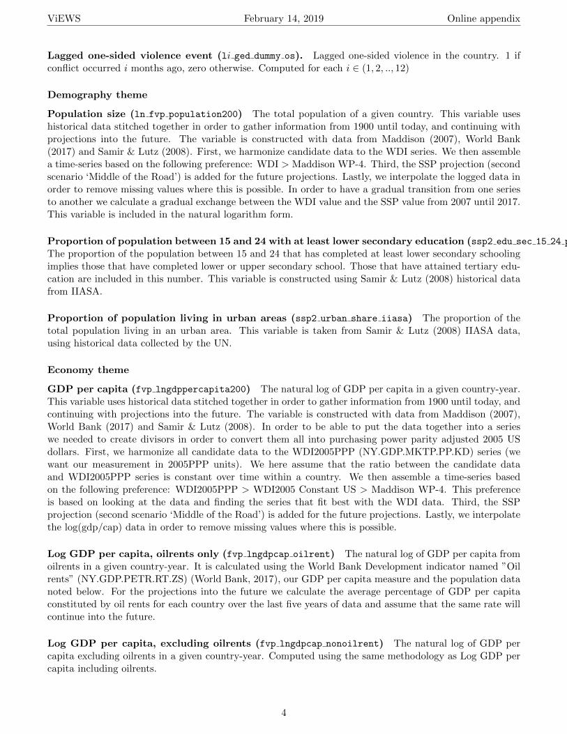
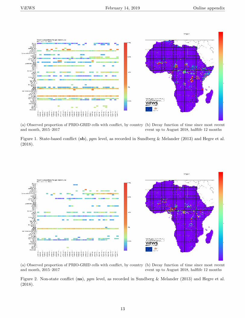
ViEWS generates predictions for the three forms of organized violence coded by the UCDP (Melander,Pettersson & Themner, 2016): State-based conflict (sb), one-sided violence against civilians (os), and non-state conflict (ns).1 Figure 1 summarizes the most recent observations for the sb outcome variables. Figure1a shows the proportion of PRIO-GRID cells with at least one event for each month in the 2015–2017 period.Figure 1b depicts the recent history of violence in each PRIO-GRID cell. Red cells had conflict in August2018, and purple ones have not seen conflict in many years. Figure 2 and 3 show the same for the other twooutcome variables.
Conflict data are primarily obtained from UCDP-GED and take the form of events (Sundberg & Me-lander, 2013). Historical data covering 1989–2017 are extracted from the UCDP GED version 18.1 (Croicu &Sundberg, 2013; Allansson, Melander & Themner, 2017; Pettersson & Eck, 2018).2 Newer data are providedby the new UCDP-Candidate dataset which is updated monthly (see Hegre et al., 2018, for an introduction).This allows using conflict events up to one month before the forecasting window. Here, we use data includingAugust 2018.
We aggregate the UCDP-GED events up to our two levels of analysis.
1See Melander, Pettersson & Themner (2016) and https://www.pcr.uu.se/research/ucdp/definitions/ for detailed def-initions.
2The UCDP-GED raw data are publicly available through the UCDP-GED API.(Croicu & Sundberg, 2013). ViEWSautomatically retrieves these data from the API each month and aggregate to our units of analysis as described in Hegre et al.(2018). Usage of the API is described in http://ucdp.uu.se/apidocs/; the data are available as version 18.1 (1989–2017).
12
ViEWS February 14, 2019 Online appendix
(a) Observed proportion of PRIO-GRID cells with conflict, by countryand month, 2015–2017
(b) Decay function of time since most recentevent up to August 2018, halflife 12 months
Figure 1. State-based conflict (sb), pgm level, as recorded in Sundberg & Melander (2013) and Hegre et al.(2018).
(a) Observed proportion of PRIO-GRID cells with conflict, by countryand month, 2015–2017
(b) Decay function of time since most recentevent up to August 2018, halflife 12 months
Figure 2. Non-state conflict (ns), pgm level, as recorded in Sundberg & Melander (2013) and Hegre et al.(2018).
13

ViEWS February 14, 2019 Online appendix
(a) Observed proportion of PRIO-GRID cells with conflict, by countryand month, 2015–2017
(b) Decay function of time since most recentevent up to August 2018, halflife 12 months
Figure 3. One-sided violence (os), pgm level, as recorded in Sundberg & Melander (2013) and Hegre et al.(2018).
B.3 The persistence of conflict in Africa
Our forecasts for state-based conflict in Africa are very stable over time (Figure 8 in main article and Figure13 below). This to a large degree reflect that conflict patterns have been very persistent over the pastdecade.
Figure 4. Conflict history at three points in time: December 2011 (left), December 2014 (middle), August2018 (right)
Figure 4 shows the recent conflict history at the end of the training period (December 2011) as well asthe end of the calibration period (December 2014). At both points in time, conflicts in Algeria, NorthernNigeria, Sudan, South Sudan, Somalia, and DR Congo were dominating. By 2014, Mali had entered thefray. These conflict hot spots were the same as those dominating the test period (2015–2017), as shownin the right-most map of the situation in August 2018. These conflicts both influenced the training andcalibration of the ensemble and contributed heavily to the conflict history available in December 2014,
14

ViEWS February 14, 2019 Online appendix
and our predictions for these locations were depressingly accurate. Our slow-moving predictors (politicalinstitutions and geography) reinforced this pattern.
B.4 Descriptive statistics
The evaluation metrics we use are dependent on the data they are evaluated for. In particular, they areall in varying ways dependent on class balance. Table 1 shows that the pgm dataset has very strong classimbalance. 0.3% of pgms had state-based conflict events, 0.1% had non-state conflict events, and 0.2% hadone-sided violence.
avg sb 0.003227
avg ns 0.001123
avg os 0.002112
avg decay sb 0.044849
avg decay ns 0.033029
avg decay os 0.039404
stdev decay sb 0.129578
stdev decay ns 0.099688
stdev decay os 0.116185
Table 1. Descriptive statistics of dependent variables 1990-2018. Also includes decay functions of thosedependent variables
C Statistical modeling
C.1 Estimation of constituent models
ViEWS relies on logistic regression and random forest models. The logit model is a generalized linear model(GLM) that performs well compared to many machine-learning techniques (Geron, 2017). Computationalcosts are low, and with large datasets like ours overfitting is not a serious concern. The random forestmodel (Breiman, 2001; Muchlinski et al., 2016) is a machine-learning technique based on a combination ofclassification and regression trees (CART), bootstrap-aggregating (bagging), and random feature selection.In CART, the response variable Y is predicted using a decision tree and some predictor variables X. Thetree consists of a number of ”splits” into different branches. Each split is found by searching all values in Xto find the constant which maximally separates between the categories of Y. The tree continues to be splituntil some threshold is achieved (to avoid overfitting). CART can be combined with bagging to create anensemble of trees, each slightly different. These trees are, however, correlated as some variables are especiallygood at discriminating Y. To avoid this, a random subset of variables (predictors or features) are selectedfor each ‘split’, solving the correlation problem and creating a forest of uncorrelated ‘random’ trees. Becauserandom forest models are computationally intensive, we estimate them using a ‘downsampled’ dataset whichincludes all conflict events and a random sample of non-events (see details in Section E.1 in this appendix).
D Ensemble Bayesian Model Averaging
In ViEWS, we rely on the average prediction from all models to create our ensemble. However, we alsoimplemented an Ensemble Bayesian Model Averaging (EBMA) approach (Montgomery, Hollenbach & Ward,2012; Beger, Dorff & Ward, 2014; Raftery & Lewis, 1992; Raftery et al., 2005). EBMA weighs the constituentmodels before combining them in an ensemble. The weights are based on the performance of the constituentmodels in the calibration period. Overall, we have found that the two approaches yield very similar results(for similar conclusions in a different context, see Graefe et al., 2015).
That the weighted approach of EBMA does not outperform the unweighted (or equally-weighted) averageprediction is potentially because the relative performance of the constituent models varies over time. The
15

ViEWS February 14, 2019 Online appendix
EBMA computes weights so that the performance of the ensemble of constituent models is optimized forthe actual outcomes in the calibration period. However, these weights may not be optimal for other timeperiods (the testing/forecasting period). The conflicts that happened to occur in the calibration period maybe driven by certain factors represented in one or two of our themes (say for example ethnic cleavages orcoup d’etats). If these factors are not equally important in the conflicts that occur in the testing/forecastingperiod, the ensemble suffers from over-fitting to the calibration data. Such clustering of conflict with similarcauses in time (and space) is not unusual, consider for example the numerous conflicts in the immediateaftermath of the breakdown of the Soviet Union or the Arab Spring uprisings. In contrast, the unweightedaverage ensembles are not affected by such temporal fluctuations since the weights are not given by the dataat all.
Another weakness that the EBMA approach shares with the equally-weighted average of predictedprobabilities is that the weights are applied uniformly to all cases. It is possible that some themes are moreimportant in some subsets of the countries or geographical locations in Africa. In that case, models shouldbe weighted differently in different sub-regions. ViEWS will look into various stacking techniques to seewhether these approaches can yield better aggregated forecasts.
Since the EBMA results are very similar to the unweighted average, and EBMA involves considerableadditional complexity, the ViEWS forecasts are currently based on the latter. However, we will continueto combine models using both ensemble methods and expand to other ensemble methods to accumulateevidence on their relative performance for conflict forecasting.
D.1 Combining three types of political violence outcomes
The figures depicting our forecasts (Figures 5 and 7 in the main article, and additional figures in SectionJ), are relatively similar – locations with a high predicted probability of one type of violence also has highrisk of the other two. This partly reflects that the various forms of organized violence occur through relatedprocesses and are constrained by the same factors. In addition, there is considerable spillover between theforms of violence. One-sided violence, for instance, is most frequently perpetrated in the context of a state-based conflict. We believe there is ample scope for improving the system by modeling more carefully howthe three outcomes affect each other and how they are distinct.
Combining these three outcomes in a single system brings several advantages. First, they togetherconstitute a reasonable definition of political violence that subsumes conflicts such as the ongoing war inSyria, the 1994 genocide in Rwanda, and drug-related organized violence in Mexico. The system allowsthem to be modeled separately since they follow different dynamics and involve different types of actors.At the same time, ViEWS allows the various types of violence to serve as early-warning indicators for eachother.
E Downsampling and calibration
E.1 Downsampling
A majority of the models in ViEWS were trained on all available observations. All our random forests,however, were trained on a downsampled dataset. When downsampling, we keep all conflict events andrandomly sample a proportion of the remaining observations. This serves two purposes.
First, it reduces the computational burden. The pgm unit of analysis consists of about 11,000 units forAfrica only. Sampled monthly over the 1990–2014 period for the training dataset, this amounts to a datasetwith about 3.21M rows. Only 13,739 of these – 0.4% – contain observations of UCDP-GED events. Tofacilitate the estimation of the computationally intensive random forest models using this data, we trainedthem on a dataset containing all pgm units with at least one UCDP-GED event and a random sample of10% of the remaining observations.
Second, downsampling is a way of inducing an asymmetric cost-function into our computation. Assumingthat incorrectly predicting peace when there is violence is more costly than predicting violence when there is
16

ViEWS February 14, 2019 Online appendix
actually peace, then we would like our forecasts to hue more closely to predicting the events of violence, evenat the cost of over-estimating some violence in peaceful circumstances. By reducing the proportion of non-events, we also reduce their influence on the fitted models relative to the instances where events occurred.If observations that result in events and non-events are weighted equally, then any unique signal in the rareminority class may be lost. For example, a distinct, but rare, data-generation process might lead to a higherprobability of an event as compared to most observations, which will have a lower probability of an event. Inthis case, downsampling will help our algorithms learn the patterns in cases where violent events occurred,instead of those patterns being treated as random, rare, noise deviating from the more frequent non-events.This should produce higher precision, for example, as compared to non-weighted training where events arehighly infrequent because the model has been trained to work harder to predict events, as compared tonon-downsampled cases (Ricardo Barandela & Rangel, 2003; Chao Chen & Breiman, 2004).
This procedure leads to more predictions of events by artificially shifting the mean upwards. Our cali-bration procedure, described below, transform these predictions so that they in aggregate yield a predictedconflict intensity that is as close to the actual as possible.
E.2 Calibration
Forecasting requires that each model is well calibrated: that the average predicted outcome probabilitiesfor a set of cases is similar to the actual relative frequency for that set. Models that were trained on adownsampled dataset do not have this property, and require calibration. The same applies to the modelsthat are constructed as the product of cm and pgm probabilities. We therefore calibrate the constituentmodel before entering them into the ensemble.
0.0 0.2 0.4 0.6 0.8 1.0
0.0
0.2
0.4
0.6
0.8
1.0
Predicted average, unweighted average ensemble
Obs
erve
d av
erag
e
0.0 0.2 0.4 0.6 0.8 1.0
0.0
0.2
0.4
0.6
0.8
1.0
Predicted average, unweighted average ensemble
Obs
erve
d av
erag
e
0.0 0.2 0.4 0.6 0.8 1.0
0.0
0.2
0.4
0.6
0.8
1.0
Predicted average, unweighted average ensemble
Obs
erve
d av
erag
e
0.0 0.2 0.4 0.6 0.8 1.0
0.0
0.2
0.4
0.6
0.8
1.0
Predicted average, unweighted average ensemble
Obs
erve
d av
erag
e
0.0 0.2 0.4 0.6 0.8 1.0
0.0
0.2
0.4
0.6
0.8
1.0
Predicted average, unweighted average ensemble
Obs
erve
d av
erag
e
0.0 0.2 0.4 0.6 0.8 1.0
0.0
0.2
0.4
0.6
0.8
1.0
Predicted average, unweighted average ensemble
Obs
erve
d av
erag
e
Figure 5. Calibration plots, cm (top) and pgm (bottom) level. Left: sb. Centre: os. Right: ns. Note thatthe x-axis and y-axis is different in the bottom right plot.
We use the calibration partition to calibrate the models. We obtain recentering and rescaling parametersγ0i, γ1i by estimating logistic regression models for each constituent model on the calibration period:
logit(p(Y cv = 1)) = γ0i + γ1iz
civ
where zciv is the log odds of conflict for model i on conflict type v. The rescaling parameters γ0i, γ1i are thenused to shift and strengthen the probabilities in the forecasting period by
pcal(Ycv = 1) =
eγ0i+γ1izciv
e(γ0i+γ1izciv) + 1
17

ViEWS February 14, 2019 Online appendix
0.10
0.15
0.20
0.25
0 6 12 18 24 30 36Month
Act
ual/p
redi
cted
pro
babi
lity
NS
OS
SB
Actual
Predicted
0.002
0.003
0.004
0.005
0 6 12 18 24 30 36Month
Act
ual/p
redi
cted
pro
babi
lity
NS
OS
SB
Actual
Predicted
Figure 6. Calibration over time, cm (left) and pgm (right). The solid lines are smoothed with a loessfunction. Note that the y-axis differs in each plot.
where pcal(Ycv = 1) is our calibrated predicted probability of conflict.
If a model is well calibrated, then an event occurs approximately x percent of the time when the modelsuggests that there is an x percent chance of an event occurring. This can be gauged visually with calibrationplots. In calibration plots, the predicted probabilities are binned on the x-axis and the frequency of actualevents within the observations in each bin is plotted on the y-axis. A perfectly calibrated model follows a 45degree angle. Deviations indicate that the model underpredicts or overpredicts. We show calibration plotsfor our six ensembles in Figure 5. The top panel plots the cm ensembles. Overall, the cm ensembles assignboth too low and too high probabilities. On the left hand side of each plot, we can see that the predictedprobabilities are lower than the actual probability. In the middle of the plots, however, the predictedprobability is too high. The bottom panel plots the pgm ensembles. Here, we can also see that all threeensembles assign both too low and too high probabilities.
We can also evaluate how the calibration of models change over time. In Figure 6, we display the meanactual/predicted probability of conflict on the y-axis, and months in the testing/forecasting period on thex-axis. The colors indicate the conflict type, blue for sb, green for os, and red for ns. Moreover, solid linesare the observed relative frequencies and the dotted lines the predicted probabilities from the unweightedaverage ensembles. Figure 6 shows that the ensembles are relatively well-calibrated. However, it strikingthat the predicted probabilities are relatively constant over time, while the observed relative frequenciesfluctuate. This is to be expected, given that many of the inputs used for forecasting are constant over time.
F Handling missing or incomplete data in ViEWS
F.1 Dependent variables
UCDP-GED includes high-resolution temporal and geographical references. In about 15% of the cases,however, UCDP has been unable to identify the location more precisely than for instance a given second-order administrative region. In such cases, the UCDP assigns the center point of the region as a place-holderlocation and marks the event with a precision score. For prediction purposes, the place-holder solution is notoptimal. Hence, ViEWS has developed a method for multiple imputation of their locations, as documentedin Croicu & Hegre (2018). This method employs the locations of precisely known events within the sameconflict and within close temporal proximity to determine an empirical spatial probability distribution oflatent conflict propensity for each uncertain event. We then sample this empirical probability distributionmultiple times. All the forecasts reported by ViEWS are based on a set of 5 imputed location datasets.Croicu & Hegre (2018) show that this improves the predictive performance of the system considerably.
18
ViEWS February 14, 2019 Online appendix
F.2 Predictors
Some variables in the predictor data used by the ViEWS project contains a certain amount of missing data.This is problematic for several reason. Firstly, making predictions require the data to be complete, i.e.all values for the variables we use to make predictions must be known. Secondly, not using appropriatemethods for handling the missing data in the training models risk creating biased parameter estimatesand/or standard errors (Allison, 2009) which may have an adverse affect on the predictive capabilities ofthe models.
Depending on the mechanisms for how the missingness appear, different missing data methods havedifferent advantages. The most common method for handling missing data is to simply remove all observa-tions which are not complete in listwise deletion (Lall, 2016). Listwise deletion does, however, assume thatthe data are missing completely at random, i.e. that the reason for the missingness is independent both ofthe value of the variable itself and independent of the values of the other variables in the model. In socialsciences this is most often not a reasonable assumption. If it does not hold, the results from the analysiswill be biased (Allison, 2009; ?; ?).
An alternative method for handling missing data which does not require this assumption is imputation.Here, the missing data are replaced (imputed) with some plausible values. Several possible imputationmethods exist. Among the more naive are to use either the mean or the predicted values from a linearregression of the variable on all other variables. Mean and regression imputation do, however, also bias theresults unless some strong assumptions are fulfilled (Buuren, Buuren). The solution to these problems is touse multiple imputation. 3
The ViEWS project uses Multiple Imputation with the Amelia II package in R to replace the missingdata. Amelia II uses bootstrapping and the expectation-maximization (EM) algorithm to impute eachmissing value ( m) times to create m complete datasets. The number of imputations, m, affects a number ofstatistical quantities, including power and efficiency. To achieve reasonable statistical efficiency, as few as 5complete imputed datasets are needed. A higher number of imputations do, however, lead to both higherefficiency and higher power and precision (see for instance Graham, Olchowski & Gilreath, 2007; White,Royston & Wood, 2011). As imputation is computationally intensive in large datasets, and the ViEWSproject due to its focus on prediction is less concerned with statistical power, five imputations are currentlyused. Our dynamic simulation procedure uses all five datasets simultaneously and the results are aggregatedusing the Rubin Rules (Rubin, 1987). In the one-step-ahead forecasts, only one imputed dataset is used atthis time. Using one dataset instead of five will not bias the results, but will reduce the statistical efficiency(Buuren, Buuren).
The ViEWS project will conduct further tests on how different missing data techniques affect predictionand simulation, in order to create a best practice for missing data in predictive studies.
G Detailed evaluation, state-based conflict (sb)
In this section, we present evaluation results for each individual model in the ensemble for sb, biseparationplots, and confusion matrices.
The following metrics are computed (Geron, 2017, pp.86–95):Precision (Pr):
Pr =TP
TP + FP
Recall or Sensitivity (R):
R =TP
TP + FN
Accuracy (A):
3For a more comprehensive test of missing data methods see Randahl (2016).
19
ViEWS February 14, 2019 Online appendix
A =TN + TP
TN + FP + FN + TP
Brier Score:
BS =1
N
N∑i=1
(pi −Ai)2
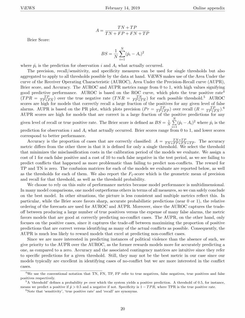
where pi is the prediction for observation i and Ai what actually occurred.The precision, recall/sensitivity, and specificity measures can be used for single thresholds but also
aggregated to apply to all thresholds possible by the data at hand. ViEWS makes use of the Area Under thecurve of the Receiver Operating Characteristic (AUROC), Area Under the Precision-Recall curve (AUPR),Brier score, and Accuracy. The AUROC and AUPR metrics range from 0 to 1, with high values signifyinggood predictive performance. AUROC is based on the ROC curve, which plots the true positive rate4
(TPR = TPTP+FN ) over the true negative rate (TNR = TN
FP+TN ) for each possible threshold.5 AUROCscores are high for models that correctly recall a large fraction of the positives for any given level of falsealarms. AUPR is based on the PR plot, which plots precision (Pr = TP
TP+FP ) over recall (R = TPTP+FN ).6
AUPR scores are high for models that are correct in a large fraction of the positive predictions for any
given level of recall or true positive rate. The Brier score is defined as BS = 1N
N∑i=1
(pi−Ai)2 where pi is the
prediction for observation i and Ai what actually occurred. Brier scores range from 0 to 1, and lower scorescorrespond to better performance.
Accuracy is the proportion of cases that are correctly classified: A = TN+TPTN+FP+FN+TP . The accuracy
metric differs from the other three in that it is defined for only a single threshold. We select the thresholdthat minimizes the misclassification costs in the calibration period of the models we evaluate. We assign acost of 1 for each false positive and a cost of 10 to each false negative in the test period, as we see failing topredict conflicts that happened as more problematic than failing to predict non-conflicts. The reward forTP and TN is zero. The confusion matrices for each of the models we evaluate are reported below, as wellas the thresholds for each of them. We also report the F1-score which is the geometric mean of precisionand recall for that threshold, as well as the threshold probability.
We choose to rely on this suite of performance metrics because model performance is multidimensional.In many model comparisons, one model outperforms others in terms of all measures, so we can safely concludeon the best model. In other situations, the picture is less consistent and multiple metrics reflect this. Inparticular, while the Brier score favors sharp, accurate probabilistic predictions (near 0 or 1), the relativeordering of the forecasts are used for AUROC and AUPR. Moreover, since the AUROC captures the trade-off between producing a large number of true positives versus the expense of many false alarms, the metricfavors models that are good at correctly predicting no-conflict cases. The AUPR, on the other hand, onlyfocuses on the positive cases, since it captures the trade-off between maximizing the proportion of positivepredictions that are correct versus identifying as many of the actual conflicts as possible. Consequently, theAUPR is much less likely to reward models that excel at predicting non-conflict cases.
Since we are more interested in predicting instances of political violence than the absence of such, wegive priority to the AUPR over the AUROC, as the former rewards models more for accurately predicting aone, as compared to a zero. Accuracy and the associated contingency matrices are intuitive since they referto specific predictions for a given threshold. Still, they may not be the best metric in our case since ourmodels typically are excellent in identifying cases of no-conflict but we are more interested in the conflictcases.
4We use the conventional notation that TN, FN, TP, FP refer to true negatives, false negatives, true positives and falsepositives respectively.
5A ‘threshold’ defines a probability p∗ over which the system yields a positive prediction. A threshold of 0.5, for instance,means we predict a positive if p > 0.5 and a negative if not. Specificity is 1 − TPR, where TPR is the true positive rate.
6Note that ‘sensitivity’, ‘true positive rate’ and ‘recall’ are synonyms.
20

ViEWS February 14, 2019 Online appendix
G.1 AUROC, Brier, and AUPR, cm level
Table 2 shows the main evaluation metrics for all the constituent models in the cm-level ensemble, as wellas for the ensemble itself. Models are named according the following convention:
• ‘ds’ and ‘osa’ refers to the way the model handles dynamics (see methodology section in main paper).
• ‘cm’ refers to the level of analysis.
• ‘acled’ or ‘canon’ denotes whether the models are trained on the period for which we have ACLEDdata (1997– ) or the complete dataset (1990– ).
• ‘base’, ‘mean’, ‘demog’, ‘eco’, ‘hist’, ‘inst’, ‘protest’ refers to a theme as listed in Table 2 in the mainpaper. ‘base’ refers to all themes, ‘mean’ to the baseline, ‘demog’ to demography theme, ‘eco’ toeconomy theme, ‘hist’ to conflict history theme, ‘inst’ to institution theme, and ‘protest’ to protesttheme.
• ‘logit fullsample’ and ‘rf downsampled’ refers to the logit and random forest specifications of ‘osa’.
• ‘sb’ refers to conflict type.
• The final line, ‘average basewthematic’ is the ensemble of all the other models.
ROC AUC Brier Score PR AUC
ds cm acled base eval test sb 0.94790 0.06578 0.84879ds cm canon base eval test sb 0.94624 0.06537 0.84145ds cm canon mean eval test sb 0.82375 0.12524 0.67472ds cm canon demog eval test sb 0.75827 0.16109 0.41894
ds cm canon eco eval test sb 0.69813 0.16647 0.42729ds cm canon hist eval test sb 0.94680 0.06918 0.85272ds cm canon inst eval test sb 0.66490 0.16757 0.39481
ds cm canon protest eval test sb 0.70354 0.22020 0.35786osa cm acled base eval test logit fullsample sb 0.95197 0.06883 0.84474osa cm canon base eval test logit fullsample sb 0.95483 0.06569 0.85701osa cm canon mean eval test logit fullsample sb 0.85661 0.13868 0.57983osa cm canon eco eval test logit fullsample sb 0.69165 0.16340 0.46114osa cm canon hist eval test logit fullsample sb 0.94946 0.07051 0.86608osa cm canon inst eval test logit fullsample sb 0.67326 0.16576 0.48685
osa cm canon protest eval test logit fullsample sb 0.68583 0.20764 0.34425osa cm acled base eval test rf downsampled sb 0.95488 0.07184 0.86883osa cm canon base eval test rf downsampled sb 0.95287 0.07362 0.85618
osa cm canon demog eval test logit fullsample sb 0.77214 0.15714 0.42471osa cm canon mean eval test rf downsampled sb 0.86299 0.13158 0.59163osa cm canon demog eval test rf downsampled sb 0.84481 0.13794 0.61618
osa cm canon eco eval test rf downsampled sb 0.76901 0.15406 0.52316osa cm canon hist eval test rf downsampled sb 0.93942 0.08453 0.83937osa cm canon inst eval test rf downsampled sb 0.78731 0.15359 0.62807
osa cm canon protest eval test rf downsampled sb 0.57568 0.17813 0.24507average basewthematic sb 0.95549 0.09318 0.86930
Table 2. SB constituent models and ensembles, cm level, 36 months
Overall, Table 2 shows that there are big differences between the models. As expected, the theme modelsperform poorer than the models with all predictors included. Importantly, while there are a few modelsthat perform similar to the ensemble, the performance of these are likely to fluctuate depending on the timeperiod we use for evaluation. Combining all models in the ensemble therefore adds robustness to the forecast.That said, the ensemble suffers somewhat with respect to the sharpness of predictions in comparison to anumber of other models.
21

ViEWS February 14, 2019 Online appendix
(a) Baseline + history + demography model (horizontally)vs. baseline + history only (vertically)
(b) Ensemble model (horizontally) vs. Baseline + history+ demography model (vertically)
Figure 7. Bi-separation plots, cm level
Bi-separation plots, cm level
To evaluate the difference in performance in more detail, we show bi-separation plots (Colaresi & Mahmood,2017). Figure 7a shows a bi-separation plot for the model combining the baseline, history, and demographythemes on the horizontal axis and the same for the simpler baseline and history model on the vertical, anda scatter plot for each observation in the cm evaluation period. Country-months with observed conflict arerepresented with red color, and no-conflict ones with blue. A number of interesting observations are labeledin the plot. The cluster of blue dots above and to the left of the diagonal are no-conflict observations thathave been ranked much lower in terms of conflict probability by the more extensive model. They refer to anumber of small, relatively well-educated, peaceful countries (e.g., Swaziland and Botswana). The cluster ofblue dots beneath and to the right of the diagonal are another set of peaceful observations that the modelwith demographic characteristics ranks higher than the history-only model. All these refer to Tanzania, avery populous but poor country that has been remarkably peaceful.
The cluster of red dots beneath and to the right of the diagonal are conflict observations that theextensive model yielded a higher predicted probability for, contributing to an improved performance. Thesecases include Tchad in 2015 and Niger in 2015–16, both medium-size countries with low education rates.Finally, the red dots to the left and above the diagonal are conflict observations for which the extensivemodel yielded a lower predicted probability. They include Tunisia, which has high education rates relativeto the African average.
Figure 7b demonstrates the performance of the ensemble model compared to the model including theconflict history and demography themes. The horizontal separation plot shows that the ensemble is muchbetter at sorting out the conflict cases. Adding information from all the other themes in particular improvespredictions of the conflicts in Ethiopia, Tchad, and Tunisia, as well as the absence of violence in Benin,Burkina Faso, and Zambia. Some of the conflict cases that the history + demography model did well on
22

ViEWS February 14, 2019 Online appendix
Figure 8. Model criticism plots
(e.g., in Angola) are less well pointed out by the ensemble, though. Similarly, the ensemble model suggestsa high likelihood of conflict in Zimbabwe, but this conflict did not occur in the evaluation period.
Figure 8 show model criticism plots (also developed by Colaresi & Mahmood, 2017) for the demographyand ensemble models at the cm level. They show that the ensemble is better at identifying positive casesin the test partition – none of the actual conflict months are ranked in the bottom third of predictedprobabilities, a clear improvement relative to the demography model. At the same time, the distribution ofpredicted probabilities are less sharp for the ensemble model.
Figure 9 shows two more bi-separation plots that complement Figure 7. The left-most figure showschanges in ranking of observations when adding the economics theme to the baseline + history only model.The economics predictors increase the predicted probabilities of
Confusion matrices, cm level
Confusion matrices show predicted values of conflict as opposed to observed values (actuals) for the modelsdescribed in Tables 5 and 6 of the article. Since these matrices present binary predictions (positives andnegatives), rather than probabilities, a threshold (cutoff) needs to be chosen. A ‘threshold’ is defined as aprobability p∗ over which the model yields a positive prediction. A threshold of 0.5, for instance, means wepredict a positive if p > 0.5 and a negative if not.
ObservedPredicted Pos Neg SumPos True Posi-
tive (TP)False Posi-tive (FP)
TP + FP
Neg False Neg-ative (FN)
True Neg-ative (TN)
FN + TN
Sum TP + FN FP + TN Total
Table 3. Confusion matrix definitions
23

ViEWS February 14, 2019 Online appendix
●●●●●●● ●●●●
● ●
●●●●
●●
●
●●●●
●●
●
● ●●●●● ● ●●● ●●●
LBR 2015−10BEN 2016−02MWI 2015−09SLE 2015−08LBR 2015−11COM 2015−12SLE 2015−10SLE 2015−11SLE 2015−09LBR 2016−04COG 2017−04COG 2017−12ETH 2015−05ETH 2015−07ETH 2015−11ETH 2015−10ETH 2015−08ETH 2015−12ETH 2016−04ETH 2016−08
ZA
F 2017−
12Z
AF
2017−09
BW
A 2017−
10S
YC
2017−10
BW
A 2017−
12E
TH
2015−01
ET
H 2015−
02E
TH
2015−06
ET
H 2015−
03E
TH
2015−04
BFA
2016−01
TC
D 2015−
06T
CD
2015−10
TC
D 2015−
11N
ER
2015−07
NE
R 2015−
12T
CD
2015−08
NE
R 2015−
11N
ER
2015−10
NE
R 2016−
09
ds_c
m_c
anon
_mea
nhis
t_ev
al_t
est_
sb
ds_cm_canon_meanhisteco_eval_test_sb
●● ●●
●●●
●●
●
●
●●●●●● ●● ●● ●●● ●●●●● ●●●●●● ●● ●●●
MWI 2015−01MWI 2015−03MWI 2015−04MWI 2015−05COM 2015−08MWI 2015−06MWI 2015−09MWI 2015−08MWI 2015−11TZA 2017−06CAF 2015−02ETH 2015−11ETH 2015−08ETH 2015−12ETH 2016−03ETH 2016−04ETH 2016−05ETH 2016−06ETH 2016−07ETH 2016−12
ET
H 2015−
02C
AF
2015−01
CA
F 2015−
11E
TH
2015−01
ET
H 2015−
03C
AF
2015−04
CA
F 2015−
03C
AF
2016−11
CA
F 2015−
05C
AF
2016−10
TU
N 2017−
07E
GY
2016−09
EG
Y 2016−
08E
GY
2016−12
EG
Y 2016−
11E
GY
2017−02
EG
Y 2017−
04E
GY
2017−03
EG
Y 2017−
06E
GY
2017−08
ds_c
m_c
anon
_mea
nhis
t_ev
al_t
est_
sb
ds_cm_canon_meanhistinst_eval_test_sb
Figure 9. Bi-separation plots: Contributions from economics and institutional themes
This cutoff was chosen by minimizing the misclassification costs in the calibration period of the modelswe evaluate. We assign a cost of a false-negative to 10 times the cost of a false-positive, as we consider thatfailing to predict conflict is more problematic than failing to predict non-conflict for both methodologicalreasons (as the classes are highly imbalanced) and practical reasons.
Confusion matrices contain the information described in Table 3 (Geron, 2017, pp. 86–95).Tables 4–10 show confusion matrices for all the models in Table 5 in the main article.
ObservedPredicted Pos Neg SumPos 397 672 1069Neg 57 818 875Sum 454 1490 1944
Note. State-based conflict at cm-level, January2015 to December 2017. Accuracy = 0.625, F1 =0.521, precision = 0.371, recall = 0.874, threshold= 0.132.
Table 4. Baseline
G.2 AUROC, Brier, and AUPR, pgm level
Table 11 shows the main evaluation metrics for all the constituent models in the pgm-level ensemble, as wellas for the ensemble itself. Models are named according the following convention:
• ‘ds’ and ‘osa’ refers to the way the model handles dynamics (see methodology section in main paper).
• ‘pgm’ refers to the level of analysis.
• ‘acled’ or ‘canon’ denotes whether the models are trained on the period for which we have ACLEDdata (1997– ) or the complete dataset (1990– ) for all models except the thematic ones. The thematic
24

ViEWS February 14, 2019 Online appendix
ObservedPredicted Pos Neg SumPos 411 245 656Neg 43 1245 1288Sum 454 1490 1944
Note. State-based conflict at cm-level, January2015 to December 2017. Accuracy = 0.852, F1 =0.741, precision = 0.627, recall = 0.905, threshold= 0.055.
Table 5. Baseline + conflict history theme
ObservedPredicted Pos Neg SumPos 399 191 590Neg 55 1299 1354Sum 454 1490 1944
Note. State-based conflict at cm-level, January2015 to December 2017. Accuracy = 0.873, F1 =0.764, precision = 0.676, recall = 0.879, threshold= 0.083.
Table 6. Baseline + history + economics themes
models have acled in the name even though they are estimated on the complete dataset. This strictlya labelling issues due to a technicality in the database processing.
• ‘nocm’, ‘wcm’, ‘cl’, ‘mean’, ‘soc’, ‘nat’, ‘histonly’, ‘cm’, ‘protest’ refers to a theme as listed in Table 3in the main paper. ‘nocm’ refers to all themes without cm level predictors, ‘wcm’ and ‘cl’ refer to allthemes including cm level predictors either in the pgm model specification or multiplied probabilitiesas explained in the methodology section of the main article, ‘mean’ to the baseline, ‘soc’ to socialgeography theme, ‘nat’ to natural geography theme, ‘histonly’ to conflict history theme, ‘cm’ to cmtheme, and ‘protest’ to protest theme.
• ‘logit fullsample’ and ‘rf downsampled’ refers to the logit and random forest specifications of ‘osa’.
• ‘sb’ refers to conflict type.
• The final line, ‘average allwthematic’ is the ensemble of all the other models.
Similar to the cm level evaluation, Table 11 shows that there are big differences between the models atthe pgm level. As expected, the theme models perform poorer than the models with all predictors included.Interestingly, the sharpness of predictions is very similar across models here, as compared to the cm levelevaluation.
Confusion matrices, pgm level
Tables 12–16 show the confusion matrices for the models we evaluate at the pgm level (Table 6 in mainarticle).
25

ViEWS February 14, 2019 Online appendix
ObservedPredicted Pos Neg SumPos 426 354 780Neg 28 1136 1164Sum 454 1490 1944
Note. State-based conflict at cm-level, January2015 to December 2017. Accuracy = 0.803, F1 =0.69, precision = 0.546, recall = 0.938, threshold =0.09.
Table 7. Baseline + history + demography themes
ObservedPredicted Pos Neg SumPos 374 58 432Neg 80 1432 1512Sum 454 1490 1944
Note. State-based conflict at cm-level, January2015 to December 2017. Accuracy = 0.929, F1 =0.844, precision = 0.866, recall = 0.824, threshold= 0.724.
Table 8. Baseline + history + institutions themes
ObservedPredicted Pos Neg SumPos 436 512 948Neg 18 978 996Sum 454 1490 1944
Note. State-based conflict at cm-level, January2015 to December 2017. Accuracy = 0.727, F1 =0.622, precision = 0.46, recall = 0.96, threshold =0.089.
Table 9. All themes
ObservedPredicted Pos Neg SumPos 437 282 719Neg 17 1208 1225Sum 454 1490 1944
Note. State-based conflict at cm-level, January2015 to December 2017. Accuracy = 0.846, F1 =0.745, precision = 0.608, recall = 0.963, threshold= 0.126.
Table 10. Ensemble
26

ViEWS February 14, 2019 Online appendix
ROC AUC Brier Score PR AUC
ds pgm canon nocm eval test sb 0.91639 0.00670 0.23576ds pgm canon wcm eval test sb 0.90922 0.00646 0.25480ds pgm acled nocm eval test sb 0.92204 0.00638 0.24544
cl ds pgm canon nocm eval test sb 0.92663 0.00640 0.21426ds pgm acled soc eval test sb 0.75885 0.00657 0.01878ds pgm acled nat eval test sb 0.74278 0.00657 0.01383
ds pgm acled mean eval test sb 0.63240 0.00657 0.04874ds pgm acled histonly eval test sb 0.89488 0.00685 0.21931ds pgm acled protest eval test sb 0.66140 0.00657 0.01248
ds pgm acled cm eval test sb 0.59921 0.00657 0.00585osa pgm acled nocm eval test logit fullsample sb 0.93033 0.00612 0.25824osa pgm canon nocm eval test logit fullsample sb 0.92955 0.00610 0.26148osa pgm canon wcm eval test logit fullsample sb 0.92510 0.00617 0.24607
cl osa pgm canon nocm eval test logit fullsample sb 0.93727 0.00612 0.25479osa pgm acled soc eval test logit fullsample sb 0.76909 0.00657 0.01721osa pgm acled nat eval test logit fullsample sb 0.75525 0.00657 0.01318
osa pgm acled mean eval test logit fullsample sb 0.86800 0.00664 0.07008osa pgm acled histonly eval test logit fullsample sb 0.92198 0.00616 0.24726osa pgm acled protest eval test logit fullsample sb 0.70775 0.00657 0.01588
osa pgm acled cm eval test logit fullsample sb 0.55844 0.00657 0.00501osa pgm acled nocm eval test rf downsampled sb 0.94519 0.00623 0.23495osa pgm canon nocm eval test rf downsampled sb 0.94481 0.00623 0.22896osa pgm canon wcm eval test rf downsampled sb 0.94781 0.00618 0.24163
cl osa pgm canon nocm eval test rf downsampled sb 0.94615 0.00624 0.22618osa pgm acled soc eval test rf downsampled sb 0.91338 0.00646 0.17248osa pgm acled nat eval test rf downsampled sb 0.90216 0.00654 0.15135
osa pgm acled mean eval test rf downsampled sb 0.88153 0.00657 0.07407osa pgm acled histonly eval test rf downsampled sb 0.93301 0.00626 0.23359osa pgm acled protest eval test rf downsampled sb 0.67398 0.00657 0.01360
osa pgm acled cm eval test rf downsampled sb 0.78972 0.00657 0.02489average allwthematic sb 0.94839 0.00623 0.27689
Table 11. SB constituent models and ensembles, pgm level, 36 months
ObservedPredicted Pos Neg SumPos 234 1046 1280Neg 1426 381558 382984Sum 1660 382604 384264
Note. State-based conflict at pgm-level, January2015 to December 2017. Accuracy = 0.994, F1 =0.159, precision = 0.183, recall = 0.141, threshold= 0.017.
Table 12. Baseline
ObservedPredicted Pos Neg SumPos 797 3623 4420Neg 863 378981 379844Sum 1660 382604 384264
Note. State-based conflict at pgm-level, January2015 to December 2017. Accuracy = 0.988, F1 =0.262, precision = 0.18, recall = 0.48, threshold =0.066.
Table 13. Baseline + history themes
27

ViEWS February 14, 2019 Online appendix
ObservedPredicted Pos Neg SumPos 605 2085 2690Neg 1055 380519 381574Sum 1660 382604 384264
Note. State-based conflict at pgm-level, January2015 to December 2017. Accuracy = 0.992, F1 =0.278, precision = 0.225, recall = 0.364, threshold= 0.141.
Table 14. Baseline + history + social and natural geography themes
ObservedPredicted Pos Neg SumPos 639 2726 3365Neg 1021 379878 380899Sum 1660 382604 384264
Note. State-based conflict at pgm-level, January2015 to December 2017. Accuracy = 0.99, F1 =0.254, precision = 0.19, recall = 0.385, threshold =0.11.
Table 15. All themes
ObservedPredicted Pos Neg SumPos 735 2706 3441Neg 925 379898 380823Sum 1660 382604 384264
Note. State-based conflict at pgm-level, January2015 to December 2017. Accuracy = 0.991, F1 =0.289, precision = 0.214, recall = 0.443, threshold= 0.064.
Table 16. Ensemble
28
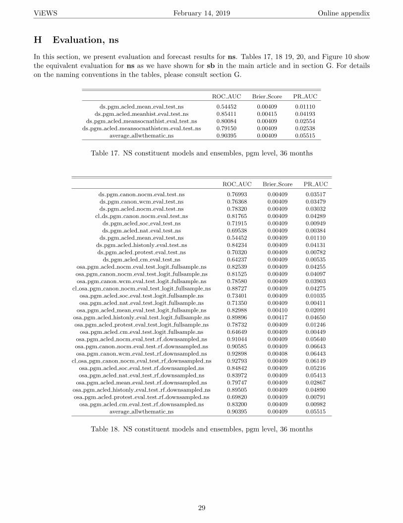
ViEWS February 14, 2019 Online appendix
H Evaluation, ns
In this section, we present evaluation and forecast results for ns. Tables 17, 18 19, 20, and Figure 10 showthe equivalent evaluation for ns as we have shown for sb in the main article and in section G. For detailson the naming conventions in the tables, please consult section G.
ROC AUC Brier Score PR AUC
ds pgm acled mean eval test ns 0.54452 0.00409 0.01110ds pgm acled meanhist eval test ns 0.85411 0.00415 0.04193
ds pgm acled meansocnathist eval test ns 0.80084 0.00409 0.02554ds pgm acled meansocnathistcm eval test ns 0.79150 0.00409 0.02538
average allwthematic ns 0.90395 0.00409 0.05515
Table 17. NS constituent models and ensembles, pgm level, 36 months
ROC AUC Brier Score PR AUC
ds pgm canon nocm eval test ns 0.76993 0.00409 0.03517ds pgm canon wcm eval test ns 0.76368 0.00409 0.03479ds pgm acled nocm eval test ns 0.78320 0.00409 0.03032
cl ds pgm canon nocm eval test ns 0.81765 0.00409 0.04289ds pgm acled soc eval test ns 0.71915 0.00409 0.00949ds pgm acled nat eval test ns 0.69538 0.00409 0.00384
ds pgm acled mean eval test ns 0.54452 0.00409 0.01110ds pgm acled histonly eval test ns 0.84234 0.00409 0.04131ds pgm acled protest eval test ns 0.70320 0.00409 0.00782
ds pgm acled cm eval test ns 0.64237 0.00409 0.00535osa pgm acled nocm eval test logit fullsample ns 0.82539 0.00409 0.04255osa pgm canon nocm eval test logit fullsample ns 0.81525 0.00409 0.04097osa pgm canon wcm eval test logit fullsample ns 0.78580 0.00409 0.03903
cl osa pgm canon nocm eval test logit fullsample ns 0.88727 0.00409 0.04275osa pgm acled soc eval test logit fullsample ns 0.73401 0.00409 0.01035osa pgm acled nat eval test logit fullsample ns 0.71350 0.00409 0.00411
osa pgm acled mean eval test logit fullsample ns 0.82988 0.00410 0.02091osa pgm acled histonly eval test logit fullsample ns 0.89896 0.00417 0.04650osa pgm acled protest eval test logit fullsample ns 0.78732 0.00409 0.01246
osa pgm acled cm eval test logit fullsample ns 0.64649 0.00409 0.00449osa pgm acled nocm eval test rf downsampled ns 0.91044 0.00409 0.05640osa pgm canon nocm eval test rf downsampled ns 0.90585 0.00409 0.06643osa pgm canon wcm eval test rf downsampled ns 0.92898 0.00408 0.06443
cl osa pgm canon nocm eval test rf downsampled ns 0.92793 0.00409 0.06149osa pgm acled soc eval test rf downsampled ns 0.84842 0.00409 0.05216osa pgm acled nat eval test rf downsampled ns 0.83972 0.00409 0.05413
osa pgm acled mean eval test rf downsampled ns 0.79747 0.00409 0.02867osa pgm acled histonly eval test rf downsampled ns 0.89505 0.00409 0.04890osa pgm acled protest eval test rf downsampled ns 0.69820 0.00409 0.00791
osa pgm acled cm eval test rf downsampled ns 0.83200 0.00409 0.00982average allwthematic ns 0.90395 0.00409 0.05515
Table 18. NS constituent models and ensembles, pgm level, 36 months
29

ViEWS February 14, 2019 Online appendix
ROC AUC Brier Score PR AUC
ds cm canon mean eval test ns 0.79469 0.08691 0.54263ds cm canon meanhist eval test ns 0.96404 0.05837 0.77836
ds cm canon meanhisteco eval test ns 0.82576 0.07331 0.59396ds cm canon meanhistdemog eval test ns 0.89656 0.07837 0.68546
ds cm canon meanhistinst eval test ns 0.81799 0.06981 0.62667ds cm acled mndmgecohstnst eval test ns 0.87963 0.07915 0.57454
average basewthematic ns 0.94837 0.07318 0.72198
Table 19. NS constituent models and ensembles, cm level, 36 months
ROC AUC Brier Score PR AUC
ds cm acled base eval test ns 0.94707 0.06547 0.72842ds cm canon base eval test ns 0.95328 0.06335 0.74951ds cm canon mean eval test ns 0.79469 0.08691 0.54263ds cm canon demog eval test ns 0.70675 0.09694 0.40876
ds cm canon eco eval test ns 0.70228 0.11048 0.23194ds cm canon hist eval test ns 0.96519 0.06132 0.78931ds cm canon inst eval test ns 0.39043 0.11780 0.12344
ds cm canon protest eval test ns 0.73217 0.10393 0.21929osa cm acled base eval test logit fullsample ns 0.93679 0.06975 0.64575osa cm canon base eval test logit fullsample ns 0.94566 0.06629 0.68087osa cm canon mean eval test logit fullsample ns 0.87932 0.08863 0.43815osa cm canon eco eval test logit fullsample ns 0.75232 0.10738 0.32756osa cm canon hist eval test logit fullsample ns 0.95552 0.05608 0.68121osa cm canon inst eval test logit fullsample ns 0.60653 0.10899 0.19035
osa cm canon protest eval test logit fullsample ns 0.76011 0.10359 0.25260osa cm acled base eval test rf downsampled ns 0.94828 0.06033 0.68120osa cm canon base eval test rf downsampled ns 0.94254 0.06533 0.63387
osa cm canon demog eval test logit fullsample ns 0.71601 0.09895 0.40929osa cm canon mean eval test rf downsampled ns 0.88006 0.09173 0.46776osa cm canon demog eval test rf downsampled ns 0.87773 0.08971 0.50941
osa cm canon eco eval test rf downsampled ns 0.63579 0.10680 0.23110osa cm canon hist eval test rf downsampled ns 0.93470 0.06095 0.66823osa cm canon inst eval test rf downsampled ns 0.75085 0.09821 0.40758
osa cm canon protest eval test rf downsampled ns 0.74649 0.10442 0.22113average basewthematic sb 0.91552 0.08258 0.52357
Table 20. NS constituent models and ensembles, cm level, 36 months
30
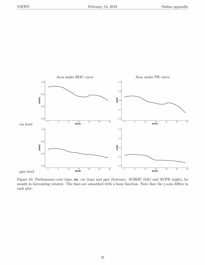
ViEWS February 14, 2019 Online appendix
Area under ROC curve Area under PR curve
cm level
0.85
0.90
0.95
1.00
0 6 12 18 24 30 36Month
AU
RO
C
0.6
0.7
0.8
0.9
1.0
0 6 12 18 24 30 36Month
AU
PR
pgm level
0.85
0.90
0.95
1.00
0 6 12 18 24 30 36Month
AU
RO
C
0.0
0.1
0.2
0.3
0.4
0 6 12 18 24 30 36Month
AU
PR
Figure 10. Performance over time, ns, cm (top) and pgm (bottom). AUROC (left) and AUPR (right), bymonth in forecasting window. The lines are smoothed with a loess function. Note that the y-axis differs ineach plot.
31

ViEWS February 14, 2019 Online appendix
I Evaluation, os
In this section, we present evaluation and forecast results for os. Tables 21, 22, 23, 24, and Figure 11 showthe equivalent evaluation for os as we have shown for sb in the main article and in section G. For detailson the naming conventions in the tables, please consult this section.
ROC AUC Brier Score PR AUC
ds pgm acled mean eval test os 0.61381 0.00527 0.04988ds pgm acled meanhist eval test os 0.87787 0.00572 0.15748
ds pgm acled meansocnathist eval test os 0.90279 0.00578 0.14525ds pgm acled meansocnathistcm eval test os 0.90997 0.00542 0.15596
average allwthematic os 0.94798 0.00513 0.20727
Table 21. OS constituent models and ensembles, pgm level, 36 months
ROC AUC Brier Score PR AUC
ds pgm canon nocm eval test os 0.88843 0.00554 0.16020ds pgm canon wcm eval test os 0.90436 0.00552 0.15702ds pgm acled nocm eval test os 0.90142 0.00523 0.16867
cl ds pgm canon nocm eval test os 0.90993 0.00527 0.15201ds pgm acled soc eval test os 0.80585 0.00527 0.01504ds pgm acled nat eval test os 0.77734 0.00527 0.01245
ds pgm acled mean eval test os 0.61381 0.00527 0.04988ds pgm acled histonly eval test os 0.87696 0.00547 0.15438ds pgm acled protest eval test os 0.69981 0.00527 0.01166
ds pgm acled cm eval test os 0.72482 0.00527 0.00606osa pgm acled nocm eval test logit fullsample os 0.92599 0.00509 0.17936osa pgm canon nocm eval test logit fullsample os 0.91357 0.00506 0.18852osa pgm canon wcm eval test logit fullsample os 0.92163 0.00506 0.18571
cl osa pgm canon nocm eval test logit fullsample os 0.92489 0.00507 0.17957osa pgm acled soc eval test logit fullsample os 0.81256 0.00527 0.01463osa pgm acled nat eval test logit fullsample os 0.79434 0.00527 0.01259
osa pgm acled mean eval test logit fullsample os 0.83820 0.00525 0.07241osa pgm acled histonly eval test logit fullsample os 0.91773 0.00520 0.17616osa pgm acled protest eval test logit fullsample os 0.68571 0.00527 0.01409
osa pgm acled cm eval test logit fullsample os 0.73657 0.00527 0.00582osa pgm acled nocm eval test rf downsampled os 0.94177 0.00515 0.18749osa pgm canon nocm eval test rf downsampled os 0.93976 0.00517 0.18518osa pgm canon wcm eval test rf downsampled os 0.94159 0.00511 0.17709
cl osa pgm canon nocm eval test rf downsampled os 0.94163 0.00515 0.17067osa pgm acled soc eval test rf downsampled os 0.90169 0.00527 0.13447osa pgm acled nat eval test rf downsampled os 0.87855 0.00527 0.10655
osa pgm acled mean eval test rf downsampled os 0.84481 0.00527 0.08377osa pgm acled histonly eval test rf downsampled os 0.91981 0.00527 0.16809osa pgm acled protest eval test rf downsampled os 0.66915 0.00527 0.00990
osa pgm acled cm eval test rf downsampled os 0.80703 0.00527 0.01583average allwthematic os 0.94798 0.00513 0.20727
Table 22. OS constituent models and ensembles, pgm level, 36 months
32

ViEWS February 14, 2019 Online appendix
ROC AUC Brier Score PR AUC
ds cm canon mean eval test os 0.75262 0.13773 0.55828ds cm canon meanhist eval test os 0.91740 0.07919 0.77562
ds cm canon meanhisteco eval test os 0.87062 0.08672 0.72667ds cm canon meanhistdemog eval test os 0.87695 0.08902 0.64605
ds cm canon meanhistinst eval test os 0.83577 0.09006 0.64326ds cm acled mndmgecohstnst eval test os 0.90402 0.08603 0.70878
average basewthematic os 0.93448 0.10264 0.80914
Table 23. OS constituent models and ensembles, cm level, 36 months
ROC AUC Brier Score PR AUC
ds cm acled base eval test os 0.92992 0.07827 0.80586ds cm canon base eval test os 0.92682 0.08238 0.79209ds cm canon mean eval test os 0.75262 0.13773 0.55828ds cm canon demog eval test os 0.74827 0.14640 0.37405
ds cm canon eco eval test os 0.76830 0.14212 0.42117ds cm canon hist eval test os 0.92318 0.07741 0.75591ds cm canon inst eval test os 0.63214 0.15888 0.30793
ds cm canon protest eval test os 0.70661 0.14508 0.30143osa cm acled base eval test logit fullsample os 0.92139 0.07868 0.75031osa cm canon base eval test logit fullsample os 0.92389 0.07903 0.79501osa cm canon mean eval test logit fullsample os 0.81506 0.12884 0.53952osa cm canon eco eval test logit fullsample os 0.73579 0.14509 0.44790osa cm canon hist eval test logit fullsample os 0.91101 0.07905 0.79067osa cm canon inst eval test logit fullsample os 0.61018 0.15861 0.34459
osa cm canon protest eval test logit fullsample os 0.68593 0.14667 0.29725osa cm acled base eval test rf downsampled os 0.91851 0.08234 0.77968osa cm canon base eval test rf downsampled os 0.91659 0.08405 0.77511
osa cm canon demog eval test logit fullsample os 0.76597 0.14606 0.38501osa cm canon mean eval test rf downsampled os 0.83186 0.13876 0.57761osa cm canon demog eval test rf downsampled os 0.79102 0.13662 0.50908
osa cm canon eco eval test rf downsampled os 0.76807 0.14320 0.43615osa cm canon hist eval test rf downsampled os 0.90722 0.08258 0.76523osa cm canon inst eval test rf downsampled os 0.74552 0.14753 0.50227
osa cm canon protest eval test rf downsampled os 0.61866 0.15853 0.22503average basewthematic sb 0.91384 0.10069 0.69488
Table 24. OS constituent models and ensembles, cm level, 36 months
33

ViEWS February 14, 2019 Online appendix
Area under ROC curve Area under PR curve
cm level
0.85
0.90
0.95
1.00
0 6 12 18 24 30 36Month
AU
RO
C
0.6
0.7
0.8
0.9
1.0
0 6 12 18 24 30 36Month
AU
PR
pgm level
0.85
0.90
0.95
1.00
0 6 12 18 24 30 36Month
AU
RO
C
0.0
0.1
0.2
0.3
0.4
0 6 12 18 24 30 36Month
AU
PR
Figure 11. Performance over time, os, cm (top) and pgm (bottom). AUROC (left) and AUPR (right), bymonth in forecasting window. The lines are smoothed with a loess function. Note that the y-axis differs ineach plot.
34

ViEWS February 14, 2019 Online appendix
J Additional forecasting results
Figure 12 takes a closer look at Western Central Africa over time. There is a sizeable orange cluster, withprobabilities around 30–50% in each pgm in the Eastern DRC and Burundi for June 2018. This cluster isslowly expanding over the forecasting period, and spills into Rwanda. As clear from Figure 8 in the mainarticle, forecasted conflict patterns are very stable.
sb,pgm, October 2018 sb,pgm, October 2019 sb,pgm, October 2021
Figure 12. Forecasts October 2018 – August 2021, state-based conflict, DRC, CAR, Rwanda, Burundi
2018
-09
2018
-10
2018
-11
2018
-12
2019
-01
2019
-02
2019
-03
2019
-04
2019
-05
2019
-06
2019
-07
2019
-08
2019
-09
2019
-10
2019
-11
2019
-12
2020
-01
2020
-02
2020
-03
2020
-04
2020
-05
2020
-06
2020
-07
2020
-08
2020
-09
2020
-10
2020
-11
2020
-12
2021
-01
2021
-02
2021
-03
2021
-04
2021
-05
2021
-06
2021
-07
2021
-08
2021
-09
2021
-10
AlgeriaAngolaBenin
BotswanaBurkina Faso
BurundiCameroon
Cape VerdeCentral African Republic
ChadComoros
CongoCongo, DRC
Cote d'IvoireDjibouti
EgyptEquatorial Guinea
EritreaEthiopia
GabonGhanaGuinea
Guinea-BissauKenya
LesothoLiberia
LibyaMadagascar
MalawiMali
MauritaniaMauritiusMorocco
MozambiqueNamibia
NigerNigeria
RwandaSao Tome and Principe
SenegalSeychelles
Sierra LeoneSomalia
South AfricaSouth Sudan
SudanSwazilandTanzania
The GambiaTogo
TunisiaUgandaZambia
Zimbabwe
Country proportions for average_all_sb Ensemble run: r.2018.10.01
0.5%
5%
40%
90%
99%
Figure 13. Predicted proportion of PRIO-GRID cells with conflict, by country and month, September2018–October 2021, sb
35

ViEWS February 14, 2019 Online appendix
Country name 2018-10 2019-10 2020-10 2021-10Algeria 0.0016 0.0019 0.0021 0.0021Angola 0.0018 0.0022 0.0025 0.0025Benin 0.0009 0.0012 0.0013 0.0015Botswana 0.0003 0.0003 0.0004 0.0004Burkina Faso 0.0080 0.0058 0.0050 0.0048Burundi 0.2507 0.2680 0.2757 0.2691Cameroon 0.0257 0.0218 0.0203 0.0193Cape Verde 0.0005 0.0006 0.0007 0.0008Central African Republic 0.0058 0.0054 0.0055 0.0059Chad 0.0015 0.0015 0.0017 0.0018Comoros 0.0010 0.0013 0.0013 0.0015Congo 0.0014 0.0017 0.0017 0.0018Congo, DRC 0.0141 0.0145 0.0147 0.0145Cote d’Ivoire 0.0012 0.0017 0.0021 0.0026Djibouti 0.0014 0.0018 0.0022 0.0025Egypt 0.0017 0.0017 0.0017 0.0018Equatorial Guinea 0.0018 0.0024 0.0025 0.0025Eritrea 0.0011 0.0015 0.0016 0.0017Ethiopia 0.0098 0.0122 0.0127 0.0133Gabon 0.0004 0.0005 0.0006 0.0006Ghana 0.0007 0.0010 0.0011 0.0012Guinea 0.0018 0.0022 0.0023 0.0023Guinea-Bissau 0.0015 0.0020 0.0018 0.0019Kenya 0.0095 0.0097 0.0091 0.0089Lesotho 0.0006 0.0008 0.0009 0.0010Liberia 0.0011 0.0015 0.0016 0.0020Libya 0.0024 0.0023 0.0024 0.0024Madagascar 0.0010 0.0014 0.0016 0.0017Malawi 0.0013 0.0019 0.0022 0.0024Mali 0.0100 0.0074 0.0068 0.0062Mauritania 0.0004 0.0005 0.0006 0.0006Mauritius 0.0009 0.0012 0.0013 0.0016Morocco 0.0008 0.0012 0.0014 0.0016Mozambique 0.0055 0.0050 0.0048 0.0045Namibia 0.0002 0.0003 0.0003 0.0003Niger 0.0029 0.0028 0.0027 0.0027Nigeria 0.0241 0.0264 0.0266 0.0270Rwanda 0.0623 0.0716 0.0890 0.1115Sao Tome and Principe 0.0009 0.0011 0.0012 0.0013Senegal 0.0030 0.0033 0.0033 0.0035Seychelles 0.0007 0.0008 0.0010 0.0010Sierra Leone 0.0012 0.0018 0.0021 0.0025Somalia 0.0226 0.0225 0.0217 0.0216South Africa 0.0008 0.0009 0.0010 0.0011South Sudan 0.0057 0.0060 0.0059 0.0056Sudan 0.0041 0.0045 0.0047 0.0047Swaziland 0.0009 0.0011 0.0012 0.0014Tanzania 0.0011 0.0015 0.0017 0.0020The Gambia 0.0046 0.0052 0.0049 0.0059Togo 0.0027 0.0030 0.0027 0.0028Tunisia 0.0037 0.0040 0.0042 0.0049Uganda 0.0144 0.0147 0.0160 0.0169Zambia 0.0005 0.0006 0.0006 0.0007Zimbabwe 0.0027 0.0027 0.0029 0.0030
Table 25. Country proportions (sb)
36

ViEWS February 14, 2019 Online appendix
Figure 14 and Table 26 shows the forecasts in the same form for ns conflict, and Figure 15 and Table27 for one-sided violence.
Figure 14. Predicted proportion of PRIO-GRID cells with conflict, by country and month, September2018–October 2021, ns
Figure 13 shows the forecasted share of PRIO-GRID cells in conflict by country and by month for allthree outcomes (as in Figure 8 in the main article). Table 25 shows the same information in table form forselected months. The forecasted proportion of grid cells with at least one event of state-based conflict in forinstance Burundi is .25 in October 2018 and remains stable until October 2021. The forecasted proportionin Ethiopia starts at 0.010 in October 2018 and increases up to 0.013 at the end of the forecasting window.
37

ViEWS February 14, 2019 Online appendix
Country name 2018-10 2019-10 2020-10 2021-10Algeria 0.0006 0.0008 0.0010 0.0011Angola 0.0007 0.0009 0.0011 0.0011Benin 0.0017 0.0020 0.0022 0.0022Botswana 0.0007 0.0008 0.0008 0.0008Burkina Faso 0.0017 0.0023 0.0024 0.0026Burundi 0.0112 0.0170 0.0209 0.0246Cameroon 0.0024 0.0032 0.0037 0.0040Cape Verde 0.0012 0.0012 0.0014 0.0014Central African Republic 0.0059 0.0060 0.0061 0.0052Chad 0.0012 0.0014 0.0015 0.0015Comoros 0.0017 0.0019 0.0018 0.0020Congo 0.0006 0.0007 0.0007 0.0007Congo, DRC 0.0049 0.0055 0.0059 0.0060Cote d’Ivoire 0.0017 0.0022 0.0026 0.0027Djibouti 0.0012 0.0012 0.0011 0.0012Egypt 0.0008 0.0011 0.0011 0.0013Equatorial Guinea 0.0007 0.0009 0.0010 0.0010Eritrea 0.0010 0.0012 0.0012 0.0013Ethiopia 0.0063 0.0069 0.0071 0.0072Gabon 0.0004 0.0004 0.0005 0.0005Ghana 0.0015 0.0019 0.0022 0.0023Guinea 0.0013 0.0017 0.0018 0.0019Guinea-Bissau 0.0012 0.0014 0.0013 0.0014Kenya 0.0082 0.0085 0.0085 0.0085Lesotho 0.0013 0.0018 0.0017 0.0019Liberia 0.0011 0.0013 0.0016 0.0017Libya 0.0025 0.0024 0.0023 0.0022Madagascar 0.0012 0.0014 0.0015 0.0015Malawi 0.0013 0.0016 0.0018 0.0019Mali 0.0047 0.0038 0.0037 0.0038Mauritania 0.0005 0.0005 0.0006 0.0007Mauritius 0.0018 0.0021 0.0023 0.0025Morocco 0.0010 0.0013 0.0014 0.0015Mozambique 0.0010 0.0012 0.0014 0.0015Namibia 0.0006 0.0006 0.0007 0.0007Niger 0.0011 0.0012 0.0013 0.0013Nigeria 0.0253 0.0257 0.0258 0.0247Rwanda 0.0044 0.0075 0.0108 0.0154Sao Tome and Principe 0.0010 0.0010 0.0011 0.0013Senegal 0.0016 0.0020 0.0024 0.0025Seychelles 0.0016 0.0018 0.0018 0.0018Sierra Leone 0.0013 0.0016 0.0018 0.0019Somalia 0.0059 0.0059 0.0058 0.0063South Africa 0.0015 0.0017 0.0019 0.0020South Sudan 0.0048 0.0044 0.0043 0.0043Sudan 0.0040 0.0044 0.0045 0.0045Swaziland 0.0009 0.0012 0.0010 0.0012Tanzania 0.0012 0.0015 0.0017 0.0018The Gambia 0.0021 0.0027 0.0027 0.0028Togo 0.0016 0.0019 0.0020 0.0022Tunisia 0.0016 0.0021 0.0023 0.0026Uganda 0.0030 0.0046 0.0055 0.0063Zambia 0.0007 0.0009 0.0010 0.0010Zimbabwe 0.0013 0.0020 0.0020 0.0023
Table 26. Country proportions (ns)
Figure 15. Predicted proportion of PRIO-GRID cells with conflict, by country and month, September2018–October 2021, os
38
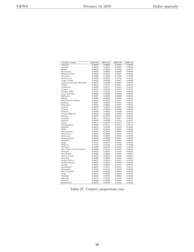
ViEWS February 14, 2019 Online appendix
Country name 2018-10 2019-10 2020-10 2021-10Algeria 0.0006 0.0006 0.0007 0.0007Angola 0.0016 0.0018 0.0019 0.0019Benin 0.0016 0.0020 0.0023 0.0027Botswana 0.0004 0.0004 0.0005 0.0005Burkina Faso 0.0059 0.0052 0.0047 0.0048Burundi 0.1906 0.1844 0.1769 0.1659Cameroon 0.0192 0.0168 0.0152 0.0148Cape Verde 0.0005 0.0006 0.0007 0.0008Central African Republic 0.0092 0.0096 0.0087 0.0079Chad 0.0014 0.0016 0.0017 0.0019Comoros 0.0008 0.0011 0.0012 0.0014Congo 0.0012 0.0013 0.0013 0.0013Congo, DRC 0.0121 0.0125 0.0130 0.0126Cote d’Ivoire 0.0020 0.0029 0.0034 0.0041Djibouti 0.0007 0.0009 0.0009 0.0012Egypt 0.0008 0.0008 0.0009 0.0010Equatorial Guinea 0.0014 0.0015 0.0017 0.0017Eritrea 0.0007 0.0009 0.0010 0.0010Ethiopia 0.0056 0.0062 0.0057 0.0057Gabon 0.0004 0.0005 0.0005 0.0005Ghana 0.0015 0.0020 0.0022 0.0023Guinea 0.0032 0.0043 0.0046 0.0047Guinea-Bissau 0.0018 0.0023 0.0025 0.0027Kenya 0.0073 0.0077 0.0071 0.0065Lesotho 0.0011 0.0016 0.0017 0.0018Liberia 0.0020 0.0028 0.0031 0.0037Libya 0.0011 0.0010 0.0010 0.0010Madagascar 0.0009 0.0011 0.0013 0.0014Malawi 0.0014 0.0020 0.0023 0.0025Mali 0.0055 0.0043 0.0038 0.0036Mauritania 0.0004 0.0004 0.0004 0.0005Mauritius 0.0007 0.0009 0.0010 0.0012Morocco 0.0006 0.0007 0.0008 0.0009Mozambique 0.0040 0.0033 0.0031 0.0030Namibia 0.0003 0.0003 0.0003 0.0003Niger 0.0018 0.0017 0.0016 0.0016Nigeria 0.0179 0.0193 0.0186 0.0189Rwanda 0.0489 0.0470 0.0568 0.0675Sao Tome and Principe 0.0008 0.0011 0.0012 0.0012Senegal 0.0033 0.0033 0.0034 0.0034Seychelles 0.0006 0.0005 0.0005 0.0007Sierra Leone 0.0024 0.0039 0.0048 0.0057Somalia 0.0106 0.0088 0.0081 0.0078South Africa 0.0012 0.0014 0.0015 0.0016South Sudan 0.0045 0.0051 0.0052 0.0048Sudan 0.0037 0.0041 0.0041 0.0041Swaziland 0.0009 0.0014 0.0014 0.0015Tanzania 0.0012 0.0016 0.0018 0.0020The Gambia 0.0040 0.0049 0.0053 0.0053Togo 0.0041 0.0047 0.0044 0.0045Tunisia 0.0022 0.0022 0.0022 0.0022Uganda 0.0115 0.0115 0.0120 0.0123Zambia 0.0008 0.0009 0.0010 0.0011Zimbabwe 0.0043 0.0043 0.0043 0.0043
Table 27. Country proportions (os)
39

ViEWS February 14, 2019 Online appendix
K Data management
Data are currently stored in a large, highly normalized (3NF) Postgres database to avoid redundancy andensure consistency. Each unit of analysis (pgm, py, pg, cm, cy, c, am, ay, a) thus has its own individualtable and storespace; each piece of data is stored once and only once; each individual relation is uniqueacross the entire 90 GB database. These measures eliminate errors stemming from data duplication acrossvarious datasets as well as mitigate potential human errors.
Quantities of interest are computed and stored back in the database automatically through an organizeddata ingestion process with each monthly update, as are imputations and monthly estimation results.
The database is completely versioned; new versions are automatically produced through a custom-builtbackup-and-store mechanism every week as well as after each data update cycle. For security, a unique hashof each backup is created with each backup and stored separately from the very beginning, preventing datatampering or accidental corruption.
L Future extensions
As we continue to develop ViEWS, we will follow the guidelines of Colaresi & Mahmood (2017). Theysuggest a workflow inspired by machine-learning procedures where the performance of forecasts are iterativelycritiqued and the successes and failures of previous forecasts inform the next generation. To facilitate thisworkflow, ViEWS relies on extensive documentation of monthly forecasts. Change logs are provided athttps://github.com/UppsalaConflictDataProgram/OpenViEWS/blob/master/CHANGELOG.md.
We envision future extensions of ViEWS in multiple areas. A first important extension will be toincorporate the ‘early-warning’ component more explicitly. As we have seen above, the current forecastsare mainly driven by past conflict. To facilitate ‘early warning’ of new conflicts the top priority for ViEWSmoving forward is the collection of data and estimation of models that can improve forecasts of conflictonset. Current efforts involve including data on elections and large-scale changes to political institutions.ViEWS will also improve models for how the three different outcomes affect each other, and explore howto model escalation and de-escalation within units beyond the conflict/non-conflict dichotomy currently inuse.
Another extension is to include actors as units, specifying who are involved in events. ViEWS will focuson all relevant pairings of actors identified by the UCDP as participants in the political violence eventsthey record, as well as all governments and selected other actors, such as protest movements. This levelallows tracing actor-related escalation, termination, recurrence, transformation, and external involvementin conflicts, complementing the geographically defined system. An early attempt to set up actor-levelpredictions appears in Croicu & Hegre (2018).
A third extension is to solicit structured input from a set of area experts that will sketch the mainpolitical conflict issues and relevant actors’ position in their countries of expertise as input to game-theoreticmodels that generate forecasts (as in Schneider, Finke & Bailer, 2010). The experts will also provide ownassessments of the likelihood of conflict escalation or de-escalation.
ViEWS also aims to refine existing and develop new performance metrics, such as measures based ona principled analysis of misclassification costs, and visual tools for criticism based on geographic context.Finally, ViEWS continually seeks to improve forecasts by comparing other ensemble methods to the currentaverage forecast, in particular tree-based models.
To document these extensions, we will follow up with a series of annual short articles to present thefuture development of ViEWS. In these, we will present new methodological, theoretical, and data-relatedinnovations in ViEWS relative to the previous articles, and show a brief extract of the most recent forecastsfor the year following the previous publication. We will also present a formalized comparison between theforecasts published the year before and the events that actually happened the year after. As such, the seriesformat would ensure that the forecasts are evaluated not only out-of-sample, but as true forecasts of eventsthat were unknown to the researchers at the time their models were trained.
40
ViEWS February 14, 2019 Online appendix
ViEWS will also work to develop and adapt a number of other performance metrics. We will developa domain-specific evaluation measure based on differential classification rewards and misclassification costs.We will adapt the concept of ‘Earth Mover Distance’ (EMD) as a score with which to compare models (Pele& Werman, 2008, 2009). EMD calculates the minimum amount of work necessary to move one distribution ofvalues arrayed in n-dimensional space, such as our predictions across space and time, to a target distribution,such as the actual observations of conflict or its absence across pgms.
References
Allansson, Marie; Erik Melander & Lotta Themner (2017) Organized violence, 1989–2016. Journal of PeaceResearch 54(4): 574–587.
Allison, Paul D. (2009) Missing Data. In: Roger E. Millsap & Alberto Maydeu-Olivares (eds) The SAGEhandbook of quantitative methods in psychology. Sage Publications.
Beger, Andreas; Cassy L Dorff & Michael D Ward (2014) Ensemble forecasting of irregular leadershipchange. Research & Politics 1(3).
Blyth, Simon (2002) Mountain watch: environmental change & sustainable developmental in mountains.Number 12. UNEP/Earthprint.
Breiman, Leo (2001) Random forests. Machine learning 45(1): 5–32.
Buuren, Stef van Flexible imputation of missing data. CRC press.
Chao Chen, Andy Liaw & Leo Breiman (2004). Using random forests to learn imbalanced data. In:University of California-Berkley Tech Report 666.
Colaresi, Michael & Zuhaib Mahmood (2017) Do the robot: Lessons from machine learning to improveconflict forecasting. Journal of Peace Research 54(2): 193–214.
Coppedge, Michael; John Gerring, Staffan I. Lindberg, Svend-Erik Skaaning, Jan Teorell, David Altman,Frida Andersson, Michael Bernhard, Steven M. Fish, Adam Glynn, Allen Hicken, Carl Henrik Knutsen,Kyle L. Marquardt, Kelly McMann, Valeriya Mechkova, Pamela Paxton, Daniel Pemstein, Laura Saxer,Brigitte Seim, Rachel Sigman & Jeffrey Staton (2017) V-dem codebook v7.1.
Croicu, Mihai & Havard Hegre (2018) A fast spatial multiple imputation procedure for imprecise armedconflict events.
Croicu, Mihai & Ralph Sundberg (2013) Ucdp georeferenced event dataset codebook version 4.0(http://www.pcr.uu.se/research/ucdp/datasets/ucdp ged/).
Geron, Aurelien (2017) Hands-on machine learning with Scikit-Learn and TensorFlow: concepts, tools, andtechniques to build intelligent systems. O’Reilly Media, Inc.
Gleditsch, Kristian S. & Michael D. Ward (1999) A revised list of independent states since the congress ofvienna. International Interactions 25(4): 393–413.
Graefe, Andreas; Helmut Kuchenhoff, Veronika Stierle & Bernhard Riedl (2015) Limitations of ensemblebayesian model averaging for forecasting social science problems. International Journal of Forecasting31(3): 943–951.
Graham, John W.; Allison E. Olchowski & Tamika D. Gilreath (2007) How many imputations are reallyneeded? some practical clarifications of multiple imputation theory. Prevention Science 8(3): 206–213.
41

ViEWS February 14, 2019 Online appendix
Hegre, Havard; Marie Allansson, Matthias Basedau, Mike Colaresi, Mihai Croicu, Hanne Fjelde, Freder-ick Hoyles, Lisa Hultman, Stina H’ogbladh, Remco Jansen, Naima Mouhleb, Sayeed Auwn Muhammad,Desiree Nilsson, Havard Mokleiv Nygard, Gudlaug Olafsdottir, Kristina Petrova, David Randahl, Es-pen Geelmuyden Rød, Gerald Schneider, Nina von Uexkull & Jonas Vestby (2019) Views: A politicalviolence early warning system. Journal of Peace Research 56(2).
Hegre, Havard; Mihai Croicu, Kristine Eck & Stina Hogbladh (2018) Ucdp-monthly. monthly updatedorganized violence data in event and aggregated forms.
Klein Goldewijk, Kees; Arthur Beusen, Gerard Van Drecht & Martine De Vos (2011) The hyde 3.1 spatiallyexplicit database of human-induced global land-use change over the past 12,000 years. Global Ecology andBiogeography 20(1): 73–86.
Lall, Ranjit (2016) How Multiple Imputation Makes a Difference. Political Analysis 24(4):414–433 (https://www.cambridge.org/core/journals/political-analysis/article/how-multiple-imputation-makes-a-difference/8C6616B679EF8F3EB0041B1BC88EEBB9).
Maddison, Angus (2007) Contours of the World Economy 1–2030. Essays in Macroeconomic History. Oxford:Oxford University Press.
Meiyappan, Prasanth & Atul K Jain (2012) Three distinct global estimates of historical land-cover changeand land-use conversions for over 200 years. Frontiers of Earth Science 6(2): 122–139.
Melander, Erik; Therese Pettersson & Lotta Themner (2016) Organized violence, 1989–2015. Journal ofPeace Research 53(5): 727–742.
Montgomery, Jacob M; Florian M Hollenbach & Michael D Ward (2012) Improving predictions using en-semble bayesian model averaging. Political Analysis 20(3): 271–291.
Muchlinski, David; David Siroky, Jingrui He & Matthew Kocher (2016) Comparing random forest withlogistic regression for predicting class-imbalanced civil war onset data. Political Analysis 24(1): 87–103.
Nordhaus, William D. (2006) Geography and macroeconomics: New data and new findings. Proceedings ofthe National Academy of Sciences of the United States of America 103(10): 3510–3517.
Pele, Ofir & Michael Werman (2008). A linear time histogram metric for improved sift matching. In:Computer Vision–ECCV 2008 , 495–508. Springer.
Pele, Ofir & Michael Werman (2009). Fast and robust earth mover’s distances. In: 2009 IEEE 12thInternational Conference on Computer Vision , 460–467. IEEE.
Pettersson, Therese & Kristine Eck (2018) Organized violence, 1989–2017. Journal of Peace Research 55(4):535–547 (https://doi.org/10.1177/0022343318784101).
Raftery, Adrian E.; Tilmann Gneiting, Fadoua Balabdaoui & Michael Polakowski (2005) Using bayesianmodel averaging to calibrate forecast ensembles. American Meteorological Society 133(1): 1155–1173.
Raftery, Adrian E & Steven M Lewis (1992) Comment: One long run with diagnostics: Implementationstrategies for markov chain monte carlo. Statistical Science 7(4): 493–497.
Raleigh, Clionadh; Havard Hegre, Joakim Karlsen & Andrew Linke (2010) Introducing acled: An armedconflict location and event dataset. Journal of Peace Research 47(5): 651–660.
Randahl, David (2016) Raoul: An r-package for handling missing data (http://www.diva-portal.org/smash/get/diva2:940656/FULLTEXT01.pdf).
42

ViEWS February 14, 2019 Online appendix
Ricardo Barandela, Jose Salvador Sanchez, Vicente Garcıa & Edgar Rangel (2003) Strategies for learningin class imbalance problems. Pattern Recognition 36(3): 849–851.
Rubin, Donald B. (1987) Multiple Imputation for Nonresponse in Surveys. New York: Wiley.
Samir, KC; Bilal Barakat, Vegard Skirbekk & Wolfgang Lutz (2008) Projection of Populations by Age,Sex and Level of Educational Attainment for 120 Countries for 2005–2050. IIASA IR-08-xx. Laxenburg,Austria: International Institute for Applied Systems Analysis.
Schneider, Gerald; Daniel Finke & Stefanie Bailer (2010) Bargaining power in the europeanunion: An evaluation of competing game-theoretic models. Political Studies 58(1): 85–103(https://doi.org/10.1111/j.1467-9248.2009.00774.x).
Storeygard, Adam; Deborah Balk, Marc Levy & Glenn Deane (2008) The global distribution of infantmortality: a subnational spatial view. Population, Space and Place 14(3): 209–229.
Sundberg, Ralph & Erik Melander (2013) Introducing the ucdp georeferenced event dataset. Journal ofPeace Research 50(4): 523–532.
Tollefsen, Andreas Forø (2012) Prio-grid codebook (http://file.prio.no/ReplicationData/PRIO-GRID/PRIO-GRID codebook v1 01.pdf).
Tollefsen, Andreas Forø; Havard Strand & Halvard Buhaug (2012) Prio-grid: A unified spatial data structure.Journal of Peace Research 49(2): 363–374.
Uchida, Hirotsugu (2009) Agglomeration index: towards a new measure of urban concentration.
Vogt, Manuel; Nils-Christian Bormann, Seraina Ruegger, Lars-Erik Cederman, Philipp Hunziker & LucGirardin (2015) Integrating data on ethnicity, geography, and conflict the ethnic power relations data setfamily. Journal of Conflict Resolution: 0022002715591215.
Weidmann, Nils B. (2014) On the accuracy of media-based conflict event data. Journal of Conflict ResolutionOnline first, DOI: 10.1177/0022002714530431: 1–21.
Weidmann, Nils B; Doreen Kuse & Kristian Skrede Gleditsch (2010) The geography of the internationalsystem: The cshapes dataset. International Interactions 36(1): 86–106.
White, Ian R.; Patrick Royston & Angela M. Wood (2011) Multiple imputation using chainedequations: Issues and guidance for practice. Statistics in Medicine 30(4): 377–399(https://onlinelibrary.wiley.com/doi/abs/10.1002/sim.4067).
World Bank (2017) World development indicators.
43