UPTEC X09 023

Examensarbete 30 hpJuli 2009

Modeling and numerical simulation of preparative chromatography for industrial applications

Martin Enmark

Molecular Biotechnology Programme

Uppsala University School of Engineering

UPTEC X 09 023 Date of issue 2009-07Author

Martin Enmark

Title (English)

Modeling and numerical simulation of preparative chromatography for industrial applications

Title (Swedish)

Abstract

A new implementation of a numerical solver of a PDE describing a non-linear chromatographic process was developed and evaluated. Solutions of the algorithm was compared to those of available methods and experimental data.

Results indicate more accurate solutions of this PDE at low column efficiencies, typically found at production processes at Astra Zeneca. Possible implications of algorithm are more realistic solutions to model and therefore a more accurate basis for modeling and optimization of industrial separation processes.

KeywordsChromatography, modeling, simulation, process

SupervisorsDr. Robert Arnell, Astra Zeneca AB

Scientific reviewerPatrik Forssén, SweCrown AB

Project name Sponsors

LanguageEnglish

Security

ISSN 1401-2138Classification

Supplementary bibliographical information Pages43

Biology Education Centre Biomedical Center Husargatan 3 UppsalaBox 592 S-75124 Uppsala Tel +46 (0)18 4710000 Fax +46 (0)18 555217

Modeling and numerical simulation of preparativechromatography for industrial applications

Martin Enmark

Sammanfattning

Preparativ vatskekromatografi (HPLC) ar en valanvand separationsmetod inom biotekniken. Denanvands bl.a. pa Astra Zeneca for att i stor skala rena fram specifika enantiomerer fran race-mat. Ingen separationsprocess ar den andra lik och betingelser sasom eluent och lampliga sta-tionarfaser maste hittas for varje produktion. I dessa produktioner vill man bestamma optimalaexperimentella betingelser, d.v.s. optimera for utbyte, kostnad och t.ex. atgang av miljofarligalosningsmedel.

I syfte att modellera och optimera kan man antingen i) genomfora ett empiriskt ”trial-and-error” forfarande och med erfaranhet variera experimentella betingelser ii) variera experimentellabetingelser genom att variera motsvarande parametrar i numerisk modell.

En befintlig algoritm till en specifik modell av preparativ kromatografi finns implementerad ochhar under detta examensarbete for forsta gangen anvants med framgang. Dock ar losningarnaerhallna med denna algoritm ifragasatta da man simulerar vid vissa betingelser.

Detta examensarbete syftar till att implementera en ny algoritm med hogre nogrannhet for attkunna forsakra sig om att de erhallna losningarna alltid konvergerar mot de for modellen verkligadito. Ett annat syfte ar att generellt papeka mojligheterna med numeriska simuleringar framforandra metoder.

Examensarbete 30hpCivilingenjorsprogrammet i Molekylar Bioteknik

Uppsala Universtet juli 2009

UPPSALA UNIVERSITYProcess Research and Development Astra Zeneca AB Sodertalje

Department of Physical and Analytical Chemistry, Surface Biotechnology

Master of Molecular Biotechnology programmeDegree project 30 credits

July 4, 2009

Modeling and numerical simulation of preparativechromatography for industrial applications

Martin EnmarkDegree project 30 credits

Master of Molecular Biotechnology programmeUppsala University

Supervisor: Dr. Robert Arnell Astra Zeneca

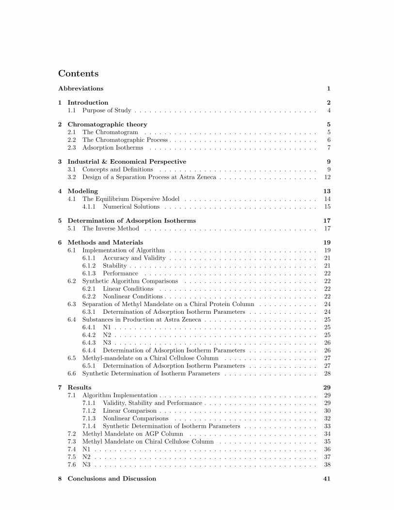
Contents

Abbreviations 1

1 Introduction 21.1 Purpose of Study . . . . . . . . . . . . . . . . . . . . . . . . . . . . . . . . . . . . . 4

2 Chromatographic theory 52.1 The Chromatogram . . . . . . . . . . . . . . . . . . . . . . . . . . . . . . . . . . . 52.2 The Chromatographic Process . . . . . . . . . . . . . . . . . . . . . . . . . . . . . . 62.3 Adsorption Isotherms . . . . . . . . . . . . . . . . . . . . . . . . . . . . . . . . . . 7

3 Industrial & Economical Perspective 93.1 Concepts and Definitions . . . . . . . . . . . . . . . . . . . . . . . . . . . . . . . . 93.2 Design of a Separation Process at Astra Zeneca . . . . . . . . . . . . . . . . . . . . 12

4 Modeling 134.1 The Equilibrium Dispersive Model . . . . . . . . . . . . . . . . . . . . . . . . . . . 14

4.1.1 Numerical Solutions . . . . . . . . . . . . . . . . . . . . . . . . . . . . . . . 15

5 Determination of Adsorption Isotherms 175.1 The Inverse Method . . . . . . . . . . . . . . . . . . . . . . . . . . . . . . . . . . . 17

6 Methods and Materials 196.1 Implementation of Algorithm . . . . . . . . . . . . . . . . . . . . . . . . . . . . . . 19

6.1.1 Accuracy and Validity . . . . . . . . . . . . . . . . . . . . . . . . . . . . . . 216.1.2 Stability . . . . . . . . . . . . . . . . . . . . . . . . . . . . . . . . . . . . . . 216.1.3 Performance . . . . . . . . . . . . . . . . . . . . . . . . . . . . . . . . . . . 22

6.2 Synthetic Algorithm Comparisons . . . . . . . . . . . . . . . . . . . . . . . . . . . 226.2.1 Linear Conditions . . . . . . . . . . . . . . . . . . . . . . . . . . . . . . . . 226.2.2 Nonlinear Conditions . . . . . . . . . . . . . . . . . . . . . . . . . . . . . . . 22

6.3 Separation of Methyl Mandelate on a Chiral Protein Column . . . . . . . . . . . . 246.3.1 Determination of Adsorption Isotherm Parameters . . . . . . . . . . . . . . 24

6.4 Substances in Production at Astra Zeneca . . . . . . . . . . . . . . . . . . . . . . . 256.4.1 N1 . . . . . . . . . . . . . . . . . . . . . . . . . . . . . . . . . . . . . . . . . 256.4.2 N2 . . . . . . . . . . . . . . . . . . . . . . . . . . . . . . . . . . . . . . . . . 256.4.3 N3 . . . . . . . . . . . . . . . . . . . . . . . . . . . . . . . . . . . . . . . . . 266.4.4 Determination of Adsorption Isotherm Parameters . . . . . . . . . . . . . . 26

6.5 Methyl-mandelate on a Chiral Cellulose Column . . . . . . . . . . . . . . . . . . . 276.5.1 Determination of Adsorption Isotherm Parameters . . . . . . . . . . . . . . 27

6.6 Synthetic Determination of Isotherm Parameters . . . . . . . . . . . . . . . . . . . 28

7 Results 297.1 Algorithm Implementation . . . . . . . . . . . . . . . . . . . . . . . . . . . . . . . . 29

7.1.1 Validity, Stability and Performance . . . . . . . . . . . . . . . . . . . . . . . 297.1.2 Linear Comparison . . . . . . . . . . . . . . . . . . . . . . . . . . . . . . . . 307.1.3 Nonlinear Comparisons . . . . . . . . . . . . . . . . . . . . . . . . . . . . . 327.1.4 Synthetic Determination of Isotherm Parameters . . . . . . . . . . . . . . . 33

7.2 Methyl Mandelate on AGP Column . . . . . . . . . . . . . . . . . . . . . . . . . . 347.3 Methyl Mandelate on Chiral Cellulose Column . . . . . . . . . . . . . . . . . . . . 357.4 N1 . . . . . . . . . . . . . . . . . . . . . . . . . . . . . . . . . . . . . . . . . . . . . 367.5 N2 . . . . . . . . . . . . . . . . . . . . . . . . . . . . . . . . . . . . . . . . . . . . . 377.6 N3 . . . . . . . . . . . . . . . . . . . . . . . . . . . . . . . . . . . . . . . . . . . . . 38

8 Conclusions and Discussion 41

9 Acknowledgements 42

References 43

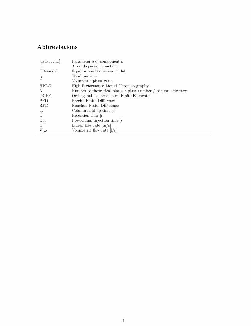
Abbreviations

[a1a2 . . . an] Parameter a of component nDa Axial dispersion constantED-model Equilibrium-Dispersive modelεt Total porosityF Volumetric phase ratioHPLC High Performance Liquid ChromatographyN Number of theoretical plates / plate number / column efficiencyOCFE Orthogonal Collocation on Finite ElementsPFD Precise Finite DifferenceRFD Rouchon Finite Differencet0 Column hold up time [s]tr Retention time [s]tsys Pre-column injection time [s]u Linear flow rate [m/s]Vvol Volumetric flow rate [l/s]

1

1 Introduction

Liquid chromatography (LC) is a conceptually straight-forward chemical separation method, yetmany of its possible modes of application can be considerably complex [Schmidt-Traub, 2005].A classical definition of the technique is:

”A separation process that is achieved by the distribution of the substances to be separated betweentwo phases, a stationary phase and a mobile phase.Those solutes distributed preferentially in the mobile phase, will move more rapidly through thesystem than those distributed preferentially in the stationary phase. Thus, the solutes will elute inorder of their increasing distribution coefficients with respect to the stationary phase.”[Cazes andScott, 2002]

The methods of LC was initially published in 1903 by the Russian botanist M.S Tswett. In hisground breaking article he describes separation of α- and β-carotenes (solutes) by using inulin(plant fibres) as stationary phase (adsorbent) and a ligroin (a petroleum distillation product) aseluent (mobile phase) [Guiochon et al., 2006].

The works made by Tswett were per definition in the realm of preparative chromatography, wherethe focus is collection of solutes rather than characterization of them as is the case in analyticalchromatography. Nevertheless, chromatography matured as an analytical technique. The initialdevelopment and realization of Twsett’s technique went rather slow and it wasn’t until the 1940’re-discovery’ rapid development in techniques and theory took place. By the late 1960’s, pumpedflow High Performance LC (HPLC) using column packed with small particles, coupled to UVdetection became available, essentially the basics of todays technology. [Cox, 2005]

The notion of different adsorption-desorption equilibrium as the ”driving force” behind separationhas been known for at least a century, yet a general theory enabling predictable modeling hasnot been found. However, many applicable models have been found and are today employed withgreat success [Guiochon et al., 2006]. All kinds of applications of chromatography can benefit frominsights drawn from simulations using these models.

Common for the mass balance equations of these mathematical models of chromatography is thelack of analytical solutions. This has necessitated the development of numerical solutions.

This project will focus on the applications of non-linear1 chromatography where the purpose is tocollect eluted components.

In an industrial viewpoint, modeling and numerical simulation of production processes should be avery interesting approach compared a traditional, empirical approach in order to better undstandthe process. Because the experimental space that can be spanned by synthetic experiments vastlyexpands that of the empirical ”trial-and-error” approach, in order to seek to optimize factors suchas purity, productivity, eluent consumption, production rate etc., there is a great economical po-tential.

Numerical solutions of any mathematical model, particularly based on partial differential equa-tions should when applied converge to the true, analytical solution and hence accurately describethe physical meaning of the model as long as it is valid.

The work as measured by CPU-time needed to converge to this true solution may grow exponen-tially and as CPU-capacity is finite, one must also consider the calculation time, but at the sametime bearing in mind that CPU-time is cheap compared to that of manual labour.

1Terms such as ”non-linear”, ”overloaded” and ”preparative” will be used interchangeably throughout this paper

2

In the end, from an industrial viewpoint, the total time from development of a process to theexecution/delivery is the most important, regardless of which method is applied.

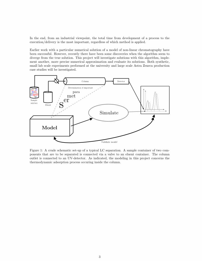
Earlier work with a particular numerical solution of a model of non-linear chromatography havebeen successful. However, recently there have been some discoveries when the algorithm seem todiverge from the true solution. This project will investigate solutions with this algorithm, imple-ment another, more precise numerical approximation and evaluate its solutions. Both synthetic,small lab scale experiments performed at the university and large scale Astra Zeneca productioncase studies will be investigated.

Figure 1: A crude schematic set-up of a typical LC separation. A sample container of two com-ponents that are to be separated is connected via a valve to an eluent container. The columnoutlet is connected to an UV-detector. As indicated, the modeling in this project concerns thethermodynamic adsorption process occuring inside the column.

3

1.1 Purpose of Study

• Study and understand the Equilibrium-Dispersive (ED) model of chromatography. Brieflystudy analytical solutions but focus on numerical solutions of non-linear chromatography.

• Study the current implementation of simulation of 2-components only, obeying the two-component competitive Bi-Langmuir model in a separation process governed by the ED-model.

• Expand and rewrite the entire current implementation to adapt for simulations of theN-component problem obeying the n-component competitive Langmuir and Bi-Langmuirmodel. Construct a MATLAB text-based user-interface and and Fortran implementation ofthe actual PDE solver.

• If programming is successful, try to port the proprietary MATLAB-MEX(-FORTRAN) im-plementation to an free software solution of Octave-Fortran.

• Implement the algorithm as a solver in the current implementation of the inverse methodalgorithm for determination of adsorption isotherm parameters.

• Use the inverse solver to determine parameters from i) performed experiments at UU andAZ ii) synthetic data generated by both methods.

• Participate in a real production at Astra Zeneca, using the modeling approach in small scalecolumns then scaling up and performing the actual separation.

• Obtain experimental data from earlier Astra Zeneca productions or potential productionsand use the new algorithm in concordance with the inverse solver algorithm to compare theoptimized adsorption isotherm parameters. Furthermore, try to exemplify and quantify themeaning of any difference in the obtained parameters. A concrete application would be theaccuracy in determining the cut point in a large-scale production process.

• Design/replicate and perform at least one practical experiment to i) gain insight and ex-perience chromatography to alleviate any possible unnecessary future puzzlements whenperforming simulations ii) determine isotherm parameters for validation of the implementedalgorithm.

• Benchmark the implementation to validate accuracy and stability. Perform synthetic studiescomparing the earlier implementation of numerical solver of the ED-model. Try to draw con-clusions about when obtained solutions diverge and the potential consequences for modeling

• Obtain reference solutions to the PDE by method considered most accurate, the orthogonalcollocation on finite element (OCFE) method.

• For the special interest of Astra Zeneca PR&D, try to i) motivate the use of simulationsin the first place, ii) motivate the use of the inverse solver for determination of adsorptionisotherm parameters iii) attract the attention and questioning the solutions obtained withRFD at low column efficiency.

4

2 Chromatographic theory

2.1 The Chromatogram

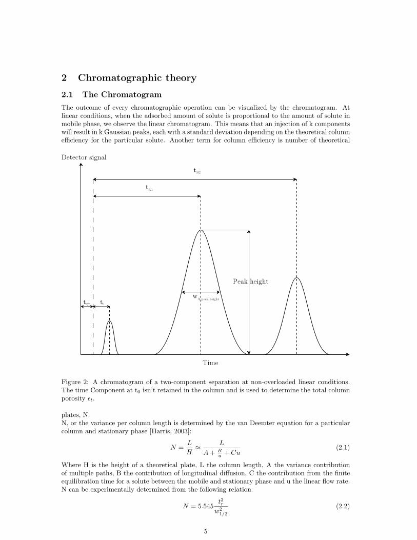
The outcome of every chromatographic operation can be visualized by the chromatogram. Atlinear conditions, when the adsorbed amount of solute is proportional to the amount of solute inmobile phase, we observe the linear chromatogram. This means that an injection of k componentswill result in k Gaussian peaks, each with a standard deviation depending on the theoretical columnefficiency for the particular solute. Another term for column efficiency is number of theoretical

Figure 2: A chromatogram of a two-component separation at non-overloaded linear conditions.The time Component at t0 isn’t retained in the column and is used to determine the total columnporosity εt.

plates, N.N, or the variance per column length is determined by the van Deemter equation for a particularcolumn and stationary phase [Harris, 2003]:

N =L

H≈ L

A+ Bu + Cu

(2.1)

Where H is the height of a theoretical plate, L the column length, A the variance contributionof multiple paths, B the contribution of longitudinal diffusion, C the contribution from the finiteequilibration time for a solute between the mobile and stationary phase and u the linear flow rate.N can be experimentally determined from the following relation.

N = 5.545t2rw2

1/2

(2.2)

5

Where tr is the retention time of a Gaussian peak, w1/2 the width of half peak maximum of thesame Gaussian peak (See Fig. 2).

A factor which affects N is the column total porosity εt. It’s defined as the ratio between the totalvolume in which solutes can traverse the column to the geometrical volume of the column.As εt increases, so does N. Because decreasing N increases the variance of the Gaussian peak (SeeFig. 2) it simultaneously decreases the chromatographic resolution Rs. This is a measure of howwell two peaks are separated.

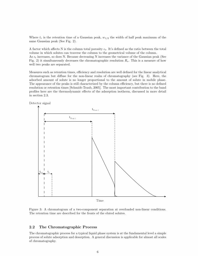
Measures such as retention times, efficiency and resolution are well defined for the linear analyticalchromatogram but diffuse for the non-linear realm of chromatography (see Fig. 3). Here, theadsorbed amount of solute is no longer proportional to the amount of solute in mobile phase.The appearance of the peaks is still characterized by the column efficiency, but there is no definedresolution or retention times [Schmidt-Traub, 2005]. The most important contribution to the bandprofiles here are the thermodynamic effects of the adsorption isotherm, discussed in more detailin section 2.3.

Figure 3: A chromatogram of a two-component separation at overloaded non-linear conditions.The retention time are described for the fronts of the eluted solutes.

2.2 The Chromatographic Process

The chromatographic process for a typical liquid phase system is at the fundamental level a simpleprocess of solute adsorption and desorption. A general discussion is applicable for almost all scalesof chromatography.

6

A column is packed with a suitable stationary phase. This is often beads with different chemicalcomposition. It could be inorganic such as active carbon, zeolites, silica or alumina or organicsuch as cross-linked organic polymers (cellulose, peptides or proteins). [Schmidt-Traub, 2005].Depending on the sought column efficiency N , column dimensions, flow rate etc, the diameter ofthe beads are chosen appropriately. Based on the nature of adsorbent, the solubility of the solutesan appropriate mobile phase is chosen. It can be a simple composition of organic or inorganicsolvents or a more complex composition.

A typical separation process2 begins with the column being equilibrated under constant temper-ature with solvent also kept at constant temperature. The outlet of the column is continuouslymonitored typically for stable UV-absorbance.

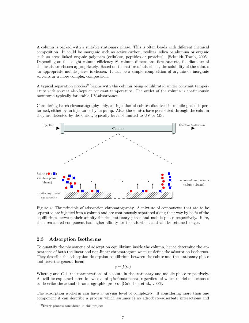
Considering batch-chromatography only, an injection of solutes dissolved in mobile phase is per-formed, either by an injector or by an pump. After the solutes have percolated through the columnthey are detected by the outlet, typically but not limited to UV or MS.

Figure 4: The principle of adsorption chromatography. A mixture of components that are to beseparated are injected into a column and are continuously separated along their way by basis of theequilibrium between their affinity for the stationary phase and mobile phase respectively. Here,the circular red component has higher affinity for the adsorbent and will be retained longer.

2.3 Adsorption Isotherms

To quantify the phenomena of adsorption equilibrium inside the column, hence determine the ap-pearance of both the linear and non-linear chromatogram we must define the adsorption isotherms.They describe the adsorption-desorption equilibrium between the solute and the stationary phaseand have the general form:

q = f(C)

Where q and C is the concentrations of a solute in the stationary and mobile phase respectively.As will be explained later, knowledge of q is fundamental regardless of which model one choosesto describe the actual chromatographic process [Guiochon et al., 2006].

The adsorption isotherm can have a varying level of complexity. If considering more than onecomponent it can describe a process which assumes i) no adsorbate-adsorbate interactions and

2Every process considered in this project

7

only one adsorbate-adsorbent interaction ii) no adsorbate-adsorbate interactions but with morethan one adsorbate-adsorbent interaction iii) adsorbate-adsorbate interactions exists but only oneadsorbent-adsorbent interaction iv) adsorbate-adsorbent interactions with many adsorbate-sorbentinteractions. In this project I will predominantly use isotherms of type i and ii.

Lets begin with breaking down the most simple case of them all, an adsorption isotherm of type iof a single component injected onto a column:

q = f(C) =αC

1± βC

At linear chromatography we observe:

limC→0

αC

1± βC= αC

At non-linear chromatography we will observe either a convex (1 + βC) or concave (1− βC) typeadsorption isotherm. The convex variant is the very common Langmuir adsorption isotherm.

Lets expand the previous discussion to two component, which doesn’t interact with each otherbut compete to adsorb to the sorbent, that is still type i.

q1 = f(C1, C2) =α1C1

1± β1C1 ± β2C2

q2 = f(C2, C1) =α2C2

1± β1C1 ± β2C2

The generalization into the k component competitive Langmuir adsorption isotherm as used inthis work.

qi =aiCi

1 +∑kj=1 bjCj

(2.3)

A typical adsorption behaviour often observed when separating chiral substances on chiral adsor-bents is that we have two interaction sites, one corresponding to the chiral interaction, unique foreach enantiomer, and another corresponding to the non-chiral interaction, common of both enan-tiomers. The simplest adsorption isotherm describing this kind of behaviour is the Bi-Langmuirisotherm which simply describes the sum of the two interactions with Langmuir terms. A greatexample of a case when this model is appropriate is the separation of the β-blocker propranolol[Fornstedt et al., 1999]

qi =a1,iCi

1 +∑nj=1 b1,jCj

+a2,iCi

1 +∑nj=1 b2,jCj

(2.4)

A more complex model which takes into account solute-solute interactions and multiple adsorbent-sorbent interactions is quadratic or statistical isotherm model3, here described for the binary case:

q1 =b1C1 + b3C1C2 + 2b4C2

1

1 + b1C1 + b2C2 + b3C1C2 + b4C21 + b5C2

2

(2.5)

q2 =b2C2 + b3C1C2 + 2b5C2

2

1 + b1C1 + b2C2 + b3C1C2 + b4C21 + b5C2

2

(2.6)

3A ratio of two polynomials which is more of strict mathematical nature than physical, since coefficents lackphysical meaning.

8

3 Industrial & Economical Perspective

One could ask one self which is the main driving force behind the study of the fundamentals ofnon-linear chromatography. Curiosity most of you might argue, minimizing the cost of productionby optimizing the separation process variables others might hastily interject [Guiochon et al., 2006].

Regardlessly, it is a fact that for example the Food and Drug Administration (FDA) has putpressure on for example the pharmaceutical industry about using process control not based onempirical observation (trial-and-error) but instead knowledge about the physio-chemical nature ofthe processes [Guiochon et al., 2006].

The scope of this section is to introduce concepts drawn from the chromatographic process, thechromatogram and briefly the economics to be able to communicate with any one involved inmanaging, designing or executing a chromatographic process. The section will only considersequential column injections i.e. batch chromatography.

3.1 Concepts and Definitions

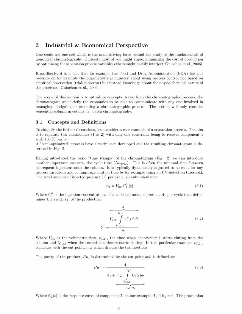
To simplify the further discussions, lets consider a case example of a separation process. The aimis to separate two enantiomers (1 & 2) with only one constraint being to recover component 1with 100 % purity.A ”semi-optimized” process have already been developed and the resulting chromatogram is de-scribed in Fig. 5.

Having introduced the basic ”time stamps” of the chromatogram (Fig. 2) we can introduceanother important measure, the cycle time (∆tcycle). This is often the minimal time betweensubsequent injections onto the column. It is typically dynamically adjusted to account for anyprocess variations and column regeneration time by for example using an UV-detection threshold.The total amount of injected product (1) per cycle is easily calculated:

n1 = VinjC01 [g] (3.1)

Where C01 is the injection concentration. The collected amount product A1 per cycle then deter-

mines the yield, Y1, of the production:

Y1 =

A1︷ ︸︸ ︷Vvol

tC,2,1∫tC,1,1

C1(t)dt

n1

(3.2)

Where Vvol is the volumetric flow, tC,1,1 the time when enantiomer 1 starts eluting from thecolumn and tC,2,1 when the second enantiomer starts eluting. In this particular example, tC,2,1coincides with the cut point, tcut which divides the two fractions.

The purity of the product, Pu1 is determined by the cut point and is defined as:

Pu1 =A1

A1 + Vvol

tcut∫tC,1,1

C2(t)dt

︸ ︷︷ ︸A1∩B1

(3.3)

Where C2(t) is the response curve of component 2. In our example A1 ∩B1 = 0. The production

9

Time [min]

Con

cent

ration

[g/l

]

C1(t)

C2(t)

tC,1,2 tC,2,2

tcycle

A1

tC,1,1

A2 ∩ B1

A2 B1

tcuttC,2,1

0 1 2 3 4 5 6 7 80

1

2

3

4

5

6

7

8

Figure 5: A fictional semi-optimized process chromatogram describing the separation of two enan-tiomers. Each is described by its response curve C1 and C2 which have been derived by simulations.The peaks are defined by the time they start eluting tC,n,1 and the time they have eluted tC,n,2.The cut point, tcut separates the fraction containing product, A1 from waste, A2 and B1.

rate Pr of component 1 and the specific production SPr can then be defined:

Pr1 =n1Y1

∆tcycle[g/min]

SPr1 =VvolPr1

[l/g](3.4)

Having made these definitions, its possible to quantify the search for the optimal separation pro-cess. The basic problem is to determine the individual band profiles C1 and C2 as functions ofthe decision variables.These variables are the parameters available to change during an optimization process, typicallybut not necessarily or limited to the column dimensions and saturation capacity, total porosity,feed concentration and injection volume and flow rate. A very common constraint is the purity ofthe collected product.

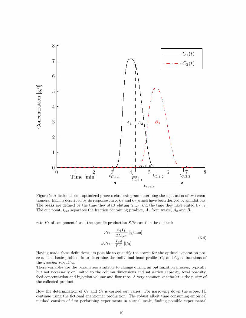
How the determination of C1 and C2 is carried out varies. For narrowing down the scope, I’llcontinue using the fictional enantiomer production. The robust albeit time consuming empiricalmethod consists of first performing experiments in a small scale, finding possible experimental

10

tcut [min]

%

PurityYield

3.5 4 4.5 5 5.5 6 6.50

10

20

30

40

50

60

70

80

90

100

Figure 6: A graph of purity and yield as functions of the cut-point tcut for the example chro-matogram in figure 5.

conditions which includes stationary and mobile phase. Then, the process is scaled up, experi-mental injections are performed and evaluated. To investigate the momentanous composition atthe outlet at different time points, fractions are collected and analyzed. After fine-tuning of of theseparation and ensuring reproducible injections, the separation process can commence. Continu-ous samples can be taken from the product fraction ensuring a stable production.

In this project I will briefly investigate the numerical approach to process optimization. Section 4will introduce chromatographic modeling, here it suffice to state that C1(t) and C2(t) are solutionsof mathematical models of the chromatographic separation process.

Still, using this numerical approach, possible experimental conditions must be empirically found.Once they have been found, a couple of suitable injections of scalable injection concentrationsshould be made. From these experimental profiles, the inverse method of finding a possible ad-sorption isotherm and its parameters is employed.

Now it’s possible to model the scale up the separation by changing column dimensions and effi-ciency and evaluating the results. The outcome from these simulations can serve as a guideline forwhere cut-points should be set. In the actual production, the cut point needs to be dynamicallyadjusted depending on the process.After finding the parameters, the experimental space which is set up is only limited to the currentstationary and the maximal injection concentration. All other decision variables such as injection

11

concentrations and volumes and flow rate can be varied and the outcome determined by simula-tions.

Each member of the set of all possible outcomes will determine the value of the objective functionused in the optimization process. Commonly used objective functions are the production rateand specific production (Eq. 3.4). Another useful function is the productivity, which states theamount of product produced per amount stationary phase per day. [Cox, 2005]

Pt1 =n1Y1

mstat24

tcycle

[g/g/day] (3.5)

Where mstat is the amount of stationary phase used in production. It may be obvious from atechnical viewpoint which of these objective functions should be maximized or minimized, butuncertain if the total cost of the production is minimized when doing so. In fact, technical andeconomical optima seldom coincides [Guiochon et al., 2006].

A unit price of an arbitrary purification can be defined:

Price =PrC

Pr1=FiC +OpC + FeC

Pr1[$/g/day] (3.6)

Where PrC is the total production cost, Pr1 the production rate, FiC fixed costs such as facilities,equipment and labour cost. OpC is the operating cost, which includes solvent, solvent recovery,waste management, energy consumption etc. FeC is the feed cost which is inversely proportionalto the yield. The higher the yield, the less lost feed, the less the feed cost. The task of minimizingthe price, a multidimensional nonlinear optimization problem will not be further discussed here.However, the general insight is that one must balance the two objective functions of productionrate and specific production, considering constraints such as yield which can lower the FeC andother requirements such as purity.

3.2 Design of a Separation Process at Astra Zeneca

The Chromatography Team at the division for PRD constantly receives substances, often phar-maceutical intermediates which needs to be purified to for example continued synthesis.Detailed knowledge of molecular structure of product and major contaminants are given, allowingresearch engineers to design a separation process.

Once suitable separation conditions have been found, the process is readily scaled up to productionscale. Here, test injections are made and fractions carefully collected during the elution. Thesefractions are analyzed for example purity and yield. Based on the findings, a cut point is set toseparate product from waste. This cutpoint is set dynamically by using a certain UV threshold.The growing product and waste fractions are also continuously monitored to ensure a stable pro-duction.Whenever a process is completed, it is always tried to recycle used solvents.

The most recent development is to use numerical determination of adsorption isotherm parametersfrom small scale experiments and then simulating the large scale production process for rapiddetermination of fraction cut-points. This approach was successfully employed in production N1,see section 6.4.1.

12

4 Modeling

Accurately describing the relation between the sum of all physical processes, retaining and dispers-ing a given component throughout its migration through the column and the chromatogram, iscrucial for several reasons. There is the the industrial, academical and ”personal understanding”perspective [Schmidt-Traub, 2005].

If chromatography is used in a larger process, a purely empirical approach in finding the optimalcontrollable process parameters can be both time consuming, maybe impossible and also expen-sive. A model which takes into account some or all of the process parameters and which canbe analytically or numerically solved can render many experiments unnecessary. The process ofmodeling in it self and its applications can lead to an increase in the understanding of the chro-matographic process and also serve as a pedagogical tool for students and people who wish to gaina better understanding of chromatography.

Many models of chromatography have been derived with varying complexity and assumptionsmade. [Guiochon et al., 2006; Schmidt-Traub, 2005]. They can be classified in four families ofmodels: The linear and ideal, the linear and non ideal, the nonlinear and ideal and the nonlinearand non ideal models [Guiochon and Lin, 2003]. The model implemented in this study is a non-linear and non ideal model.Each of the models generally take into account phenomena such as convection, dispersion, differenttype of diffusion and adsorption equilibrium or adsorption kinetics.

The basic equation of any4 model is the differential mass balance equation.

∂C

∂t+ F

∂q

∂t+ u

∂C

∂x= DL

∂2C

∂x2(4.1)

This equation describes the difference between the influx and outflux of a compound consideringan infinitesimally thin slice dx during an infinitesimally short time dt. C is the mobile phaseconcentration of the compound, q is the stationary phase concentration of the compound, F is thephase ratio, DL the axial dispersion coefficient.

The second fundamental part of any model is the adsorption behavior of a component, which isdescribed by the adsorption isotherm q. As described earlier, it suffices to state:

q = f(C) (4.2)

To state a solution to 4.1, initial and boundary conditions must be considered. In this project andtypically in most elution chromatography [Guiochon et al., 2006] the mobile phase doesn’t containany of the components one wish to separate, hence the following initial condition:

C(x, 0) = q(x, 0) = 0 (4.3)

The boundary conditions most often assumed in simulations is the rectangular pulse injection. Foran injection time of tinj and a pulse concentration C0 the left, and the unrelated right boundarycondition can be described:

C(0, t) = 0 t < 0C(0, t) = C0 0 < t ≤ tinjC(0, t) = 0 tinj < t(

∂C

∂x

)x=L

= 0

(4.4)

4This equation assumes fast mass mass transfer and simple kinetics. Other more complex mass balance equationsexists, for example the mass balance equation of the pore model [Guiochon and Lin, 2003]

13

4.1 The Equilibrium Dispersive Model

The Equilibrium-Dispersive (ED) model is a generally accepted and frequently used model ofHPLC. [Guiochon et al., 2006; Guiochon and Lin, 2003; Schmidt-Traub, 2005; Arnell, 2006]. De-spite its many simplifications of the chromatographic process, it has been successfully employedin modeling the separation of many substances.

∂Ci(x, t)∂t

+ F∂qi(x, t)∂t

+ u∂Ci(x, t)

∂x= Da,i

∂2Ci(x, t)∂x2

0 ≤ x ≤ L, t ≥ 0, i = 1, . . . n,

Ci(x, 0) = C0,i,

∂Ci(L, 0)∂x

= 0,

Ci(0, t) = φi(t)

(4.5)

F =VsV0

=1− εtεt

Da,i =Lu

2Ni

(4.6)

Equation 4.5 is written for component i. For the n-component problem, there will be n equations4.5 which needs to be solved simultaneously.Ci and qi are the mobile and stationary phase concentration respectively. F is the phase ratio,that is the quotient between the stationary phase volume and mobile phase volume.Da,i is the apparent dispersion constant which is dependent on the length L, volumetric flow ofthe mobile phase, u and the column efficiency N of a component in the column.φi(t) is the left boundary condition, that is a concentration profile of the injected sample(s). (SeeFig. 7 on page 15 for details)

The assumptions of the model are numerous. Below is a list of major assumptions [Guiochonet al., 2006].

• Since the only independent spatial variable is related to the axial position x of the column,the column is assumed to be radially homogeneous, that is, the concentration is independentof the distance from the column axis. This is a good approximation which also can be validfor carefully packed large scale columns up to 80 cm in diameter.

• Often, and in this project, the mass balance equation of the mobile phase is neglected. Thisapproximation is obviously only valid if the mobile phase doesn’t adsorb to the stationaryphase.

• Effects such as mass transfer kinetics, the finite time kinetics of the equilibrium betweenthe sorbent and adsorbent, axial and eddy diffusion is lumped into one coefficient Da. Thiscoefficient is assumed being constant. This is a good approximation only if the viscosity ofthe samples are near that of the mobile phase which means that the diffusion doesn’t dependon the concentration.

• There exists no thermal effects during the adsorption and desorption or heating of the columndue to friction and adsorption/desorption. Also, parameters such as temperature, mobilephase flow rate, viscosity, column pressure are assumed to be constant. (It’s easy to modelnon-constant flow rate)

14

t [min]

φ(t

)[m

M]

Experimental profileRectangular/linear profileRectangular profile

0 0.2 0.4 0.6 0.8 1 1.2 1.4 1.60

20

40

60

80

100

120

Figure 7: Three different injection profiles which in decreasing order of accuracy describe the leftboundary condition of Eq. 4.5: Experimental, rectangular, rectangular/linear. The experimentalinjection profile recorded was recorded when performing experiments described in section 6.5

4.1.1 Numerical Solutions

The only analytical solutions to Eq 4.5 which exists are limited to when either case i-ii holds true.

i{n = 1q = aC

ii

n = 1Da = 0q = f(C)

This fact has necessitated the development of numerical methods to solve the general form of Eq.4.5.

Existing methods range from using different kinds of finite difference approximations to finiteelement approximations (Orthogonal Collocation of Finite Elements, OCFE). [Guiochon, 2002].OCFE is considered to be the most accurate method currently available but requires considerablecomputational time [Kaczmarski, 2007].A particular variant of the finite difference method is the ”Rouchon forward-backward scheme”[Rouchon et al., 1987]. This scheme makes some clever simplifications, drastically reducing com-putational time and has been used in many applications as solver of Eq. 4.5 [Samuelsson, 2008;Arnell, 2006; Forssen, 2005].

15

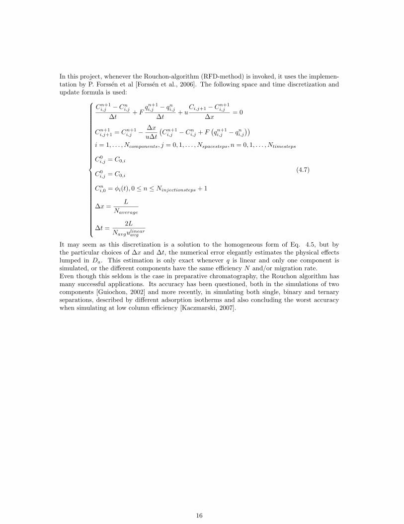
In this project, whenever the Rouchon-algorithm (RFD-method) is invoked, it uses the implemen-tation by P. Forssen et al [Forssen et al., 2006]. The following space and time discretization andupdate formula is used:

Cn+1i,j − Cni,j

∆t+ F

qn+1i,j − qni,j

∆t+ u

Ci,j+1 − Cn+1i,j

∆x= 0

Cn+1i,j+1 = Cn+1

i,j −∆xu∆t

(Cn+1i,j − C

ni,j + F

(qn+1i,j − q

ni,j

))i = 1, . . . , Ncomponents, j = 0, 1, . . . , Nspacesteps, n = 0, 1, . . . , Ntimesteps

C0i,j = C0,i

C0i,j = C0,i

Cni,0 = φi(t), 0 ≤ n ≤ Ninjectionsteps + 1

∆x =L

Naverage

∆t =2L

Navgulinearavg

(4.7)

It may seem as this discretization is a solution to the homogeneous form of Eq. 4.5, but bythe particular choices of ∆x and ∆t, the numerical error elegantly estimates the physical effectslumped in Da. This estimation is only exact whenever q is linear and only one component issimulated, or the different components have the same efficiency N and/or migration rate.Even though this seldom is the case in preparative chromatography, the Rouchon algorithm hasmany successful applications. Its accuracy has been questioned, both in the simulations of twocomponents [Guiochon, 2002] and more recently, in simulating both single, binary and ternaryseparations, described by different adsorption isotherms and also concluding the worst accuracywhen simulating at low column efficiency [Kaczmarski, 2007].

16

5 Determination of Adsorption Isotherms

Since the behavior of any chromatographic separation as modeled by Eq. 4.5 is governed by theadsorption isotherm, q = f(C), any use of this model in the purpose of designing/and or optimiz-ing a preparative chromatographic process requires the accurate determination of its parameters[Felinger et al., 2003].

As was described in section 2.3, there are a multitude of different adsorption isotherms, many ofwhich have been derived on physical basis and some of strict mathematical nature as the quadraticisotherm, coinciding with the Pade approximation [Guiochon and Lin, 2003]. While the latter mayapproximate the former, the physical meaning is lost and no further insight into the adsorptionprocess can be drawn from such an approximation.

Many experimental methods of determining adsorption isotherm parameters can only be appliedto the case of single component separation. Due to the competitive nature of adsorption equilib-rium, this data can’t be extrapolated to the case of multicomponent separation.

Examples of popular methods not dissected in this project are frontal analysis (FA), elution bycharacteristic point (ECP), FA by ECP, (FACP), injection on plateau method (PM) and the per-tubation peak method (PP) [Samuelsson, 2008].These methods have in common that one first determine the value of q, then determine f(C) suchthat q = f(C) using nonlinear regression, choosing a suitable model. Ideally, one should performthis regression against all known models, then afterwards evaluate which model has the better fit.

Currently, there is no way of knowing beforehand, given a particular solute and adsorbent, whichlevel of complexity is required, that is, which model can be used to fit experimental data [Forssenet al., 2006]. The previously mentioned methods will give the most accurate determination ofparameters.

5.1 The Inverse Method

The inverse method uses a work flow that is, as expected, opposite to that of the earlier mentionedmethods [Felinger et al., 2003]. The general approach is to perform a number (the more the better)of experiments and record the chromatograms.

The next step is to determine which differential mass balance model to use (e.g. Eq 4.5), whichtype of adsorption isotherm is applicable and then guess the start values of the isotherm. Intheory, this is a very straight-forward approach but in reality there are complications. Becausethe recorded detector response is the sum of the response from all the components present at thedetector but the simulated responses are per component, there can be problems doing a properdetector calibration if the response isn’t linear. This can be solved by using other detectionmethods than UV [Guiochon et al., 2006] and is of no problem when simulating the separationof enantiomers which have identical and linear UV-response [Forssen et al., 2006]. If separatingenantiomers, one can take two approaches: one is to create a calibration curve by injecting a seriesof know concentrations into the detector or either injecting different amounts of enantiomers intothe column, the integrating the total area of the chromatogram, hence doing the actual detectorcalibration.

The next step is to load the experimental chromatograms, superimpose the simulated chro-matograms and calculate the degree of overlap in a nonlinear least-square procedure.Then an optimization routine is started where parameters first are varied or perturbed accordingto a specific algorithm, for example a gradient based [Forssen et al., 2006] or based on a geneticalgorithm [Zhang et al., 2008]. The change in degree of overlap is noted and depending on thedirection and its magnitude, the parameters will change accordingly. The optimization routine

17

will end when some convergence criteria is reached or the algorithm can’t adjust the parametersto give a better degree of fit. As with the experimental approach mentioned earlier, one shouldtry to loop through different adsorption isotherm models and evaluate which has the best fit.

The large number of experiments and high consumption of solvent and samples needed when per-forming the classical methods of isotherm determination can be drastically reduced by the use ofthe inverse method [Forssen et al., 2006].

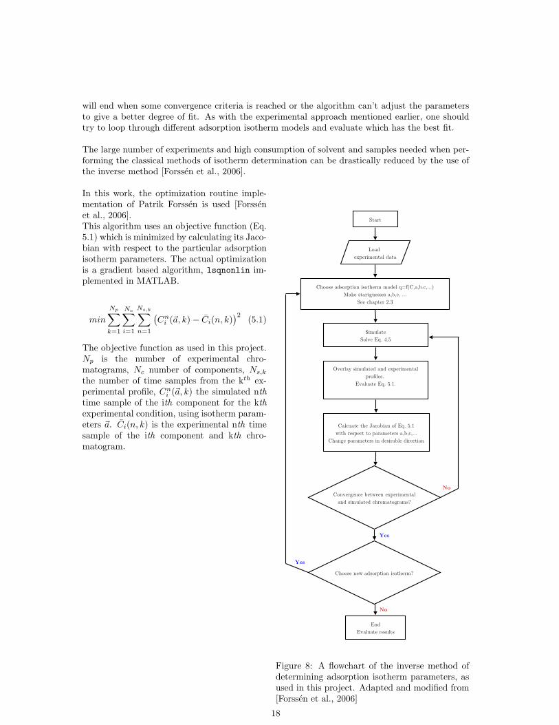
Figure 8: A flowchart of the inverse method ofdetermining adsorption isotherm parameters, asused in this project. Adapted and modified from[Forssen et al., 2006]

In this work, the optimization routine imple-mentation of Patrik Forssen is used [Forssenet al., 2006].This algorithm uses an objective function (Eq.5.1) which is minimized by calculating its Jaco-bian with respect to the particular adsorptionisotherm parameters. The actual optimizationis a gradient based algorithm, lsqnonlin im-plemented in MATLAB.

min

Np∑k=1

Nc∑i=1

Ns,k∑n=1

(Cni (~a, k)− Ci(n, k)

)2 (5.1)

The objective function as used in this project.Np is the number of experimental chro-matograms, Nc number of components, Ns,kthe number of time samples from the kth ex-perimental profile, Cni (~a, k) the simulated nthtime sample of the ith component for the kthexperimental condition, using isotherm param-eters ~a. Ci(n, k) is the experimental nth timesample of the ith component and kth chro-matogram.

18

6 Methods and Materials

6.1 Implementation of Algorithm

The problem is to find a numerical approximation to Eq. 4.5, reprinted below.

∂Ci(x, t)∂t

+ F∂qi(x, t)∂t

+ u∂Ci(x, t)

∂x= Da,i

∂2Ci(x, t)∂x2

0 ≤ x ≤ L, t ≥ 0, i = 1, . . . n,

Ci(x, 0) = C0,i,

∂Ci(L, 0)∂x

= 0,

Ci(0, t) = φi(t)

The first step is to approximate the partial derivates using ordinary finite difference quotients.This can be made in many ways [Guiochon and Lin, 2003] but in this project the followingapproximations have been used.(

∂Ci∂t

)nj

≈Cn+1i,j − Cni,j

∆t+O(∆t)

(∂Ci∂x

)nj

≈Cni,j+1 − Cni,j−1

2∆x+O(∆x2)

(∂2Ci∂x2

)nj

≈Cni,j+1 − 2Cni,j + Cni,j−1

∆x2+O(∆x2)

(6.1)

Since q = f(C) the chain rule can be applied to the partial derivative ∂qi∂t . For k components we

have:

∂qi∂t

=k∑z=1

∂qi∂Cz

∂Cz∂t

(6.2)

By substituting Eq. 6.2 and 6.1 into Eq. 4.5 we have:

Cn+1i,j − Cni,j

∆t+ F

k∑z=1

∂qi∂Cz

Cn+1z,j − Cnz,j

∆t+ u

Cni,j+1 − Cni,j−1

2∆x= Dai

Cni,j+1 − 2Cni,j + Cni,j−1

∆x2(6.3)

An explicit statement of Eq. 6.3 for two components:

(1 + F

∂q1

∂C1

)Cn+1

1,j − Cn1,j∆t

+ F∂q1

∂C2

(Cn+1

2,j − Cn2,j∆t

)+ u

Cn1,j+1 − Cn1,j−1

2∆x= Da1

Cn1,j+1 − 2Cn1,j + Cn1,j−1

∆x2(1 + F

∂q2

∂C2

)Cn+1

2,j − Cn2,j∆t

+ F∂q2

∂C1

(Cn+1

1,j − Cn1,j∆t

)+ u

Cn2,j+1 − Cn2,j−1

2∆x= Da2

Cn2,j+1 − 2Cn2,j + Cn2,j−1

∆x2

(6.4)

19

The generalization into k components leads to an equation system of k equations with k unknownson the form:

a11Cn+1

1,j −Cn1,j

∆t a12Cn+1

2,j −Cn2,j

∆t · · · a1kCn+1k,j −C

nk,j

∆t |c1a21

Cn+11,j −C

n1,j

∆t a22Cn+1

2,j −Cn2,j

∆t · · · a2kCn+1k,j −C

nk,j

∆t |c2...

.... . .

......

ak1Cn+1

1,j −Cn1,j

∆t ak2Cn+1

2,j −Cn2,j

∆t · · · akkCn+1k,j −C

nk,j

∆t |ck

(6.5)

Where the coefficients are calculated as follows:

aαβ =

{1 + F ∂qα

∂Cβα = β

F ∂qα∂Cβ

α 6= βcκ = Daκ

Cnκ,j+1 − 2Cnκ,j + Cnκ,j−1

∆x2− u

Cnκ,j+1 − Cnκ,j−1

2∆x

(6.6)

An update formula for determining the unknown variables Cn+1κ,j can be explicitly stated:

Cn+1

1,j

Cn+12,j...

Cn+1κ,j

=∆t−1

a11 a12 · · · a1k

a21 a22 · · · a2k

......

. . ....

ak1 ak2 · · · akk

−1

c1c2...cκ

+

cn1,jcn2,j

...cnκ,j

(6.7)

This update formula needs to be evaluated at every time step n for each room step j. Additionally∂qα∂Cβ

needs to updated the same number of times.

In the implementation, no matrix inversion operation is performed but the linear system of equa-tions of Eq. 6.5 is solved by using the standard solver DGESV as implemented in the LAPACK v3.2library [Anderson et al., 1999]

The stability criteria for a certain finite difference implementation of lesser accuracy [Guiochonand Lin, 2003] has been derived. It basically states that the number of room steps in which thecolumn needs to be discretized should be equal to the number of theoretical plates. This is anintuitive condition considering the definition of a theoretical plate.The second criteria on the time step is less intuitive, but it obviously depends on magnitude of thederivative of the adsorption isotherm and also the lenght of a room step. No effort has been madeto the complex task of deriving similar critiera for this particular implementation. In this project,the room step is chosen to fulfill the earlier derived criteria but the second will be empiricallydetermined and dynamically adjusted to reach stability. The definition of stability in this case isconserved mass.

The column is discretized as follows.

M =max (Ni) Number of space steps

dx =L

MLength of a space step

dt =λdx

max(L~tR

) Length of a time step

20

Where ~tR is a vector containing all the retention times of the components as derived using thecurrent adsorption isotherm (See Sec. 2.3) at infinite dilution. dt is therefore chosen as a fractionλ of the time it takes for the fastest component to traverse a space step.

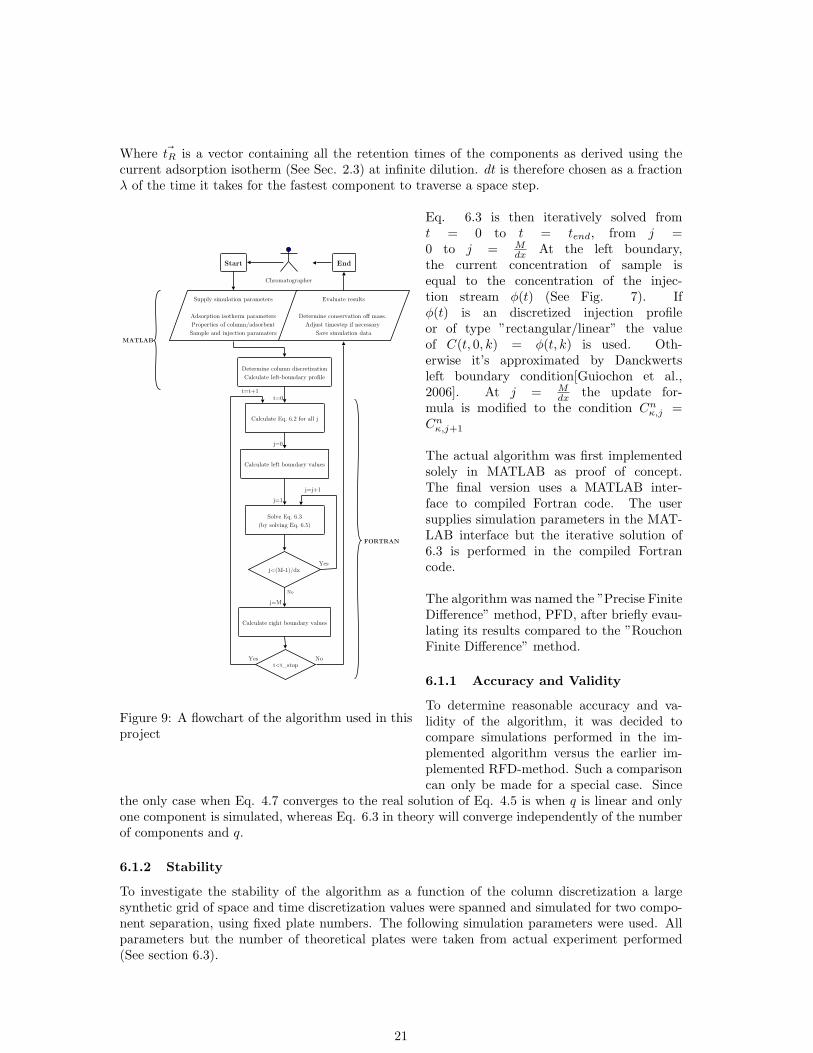
Figure 9: A flowchart of the algorithm used in thisproject

Eq. 6.3 is then iteratively solved fromt = 0 to t = tend, from j =0 to j = M

dx At the left boundary,the current concentration of sample isequal to the concentration of the injec-tion stream φ(t) (See Fig. 7). Ifφ(t) is an discretized injection profileor of type ”rectangular/linear” the valueof C(t, 0, k) = φ(t, k) is used. Oth-erwise it’s approximated by Danckwertsleft boundary condition[Guiochon et al.,2006]. At j = M

dx the update for-mula is modified to the condition Cnκ,j =Cnκ,j+1

The actual algorithm was first implementedsolely in MATLAB as proof of concept.The final version uses a MATLAB inter-face to compiled Fortran code. The usersupplies simulation parameters in the MAT-LAB interface but the iterative solution of6.3 is performed in the compiled Fortrancode.

The algorithm was named the ”Precise FiniteDifference” method, PFD, after briefly evau-lating its results compared to the ”RouchonFinite Difference” method.

6.1.1 Accuracy and Validity

To determine reasonable accuracy and va-lidity of the algorithm, it was decided tocompare simulations performed in the im-plemented algorithm versus the earlier im-plemented RFD-method. Such a comparisoncan only be made for a special case. Since

the only case when Eq. 4.7 converges to the real solution of Eq. 4.5 is when q is linear and onlyone component is simulated, whereas Eq. 6.3 in theory will converge independently of the numberof components and q.

6.1.2 Stability

To investigate the stability of the algorithm as a function of the column discretization a largesynthetic grid of space and time discretization values were spanned and simulated for two compo-nent separation, using fixed plate numbers. The following simulation parameters were used. Allparameters but the number of theoretical plates were taken from actual experiment performed(See section 6.3).

21

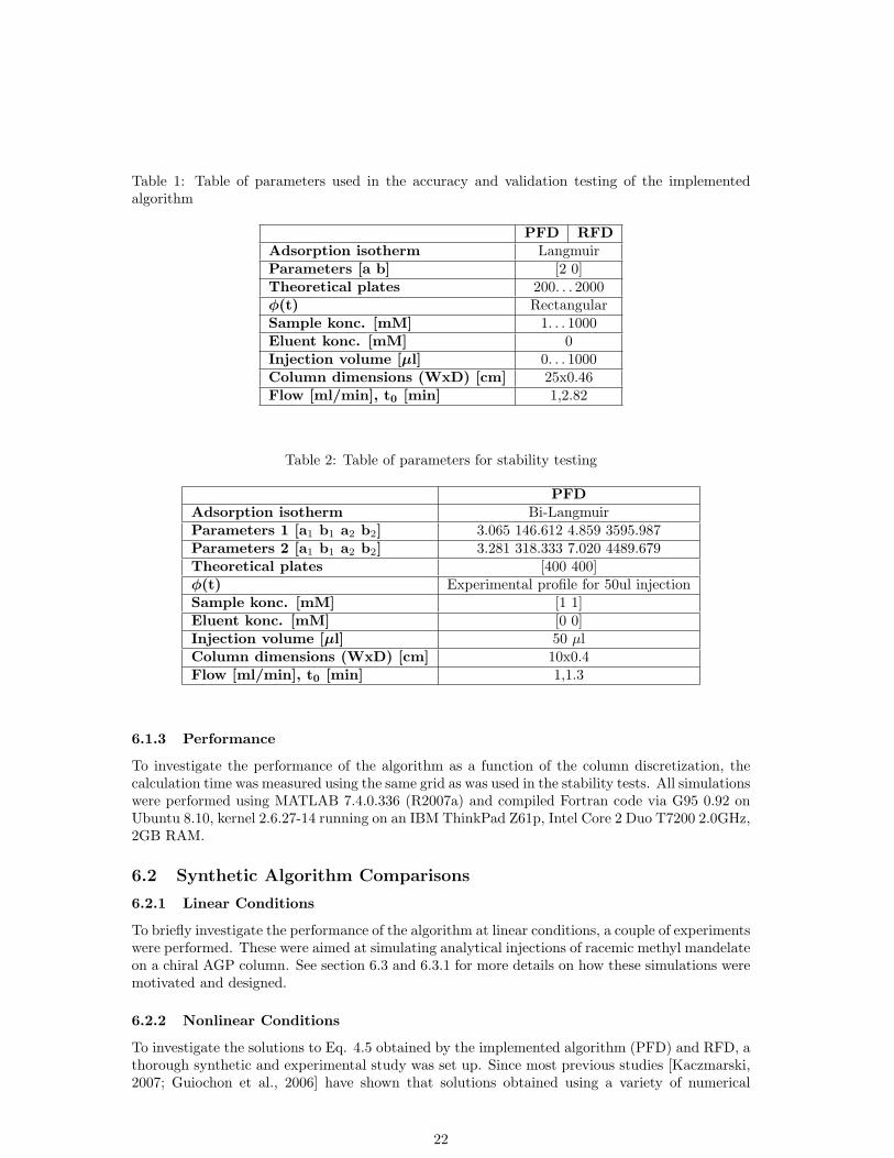
Table 1: Table of parameters used in the accuracy and validation testing of the implementedalgorithm

PFD RFDAdsorption isotherm LangmuirParameters [a b] [2 0]Theoretical plates 200. . . 2000φ(t) RectangularSample konc. [mM] 1. . . 1000Eluent konc. [mM] 0Injection volume [µl] 0. . . 1000Column dimensions (WxD) [cm] 25x0.46Flow [ml/min], t0 [min] 1,2.82

Table 2: Table of parameters for stability testing

PFDAdsorption isotherm Bi-LangmuirParameters 1 [a1 b1 a2 b2] 3.065 146.612 4.859 3595.987Parameters 2 [a1 b1 a2 b2] 3.281 318.333 7.020 4489.679Theoretical plates [400 400]φ(t) Experimental profile for 50ul injectionSample konc. [mM] [1 1]Eluent konc. [mM] [0 0]Injection volume [µl] 50 µlColumn dimensions (WxD) [cm] 10x0.4Flow [ml/min], t0 [min] 1,1.3

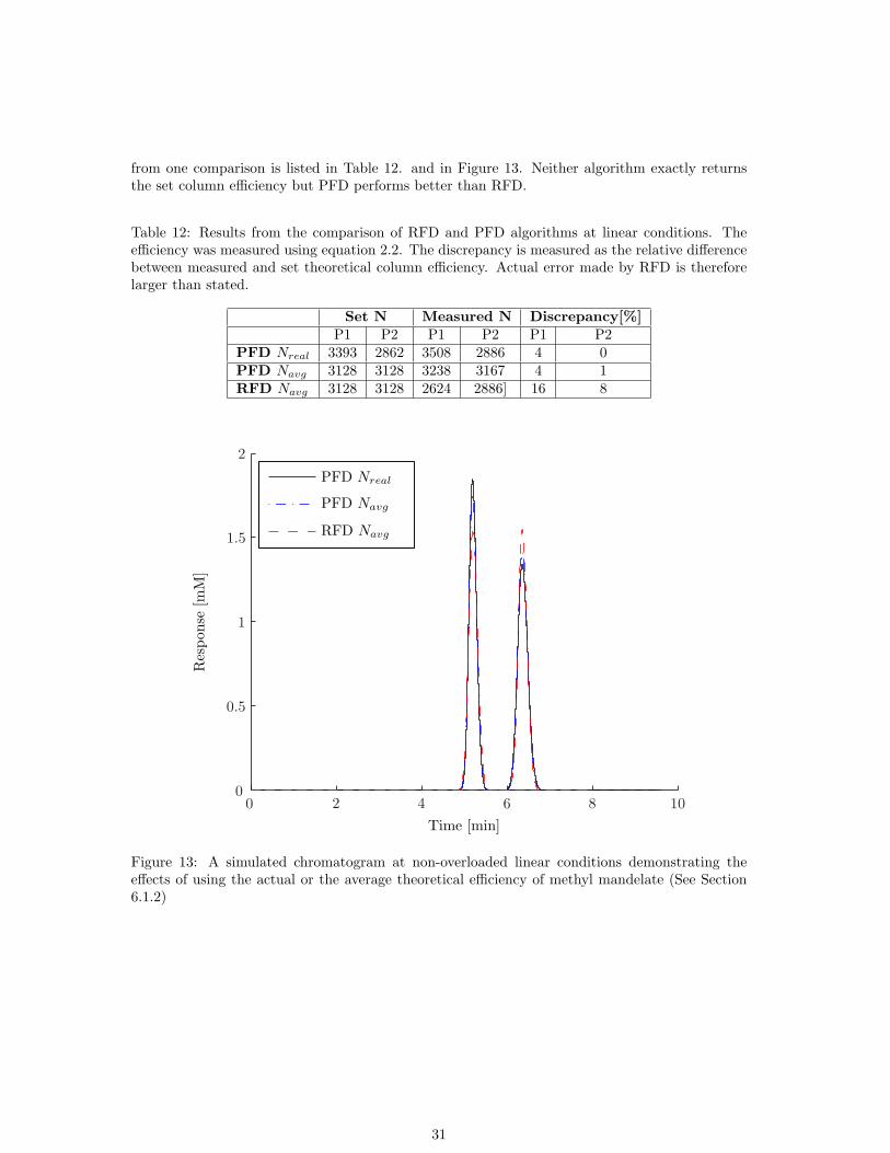
6.1.3 Performance

To investigate the performance of the algorithm as a function of the column discretization, thecalculation time was measured using the same grid as was used in the stability tests. All simulationswere performed using MATLAB 7.4.0.336 (R2007a) and compiled Fortran code via G95 0.92 onUbuntu 8.10, kernel 2.6.27-14 running on an IBM ThinkPad Z61p, Intel Core 2 Duo T7200 2.0GHz,2GB RAM.

6.2 Synthetic Algorithm Comparisons

6.2.1 Linear Conditions

To briefly investigate the performance of the algorithm at linear conditions, a couple of experimentswere performed. These were aimed at simulating analytical injections of racemic methyl mandelateon a chiral AGP column. See section 6.3 and 6.3.1 for more details on how these simulations weremotivated and designed.

6.2.2 Nonlinear Conditions

To investigate the solutions to Eq. 4.5 obtained by the implemented algorithm (PFD) and RFD, athorough synthetic and experimental study was set up. Since most previous studies [Kaczmarski,2007; Guiochon et al., 2006] have shown that solutions obtained using a variety of numerical

22

Table 3: Parameters used for the linear study comparing solutions of PFD and RFDPFD RFD

Adsorption isotherm Bi-LangmuirParameters 1 [a1 b1 a2 b2] 3.065 146.612 4.859 3595.987Parameters 2 [a1 b1 a2 b2] 3.281 318.333 7.020 4489.679Theoretical plates [3393 2862] [3128]φ(t) Rectangular/linearSample konc. [µM] [40 40]Eluent konc. [µM] [0 0]Injection volume [µl] 7Column dimensions (WxD) [cm] 10x0.4Flow [ml/min], t0 [min] 0.7,1.3

schemes markedly differ at low column efficiency, focus was directed to artificially varying thecolumn efficiency.

Because solutions obtained using the OCFE method are considered to always converge to the realsolution, it was imperative to include these solutions as well. Since no working implementation ofthe OCFE method has been implemented at the lab, all solutions that will be presented are thanksto professor Krzysztof Kaczmarski. We don’t have access to his source code but have ensured thatsimulations are performed using identical parameters and injection profiles.

In total, 72 simulations were performed using each algorithm. Due to unforeseen problems withloss of mass using the RFD algorithm and experimental injection profiles, all simulations had tobe repeated using a modified interpolated injection profile which assures conserved mass. For thecomparisons at linear and non-linear conditions, see sections 6.3 and 6.3.1 for how the simulationswere designed.

Table 4: Parameters used for the non-linear study

PFD RFD OCFEAdsorption isotherm Bi-LangmuirParameters 1 [a1 b1 a2 b2] 3.065 146.612 4.859 3595.987Parameters 2 [a1 b1 a2 b2] 3.281 318.333 7.020 4489.679Theoretical plates [3393 2862]. . . [113 95] 3127. . . 104 [3393 2862]. . . [189 159]φ(t) Interpolated experimental 50 µlSample konc. [µM] See section 6.3, table 5Eluent konc. [µM] [0 0]Injection volume [µl] 25,50,75,100Column dimensions [cm] 10x0.4Flow [ml/min], t0 [min] 0.7,1.3

23

6.3 Separation of Methyl Mandelate on a Chiral Protein Column

A 10x0.4 cm chiral AGP column (ChromTech, Hagersten, Sweden) consisting of 5µm silica beadswith immobilized α1-glycoprotein as chiral selector was was installed in a Hewlett-Packard, Agi-lent 1100 system.

Eluent was prepared by dissolving appropriate amounts of acetic acid and sodium acetate, creatingan 75 mM acetate buffer at pH 5, ionic strength 50 mM. Additionally, methanol was added to aconcentration of 1.4 % (v/v). The buffer was filtered through a 45 µm filter before use.

The column was equilibrated with eluent at a constant flow at 0.7 ml/min and kept at 20 ◦Cduring all experiments. UV-detection was made simultaneously at 6 different wavelengths but allfurther data processing used data obtained at 254 nm where the detector response was found tobe linear.

A 2mM stock solution of (+/-)-methyl mandelate was prepared by dissolving appropriate amountsof (+/-)-methyl mandelate (Sigma-Aldrich, Stockholm, Sweden) directly in the mobile phase.

A calibration curve of absorbance vs concentration was constructed by overriding the automaticinjector and manually injecting 0.5 ml of one enantiomer by a different valve bypassing the col-umn and reaching response plateaus.5. To validate the calibration, some replicates of the knownamounts of the other enantiomer were also injected.

A linear regression of the data was performed using polyfit as implemented in MATLAB R2007a(The MathWorks, Natick, USA). Experimental chromatograms were exported and processed usingthis calibration polynomial.

To measure the injection profile of the system, the capillary tube connecting the injector andcolumn was connected directly into the UV-detector whereupon a triplicate of 50 µl injections of0.5 mM (+)-methyl mandelate were made.

Initial analytical injections to determine column porosity and efficiency of the two enantiomerswere made in triplicate by injecting 7 µl 40 µM racemate and single injections of each enantiomer.A number of overloaded injections were made after experimenting with suitable injection amountsand different ratios between the enantiomers. The experiments are listed in Table 5.No void-volume marker was used.

6.3.1 Determination of Adsorption Isotherm Parameters

After performing the actual experiments all experimental chromatograms were processed and con-verted from UV-response vs time to concentration vs time. The porosity of the column wasdetermined, as was the efficiency of the both components by using equation 2.2.

The measured injection profile at 50 µl was also converted and interpolated by a piecewise polyno-mial. The polynomial was then normalized to the known concentration for which it was recorded.Thus, its possible to use this polynomial and interpolate an arbitrary injection concentration. Theoptimization employs the RFD-algorithm. The experimental profiles and parameters used for theinverse solver are listed in Table 6.3.

5The absorbance reading at the plateau corresponds to the response at the particular injection concentration

24

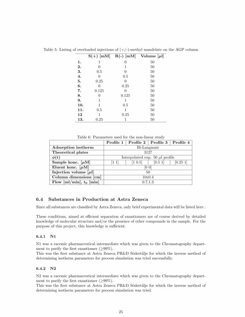
Table 5: Listing of overloaded injections of (+/-)-methyl mandelate on the AGP column

S(+) [mM] R(-) [mM] Volume [µl]1. 1 0 502. 0 1 503. 0.5 0 504. 0 0.5 505. 0.25 0 506. 0 0.25 507. 0.125 0 508. 0 0.125 509. 1 1 5010. 1 0.5 5011. 0.5 1 5012 1 0.25 5013. 0.25 1 50

Table 6: Parameters used for the non-linear studyProfile 1 Profile 2 Profile 3 Profile 4

Adsorption isotherm Bi-LangmuirTheoretical plates 3127φ(t) Interpolated exp. 50 µl profileSample konc. [µM] [1 1] [1 0.5] [0.5 1] [0.25 1]Eluent konc. [µM] [0 0]Injection volume [µl] 50Column dimensions [cm] 10x0.4Flow [ml/min], t0 [min] 0.7,1.3

6.4 Substances in Production at Astra Zeneca

Since all substances are classified by Astra Zeneca, only brief experimental data will be listed here .

These conditions, aimed at efficient separation of enantiomers are of course derived by detailedknowledge of molecular structure and/or the presence of other compounds in the sample. For thepurpose of this project, this knowledge is sufficient.

6.4.1 N1

N1 was a racemic pharmaceutical intermediate which was given to the Chromatography depart-ment to purify the first enantiomer (≥99%).This was the first substance at Astra Zeneca PR&D Sodertalje for which the inverse method ofdetermining isotherm parameters for process simulation was tried successfully.

6.4.2 N2

N2 was a racemic pharmaceutical intermediate which was given to the Chromatography depart-ment to purify the first enantiomer (≥99%).This was the first substance at Astra Zeneca PR&D Sodertalje for which the inverse method ofdetermining isotherm parameters for process simulation was tried.

25

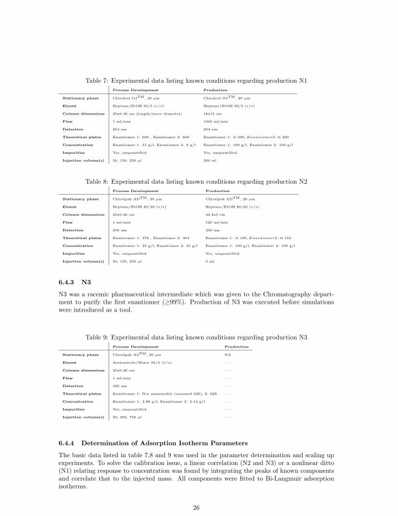
Table 7: Experimental data listing known conditions regarding production N1Process Development Production

Stationary phase Chiralcel OJTM, 20 µm Chiralcel OJTM, 20 µm

Eluent Heptane/EtOH 95/5 (v/v) Heptane/EtOH 95/5 (v/v)

Column dimensions 25x0.46 cm (length/inner diameter) 18x15 cm

Flow 1 ml/min 1000 ml/min

Detection 254 nm 254 nm

Theoretical plates Enantiomer 1: 600 , Enantiomer 2: 600 Enantiomer 1: ≈ 290, Enantiomer2 :≈ 290

Concentration Enantiomer 1: 31 g/l, Enantiomer 2: 9 g/l Enantiomer 1: 100 g/l, Enantiomer 2: 100 g/l

Impurities Yes, unquantified Yes, unquantified

Injection volume(s) 50, 150, 250 µl 200 ml

Table 8: Experimental data listing known conditions regarding production N2Process Development Production

Stationary phase Chiralpak ADTM, 20 µm Chiralpak ADTM, 20 µm

Eluent Heptane/EtOH 80/20 (v/v) Heptane/EtOH 80/20 (v/v)

Column dimensions 25x0.46 cm 42.4x5 cm

Flow 1 ml/min 120 ml/min

Detection 230 nm 230 nm

Theoretical plates Enantiomer 1: 378 , Enantiomer 2: 304 Enantiomer 1: ≈ 190, Enantiomer2 :≈ 152

Concentration Enantiomer 1: 25 g/l, Enantiomer 2: 25 g/l Enantiomer 1: 100 g/l, Enantiomer 2: 100 g/l

Impurities Yes, unquantified Yes, unquantified

Injection volume(s) 50, 150, 250 µl 5 ml

6.4.3 N3

N3 was a racemic pharmaceutical intermediate which was given to the Chromatography depart-ment to purify the first enantiomer (≥99%). Production of N3 was executed before simulationswere introduced as a tool.

Table 9: Experimental data listing known conditions regarding production N3Process Development Production

Stationary phase Chiralpak ASTM, 20 µm NA

Eluent Acetonitrile/Water 95/5 (v/v) · · ·

Column dimensions 25x0.46 cm · · ·

Flow 1 ml/min · · ·

Detection 320 nm · · ·

Theoretical plates Enantiomer 1: Not measurable (assumed 629), 2: 629 · · ·

Concentration Enantiomer 1: 2.86 g/l, Enantiomer 2: 2.14 g/l · · ·

Impurities Yes, unquantified · · ·

Injection volume(s) 50, 250, 750 µl · · ·

6.4.4 Determination of Adsorption Isotherm Parameters

The basic data listed in table 7,8 and 9 was used in the parameter determination and scaling upexperiments. To solve the calibration issue, a linear correlation (N2 and N3) or a nonlinear ditto(N1) relating response to concentration was found by integrating the peaks of known componentsand correlate that to the injected mass. All components were fitted to Bi-Langmuir adsorptionisotherms.

26

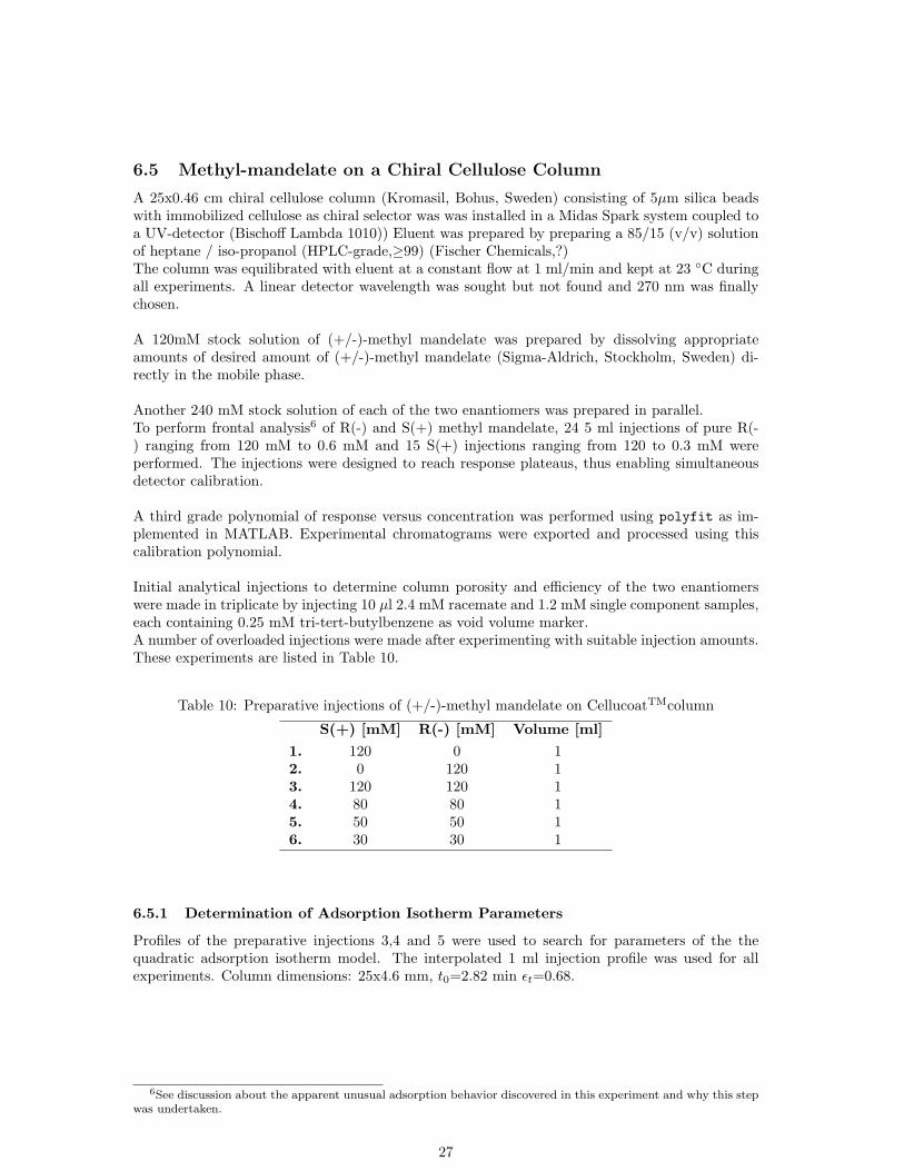
6.5 Methyl-mandelate on a Chiral Cellulose Column

A 25x0.46 cm chiral cellulose column (Kromasil, Bohus, Sweden) consisting of 5µm silica beadswith immobilized cellulose as chiral selector was was installed in a Midas Spark system coupled toa UV-detector (Bischoff Lambda 1010)) Eluent was prepared by preparing a 85/15 (v/v) solutionof heptane / iso-propanol (HPLC-grade,≥99) (Fischer Chemicals,?)The column was equilibrated with eluent at a constant flow at 1 ml/min and kept at 23 ◦C duringall experiments. A linear detector wavelength was sought but not found and 270 nm was finallychosen.

A 120mM stock solution of (+/-)-methyl mandelate was prepared by dissolving appropriateamounts of desired amount of (+/-)-methyl mandelate (Sigma-Aldrich, Stockholm, Sweden) di-rectly in the mobile phase.

Another 240 mM stock solution of each of the two enantiomers was prepared in parallel.To perform frontal analysis6 of R(-) and S(+) methyl mandelate, 24 5 ml injections of pure R(-) ranging from 120 mM to 0.6 mM and 15 S(+) injections ranging from 120 to 0.3 mM wereperformed. The injections were designed to reach response plateaus, thus enabling simultaneousdetector calibration.

A third grade polynomial of response versus concentration was performed using polyfit as im-plemented in MATLAB. Experimental chromatograms were exported and processed using thiscalibration polynomial.

Initial analytical injections to determine column porosity and efficiency of the two enantiomerswere made in triplicate by injecting 10 µl 2.4 mM racemate and 1.2 mM single component samples,each containing 0.25 mM tri-tert-butylbenzene as void volume marker.A number of overloaded injections were made after experimenting with suitable injection amounts.These experiments are listed in Table 10.

Table 10: Preparative injections of (+/-)-methyl mandelate on CellucoatTMcolumn

S(+) [mM] R(-) [mM] Volume [ml]1. 120 0 12. 0 120 13. 120 120 14. 80 80 15. 50 50 16. 30 30 1

6.5.1 Determination of Adsorption Isotherm Parameters

Profiles of the preparative injections 3,4 and 5 were used to search for parameters of the thequadratic adsorption isotherm model. The interpolated 1 ml injection profile was used for allexperiments. Column dimensions: 25x4.6 mm, t0=2.82 min εt=0.68.

6See discussion about the apparent unusual adsorption behavior discovered in this experiment and why this stepwas undertaken.

27

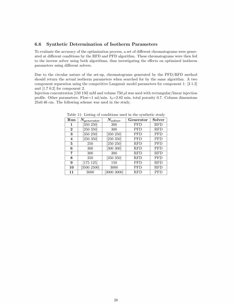
6.6 Synthetic Determination of Isotherm Parameters

To evaluate the accuracy of the optimization process, a set of different chromatograms were gener-ated at different conditions by the RFD and PFD algorithm. These chromatograms were then fedto the inverse solver using both algorithms, thus investigating the effects on optimized isothermparameters using different solvers.

Due to the circular nature of the set-up, chromatograms generated by the PFD/RFD methodshould return the actual isotherm parameters when searched for by the same algorithm. A twocomponent separation using the competitive Langmuir model parameters for component 1: [3 1.2]and [1.7 0.2] for component 2.Injection concentration [150 150] mM and volume 750 µl was used with rectangular/linear injectionprofile. Other parameters: Flow=1 ml/min. t0=2.82 min, total porosity 0.7. Column dimensions25x0.46 cm. The following scheme was used in the study.

Table 11: Listing of conditions used in the synthetic studyRun Ngenerator Nsolver Generator Solver

1 [350 250] 300 PFD RFD2 [250 350] 300 PFD RFD3 [350 250] [350 250] PFD PFD4 [250 350] [250 350] PFD PFD5 250 [250 250] RFD PFD6 300 [300 300] RFD PFD7 300 300 RFD RFD8 350 [350 350] RFD PFD9 [175 125] 150 PFD RFD10 [3500 2500] 3000 PFD RFD11 3000 [3000 3000] RFD PFD

28

7 Results

7.1 Algorithm Implementation

7.1.1 Validity, Stability and Performance

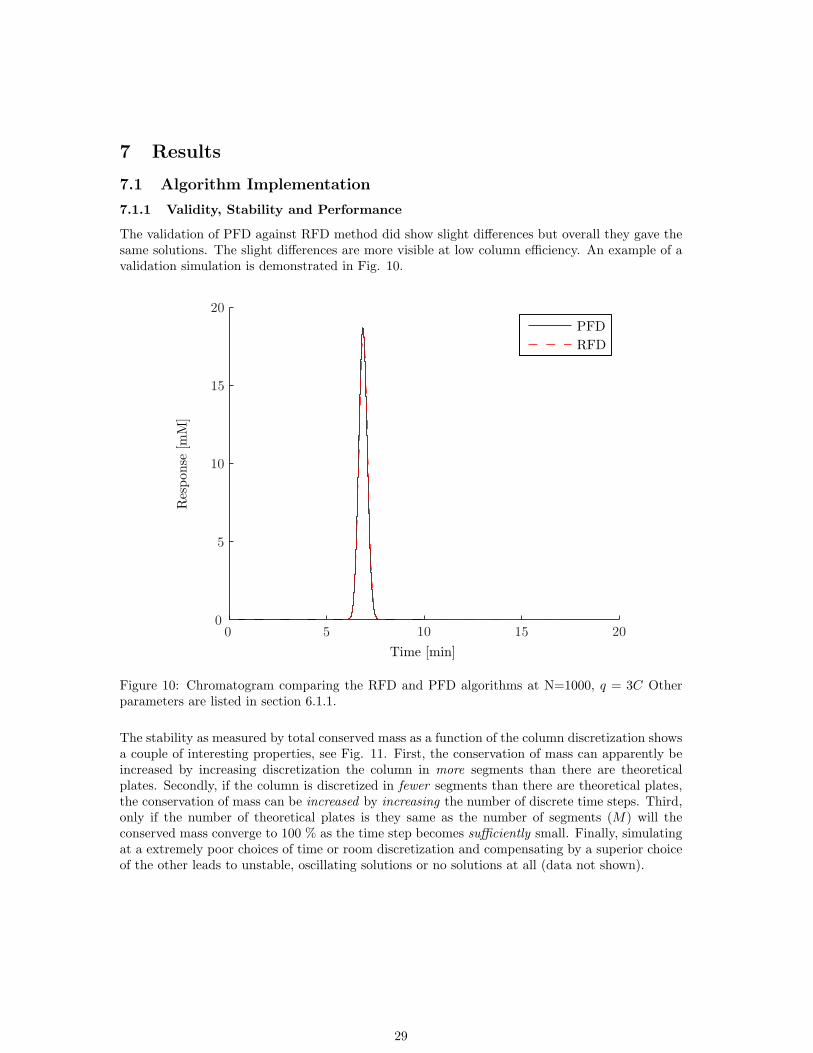
The validation of PFD against RFD method did show slight differences but overall they gave thesame solutions. The slight differences are more visible at low column efficiency. An example of avalidation simulation is demonstrated in Fig. 10.

Time [min]

Res

pons

e[m

M]

PFDRFD

0 5 10 15 200

5

10

15

20

Figure 10: Chromatogram comparing the RFD and PFD algorithms at N=1000, q = 3C Otherparameters are listed in section 6.1.1.

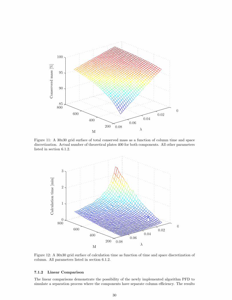
The stability as measured by total conserved mass as a function of the column discretization showsa couple of interesting properties, see Fig. 11. First, the conservation of mass can apparently beincreased by increasing discretization the column in more segments than there are theoreticalplates. Secondly, if the column is discretized in fewer segments than there are theoretical plates,the conservation of mass can be increased by increasing the number of discrete time steps. Third,only if the number of theoretical plates is they same as the number of segments (M) will theconserved mass converge to 100 % as the time step becomes sufficiently small. Finally, simulatingat a extremely poor choices of time or room discretization and compensating by a superior choiceof the other leads to unstable, oscillating solutions or no solutions at all (data not shown).

29

M λ

Con

serv

erd

mas

s[%

]

200

400

600

8000

0.020.04

0.060.08

85

90

95

100

Figure 11: A 30x30 grid surface of total conserved mass as a function of column time and spacediscretization. Actual number of theoretical plates 400 for both components. All other parameterslisted in section 6.1.2.

M λ

Cal

cula

tion

tim

e[m

in]

200

400

600

8000

0.020.04

0.060.08

0

1

2

3

Figure 12: A 30x30 grid surface of calculation time as function of time and space discretization ofcolumn. All parameters listed in section 6.1.2.

7.1.2 Linear Comparison

The linear comparisons demonstrate the possibility of the newly implemented algorithm PFD tosimulate a separation process where the components have separate column efficiency. The results

30

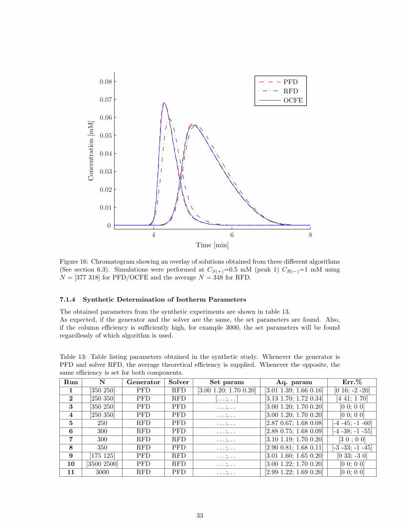
from one comparison is listed in Table 12. and in Figure 13. Neither algorithm exactly returnsthe set column efficiency but PFD performs better than RFD.

Table 12: Results from the comparison of RFD and PFD algorithms at linear conditions. Theefficiency was measured using equation 2.2. The discrepancy is measured as the relative differencebetween measured and set theoretical column efficiency. Actual error made by RFD is thereforelarger than stated.

Set N Measured N Discrepancy[%]P1 P2 P1 P2 P1 P2

PFD Nreal 3393 2862 3508 2886 4 0PFD Navg 3128 3128 3238 3167 4 1RFD Navg 3128 3128 2624 2886] 16 8

PFD Nreal

PFD Navg

RFD Navg

Time [min]

Res

pons

e[m

M]

0 2 4 6 8 100

0.5

1

1.5

2

Figure 13: A simulated chromatogram at non-overloaded linear conditions demonstrating theeffects of using the actual or the average theoretical efficiency of methyl mandelate (See Section6.1.2)

31

7.1.3 Nonlinear Comparisons

The comparison between the solutions obtained with RFD, PFD and OCFE shows a numberof trends. First, the solutions of PFD and OCFE are almost identical, no matter the choice oftheoretical efficiency or sample concentrations or different ratios between sample concentrations.At high column efficiency, at least for N ≥ 1500 there is practically no difference in the solutions(See figure 14). However, at lower efficiency, the solutions obtained with RFD diverges from thatof PFD/OCFE. In this study, it’s clearly noticeable for N ≤ 1000 (See figure 15). Decreasing theefficiency even further, RFD diverges even further (See figure 16).

Time [min]

Con

cent

ration

[mM

]

PFDRFDOCFEEXP

4 6 80

0.02

0.04

0.06

0.08

Figure 14: Chromatogram showing an overlay of solutions obtained from three different algorithmsand experimental data from the methyl mandelate separation on the AGP column (See section6.3). Simulations were performed at CS(+)=0.5 mM (peak 1) CR(−)=1 mM using measuredN = [3393 2862] for PFD/OCFE and the average N = 3128 for RFD.

PFDRFDOCFE

Time [min]

Con

cent

ration

[mM

]

4 6 80

0.02

0.04

0.06

0.08

Figure 15: Chromatogram showing an overlay of solutions obtained from three different algorithms(See section 6.3). Simulations were performed at CS(+)=0.5 mM (peak 1) CR(−)=1 mM usingN = [754 636] for PFD/OCFE and the average N = 695 for RFD.

32

PFDRFDOCFE

Time [min]

Con

cent

ration

[mM

]

4 6 80

0.01

0.02

0.03

0.04

0.05

0.06

0.07

0.08

Figure 16: Chromatogram showing an overlay of solutions obtained from three different algorithms(See section 6.3). Simulations were performed at CS(+)=0.5 mM (peak 1) CR(−)=1 mM usingN = [377 318] for PFD/OCFE and the average N = 348 for RFD.

7.1.4 Synthetic Determination of Isotherm Parameters

The obtained parameters from the synthetic experiments are shown in table 13.As expected, if the generator and the solver are the same, the set parameters are found. Also,if the column efficiency is sufficiently high, for example 3000, the set parameters will be foundregardlessly of which algorithm is used.

Table 13: Table listing parameters obtained in the synthetic study. Whenever the generator isPFD and solver RFD, the average theoretical efficiency is supplied. Whenever the opposite, thesame efficiency is set for both components.

Run N Generator Solver Set param Aq. param Err.%1 [350 250] PFD RFD [3.00 1.20; 1.70 0.20] [3.01 1.39; 1.66 0.16] [0 16; -2 -20]2 [250 350] PFD RFD [. . . ;. . . ] [3.13 1.70; 1.72 0.34] [4 41; 1 70]3 [350 250] PFD PFD . . . ;. . . [3.00 1.20; 1.70 0.20] [0 0; 0 0]4 [250 350] PFD PFD . . . ;. . . [3.00 1.20; 1.70 0.20] [0 0; 0 0]5 250 RFD PFD . . . ;. . . [2.87 0.67; 1.68 0.08] [-4 -45; -1 -60]6 300 RFD PFD . . . ;. . . [2.88 0.75; 1.68 0.09] [-4 -38; -1 -55]7 300 RFD RFD . . . ;. . . [3.10 1.19; 1.70 0.20] [3 0 ; 0 0]8 350 RFD PFD . . . ;. . . [2.90 0.81; 1.68 0.11] [-3 -33; -1 -45]9 [175 125] PFD RFD . . . ;. . . [3.01 1.60; 1.65 0.20] [0 33; -3 0]10 [3500 2500] PFD RFD . . . ;. . . [3.00 1.22; 1.70 0.20] [0 0; 0 0]11 3000 RFD PFD . . . ;. . . [2.99 1.22; 1.69 0.20] [0 0; 0 0]

33

7.2 Methyl Mandelate on AGP Column

The following data was obtained from linear and non-linear injections of methyl mandelate anddetermination of isotherm parameters.

Table 14: Parameters obtained from methyl mandelate separation on AGP columnAdsorption isotherm Bi-LangmuirParameters 1 [a1 b1 a2 b2] [3.065 146.61 4.859 3595]Parameters 2 [a1 b1 a2 b2] [3.281 318.33 7.020 4489]Theoretical plates [3393 2862]Flow [ml/min], t0 [min] 0.7,1.3

Excellent fitting of parameters to experimental chromatograms was obtained, See fig. 14. Furtherexemplifying injections are shown in figures 17 and 18.

a

Time [min]

Con

cent

ration

[mM

]

b

Time [min]

Con

cent

ration

[mM

]

c

Time [min]

Con

cent

ration

[mM

]

d

Time [min]

Con

cent

ration

[mM

]

0 2 4 6 80 2 4 6 8

0 2 4 6 80 2 4 6 8

0

0.05

0.1

0

0.05

0.1

0

0.05

0.1

0

0.05

0.1

Figure 17: Chromatograms of four racemic injections of methyl mandelate on the AGP column.a) CS(+)=0.5 mM (peak 1) CR(−)=1 mM b) CS(+)=0.25 mM CR(−)=1 mM c) CS(+)=1 mMCR(−)=0.5 mM d) CS(+)=1 mM CR(−)=0.25 mM

34

PSfrag

a

Time [min]

Con

cent

ration

[mM

]

1mM0.5mM0.25mM0.125mM

b

Time [min]

Con

cent

ration

[mM

]

1mM0.5mM0.25mM0.125mM

0 2 4 6 8

0 2 4 6 8

0

0.02

0.04

0.06

0.08

0

0.05

0.1

Figure 18: Overlayed chromatograms of single component injections of different injections concen-trations of methyl mandelate on AGP column.

7.3 Methyl Mandelate on Chiral Cellulose Column

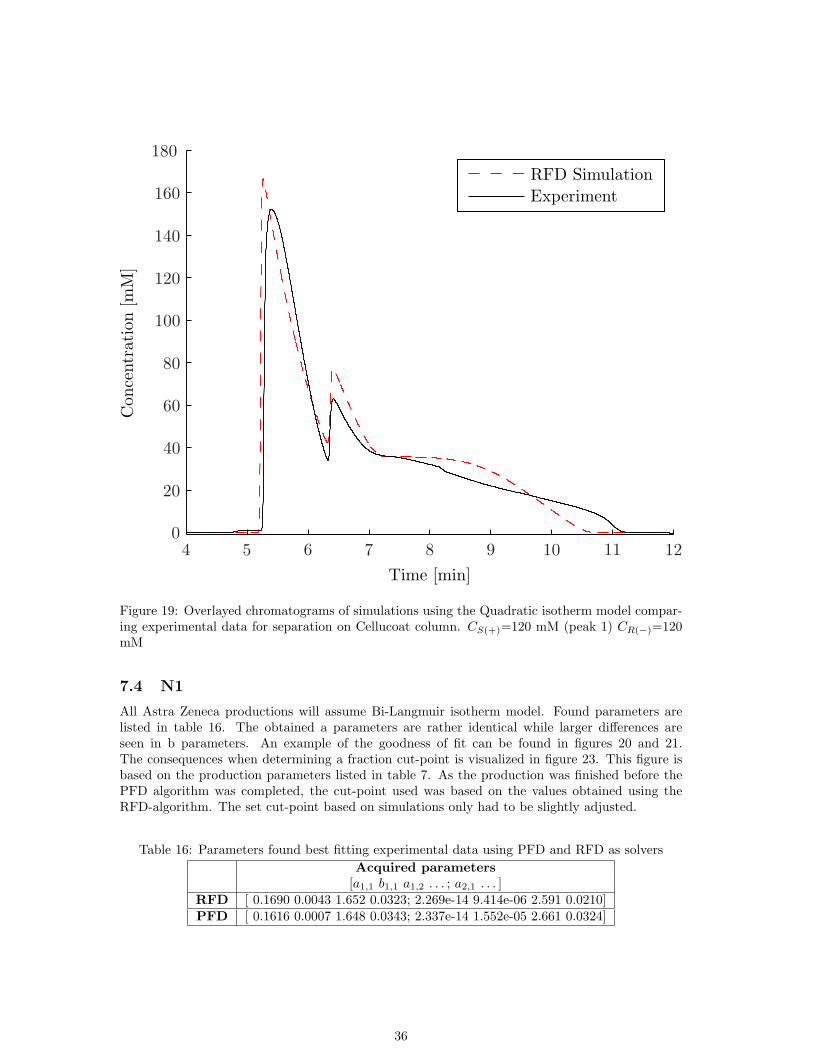
The search for parameters of the quadratic isotherm model fitting experimental chromatogramsfound parameters listed in table 15. The parameters found doesn’t fit experimental data very well(See fig 19).

Table 15: Parameters obtained from methyl mandelate separation on Kromasil Cellucoat columnAdsorption isotherm QuadraticParameters 1 [0.6116 1.886 0.1305 1.960 0.2351 5.408 0.0225 1.113]Parameters 2 [0.0004 3.003 2.943 0.0255 1.350 3.543 0.0393 0.0049]Theoretical plates [6247 5520]Flow [ml/min], t0 [min] 1,2.8

35

Con

cent

ration

[mM

]

Time [min]

RFD SimulationExperiment

4 5 6 7 8 9 10 11 120

20

40

60

80

100

120

140

160

180

Figure 19: Overlayed chromatograms of simulations using the Quadratic isotherm model compar-ing experimental data for separation on Cellucoat column. CS(+)=120 mM (peak 1) CR(−)=120mM

7.4 N1

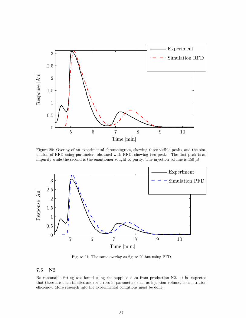
All Astra Zeneca productions will assume Bi-Langmuir isotherm model. Found parameters arelisted in table 16. The obtained a parameters are rather identical while larger differences areseen in b parameters. An example of the goodness of fit can be found in figures 20 and 21.The consequences when determining a fraction cut-point is visualized in figure 23. This figure isbased on the production parameters listed in table 7. As the production was finished before thePFD algorithm was completed, the cut-point used was based on the values obtained using theRFD-algorithm. The set cut-point based on simulations only had to be slightly adjusted.

Table 16: Parameters found best fitting experimental data using PFD and RFD as solversAcquired parameters

[a1,1 b1,1 a1,2 . . . ; a2,1 . . . ]RFD [ 0.1690 0.0043 1.652 0.0323; 2.269e-14 9.414e-06 2.591 0.0210]PFD [ 0.1616 0.0007 1.648 0.0343; 2.337e-14 1.552e-05 2.661 0.0324]

36

Time [min]

Res

pons

e[A

u]

Experiment

Simulation RFD

5 6 7 8 9 100

0.5

1

1.5

2

2.5

3

Figure 20: Overlay of an experimental chromatogram, showing three visible peaks, and the sim-ulation of RFD using parameters obtained with RFD, showing two peaks. The first peak is animpurity while the second is the enantiomer sought to purify. The injection volume is 150 µl

Time [min.]

Res

pons

e[A

u]

Experiment

Simulation PFD

5 6 7 8 9 100

0.5

1

1.5

2

2.5

3

Figure 21: The same overlay as figure 20 but using PFD

7.5 N2

No reasonable fitting was found using the supplied data from production N2. It is suspectedthat there are uncertainties and/or errors in parameters such as injection volume, concentrationefficiency. More research into the experimental conditions must be done.

37

Product RFDWaste RFDProduct PFDWaste PFD

Time [min]

Con

cent

ration

[g/l

]

3.5 4 4.5 5 5.5 6 6.5 7

1

2

3

4

5

6

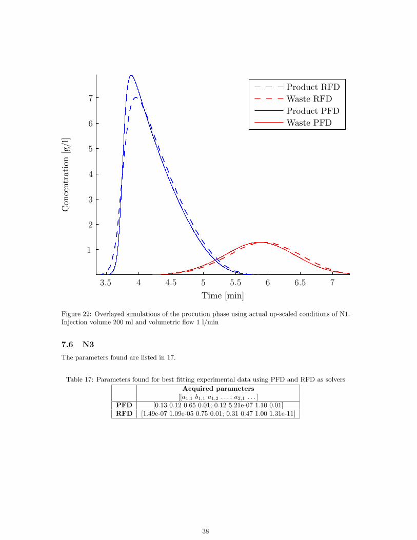
7

Figure 22: Overlayed simulations of the procution phase using actual up-scaled conditions of N1.Injection volume 200 ml and volumetric flow 1 l/min

7.6 N3

The parameters found are listed in 17.

Table 17: Parameters found for best fitting experimental data using PFD and RFD as solversAcquired parameters

[[a1,1 b1,1 a1,2 . . . ; a2,1 . . . ]PFD [0.13 0.12 0.65 0.01; 0.12 5.21e-07 1.10 0.01]RFD [1.49e-07 1.09e-05 0.75 0.01; 0.31 0.47 1.00 1.31e-11]

38

tcut [min]

%

Purity RFDYield RFDPurity PFDYield PFD

4.7 4.8 4.9 5 5.1 5.2 5.3 5.4 5.586

88

90

92

94

96

98

100

Figure 23: The purity and yield graph of the scaled up N1 production (See Fig. 22 comparingparameters obtained using RFD and PFD. The cut-point used in the actual production was onlyslightly adjusted from the one obtained with simulations using RFD. PFD was not yet implemetedat the time of production.

39

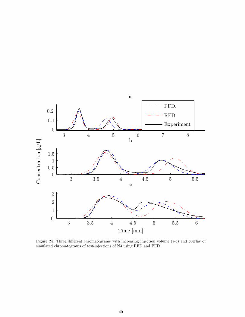
a

PFD.

RFD

Experiment

b

Con

cent

ration

[g/L

]

c

Time [min]3 3.5 4 4.5 5 5.5 6

3 3.5 4 4.5 5 5.5

3 4 5 6 7 8

0

1

2

3

00.5

11.5

0

0.1

0.2

Figure 24: Three different chromatograms with increasing injection volume (a-c) and overlay ofsimulated chromatograms of test-injections of N3 using RFD and PFD.

40

8 Conclusions and Discussion

What conclusions can be drawn about the solutions to eq. 4.5 obtained by the PFD-algorithm?All comparisons with OCFE points to that PFD always converge to the true solution, regardlessof the conditions of the simulation. As has been suspected, RFD seems to diverge from this truesolution at low column efficiency. It is unclear from the technical perspective why this happens.The choices of dt and dx in the RFD algorithm should assure both stability and accurate approx-imation of physical dispersion but apparently don’t.

It is still uncertain how solutions compare when simulating more than two components, neitherhow large differences in column efficiencies between components affect the solution.

It also remains to investigate the concept of stability. In this work, stability has been equaled toconservation of mass. It is reasonable to equate loss of mass to algorithm instability but if theopposite really is true is more uncertain. Nevertheless, in the comparsions with OCFE, dt wasdynamically adjusted to reach at least 97% conservation of mass and this apparently works well.As I understand, it is impossible to ensure global stability when solving a PDE of this kind. Itshould however be possible to derive stability criteria for linear isotherms and use this criteria asguidelines when simulating non-linear isotherms.

What also have been shown is superiority of the RFD when it comes to calculation time. Therehas been no evidence of the need to use PFD at high column efficiency, where solutions appearidentical. Here, RFD will find solutions many orders of magnitude faster than PFD.

Regarding the Astra Zeneca productions, I feel reluctant to draw any certain conclusions. Pro-duction N1 finds similar parameters, as does N3. Overlays of the experiments and simulationsshow markedly differences but they are still unquantified. All work with Astra Zeneca data hasbeen rather troublesome, partly because there exists contaminants. It is impossible to quantify ifor how much they interfere with the adsorption process of the components one actually models.Then, there are uncertainties in the measured column efficiencies, lack of experimental injectionprofiles etc. This is however the reality at Astra Zeneca, there isn’t the time to perform the samethorough experiments as for example were performed in this project (for example methyl mande-late on AGP column).

Despite the uncertainties, a successfull simulation of a production process for production N1 wasmade, enabeling us to estimate a fraction cut-point wich only had to be slightly adjusted in theactual process.

I think Astra Zeneca should perform a more thorough investigation at least once. By doing so,one could really evaluate the applicability of modeling and numerical modeling. One should thentry to identify exactly which of the uncertainties I have seen in N1-N3 which most affects the solu-tion. If these can be found, RFD/PFD could become a valuable tool. If not, it is still a usable tool.

Finally, PFD should be implemented in the inverse solver and be invoked whenever simulatingunder 1000 theoretical plates. However, RFD should first do the coarse work of finding acceptableparameters. If calculation time is of less importance, or could be significantly optimized for speed,there would be no need to use RFD at all, since, ultimatley it diverges from the true solution of 4.5.

What about the failed attempts to fit a model to the methyl mandelate separation on a chiralcellulose column? Many weeks of work with this experiment has revealed a peculiar adsorptionbehaviour. A suitable model has not been found and neither an explaination of the mechanismbehind the observed behaviour. More investigations are needed. Atleast theoretically it should bepossible to fit the Quadratic isotherm.

41

9 Acknowledgements

I wish to thank Dr. Robert Arnell and Catrine Fredlund at Astra Zeneca for giving me the op-portunity to do my degree project there. Prof. Torgny Fornstedt for arranging this interestingcollaboration between the university and Astra Zeneca and for always keeping my spirit high.

Dr. Jorgen Samuelsson for invaluable help both with the implementation of the algorithm, exper-imental set-up and many discussions at work, at coffee breaks, at lunch, about chromatography.Patrik Forssen at SweCrown AB for technical advice about programming MATLAB and Fortranand for continuously questioning the details of my implementations.

Prof. Per Lotstedt at the Division of Scientific Computing for discussion about numerical stabilityof the algorithm. Albeit inconclusive, these discussions made me more at ease.

Simon, Staffan and Kerstin at Astra Zeneca PR&D Large Scale Chromatography Team, you’vetaught me a bit about the reality of working large-scale chromatography.

I would also like to thank Prof. Krzysztof Kaczmarski at Rzeszow University of Technology forengaging in my synthetic algorithm comparison study. Thanks to your incredible fast and thor-ough work, I could make the crucial comparison between PFD and OCFE.

A final thanks go to group members Torgny Undin and Lena Edstrom and all other personnel atthe Department of Physical and Analytical Chemistry and Astra Zeneca Sodertalje, you’ve mademy stay both pleasant and rewarding.

42

References

E. Anderson, Z. Bai, C. Bischof, S. Blackford, J. Demmel, J. Dongarra, J. Du Croz, A. Green-baum, S. Hammarling, A. McKenney, and D. Sorensen. LAPACK Users’ Guide. Society forIndustrial and Applied Mathematics, Philadelphia, PA, third edition, 1999. ISBN 0-89871-447-8(paperback).

R. Arnell. Development and validation of methods for characterization of multi-component systemsin preparative LC. Acta Universitatis Upsaliensis, 2006.

Jack Cazes and Raymand P. W. Scott. Chromatography Theory. Marcel Dekker, 2002.

Geoffrey B. Cox. Preparative Enantioselective Chromatography. Blackwell Publishing, 2005.

A. Felinger, A. Cavazzini, and G. Guiochon. Numerical determination of the competitive isothermof enantiomers. Journal of Chromatography A, 986(2):207–225, 2003.

T. Fornstedt, G. Gotmar, M. Andersson, and G. Guiochon. Dependence on the mobile-phase pHof the adsorption behavior of propranolol enantiomers on a cellulase protein used as the chiralselector. J. Am. Chem. Soc, 121(6):1164–1174, 1999.

P. Forssen. Adsorption Isotherm Parameter Estimation in Nonlinear Liquid Chromatography.Uppsala universitet, Fakultetsovergripande enheter, Acta Universitatis Upsaliensis, 2005.

P. Forssen, R. Arnell, and T. Fornstedt. An improved algorithm for solving inverse problems inliquid chromatography. Computers and Chemical Engineering, 30(9):1381–1391, 2006.

G. Guiochon. Preparative liquid chromatography. Journal of Chromatography A, 965(1-2):129–161, 2002.

Georges Guiochon and Bingchang Lin. Modeling for Preparative Chromatography. Academic Press,Elsevier, 2003.

Georges Guiochon, Attila Felinger, Dean G. Shirazi, and Anita M. Katti. Fundamentals of Prepar-ative and Nonlinear Chromatography 2nd Ed. Elsevier Academic Press, 2006.

Daniel C. Harris. Quantitative Chemical Analysis 6th ed. W.H. Freemand And Company, 2003.

K. Kaczmarski. Estimation of adsorption isotherm parameters with inverse method—Possibleproblems. Journal of Chromatography A, 1176(1-2):57–68, 2007.

P. Rouchon, M. Schonauer, P. Valentin, and G. Guiochon. Numerical simulation of band propaga-tion in nonlinear chromatography. Separation Science and Technology, 22(8):1793–1833, 1987.

J. Samuelsson. Development of methods for phase system characterization in liquid chromatogra-phy. Acta Universitatis Upsaliensis, 2008.

Henner Schmidt-Traub. Preparative Chromatography. Wiley-VCH, 2005.

Y. Zhang, S. Rohani, and A.K. Ray. Numerical determination of competitive adsorption isothermof mandelic acid enantiomers on cellulose-based chiral stationary phase. Journal of Chromatog-raphy A, 1202(1):34–39, 2008.

43