Vehicle System Dynamics An improved Magic Formula…mate.tue.nl/mate/pdfs/12478.pdf · Since its...

PLEASE SCROLL DOWN FOR ARTICLE

This article was downloaded by: [Technische Universiteit - Eindhoven]On: 29 November 2010Access details: Access Details: [subscription number 919362742]Publisher Taylor & FrancisInforma Ltd Registered in England and Wales Registered Number: 1072954 Registered office: Mortimer House, 37-41 Mortimer Street, London W1T 3JH, UK

Vehicle System DynamicsPublication details, including instructions for authors and subscription information:http://www.informaworld.com/smpp/title~content=t713659010

An improved Magic Formula/Swift tyre model that can handle inflationpressure changesI. J. M. Besselinka; A. J. C. Schmeitzb; H. B. Pacejkac

a Department of Mechanical Engineering, Eindhoven University of Technology, Eindhoven, TheNetherlands b TNO Automotive, Helmond, The Netherlands c TU Delft, Delft, The Netherlands

Online publication date: 26 November 2010

To cite this Article Besselink, I. J. M. , Schmeitz, A. J. C. and Pacejka, H. B.(2010) 'An improved Magic Formula/Swift tyremodel that can handle inflation pressure changes', Vehicle System Dynamics, 48: 1, 337 — 352To link to this Article: DOI: 10.1080/00423111003748088URL: http://dx.doi.org/10.1080/00423111003748088

Full terms and conditions of use: http://www.informaworld.com/terms-and-conditions-of-access.pdf

This article may be used for research, teaching and private study purposes. Any substantial orsystematic reproduction, re-distribution, re-selling, loan or sub-licensing, systematic supply ordistribution in any form to anyone is expressly forbidden.

The publisher does not give any warranty express or implied or make any representation that the contentswill be complete or accurate or up to date. The accuracy of any instructions, formulae and drug dosesshould be independently verified with primary sources. The publisher shall not be liable for any loss,actions, claims, proceedings, demand or costs or damages whatsoever or howsoever caused arising directlyor indirectly in connection with or arising out of the use of this material.

http://www.informaworld.com/smpp/title~content=t713659010

http://dx.doi.org/10.1080/00423111003748088

http://www.informaworld.com/terms-and-conditions-of-access.pdf

Vehicle System DynamicsVol. 48, Supplement, 2010, 337–352

An improved Magic Formula/Swift tyre model thatcan handle inflation pressure changes

I.J.M. Besselinka*, A.J.C. Schmeitzb and H.B. Pacejkac

aDepartment of Mechanical Engineering, Eindhoven University of Technology, P.O. Box 513, 5600 MBEindhoven, The Netherlands; bTNO Automotive, Helmond, The Netherlands; cTU Delft, Delft,

The Netherlands

(Received 19 October 2009; final version received 3 March 2010 )

This paper describes extensions to the widely used TNO MF-Tyre 5.2 Magic Formula tyre model.The Magic Formula itself has been adapted to cope with large camber angles and inflation pressurechanges. In addition, the description of the rolling resistance has been improved. Modelling of the tyredynamics has been changed to allow a seamless and consistent switch from simple first-order relaxationbehaviour to rigid ring dynamics. Finally, the effect of inflation pressure on the loaded radius and thetyre enveloping properties is discussed and some results are given to illustrate the capabilities of themodel.

Keywords: simulation; tyre dynamics models; tyre dynamics measurement; tyre dynamics; MagicFormula

1. Introduction

Since its conception over 20 years ago, the Magic Formula has fairly quickly been adoptedas the industry standard tyre model for vehicle handling simulations. Over the years variousdevelopments have been made to improve the accuracy and to extend the capabilities ofthe model, for example, the method to describe combined slip has been improved and aspecial Magic Formula has been developed to handle the large camber angles occurring onmotorcycles. In parallel, research has been done to increase the frequency range by introducingrigid ring dynamics, contact patch transients and an obstacle enveloping model, also knownas the SWIFT or MF-Swift model. An overview and description of these developments canbe found in Pacejka [1].

The fact that from the start the tyre model equations were published in the open literaturehas certainly contributed to the popularity of the Magic Formula. On the other hand, over theyears it has also resulted in a number of different, at times incompatible, implementations.Different versions of the Magic Formula may be used, equations are sometimes partiallyimplemented, in-house extensions are added, different axis system or units are used, etc.

*Corresponding author. Email: [email protected]

ISSN 0042-3114 print/ISSN 1744-5159 online© 2010 Taylor & FrancisDOI: 10.1080/00423111003748088http://www.informaworld.com

Downloaded By: [Technische Universiteit - Eindhoven] At: 07:10 29 November 2010

338 I.J.M. Besselink et al.

Notwithstanding these issues, the TNO MF-Tyre 5.2 tyre model has reached a mature statusand is widely used in the industry for vehicle handling studies. The model equations aredocumented in TNO [2].

To move forward from MF-Tyre 5.2, several targets have been defined:

• To improve the description of camber, that is, to have an explicit formulation and controlover the camber stiffness and to extend the capabilities of the model for handling very largecamber angles. This will make the special ‘motorcycle’ Magic Formula superfluous andimproves processing of measurements according to the TIME procedure.

• To include the effect of inflation pressure changes in the Magic Formula. This will eliminatethe need to have separate parameter sets (tyre property files) for different tyre pressures. Itwill allow evaluating tyre behaviour for pressures not in the measurement programme andit also leads to a reduction in the total number of measurements required.

• To make the description of tyre dynamics consistent between MF-Swift and MF-Tyre. Forexample, when including the dynamics of the tyre belt, the path-dependent (basic) tyrerelaxation behaviour should remain unchanged.

In addition, various other enhancements have been made, for example, in the description ofrolling resistance and overturning moment. This paper aims to introduce the MF-Tyre/MF-Swift 6.1 model and accompanying equations. Due to space restrictions and the extent of thechanges that were made in comparison with the MF-Tyre 5.2 model, turn slip extensions [1]will not be discussed.

2. Contact point, loaded radius and calculation of slip

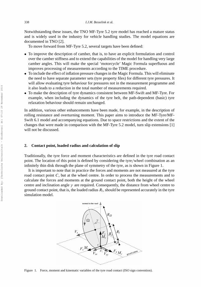
Traditionally, the tyre force and moment characteristics are defined in the tyre road contactpoint. The location of this point is defined by considering the tyre/wheel combination as aninfinitely thin disk through the plane of symmetry of the tyre, as is shown in Figure 1.

It is important to note that in practice the forces and moments are not measured at the tyreroad contact point C, but at the wheel centre. In order to process the measurements and tocalculate the forces and moments at the ground contact point, both the height of the wheelcentre and inclination angle γ are required. Consequently, the distance from wheel centre toground contact point, that is, the loaded radius Rl , should be represented accurately in the tyresimulation model.

Figure 1. Force, moment and kinematic variables of the tyre road contact (ISO sign convention).


Vehicle System Dynamics 339

First, centrifugal growth of the free tyre radius R� is calculated using the following formula:

R� = R0

(qre0 + qv1

(�R0

V0

)2)

, (1)

where R0 equals the non-rolling free tyre radius, V0 a reference velocity, � the wheel rotationalvelocity and qre0 and qv1 the model parameters. The tyre deflection ρ is the difference betweenthe free tyre radius R� and the loaded tyre radius Rl:

ρ = max(R� − Rl, 0). (2)

The vertical tyre force Fz is then calculated using the following formula:

Fz =(

1 + qv2R0

V0|�| −

(qFcxFx

Fz0

)2

−(

qFcyFy

Fz0

)2) (

qFz1ρ

R0+ qFz2

(ρ

R0

)2)

· (1 + pFz1 dpi )Fz0. (3)

Various effects are included in this calculation: a stiffness increase with velocity (qv2), ver-tical sinking due to longitudinal and lateral forces (qFcx, qFcy), a quadratic force deflectioncharacteristic (qFz1, qFz2) and the influence of the tyre inflation pressure (pFz1). Further, Fz0

is the nominal load and dpi the non-dimensional pressure increment, see appendix. For largecamber angles (e.g. motorcycle tyres), a modified approach for calculating the vertical forceis necessary, taking into account the contour of the tyre. Its discussion is outside the scope ofthis paper.

The vertical stiffness cz0 at the nominal vertical load, nominal inflation pressure, notangential forces and zero forward velocity can be calculated as follows:

cz0 = Fz0

R0

√q2

Fz1 + 4qFz2. (4)

In the expressions for the effective rolling radius and contact patch dimensions, the verticalstiffness adapted for tyre inflation pressure is used:

cz = cz0(1 + pFz1 dpi ). (5)

The forces (Fx , Fy) and moments (Mx , My , Mz) at the ground contact point are functions ofvertical force Fz, various slip properties, inclination angle γ , forward velocity Vx and inflationpressure pi . These nonlinear relations are captured in the Magic Formula. The longitudinalslip is defined as the ratio of the longitudinal slip velocity Vsx and forward velocity Vx :

κ = −Vsx

Vx

= −Vx − �Re

Vx

= −�fr − �

�fr= �

�fr− 1. (6)

In this equation, �fr is the angular velocity of the freely rolling tyre. When executing mea-surements the latter part of this equation may be used to determine the amount of longitudinalslip. In the tyre simulation model, the first part of the equation is used, requiring an explicitequation for the effective rolling radius Re. The ratio of the forward velocity of the wheelcentre Vx to the angular velocity of the free rolling tyre �fr equals the effective rolling radiusRe. The following empirical formula is used:

Re = R� − Fz0

cz

(Dreff arctan

(Breff

Fz

Fz0

)+ Freff

Fz

Fz0

), (7)

where Dreff , Breff and Freff are model parameters. When no measurements are available, thesuggested values are Dreff = 0.24, Breff = 8 and Freff = 0.01. The effective rolling radius



defines the slip point S. Note that the location of S is different from the contact point C as isshown in Figure 1. Point S is also used to calculate the sideslip angle α using the lateral slipvelocity Vsy:

α = arctan

(Vsy

Vx

). (8)

It is clear that in order to get an accurate representation of the tyre characteristics consis-tent definitions for slip should be used. Though one can argue on the exact definition of slipvariables, it is clear that in any case consistent definitions should be used for both the mea-surements and the simulation model. The definitions given in this section have been used since1996 in the various MF-Tyre simulation models (including MF-Tyre 5.2). When modellingthe tyre-road enveloping and relaxation behaviour the dimensions of the tyre contact patchare needed. The empirical expressions for half of the contact length a and half of the width b

read as follows:

a = R0

(qra2

Fz

czR0+ qra1

√Fz

czR0

)≈ R0

(qra2

ρ

R0+ qra1

√ρ

R0

), (9)

b = w

(qrb2

Fz

czR0+ qrb1

(Fz

czR0

)1/3)

≈ w

(qrb2

ρ

R0+ qrb1

(ρ

R0

)1/3)

, (10)

where w is the nominal width of the tyre. Since these expressions are functions of the tyredeflection ρ, the effect of changing the tyre inflation pressure is taken into account. Loweringthe inflation pressure results in an increase in tyre deflection and thus an increase in contactlength.

3. Steady-state force and moment characteristics

For an introduction to Magic Formula tyre modelling, we refer to Pacejka [1, pp. 172–184].Initially, the Magic Formula has been designed to describe the force and moment characteristicsof passenger car tyres within a limited camber range (±15◦). Beyond this range extrapolationerrors may occur and as such the formula proved not to be suitable for describing tyre char-acteristics at large inclination angles. This resulted in a different Magic Formula equation formotorcycle tyres, as proposed by De Vries [3], where the contributions of camber and sideslipare fully separated, as is shown in Equation (11):

Fy = Dy sin

(Cy arctan((1 − Ey)Byαy + Ey arctan(Byαy))

+ Cγ arctan((1 − Eγ )Bγ γ + Eγ arctan(Bγ γ ))

). (11)

This approach was subsequently adopted in a slightly modified form for the MF–MC Tyremodel, aimed specifically at motorcycle tyres. This model is described in Pacejka [1, pp. 579–583]. One of the benefits of this approach is that the camber stiffness is defined explicitly,which also proves to be convenient when new approaches to tyre measurements, like theTIME procedure [4], are used. A logical step would be to also use the MF-MC Tyre modelfor passenger car tyres, but the accuracy proved to be less compared with the normal MagicFormula. An attempt was made to adapt the MF–MC Tyre model to suit passenger car tyrecharacteristics better, but this model, also known as MF-Time [5], still suffers from a reducedaccuracy with respect to the normal Magic Formula for passenger car tyres.



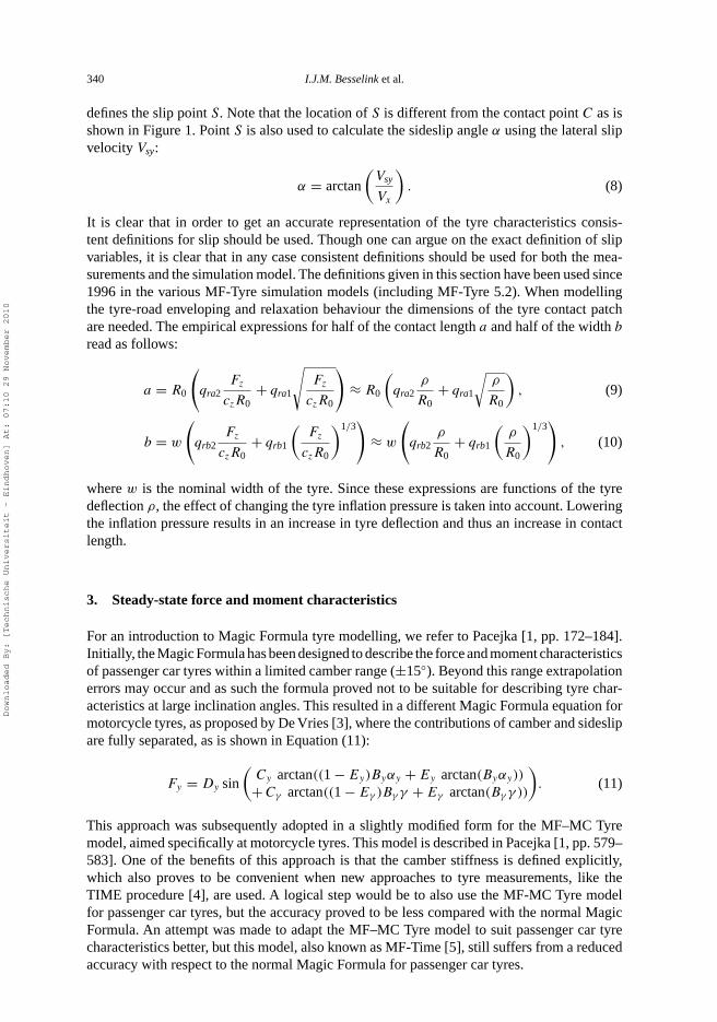
Figure 2. Creating the side force characteristic at an inclination angle by applying vertical and horizontal shifts.

It turns out that only limited modifications to the MF-Tyre 5.2 equations are required toovercome these issues. First, the vertical shift in the lateral force SVyγ due to camber (andvertical force) remains the same:

SVyγ = Fz(pVy3 + pVy4 dfz)γ, (12)

where dfz is the dimensionless load increment and pVy3 and pVy4 are some model parameters,see appendix. The camber stiffness Kyγ is specified in exactly the same way as in the MF–MCTyre model:

Kyγ = (pKy6 + pKy7 dfz)Fz. (13)

Now the required horizontal shift (or sideslip angle) due to camber can be calculated usingthe cornering stiffness Kyα:

SHyγ = Kyγ γ − SVyγ

Kyα

. (14)

This approach is illustrated in Figure 2. The side force characteristic is shifted vertically by amagnitude SVyγ to account for the increase in side force due to an inclination angle for largevalues of side slip. At zero side slip angle, we demand that the side force due to an inclinationof the tyre equals Kyγ γ . Since the slope of Fy versus α curve is known, it is equal to thecornering stiffness Kyα , the magnitude of the required horizontal shift can be easily calculatedusing Equation (14). In this simplified explanation, we ignore initial offsets for zero inclinationangle and changes of the shape of Fy versus α curve due to an inclination angle.

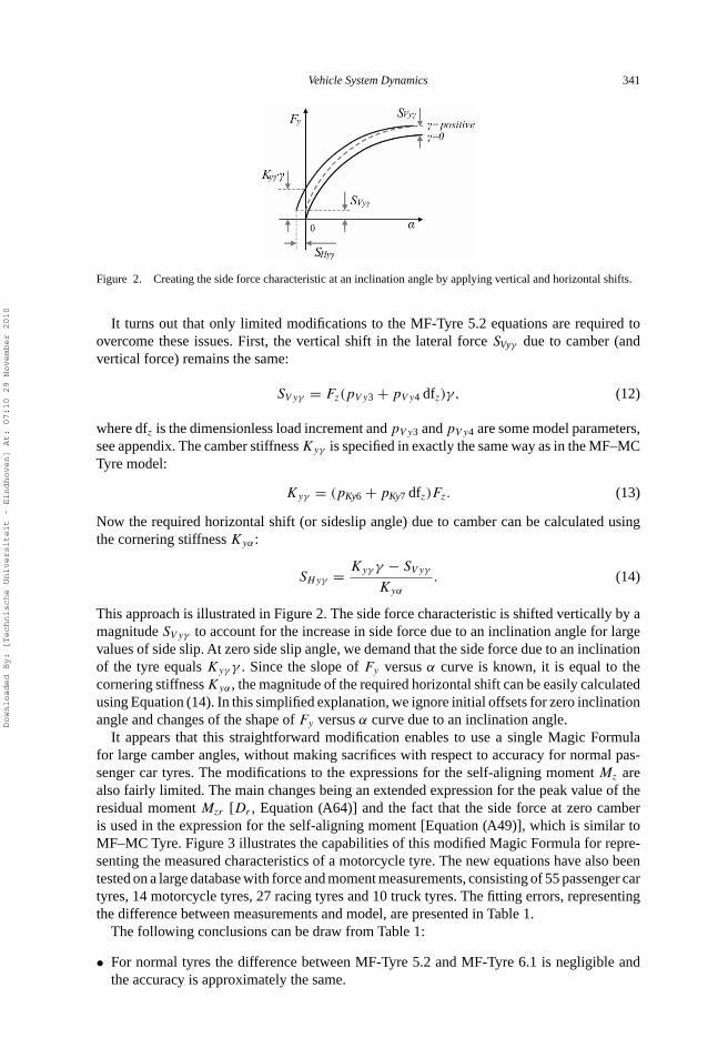
It appears that this straightforward modification enables to use a single Magic Formulafor large camber angles, without making sacrifices with respect to accuracy for normal pas-senger car tyres. The modifications to the expressions for the self-aligning moment Mz arealso fairly limited. The main changes being an extended expression for the peak value of theresidual moment Mzr [Dr , Equation (A64)] and the fact that the side force at zero camberis used in the expression for the self-aligning moment [Equation (A49)], which is similar toMF–MC Tyre. Figure 3 illustrates the capabilities of this modified Magic Formula for repre-senting the measured characteristics of a motorcycle tyre. The new equations have also beentested on a large database with force and moment measurements, consisting of 55 passenger cartyres, 14 motorcycle tyres, 27 racing tyres and 10 truck tyres. The fitting errors, representingthe difference between measurements and model, are presented in Table 1.

The following conclusions can be draw from Table 1:

• For normal tyres the difference between MF-Tyre 5.2 and MF-Tyre 6.1 is negligible andthe accuracy is approximately the same.



• The MF-Time model is less accurate in comparison with the MF-Tyre 5.2, in particular therepresentation of the self-aligning moment appears to be worse.

• MF-Tyre 6.1 can represent motorcycle tyre behaviour quite accurately: the fitting error ofthe side force characteristic is even reduced in comparison with the MF–MC Tyre, thoughthe self-aligning moment is somewhat less accurate.

So a single set of Magic Formula equations has been developed which can represent passengercar, truck, racing and motorcycle tyres with a similar accuracy as obtained with different magicformula tyre models used by the industry today. The MF-Tyre 6.1 equations have the advantageof including an explicit formulation of the camber stiffness and they can cope with large camberangles. Next, the expressions have been extended to include the effect of tyre inflation pressurechanges on the tyre force and moment characteristics.

It is clear that for many passenger cars on the road the same tyres are used on the front andrear axle, but the tyre pressure is different and may need to be adjusted for different vehicleloading conditions. The Magic Formula equations published to date do not account for tyrepressure changes, leading to multiple parameter datasets for different tyre pressures and anadditional measurement effort. Furthermore, only the inflation pressures tested can be selectedand it is not possible to perform an interpolation.

As the Magic Formula is a semi-empirical tyre model, each individual tyre characteristic hasto be analysed for the impact of changes to the tyre inflation pressure [6,7]. Both measurements

−5 0 5

−2000

−1000

0

1000

2000

α [deg.]

Fy [

N]

γ = −5°γ = 0°γ = 5°γ = 20°γ = 30°γ = 45°

−5 0 5−40

−30

−20

−10

0

10

20

30

α [deg.]

Mz [

Nm

]

Fz = 1475 N

Figure 3. MF-Tyre 6.1 fit of a motorcycle tyre, left: side force, right: self-aligning moment; markers aremeasurements (source: TNO Tyre Test Trailer) and continuous lines are Magic Formula results.

Table 1. Comparison of average fitting errors for various tyre models and different tyre types.

Car/truck/race tyres (n = 92) Motorcycle tyres (n = 14)

Force/slip case MF-Tyre 5.2 MF-Time MF-Tyre 6.1 MF−MC Tyre 1.1 MF-Tyre 6.1

Fx pure (%) 4.17 4.16 4.17 4.11 4.06Fy pure (%) 2.37 2.73 2.26 4.55 4.28Mz pure (%) 6.47 9.53 6.23 8.76 10.19Fx combined (%) 5.70 5.69 5.70 4.46 4.43Fy combined (%) 8.58 8.81 8.53 11.06 11.01Mz combined (%) 32.74 34.57 32.49 40.59 40.29



0 5000 100000

500

1000

1500

2000

Fz [N]

Cor

neri

ng s

tiffn

ess

[N/d

eg]

Measurements:

−5 0 5−300

−200

−100

0

100

200

300

α [deg]

Mz [

Nm

]

pi = p

i0− 0.6 bar

pi = p

i0

pi = p

i0 + 0.6 bar

Magic Formula

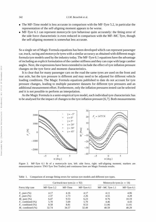
Figure 4. Tyre pressure effects for a passenger car tyre; left: cornering stiffness and right: self-aligning moment.

and a physical background model were used in this process. The main effects identified areas follows:

• changes in longitudinal slip stiffness, cornering stiffness and camber stiffness;• changes in peak friction coefficient, both longitudinal and lateral;• a reduction of the pneumatic trail with increasing inflation pressure.

Details on the modified equations can be found in the appendix. As an example, the corneringstiffness and self-aligning moment characteristics are shown in Figure 4. Since the effectof tyre inflation pressure on, for example, the combined slip characteristics is small, it issufficient to measure this behaviour at a single inflation pressure and the total number of testscan therefore be reduced. Details on the testing requirements can be found in the TNO tyremodel documentation [8].

As energy efficiency of road vehicles is becoming even more important, an accurate mod-elling of the rolling resistance of the tyres should be addressed. In the SWIFT model theincrease in rolling resistance at high forward velocities has already been identified. Next, thenonlinear dependency on the vertical force and inflation pressure has been added.

In Michelin [9], the following equation is given to adapt the rolling resistance for conditionsdeviating from the ISO rolling resistance test:

frr = frr,ISO

(pi

pi,ISO

)α (Fz

Fz,ISO

)β

, (15)

where frr is the rolling resistance coefficient, pi the tyre inflation pressure and Fz the verticaltyre force. According to Michelin [9], the following coefficients are applicable: α = −0.4 andβ = 0.85 for a passenger car and α = −0.2 and β = 0.9 for a truck tyre. This equation hasbeen adopted in a slightly modified form and has been combined with the existing velocityinfluence and reads (not including the camber effects) for the rolling resistance moment asfollows:

My = −R0Fz0λMy

(qsy1 + qsy2

Fx

Fz0+ qsy3

∣∣∣∣Vx

V0

∣∣∣∣ + qsy4

(Vx

V0

)4) (

Fz

Fz0

)qsy7(

pi

pi0

)qsy8

.

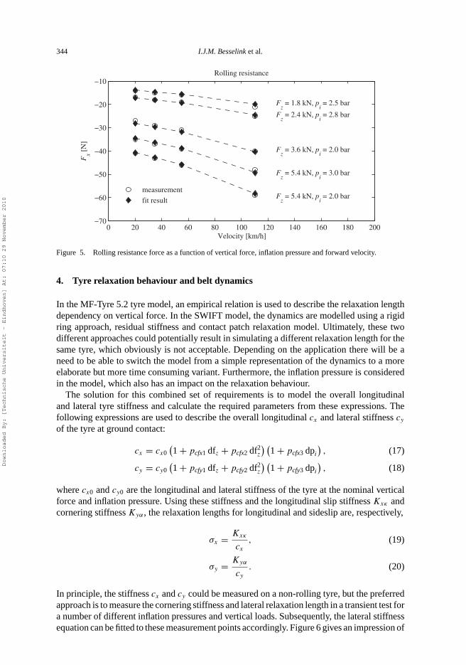
(16)Figure 5 shows that following this approach the rolling resistance can be modelled accuratelyfor a standard passenger car tyre.



0 20 40 60 80 100 120 140 160 180 200−70

−60

−50

−40

−30

−20

−10

Velocity [km/h]

Fx [

N]

Rolling resistance

Fz = 5.4 kN, p

i = 2.0 bar

Fz = 5.4 kN, p

i = 3.0 bar

Fz = 3.6 kN, p

i = 2.0 bar

Fz = 2.4 kN, p

i = 2.8 bar

Fz = 1.8 kN, p

i = 2.5 bar

measurement

fit result

Figure 5. Rolling resistance force as a function of vertical force, inflation pressure and forward velocity.

4. Tyre relaxation behaviour and belt dynamics

In the MF-Tyre 5.2 tyre model, an empirical relation is used to describe the relaxation lengthdependency on vertical force. In the SWIFT model, the dynamics are modelled using a rigidring approach, residual stiffness and contact patch relaxation model. Ultimately, these twodifferent approaches could potentially result in simulating a different relaxation length for thesame tyre, which obviously is not acceptable. Depending on the application there will be aneed to be able to switch the model from a simple representation of the dynamics to a moreelaborate but more time consuming variant. Furthermore, the inflation pressure is consideredin the model, which also has an impact on the relaxation behaviour.

The solution for this combined set of requirements is to model the overall longitudinaland lateral tyre stiffness and calculate the required parameters from these expressions. Thefollowing expressions are used to describe the overall longitudinal cx and lateral stiffness cy

of the tyre at ground contact:

cx = cx0(1 + pcfx1 dfz + pcfx2 df2

z

) (1 + pcfx3 dpi

), (17)

cy = cy0(1 + pcfy1 dfz + pcfy2 df2

z

) (1 + pcfy3 dpi

), (18)

where cx0 and cy0 are the longitudinal and lateral stiffness of the tyre at the nominal verticalforce and inflation pressure. Using these stiffness and the longitudinal slip stiffness Kxκ andcornering stiffness Kyα , the relaxation lengths for longitudinal and sideslip are, respectively,

σx = Kxκ

cx

, (19)

σy = Kyα

cy

. (20)

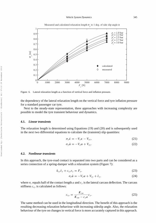
In principle, the stiffness cx and cy could be measured on a non-rolling tyre, but the preferredapproach is to measure the cornering stiffness and lateral relaxation length in a transient test fora number of different inflation pressures and vertical loads. Subsequently, the lateral stiffnessequation can be fitted to these measurement points accordingly. Figure 6 gives an impression of



0 1000 2000 3000 4000 5000 6000 7000 8000 90000

0.1

0.2

0.3

0.4

0.5

0.6

0.7

0.8

0.9

1

Fz [N]

σ y [m

]

Measured and calculated relaxation length σy to 1 deg. of side slip angle α

pi = 1.9 bar

pi = 2.2 bar

pi = 2.5 bar

pi = 2.7 bar

pi = 3.0 bar

calculated

measured

Figure 6. Lateral relaxation length as a function of vertical force and inflation pressure.

the dependency of the lateral relaxation length on the vertical force and tyre inflation pressurefor a standard passenger car tyre.

Next to the steady-state representation, three approaches with increasing complexity arepossible to model the tyre transient behaviour and dynamics.

4.1. Linear transients

The relaxation length is determined using Equations (19) and (20) and is subsequently usedin the next two differential equations to calculate the (transient) slip quantities:

σxκ̇ = −Vxκ − Vsx, (21)

σyα̇ = −Vxα + Vsy. (22)

4.2. Nonlinear transients

In this approach, the tyre-road contact is separated into two parts and can be considered as aseries connection of a spring-damper with a relaxation system (Figure 7):

kcy ε̇y + ccyεy = Fy, (23)

σcα̇ = −Vxα + Vsy + ε̇y, (24)

where σc equals half of the contact length a and εy is the lateral carcass deflection. The carcassstiffness ccy is calculated as follows:

ccy = Kyα

Kyα − cyacy. (25)

The same method can be used in the longitudinal direction. The benefit of this approach is theresulting decreasing relaxation behaviour with increasing sideslip angle. Also, the relaxationbehaviour of the tyre on changes in vertical force is more accurately captured in this approach.



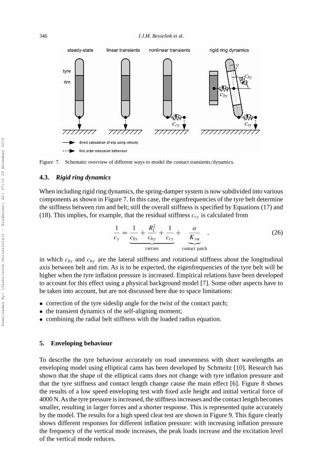
Figure 7. Schematic overview of different ways to model the contact transients/dynamics.

4.3. Rigid ring dynamics

When including rigid ring dynamics, the spring-damper system is now subdivided into variouscomponents as shown in Figure 7. In this case, the eigenfrequencies of the tyre belt determinethe stiffness between rim and belt; still the overall stiffness is specified by Equations (17) and(18). This implies, for example, that the residual stiffness cry is calculated from

1

cy

= 1

cby

+ R2l

cbγ

+ 1

cry︸︷︷︸carcass

+ a

Kyα︸︷︷︸contact patch

, (26)

in which cby and cbγ are the lateral stiffness and rotational stiffness about the longitudinalaxis between belt and rim. As is to be expected, the eigenfrequencies of the tyre belt will behigher when the tyre inflation pressure is increased. Empirical relations have been developedto account for this effect using a physical background model [7]. Some other aspects have tobe taken into account, but are not discussed here due to space limitations:

• correction of the tyre sideslip angle for the twist of the contact patch;• the transient dynamics of the self-aligning moment;• combining the radial belt stiffness with the loaded radius equation.

5. Enveloping behaviour

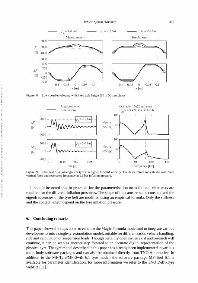
To describe the tyre behaviour accurately on road unevenness with short wavelengths anenveloping model using elliptical cams has been developed by Schmeitz [10]. Research hasshown that the shape of the elliptical cams does not change with tyre inflation pressure andthat the tyre stiffness and contact length change cause the main effect [6]. Figure 8 showsthe results of a low speed enveloping test with fixed axle height and initial vertical force of4000 N.As the tyre pressure is increased, the stiffness increases and the contact length becomessmaller, resulting in larger forces and a shorter response. This is represented quite accuratelyby the model. The results for a high speed cleat test are shown in Figure 9. This figure clearlyshows different responses for different inflation pressure: with increasing inflation pressurethe frequency of the vertical mode increases, the peak loads increase and the excitation levelof the vertical mode reduces.



3000

4000

5000

6000Measurements Simulations

−0.1 −0.05 0 0.05 0.1−500

−250

0

250

500

x [m]−0.1 −0.05 0 0.05 0.1

x [m]

ΔFx

[N]

Fz

[N]

pi = 1.8 bar p

i = 2.2 bar p

i = 2.6 bar

Figure 8. Low speed enveloping with fixed axle height (10 × 50 mm cleat).

ΔFz

[N]

ΔFz

[N]

√PSD[N/√Hz]

√PSD[N/√Hz]

]zH[ycneuqerf]s[emit

MeasurementsSimulations F

z0 = 4.8 kN; V = 30 km/h

Obstacle: 10x20mm cleat

−2000

0

2000 pi = 2.5 bar

0

50

100

0.1 0.15 0.2 0.25−2000

0

2000 pi = 3.0 bar

0 50 100 1500

50

100

Figure 9. Cleat test of a passenger car tyre at a higher forward velocity. The dashed lines indicate the maximumvertical force and resonance frequency at 2.5 bar inflation pressure.

It should be noted that in principle for the parameterisation no additional cleat tests arerequired for the different inflation pressures. The shape of the cams remains constant and theeigenfrequencies of the tyre belt are modified using an empirical formula. Only the stiffnessand the contact length depend on the tyre inflation pressure.

6. Concluding remarks

This paper shows the steps taken to enhance the Magic Formula model and to integrate variousdevelopments into a single tyre simulation model, suitable for different tasks: vehicle handling,ride and calculation of suspension loads. Though certainly open issues exist and research willcontinue, it can be seen as another step forward to an accurate digital representation of thephysical tyre. The tyre model described in this paper has already been implemented in variousmulti-body software packages and can also be obtained directly from TNO Automotive. Inaddition to the MF-Tyre/MF-Swift 6.1 tyre model, the software package MF-Tool 6.1 isavailable for parameter identification, for more information we refer to the TNO Delft-Tyrewebsite [11].



References

[1] H.B. Pacejka, Tyre and Vehicle Dynamics, 2nd ed., Butterworth-Heinemann, Oxford, UK, 2006, ISBN-13:980-0-7506-6918-4.

[2] TNO, MF-Tyre User Manual Version 5.2, 2001[3] E.J.H. de Vries, Motorcycle Tyre Measurements and Models, Proceedings of the 15th symposium Dynamics of

Vehicles on Road and Tracks, IAVSD, Budapest, August 1997.[4] J.J.M. van Oosten, C. Savi, M. Augustin, O. Bouhet, J. Sommer, and J.P. Colinot, TiMe, TIre MEasurements

forces and moments: a new standard for steady state cornering tire testing, EAEC Conference, Barcelona, 30June to 2 July, 1999.

[5] J.J.M. van Oosten, E. Kuiper, G. Leister, D. Bode, H. Schindler, J. Tischleder, and S. Kohne, A new tyre modelfor TIME measurement data, Tire Technology Expo 2003, Hannover, Germany, 2003.

[6] A.J.C. Schmeitz, I.J.M. Besselink, J. de Hoogh, and H. Nijmeijer, Extending the magic formula and SWIFT tyremodels for inflation pressure changes, Reifen, Fahrwerk, Fahrbahn – VDI Conference, Hannover, Germany,2005, pp. 201–225.

[7] I.B.A. op het Veld, Enhancing the MF-Swift tyre model for inflation pressure changes, DCT Rep. 2007.144,Eindhoven University of Technology, 2007.

[8] TNO, Measurement requirements and TYDEX file generation for MF-Tyre/MF-Swift 6.1.Available at www.delft-tyre.nl

[9] Michelin, The Tyre – Rolling Resistance and Fuel Savings, Société de Technologie Michelin-Ferrand, France,2003, p. 84.

[10] A.J.C. Schmeitz, A semi-empirical three-dimensional model of the pneumatic tyre rolling over arbitrarily unevenroad surfaces, Dissertation, Delft University of Technology, The Netherlands, 2004.

[11] TNO Delft-Tyre website. Available at www.delft-tyre.nl

Appendix. TNO MF-TYRE 6.1 Magic Formula equations

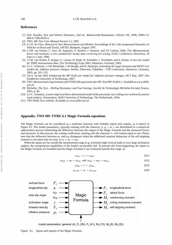
The Magic Formula can be considered as a nonlinear function with multiple inputs and outputs, as is shown inFigure A1. The model parameters, typically starting with the character p, q, r or s, are determined in a numericaloptimisation process minimising the difference between the output of the Magic Formula and the measured forcesand moments. In this process, the scaling coefficients, starting with the character λ, will remain equal to one. Pleasenote that the difference between αF and αM disappears when the additional transient behaviour of the self-aligningmoment is not taken into account, so α = αF = αM.

When the inputs are far outside the measurement range (e.g. extremely high vertical loads or very large inclinationangles), the extrapolation capabilities of the model can possibly fail. To prevent this from happening, the inputs tothe Magic Formula are bounded and the Magic Formula is not evaluated outside this range, so

κmin < κ < κmax, (A1)

αmin < αF < αmax and αmin < αM < αmax, (A2)

γmin < γ < γmax, (A3)

pi,min < pi < pi,max. (A4)

Figure A1. Inputs and outputs of the Magic Formula.



For the vertical force a range is also defined. When the vertical force Fz is outside this range, the Magic Formula isevaluated for the corresponding boundary (Fz,min or Fz,max) when the vertical forces is below Fz,min the resultingforces and moments are scaled with the actual value of the vertical force. A simple example, if the vertical force equals0.5 times Fz,min, then the Magic Formula is evaluated for Fz,min and the resulting forces/moments are multiplied witha factor 0.5. No scaling is applied when the vertical force exceeds forces.

To make the Magic Formula equations dimensionless, the following parameters are introduced:

• unscaled free tyre radius of the non-rolling tyre R0;• nominal vertical force Fz0;• reference forward velocity V0;• nominal tyre inflation pressure pi0.

To account for changes in the vertical force and tyre inflation pressure, dimensionless increments are introduced:

dfz = Fz − Fz0

Fz

, (A5)

dpi = pi − pi0

pi0. (A6)

Many parameters of the MF-Tyre 6.1 tyre model are unchanged and have the same name as in the MF-Tyre 5.2 model.The additional parameter FITTYP has been introduced by TNO to uniquely identify equations. When FITTYP equals61, we are dealing with a MF-Tyre 6.1 dataset.

Al Longitudinal force Fx

Fx = (Dx sin[Cx arctan{Bxκx − Ex(Bxκx − arctan(Bxκx))}] + SV x)Gxα. (A7)

A1.1 Pure slip

κx = κ + SHx, (A8)

Cx = pCx1λCx, (A9)

Dx = μxFz, (A10)

μx = (pDx1 + pDx2 dfz)(1 − pDx3γ

2) (1 + ppx3 dpi + ppx4 dp2

i

)λμx, (A11)

Ex = (pEx1 + pEx2 dfz + pEx3 df2

z

)(1 − pEx4 sgn (κx)) λEx, (A12)

Kxκ = (pKx1 + pKx2 dfz) exp (pKx3 dfz)(1 + ppx1 dpi + ppx2 dp2

i

)FzλKxκ , (A13)

Bx = Kxκ

CxDx

, (A14)

SHx = (pHx1 + pHx2 dfz)λHx, (A15)

SV x = (pV x1 + pV x2 dfz)FzλV xλμx . (A16)

A1.2 Combined slip

Gxα = cos[Cxα arctan{Bxααs − Exα(Bxααs − arctan(Bxααs))}]cos[Cxα arctan{BxαSHxα − Exα(BxαSHxα − arctan(BxαSHxα))}] , (A17)

αs = αF + SHxα, (A18)

Bxα = (rBx1 + rBx3γ2) cos{arctan[rBx2κ]}λxa, (A19)

Cxα = rCx1, (A20)

Exα = rEx1 + rEx2 dfz, (A21)

SHxα = rHx1. (A22)

When combined slip is not used, Gxα = 1.



A2 Lateral force Fy (input αF )

Fy = GyκFyp + SVyκ . (A23)

A2.1 Pure slip

Fyp = Dy sin[Cy arctan

{Byαy − Ey

(Byαy − arctan

(Byαy

))}] + SVy, (A24)

αy = αF + SHy, (A25)

Cy = pCy1λCy, (A26)

Dy = μyFz, (A27)

μy = (pDy1 + pDy2 dfz

) (1 − pDy3γ

2) (1 + ppy3 dpi + ppy4 dp2

i

)λμy, (A28)

Ey = (pEy1 + pEy2 dfz

) (1 + pEy5γ

2 − (pEy3 + pEy4γ

)sgn

(αy

))λEy, (A29)

Kyα = pKy1Fz0(1 + ppy1 dpi

)sin

[pKy4 arctan

{Fz(

pKy2 + pKy5γ 2) (

1 + ppy2 dpi

)Fz0

}] (1 − pKy3 |γ |) λKyα,

(A30)

Kyγ = (pKy6 + pKy7 dfz

) (1 + ppy5 dpi

)FzλKyγ , (A31)

By = Kyα

CyDy

, (A32)

SHy = SHy0 + SHyγ , (A33)

SHy0 = (pHy1 + pHy2 dfz

)λHy, (A34)

SHyγ = Kyγ γ − SVyγ

Kyα

, (A35)

SVy = SVy0 + SVyγ , (A36)

SVy0 = Fz

(pVy1 + pVy2 dfz

)λVyλμy, (A37)

SVyγ = Fz

(pVy3 + pVy4 dfz

)γ λKyγ λμy . (A38)

A2.2 Combined slip

SVyκ = DVyκ sin(rVy5 arctan

(rVy6κ

))λVyκ , (A39)

DVyκ = μyFz

(rVy1 + rVy2 dfz + rVy3γ

)cos

(arctan

(rVy4αF

)), (A40)

Gyκ = cos[Cyκ arctan

{Byκκs − Eyκ

(Byκκs − arctan

(Byκκs

))}]cos

[Cyκ arctan

{ByκSHyκ − Eyκ

(ByκSHyκ − arctan

(ByκSHyκ

))}] , (A41)

κs = κ + SHyκ , (A42)

Byκ = (rBy1 + rBy4γ2) cos{arctan[rBy2(αf − rBy3)]}λyκ , (A43)

Cyκ = rCy1, (A44)

Eyκ = rEy1 + rEy2 dfz, (A45)

SHyκ = rHy1 + rHy2 dfz. (A46)

A3 Overturning moment Mx

Mx = R0FzλMx

{qsx1λV Mx − qsx2γ

(1 + ppmx1 dpi

) + qsx3Fy

Fz0

+ qsx4 cos

[qsx5 arctan

((qsx6

Fz

Fz0

)2)]

· sin

[qsx7γ + qsx8 arctan

(qsx9

Fy

Fz0

)]

+ qsx10 arctan

(qsx11

Fz

Fz0

)γ

}. (A47)



A4 Rolling resistance moment My

My = −R0Fz0λMy

(qsy1 + qsy2

Fx

Fz0+ qsy3

∣∣∣∣Vx

V0

∣∣∣∣ + qsy4

(Vx

V0

)4

+ qsy5γ2 + qsy6

Fz

Fz0γ 2

)

·(

Fz

Fz0

)qsy7(

p

p0

)qsy8

(A48)

When combined slip is not used, SVyκ = 0 and Gyκ = 1.

A5 Self-aligning moment Mz (input αM)

Mz = −tFyp0Gyκ0 + Mzr + sFx, (A49)

where Fyp0Gyκ0 is the combined slip side force with zero inclination angle (γ = 0).

αt = αM + SHt , (A50)

SHt = qHz1 + qHz2 dfz + (qHz3 + qHz4 dfz) γ, (A51)

αr = αM + SHy + SVy

Kyα

, (A52)

A5.1 Pure slip

αt,eq = αt , αr,eq = αr , s = 0. (A53)

A5.2 Combined slip

αt,eq = arctan

√tan2(αt ) +

(Kxκ

Kyα

)2

κ2 · sgn(αt ), (A54)

αr,eq = arctan

√tan2(αr ) +

(Kxκ

Kyα

)2

κ2 · sgn(αr ), (A55)

s =(

ssz1 + ssz2

(Fy

Fz0

)+ (ssz3 + ssz4 dfz) γ

)R0λs, (A56)

A5.3 Pneumatic trail t

t = Dt cos[Ct arctan

{Btαt,eq − Et

(Btαt,eq − arctan

(Btαt,eq

))}]cos (αM) , (A57)

Bt = (qBz1 + qBz2 dfz + qbz3 df2

z

)(1 + qBz4γ + qBz5 |γ |) λKyα

λμy

, (A58)

Ct = qCz1, (A59)

Dt = (qDz1 + qDz2 dfz)(1 − ppz1 dpi

) (1 + qDz3γ + qDz4γ

2) Fz

R0

Fz0λt , (A60)

Et = (qEz1 + qEz2 dfz + qEz3 df2

z

) (1 + (qEz4 + qEz5γ )

(2

π

)arctan (BtCtαt )

). (A61)



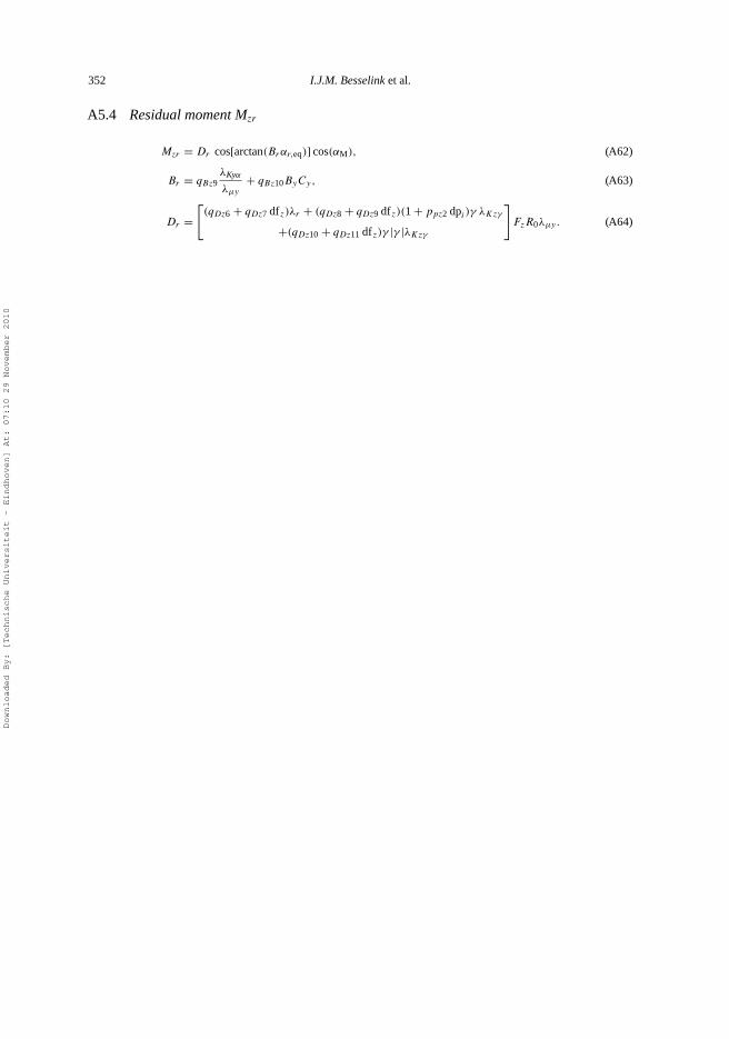
A5.4 Residual moment Mzr

Mzr = Dr cos[arctan(Brαr,eq)] cos(αM), (A62)

Br = qBz9λKyα

λμy

+ qBz10ByCy, (A63)

Dr =[(qDz6 + qDz7 dfz)λr + (qDz8 + qDz9 dfz)(1 + ppz2 dpi )γ λKzγ

+(qDz10 + qDz11 dfz)γ |γ |λKzγ

]FzR0λμy. (A64)


Vehicle System Dynamics An improved Magic Formula…mate.tue.nl/mate/pdfs/12478.pdf · Since its...

Documents

Transcript of Vehicle System Dynamics An improved Magic Formula…mate.tue.nl/mate/pdfs/12478.pdf · Since its...