1

Rule-based Autoregressive Moving Average Models for

Forecasting Load on Special Days: A Case Study for France

Siddharth Arora†and James W. Taylor

*

Saїd Business School,

University of Oxford, Park End Street, Oxford, OX1 1HP, U.K.

European Journal of Operational Research, 2018, Vol. 266, pp. 259-268.

† Siddharth Arora

Tel: +44 (0)1865 288800

Email: Siddharth.Arora@sbs.ox.ac.uk

*James W. Taylor

Tel: +44 (0)1865 288800

Email: James.Taylor@sbs.ox.ac.uk

2

Rule-based Autoregressive Moving Average Models for

Forecasting Load on Special Days: A Case Study for France

___________________________________________________________________________

Abstract

This paper presents a case study on short-term load forecasting for France, with emphasis

on special days, such as public holidays. We investigate the generalisability to French data of

a recently proposed approach, which generates forecasts for normal and special days in a

coherent and unified framework, by incorporating subjective judgment in univariate

statistical models using a rule-based methodology. The intraday, intraweek, and intrayear

seasonality in load are accommodated using a rule-based triple seasonal adaptation of a

seasonal autoregressive moving average (SARMA) model. We find that, for application to

French load, the method requires an important adaption. We also adapt a recently proposed

SARMA model that accommodates special day effects on an hourly basis using indicator

variables. Using a rule formulated specifically for the French load, we compare the SARMA

models with a range of different benchmark methods based on an evaluation of their point

and density forecast accuracy. As sophisticated benchmarks, we employ the rule-based triple

seasonal adaptations of Holt-Winters-Taylor (HWT) exponential smoothing and artificial

neural networks (ANNs). We use nine years of half-hourly French load data, and consider

lead times ranging from one half-hour up to a day ahead. The rule-based SARMA approach

generated the most accurate forecasts.

Keywords: OR in Energy; Load; Short-term; Public holidays; Seasonality.

___________________________________________________________________________

3

1. Introduction

Accurate short-term forecasts of electricity demand (load) are crucial for making

informed decisions regarding unit commitment, energy transfer scheduling, and load-

frequency control of the power system. An electric utility needs to make these operational

decisions on a daily basis, often in real-time, in order to operate in a safe and efficient

manner, optimize operational costs, and improve the reliability of distributional networks.

Moreover, inaccurate forecasts can have substantial financial implications for energy markets

(Weron, 2006).

Given the significance of short-term load forecasts for electric utilities and energy

markets, a plethora of different modelling approaches have been proposed for forecasting

load for normal days (Bunn, 2000). Modelling load for special days, such as public holidays,

however, has usually been overlooked in the research literature (see, for example, Hippert et

al., 2005; Taylor, 2010). Special days exhibit load profiles (shape of the intraday load curve)

that differ noticeably from the repeating seasonal pattern that one might expect. We refer to

load observed on normal days as normal load, whereas load observed on special days is

referred to as anomalous load.

The lack of attention to modelling anomalous load can be attributed to the following: 1)

Anomalous load deviates significantly from normal load, and is therefore not straightforward

to model, as the special days need to be treated as being different from normal days. 2) The

relatively infrequent occurrence of special days results in a lack of anomalous observations

for adequately training the model. 3) Different special days exhibit different load profiles,

which require each special day to be modelled as having a unique profile. The

aforementioned reasons make statistical modelling of anomalous load very challenging, and

this has tended to lead to the forecasting of anomalous load being left to the judgment of the

central controller of the electricity grid (Hyde and Hodenett, 1993, 1997). The aim of this

4

study is to investigate models that can potentially be deployed in a real-time automated online

system, which can assist the central controller in making informed decisions under normal

and anomalous load conditions.

The problem with ignoring anomalous load is that it not only guarantees that the resulting

model cannot be used for special days, but it also results in large forecast errors on normal

days that lie in the vicinity of special days. If special day effects are not modelled, there is

seemingly a need either to replace or smooth observations for these days (see, for example,

Smith, 2000; Hippert et al., 2005; Taylor, 2010; Arora and Taylor, 2016). We use the actual

load time series for modelling, whereby the anomalous observations are neither replaced, nor

smoothed out.

Multivariate weather-based models have been employed previously for modelling load

(Cottet and Smith, 2003; Dordonnat et al., 2008; Cho et al., 2013). Multivariate models

utilize weather variables like temperature, wind speed, cloud cover, and humidity, along with

the historical load observations. Univariate models on the other hand, include only the

historical load observations. It has been argued that the weather variables tend to vary

smoothly over short time scales, and this variation can be captured in the load data itself

(Bunn, 1982). Moreover, for short lead times, univariate models have been shown to be

competitive with weather-based models (Taylor, 2008). In this paper, we employ univariate

methods for short-term load forecasting.

Rule-based forecasting has been proposed as a practical way to incorporate subjective

judgment, based on domain knowledge and expertise, into a statistical model (see, for

example, Armstrong, 2001, 2006). It has been argued that rule-based forecasting can

outperform conventional extrapolation methods, especially in cases where prior domain

knowledge is available and the time series exhibits a consistent structure (see, for example,

Collopy and Armstrong, 1992; Adyaa et al., 2000). Given that the task of forecasting

5

anomalous load has previously relied mainly on subjective judgment, and the fact that load

exhibits a consistent prominent seasonal structure, we adopt a rule-based methodology in this

study. We incorporate domain knowledge into the statistical models via a rule. The rationale

of the proposed rule lies in identifying an historical special day, whose anomalous load

observations would be most useful in improving the accuracy of the model in forecasting load

for the future special day.

In a recent study, Arora and Taylor (2013) propose rule-based approaches for modelling

anomalous load for Great Britain. Of the methods considered, the most successful was based

on SARMA modelling. In this paper, we focus on the use of this method for modelling

French load data. In comparison with load for Great Britain, modelling anomalous load for

France is more challenging, due to the relatively large number of different types of special

days observed in France. As a consequence of this, for the French case, the approach of Arora

and Taylor (2013) requires an adaptation that, although methodologically modest, is

important empirically.

The contributions of this study lie in: 1) Presenting a detailed case study for France,

which focusses on short-term forecasting of anomalous load using a range of different

modelling approaches. 2) Formulating a rule specifically for the French load data that allows

for incorporation of domain knowledge into the statistical framework during the modelling

process. Crucially, the formulated rule treats each special day as having a unique profile,

which may change over the years. The rule categorizes special days into seven different

categories based on an inspection of the anomalous load profiles. 3) Adapting a double

seasonal SARMA method recently proposed in this journal for anomalous load forecasting of

Korean data (see Kim, 2013). In our adaptation of Kim’s method, we treat each special day as

having a unique profile, we incorporate an additional dummy variable in the model to allow

for greater flexibility in accommodating special day effects, and we model triple seasonality.

6

Moreover, we propose a range of different benchmarks for assessing load forecasts on special

days. 4) In addition to generating point forecasts, we evaluate probability density forecasts

across normal and special days. To the best of our knowledge, there are no existing studies on

density forecasting for anomalous load.

In the next section, we present the French load data. In Section 3, we review the literature

on modelling anomalous load. In Section 4, we present the rule-based SARMA method along

with the subjective formulation of a rule. Section 5 presents an adaption of the SARMA

model proposed by Kim (2013). In Section 6, we present the benchmark methods. Empirical

comparison is provided in Section 7. In Section 8, we summarise and conclude the paper.

2. Anomalous Load Characteristics

We employ nine years of half-hourly load for France, stretching from 1 January 2001 to

31 December 2009, inclusive. This leads to a total of 157,776 load observations. We use the

first eight years of the dataset as the estimation sample (consisting of 140,256 observations),

and employ the final year as the evaluation sample (consisting of 17,520 observations). We

generate forecasts by rolling the forecast origin through each half-hour in the post-sample

period. The data has been obtained from Électricité de France (EDF), and there are no

missing observations in the time series. The complete series is presented in Figure 1. It can be

seen from this figure that load exhibits a recurring within-year pattern (due to seasonal

effects), termed the intrayear seasonality. Load in winter is higher than in summer, which is

due to the increased use of electrical equipment for winter heating in France. Also, the data

shows an upward trend.

The average intraday cycle for different days of the week (calculated using only the

estimation sample) is presented in Figure 2. It can be seen from the figure that load on

weekends is considerably lower compared to weekdays, and load is lowest on Sundays. Load

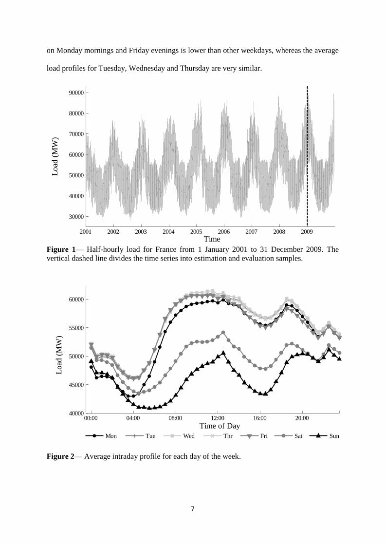
7

on Monday mornings and Friday evenings is lower than other weekdays, whereas the average

load profiles for Tuesday, Wednesday and Thursday are very similar.

Figure 1— Half-hourly load for France from 1 January 2001 to 31 December 2009. The

vertical dashed line divides the time series into estimation and evaluation samples.

Figure 2— Average intraday profile for each day of the week.

2001 2002 2003 2004 2005 2006 2007 2008 2009

30000

40000

50000

60000

70000

80000

90000

Load

(M

W)

Time

00:00 04:00 08:00 12:00 16:00 20:0040000

45000

50000

55000

60000

Time of Day

Load

(M

W)

Mon Tue Wed Thr Fri Sat Sun

8

We identify a total of twenty four special days in the one year post-sample period.

Inspection of the data reveals that load for a given special day is considerably lower than a

normal day, for the same day of the week, around the same date. Figure 3 compares

anomalous and normal load. In this figure, we plot load for Bastille Day in 2008 (14 July

2008), which is a national holiday in France and which fell on a Monday that year. In the

figure, we also plot load for a normal working Monday from the preceding and following

weeks. It is evident from Figure 3 that, not only is anomalous load substantially lower than

normal load, but the shape of the load profiles for normal and special days are indeed very

different. Inspection of the data reveals that this characteristic of anomalous load holds true

across all special days.

Figure 3— Load profile for a Bastille Day, which fell on a Monday (14 July 2008), a normal

Monday (7 July 2008) from the preceding week, and a normal Monday (21 July 2008) from

the following week.

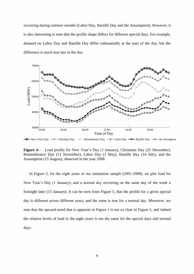
In Figure 4, we plot load profiles for six different special days observed in the year 2008.

As expected, load for special days occurring during winter months (New Year’s Day,

Christmas Day and Remembrance Day) is considerably higher than load for special days

00:00 04:00 08:00 12:00 16:00 20:00

35000

40000

45000

50000

55000

60000

Load

(M

W)

Time of Day

Preceding Normal Monday

Bastille Day (Monday)

Following Normal Monday

9

occurring during summer months (Labor Day, Bastille Day and the Assumption). However, it

is also interesting to note that the profile shape differs for different special days. For example,

demand on Labor Day and Bastille Day differ substantially at the start of the day, but the

difference is much less late in the day.

Figure 4— Load profile for New Year’s Day (1 January), Christmas Day (25 December),

Remembrance Day (11 November), Labor Day (1 May), Bastille Day (14 July), and the

Assumption (15 August), observed in the year 2008.

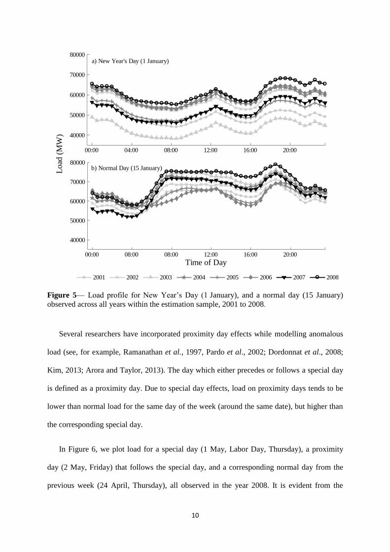
In Figure 5, for the eight years of our estimation sample (2001-2008), we plot load for

New Year’s Day (1 January), and a normal day occurring on the same day of the week a

fortnight later (15 January). It can be seen from Figure 5, that the profile for a given special

day is different across different years, and the same is true for a normal day. Moreover, we

note that the upward trend that is apparent in Figure 1 is not so clear in Figure 5, and indeed

the relative levels of load in the eight years is not the same for the special days and normal

days.

00:00 04:00 08:00 12:00 16:00 20:0030000

40000

50000

60000

70000

Lo

ad (

MW

)

Time of Day

New Years Day Christmas Day Remembrance Day Labor Day Bastille Day the Assumption

10

Figure 5— Load profile for New Year’s Day (1 January), and a normal day (15 January)

observed across all years within the estimation sample, 2001 to 2008.

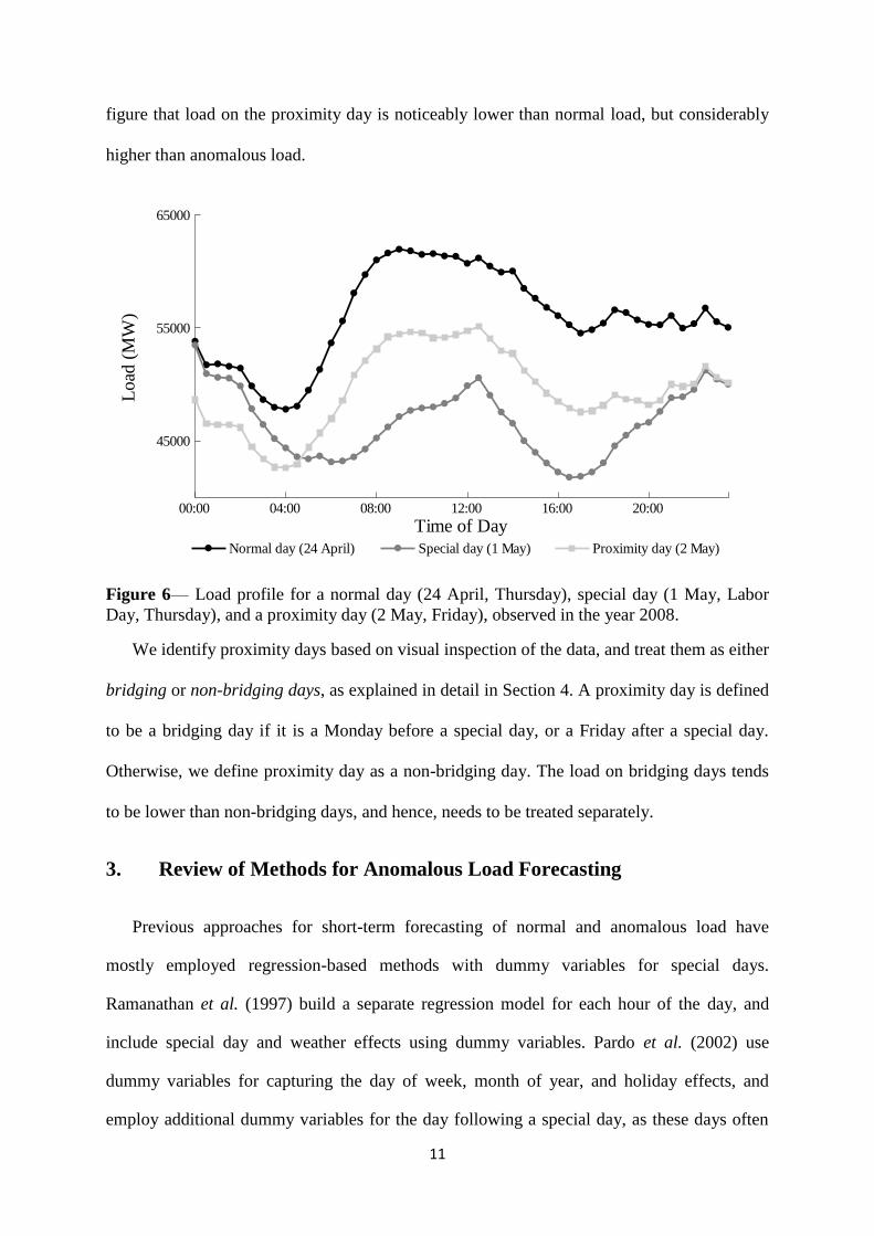
Several researchers have incorporated proximity day effects while modelling anomalous

load (see, for example, Ramanathan et al., 1997, Pardo et al., 2002; Dordonnat et al., 2008;

Kim, 2013; Arora and Taylor, 2013). The day which either precedes or follows a special day

is defined as a proximity day. Due to special day effects, load on proximity days tends to be

lower than normal load for the same day of the week (around the same date), but higher than

the corresponding special day.

In Figure 6, we plot load for a special day (1 May, Labor Day, Thursday), a proximity

day (2 May, Friday) that follows the special day, and a corresponding normal day from the

previous week (24 April, Thursday), all observed in the year 2008. It is evident from the

00:00 04:00 08:00 12:00 16:00 20:00

40000

50000

60000

70000

80000

00:00 08:00 08:00 12:00 16:00 20:00

40000

50000

60000

70000

80000

Time of Day

Lo

ad (

MW

)

2001 2002 2003 2004 2005 2006 2007 2008

a) New Year's Day (1 January)

b) Normal Day (15 January)

11

figure that load on the proximity day is noticeably lower than normal load, but considerably

higher than anomalous load.

Figure 6— Load profile for a normal day (24 April, Thursday), special day (1 May, Labor

Day, Thursday), and a proximity day (2 May, Friday), observed in the year 2008.

We identify proximity days based on visual inspection of the data, and treat them as either

bridging or non-bridging days, as explained in detail in Section 4. A proximity day is defined

to be a bridging day if it is a Monday before a special day, or a Friday after a special day.

Otherwise, we define proximity day as a non-bridging day. The load on bridging days tends

to be lower than non-bridging days, and hence, needs to be treated separately.

3. Review of Methods for Anomalous Load Forecasting

Previous approaches for short-term forecasting of normal and anomalous load have

mostly employed regression-based methods with dummy variables for special days.

Ramanathan et al. (1997) build a separate regression model for each hour of the day, and

include special day and weather effects using dummy variables. Pardo et al. (2002) use

dummy variables for capturing the day of week, month of year, and holiday effects, and

employ additional dummy variables for the day following a special day, as these days often

00:00 04:00 08:00 12:00 16:00 20:00

45000

55000

65000

Load

(M

W)

Time of Day

Normal day (24 April) Special day (1 May) Proximity day (2 May)

12

also exhibit abnormal load patterns. Cottet and Smith (2003) model load using a multi-

equation Bayesian model, whereby they employ 48 coefficients for each dummy variable to

capture the intraday seasonality in their half-hourly load data. Cancelo et al. (2008) build a

separate model for each hour of the day using Spanish load. They first issue a forecast for

load assuming a normal day, and make adjustments accordingly for special days using

different dummy variables employed for different classes of special days. Soares and

Medeiros (2008) build a two-stage model for each hour of the day, such that anomalous load

is modelled in the first stage using dummy variables. Any unexplained component in load is

then modelled in the second stage using either an AR model or an ANN. Dordonnat et al.

(2008) build a regression model for each hour of the day, and accommodate special day

effects using dummy variables. In addition, they also use dummy variables for bridging days.

Gould et al. (2008) propose a state space approach for forecasting time series with multiple

seasonal patterns, and accommodate special day effects by treating them as if they are

Saturdays or Sundays. De Livera et al. (2011) propose an innovations state space modelling

framework, and handle special day effects for national and religious holidays in load via

dummy variables. Kim (2013) employs a double seasonal ARMA model to accommodate

special day effects on an hourly basis using indicator variables for Korean load. In Section 5,

we adapt the method used by Kim (2013) for French load.

For the approach to anomalous load that involves the use of regression models and

dummy variables, to avoid over-parameterisation, different special days have often been

classified as belonging to the same special day type (see, for example, Kim et al., 2000;

Cottet and Smith, 2003; Cancelo et al., 2008; Soares and Medeiros, 2008; Dordonnat et al.,

2008; Kim, 2013). The classification of special days relies on the assumption that the load

profile for different special days can be treated as being similar, and would remain similar

over the years. Using French load, we observe from the data that each special day exhibits a

unique profile, as shown in Figure 4. Hence, instead of classifying different special days as

13

being the same, we model each special day as having a unique profile, which may change

over different years.

Most existing methods for anomalous load forecasting rely on classifying different

special days as being the same, while some approaches employ different models for normal

and special days (Kim et al., 2000). By contrast, Arora and Taylor treat each special day as

having a unique profile, and adopt a unified modelling framework for normal and special

days. In this paper, we adapt and apply the approach of Arora and Taylor to French load.

Apart from regression-based methods, some authors have proposed rule-based approaches

for anomalous load forecasting, while others have used ANNs. Rahman and Bhatnagar

(1988) propose a rule-based approach, whereby they formulate rules based on the logical and

syntactical relationships between weather and load. Hyde and Hodnett (1997) formulate rules

for Irish load data, whereby the rationale of their approach is to find the deviation of load for

different special days from normal load for a given year, and use this deviation as a

correction term for the corresponding special day falling next year. Kim et al. (2000) classify

special days into five different types, and employ an ANN (for each special day type) used in

conjunction with fuzzy rules inferred from their Korean load data. Recently, Barrow and

Kourentzes (2016) proposed ANNs for accommodating the effect of special days while

modelling call centre arrivals. Using load time series for Great Britain, Arora and Taylor

(2013) demonstrate how a set of univariate methods can be adapted to model load for special

days, when used in conjunction with a rule-based approach.

The existing rule-based methods are tailored only to the data at hand (Rahman and

Bhatnagar, 1988; Hyde and Hodnett, 1993, 1997). This makes the task of adapting existing

rule-based methods to different datasets very challenging, and would require, for these rule-

based methods, creating a completely new set of rules for the French data. For this reason, we

do not use existing rule-based methods as benchmark methods in this study.

14

4. Rule-based Modelling Framework

This section presents a rule-based SARMA method, along with the principles of

formulating a rule based on a categorization of special days. Our methodological contribution

to this section is to provide an important adaption of the rule for application to the French

case.

4.1. Rule-based SARMA

In this paper, for the French load data, we consider the rule-based adaptation of SARMA

proposed by Arora and Taylor (2013) for modelling anomalous load. The model has the

following formulation:

𝛶𝑝(𝐿)𝛷𝑃1(𝐿𝑚1)𝛸𝑃2

(𝐿𝑚2) (𝐼𝑁𝑡𝛹(𝐿𝑚3(𝑡))+(1 − 𝐼𝑁𝑡

)𝜃(𝐿𝑚3(𝑡))) (𝑦𝑡 − 𝑐) =

𝛺𝑞(𝐿)𝛩𝑄1(𝐿𝑚1)𝛤𝑄2

(𝐿𝑚2) (𝐼𝑁𝑡𝛬(𝐿𝑚3(𝑡))+(1 − 𝐼𝑁𝑡

)𝛫(𝐿𝑚3(𝑡))) (𝐼𝑁𝑡𝜀𝑡

(𝑁)+(1 − 𝐼𝑁𝑡

)𝜀𝑡(𝑆)

)

(1)

where 𝑦𝑡 denotes the load observed at period 𝑡, 𝑐 is a constant parameter; 𝐿 denotes a lag

operator; and 𝛶𝑝, 𝛷𝑃1and 𝛸𝑃2

are AR polynomial functions of order 𝑝, 𝑃1 and 𝑃2, while 𝛺𝑞,

𝛩𝑄1 and 𝛤𝑄2

are MA polynomial functions of order 𝑞, 𝑄1 and 𝑄2, respectively. We consider

polynomial function orders equal to or less than three. The model errors for normal and

special days are denoted by 𝜀𝑡(𝑁)

~𝑁𝐼𝐷(0, 𝜎𝑁2) and 𝜀𝑡

(𝑆)~𝑁𝐼𝐷(0, 𝜎𝑆

2) , respectively, having

corresponding variances 𝜎𝑁2 and 𝜎𝑆

2 , while 𝑁𝐼𝐷 refers to a normal and independently

distributed process. For any period 𝑡 occurring on a normal day, the binary indicator 𝐼𝑁𝑡

equals one, and zero otherwise.

The length of the intraday, intraweek, and intrayear seasonal cycle are denoted by 𝑚1,

𝑚2 and 𝑚3(𝑡). Since the data is recorded every half-hour, we have 𝑚1 = 48 and 𝑚2 = 336.

For normal days, we have 𝑚3(𝑡) = 52 × 𝑚2 (for a given period 𝑡), except for a few weeks

around the clock-change, where 𝑚3(𝑡) = 53× 𝑚2. (Clock-change involves the clocks being

15

put forward by an hour on the last Sunday in March, and put back one hour on the last

Sunday in October.) For special days, it is very important to note that 𝑚3(𝑡) is selected using

a rule-based approach, which we describe in detail later in this section. We refer to this model

as rule-based triple seasonal autoregressive moving average (RB-SARMA).

In expression (1), the functions 𝛹 and 𝛬 accommodate the intrayear seasonal effects for

normal days; while 𝜃 and 𝛫 accommodate intrayear seasonality for special days. The

function 𝛹 is written as:

𝛹(𝐿𝑚3(𝑡)) = 1 + 𝜂1𝐿𝑚3(𝑡) + 𝜂2𝐿𝑚3(𝑡)+𝑚3(𝑡−𝑚3(𝑡)) + 𝜂3𝐿𝑚3(𝑡)+𝑚3(𝑡−𝑚3(𝑡))+𝑚3(𝑡−𝑚3(𝑡−𝑚3(𝑡)))

(2)

where 𝜂1, 𝜂2 and 𝜂3 are constant parameters. The functions 𝜃, 𝛬 and 𝛫 are of the same form

as 𝛹, with the difference that each function involves a different set of parameters. With these

functions, the formulation in expression (1) involves switching between different AR and

MA polynomial functions, with different annual lag terms, depending on whether 𝑦𝑡 belongs

to a normal day, or a special day. We adopt the Box and Jenkins (1970) methodology to

select the orders for all the polynomial functions in expression (1).

The model parameters for RB-SARMA are estimated by maximum likelihood, employing

only the in-sample data. The likelihood function assumes a Gaussian error, for which the

variance is different on special days to that of normal days. Specifically, we use the following

log-likelihood (LL) function:

𝐿𝐿 = −𝑛𝑁𝐷

2log(2𝜋𝜎𝑁

2) −𝑛𝑆𝐷

2log(2𝜋𝜎𝑆

2)

− ∑ (𝐼𝑁𝑡

2𝜎𝑁2 (𝜀𝑡

(𝑁))2 +

(1 − 𝐼𝑁𝑡)

2𝜎𝑆2 (𝜀𝑡

(𝑆))2)

𝑁

𝑡=365×𝑚1+1

(3)

where 𝑁 is the length of the estimation sample, 𝑛𝑁𝐷 and 𝑛𝑆𝐷 are the number of load

observations that belong to normal and special days, respectively, excluding the observations

from the first year. To estimate model parameters, we used an optimization scheme based on

a simplex search method of Lagarias et al. (1998). Once estimated, the parameters were held

16

fixed, and the estimated model was employed for generating forecasts for the out-of-sample

data.

4.2. Rule Formulation: Principles

The RB-SARMA method described in Section 4.1 requires the value of the intrayear

cycle length, 𝑚3(𝑡), to be specified for each period 𝑡 in the estimation sample, and each

period for which a forecast is required. For normal days, as we stated in Section 4.1, 𝑚3(𝑡) is

set to be either 52 × 𝑚2 or 53 × 𝑚2 (depending on the proximity of 𝑡 to the clock-change).

For special days, each value for 𝑚3(𝑡) is essentially chosen subjectively. This subjectivity is

supported by a rule-based framework, which is the focus of this section. The important point

to appreciate is that the sole purpose of the rule is to determine, for each special day, the

value of 𝑚3(𝑡). In our description of the rule, we refer to the day on which period 𝑡 falls as

the current special day, and the day on which 𝑡-𝑚3(𝑡) falls as the corresponding past special

day.

The rule considered in this study is an adaptation of a rule proposed by Arora and Taylor

(2013). In that study, four different rules were proposed for a British load time series. Of the

four rules, Rule 3 performed the best for special days. In this paper, we focus on this one rule,

and adapt it for the relatively large number of different types of special days observed in

France. We ensure that the rule treats each special day as having a unique profile.

Specifically, for each special day, 𝑚3(𝑡) is chosen in accordance with the following

principles:

(i) 𝑚3(𝑡) is chosen to be a multiple of 𝑚1, which is equal to 48 for our French data. This

seems intuitively reasonable, as it ensures that 𝑚3(𝑡) relates each period in the current special

day to the same period of the day in the corresponding past special day.

17

(ii) 𝑚3(𝑡) is chosen to be the same for all periods 𝑡 on the current special day. This means

that, for each current special day, the rule prescribes a single corresponding past special day.

(iii) Figure 2 shows that the average intraday load profile for weekends is substantially lower

compared to weekdays. In view of this, for each special day, 𝑚3(𝑡) is chosen so that the

current day and corresponding past day are either both weekdays, or both fall on weekends.

(iv) When choosing between two past special days from different years, to use as the

corresponding past special day, select the one from the most recent of the two years.

(v) The corresponding past special day should be chosen so that it occurs at a similar time of

year to the current special day. For some special days, the date of current and corresponding

past special days should be the same. For others, it is more important that the day of the week

is the same. The difference in how the corresponding past special day should be selected

leads us to categorise the special days into one of seven different special day types.

Specifically, it is important to note that to model load for a given special day, we refer to the

most recent past special day that belongs to the same category as the special day under

consideration. In defining these categories, we incorporate all of the principles described in

this section. We present the seven categories in Section 4.3.

4.3. Rule Formulation: Special Day Categories

Table 1 presents the special days of 2009, with each allocated to one of the seven

categories of special day types. For each special day in 2009, the table also shows the

corresponding past special day. In this section, we describe the categorization of special days.

We define the national public holidays as basic special days. Each seems to have a

somewhat different load profile to any other special day, and so in defining 𝑚3(𝑡), it seems

sensible to relate each of these special days to the same special day occurring in the past.

With patterns of load on weekdays being very different to patterns on weekends, if the

18

current basic special day falls on a weekday, 𝑚3(𝑡) is chosen so that the corresponding past

day is chosen as the most recent occurrence of the same special day that fell on a weekday.

Similarly, if the current basic special day falls on a weekend, 𝑚3(𝑡) is set in order that the

corresponding past day is chosen as the most recent occurrence of the same special day that

fell on a weekend. This leads us to the following two categories of special days:

Category A: Basic special days that occur on a weekday.

Category B: Basic special days that occur on a weekend.

For 2009, Table 1 presents the 10 special days in Category A and the 3 special days in

Category B, and their corresponding past special days.

As we explained in Section 2, a proximity day is a special day that either precedes or

follows a basic special day. Load on all proximity days is sufficiently abnormal that it is

necessary to treat them as special days. The pattern of load on a proximity day that follows a

special day is typically different to the load profiles for proximity days that precede a special

day. This is reflected in the categorization. Furthermore, the categorization also accounts for

proximity days that are bridging days. As described in Section 2, a bridging day is a

proximity day that occurs between a special day and a weekend. Load on a bridging day

tends to be lower than on non-bridging proximity days. Considerations regarding proximity

days lead us to the following five categories of special days:

Category C: Bridging proximity days that precede a special day.

Category D: Bridging proximity days that follow a special day.

Category E: Non-bridging proximity days that precede a special day, and occur on a

weekday.

Category F: Non-bridging proximity days that follow a special day, and occur on a weekday.

Category G: Non-bridging proximity days that follow a special day, and occur on a

weekend.

19

TABLE 1: CATEGORISATION OF FRENCH SPECIAL DAYS IN 2009, AND THE

CORRESPONDING PAST SPECIAL DAY SELECTED TO DEFINE 𝑚3(𝑡).

Current Special Day :

Corresponding Past Special Day Referred

to via 𝒎𝟑(𝒕)

Category A: Basic special days that occur on a weekday

New Year’s Day : Thu 01/01/2009 New Year's Day : Tue 01/01/2008

Easter Monday : Mon 13/04/2009 Easter Monday : Mon 24/03/2008

Labor Day : Fri 01/05/2009 Labor Day : Thu 01/05/2008

WWII Victory Day : Fri 08/05/2009 WWII Victory Day : Thu 08/05/2008

Ascension Day : Thu 21/05/2009 Ascension Day : Thu 17/05/2007

Whit Monday : Mon 01/06/2009 Whit Monday : Mon 12/05/2008

Bastille Day : Tue 14/07/2009 Bastille Day : Mon 14/07/2008

Remembrance Day : Wed 11/11/2009 Remembrance Day : Tue 11/11/2008

Christmas Day : Fri 25/12/2009 Christmas Day : Thu 25/12/2008

New Year’s Eve : Thu 31/12/2009 New Year’s Eve : Wed 31/12/2008

Category B: Basic special days that occur on a weekend

* The Assumption : Sat 15/08/2009 The Assumption : Fri 15/08/2008

All Saints Day : Sun 01/11/2009 All Saints Day : Sat 01/11/2008

Boxing Day : Sat 26/12/2009 Boxing Day : Sun 26/12/2004

Category C: Bridging proximity days that precede a special day **

Day before Bastille Day : Mon 13/07/2009 Day after Bastille Day : Fri 15/07/2005

Category D: Bridging proximity days that follow a special day

Day after New Year's : Fri 02/01/2009 Day after New Year's : Fri 02/01/2004

Day after Ascension : Fri 22/05/2009 Day after Ascension : Fri 18/05/2007

Category E: Non-bridging proximity days that precede a special day, and occur on a weekday

Christmas Week : Mon 21/12/2009 Christmas Week : Mon 22/12/2008

Christmas Week : Tue 22/12/2009 Christmas Week : Mon 22/12/2008

Christmas Week : Wed 23/12/2009 Christmas Week : Tue 23/12/2008

Christmas Week : Thu 24/12/2009 Christmas Week : Wed 24/12/2008

Category F: Non-bridging proximity days that follow a special day, and occur on a weekday

Christmas Week : Mon 28/12/2009 Christmas Week : Mon 29/12/2008

Christmas Week : Tue 29/12/2009 Christmas Week : Mon 29/12/2008

Christmas Week : Wed 30/12/2009 Christmas Week : Tue 30/12/2008

Category G: Non-bridging proximity days that follow a special day, and occur on a weekend

Christmas Week : Sun 27/12/2009 Christmas Week : Sat 30/12/2006

* The Assumption in 2009 occurred on a weekend (Saturday), however, there were no instances of this basic special day falling on a

weekend in the estimation period, hence, for this case, we simply refer to the profile of the same special day from the previous year (2008).

** For the bridging proximity day that preceded Bastille Day in 2009 (Monday), we did not have an instance of a corresponding past bridging proximity day that preceded Bastille Day and fell on same day of the week (Monday), hence, for this case, we simply refer to the

profile of a past bridging proximity day that follows Bastille Day.

20

Let us provide an illustrative example of the specification of 𝑚3(𝑡) for a proximity day.

Let us consider Friday 22 May 2009. This day is allocated to Category D, because it is a

Friday following Ascension Day (Thursday 21 May 2009). The rule requires us to select, as

corresponding past special day, the special day in Category D that occurred at the same time

of year, most recently. This leads to the choice of Friday 18 May 2007, as the corresponding

past special day, because Ascension Day occurred on 17 May in 2007. Hence, for all periods

on Friday 22 May 2009, we set 𝑚3(𝑡) = (365 + 366 + 4) × 48 . In cases where the

magnitude of 𝑚3(𝑡) is larger than the total number of historical observations, the

corresponding special day is set as the same special day from the previous year.

5. SARMA with Indicator Variables for Special Days

In a recent study in this journal, Kim (2013) used a SARMAX model (double seasonal

ARMA with indicator variables) to forecast anomalous load. Specifically, Kim (2013)

employed two types of indicator variables (denoted by 𝐴ℎ,𝑡 and 𝐵ℎ,𝑡 ) in the SARMAX

modelling framework. The variable 𝐴ℎ,𝑡 was an indicator variable used to indicate whether

load observed on intraday period h on a special day (for a given period 𝑡) deviates from

normal load, whereas 𝐵ℎ,𝑡 was employed to quantify the extent of this deviation.

Kim (2013) treated different special days as being the same, with one variable (𝐵ℎ,𝑡) to

distinguish between different levels of deviation between normal and anomalous load. In this

study, we implement an adaptation of the model, which, in our empirical analysis, improved

forecast accuracy considerably. In our adaptation, we: 1) treat each special day as having a

unique profile; 2) employ an additional indicator variable (𝐶𝑡) to enable greater flexibility in

accommodating the special day effects; and 3) model triple seasonality. We refer to the

adapted model as SARMAX(ABC), and formulate it as:

21

𝑦𝑡 = 𝑐 + ∑ 𝛼ℎ𝐴ℎ,𝑡

𝑚1

ℎ=1

+ ∑ 𝛽ℎ𝐵ℎ,𝑡

𝑚1

ℎ=1

+ ∑ 𝛾ℎ𝐶ℎ,𝑡

𝑚1

ℎ=1

+𝛺𝑞(𝐿)𝛩𝑄1

(𝐿𝑚1)𝛤𝑄2(𝐿𝑚2)𝛬(𝐿𝑚3(𝑡))

𝛶𝑝(𝐿)𝛷𝑃1(𝐿𝑚1)𝛸𝑃2

(𝐿𝑚2)𝛹(𝐿𝑚3(𝑡))(𝐼𝑁𝑡

𝜀𝑡(𝑁)

+(1 − 𝐼𝑁𝑡)𝜀𝑡

(𝑆))

(4)

where h is counter for the 𝑚1 periods of in each day; 𝛼ℎ, 𝛽ℎ and 𝛾ℎ are the model parameters;

𝐴ℎ,𝑡 , 𝐵ℎ,𝑡 and 𝐶ℎ,𝑡 are the indicator variables. For normal and anomalous periods, we use

𝑚3(𝑡) = 52 × 𝑚2 (except for a few weeks around clock-change, where 𝑚3(𝑡) = 53 × 𝑚2).

The remaining terms for SARMAX(ABC) are as defined earlier for RB-SARMA.

To understand the indicator variables, 𝐴ℎ,𝑡, 𝐵ℎ,𝑡 and 𝐶ℎ,𝑡, first note that each is equal to

zero if period t does not occur on intraday period h. If period t does fall on intraday period h,

the indicator variables take a value of 1 if that period is deemed to differ notably from what

one might expect. The indicator variable values for all anomalous periods in 2009 are

provided in Table 2.

To explain the indicator variable coding scheme more precisely, for load observed on a

given special day (𝑦𝑡), we refer to load observed on the same special day from the last year

(denoted by 𝑦𝑡−𝑚3′ (𝑡)). We compute the percentage difference between 𝑦𝑡−𝑚3

′ (𝑡) and the mean

of the previous 4 corresponding periods on normal days that fell on same day of the week

(µ𝑡 =1

4∑ 𝑦𝑡−𝑚3

′ (𝑡)−𝑖×𝑚1

4𝑖=1 ). Kim (2013) set 𝐵ℎ,𝑡=1, if the percentage difference was between

10% and 20%, and 𝐵ℎ,𝑡=2, if the percentage difference was greater than 20%, but we found

this to be overly restrictive, and hence we included a third indicator variable 𝐶ℎ,𝑡. We set

𝐴ℎ,𝑡=1 if the percentage difference is at least 10%; we set 𝐵ℎ,𝑡=1 if the percentage difference

is between 10% and 20%; and we set 𝐶ℎ,𝑡=1 if the percentage difference is more than 20%.

22

TABLE 2: CATEGORISATION OF FRENCH SPECIAL DAYS IN 2009, AND THE VALUE OF

CORRESPONDING INDICATOR VARIABLES FOR DIFFERENT PERIODS OF THE DAY.

Current Special Day :

Intraday periods on which indicator variables are 1

Category A: Basic special days that occur on a weekday 𝐴ℎ,𝑡 = 1; 𝐵ℎ,𝑡 = 1 𝐴ℎ,𝑡 = 1; 𝐶ℎ,𝑡 = 1

New Year’s Day : Thu 01/01/2009 05:30-06:30, 10:30-19:00 -

Easter Monday : Mon 13/04/2009 - -

Labor Day : Fri 01/05/2009 02:30-05:00, 21:00-23:30 05:30-20:30

WWII Victory Day : Fri 08/05/2009 00:00-02:00, 21:30-23:30 02:30-21:00

Ascension Day : Thu 21/05/2009 02:30-05:00, 21:00-23:30 05:30-20:30

Whit Monday : Mon 01/06/2009 00:00-03:00, 21:30-23:30 04:00-21:00

Bastille Day : Tue 14/07/2009 05:00-06:00, 12:30, 06:30-12:00,

19:30-23:00 13:00-19:00

Remembrance Day : Wed 11/11/2009 05:30-06:30, 09:00-17:00 07:00-08:30

Christmas Day : Fri 25/12/2009 01:00-05:00, 20:00-23:30 05:30-19:30

New Year’s Eve : Thu 31/12/2009 - -

Category B: Basic special days that occur on a weekend

The Assumption : Sat 15/08/2009 00:00-06:00, 19:30-23:30 06:30-19:00

All Saints Day : Sun 01/11/2009 - -

Boxing Day : Sat 26/12/2009 00:00-10:30 -

Category C: Bridging proximity days that precede a special day Day before Bastille Day : Mon 13/07/2009 - -

Category D: Bridging proximity days that follow a special day

Day after New Year's : Fri 02/01/2009 - -

Day after Ascension : Fri 22/05/2009 00:00-23:30 -

Category E: Non-bridging proximity days that precede a special day, and occur on a weekday

Christmas Week : Mon 21/12/2009 - -

Christmas Week : Tue 22/12/2009 - -

Christmas Week : Wed 23/12/2009 05:00-23:00 -

Christmas Week : Thu 24/12/2009 00:00-23:30 -

Category F: Non-bridging proximity days that follow a special day, and occur on a weekday

Christmas Week : Mon 28/12/2009 00:00-23:30 -

Christmas Week : Tue 29/12/2009 - -

Christmas Week : Wed 30/12/2009 - -

Category G: Non-bridging proximity days that follow a special day, and occur on a weekend

Christmas Week : Sun 27/12/2009 06:30-07:30 -

Note: As expected, the indicator variables (𝐴ℎ,𝑡, 𝐵ℎ,𝑡 and 𝐶ℎ,𝑡) are non-zero for most periods on basic special days. This variable coding

scheme reflects that load observed on basic special days is considerably lower compared to load observed on normal days and proximity

days.

23

6. Benchmark Methods

We present five simple benchmarks in Section 6.1. In addition, as sophisticated

benchmarks, we present Arora and Taylor’s (2013) rule-based adaptations of Holt-Winters-

Taylor (HWT) exponential smoothing and artificial neural networks (ANNs) in Section 6.2

and Section 6.3, respectively.

6.1. Simple Benchmarks

We consider five simple benchmark methods to model load for a given special day, we

use: 1) Recent Sunday – load observed on the most recent Sunday. This benchmark method

was employed by Smith (2000).

2) Seasonal random walk (SRW) – load observed on the same special day in the last year.

3) Seasonal random walk for same day of the week (SRW-Day) – load observed on the

same special day in a past year, with the year chosen as the most recent year in which both

current and previous special days occur on the same day of the week.

4) Seasonal random walk for weekday/weekend (SRW-WkDay/WkEnd) – load observed

on the same special day in a past year, with the year chosen as the most recent year in which

both current and previous special days belong either to a weekday, or a weekend. This

benchmark method is based on the rule presented in Section 4.

5) Seasonal random walk for same intraday cycle (SRW-IC) – load observed on the same

special day in a past year, with the year chosen as the most recent year in which both current

and previous special days belong to the same intraday cycle. Following Taylor (2010), we

treat a week as comprising five different intraday cycles.

6.2. Rule-based HWT

In this paper, we implement the rule-based HWT exponential smoothing method,

proposed by Arora and Taylor (2013) for normal and anomalous load. This method focuses

24

on modelling anomalous load in terms of its deviation from normal load. Specifically, to

model French load for special days, the method employs the daily and weekly seasonal

indices for normal days, and adjusts the anomalous load profile accordingly for special days

using the annual seasonal index. A single source of error state space model is used, which

requires the estimation of smoothing parameters for the level, intraday, intraweek and

intrayear seasonal indices, along with a parameter that adjusts for first order autocorrelation

in the error. The smoothing parameters determine the rate at which the level and seasonal

indices are updated. Observations from the first year in the training set are used to initialize

the level and seasonal indices. The value of 𝑚3(𝑡) is selected using the same rule-based

approach for special days, as used in the RB-SARMA method. The model parameters are

estimated by maximum likelihood, employing the same optimization scheme and log

likelihood expression used for the RB-SARMA method, whereby we use different variances

for model errors for normal and special days. We refer to this method as RB-HWT.

6.3. Rule-based ANN

ANNs have been widely used for modelling anomalous load (see, for example, Kim et al.,

2000; Hippert et al., 2005). In this study, we employ a feed-forward ANN method with a

single hidden layer and a single output, as used by Arora and Taylor (2013). We pre-process

the load data prior to modelling, using a double differencing operator of the form (1 −

𝐿𝑚1)(1 − 𝐿𝑚2) . We difference the load data using this operator, and normalize it by

subtracting the mean, and dividing by the standard deviation. We used this variable as output,

and we used lagged values of the output as inputs to the ANN. As ANNs have been shown to

be unsuitable for generating multi-step ahead forecasts (Atiya et al., 1999), we build a

separate ANN model for each forecast horizon. We selected the lags for the input variables to

be as consistent as possible with the SARMA model. Using a rule-based ANN, we model the

normal and special days in a unified framework. The rule-based approach avoids the

25

complexity of employing separate ANNs for different types of special days and normal days.

The value of 𝑚3(𝑡) is selected using the rule-based approach for special days, as used in RB-

SARMA and RB-HWT. We estimate the model parameters using cross-validation, employing

a hold-out sample corresponding to the last one year of the estimation sample. To estimate

the link weights, we used least squares with backpropagation. We choose the activation

functions for the hidden and output layer to be sigmoid and linear, respectively. We selected

the input variables, number of units in the hidden layer, backpropagation learning rate and

momentum parameters, and regularization parameters using only the cross-validation hold-

out data. We refer to this method as RB-ANN.

7. Empirical Comparison

We provide an empirical comparison of the methods discussed in Sections 4, 5 and 6,

based on an evaluation of their point and density forecast accuracy for the post-sample

period, which consists of all half-hours in 2009. In our discussion of the results, we use the

terminology, SARMA, HWT and ANN to refer to the original versions of the SARMA

method, HWT exponential smoothing, and ANNs, respectively. These methods make no

attempt to model the special days, and are presented by Taylor (2010). As we indicated

previously, we refer to the corresponding rule-based method as RB-SARMA, RB-HWT and

RB-ANN, respectively. Moreover, we refer to the SARMA method with indicator variables

for special days as SARMAX(ABC). In Section 7.1, we consider point forecasting, and then

discuss density forecasting in Section 7.2.

7.1. Point Forecasting

To evaluate point forecasts, we use the Mean Absolute Percentage Error (MAPE) and

Root Mean Squared Percentage Error (RMSPE). The relative model rankings were similar for

the two measures; hence, we present results using only the MAPE in this paper.

26

TABLE 3: MAPE ACROSS ONLY SPECIAL DAYS FOR FIVE SIMPLE BENCHMARKS, TWO

SOPHISTICATED BENCHMARKS, AND THE ORIGINAL VERSION AND RULE-BASED

ADAPTATION OF SARMA, AND SARMAX (ABC).

Horizon (in hours) 1-3 4-6 7-9 10-12 13-15 16-18 19-21 22-24

Simple benchmarks

Recent Sunday 11.66 11.66 11.65 11.65 11.65 11.65 11.68 11.71

SRW 10.49 10.51 10.53 10.56 10.58 10.61 10.63 10.65

SRW-Day 11.72 11.73 11.75 11.77 11.79 11.81 11.83 11.84

SRW-WkDay/WkEnd 10.09 10.11 10.13 10.15 10.18 10.20 10.23 10.25

SRW-IC 10.98 11.00 11.02 11.05 11.07 11.10 11.12 11.15

Sophisticated benchmarks

RB-HWT 1.35 2.83 3.88 4.65 5.23 5.82 6.38 6.90

RB-ANN 1.36 2.93 4.13 4.93 5.11 5.67 6.18 6.69

SARMA-based methods

SARMA 1.13 2.71 3.89 4.67 5.21 5.88 6.60 7.29

RB-SARMA 0.53 1.17 1.71 2.11 2.42 2.69 2.95 3.22

SARMAX(ABC) 1.12 2.67 3.82 4.59 5.14 5.78 6.44 7.08

Note: The best performing model at each horizon (i.e., best method in each column) is denoted in bold. Smaller MAPE values (reported in %) are better.

In Table 3, we present the MAPE across special days for the five simple benchmark

methods of Section 6.1, rule-based adaptations of HWT exponential smoothing and ANNs

presented in Sections 6.2 and 6.3, respectively, and SARMA-based methods of Sections 4.1

and 5. Table 3 shows that the rule-based SARMA method is considerably superior to all the

other models considered in this study, at all horizons. Encouragingly, the RB-SARMA

method is significantly more accurate than the SARMA method. This result justifies and

highlights the importance of incorporating domain knowledge in the modelling for the French

anomalous load. The forecast performances of the sophisticated benchmarks and SARMA-

based univariate methods are significantly superior to the simple benchmark methods. We

used the Diebold-Mariano (DM) test to verify that the difference in one-step ahead prediction

accuracy between RB-SARMA and other methods was statistically significant (using a 5%

significance level). We used differences of squared forecast errors to compute the test statistic.

27

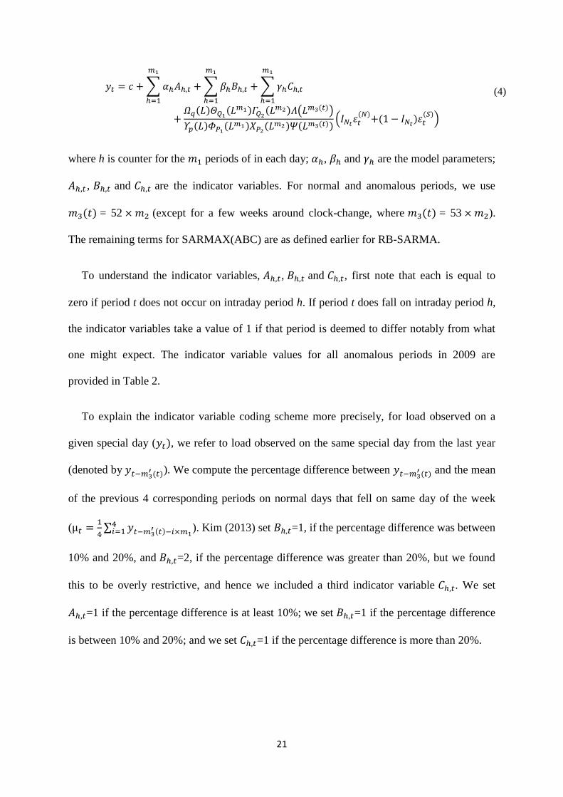
Figure 7— MAPE across only special days for two sophisticated benchmark methods (RB-

HWT and RB-ANN), original version and rule-based adaptation of the SARMA method

(SARMA and RB-SARMA), and SARMAX(ABC).

In Figure 7, we present the MAPE across special days for the best performing methods

from Table 3, across all horizons. Specifically, we plot MAPEs for the SARMA-based

method and the more sophisticated benchmarks. The figure emphasises what we saw in Table

3; most accurate method is RB-SARMA. It comfortably outperforms both the original

SARMA method and the SARMAX(ABC) approach. The SARMAX(ABC) method was only

marginally more accurate than SARMA, which makes no attempt to model the special days.

Furthermore, both RB-HWT and RB-ANN performed better than SARMAX(ABC).

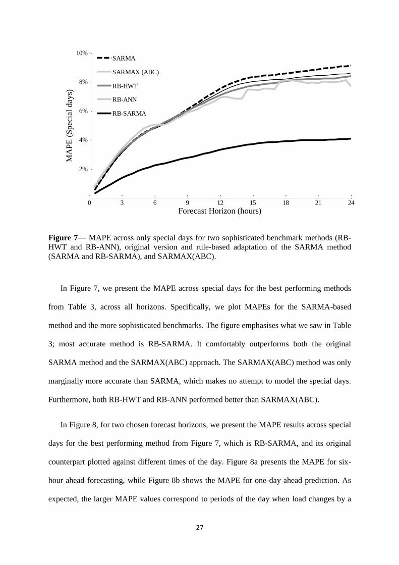
In Figure 8, for two chosen forecast horizons, we present the MAPE results across special

days for the best performing method from Figure 7, which is RB-SARMA, and its original

counterpart plotted against different times of the day. Figure 8a presents the MAPE for six-

hour ahead forecasting, while Figure 8b shows the MAPE for one-day ahead prediction. As

expected, the larger MAPE values correspond to periods of the day when load changes by a

0 3 6 9 12 15 18 21 24

2%

4%

6%

8%

10%

Forecast Horizon (hours)

MA

PE

(S

pecia

l days)

SARMA

SARMAX (ABC)

RB-HWT

RB-ANN

RB-SARMA

28

relatively large amount. For both forecast horizons considered in Figure 8, the accuracy of the

two methods are noticeably different, especially during early morning hours (around 8 am),

when the RB-SARMA method is superior.

Figure 8— MAPE across only special days for SARMA and RB-SARMA, plotted against

different times of the day, with forecast horizon equal to: a) six-hour, and b) one-day.

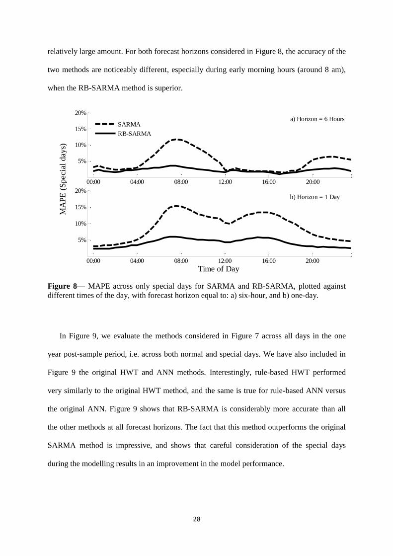
In Figure 9, we evaluate the methods considered in Figure 7 across all days in the one

year post-sample period, i.e. across both normal and special days. We have also included in

Figure 9 the original HWT and ANN methods. Interestingly, rule-based HWT performed

very similarly to the original HWT method, and the same is true for rule-based ANN versus

the original ANN. Figure 9 shows that RB-SARMA is considerably more accurate than all

the other methods at all forecast horizons. The fact that this method outperforms the original

SARMA method is impressive, and shows that careful consideration of the special days

during the modelling results in an improvement in the model performance.

00:00 04:00 08:00 12:00 16:00 20:00

5%

10%

15%

20%

SARMA

RB-SARMA

00:00 04:00 08:00 12:00 16:00 20:00

5%

10%

15%

20%

Time of Day

MA

PE

(S

pecia

l days)

a) Horizon = 6 Hours

b) Horizon = 1 Day

29

Figure 9— MAPE across all days for the original and rule-based adaptations of the SARMA,

HWT exponential smoothing, and the ANN method, along with SARMAX(ABC).

Figure 10— MAPE for each individual special day using the RB-SARMA method, plotted

for forecast horizon corresponding to one-day (numerical MAPE values for each special day

are reported above its corresponding error bar).

0 3 6 9 12 15 18 21 24

0.5%

1%

1.5%

2%

2.5%

3%

Forecast Horizon (hours)

MA

PE

(A

ll d

ays)

ANN

RB-ANN

HWT

RB-HWT

SARMA

SARMAX(ABC)

RB-SARMA

2.5%

5%

7.5%

10%

MA

PE

Day

aft

er N

ew Y

ear'

s

Eas

ter

Mo

nd

ay

Lab

or

Day

WW

II V

icto

ry D

ay

Asc

ensi

on

Day

Day

aft

er A

scen

sio

n

Wh

it M

on

day

Day

bef

ore

Bas

till

e

Bas

till

e D

ay

Th

e A

ssu

mp

tio

n

All

Sai

nts

Day

Rem

emb

ran

ce D

ay

Ch

rist

mas

Wee

k

Ch

rist

mas

Wee

k

Ch

rist

mas

Wee

k

Ch

rist

mas

Wee

k

Ch

rist

mas

Day

Bo

xin

g D

ay

Ch

rist

mas

Wee

k

Ch

rist

mas

Wee

k

Ch

rist

mas

Wee

k

Ch

rist

mas

Wee

k

New

Yea

rs E

ve

4.5

%

5.5

%

8.7

%

4.2

%

3.8

%

1.9

%

1.9

%

4.3

%

4.1

%

4.9

%

1.5

%

2.2

%

1.9

%

3.7

%

2.8

%

5.0

%

2.2

%

6.5

%

5.5

%

5.1

%

2.5

%

5.4

%

5.6

%

Horizon = 1 Day

30

In Figure 10, we plot the MAPE for one-day ahead forecasting from the RB-SARMA

method for the individual special days in 2009. The plot shows only 23 of the 24 special days

in 2009, because we were not able to produce one-day ahead predictions for each hour on

New Year’s Day 2009, as we had used observations up to, and including, New Year’s Eve

2008 in our estimation sample.

7.2. Density Forecasting

In order to evaluate the density forecast performance, we use the Continuous Ranked

Probability Score (CRPS) (see, for example, Gneiting et al., 2007), as it takes into account

both calibration and sharpness in the evaluation of the density forecasts. We generated

density forecasts using SARMA and RB-SARMA using Monte Carlo simulation with 1000

iterations. Note that as opposed to SARMA, which uses one model error for all days, RB-

SARMA uses different variances for model errors for normal and special days. To evaluate

density forecast accuracy, in Figure 11, we present the CRPS values across special days and

all days for SARMA and RB-SARMA. Note that lower CRPS values are better. It is evident

from Figure 11, that RB-SARMA is considerably more accurate than SARMA, across both

special days and all days, for all lead times. The model rankings based on the CRPS are

consistent with the earlier rankings obtained using the MAPE.

31

Figure 11— CRPS for SARMA and RB-SARMA, plotted across different horizons for only:

a) Special days, and b) All days.

8. Summary and Concluding Remarks

In this paper, we presented a case study on load forecasting for France, with emphasis on

forecasting load on special days using a rule-based SARMA method, developed by Arora and

Taylor (2013) for British load data. In comparison with that study, modelling anomalous load

for France is more challenging, due to the relatively large number of different types of special

days in France. This extra complexity in the data necessitated our development of a new rule,

formulated such that each special day is treated as having a unique profile that allows for

greater flexibility during the modelling. A further methodological development in this paper

is our adaptation of a SARMA method recently proposed in this journal for anomalous load

(see Kim, 2013).

Overall, we found that the rule-based SARMA method generated the most accurate

forecasts for special days. For these days, the MAPE obtained using rule-based SARMA was

about one-third of the MAPE for the simple benchmark methods, and about a half of the

0 3 6 9 12 15 18 21 24

1000

2000

3000

4000

5000

SARMA

RB-SARMA

0 3 6 9 12 15 18 21 240

500

1000

1500

Forecast Horizon (hours)

CR

PS

b) All days

a) Special days

32

MAPE of the original SARMA method, which is not rule-based and which makes no attempt

to model special days. Moreover, while evaluating the probability density forecast accuracy

using the CRPS, the performance of rule-based SARMA was noticeably superior to SARMA.

Encouragingly, the rule-based SARMA method was considerably more accurate than rule-

based HWT and rule-based ANN methods. Although the inclusion of additional indicator

variable in the formulation of Kim’s SARMAX method led to substantial improvements in its

accuracy, it was notably outperformed by the rule-based SARMA method. One of the most

encouraging findings in our study was that, in comparison with the original SARMA model,

that treats special days no differently from normal days, the use of rule-based SARMA led to

a noticeable improvement in accuracy when evaluated over special days.

Crucially, as opposed to some of the previous approaches, which employ different models

for normal and special days, the rule-based methods investigated in this study model load for

all days in a unified and coherent framework. This modelling approach makes the task of

generating multistep density forecasts relatively straightforward. Moreover, the proposed

methodology can potentially be adapted for other applications. Some examples where this

approach could be useful includes forecasting call centre arrivals, hospital admissions, water

usage, and transportation counts, as the corresponding time series exhibit seasonality and

anomalous conditions, which pose significant modelling challenges. In this paper, we have

considered only univariate methods. With a view to producing forecasts for longer lead times,

an interesting and potentially useful line of future work would be to consider how the rule-

based adaptations presented in this paper could be incorporated in a weather-based model.

Acknowledgement

We are very grateful to the International Institute of Forecasters (IIF) and SAS for funding

this research. We would also like to thank the Editor and two anonymous referees for their

useful comments and suggestions.

33

References

Adyaa, M., Collopy, F., Armstrong, J.S. and Kennedy, M. (2000). An application of rule-

based forecasting to a situation lacking domain knowledge, International Journal of

Forecasting, 16, 477–484.

Armstrong, J.S. (2001). Principles of forecasting: A handbook for researchers and

practitioners. Kluwer Academic Publishers, Boston.

Armstrong, J.S. (2006). Findings from evidence-based forecasting: Methods for reducing

forecast error, International Journal of Forecasting, 22, 583–598.

Arora, S. and Taylor, J.W. (2013). Short-term forecasting of anomalous load using rule-based

triple seasonal methods, IEEE Transactions on Power Systems, 28, 3235–3242.

Arora, S. and Taylor, J.W. (2016). Forecasting electricity smart meter data using conditional

kernel density estimation, Omega, 59, 47–59.

Atiya, A.F., El-Shoura, S.M., Shaheen, S.I. and El-Sherif, M.S. (1999). A comparison

between neural-network forecasting techniques–case study: river flow forecasting, IEEE

Transactions on Neural Networks, 10, 402–409.

Barrow, D. and Kourentzes, N. (2016). The impact of special days in call arrivals forecasting:

A neural network approach to modelling special days, European Journal of Operational

Research, in press.

Box, G.E.P. and Jenkins, G.M. (1970). Time series analysis, forecasting and control, San

Francisco: Holden–Day.

Bunn, D.W. (1982). Short-term forecasting: A review of procedures in the electricity supply

industry, The Journal of the Operational Research Society, 33, 533–545.

Bunn, D.W. (2000). Forecasting loads and prices in competitive power markets, Proceedings

of the IEEE, 88, 163–169.

Cancelo, J.R., Espasa, A. and Grafe, R. (2008). Forecasting the electricity load from one day

to one week ahead for the Spanish system operator, International Journal of Forecasting,

24, 588–602.

Cho, H., Goude, Y., Brossat, X. and Yao, Q. (2013). Modeling and forecasting daily

electricity load curves: a hybrid approach, Journal of the American Statistical

Association, 108, 7–21.

Collopy, F. and Armstrong, J.S. (1992). Rule-based forecasting: development and validation

of expert systems approach to combining time series extrapolations, Management

Science, 38, 1394–1414.

Cottet, R. and Smith., M. (2003). Bayesian modelling and forecasting of intraday electricity

load, Journal of the American Statistical Association, 98, 839–849.

De Livera, A.M., Hyndman, R.J. and Snyder, R.D. (2011). Forecasting time series with

complex seasonal patterns using exponential smoothing, Journal of the American

Statistical Association, 106, 1513–1527.

34

Dordonnat, V., Koopman, S.J., Ooms, M., Dessertaine, A. and Collet, J. (2008). An hourly

periodic state space model for modelling French national electricity load, International

Journal of Forecasting, 24, 566–587.

Gneiting, T., Balabdaoui, F. and Raftery, A.E. (2007). Probabilistic forecasts, calibration and

sharpness, Journal of the Royal Statistical Society, 69, 243–268.

Gould, P.G., Koehler, A.B., Ord, J.K., Snyder, R.D., Hyndman, R.J. and Vahid-Araghi, F.

(2008). Forecasting time series with multiple seasonal patterns, European Journal of

Operational Research, 191, 207–222.

Hippert, H.S., Bunn, D.W. and Souza, R.C. (2005). Large scale neural networks for

electricity load forecasting: Are they overfitted?, International Journal of Forecasting,

21, 425–434.

Hyde, O. and Hodnett, P.F. (1993). Rule-based procedures in short-term electricity load

forecasting, IMA Journal of Mathematics Applied in Business and Industry, 5, 131–141.

Hyde, O. and Hodnett, P.F. (1997). An adaptable automated procedure for short-term

electricity load forecasting, IEEE Transactions on Power Systems, 12, 84–94.

Kim, K-H., Youn, H-S. and Kang, Y-C. (2000). Short-term load forecasting for special days

in anomalous load conditions using neural networks and fuzzy inference method, IEEE

Transactions on Power Systems, 15, 559–565.

Kim, M.S. (2013). Modeling special-day effects for forecasting intraday electricity demand,

European Journal of Operational Research, 230, 170–180.

Lagarias, J. C., Reeds, J. A., Wright, M. H. and Wright, P. E (1998). Convergence properties

of the Nelder-Mead simplex method in low dimensions. SIAM Journal of Optimization, 9,

112–147.

Pardo, A., Meneu, V. and Valor, E. (2002). Temperature and seasonality influences on

Spanish electricity load, Energy Economics, 24, 55–70.

Rahman, S. and Bhatnagar, R. (1988). An expert system based algorithm for short term load

forecast, IEEE Transactions on Power Systems, 3, 392–399.

Ramanathan, R., Engle, R., Granger, C.W.J., Vahid-Araghi, F. and Brace, C. (1997). Short-

run forecasts of electricity load and peaks, International Journal of Forecasting, 13, 161–

174.

Smith, M. (2000). Modeling and short-term forecasting of New South Wales electricity

system load, Journal of Business Economics and Statistics, 18, 465–478.

Soares, L.J. and Medeiros, M.C. (2008). Modelling and forecasting short-term electricity

load: A comparison of methods with an application to Brazilian data, International

Journal of Forecasting, 24, 630–644.

Taylor, J.W. (2008). An evaluation of methods for very short-term load forecasting using

minute-by-minute British data, International Journal of Forecasting, 24, 645–658.

Taylor, J.W. (2010). Triple seasonal methods for electricity demand forecasting, European

Journal of Operations Research, 204, 139–152.

35

Weron, R. (2006). Modelling and Forecasting Electric Loads and Prices. Chichester, Wiley.