Variational inference for

Dirichlet process mixtures

David M. Blei

School of Computer ScienceCarnegie-Mellon University

blei@cs.cmu.edu

Michael I. Jordan

Computer Science Division and Department of StatisticsUniversity of California, Berkeleyjordan@stat.berkeley.edu

October 5, 2004

Abstract

Dirichlet process (DP) mixture models are the cornerstone of nonpara-metric Bayesian statistics, and the development of Monte-Carlo Markov chain(MCMC) sampling methods for DP mixtures has enabled their applications toa variety of practical data analysis problems. However, MCMC sampling canbe prohibitively slow, and it is important to explore alternatives. One classof alternatives is provided by variational methods, a class of deterministic al-gorithms that convert inference problems into optimization problems (Opperand Saad, 2001; Wainwright and Jordan, 2003). Thus far, variational meth-ods have mainly been explored in the parametric setting, in particular withinthe formalism of the exponential family (Attias, 2000; Ghahramani and Beal,2001; Blei et al., 2003). In this paper, we present a variational inference algo-rithm for DP mixtures. We present experiments that compare the algorithmto Gibbs sampling algorithms for DP mixtures of Gaussians and present anapplication to a large-scale image analysis problem.

1

1 Introduction

The methodology of Monte Carlo Markov chain (MCMC) sampling has energizedBayesian statistics during the past decade, providing a systematic approach to thecomputation of likelihoods and posterior distributions, and permitting the deploy-ment of Bayesian methods in a rapidly growing number of applied problems. How-ever, while an unquestioned success story, MCMC is not an unqualified successstory—MCMC methods can be slow to converge and their convergence can be diffi-cult to diagnose. While further research on sampling is needed, it is also importantto explore alternatives, particularly in the context of large-scale problems.

One such class of alternatives is provided by variational inference methods (Ghahra-mani and Beal, 2001; Jordan et al., 1999; Opper and Saad, 2001; Wainwright andJordan, 2003; Wiegerinck, 2000). Like MCMC, variational inference methods havetheir roots in statistical physics, and, in contradistinction to MCMC methods, theyare deterministic. The basic idea of variational inference is to formulate the compu-tation of a marginal or conditional probability in terms of an optimization problem.This (generally intractable) problem is then “relaxed,” yielding a simplified opti-mization problem that depends on a number of free parameters, known as variationalparameters. Solving for the variational parameters gives an approximation to themarginal or conditional probabilities of interest.

Variational inference methods have been developed principally in the contextof the exponential family, where the convexity properties of the natural parame-ter space and the cumulant generating function yield an elegant general variationalformalism (Wainwright and Jordan, 2003). For example, variational methods havebeen developed for parametric hierarchical Bayesian models based on general expo-nential family specifications (Ghahramani and Beal, 2001). MCMC methods haveseen much wider application. In particular, the development of MCMC algorithmsfor nonparametric models such as the Dirichlet process has led to increased interestin nonparametric Bayesian methods. In the current paper, we aim to close this gapand indicate how variational methods can be used in the Dirichlet process setting.

The Dirichlet process (DP), introduced in Ferguson (1973), is parameterized by abase measure G0 and positive scaling parameter α. Writing G | {G0, α} ∼ DP(G0, α)for a draw from the Dirichlet process, suppose that {η1, . . . , ηN} are subsequentlydrawn independently from G: ηn |G ∼ G. Marginalizing out the random measure G,the joint distribution of {η1, . . . , ηN} turns out to follow a Polya urn scheme (Black-well and MacQueen, 1973). Thus, positive probability is assigned to configurationsin which different ηn take on identical values, and the underlying random measureG is discrete with probability one. This is seen most directly in the stick-breakingrepresentation of the DP, in which G is represented explicitly as an infinite sum of

2

atomic measures (Sethuraman, 1994).The Dirichlet process mixture model (Antoniak, 1974) adds a level to the hierar-

chy, treating ηn as the parameter of the distribution of the nth observation. Giventhe discreteness of G, the DP mixture has an interpretation as a mixture model withan unbounded number of mixture components.

Our goal will be to compute the predictive density:

p(x |x1, . . . , xN ) =

∫

p(x | η)p(η |x1, . . . , xN)dη, (1)

under the DP mixture, given a sample {x1, . . . , xN}. As in many hierarchical Bayesianmodels, the posterior distribution p(η |x1, . . . , xN) is complicated and difficult tocharacterize in a closed form in the DP mixture setting. MCMC provides one classof approximations for this posterior and the predictive density (Escobar and West,1995; Neal, 2000).

In this paper, we present a variational inference algorithm for DP mixtures basedon the stick-breaking representation of the underlying DP. The algorithm involvestwo probability distributions—the posterior distribution p and a variational distribu-tion q. The latter is endowed with free variational parameters, and the algorithmicproblem is to adjust these parameters so that q approximates p. We also use a stick-breaking representation for q, but in this case we truncate the representation to yielda finite-dimensional representation. While in principle we could also truncate p, turn-ing the model into a finite-dimensional model, it is important to emphasize at theoutset that this is not our approach—we only truncate the variational distributionand approximate the posterior of an infinite-dimensional model.

The paper is organized as follows. In Section 2 we provide basic background onDP mixture models, focusing on the case of exponential family mixtures. Section 3overviews MCMC algorithms for the DP mixture, discussing algorithms based bothon the Polya urn representation and the stick-breaking representation. In Section 4we present a variational inference algorithm for DP mixtures. Section 5 presents theresults of experimental comparisons and Section 7 presents our conclusions.

2 Dirichlet process mixture models

Let η be a continuous random variable, let G0 be a non-atomic probability distri-bution for η, and let α be a positive, real-valued scalar. A random measure Gis distributed according to a Dirichlet process (DP) (Ferguson, 1973), with scalingparameter α and base measure G0, if for all natural numbers k and k-partitions

3

{B1, . . . , Bk}:

(G(η ∈ B1), G(η ∈ B2), . . . , G(η ∈ Bk)) ∼ Dir(αG0(B1), αG0(B2), . . . , αG0(Bk)).

Integrating out G, the joint distribution of the collection of variables {η1, . . . , ηn}exhibits a clustering effect; conditioned on n−1 draws, the nth value is, with positiveprobability, exactly equal to one of those draws:

p(η | η1, . . . , ηn−1) ∝ αp(η |G0) +n−1∑

i=1

δηi(η). (2)

Thus, {η1, . . . , ηn−1} are randomly partitioned according to which variables are equalto the same value, with the distribution of the partition obtained from a Polya urnscheme (Blackwell and MacQueen, 1973). Let {η∗1, . . . , η

∗|c|} denote the distinct values

of {η1, . . . , ηn−1}, let c = {c1, . . . , cn−1} denote the partition such that ηi = η∗cn, and

let |c| denote the number of groups in that partition. The distribution of ηn followsthe urn distribution:

ηn =

{

η∗i with prob |c|in−1+α

η, η ∼ G0 with prob αn−1+α

,(3)

where |c|i is the number of times the value η∗i occurs in {η1, . . . , ηn−1}.In the Dirichlet process mixture model, the DP is used as a nonparametric prior

in a hierarchical Bayesian model (Antoniak, 1974):

G | {α,G0} ∼ DP(α,G0)

ηn |G ∼ G

Xn | ηn ∼ p(xn | ηn).

Data generated from this model can be partitioned according to those values drawnfrom the same parameter. Thus, the DP mixture has a natural interpretation asa flexible mixture model in which the number of components (i.e., the number ofgroups in the partition) is random and grows as new data are observed.

The urn scheme in Equation (3) provides an implicit definition of the DP. Sethu-raman (1994) provides an explicit definition via a stick-breaking construction of G.Consider two infinite collections of independent random variables, Vi ∼ Beta(1, α)

4

and η∗i ∼ G0, for i = {1, 2, . . .}. We can write G as:

θi = Vi

i−1∏

j=1

(1− Vj) (4)

G(η) =∞∑

i=1

θiδη∗i(η). (5)

Thus the support of G consists of a countably infinite set of atoms, drawn iid from G0.The mixing proportions θi are given by successively breaking a unit length “stick”into an infinite number of pieces. The size of each successive piece, proportional tothe rest of the stick, is given by an independent draw from a Beta(1, α) distribution.

In the DP mixture, the vector θ comprises the infinite vector of mixing proportionsand {η∗1, η

∗2, . . .} are the infinite number of mixture components. Let Zn denote the

mixture component with which xn is associated.1 The data can thus be described asarising from the following process:

1. Draw Vi |α ∼ Beta(1, α), i = {1, 2, . . .}

2. Draw η∗i |G0 ∼ G0, i = {1, 2, . . .}

3. For each data point n:

(a) Draw Zn | {v1, v2, . . .} ∼ Mult(θ).

(b) Draw Xn | zn ∼ p(xn | η∗zn

).

2.1 Exponential family mixtures

In this paper, we restrict ourselves to DP mixtures for which the observable data aredrawn from an exponential family distribution, and where the base measure for theDP is the corresponding conjugate prior.

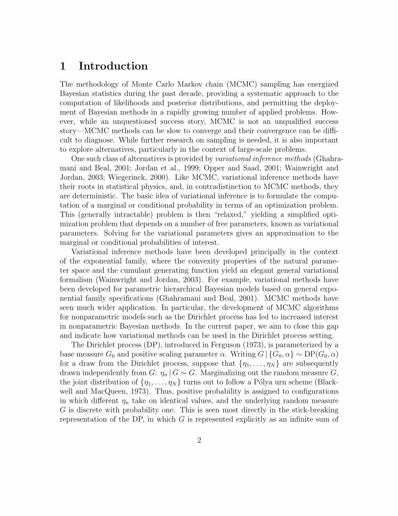
A DP mixture using the stick-breaking construction is illustrated as a graphicalmodel in Figure 1. The distributions of Vk and Zn are as described above. Thedistribution of Xn conditional on Zn and {η∗1, η

∗2, . . .} is:

p(xn | zn, η∗1, η

∗2, . . .) =

∞∏

i=1

(

h(xn) exp{η∗iT xn − a(η∗i )}

)zin ,

1We represent multinomial random vectors as indicator vectors consisting of a single componentequal to one and the remaining components equal to zero.

5

λ

α

N 8

Z

X

V

η*

n

n

k

k

Figure 1: Graphical model representation of an exponential family DP mixture.Nodes denote random variables, edges denote possible dependence, and plates denotereplication.

where a(η∗i ) is the appropriate cumulant generating function and we assume forsimplicity that x is the sufficient statistic for the canonical parameter η.

The vector of sufficient statistics of the corresponding conjugate family is (η∗T ,−a(η∗))T .The base measure is thus:

p(η∗ |λ) = h(η∗) exp{λT1 η∗ + λ2(−a(η∗))− a(λ)},

where we decompose the hyperparameter λ such that λ1 contains the first dim(η∗)components and λ2 is a scalar.

2.2 The truncated Dirichlet process

Ishwaran and James (2001) have discussed the truncated Dirichlet process (TDP), inwhich VK−1 is set equal to one for some fixed value K. This yields θi = 0 for i ≥ K,and thus converts the infinite sum in Equation (4) into a finite sum. Ishwaran andJames (2001) show that a TDP closely approximates a true Dirichlet process whenthe truncation level K is chosen large enough relative to the number of data points.Thus, they can justify substituting a TDP mixture model for a full DP mixturemodel.

3 MCMC for DP mixtures

The posterior distribution under both the DP and TDP mixture models cannot becomputed efficiently in any direct way. It must be approximated, and Markov chain

6

Monte Carlo (MCMC) methods are the method of choice for approximating theseposteriors (Escobar and West, 1995; Neal, 2000; Ishwaran and James, 2001).

As in the parametric setting, the idea behind MCMC for approximate posteriorinference in the DP mixture is to construct a Markov chain for which the stationarydistribution is the posterior of interest. One collects samples from the sample pathof this Markov chain to construct an estimate of the posterior. Such an estimatecan then be used to compute an approximation of the predictive distribution (seeEquation 1).

The simplest MCMC algorithm is the Gibbs sampler, in which the Markov chainis defined by iteratively sampling each latent variable conditional on the data and themost recently sampled values of the other latent variables. This yields a chain withthe desired stationary distribution (Geman and Geman, 1984; Gelfand and Smith,1990; Neal, 1993). Below, we review the Gibbs sampling algorithms for DP and TDPmixtures.

3.1 Collapsed Gibbs sampling

In the collapsed Gibbs sampler for a DP mixture with conjugate base measure (Esco-bar and West, 1995), we integrate out the random measure G and distinct parametervalues {η∗1, . . . , η

∗|c|}. The Markov chain is thus defined only on the latent partition

of the data, c = {c1, . . . , cN}.Denote the data by x = {x1, x2, . . . , xN}. For n ∈ {1, . . . , N}, the algorithm

iteratively samples each group assignment Cn, conditional on the partition of therest of the data c−n. Note that Cn can be assigned to one of |c−n|+ 1 values: eitherthe nth data point is in a group with other data points, or in a group by itself.

By exchangeability, Cn is drawn from the following multinomial distribution:

p(ckn = 1 |x, c−n, λ, α) ∝ p(xn |x−n, c−n, c

kn = 1, λ)p(ck

n = 1 | c−n, α). (6)

The first term is a ratio of normalizing constants of the posterior distribution of thekth parameter, one including and one excluding the nth data point:

p(xn |x−n, c−n, ckn = 1, λ) =

exp{

a(λ1 +∑

m6=n ckmXm + Xn, λ2 +

∑

m6=n ckm + 1)

}

exp{

a(λ1 +∑

m ckmXm, λ2 +

∑

m6=n ckm)} .

(7)The second term is given by the Polya urn scheme:

p(ckn = 1 | c−n) ∝

{

|c−n|k if k is an existing group in the partitionα if k is a new group in the partition,

(8)

7

where |c−n|k denotes the number of data in the kth group of the partition.Once this chain has reached its stationary distribution, we collect B samples

{c1, . . . , cB} to approximate the posterior. The approximate predictive distributionis an average of the predictive distributions for each of the collected samples:

p(xN+1 |x1, . . . , xN , α, λ) =1

B

B∑

b=1

p(xN+1 | cb,x, α, λ).

For a particular sample, that distribution is:

p(xN+1 | c,x, α, λ) =

|c|+1∑

k=1

p(ckN+1 = 1 | c)p(x | c,x, ck

N+1 = 1).

When G0 is not conjugate, the integral in Equation (7) does not have a simpleclosed form. Effective algorithms for handling this case are given in Neal (2000).

3.2 Blocked Gibbs sampling

In the collapsed Gibbs sampler, the distribution of each partition group variable Cn

depends on the most recently sampled values of the other variables. Thus, thesevariables must be updated one at a time, which could potentially slow down thealgorithm when compared to a blocking strategy. To this end, Ishwaran and James(2001) developed an inference algorithm based on the TDP described in Section 2.By explicitly sampling an approximation of G, this model allows for a blocked Gibbssampler, in which collections of variables can be updated simultaneously.

The state of the Markov chain consists of the beta variables V = {V1, . . . , VK−1},the component parameters η

∗ = {η∗1, . . . , η∗K}, and the component assignment vari-

ables Z = {Z1, . . . , ZN}. The blocked Gibbs sampler iterates between the followingthree steps:

1. For n ∈ {1, . . . , N}, independently sample Zn from:

p(zkn = 1 |v,η∗,x) = θkp(xn | η

∗k),

where θk is the function of v given in Equation (4).

2. For k ∈ {1, . . . , K}, independently sample Vk from Beta(γk,1, γk,2), where:

γk,1 = 1 +∑N

n=1 zkn

γk,2 = α +∑K

i=k+1

∑N

n=1 zin.

8

This step follows from the conjugacy between the multinomial data z and thetruncated stick-breaking construction, which is a generalized Dirichlet distri-bution (Connor and Mosimann, 1969).

3. For k ∈ {1, . . . , K}, independently sample η∗k from p(η∗k | τk). This distributionis in the same family as the base measure, with parameters:

τk,1 = λ1 +∑

i6=n zki xi

τk,2 = λ2 +∑

i6=n zki .

(9)

After the chain has reached its stationary distribution, we collect B samplesand construct an approximate predictive distribution. Again, this distribution isan average of the predictive distributions for each of the collected samples. Thepredictive distribution for a particular sample is:

p(xN+1 | z,x, α, λ) =K∑

k=1

E [θi | γ1, . . . , γk] p(xN+1 | τk), (10)

where E [θi | γ1, . . . , γk] is the expectation of the product of independent beta variablesgiven in Equation (4). This distribution only depends on z; the other variables areneeded in the Gibbs sampling procedure, but can be integrated out here.

The TDP sampler readily handles non-conjugacy of G0, provided that there is amethod of sampling η∗i from its posterior.

3.3 Placing a prior on the scaling parameter

A common extension to the DP mixture model involves placing a prior on the scal-ing parameter α, which determines how quickly the number of components growswith the data. For the urn-based samplers, Escobar and West (1995) place aGamma(s1, s2) prior on α and implement the corresponding Gibbs updates withauxiliary variable methods.

In the TDP mixture, the gamma distribution is computationally convenient be-cause it is conjugate to Beta(1, α) (see Appendix A). The Gibbs updates for α arethus:

α | {v, s1, s2} ∼ Gamma

(

s1 + K − 1, s2 −K−1∑

i=1

log(1− vi)

)

. (11)

9

4 Variational inference for the DP mixture

Variational inference provides an alternative, deterministic methodology for approx-imating likelihoods and posteriors in an intractable probabilistic model (Wainwrightand Jordan, 2003). We first review the basic idea in the context of the exponentialfamily of distributions, and then turn to its application to DP mixture models.

Consider the exponential family indexed by the natural parameter θ:

p(z | θ) = exp{θT t(z)− a(θ)}h(z),

where t(z) is the vector of sufficient statistics. The cumulant generating functiona(θ), also known as the log partition function, is defined as follows:

a(θ) = log

∫

exp{θT t(z)}h(z)dz.

As discussed by Wainwright and Jordan (2003), this quantity can also be expressedvariationally as:

a(θ) = supµ∈M

{θT µ− a∗(µ)}, (12)

where a∗(µ) is the Fenchel-Legendre conjugate of a(θ) (Rockafellar, 1970), and M is

the set of realizable expected sufficient statistics : M = {µ : µ =∫

t(z)p(z)h(z)dz, for some p}.There is a one-to-one mapping between parameters θ and the interior of M (Brown,1986). Accordingly, the interior of M is often referred to as the set of mean param-eters.

Let θ(µ) be a natural parameter corresponding to the mean parameter µ ∈ M;thus Eθ [t(Z)] = µ. Let q(z | θ(µ)) denote the corresponding density. Given µ ∈ M,a short calculation shows that a∗(µ) is the negative entropy of q:

a∗(µ) = Eθ(µ) [log q(Z | θ(µ))] . (13)

Given its definition as a Fenchel conjugate, the negative entropy is convex.In many models of interest, a(θ) is not feasible to compute because of the com-

plexity of M or the lack of any explicit form for a∗(µ). However, we can bound a(θ)using Equation (12):

a(θ) ≥ µT θ − a∗(µ), (14)

for any mean parameter µ ∈ M. Moreover, the tightness of the bound is measuredby a Kullback-Leibler divergence expressed in terms of a mixed parameterization:

D(q(z | θ(µ)) || p(z | θ)) = Eθ(µ) [log q(z | θ(µ))− log p(z | θ)]

= θ(µ)T µ− a(θ(µ))− θT µ + a(θ)

= a(θ)− θT µ + a∗(θ(µ)). (15)

10

Mean-field variational methods are a special class of variational methods that arebased on maximizing the bound in Equation (14) with respect to a subset Mtract

of the space M of realizable mean parameters. In particular, Mtract is chosen sothat a∗(θ(µ)) can be evaluated tractably and so that the maximization over Mtract

can be performed tractably. Equivalently, given the result in Equation (15), mean-field variational methods minimize the KL divergence D(q(z | θ(µ)) || p(z | θ)) withrespect to its first argument.

If the distribution of interest is a posterior, then a(θ) is the log likelihood. Con-sider in particular a latent variable probabilistic model with hyperparameters θ,observed variables x = {x1, . . . , xN}, and latent variables z = {z1, . . . , zM}. Theposterior can be written as:

p(z |x, θ) = exp{log p(z,x | θ)− log p(x | θ)}, (16)

and the bound in Equation (14) applies directly. We have:

log p(x | θ) ≥ Eq [log p(x,Z | θ)]− Eq [log q(Z)] . (17)

This equation holds for any q via Jensen’s inequality, but, as our analysis has shown,it is useful specifically for q of the form q(z | θ(µ)) for µ ∈Mtract.

A straightforward way to construct tractable subfamilies of exponential fam-ily distributions is to consider factorized families, in which each factor is an ex-ponential family distribution depending on a so-called variational parameter. In

particular, let us consider distributions of the form q(z |ν) =∏M

i=1 q(zi | νi), where

ν = {ν1, ν2, ..., νM} are variational parameters. Using this class of distributions, wesimplify the likelihood bound using the chain rule:

log p(x | θ) ≥ log p(x | θ)+M∑

m=1

Eq [log p(Zm |x, Z1, . . . , Zm−1, θ)]−M∑

m=1

Eq [log q(Zm | νm)] .

(18)To obtain the best approximation available within the factorized subfamily, we nowwish to optimize this expression with respect to νi.

To optimize with respect to νi, reorder z such that zi is last in the list. Theportion of Equation (18) depending on νi is:

`i = Eq [log p(zi | z−i,x, θ)]− Eq [log q(zi | νi)] . (19)

Given our assumption that the variational distribution q(zi | νi) is in the exponentialfamily, we have:

q(zi | νi) = h(zi) exp{νTi zi − a(νi)},

11

and Equation (19) simplifies as follows:

`i = Eq

[

log p(Zi |Z−i,x, θ)− log h(Zi)− νTi Zi + a(νi)

]

= Eq [log p(Zi |Z−i,x, θ)]− Eq [log h(Zi)]− νTi a′(νi) + a(νi),

because Eq [Zi] = a′(νi). The derivative with respect to νi is:

∂

∂νi

`i =∂

∂νi

(Eq [log p(Zi |Z−i,x, θ)]− Eq [log h(Zi)])− νTi a′′(νi). (20)

Thus the optimal νi satisfies:

νi = [a′′(νi)]−1

(

∂

∂νi

Eq [log p(Zi |Z−i,x, θ)]−∂

∂νi

Eq [log h(Zi)]

)

. (21)

The result in Equation (21) is general. In many applications of mean field meth-ods, a further simplification is achieved. In particular, when the conditional distri-bution p(zi | z−i,x, θ) is an exponential family distribution2, we have:

p(zi | z−i,x, θ) = h(zi) exp{gi(z−i,x, θ)T zi − a(gi(z−i,x, θ))},

where gi(z−i,x, θ) denotes the natural parameter for zi when conditioning on theremaining latent variables and the observations. This yields simplified expressionsfor the expected log probability of Zi and its first derivative:

Eq [log p(Zi |Z−i,x, θ)] = E [log h(Zi)] + Eq [gi(Z−i,x, θ)]T a′(νi)− Eq [a(gi(Z−i,x, θ))]

∂

∂νi

Eq [log p(Zi |Z−i,x, θ)] =∂

∂νi

Eq [log h(Zi)] + Eq [gi(Z−i,x, θ)]T a′′(νi).

Using the first derivative in Equation (21), the maximum is attained at:

νi = Eq [gi(Z−i,x, θ)] . (22)

We define a coordinate ascent algorithm based on Equation (22) by iteratively updat-ing νi for i ∈ {1, . . . , N}. Such an algorithm finds a local maximum of Equation (17)by Proposition 2.7.1 of Bertsekas (1999), under the condition that the right-hand

2Examples in which p(zi | z−i,x, θ) is an exponential family distribution include Kalman filters,hidden Markov models, mixture models, hierarchical Bayesian models with conjugate and mixtureof conjugate priors, and the hierarchical nonparametric Bayesian models which are the focus of thispaper.

12

side of Equation (19) is strictly convex. Further perspectives on algorithms of thiskind can be found in Xing et al. (2003) and Beal (2003).

Notice the interesting relationship of this algorithm to the Gibbs sampler. InGibbs sampling, we iteratively draw the latent variables zi from the distributionp(zi | z−i,x, θ). In mean-field variational inference, we iteratively update the vari-ational parameters of zi to be equal to the expected value of the parameter gi ofthe conditional distribution p(zi | z−i,x, θ), where the expectation is taken under the

variational distribution.3

4.1 Variational inference for DP mixtures

We develop a mean-field variational algorithm for the DP mixture based on the stick-breaking representation of the DP mixture in Figure 1. Using this representation,the bound on the likelihood given in Equation (17) becomes:

log p(x |α, λ) ≥Eq [log p(V |α)] + Eq [log p(η∗ |λ)]

+N∑

n=1

(Eq [log p(Zn |V)] + Eq [log p(xn |Zn)])

− Eq [log q(Z,V,η∗)] .

(23)

The issue that we must face to make use of this bound is that of constructing anapproximation to the distribution of the infinite-dimensional random measure G,expressed in terms of the infinite sets V = {V1, V2, . . .} and η

∗ = {η∗1, η∗2, . . .}. Our

approach is based on using truncated stick-breaking representations for the varia-tional distributions. Thus, we fix a value T and let q(vT = 1) = 1. As in thetruncated Dirichlet process, under the truncated variational distribution, the mix-ture proportions θt are equal to zero for t > T and we can thus ignore the parametersη∗t for t > T .

The factorized distribution that we propose to use as a basis for mean-field vari-ational inference is thus of the following form:

q(v,η∗, z, T ) =T−1∏

t=1

q(vi | γi)T∏

t=1

q(η∗t | τt)N∏

n=1

q(zn |φn), (24)

where γn are the parameters for a beta distribution, τt are natural parameters forthe distributions of η∗t , and φn are parameters for a multinomial distribution.

3This relationship has inspired the software package VIBES (Bishop et al., 2003), which is a

variational version of the popular BUGS package (Gilks et al., 1996).

13

Notice that in the model of Figure 1, the variables V, η∗, and Z are each iden-

tically distributed, whereas, under the variational distribution, there is a differentparameter for each variable. For example, the choice of the mixture component zn forthe nth data point is governed by a multinomial distribution indexed by a variationalparameter φn that depends on n. This reflects the conditional nature of variationalinference.

We emphasize the difference between role that truncation plays in our variationalmethod and the role that it plays in the blocked Gibbs sampler of Ishwaran andJames (2001) (see Section 3.2). The blocked Gibbs sampler estimates the posteriorof a truncated approximation to the DP. In contrast, we use a truncated stick-breaking distribution to approximate the true posterior of a full DP mixture model—the posterior itself is not truncated. The truncation level T is a variational parameterwhich can be freely set; it is not a part of the prior model specification.

4.2 Coordinate-ascent algorithm

We now derive a coordinate-ascent algorithm for optimizing the bound in Equa-tion (23) with respect to the variational parameters. The third term in the bound isthe only term that requires attention, as all of the other terms in the bound involvestandard computations in the exponential family. We rewrite the third term usingindicator random variables:

Eq [log p(Zn |V)] = Eq

[

log(

∏T

i=1(1− Vi)1[Zn>i]V

Zin

i

)]

=∑T

i=1 q(zn > i)E [log(1− Vi)] + q(zn = i)E [log Vi] ,

where:

q(zn = i) = φn,i

q(zn > i) =∑K

j=i+1 φn,j

E [log Vi] = Ψ(γi,1)−Ψ(γi,1 + γi,2)

E [log(1− Vi)] = Ψ(γi,2)−Ψ(γi,1 + γi,2).

(Note that Ψ is the digamma function arising from the derivative of the log normal-ization factor in the beta distribution.)

We now use the general expression in Equation (21) to derive a mean-field coor-dinate ascent algorithm. Computing the derivatives with respect to the variationalparameters, the bound in Equation (23) is optimized via the following set of updates,

14

for t ∈ {1, . . . , T} and n ∈ {1, . . . , N}:

γt,1 = 1 +∑

n φn,t (25)

γt,2 = α +∑

n

∑T

j=t+1 φn,j (26)

τt,1 = λ1 +∑

n φn,txn (27)

τt,2 = λ2 +∑

n φn,t. (28)

φn,t ∝ exp(S), (29)

where:

S = E [log Vt | γt] + E [ηt | τt]T Xn − E [a(ηt) | τt]−

T∑

j=t+1

E [log(1− Vj) | γj] .

Iterating these updates optimizes Equation (23) with respect to the variational pa-rameters defined in Equation (24). That is, we find q(v,η∗, z) which, when pluggedin to the factored expression displayed in Equation (24), yield a distribution that isa mean-field approximation to the true posterior.

Practical applications of variational methods must address initialization of thevariational distribution. While the algorithm yields a bound for any starting valuesof the variational parameters, poor choices of initialization can lead to local maximathat yield poor bounds. We initialize the variational distribution by incrementallyupdating the parameters according to a random permutation of the data points. Ina sense, this is a variational version of sequential importance sampling. We run thealgorithm multiple times and choose the final parameter settings that give the bestbound on the marginal likelihood.

Given a (possibly locally) optimal set of variational parameters, the approximatepredictive distribution is:

p(xN+1 | z,x, α, λ) =T∑

t=1

Eq [θt |γ] Eq [p(xN+1 | τt)] . (30)

This approximation has a form similar to the approximate predictive distributionunder the blocked Gibbs sampler in Equation (10). In the variational case, however,the averaging is done parametrically via the variational distribution rather than bya Monte Carlo integral.

When G0 is not conjugate, a simple coordinate ascent update for τi may not beavailable if p(η∗i | z,x, λ) is not in the exponential family. However, if G0 is a mixtureof conjugate priors, then a simple coordinate ascent algorithm is available.

15

Finally, we extend the variational inference algorithm to posterior updates forthe scaling parameter α with a Gamma(s1, s2) prior. Using the exact posterior of αin Equation (11), the variational posterior Gamma(w1, w2) distribution is:

w1 = s1 + T − 1

w2 = s2 −T−1∑

i=1

Eq [log(1− Vi)]),

and we replace α with its expectation Eq [α |w] = w1/w2 in the updates for γt,2 inEquation (26).

4.3 Discussion

Qualitatively, variational methods offer several potential advantages over Gibbs sam-pling. They are deterministic, and have an optimization criterion given by Equa-tion (23) that can be used to assess convergence. In contrast, assessing convergenceof a Gibbs sampler—namely, determining when the Markov chain has reached itsstationary distribution—is an active field of research. Theoretical bounds on themixing time are of little practical use, and there is no consensus on how to chooseamong the several empirical methods developed for this purpose (Robert and Casella,1999).

Furthermore, in this context, the variational technique provides an explicit esti-mate of the infinite-dimensional parameter G by using the truncated stick-breakingconstruction. The best Gibbs samplers (e.g., the collapsed Gibbs sampler) marginal-ize out G and rely on the Polya urn scheme representation (Neal, 2000). This pre-cludes computation of quantities, such as quantiles, which cannot be expressed asexpectations of G. (See Gelfand and Kottas (2002) for a method which combinesurn-based sampling and TDP-based blocked sampling to compute such quantities.)

But there are several potential disadvantages of variational methods as well. First,variational methods are deterministic optimization procedures that can fall prey tolocal minima. Local minima can be mitigated with restarts, or removed via the in-corporation of additional variational parameters, but these strategies may slow theoverall convergence of the procedure and nullify the advantage over MCMC. Second,any given fixed variational representation yields only an approximation to the pos-terior. There are methods for considering hierarchies of variational representationsthat approach the posterior in the limit, but these methods may again incur seriouscomputational costs. Lacking a theory by which these issues can be evaluated in thegeneral setting of DP mixtures, we turn to experimental evaluation.

16

−40

−20

020

4060

−20 −10 0 10 20

−40

−20

020

4060

initial

−40

−20

020

4060

−20 −10 0 10 20−

40−

200

2040

60

iteration 2

−40

−20

020

4060

−20 −10 0 10 20

−40

−20

020

4060

iteration 5

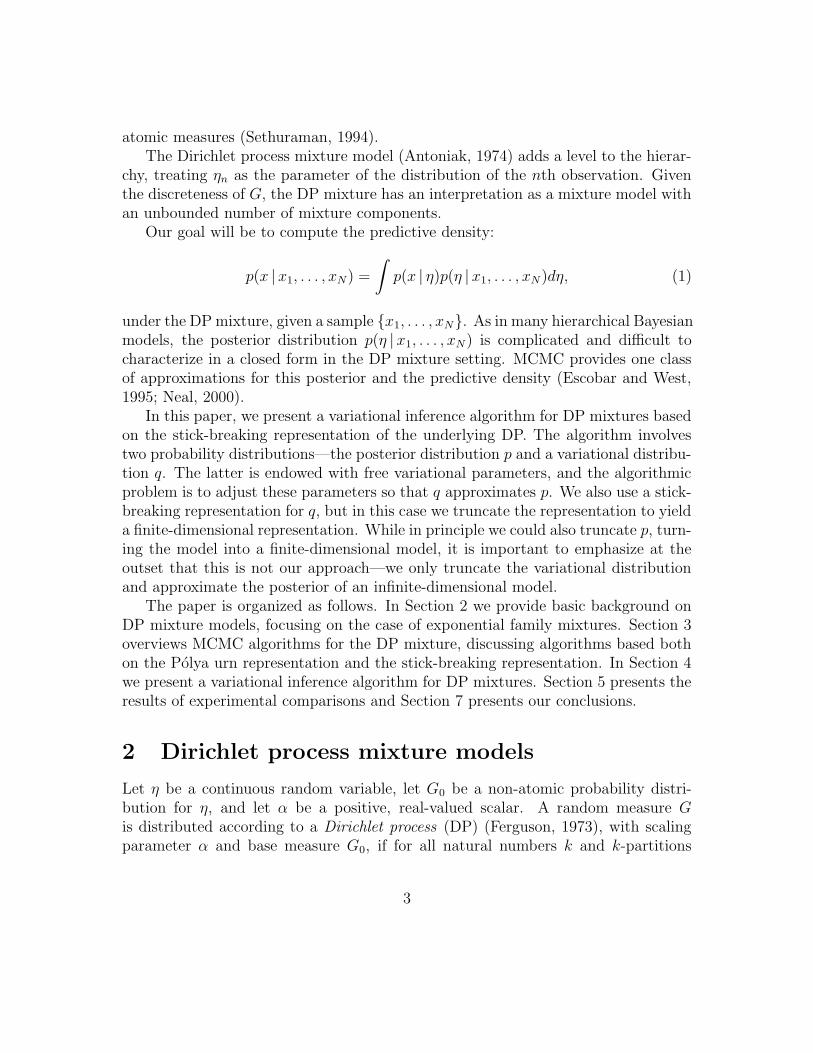
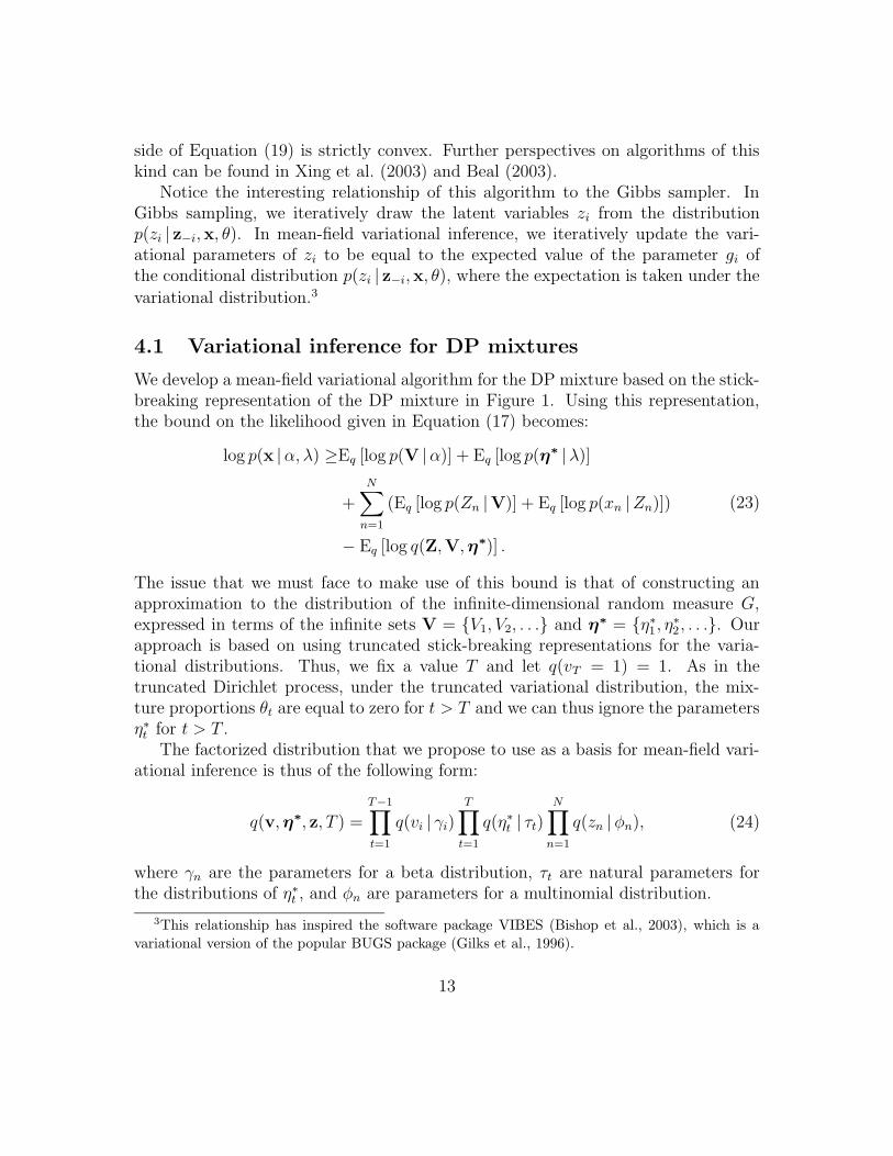
Figure 2: The approximate predictive distribution given by variational inference atdifferent stages of the algorithm. The data are 100 points generated by a GaussianDP mixture model with fixed diagonal covariance.

5 Empirical comparison

We studied the performance of the variational algorithm of Section 4 and the Gibbssamplers of Section 3 in the setting of Gaussian DP mixtures. Thus, likelihood isGaussian with fixed covariance matrix Λ and the Dirichlet process mixes over themean of the Gaussian. The base measure for the DP is Gaussian, with covariancegiven by Λ/λ2, which is conjugate to the likelihood.

Figure 2 provides an illustrative example of the variational inference algorithm ona small problem involving 100 data points sampled from a two-dimensional GaussianDP mixture with diagonal covariance. Each panel in the figure illustrates the dataand the predictive distribution given by the variational inference algorithm, withtruncation level 20. As seen in the first panel, the initialization of the variationalparameters yields a largely flat distribution on the data. After one iteration, thealgorithm has found the modes of the predictive distribution and, after convergence,it has further refined those modes. Even though 20 mixture components are repre-sented in the variational distribution, the fitted approximate posterior only uses fiveof them.

To compare the variational inference algorithm to the Gibbs sampling algorithms,we conducted a systematic set of experiments in which the dimensionality of the datawas varied from 5 to 50. In each case, we generated 100 data from a Gaussian DPmixture model of the chosen dimensionality and generated 100 additional points asheld-out data. In testing on the held-out data, each point is treated as the 101st

17

5 10 20 30 40 50

010

0020

0030

0040

00

Dimension

Tim

e (s

econ

ds)

VarTDPCDP

5 10 20 30 40 50

−12

00−

1000

−80

0−

600

−40

0−

200

Dimension

Hel

d−ou

t log

like

lihoo

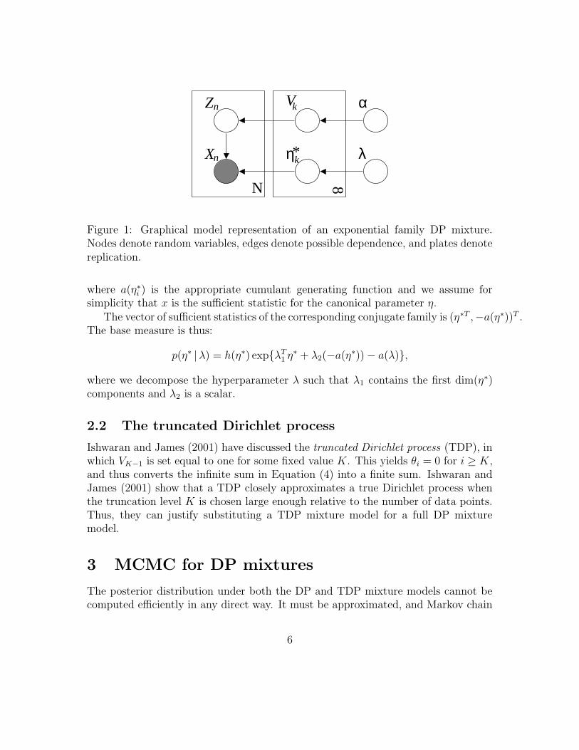
dFigure 3: (Left) Convergence time across ten datasets per dimension for variationalinference, TDP Gibbs sampling, and the collapsed Gibbs sampler (grey bars are stan-dard error). (Right) Average held-out log likelihood for the corresponding predictivedistributions.

data point in the collection.The covariance matrix was given by the autocorrelation matrix for a first-order

autogressive process, chosen so that the components are highly dependent (ρ = 0.9).The base measure was a zero-mean Gaussian with covariance appropriately scaledfor comparison across dimensions. The scaling parameter α was set equal to one.

We ran all algorithms to convergence and measure the computation time.4 Con-vergence was assessed in the following way. For the Gibbs samplers, we assess conver-gence to the stationary distribution with the diagnostic given by Raftery and Lewis(1992), and collect 25 additional samples to estimate the predictive distribution (thesame diagnostic provides an appropriate lag at which to collect uncorrelated sam-ples). The TDP approximation and variational posterior approximation are bothtruncated at 20 components. For the variational inference algorithm we measureconvergence by the relative change in the likelihood bound, stopping the algorithmwhen it is less than 1e−10. Note that there is a certain inevitable arbitrariness inthese choices; in general it is difficult to envisage measures of computation time thatallow stochastic MCMC algorithms and deterministic variational algorithms to be

4All timing computations were made on a Pentium III 1GHZ desktop machine.

18

2 4 6 8 10

−13

50−

1300

−12

50−

1200

−11

50−

1100

Iteration

Hel

d−ou

t log

like

lihoo

d

1e−131e−91e−51e−31e−2

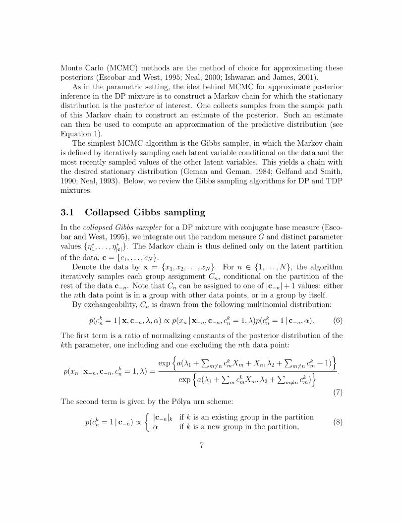
Figure 4: Held-out likelihood as a function of iteration of the variational inferencealgorithm for a 50-dimensional simulated dataset. The relative change in likelihoodbound is labeled at selected iterations.

compared in a standardized way. Nonetheless, we have made what we consider to bereasonable, pragmatic choices. Note in particular that the choice of stopping timefor the variational algorithm is quite conservative, as illustrated in Figure 4.

Figure 3 (left) illustrates the average convergence time across ten datasets perdimension, for dimensions ranging from 5 to 50. With the caveats in mind regardingconvergence time measurement, it appears that the variational algorithm is quitecompetitive with the MCMC algorithms. The variational algorithm was faster andexhibited significantly less variance in its convergence time. Moreover, there is littleevidence of an increase in convergence time across dimensionality for the variationalalgorithm.

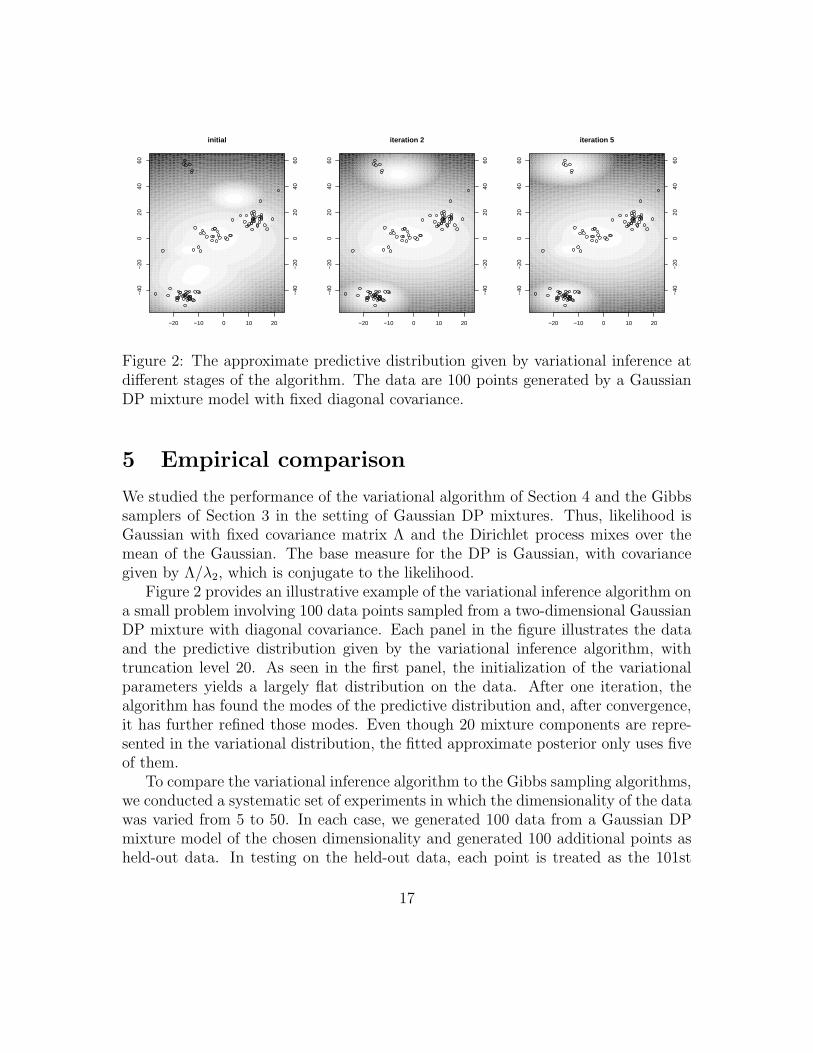
Note that the collapsed Gibbs sampler converged faster than the TDP Gibbssampler. Though an iteration of collapsed Gibbs is slower than an iteration of TDPGibbs, the TDP Gibbs sampler required a longer burn-in and greater lag to obtainuncorrelated samples. This is illustrated in the example autocorrelation plots of Fig-ure 5. Comparing the two MCMC algorithms, we find no advantage to the truncatedapproximation.

Figure 3 (right) illustrates the average log likelihood assigned to the held-outdata by the approximate predictive distributions. First, notice that the collapsed DPGibbs sampler assigned the same likelihood as the posterior from the TDP Gibbssampler—an indication of the quality of a TDP for approximating a DP. More im-portantly, however, the predictive distribution based on the variational posteriorassigned a similar score as those based on samples from the true posterior. Though

19

0 50 100 150

0.0

0.4

0.8

Lag

Aut

ocor

rela

tion

0 50 100 150

0.0

0.4

0.8

Lag

Aut

ocor

rela

tion

Figure 5: Autocorrelation plots on the size of the largest component for the truncatedDP Gibbs sampler (left) and collapsed Gibbs sampler (right) in an example datasetof 50-dimensional Gaussian data.

it is based on an approximation to the true posterior, the resulting predictive distri-butions are very accurate for this class of DP mixtures.

6 Image analysis

Finite Gaussian mixture models are widely used in computer vision to model naturalimages for the purposes of automatic clustering, retrieval, and classification (Barnardet al., 2003; Jeon et al., 2003). These applications are often large-scale data analysisproblems, involving thousands of data points (images) in hundreds of dimensions(pixels). The appropriate number of mixture components to use in these problems isgenerally unknown, and DP mixtures would seem to provide an attractive extensionof current methods. This deployment of DP mixtures in such problems requires,however, inferential methods that are computationally efficient. To demonstratethe applicability of our variational approach to DP mixtures in the setting of largedatasets, we analyzed a collection of 5000 images from the Associated Press underthe assumptions of a Gaussian DP mixture model.

Each image is reduced to a 192-dimensional real-valued vector given by an 8× 8grid of average red, green, and blue values. The overall mean is subtracted to yield adataset with mean zero. We fit a model which is a DP mixture in which the mixturecomponents are Gaussian with mean µ and covariance matrix σ2I. The base measureG0 is a product measure—Gamma(4,2) for σ2 and N (0, 5σ2) for µ. Furthermore, weplace a Gamma(1,1) prior on the DP scaling parameter α, as described in Section 4.1.We use a truncation level of 150 for the variational distribution.

The variational algorithm required approximately 4 hours to converge. The re-sulting approximate posterior uses 79 mixture components to describe the collec-

20

Figure 6: Four sample clusters from a DP mixture analysis of 5000 images fromthe Associated Press. The left-most column is the posterior mean of each clusterfollowed by the top ten images associated with it. These clusters capture patterns inthe data, such as basketball shots, outdoor scenes on gray days, faces, and pictureswith blue backgrounds.

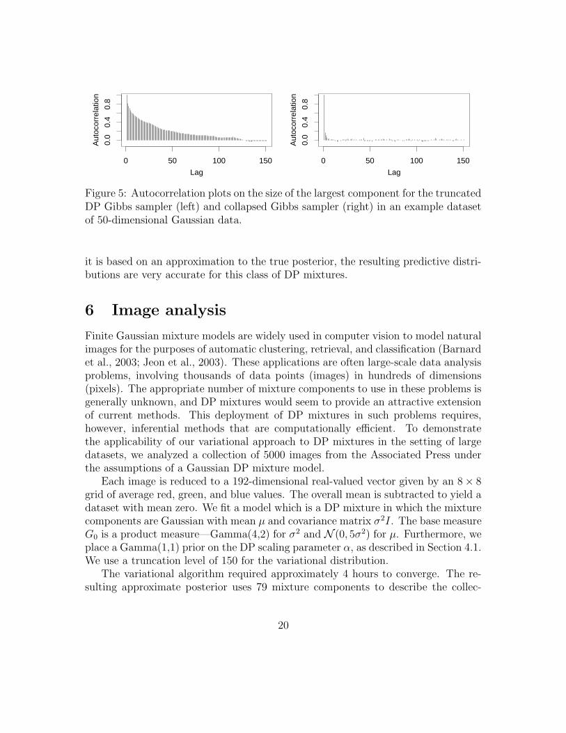
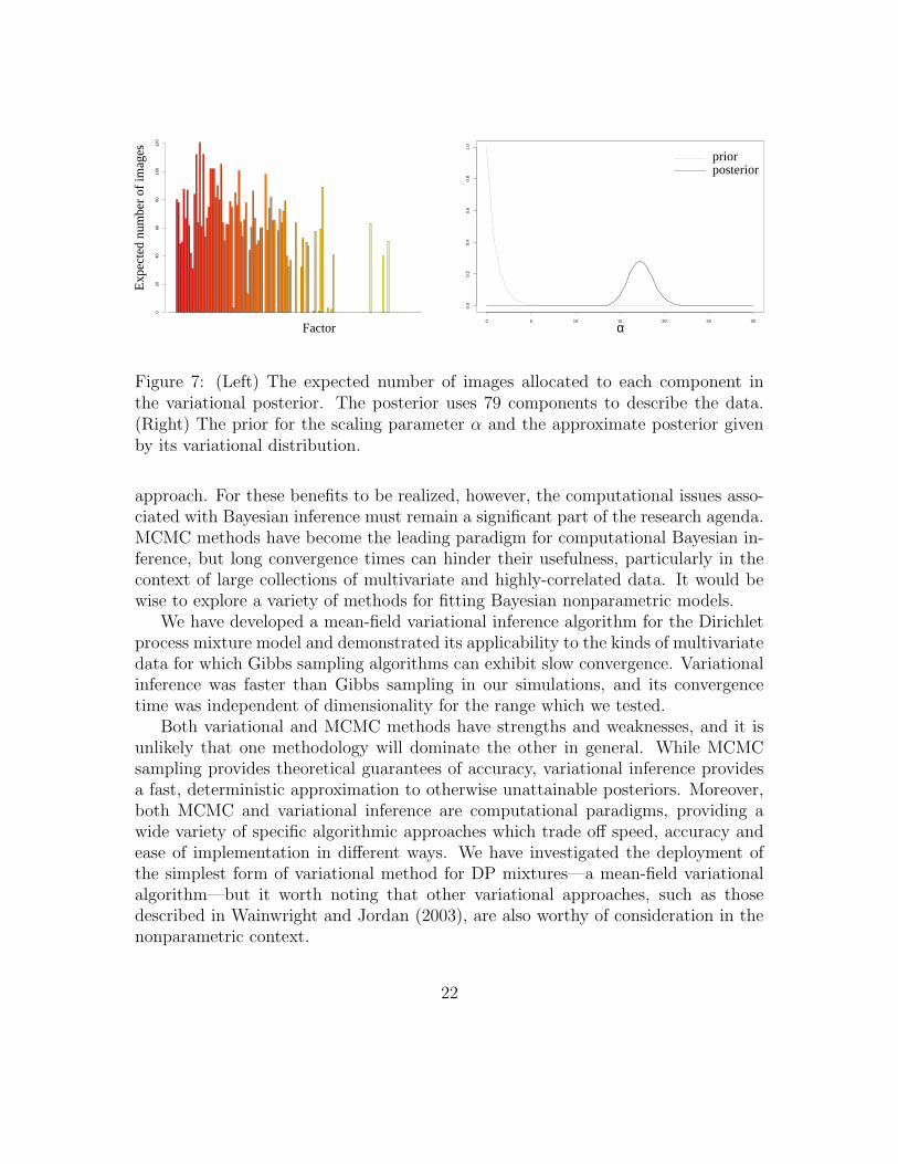
tion. Figure 7 (Left) illustrates the expected number of images allocated to eachcomponent. Figure 6 illustrates the ten pictures with highest approximate posteriorprobability associated with each of four of the components. These clusters appearto capture pictures with basketball shots, outdoor scenes on gray days, faces, andpictures with blue backgrounds.

Figure 7 (Right) illustrates the prior for the scaling parameter α as well as theapproximate posterior given by the fitted variational distribution. We see that theapproximate posterior is peaked and rather different from the prior, indicating thatthe data have provided information regarding α. Moreover, the peak is centeredaround a large value of α, suggesting that the parametric model is inadequate in thiscase.

7 Conclusions

Bayesian nonparametric models based on the Dirichlet process are powerful tools forflexible data analysis. They offer the inferential strengths of the Bayesian approachtogether with a degree of robustness that is not always associated with the Bayesian

21

0 5 10 15 20 25 30

0.0

0.2

0.4

0.6

0.8

1.0

020

4060

8010

012

0priorposterior

Factor

Exp

ecte

d nu

mbe

r of

imag

es

α

Figure 7: (Left) The expected number of images allocated to each component inthe variational posterior. The posterior uses 79 components to describe the data.(Right) The prior for the scaling parameter α and the approximate posterior givenby its variational distribution.

approach. For these benefits to be realized, however, the computational issues asso-ciated with Bayesian inference must remain a significant part of the research agenda.MCMC methods have become the leading paradigm for computational Bayesian in-ference, but long convergence times can hinder their usefulness, particularly in thecontext of large collections of multivariate and highly-correlated data. It would bewise to explore a variety of methods for fitting Bayesian nonparametric models.

We have developed a mean-field variational inference algorithm for the Dirichletprocess mixture model and demonstrated its applicability to the kinds of multivariatedata for which Gibbs sampling algorithms can exhibit slow convergence. Variationalinference was faster than Gibbs sampling in our simulations, and its convergencetime was independent of dimensionality for the range which we tested.

Both variational and MCMC methods have strengths and weaknesses, and it isunlikely that one methodology will dominate the other in general. While MCMCsampling provides theoretical guarantees of accuracy, variational inference providesa fast, deterministic approximation to otherwise unattainable posteriors. Moreover,both MCMC and variational inference are computational paradigms, providing awide variety of specific algorithmic approaches which trade off speed, accuracy andease of implementation in different ways. We have investigated the deployment ofthe simplest form of variational method for DP mixtures—a mean-field variationalalgorithm—but it worth noting that other variational approaches, such as thosedescribed in Wainwright and Jordan (2003), are also worthy of consideration in thenonparametric context.

22

References

Antoniak, C. (1974). Mixtures of Dirichlet processes with applications to Bayesiannonparametric problems. The Annals of Statistics, 2(6):1152–1174.

Attias, H. (2000). A variational Bayesian framework for graphical models. In Solla,S., Leen, T., and Muller, K., editors, Advances in Neural Information ProcessingSystems 12, pages 209–215, Cambridge, MA. MIT Press.

Barnard, K., Duygulu, P., de Freitas, N., Forsyth, D., Blei, D., and Jordan, M.(2003). Matching words and pictures. Journal of Machine Learning Research,3:1107–1135.

Beal, M. (2003). Variational algorithms for approximate Bayesian inference. PhDthesis, Gatsby Computational Neuroscience Unit, University College London.

Bertsekas, D. (1999). Nonlinear Programming. Athena Scientific, Nashua, NH.

Bishop, C., Spiegelhalter, D., and Winn, J. (2003). VIBES: A variational inferenceengine for Bayesian networks. In Becker, S., Thrun, S., and Obermayer, K., editors,Advances in Neural Information Processing Systems 15, pages 777–784. MIT Press,Cambridge, MA.

Blackwell, D. and MacQueen, J. (1973). Ferguson distributions via Polya urnschemes. The Annals of Statistics, 1(2):353–355.

Blei, D., Ng, A., and Jordan, M. (2003). Latent Dirichlet allocation. Journal ofMachine Learning Research, 3:993–1022.

Brown, L. (1986). Fundamentals of Statistical Exponential Families. Institute ofMathematical Statistics, Hayward, CA.

Connor, R. and Mosimann, J. (1969). Concepts of independence for proportions witha generalization of the Dirichlet distribution. Journal of the American StatisticalAssociation, 64(325):194–206.

Escobar, M. and West, M. (1995). Bayesian density estimation and inference usingmixtures. Journal of the American Statistical Association, 90:577–588.

Ferguson, T. (1973). A Bayesian analysis of some nonparametric problems. TheAnnals of Statistics, 1:209–230.

23

Gelfand, A. and Kottas, A. (2002). A computational approach for full nonparametricBayesian inference under Dirichlet process mixture models. Journal of Computa-tional and Graphical Statistics, 11:289–305.

Gelfand, A. and Smith, A. (1990). Sample based approaches to calculating marginaldensities. Journal of the American Statistical Association, 85:398–409.

Geman, S. and Geman, D. (1984). Stochastic relaxation, Gibbs distributions andthe Bayesian restoration of images. IEEE Transactions on Pattern Analysis andMachine Intelligence, 6:721–741.

Ghahramani, Z. and Beal, M. (2001). Propagation algorithms for variationalBayesian learning. In Leen, T., Dietterich, T., and Tresp, V., editors, Advances inNeural Information Processing Systems 13, pages 507–513, Cambridge, MA. MITPress.

Gilks, W., Richardson, S., and Spiegelhalter, D. (1996). Markov chain Monte CarloMethods in Practice. Chapman and Hall.

Ishwaran, J. and James, L. (2001). Gibbs sampling methods for stick-breaking priors.Journal of the American Statistical Association, 96:161–174.

Jeon, J., Lavrenko, V., and Manmatha, R. (2003). Automatic image annotation andretrieval using cross-media relevance models. In Proceedings of the 26th annualinternational ACM SIGIR conference on Research and Development in InformaionRetrieval, pages 119–126. ACM Press.

Jordan, M., Ghahramani, Z., Jaakkola, T., and Saul, L. (1999). Introduction tovariational methods for graphical models. Machine Learning, 37:183–233.

Neal, R. (1993). Probabilistic inference using Markov chain Monte Carlo methods.Technical Report CRG-TR-93-1, Department of Computer Science, University ofToronto.

Neal, R. (2000). Markov chain sampling methods for Dirichlet process mixture mod-els. Journal of Computational and Graphical Statistics, 9(2):249–265.

Opper, M. and Saad, D. (2001). Advanced Mean Field Methods: Theory and Practice.MIT Press, Cambridge, MA.

Raftery, A. and Lewis, S. (1992). One long run with diagnostics: Implementationstrategies for Markov chain Monte Carlo. Statistical Science, 7:493–497.

24

Robert, C. and Casella, G. (1999). Monte Carlo Statistical Methods. Springer Textsin Statistics. Springer-Verlag, New York, NY.

Rockafellar (1970). Convex Analysis. Princeton University Press, Princeton, NJ.

Sethuraman, J. (1994). A constructive definition of Dirichlet priors. Statistica Sinica,4:639–650.

Wainwright, M. and Jordan, M. (2003). Graphical models, exponential families, andvariational inference. Technical Report 649, U.C. Berkeley, Dept. of Statistics.

Wiegerinck, W. (2000). Variational approximations between mean field theory andthe junction tree algorithm. In Boutilier, C. and Goldszmidt, M., editors, Pro-ceedings of the 16th Annual Conference on Uncertainty in Artificial Intelligence(UAI-00), pages 626–633, San Francisco, CA. Morgan Kaufmann Publishers.

Xing, E., Jordan, M., and Russell, S. (2003). A generalized mean field algorithm forvariational inference in exponential families. In Meek, C. and Kjrulff, U., editors,Proceedings of the 19th Annual Conference on Uncertainty in Artificial Intelligence(UAI-03), pages 583–591, San Francisco, CA. Morgan Kaufmann Publishers.

A A conjugate prior for the scaling parameter

In this appendix we show that a gamma prior for the scaling parameter α is conjugateto the stick lengths in the stick-breaking representation of the Dirichlet process.

Recall that the Vn are distributed as Beta(1, α):

p(v |α) = α(1− v)α−1.

Writing this in the canonical exponential family form:

p(v |α) = (1/(1− v)) exp{α log(1− v) + log α},

we see that h(v) = 1/(1− v), t(v) = log(1− v), and a(α) = − log α. Thus, we needa distribution in which t(α) = 〈α, log α〉.

Consider the gamma distribution for α with shape parameter s1 and inverse scaleparameter s2:

p(α | s1, s2) =ss1

2

Γ(s1)αs1−1 exp{−s2α}.

25

In its canonical form the distribution on α is:

p(α | s1, s2) = (1/α) exp{−s2α + s1 log α− a(s1, s2)},

which is conjugate to Beta(1, α). The log normalizer is:

a(s1, s2) = log Γ(s1)− s1 log s2,

and the posterior parameters conditional on data {v1, . . . , vK} are:

s2 = s2 −K∑

i=1

log(1− vi)

s1 = s1 + K.

26