Generative Particle Variational Inference via Estimation of FunctionalGradients

Neale Ratzlaff * 1 Qinxun Bai * 2 Li Fuxin 1 Wei Xu 2

AbstractRecently, particle-based variational inference(ParVI) methods have gained interest becausethey can avoid arbitrary parametric assumptionsthat are common in variational inference. How-ever, many ParVI approaches do not allow arbi-trary sampling from the posterior, and the fewthat do allow such sampling suffer from subop-timality. This work proposes a new method forlearning to approximately sample from the pos-terior distribution. We construct a neural samplerthat is trained with the functional gradient of theKL-divergence between the empirical samplingdistribution and the target distribution, assum-ing the gradient resides within a reproducing ker-nel Hilbert space. Our generative ParVI (GPVI)approach maintains the asymptotic performanceof ParVI methods while offering the flexibilityof a generative sampler. Through carefully con-structed experiments, we show that GPVI outper-forms previous generative ParVI methods suchas amortized SVGD, and is competitive withParVI as well as gold-standard approaches likeHamiltonian Monte Carlo for fitting both exactlyknown and intractable target distributions.

1. IntroductionBayesian inference provides a powerful framework for rea-soning and prediction under uncertainty. However, com-puting the posterior is tractable with only a few parametricdistributions, making wider applications of Bayesian infer-ence difficult. Traditionally, MCMC and variational infer-ence methods are utilized to provide tractable approximateinference, but these approaches face their own difficulties ifthe dimensionality of the space is extremely high. For ex-ample, a recent case of interest is Bayesian neural networks(BNNs), which applies Bayesian inference to deep neural

*Equal contribution 1Department of Electrical Engineering andComputer Science, Oregon State University, Corvallis, Oregon2Horizon Robotics, Cupertino, California. Correspondence to:Neale Ratzlaff <ratzlafn@oregonstate.edu>.

Proceedings of the 38 th International Conference on MachineLearning, PMLR 139, 2021. Copyright 2021 by the author(s).

network training in order to provide a principled way to as-sess model uncertainty. The goal in this regime is to modelthe posterior of every parameter in all the weight tensorsfrom every layer of a deep network. However, develop-ing efficient computational techniques for approximatingthis intractable posterior with extremely high dimensional-ity remains challenging.

Recently, particle-based variational inference (ParVI)methods (Liu & Wang, 2016; Liu et al., 2019; Liu, 2017)have been proposed to represent the variational distribu-tion by a set of particles and update them through a deter-ministic optimization process to approximate the posterior.While achieving both asymptotic accuracy and computa-tional efficiency, ParVI methods are restricted by the fixednumber of particles and lack the ability of drawing newsamples beyond the initial set of particles. To address thisissue, amortized ParVI methods (Wang & Liu, 2016) havebeen proposed to amortize the ParVI gradients in traininga neural sampler. While being flexible in drawing samples,in Sec. 4 we show that amortized ParVI methods cannotmatch the convergence behavior of ParVI methods.

In this work, we propose a generative particle variationalinference (GPVI) approach that addresses those issues.GPVI trains a neural sampler network by directly estimat-ing the functional gradient w.r.t. the KL-divergence be-tween the distribution of generated particles and the tar-get distribution, and pulls it back to update the neural sam-pler. As such it allows the neural sampler to directly gen-erate particles that match the posterior distribution, henceachieving the asymptotic accuracy and computational ef-ficiency of ParVI methods. In figure 1, we show that thepredictive distribution of 1D regression functions sampledfrom GPVI nearly matches that from the ParVI solution,while amortized ParVI fails.

The main computational challenge lies in a reliable esti-mate of the functional gradient that involves the inverse ofthe input-output Jacobian of the neural sampler. Instead ofdirectly computing this term and paying a high computa-tional cost, we introduce a helper network to estimate theinverse Jacobian vector product and train the helper net-work via gradient descent. By alternating between this gra-dient step and the gradient update of the sampler network,the computational cost is distributed over the whole train-

Generative Particle Variational Inference via Estimation of Functional Gradients

ing procedure.

In experiments, our proposed approach achieves compara-ble convergence performance as ParVI methods. It is con-siderably superior than that of amortized ParVI methods,while still allowing efficient sampling from the posterior.By directly applying our approach as a hypernetwork togenerate BNNs, we achieve competitive performance re-garding uncertainty estimation.

In summary, our contributions are three-fold,

• We propose GPVI, a new variational inference ap-proach that trains a neural sampler to generate parti-cles from any posterior distribution. GPVI estimatesthe functional gradient and uses it to update the neuralsampler. It enjoys the asymptotic accuracy and com-putational efficiency of ParVI methods. Comparingwith existing amortized ParVI methods, our approachenjoys the same efficiency and flexibility while show-ing considerable advantage in convergence behavior.

• We design careful techniques for efficient gradient es-timates that address the challenges in approximatingthe product between the inverse of the Jacobian and avector.

• We apply our approach to BNNs and achieve com-petitive uncertainty estimation quality for deep neuralnetworks.

2. Related WorkParVI is a recent class of non-parametric variational infer-ence methods. (Liu & Wang, 2016; Liu, 2017) proposedstein variational gradient descent (SVGD), which deter-ministically updates an empirical distribution of particlestoward the target distribution via a series of sequentiallyconstructed smooth maps. Each map defines a perturba-tion of the particles in the direction of steepest descent to-wards the target distribution under the KL-divergence met-ric. Liu et al. (2019) cast ParVI as a gradient flow on thespace of probability measures P2 equipped with the W2

Wasserstein metric, and proposed ParVI methods GFSDand GFSF by smoothing the density and the function re-spectively. A potential limitation of SVGD and GFSF isthe restriction of the transport maps to an RKHS. The fisherneural sampler (Hu et al., 2018; Grathwohl et al., 2020) liftsthe function space of transportation maps to the space ofL2 functions, and performs a minimax optimization proce-dure to find the optimal perturbation. As a non-parametricapproach, ParVI does not depend on the specific parame-terization of the approximate posterior. ParVI is also moreefficient than MCMC methods due to its deterministic up-dates and gradient-based optimization.

The limitation of ParVI is the inability to draw additional

samples beyond the initial set. To address this limitation,our approach allows for arbitrary draws of new samplesonce the generator is trained. The most notable generativeParVI approach prior to our work was amortized SVGD(Wang & Liu, 2016), which proposed using a generativemodel to approximately sample from the SVGD particledistribution. Amortized SVGD performs a one-step up-date that backpropagates the SVGD gradient back to thegenerator parameters, which is often not optimal. A moredetailed discussion of the differences between our methodand GPVI is presented in Sec. 3.5.

Performing direct Bayesian inference in the weight-spaceof neural networks (Neal, 2012; Buntine & Weigend, 1991;MacKay, 1992) is known to be intractable in the contextof deep learning. Thus, approximations have been formu-lated using Langevin Dynamics (Welling & Teh, 2011; Ko-rattikara Balan et al., 2015), Monte Carlo dropout (Gal &Ghahramani, 2016; Kingma et al., 2015), and variationalinference with mean-field Gaussian priors (Graves, 2011).The variational approximation has been iterated upon ex-tensively. Bayes by Backprop (Blundell et al., 2015) pro-posed an unbiased gradient estimator that allowed for train-ing of deep Bayesian neural networks using the local repa-rameterization trick from Kingma et al. (2015). However,fully factorized Gaussian approximations are insufficient tocapture the complex structure of a high dimensional pos-terior (Yao et al., 2019). As a result, structured approxi-mate posteriors have been proposed using matrix Gaussians(Louizos & Welling, 2016), normalizing flows (Louizos &Welling, 2017; Krueger et al., 2017), and hypernetworks(Pawlowski et al., 2017).

Evaluating the performance of BNNs is difficult, as thereis often no access to the ground truth posterior. Therefore,prior work often considers a “gold-standard” method suchas HMC (Neal et al., 2011), or exact Gaussian processes(Rasmussen, 2003) as a proxy for the true posterior. Whilethese methods set a high bar for BNNs, they are in gen-eral not scalable to large-scale problems. Nonetheless therewere attempts to bring HMC (Strathmann et al., 2015; Chenet al., 2014) and GPs (Wilson et al., 2016; Cheng & Boots,2017; Wang et al., 2019; Hensman et al., 2013; 2015) in therealm of tractability for high dimensional problems.

Variational inference via smooth transport maps is alsoused in normalizing flows (Rezende & Mohamed, 2015).But the transport maps used in normalizing flows and inMarzouk et al. (2016) are bijections which makes themunsuitable for learning distributions over neural networkfunctions.

3. Generative Particle Variational InferenceWe want to learn a parametric generator: fθ : Z → Rd,parameterized by θ, where Z ⊂ Rd is the convex space of

Generative Particle Variational Inference via Estimation of Functional Gradients

(a) HMC (b) SVGD (c) GPVI (d) Amortized SVGD

Figure 1. Predictive uncertainty of methods for a 1-D regression task. (a) HMC predictive posterior matches the uncertainty in thedata; (b) SVGD performs comparably to HMC; (c) Our proposed GPVI performs similarly to SVGD, with the additional capability ofsampling new particles during inference; (d) Amortized SVGD overestimates the uncertainty when the data is sparse.

input noise and x = fθ(z) generates a sample x from aninput noise z. Let q(x) represents the implicit distributionof samples generated by fθ(z), where z ∼ N(0, Id). Letp(x) be the target distribution, we want to solve for fθ thatminimizes the objective KL (q(x)‖p(x)).

Our approach treats this problem from a functional opti-mization perspective, by first computing the functional gra-dient of the objective, and then pulling it back to parameterspace through the function parameterization. In the rest ofthis section we introduce our algorithm in detail and com-pare it with amortized ParVI approaches.

3.1. Functional gradient and its pullbackLet J (f) = KL (q(x)‖p(x)) be the objective, wherex = f(z). If f is injective, by change of variables forprobability measure,

q(x) =pz(z)∣∣∣det(∂f∂z

)∣∣∣ , (1)

where pz(z) is the distribution from which z is sampled.The minimization objective becomes,

J (f) = Ez

− log p(f(z)) + logpz(z)∣∣∣det(∂f∂z

)∣∣∣ . (2)

Consider some function approximation of f , say f = fθ,then the minimization objective becomes,

J (θ) = Ez

− log p(fθ(z)) + logpz(z)∣∣∣det(∂fθ

∂z

)∣∣∣ . (3)

Directly computing the gradient of J (θ) w.r.t. θ involves

not only an inverse of the Jacobian(∂f∂z

)−1, but also sec-

ond derivatives of fθ (see Appendix A for details), whichis overly expensive to compute in practice.

We propose, instead, to first compute the functional gradi-ent of (2) w.r.t. f , i.e., ∇fJ (f), and then back-propagate

it through the generator to get the gradient w.r.t. θ, i.e.,

∇θJ = Ez

[∂f(z)

∂θ∇fJ (f)(z)

]. (4)

The following theorem gives an explicit formula for com-puting the functional gradient ∇fJ (f) when f is cho-sen from a Reproducing kernel Hilbert space (RKHS). Theproof is provided in Appendix A.

Theorem 3.1. Let x = f(z), where z ∼ pz(z), vectorfunction f = (f1, . . . , fd) ∈ Hd with f i ∈ H, where His the RKHS with kernel k(·, ·), Hd is equipped with in-ner product 〈f , g〉Hd =

∑di=1〈f i, gi〉H. For J (f) well-

defined by (2), we have

∇fJ (f)(z) = Ez′

[−∇x log p(x)

∣∣∣∣x=f(z′)

k(z′, z)

−(∂f

∂z′

)−1∇z′k(z′, z)

].

(5)

3.2. Reparameterization of fThere are two considerations for reparameterizing f .

Firstly, in order for the inverse(∂f∂z′

)−1in (5) to be well-

defined, the Jacobian ∂f∂z′ should be a square matrix, i.e.,

input noise z should have the same dimension as the out-put x = f(z). In practice, especially those applicationsinvolving BNNs, each x represents parameters of a sam-pled neural network and therefore can be extremely highdimensional. As a result, a high dimensional f can be com-putationally prohibitive. Secondly, in order for the changeof variables density formula (1) to hold, f needs to be in-jective, which is in general not guaranteed for an arbitraryneural network function.

To overcome the above two concerns, we consider the fol-lowing parameterization,

fθ(z) = gθ

(z(:k)

)+ λz, ∀z ∈ Rd, (6)

where z(:k) ∈ Rk denotes the vector consisting of the firstk components of z, and gθ : Rk → Rd with parameters

Generative Particle Variational Inference via Estimation of Functional Gradients

θ is a much slimmer neural network. In our experiments,gθ is designed with an input dimension k less than 30% thesize of d. For high dimensional open-category experimentswhere d > 60, 000, we use a k of less than 2% of d. Forfθ defined by (6)), the Jacobian is,[∂fθ∂z

]d×d

=

[[∂gθ∂z(:k)

]d×k

∣∣∣∣0d×(d−k)]d×d

+ λId, (7)

where λ is a hyper-parameter. Note that for sufficientlylarge λ, the Jacobian defined by (7) is positive definite.Since the domain Z of z is convex, it is straightforwardto show that fθ defined by (6) is injective. We include theproof in Appendix A.

In practice we set λ to be 1.0 and find it sufficient through-out our experiments.

3.3. Estimating the Jacobian inverseThe main computational challenge of (5) lies in computingthe term

(Jf (z′))−1∇z′k(z′, z), (8)

where Jf (z′) = ∂f∂z′ , especially considering that we need

an efficient implementation for batched z and z′.

Directly evaluating and storing the full Jacobian Jf (z′) foreach z′ of the sampled batch is not acceptable from thestandpoint of either time or memory consumption. Thereexist iterative methods for solving the linear equation sys-tem y = (Jf (z′))

−1∇z′k(z′, z) (Young, 1954; Fletcher,1976), which involves computing the vector-Jacobian prod-uct Jf (z′)∇z′k(z′, z) at each iteration. By alternating be-tween this iterative solver and the gradient update (4), itis possible to get a computationally amenable algorithm.However, as shown in the Appendix C, such an algorithmdoes not converge to the target distribution p even for a sim-ple Bayesian linear regression task. This is due to the factthat batches of both z and z′ for evaluating (5) need to bere-sampled for each gradient update (4) to avoid the cumu-lative sampling error. Therefore, the above alternating pro-cedure of iterative solver for y = (Jf (z′))

−1∇z′k(z′, z)ends up shooting a moving target for different batches of zand z′ at each iterate, which is difficult for convergence.

To overcome this computational challenge, we propose ahelper network, denoted by hη(z′,∇z′k), and parameter-ized by η, that consumes both z′ and∇z′k(z′, z) and pre-dicts (Jf (z′))

−1∇z′k(z′, z). With the helper network, thefunctional gradient (5) can be computed by,

∇fJ (f)(z) = Ez′

[−∇x log p(x)

∣∣∣∣x=f(z′)

k(z′, z)

− hη (z′,∇z′k(z′, z))

].

(9)

We use the following loss to train the helper network,

L(η) = ‖Jf (z′)hη(z′,∇z′k(z′, z))−∇z′k(z′, z)‖2,(10)

where Jf (z′)hη can be computed by the following for-mula given the reparameterization (6) of fθ,

hTη

(∂fθ∂z′

)= hTη

(∂gθ∂z′(:k)

)+ λhTη , (11)

where the Vector-Jacobian Product (VJP) hTη(

∂gθ∂z′(:k)

)can

be computed by one backward pass of the function gθ.

3.4. Summary of the algorithmBoth gθ and hη can be trained with stochastic gradientdescent (SGD), and our algorithm alternates between theSGD updates of gθ and hη . Note that the helper networkhη only has to chase the update of gθ, but no more extramoving targets due to re-sampling of z and z′. Our ex-periments in Sec. 4 and the appendix show that the helpernetwork is able to efficiently approximate (8) which en-ables the convergence of the gradient update (4). Our over-all Generative Particle VI (GPVI) algorithm is summarizedin Algorithm 1.

Algorithm 1 Generative Particle VI (GPVI)Initialize generator gθ, helper hη , and learning rate εwhile Not converge do

1. sample two batches {zi}, {z′i} ∼ N(0, Id)2. compute k(z′, z) and ∇z′k(z′, z)3. forward gθ to compute fθ(z) and fθ(z′) by (6)4. forward hη to compute hη(z′,∇z′k(z′, z))

5. backward gθ to compute the VJP hTη(

∂gθ∂z′(:k)

)and then construct Jf (z′)hη by (11),

6. update hη by η ← η − ε∇ηL,where∇ηL is computed by back-propagating (10)

7. compute the functional gradient by (9)8. update θ by θ ← θ − ε∇θJ ,

where∇θJ is computed by (4)end

3.5. Comparison with Amortized SVGDStein variational gradient descent (SVGD) represents q(x)by a set of particles {xi}ni=1, which are updated iterativelyby,

xi ← xi + εφ∗(xi), (12)

where ε is a step size and φ∗ : Rd → Rd is a vector field(perturbation) on the space of particles that corresponds tothe optimal direction to perturb particles, i.e.,

φ∗ = arg minφ∈F

{d

dεKL(q[εφ](x)‖p(x))

∣∣∣∣ε=0

},

Generative Particle Variational Inference via Estimation of Functional Gradients

where q[εφ](x) denotes the density of particles updatedby (12) using the perturbation φ, where the density of orig-inal particles is q(x). When F is chosen to be the unit ballof some RKHSH with kernel function k(·, ·), SVGD givesthe following closed form solution for φ∗,

φ∗(x) = Ex′∼q [∇x′ log p(x′)k(x′,x) +∇x′k(x′,x)] .(13)

To turn SVGD into a neural sampler, AmortizedSVGD (Wang & Liu, 2016) first samples particles froma generator and then back-propagates the particle gradi-ents (13) through the generator to update the generator pa-rameters. Let x = fθ(z), z ∼ N(0, Id) be the particlegenerating process, where fθ is the generator parameter-ized by θ, amortized SVGD updates θ by,

θ ← θ + ε

m∑i=1

∂fθ(zi)

∂θφ∗(fθ(zi)), (14)

where φ∗(fθ(zi)) is computed by (13).

The following Lemma gives an explicit view regardingwhat functional gradient amortized SVGD back-propagatesthrough the generator. The proof is given in the AppendixA.

Lemma 3.2. If particles are generated by x = f(z), z ∼pz(z), Eqn. (13) is the functional gradient of the KL objec-tive w.r.t. the perturbation function φ : Rd → Rd appliedon the output space of f , i.e.,

∇φ∣∣∣∣φ=id

KL (q(x)‖p(x)) = −φ∗, (15)

where x = φ(f(z)) and φ = (φ1, . . . , φd) ∈ Hd withφi ∈ H, where H is the RKHS with kernel k(·, ·), Hd isequipped with inner product 〈φ, ξ〉Hd =

∑di=1〈φi, ξi〉H.

To see the difference between our GPVI and amortizedSVGD, both methods learn a generator f that generatesparticles x from input noise z. To update f , gradients ofthe KL objective J (f) have to be backpropagated to f inboth cases. Here, the best is to use the steepest descent di-rection for f , which GPVI does (proved in Thm 3.1). AsLemma 3.2 shows, the SVGD gradient φ∗ given by (13) isoptimal for a transformation φ applied to the set of currentparticles. In in both amortized SVGD and GPVI, such a setis not kept and φ does not exist since they only maintainand update f . But amortized SVGD directly uses φ∗(f)in (14) as the direction to update f , which is an unprovenuse – it only coincides with the steepest descent directionfor f used by GPVI in special cases such as f = id,where (5) and (13) are equivalent because z = x and theJacobian is identity. Regarding the definition of RKHS,GPVI’s RKHS approximates the tangent space of f , it istherefore naturally defined on z. (Amortized) SVGD uses

RKHS to approximate the tangent space of φ, which is nat-urally defined on x.

The amortizing step applied in both methods, i.e., back-propagating some functional gradient to update the gener-ator parameters, is in general not guaranteed to keep theoriginal descent direction of the functional gradient. How-ever, GPVI amortizes the steepest descent direction whichis optimal in first order sense, while amortized SVGDamortizes a non-steepest descent direction, which is morelikely to result in a non-descending direction after amortiz-ing. In practice, as shown in the next section, our approachconsistently outperforms amortized SVGD in approximat-ing the target distribution and capturing model uncertainty.

4. ExperimentsTo demonstrate the effectiveness of our approach for ap-proximate Bayesian inference, we evaluated GPVI in twodifferent settings: density estimation and BNNs. In ourdensity estimation experiment, we trained our generatorto draw samples from a target distribution, showing thatGPVI can accurately fit the posterior from the data. Forour BNN experiments, we evaluated on regression, clas-sification, and high dimensional open-category tasks. Ourexperiments show that among all methods compared, GPVIis the only method to excel in both sampling efficiency andasymptotic performance. We compare GPVI with ParVImethods: SVGD (Liu & Wang, 2016), GFSF (Liu et al.,2019), and KSD (Hu et al., 2018; Grathwohl et al., 2020),as well as their corresponding amortized versions. We alsocompared with a mean-field VI approach Bayes by Back-prop (MF-VI) (Blundell et al., 2015), as well as deep en-sembles (Lakshminarayanan et al., 2017), and HMC (Nealet al., 2011). We emphasize that our aim is not to only max-imize the likelihood of generated samples, rather we wantto closely approximate the posterior of parameterized func-tions given the data. Thus, predictions w.r.t data unseenduring training should reflect the epistemic uncertainty ofthe model.

The details of our experimental setup are as follows. Inour BNN experiments, we parameterized samples from thetarget distribution as neural networks with a fixed archi-tecture. In the low dimensional regression and classifica-tion settings, we drew 100 samples from the approximateposterior for both training and evaluation, allowing us toevaluate the predictive mean and variance. For methodswithout a sampler e.g. ParVI and deep ensembles, we ini-tialized a 100 member ensemble. In the high dimensionalopen-category tasks, we instead used 10 samples due to thelarger computation cost. For methods that utilize a hyper-network such as GPVI and amortized ParVI, we used Gaus-sian input noise z ∼ N (0, I) and varied the hypernetworkarchitecture depending on the task. For ParVI and deep

Generative Particle Variational Inference via Estimation of Functional Gradients

Method Σ error (2d) ↓ Σ error (5d) ↓Amortized SVGD 0.10 ± .09 0.37 ± .32Amortized GFSF 0.18 ± .04 0.21 ± .13Amortized KSD 0.28 ± .32 1.68 ± .52

GPVI 0.14 ± .08 0.14 ± .04

Table 1. Comparison of generative Particle VI approaches fordensity estimation of 2d and 5d Gaussian distributions.

ensembles we randomly initialized each member of the en-semble. In all methods except HMC we used the Adamoptimizer (Kingma & Ba, 2014). A detailed description ofnetwork architectures, chosen hyperparameters, and exper-imental settings is given in the appendix.

4.1. Density EstimationWe first evaluate the ability of generative approaches tofit a target distribution from data. We used 2D and 5Dzero mean Gaussian distributions with non-diagonal co-variances as our target distributions. We consider samplernetworks with one hidden layer of width 2 and 5, respec-tively, and input noise with the same dimensionality as theoutput. The error is defined as the difference between thetrue variance and the variance of the sampler output distri-bution WWT − Σ, where W is the weights of the sam-pler. As shown in Table 1, while the estimation problembecomes harder with increased dimension, our approachperforms consistently well while amortized ParVI methodssuffer more or less from a performance drop and all end upinferior to our approach. We have included more densityestimation results in the Appendix.

4.2. Bayesian Linear RegressionWe evaluated all methods on Bayesian linear regression toinvestigate how well each method can fit a unimodal nor-mal distribution over linear function weights. The targetfunction is a linear regressor with parameter vector β ∈Rd, i.e., y = Xβ+ ε, whereX ∼ N (0, Id), ε ∼ N (0, I),and βi ∼ U(0, 1) + 5. We chose such linear Gaussiansettings where we can explicitly compute the target poste-rior p(β|X,y) ∼ N ((XTX)−1XTy,XTX) given ob-servations (X,y), allowing us to numerically evaluate howwell each method fits the target distribution. Each methodwas trained to regress y fromX . For GPVI and amortizedParVI methods that make use of a hypernetwork, we useda linear generator with input noise z ∈ Rd. In this set-ting, the output of a generator with bias b and weights Wfollows the distributionN (b,WWT ), which should matchthe posterior p(β|X,y). For ParVI methods and deep en-sembles, we initialized an ensemble of linear regressorswith d parameters. We computed the mean and covarianceof the learned parameters to measure the quality of poste-rior fit. For MF-VI we chose a standard normal prior onthe weights, and likewise computed the mean and covari-

Method µ error ↓ Σ error ↓SVGD 0.006 ± .0024 0.125 ± .03GFSF 0.003 ± .0014 0.139 ± .07KSD 0.009 ± .0006 0.373 ± .11

Amortized SVGD 0.002 ± .0009 0.158 ± .04Amortized GFSF 0.002 ± .0003 0.209 ± .05Amortized KSD 0.004 ± .0007 0.430 ± .10

MF-VI 0.004 ± .0035 0.303 ± .04Deep Ensemble 0.004 ± .0002 1.0 ± 0

HMC 0.009 ± .0003 0.181 ± .05GPVI 0.002 ± .0007 0.128 ± .04

GPVI Exact Jac 0.002 ± .0004 0.106 ± .07

Table 2. Bayesian linear regression. Reported error is the L2

norm of the difference between the learned mean and covarianceparameters, and the ground truth after 50000 iterations.

ance of weight samples to measure posterior fit. We alsotest a variant of GPVI where we exactly compute the Ja-cobian inverse instead of using our helper network. Weset d = 3 in our experiments. While simple, this quan-titative sanity check is crucial before evaluating on morecomplicated domains where the true posterior is not avail-able. It will be evident in later experiments that the abilityto closely approximate the true posterior under this simplesetup is indicative of performance on higher dimensionaltasks.

Results are shown in table 2. Our GPVI outperforms amor-tized ParVI, MF-VI, and surprisingly even HMC. GPVI isalso very competitive with the best ParVI methods, SVGDand GFSF. We note that GPVI is also competitive with the“Exact-Jac” variant, where we invert the Jacobian explic-itly, instead of using the helper network. This “Exact-Jac”version of GPVI is not scalable, but it serves as a bench-mark to show that our helper network is able to closely ap-proximate the exact solution. Finally, as deep ensembleslacks any mechanism for correctly estimating the covari-ance, it performs poorly as expected.

4.3. Multimodal ClassificationThe previous experiment possesses an analytically knowntarget distribution. However, most problems of in-terest involve distributions without closed-form expres-sions. Therefore, we further tested on a 2-dimensional,4-class classification problem, where each class consistsof samples from one component of a mixture distribu-tion. The mixture distribution is defined as p(x) =∑4i=1N (µi, 0.3), with means µi ∈ {(−2,−2), (−2, 2),

(2,−2), (2, 2)}. We assigned labels yi ∈ {1, 2, 3, 4} ac-cording to the index of the mixture component the sam-ples were drawn from. For this task, samples are weightparameters θ of two-layer neural networks with 10 hid-den units in each layer and ReLU activations, denoted by

Generative Particle Variational Inference via Estimation of Functional Gradients

fθ : R2 → R4.

To train each method, we drew a total of 100 trainingpoints, and 200 testing points from the target distribution.To evaluate the posterior predictive distribution, we drewpoints from a grid spaced from {−10, 10}, then plot thepredictive distribution as measured by the standard devia-tion in predictions among model samples in figure 2.

In this setting, the true posterior p(θ|X, y) is unknown andpast work often relies on “gold-standard” approaches likeHMC to serve as the ground truth. In the previous Bayesianlinear regression tests, however, we saw that HMC wasoutperformed by GPVI as well as ParVI methods SVGDand GFSF. In the current test, intuitively, a “gold-standard”approach should yield a predictive distribution with highvariance (high uncertainty) in regions far from the trainingdata, and low variance (low uncertainty) in regions neareach mixture component. As shown in figure 2, GPVI andSVGD both have higher uncertainty in no-data regions thanHMC, while remaining confident on the training data. Onthe other hand, MF-VI and amortized SVGD both underes-timate the uncertainty. The performance of MF-VI is as ex-pected, as mean-field VI approaches are known to charac-teristically underestimate uncertainty. Results of all meth-ods as well as more tests on an easier 2-class variant areincluded in the Appendix.

4.4. Open CategoryTo evaluate the scalability of our approach we turn to large-scale image classification experiments. In this setting, it isnot possible to exactly measure the accuracy of posteriorfits. We instead utilize the open-category task to test if ouruncertainty estimations can help detect outlier examples.The open category task defines a set of inlier classes thatare seen during training, and a set of outlier classes onlyused for evaluation. While in principle, the content of theoutlier classes can be arbitrary, we use semantically simi-lar outlier classes by splitting the training dataset into inlierand outlier classes. The open-category task is in generalmore difficult than out-of-distribution experiments wheredifferent datasets are used as outlier classes, since distribu-tions of categories from the same dataset may be harder todiscriminate.

We evaluated on the MNIST and CIFAR-10 image datasets,following Neal et al. (2018) to split each dataset into 6 in-lier classes and 4 outlier classes. We performed standardfully supervised training on the 6 inlier classes, and mea-sured uncertainty in the 4 unseen outlier classes. We evalu-ated the uncertainty using two widely-used statistics: areaunder the ROC curve (AUC), and the expected calibrationerror (ECE). The AUC score measures how well a binaryclassifier discriminates between predictions made on inlierinputs, vs predictions made on outlier inputs. A perfect

AUC score of 1.0 indicates a perfect discrimination, whilea score of 0.5 indicates that the two sets of predictions areindistinguishable. ECE partitions predictions into equallysized bins, and computes the L1 difference in expected ac-curacy and confidence between bins, which represents thecalibration error of the bin. ECE computes a weighted av-erage of the calibration error of each bin. Together AUCand ECE tell us how well a model can detect outlier inputs,as well as how well the model fits the training distribution.

MNIST consists of 70,000 grayscale images of handwrit-ten digits at 28x28 resolution, divided into 60,000 train-ing images and 10,000 testing images. We further split thedataset by only using the first six classes for training andtesting. The remaining four classes are only used to com-pute the AUC and ECE statistics. We chose the LeNet-5classifier architecture for all models, and trained for 100epochs. Due to the larger computational burden, we onlyconsider 10 samples from each method’s approximate pos-terior for both training and evaluation. Note that our ap-proach is capable of generating many more, but it wouldbe computationally costly to train much more for ensem-bles and particle VI approaches. For GPVI and amortizedParVI methods we used a 3 layer MLP hypernetwork withlayer widths [256, 512, 1024], ReLU activations, and inputnoise z ∈ R256. We did not test HMC in this setting, as thecomputational demand is too high.

Table 3 shows the results. All RKHS-based methods(GPVI, ParVI, amortized ParVI) as well as deep ensemblesachieve high supervised (“clean“) accuracy with the LeNetarchitecture. MF-VI underfits slightly, while KSD strug-gled to achieve competitive accuracy even after 100 epochs.All methods achieved an AUC over 0.95, but SVGD, GFSFand GPVI have the highest AUC values, respectively. Interms of calibration, GPVI and RKHS-based ParVI meth-ods are the best calibrated. KSD is the worst calibratedmodel, and deep ensembles/MF-VI have middling perfor-mance.

Method Clean AUC↑ ECE ↓SVGD 99.3 .989 ± .001 .001 ± .0002GFSF 99.2 .988 ± .003 .002 ± .0003KSD 97.7 .964 ± .005 .014 ± .0007

Amortized SVGD 99.1 .958 ± .015 .002 ± .0007Amortized GFSF 99.2 .978 ± .005 .004 ± .0013Amortized KSD 97.7 .951 ± .008 .017 ± .0010

MF-VI 98.6 .951 ± .008 .014 ± .0027Deep Ensemble 99.3 .972 ± .002 .008 ± .0060

GPVI 99.3 .988 ± .001 .001 ± .0005

Table 3. Results for open-category classification on MNIST. Weshow the result of standard supervised training (Clean), as wellas AUC and ECE statistics computed from training on a subset ofclasses and testing on the rest of the classes as outliers.

Generative Particle Variational Inference via Estimation of Functional Gradients

(a) GPVI (b) SVGD (c) HMC

(d) Amortized SVGD (e) MF-VI (f) Deep Ensemble

Figure 2. Predictive uncertainty of each method on the 4-class classification task, as measured by the standard deviation between pre-dictions of sampled functions. Regions of high uncertainty are shown as darker, while lighter regions correspond to lower uncertainty.The training data is shown as samples from four unimodal normal distributions. It can be seen that amortized SVGD, MF-VI and deepensembles significantly underestimate the uncertainty in regions with no training data

CIFAR-10 consists of 60,000 RGB images depicting 10object classes at 32x32 resolution, divided into 50,000training images and 10,000 testing images. We adoptedthe same 6 inlier / 4 outlier split used in (Neal et al., 2018)for the open-category setting. For this task we used a CNNwith 3 convolutional layers and two linear layers, which ismuch smaller than SOTA classifiers for CIFAR-10. Thoughthe classification accuracy would suffer, it allows us toclearly evaluate our method without considering interac-tions with architectural components such as BatchNorm orresidual connections. We also used 10 samples from eachmethod’s approximate posterior for training and evaluation.For GPVI and amortized ParVI methods we used the samehypernetwork architecture as in the MNIST setup. Table 4shows the results where it can be seen that our GPVI al-most match the performance of SVGD and GFSF in termsof AUC while doing a bit better on ECE.

4.5. DiscussionMuch of the focus regarding recent work on Bayesian neu-ral networks concerns their performance on open-categoryand out-of-distribution tasks with high dimensional imagedatasets. Instead, we show that our method closely ap-proximates the target posterior, both in tasks where theposterior is explicitly known, as well as when it is in-tractable. The Bayesian linear regression and density es-timation tasks served as sanity checks. Because the poste-

Method Clean AUC ↑ ECE ↓SVGD 80.3 .683 ± .008 .055 ± .004GFSF 80.6 .681 ± .004 .068 ± .012

Amortized SVGD 71.12 .636 ± .018 .073 ± .029Amortized GFSF 71.09 .583 ± .007 .042 ± .029

MF-VI 70.0 .649 ± .006 .016 ± .002Deep Ensemble 73.54 .652 ± .018 .033 ± .011

GPVI 76.2 .677 ± .008 .018 ± .015

Table 4. Open-category classification on CIFAR-10. We show re-sults of standard supervised training (Clean), as well as AUC andECE of each method trained in the open-category setting.

rior was known explicitly, we could quantitatively test howwell each method fit the posterior. For density estimation,GPVI outperforms amortized approaches at matching thetarget covariance (Table 1). In Bayesian linear regression,while the approximation was close for all methods, therewas a clear hierarchy in terms of which types of methodsproduced the tightest approximation (Table 2). GPVI andRKHS-based ParVI achieved the best posterior fit overall,and we see in further experiments that quality of fit here isindicative of performance in more difficult tasks.

The four-class classification problem (Fig. 2), while seem-ingly simple, is particularly difficult for most methods weevaluated since many methods tend to overgeneralize to thecorners. MF-VI underestimates the uncertainty as expected

Generative Particle Variational Inference via Estimation of Functional Gradients

(Yao et al., 2019; Minka, 2001; Bishop, 2006). Notably,amortized SVGD also underestimates the uncertainty witha predictive distribution resembling that of a standard en-semble. We believe this is due to the compounding ap-proximation error explained in Section 3.5, i.e., naivelyback-propagating the Stein variational gradient to updatethe generator is more likely to end up with a non-descentdirection compared with back-propagating the exact func-tional gradient as GPVI. As shown in Fig. 2, the posteriorapproximation of GPVI is tighter, with uncertainty that bet-ter matches the data distribution. SVGD performs the bestin this task, with high uncertainty everywhere except in re-gions near observed data. Surprisingly, GPVI and SVGDoutperform HMC here, with clearly higher uncertainty nearthe corners of the sample space. Note that with the func-tional approximation by neural networks, it is hard to de-termine if the true posterior exactly matches the intuitively“ideal” uncertainty plot where low variance only shows uparound each mixture component. On the other hand, HMCis guaranteed to converge to the true posterior over time(Durmus et al., 2017). Given a fixed computational budget,it is possible that GPVI or SVGD could achieve better per-formance. GPVI also has the extra benefit of the ability todraw additional samples, which is not possible with ParVIor HMC.

Our final experimental setting, open-category, reveals thatGPVI consistently has a higher AUC than all other scal-able sampling approaches. On MNIST, GPVI is among theoverall top performers, together with two ParVI methodsSVGD and GFSF. On CIFAR-10, GPVI is among the toptwo performers in ECE and performs only slightly behindthe two best ParVI methods in AUC. Most importantly,GPVI outperforms with clear margins all amortized ParVImethods on both datasets under all metrics. This is consis-tent with all other qualitative and quantitative experimentswe have conducted, which again shows the advantage ofGPVI over existing generative ParVI methods.

We found that KSD completely failed in CIFAR-10,achieving slightly better than random accuracy. We believethis is due to the way that KSD performs the particle up-date. Where SVGD has a closed form expression for theparticle transportation map, KSD parameterizes it with acritic network that has the input-output dimensionality ofthe particle parameters. Training this critic naturally be-comes difficult when applying to neural network functions.

In the open-category setting, there is added time complex-ity for GPVI relative to amortized methods due to trainingour helper network. Compared to amortized SVGD, theextra time complexity of training GPVI is a constant factorless than 1. In our MNIST experiments, this additive factoris 0.28; in CIFAR-10 experiments, this factor is 0.78. Thedifference in MNIST and CIFAR-10 is due to that the out-

put dimension of the helper network scales with the outputdimension of the generator. We believe this is acceptablegiven the performance gain and the possible real (offlinetraining) applications of GPVI.

5. ConclusionWe have presented a new method that fuses the best as-pects of parametric VI with non-parametric ParVI. GPVIhas asymptotic convergence on par with ParVI. Addition-ally, GPVI can efficiently draw samples from the poste-rior. We also presented a method for efficiently estimatingthe product between the inverse of the Jacobian of a deepnetwork, and a gradient vector. Our experiments showedthat GPVI performs on par with ParVI, and outperformsamortized ParVI and other competing methods in Bayesianlinear regression, a classification task, as well as open-category tasks on MNIST and CIFAR-10. In the future wewant to explore the efficacy of our method applied to largescale tasks like image generation.

AcknowledgementsNeale Ratzlaff and Li Fuxin were partially supportedby the Defense Advanced Research Projects Agency(DARPA) under Contract No. HR001120C0011 andHR001120C0022. Any opinions, findings and conclusionsor recommendations expressed in this material are thoseof the author(s) and do not necessarily reflect the views ofDARPA.

ReferencesBishop, C. M. Pattern recognition and machine learning.

springer, 2006.

Blundell, C., Cornebise, J., Kavukcuoglu, K., and Wierstra,D. Weight uncertainty in neural networks. arXiv preprintarXiv:1505.05424, 2015.

Buntine, W. L. and Weigend, A. S. Bayesian back-propagation. Complex systems, 5(6):603–643, 1991.

Chen, T., Fox, E., and Guestrin, C. Stochastic gradienthamiltonian monte carlo. In International conference onmachine learning, pp. 1683–1691, 2014.

Cheng, C.-A. and Boots, B. Variational inference for gaus-sian process models with linear complexity. In Advancesin Neural Information Processing Systems, pp. 5184–5194, 2017.

Durmus, A., Moulines, E., and Saksman, E. On the con-vergence of hamiltonian monte carlo. arXiv preprintarXiv:1705.00166, 2017.

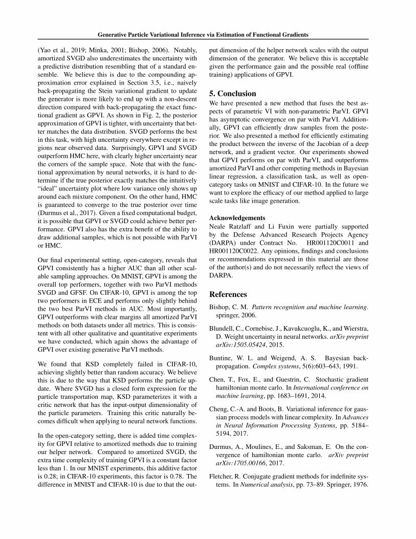
Fletcher, R. Conjugate gradient methods for indefinite sys-tems. In Numerical analysis, pp. 73–89. Springer, 1976.

Generative Particle Variational Inference via Estimation of Functional Gradients

Gal, Y. and Ghahramani, Z. Dropout as a bayesian approx-imation: Representing model uncertainty in deep learn-ing. In international conference on machine learning,pp. 1050–1059, 2016.

Grathwohl, W., Wang, K.-C., Jacobsen, J.-H., Duvenaud,D., and Zemel, R. Learning the stein discrepancyfor training and evaluating energy-based models with-out sampling. In International Conference on MachineLearning, pp. 3732–3747. PMLR, 2020.

Graves, A. Practical variational inference for neural net-works. Advances in neural information processing sys-tems, 24:2348–2356, 2011.

Hensman, J., Fusi, N., and Lawrence, N. D. Gaussianprocesses for big data. arXiv preprint arXiv:1309.6835,2013.

Hensman, J., Matthews, A., and Ghahramani, Z. Scalablevariational gaussian process classification. 2015.

Hu, T., Chen, Z., Sun, H., Bai, J., Ye, M., and Cheng, G.Stein neural sampler. arXiv preprint arXiv:1810.03545,2018.

Kingma, D. P. and Ba, J. Adam: A method for stochasticoptimization. arXiv preprint arXiv:1412.6980, 2014.

Kingma, D. P., Salimans, T., and Welling, M. Varia-tional dropout and the local reparameterization trick. Ad-vances in neural information processing systems, 28:2575–2583, 2015.

Korattikara Balan, A., Rathod, V., Murphy, K. P., andWelling, M. Bayesian dark knowledge. Advances inNeural Information Processing Systems, 28:3438–3446,2015.

Krueger, D., Huang, C.-W., Islam, R., Turner, R., Lacoste,A., and Courville, A. Bayesian hypernetworks. arXivpreprint arXiv:1710.04759, 2017.

Lakshminarayanan, B., Pritzel, A., and Blundell, C. Sim-ple and scalable predictive uncertainty estimation usingdeep ensembles. In Advances in neural information pro-cessing systems, pp. 6402–6413, 2017.

Liu, C., Zhuo, J., Cheng, P., Zhang, R., and Zhu, J. Under-standing and accelerating particle-based variational in-ference. In International Conference on Machine Learn-ing, pp. 4082–4092. PMLR, 2019.

Liu, Q. Stein variational gradient descent as gradient flow.In Advances in neural information processing systems,pp. 3115–3123, 2017.

Liu, Q. and Wang, D. Stein variational gradient descent:A general purpose bayesian inference algorithm. Ad-vances in neural information processing systems, 29:2378–2386, 2016.

Louizos, C. and Welling, M. Structured and efficient vari-ational deep learning with matrix gaussian posteriors.In International Conference on Machine Learning, pp.1708–1716, 2016.

Louizos, C. and Welling, M. Multiplicative normalizingflows for variational bayesian neural networks. arXivpreprint arXiv:1703.01961, 2017.

MacKay, D. J. A practical bayesian framework for back-propagation networks. Neural computation, 4(3):448–472, 1992.

Marzouk, Y., Moselhy, T., Parno, M., and Spantini, A. Anintroduction to sampling via measure transport. arXivpreprint arXiv:1602.05023, 2016.

Minka, T. P. A family of algorithms for approximateBayesian inference. PhD thesis, Massachusetts Instituteof Technology, 2001.

Neal, L., Olson, M., Fern, X., Wong, W.-K., and Li, F.Open set learning with counterfactual images. In Pro-ceedings of the European Conference on Computer Vi-sion (ECCV), pp. 613–628, 2018.

Neal, R. M. Bayesian learning for neural networks, volume118. Springer Science & Business Media, 2012.

Neal, R. M. et al. Mcmc using hamiltonian dynamics.Handbook of markov chain monte carlo, 2(11):2, 2011.

Pawlowski, N., Brock, A., Lee, M. C., Rajchl, M., andGlocker, B. Implicit weight uncertainty in neural net-works. arXiv preprint arXiv:1711.01297, 2017.

Rasmussen, C. E. Gaussian processes in machine learn-ing. In Summer School on Machine Learning, pp. 63–71.Springer, 2003.

Rezende, D. and Mohamed, S. Variational inference withnormalizing flows. In International Conference on Ma-chine Learning, pp. 1530–1538. PMLR, 2015.

Strathmann, H., Sejdinovic, D., Livingstone, S., Szabo, Z.,and Gretton, A. Gradient-free hamiltonian monte carlowith efficient kernel exponential families. Advancesin Neural Information Processing Systems, 28:955–963,2015.

Wang, D. and Liu, Q. Learning to draw samples: Withapplication to amortized mle for generative adversariallearning. arXiv preprint arXiv:1611.01722, 2016.

Generative Particle Variational Inference via Estimation of Functional Gradients

Wang, K., Pleiss, G., Gardner, J., Tyree, S., Weinberger,K. Q., and Wilson, A. G. Exact gaussian processes on amillion data points. In Advances in Neural InformationProcessing Systems, pp. 14648–14659, 2019.

Welling, M. and Teh, Y. W. Bayesian learning via stochas-tic gradient langevin dynamics. In Proceedings ofthe 28th international conference on machine learning(ICML-11), pp. 681–688, 2011.

Wilson, A. G., Hu, Z., Salakhutdinov, R. R., and Xing, E. P.Stochastic variational deep kernel learning. Advances inNeural Information Processing Systems, 29:2586–2594,2016.

Yao, J., Pan, W., Ghosh, S., and Doshi-Velez, F. Qualityof uncertainty quantification for bayesian neural networkinference. arXiv preprint arXiv:1906.09686, 2019.

Young, D. Iterative methods for solving partial differenceequations of elliptic type. Transactions of the AmericanMathematical Society, 76(1):92–111, 1954.