199

Concave Gaussian Variational Approximations for Inference inLarge-Scale Bayesian Linear Models

Edward Challis David BarberComputer Science Department, University College London, London WC1E 6BT, UK.

Abstract

Two popular approaches to forming boundsin approximate Bayesian inference are localvariational methods and minimal Kullback-Leibler divergence methods. For a large classof models we explicitly relate the two ap-proaches, showing that the local variationalmethod is equivalent to a weakened formof Kullback-Leibler Gaussian approximation.This gives a strong motivation to develop ef-ficient methods for KL minimisation. An im-portant and previously unproven property ofthe KL variational Gaussian bound is that itis a concave function in the parameters of theGaussian for log concave sites. This observa-tion, along with compact concave parametri-sations of the covariance, enables us to de-velop fast scalable optimisation procedures toobtain lower bounds on the marginal likeli-hood in large scale Bayesian linear models.

1 BAYESIAN MODELS

For parameter w and data D, a large class of Bayesianmodels describe posteriors of the form

p(w|D) =1

ZN (w µ,Σ)φ(w), (1.1)

Z =

∫N (w µ,Σ)φ(w)dw

for a Gaussian factor N (w µ,Σ) and positive poten-tial function φ(w). This class includes generalised lin-ear models, see e.g. Hardin and Hilbe (2007), andGaussian noise models in inverse modeling, see e.g.Wipf and Nagarajan (2009). A classic example isBayesian logistic regression in which N (w µ,Σ) is the

Appearing in Proceedings of the 14th International Con-ference on Artificial Intelligence and Statistics (AISTATS)2011, Fort Lauderdale, FL, USA. Volume 15 of JMLR:W&CP 15. Copyright 2011 by the authors.

prior on the weight w, φ(w) the likelihood p(D|w) andZ = p(D).

For large parameter dimension, D = dim(w), the nor-malisation constant Z in equation (1.1) is computa-tionally intractable, except for limited special cases.Evaluating Z is essential for the purposes of modelcomparison, hyper-parameter estimation, active learn-ing and experimental design. Indeed, any marginalfunction of the posterior p(w|D), such as a moment,also implicitly requires Z.

Due to the importance of this large model class, agreat deal of effort has been dedicated to finding accu-rate approximations to posteriors of the form equation(1.1). Whilst there are many different possible approx-imation routes, including sampling, consistency meth-ods such as expectation propagation and perturbationtechniques such as Laplace, see e.g. Barber (2011),our interest here is uniquely in techniques that forma lower bound on Z. Such lower bounds are particu-larly useful in parameter estimation and provide con-crete exact knowledge about Z. Furthermore, lowerbounds may be coupled with upper bounds on Z toform bounds on marginal quantities of interest (Gibbsand MacKay, 2000).

A well studied route to forming a lower bound onZ is to use a so-called local variational method thatbounds the integrand with a parametric function, seee.g. Gibbs and MacKay (2000); Jaakkola and Jordan(1996); Girolami (2001); Nickisch and Seeger (2009);Palmer et al. (2006). Local variational optimisationprocedures are, however, computationally demand-ing, requiring the solution of linear systems of di-mension D. For this reason, considerable attentionhas been paid to characterising the convexity of localbounds and developing fast scalable solvers (Nickischand Seeger, 2009; Palmer et al., 2006).

In contrast the Variational Gaussian (VG) method di-rectly approximates the posterior by minimising theKullback-Leibler divergence between a parametrisedGaussian approximation and the posterior. The VGmethod provides a bound on Z for all positive func-

200

Concave Gaussian Variational Approximations for Inference in Large-Scale Bayesian Linear Models

tions φ(w), whilst the local bounding procedure re-quires φ to be super-Gaussian1. Whilst such vari-ational Gaussian (VG) approximations are not new(Barber and Bishop, 1998; Seeger, 1999; Kuss and Ras-mussen, 2005; Opper and Archambeau, 2009), we con-tribute several results concerning this procedure:

• For posteriors in the form of equation (1.1) wemake clear the relationship between local and VGbounds and show that VG bounds are provablytighter than local ones. Furthermore, this im-provement can give rise to differences in the massthey assign to competing models.

• The VG bound has been considered unfavourablecompared to local bounds due to their importantconvexity properties. Here we prove that the VGbound is in fact also concave for log-concave φ.

• The VG method is often dismissed as impracti-cal due to the difficulty of specifying covariancesin large systems. We provide explicit scalableconcave parametrisations for the covariance. Todemonstrate the efficacy of our approach, we ap-ply the method to large datasets, outperformingthe local method in bound value and matching orexceeding it in terms of computational speed.

1.1 Local variational method

The local variational method replaces φ(w) in equa-tion (1.1) with a bound that renders the integral an-alytically tractable. Provided the function φ is super-Gaussian, one may bound φ(w) by an exponentialquadratic function (Palmer et al., 2006)

φ(w) ≥ c(ξ)e− 12wTF(ξ)w+wTf(ξ) (1.2)

where the matrix F(ξ), vector f(ξ) and scalar c(ξ) de-pend on the specific function φ; ξ is a variational pa-rameter that enables one to find the tightest bound.

Many models of practical utility have super-Gaussianpotentials, examples of which are the logistic sigmoidinverse link function φ(x) = (1 + exp(−x))−1, Laplacepotentials where φ(x) ∝ exp(−|x|) and Student’s t-distribution. We discuss explicit c, F and f functionsfor such potentials later, but for the moment leavethem unspecified.

Bounding φ(w) with the squared exponential, we ob-tain

Z ≥ c(ξ) e− 1

2µTΣ−1µ√

det (2πΣ)

∫e−

12wTAw+wTbdw (1.3)

1A function φ(x) is super-Gaussian if ∃b ∈ R s.t. forg(x) := log φ(x)− bx is even, and is convex and decreasingas a function of y = x2 (Seeger and Nickisch, 2010).

where

A ≡ Σ−1 + F(ξ), b ≡ Σ−1µ + f(ξ) (1.4)

Whilst both A and b are functions of ξ, we drop thisdependency for a more compact notation. One caninterpret equation (1.3) as a Gaussian approximationto the posterior where p(w|D) ≈ N

(w A−1b,A−1

).

Completing the square in equation (1.3) and integrat-ing, we have logZ ≥ B(ξ), where

B(ξ) ≡ log c(ξ)− 1

2µTΣ−1µ

+1

2bTA−1b− 1

2log det (ΣA) (1.5)

To obtain the tightest bound on logZ, one then max-imizes B(ξ) with respect to ξ.

In many practical problems of interest, including gen-eralised linear models and inverse modelling,

φ(w) =

N∏n=1

φn(wThn) (1.6)

for local site functions φn and fixed vectors hn. Inthis case, a local bound is applied to each site factorφn. Since the local bounds are all positive, this gives abound dependent on the set of variational parameters

logZ ≥ B(ξ1, . . . , ξN )

The problem of integrating over w has thus been ap-proximated by the requirement to optimise the boundwith respect to the vector ξ of variational parameters.The formal complexity of evaluating the local boundequation (1.5) requires computing det (A) and thus ingeneral scales O

(D3). Furthermore, optimising the

local bound with respect to ξ requires solving a D×Dlinear system N times (Jaakkola and Jordan, 2000;Girolami, 2001).

Such computations are prohibitively expensive whenD � 1, and scalable solvers have recently been de-veloped to address this (Seeger, 2009; Nickisch andSeeger, 2009). The reduced computational burden ofthese methods is principally derived from making tworelaxations. Firstly, double loop algorithms are usedthat, by decoupling the variational bound, reduce thenumber of times that the expensive log det (A) termand its gradient have to be computed. Further sav-ings are obtained by employing low rank approximatefactorisations of A. The computational demand ofthis procedure shifts then from evaluating the gradi-ent of log det (A) to calculating the low K-rank ap-proximate factorisation. This may be achieved usingLanczos codes whose complexity scale super-linearlyin K. The overall resulting complexity of this ‘re-laxed’ local method is both problem and user depen-dent although, roughly speaking, the dimensionality

201

Edward Challis, David Barber

contributes O(D2)

to the complexity of each update.We refer the reader to Nickisch and Seeger (2009) fora detailed discussion. An unfortunate aspect of thisapproximate decomposition is that it does not retaina bound on Z and indeed the quality of the resultingapproximation to Z can be poor.

2 VARIATIONAL GAUSSIANAPPROXIMATION

An alternative to the local bounding method is to fita Gaussian q(w) = N (w m,S) based on minimis-ing KL(q(w)|p(w|D)). Due to the non-negativity ofthe KL divergence, we immediately obtain the boundlogZ ≥ BKL(m,S), where

BKL(m,S) ≡ −〈log q(w)〉+ 〈logN (w µ,Σ)〉+ 〈log φ(w)〉 (2.1)

and 〈·〉 denotes expectation with respect to q(w). ThisVG bound holds for any φ, compared with the lo-cal method which requires φ to be super-Gaussian.An important question, however, is whether the lo-cal bound equation (1.5) or the VG bound equation(2.1) is tighter and, furthermore, how these bounds arerelated. The VG bound has been noted before bothempirically in the case of logistic regression (Nickischand Rasmussen, 2008) and analytically for the spe-cial case of symmetric potentials (Seeger, 2009) to betighter than the local bound. It is also tempting topresume that the VG bound is to be expected to betighter due to the potentially unrestricted covarianceS. In this, however, one needs to bear in mind thatfor local site functions φn, n = 1, . . . , N , providedN > 1

2D(D + 2), the number of variational param-eters in the local method actually exceeds the numberof parameters in the VG method, and such intuitionbreaks down.

2.1 Relating the local and VG bounds

We derive a relationship between the local and VGbounds based on a generic super-Gaussian functionφ(w). We first use the local bound on φ(w), equa-tion (1.2), in equation (2.1) to obtain a new bound

BKL(m,S) ≥ BKL(m,S, ξ)

where2BKL ≡ −2 〈log q(w)〉 − log det (2πΣ) + 2 log c(ξ)

−⟨(w − µ)

TΣ−1(w − µ)

⟩−⟨wTF(ξ)w

⟩+2⟨wTf(ξ)

⟩Using equation (1.4) this can be written as

BKL = −〈log q(w)〉 − 1

2log det (2πΣ) + log c(ξ)

− 1

2µTΣ−1µ− 1

2

⟨wTAw

⟩+⟨wTb

⟩

By defining q(w) = N(w A−1b,A−1

)we obtain

BKL = −KL(q(w)|q(w))−1

2log det (2πΣ)+log c(ξ)

− 1

2µTΣ−1µ +

1

2bTA−1b− 1

2log det (2πA)

Since m,S only appear via q(w) in the KL term, thetightest bound is given when m,S are set such thatq(w) = q(w). At this setting the KL term in BKLdisappears and m and S are given by

Sξ =(Σ−1 + F(ξ)

)−1, mξ = Sξ

(Σ−1µ + f(ξ)

)(2.2)

Since B(m,S) ≥ B(m,S, ξ) we have that,

BKL(mξ,Sξ) ≥ BKL(mξ,Sξ, ξ) = B(ξ) (2.3)

Importantly, the VG bound can be tightened beyondthis setting:

maxm,SBKL(m,S) ≥ BKL(mξ,Sξ) (2.4)

Thus optimal VG bounds are provably tighter thanboth the local variational bound and the VG boundcalculated using the optimal local moments mξ andSξ. The experiments in section(5) show that the im-provement in VG bound values can be significant. Fur-thermore, constrained parametrisations of covariance,which are required when D � 1, are also frequentlyobserved to outperform local variational solutions.

2.2 Tractable VG Approximations

The bound equation (2.1) assumes we can compute〈log φ(w)〉. For generic functions φ, this may not bepractical. However, for the product of site projectionsform, equation (1.6), each projection wThn is Gaus-sian distributed and

I ≡ 〈log φ(w)〉 =∑n

〈log φn(µn + zσn)〉N (z 0,1) (2.5)

with µn ≡ mThn and σ2n ≡ hT

nShn. Hence I can bereadily computed either analytically (for example forφ(x) ∝ e−|x|) or more generally using one-dimensionalnumerical integration (Barber and Bishop, 1998; Kussand Rasmussen, 2005).

A further point of interest is that for local sites, equa-tion (1.6), by differentiating the VG bound with re-spect to S and equating to zero, the optimal form forthe covariance satisfies

S−1 = Σ−1 + HΓHT (2.6)

where Γ is diagonal such that

Γnn =

⟨zφ′n(µn + zσn)

2σnφn(µn + zσn)

⟩(2.7)

202

Concave Gaussian Variational Approximations for Inference in Large-Scale Bayesian Linear Models

and H = [h1, . . . ,hN ]. Here Γ is dependent on Sthrough the projected variance terms σn and we donot have a closed expression or fixed point procedurefor optimising the bound. Unfortunately, optimisingthe bound directly with respect to Γnn is infeasibledue the computational cost of storing and inverting Swhen D and N � 1. Furthermore, S parametrisedin the form of equation (2.6) renders the bound non-concave in Γnn. We shall return to the issue of scalablealternative parametrisations of S in section(4).

3 VG BOUND CONCAVITY

An attractive property of local variational methods isthat they have been proved to be convex problemswhen φ is log-concave (Seeger, 2009). Here we showthat this important property is not restricted to localvariational methods. For log-concave potentials φ(w)of the form equation (1.6), the VG bound BKL(m,S),equation (2.1), is jointly concave with respect to thevariational Gaussian parameters m and S.

In order to show this we parametrise the covarianceS of the variational Gaussian distribution q(w) =N (w m,S) using the Cholesky decomposition S =CCT where C is a square lower triangular matrix ofdimension D. Since the bound depends on the log-arithm of φ, without loss of generality we may takeN = 1, and on ignoring constants with respect to mand S, we have that

BKL(m,C)c.=∑i

logCii−1

2mTΣ−1m+µTΣ−1m

− 1

2trace

(Σ−1CCT

)+⟨log φ(wTh)

⟩(3.1)

Excluding⟨log φ(wTh)

⟩from the expression above, all

terms are concave functions exclusively in either mor C. Since the sum of concave functions on distinctvariables is jointly concave, these terms represent ajointly concave contribution. To complete the proofwe therefore need to show that

⟨log φ(wTh)

⟩is jointly

concave in m and C. We first transform variables towrite

⟨log φ(wTh)

⟩as

〈log φ(a)〉N (a mTh,hTSh) = 〈ψ(µ(m) + zσ(C))〉z (3.2)

where 〈·〉z refers to taking the expectation with respectto the standard normal N (z 0, 1) and,

µ(m) ≡mTh, σ(C) ≡√

hTCCTh, ψ ≡ log φ

Note that establishing the concavity of equation (3.2)is non-trivial since the function ψ(µ(m) + zσ(C)) isitself not jointly concave in C and m.

For ease of notation we let σ′ ≡ vec(∂σ(C)∂C

), where

vec (X) is the vector obtained by concatenating the

columns of X, with dimension D2; σ′′ ≡ ∂2σ(C)∂C2 is

the Hessian of σ with respect to C with dimension

D2×D2; µ′ ≡ ∂µ(m)∂m is a column vector with dimension

D. Then the Hessian of ψ with respect to m and Ccan be expressed in the following block matrix form

H[ψ] =

[∂2ψ∂C2

∂2ψ∂C∂m

∂2ψ∂m∂C

∂2ψ∂m2

]

=

[ψ′′z2σ′σ′

T+ ψ′zσ′′ ψ′′zσ′µ′

T

ψ′′zµ′σ′T

ψ′′µ′µ′T

]

The Hessian of 〈ψ(µ(m) + zσ(C))〉z is equivalentto 〈H[ψ(µ(m) + zσ(C))]〉z, which we now show tobe negative semi-definite. Since the expectation in〈H[ψ(µ(m) + zσ(C))]〉z is with respect to an evenGaussian density function, provided that for all γ ≥ 0,the combined Hessian is negative definite, i.e.

Hz=−γ [ψ] +Hz=+γ [ψ] � 0 (3.3)

then the expectation of H[g] with respect to z is neg-ative definite. To show this we first note that for allu ∈ RD2

and v ∈ RD[uv

]TH[ψ]

[uv

]= ψ′′

[vTµ′ + zuTσ′

]2+ψ′zuTσ′′u

The first term of the right hand side is negative for allvalues of z since ψ′′(x) ≤ 0.

To show that equation (3.3) is satisfied it is sufficientto show that

(ψ′(µ+ γσ)− ψ′(µ− γσ)) γuTσ′′u ≤ 0

which is true since σ′′ � 0, σ(C) ≥ 0 and becauseψ′(x) is a decreasing function from the assumed log-concavity of φ.

To see that σ′′ � 0 we write, σ2(C) =∑j g

2j (C) where

gj(C) = |∑i hiCij | is convex and non-negative for all

j. For convex and non-negative functions gj and p > 1,

then(∑W

j=1 gj(x)p)1/p

is convex (Boyd and Vanden-

berghe, 2004), which reveals that σ(C) is convex onsetting p = 2.

The supplementary material contains a simpler proofkindly provided to us after the conference by M. K.Titsias.

4 VG BOUND OPTIMISATION

Whilst highly desirable, concavity of the VG boundwith respect to m and C does not in itself guaran-tee that optimisation is scalable. Thus an importantpractical consideration is the numerical complexity ofa simple gradient based procedure.

203

Edward Challis, David Barber

Cfull Cband Cchev Csub Csub&band

Comp. O(ND2

)O (NDB) O (NDK) O

(NK2

)O (NKB)

Table 1: Time complexity to evaluate the VG boundand its gradient for each covariance parametrisation.

Answering this question in full generality is complexand we therefore restrict ourselves to considering thecommon case in which Σ = s2I and φ(w) factorises

such that φ(w) =∏Nn=1 φ(hT

nw). Note that manypopular models are in this class, such as inverse modelswith isotropic Gaussian observation noise, and gener-alised linear models with isotropic Gaussian priors.

For Cholesky factorisations C of dimension D × Dthe computational bottleneck in computing the VGbound arises from the projected variational variancesσ2n = ||CThn||2 required in the likelihood term, equa-

tion (2.5). Computing all such terms is O(ND2

).

Whilst this appears prohibitive, this complexity com-pares favourably with the local method in which a sin-gle ξ update involves solving N linear D×D systems,thus scaling O

(ND3

). Note also that in many prob-

lems of interest, the hn are sparse, in which case Dshould be taken as the number of non-zero elements,often � D. Nevertheless, O

(D2)

scaling for the VGmethod can be expensive for very large problems. Forsuch cases, reduced parametrisations of the covarianceS are required, as presented below. These reducedparametrisations increase the problem size to whichthe VG procedure can be applied.

Factor Analysis parametrisations of the form S =ΘΘT +diag

(d2)

can capture the K leading directionsof variance for a D × K dimensional loading matrixΘ. Unfortunately, however, this parametrisation is notof the square Cholesky form in section(3) and indeedrenders the VG bound non-concave. Provided one ishappy to accept convergence to possibly local optima,this is still a useful parametrisation.

4.1 Reduced Concave Parametrisations

Whilst full rank Cholesky parametrisations are opti-mal in terms of achieving the tightest possible VGbound, for D � 1 storing and evaluating the gradi-ent with respect to C is prohibitive. Below we con-sider constrained parametrisations which reduce boththe space and time complexity, whilst preserving con-cavity of the bound.

Banded Cholesky. The simplest option is to con-strain the Cholesky matrix to be banded, that isCij = 0 for i > j+B where B is the bandwidth. Doingso reduces the cost of a single bound/gradient compu-tation to O (NDB), see table(1). Such a parametri-sation however assumes zero covariance between vari-

ables that are indexed out of bandwidth.

Chevron Cholesky. We constrain C such thatCij = Θij when i ≥ j and j ≤ K, Cii = di for i > Kand 0 otherwise. Importantly, this reduced parametri-sation does not exclude modelling any individual co-variates whilst conserving concavity of the bound. Fora Cholesky matrix of this form bound/gradient com-putations scale O (NDK).

Subspace Cholesky. Another reduced parametrisa-tion of the covariance can be obtained by consideringarbitrary rotations of the covariance, S = ECCTET

where E forms an orthonormal basis over RD. Sub-stituting this form of the covariance in equation (3.1)and for Σ = s2I we obtain, up to a constant,

BKL(m,C)c.=∑i

logCii −1

2s2[||C||2 + ||m||2

]+

1

s2µTm +

∑n

〈log φ(µn + zσn)〉z (4.1)

where σn = ||CTEThn||. One may reduce the compu-tational burden by decomposing the square orthonor-mal matrix E into two orthonormal matrices such thatE = [E1,E2] where E1 is D ×K and E2 is D × L forL = (D−K). Then for C = blkdiag (C1, cIL×L), withC1 a K ×K Cholesky matrix,

σ2n = ||CT

1ET1hn||2 + c2(||hn||2 − ||ET

1hn||2)

meaning that only the K eigenvectors in E1 needto be approximated. This effect is due to the as-sumed isotropy of Σ, which can be generalised fornon-isotropic Σ by using a coordinate transformationfor which in the new system, the prior covariance isrendered isotropic. Since terms such as ||hn|| needonly be computed once the complexity of bound andgradient computations scales linearly with K, not D.Further savings can be made if we use only bandedCholesky matrices: for C1 having bandwidth B eachbound evaluation and associated gradient computationscales O (NBK).

The success of this factorisation depends on how wellE1 captures the leading directions of variance. Onesimple approach is to use the leading Principal Com-ponents of the ‘dataset’ H. Another option is to usea two stage procedure in which we first assume C islow bandwidth. After optimisation of the VG boundw.r.t. m and C we then obtain an estimate of the pro-jections µn and σn. These can be used to approximatethe diagonal matrix Γ in equation (2.7). We then seeka rank K approximation to this S. The best rank Kapproximation is given by evaluating the smallest Keigenvectors of Σ−1 + HΓHT. For very large sparseproblems D � 1 we use iterative Lanczos methodsto approximate this, using the methods described in

204

Concave Gaussian Variational Approximations for Inference in Large-Scale Bayesian Linear Models

100 200 300 400 500 600 700−2000

−1800

−1600

−1400

−1200

−1000

−800

K

App

x. M

argi

nal L

ikel

ihoo

d

Local appx.Local VGVG ChevLocal exact

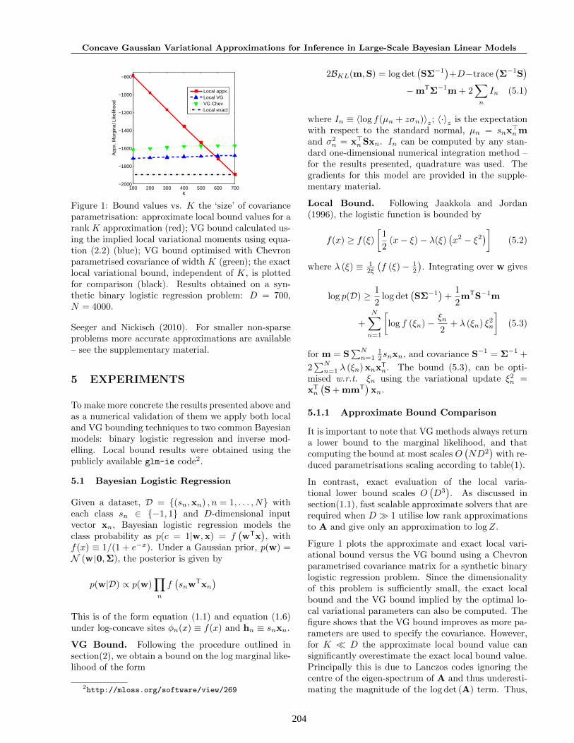
Figure 1: Bound values vs. K the ‘size’ of covarianceparametrisation: approximate local bound values for arank K approximation (red); VG bound calculated us-ing the implied local variational moments using equa-tion (2.2) (blue); VG bound optimised with Chevronparametrised covariance of width K (green); the exactlocal variational bound, independent of K, is plottedfor comparison (black). Results obtained on a syn-thetic binary logistic regression problem: D = 700,N = 4000.

Seeger and Nickisch (2010). For smaller non-sparseproblems more accurate approximations are available– see the supplementary material.

5 EXPERIMENTS

To make more concrete the results presented above andas a numerical validation of them we apply both localand VG bounding techniques to two common Bayesianmodels: binary logistic regression and inverse mod-elling. Local bound results were obtained using thepublicly available glm-ie code2.

5.1 Bayesian Logistic Regression

Given a dataset, D = {(sn,xn) , n = 1, . . . , N} witheach class sn ∈ {−1, 1} and D-dimensional inputvector xn, Bayesian logistic regression models theclass probability as p(c = 1|w,x) = f

(wTx

), with

f(x) ≡ 1/(1 + e−x). Under a Gaussian prior, p(w) =N (w 0,Σ), the posterior is given by

p(w|D) ∝ p(w)∏n

f(snwTxn

)This is of the form equation (1.1) and equation (1.6)under log-concave sites φn(x) ≡ f(x) and hn ≡ snxn.

VG Bound. Following the procedure outlined insection(2), we obtain a bound on the log marginal like-lihood of the form

2http://mloss.org/software/view/269

2BKL(m,S) = log det(SΣ−1

)+D−trace

(Σ−1S

)−mTΣ−1m + 2

∑n

In (5.1)

where In ≡ 〈log f(µn + zσn)〉z; 〈·〉z is the expectationwith respect to the standard normal, µn = snx>nmand σ2

n = x>nSxn. In can be computed by any stan-dard one-dimensional numerical integration method –for the results presented, quadrature was used. Thegradients for this model are provided in the supple-mentary material.

Local Bound. Following Jaakkola and Jordan(1996), the logistic function is bounded by

f(x) ≥ f(ξ)

[1

2(x− ξ)− λ(ξ)

(x2 − ξ2

)](5.2)

where λ (ξ) ≡ 12ξ

(f (ξ)− 1

2

). Integrating over w gives

log p(D) ≥ 1

2log det

(SΣ−1

)+

1

2mTS−1m

+

N∑n=1

[log f (ξn)− ξn

2+ λ (ξn) ξ2n

](5.3)

for m = S∑Nn=1

12snxn, and covariance S−1 = Σ−1 +

2∑Nn=1 λ (ξn) xnxT

n. The bound (5.3), can be opti-mised w.r.t. ξn using the variational update ξ2n =xTn

(S + mmT

)xn.

5.1.1 Approximate Bound Comparison

It is important to note that VG methods always returna lower bound to the marginal likelihood, and thatcomputing the bound at most scales O

(ND2

)with re-

duced parametrisations scaling according to table(1).

In contrast, exact evaluation of the local varia-tional lower bound scales O

(D3). As discussed in

section(1.1), fast scalable approximate solvers that arerequired when D � 1 utilise low rank approximationsto A and give only an approximation to logZ.

Figure 1 plots the approximate and exact local vari-ational bound versus the VG bound using a Chevronparametrised covariance matrix for a synthetic binarylogistic regression problem. Since the dimensionalityof this problem is sufficiently small, the exact localbound and the VG bound implied by the optimal lo-cal variational parameters can also be computed. Thefigure shows that the VG bound improves as more pa-rameters are used to specify the covariance. However,for K � D the approximate local bound value cansignificantly overestimate the exact local bound value.Principally this is due to Lanczos codes ignoring thecentre of the eigen-spectrum of A and thus underesti-mating the magnitude of the log det (A) term. Thus,

205

Edward Challis, David Barber

a9a realsim rcv1

VG

Full

VG

Chev

VG

Sub

Local VG

diag

VG

Chev

VG

Sub

Local VG

diag

VG

Chev

VG

Sub

Local

K − 80 80 80 − 100 750 750 − 50 750 750

Bound −5, 374 −5, 375 −5, 379 −5, 383 −5, 564 −5, 551 −5, 723 − −6, 981 −6, 979 −7, 286 −CPU(s) 85 91 68 5 180 350 575 583 176 424 955 436

Acc. % 15.12 15.10 15.12 15.10 2.86 2.86 2.86 2.87 2.90 2.89 2.94 2.94

Table 2: Approximate local and VG results for the a9a, realsm and rcv1 binary classification tasks. Boundvalues in all cases are evaluated using the VG form. K refers to the ‘rank’ of the approximation: VG Chev Θis D ×K; VG Sub parametrisation uses K dimensional subspace and a diagonal Cholesky matrix; approximatelocal method with K Lanczos vectors. VG diag refers to a bandwidth 1 Cholesky matrix. CPU times wererecorded in MATLAB using an Intel 2.5Ghz Core 2 Quad processor.

in problems of sufficiently large dimensionality, wherenecessarily K � D, local approximate bound valuescannot be relied upon to assess model fidelity. In con-trast the VG procedure offers an exact lower boundon the marginal likelihood that scales according totable(1).

5.1.2 Large Scale Numerical Results

To demonstrate the scalability of the VG method wecompare the performance against fast local methodson three large scale binary classification tasks3, a9a,realsim and rcv1.

Training (tr) and test sets (tst) were randomly par-titioned such that: a9a D = 123, tr = 16, 000,tst = 16, 561 with the number of non zero elements(nnz) totalling nnz = 451, 592 ; realsim D = 20, 958,tr = 36, 000, tst = 36, 309 and nnz = 3, 709, 083;rcv1 D = 42, 736, tr = 50, 000, tst = 50, 000 andnnz = 7, 349, 450.

Model parameters and local optimisation procedureswere, for the purposes of comparison, fixed to the val-ues stated in Nickisch and Seeger (2009): τ , a scal-ing on the likelihood term p(cn|xn) = f(τwTxn), wasset to 1 in the a9a dataset and τ = 3 for realsim

and rcv1; the prior variance was fixed Σ = s2I withs2 = 1. The VG bound was optimised using a conju-gate gradients procedure.

Results for various concave parametrisations of covari-ance are presented in table(2). Local VG bound valuesare not presented for the larger problems since evaluat-ing m and S using equation (2.2) and the optimal localvariational parameters is not computationally feasible,whilst the approximate local bound values are too in-accurate to make meaningful comparisons (see fig(1)).The local bound value for the a9a data set was ob-tained by translating the returned optimal local pa-rameter ξ to a VG Gaussian using equation (2.2). This

3www.csie.ntu.edu.tw/~cjlin/libsvmtools/datasets

VG Gaussian is guaranteed to provide a higher boundthan the local method itself.

Whilst the local method is significantly faster for thesmall D problem a9a (albeit with a worse bound) thanthe VG method, this is due only to different over-heads in the corresponding implementations. In thelarger problems, the results show that a simple VGgradient based optimisation procedure, coupled withconstrained parametrisations of the covariance, canachieve results in terms of speed and accuracy on apar with or in excess of fast local solvers.

5.2 Bayesian Inverse Modelling

Bayesian inverse modelling assumes an observed realvector y ∈ RN is drawn from the generative modely = Mw + η for w ∈ RD, for a model matrix M ofdimension N ×D with N � D and additive sphericalGaussian noise η ∼ N

(0, s2I

). Sparsity can be im-

posed on the inferred object by using a prior of theform φ(w) ≡

∏i p(wi), where each p(wi) is super-

Gaussian. Given y, the posterior is then of the form

p(w|y) =1

ZN(y Mw, s2I

)φ(w) (5.4)

Due to the symmetry N (w µ,Σ) ≡ N (µ w,Σ), andsince M is a linear operator, then provided that φ(w)is log-concave, the arguments of section(3) apply. ForLaplace sparsity priors φ(w) =

∏i

12τie−|wi|/τi both

the VG and local bounds are concave.

VG bound. Following the procedure outlined insection(2) we obtain the following bound on themarginal likelihood,

2BKL(m,S) ≡ −N log(2πs2) + 2

D∑i=1

〈log p(wi)〉

− 1

s2[||y||2 − 2yTMm + ||CTM||2 + ||Mm||2

]+ 2 log det (2πC) +D (5.5)

Evaluating the integral 〈log p(w)〉q(w) in this case isanalytic, the precise form of which, including vari-ational gradients, is presented in the supplementary

206

Concave Gaussian Variational Approximations for Inference in Large-Scale Bayesian Linear Models

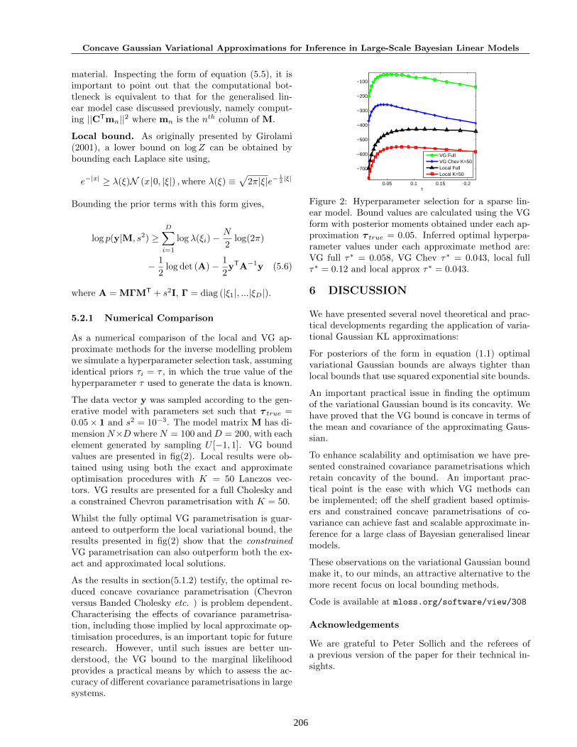
material. Inspecting the form of equation (5.5), it isimportant to point out that the computational bot-tleneck is equivalent to that for the generalised lin-ear model case discussed previously, namely comput-ing ||CTmn||2 where mn is the nth column of M.

Local bound. As originally presented by Girolami(2001), a lower bound on logZ can be obtained bybounding each Laplace site using,

e−|x| ≥ λ(ξ)N (x 0, |ξ|) ,where λ(ξ) ≡√

2π|ξ|e− 12 |ξ|

Bounding the prior terms with this form gives,

log p(y|M, s2) ≥D∑i=1

log λ(ξi)−N

2log(2π)

− 1

2log det (A)− 1

2yTA−1y (5.6)

where A = MΓMT + s2I, Γ = diag (|ξ1|, ...|ξD|).

5.2.1 Numerical Comparison

As a numerical comparison of the local and VG ap-proximate methods for the inverse modelling problemwe simulate a hyperparameter selection task, assumingidentical priors τi = τ , in which the true value of thehyperparameter τ used to generate the data is known.

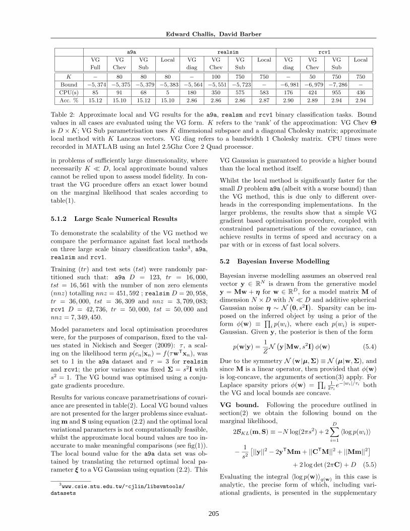
The data vector y was sampled according to the gen-erative model with parameters set such that τ true =0.05× 1 and s2 = 10−3. The model matrix M has di-mensionN×D whereN = 100 andD = 200, with eachelement generated by sampling U [−1, 1]. VG boundvalues are presented in fig(2). Local results were ob-tained using using both the exact and approximateoptimisation procedures with K = 50 Lanczos vec-tors. VG results are presented for a full Cholesky anda constrained Chevron parametrisation with K = 50.

Whilst the fully optimal VG parametrisation is guar-anteed to outperform the local variational bound, theresults presented in fig(2) show that the constrainedVG parametrisation can also outperform both the ex-act and approximated local solutions.

As the results in section(5.1.2) testify, the optimal re-duced concave covariance parametrisation (Chevronversus Banded Cholesky etc. ) is problem dependent.Characterising the effects of covariance parametrisa-tion, including those implied by local approximate op-timisation procedures, is an important topic for futureresearch. However, until such issues are better un-derstood, the VG bound to the marginal likelihoodprovides a practical means by which to assess the ac-curacy of different covariance parametrisations in largesystems.

0.05 0.1 0.15 0.2

−700

−600

−500

−400

−300

−200

−100

τ

VG FullVG Chev K=50Local FullLocal K=50

Figure 2: Hyperparameter selection for a sparse lin-ear model. Bound values are calculated using the VGform with posterior moments obtained under each ap-proximation τ true = 0.05. Inferred optimal hyperpa-rameter values under each approximate method are:VG full τ∗ = 0.058, VG Chev τ∗ = 0.043, local fullτ∗ = 0.12 and local approx τ∗ = 0.043.

6 DISCUSSION

We have presented several novel theoretical and prac-tical developments regarding the application of varia-tional Gaussian KL approximations:

For posteriors of the form in equation (1.1) optimalvariational Gaussian bounds are always tighter thanlocal bounds that use squared exponential site bounds.

An important practical issue in finding the optimumof the variational Gaussian bound is its concavity. Wehave proved that the VG bound is concave in terms ofthe mean and covariance of the approximating Gaus-sian.

To enhance scalability and optimisation we have pre-sented constrained covariance parametrisations whichretain concavity of the bound. An important prac-tical point is the ease with which VG methods canbe implemented; off the shelf gradient based optimis-ers and constrained concave parametrisations of co-variance can achieve fast and scalable approximate in-ference for a large class of Bayesian generalised linearmodels.

These observations on the variational Gaussian boundmake it, to our minds, an attractive alternative to themore recent focus on local bounding methods.

Code is available at mloss.org/software/view/308

Acknowledgements

We are grateful to Peter Sollich and the referees ofa previous version of the paper for their technical in-sights.

207

Edward Challis, David Barber

References

D. Barber. Bayesian Reasoning and Machine Learn-ing. Cambridge University Press, 2011.

D. Barber and C. Bishop. Ensemble Learning inBayesian Neural Networks. In Neural Networks andMachine Learning, pages 215–237. Springer, 1998.

S. Boyd and L. Vandenberghe. Convex Optimization.Cambridge University Press, 2004.

M. Gibbs and D. MacKay. Variational Gaussian Pro-cess Classifiers. IEEE Transactions on Neural Net-works, 11(6):1458–1464, 2000.

M. Girolami. A Variational Method for LearningSparse and Overcomplete Representations. NeuralComputation, 13(11):2517–2532, 2001.

J. Hardin and J. Hilbe. Generalized Linear Models andExtensions. Stata Press, 2007.

T. Jaakkola and M. Jordan. A variational approachto Bayesian logistic regression problems and theirextensions. In Artificial Intelligence and Statistics,1996.

T. Jaakkola and M. Jordan. Bayesian parameter esti-mation via variational methods. Statistics and Com-puting, 10(1):25–37, 2000.

M. Kuss and C. Rasmussen. Assessing ApproximateInference for Binary Gaussian Process Classifica-tion. Journal of Machine Learning Research, 6:1679–1704, 2005.

H. Nickisch and C. Rasmussen. Approximations forBinary Gaussian Process Classification. Journal ofMachine Learning Research, 9:2035–2078, 10 2008.

H. Nickisch and M. Seeger. Convex VariationalBayesian Inference for Large Scale Generalized Lin-ear Models. International Conference on MachineLearning, 26:761–768, 2009.

M. Opper and C. Archambeau. The Variational Gaus-sian Approximation Revisited. Neural Computation,21(3):786–792, 2009.

A. Palmer, D. Wipf, K. Kreutz-Delgado, and B. Rao.Variational EM algorithms for non-Gaussian latentvariable models. In B. Scholkopf, J. Platt, andT. Hoffman, editors, Advances in Neural Informa-tion Processing Systems (NIPS), number 19, pages1059–1066, Cambridge, MA, 2006. MIT Press.

M. Seeger. Bayesian Model Selection for Support Vec-tor Machines, Gaussian Processes and other Ker-nel Classifiers. In S. Solla, T. Leen, and Muller,editors, Advances in Neural Information ProcessingSystems (NIPS), number 12, pages 603–609, Cam-bridge, MA, 1999. MIT Press.

M. Seeger. Sparse linear models: Variational approx-imate inference and Bayesian experimental design.Journal of Physics: Conference Series, 197(1), 2009.

M. Seeger and H. Nickisch. Large Scale Varia-tional Inference and Experimental Design for SparseGeneralized Linear Models. Technical report,Max Planck Institute for Biological Cybernetics,http://arxiv.org/abs/0810.0901, 2010.

D. Wipf and S. Nagarajan. A unified Bayesian frame-work for MEG/EEG source imaging. NeuroImage,44(3):947–966, 2009.