VARIATIONAL INEQUALITIES WITH APPLICATIONS
230
For other titles published in this series, go to www.springer.com/series/5613 VARIATIONAL INEQUALITIES WITH APPLICATIONS
Transcript of VARIATIONAL INEQUALITIES WITH APPLICATIONS

For other titles published in this series, go towww.springer.com/series/5613
VARIATIONAL INEQUALITIES
WITH APPLICATIONS

Advances in Mechanics and Mathematics
Series Editors David Y. Gao (Virginia Polytechnic Institute and State University) Ray W. Ogden (University of Glasgow)
Advisory Board Ivar Ekeland (University of British Columbia, Vancouver) Tim Healey (Cornell University, USA) Kumbakonam Rajagopal (Texas A&M University, USA) Tudor Ratiu (École Polytechnique Fédérale, Lausanne)
David J. Steigmann (University of California, Berkeley)
Aims and Scope Mechanics and mathematics have been complementary partners since Newton’s time, and the history of science shows much evidence of the beneficial influence of these disciplines on each other. The discipline of mechanics, for this series, includes relevant physical and biological phenomena such as: electromagnetic, thermal, quantum effects, biomechanics, nanomechanics, multiscale modeling, dynamical systems, optimization and control, and computational methods. Driven by increasingly elaborate modern technological applications, the symbiotic relationship between mathematics and mechanics is continually growing. The increasingly large number of specialist journals has generated a complementarity gap between the partners, and this gap continues to widen. Advances in Mechanics
and Mathematics is a series dedicated to the publication of the latest developments in the interaction between mechanics and mathematics and intends to bridge the gap by providing interdisciplinary publications in the form of monographs, graduate texts, edited volumes, and a special annual book consisting of invited survey articles.
VOLUME 18

By
A Study of Antiplane Frictional Contact Problems
MIRCEA SOFONEAUniversité de Perpignan, France
ANDALUZIA MATEIUniversity of Craiova, Romania
VARIATIONAL INEQUALITIES
WITH APPLICATIONS

Series Editors:
David Y. Gao Ray W. Ogden Department of Mathematics Department of Mathematics Virginia Tech University of Glasgow Blacksburg, VA 24061 Glasgow, Scotland, UK [email protected] [email protected]
All rights reserved. This work may not be translated or copied in whole or in part without the writtenpermission of the publisher (Springer Science+Business Media, LLC, 233 Spring Street, New York,NY 10013, USA), except for brief excerpts in connection with reviews or scholarly analysis. Use in connection with any form of information storage and retrieval, electronic adaptation, computer software, or by similar or dissimilar methodology now known or hereafter developed is forbidden.
subject to proprietary rights. Printed on acid-free paper springer.com
The use in this publication of trade names, trademarks, service marks, and similar terms, even if they are not identified as such, is not to be taken as an expression of opinion as to whether or not they are
Université de Perpignan
Andaluzia Matei
University of Craiova200585 [email protected]
ISBN: 978-0-387-87459-3 DOI: 10.1007/978-0-387-87460-9
e-ISBN: 978-0-387-87460-9
Library of Congress Control Number:
Mathematics Subject Classification (2000): 58E35, 58E50, 49J40, 49J45, 74M10, 74M15, 74G25,
74G30, 74M99
2008944205
Mircea Sofonea
© Springer Science+Business Media, LLC 2009
ISSN: 1571-8689
Department of MathematicsLaboratoire LAMPS
66 860 Perpignan Cedex

To my teachers Nicolae Cristescu, Caius Iacob,and Gheorghe Popescu, with gratitude
(Mircea Sofonea)
To Claudiu, Alexandru, and Robert, with love
(Andaluzia Matei)
As any human activity needs goals, mathematical research needs problems.—David Hilbert
Mechanics is the paradise of mathematical sciences.—Leonardo da Vinci
Series Preface
Mechanics and mathematics have been complementary partners since New-ton’s time, and the history of science shows much evidence of the beneficialinfluence of these disciplines on each other. Driven by increasingly elabo-rate modern technological applications, the symbiotic relationship betweenmathematics and mechanics is continually growing. However, the increasinglylarge number of specialist journals has generated a duality gap between thepartners, and this gap is growing wider.
Advances in Mechanics and Mathematics (AMMA) is intended to bridgethe gap by providing multidisciplinary publications that fall into the twofollowing complementary categories:
1. An annual book dedicated to the latest developments in mechanics andmathematics;
2. Monographs, advanced textbooks, handbooks, edited volumes, and selectedconference proceedings.
The AMMA annual book publishes invited and contributed comprehensiveresearch and survey articles within the broad area of modern mechanics andapplied mathematics. The discipline of mechanics, for this series, includesrelevant physical and biological phenomena such as: electromagnetic, ther-mal, and quantum effects, biomechanics, nanomechanics, multiscale model-ing, dynamical systems, optimization and control, and computation methods.Especially encouraged are articles on mathematical and computational mod-els and methods based on mechanics and their interactions with other fields.All contributions will be reviewed so as to guarantee the highest possible sci-entific standards. Each chapter will reflect the most recent achievements inthe area. The coverage should be conceptual, concentrating on the method-ological thinking that will allow the nonspecialist reader to understand it.Discussion of possible future research directions in the area is welcome.
vii

viii Series Preface
Thus, the annual volumes will provide a continuous documentation of themost recent developments in these active and important interdisciplinaryfields. Chapters published in this series could form bases from which possibleAMMA monographs or advanced textbooks could be developed.
Volumes published in the second category contain review/research contri-butions covering various aspects of the topic. Together these will provide anoverview of the state-of-the-art in the respective field, extending from an in-troduction to the subject right up to the frontiers of contemporary research.Certain multidisciplinary topics, such as duality, complementarity, and sym-metry in mechanics, mathematics, and physics are of particular interest.
The Advances in Mechanics and Mathematics series is directed to all sci-entists and mathematicians, including advanced students (at the doctoraland postdoctoral levels) at universities and in industry who are interested inmechanics and applied mathematics.
David Y. GaoRay W. Ogden

Preface
The theory of variational inequalities plays an important role in the studyof both the qualitative and numerical analysis of nonlinear boundary valueproblems arising in mechanics, physics, and engineering science. For this rea-son, the mathematical literature dedicated to this field is extensive, and theprogress made in the past four decades is impressive. A part of this progresswas motivated by new models arising in contact mechanics. At the heart ofthis theory is the intrinsic inclusion of free boundaries in an elegant mathe-matical formulation.
Contact between deformable bodies abounds in industry and everyday life.Because of the industrial importance of the physical processes that take placeduring contact, a considerable effort has been made in their modeling, analy-sis, numerical analysis and numerical simulations, and, as a result, the math-ematical theory of contact mechanics has made impressive progress recently.Owing to their inherent complexity, contact phenomena lead to mathematicalmodels expressed in terms of strongly nonlinear evolutionary problems.
Antiplane shear deformations are one of the simplest classes of deforma-tions that solids can undergo: in antiplane shear (or longitudinal shear) of acylindrical body, the displacement is parallel to the generators of the cylin-der and is independent of the axial coordinate. For this reason, the antiplaneproblems play a useful role as pilot problems, allowing for various aspects ofsolutions in solid mechanics to be examined in a particularly simple setting.In recent years, considerable attention has been paid to the analysis of suchkinds of problems.
The purpose of this book is to introduce to the reader the theory of vari-ational inequalities with emphasis on the study of contact mechanics and,more specifically, with emphasis on the study of antiplane frictional contactproblems. The contents cover both abstract results in the study of varia-tional inequalities as well as the study of specific antiplane frictional contactproblems. This includes their modeling and variational analysis. Our inten-tion is to illustrate the cross-fertilization between modeling and applicationson the one hand, and nonlinear mathematical analysis on the other hand.
ix

x Preface
Thus, within the particular setting of antiplane shear, we show how new andnonstandard models in contact mechanics lead to new types of variationalinequalities and, conversely, we show how the abstract results on variationalinequalities can be applied to prove the unique solvability of the correspond-ing contact problems. In writing this book, our aim was also to draw the atten-tion of the applied mathematics community to interesting two-dimensionalmodels arising in solid mechanics, involving a single nonlinear partial differen-tial equation that has the virtue of relative mathematical simplicity withoutloss of essential physical relevance.
Our book, divided into four parts with 11 chapters, is intended as a uni-fied and readily accessible source for mathematicians, applied mathemati-cians, engineers, and scientists, as well as advanced graduate students. It isorganized with two different aims, so that readers who are not interested inmodeling and applications can skip Parts III and IV and will find an elemen-tary introduction to the theory of variational inequalities in Part II of thebook; alternatively, readers who are interested in modeling and applicationswill find in Parts III and IV the mechanical models that lead to the variousclasses of variational inequalities presented in Part II of the book.
A brief description of the parts of the book follows.
Part I is devoted to the basic notation and results that are fundamentalto the developments later in this book. We review the background on func-tional analysis and function spaces that we need in the study of variationalinequalities. The material presented is standard and can be found in manytextbooks and monographs. For this reason, we present only very few detailsof the proofs.
Part II represents one of the main parts of the book and includes originalresults. We present various classes of variational inequalities for which weprove existence results and, for some of them, we prove uniqueness, regu-larity, and convergence results. To this end we use convexity, monotonicity,compactness, time discretization, regularization, and fixed point arguments.Most of the concepts and results presented in this part can be extended tomore general variational inequalities involving nonlinear operators on reflex-ive Banach spaces or to hemivariational inequalities; however, since our aimis to provide an accessible presentation of the theory of variational inequali-ties with emphasis in the study of antiplane frictional contact problems, werestrict ourselves to the framework of Hilbert spaces, linear operators, andconvex analysis, as is sufficient for later development.
The terminology we use in this part of book is the following: if the timederivative of the unknown function u appears in the formulation of a vari-ational inequality (and, therefore, an initial condition for u is needed), werefer to it as an evolutionary variational inequality. Otherwise, we refer to itas an elliptic variational inequality. If the nondifferentiable convex functionalj depends explicitly on u or on its time derivative u, we refer to the corre-sponding variational inequality as a quasivariational inequality. If both thedata and the solution of a variational inequality depend on the time variable

Preface xi
that plays the role of a parameter, the corresponding variational inequalityis called a time-dependent variational inequality. Finally, if an integral termcontaining the solution or its derivative appears in the formulation of a vari-ational inequality, we refer to it as a history-dependent variational inequality.This classification is not strict and is intended to distinguish among thetypes of variational inequalities used in the mathematical theory of contactmechanics, as it is illustrated in Part IV.
Part III presents preliminary material of contact mechanics that is neededin the rest of the book. We summarize basic notions and equations of mechan-ics of continua, then we introduce the frictional contact conditions as well asthe constitutive laws that are used in the rest of the book. We then specializethe equations and conditions in the context of the antiplane shear and, as anexample, we study a displacement-traction problem involving linearly elasticmaterials. The material presented in this part provides the background forthe modeling of the antiplane frictional contact problems studied in Part IVof the book.
Part IV represents the other main part of the book and is partially basedon our original research. It deals with the study of static and quasistaticfrictional antiplane contact problems. We model the material behavior withisotropic linearly elastic and viscoelastic constitutive laws and, in the case ofviscoelastic materials, we consider both short and long memory. Friction ismodeled with versions of Coulomb’s law in which the friction bound is eithera function that does not depend on the process variables or depends on theslip or slip rate. Particular attention is paid to history-dependent frictionalproblems in which the friction bound depends on the total slip or the totalslip rate. For each one of the problems, we provide a variational formulationthen we use the abstract results in Part II in order to establish existence andsometimes uniqueness, regularity, and convergence results.
Each of the four parts of the book is divided into several chapters. Allthe chapters are numbered consecutively. Mathematical relations (equalities,inequalities, and inclusions) are numbered by chapter and their order of oc-currence. For example, (4.3) is the third numbered mathematical relationin Chapter 4. Definitions, problems, theorems, propositions, lemmas, andcorollaries are numbered consecutively within each chapter. For example, inChapter 9, Problem 9.5 is followed by Theorem 9.6.
Each part ends with a section in which we present bibliographical com-ments. We provide references for the principal results presented, as well asinformation on important topics related to but not included in the body ofthe text. The list of the references at the end of the book includes only papersor books that are closely related to the subjects treated in this monograph.
This book is a result of cooperation between the authors during the pastseveral years and was partially supported by the Integrated Action France-Romania Brancusi No. 06080RF/03. Part of the material is based on thePh.D. thesis of the second author as well as on our joint work with several col-laborators to whom we express our thanks. We especially thank Weimin Han,

xii Preface
Constantin Niculescu, Vicentiu Radulescu, Meir Shillor, and Juan M. Vianofor our beneficial cooperation and for their constant support. We extend ourgratitude to David Y. Gao for inviting us to make the contribution in theSpringer book series on Advances in Mechanics and Mathematics (AMMA).Finally, we thank the unknown referees for their valuable suggestions, whichimproved the final form of the book.
Perpignan, France Mircea SofoneaCraiova, Romania Andaluzia Matei
July 2008
Contents
Series Preface . . . . . . . . . . . . . . . . . . . . . . . . . . . . . . . . . . . . . . . . . . . . . . . . . . vii
Preface . . . . . . . . . . . . . . . . . . . . . . . . . . . . . . . . . . . . . . . . . . . . . . . . . . . . . . . . ix
List of Symbols . . . . . . . . . . . . . . . . . . . . . . . . . . . . . . . . . . . . . . . . . . . . . . . . . xvii
Part I Background on Functional Analysis
1 Preliminaries . . . . . . . . . . . . . . . . . . . . . . . . . . . . . . . . . . . . . . . . . . . . . 3
1.1 Linear Operators on Normed Spaces . . . . . . . . . . . . . . . . . . . . . . 3
1.2 Duality and Weak Convergence . . . . . . . . . . . . . . . . . . . . . . . . . . 7
1.3 Hilbert Spaces . . . . . . . . . . . . . . . . . . . . . . . . . . . . . . . . . . . . . . . . . 10
1.4 Miscellaneous Results . . . . . . . . . . . . . . . . . . . . . . . . . . . . . . . . . . . 12
2 Function Spaces . . . . . . . . . . . . . . . . . . . . . . . . . . . . . . . . . . . . . . . . . . 21
2.1 The Spaces Cm(Ω) and Lp(Ω) . . . . . . . . . . . . . . . . . . . . . . . . . . . 21
2.2 Sobolev Spaces . . . . . . . . . . . . . . . . . . . . . . . . . . . . . . . . . . . . . . . . . 24
2.3 Equivalent Norms on the Space H1(Ω) . . . . . . . . . . . . . . . . . . . . 29
2.4 Spaces of Vector-valued Functions . . . . . . . . . . . . . . . . . . . . . . . . 32
Bibliographical Notes . . . . . . . . . . . . . . . . . . . . . . . . . . . . . . . . . . . . . . . . . . . . 39
Part II Variational Inequalities
3 Elliptic Variational Inequalities . . . . . . . . . . . . . . . . . . . . . . . . . . . 43
3.1 A Basic Existence and Uniqueness Result . . . . . . . . . . . . . . . . . . 43
3.2 Convergence Results . . . . . . . . . . . . . . . . . . . . . . . . . . . . . . . . . . . . 48
3.3 Elliptic Quasivariational Inequalities . . . . . . . . . . . . . . . . . . . . . . 51
3.4 Time-dependent Elliptic Variational and QuasivariationalInequalities . . . . . . . . . . . . . . . . . . . . . . . . . . . . . . . . . . . . . . . . . . . . 56
xiii

xiv Contents
4 Evolutionary Variational Inequalities with Viscosity . . . . . . 614.1 A Basic Existence and Uniqueness Result . . . . . . . . . . . . . . . . . . 614.2 A Convergence Result . . . . . . . . . . . . . . . . . . . . . . . . . . . . . . . . . . . 654.3 Evolutionary Quasivariational Inequalities with Viscosity . . . . 674.4 History-dependent Evolutionary Variational Inequalities
with Viscosity . . . . . . . . . . . . . . . . . . . . . . . . . . . . . . . . . . . . . . . . . . 70
5 Evolutionary Variational Inequalities . . . . . . . . . . . . . . . . . . . . . 755.1 A First Existence and Uniqueness Result . . . . . . . . . . . . . . . . . . 755.2 Regularization . . . . . . . . . . . . . . . . . . . . . . . . . . . . . . . . . . . . . . . . . 885.3 A Convergence Result . . . . . . . . . . . . . . . . . . . . . . . . . . . . . . . . . . . 945.4 Evolutionary Quasivariational Inequalities . . . . . . . . . . . . . . . . . 96
6 Volterra-type Variational Inequalities . . . . . . . . . . . . . . . . . . . . . 1096.1 Volterra-type Elliptic Variational Inequalities . . . . . . . . . . . . . . 1096.2 Volterra-type Evolutionary Variational Inequalities . . . . . . . . . 1126.3 Convergence Results . . . . . . . . . . . . . . . . . . . . . . . . . . . . . . . . . . . . 117
Bibliographical Notes . . . . . . . . . . . . . . . . . . . . . . . . . . . . . . . . . . . . . . . . . . . . 125
Part III Background on Contact Mechanics
7 Modeling of Contact Processes . . . . . . . . . . . . . . . . . . . . . . . . . . . 1297.1 Physical Setting . . . . . . . . . . . . . . . . . . . . . . . . . . . . . . . . . . . . . . . . 1297.2 Constitutive Laws . . . . . . . . . . . . . . . . . . . . . . . . . . . . . . . . . . . . . . 1327.3 Contact Conditions . . . . . . . . . . . . . . . . . . . . . . . . . . . . . . . . . . . . . 1387.4 Coulomb’s Law of Dry Friction . . . . . . . . . . . . . . . . . . . . . . . . . . . 1407.5 Regularized Friction Laws . . . . . . . . . . . . . . . . . . . . . . . . . . . . . . . 143
8 Antiplane Shear . . . . . . . . . . . . . . . . . . . . . . . . . . . . . . . . . . . . . . . . . . 1478.1 Basic Assumptions and Equations . . . . . . . . . . . . . . . . . . . . . . . . 1478.2 A Function Space for Antiplane Problems . . . . . . . . . . . . . . . . . 1528.3 An Elastic Antiplane Boundary Value Problem . . . . . . . . . . . . . 1548.4 Frictional Contact Conditions . . . . . . . . . . . . . . . . . . . . . . . . . . . . 1578.5 Antiplane Models for Pre-stressed Cylinders . . . . . . . . . . . . . . . 162
Bibliographical Notes . . . . . . . . . . . . . . . . . . . . . . . . . . . . . . . . . . . . . . . . . . . . 167
Part IV Antiplane Frictional Contact Problems
9 Elastic Problems . . . . . . . . . . . . . . . . . . . . . . . . . . . . . . . . . . . . . . . . . . 1719.1 Static Frictional Problems . . . . . . . . . . . . . . . . . . . . . . . . . . . . . . . 1719.2 A Static Slip-dependent Frictional Problem . . . . . . . . . . . . . . . . 1819.3 Quasistatic Frictional Problems . . . . . . . . . . . . . . . . . . . . . . . . . . 1839.4 A Quasistatic Slip-dependent Frictional Problem . . . . . . . . . . . 186

Contents xv
10 Viscoelastic Problems with Short Memory . . . . . . . . . . . . . . . . 19110.1 Problems with Tresca and Regularized Friction . . . . . . . . . . . . . 19110.2 Approach to Elasticity . . . . . . . . . . . . . . . . . . . . . . . . . . . . . . . . . . 19510.3 Slip- and Slip Rate–dependent Frictional Problems . . . . . . . . . 19610.4 Total Slip- and Total Slip Rate–dependent Frictional
Problems . . . . . . . . . . . . . . . . . . . . . . . . . . . . . . . . . . . . . . . . . . . . . 199
11 Viscoelastic Problems with Long Memory . . . . . . . . . . . . . . . . 20311.1 Static Frictional Problems . . . . . . . . . . . . . . . . . . . . . . . . . . . . . . . 20311.2 Quasistatic Frictional Problems . . . . . . . . . . . . . . . . . . . . . . . . . . 20711.3 Approach to Elasticity . . . . . . . . . . . . . . . . . . . . . . . . . . . . . . . . . . 210
Bibliographical Notes . . . . . . . . . . . . . . . . . . . . . . . . . . . . . . . . . . . . . . . . . . . . 215
References . . . . . . . . . . . . . . . . . . . . . . . . . . . . . . . . . . . . . . . . . . . . . . . . . . . . 219
Index . . . . . . . . . . . . . . . . . . . . . . . . . . . . . . . . . . . . . . . . . . . . . . . . . . . . . . . . . 227

List of Symbols
Sets
N: the set of positive integers;
Z+: the set of non-negative integers;
R: the real line;
R+: the set of non-negative real numbers;
Rd: the d-dimensional Euclidean space;
Sd: the space of second-order symmetric tensors on R
d;
Ω: an open, bounded, connected set in Rd with a Lipschitz boundary
Γ ;
Γ : the boundary of the domain Ω, which is decomposed as Γ = Γ1 ∪Γ2 ∪ Γ3 with Γ1, Γ2, and Γ3 having mutually disjoint interiors;
Γ1: the part of the boundary where displacement condition is specified;meas (Γ1) > 0 is assumed throughout the book;
Γ2: the part of the boundary where traction condition is specified;
Γ3: the part of the boundary where contact takes place;
[0, T ]: time interval of interest, T > 0.
Operators
∇: the gradient operator (pages 14, 29, 149);
Div: the divergence operator (page 130);
div: the divergence operator (page 149);
γ: the trace operator (page 28);
∂ν : the normal derivative operator (page 151);
PK : the projection operator onto a set K (page 11);
I: the identity operator on R3 (page 137).
xvii

xviii List of Symbols
Function spaces
Cm(Ω): the space of functions whose derivatives up to and includingorder m are continuous up to the boundary Γ (page 22);
C∞0 (Ω): the space of infinitely differentiable functions with compact
support in Ω (page 22);
Lp(Ω): the Lebesgue space of p-integrable functions, with the usualmodification if p = ∞ (page 23);
W k,p(Ω): the Sobolev space of functions whose weak derivatives of or-ders less than or equal to k are p-integrable on Ω (page 25);
Hk(Ω) ≡ W k,2(Ω) (page 25);
W k,p0 (Ω): the closure of C∞
0 (Ω) in W k,p(Ω) (page 26);
Hk0 (Ω) ≡ W k,2
0 (Ω) (page 26);
V = v ∈ H1(Ω) : v = 0 a.e. on Γ1 , with inner product (u, v)V =(∇u, ∇v)L2(Ω)2 (page 152);
X: a Hilbert space with inner product (·, ·)X , or a Banach space withnorm ‖ · ‖X ;
L(X, Y ): the space of linear continuous operators from X to a normedspace Y (page 6);
L(X) ≡ L(X, X) (page 6);
X × Y : the product of the Hilbert spaces X and Y , with inner product(·, ·)X×Y (page 12);
0X : the zero element of X;
Cm([0, T ];X) = v ∈ C([0, T ];X) : v(j) ∈ C([0, T ];X), j = 1, . . . , m (page 33);
Lp(0, T ;X) = v : (0, T ) → X measurable: ‖v‖Lp(0,T ;X) < ∞ (page 33);
W k,p(0, T ;X) = v ∈ Lp(0, T ;X) : ‖v(j)‖Lp(0,T ;X) < ∞ ∀ j ≤ k (page 35);
Hk(0, T ;X) ≡ W k,2(0, T ;X) (page 35).

List of Symbols xix
Other symbols
c: a generic positive constant;
r+ = max0, r: positive part of r;
∀: for all;
∃: there exist(s);
=⇒: implies;
A: the closure of the set A;
∂A: the boundary of the set A;
δij : the Kronecker delta;
a.e.: almost everywhere;
iff: if and only if;
l.s.c.: lower semicontinuous (page 12);
ψK : the indicator function of the set K (page 13);
∂ϕ: the subdifferential of the function ϕ (page 15);
f : the time derivative of the function f .

Chapter 1
Preliminaries
This chapter presents preliminary material from functional analysis that willbe used in subsequent chapters. Most of the results are stated without proofs,as they are standard and can be found in many references. We start witha review of definitions and properties of linear normed spaces and Banachspaces, including results on duality and weak convergence. We then recallsome properties of the Hilbert spaces. Finally, we present miscellaneous re-sults that will be applied repeatedly in this book; they include elements ofconvex analysis, fixed point theorems, and well-known inequalities. All thelinear spaces considered in this book including abstract normed spaces, Ba-nach spaces, Hilbert spaces, and various function spaces are assumed to bereal spaces. We assume that the reader has some knowledge of linear algebraand general topology.
1.1 Linear Operators on Normed Spaces
The notion of a norm in a general linear space is an extension of the ordinarylength of a vector in R
2 or R3 and is provided by the following definition.
Definition 1.1. Given a linear space X, a norm ‖ · ‖X is a function from Xto R with the following properties.
1. ‖u‖X ≥ 0 ∀u ∈ X, and ‖u‖X = 0 iff u = 0X .2. ‖α u‖X = |α| ‖u‖X ∀u ∈ X, ∀α ∈ R.3. ‖u + v‖X ≤ ‖u‖X + ‖v‖X ∀u, v ∈ X.
The pair (X, ‖ · ‖X) is called a normed space.
Here and everywhere in this book, 0X will denote the zero element of X.Also, we will simply say X is a normed space when the definition of the normis understood from the context.
3

4 1 Preliminaries
On a linear space, various norms can be defined. Sometimes, it is desir-able to know if two norms are related and, for this reason, we introduce thefollowing definition.
Definition 1.2. Let ‖ · ‖(1) and ‖ · ‖(2) be two norms over a linear space X.The two norms are said to be equivalent if there exist two constants c1, c2 > 0such that
c1 ‖u‖(1) ≤ ‖u‖(2) ≤ c2 ‖u‖(1) ∀u ∈ X. (1.1)
The notion of a seminorm is useful in the study of various nonlinear bound-ary problems and in error estimates of some numerical approximations.
Definition 1.3. Given a linear space X, a seminorm | · |X is a function fromX to R satisfying the following properties.
1. |u|X ≥ 0 ∀u ∈ X.2. |α u|X = |α| |u|X ∀u ∈ X, ∀α ∈ R.3. |u + v|X ≤ |u|X + |v|X ∀u, v ∈ X.
It follows from above that a seminorm satisfies the properties of a normexcept that |u|X = 0 does not necessarily imply u = 0X .
With a norm at our disposal, we use the quantity ‖u − v‖X to measurethe distance between u and v. Consequently, the norm is used to define thebounded sets and the convergence of sequences in the space X.
Definition 1.4. Let (X, ‖ · ‖X) be a normed space. A subset A ⊂ X isbounded if there exists M > 0 such that ‖u‖X ≤ M for all u ∈ A. A sequenceun ⊂ X is bounded if there exists M > 0 such that ‖un‖X ≤ M for alln ∈ N or, equivalently, if supn ‖un‖X < ∞.
Definition 1.5. Let X be a normed space. A sequence un ⊂ X is said toconverge (strongly) to u ∈ X if
‖un − u‖X → 0 as n → ∞.
In this case, u is called the (strong) limit of the sequence un and we write
u = limn→∞
un or un → u in X.
It is easy to verify that a limit of a sequence, if it exists, is unique. Theadjective “strong” is introduced in the previous definition to distinguish thisconvergence from other types of convergence that will be introduced in thenext section. Using (1.1) it is easy to see that, for two equivalent norms,convergence in one norm implies the convergence in the other norm.
The convergence of sequences is used to introduce closed sets and densesets in a normed space.

1.1 Linear Operators on Normed Spaces 5
Definition 1.6. Let A be a subset of a normed space X. The closure A ofA is the union of A and the set of the limits of all the convergent sequencesfrom A. The set A is said to be closed if A = A and dense if A = X.
To test the convergence of a sequence without knowing the limiting ele-ment, it is usually convenient to refer to the notion of a Cauchy sequence.
Definition 1.7. Let X be a normed space. A sequence un ⊂ X is called aCauchy sequence if ‖um − un‖X → 0 as m, n → ∞.
Obviously, a convergent sequence is a Cauchy sequence but in a generalinfinite dimensional space, a Cauchy sequence may fail to converge. Thisjustifies the following definition.
Definition 1.8. A normed space is said to be complete if every Cauchy seq-uence from the space converges to an element in the space. A completenormed space is called a Banach space.
Given two linear spaces X and Y , an operator T : X → Y is a rule thatassigns to each element in X a unique element in Y . A real-valued operatordefined on a linear space X is called a functional. If both X and Y arenormed spaces, we can consider the continuity and Lipschitz continuity ofthe operators.
Definition 1.9. Let (X, ‖ · ‖X) and (Y, ‖ · ‖Y ) be two normed spaces. Anoperator T : X → Y is said to be
1. continuous at u ∈ X if
un → u in X =⇒ T (un) → T (u) in Y ;
2. continuous if it is continuous at each element of the space X;3. Lipschitz continuous if there exists LT > 0 such that
‖T (u) − T (v)‖Y ≤ LT ‖u − v‖X ∀u, v ∈ X.
Clearly, if T is Lipschitz continuous, then it is a continuous operator, butthe converse is not true in general.
We now consider a particular, yet important, type of operators called linearoperators.
Definition 1.10. Let X and Y be two linear spaces. An operator L : X → Yis called linear if
L(α1u1 + α2u2) = α1L(u1) + α2L(u2) ∀u1, u2 ∈ X, α1, α2 ∈ R.
For a linear operator L, we usually write L(v) as Lv. For the sake ofsimplicity, we sometimes write Lv even when L is not linear. A well-knownimportant property of a linear operator is the following.

6 1 Preliminaries
Theorem 1.11. Let X and Y be normed spaces and let L : X → Y be alinear operator. Then L is continuous on X iff there exists M > 0 such that
‖Lu‖Y ≤ M‖u‖X ∀u ∈ X.
From Theorem 1.11, we conclude that for a linear operator, continuity andLipschitz continuity are equivalent.
We will use the notation L(X, Y ) for the space of linear continuous opera-tors from a normed space X to another normed space Y . In the special caseY = X, we use L(X) to replace L(X, X). For L ∈ L(X, Y ), the quantity
‖L‖L(X,Y ) = sup0X =u∈X
‖Lu‖Y
‖u‖X(1.2)
is called the operator norm of L and L → ‖L‖L(X,Y ) defines a norm on thespace L(X, Y ). The norm (1.2) enjoys the following compatibility property
‖Lu‖Y ≤ ‖L‖L(X,Y )‖u‖X ∀u ∈ X.
Moreover, the following result holds.
Theorem 1.12. Let X be a normed space and let Y be a Banach space. ThenL(X, Y ) is a Banach space.
Later in the book, we will need the concept of compact operators.
Definition 1.13. Let X and Y be two normed spaces and L : X → Y be alinear operator. The operator L is said to be compact if for every boundedsequence un ⊂ X, the sequence Lun ⊂ Y has a subsequence converg-ing in Y .
The previous definition shows, in other words, that a linear operator L :X → Y is compact if for each sequence un ⊂ X that satisfies the inequalitysupn ‖un‖X < ∞, we can find a subsequence unk
⊂ un and an elementy ∈ Y such that Lunk
→ y in Y . Compact operators are also called completelycontinuous operators.
We now consider an important type of real valued mappings defined on aproduct of linear spaces.
Definition 1.14. Let X and Y be linear spaces. A mapping a : X ×Y → R
is called bilinear form if it is linear in each variable, that is, for everyu1, u2, u ∈ X, v1, v2, v ∈ Y , and α1, α2 ∈ R,
a(α1u1 + α2u2, v) = α1 a(u1, v) + α2 a(u2, v),
a(u, α1v1 + α2v2) = α1 a(u, v1) + α2 a(u, v2).
In the case X = Y , we say that a bilinear form is symmetric if
a(u, v) = a(v, u) ∀u, v ∈ X.

1.2 Duality and Weak Convergence 7
If both X and Y are normed spaces, we can consider the continuity of thebilinear forms.
Definition 1.15. Let (X, ‖ · ‖X) and (Y, ‖ · ‖Y ) be two normed spaces. Abilinear form a : X × Y → R is said to be continuous if there exists aconstant M > 0 such that
|a(u, v)| ≤ M ‖u‖X‖v‖Y ∀u ∈ X, ∀ v ∈ Y.
In the case X = Y , we say that a bilinear form is X-elliptic if there exists aconstant m > 0 such that
a(u, u) ≥ m ‖u‖2X ∀u ∈ X.
Bilinear symmetric continuous and X-elliptic forms defined on a Hilbertspace X will be used in Part II of this book in the study of variational andquasivariational inequalities.
1.2 Duality and Weak Convergence
For a normed space X, the space L(X, R) is called the dual space of X and isdenoted by X ′. The elements of X ′ are linear continuous functionals on X.The duality pairing between X ′ and X is usually denoted by ℓ(u) or 〈u′, u〉for ℓ, u′ ∈ X ′ and u ∈ X. As it follows from (1.2), the norm on X ′ is given by
‖ℓ‖X′ = sup0X =u∈X
|ℓ(u)|‖u‖X
.
Also, by Theorem 1.12 we know that (X ′, ‖ · ‖X′) is a Banach space.
We can now introduce another kind of convergence in a normed space.
Definition 1.16. Let X be a normed space. A sequence un ⊂ X is said toconverge weakly to u ∈ X if for every ℓ ∈ X ′,
ℓ(un) → ℓ(u) as n → ∞.
In this case, u is called the weak limit of un and we write un u in X.
It follows from the Hahn-Banach theorem that the weak limit of a se-quence, if it exists, is unique. Also, it is easy to see that the strong conver-gence implies the weak convergence, i.e., if un → u in X, then un u in X.The converse of this property is not true in general.
The weak convergence of sequences is used to define weakly closed sets ina normed space.

8 1 Preliminaries
Definition 1.17. Let X be a normed space. A subset A ⊂ X is said to beweakly closed if it contains the limits of all weakly convergent sequencesun ⊂ A.
Clearly, every weakly closed subset of X is closed, but the converse of thisproperty is not true, in general. An important exception is provided by theclass of convex sets that is introduced below.
Definition 1.18. Let X be a linear space. A subset K ⊂ X is said to beconvex if it has the property
u, v ∈ K ⇒ (1 − t) u + t v ∈ K ∀ t ∈ [0, 1].
For t ∈ [0, 1], the expression (1−t) u+t v is said to be a convex combinationof u and v. The set (1− t) u+ t v : t ∈ [0, 1] consists of all the points on theline segment connecting u and v. We see that if K is convex and u, v ∈ K,then the line segment connecting u and v is contained in K.
Theorem 1.19. A convex subset of a normed space X is closed if and onlyif it is weakly closed.
We now introduce the concept of reflexive spaces. To this end, consider anormed space X and denote by X ′′ = (X ′)′ the dual of the Banach spaceX ′, which will be called the bidual of X. The bidual X ′′ is a Banach space.Each element u ∈ X induces a linear continuous functional ℓu ∈ X ′′ by therelation ℓu(u′) = 〈u′, u〉 for every u′ ∈ X ′. The mapping u → ℓu from X intoX ′′ is linear and isometric, i.e., ‖ℓu‖X′′ = ‖u‖X for all u ∈ X. Therefore,the normed space X may be viewed as a linear subspace of the Banachspace X ′′ by the embedding u → ℓu = χ(u). We introduce the followingdefinition.
Definition 1.20. A normed space X is said to be reflexive if X may beidentified with X ′′ by the canonical embedding χ (i.e., if χ(X) = X ′′).
A reflexive space must be complete and is hence a Banach space. We havethe following important property of a reflexive space.
Theorem 1.21. (Eberlein-Smulyan) If X is a reflexive Banach space, theneach bounded sequence in X has a weakly convergent subsequence.
It follows that if X is a reflexive Banach space and the sequence un ⊂ Xis bounded (i.e., supn ‖un‖X < ∞), then we can find a subsequence unk
⊂un and an element u ∈ X such that unk
u in X. Furthermore, it can beproved that if the limit u is independent of the subsequence extracted, thenthe whole sequence un converges weakly to u.
On the dual of a normed space, besides the weak convergence, we canintroduce the notion of weak * convergence.
1.2 Duality and Weak Convergence 9
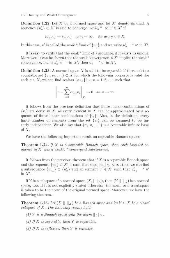
Definition 1.22. Let X be a normed space and let X ′ denote its dual. Asequence u′
n ⊂ X ′ is said to converge weakly * to u′ ∈ X ′ if
〈u′n, v〉 → 〈u′, v〉 as n → ∞, for every v ∈ X.
In this case, u′ is called the weak * limit of u′n and we write u′
n ∗ u′ in X ′.
It is easy to verify that the weak * limit of a sequence, if it exists, is unique.Moreover, it can be shown that the weak convergence in X ′ implies the weak *convergence, i.e., if u′
n u′ in X ′, then u′n ∗ u′ in X ′.
Definition 1.23. A normed space X is said to be separable if there exists acountable set v1, v2, . . . ⊂ X for which the following property is valid: foreach v ∈ X, we can find scalars αn,in
i=1, n = 1, 2, . . ., such that
∥∥∥∥∥v −n∑
i=1
αn,ivi
∥∥∥∥∥X
→ 0 as n → ∞.
It follows from the previous definition that finite linear combinations ofvi are dense in X, as every element in X can be approximated by a se-quence of finite linear combinations of vi. Also, in the definition, everyfinite number of elements from the set vi can be assumed to be lin-early independent. We also say that v1, v2, . . . is a countable infinite basisof X.
We have the following important result on separable Banach spaces.
Theorem 1.24. If X is a separable Banach space, then each bounded se-quence in X ′ has a weakly * convergent subsequence.
It follows from the previous theorem that if X is a separable Banach spaceand the sequence u′
n ⊂ X ′ is such that supn ‖u′n‖X′ < ∞, then we can find
a subsequence u′nk
⊂ u′n and an element u′ ∈ X ′ such that u′
nk∗ u′
in X ′.
If Y is a subspace of a normed space (X, ‖·‖X), then (Y, ‖·‖X) is a normedspace, too. If it is not explicitly stated otherwise, the norm over a subspaceis taken to be the norm of the original normed space. Moreover, we have thefollowing theorem.
Theorem 1.25. Let (X, ‖ · ‖X) be a Banach space and let Y ⊂ X be a closedsubspace of X. The following results hold:
(1) Y is a Banach space with the norm ‖ · ‖X .
(2) If X is separable, then Y is separable.
(3) If X is reflexive, then Y is reflexive.
10 1 Preliminaries
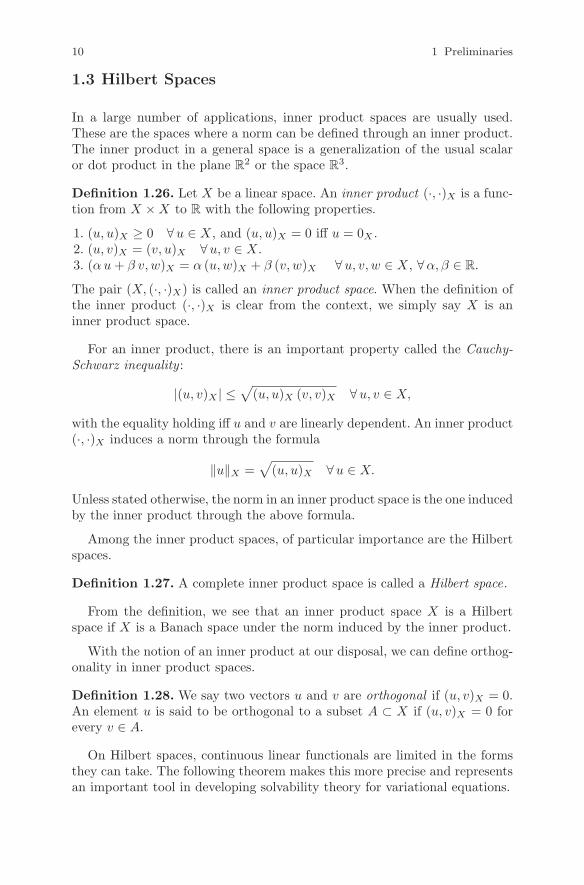
1.3 Hilbert Spaces
In a large number of applications, inner product spaces are usually used.These are the spaces where a norm can be defined through an inner product.The inner product in a general space is a generalization of the usual scalaror dot product in the plane R
2 or the space R3.
Definition 1.26. Let X be a linear space. An inner product (·, ·)X is a func-tion from X × X to R with the following properties.
1. (u, u)X ≥ 0 ∀u ∈ X, and (u, u)X = 0 iff u = 0X .2. (u, v)X = (v, u)X ∀u, v ∈ X.3. (α u + β v, w)X = α (u, w)X + β (v, w)X ∀u, v, w ∈ X, ∀α, β ∈ R.
The pair (X, (·, ·)X) is called an inner product space. When the definition ofthe inner product (·, ·)X is clear from the context, we simply say X is aninner product space.
For an inner product, there is an important property called the Cauchy-Schwarz inequality :
|(u, v)X | ≤√
(u, u)X (v, v)X ∀u, v ∈ X,
with the equality holding iff u and v are linearly dependent. An inner product(·, ·)X induces a norm through the formula
‖u‖X =√
(u, u)X ∀u ∈ X.
Unless stated otherwise, the norm in an inner product space is the one inducedby the inner product through the above formula.
Among the inner product spaces, of particular importance are the Hilbertspaces.
Definition 1.27. A complete inner product space is called a Hilbert space.
From the definition, we see that an inner product space X is a Hilbertspace if X is a Banach space under the norm induced by the inner product.
With the notion of an inner product at our disposal, we can define orthog-onality in inner product spaces.
Definition 1.28. We say two vectors u and v are orthogonal if (u, v)X = 0.An element u is said to be orthogonal to a subset A ⊂ X if (u, v)X = 0 forevery v ∈ A.
On Hilbert spaces, continuous linear functionals are limited in the formsthey can take. The following theorem makes this more precise and representsan important tool in developing solvability theory for variational equations.
1.3 Hilbert Spaces 11
Theorem 1.29. (The Riesz Representation Theorem) Let X be a Hilbertspace and let ℓ ∈ X ′. Then there is a unique u ∈ X such that
ℓ(v) = (u, v)X ∀ v ∈ X.
Moreover,
‖ℓ‖X′ = ‖u‖X .
By the Riesz representation theorem, we may identify a Hilbert spacewith its dual. Consequently, a Hilbert space can also be identified with itsbidual. Therefore, every Hilbert space is reflexive. Combining this result withTheorem 1.21, we see that each bounded sequence in a Hilbert space has aweakly convergent subsequence.
An important class of nonlinear operators defined in a Hilbert space isprovided by the following result.
Theorem 1.30. (The Projection Theorem) Let K be a nonempty closedconvex subset in a Hilbert space X. Then for each u ∈ X, there is a uniqueelement u0 = PKu ∈ K such that
‖u − u0‖X = minv∈K
‖u − v‖X .
The operator PK : X → K is called the projection operator onto K. Theelement u0 = PKu ∈ K is called the projection of u on K and is characterizedby the inequality
(u0 − u, v − u0)X ≥ 0 ∀ v ∈ K. (1.3)
Using inequality (1.3), it is easy to verify that the projection operator isnonexpansive, that is
‖PKu − PKv‖X ≤ ‖u − v‖X ∀u, v ∈ X,
and monotone,
(PKu − PKv, u − v)X ≥ 0 ∀u, v ∈ X.
Moreover, if K is a closed subspace of X, then the operator PK : X → K islinear, and the element u0 = PKu is the unique element of K that satisfies
(u0 − u, v)X = 0 ∀ v ∈ K.
We conclude that u − u0 is, in this case, orthogonal to K.
Let now (X, (·, ·)X) and (Y, (·, ·)Y ) be two Hilbert spaces and denote by‖ · ‖X and ‖ · ‖Y the associated norms. In Section 4.4 of the book, we shalluse the product space
X × Y = z = (x, y) |x ∈ X, y ∈ Y

12 1 Preliminaries
together with the canonical inner product
(z1, z2)X×Y = (x1, x2)X + (y1, y2)Y
for all z1 = (x1, y1), z2 = (x2, y2) ∈ X ×Y . It is easy to verify that (X ×Y,(·, ·)X×Y ) is a Hilbert space and, moreover,
‖z‖2X×Y = ‖x‖2
X + ‖y‖2Y ∀ z = (x, y) ∈ X × Y.
1.4 Miscellaneous Results
Convex functions. We start with some results on convex functions definedon inner product spaces. Let (X, (·, ·)X) be such a space and let ϕ be afunction on X with values in (−∞,∞], i.e., ϕ : X → (−∞,∞]. Below, weadopt the convention that ∞+∞ = ∞ and an expression of the form ∞−∞is undefined. The effective domain of ϕ is the set
D(ϕ) = u ∈ X : ϕ(u) < ∞,
and we say that the function ϕ is proper if D(ϕ) = ∅, that is, there existsu ∈ X such that ϕ(u) < ∞.
Definition 1.31. The function ϕ : X → (−∞,∞] is convex if
ϕ((1 − t)u + tv) ≤ (1 − t)ϕ(u) + tϕ(v) (1.4)
for all u, v ∈ X and t ∈ [0, 1]. The function ϕ is strictly convex if the inequalityin (1.4) is strict for u = v and t ∈ (0, 1).
We note that if ϕ, ψ : X → (−∞,∞] are convex and λ ≥ 0, then thefunctions ϕ + ψ, λϕ and sup ϕ, ψ are also convex.
Definition 1.32. The function ϕ : X → (−∞,∞] is said to be lower semi-continuous (l.s.c.) at u ∈ X if
lim infn→∞
ϕ(un) ≥ ϕ(u) (1.5)
for each sequence un ⊂ X converging to u in X. The function ϕ is l.s.c. if itis l.s.c. at every point u ∈ X. When inequality (1.5) holds for each sequenceun ⊂ X that converges weakly to u, the function ϕ is said to be weaklylower semicontinuous at u. The function ϕ is weakly l.s.c. if it is weakly l.s.c.at every point u ∈ X.
It is easy to see that the norm function u → ‖u‖X = (u, u)12
X is weaklylower semicontinuous. Indeed, let un ⊂ X be such that un u ∈ X. For afixed v ∈ X, the mapping u → (v, u)X defines a linear continuous functional

1.4 Miscellaneous Results 13
on X and therefore
‖u‖2X = (u, u)X = lim
n→∞(u, un)X ≤ ‖u‖X lim inf
n→∞‖un‖X
which implies that
lim infn→∞
‖un‖X ≥ ‖u‖X .
If ϕ is a continuous function then it is also l.s.c. The converse is nottrue, and a lower semicontinuous function can be discontinuous. Since strongconvergence in X implies weak convergence, it follows that a weakly lowersemicontinuous function is lower semicontinuous. Moreover, it can be shownthat a proper convex function ϕ : X → (−∞,∞] is lower semicontinuous ifand only if it is weakly lower semicontinuous.
Let K ⊂ X and consider the function ψK : X → (−∞,∞] defined by
ψK(v) =
0 if v ∈ K,∞ if v ∈ K.
(1.6)
The function ψK is called the indicator function of the set K. It can beproved that the set K is a non-empty closed convex set of X if and only ifits indicator function ψK is a proper convex lower semicontinuous function.
A second example of convex lower semicontinuous function is provided bythe following result, which will be used repeatedly in the following chaptersof this book.
Proposition 1.33. Let (X, (·, ·)X) be an inner product space and let a : X ×X → R be a bilinear symmetric continuous and X-elliptic form. Then thefunction v → a(v, v) is convex and lower semicontinuous.
Proof. The convexity is straightforward to show. To prove the lower semi-continuity, consider a sequence un ⊂ X such that un u ∈ X. Sincea(un − u, un − u) ≥ 0, it follows that
a(un, un) ≥ a(u, un) + a(un, u) − a(u, u) ∀n ∈ N. (1.7)
For a fixed v ∈ X, the mappings u → a(v, u)X and u → a(u, v)X define linearcontinuous functionals on X and therefore
limn→∞
a(u, un) = limn→∞
a(un, u) = a(u, u). (1.8)
We pass to the lower limit in (1.7) and use (1.8) to see that
lim infn→∞
a(un, un) ≥ a(u, u),
which concludes the proof. ⊓⊔

14 1 Preliminaries
By a consequence of the Hahn-Banach theorem, we have the followingproperty of convex lower semicontinuous functions.
Proposition 1.34. Let (X, (·, ·)X) be an inner product space and let ϕ :X → (−∞,∞] be a proper convex lower semicontinuous function. Then ϕ isbounded from below by an affine function, i.e., there exists α ∈ X and β ∈ R
such that ϕ(u) ≥ (α, u)X + β for all u ∈ X.
We now recall the definition of Gateaux differentiable functions.
Definition 1.35. Let ϕ : X → R and let u ∈ X. Then ϕ is Gateaux differ-entiable at u if there exists an element ∇ϕ(u) ∈ X such that
limt→0
ϕ(u + t v) − ϕ(u)
t= (∇ϕ(u), v)X ∀ v ∈ X. (1.9)
The element ∇ϕ(u) that satisfies (1.9) is unique and is called the gradientof ϕ at u. The function ϕ : X → R is said to be Gateaux differentiable ifit is Gateaux differentiable at every point of X. In this case, the operator∇ϕ : X → X that maps every element u ∈ X into the element ∇ϕ(u) iscalled the gradient operator of ϕ.
The convexity of Gateaux differentiable functions can be characterized asfollows.
Proposition 1.36. Let ϕ : X → R be a Gateaux differentiable function.Then ϕ is convex if and only if
ϕ(v) − ϕ(u) ≥ (∇ϕ(u), v − u)X ∀u, v ∈ X. (1.10)
Proof. If ϕ is a convex function, then for all u, v ∈ X and t ∈ (0, 1), from(1.4) we deduce that
t(ϕ(v) − ϕ(u)) ≥ ϕ(u + t(v − u)) − ϕ(u).
We divide both sides of the inequality by t, pass to the limit as t → 0+,and use (1.9) to obtain (1.10). Conversely, assume that (1.10) holds and letu, v ∈ X, t ∈ [0, 1]. Let w = (1 − t)u + tv; it follows from (1.10) that
ϕ(v) − ϕ(w) ≥ (∇ϕ(w), v − w)X ,
ϕ(u) − ϕ(w) ≥ (∇ϕ(w), u − w)X .
We multiply the inequalities above by t and (1 − t), respectively, then addthe results to obtain (1.4), which shows that ϕ is a convex function. ⊓⊔
From the previous proposition, we easily deduce the following result.
Corollary 1.37. Let ϕ : X → R be a convex Gateaux differentiable function.Then ϕ is lower semicontinuous.
1.4 Miscellaneous Results 15
Proof. Let un be a sequence of elements of X converging to u in X. Itfollows from Proposition 1.36 that
ϕ(un) − ϕ(u) ≥ (∇ϕ(u), un − u)X ∀n ∈ N.
We pass to the lower limit as n → ∞ in the previous inequality to obtain(1.5), which concludes the proof. ⊓⊔
Inequality (1.10) suggests a generalization of the gradient operator forconvex functions defined on inner product spaces.
Definition 1.38. Let ϕ : X → (−∞,∞] and let u ∈ X. Then the subdiffer-ential of ϕ at u is the set
∂ϕ(u) = f ∈ X : ϕ(v) − ϕ(u) ≥ (f, v − u)X ∀ v ∈ X . (1.11)
Denote
D(∂ϕ) = u ∈ X : ∂ϕ(u) = ∅ .
A function ϕ is said to be subdifferentiable at u ∈ X if u ∈ D(∂ϕ), and eachelement f ∈ ∂ϕ(u) is called a subgradient of ϕ at u. A function ϕ is saidto be subdifferentiable if it is subdifferentiable at each point u ∈ X, i.e., ifD(∂ϕ) = X.
Using arguments similar to those used in the proof of Corollary 1.37, itcan be shown that a subdifferentiable function ϕ : X → (−∞,∞] is convexand lower semicontinuous. Also, for convex functions, the link between thegradient operator and subdifferential is given by the following result.
Proposition 1.39. Let ϕ : X → R be a convex Gateaux differentiable func-tion. Then ϕ is subdifferentiable, ∂ϕ is a single-valued operator on X, and∂ϕ(u) = ∇ϕ(u) for every u ∈ X.
Proof. Let u ∈ X. From Proposition 1.36 and (1.11) we get ∇ϕ(u) ∈ ∂ϕ(u),which shows that ϕ is subdifferentiable at u. Let f ∈ ∂ϕ(u); using (1.11)we have
ϕ(u + tv) − ϕ(u) ≥ (f, tv)X ∀ v ∈ X, t ∈ R.
Dividing this inequality by t > 0 and using (1.9) we obtain (∇ϕ(u), v)X ≥(f, v)X for all v ∈ X, which shows that f = ∇ϕ(u). Therefore, we obtainthat ∂ϕ(u) = ∇ϕ(u), which concludes the proof. ⊓⊔
The notion of the subdifferential is useful in describing constraints in manybranches of engineering and in mechanics, including those arising in contactproblems, as it will be shown in Section 7.5.
Fixed point theorems. We continue with fixed point results that will beused later in this book.

16 1 Preliminaries
Theorem 1.40. (The Banach Fixed Point Theorem) Let K be a nonemptyclosed subset of a Banach space (X, ‖ · ‖X). Assume that Λ : K → K is acontraction, i.e., there exists a constant α ∈ [0, 1) such that
‖Λu − Λv‖X ≤ α ‖u − v‖X ∀u, v ∈ K.
Then there exists a unique u ∈ K such that Λu = u.
A solution u ∈ K of the operator equation Λu = u is called a fixed point ofΛ in K. We also need a variant of the Banach fixed point theorem, which werecall next. To this end, for an operator Λ, we define its powers inductivelyby the formula Λm = Λ(Λm−1) for m ≥ 2.
Theorem 1.41. Assume that K is a nonempty closed set in a Banach spaceX and let Λ : K → K. Assume also that Λm : K → K is a contraction forsome positive integer m. Then Λ has a unique fixed-point in K.
We now provide a result that will be used repeatedly in Part II of the bookto prove existence results for the solutions of variational inequalities.
Let (X, ‖ · ‖X) be a Banach space, T > 0, and denote by C([0, T ];X) thespace of continuous functions defined on [0, T ] with values in X. It is wellknown that C([0, T ];X) is a Banach space with the norm
‖v‖C([0,T ];X) = maxt∈[0,T ]
‖v(t)‖X .
Lemma 1.42. Let Λ : C([0, T ];X) → C([0, T ];X) be an operator that satis-fies the following property: there exists c > 0 such that
‖Λη1(t) − Λη2(t)‖X ≤ c
∫ t
0
‖η1(s) − η2(s)‖X ds
∀ η1, η2 ∈ C([0, T ];X), t ∈ [0, T ]. (1.12)
Then, there exists a unique element η∗ ∈ C([0, T ];X) such that Λη∗ = η∗.
Proof. A first proof of the lemma can be obtained as follows. Let η1, η2 ∈C([0, T ];X) and let t ∈ [0, T ]. Reiterating (1.12), it follows that
‖Λmη1(t) − Λmη2(t)‖X ≤ cm
∫ t
0
∫ s
0
. . .
∫ u
0︸ ︷︷ ︸m integrals
‖η1(r) − η2(r)‖X dr . . . ds,
which implies that
‖Λmη1 − Λmη2‖C([0,T ];X) ≤ cmTm
m!‖η1 − η2‖C([0,T ];X). (1.13)

1.4 Miscellaneous Results 17
Since
limm→∞
cmTm
m!= 0,
it follows that there exists a positive integer m such that cmT m
m! < 1 and, there-fore, (1.13) shows that Λm is a contraction on the Banach space C([0, T ];X).Lemma 1.42 is now a consequence of Theorem 1.41.
A second proof of the lemma, which avoids the use of Theorem 1.41, is thefollowing: denote
‖η‖β = maxt∈[0,T ]
e−βt ‖η(t)‖X ∀ η ∈ C([0, T ];X),
with β > 0 to be chosen later. Clearly, ‖ · ‖β defines a norm on the spaceC([0, T ];X) that is equivalent to the standard norm ‖ · ‖C([0,T ];X). Using(1.12), after some calculus we find that
‖Λη1 − Λη‖β ≤ c
β‖η1 − η2‖β ∀ η1, η2 ∈ C([0, T ];X).
So, if we choose β such that β > c, then the operator Λ is a contractionon the space C([0, T ];X) endowed with the equivalent norm ‖ · ‖β . By theBanach fixed point theorem (Theorem 1.40), it follows that Λ has a uniquefixed point η∗ ∈ C([0, T ];X), which concludes the proof. ⊓⊔
We continue with the following fixed point result.
Theorem 1.43. (Schauder-Tychonoff) Let X be a reflexive separable Banachspace and let K be a nonempty closed bounded convex subset of X. Let also Λ :K → K be a weakly sequentially continuous map, that is, for each sequencexn ⊂ K, xn x in X =⇒ Λxn Λx in X. Then, there exists an elementx ∈ K such that Λx = x.
Some elementary inequalities. We introduce now some elementary ineq-ualities that will be used in later chapters. To this end, we use below thenotation C([a, b]) for the space of real valued continuous functions defined onthe interval [a, b] ⊂ R.
The following Gronwall inequality will be used frequently in the study ofevolutionary variational inequalities.
Lemma 1.44. (Gronwall’s Inequality) Assume f, g ∈ C([a, b]) satisfying
f(t) ≤ g(t) + c
∫ t
a
f(s) ds ∀ t ∈ [a, b], (1.14)
where c > 0 is a constant. Then
f(t) ≤ g(t) + c
∫ t
a
g(s) ec (t−s) ds ∀ t ∈ [a, b]. (1.15)

18 1 Preliminaries
Moreover, if g is nondecreasing, then
f(t) ≤ g(t) ec (t−a) ∀ t ∈ [a, b]. (1.16)
Proof. Define
F (s) =
∫ s
a
f(r) dr ∀ s ∈ [a, b]. (1.17)
Then F ′(s) = f(s). From assumption (1.14) we get
F ′(s) ≤ g(s) + c F (s) ∀ s ∈ [a, b].
Thus,
(e−c sF (s)
)′ ≤ g(s) e−c s ∀ s ∈ [a, b].
Let t ∈ [a, b]. We integrate this inequality from a to t and note that F (a) = 0;as a result we find
e−c tF (t) ≤∫ t
a
g(s) e−c sds.
So,
F (t) ≤∫ t
a
g(s) ec (t−s)ds. (1.18)
We combine now (1.14) with (1.17) to find that f(t) ≤ g(t) + cF (t), then,using (1.18), we obtain (1.15).
If g is nondecreasing, then (1.15) implies that
f(t) ≤ g(t) + g(t) c
∫ t
a
ec (t−s) ds = g(t) ec (t−a),
which concludes the proof. ⊓⊔
We also need the following result.
Lemma 1.45. (Young’s Inequality) Let p, q ∈ R be two conjugate exponents,that is 1 < p < ∞ and 1
p + 1q = 1. Then
ab ≤ ap
p+
bq
q∀ a, b ≥ 0. (1.19)
Proof. Let a, b ≥ 0. Since (1.19) is obvious in the case a = 0 or b = 0,we assume in what follows that a > 0 and b > 0. Consider the function

1.4 Miscellaneous Results 19
f : (0,∞) → R given by
f(t) = t1p − 1
pt.
We have
f ′(t) =1
p
(t
1p
−1 − 1), f ′′(t) =
1
p
(1
p− 1
)t
1p
−2
and, since p > 1, it follows that the second derivative f ′′ is negative on(0,∞) and therefore the first derivative f ′ is a decreasing function. Equalityf ′(1) = 0 implies that f ′ is positive on (0, 1) and negative on (1,∞), whichshows that f has a global maximum at t = 1. We conclude that f(t) ≤ f(1)for all t ≥ 0, which implies that
t1p − 1 ≤ 1
p(t − 1) ∀ t > 0. (1.20)
We take t = ap
bq in (1.20) and, after some elementary manipulation, using theidentity 1
p + 1q = 1 we obtain (1.19). ⊓⊔
Lemma 1.45 allows us to obtain the following result.
Lemma 1.46. Let p > 0. Then
|u|p−1u(v − u) ≤ 1
p + 1|v|p+1 − 1
p + 1|u|p+1 ∀u, v ∈ R, u = 0. (1.21)
Proof. Let u, v ∈ R, u = 0. It is easy to see that
|u|p−1u(v − u) ≤ |u|p|v| − |u|p+1. (1.22)
Next, applying (1.19) with a = |v|, b = |u|p and with the pair of conjugateexponents (p + 1, p+1
p ), we have
|u|p|v| ≤ 1
p + 1|v|p+1 +
p
p + 1|u|p+1. (1.23)
Inequality (1.21) is now a consequence of (1.22) and (1.23). ⊓⊔

Chapter 2
Function Spaces
We introduce in this chapter the function spaces that will be relevant tothe subsequent developments in this monograph. The function spaces to bediscussed include spaces of continuous and continuously differentiable func-tions, Lebegue and Sobolev spaces, associated with an open bounded domainΩ ⊂ R
d. In order to treat time-dependent problems, we also introduce spacesof vector-valued functions, i.e., spaces of mappings defined on a time interval[0, T ] ⊂ R with values into a Banach or Hilbert space X.
2.1 The Spaces Cm(Ω) and Lp(Ω)
Let Ω be an open bounded subset of Rd, where d is a positive integer. We
denote by Γ the boundary of Ω, and Ω = Ω ∪ Γ the closure of Ω. A typ-ical point in R
d is denoted by x = (x1, . . . , xd) or x = (x1, . . . , xd)T . It is
convenient to use the multi-index notation for partial derivatives. An orderedcollection of d non-negative integers, α = (α1, . . . , αd), is called a multi-index.
The quantity |α| =∑d
i=1 αi is said to be the length of α. If v is an m-timesdifferentiable function, then for each α with |α| ≤ m,
Dαv(x) =∂|α|v(x)
∂xα1
1 · · · ∂xαd
d
is the αth partial derivative. This is a handy notation for partial derivatives.Some examples are
∂1v =∂v
∂x1= Dαv, α = (1, 0, . . . , 0),
∂dv
∂x1 · · · ∂xd= Dαv, α = (1, 1, . . . , 1).
21
22 2 Function Spaces
The set of all the partial derivatives of order m of a function v can be expr-essed as Dαv : |α| = m . There are other notations commonly used forpartial derivatives; e.g., the partial derivative ∂v/∂xi is also written as ∂xi
v,or ∂iv, or vxi
, or v,i.
The spaces Cm(Ω). Let C(Ω) be the space of functions that are uniformlycontinuous on Ω. Each function in C(Ω) is bounded. The notation C(Ω) isconsistent with the fact that a uniformly continuous function on Ω has aunique continuous extension to Ω. For v ∈ C(Ω), we always understand itsboundary values on Γ to be the continuous extension of the values of v in Ω.The space C(Ω) is a Banach space with the norm
‖v‖C(Ω) = sup |v(x)| : x ∈ Ω ≡ max |v(x)| : x ∈ Ω .
Denote Z+ the set of non-negative integers. For every m ∈ Z+, Cm(Ω) isthe space of functions that, together with their derivatives of order less thanor equal to m, are continuous up to the boundary,
Cm(Ω) = v ∈ C(Ω) : Dαv ∈ C(Ω) for |α| ≤ m .
When m = 0, we usually write C(Ω) instead of C0(Ω). The space Cm(Ω) isa Banach space with the norm
‖v‖Cm(Ω) =∑
|α|≤m
‖Dαv‖C(Ω).
We also set
C∞(Ω) =
∞⋂
m=0
Cm(Ω) ≡ v ∈ C(Ω) : v ∈ Cm(Ω) ∀m ∈ Z+ ,
the space of infinitely differentiable functions.Given a function v : Ω → R, its support is defined to be
supp v = x ∈ Ω : v(x) = 0 .
We say that v has a compact support if supp v is a proper subset of Ω:supp v ⊂ Ω. Thus, if v has a compact support, then there is a neighboringopen strip about the boundary Γ such that v is zero on the part of the stripthat lies inside Ω. Later on, we will need the space
C∞0 (Ω) = v ∈ C∞(Ω) : supp v ⊂ Ω .
Obviously, C∞0 (Ω) ⊂ C∞(Ω).
The spaces Lp(Ω). For every number p ∈ [1,∞) we denote by Lp(Ω) thelinear space of (equivalence classes of) measurable functions v : Ω → R

2.1 The Spaces Cm(Ω) and Lp(Ω) 23
for which
‖v‖Lp(Ω) =
(∫
Ω
|v(x)|pdx
)1/p
< ∞, (2.1)
where the integration is understood to be in the sense of Lebesgue. The map-ping v → ‖v‖Lp(Ω) is a norm on Lp(Ω). Here and below, it is understood thatv represents an equivalence class of functions, two functions being equivalentif they are equal almost everywhere (a.e.), that is, equal except on a subsetof Ω of Lebesgue measure zero.
The definition of the spaces Lp(Ω) can be extended to include the casep = ∞ in the following manner. For every measurable function v : Ω → R
denote
‖v‖L∞(Ω) = ess supx∈Ω
|v(x)|
= inf M ∈ [0,∞] : |v(x)| ≤ M a.e. x ∈ Ω . (2.2)
The quantity (2.2) is called the essential supremum of |v|, and we say thatv is essentially bounded if ‖v‖L∞(Ω) < ∞. We denote by L∞(Ω) the linearspace of (equivalence classes of) measurable functions v : Ω → R that areessentially bounded. The mapping v → ‖v‖L∞(Ω) is a norm on the spaceL∞(Ω).
For p ∈ [1,∞], its conjugate exponent q ∈ [1,∞] is defined by the relations
1
p+
1
q= 1 if p = 1,
q = ∞ if p = 1.
Here, we adopt the convention 1/∞ = 0 and therefore q = 1 if p = ∞.
Some basic properties of the Lp spaces are summarized below.
Theorem 2.1. Let Ω be an open bounded set in Rd and let p ∈ [1,∞]. Then:
(a) Lp(Ω) is a Banach space.(b) Every Cauchy sequence in Lp(Ω) has a subsequence that converges point-
wise a.e. on Ω.(c) (Holder’s inequality) Let u ∈ Lp(Ω), v ∈ Lq(Ω). Then
∫
Ω
|u(x) v(x)| dx ≤ ‖u‖Lp(Ω)‖v‖Lq(Ω).
(d) For 1 ≤ p < ∞, the dual (Lp(Ω))′ of Lp(Ω) is the space Lq(Ω). Moreover,if p ∈ (1,∞), the space Lp(Ω) is reflexive.
(e) For 1 ≤ p < ∞, Lp(Ω) is a separable space.
The case p = 2 is special since in this case p = q = 2. A simple consequenceof the last theorem is the following result.

24 2 Function Spaces
Corollary 2.2. The space L2(Ω) is a Hilbert space with the inner product
(u, v)L2(Ω) =
∫
Ω
u(x) v(x) dx ∀u, v ∈ L2(Ω).
Moreover, L2(Ω) is separable and the following Cauchy-Schwarz inequalityholds:
∣∣∣∣∫
Ω
u(x) v(x) dx
∣∣∣∣ ≤ ‖u‖L2(Ω)‖v‖L2(Ω) ∀u, v ∈ L2(Ω).
We now introduce the spaces of locally integrable functions that will beused in the next section in order to introduce the weak derivatives of real-valued functions defined on Ω.
Definition 2.3. Let 1 ≤ p < ∞. A function v : Ω ⊂ Rd → R is said to
be locally p-integrable, v ∈ Lploc(Ω), if for every x ∈ Ω, there is an open
neighborhood Ω′ of x such that Ω′ ⊂⊂ Ω (i.e., Ω′ ⊂ Ω) and v ∈ Lp(Ω′).
We have the following useful result ([153, p. 18]).
Lemma 2.4. (Generalized Variational Lemma) Let v ∈ L1loc(Ω) with Ω a
nonempty open set in Rd. If
∫
Ω
v(x) φ(x) dx = 0 ∀φ ∈ C∞0 (Ω),
then v = 0 a.e. on Ω.
In Section 2.3, we shall need the space
L2(Ω)d = u = (ui) : ui ∈ L2(Ω), i = 1, . . . , d . (2.3)
This is a Hilbert space with the canonical inner product
(u,v)L2(Ω)d =
d∑
i=1
∫
Ω
ui(x)vi(x) dx
and the associated norm
‖u‖L2(Ω)d =
( d∑
i=1
∫
Ω
u2i (x) dx
) 12
.
2.2 Sobolev Spaces
Sobolev spaces are indispensable tools in the study of boundary value prob-lems. To introduce Sobolev spaces, we first need to extend the definition of

2.2 Sobolev Spaces 25
derivatives. The starting point is the classical “integration by parts” formula
∫
Ω
v(x) Dαφ(x) dx = (−1)|α|∫
Ω
Dαv(x) φ(x) dx, (2.4)
which holds for v ∈ Ck(Ω), φ ∈ C∞0 (Ω) and |α| ≤ k. This formula, relating
differentiation and integration, is the most important formula in calculus. Theweak derivative is an extension of the classical derivative, i.e., if the classicalderivative exists, then the two derivatives coincide. To ensure that the weakderivative is useful, we require that the integration by parts formula (2.4)holds. A more general approach for the extension of the classical derivativesis to first introduce the derivatives in the distributional sense. A detaileddiscussion of distributions and the derivatives in the distributional sense canbe found in several monographs, e.g., [138]. Here we choose to introduce theconcept of the weak derivatives directly, which is sufficient for this work.
Definition 2.5. Let Ω be a nonempty open set in Rd, v, w ∈ L1
loc(Ω). Thenw is called an αth weak derivative of v if
∫
Ω
v(x) Dαφ(x) dx = (−1)|α|∫
Ω
w(x) φ(x) dx ∀φ ∈ C∞0 (Ω). (2.5)
Applying Lemma 2.4, we see that when a weak derivative exists, it isuniquely defined up to a set of measure zero. Also, from the definition of theweak derivative, we see that if v is k-times continuously differentiable on Ω,then, for each α with |α| ≤ k, the classical partial derivative Dαv is also theαth weak derivative of v. For this reason, we use the notation Dαv also forthe αth weak derivative of v and we note that Dαv = v if |α| = 0.
We continue with the following definition.
Definition 2.6. Let k be a non-negative integer, k ∈ Z+, and let p ∈ [1,∞].The Sobolev space W k,p(Ω) is the set of all the functions v ∈ L1
loc(Ω) suchthat for each multi-index α with |α| ≤ k, the αth weak derivative Dαv existsand belongs to Lp(Ω). The norm in the space W k,p(Ω) is defined as
‖v‖W k,p(Ω) =
(∑
|α|≤k
‖Dαv‖pLp(Ω)
)1/p
if 1 ≤ p < ∞,
max|α|≤k
‖Dαv‖L∞(Ω) if p = ∞.
We note that W 0,p(Ω) = Lp(Ω), and when p = 2, we write W k,2(Ω) ≡Hk(Ω).
A seminorm over the space W k,p(Ω) is
|v|W k,p(Ω) =
(∑
|α|=k
‖Dαv‖pLp(Ω)
)1/p
if 1 ≤ p < ∞,
max|α|=k
‖Dαv‖L∞(Ω) if p = ∞.

26 2 Function Spaces
It is not difficult to see that W k,p(Ω) is a normed space. Moreover, wehave the following results, which summarize the basic properties of Sobolevspaces.
Theorem 2.7. Let Ω be an open bounded set in Rd, k ∈ Z+ and p ∈ [1,∞].
Then:
(a) W k,p(Ω) is a Banach space.(b) W k,p(Ω) is reflexive if 1 < p < ∞.(c) W k,p(Ω) is separable if 1 ≤ p < ∞.
A simple consequence of the Theorem 2.7 combined with Corollary 2.2 isthe following result.
Corollary 2.8. The Sobolev space Hk(Ω) is a separable Hilbert space withthe inner product
(u, v)Hk(Ω) =
∫
Ω
∑
|α|≤k
Dαu(x) Dαv(x) dx ∀u, v ∈ Hk(Ω).
The closure of the space C∞0 (Ω) with respect to the norm ‖·‖W k,p(Ω) gives
a closed subspace of W k,p(Ω), denoted W k,p0 (Ω). When p = 2, we use the
notation Hk0 (Ω) ≡ W k,2
0 (Ω). It follows from Theorem 2.7 and Corollary 2.8
that W k,p0 (Ω) is a Banach space and Hk
0 (Ω) is a Hilbert space. It can be
shown that the seminorm | · |W k,p(Ω) is a norm on W k,p0 (Ω) and there exists
a constant c > 0 such that
|v|W k,p(Ω) ≤ ‖v‖W k,p(Ω) ≤ c |v|W k,p(Ω) ∀ v ∈ W k,p0 (Ω).
We now collect some important properties of Sobolev spaces. Some of themrequire a certain degree of regularity on the boundary Γ of the domain Ωand, for this reason, we introduce the following definition.
Definition 2.9. Let Ω be open and bounded in Rd. We say that Ω has a
Lipschitz continuous boundary Γ if for each point x0 ∈ Γ there exists r > 0and a Lipschitz continuous function g : R
d−1 → R such that, upon relabelingthe coordinate axes if necessary, we have
Ω ∩ B(x0, r) = x ∈ B(x0, r) : xd > g(x1, . . . , xd−1) .
Here, B(x0, r) denotes the ball of Rd centered at x0 with radius r. Also,
we recall that a real-valued function g : Rd−1 → R is said to be Lipschitz
continuous if for some constant Lg, there holds the inequality
|g(x) − g(y)| ≤ Lg ‖x − y‖ ∀x,y ∈ Rd−1,

2.2 Sobolev Spaces 27
where ‖x − y‖ denotes the standard Euclidean distance between x and y,
‖x − y‖ =
(d−1∑
i=1
|xi − yi|2)1/2
.
We note that, since Γ is a compact set in Rd, in Definition 2.9 we can
actually find a finite number of points xiNi=1 on the boundary, positive
numbers riNi=1 and Lipschitz continuous functions giN
i=1, such that Γ iscovered by the union of the balls B(xi, ri), 1 ≤ i ≤ N , and
Ω ∩ B(xi, ri) = x ∈ B(xi, ri) : xd > gi(x1, . . . , xd−1)
upon relabeling the coordinate axes, if necessary.With a slight abuse of terminology, we say that a domain Ω is a Lipschitz
domain if it is an open bounded domain with Lipschitz continuous boundary.In the following, we always assume that Ω is a Lipschitz domain, and we notethat this assumption is, in fact, not needed for some of the results statedbelow.
We have the following result on the approximation of Sobolev functionsby smooth functions.
Theorem 2.10. Assume that Ω ⊂ Rd is a Lipschitz domain, k ∈ Z+ and p ∈
[1,∞). Then for each v ∈ W k,p(Ω), there exists a sequence vn ⊂ C∞(Ω)such that
‖vn − v‖W k,p(Ω) → 0 as n → ∞.
From the definition of the space W k,p0 (Ω), we immediately obtain the
following density result.
Theorem 2.11. Under the assumptions of Theorem 2.10, for every v ∈W k,p
0 (Ω), there exists a sequence vn ⊂ C∞0 (Ω) such that
‖vn − v‖W k,p(Ω) → 0 as n → ∞.
To compare Sobolev spaces with different indices, we need the followingdefinitions.
Definition 2.12. Let X and Y be two normed spaces with X ⊂ Y . We saythe space X is continuously embedded in Y and write X → Y , if the identityoperator I : X → Y is continuous. We say the space X is compactly embeddedin Y and write X →→ Y , if the identity operator I : X → Y is compact.
It is easy to see that X → Y if and only if there exists c > 0 such that
‖v‖Y ≤ c ‖v‖X ∀ v ∈ X (2.6)

28 2 Function Spaces
or, equivalently,
∀ vn ⊂ X, vn → v in X =⇒ vn → v in Y.
Also, it can be proved that X →→ Y iff
∀ vn ⊂ X, vn v in X =⇒ vn → v in Y.
Some properties regarding embeddings and compact embeddings involv-ing Sobolev spaces, which are important in analyzing the regularity of weaksolutions of boundary value problems, are summarized in the followingtheorem.
Theorem 2.13. Let Ω ⊂ Rd be a Lipschitz domain, k ∈ Z+ and p ∈ [1,∞).
Then the following statements are valid.(a) If k < d
p , then W k,p(Ω) → Lq(Ω) for every q ≤ p∗ and W k,p(Ω) →→Lq(Ω) for every q < p∗, where 1
p∗= 1
p − kd .
(b) If k = dp , then W k,p(Ω) →→ Lq(Ω) for every q < ∞.
(c) If k > dp , then W k,p(Ω) →→ Cm(Ω) for every integer m that satisfies
0 ≤ m < k − dp .
A direct consequence of Theorem 2.13 is the following result.
Corollary 2.14. Let Ω ⊂ Rd be a Lipschitz domain, p ∈ [1,∞) and let k be
a positive integer. Then W k,p(Ω) →→ Lp(Ω).
In this work, we shall use the embedding result
H1(Ω) →→ L2(Ω) (2.7)
which is obtained from Corollary 2.14 by taking k = 1 and p = 2.
Sobolev spaces are defined through Lp(Ω) spaces. Hence Sobolev functionsare uniquely defined only a.e. in Ω. Since the boundary Γ has measure zeroin R
d, the boundary values of a Sobolev function seem to be not well defined.Nevertheless, it is possible to define the trace of a Sobolev function on theboundary in such a way that for a Sobolev function that is continuous up tothe boundary, its trace coincides with its boundary value.
Theorem 2.15. Assume that Ω is a Lipschitz domain in Rd with bound-
ary Γ and 1 ≤ p < ∞. Then there exists a linear continuous operatorγ : W 1,p(Ω) → Lp(Γ ) such that γv = v|Γ if v ∈ W 1,p(Ω) ∩ C(Ω). More-over, the mapping γ : W 1,p(Ω) → Lp(Γ ) is compact, i.e., for every boundedsequence vn in W 1,p(Ω), there is a subsequence vnk
⊂ vn such thatγvnk
is convergent in Lp(Γ ).
The operator γ is called the trace operator, and γv can be termed thetrace of v ∈ W 1,p(Ω). For the sake of simplicity, when no ambiguity occurs,
2.3 Equivalent Norms on the Space H1(Ω) 29
we usually write v instead of γv. Note that the continuity of γ implies thatthere exists a constant c > 0, which depends on Ω, such that
‖γv‖Lp(Γ ) ≤ c ‖v‖W 1,p(Ω) ∀ v ∈ W 1,p(Ω). (2.8)
Generally, the trace operator is neither an injection nor a surjectionfrom W 1,p(Ω) to Lp(Γ ) (the only exception is when p = 1, since then thetrace operator is surjective from W 1,1(Ω) to L1(Γ )). When p > 1, the rangeγ(W 1,p(Ω)) is a space smaller than Lp(Γ ).
2.3 Equivalent Norms on the Space H1(Ω)
In studying second-order boundary value problems, the Sobolev space H1(Ω)plays a crucial role. For this reason, since the antiplane contact problems westudy in Part IV of this monograph lead to second-order boundary valueproblems, in this section we pay a particular attention to the Sobolev spaceH1(Ω).
Let Ω be a Lipschitz domain in Rd. Recall that
H1(Ω) = u ∈ L2(Ω) : ∇u ∈ L2(Ω)d
where ∇u = (∂1u, . . . , ∂du) represents the gradient operator. The spaceH1(Ω) is a Hilbert space with the inner product
(u, v)H1(Ω) = (u, v)L2(Ω) + (∇u, ∇v)L2(Ω)d (2.9)
and the associated norm
‖u‖H1(Ω) =(‖u‖2
L2(Ω) + ‖∇u‖2L2(Ω)d
) 12 . (2.10)
A seminorm over the space H1(Ω) is
|u|H1(Ω) = ‖∇u‖L2(Ω)d .
It also follows from Theorem 2.15 that the trace map γ : H1(Ω) → L2(Γ )is a linear continuous and compact operator. In what follows, we simply writev for the trace γv of an element v ∈ H1(Ω) and we note that inequality (2.8)shows that there exists c > 0, which depends on Ω, such that
‖v‖L2(Γ ) ≤ c ‖v‖H1(Ω) ∀ v ∈ H1(Ω). (2.11)
The following result can be used to generate various equivalent norms onH1(Ω).

30 2 Function Spaces
Theorem 2.16. Let Ω be an open, bounded, and connected set in Rd with a
Lipschitz boundary Γ . Assume that p1, p2, . . . , pN are continuous seminormson H1(Ω) with the property that the functional p defined by
p(v) = ‖∇v‖L2(Ω)d +
N∑
j=1
pj(v) ∀ v ∈ H1(Ω) (2.12)
is a norm on H1(Ω). Then p and ‖ · ‖H1(Ω) are equivalent norms on H1(Ω).
Proof. Since p1, p2, . . . , pN are continuous seminorms on H1(Ω) there existpositive constants M1, M2 . . . , MN such that
pj(v) ≤ Mj‖v‖H1(Ω) ∀ v ∈ H1(Ω), j = 1, . . . N
and therefore (2.12) implies that
p(v) ≤ c1 ‖v‖H1(Ω) ∀ v ∈ H1(Ω), (2.13)
where c1 = max 1, M1, . . . , MN > 0.
We shall prove that there exists c2 > 0 such that
p(v) ≥ c2 ‖v‖H1(Ω) ∀ v ∈ H1(Ω). (2.14)
To this end, we argue by contradiction. Suppose that this inequality is false;then, for all n ∈ N there exists vn ∈ H1(Ω) such that
‖vn‖H1(Ω) = 1, (2.15)
p(vn) ≤ 1
n. (2.16)
We combine (2.12) and (2.16) to see that
‖∇vn‖L2(Ω)d +
N∑
j=1
pj(vn) ≤ 1
n∀n ∈ N,
which shows that ∇vn → 0 in L2(Ω)d and pj(vn) → 0 for all j = 1, . . . , N ,as n → ∞. Equality (2.15) shows that vn is a bounded sequence in H1(Ω)and, using the compact embedding (2.7), it follows that there exists a functionv ∈ L2(Ω) and a subsequence of the sequence vn, still denoted by vn,such that vn → v in L2(Ω) as n → ∞. Since
∫
Ω
vn(x) ∂iφ(x) dx = −∫
∂ivn(x) φ(x) dx ∀φ ∈ C∞0 (Ω),

2.3 Equivalent Norms on the Space H1(Ω) 31
vn → v in L2(Ω) and ∂ivn → 0 in L2(Ω) ∀ i = 1, . . . , d, passing to the limitin the previous equality we obtain that
∫
Ω
v(x) ∂iφ(x) dx = 0 ∀φ ∈ C∞0 (Ω) ∀ i = 1, . . . , d.
This last equality shows that v has weak derivatives of first order and thesederivatives vanish a.e. in Ω. We conclude that v ∈ H1(Ω) and ∇v = 0. Itfollows from (2.10) that
‖vn − v‖H1(Ω) =(‖vn − v‖2
L2(Ω) + ‖∇vn‖2L2(Ω)d
) 12
and since vn → v ∈ L2(Ω), ∇vn → 0 in L2(Ω)d, we find that
vn → v in H1(Ω) as n → ∞. (2.17)
Next, since the seminorms p1, . . . , pN are continuous, (2.12) and (2.17) implythat
p(vn) → p(v) as n → ∞
and, therefore, by (2.16) we find that p(v) = 0. Using now the fact that pis a norm on the space H1(Ω), it follows that v = 0, which contradicts theequality ‖v‖H1(Ω) = 1 obtained by combining (2.15) and (2.17). Therefore,inequality (2.14) holds.
It follows that the norm p satisfies (2.13) and (2.14), which concludes theproof. ⊓⊔
Many useful inequalities can be derived as consequence of Theorem 2.16,see [57] and [126] for details. Here, we present only one consequence of thetheorem, which will be used in Section 8.2 of this manuscript.
Corollary 2.17. Let Ω be an open, bounded, and connected set in Rd with
a Lipschitz boundary Γ and let Γ1 be a measurable part of Γ such thatmeas Γ1 > 0. Then the functional p on H1(Ω) defined by
p(v) = ‖∇v‖L2(Ω)d +
∫
Γ1
|v| da ∀ v ∈ H1(Ω) (2.18)
is a norm on H1(Ω), equivalent to the norm ‖ · ‖H1(Ω).
Proof. We apply Theorem 2.16 to the special case N = 1 and
p1(v) =
∫
Γ1
|v| da.
32 2 Function Spaces
Clearly, p1 is a seminorm on the space H1(Ω); moreover, by using the Cauchy-Schwarz inequality and (2.11), we have
p1(v) =
∫
Γ1
|v| da ≤(∫
Γ1
da
) 12(∫
Γ1
v2 da
) 12
≤ (meas Γ1)12 ‖v‖L2(Γ1) ≤ c (meas Γ1)
12 ‖v‖H1(Ω) ∀ v ∈ H1(Ω),
which shows that p1 is continuous. Assume now that p(v) = 0; then ∇v = 0
and∫
Γ1v da = 0; the first equality shows that v is a constant in Ω, v(x) = k
a.e. x ∈ Ω, and the second one shows that
∫
Γ1
k da = k (meas Γ1) = 0,
which implies that k = 0. Thus, v = 0 and therefore p is a norm on H1(Ω).Corollary 2.17 is now a consequence of Theorem 2.16. ⊓⊔
2.4 Spaces of Vector-valued Functions
We shall need the spaces of vector-valued functions in studying time-dependentvariational problems. In the following, if it is not specified otherwise,(X, ‖ · ‖X) will denote a real Banach space and [0, T ] will denote the timeinterval of interest, for T > 0.
Cm([0, T ];X) spaces. We define C([0, T ];X) to be the space of functionsv : [0, T ] → X that are continuous on the closed interval [0, T ]. With thenorm
‖v‖C([0,T ];X) = maxt∈[0,T ]
‖v(t)‖X ,
the space C([0, T ];X) is a Banach space.
Definition 2.18. A function v : [0, T ] → X is said to be (strongly) differ-entiable at t0 ∈ [0, T ] if there exists an element in X, denoted as v′(t0) andcalled the (strong) derivative of v at t0, such that
limh→0
∥∥∥∥1
h(v(t0 + h) − v(t0)) − v′(t0)
∥∥∥∥X
= 0,
where the limit is taken with respect to h with t0 +h ∈ [0, T ]. The derivativeat t0 = 0 is defined as a right-sided limit and that at t0 = T as a left-sidedlimit. The function v is said to be differentiable on [0, T ] if it is differentiableat every t0 ∈ [0, T ]. It is differentiable a.e. if it is differentiable a.e. on (0, T ).In this case, the function v′ is called the (strong) derivative of v. Higher

2.4 Spaces of Vector-valued Functions 33
derivatives v(j), j ≥ 2, are defined recursively by v(j) = (v(j−1))′. Usually weuse the notation v = v′ and we understand v(0) to be v.
For an integer m ≥ 0, we define the space
Cm([0, T ];X) = v ∈ C([0, T ];X) : v(j) ∈ C([0, T ];X), j = 1, . . . , m .
This is a Banach space with the norm
‖v‖Cm([0,T ];X) =
m∑
j=0
maxt∈[0,T ]
‖v(j)(t)‖X .
In particular, C1([0, T ];X) denotes the space of continuously differentiablefunctions on [0, T ] with values in X. This is a Banach space with the norm
‖v‖C1([0,T ];X) = maxt∈[0,T ]
‖v(t)‖X + maxt∈[0,T ]
‖v(t)‖X .
We also set
C∞([0, T ];X) =
∞⋂
m=0
Cm([0, T ];X)
≡ v ∈ C([0, T ];X) : v ∈ Cm([0, T ];X) ∀m ∈ Z+,
the space of infinitely differentiable functions defined on [0, T ] with valuesin X.
The spaces Lp(0, T ;X). For p ∈ [1,∞), we define Lp(0, T ;X) to be the space
of all measurable functions v : [0, T ] → X such that∫ T
0‖v(t)‖p
Xdt < ∞. Withthe norm
‖v‖Lp(0,T ;X) =
(∫ T
0
‖v(t)‖pXdt
)1/p
,
the space Lp(0, T ;X) becomes a Banach space. We define L∞(0, T ;X) to bethe space of all measurable functions v : [0, T ] → X such that t → ‖v(t)‖X isessentially bounded on [0, T ]. The space L∞(0, T ;X) is a Banach space withthe norm
‖v‖L∞(0,T ;X) = ess supt∈[0,T ]
‖v(t)‖X .
When (X, (·, ·)X) is a Hilbert space, L2(0, T ;X) is also a Hilbert space withthe inner product given by
(u, v)L2(0,T ;X) =
∫ T
0
(u(t), v(t))X dt.
Also, below we shall use the notation Lp(0, T ) for the space Lp(0, T ; R).

34 2 Function Spaces
The following theorem summarizes some basic properties of the spacesLp(0, T ;X).
Theorem 2.19. Let p ∈ [1,∞]. Then:
(a) C([0, T ];X) is dense in Lp(0, T ;X) and the embedding is continuous.(b) If X → Y , then Lp(0, T ;X) → Lq(0, T ;Y ) for 1 ≤ q ≤ p ≤ ∞.
The following result of Lebesgue is useful when we localize a global relation.
Theorem 2.20. Assume that v ∈ L1(0, T ;X). Then
limh→0
1
h
∫ t0+h
t0
‖v(t) − v(t0)‖X dt = 0 for almost all t0 ∈ (0, T ).
We see that Theorem 2.20 implies that if v ∈ L1(0, T ;X), then
limh→0
1
h
∫ t0+h
t0
v(t) dt = v(t0) for almost all t0 ∈ (0, T ).
Here the limit is understood in the sense of the norm of X, that is,
limh→0
∥∥∥∥1
h
∫ t0+h
t0
v(t) dt − v(t0)
∥∥∥∥X
= 0 for almost all t0 ∈ (0, T ).
The next result describes the dual of the space Lp(0, T ;X), in the Hilber-tian case.
Theorem 2.21. Let p ∈ [1,∞) and let q ∈ (1,∞] be its conjugate. AssumeX is a Hilbert space. Then the dual of the space Lp(0, T ;X) is Lq(0, T ;X).
The duality pairing between the space Lp(0, T ;X) and its dual is given by
〈u′, u〉 =
∫ T
0
(u′(t), u(t))Xdt.
The spaces W k,p(0, T ;X). To define the Sobolev spaces of vector-valuedfunctions, we need to define in an appropriate way derivatives with respectto the time variable for functions defined on [0, T ] with values in X. Theapproach is similar to that taken in the case of weak derivatives of real-valued functions, see Definition 2.5; that is, we take as a starting point theelementary integration by parts formula
∫ T
0
v(t)φ(m)(t) dt = (−1)m
∫ T
0
v(m)(t)φ(t) dt
which holds for all functions v ∈ Cm([0, T ];X) and φ ∈ C∞0 (0, T ). Here m is
a positive integer and (·)(m) = dm(·)/dtm.

2.4 Spaces of Vector-valued Functions 35
Definition 2.22. A function v : [0, T ] → X is said to be locally integrable,v ∈ L1
loc(0, T ;X), if for every closed interval B ⊂ [0, T ], we have
∫
B
‖v(t)‖Xdt < ∞.
Definition 2.23. Let v, w ∈ L1loc(0, T ;X). Then w is called a mth weak
derivative of v if
∫ T
0
v(t) φ(m)(t) dt = (−1)m
∫ T
0
w(t) φ(t) dt ∀φ ∈ C∞0 (0, T ). (2.19)
It can be proved that when a weak derivative exists, it is unique. For thisreason, if v and w satisfy (2.19) for some positive integer m we write simplyw = v(m). The first two weak derivatives are also denoted by v, v and wenote that v(0) = v.
For k ∈ Z+ and 1 ≤ p ≤ ∞, we introduce the space
W k,p(0, T ;X) = v ∈ Lp(0, T ;X) : ‖v(m)‖Lp(0,T ;X) < ∞ ∀m ≤ k .
When p < ∞, we define the norm in the space W k,p(0, T ;X) by
‖v‖W k,p(0,T ;X) =
(∫ T
0
∑
0≤m≤k
‖v(m)(t)‖pXdt
)1/p
.
When p = ∞, the norm is defined as
‖v‖W k,∞(0,T ;X) = max0≤m≤k
ess supt∈[0,T ]
‖v(m)(t)‖X .
If X is a Hilbert space and p = 2, then the space
Hk(0, T ;X) ≡ W k,2(0, T ;X)
is a Hilbert space with the inner product
(u, v)Hk(0,T ;X) =∑
0≤m≤k
∫ T
0
(u(m)(t), v(m)(t))X dt.
We have the following result.
Theorem 2.24. Assume that X is a Banach space and p ∈ [1,∞]. ThenW 1,p(0, T ;X) → C([0, T ];X).
The previous theorem shows that every element v ∈ W 1,p(0, T ;X) canbe identified with an element, still denoted by v, in the space C([0, T ];X),

36 2 Function Spaces
possibly after a modification on a subset of [0, T ] with zero measure. More-over, there is a positive constant c such that
‖v‖C([0,T ];X) ≤ c ‖v‖W 1,p(0,T ;X) ∀ v ∈ W 1,p(0, T ;X).
The next result can help us to understand the nature of the functions in thespaces W k,p(0, T ;X). For this, we recall the definition of absolute continuity.
Definition 2.25. A function v : [0, T ] → X is absolutely continuous if forany ε > 0, there exists a δ = δ(ε) > 0 such that
∑n ‖v(bn) − v(an)‖X < ε
whenever (an, bn)n ⊂ [0, T ] is a countable family of pairwisely disjointintervals with total length
∑n(bn − an) < δ.
We have the following characterization for the space W k,p(0, T ;X).
Theorem 2.26. Let k > 0 be an integer, p ∈ [1,∞], and v ∈ Lp(0, T ;X).Then v ∈ W k,p(0, T ;X) if and only if v(t) = w(t) a.e. on (0, T ) forsome w ∈ Ck−1([0, T ];X) such that w, w′, . . . , w(k−1) are absolutely con-tinuous on [0, T ], the k-th strong derivative w(k) exists a.e., and w(k) ∈Lp(0, T ;X).
Because of Theorem 2.26, we usually simply say v ∈ W k,p(0, T ;X) iff v,v′, . . . , v(k−1) are absolutely continuous on [0, T ] and v(k) ∈ Lp(0, T ;X).
It is well known that every real-valued absolutely continuous function v :[0, T ] → R is differentiable a.e. on (0, T ) and it can be expressed as theindefinite integral of its derivative. Some simple examples (see for instance [11,p. 15]) show that this fails when v is absolutely continuous from [0, T ] to ageneral Banach space X. However, the following theorem, obtained in [92],holds.
Theorem 2.27. Let X be a reflexive Banach space and let v : [0, T ] → X bean absolutely continuous function. Then v is a.e. differentiable on (0, T ), itsderivative v belongs to L1(0, T ;X), and
v(t) = v(0) +
∫ t
0
v(s) ds ∀ t ∈ [0, T ]. (2.20)
Using Theorems 2.26 and 2.27, we can show the following results, whichwill be used on several occasions in the rest of the manuscript.
Proposition 2.28. Let X be a reflexive Banach space and let v : [0, T ] → X.Then:
(a) v belongs to W 1,1(0, T ;X) iff v is an absolutely continuous function on[0, T ] to X;
(b) v belongs to W 1,∞(0, T ;X) iff v is a Lipschitz continuous function on[0, T ] to X.

2.4 Spaces of Vector-valued Functions 37
Proposition 2.29. Let X be a reflexive Banach space and u ∈ W 1,p(0, T ;X)for some p ∈ [1,∞]. Then
‖u(t) − u(s)‖X ≤∫ t
s
‖u(τ)‖Xdτ, 0 ≤ s ≤ t ≤ T.
We also have
‖u(t) − u(s)‖pX ≤ (t − s)p−1
∫ t
s
‖u(τ)‖pXdτ, 0 ≤ s ≤ t ≤ T,
if p < ∞, and
‖u(t) − u(s)‖X ≤ (t − s)‖u‖L∞(0,T ;X), 0 ≤ s ≤ t ≤ T,
if p = ∞.
Proposition 2.30. Let X be a Hilbert space and let a : X × X → R bea bilinear symmetric continuous and X-elliptic form. Then, for all u ∈W 1,2(0, T ;X), the real-valued function t → 1
2 a(u(t), u(t)) is absolutely con-tinuous on [0, T ],
d
dt
(1
2a(u(t), u(t))
)= a(u(t), u(t)) a.e. on (0, T ),
and the following equality holds:
1
2a(u(t), u(t)) =
1
2a(u(0), u(0)) +
∫ t
0
a(u(s), u(s)) ds,
for all t ∈ [0, T ].
We end this section with some integrability results that will be useful in thestudy of evolutionary variational inequalities. The following results representdirect consequences of more general results that can be found in [16, p. 160].
Theorem 2.31. Let X be a Banach space and let j : X → (−∞,∞] be aproper convex l.s.c. function. Then:
(1) For all v ∈ L1(0, T ;X) the function t → j(v(t)) is measurable on [0, T ].Moreover, it is integrable if and only if there exists g ∈ L1(0, T ) such thatj(v(t)) ≤ g(t) a.e. t ∈ (0, T ).
(2) The function φ : L1(0, T ;X) → (−∞,∞] defined by
φ(v) =
∫ T
0
j(v(t)) dt if j(v) ∈ L1(0, T ;X),
∞ otherwise,
is proper, convex, and lower semicontinuous.

38 2 Function Spaces
Direct consequences of Theorem 2.31 are provided by the following results.
Corollary 2.32. Let X be a Banach space and let j : X → R be a convexl.s.c. function that satisfies
j(v) ≤ c(‖v‖2
X + 1)
∀ v ∈ X, (2.21)
for some c > 0. Then for all v ∈ L2(0, T ;X), the function t → j(v(t)) isintegrable on [0, T ]. Moreover,
v → φ(v) =
∫ T
0
j(v(t)) dt (2.22)
is a convex l.s.c. function on the space L2(0, T ;X).
Proof. Let v ∈ L2(0, T ;X) and take g(t) = c(‖v(t)‖2
X + 1)
a.e. t ∈ (0, T ).It follows that g ∈ L1(0, T ). We use now (2.21) and Theorem 2.31(1) toconclude the first part of the corollary. The second part is a consequenceof Theorem 2.31(2), combined with the inclusion L2(0, T ;X) → L1(0, T ;X)provided by Theorem 2.19. ⊓⊔
Corollary 2.33. Let (X, (·, ·)X) be a Hilbert space and let j : X → R be aconvex Gateaux differentiable function that satisfies
‖∇j(v)‖X ≤ c(‖v‖X + 1
)∀ v ∈ X, (2.23)
for some c > 0. Then for all v ∈ L2(0, T ;X) the function t → j(v(t)) isintegrable on [0, T ]. Moreover, the function φ : L2(0, T ;X) → R defined by(2.22) is convex and l.s.c.
Proof. We use Corollary 1.37 to see that j is lower semicontinuous. Moreover,it follows from Proposition 1.36 that
j(w) − j(v) ≥ (∇j(v), w − v)X ∀ v, w ∈ X.
We choose w = 0X in this inequality and use the Cauchy-Schwarz inequalityto find that
j(v) ≤ ‖∇j(v)‖X‖v‖X + j(0X) ∀ v ∈ X. (2.24)
We combine inequalities (2.24) and (2.23) to see that j satisfies an inequalityof the form (2.21), then we use Corollary 2.32 to conclude the proof. ⊓⊔
Bibliographical Notes
The material presented in Chapter 1 is standard and can be found in manybooks on functional analysis. For more information in the field, we refer thereader to the books [7], [18], [150]–[156]. A complete treatment of the generaltheory of convex functions as well as proofs of the results on convex analysispresented in Section 1.4 can be found in the works [13, 38, 44, 66, 151], forinstance.
For a comprehensive treatment of basic aspects of spaces introduced inSections 2.1 and 2.2, we refer the reader to [1, 18, 95, 108, 121]. The proofof Theorem 2.16 was written following [126, p. 201]. A more general resultthat can be used to generate various equivalent norms on the Sobolev spaceW k,p(Ω) can be found in [57, p. 117]. More details on the spaces of vector-valued functions presented in Section 2.4 can be found in [11, 13, 17, 22].
39

Chapter 3
Elliptic Variational Inequalities
In this chapter, we present some theorems on the solvability of elliptic varia-tional and quasivariational inequalities. We start with a basic existence anduniqueness result for elliptic variational inequalities, then we provide conver-gence results. Next, we extend part of these results to the study of ellipticquasivariational and time-dependent variational and quasivariational inequal-ities, respectively. The results presented in this chapter will be applied in thestudy of static antiplane frictional contact problems with elastic materials.They also are crucial tools in deriving existence results for evolutionary vari-ational inequalities. Everywhere in this chapter, X denotes a real Hilbertspace with inner product (·, ·)X and norm ‖ · ‖X .
3.1 A Basic Existence and Uniqueness Result
Let a : X × X → R and let j : X → (−∞,∞]. Given f ∈ X, we consider theproblem of finding an element u ∈ X such that
a(u, v − u) + j(v) − j(u) ≥ (f, v − u)X ∀ v ∈ X. (3.1)
An inequality of the form (3.1) is called an elliptic variational inequality ofthe second kind. We are interested in sufficient conditions for the existenceand uniqueness of a solution to inequality (3.1). To this end, we make thefollowing assumptions:
a : X × X → R is a bilinear symmetric form and
(a) there exists M > 0 such that|a(u, v)| ≤ M ‖u‖X ‖v‖X ∀u, v ∈ X.
(b) there exists m > 0 such thata(v, v) ≥ m ‖v‖2
X ∀ v ∈ X.
(3.2)
j : X → (−∞,∞] is a proper convex l.s.c. function. (3.3)
43
44 3 Elliptic Variational Inequalities
Note that according to Definition 1.15, conditions (3.2)(a) and (3.2)(b)show that the bilinear form a is continuous and X-elliptic, respectively.
We have the following basic existence and uniqueness result.
Theorem 3.1. Let X be a Hilbert space and assume that (3.2) and (3.3) hold.Then, for each f ∈ X, the elliptic variational inequality (3.1) has a uniquesolution. Moreover, the solution depends Lipschitz continuously on f.
The proof of Theorem 3.1 will be carried out in three steps, and it isbased on arguments for the minimization of convex functions. Below, weassume that (3.2) and (3.3) hold and, for all f ∈ X, we define the functionJf : X → (−∞,∞] by the formula
Jf (v) =1
2a(v, v) + j(v) − (f, v)X . (3.4)
The first step is given by the following equivalence result.
Lemma 3.2. Let f ∈ X. An element u ∈ X is solution of the variationalinequality (3.1) if and only if u is a minimizer of Jf on X, that is,
Jf (v) ≥ Jf (u) ∀ v ∈ X. (3.5)
Proof. Assume that u is a solution of (3.1). Then, since j is a proper function,it follows that j(u) < ∞ and therefore the operations below are well-defined.Using the properties of the form a, we have
Jf (v) − Jf (u) = a(u, v − u) + j(v) − j(u) − (f, v − u)X +1
2a(u − v, u − v),
for every v ∈ X. Therefore, by using (3.1), (3.2)(b) we obtain
Jf (v) − Jf (u) ≥ 0 ∀ v ∈ X,
which shows that u is a solution of the minimization problem (3.5).Conversely, assume that (3.5) holds and let v ∈ X, t ∈ (0, 1). We have
Jf (u + t(v − u)) ≥ Jf (u)
and, using the definition (3.4), the convexity of j and the properties of a, wededuce that
t a(u, v − u) +t2
2a(u − v, u − v) + t(j(v) − j(u)) ≥ t (f, v − u)X .
We divide both sides of the previous inequality by t and pass to the limit ast → 0+ to conclude that u satisfies the variational inequality (3.1). ⊓⊔
In the second step, we have the following existence and uniqueness result.
3.1 A Basic Existence and Uniqueness Result 45
Lemma 3.3. Let f ∈ X. Then there exists a unique element u ∈ X such that(3.5) hold.
Proof. Let lf = infv∈X
Jf (v). Since j : X → (−∞,∞] is a proper function, we
deduce that Jf : X → (−∞,∞] is a proper function and, therefore,
lf < ∞. (3.6)
Consider un ⊂ X a sequence of elements of X such that
Jf (un) → lf as n → ∞. (3.7)
It follows from Proposition 1.34 that there exists α ∈ X and β ∈ R such thatj(un) ≥ (α, un)X + β for all n ∈ N. Using this inequality and (3.2)(b), weobtain
Jf (un) ≥ m
2‖un‖2
X − ‖α‖X‖un‖X − ‖f‖X‖un‖X + β ∀n ∈ N. (3.8)
This shows that un is a bounded sequence in X. Indeed, in the oppositecase there exists a subsequence unk
⊂ un such that ‖unk‖X → ∞ as
k → ∞, and (3.8) implies that
Jf (unk) → ∞ as k → ∞. (3.9)
We combine now (3.7) and (3.9) to see that lf = ∞, which contradicts (3.6).It follows now from Theorem 1.21 that there exists an element u ∈ X and
a subsequence unp ⊂ un such that
unp u in X as p → ∞. (3.10)
Also, it follows from Proposition 1.33 that Jf is a convex lower semicontinuousfunction on X and, therefore, (3.10) implies that
lim infp→∞
Jf (unp) ≥ Jf (u). (3.11)
Combining (3.7) and (3.11), we deduce that lf ≥ Jf (u). The reverse inequal-ity follows from the definition of lf . Therefore, we conclude that Jf (u) = lf ,which shows that the element u ∈ X satisfies (3.5).
The uniqueness of the solution of the minimization problem (3.5) followsfrom assumptions (3.2) and (3.3). Indeed, let u1 = u2 be two elements of Xthat satisfy (3.5); a simple computation shows that
1
2Jf (u1) +
1
2Jf (u2) − Jf
(u1 + u2
2
)
=1
8a(u1 − u2, u1 − u2) +
1
2j(u1) +
1
2j(u2) − j
(u1 + u2
2
)
46 3 Elliptic Variational Inequalities
and, using (3.2)(b) and the convexity of the function j, since u1 = u2 we findthat
1
2Jf (u1) +
1
2Jf (u2) > Jf
(u1 + u2
2
).
On the other hand Jf (u1) = Jf (u2) = infv∈X
Jf (v) and, therefore, the previous
inequality yields
infv∈X
Jf (v) > Jf
(u1 + u2
2
)
which is a contradiction. We conclude that u1 = u2, and this completes theproof of the lemma. ⊓⊔
We now conclude the proof of Theorem 3.1.
Proof. The existence and uniqueness part in Theorem 3.1 follows as a directconsequence of Lemmas 3.2 and 3.3. Assume now that u1 and u2 are thesolutions of the inequality (3.1) for f = f1 and f = f2, respectively. Then,j(u1) < ∞, j(u2) < ∞ and, moreover,
a(u1, v − u1) + j(v) − j(u1) ≥ (f1, v − u1)X ∀ v ∈ X,
a(u2, v − u2) + j(v) − j(u2) ≥ (f2, v − u2)X ∀ v ∈ X.
We choose now v = u2 in the first inequality, v = u1 in the second one,and add the resulting inequalities to obtain
a(u1 − u2, u1 − u2) ≤ (f1 − f2, u1 − u2)X .
Using again (3.2)(b) and the Cauchy-Schwarz inequality, we find
‖u1 − u2‖X ≤ 1
m‖f1 − f2‖X (3.12)
which shows that the solution of (3.1) depends Lipschitz continuously on f ,with Lipschitz constant L ≤ 1
m . ⊓⊔We can apply Theorem 3.1 to the case when j is the indicator function
of a nonempty, convex, and closed subset K ⊂ X, (1.6). It follows that ψK
is a proper, convex, and l.s.c. function and therefore, by taking j = ψK inTheorem 3.1, we obtain the following result.
Corollary 3.4. Let X be a Hilbert space, let K ⊂ X be a nonempty, convex,and closed subset, and assume (3.2). Then for each f ∈ X, there exists aunique element u ∈ K such that
a(u, v − u) ≥ (f, v − u)X ∀ v ∈ K. (3.13)
Moreover, the solution depends Lipschitz continuously on f.
3.1 A Basic Existence and Uniqueness Result 47
A problem of the form (3.13) is called elliptic variational inequality of thefirst kind. From the historical point of view, elliptic variational inequalitiesof the first kind were studied first and constituted a point of departure forintroduction and study of elliptic variational inequalities of the second kind.A classical exemple is provided by the obstacle problem, see for instance [57,p. 138]. A second example can be obtained by choosing a(u, v) = (u, v)X
for all u, v ∈ X; then, by using (1.3), it is easy to see that in this case thesolution of (3.13) is the projection of the element f on K, i.e., u = PKf .
Elliptic variational inequality of the first kind arises in the study of uni-lateral contact between a linearly elastic body and a rigid foundation, seefor instance [42, 86]. In this book, we do not present results concerning suchcontact models, since they are not relevant to the study of antiplane frictionalcontact problems, which are the aim of this monograph. And, for this reason,we deal only with elliptic variational inequalities of the second kind, whichwe call, for simplicity, elliptic variational inequalities.
Next, by using j ≡ 0 in Theorem 3.1 or K = X in Corollary 3.4, we obtainthe following version of the well-known Lax-Milgram theorem.
Corollary 3.5. Let X be a Hilbert space and assume that (3.2) holds. Then,for each f ∈ X, there exists a unique element u ∈ X such that
a(u, v) = (f, v)X ∀ v ∈ X. (3.14)
Moreover, the solution depends linearly and continuously on f.
A problem of the form (3.14) is called variational equation. Such kind ofproblems arise in the study of linear elliptic boundary value problems, see forinstance [7, 18].
We end this section with the remark that an element u ∈ K is a solutionof problem (3.13) if and only if
Jf (v) ≥ Jf (u) ∀ v ∈ K
where Jf : X → R is the functional defined by
Jf (v) =1
2a(v, v) − (f, v)X . (3.15)
Also, an element u ∈ X is a solution of problem (3.14) if and only if
Jf (v) ≥ Jf (u) ∀ v ∈ X,
where, again, Jf is given by (3.15). The statements above represent a directconsequence of Lemma 3.2, combined with definitions (3.4) and (1.6).

48 3 Elliptic Variational Inequalities
3.2 Convergence Results
In this section, we study the dependence of the solution of the variationalinequality (3.1) on the function j. To this end, we assume in what followsthat (3.2) and (3.3) hold, f ∈ X and, for every ρ > 0, let jρ be a perturbationof j that satisfies (3.3). We consider the problem of finding an element uρ ∈ Xsuch that
a(uρ, v − uρ) + jρ(v) − jρ(uρ) ≥ (f, v − uρ)X ∀ v ∈ X. (3.16)
We deduce from Theorem 3.1 that (3.1) has a unique solution u ∈ X and,for each ρ > 0, (3.16) has a unique solution uρ ∈ X. Moreover, since jand jρ satisfy condition (3.3), it follows that j(u) < ∞ and jρ(uρ) < ∞.In practice, the interest is to consider a function jρ that is more regularthan j (for instance, which is Gateaux differentiable) and, for this reason,the variational inequality (3.16) may be considered a regularization of thevariational inequality (3.1).
Consider now the following assumptions.
There exists F : R+ → R+ such that
(a) |jρ(v) − j(v)| ≤ F (ρ) ∀ v ∈ X, for each ρ > 0.
(b) limρ→0
F (ρ) = 0.
(3.17)
(a) jρ(v) ≥ 0 ∀ v ∈ X and jρ(0X) = 0, for each ρ > 0.
(b) jρ(v) → j(v) as ρ → 0, ∀ v ∈ X.
(c) For each sequence vρ ⊂ X such that vρ v ∈ X
as ρ → 0 one has lim infρ→0
jρ(vρ) ≥ j(v).
(3.18)
Note that condition (3.18)(b) above is understood in the following sense:for every sequence ρn ⊂ R converging to 0 as n → ∞, one has jρn
(v) → j(v)as n → ∞, for all v ∈ X. We shall use such notation to indicate various con-vergences or inequalities everywhere in the book, see for instance assumption(3.18)(c) above and the convergence (3.19) below.
The behavior of the solution uρ as ρ converges to zero is given in thefollowing theorem.
Theorem 3.6. Under the assumptions (3.17) or (3.18), the solution uρ ofproblem (3.16) converges to the solution u of problem (3.1), i.e.,
uρ → u in X as ρ → 0. (3.19)

3.2 Convergence Results 49
Proof. Let ρ > 0 and assume that (3.17) holds. We take v = uρ in (3.1) andv = u in (3.16) and add the corresponding inequalities to obtain
a(uρ − u, uρ − u) ≤ j(uρ) − j(u) + jρ(u) − jρ(uρ)
≤ |jρ(uρ) − j(uρ)| + |jρ(u) − j(u)|.
We use now the X-ellipticity of the form a, (3.2)(b), and the assumption(3.17)(a) on jρ to find that
m ‖uρ − u‖2X ≤ 2 F (ρ). (3.20)
The convergence result (3.19) is now a consequence of the inequality (3.20)combined with the assumption (3.17)(b).
Assume now that (3.18) holds and let ρ > 0. We choose v = 0X in (3.16)and use assumption (3.18)(a) to find that
a(uρ, uρ) ≤ (f, uρ)X .
It follows now from (3.2)(b) that
‖uρ‖X ≤ 1
m‖f‖X ,
which shows that uρ is a bounded sequence in X. Therefore, by Theo-rem 1.21 it follows that there exists a subsequence uρ′ of uρ and anelement u ∈ X such that
uρ′ u in X as ρ′ → 0. (3.21)
We use (3.16) to obtain
a(uρ′ , v) + jρ′(v) ≥ (f, v − uρ′)X + a(uρ′ , uρ′) + jρ′(uρ′) ∀ v ∈ X,
then we pass to the lower limit as ρ′ → 0 and use (3.21), Proposition 1.33,and assumption (3.18)(b)(c); as a result we find that
a(u, v) + j(v) ≥ (f, v − u)X + a(u, u) + j(u) ∀ v ∈ X.
The previous inequality shows that u satisfies (3.1) and, since by Theo-rem 3.1 this last inequality has a unique solution, we deduce that
u = u. (3.22)
We combine now (3.21) and (3.22) to see that every weakly convergentsubsequence of the sequence uρ converges to u and therefore, as noted onpage 8, the whole sequence uρ converges weakly to u,
uρ u in X as ρ → 0. (3.23)
50 3 Elliptic Variational Inequalities
We now use the weak convergence (3.23) and inequality (3.16) to provethe strong convergence (3.19). To this end, we consider ρ > 0 and take v = uin (3.16) to obtain
a(uρ, uρ − u) ≤ (f, uρ − u)X + jρ(u) − jρ(uρ),
which implies that
a(uρ − u, uρ − u) ≤ (f, uρ − u)X + jρ(u) − jρ(uρ) + a(u, u − uρ).
We now use the X-ellipticity of a, (3.2)(b), to find that
m ‖uρ − u‖2X ≤ (f, uρ − u)X + jρ(u) − jρ(uρ) + a(u, u − uρ). (3.24)
It follows from (3.18)(b) that
lim supρ→0
(jρ(u) − jρ(uρ)
)= lim sup
ρ→0
(jρ(u) − j(u) + j(u) − jρ(uρ)
)
= lim supρ→0
(j(u) − jρ(uρ)
)= j(u) − lim inf
ρ→0jρ(uρ)
and, using (3.23) combined with (3.18)(c), we find that
lim supρ→0
(jρ(u) − jρ(uρ)
)≤ 0. (3.25)
We now use (3.24), (3.25), and (3.23) to see that
lim supρ→0
‖uρ − u‖2X ≤ 0
and, therefore, we conclude that (3.19) holds. ⊓⊔Theorem 3.6 shows that under conditions (3.17) or (3.18), the solution u
of the variational inequality (3.1) can be approached by the solution of thevariational inequality (3.16) in the sense of (3.19). In addition to the interestfrom the asymptotic analysis point of view, this result is important from thenumerical point of view. Indeed, in the case when jρ is a Gateaux differen-tiable function, solving (3.16) is equivalent to solving the nonlinear equation
Auρ + ∇jρ(uρ) = f (3.26)
where A : X → X is the linear continuous operator given by
(Au, v)X = a(u, v) ∀u, v ∈ X (3.27)
and ∇jρ : X → X is the gradient operator of jρ, i.e.,
(∇jρ(u), v)X = limh→0
jρ(u + hv) − jρ(u)
h∀u, v ∈ X. (3.28)

3.3 Elliptic Quasivariational Inequalities 51
We conclude that the solution of the variational inequality (3.1) leads to thesolution of the nonlinear equation (3.26) when the parameter ρ is “small”and, to this end, various numerical methods can be used, see, e.g., [52].
3.3 Elliptic Quasivariational Inequalities
In this section, we consider elliptic quasivariational inequalities, i.e., we allowthe functional j to depend explicitly on the solution. Thus, for a given f ∈ X,we consider the problem of finding an element u ∈ X such that
a(u, v − u) + j(u, v) − j(u, u) ≥ (f, v − u)X ∀ v ∈ X. (3.29)
The main ideas on the solvability of (3.29) are based on fixed point argu-ments. To illustrate them, we start with the Banach fixed point argumentand, to this end, we consider the following assumption:
j : X × X → R and
(a) for all η ∈ X, j(η, ·) is convex and l.s.c. on X.
(b) there exists α ≥ 0 such thatj(η1, v2) − j(η1, v1) + j(η2, v1) − j(η2, v2)
≤ α ‖η1 − η2‖X‖v1 − v2‖X ∀ η1, η2, v1, v2 ∈ X.
(3.30)
We have the following existence and uniqueness result.
Theorem 3.7. Let X be a Hilbert space and assume that (3.2) and (3.30)hold. Assume, moreover, that m > α. Then, for each f ∈ X, the quasivari-ational elliptic inequality (3.29) has a unique solution that depends Lipschitzcontinuously on f.
The proof of Theorem 3.7 will be carried out in three steps. We assumein what follows that (3.2) and (3.30) hold and let f ∈ X. In the first step,for every η ∈ X we consider the auxiliary problem of finding uη ∈ X, whichsolves the elliptic variational inequality
a(uη, v − uη) + j(η, v) − j(η, uη) ≥ (f, v − uη)X ∀ v ∈ X. (3.31)
We use Theorem 3.1 to derive the following existence and uniquenessresult.
Lemma 3.8. For each η ∈ X, there exists a unique solution uη of (3.31).
We use Lemma 3.8 to define the operator Λ : X → X by
Λη = uη ∀ η ∈ X (3.32)
and we continue with the following fixed point result.

52 3 Elliptic Variational Inequalities
Lemma 3.9. If m > α, then Λ has a unique fixed point η∗ ∈ X.
Proof. Let η1,, η2 ∈ X and let ui denote the solution of (3.31) for η = ηi, i.e.,ui = uηi
, i = 1, 2. We have
a(u1, v − u1) + j(η1, v) − j(η1, u1) ≥ (f, v − u1)X ∀ v ∈ X,
a(u2, v − u2) + j(η2, v) − j(η2, u2) ≥ (f, v − u2)X ∀ v ∈ X.
We take v = u2 in the first inequality, v = u1 in the second one, and add theresulting inequalities to obtain
a(u1 − u2, u1 − u2) ≤ j(η1, u2) − j(η1, u1) + j(η2, u1) − j(η2, u2). (3.33)
We use now (3.2)(b) and (3.30)(b) in (3.33) to see that
‖u1 − u2‖X ≤ α
m‖η1 − η2‖X . (3.34)
Since m > α, the inequality (3.34) shows that the operator Λ given by (3.32)is a contraction on the space X and therefore Lemma 3.9 follows fromTheorem 1.40. ⊓⊔
We have now all the ingredients to provide the proof of Theorem 3.7.
Proof. Let η∗ be the fixed point of the operator Λ obtained in Lemma 3.9.Since η∗ = Λη∗ = uη∗ , it follows from (3.31) that uη∗ is a solution of thequasivariational inequality (3.29), which concludes the existence part.
Now, let u be a solution of (3.29) and denote η = u. It follows that u isa solution of the variational inequality (3.31) and, since by Lemma 3.8 thisinequality has a unique solution denoted uη, we have u = uη. Moreover, itfollows that η = uη and, keeping in mind the definition (3.32) of the operatorΛ, we deduce that η = Λη. Since by Lemma 3.9 the operator Λ has a uniquefixed point, denoted by η∗, we find that η = η∗, which shows that u = uη∗ ,and this concludes the proof of the uniqueness.
Assume now that u1 and u2 are solutions of the inequality (3.29) for f = f1
and f = f2, respectively. Using arguments similar to those used in the proofof (3.33), we find that
a(u1 − u2, u1 − u2) ≤ j(u1, u2) − j(u1, u1) + j(u2, u1) − j(u2, u2)
+ (f1 − f2, u1 − u2)X .
We use (3.2)(b) and (3.30)(b) in the previous inequality to see that
(m − α)‖u1 − u2‖X ≤ ‖f1 − f2‖X
and, since m > α, we find that
‖u1 − u2‖X ≤ 1
m − α‖f1 − f2‖X . (3.35)

3.3 Elliptic Quasivariational Inequalities 53
Inequality (3.35) shows that the solution of (3.29) depends Lipschitz contin-uously on f , which concludes the proof. ⊓⊔
We now investigate the quasivariational inequality (3.29) by using theSchauder-Tychonoff fixed point argument. To this end, we assume in whatfollows that the functional j : X × X → R satisfies:
For all η ∈ X, j(η, ·) is a seminorm on X. (3.36)
For all sequences ηn ⊂ X and un ⊂ X such that
ηn η ∈ X, un u ∈ X and for every v ∈ X,
the inequality below holds:
lim supn→∞
[j(ηn, v) − j(ηn, un)] ≤ j(η, v) − j(η, u).
(3.37)
j(u, v) − j(u, u) + j(v, u) − j(v, v) < m ‖u − v‖2X
∀u, v ∈ X, u = v.
(3.38)
There exists α ∈ (0, m) such that
j(u, v) − j(u, u) + j(v, u) − j(v, v) ≤ α ‖u − v‖2X
∀u, v ∈ X.
(3.39)
Our second result in this section is the following.
Theorem 3.10. Let X be a separable Hilbert space, f ∈ X, and assume that(3.2) holds. Then:
(1) Under the assumptions (3.36) and (3.37), there exists at least onesolution to the quasivariational inequality (3.29).
(2) Under the assumptions (3.36), (3.37), and (3.38), there exists a uniquesolution to the quasivariational inequality (3.29).
(3) Under the assumptions (3.36), (3.37), and (3.39), there exists a uniquesolution to the quasivariational inequality (3.29), which depends Lipschitzcontinuously on f ∈ X.
The proof of Theorem 3.10 will be carried out in three steps. We assume inwhat follows that (3.2), (3.36), and (3.37) hold and let f ∈ X. As in the proofof Theorem 3.7, we start with the study of the elliptic variational inequality(3.31), defined for all η ∈ X. It follows from (3.36) that j(η, ·) : X → R is aconvex function; moreover, choosing ηn = η in (3.37) results in
lim infn→∞
j(η, un) ≥ j(η, u)
whenever un u in X, i.e., j(η, ·) is a l.s.c. function on X, for all η ∈ X.Then, by using Theorem 3.1 we deduce that Lemma 3.8 holds, and thisrepresents the first step in the proof of Theorem 3.10.
Next, we define the operator Λ : X → X by (3.32) and, in the second step,we have the following result.

54 3 Elliptic Variational Inequalities
Lemma 3.11. The operator Λ is weakly sequentially continuous, i.e., ηn ηin X implies Ληn Λη in X.
Proof. Let ηn ⊂ X such that
ηn η ∈ X (3.40)
and denote Ληn = un for all n ∈ N. It follows from (3.31) that
a(un, v − un) + j(ηn, v) − j(ηn, un) ≥ (f, v − un)X ∀ v ∈ X. (3.41)
Choosing v = 0X and using (3.36) yields
a(un, un) ≤ (f, un)X ∀n ∈ N.
The previous inequality combined with (3.2) shows that
‖un‖X ≤ 1
m‖f‖X ∀n ∈ N, (3.42)
which implies that un is a bounded sequence on X. We deduce by Theorem1.21 that there exists a subsequence of un, again denoted un, and anelement w ∈ X, such that
un w in X as n → ∞. (3.43)
On the other hand (3.2) implies that
a(un − w, un − w) = a(un, un − v) + a(un, v − w) − a(w, un − w)
≥ 0 ∀ v ∈ X, n ∈ N
which leads to the inequality
a(un, un − v) ≥ a(un, w − v) + a(w, un − w) ∀ v ∈ X, n ∈ N.
We take the lower limit as n → ∞ in the previous inequality and use (3.43)to obtain
lim infn→∞
a(un, un − v) ≥ a(w, w − v) ∀ v ∈ X. (3.44)
It follows from (3.41) that
a(un, un − v) ≤ (f, un − v)X + j(ηn, v) − j(ηn, un) ∀ v ∈ X, n ∈ N
and, using (3.40), (3.43), and (3.37), we obtain
lim supn→∞
a(un, un − v) ≤ (f, w − v)X + j(η, v) − j(η, w) ∀ v ∈ X. (3.45)

3.3 Elliptic Quasivariational Inequalities 55
Combining (3.44) and (3.45), we infer that
a(w, w − v) ≤ (f, w − v)X + j(η, v) − j(η, w) ∀ v ∈ X,
and it follows that w solves the elliptic variational inequality (3.31). Since byLemma 3.8 this last inequality has a unique solution denoted uη, we deducethat w = uη and, using (3.32), we obtain that
Λη = w. (3.46)
It follows from (3.43) and (3.46) that Λη is the unique weak limit of eachweakly convergent subsequence of the sequence Ληn and, therefore, thewhole sequence Ληn converges weakly in X to Λη. This concludes the proofof the lemma. ⊓⊔
We have now all the ingredients needed to prove the Theorem 3.10.
Proof. (1) Let f ∈ X and denote K = B(0, 1m ‖f‖X) the closed ball of radius
1m‖f‖X centered at 0X , i.e.,
K =
v ∈ X : ‖v‖X ≤ 1
m‖f‖X
.
Clearly, K is a nonempty, closed, bounded, and convex part of X. Consider Λthe operator given by (3.32). It follows from arguments similar to those usedin the proof of (3.42) that Λη ∈ K for all η ∈ X and, therefore, consideringthe restriction of Λ to K, we may assume that Λ : K → K. Recall also thatthe operator Λ is weakly sequentially continuous (see Lemma 3.11) and X isseparable. Therefore, we can use Theorem 1.43 to deduce that there existsan element η∗ ∈ K such that Λη∗ = η∗ and, moreover, η∗ is a solution of thequasivariational inequality (3.29).
(2) Assume now that (3.38) also holds and let u1, u2 ∈ X denote twosolutions of (3.29); then the inequalities below hold:
a(u1, v − u1) + j(u1, v) − j(u1, u1) ≥ (f, v − u1)X ∀ v ∈ X,
a(u2, v − u2) + j(u2, v) − j(u2, u2) ≥ (f, v − u2)X ∀ v ∈ X.
We take v = u2 in the first inequality, v = u1 in the second inequality, andadd the resulting inequalities to obtain
a(u1 − u2, u1 − u2) ≤ j(u1, u2) − j(u1, u1) + j(u2, u1) − j(u2, u2).
Using now (3.2)(b), we deduce that
m ‖u1 − u2‖2X ≤ j(u1, u2) − j(u1, u1) + j(u2, u1) − j(u2, u2) (3.47)

56 3 Elliptic Variational Inequalities
and, if u1 = u2, the previous inequality contradicts assumption (3.38). Weconclude that u1 = u2, i.e., the quasivariational inequality (3.29) has a uniquesolution.
(3) We assume that (3.39) holds and note that in this case (3.38) holds,too. Therefore, by (2) we obtain that for each f ∈ X there exists a uniquesolution u = uf of (3.29). Let now fi ∈ X and denote ui = ufi
, i = 1, 2.Using an argument similar to that in the proof of (3.47), we obtain
m ‖u1 − u2‖2X ≤ j(u1, u2) − j(u1, u1) + j(u2, u1)
−j(u2, u2) + (f1 − f2, u1 − u2)X
and, using (3.39), we deduce that
(m − α) ‖u1 − u2‖2X ≤ (f1 − f2, u1 − u2)X .
Since m > α, we obtain
‖u1 − u2‖X ≤ 1
m − α‖f1 − f2‖X ,
which concludes the proof. ⊓⊔
Theorems 3.7 and 3.10 provide existence and uniqueness results in thestudy of the elliptic quasivariational inequality (3.29). However, besides thefact that the arguments used in their proofs are different, note that the state-ments of these theorems are different as well, since the assumptions on thefunctional j in the two theorems are different. We shall use Theorems 3.7 and3.10 in Section 9.2 in the study of static antiplane frictional contact problemswith elastic materials.
3.4 Time-dependent Elliptic Variational andQuasivariational Inequalities
The elliptic variational and quasivariational inequalities studied in this sec-tion are time-dependent, i.e., both the data and the solution depend on thetime variable, which plays the role of a parameter. We derive existence,uniqueness, and regularity results that will be used later in this book inthe study of evolutionary variational and quasivariational inequalities.
We start with the study of time-dependent variational inequalities. LetT > 0 and denote by [0, T ] the time interval of interest. Assume that a :X × X → R, j : X → (−∞,∞] and, moreover,
f ∈ C([0, T ];X). (3.48)
3.4 Time-dependent Elliptic Variational and Quasivariational Inequalities 57
We consider the problem of finding a function u : [0, T ] → X such that
a(u(t), v − u(t)) + j(v) − j(u(t))
≥ (f(t), v − u(t))X ∀ v ∈ X, t ∈ [0, T ]. (3.49)
We have the following existence and uniqueness result.
Theorem 3.12. Let X be a Hilbert space and assume that (3.2), (3.3), and(3.48) hold. Then the time-dependent variational inequality (3.49) has aunique solution u ∈ C([0, T ];X). Moreover, if f ∈ W 1,p(0, T ;X) for somep ∈ [1,∞], then u ∈ W 1,p(0, T ;X).
Proof. For each t ∈ [0, T ], it follows from Theorem 3.1 that there exists aunique element u(t) ∈ X that solves (3.49). To prove the continuity of thesolution with respect to the time variable, we consider t1, t2 ∈ [0, T ]. Wewrite (3.49) for t = t1 and v = u(t2), then for t = t2 and v = u(t1); by addingthe resulting inequalities, we obtain
a(u(t1) − u(t2), u(t1) − u(t2)) ≤ (f(t1) − f(t2), u(t1) − u(t2))X .
Then we use assumption (3.2)(b) to find that
m ‖u(t1) − u(t2)‖X ≤ ‖f(t1) − f(t2)‖X . (3.50)
Inequality (3.50) combined with the regularity (3.48) of f shows that u ∈C([0, T ];X), which concludes the existence part of the theorem. The unique-ness part follows from the unique solvability of (3.49) at each t ∈ [0, T ],guaranteed by Theorem 3.1.
Assume now that f ∈ W 1,p(0, T ;X) for some p ∈ [1,∞]. Then f : [0, T ] →X is an absolutely continuous function and inequality (3.50) shows that u :[0, T ] → X is an absolutely continuous function as well, and it satisfies
‖u(t)‖X ≤ 1
m‖f(t)‖X a.e. t ∈ (0, T ). (3.51)
Since f ∈ Lp(0, T ;X), it follows from (3.51) that u ∈ Lp(0, T ;X), whichconcludes the proof. ⊓⊔
Theorem 3.12 will be used in Sections 4.1 and 6.1 to obtain existence anduniqueness results in the study of evolutionary variational inequalities withviscosity and Volterra-type elliptic variational inequalities, respectively.
We now introduce a more general class of time-dependent variational ineq-ualities and, to this end, we assume in what follows that (Y, ‖·‖Y ) is a normedspace and η : [0, T ] → Y is a continuous function, i.e.,
η ∈ C([0, T ];Y ). (3.52)

58 3 Elliptic Variational Inequalities
We consider the problem of finding a function u : [0, T ] → X such that
a(u(t), v − u(t)) + j(η(t), v) − j(η(t), u(t))
≥ (f(t), v − u(t))X ∀ v ∈ X, t ∈ [0, T ]. (3.53)
The new feature of problem (3.53) lies in the fact that j depends now on agiven time-dependent function η that takes values in the space Y , which maybe different from X. We assume that
j : Y × X → R and
(a) for all η ∈ Y, j(η, ·) is convex and l.s.c. on X.
(b) there exists α ≥ 0 such thatj(η1, v2) − j(η1, v1) + j(η2, v1) − j(η2, v2)
≤ α ‖η1 − η2‖Y ‖v1 − v2‖X ∀ η1, η2 ∈ Y, v1, v2 ∈ X.
(3.54)
Note that assumption (3.54) is similar to assumption (3.30) and reducesto (3.30) when Y = X and ‖ · ‖Y = ‖ · ‖X . Introducing a new normed spaceY , different from X, is needed in Theorem 4.9 below, which will be used inSection 10.4 of the book.
The unique solvability of problem (3.53) is provided by the following result.
Theorem 3.13. Let X be a Hilbert space, let Y be a normed space, and ass-ume that (3.2), (3.48), (3.52), and (3.54) hold. Then there exists a uniquesolution u to the inequality (3.53). Moreover, the solution satisfies u ∈C([0, T ];X).
Proof. The proof is based on arguments similar to those presented in theproof of Theorem 3.12 and for this reason we skip the details. We restrictourselves to note that the existence and uniqueness part of the theorem fol-lows from the unique solvability of (3.53) at each t ∈ [0, T ], guaranteed byTheorem 3.1. Consider now t1, t2 ∈ [0, T ]; it follows from (3.53) that
a(u(t1) − u(t2), u(t1) − u(t2))
≤ j(η(t1), u(t2)) − j(η(t1), u(t1)) + j(η(t2), u(t1)) − j(η(t2), u(t2))
+(f(t1) − f(t2), u(t1) − u(t2))X
and therefore assumptions (3.2)(b) and (3.54) yield
m ‖u(t1) − u(t2)‖X ≤ α ‖η(t1) − η(t2)‖Y + ‖f(t1) − f(t2)‖X . (3.55)
Inequality (3.55) combined with the regularity (3.48) and (3.52) shows thatu ∈ C([0, T ];X), which concludes the proof. ⊓⊔
We now consider the case of time-dependent quasivariational inequalities.Let T > 0 and denote again by [0, T ] the time interval of interest. We consider

3.4 Time-dependent Elliptic Variational and Quasivariational Inequalities 59
the problem of finding a function u : [0, T ] → X such that
a(u(t), v − u(t)) + j(u(t), v) − j(u(t), u(t)).
≥ (f(t), v − u(t))X ∀ v ∈ X, t ∈ [0, T ] (3.56)
We have the following existence and uniqueness result.
Theorem 3.14. Let X be a Hilbert space and assume that (3.2), (3.30), and(3.48) hold. Then, if m > α, there exists a unique solution u to the inequality(3.56). Moreover, the solution satisfies u ∈ C([0, T ];X).
Proof. A first proof of the theorem can be obtained as follows: since m > α,it follows from Theorem 3.7 that for each t ∈ [0, T ] there exists a uniqueelement u(t) ∈ X that solves (3.56). To prove the continuity of the solutionwith respect to the time variable consider t1, t2 ∈ [0, T ]. Arguments similarto those used to derive (3.35) yield
‖u(t1) − u(t2)‖X ≤ 1
m − α‖f(t1) − f(t2)‖X , (3.57)
which implies the continuity of the solution and concludes the existence partof the theorem. The uniqueness follows from the unique solvability of (3.53)at each t ∈ [0, T ], guaranteed by Theorem 3.7.
A second proof of the theorem is based on a fixed point argument. Itfollows from Theorem 3.13 that for each element η ∈ C([0, T ];X), thereexists a unique solution to problem (3.56), denoted uη, and it satisfies uη ∈C([0, T ];X). Let Λ : C([0, T ];X) → C([0, T ];X) be the operator given by
Λη = uη ∀ η ∈ C([0, T ];X). (3.58)
Arguments similar to those used in the proof of (3.55) show that
m ‖u1(t) − u2(t)‖X ≤ α ‖η1(t) − η2(t)‖X ∀ t ∈ [0, T ],
where u1 and u2 are the solutions of (3.56) associated with the functions η1
and η2, both in C([0, T ];X). If m > α, it results from the previous inequalitythat the operator Λ is a contraction on the Banach space C([0, T ];X), whichconcludes the existence part of the theorem. The uniqueness part follows fromthe uniqueness of the fixed point of the operator (3.58). ⊓⊔

Chapter 4
Evolutionary Variational Inequalitieswith Viscosity
The variational inequalities studied in this chapter are evolutionary sincethey involve the time derivative of the solution and an initial condition.Their main feature lies in the fact that they are governed by two bilinearforms, one of which involves only the time derivative of the solution, con-sequently, using the terminology arising in the mechanics of continua, wecall then evolutionary variational inequality with viscosity. We start witha basic existence and uniqueness result then we prove regularity and con-vergence results. We also consider evolutionary quasivariational inequalitiesand history-dependent evolutionary variational inequalities with viscosity forwhich we prove existence and uniqueness results. The results presented in thischapter have interest in and of themselves, as they may be applied directly inthe study of frictional contact problems involving viscoelastic materials withshort memory. Also, they are useful in the study of evolutionary variationalinequalities via the regularization method, as it will be shown in the nextchapter. As usual, everywhere in this chapter X denotes a real Hilbert spacewith inner product (·, ·)X and norm ‖ · ‖X and, moreover, [0, T ] denotes thetime interval of interest, where T > 0.
4.1 A Basic Existence and Uniqueness Result
Let a and b denote two bilinear forms on X, j : X → (−∞,∞], f : [0, T ] → Xand let u0 be an initial data. In this section, we are interested in sufficientconditions for the existence and uniqueness of the solution of the followingproblem: find u : [0, T ] → X such that
a(u(t), v − u(t)) + b(u(t), v − u(t)) + j(v) − j(u(t))
≥ (f(t), v − u(t))X ∀ v ∈ X, t ∈ [0, T ], (4.1)
u(0) = u0. (4.2)
61
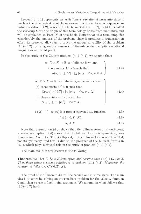
62 4 Evolutionary Variational Inequalities with Viscosity
Inequality (4.1) represents an evolutionary variational inequality since itinvolves the time derivative of the unknown function u. As a consequence, aninitial condition, (4.2), is needed. The term b(u(t), v − u(t)) in (4.1) is calledthe viscosity term; the origin of this terminology arises from mechanics andwill be explained in Part IV of this book. Notice that this term simplifiesconsiderably the analysis of the problem, since it produces a regularizationeffect; its presence allows us to prove the unique solvability of the problem(4.1)–(4.2) by using only arguments of time-dependent elliptic variationalinequalities and fixed point.
In the study of the Cauchy problem (4.1)–(4.2), we assume that:
a : X × X → R is a bilinear form and
there exists M > 0 such that
|a(u, v)| ≤ M‖u‖X‖v‖X ∀u, v ∈ X.
(4.3)
b : X × X → R is a bilinear symmetric form and
(a) there exists M ′ > 0 such that
|b(u, v)| ≤ M ′‖u‖X‖v‖X ∀u, v ∈ X.
(b) there exists m′ > 0 such that
b(v, v) ≥ m′‖v‖2X ∀ v ∈ X.
(4.4)
j : X → (−∞,∞] is a proper convex l.s.c. function. (4.5)
f ∈ C([0, T ];X). (4.6)
u0 ∈ X. (4.7)
Note that assumption (4.3) shows that the bilinear form a is continuous,whereas assumption (4.4) shows that the bilinear form b is symmetric, con-tinuous, and X-elliptic. The X-ellipticity of the bilinear form a is not needed,nor its symmetry, and this is due to the presence of the bilinear form b in(4.1), which plays a crucial role in the study of problem (4.1)–(4.2).
The main result of this section is the following.
Theorem 4.1. Let X be a Hilbert space and assume that (4.3)–(4.7) hold.Then there exists a unique solution u to problem (4.1)–(4.2). Moreover, thesolution satisfies u ∈ C1([0, T ];X).
The proof of the Theorem 4.1 will be carried out in three steps. The mainidea is to start by solving an intermediate problem for the velocity functionu and then to use a fixed point argument. We assume in what follows that(4.3)–(4.7) hold.

4.1 A Basic Existence and Uniqueness Result 63
In the first step, let η ∈ C([0, T ];X) be given and consider the problem offinding wη : [0, T ] → X such that
a(η(t), v − wη(t)) + b(wη(t), v − wη(t)) + j(v) − j(wη(t))
≥ (f(t), v − wη(t))X ∀ v ∈ X, t ∈ [0, T ]. (4.8)
The unique solvability of this problem is given by the following result.
Lemma 4.2. There exists a unique solution wη to the inequality (4.8). More-over, the solution satisfies wη ∈ C([0, T ];X).
Proof. We use (4.3) and Riesz’s representation theorem to define the functionfη : [0, T ] → X by
(fη(t), v)X = (f(t), v)X − a(η(t), v) ∀ v ∈ X, t ∈ [0, T ]. (4.9)
From assumption (4.3) on the form a, combined with the regularity f ∈C([0, T ];X) and η ∈ C([0, T ];X), it follows that fη ∈ C([0, T ];X). There-fore, assumptions (4.4) and (4.5) allow us to apply Theorem 3.12 to deducethat there exists a unique function wη ∈ C([0, T ];X) that solves the time-dependent variational inequality
b(wη(t), v − wη(t)) + j(v) − j(wη(t))
≥ (fη(t), v − wη(t))X ∀ v ∈ X, t ∈ [0, T ]. (4.10)
We combine (4.9) and (4.10) to see that the element wη ∈ C([0, T ];X) is theunique solution to the variational inequality (4.8). ⊓⊔
Next, we consider the operator Λ : C([0, T ];X) → C([0, T ];X) defined by
Λη(t) =
∫ t
0
wη(s)ds + u0 ∀ η ∈ C([0, T ];X), t ∈ [0, T ]. (4.11)
The second step is given by the following result.
Lemma 4.3. The operator Λ has a unique fixed point η∗ ∈ C([0, T ];X).
Proof. Let η1, η2 ∈ C([0, T ];X) and denote by wi the solution of (4.8) forη = ηi, i.e., wi = wηi
, i = 1, 2. From the definition (4.11), we deduce theinequality
‖Λη1(t) − Λη2(t)‖X ≤∫ t
0
‖w1(s) − w2(s)‖X ds ∀ t ∈ [0, T ]. (4.12)
On the other hand, using (4.8) for η = ηi, i = 1, 2, we obtain the inequality
b(w1(s) −w2(s), w1(s)−w2(s)) ≤ a(η1(s) − η2(s), w2(s) − w1(s)) ∀ s ∈ [0, T ]

64 4 Evolutionary Variational Inequalities with Viscosity
and, using the assumptions (4.3) and (4.4), we find
‖w1(s) − w2(s)‖X ≤ M
m′ ‖η1(s) − η2(s)‖X ∀ s ∈ [0, T ]. (4.13)
We combine inequalities (4.12) and (4.13) to obtain
‖Λη1(t) − Λη2(t)‖X ≤ c
∫ t
0
‖η1(s) − η2(s)‖X ds ∀ t ∈ [0, T ] (4.14)
with c =M
m′ . Lemma 4.3 is now a direct consequence of inequality (4.14) and
Lemma 1.42 (page 16). ⊓⊔
We now have all the ingredients to provide the proof of Theorem 4.1.
Proof. Existence. Let η∗ ∈ C([0, T ];X) be the fixed point of Λ and let u = η∗.Since η∗ = Λη∗, it follows from (4.11) that u(0) = u0 and u = wη∗ ; therefore,we conclude by (4.8) that u is a solution to problem (4.1)–(4.2). Moreover,since u = wη∗ and wη∗ ∈ C([0, T ];X), we deduce that u has the regularityu ∈ C1([0, T ];X).
Uniqueness. The uniqueness of the solution follows from the uniquenessof the fixed point of the operator Λ defined by (4.11), by using argumentssimilar to those used in the proof of the uniqueness part of Theorem 3.7. Italso can be obtained directly from (4.1)–(4.2), as follows: assume that u1,u2 ∈ C1([0, T ];X) are two solutions of (4.1)–(4.2) and let t ∈ [0, T ]. We have
a(u1(t), v − u1(t)) + b(u1(t), v − u1(t)) + j(v) − j(u1(t))
≥ (f(t), v − u1(t))X ∀ v ∈ X,
a(u2(t), v − u2(t)) + b(u2(t), v − u2(t)) + j(v) − j(u2(t))
≥ (f(t), v − u2(t))X ∀ v ∈ X.
We take v = u2(t) in the first inequality, v = u1(t) in the second one, andadd the results to obtain
b(u1(t) − u2(t), u1(t) − u2(t)) ≤ a(u1(t) − u2(t), u2(t) − u1(t)). (4.15)
We use now assumptions (4.3) and (4.4) to find
‖u1(t) − u2(t)‖X ≤ M
m′ ‖u1(t) − u2(t)‖X . (4.16)
Moreover, since ui(0) = u0 it follows that
ui(t) =
∫ t
0
ui(s) ds + u0 ∀ i = 1, 2, (4.17)

4.2 A Convergence Result 65
and, therefore,
‖u1(t) − u2(t)‖X ≤∫ t
0
‖u1(s) − u2(s)‖X ds. (4.18)
We combine now inequalities (4.16) and (4.18) and use Gronwall’s inequality(Lemma 1.44, page 17) to deduce the equality u1(s) = u2(s), for all s ∈ [0, T ];using then (4.17) we obtain that u1(t) = u2(t), which concludes the proof. ⊓⊔
Applying Theorem 4.1 to the case when j is the indicator function of anonempty, convex, and closed subset K ⊂ X leads to the following result.
Corollary 4.4. Let X be a Hilbert space, let K ⊂ X be a nonempty, convex,and closed subset, and assume that (4.3), (4.4), (4.6), (4.7) hold. Then thereexists a unique function u ∈ C1([0, T ];X) such that u(0) = u0 and
u(t) ∈ K, a(u(t), v − u(t)) + b(u(t), v − u(t))
≥ (f(t), v − u(t))X ∀ v ∈ K, t ∈ [0, T ].
We end this section with a regularity result.
Theorem 4.5. Under the conditions stated in Theorem 4.1, if there existsp ∈ [1,∞] such that f ∈ W 1,p(0, T ;X), then u ∈ W 2,p(0, T ;X).
Proof. For any t1, t2 ∈ [0, T ], we use (4.1) and the arguments used in theproof of (4.15) to obtain
b(u(t1) − u(t2), u(t1) − u(t2))
≤ a(u(t1) − u(t2), u(t2) − u(t1)) + (f(t1) − f(t2), u(t1)) − u(t2))X .
We employ now assumptions (4.3) and (4.4) to find
‖u(t1) − u(t2)‖X ≤ c (‖u(t1) − u(t2)‖X + ‖f(t1) − f(t2)‖X) (4.19)
where c = max Mm′
, 1m′
. This inequality combined with the regularity u ∈C1([0, T ];X), f ∈ W 1,p(0, T ;X) shows that u : [0, T ] → X is an absolutelycontinuous function and, moreover,
‖u(t)‖X ≤ c (‖u(t)‖X + ‖f(t)‖X) a.e. t ∈ (0, T ).
We conclude that u ∈ Lp(0, T ;X) and therefore u ∈ W 2,p(0, T ;X). ⊓⊔
4.2 A Convergence Result
In this section, we study the dependence of the solution of the variationalinequality (4.1)–(4.2) on the function j. To this end, we assume in what

66 4 Evolutionary Variational Inequalities with Viscosity
follows that (4.3)–(4.7) hold and we denote by u ∈ C1([0, T ];X) the solutionof (4.1)–(4.2) provided by Theorem 4.1.
For every ρ > 0, we also consider a perturbation jρ of j that satisfies(4.5) and we consider the problem of finding a function uρ : [0, T ] → X suchthat
a(uρ(t), v − uρ(t)) + b(uρ(t), v − uρ(t)) + jρ(v) − jρ(uρ(t))
≥ (f(t), v − uρ(t))X ∀ v ∈ X, t ∈ [0, T ], (4.20)
uρ(0) = u0. (4.21)
We deduce from Theorem 4.1 that problem (4.20)–(4.21) has a unique solu-tion uρ ∈ C1([0, T ];X), for each ρ > 0.
Our main result in this section is the following.
Theorem 4.6. Under the assumption (3.17), the solution uρ of problem(4.20)–(4.21) converges to the solution u of problem (4.1)–(4.2), i.e.,
‖uρ − u‖C1([0,T ];X) → 0 as ρ → 0. (4.22)
Proof. Let ρ > 0 and let t ∈ [0, T ]. We take v = uρ(t) in (4.1), v = u(t) in(4.20) and add the resulting inequalities to obtain
b(uρ(t) − u(t), uρ(t) − u(t)) ≤ a(uρ(t) − u(t), u(t) − uρ(t))
+j(uρ(t)) − j(u(t)) + jρ(u(t)) − jρ(uρ(t))
≤ a(uρ(t) − u(t), u(t) − uρ(t))
+ |j(uρ(t)) − jρ(uρ(t))| + |jρ(u(t)) − j(u(t))|.
We use assumptions (4.3), (4.4) and (3.17) to find that
m′‖uρ(t) − u(t)‖2X ≤ M‖uρ(t) − u(t)‖X‖uρ(t) − u(t)‖X + 2 F (ρ)
and, using the inequality
M‖uρ(t)−u(t)‖X‖uρ(t)−u(t)‖X ≤ M2
2m′ ‖uρ(t)−u(t)‖2X +
m′
2‖uρ(t)−u(t)‖2
X ,
we find that
‖uρ(t) − u(t)‖2X ≤ 4
m′ F (ρ) +M2
m′2 ‖uρ(t) − u(t)‖2X . (4.23)
It follows from (4.21) and (4.2) that
‖uρ(t) − u(t)‖X ≤∫ t
0
‖uρ(s) − u(s)‖X ds, (4.24)
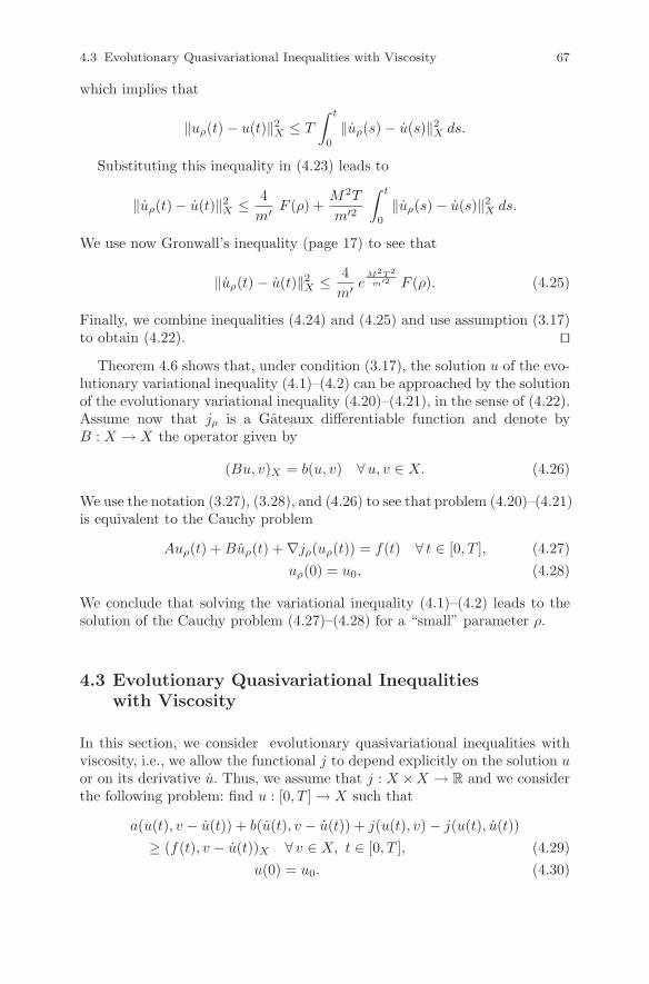
4.3 Evolutionary Quasivariational Inequalities with Viscosity 67
which implies that
‖uρ(t) − u(t)‖2X ≤ T
∫ t
0
‖uρ(s) − u(s)‖2X ds.
Substituting this inequality in (4.23) leads to
‖uρ(t) − u(t)‖2X ≤ 4
m′ F (ρ) +M2T
m′2
∫ t
0
‖uρ(s) − u(s)‖2X ds.
We use now Gronwall’s inequality (page 17) to see that
‖uρ(t) − u(t)‖2X ≤ 4
m′ eM2T2
m′2 F (ρ). (4.25)
Finally, we combine inequalities (4.24) and (4.25) and use assumption (3.17)to obtain (4.22). ⊓⊔
Theorem 4.6 shows that, under condition (3.17), the solution u of the evo-lutionary variational inequality (4.1)–(4.2) can be approached by the solutionof the evolutionary variational inequality (4.20)–(4.21), in the sense of (4.22).Assume now that jρ is a Gateaux differentiable function and denote byB : X → X the operator given by
(Bu, v)X = b(u, v) ∀u, v ∈ X. (4.26)
We use the notation (3.27), (3.28), and (4.26) to see that problem (4.20)–(4.21)is equivalent to the Cauchy problem
Auρ(t) + Buρ(t) + ∇jρ(uρ(t)) = f(t) ∀ t ∈ [0, T ], (4.27)
uρ(0) = u0. (4.28)
We conclude that solving the variational inequality (4.1)–(4.2) leads to thesolution of the Cauchy problem (4.27)–(4.28) for a “small” parameter ρ.
4.3 Evolutionary Quasivariational Inequalitieswith Viscosity
In this section, we consider evolutionary quasivariational inequalities withviscosity, i.e., we allow the functional j to depend explicitly on the solution uor on its derivative u. Thus, we assume that j : X × X → R and we considerthe following problem: find u : [0, T ] → X such that
a(u(t), v − u(t)) + b(u(t), v − u(t)) + j(u(t), v) − j(u(t), u(t))
≥ (f(t), v − u(t))X ∀ v ∈ X, t ∈ [0, T ], (4.29)
u(0) = u0. (4.30)

68 4 Evolutionary Variational Inequalities with Viscosity
We also consider the problem of finding u : [0, T ] → X such that
a(u(t), v − u(t)) + b(u(t), v − u(t)) + j(u(t), v) − j(u(t), u(t))
≥ (f(t), v − u(t))X ∀ v ∈ X, t ∈ [0, T ], (4.31)
u(0) = u0. (4.32)
In the study of these evolutionary quasivariational inequalities, we havethe following existence and uniqueness result.
Theorem 4.7. Let X be a Hilbert space and assume that (4.3), (4.4), (4.6),(4.7), and (3.30) hold. Then:
(1) There exists a unique solution u ∈ C1([0, T ];X) to problem (4.29)–(4.30).
(2) If m′ > α, there exists a unique solution u ∈ C1([0, T ];X) to problem(4.31)–(4.32).
Proof. (1) We use arguments similar to those used in the proof of Theo-rem 4.1, based on the unique solvability of time-dependent elliptic variationalinequalities and the Banach fixed point theorem. Since the modifications arestraightforward, we omit the details. The steps of the proof are the following.
(i) Let η ∈ C([0, T ];X) be given. We use Theorem 3.13 with Y = X tosee that there exists a unique element wη ∈ C([0, T ];X) such that
a(η(t), v − wη(t)) + b(wη(t), v − wη(t)) + j(η(t), v) − j(η(t), wη(t))
≥ (f(t), v − wη(t))X ∀ v ∈ X, t ∈ [0, T ]. (4.33)
(ii) Next, we consider the operator Λ : C([0, T ];X) → C([0, T ];X) definedby (4.11) and we prove that it has a unique fixed point η∗ ∈ C([0, T ];X).Indeed, let η1, η2 ∈ C([0, T ];X) and denote by wi the solutions of (4.33) forη = ηi, i.e., wi = wηi
, i = 1, 2. It follows that
b(w1(s) − w2(s), w1(s) − w2(s))
≤ a(η1(s) − η2(s), w2(s) − w1(s)) + j(η1(s), w2(s)) − j(η1(s), w1(s))
+ j(η2(s), w1(s)) − j(η2(s), w2(s)) ∀ s ∈ [0, T ]
and, using the assumptions (4.3), (4.4), and (3.30), we obtain
‖w1(s) − w2(s)‖X ≤ M + α
m′ ‖η1(s) − η2(s)‖X ∀s ∈ [0, T ]. (4.34)
We combine (4.12) and (4.34) to find (4.14) with c =M + α
m′ and then use
Lemma 1.42.
(iii) Let η∗ ∈ C([0, T ];X) be the fixed point of Λ and let u = η∗. Then itfollows that u is the unique solution of problem (4.29)–(4.30) and, moreover,it satisfies u ∈ C1([0, T ];X).

4.3 Evolutionary Quasivariational Inequalities with Viscosity 69
(2) This time we use arguments on time-dependent elliptic quasivariationalinequalities. The steps of the proof are the following.
(i) Let η ∈ C([0, T ];X) be given. We use Theorem 3.14 to see that, ifm′ > α, there exists a unique element wη ∈ C([0, T ];X) such that
a(η(t), v − wη(t)) + b(wη(t), v − wη(t)) + j(wη(t), v)
− j(wη(t), wη(t)) ≥ (f(t), v − wη(t))X ∀ v ∈ X, t ∈ [0, T ]. (4.35)
(ii) Next, we consider the operator Λ : C([0, T ];X) → C([0, T ];X) definedby (4.11) and we prove again that it has a unique fixed point. Indeed, if wi rep-resents the solution of (4.35) for η = ηi ∈ C([0, T ];X), i = 1, 2, it follows that
b(w1(s) − w2(s), w1(s) − w2(s))
≤ a(η1(s) − η2(s), w2(s) − w1(s)) + j(w1(s), w2(s)) − j(w1(s), w1(s))
+j(w2(s), w1(s)) − j(w2(s), w2(s)) ∀s ∈ [0, T ].
Now, by using assumptions (4.3), (4.4), (3.30) and the additional assumptionm′ > α, we find that
‖w1(s) − w2(s)‖X ≤ M
m′ − α‖η1(s) − η2(s)‖X ∀s ∈ [0, T ].
We combine this inequality with (4.12) to find (4.14) with c =M
m′ − αand
then use again Lemma 1.42.
(iii) Let η∗ ∈ C([0, T ];X) be the fixed point of Λ and let u = η∗. Then itfollows that u is the unique solution of problem (4.31)–(4.32) and, moreover,it satisfies u ∈ C1([0, T ];X). ⊓⊔
It follows from Theorem 4.7 that the unique solvability of the evolutionaryquasivariational inequalities (4.29)–(4.30) and (4.31)–(4.32), respectively, isproved under common assumptions that include (4.3), (4.4), (4.6), (4.7), and(3.30); also, note that the regularity u ∈ C1([0, T ];X) of the solution in bothof the two problems is the same. Therefore, we conclude that these varia-tional inequalities have similar features. However, we note that there exists adifference between these problems, and it arises from the fact that in solvingproblem (4.29)–(4.30), we do not need any additional assumptions, whereasin solving problem (4.31)–(4.32) we need to assume that m′ > α, which isa smallness assumption on the coefficient α. Examples of boundary valueproblems that lead to evolutionary quasivariational inequalities of the form(4.29)–(4.30) and (4.31)–(4.32) will be presented in Section 10.3 of the book.
We end this section with a regularity result, similar to that presented inTheorem 4.5.
Theorem 4.8. Under the conditions stated in Theorem 4.7, denote by u thesolution of problem (4.29)–(4.30) or (4.31)–(4.32) and assume, moreover, thatf ∈ W 1,p(0, T ;X) for some p ∈ [1,∞]. Then u ∈ W 2,p(0, T ;X).
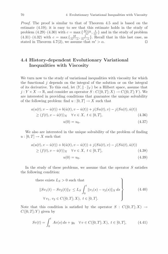
70 4 Evolutionary Variational Inequalities with Viscosity
Proof. The proof is similar to that of Theorem 4.5 and is based on theestimate (4.19); it is easy to see that this estimate holds in the study ofproblem (4.29)–(4.30) with c = max M+α
m′, 1
m′ and in the study of problem
(4.31)–(4.32) with c = max Mm′−α , 1
m′−α. Recall that in this last case, asstated in Theorem 4.7(2), we assume that m′ > α. ⊓⊔
4.4 History-dependent Evolutionary VariationalInequalities with Viscosity
We turn now to the study of variational inequalities with viscosity for whichthe functional j depends on the integral of the solution or on the integralof its derivative. To this end, let (Y, ‖ · ‖Y ) be a Hilbert space, assume thatj : Y ×X → R, and consider an operator S : C([0, T ];X) → C([0, T ];Y ). Weare interested in providing conditions that guarantee the unique solvabilityof the following problem: find u : [0, T ] → X such that
a(u(t), v − u(t)) + b(u(t), v − u(t)) + j(Su(t), v) − j(Su(t), u(t))
≥ (f(t), v − u(t))X ∀ v ∈ X, t ∈ [0, T ], (4.36)
u(0) = u0. (4.37)
We also are interested in the unique solvability of the problem of findingu : [0, T ] → X such that
a(u(t), v − u(t)) + b(u(t), v − u(t)) + j(Su(t), v) − j(Su(t), u(t))
≥ (f(t), v − u(t))X ∀ v ∈ X, t ∈ [0, T ], (4.38)
u(0) = u0. (4.39)
In the study of these problems, we assume that the operator S satisfiesthe following condition:
there exists LS > 0 such that
‖Sv1(t) − Sv2(t)‖Y ≤ LS
∫ t
0
‖v1(s) − v2(s)‖X ds
∀ v1, v2 ∈ C([0, T ];X), t ∈ [0, T ].
(4.40)
Note that this condition is satisfied by the operator S : C([0, T ];X) →C([0, T ];Y ) given by
Sv(t) =
∫ t
0
Av(s) ds + y0 ∀ v ∈ C([0, T ];X), t ∈ [0, T ], (4.41)

4.4 History-dependent Evolutionary Variational Inequalities with Viscosity 71
where A : X → Y is a Lipschitz continuous operator and y0 ∈ Y . It is alsosatisfied for the Volterra operator S : C([0, T ];X) → C([0, T ];Y ) given by
Sv(t) =
∫ t
0
A(t − s) v(s) ds + y0 ∀ v ∈ C([0, T ];X), t ∈ [0, T ], (4.42)
where now A ∈ C([0, T ];L(X, Y )) and, again, y0 ∈ Y . Indeed, in the caseof the operator (4.41), inequality (4.40) holds with LS being the Lipschitzconstant of the operator A, and in the case of the operator (4.42), it holds with
LS = ‖A‖C([0,T ];L(X,Y )) = maxt∈[0,T ]
‖A(t)‖L(X,Y ).
Clearly, for the operators (4.41) and (4.42), the current value Sv(t) at themoment t ∈ [0, T ] depends on the history of the values of v at the moments0 ≤ s ≤ t and, therefore, we refer to operators of the form (4.41) or (4.42)as history-dependent operators. We extend this definition to all the operatorsS : C([0, T ];X) → C([0, T ];Y ) satisfying condition (4.40) and, for this reason,we say that the variational inequalities (4.36)–(4.37) and (4.38)–(4.39) arehistory-dependent variational inequalities. Their new feature consists in thefact that, at each moment t ∈ [0, T ], the functional j depends on the historyof the solution up to the moment t, Su(t), or on the history of the derivativeof the solution up to the moment t, Su(t). This feature makes these problemsdifferent from the quasivariational inequalities studied in Section 4.3, sincethere j was assumed to depend on the current value of the solution, u(t), oron the current value of its derivative, u(t).
In the study of history-dependent evolutionary variational inequalitieswith viscosity, we have the following existence and uniqueness result.
Theorem 4.9. Let X and Y be two Hilbert spaces and assume that (4.3),(4.4), (4.6), (4.7), (3.54), and (4.40) hold. Then:
(1) There exists a unique solution u ∈ C1([0, T ];X) to problem (4.36)–(4.37).
(2) There exists a unique solution u ∈ C1([0, T ];X) to problem (4.38)–(4.39).
Proof. (1) We use arguments similar to those used in the proofs of Theo-rems 4.1 and 4.7 but with a different choice of the operator Λ. Below, c willrepresent various positive constants whose values may change from line toline. The steps of the proof are the following.
(i) Let η = (η1, η2) ∈ C([0, T ];X × Y ) be given. We use Theorem 3.13 tosee that there exists a unique element wη ∈ C([0, T ];X) such that
a(η1(t), v − wη(t)) + b(wη(t), v − wη(t)) + j(η2(t), v) − j(η2(t), wη(t))
≥ (f(t), v − wη(t))X ∀ v ∈ X, t ∈ [0, T ]. (4.43)

72 4 Evolutionary Variational Inequalities with Viscosity
(ii) We consider the operator Λ : C([0, T ];X × Y ) → C([0, T ];X × Y )defined by
Λη(t) =
(∫ t
0
wη(s) ds + u0, S
(∫ t
0
wη(s) ds + u0
))
∀ η ∈ C([0, T ];X × Y ), t ∈ [0, T ], (4.44)
and prove that Λ has a unique fixed point η∗. To this end, let η = (η1, η2)and ξ = (ξ1, ξ2) be two elements of C([0, T ];X × Y ) and denote by wη andwξ the corresponding solutions of inequality (4.43). After performing somealgebraic manipulations, we find
b(wη(s) − wξ(s), wη(s) − wξ(s))
≤ a(η1(s) − ξ1(s), wξ(s) − wη(s)) + j(η2(s), wξ(s)) − j(η2(s), wη(s))
+j(ξ2(s), wη(s)) − j(ξ2(s), wξ(s))
and, using assumptions (4.3), (4.4), and (3.54), we deduce that
‖wη(s) − wξ(s)‖X ≤ M
m′ ‖η1(s) − ξ1(s)‖X
+α
m′ ‖η2(s) − ξ2(s)‖Y ∀ s ∈ [0, T ]. (4.45)
We conclude by (4.45) that
‖wη(s) − wξ(s)‖X ≤ c ‖η(s) − ξ(s)‖X×Y ∀ s ∈ [0, T ] (4.46)
where ‖ · ‖X×Y denotes the norm on the space X × Y , given by
‖η‖X×Y =(‖η1‖2
X + ‖η2‖2Y
) 12 ∀ η = (η1, η2) ∈ X × Y.
Now, (4.44), (4.46), and (4.40) yield
‖Λη(t) − Λξ(t)‖X×Y
≤ c
∫ t
0
‖η(s) − ξ(s)‖X×Y + c
∫ t
0
(∫ s
0
‖η(r) − ξ(r)‖X×Y dr
)ds ∀ t ∈ [0, T ]
(4.47)
and, since
∫ t
0
(∫ s
0
‖η(r) − ξ(r)‖X×Y dr
)ds ≤ T
∫ t
0
‖η(s) − ξ(s)‖X×Y ds,
from (4.47) we obtain that
‖Λη(t) − Λξ(t)‖X×Y ≤ c
∫ t
0
‖η(s) − ξ(s)‖X×Y ds. (4.48)

4.4 History-dependent Evolutionary Variational Inequalities with Viscosity 73
Inequality (4.48) and Lemma 1.42 show that the operator Λ has a uniquefixed point.
(iii) Let η∗ = (η1∗, η2∗) ∈ C([0, T ];X ×Y ) be the fixed point of Λ and letu ∈ C1([0, T ];X) be the function defined by
u(t) =
∫ t
0
wη∗(s) ds + u0 ∀ t ∈ [0, T ]. (4.49)
It follows from (4.44) and (4.49) that
η1∗ = u, η2∗ = Su (4.50)
and, writing (4.43) for η = η∗ and using (4.50), we deduce that u satisfiesinequality (4.36). Also, (4.37) is a consequence of (4.49) and, since wη∗ ∈C([0, T ];X), we deduce that u ∈ C1([0, T ];X), which concludes the existencepart of Theorem 4.9(1).
(iv) The uniqueness part is a consequence of the uniqueness of the fixedpoint of the operator (4.44). It can also be obtained directly from (4.36),(4.37), as follows: assume that u1, u2 ∈ C1([0, T ];X) are two functionsthat satisfy (4.36)–(4.37) and let t ∈ [0, T ]. Then, after some algebra, weobtain
b(u1(t) − u2(t), u1(t) − u2(t))
≤ a(u1(t) − u2(t), u2(t) − u1(t)) + j(Su1(t), u2(t)) − j(Su1(t), u1(t))
+j(Su2(t), u1(t)) − j(Su2(t), u2(t)).
Next, using the assumptions (4.3), (4.4), (3.54), and (4.40), we find
‖u1(t) − u2(t)‖X ≤ c
(‖u1(t) − u2(t)‖X +
∫ t
0
‖u1(s) − u2(s)‖X ds
). (4.51)
Moreover, since ui(0) = u0, it follows that
ui(t) =
∫ t
0
ui(s) ds + u0 ∀ i = 1, 2 (4.52)
and, therefore,
‖u1(t) − u2(t)‖X ≤∫ t
0
‖u1(s) − u2(s)‖X ds. (4.53)
We combine now inequalities (4.51) and (4.53), and use Gronwall’s inequality(Lemma 1.44) to deduce that u1 = u2. Using (4.52), we obtain that u1(t) =u2(t), which concludes the uniqueness part of Theroem 4.9(1).
(2) The proof is similar to the proof of (1). The only difference consists inthe choice of the operator Λ : C([0, T ];X × Y ) → C([0, T ];X × Y ), which is

74 4 Evolutionary Variational Inequalities with Viscosity
now given by
Λη(t) =
(∫ t
0
wη(s) ds + u0, Swη(t)
)
∀ η ∈ C([0, T ];X × Y ), t ∈ [0, T ]. (4.54)
Using (4.40), it follows that inequality (4.48) still holds and, therefore, Λhas a unique fixed point η∗. Denote by u ∈ C1([0, T ];X) the function given by(4.49). It follows that u is a solution to problem (4.38)–(4.39) and, moreover,it is the unique solution of this Cauchy problem. ⊓⊔
Theorem 4.9 provides existence and uniqueness results in the study ofthe Cauchy problems (4.36)–(4.37) and (4.38)–(4.39), respectively, under thesame assumptions on the data; also, note that the regularity u ∈ C1(0, T ];X)of the solution is the same, in both the two problems above. Therefore, weconclude that the quasivariational inequalities (4.36)–(4.37) and (4.38)–(4.39)present a common feature. Moreover, we note that in comparison with The-orem 4.7, in Theorem 4.9 we do not need smallness assumptions in the studyof problem (4.38)–(4.39). This feature arises from the fact that in the proofof Theorem 4.9, we use assumption (4.40), which involves an integral termand allows us to derive inequality (4.48); and, as it follows from Lemma 1.42,inequalities of this form lead to a fixed point property without any smallnessassumption on the data. Examples of boundary value problems that lead toquasivariational inequalities of the form (4.36)–(4.37) or (4.38)–(4.39) will bepresented in Section 10.4 of the book.

Chapter 5
Evolutionary Variational Inequalities
In this chapter, we continue the study of evolutionary variational inequalitiesstarted in Chapter 4. The difference between the problems studied there andthose studied here lies in the fact that the variational inequalities presented inthis chapter do not involve a viscosity term. Their study is more complicated,since it cannot be done based on the unique solvability of time-dependentelliptic variational inequalities in velocities. We start with the study of evo-lutionary variational inequalities involving a differentiable functional j, forwhich we prove an existence and uniqueness result. The proof is based onthe study of a sequence of evolutionary variational inequalities with viscos-ity, compactness, and lower semicontinuity arguments. Then, we extend thisresult to a class of evolutionary variational inequalities for which the functionj can be approached, in a sense that will be described below, by a family ofdifferentiable functionals. We complete our results with a convergence resultthat shows that the solution of the evolutionary variational inequality withviscosity converges to the solution of the corresponding inviscid evolutionaryvariational inequality, as the viscosity converges to zero. Finally, we presentan existence result for evolutionary quasivariational inequalities, obtained byusing a time discretization method. The results presented in this chapter willbe applied in the study of quasistatic antiplane frictional contact problemswith elastic materials. As usual, everywhere in this chapter X is a real Hilbertspace with the inner product (·, ·)X and the norm ‖ · ‖X , and [0, T ] denotesthe time interval of interest, T > 0. Moreover, X is assumed to be separableeverywhere in Section 5.4 of this chapter.
5.1 A First Existence and Uniqueness Result
Let a be a bilinear form on X, j : X → (−∞,∞], f : [0, T ] → X and let u0
be the initial data. We are interested in providing sufficient conditions thatguarantee the existence of a unique solution of the following problem: find
75
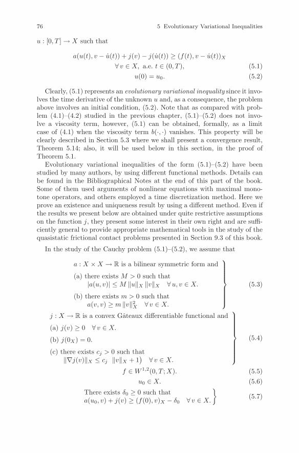
76 5 Evolutionary Variational Inequalities
u : [0, T ] → X such that
a(u(t), v − u(t)) + j(v) − j(u(t)) ≥ (f(t), v − u(t))X
∀ v ∈ X, a.e. t ∈ (0, T ), (5.1)
u(0) = u0. (5.2)
Clearly, (5.1) represents an evolutionary variational inequality since it invo-lves the time derivative of the unknown u and, as a consequence, the problemabove involves an initial condition, (5.2). Note that as compared with prob-lem (4.1)–(4.2) studied in the previous chapter, (5.1)–(5.2) does not invo-lve a viscosity term, however, (5.1) can be obtained, formally, as a limitcase of (4.1) when the viscosity term b(·, ·) vanishes. This property will beclearly described in Section 5.3 where we shall present a convergence result,Theorem 5.14; also, it will be used below in this section, in the proof ofTheorem 5.1.
Evolutionary variational inequalities of the form (5.1)–(5.2) have beenstudied by many authors, by using different functional methods. Details canbe found in the Bibliographical Notes at the end of this part of the book.Some of them used arguments of nonlinear equations with maximal mono-tone operators, and others employed a time discretization method. Here weprove an existence and uniqueness result by using a different method. Even ifthe results we present below are obtained under quite restrictive assumptionson the function j, they present some interest in their own right and are suffi-ciently general to provide appropriate mathematical tools in the study of thequasistatic frictional contact problems presented in Section 9.3 of this book.
In the study of the Cauchy problem (5.1)–(5.2), we assume that
a : X × X → R is a bilinear symmetric form and
(a) there exists M > 0 such that|a(u, v)| ≤ M ‖u‖X ‖v‖X ∀u, v ∈ X.
(b) there exists m > 0 such thata(v, v) ≥ m ‖v‖2
X ∀ v ∈ X.
(5.3)
j : X → R is a convex Gateaux differentiable functional and
(a) j(v) ≥ 0 ∀ v ∈ X.
(b) j(0X) = 0.
(c) there exists cj > 0 such that‖∇j(v)‖X ≤ cj
(‖v‖X + 1
)∀ v ∈ X.
(5.4)
f ∈ W 1,2(0, T ;X). (5.5)
u0 ∈ X. (5.6)
There exists δ0 ≥ 0 such thata(u0, v) + j(v) ≥ (f(0), v)X − δ0 ∀ v ∈ X.
(5.7)

5.1 A First Existence and Uniqueness Result 77
Note that assumption (5.4) combined with Corollary 2.33 provides sufficientconditions for the existence of the integrals below in this section, in whichthe functional j or its gadient ∇j appear.
Condition (5.7) represents a compatibility condition for the initial dataof problem (5.1)–(5.2). Such kind of conditions are usual in the study ofinviscid evolutionary variational inequalities. On occasions, assumption (5.7)is considered with δ0 = 0, as we shall do in Section 9.3 where we provide amechanical interpretation of this assumption.
Our main result in this section is the following.
Theorem 5.1. Let X be a Hilbert space and assume that (5.3)–(5.7) hold.Then there exists a unique solution u to problem (5.1)–(5.2) and it satisfiesu ∈ W 1,2(0, T ;X). Moreover, there exists a positive constant c, which doesnot depend on j, such that
‖u‖W 1,2(0,T ;X) ≤ c(√
δ0 + ‖u0‖X + ‖f‖W 1,2(0,T ;X)
). (5.8)
The proof of Theorem 5.1 will be carried out in several steps and is basedon the study of a sequence of evolutionary variational inequalities with viscos-ity, compactness, and lower semicontinuity arguments. We suppose in whatfollows that (5.3)–(5.7) hold, and, for every n ∈ N, we consider the problemof finding un : [0, T ] → X such that
a(un(t), v − un(t)) +1
n(un(t), v − un(t))X + j(v) − j(un(t))
≥ (f(t), v − un(t))X ∀ v ∈ X, t ∈ [0, T ]. (5.9)
un(0) = u0. (5.10)
Below in this section, c denotes a positive generic constant that may de-pend on a, T and on the function ϕ, which will be introduced later, but doesnot depend on n and j, nor on time, and whose value may change from lineto line.
In the first step, we provide the solvability of the problem (5.9)–(5.10),which represents an evolutionary variational inequality with viscosity.
Lemma 5.2. For every n ∈ N, there exists a unique solution un to the prob-lem (5.9)–(5.10). Moreover, the solution satisfies un ∈ W 2,2(0, T ;X).
Proof. Let n ∈ N and denote bn(u, v) = 1n (u, v)X for all u, v ∈ X. It is
clear that the form bn satisfies (4.4) and, moreover, (5.4) and Corollary 1.37imply that the function j is convex and lower semicontinuous. Lemma 5.2represents now a consequence of Theorems 4.1 and 4.5. ⊓⊔
In the next step, we provide some estimates of the solutions un on theinterval [0, T ].

78 5 Evolutionary Variational Inequalities
Lemma 5.3. There exists c > 0, which does not depend on j, such that theinequalities below hold, for all n ∈ N:
‖un‖C([0,T ];X) ≤ c (‖u0‖X + ‖f‖W 1,2(0,T ;X)), (5.11)
1√n
‖un‖L2(0,T ;X) ≤ c (‖u0‖X + ‖f‖W 1,2(0,T ;X)), (5.12)
∫ T
0
j(un(s)) ds ≤ c (‖u0‖2X + ‖f‖2
W 1,2(0,T ;X)). (5.13)
Proof. Let n ∈ N. We use (5.4) to see that the evolutionary variational ineq-uality (5.9) is equivalent to the variational equation
a(un(t), v) +1
n(un(t), v)X + (∇j(un(t)), v)X
= (f(t), v)X ∀ v ∈ X, t ∈ [0, T ] (5.14)
where ∇j denotes the gradient of the functional j, see Definition 1.35, page 14.Let s ∈ [0, T ]; we choose v = un(t) in (5.14) and integrate the resulting
equality on [0, s] to obtain∫ s
0
a(un(t), un(t)) dt +1
n
∫ s
0
(un(t), un(t))X dt +
∫ s
0
(∇j(un(t)), un(t))X dt
=
∫ s
0
(f(t), un(t))X dt. (5.15)
Next,∫ s
0
a(un(t), un(t)) dt =1
2
∫ s
0
d
dta(un(t), un(t)) dt
=1
2a(un(s), un(s)) − 1
2a(u0, u0), (5.16)
∫ s
0
(f(t), un(t))X dt
= (f(s), un(s))X − (f(0), un(0))X −∫ s
0
(f(t), un(t))X dt (5.17)
and∫ s
0
(∇j(un(t)), un(t))X dt ≥∫ s
0
j(un(t)) dt, (5.18)
where the inequality is obtained from the subgradient inequality
j(v) − j(un(t)) ≥ (∇j(un(t)), v − un(t)) ∀ v ∈ X
by choosing v = 0X , using the assumption that j(0X) = 0 and integratingthe result on [0, s].
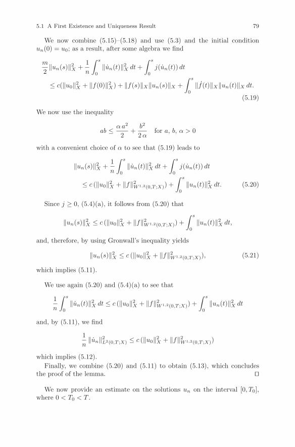
5.1 A First Existence and Uniqueness Result 79
We now combine (5.15)–(5.18) and use (5.3) and the initial conditionun(0) = u0; as a result, after some algebra we find
m
2‖un(s)‖2
X +1
n
∫ s
0
‖un(t)‖2X dt +
∫ s
0
j(un(t)) dt
≤ c(‖u0‖2X + ‖f(0)‖2
X) + ‖f(s)‖X‖un(s)‖X +
∫ s
0
‖f(t)‖X‖un(t)‖X dt.
(5.19)
We now use the inequality
ab ≤ α a2
2+
b2
2 αfor a, b, α > 0
with a convenient choice of α to see that (5.19) leads to
‖un(s)‖2X +
1
n
∫ s
0
‖un(t)‖2X dt +
∫ s
0
j(un(t)) dt
≤ c (‖u0‖2X + ‖f‖2
W 1,2(0,T ;X)) +
∫ s
0
‖un(t)‖2X dt. (5.20)
Since j ≥ 0, (5.4)(a), it follows from (5.20) that
‖un(s)‖2X ≤ c (‖u0‖2
X + ‖f‖2W 1,2(0,T ;X)) +
∫ s
0
‖un(t)‖2X dt,
and, therefore, by using Gronwall’s inequality yields
‖un(s)‖2X ≤ c (‖u0‖2
X + ‖f‖2W 1,2(0,T ;X)), (5.21)
which implies (5.11).
We use again (5.20) and (5.4)(a) to see that
1
n
∫ s
0
‖un(t)‖2X dt ≤ c (‖u0‖2
X + ‖f‖2W 1,2(0,T ;X)) +
∫ s
0
‖un(t)‖2X dt
and, by (5.11), we find
1
n‖un‖2
L2(0,T ;X) ≤ c (‖u0‖2X + ‖f‖2
W 1,2(0,T ;X))
which implies (5.12).
Finally, we combine (5.20) and (5.11) to obtain (5.13), which concludesthe proof of the lemma. ⊓⊔
We now provide an estimate on the solutions un on the interval [0, T0],where 0 < T0 < T .

80 5 Evolutionary Variational Inequalities
Lemma 5.4. For all 0 < T0 < T , there exists c(T0) > 0, which does notdepend on j, such that
‖un‖L2(0,T0;X) ≤ c(T0)(√
δ0 + ‖u0‖X + ‖f‖W 1,2(0,T ;X)), (5.22)
for all n ∈ N.
Proof. Let n ∈ N and consider a Lipschitz continuous function ϕ : [0, T ] → R
such that ϕ(t) > 0 for all t ∈ [0, T ) and ϕ(T ) = 0. We take v = ϕ(t)un(t) in(5.14) and integrate the result on [0, T ] to obtain
∫ T
0
ϕ(t) a(un(t), un(t)) dt +1
n
∫ T
0
ϕ(t) (un(t), un(t))X dt
+
∫ T
0
ϕ(t) (∇j(un(t)), un(t))X dt =
∫ T
0
ϕ(t) (f(t), un(t))X dt. (5.23)
We now perform integrations by parts and use the assumption ϕ(T ) = 0to see that
∫ T
0
ϕ(t) a(un(t), un(t)) dt
= −ϕ(0) a(un(0), un(0)) −∫ T
0
ϕ(t) a(un(t), un(t)) dt
−∫ T
0
ϕ(t) a(un(t), un(t)) dt, (5.24)
1
n
∫ T
0
ϕ(t) (un(t), un(t))X dt
= − 1
2n
[ϕ(0) (un(0), un(0))X +
∫ T
0
ϕ(t) (un(t), un(t))X dt
], (5.25)
∫ T
0
ϕ(t) (∇j(un(t)), un(t))X dt
=
∫ T
0
ϕ(t)d
dtj(un(t)) dt = −ϕ(0) j(un(0)) −
∫ T
0
ϕ(t) j(un(t)) dt, (5.26)
∫ T
0
ϕ(t) (f(t), un(t))X dt
= −ϕ(0) (f(0), un(0))X −∫ T
0
ϕ(t) (f(t), un(t))X dt
−∫ T
0
ϕ(t) (f(t), un(t))X dt. (5.27)

5.1 A First Existence and Uniqueness Result 81
We substitute equalities (5.24)–(5.27) in (5.23) and use the initial condition(5.10), assumption (5.7) with v = un(0), and inequality ϕ(0) > 0 to obtain
∫ T
0
ϕ(t) a(un(t), un(t)) dt
≤ δ0ϕ(0) − 1
2n
∫ T
0
ϕ(t) ‖un(t)‖2X dt −
∫ T
0
ϕ(t) j(un(t)) dt
−∫ T
0
ϕ(t) a(un(t), un(t)) dt +
∫ T
0
ϕ(t) (f(t), un(t))X dt
+
∫ T
0
ϕ(t) (f(t), un(t))X dt. (5.28)
On the other hand, we use (5.12) to see that
− 1
2n
∫ T
0
ϕ(t)‖un(t)‖2X dt ≤ c (‖u0‖2
X + ‖f‖2W 1,2(0,T ;X)) (5.29)
and we recall that here and below, c is a positive constant that depends on ϕbut is independent of j and n and whose value may change from place to place.
Also, inequality (5.13) implies that
−∫ T
0
ϕ(t) j(un(t)) dt ≤ c (‖u0‖2X + ‖f‖2
W 1,2(0,T ;X)). (5.30)
Assume now that |ϕ|√ϕ ∈ L∞(0, T ) and note that this additional assump-
tion is compatible with the previous assumption on ϕ since, for example, thefunction ϕ(t) = (T − t)2 satisfies all these requirements. With this additionalassumption on the function ϕ, we use (5.3) to see that
−∫ T
0
ϕ(t) a(un(t), un(t)) dt ≤ c
∫ T
0
√ϕ(t) ‖un(t)‖X‖un(t)‖X
|ϕ(t)|√ϕ(t)
dt
≤ c
∫ T
0
√ϕ(t) ‖un(t)‖X‖un(t)‖X dt
and, using the inequality
ab ≤ α a2
2+
b2
2 αfor a, b, α > 0,
we find that
−∫ T
0
ϕ(t)a(un(t), un(t))dt ≤ c
(α
∫ T
0
ϕ(t)‖un(t)‖2Xdt +
1
α
∫ T
0
‖un(t)‖2Xdt
),
(5.31)

82 5 Evolutionary Variational Inequalities
for all α > 0. Using similar arguments, it follows that
∫ T
0
ϕ(t) (f(t), un(t))X dt ≤ c
(α
∫ T
0
ϕ(t) ‖un(t)‖2X dt +
1
α
∫ T
0
‖f(t)‖2X dt
)
(5.32)
and
∫ T
0
ϕ(t) (f(t), un(t))X dt ≤ c
(α
∫ T
0
ϕ(t) ‖un(t)‖2X dt +
1
α
∫ T
0
‖f(t)‖2X dt
),
(5.33)
for all α > 0. We combine now (5.28)–(5.33), use (5.3), and choose a suffi-ciently small α to obtain that
∫ T
0
ϕ(t) ‖un(t)‖2X dt ≤ c
(δ0 + ‖u0‖2
X + ‖f‖2W 1,2(0,T ;X) +
∫ T
0
‖un(t)‖2X dt
).
We use now the previous inequality and (5.11) to see that
∫ T
0
ϕ(t) ‖un(t)‖2Xdt ≤ c (δ0 + ‖u0‖2
X + ‖f‖2W 1,2(0,T ;X)). (5.34)
Let T0 be such that 0 < T0 < T and choose ϕ such that the lower boundof ϕ on [0, T0], denoted l(T0), satisfies
l(T0) = inft∈[0,T0]
ϕ(t) > 0. (5.35)
For instance, take ϕ(t) = (T − t)2 to obtain l(T0) = (T − T0)2 > 0. Note
also that l(T0) depends on T0 but is independent on j and n. It follows from(5.34) and (5.35) that
l(T0)
∫ T0
0
‖un(t)‖2X dt ≤
∫ T0
0
ϕ(t) ‖un(t)‖2X dt
≤∫ T
0
ϕ(t) ‖un(t)‖2X dt
≤ c (δ0 + ‖u0‖2X + ‖f‖2
W 1,2(0,T ;X))
≤ c (√
δ0 + ‖u0‖X + ‖f‖W 1,2(0,T ;X))2.
This last inequality leads to (5.22) with c(T0) =√
cl(T0)
, which depends on
T0 but is independent on j and n. ⊓⊔
Inequality (5.11) shows that un is a bounded sequence in the spaceL∞(0, T ;X), and inequality (5.22) shows that, for all 0 < T0 < T, un

5.1 A First Existence and Uniqueness Result 83
is a bounded sequence in the space L2(0, T0;X). Therefore, there exists anelement u ∈ L∞(0, T ;X) such that for all 0 < T0 < T , the derivative ofu belongs to the space L2(0, T0;X) and there exists a subsequence of thesequence un, again denoted un, such that
un ∗ u in L∞(0, T ;X), (5.36)
un u in L2(0, T0;X). (5.37)
The convergences (5.36) and (5.37) imply that
un(t) u(t) in X, for all t ∈ [0, T0]. (5.38)
In the next lemma, we reinforce (5.38) by showing that, in fact, the seq-uence un(t) convergences strongly in X and uniformly with respect tot ∈ [0, T0]. Although this last result is not really necessary to the proof ofTheorem 5.1, we present it since it has interest in and of itself, and it isrelated to the convergence result presented in Section 5.3.
Lemma 5.5. Let 0 < T0 < T and consider a subsequence of the sequenceun, again denoted un, which satisfies (5.36) and (5.37). Then
‖un − u‖C([0,T0];X) → 0 as n → ∞. (5.39)
Proof. Let t ∈ [0, T ] and let p, n ∈ N such that p > n. It follows from (5.9)that
a(un(t), up(t) − un(t)) +1
n(un(t), up(t) − un(t))X + j(up(t)) − j(un(t))
≥ (f(t), up(t) − un(t))X
and
a(up(t), un(t) − up(t)) +1
p(up(t), un(t) − up(t))X + j(un(t)) − j(up(t))
≥ (f(t), un(t) − up(t))X .
We add the two inequalities to obtain
a(un(t) − up(t), un(t) − up(t))
≤(
1
pup(t) − 1
nun(t), un(t) − up(t)
)
X
≤(
1
p‖up(t)‖X +
1
n‖un(t)‖X
)(‖un(t)‖X + ‖up(t)‖X)
≤ 2
n(‖un(t)‖2
X + ‖up(t)‖2X).
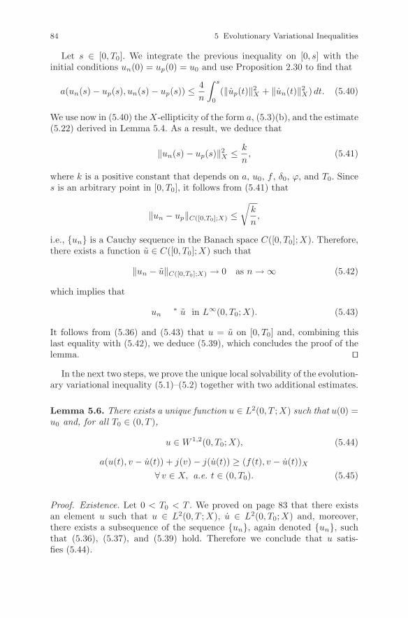
84 5 Evolutionary Variational Inequalities
Let s ∈ [0, T0]. We integrate the previous inequality on [0, s] with theinitial conditions un(0) = up(0) = u0 and use Proposition 2.30 to find that
a(un(s) − up(s), un(s) − up(s)) ≤ 4
n
∫ s
0
(‖up(t)‖2X + ‖un(t)‖2
X) dt. (5.40)
We use now in (5.40) the X-ellipticity of the form a, (5.3)(b), and the estimate(5.22) derived in Lemma 5.4. As a result, we deduce that
‖un(s) − up(s)‖2X ≤ k
n, (5.41)
where k is a positive constant that depends on a, u0, f , δ0, ϕ, and T0. Sinces is an arbitrary point in [0, T0], it follows from (5.41) that
‖un − up‖C([0,T0];X) ≤√
k
n,
i.e., un is a Cauchy sequence in the Banach space C([0, T0];X). Therefore,there exists a function u ∈ C([0, T0];X) such that
‖un − u‖C([0,T0];X) → 0 as n → ∞ (5.42)
which implies that
un ∗ u in L∞(0, T0;X). (5.43)
It follows from (5.36) and (5.43) that u = u on [0, T0] and, combining thislast equality with (5.42), we deduce (5.39), which concludes the proof of thelemma. ⊓⊔
In the next two steps, we prove the unique local solvability of the evolution-ary variational inequality (5.1)–(5.2) together with two additional estimates.
Lemma 5.6. There exists a unique function u ∈ L2(0, T ;X) such that u(0) =u0 and, for all T0 ∈ (0, T ),
u ∈ W 1,2(0, T0;X), (5.44)
a(u(t), v − u(t)) + j(v) − j(u(t)) ≥ (f(t), v − u(t))X
∀ v ∈ X, a.e. t ∈ (0, T0). (5.45)
Proof. Existence. Let 0 < T0 < T . We proved on page 83 that there existsan element u such that u ∈ L2(0, T ;X), u ∈ L2(0, T0;X) and, moreover,there exists a subsequence of the sequence un, again denoted un, suchthat (5.36), (5.37), and (5.39) hold. Therefore we conclude that u satis-fies (5.44).

5.1 A First Existence and Uniqueness Result 85
Consider now an element v ∈ L2(0, T0;X); we use v(t) as the test functionin (5.9) and integrate the result on [0, T0] to obtain, for all n ∈ N,
∫ T0
0
a(un(t), v(t) − un(t)) dt +1
n
∫ T0
0
(un(t), v(t) − un(t))X dt +
∫ T0
0
j(v(t))dt
≥∫ T0
0
j(un(t))dt +
∫ T0
0
(f(t), v(t) − un(t))X dt. (5.46)
It follows from (5.37), (5.39), and (5.3) that
limn→∞
∫ T0
0
a(un(t), v(t) − un(t)) dt =
∫ T0
0
a(u(t), v(t) − u(t)) dt (5.47)
and using (5.22) yields
limn→∞
1
n
∫ T0
0
(un(t), v(t) − un(t))X dt = 0. (5.48)
Also, assumption (5.4) on the function j, Corollary 2.33, and (5.37) imply that
lim infn→∞
∫ T0
0
j(un(t)) dt ≥∫ T0
0
j(u(t)) dt (5.49)
and, again, (5.37) leads to
limn→∞
∫ T0
0
(f(t), v(t) − un(t))Xdt =
∫ T0
0
(f(t), v(t) − u(t))X dt. (5.50)
We pass to the lower limit in (5.46) and use (5.47)–(5.50) to obtain
∫ T0
0
a(u(t), v(t) − u(t)) dt +
∫ T0
0
j(v(t))dt −∫ T0
0
j(u(t)) dt
≥∫ T0
0
(f(t), v(t) − u(t))X dt.
Since the previous inequality is valid for all v ∈ L2(0, T0;X), a classical ap-plication of the Lebesgue point for L1 functions (Theorem 2.20 on page 34,see also [57, p. 165]) shows that u satisfies (5.45).
Finally, (5.10) and (5.39) imply that u(0) = u0, which concludes the exis-tence part of the theorem.
Uniqueness. Consider two functions u1, u2 ∈ L2(0, T ;X) such that u1(0) =u2(0) = u0, which satisfy (5.44), (5.45), for all 0 < T0 < T . Let s ∈ (0, T )and let T0 be such that s < T0 < T . We have
a(u1(t), v − u1(t)) + j(v) − j(u1(t)) ≥ (f(t), v − u1(t))X ,
a(u2(t), v − u2(t)) + j(v) − j(u2(t)) ≥ (f(t), v − u2(t))X ,

86 5 Evolutionary Variational Inequalities
for all v ∈ X, a.e. t ∈ (0, T0). We take v = u2(t) in the first inequality,v = u1(t) in the second one, add the resulting inequalities, and use Proposi-tion 2.30 to obtain
1
2
d
dta(u1(t) − u2(t), u1(t) − u2(t)) ≤ 0 a.e. t ∈ (0, T0).
We integrate the previous inequality on [0, s] with the initial conditionsu1(0) = u2(0) = u0 and use assumption (5.3)(b) on a to see that
m ‖u1(s) − u2(s)‖2X ≤ 0.
This inequality shows that u1(s) = u2(s) for all s ∈ (0, T ), i.e., u1 = u2. ⊓⊔
Lemma 5.7. Let u be the function defined in Lemma 5.6. Then:(1) There exists c > 0, which does not depend on j, such that
‖u‖L2(0,T ;X) ≤ c (‖u0‖X + ‖f‖W 1,2(0,T ;X)). (5.51)
(2) For all 0 < T0 < T , there exists c(T0) > 0, which does not depend onj, such that
‖u‖L2(0,T0;X) ≤ c(T0)(√
δ0 + ‖u0‖X + ‖f‖W 1,2(0,T ;X)). (5.52)
Proof. (1) We use (5.36) to see that un u weakly in L2(0, T ;X) and, sincethe arguments presented on page 13 show that v → ‖v‖L2(0,T ;X) is a l.s.c.functional on the space L2(0, T ;X), we find that
‖u‖L2(0,T ;X) ≤ lim infn→∞
‖un‖L2(0,T ;X). (5.53)
Also, since ‖un‖L2(0,T ;X) ≤√
T ‖un‖C([0,T ];X) for all n ∈ N, it follows from(5.11) that
‖un‖L2(0,T ;X) ≤ c (‖u0‖X + ‖f‖W 1,2(0,T ;X)) ∀n ∈ N (5.54)
where, again, c is a positive constant that does not depend on n and j.Estimate (5.51) is now a consequence of (5.53) and (5.54).
(2) Let 0 < T0 < T. We use (5.37), (5.22), and the lower semicotinuity ofthe norm on the space L2(0, T0;X) to see that
‖u‖L2(0,T0;X) ≤ lim infn→∞
‖un‖L2(0,T0;X)
≤ c(T0)(√
δ0 + ‖u0‖X + ‖f‖W 1,2(0,T ;X)),
which concludes the proof. ⊓⊔
We have now all the ingredients needed to prove Theorem 5.1.

5.1 A First Existence and Uniqueness Result 87
Proof. Existence. Let T1 > T ; we extend the function f : [0, T ] → X to afunction f1 : [0, T1] → X given by
f1(t) =
f(t) if 0 ≤ t ≤ T,
f(T ) if T < t ≤ T1.(5.55)
We note that (5.5) implies the regularity f1 ∈ W 1,2(0, T1;X), and (5.7)still holds if we replace f(0) by f1(0). Therefore, we are allowed to apply Lem-mas 5.6 and 5.7 on the time interval (0, T1), replacing f with f1; as a result,we obtain that there exists a unique function u1 ∈ L2(0, T1;X) such that
u1(0) = u0 (5.56)
and, for all T0 ∈ (0, T1),
u1 ∈ W 1,2(0, T0;X), (5.57)
a(u1(t), v − u1(t)) + j(v) − j(u1(t))
≥ (f1(t), v − u1(t))X ∀ v ∈ X, a.e. t ∈ (0, T0), (5.58)
‖u1‖L2(0,T0;X) ≤ c(T0)(√
δ0 + ‖u0‖X + ‖f1‖W 1,2(0,T1;X)), (5.59)
where c(T0) > 0 does not depend on j.Let u∗ be the restriction of u1 to [0, T ], i.e.,
u∗(t) = u1(t) ∀ t ∈ [0, T ]. (5.60)
We take T0 = T < T1 and use (5.56)–(5.58) to see that u∗ is a solution ofproblem (5.1)–(5.2) and satisfies u∗ ∈ W 1,2(0, T ;X).
Uniqueness. The uniqueness of the solution follows directly from (5.1)–(5.2), by using the same arguments as those used in the proof of the unique-ness part of Lemma 5.6.
Estimate. We use (5.59) with T0 = T < T1 and (5.60) to obtain that
‖u∗‖L2(0,T ;X) ≤ c(T )(√
δ0 + ‖u0‖X + ‖f1‖W 1,2(0,T1;X)
)
and, since (5.55) implies that
‖f1‖W 1,2(0,T1;X) ≤ (1 + c√
T1 − T ) ‖f‖W 1,2(0,T ;X),
we find that
‖u∗‖L2(0,T ;X) ≤ c(T ) (√
δ0 + ‖u0‖X + (1 + c√
T1 − T ) ‖f‖W 1,2(0,T ;X)).(5.61)
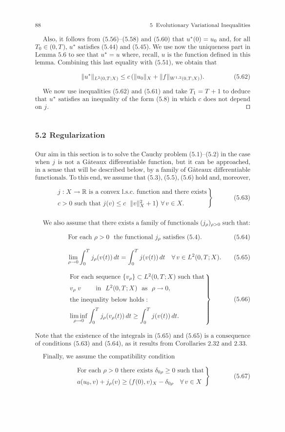
88 5 Evolutionary Variational Inequalities
Also, it follows from (5.56)–(5.58) and (5.60) that u∗(0) = u0 and, for allT0 ∈ (0, T ), u∗ satisfies (5.44) and (5.45). We use now the uniqueness part inLemma 5.6 to see that u∗ = u where, recall, u is the function defined in thislemma. Combining this last equality with (5.51), we obtain that
‖u∗‖L2(0,T ;X) ≤ c (‖u0‖X + ‖f‖W 1,2(0,T ;X)). (5.62)
We now use inequalities (5.62) and (5.61) and take T1 = T + 1 to deducethat u∗ satisfies an inequality of the form (5.8) in which c does not dependon j. ⊓⊔
5.2 Regularization
Our aim in this section is to solve the Cauchy problem (5.1)–(5.2) in the casewhen j is not a Gateaux differentiable function, but it can be approached,in a sense that will be described below, by a family of Gateaux differentiablefunctionals. To this end, we assume that (5.3), (5.5), (5.6) hold and, moreover,
j : X → R is a convex l.s.c. function and there exists
c > 0 such that j(v) ≤ c(‖v‖2
X + 1)
∀ v ∈ X.
(5.63)
We also assume that there exists a family of functionals (jρ)ρ>0 such that:
For each ρ > 0 the functional jρ satisfies (5.4). (5.64)
limρ→0
∫ T
0
jρ(v(t)) dt =
∫ T
0
j(v(t)) dt ∀ v ∈ L2(0, T ;X). (5.65)
For each sequence vρ ⊂ L2(0, T ;X) such that
vρ v in L2(0, T ;X) as ρ → 0,
the inequality below holds :
lim infρ→0
∫ T
0
jρ(vρ(t)) dt ≥∫ T
0
j(v(t)) dt.
(5.66)
Note that the existence of the integrals in (5.65) and (5.65) is a consequenceof conditions (5.63) and (5.64), as it results from Corollaries 2.32 and 2.33.
Finally, we assume the compatibility condition
For each ρ > 0 there exists δ0ρ ≥ 0 such that
a(u0, v) + jρ(v) ≥ (f(0), v)X − δ0ρ ∀ v ∈ X
(5.67)
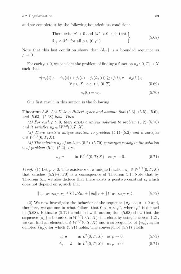
5.2 Regularization 89
and we complete it by the following boundedness condition:
There exist ρ∗ > 0 and M∗ > 0 such that
δ0ρ < M∗ for all ρ ∈ (0, ρ∗).
(5.68)
Note that this last condition shows that δ0ρ is a bounded sequence asρ → 0.
For each ρ > 0, we consider the problem of finding a function uρ : [0, T ]→ Xsuch that
a(uρ(t), v − uρ(t)) + jρ(v) − jρ(uρ(t)) ≥ (f(t), v − uρ(t))X
∀ v ∈ X, a.e. t ∈ (0, T ), (5.69)
uρ(0) = u0. (5.70)
Our first result in this section is the following.
Theorem 5.8. Let X be a Hilbert space and assume that (5.3), (5.5), (5.6),and (5.63)–(5.68) hold. Then:
(1) For each ρ > 0, there exists a unique solution to problem (5.2)–(5.70)and it satisfies uρ ∈ W 1,2(0, T ;X).
(2) There exists a unique solution to problem (5.1)–(5.2) and it satisfiesu ∈ W 1,2(0, T ;X).
(3) The solution uρ of problem (5.2)–(5.70) converges weakly to the solutionu of problem (5.1)–(5.2), i.e.,
uρ u in W 1,2(0, T ;X) as ρ → 0. (5.71)
Proof. (1) Let ρ > 0. The existence of a unique function uρ ∈ W 1,2(0, T ;X)that satisfies (5.2)–(5.70) is a consequence of Theorem 5.1. Note that byTheorem 5.1, we also deduce that there exists a positive constant c, whichdoes not depend on ρ, such that
‖uρ‖W 1,2(0,T ;X) ≤ c (√
δ0ρ + ‖u0‖X + ‖f‖W 1,2(0,T ;X)). (5.72)
(2) We now investigate the behavior of the sequence uρ as ρ → 0 and,therefore, we assume in what follows that 0 < ρ < ρ∗, where ρ∗ is definedin (5.68). Estimate (5.72) combined with assumption (5.68) show that thesequence uρ is bounded in W 1,2(0, T ;X); therefore, by using Theorem 1.21,we can find an element u ∈ W 1,2(0, T ;X) and a subsequence of uρ, againdenoted uρ, for which (5.71) holds. The convergence (5.71) yields
uρ u in L2(0, T ;X) as ρ → 0, (5.73)
uρ u in L2(0, T ;X) as ρ → 0. (5.74)

90 5 Evolutionary Variational Inequalities
Let v ∈ L2(0, T ;X); we integrate (5.2) on [0, T ] with the initial condition(5.70) to obtain
∫ T
0
a(uρ(t), v(t)) dt +
∫ T
0
jρ(v(t)) dt
≥ 1
2a(uρ(T ), uρ(T )) − 1
2a(u0, u0) +
∫ T
0
jρ(uρ(t)) dt
+
∫ T
0
(f(t), v(t) − uρ(t))X dt. (5.75)
Then, we use (5.73), (5.74), the properties of the bilinear form a, (5.3), andassumptions (5.65), (5.65) to see that
limρ→0
∫ T
0
a(uρ(t), v(t)) dt =
∫ T
0
a(u(t), v(t)) dt, (5.76)
lim infρ→0
1
2a(uρ(T ), uρ(T )) ≥ 1
2a(u(T ), u(T )), (5.77)
limρ→0
∫ T
0
jρ(v(t)) dt =
∫ T
0
j(v(t)) dt, (5.78)
lim infρ→0
∫ T
0
jρ(uρ(t)) dt ≥∫ T
0
j(u(t)) dt, (5.79)
limρ→0
∫ T
0
(f(t), v(t) − uρ(t))X dt =
∫ T
0
(f(t), v(t) − u(t))X dt. (5.80)
Next, we pass to the lower limit in (5.75) as ρ → 0 and use (5.76)–(5.80) toobtain
∫ T
0
a(u(t), v(t)) dt +
∫ T
0
j(v(t)) dt
≥ 1
2a(u(T ), u(T )) − 1
2a(u0, u0) +
∫ T
0
j(u(t)) dt
+
∫ T
0
(f(t), v(t) − u(t))X dt. (5.81)
It follows from the convergences (5.73) and (5.74) that uρ(t)u(t) in X forall t ∈ [0, T ] and, using (5.70), we deduce that u satisfies (5.2). This last equal-ity and the properties of a combined with Proposition 2.30 on page 37 yield
∫ T
0
a(u(t), u(t)) dt =1
2a(u(T ), u(T )) − 1
2a(u0, u0). (5.82)
We now use (5.81) and (5.82) to see that u satisfies the inequality
∫ T
0
a(u(t), v(t) − u(t)) dt +
∫ T
0
(j(v(t)) − j(u(t))) dt ≥∫ T
0
(f(t), v(t)−u(t))Xdt.

5.2 Regularization 91
Then, performing a localization argument by applying Theorem 2.20 onpage 34, we obtain that u satisfies (5.1).
We conclude that the element u ∈ W 1,2(0, T ;X) defined above is a solu-tion to problem (5.1)–(5.2), which proves the existence of a solution to thisCauchy problem. The uniqueness of the solution follows by using the argu-ments already used on page 85, in the proof of Lemma 5.6.
(3) Consider a subsequence of the sequence uρ, again denoted uρ, andan element w ∈ W 1,2(0, T ;X) such that
uρ w in W 1,2(0, T ;X) as ρ → 0.
It follows from the arguments above that w is a solution to problem (5.1)–(5.2) and therefore, since this last problem has a unique solution denoted u,we find that w = u. We conclude that the weak limit in W 1,2(0, T ;X) isindependent of the subsequence extracted and, therefore, the whole sequenceuρ converges weakly in W 1,2(0, T ;X) to u, i.e., (5.71) holds. ⊓⊔
Given a family of functionals jρ that satisfies (5.64), it is sometimesdifficult to check conditions (5.65)–(5.65), as well as conditions (5.67)–(5.68).Moreover, note that conditions (5.67)–(5.68) do not represent intrinsic condi-tions on the initial data of the evolutionary variational inequality (5.1)–(5.2),as they are related to the family of functionals jρ that regularize j. For thesereasons, in what follows we replace conditions (5.65)–(5.65) with condition(3.17), already used in Chapters 3 and 4. The interest in this last conditionis that it is time independent and therefore it can be easily checked. Also, wereplace assumptions (5.67)–(5.68) on the initial data with assumption (5.7).As we shall see in the two lemmas below, condition (3.17) is stronger than con-ditions (5.65)–(5.65) and, combined with assumption (5.7), allows us to obt-ain a version of Theorem 5.8 in which assumptions (5.65)–(5.68) are avoided.
Lemma 5.9. Assume (5.63) and (5.64). Then condition (3.17) implies con-ditions (5.65) and (5.65).
Proof. Let ρ > 0, v ∈ L2(0, T ;X) and assume that (3.17) holds. We use thiscondition to see that
∣∣∣∣∫ T
0
jρ(v(t)) dt −∫ T
0
j(v(t)) dt
∣∣∣∣ ≤∫ T
0
|jρ(v(t)) − j(v(t))| dt
≤∫ T
0
F (ρ) dt ≤ F (ρ) T
and therefore, since F (ρ) → 0 as ρ → 0, we deduce that (5.65) holds.Consider now a sequence vρ ⊂ L2(0, T ;X) and let v ∈ L2(0, T ;X) be
such that
vρ v in L2(0, T ;X). (5.83)

92 5 Evolutionary Variational Inequalities
We have∫ T
0
jρ(vρ(t)) dt =
∫ T
0
(jρ(vρ(t)) − j(vρ(t))
)dt +
∫ T
0
j(vρ(t)) dt ∀ ρ > 0
and, since (3.17) implies that
limρ→0
∫ T
0
(jρ(vρ(t)) − j(vρ(t))
)dt = 0,
we deduce that
lim infρ→0
∫ T
0
jρ(vρ(t)) dt = lim infρ→0
∫ T
0
j(vρ(t)) dt. (5.84)
The convergence (5.83), assumption (5.63), and the lower semicontinuity res-ult in Corollary 2.32 yield
lim infρ→0
∫ T
0
j(vρ(t)) dt ≥∫ T
0
j(v(t)) dt. (5.85)
We use now (5.84) and (5.85) to see that (5.65) holds. ⊓⊔
Lemma 5.10. Assume (5.3), (5.5)–(5.7). Then condition (3.17) implies con-ditions (5.67) and (5.68).
Proof. Let ρ > 0 and assume that (3.17) holds. We use (5.7) and (3.17)(a)to see that
a(u0, v) + jρ(v) − (f(0), v)X ≥ jρ(v) − j(v) − δ0 ≥ −δ0 − F (ρ) ∀ v ∈ X
and therefore condition (5.67) holds with δ0ρ = δ0 + F (ρ).Next, it follows from (3.17)(b) that there exists ρ∗ > 0 such that F (ρ) < 1
for all ρ ∈ (0, ρ∗). We conclude that δ0ρ < δ0 + 1 for all ρ ∈ (0, ρ∗) andtherefore condition (5.68) holds with M∗ = δ0 + 1. ⊓⊔
We now use Lemmas 5.9 and 5.10 to obtain the following version of The-orem 5.8.
Theorem 5.11. Let X be a Hilbert space and assume that (5.3), (5.5)–(5.7),(5.63), (5.64), and (3.17) hold. Then:
(1) For each ρ > 0 there exists a unique solution to problem (5.2)–(5.70)and it satisfies uρ ∈ W 1,2(0, T ;X).
(2) There exists a unique solution to problem (5.1)–(5.2) and it satisfiesu ∈ W 1,2(0, T ;X).
(3) The solution uρ of problem (5.2)–(5.70) converges uniformly to thesolution u of problem (5.1)–(5.2), i.e.,
uρ → u in C([0, T ], X) as ρ → 0. (5.86)

5.2 Regularization 93
Proof. The first two parts of the theorem are direct consequences of Lem-mas 5.9 and 5.10 combined with Theorem 5.8(1), (2). Therefore, we have toprove only the convergence result (5.86). To this end, consider ρ > 0 andchoose v = uρ(t) in (5.1) and v = u(t) in (5.2); we add the resulting inequal-ities to find
a(uρ(t) − u(t), uρ(t) − u(t))
≤ j(uρ(t)) − jρ(uρ(t)) + jρ(u(t)) − j(u(t)) a.e. t ∈ (0, T ).
We use now assumption (3.17)(a) to see that
j(uρ(t)) − jρ(uρ(t)) + jρ(u(t)) − j(u(t)) ≤ 2F (ρ) a.e. t ∈ (0, T )
and, therefore, combining the last two inequalities yields
a(uρ(t) − u(t), uρ(t) − u(t)) ≤ 2F (ρ) a.e. t ∈ (0, T ). (5.87)
Let s ∈ [0, T ]. We integrate (5.87) on [0, s] with the initial conditions uρ(0) =u0, u(0) = u0, then we use Proposition 2.30 and (5.3)(b); as a result, we find
‖uρ(s) − u(s)‖2X ≤ 4T
mF (ρ)
which, combined with (3.17)(b), implies (5.86). ⊓⊔
The interest in Theorems 5.8 and 5.11 is twofold; first, these theorems pro-vide existence and uniqueness results in the study of the evolutionary vari-ational inequality (5.1)–(5.2) in the case when j is not necessary a Gateauxdifferentiable function; secondly, they show that the solution u of problem(5.1)–(5.2) can be obtained as limit of the solutions uρ of problem (5.2)–(5.70), in the sense of (5.71) and (5.86), respectively.
The assumptions made in Theorems 5.8 and 5.11 require the function jto be approached by a sequence of functionals, jρ, which are more regular,since they are Gateaux differentiable. For this reason, the method used inthe proof of Theorems 5.8 and 5.11 is called the regularization method. Itsmain feature consists in proving the existence of the solution of an “irreg-ular” variational inequality as limit of the solutions of “regular” variationalinequalities.
We end this section with the remark that the existence of a unique solutionto the Cauchy problem (5.1)–(5.2) can be obtained under weaker assumptionsthat those in Theorems 5.1, 5.8, and 5.11. Indeed, the following existence anduniqueness result represents a direct version of a result proved in [16, p. 117].
Theorem 5.12. Let X be a Hilbert space and assume that (5.3), (5.5)–(5.7),(4.5) hold. Then there exists a unique solution of the evolutionary variationalinequality (5.1)–(5.2) and it satisfies u ∈ W 1,2(0, T ;X).
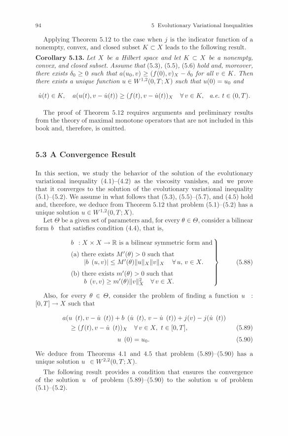
94 5 Evolutionary Variational Inequalities
Applying Theorem 5.12 to the case when j is the indicator function of anonempty, convex, and closed subset K ⊂ X leads to the following result.
Corollary 5.13. Let X be a Hilbert space and let K ⊂ X be a nonempty,convex, and closed subset. Assume that (5.3), (5.5), (5.6) hold and, moreover,there exists δ0 ≥ 0 such that a(u0, v) ≥ (f(0), v)X − δ0 for all v ∈ K. Thenthere exists a unique function u ∈ W 1,2(0, T ;X) such that u(0) = u0 and
u(t) ∈ K, a(u(t), v − u(t)) ≥ (f(t), v − u(t))X ∀ v ∈ K, a.e. t ∈ (0, T ).
The proof of Theorem 5.12 requires arguments and preliminary resultsfrom the theory of maximal monotone operators that are not included in thisbook and, therefore, is omitted.
5.3 A Convergence Result
In this section, we study the behavior of the solution of the evolutionaryvariational inequality (4.1)–(4.2) as the viscosity vanishes, and we provethat it converges to the solution of the evolutionary variational inequality(5.1)–(5.2). We assume in what follows that (5.3), (5.5)–(5.7), and (4.5) holdand, therefore, we deduce from Theorem 5.12 that problem (5.1)–(5.2) has aunique solution u ∈ W 1,2(0, T ;X).
Let Θ be a given set of parameters and, for every θ ∈ Θ, consider a bilinearform bθ that satisfies condition (4.4), that is,
bθ : X × X → R is a bilinear symmetric form and
(a) there exists M ′(θ) > 0 such that|bθ(u, v)| ≤ M ′(θ)‖u‖X‖v‖X ∀u, v ∈ X.
(b) there exists m′(θ) > 0 such thatbθ(v, v) ≥ m′(θ)‖v‖2
X ∀ v ∈ X.
(5.88)
Also, for every θ ∈ Θ, consider the problem of finding a function uθ :[0, T ] → X such that
a(uθ(t), v − uθ(t)) + bθ(uθ(t), v − uθ(t)) + j(v) − j(uθ(t))
≥ (f(t), v − uθ(t))X ∀ v ∈ X, t ∈ [0, T ], (5.89)
uθ(0) = u0. (5.90)
We deduce from Theorems 4.1 and 4.5 that problem (5.89)–(5.90) has aunique solution uθ ∈ W 2,2(0, T ;X).
The following result provides a condition that ensures the convergenceof the solution uθ of problem (5.89)–(5.90) to the solution u of problem(5.1)–(5.2).

5.3 A Convergence Result 95
Theorem 5.14. Under the previous assumptions,
M ′(θ)2
m′(θ)→ 0 =⇒ ‖uθ − u‖C([0,T ];X) → 0. (5.91)
The convergence (5.91) is understood in the sense described on page 48,
i.e., for every sequence θn ⊂ Θ such that M ′(θn)2
m′(θn) → 0 as n → ∞, one has
‖uθn− u‖C([0,T ];X) as n → ∞.
Proof. The equalities and inequalities below hold for almost every t ∈ (0, T ).We choose v = u(t) in (5.89), v = uθ(t) in (5.1), and add the resultinginequalities to obtain
a(uθ(t) − u(t), u(t) − uθ(t)) + bθ(uθ(t), u(t) − uθ(t)) ≥ 0.
This implies that
a(uθ(t) − u(t), uθ(t) − u(t)) + bθ(uθ(t) − u(t), uθ(t) − u(t))
≤ bθ(u(t), u(t) − uθ(t))
and, using assumption (5.88), yields
a(uθ(t) − u(t), uθ(t) − u(t)) + m′(θ)‖uθ(t) − u(t)‖2X
≤ M ′(θ) ‖u(t)‖X‖uθ(t) − u(t)‖X . (5.92)
We now combine (5.92) with the elementary inequality
‖u(t)‖X ‖uθ(t) − u(t)‖X ≤ M ′(θ)
4m′(θ)‖u(t)‖2
X +m′(θ)
M ′(θ)‖uθ(t) − u(t)‖2
X
and, as a result, we obtain
a(uθ(t) − u(t), uθ(t) − u(t)) ≤ M ′(θ)2
4m′(θ)‖u(t)‖2
X .
Let s ∈ [0, T ]. We integrate the previous inequality on [0, s] with the initialconditions uθ(0) = u(0) = u0 and use assumption (5.3) to obtain
m
2‖uθ(s) − u(s)‖2
X ≤ M ′(θ)2
4m′(θ)
∫ s
0
‖u(t)‖2X dt.
This last inequality shows that
‖uθ(s) − u(s)‖X ≤√
M ′(θ)2
2mm′(θ)‖u‖L2(0,T ;X). (5.93)

96 5 Evolutionary Variational Inequalities
Assume now that
M ′(θ)2
m′(θ)→ 0. (5.94)
Then, it follows from estimate (5.93) that ‖uθ − u‖C([0,T ];X) → 0, whichcompletes the proof. ⊓⊔
We conclude from Theorem 5.14 that we can approach the solution of theinviscid evolutionary variational inequality (5.1)–(5.2) with the solution ofthe evolutionary variational inequality with viscosity (5.89)–(5.90) if the ratioM ′(θ)2
m′(θ) is small enough. Note that we already used a similar result in the proof
of Theorem 5.1. Indeed, there we have considered the regularized problems(5.9)–(5.10), which are of the form (5.89)–(5.90) with θ = 1
n and bθ(u, v) =1n (u, v)X . It is clear that in this case (5.94) holds as n → ∞ and, therefore,by Theorem 5.14 we recover the convergence result presented in Lemma 5.5.
Finally, a brief comparison between the results presented in Section 4.1 inthe study of evolutionary variational inequality with viscosity (Theorems 4.1and 4.5) and the results presented in Sections 5.1 and 5.2 in the study of invi-scid evolutionary variational inequalities (Theorems 5.1, 5.8, 5.11 and 5.12)leads to the following remarks:
(a) Under the same regularity (say f ∈ W 1,2(0, T ;X) and u0 ∈ X) onthe data, the regularity of the solution of problem (4.1)–(4.2) is higher thanthe regularity of the solution of problem (5.1)–(5.2) (W 2,2(0, T ;X) insteadof W 1,2(0, T ;X), respectively);
(b) To solve problem (5.1)–(5.2), one needs a compatibility assumptionon the initial data ((5.7) or (5.67), (5.68)); in contrast, to solve problem(4.1)–(4.2), such an assumption is not needed.
The two remarks above lead to the conclusion that adding viscosity has asmoothing effect on the solution of evolutionary variational inequalities. Thisfeature combined with the convergence result (5.91) justifies the use of numer-ical methods based on regularization with viscosity in the study of (5.1)–(5.2).
5.4 Evolutionary Quasivariational Inequalities
In this section, we study an evolutionary version of the quasivariationalinequality (3.29). To this end, we assume in what follows that X is a separableHilbert space and let a : X × X → R, j : X × X → R, f : [0, T ] → X begiven. We consider the problem of finding a function u : [0, T ] → X such that
a(u(t), v − u(t)) + j(u(t), v) − j(u(t), u(t))
≥ (f(t), v − u(t))X ∀ v ∈ X, a.e. t ∈ (0, T ), (5.95)
u(0) = u0. (5.96)
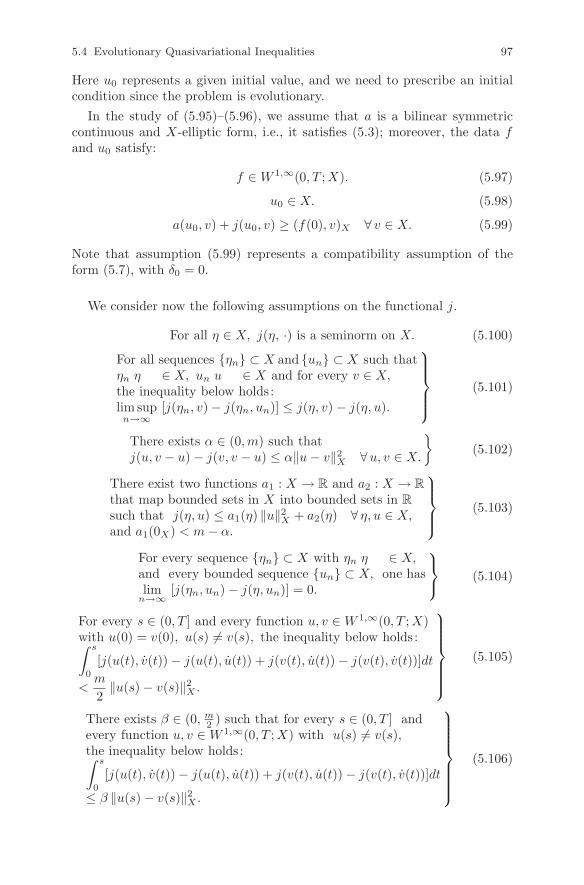
5.4 Evolutionary Quasivariational Inequalities 97
Here u0 represents a given initial value, and we need to prescribe an initialcondition since the problem is evolutionary.
In the study of (5.95)–(5.96), we assume that a is a bilinear symmetriccontinuous and X-elliptic form, i.e., it satisfies (5.3); moreover, the data fand u0 satisfy:
f ∈ W 1,∞(0, T ;X). (5.97)
u0 ∈ X. (5.98)
a(u0, v) + j(u0, v) ≥ (f(0), v)X ∀ v ∈ X. (5.99)
Note that assumption (5.99) represents a compatibility assumption of theform (5.7), with δ0 = 0.
We consider now the following assumptions on the functional j.
For all η ∈ X, j(η, ·) is a seminorm on X. (5.100)
For all sequences ηn ⊂ X and un ⊂ X such thatηn η ∈ X, un u ∈ X and for every v ∈ X,the inequality below holds :lim sup
n→∞[j(ηn, v) − j(ηn, un)] ≤ j(η, v) − j(η, u).
(5.101)
There exists α ∈ (0, m) such thatj(u, v − u) − j(v, v − u) ≤ α‖u − v‖2
X ∀u, v ∈ X.
(5.102)
There exist two functions a1 : X → R and a2 : X → R
that map bounded sets in X into bounded sets in R
such that j(η, u) ≤ a1(η) ‖u‖2X + a2(η) ∀ η, u ∈ X,
and a1(0X) < m − α.
(5.103)
For every sequence ηn ⊂ X with ηn η ∈ X,and every bounded sequence un ⊂ X, one haslim
n→∞[j(ηn, un) − j(η, un)] = 0.
(5.104)
For every s ∈ (0, T ] and every function u, v ∈ W 1,∞(0, T ;X)with u(0) = v(0), u(s) = v(s), the inequality below holds :∫ s
0
[j(u(t), v(t)) − j(u(t), u(t)) + j(v(t), u(t)) − j(v(t), v(t))]dt
<m
2‖u(s) − v(s)‖2
X .
(5.105)
There exists β ∈ (0, m2 ) such that for every s ∈ (0, T ] and
every function u, v ∈ W 1,∞(0, T ;X) with u(s) = v(s),the inequality below holds :∫ s
0
[j(u(t), v(t)) − j(u(t), u(t)) + j(v(t), u(t)) − j(v(t), v(t))]dt
≤ β ‖u(s) − v(s)‖2X .
(5.106)

98 5 Evolutionary Variational Inequalities
Note that assumptions (5.100) and (5.101) have already been used inSection 3.4 in the study of elliptic quasivariational inequalities, see (3.36)and (3.37), respectively.
Our main result in the study of problem (5.95)–(5.96) is the following.
Theorem 5.15. Let X be a separable Hilbert space and assume that (5.3)and (5.97)–(5.99) hold. Then:
(1) Under the assumptions (5.100)–(5.104), there exists at least one solu-tion u ∈ W 1,∞(0, T ;X) to problem (5.95)–(5.96).
(2) Under the assumptions (5.100)–(5.105), there exists a unique solutionu ∈ W 1,∞(0, T ;X) to problem (5.95)–(5.96).
(3) Under the assumptions (5.100)–(5.104) and (5.106), there exists aunique solution u = u(f, u0) ∈ W 1,∞(0, T ;X) to problem (5.95)–(5.96), andthe mapping (f, u0) → u is Lipschitz continuous from W 1,∞(0, T ;X) × X toC([0, T ];X).
The proof of Theorem 5.15 will be carried out in several steps by usinga time discretization method, compactness and lower semicontinuity argu-ments. We suppose in what follows that (5.3), (5.97)–(5.104) hold. Letn ∈ N. We consider the following implicit scheme: find ui+1
n ∈ X suchthat
a
(ui+1
n , v − n
T(ui+1
n − uin)
)+ j(ui+1
n , v) − j
(ui+1
n ,n
T(ui+1
n − uin)
)
≥(
f
(T (i + 1)
n
), v − n
T(ui+1
n − uin)
)
X
∀ v ∈ X, (5.107)
where u0n = u0, i = 0, 1, . . . , n − 1.
In the first step, we prove the solvability of the elliptic quasivariationalinequality (5.107) and we provide estimates on the solution to this problem.
Lemma 5.16. There exists at least one solution ui+1n to the quasivaria-
tional inequality (5.107), for i = 0, 1, . . . , n − 1. Moreover, the solutionsatisfies
‖ui+1n ‖2
X ≤ 1
m − α − a1(0X)
(∥∥∥∥f(
T (i + 1)
n
)∥∥∥∥X
‖ui+1n ‖X + a2(0X)
),
(5.108)
‖ui+1n − ui
n‖X ≤ 1
m − α
∥∥∥∥f(
T (i + 1)
n
)− f
(Ti
n
)∥∥∥∥X
, (5.109)
for all i = 0, 1, . . . , n − 1.

5.4 Evolutionary Quasivariational Inequalities 99
Proof. Let i ∈ 0, 1, . . . , n − 1. We set w = Tn v + ui
n and use the propertiesof a and j to see that (5.107) is equivalent to the inequality
a(ui+1n , w − ui+1
n ) + j(ui+1n , w − ui
n) − j(ui+1n , ui+1
n − uin)
≥(
f
(T (i + 1)
n
), w − ui+1
n
)
X
∀w ∈ X. (5.110)
Using Theorem 3.10(1), we obtain the existence of a solution ui+1n to (5.110)
and, therefore, the equivalence of problems (5.107) and (5.110) yields the firstpart of the lemma.
Choosing now w = 0X in (5.110) and using (5.100), we find
a(ui+1n , ui+1
n ) ≤(
f
(T (i + 1)
n
), ui+1
n
)
X
+ j(ui+1n ,−ui
n) − j(ui+1n , ui+1
n − uin)
≤∥∥∥∥f(
T (i + 1)
n
)∥∥∥∥X
‖ui+1n ‖X + j(ui+1
n ,−ui+1n ),
and using (5.3)(b) yields
m ‖ui+1n ‖2
X ≤∥∥∥∥f(
T (i + 1)
n
)∥∥∥∥X
‖ui+1n ‖X + j(ui+1
n ,−ui+1n ). (5.111)
Choosing u = ui+1n and v = 0X in (5.102) and using (5.103) with η = 0X , we
obtain
j(ui+1n ,−ui+1
n ) ≤ α ‖ui+1n ‖2
X + j(0X ,−ui+1n )
≤ (α + a1(0X)) ‖ui+1n ‖2
X + a2(0X). (5.112)
Estimate (5.108) results from (5.111) and (5.112), since a1(0X) < m − α.
Using (5.100), it follows that
j(u, 0X) = 0 ∀u ∈ X (5.113)
and therefore, by setting w = uin in (5.110) and using (5.113), we obtain
a(ui+1n , ui+1
n − uin) ≤
(f
(T (i + 1)
n
), ui+1
n − uin
)
X
− j(ui+1n , ui+1
n − uin) ∀ i = 0, 1, . . . , n − 1. (5.114)
Using again (5.110) with i − 1 in place of i and w = ui+1n , we find
a(uin, ui+1
n − uin) + j(ui
n, ui+1n − ui−1
n ) − j(uin, ui
n − ui−1n )
≥(
f
(Ti
n
), ui+1
n − uin
)
X
∀ i = 1, . . . , n − 1

100 5 Evolutionary Variational Inequalities
and, using (5.100), we obtain
−a(uin, ui+1
n − uin) ≤ −
(f
(Ti
n
), ui+1
n − uin
)
X
+ j(uin, ui+1
n − uin) ∀ i = 1, . . . , n − 1.
Note that, since u0n = u0, assumption (5.99) yields
−a(u0n, u1
n − u0n) ≤ −(f(0), u1
n − u0n)X + j(u0
n, u1n − u0
n).
We conclude by the last two inequalities that
−a(uin, ui+1
n − uin) ≤ −
(f
(Ti
n
), ui+1
n − uin
)
X
+ j(uin, ui+1
n − uin) ∀ i = 0, 1, . . . , n − 1. (5.115)
It follows now from (5.3)(b), (5.114), (5.115), and (5.102) that
m ‖ui+1n − ui
n‖2X
≤ a(ui+1n − ui
n, ui+1n − ui
n)
≤(
f
(T (i + 1)
n
)− f
(Ti
n
), ui+1
n − uin
)
X
− j(ui+1n , ui+1
n − uin) + j(ui
n, ui+1n − ui
n)
≤∥∥∥∥f(
T (i + 1)
n
)− f
(Ti
n
)∥∥∥∥X
‖ui+1n − ui
n‖X + α ‖ui+1n − ui
n‖2X
∀ i = 0, 1, . . . , n − 1,
which implies (5.109). ⊓⊔
We now consider the functions un : [0, T ] → X and un : [0, T ] → X definedas follows:
un(0) = u0, un(t) = uin +
nt − Ti
T(ui+1
n − uin)
∀ t ∈(
Ti
n,T (i + 1)
n
], (5.116)
un(0) = u0, un(t) = ui+1n ∀ t ∈
(Ti
n,T (i + 1)
n
], (5.117)
where u0n = u0, ui+1
n solves (5.107) and i = 0, 1, . . . , n − 1.
In the next step, we provide convergence results involving the sequencesun and un.
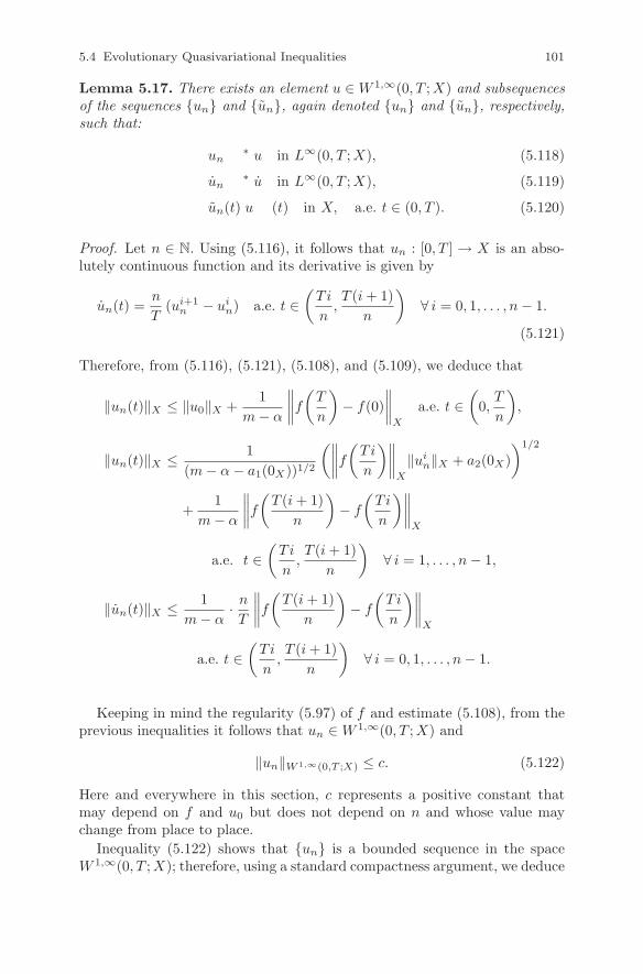
5.4 Evolutionary Quasivariational Inequalities 101
Lemma 5.17. There exists an element u ∈ W 1,∞(0, T ;X) and subsequencesof the sequences un and un, again denoted un and un, respectively,such that:
un ∗ u in L∞(0, T ;X), (5.118)
un ∗ u in L∞(0, T ;X), (5.119)
un(t) u(t) in X, a.e. t ∈ (0, T ). (5.120)
Proof. Let n ∈ N. Using (5.116), it follows that un : [0, T ] → X is an abso-lutely continuous function and its derivative is given by
un(t) =n
T(ui+1
n − uin) a.e. t ∈
(Ti
n,T (i + 1)
n
)∀ i = 0, 1, . . . , n − 1.
(5.121)
Therefore, from (5.116), (5.121), (5.108), and (5.109), we deduce that
‖un(t)‖X ≤ ‖u0‖X +1
m − α
∥∥∥∥f(
T
n
)− f(0)
∥∥∥∥X
a.e. t ∈(
0,T
n
),
‖un(t)‖X ≤ 1
(m − α − a1(0X))1/2
(∥∥∥∥f(
Ti
n
)∥∥∥∥X
‖uin‖X + a2(0X)
)1/2
+1
m − α
∥∥∥∥f(
T (i + 1)
n
)− f
(Ti
n
)∥∥∥∥X
a.e. t ∈(
Ti
n,T (i + 1)
n
)∀ i = 1, . . . , n − 1,
‖un(t)‖X ≤ 1
m − α· n
T
∥∥∥∥f(
T (i + 1)
n
)− f
(Ti
n
)∥∥∥∥X
a.e. t ∈(
Ti
n,T (i + 1)
n
)∀ i = 0, 1, . . . , n − 1.
Keeping in mind the regularity (5.97) of f and estimate (5.108), from theprevious inequalities it follows that un ∈ W 1,∞(0, T ;X) and
‖un‖W 1,∞(0,T ;X) ≤ c. (5.122)
Here and everywhere in this section, c represents a positive constant thatmay depend on f and u0 but does not depend on n and whose value maychange from place to place.
Inequality (5.122) shows that un is a bounded sequence in the spaceW 1,∞(0, T ;X); therefore, using a standard compactness argument, we deduce

102 5 Evolutionary Variational Inequalities
that there exists an element u ∈ W 1,∞(0, T ;X) and a subsequence of un,again denoted un, such that (5.118) and (5.119) hold.
We turn now to the proof of (5.120). To this end, we remark that theconvergences (5.118) and (5.119) imply that
un(t) u(t) in X, for all t ∈ [0, T ]. (5.123)
Moreover, using again (5.116), (5.117), and (5.109), we find
‖un(t) − un(t)‖X =
(1 − nt − Ti
T
)‖ui+1
n − uin‖X
≤ 1
m − α
∥∥∥∥f(
T (i + 1)
n
)− f
(Ti
n
)∥∥∥∥X
∀ t ∈(
Ti
n,T (i + 1)
n
], i = 0, 1, . . . , n − 1
and, keeping in mind the regularity (5.97) of f , we deduce that
‖un − un‖L∞(0,T ;X) ≤ T
n(m − α)‖f‖L∞(0,T ;X).
This inequality proves that
un − un → 0 in L∞(0, T ;X) (5.124)
and, therefore,
un(t) − un(t) → 0 in X, a.e. t ∈ (0, T ). (5.125)
The convergence (5.120) is now a consequence of (5.123) and (5.125). ⊓⊔
In the next two steps, we prove additional convergence and semicontinuityresults. To this end, for every n ∈ N consider the function fn : [0, T ] → Xdefined as follows:
fn(0) = f(0), fn(t) = f
(T (i + 1)
n
)(5.126)
∀ t ∈(
Ti
n,T (i + 1)
n
], i = 0, 1, . . . , n − 1.
Everywhere in the sequel, u will denote an element of W 1,∞(0, T ;X) thatsatisfies the properties in Lemma 5.17 and un, un, fn will representappropriate subsequences of the sequences un, un and fn, respectively,which satisfy (5.118)–(5.120).

5.4 Evolutionary Quasivariational Inequalities 103
Lemma 5.18. The following properties hold:
limn→∞
∫ T
0
a(un(t), g(t)) dt =
∫ T
0
a(u(t), g(t)) dt ∀ g ∈ L2(0, T ;X), (5.127)
lim infn→∞
∫ T
0
a(un(t), un(t)) dt ≥∫ T
0
a(u(t), u(t)) dt, (5.128)
limn→∞
∫ T
0
(fn(t), g(t) − un(t))X dt
=
∫ T
0
(f(t), g(t) − u(t))X dt ∀ g ∈ L2(0, T ;X). (5.129)
Proof. It follows from convergences (5.118) and (5.124) that un u inL2(0, T ;X) and therefore, by using (5.3), we deduce (5.127). Using again(5.3)(a), (5.124), and (5.122), we find
limn→∞
∫ T
0
a(un(t) − un(t), un(t)) dt = 0 (5.130)
and, from (5.123), un(0) = u0, and semicontinuity arguments already usedin this chapter, we obtain
lim infn→∞
∫ T
0
a(un(t), un(t)) dt ≥∫ T
0
a(u(t), u(t)) dt. (5.131)
The inequality (5.128) is now a consequence of (5.130) and (5.131).
Finally, from (5.97) and (5.126), we obtain that the sequence fn con-verges uniformly to f on [0, T ], i.e.,
maxt∈[0,T ]
‖fn(t) − f(t)‖X → 0 as n → ∞. (5.132)
The convergence (5.129) is now a consequence of (5.119) and (5.132). ⊓⊔
Lemma 5.19. The following properties hold:
lim supn→∞
∫ T
0
j(un(t), g(t)) dt ≤∫ T
0
j(u(t), g(t)) dt ∀ g ∈ L2(0, T ;X),
(5.133)
lim supn→∞
∫ T
0
[j(u(t), un(t)) − j(un(t), un(t))] dt ≤ 0, (5.134)
lim infn→∞
∫ T
0
j(u(t), un(t)) dt ≥∫ T
0
j(u(t), u(t)) dt. (5.135)
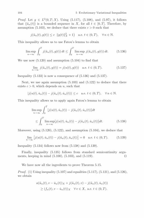
104 5 Evolutionary Variational Inequalities
Proof. Let g ∈ L2(0, T ;X). Using (5.117), (5.108), and (5.97), it followsthat un(t) is a bounded sequence in X, for all t ∈ [0, T ]. Therefore, byassumption (5.103), we deduce that there exists c > 0 such that
j(un(t), g(t)) ≤ c(‖g(t)‖2
X + 1)
a.e. t ∈ (0, T ), ∀n ∈ N.
This inequality allows us to use Fatou’s lemma to obtain
lim supn→∞
∫ T
0
j(un(t), g(t)) dt ≤∫ T
0
lim supn→∞
j(un(t), g(t)) dt. (5.136)
We use now (5.120) and assumption (5.104) to find that
limn→∞
j(un(t), g(t)) = j(u(t), g(t)) a.e. t ∈ (0, T ). (5.137)
Inequality (5.133) is now a consequence of (5.136) and (5.137).
Next, we use again assumption (5.103) and (5.122) to deduce that thereexists c > 0, which depends on u, such that
|j(u(t), un(t)) − j(un(t), un(t))| ≤ c a.e. t ∈ (0, T ), ∀n ∈ N.
This inequality allows us to apply again Fatou’s lemma to obtain
lim supn→∞
∫ T
0
[j(u(t), un(t)) − j(un(t), un(t))]dt
≤∫ T
0
lim supn→∞
[j(u(t), un(t)) − j(un(t), un(t))]dt. (5.138)
Moreover, using (5.120), (5.122), and assumption (5.104), we deduce that
limn→∞
[j(u(t), un(t)) − j(un(t), un(t))
]= 0 a.e. t ∈ (0, T ). (5.139)
Inequality (5.134) follows now from (5.138) and (5.139).
Finally, inequality (5.135) follows from standard semicontinuity argu-ments, keeping in mind (5.100), (5.103), and (5.119). ⊓⊔
We have now all the ingredients to prove Theorem 5.15.
Proof. (1) Using inequality (5.107) and equalities (5.117), (5.121), and (5.126),we obtain
a(un(t), v − un(t))X + j(un(t), v) − j(un(t), un(t))
≥ (fn(t), v − un(t))X ∀ v ∈ X, a.e. t ∈ (0, T ).

5.4 Evolutionary Quasivariational Inequalities 105
This inequality and assumption (5.103) yield
∫ T
0
a(un(t), g(t) − un(t)) dt +
∫ T
0
j(un(t), g(t)) dt −∫ T
0
j(un(t), un(t)) dt
≥∫ T
0
(fn(t), g(t) − un(t)X) dt ∀ g ∈ L2(0, T ;X).
Using now (5.127)–(5.129), (5.133)–(5.135), by passing to the lower limit inthe previous inequality we find
∫ T
0
a(u(t), g(t) − u(t)) dt +
∫ T
0
j(u(t), g(t)) dt −∫ T
0
j(u(t), u(t)) dt
≥∫ T
0
(f(t), g(t) − u(t))X dt ∀ g ∈ L2(0, T ;X). (5.140)
We now use in (5.140) a classical application of Lebesgue point for L1 func-tions, Theorem 2.20, and obtain that u ∈ W 1,∞(0, T ;X) satisfies inequality(5.95); moreover, from (5.116) and (5.123) we deduce (5.96), which concludesthe proof of this part of the theorem.
(2) Consider two solutions u1, u2 ∈ W 1,∞(0, T ;X) to the Cauchy problem(5.95)–(5.96). The inequalities below hold for all v ∈ X and a.e. t ∈ (0, T ):
a(u1(t), v − u1(t)) + j(u1(t), v) − j(u1(t), u1(t)) ≥ (f(t), v − u1(t))X ,
a(u2(t), v − u2(t)) + j(u2(t), v) − j(u2(t), u2(t)) ≥ (f(t), v − u2(t))X .
We take v = u2(t) in the first inequality, v = u1(t) in the second inequality,then we add the resulting inequalities and use (5.3) to obtain
1
2
d
dta(u1(t) − u2(t), u1(t) − u2(t))
≤ j(u1(t), u2(t)) − j(u1(t), u1(t)) + j(u2(t), u1(t))
−j(u2(t), u2(t)) a.e. t ∈ (0, T ). (5.141)
Moreover, from (5.96) we have
u1(0) = u2(0) = u0. (5.142)
Arguing by contradiction, let us suppose that u1 = u2. Then there existss ∈ (0, T ] such that
u1(s) = u2(s). (5.143)

106 5 Evolutionary Variational Inequalities
Integrating (5.141) over [0, s] by using (5.3) and (5.142) yields
m
2‖u1(s) − u2(s)‖2
X
≤∫ s
0
[j(u1(t), u2(t)) − j(u1(t), u1(t)) + j(u2(t), u1(t)) − j(u2(t), u2(t))
]dt.
(5.144)
In view of (5.142) and (5.143), inequality (5.144) is in contradiction withassumption (5.105). Thus, we conclude that u1 = u2, i.e., the solution ofproblem (5.95)–(5.96) is unique.
(3) The unique solvability of the Cauchy problem (5.95)–(5.96) followsfrom (2) since assumption (5.106) implies (5.105). Consider now two sets ofdata fi ∈ W 1,∞(0, T ;X) and u0i ∈ X such that (5.99) holds, for i = 1, 2.We denote in the sequel by ui ∈ W 1,∞(0, T ;X) the solution of the Cauchyproblem (5.95)–(5.96) for the data fi and u0i. A computation similar to thatused to obtain (5.141) leads to the inequality
1
2
d
dta(u1(t) − u2(t), u1(t) − u2(t))
≤ j(u1(t), u2(t)) − j(u1(t), u1(t)) + j(u2(t), u1(t)) − j(u2(t), u2(t))
+(f1(t) − f2(t), u1(t) − u2(t))X a.e. t ∈ (0, T ).
We suppose in what follows that s ∈ (0, T ] is such that u1(s) = u2(s).Integrating over [0, s] the previous inequality and using the initial conditionsui(0) = u0i and (5.3) yields
m
2‖u1(s) − u2(s)‖2
X ≤ M
2‖u01 − u02‖2
X
+
∫ s
0
[j(u1(t), u2(t)) − j(u1(t), u1(t)) + j(u2(t), u1(t)) − j(u2(t), u2(t))
]dt
+
∫ s
0
(f1(t) − f2(t), u1(t) − u2(t))X dt.
In view of the assumption (5.106), we obtain
(m
2− β
)‖u1(s) − u2(s)‖2
X
≤ M
2‖u01 − u02‖2
X +
∫ s
0
(f1(t) − f2(t), u1(t) − u2(t))X dt, (5.145)
for some β ∈ (0, m2 ). Let δ ∈ (0, m − 2β); using the inequality
ab ≤ a2
2δ+
δb2
2

5.4 Evolutionary Quasivariational Inequalities 107
we obtain∫ s
0
(f1(t) − f2(t), u1(t) − u2(t))X dt
= (f1(s) − f2(s), u1(s) − u2(s))X − (f1(0) − f2(0), u01 − u02)X
−∫ s
0
(f1(t) − f2(t), u1(t) − u2(t))X dt
≤ 1
2δ‖f1(s) − f2(s)‖2
X +δ
2‖u1(s) − u2(s)‖2
X
+1
2δ‖f1(0) − f2(0)‖2
X +δ
2‖u01 − u02‖2
X
+1
2δ
∫ s
0
‖f1(t) − f2(t)‖2X dt +
δ
2
∫ s
0
‖u1(t) − u2(t)‖2X dt
≤ c
2δ‖f1 − f2‖2
W 1,∞(0,T ;X) +δ
2‖u1(s) − u2(s)‖2
X
+δ
2‖u01 − u02‖2
X +δ
2
∫ s
0
‖u1(t) − u2(t)‖2X dt,
where c > 0 depends on T . We now combine (5.145) and the previous ineq-uality to deduce
‖u1(s) − u2(s)‖2X ≤ c1
(‖u01 − u02‖2
X + ‖f1 − f2‖2W 1,∞(0,T ;X)
)
+c2
∫ s
0
‖u1(t) − u2(t)‖2X dt (5.146)
where c1, c2 > 0 depend on M , m, β, δ, and T . We note that inequality(5.146) also holds if u1(s) = u2(s) or s = 0; therefore, we conclude that itholds for all s ∈ [0, T ]. This allows us to apply a Gronwall-type argument in(5.146) and, as a result, we obtain
‖u1(s) − u2(s)‖2X ≤ c
(‖u01 − u02‖2
X + ‖f1 − f2‖2W 1,∞(0,T ;X)
)
for all s ∈ [0, T ], which concludes the proof. ⊓⊔
We end this section with the remark that if ϕ : X → R+ is a continuousseminorm, then the functional j defined by j(u, v) = ϕ(v) for all u, v ∈ Xsatisfies the assumptions (5.100)–(5.106). Therefore, from Theorem 5.15 wededuce the following result.
Corollary 5.20. Let X be a separable Hilbert space and assume that (5.3),(5.97), (5.98) hold. Let also ϕ : X → R+ be a continuous seminorm and
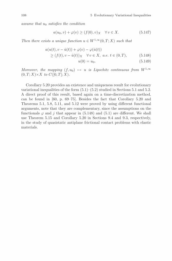
108 5 Evolutionary Variational Inequalities
assume that u0 satisfies the condition
a(u0, v) + ϕ(v) ≥ (f(0), v)X ∀ v ∈ X. (5.147)
Then there exists a unique function u ∈ W 1,∞(0, T ;X) such that
a(u(t), v − u(t)) + ϕ(v) − ϕ(u(t))
≥ (f(t), v − u(t))X ∀ v ∈ X, a.e. t ∈ (0, T ), (5.148)
u(0) = u0. (5.149)
Moreover, the mapping (f, u0) → u is Lipschitz continuous from W 1,∞
(0, T ;X)×X to C([0, T ];X).
Corollary 5.20 provides an existence and uniqueness result for evolutionaryvariational inequalities of the form (5.1)–(5.2) studied in Sections 5.1 and 5.2.A direct proof of this result, based again on a time-discretization method,can be found in [60, p. 69–75]. Besides the fact that Corollary 5.20 andTheorems 5.1, 5.8, 5.11, and 5.12 were proved by using different functionalarguments, note that they are complementary, since the assumptions on thefunctionals ϕ and j that appear in (5.148) and (5.1) are different. We shalluse Theorem 5.15 and Corollary 5.20 in Sections 9.4 and 9.3, respectively,in the study of quasistatic antiplane frictional contact problems with elasticmaterials.

Chapter 6
Volterra-type Variational Inequalities
The variational inequalities studied in this chapter involve the Volterraoperator, (4.42), and therefore are history dependent. The term containingthis operator appears as a perturbation of the bilinear form a and it is notinvolved in the function j; even if various other cases may be considered, wemade this choice since it is suggested by the structure of variational mod-els that describe the frictional contact of viscoelastic materials with longmemory. We consider two types of variational inequalities with a Volterraintegral term: the first one is elliptic, and the second one is evolutionary. Forboth inequalities, we provide existence and uniqueness results. Finally, westudy the behavior of the solution with respect to the integral term and withrespect to the nondifferentiable function and provide convergence results. Theresults presented in this chapter will be applied in the study of antiplane fric-tional contact problems involving viscoelastic materials with long memory.Everywhere in this chapter, X is a real Hilbert space with the inner product(·, ·)X , and the norm ‖ · ‖X , and [0, T ] denotes the time interval of interest,where T > 0.
6.1 Volterra-type Elliptic Variational Inequalities
In this section, we consider the problem of finding u : [0, T ] → X such that
a(u(t), v − u(t)) +
(∫ t
0
A(t − s) u(s) ds, v − u(t)
)
X
+ j(v) − j(u(t))
≥ (f(t), v − u(t))X ∀ v ∈ X, t ∈ [0, T ], (6.1)
where a is a bilinear form on X, j : X → (−∞, ∞], A : [0, T ] → L(X)and f : [0, T ] → X. Note that problem (6.1) does not involve the timederivative of the unknown u and, therefore, it represents an elliptic variationalinequality; moreover, since this problem involves the Volterra operator (4.42)
109

110 6 Volterra-type Variational Inequalities
with Y = X and y0 = 0X , we refer to it as a Volterra-type elliptic variationalinequality.
In the study of (6.1) we assume that:
a : X × X → R is a bilinear symmetric form and
(a) there exists M > 0 such that|a(u, v)| ≤ M‖u‖X ‖v‖X ∀u, v ∈ X.
(b) there exists m > 0 such thata(v, v) ≥ m ‖v‖2
X ∀ v ∈ X.
(6.2)
A ∈ C([0, T ];L(X)). (6.3)
j : X → (−∞,∞] is a proper convex l.s.c. function. (6.4)
f ∈ C([0, T ];X). (6.5)
The main result of this section is the following.
Theorem 6.1. Let X be a Hilbert space and assume that (6.2)–(6.5) hold.Then there exists a unique solution u to problem (6.1). Moreover, the solutionsatisfies u ∈ C([0, T ];X).
Proof. The proof will be carried out in several steps, and it is based on theresults on time-dependent elliptic variational inequalities presented in Sec-tion 3.4 and a fixed point argument. The steps of the proof are the following.
(i) Let η ∈ C([0, T ];X). We use Theorem 3.12 to see that there exists aunique function uη ∈ C([0, T ];X) such that
a(uη(t), v − uη(t)) + (η(t), v − uη(t))X + j(v) − j(uη(t))
≥ (f(t), v − uη(t))X ∀ v ∈ X, t ∈ [0, T ]. (6.6)
(ii) Next, we consider the operator Λ : C([0, T ];X) → C([0, T ];X)given by
Λη(t) =
∫ t
0
A(t − s) uη(s) ds ∀ η ∈ C([0, T ];X), t ∈ [0, T ] (6.7)
and we note that by condition (6.3), the integral in (6.7) is well-defined andthe operator Λ takes values in the space C([0, T ];X).
We prove now that Λ has a unique fixed point η∗ ∈ C([0, T ];X). To thisend, consider two elements η1, η2 ∈ C([0, T ];X), denote u1 = uη1
, u2 = uη2,
and let t ∈ [0, T ]. Using (6.7), we find that
‖Λη1(t) − Λη2(t)‖X ≤∫ t
0
‖A(t − s)‖L(X)‖u1(s) − u2(s)‖X ds
and, keeping in mind (6.3), it follows that
‖Λη1(t) − Λη2(t)‖X ≤ c
∫ t
0
‖u1(s) − u2(s)‖X ds (6.8)

6.1 Volterra-type Elliptic Variational Inequalities 111
where c = ‖A‖C([0,T ];L(X)). Moreover, by using (6.6), after some algebraicmanipulations we find that, for all s ∈ [0, T ], the following inequality holds:
a(u1(s) − u2(s), u1(s) − u2(s)) ≤ (η1(s) − η2(s), u2(s) − u1(s))X .
Therefore, using the X-ellipticity of a, (6.2)(b), we deduce that
‖u1(s) − u2(s)‖X ≤ 1
m‖η1(s) − η2(s)‖X ∀ s ∈ [0, T ]. (6.9)
We combine (6.8) and (6.9) to see that
‖Λη1(t) − Λη2(t)‖X ≤ c
m
∫ t
0
‖η1(s) − η2(s)‖X ds
and then use Lemma 1.42 to conclude this step.
(iii) Existence. Let η∗ ∈ C([0, T ];X) be the fixed point of Λ and let uη∗
be the function defined by (6.6) for η = η∗. Since Λη∗ = η∗, it follows by(6.6), (6.7) that uη∗ satisfies (6.1) and, moreover, uη∗ ∈ C([0, T ];X).
(iv) Uniqueness. The uniqueness is a consequence of the uniqueness ofthe fixed point of the operator Λ. A direct proof can be obtained as follows:let u1, u2 ∈ C([0, T ];X) be two functions that satisfy (6.1) and let t ∈ [0, T ].Then, after some algebra it follows that
a(u1(t)−u2(t), u1(t)−u2(t)) ≤(∫ t
0
A(t−s)(u1(s)−u2(s))ds, u2(t)−u1(t)
)
X
and using assumptions (6.2) and (6.3) yields
‖u1(t) − u2(t)‖X ≤ c
m
∫ t
0
‖u1(s) − u2(s)‖X ds (6.10)
where, again, c = ‖A‖C([0,T ];L(X)). It follows from (6.10) and Lemma 1.44that u1(t) = u2(t), which concludes the proof. ⊓⊔
Applying Theorem 6.1 to the case when j is the indicator function of anonempty, convex, and closed subset K ⊂ X leads to the following result.
Corollary 6.2. Let X be a Hilbert space, let K ⊂ X be a nonempty, convex,and closed subset, and assume that (6.2), (6.3), (6.5) hold. Then there existsa unique function u ∈ C([0, T ];X) such that
u(t) ∈ K, a(u(t), v − u(t)) +
(∫ t
0
A(t − s) u(s) ds, v − u(t)
)
X
≥ (f(t), v − u(t))X ∀ v ∈ K, t ∈ [0, T ].
We end this section with the following regularity result.

112 6 Volterra-type Variational Inequalities
Theorem 6.3. Under the conditions stated in Theorem 6.1, if there existsp ∈ [1, ∞] such that f ∈ W 1,p(0, T ;X) and A ∈ W 1,p(0, T ;L(X)), thenu ∈ W 1,p(0, T ;X).
Proof. Denote
η(t) =
∫ t
0
A(t − s)u(s) ds ∀ t ∈ [0, T ]. (6.11)
It follows that η is differentiable almost everywhere on (0, T ) and, moreover,
η(t) = A(0)u(t) +
∫ t
0
A(t − s)u(s) ds a.e. t ∈ (0, T ).
Now, since A ∈ W 1,p(0, T ;L(X)), we deduce that η ∈ Lp(0, T ;X), i.e.,η ∈ W 1,p(0, T ;X). We use now (6.1) and (6.11) to see that
a(u(t), v − u(t)) + j(v) − j(u(t))
≥ (f(t) − η(t), v − u(t))X ∀ v ∈ X, t ∈ [0, T ].
Since f − η ∈ W 1,p(0, T ;X), it follows from Theorem 3.12 that u ∈W 1,p(0, T ;X), which concludes the proof. ⊓⊔
6.2 Volterra-type Evolutionary Variational Inequalities
In this section, we study the evolutionary version of inequality (6.1), whichcan be formulated as follows: find u : [0, T ] → X such that
a(u(t), v − u(t)) +
(∫ t
0
A(t − s) u(s) ds, v − u(t)
)
X
+ j(v) − j(u(t))
≥ (f(t), v − u(t))X ∀ v ∈ X, a.e. t ∈ (0, T ), (6.12)
u(0) = u0. (6.13)
In the study of this problem, we assume that the bilinear form a satisfiescondition (6.2), the function j satisfies condition (6.4), and, moreover,
A ∈ W 1,2(0, T ;L(X)), (6.14)
f ∈ W 1,2(0, T ;X), (6.15)
u0 ∈ X, (6.16)
There exists δ0 ≥ 0 such thata(u0, v) + j(v) ≥ (f(0), v)X − δ0 ∀ v ∈ X.
(6.17)

6.2 Volterra-type Evolutionary Variational Inequalities 113
Note that condition (6.17) represents a compatibility condition for the ini-tial data of problem (6.12)–(6.13), identical to condition (5.7) used in Chap-ter 5, in the study of evolutionary variational inequalities. The use of thiscondition in the study of Volterra-type evolutionary variational inequalitiesis not surprising, since (6.12)–(6.13) and (5.1)–(5.2) have a common feature,(6.12)–(6.13) being a perturbation of (5.1)–(5.2) with an integral term.
The main result of this section is the following.
Theorem 6.4. Let X be a Hilbert space and assume that (6.2), (6.4), (6.14)–(6.17) hold. Then there exists a unique solution u to problem (6.12)–(6.13).Moreover, the solution satisfies u ∈ W 1,2(0, T ;X).
The proof of Theorem 6.4 will be carried out in several steps and is basedon Theorem 5.12 and a fixed point argument. We assume in what followsthat (6.2), (6.4), (6.14)–(6.17) hold and we introduce the set
W = η ∈ W 1,2(0, T ;X) | η(0) = 0X. (6.18)
The first step is the following.
Lemma 6.5. For each η ∈ W, there exists a unique uη ∈ W 1,2(0, T ;X)such that
a(uη(t), v − uη(t)) + (η(t), v − uη(t))X + j(v) − j(uη(t))
≥ (f(t), v − uη(t))X ∀ v ∈ X, a.e. t ∈ (0, T ), (6.19)
uη(0) = u0. (6.20)
Lemma 6.5 is a simple consequence of Theorem 5.12. It also can be obtai-ned from Theorem 5.1 if the function j satisfies assumption (5.4), as well asby Theorem 5.11 if (5.63) holds and there exists a family of functionals jρthat satisfies (5.64) and (3.17).
In the next step, we consider the operator Λ : W → W defined by
Λη(t) =
∫ t
0
A(t − s)uη(s) ds, ∀ η ∈ W, t ∈ [0, T ]. (6.21)
Keeping in mind assumption (6.14), it is easy to check that if η ∈ W, thenΛη ∈ W and therefore the operator Λ is well defined. A standard computationshows that(
d
dtΛη
)(t) = A(0)uη(t) +
∫ t
0
A(t − s)uη(s) ds ∀ η ∈ W, a.e. t ∈ (0, T ).
(6.22)
We have the following result.
Lemma 6.6. The operator Λ has a unique fixed point η∗ ∈ W.
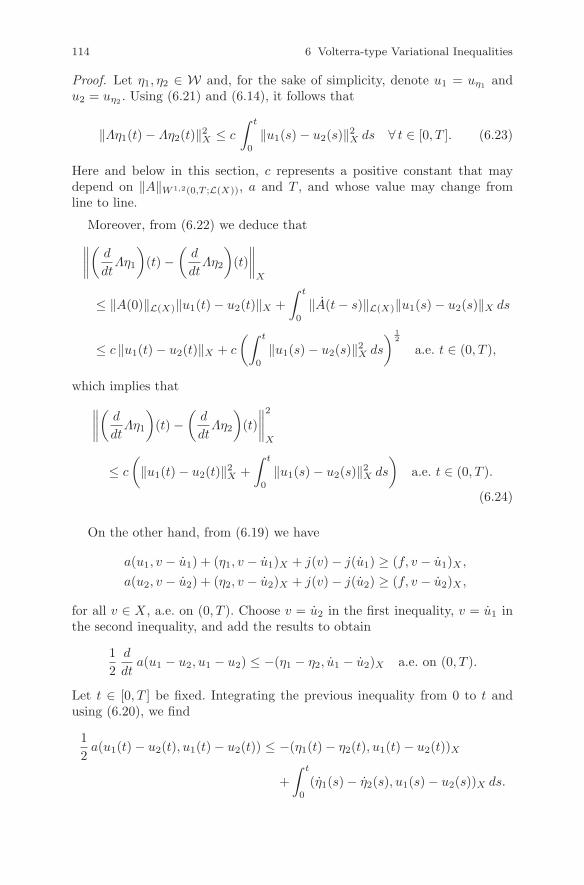
114 6 Volterra-type Variational Inequalities
Proof. Let η1, η2 ∈ W and, for the sake of simplicity, denote u1 = uη1and
u2 = uη2. Using (6.21) and (6.14), it follows that
‖Λη1(t) − Λη2(t)‖2X ≤ c
∫ t
0
‖u1(s) − u2(s)‖2X ds ∀ t ∈ [0, T ]. (6.23)
Here and below in this section, c represents a positive constant that maydepend on ‖A‖W 1,2(0,T ;L(X)), a and T , and whose value may change fromline to line.
Moreover, from (6.22) we deduce that
∥∥∥∥(
d
dtΛη1
)(t) −
(d
dtΛη2
)(t)
∥∥∥∥X
≤ ‖A(0)‖L(X)‖u1(t) − u2(t)‖X +
∫ t
0
‖A(t − s)‖L(X)‖u1(s) − u2(s)‖X ds
≤ c ‖u1(t) − u2(t)‖X + c
(∫ t
0
‖u1(s) − u2(s)‖2X ds
) 12
a.e. t ∈ (0, T ),
which implies that
∥∥∥∥(
d
dtΛη1
)(t) −
(d
dtΛη2
)(t)
∥∥∥∥2
X
≤ c
(‖u1(t) − u2(t)‖2
X +
∫ t
0
‖u1(s) − u2(s)‖2X ds
)a.e. t ∈ (0, T ).
(6.24)
On the other hand, from (6.19) we have
a(u1, v − u1) + (η1, v − u1)X + j(v) − j(u1) ≥ (f, v − u1)X ,
a(u2, v − u2) + (η2, v − u2)X + j(v) − j(u2) ≥ (f, v − u2)X ,
for all v ∈ X, a.e. on (0, T ). Choose v = u2 in the first inequality, v = u1 inthe second inequality, and add the results to obtain
1
2
d
dta(u1 − u2, u1 − u2) ≤ −(η1 − η2, u1 − u2)X a.e. on (0, T ).
Let t ∈ [0, T ] be fixed. Integrating the previous inequality from 0 to t andusing (6.20), we find
1
2a(u1(t) − u2(t), u1(t) − u2(t)) ≤ −(η1(t) − η2(t), u1(t) − u2(t))X
+
∫ t
0
(η1(s) − η2(s), u1(s) − u2(s))X ds.

6.2 Volterra-type Evolutionary Variational Inequalities 115
It follows now from (6.2) that
m
2‖u1(t) − u2(t)‖2
X ≤ ‖η1(t) − η2(t)‖X‖u1(t) − u2(t)‖X
+
∫ t
0
‖η1(s) − η2(s)‖X‖u1(s) − u2(s)‖X ds
and, using the inequality
ab ≤ a2
2α+ 2αb2 ∀ a, b, α > 0
with a convenient choice of α, we find
‖u1(t) − u2(t)‖2X ≤ c
(‖η1(t) − η2(t)‖2
X +
∫ t
0
‖η1(s) − η2(s)‖2Xds
+
∫ t
0
‖u1(s) − u2(s)‖2X ds
). (6.25)
Now, since
η1(t) − η2(t) =
∫ t
0
(η1(s) − η2(s)) ds,
we deduce that
‖η1(t) − η2(t)‖2X ≤ c
∫ t
0
‖η1(s) − η2(s)‖2X ds.
Substituting this inequality in (6.25), we obtain
‖u1(t) − u2(t)‖2X ≤ c
(∫ t
0
‖η1(s) − η2(s)‖2X ds +
∫ t
0
‖u1(s) − u2(s)‖2X ds
).
Applying now Gronwall’s inequality (Lemma 1.44) yields
‖u1(t) − u2(t)‖2X ≤ c
∫ t
0
‖η1(s) − η2(s)‖2X ds, (6.26)
which implies that
∫ t
0
‖u1(s) − u2(s)‖2X ds ≤ c
∫ t
0
‖η1(s) − η2(s)‖2X ds. (6.27)
We combine (6.23), (6.24), (6.26), and (6.27) to obtain
‖Λη1(t) − Λη2(t)‖2X +
∥∥∥∥(
d
dtΛη1
)(t) −
(d
dtΛη2
)(t)
∥∥∥∥2
X
≤ c
∫ t
0
‖η1(s) − η2(s)‖2X ds.

116 6 Volterra-type Variational Inequalities
Iterating the last inequality, we infer
‖Λmη1(t) − Λmη2(t)‖2X +
∥∥∥∥(
d
dtΛmη1
)(t) −
(d
dtΛmη2
)(t)
∥∥∥∥2
X
≤ cm
∫ t
0
∫ s1
0
· · ·∫ sm−1
0
‖η1(sm) − η2(sm)‖2X dsm · · · ds1,
where Λm denotes the m-th power of the operator Λ. The last inequalityimplies
‖Λmη1 − Λmη2‖2W 1,2(0,T ;X) ≤ cm Tm
m!‖η1 − η2‖2
W 1,2(0,T ;X).
Since limm→∞
cmTm
m!= 0, the previous inequality implies that for m large
enough, a power Λm of Λ is a contraction in W. Lemma 6.6 is now a conse-quence of Theorem 1.41, since W is a closed subspace of the Hilbert spaceW 1,2(0, T ;X). ⊓⊔
We have now all the ingredients needed to prove the theorem.
Proof. Existence. Let η∗ ∈ W be the fixed point of Λ and let uη∗ be thefunction defined by Lemma 6.5 for η = η∗. Since Λη∗ = η∗, it follows from(6.19)–(6.21) that uη∗ is a solution of problem (6.12)–(6.13). Moreover, theregularity uη∗ ∈ W 1,2(0, T ;X) is obtained from Lemma 6.5.
Uniqueness. The uniqueness is a consequence of the uniqueness of the fixedpoint of the operator Λ. Indeed, let u be a solution of problem (6.12)–(6.13)with regularity u ∈ W 1,2(0, T ;X) and consider the element η ∈ W defined by
η(t) =
∫ t
0
A(t − s)u(s) ds ∀ t ∈ [0, T ]. (6.28)
It follows that u is the solution of problem (6.19)–(6.20), and by the unique-ness of this solution (guaranteed by Lemma 6.5) we have
u = uη. (6.29)
We conclude by (6.21), (6.28), and (6.29) that Λη = η; therefore, from theuniqueness of the fixed point of the operator Λ (guaranteed by Lemma 6.6),it follows that
η = η∗. (6.30)
The uniqueness part of Theorem 6.4 is now a consequence of (6.29) and(6.30). ⊓⊔
We end this section with the following result.
Corollary 6.7. Let X be a Hilbert space and let K ⊂ X be a nonempty, con-vex, and closed subset. Assume that (6.2), (6.14)–(6.16) hold and, moreover,

6.3 Convergence Results 117
there exists δ0 ≥ 0 such that a(u0, v) ≥ (f(0), v)X − δ0 for all v ∈ K. Thenthere exists a unique function u ∈ W 1,2(0, T ;X) such that u(0) = u0 and
u(t) ∈ K, a(u(t), v − u(t)) +
(∫ t
0
A(t − s) u(s) ds, v − u(t)
)
X
≥ (f(t), v − u(t))X ∀ v ∈ K, a.e. t ∈ (0, T ).
Corollary 6.7 is a direct consequence of Theorem 6.4 and is obtained bychoosing j = ψK , where ψK represents the indicator function of the set K.
6.3 Convergence Results
In this section, we study the dependence of the solution of the Volterra-typevariational inequalities on the operator A and on the function j, as well.
We start with the case of elliptic variational inequalities. To this end, weassume in what follows that (6.2)–(6.5) hold and we denote by u ∈ C([0, T ];X)the solution of (6.1) obtained in Theorem 6.1. Let Θ be a given set of param-eters and, for every θ ∈ Θ, denote by Aθ a perturbation of A that satisfies
Aθ ∈ C([0, T ];L(X)). (6.31)
Also, consider the problem of finding uθ : [0, T ] → X such that
a(uθ(t), v − uθ(t)) +
(∫ t
0
Aθ(t − s) uθ(s) ds, v − uθ(t)
)
X
+ j(v) − j(uθ(t))
≥ (f(t), v − uθ(t))X ∀ v ∈ X, t ∈ [0, T ]. (6.32)
We deduce from Theorem 6.1 that the variational inequality (6.32) hasa unique solution uθ ∈ C([0, T ];X), for every θ ∈ Θ. Consider now theassumption
‖Aθ − A‖C([0,T ];L(X)) → 0. (6.33)
We have the following convergence result.
Theorem 6.8. Assume that (6.2)–(6.5), (6.31), and (6.33) hold. Then thesolution uθ of problem (6.32) converges to the solution u of problem (6.1), i.e.,
‖uθ − u‖C([0,T ];X) → 0. (6.34)
Note that the convergence result presented in Theorem 6.8 is understoodin the following sense, already described on pages 48 and 95: for everysequence θn ⊂ Θ such that ‖Aθn
− A‖C([0,T ];L(X)) → 0 as n → ∞, one has‖uθn
− u‖C([0,T ];X) → 0 as n → ∞.

118 6 Volterra-type Variational Inequalities
Proof. Let θ ∈ Θ. Everywhere below c will represent a positive constant thatmay depend on a, A, u, and T , but is independent of t and θ, and whosevalue may change from place to place. Denote
ηθ(t) =
∫ t
0
Aθ(t − s) uθ(s) ds ∀ t ∈ [0, T ], (6.35)
η(t) =
∫ t
0
A(t − s) u(s) ds ∀ t ∈ [0, T ]. (6.36)
We use (6.32) and (6.1) to obtain
a(uθ(t), v −uθ(t)) + (ηθ(t), v −uθ(t))X + j(v) − j(uθ(t)) ≥ (f(t), v −uθ(t))X ,
a(u(t), v − u(t)) + (η(t), v − u(t))X + j(v) − j(u(t)) ≥ (f(t), v − u(t))X ,
for all v ∈ X and t ∈ [0, T ], and using arguments similar to those in the proofof (6.9) yields
‖uθ(t) − u(t)‖X ≤ c ‖ηθ(t) − η(t)‖X ∀t ∈ [0, T ]. (6.37)
It follows from (6.35) and (6.36) that
‖ηθ(t) − η(t)‖X ≤∫ t
0
‖Aθ(t − s)uθ(s) − A(t − s)u(s)‖X ds
≤∫ t
0
‖Aθ(t − s)‖L(X)‖uθ(s) − u(s)‖X ds
+
∫ t
0
‖Aθ(t − s) − A(t − s)‖L(X)‖u(s)‖X ds ∀ t ∈ [0, T ].
So,
‖ηθ(t) − η(t)‖X ≤ ‖Aθ‖C([0,T ];L(X))
∫ t
0
‖uθ(s) − u(s)‖X ds
+ c ‖Aθ − A‖C([0,T ];L(X)) ∀ t ∈ [0, T ]. (6.38)
As θ → 0, it follows from (6.33) that there exists c > 0 such that
‖Aθ‖C([0,T ];L(X)) ≤ c. (6.39)
We combine (6.37), (6.38), and (6.39) to obtain
‖uθ(t) − u(t)‖X ≤ c
(∫ t
0
‖uθ(s) − u(s)‖X ds + ‖Aθ − A‖C([0,T ];L(X))
)
for all t ∈ [0, T ], and using Gronwall’s inequality (Lemma 1.44), we find that
‖uθ(t) − u(t)‖X ≤ c ‖Aθ − A‖C([0,T ];L(X)) ∀ t ∈ [0, T ]. (6.40)
The convergence result (6.34) is now a consequence of (6.33) and (6.40). ⊓⊔
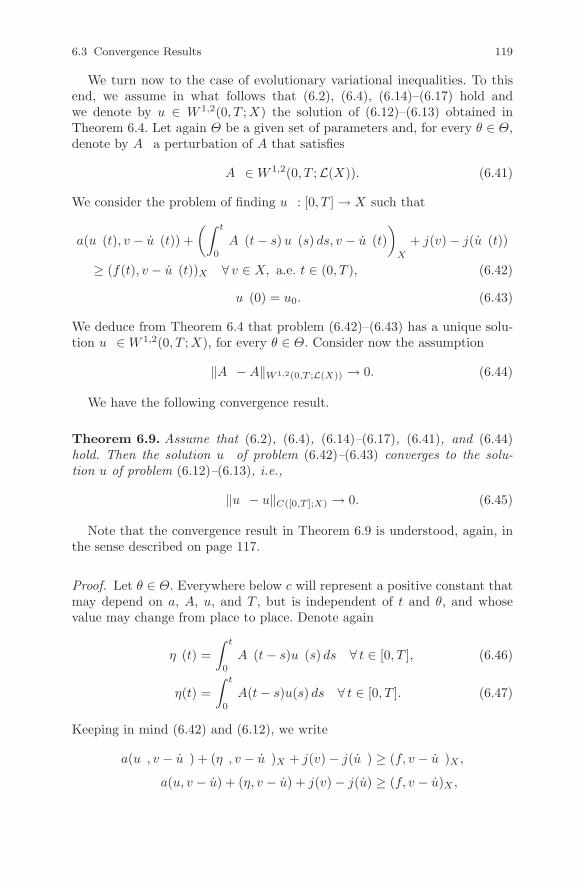
6.3 Convergence Results 119
We turn now to the case of evolutionary variational inequalities. To thisend, we assume in what follows that (6.2), (6.4), (6.14)–(6.17) hold andwe denote by u ∈ W 1,2(0, T ;X) the solution of (6.12)–(6.13) obtained inTheorem 6.4. Let again Θ be a given set of parameters and, for every θ ∈ Θ,denote by Aθ a perturbation of A that satisfies
Aθ ∈ W 1,2(0, T ;L(X)). (6.41)
We consider the problem of finding uθ : [0, T ] → X such that
a(uθ(t), v − uθ(t)) +
(∫ t
0
Aθ(t − s) uθ(s) ds, v − uθ(t)
)
X
+ j(v) − j(uθ(t))
≥ (f(t), v − uθ(t))X ∀ v ∈ X, a.e. t ∈ (0, T ), (6.42)
uθ(0) = u0. (6.43)
We deduce from Theorem 6.4 that problem (6.42)–(6.43) has a unique solu-tion uθ ∈ W 1,2(0, T ;X), for every θ ∈ Θ. Consider now the assumption
‖Aθ − A‖W 1,2(0,T ;L(X)) → 0. (6.44)
We have the following convergence result.
Theorem 6.9. Assume that (6.2), (6.4), (6.14)–(6.17), (6.41), and (6.44)hold. Then the solution uθ of problem (6.42)–(6.43) converges to the solu-tion u of problem (6.12)–(6.13), i.e.,
‖uθ − u‖C([0,T ];X) → 0. (6.45)
Note that the convergence result in Theorem 6.9 is understood, again, inthe sense described on page 117.
Proof. Let θ ∈ Θ. Everywhere below c will represent a positive constant thatmay depend on a, A, u, and T , but is independent of t and θ, and whosevalue may change from place to place. Denote again
ηθ(t) =
∫ t
0
Aθ(t − s)uθ(s) ds ∀ t ∈ [0, T ], (6.46)
η(t) =
∫ t
0
A(t − s)u(s) ds ∀ t ∈ [0, T ]. (6.47)
Keeping in mind (6.42) and (6.12), we write
a(uθ, v − uθ) + (ηθ, v − uθ)X + j(v) − j(uθ) ≥ (f, v − uθ)X ,
a(u, v − u) + (η, v − u) + j(v) − j(u) ≥ (f, v − u)X ,

120 6 Volterra-type Variational Inequalities
for all v ∈ X, a.e. on (0, T ), and using arguments similar to those used in theproof of (6.26) yields
‖uθ(t) − u(t)‖2X ≤ c
∫ t
0
‖ηθ(s) − η(s)‖2Xds ∀ t ∈ [0, T ]. (6.48)
It follows now from (6.46) and (6.47) that
ηθ(t) = Aθ(0)uθ(t) +
∫ t
0
Aθ(t − s)uθ(s) ds,
η(t) = A(0)u(t) +
∫ t
0
A(t − s)u(s) ds,
a.e. t ∈ (0, T ), which imply
‖ηθ(t) − η(t)‖X ≤ ‖Aθ(0)‖L(X)‖uθ(t) − u(t)‖X + ‖Aθ(0)−A(0)‖L(X)‖u(t)‖X
+
∫ t
0
‖Aθ(t − s)‖L(X)‖uθ(s) − u(s)‖X ds
+
∫ t
0
‖Aθ(t − s) − A(t − s)‖L(X)‖u(s)‖X ds, (6.49)
a.e. t ∈ (0, T ). As θ → 0, it follows from (6.44) that there exists c > 0such that
‖Aθ‖C([0,T ];L(X)) ≤ c, ‖Aθ‖L2(0,T ;L(X)) ≤ c.
Using now these inequalities in (6.49) will yield after some algebra
‖ηθ(t) − η(t)‖2X
≤ c
(‖Aθ − A‖2
W 1,2(0,T ;L(X)) + ‖uθ(t) − u(t)‖2X +
∫ t
0
‖uθ(s) − u(s)‖2Xds
),
a.e. t ∈ (0, T ). The previous inequality implies∫ t
0
‖ηθ(s) − η(s)‖2X ds
≤ c
(‖Aθ − A‖2
W 1,2(0,T ;L(X)) +
∫ t
0
‖uθ(s) − u(s)‖2X ds
)∀ t ∈ [0, T ].
(6.50)
We combine now (6.48) and (6.50) to obtain
‖uθ(t) − u(t)‖2X ≤ c
(‖Aθ − A‖2
W 1,2(0,T ;L(X)) +
∫ t
0
‖uθ(s) − u(s)‖2X ds
)
for all t ∈ [0, T ] and, using again Gronwall’s inequality, we find
‖uθ(t) − u(t)‖X ≤ c ‖Aθ − A‖W 1,2(0,T ;L(X)) ∀ t ∈ [0, T ]. (6.51)
The convergence (6.45) is now a consequence of (6.44) and (6.51). ⊓⊔

6.3 Convergence Results 121
We now continue with the study of the dependence of the solution of thevariational inequality (6.1) on the function j. To this end, we assume in whatfollows that (6.2)–(6.5) hold and, again, we denote by u ∈ C([0, T ];X) thesolution of (6.1) obtained in Theorem 6.1. Also, for every ρ > 0, denote byjρ a perturbation of j that satisfies (6.4), i.e.,
jρ : X → (−∞,∞] is a proper convex l.s.c. function. (6.52)
It follows from Theorem 6.1 that there exists a unique function uρ ∈C([0, T ];X) such that
a(uρ(t), v − uρ(t)) +
(∫ t
0
A(t − s)uρ(s) ds, v − uρ(t)
)
X
+ jρ(v) − jρ(uρ(t))
≥ (f(t), v − uρ(t))X ∀ v ∈ X, t ∈ [0, T ]. (6.53)
The behavior of the solution uρ as ρ → 0 is given by the following theorem.
Theorem 6.10. Assume that (6.2)–(6.5), (6.52), and (3.17) hold. Then thesolution uρ of problem (6.53) converges to the solution u of problem(6.1), i.e.,
‖uρ − u‖C([0,T ];X) → 0 as ρ → 0. (6.54)
Proof. Let ρ > 0 and t ∈ [0, T ]. Everywhere below c will represent a positiveconstant that may depend on a, A, u, and T , but it is independent on t and ρ,and whose value may change from place to place.
We choose v = uρ(t) in (6.1) and v = u(t) in (6.53) and add the resultinginequalities to obtain
a(uρ(t) − u(t), uρ(t) − u(t))
≤(∫ t
0
A(t − s)(u(s) − uρ(s)) ds, uρ(t) − u(t)
)
X
+ j(uρ(t)) − j(u(t)) + jρ(u(t)) − jρ(uρ(t)). (6.55)
Assumption (6.3) on A implies
(∫ t
0
A(t − s) (u(s) − uρ(s)) ds, uρ(t) − u(t)
)
X
≤(∫ t
0
‖A(t − s)‖L(X)‖uρ(s) − u(s)‖X ds
)‖uρ(t) − u(t)‖X
≤ c
(∫ t
0
‖uρ(s) − u(s)‖X ds
)‖uρ(t) − u(t)‖X

122 6 Volterra-type Variational Inequalities
and, using the elementary inequality
c ab ≤ c2
2ma2 +
m
2b2,
we find that(∫ t
0
A(t − s) (u(s) − uρ(s)) ds, uρ(t) − u(t)
)
X
≤ c2
2m
(∫ t
0
‖uρ(s) − u(s)‖X ds
)2
+m
2‖uρ(t) − u(t)‖2
X . (6.56)
On the other hand, assumption (3.17)(a) on jρ leads to
j(uρ(t)) − j(u(t)) + jρ(u(t)) − jρ(uρ(t)) ≤ 2 F (ρ). (6.57)
We combine now inequalities (6.55)–(6.57) and use the X-ellipticity of theform a, (6.2)(b), to obtain
m
2‖uρ(t) − u(t)‖2
X ≤ c2
2m
(∫ t
0
‖uρ(s) − u(s)‖X ds
)2
+ 2 F (ρ)
which yields
‖uρ(t) − u(t)‖2X ≤ c
(∫ t
0
‖uρ(s) − u(s)‖2Xds + F (ρ)
). (6.58)
The Gronwall argument in (6.58) implies that
‖uρ(t) − u(t)‖X ≤ c√
F (ρ). (6.59)
The convergence result (6.54) is now a consequence of inequality (6.59) com-bined with assumption (3.17)(b). ⊓⊔
A convergence result similar to that in Theorem 6.10 can be obtained in thestudy of the evolutionary variational inequality (6.12)–(6.13). To present it,we assume in what follows that (6.2), (6.4), (6.14)–(6.17) hold and we denoteby u ∈ W 1,2(0, T ;X) the solution of (6.12)–(6.13) obtained in Theorem 6.4.Also, for every ρ > 0, denote by jρ a perturbation of j that satisfies (6.52)and (3.17). It follows from the proof of Lemma 5.10 that
a(u0, v) + jρ(v) − (f(0), v)X ≥ −δ0 − F (ρ) ∀ v ∈ X
and, therefore, by using again Theorem 6.4, we obtain that there exists aunique function uρ ∈ W 1,2(0, T ;X) such that
a(uρ(t), v − uρ(t)) +
(∫ t
0
A(t − s) uρ(s) ds, v − uρ(t)
)
X
+ jρ(v) − jρ(uρ(t))
≥ (f(t), v − uρ(t))X ∀ v ∈ X, a.e. t ∈ (0, T ), (6.60)
uρ(0) = u0. (6.61)
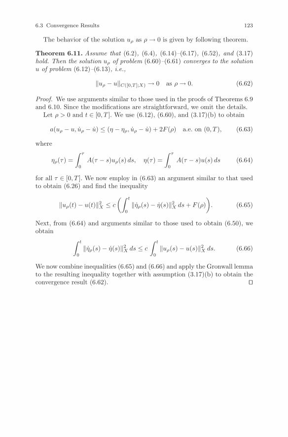
6.3 Convergence Results 123
The behavior of the solution uρ as ρ → 0 is given by following theorem.
Theorem 6.11. Assume that (6.2), (6.4), (6.14)–(6.17), (6.52), and (3.17)hold. Then the solution uρ of problem (6.60)–(6.61) converges to the solutionu of problem (6.12)–(6.13), i.e.,
‖uρ − u‖C([0,T ];X) → 0 as ρ → 0. (6.62)
Proof. We use arguments similar to those used in the proofs of Theorems 6.9and 6.10. Since the modifications are straightforward, we omit the details.
Let ρ > 0 and t ∈ [0, T ]. We use (6.12), (6.60), and (3.17)(b) to obtain
a(uρ − u, uρ − u) ≤ (η − ηρ, uρ − u) + 2F (ρ) a.e. on (0, T ), (6.63)
where
ηρ(τ) =
∫ τ
0
A(τ − s)uρ(s) ds, η(τ) =
∫ τ
0
A(τ − s)u(s) ds (6.64)
for all τ ∈ [0, T ]. We now employ in (6.63) an argument similar to that usedto obtain (6.26) and find the inequality
‖uρ(t) − u(t)‖2X ≤ c
(∫ t
0
‖ηρ(s) − η(s)‖2X ds + F (ρ)
). (6.65)
Next, from (6.64) and arguments similar to those used to obtain (6.50), weobtain
∫ t
0
‖ηρ(s) − η(s)‖2X ds ≤ c
∫ t
0
‖uρ(s) − u(s)‖2X ds. (6.66)
We now combine inequalities (6.65) and (6.66) and apply the Gronwall lemmato the resulting inequality together with assumption (3.17)(b) to obtain theconvergence result (6.62). ⊓⊔

Bibliographical Notes
Interest in variational inequalities originates in mechanical problems, see forinstance [42], where many problems in mechanics and physics are formu-lated in the framework of variational inequalities. More recent referencesin the mathematical analysis of variational inequalities and nonlinear par-tial differential equations include [9, 12, 39, 46, 49, 85, 87, 113]. Detailsconcerning the numerical analysis of variational inequalities can be foundin [52, 53, 61, 67, 86]. A reference in the study of mathematical and numeri-cal analysis of variational inequalities arising in hardening plasticity is [57].
The results presented in Section 3.1 are standard and can be found in manybooks and surveys. In the proof of Theorem 3.1, we followed arguments thatcan be found in [44, 85]. A different proof of Theorem 3.1 can be obtained fol-lowing the ideas in [15]; there, the main ingredients in the proof are the prop-erties of the proximity maps, introduced in [105], and the Banach fixed pointtheorem. Section 3.2 was written following results that can be found in [53,Ch. 1]. The proof of Theorem 3.7, based on the Banach fixed point argument,follows [28]; there, a more general existence and uniqueness result for ellipticquasivariational inequalities involving strongly monotone Lipschitz continu-ous operators is presented. Theorem 3.10 represents a simplified version of amore general result on elliptic quasivariational inequalities obtained in [107].There, the existence of the solution was proved by using the properties ofthe directional derivative of the function j and topological degree arguments;moreover, an application in the study of a static problem modeling the fric-tional contact with normal compliance and Coulomb’s law was considered.
The results presented in Sections 4.1 and 4.3 in the study of evolution-ary variational inequalities with viscosity are based on more general resultsderived in [58, 59], see also [8]. In [58, 59], the unique solvability of vari-ational inequalities of the form (4.29)–(4.30) and (4.31)–(4.32) was provedtogether with their numerical analysis, based on the study of semidiscreteand fully discrete schemes. Error estimates and convergence results were alsoobtained. Moreover, applications in the study of three-dimensional frictionalcontact problems with normal compliance and normal damped response were
125

126 Bibliographical Notes
provided. The results in Sections 4.2 and 4.4 represent abstract versions ofthe results obtained in [3, 24, 122, 129] in the study of variational inequali-ties modeling quasistatic frictional contact problems involving Kelvin-Voigtviscoelastic materials. A survey of these results can be found in [60]. There,the existence and uniqueness of the weak solution for various viscoelastic andviscoplastic contact problems is proved, fully discrete numerical schemes areproposed and implemented, and the results of the corresponding numericalsimulations are presented.
Evolutionary variational inequalities of the form (5.1)–(5.2) have beenstudied by many authors, under various assumptions on the function j, see,e.g., [16, 37, 57, 60]. The results in [16] are based on arguments of nonlinearequations with maximal monotone operators. The results in [57] and [60] usea time discretization method, under the assumption that j is a positivelyhomogeneous function or a seminorm, respectively. The time discretizationmethod in the study of evolutionary variational inequalities arising in con-tact mechanics was also used in [2, 4, 29, 30, 31, 32]. In writing Sections 5.1and 5.2, we used some ideas of [37]. There, evolutionary variational inequal-ities of the form (5.1)–(5.2) were considered in the case when the func-tion j is time-dependent and the existence of the solution was proved byusing a regularization method involving Gateaux differentiable functions.Note also that a regularization method similar to that used in Section 5.2was used in [42] in the study of parabolic evolutionary variational inequalities.A convergence result similar to that presented in Theorem 5.14 was obtainedin [132], in the study of evolutionary variational inequalities with viscosityinvolving strongly monotone Lipschitz continuous operators. Section 5.4 waswritten following [106]. There, Theorem 5.15 was presented in the more gen-eral case when j is a subadditive and positively homogeneous functional; also,an application to the study of a quasistatic frictional contact problem withnormal compliance for linearly elastic materials was considered.
Most of the results presented in Chapter 6 of this book are based on ourresearch and were obtained in [123, 136]. Thus, Volterra-type elliptic varia-tional inequalities of the form (6.1) were studied in [123] where the proof ofTheorem 6.1 was obtained; the numerical approximation of the problem wasalso considered, based on spatially semidiscrete and fully discrete schemes,and error estimates were derived; the abstract results were then used in thestudy of the Signorini frictionless contact problem between two viscoelas-tic bodies with long memory. The study of evolutionary variational inequal-ity (6.12)–(6.13) was performed in [136]; there, Theorems 6.4 and 6.9 wereproved and then used in the study of a frictional contact problem for lin-early viscoelastic materials with long memory; the numerical analysis of thecorresponding frictional contact problem was performed in [124, 125].

Chapter 7
Modeling of Contact Processes
In this chapter, we present a general description of mathematical modeling ofthe processes involved in contact between a deformable body and an obstacleor a foundation. Such kind of processes abound in industry and everyday lifeand, for this reason, a considerable effort has been made in their modeling,analysis, and numerical simulations. We present the physical setting, thevariables that determine the state of the system, the material behavior thatis reflected in a constitutive law, the input data, the equation of evolution forthe state of the system, and the boundary conditions for the system variables.In particular, we provide a description of the frictional contact conditions,including versions of the Coulomb law of dry friction and its regularizations.Most of the notions and results we present here are standard and can be foundin many books on mechanics and, therefore, we skip many of the details. Inthis chapter, all variables are assumed to have sufficient degree of smoothnessconsistent with developments they are involved in.
7.1 Physical Setting
A large variety of situations involving contact phenomena can be cast in thegeneral physical setting shown in Figure 7.1 and described in what follows. Adeformable body occupies, in the reference configuration, an open boundedconnected set B ⊂ R
3 with boundary ∂B. We denote vectors and tensors byboldface letters, such us the position vector x = (xi) ∈ B ∪ ∂B. Here andbelow, the indices i, j, k, l run from 1 to 3; an index that follows a commaindicates a derivative with respect to the corresponding component of thespatial variable x, and the summation convention over repeated indices isadopted. We denote by S
3 the space of second-order symmetric tensors on R3
or, equivalently, the space of symmetric matrices of order 3. The canonical
129

130 7 Modeling of Contact Processes
ΓΓ
Γ
DF
C
B
Fig. 7.1 A deformable body in contact with a foundation.
inner products and the corresponding norms on R3 and S
3 are
u · v = uivi, ‖v‖ = (v · v)1/2 ∀u,v ∈ R3,
σ · τ = σijτij , ‖τ‖ = (τ · τ )1/2 ∀σ, τ ∈ S3,
respectively.
The boundary ∂B is assumed to be composed of three sets ΓD, ΓF , andΓC , with mutually disjoint relatively open sets ΓD, ΓF , and ΓC . We assumethe boundary ∂B is Lipschitz continuous and therefore the unit outwardnormal vector ν exists a.e. on ∂B. The body is clamped on ΓD. Surfacetractions of density f2 act on ΓF and volume forces of density f0 act in B.The body is in contact on ΓC with an obstacle, the so-called foundation. Theforce densities f0 and f2 may depend on time. As a result, the mechanicalstate of the body evolves on the time interval [0, T ], where T > 0.
We are interested in providing a mathematical model that describes theevolution of the body in this physical setting. To this end, we denote byσ = σ(x, t) = (σij(x, t)) the stress field and by u = u(x, t) = (ui(x, t)) thedisplacement field. The functions u : B × [0, T ] → R
3 and σ : B × [0, T ] → S3
will play the role of the unknowns of the contact problem. From time to time,we suppress the explicit dependence of the quantities on the spatial variablex, or both x and t; i.e., when it is convenient to do so, we write σ(t) andu(t), or even σ and u. Also, everywhere below a dot above a variable willrepresent the derivative with respect to time and, therefore, u denotes thevelocity field.
We assume that the volume forces and surface tractions change slowly intime so that the inertia of the mechanical system is negligible. In other words,we neglect the acceleration term in the equation of motion and therefore weconsider a quasistatic process of contact. Thus, the stress field satisfies theequation of equilibrium
Div σ + f0 = 0 in B × (0, T ) (7.1)
where Div is the divergence operator, that is, Div σ = (σij,j), and recall that
σij,j =∂σij
∂xj. Since the body is clamped on ΓD, we impose the displacement

7.1 Physical Setting 131
boundary condition
u = 0 on ΓD × (0, T ). (7.2)
The traction boundary condition is
σν = f2 on ΓF × (0, T ). (7.3)
It states that the stress vector σν is given on part ΓF of the boundary duringthe contact process.
On ΓC we will specify contact conditions. The contact may be frictionlessor frictional, with a rigid or with a deformable foundation and, in the case offrictional contact, a number of different friction conditions may be employed.A survey of the various contact and frictional conditions used in the literaturewill be provided in Sections 7.3–7.5.
We now recall the strain-displacement relation
ε(u) = (εij(u)), εij(u) =1
2(ui,j + uj,i) in B × (0, T ) (7.4)
which defines the infinitesimal strain tensor. Sometimes, we omit the explicitdependence of ε on u by writing ε instead of ε(u). Note that all the problemsstudied in this book are formulated in the framework of small strain theory.
At this stage, the description of our model is not complete: we have moreunknown functions than the number of equations. Indeed, equations (7.1)and (7.4) represent, when written out in their component forms, a total ofnine equations: three from the equilibrium equation and six from strain-displacement relations (taking into account the symmetry of ε). The totalnumber of unknowns is fifteen: three components of the displacement, sixcomponents of the strain, and six components for the stress (again account-ing for the symmetry of ε and σ). Thus, it is clear that six additional equa-tions are required if we are to have a problem that is at least in principlesolvable.
Physical considerations also indicate that the description of the problemso far is incomplete. In addition to the kinematics and the balance lawsthat apply to all the materials, we also need description of the particularmaterial behavior. This information, embodied in the constitutive equationor constitutive law of the material, will provide the remaining equations ofthe problem. A description of the constitutive laws considered in this bookwill be given in Section 7.2. Here we restrict ourselves to remark that in thisbook, we deal only with elastic and viscoelastic materials.
To conclude, the physical setting of the contact problems described aboveis modeled by the system of partial differential equations (7.1), (7.4), supple-mented by the constitutive equation that describes the physical propertiesof the material; the boundary conditions associated to this system are (7.2),(7.3), and the contact condition that is formulated on ΓC × (0, T ); finally,

132 7 Modeling of Contact Processes
if necessary, the system is completed with initial conditions for the displace-ment field or/and the stress field. Note that in the case of static processesfor elastic materials, the data f0 and f2 do not depend on time and, sincethe time variable is not involved in the constitutive law and in the contactboundary conditions, relations (7.1), (7.4) hold in B, and conditions (7.2)and (7.3) hold on ΓD and ΓF , respectively.
7.2 Constitutive Laws
As we noted in Section 7.1, equations (7.1) and (7.4) do not constitute acomplete description of the evolution of a continuous body. To obtain a com-plete model, valid for a given material, we must add the constitutive law ofthe material. Although they must satisfy some basic axioms and invarianceprinciples, constitutive laws originate mostly from experience. A general de-scription of several diagnostic experiments that are made with “standard”universal testing machines can be found in [36, 41, 60]. Below we just presenta description of the elastic and viscoelastic constitutive laws used in thisbook, based on rheological considerations.
In rheology, elastic properties are described by springs, i.e., elements thatprovide a one-to-one connection between the stress σ and the strain ε. A lin-early elastic spring obeys Hooke’s law,
σ = E ε, (7.5)
where the coefficient E > 0 is called the Young modulus. Viscous propertiesare modeled by dashpots, i.e., elements that provide a one-to-one connectionbetween the stress σ and the strain rate ε. A linear dashpot provides a linearrelation between the stress and the strain rate, that is,
σ = η ε. (7.6)
Equation (7.6) is called Newton’s constitutive law, and the coefficient η > 0is called the Newtonian viscosity. Recall that here and below, a dot abovea variable denotes the derivative of that variable with respect to the time.Basic rheological elements are plotted schematically in Figure 7.2.
To proceed with the construction of rheological models, it is natural tocombine these elements in groups. Two possibilities arise in combining theseelements: in series and in parallel. The former leads to the Maxwell model, seeFigure 7.3, whereas the latter leads to the Kelvin-Voigt model, see Figure 7.4.
To obtain more general models, we combine the basic elements (springs anddashpots) as well as the Maxwell and Kelvin-Voigt elements in parallel andseries. For example, taking the Maxwell model together with an elastic springin parallel, we obtain the standard viscoelastic model, see Figure 7.5. By thisapproach, an arbitrary number of constitutive models may be constructed

7.2 Constitutive Laws 133
(b)(a)
Fig. 7.2 Basic rheological elements: (a) spring; (b) dashpot.
Fig. 7.3 The Maxwell model.
Fig. 7.4 The Kelvin-Voigt model.

134 7 Modeling of Contact Processes
Fig. 7.5 The standard viscoelastic model.
that differ from one another by the number of elements and the way they areconnected. In order to derive the differential equations corresponding withthe rheological models introduced above, the following two rules are to beused:
• For a system of elements connected in series, their stresses coincide andthe total strain equals the sum of strains in separate elements;
• For a system of elements connected in parallel, their strains coincide andthe total stress equals the sum of stresses in separate elements.
Let us apply these rules to the Maxwell model presented in Figure 7.3. Wefind
ε = εe + εv, (7.7)
where εe and εv are the strains in the spring and in the dashpot. Assume therheological elements are linear; then, by using (7.5) and (7.6), we have
εe =σ
E, εv =
σ
η. (7.8)
It follows now from (7.7) and (7.8) that
ε =σ
E+
σ
η, (7.9)
which represents the constitutive law of the linear Maxwell viscoelasticmaterial.
We now apply the above procedure to the Kelvin-Voigt model describedin Figure 7.4. We have
σ = σe + σv, (7.10)

7.2 Constitutive Laws 135
where σe and σv are the stresses in the spring and in the dashpot, respec-tively. Assume the rheological elements are linear; by using (7.5) and (7.6), wehave
σe = E ε, σv = η ε. (7.11)
Then by (7.10) and (7.11) we have
σ = E ε + η ε, (7.12)
which represents the constitutive law of the linear Kelvin-Voigt viscoelasticmaterial.
We now derive the constitutive equation for the linear standard viscoelasticsolid shown in Figure 7.5. We have
σ = σe + σm, (7.13)
where σe is the stress in the spring and σm is the stress in the Maxwellelement. Since the constitutive elements are assumed to be linear, using (7.5)and (7.9) we have
σe = E1ε, ε =σm
E+
σm
η, (7.14)
where E1 denotes the Young modulus of the spring, whereas E and η rep-resent the Young modulus and the Newtonian viscosity for the Maxwell ele-ment. We now eliminate σe and σm from (7.13) and (7.14) to obtain
σ
E+
σ
η=
(1 +
E1
E
)ε +
E1
ηε, (7.15)
which represents the constitutive equation of the linear standard viscoelasticmaterial. Clearly, the Maxwell model (7.9) can be recovered from the standardviscoelastic constitutive law (7.15) as E1 = 0.
We now write equation (7.15) in a different form. To this end, we considera new variable z = z(s) given by
z(s) = σ(s) eEη
s. (7.16)
It follows that
z(s) = E
[σ(s)
E+
σ(s)
η
]e
Eη
s
and, using (7.15), we find
z(s) =
[(E + E1) ε(s) +
E E1
ηε(s)
]e
Eη
s.

136 7 Modeling of Contact Processes
We now integrate the previous equation with the initial condition z(0) =σ(0) = 0 to obtain
z(t) =
∫ t
0
[(E + E1) ε(s) +
E E1
ηε(s)
]e
Eη
s ds
and, performing an integration by parts with the initial condition ε(0) = 0,after some elementary manipulations we deduce that
z(t) = (E + E1)ε(t)eEη
t − E2
η
∫ t
0
ε(s) eEη
s ds. (7.17)
We combine now (7.16) and (7.17) to see that
σ(t) = z(t) e− Eη
t = (E + E1)ε(t) − E2
η
∫ t
0
ε(s) e− Eη
(t−s) ds. (7.18)
Next, with the notation
E0 = E + E1, b(s) = − E2
ηe− E
ηs,
from (7.18) we deduce the following integral expression for the stress:
σ(t) = E0 ε(t) +
∫ t
0
b(t − s) ε(s) ds. (7.19)
The constant E0 is the Young modulus of the standard viscoelastic solidand the function b is the relaxation function. Equation (7.19) shows thatthe stress σ(t) at current instant t depends on the whole history of strainsup to this moment of time. Such an equality is called a Volterra equationand it provides a typical example of integral constitutive models. The aboveprocedure shows that the differential models (7.9) and (7.15) are equivalentto an integral model.
To conclude, the rheological models presented above are described eitherby the Hooke law (7.5), or by the Kelvin-Voigt law (7.12) or, finally, bythe integral law (7.19), which recovers both the standard viscoelastic and theMaxwell constitutive laws. We now extend these laws to the three-dimensionalcase to obtain
σ = A ε(u), (7.20)
σ = A ε(u) + B ε(u), (7.21)
σ(t) = A ε(u(t)) +
∫ t
0
B(t − s) ε(u(s)) ds, (7.22)
where A = (aijkl) and B = (bijkl) are fourth-order tensors. A is the tensorof elastic coefficients and B is the tensor of viscosity coefficients when used

7.2 Constitutive Laws 137
in (7.21) and the tensor of relaxation coefficients when used in (7.22). Equal-ity (7.20) represents a linear elastic constitutive law; also, as usual in theliterature (see, e.g., [42]), we refer to (7.21) as a linear viscoelastic constitu-tive law with short memory and to (7.22) as a linear viscoelastic constitutivelaw with long memory.
In component form, the constitutive equations (7.20)–(7.22) read
σij = aijkl εkl(u),
σij = aijkl εkl(u) + bijkl εkl(u),
σij(t) = aijkl εkl(u(t)) +
∫ t
0
bijkl(t − s) εkl(u(s)) ds,
respectively. We allow the coefficients aijkl and bijkl to depend on the locationof the point in the body.
For symmetry reasons, there are at most 21 different coefficients in eachtensor. When the material is isotropic, each tensor is characterized by onlytwo coefficients. Thus, the constitutive law of a linearly elastic isotropic ma-terial is given by
σ = 2µ ε(u) + λ tr(ε(u)) I
where λ and µ are the Lame coefficients and satisfy λ > 0, µ > 0. Heretr(ε(u)) denotes the trace of the tensor ε(u),
tr(ε(u)) = εii(u),
and I denotes the identity tensor on R3. In components, we have
σij = 2µ εij(u) + λ εkk(u) δij (7.23)
where δij is the Kronecker delta. The constitutive law for a linearly viscoelas-tic isotropic material with short memory is given by
σ = 2µ ε(u) + λ tr(ε(u)) I + 2 θ ε(u) + ζ tr(ε(u)) I
or, in components
σij = 2µ εij(u) + λ εkk(u) δij + 2 θ εij(u) + ζ εkk(u) δij . (7.24)
Here, again, λ and µ are the Lame coefficients whereas θ and ζ represent theviscosity coefficients that satisfy θ > 0, ζ ≥ 0. Finally, the constitutive lawfor a linearly viscoelastic isotropic material with long memory is
σ(t) = 2µ ε(u(t)) + λ tr(ε(u(t))) I + 2
∫ t
0
θ(t − s) ε(u(s)) ds
+
∫ t
0
ζ(t − s) tr(ε(u(s))) I ds

138 7 Modeling of Contact Processes
or, in components,
σij(t) = 2µ εij(u(t)) + λ εkk(u(t)) δij + 2
∫ t
0
θ(t − s) εij(u(s)) ds
+
∫ t
0
ζ(t − s) εkk(u(s)) δij ds. (7.25)
Here θ and ζ represent relaxation coefficients that are time-dependent.
In the rest of the book, we consider only isotropic materials. However, notethat, since we deal with the nonhomogeneous case, we allow the coefficientsλ, µ, θ, and ζ above to depend on the position x.
7.3 Contact Conditions
We turn now to the description of various conditions on the contact surfaceΓC . These are divided, naturally, into the conditions in the normal directionand those in the tangential directions. To describe them we denote by uν anduτ the normal and tangential components of the displacement field u on theboundary, given by
uν = u · ν, uτ = u − uνν. (7.26)
Similarly, the normal and tangential components of the velocity field u onthe boundary are defined by
uν = u · ν, uτ = u − uνν. (7.27)
Below we refer to the tangential components uτ and uτ as the slip and theslip rate, respectively. We also denote by σν and στ the normal and tangentialcomponents of the stress field σ on the boundary, that is,
σν = (σν) · ν, στ = σν − σνν. (7.28)
The component στ represents the friction force on the contact surface ΓC .
We start with the presentation of the conditions in the normal direction,called also contact conditions or contact laws, and we present the conditionsin the tangential directions in the next section.
First, we consider the so-called bilateral contact condition, which describesthe situation when the contact between the body and the foundation is main-tained at all times. It can be found in many machines and in many parts andcomponents of mechanical equipment. In this condition, the normal displace-ment vanishes on the contact surface, that is,
uν = 0 on ΓC × (0, T ). (7.29)
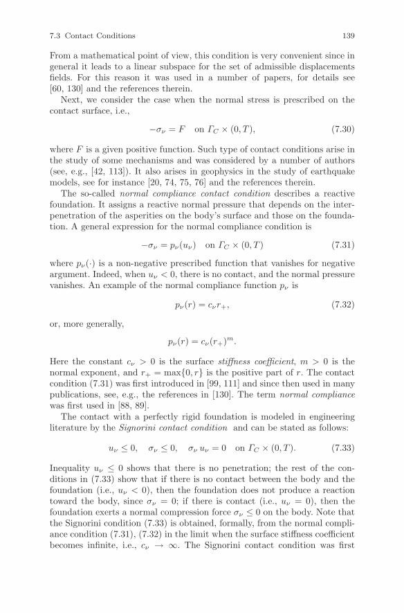
7.3 Contact Conditions 139
From a mathematical point of view, this condition is very convenient since ingeneral it leads to a linear subspace for the set of admissible displacementsfields. For this reason it was used in a number of papers, for details see[60, 130] and the references therein.
Next, we consider the case when the normal stress is prescribed on thecontact surface, i.e.,
−σν = F on ΓC × (0, T ), (7.30)
where F is a given positive function. Such type of contact conditions arise inthe study of some mechanisms and was considered by a number of authors(see, e.g., [42, 113]). It also arises in geophysics in the study of earthquakemodels, see for instance [20, 74, 75, 76] and the references therein.
The so-called normal compliance contact condition describes a reactivefoundation. It assigns a reactive normal pressure that depends on the inter-penetration of the asperities on the body’s surface and those on the founda-tion. A general expression for the normal compliance condition is
−σν = pν(uν) on ΓC × (0, T ) (7.31)
where pν(·) is a non-negative prescribed function that vanishes for negativeargument. Indeed, when uν < 0, there is no contact, and the normal pressurevanishes. An example of the normal compliance function pν is
pν(r) = cνr+, (7.32)
or, more generally,
pν(r) = cν(r+)m.
Here the constant cν > 0 is the surface stiffness coefficient, m > 0 is thenormal exponent, and r+ = max0, r is the positive part of r. The contactcondition (7.31) was first introduced in [99, 111] and since then used in manypublications, see, e.g., the references in [130]. The term normal compliancewas first used in [88, 89].
The contact with a perfectly rigid foundation is modeled in engineeringliterature by the Signorini contact condition and can be stated as follows:
uν ≤ 0, σν ≤ 0, σν uν = 0 on ΓC × (0, T ). (7.33)
Inequality uν ≤ 0 shows that there is no penetration; the rest of the con-ditions in (7.33) show that if there is no contact between the body and thefoundation (i.e., uν < 0), then the foundation does not produce a reactiontoward the body, since σν = 0; if there is contact (i.e., uν = 0), then thefoundation exerts a normal compression force σν ≤ 0 on the body. Note thatthe Signorini condition (7.33) is obtained, formally, from the normal compli-ance condition (7.31), (7.32) in the limit when the surface stiffness coefficientbecomes infinite, i.e., cν → ∞. The Signorini contact condition was first

140 7 Modeling of Contact Processes
introduced in [131] and then used in many papers, see, e.g., [130] for furtherdetails and references.
7.4 Coulomb’s Law of Dry Friction
We turn now to the conditions in the tangential directions, called also fric-tional conditions or friction laws. The simplest one is the so-called frictionlesscondition in which the friction force vanishes during the process, i.e.,
στ = 0 on ΓC × (0, T ). (7.34)
This is an idealization of the process, since even completely lubricated sur-faces generate shear resistance to tangential motion. However, (7.34) is asufficiently good approximation of the reality in some situations.
In the case when the friction force στ does not vanish on the contact sur-face, the contact is frictional. Frictional contact is usually modeled with theCoulomb law of dry friction or its variants. According to this law, the mag-nitude of the tangential traction στ is bounded by a function, the so-calledfriction bound, which is the maximal frictional resistance that the surface cangenerate; also, once slip starts, the frictional resistance opposes the directionof the motion and its magnitude reaches the friction bound. Thus,
‖στ‖ ≤ g, στ = − guτ
‖uτ‖ if uτ = 0 on ΓC × (0, T ), (7.35)
where uτ is the tangential velocity or slip rate and g represents the frictionbound. On a nonhomogeneous surface, g depends explicitly on the positionx on the surface; it also depends on the process variables, and we describethis dependence below in this section.
Note that the Coulomb law (7.35) is characterized by the existence of stick-slip zones on the contact boundary at each time moment t ∈ [0, T ]. Indeed, itfollows from (7.35) that if in a point x ∈ ΓC the inequality ‖στ (x, t)‖ < g(x)holds, then uτ (x, t) = 0 and the material point x is in the so-called stickzone; if ‖στ (x, t)‖ = g(x), then the point x is in the so-called slip zone. Weconclude that Coulomb’s friction law (7.35) models the phenomenon that slipmay occur only when the magnitude of the friction force reaches a criticalvalue, the friction bound g.
In certain applications, especially where the bodies are light or the frictionis very large, the function g in (7.35) does not depend on the process variablesand behaves like a function that depends only on the position x on the contactsurface. Considering
g = g(x), (7.36)

7.4 Coulomb’s Law of Dry Friction 141
in (7.35) leads to the Tresca friction law, and it simplifies considerably theanalysis of the corresponding contact problem, see for instance [60, 130].
Often, especially in engineering literature, the friction bound g is chosen as
g = g(σν) = µ |σν | (7.37)
where µ ≥ 0 is the coefficient of friction. The choice (7.37) in (7.35) leads tothe classical version of Coulomb’s law, which was intensively studied in theliterature, see for instance the references in [130].
When the wear of the contacting surface is taken into account, a modifiedversion of Coulomb’s law is more appropriate. This law has been derived in[139, 140, 141] from thermodynamic considerations and is given by choosing
g = µ |σν | (1 − δ|σν |)+ (7.38)
in (7.35), where δ is a very small positive parameter related to the wearconstant of the surface and, again, µ is the coefficient of friction.
The choice (7.30) in (7.37) leads to the friction bound
g = µ F (7.39)
and the choice (7.30) in (7.38) leads to the friction bound
g = µ F (1 − δF )+. (7.40)
It follows from (7.39) and (7.40) that, in the case when µ and δ are given,the friction bound g is a given function defined on the contact surface ΓC ,and therefore we recover the Tresca friction law.
We observe that the friction coefficient µ is not an intrinsic thermody-namic property of a material, a body or its surface, since it depends on thecontact process and the operating conditions. The issue is considerably com-plicated by the following facts. Engineering surfaces are not mathematicallysmooth surfaces but contain asperities and various irregularities. Moreover,very often they contain some or all of the following: moisture, lubrication oils,various debris, wear particles, oxide layers, chemicals and materials that aredifferent from those of the parent body. Therefore, it is not surprising thatthe friction coefficient is found to depend on the surface characteristics, onthe surface geometry and structure, on the relative velocity between the con-tacting surfaces, on the surface temperature, on the wear or rearrangementof the surface, and, therefore, on its history. A very thorough description ofthese issues can be found in [119] (see also the survey [142]).
Until very recently, mathematical models for frictional contact used a con-stant friction coefficient, mainly for mathematical reasons. This is rapidlychanging, and the dependence of µ on the process parameters has been incor-porated into the models in recent publications. Thus, the choice
µ = µ (‖uτ‖) (7.41)

142 7 Modeling of Contact Processes
was considered in many geophysical publications to model the motion oftectonic plates (see, e.g., [20, 119, 137] and the references therein); also, thechoice
µ = µ (‖uτ‖) (7.42)
was considered by many authors, see for instance the references in [130].Assumptions (7.41) and (7.42) allow the coefficient of friction µ to dependon the slip uτ or on the slip rate uτ , respectively.
A version of the dependence (7.41) and (7.42) may be obtained by assum-ing that the coefficient of friction depends on the total slip or on the totalslip rate of the surface, that is,
µ = µ (Su(t)) (7.43)
or
µ = µ (Su(t)), (7.44)
respectively. Here
Sw(t) =
∫ t
0
‖wτ (s)‖ ds, (7.45)
and the functions Su(x, t) and Su(x, t) represent the total slip and the totalslip rate at the point x on ΓC over the time period [0, t], respectively.
Assume again that the choice (7.30) is made in (7.37) or (7.38) and there-fore, as seen above, the friction bounds (7.39) or (7.40) are obtained. Then,taking into account the dependence (7.41) or (7.42), we obtain that the fric-tion bound g satisfies
g = g(‖uτ‖) (7.46)
or
g = g(‖uτ‖). (7.47)
The previous equalities allow the friction bound g to depend on the slip uτ
or on the slip rate uτ . For this reason, the friction law (7.35) associated to(7.46) will be called a slip-dependent friction law and the same friction law(7.35) associated to (7.47) will be called a slip rate–dependent friction law.
A similar argument based on the dependence (7.43) or (7.44) shows thatthere is a need to extend the Tresca friction law by considering the case
g = g(Su(t)) (7.48)
or
g = g(Su(t)). (7.49)
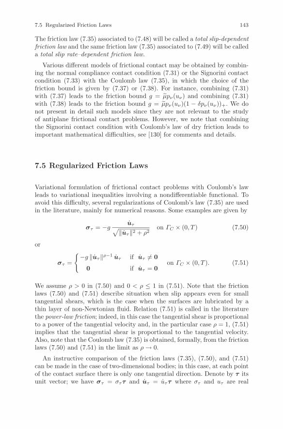
7.5 Regularized Friction Laws 143
The friction law (7.35) associated to (7.48) will be called a total slip-dependentfriction law and the same friction law (7.35) associated to (7.49) will be calleda total slip rate–dependent friction law.
Various different models of frictional contact may be obtained by combin-ing the normal compliance contact condition (7.31) or the Signorini contactcondition (7.33) with the Coulomb law (7.35), in which the choice of thefriction bound is given by (7.37) or (7.38). For instance, combining (7.31)with (7.37) leads to the friction bound g = µpν(uν) and combining (7.31)with (7.38) leads to the friction bound g = µpν(uν)(1 − δpν(uν))+. We donot present in detail such models since they are not relevant to the studyof antiplane frictional contact problems. However, we note that combiningthe Signorini contact condition with Coulomb’s law of dry friction leads toimportant mathematical difficulties, see [130] for comments and details.
7.5 Regularized Friction Laws
Variational formulation of frictional contact problems with Coulomb’s lawleads to variational inequalities involving a nondifferentiable functional. Toavoid this difficulty, several regularizations of Coulomb’s law (7.35) are usedin the literature, mainly for numerical reasons. Some examples are given by
στ = −guτ√
‖uτ‖2 + ρ2on ΓC × (0, T ) (7.50)
or
στ =
−g ‖uτ‖ρ−1 uτ if uτ = 0
0 if uτ = 0on ΓC × (0, T ). (7.51)
We assume ρ > 0 in (7.50) and 0 < ρ ≤ 1 in (7.51). Note that the frictionlaws (7.50) and (7.51) describe situation when slip appears even for smalltangential shears, which is the case when the surfaces are lubricated by athin layer of non-Newtonian fluid. Relation (7.51) is called in the literaturethe power-law friction; indeed, in this case the tangential shear is proportionalto a power of the tangential velocity and, in the particular case ρ = 1, (7.51)implies that the tangential shear is proportional to the tangential velocity.Also, note that the Coulomb law (7.35) is obtained, formally, from the frictionlaws (7.50) and (7.51) in the limit as ρ → 0.
An instructive comparison of the friction laws (7.35), (7.50), and (7.51)can be made in the case of two-dimensional bodies; in this case, at each pointof the contact surface there is only one tangential direction. Denote by τ itsunit vector; we have στ = σττ and uτ = uττ where στ and uτ are real

144 7 Modeling of Contact Processes
uτuτuτ
−στ −στ−στ
(a) (b) (c)
g
gg
g
Fig. 7.6 (a) The Tresca friction law (7.52); (b) the regularized friction law (7.53);(c) the power-law friction (7.54).
valued functions. Assume that a friction bound g ≥ 0 is given; then, in thisspecial case, (7.35) leads to the multivalued relation
−στ =
−g if uτ < 0
[−g, g] if uτ = 0
g if uτ > 0,
(7.52)
and (7.50) and (7.51) are given by
−στ = guτ√
u2τ + ρ2
, (7.53)
−στ =
g |uτ |ρ−1 uτ if uτ = 0
0 if uτ = 0,(7.54)
respectively. Relations (7.52), (7.53), and (7.54) are depicted in Figure 7.6.
Now, it is easy to see that (7.52) holds if and only if
−στ (vτ − uτ ) ≤ g|vτ | − g|uτ | ∀ vτ ∈ R,
which shows that (7.52) can be written in the subdifferential form
−στ ∈ ∂ϕ(uτ ), (7.55)
where ϕ : R → R is the function
ϕ(s) = g|s|. (7.56)
Note that this function is convex and continuous but it is not differentiableat s = 0. Also, (7.53) and (7.54) can be written in the form
−στ = ϕ′(uτ ) (7.57)

7.5 Regularized Friction Laws 145
ϕϕ
ss
ϕ
s
(a) (b) (c)
Fig. 7.7 (a) The potential ϕ(s) = g|s|; (b) the potential ϕ(s) = g√
s2 + ρ2 − ρ;(c) the potential ϕ(s) = g
ρ+1|s|ρ+1.
where ϕ′ represents the derivative of the function ϕ : R → R given by
ϕ(s) = g(√
s2 + ρ2 − ρ), in the case of (7.53). (7.58)
ϕ(s) =g
ρ + 1|s|ρ+1, in the case of (7.54). (7.59)
Clearly, in the last two cases above, the function ϕ is convex and differen-tiable; thus, it results from Proposition 1.39 that ϕ is subdifferentiable and∂ϕ(s) = ϕ′(s) for every s ∈ R; therefore (7.57) can be written in the form(7.55), too. We conclude that the friction laws (7.52)–(7.54) have a commonfeature, as the three of them can be cast in the form (7.55) with the corre-sponding choice of ϕ. The graphs of the potential functions (7.56), (7.58),and (7.59) are plotted in Figure 7.7.
Based on the arguments and comments above, in the next chapters of thisbook we consider frictional contact problems involving Coulomb’s law of dryfriction (7.35) associated to the choice of g given by (7.36), (7.46)–(7.49).On occasions, when g satisfies (7.36), we regularize (7.35) with the frictionlaws (7.50) or (7.51). Note that all these laws model evolutionary frictionalprocesses. However, sometimes we shall consider static versions of these laws,which are obtained by replacing the tangential velocity with the tangentialdisplacement. Thus, the static version of the friction law (7.35) is given by
‖στ‖ ≤ g, στ = − guτ
‖uτ‖ if uτ = 0 on ΓC . (7.60)
The static version of the regularized friction law (7.50) is given by
στ = −guτ√
‖uτ‖2 + ρ2on ΓC , (7.61)
and, finally, the static version of the power-law friction (7.51) is given by
στ =
−g ‖uτ‖ρ−1 uτ if uτ = 0
0 if uτ = 0on ΓC . (7.62)

146 7 Modeling of Contact Processes
The static friction laws are suitable for proportional loadings and can beconsidered a first approximation of the evolutionary friction laws. Consider-ing the static versions (7.60), (7.61), and (7.62) of the friction laws (7.35),(7.50), and (7.51), respectively, simplifies the mathematical analysis of thecorresponding mechanical problems.

Chapter 8
Antiplane Shear
In this chapter, we consider the mathematical modeling of a special typeof process, the antiplane shear. One can induce states of antiplane shear ina solid by loading it in a special way. We rarely actually load solids so asto cause them to deform in antiplane shear. However, we will find that thegoverning equations and boundary conditions for antiplane shear problemsare beautifully simple, and the solution will have many of the features of themore general case and may help us to solve the more complex problem, too.For this reason, in the recent years considerable attention has been paid tothe analysis of antiplane shear deformation within the context of elasticitytheory. We start the description of the basic assumptions, then we special-ize the equilibrium and constitutive equations in the context of antiplaneshear and introduce a Sobolev-type space used in the study of such kindof problems. Further, we consider an elastic antiplane displacement-tractionboundary value problem, derive its variational formulation, and prove theexistence of the unique weak solution by using the Lax-Milgram theorem.Finally, we present a complete description of the frictional contact conditionsused in this book, in the context of antiplane process; to this end, we considerboth the case of unstressed and pre-stressed reference configurations.
8.1 Basic Assumptions and Equations
We will discuss antiplane shear in the context of a three-dimensional bound-ary value problem. To this end, we refer in what follows to the physicalsetting described in Section 7.1. We assume that B is a cylinder with gener-ators parallel to the x3-axes having a cross section that is a regular regionΩ in the x1, x2-plane, Ox1x2x3 being a Cartesian coordinate system. Thecylinder is assumed to be sufficiently long so that end effects in the axialdirection are negligible. Thus, B = Ω × (−∞,+∞). Let ∂Ω = Γ ; we assumethat Γ is composed of three sets Γ 1, Γ 2, and Γ 3, with the mutually disjoint
147

148 8 Antiplane Shear
relatively open sets Γ1, Γ2, and Γ3, such that the one-dimensional measure ofΓ1, denoted meas Γ1, is strictly positive. We choose ΓD = Γ1 × (−∞,+∞),ΓF = Γ2 × (−∞,+∞), and ΓC = Γ3 × (−∞,+∞), and, according to the de-scription presented in Section 7.1, we assume that the cylinder is clamped onΓ1 ×(−∞,+∞) and is in contact with a rigid foundation on Γ3 ×(−∞,+∞).Moreover, the cylinder is subjected to time-dependent volume forces of den-sity f0 in Ω×(−∞,∞) and to time-dependent surface tractions of density f2
on Γ2 × (−∞,+∞). This physical setting is depicted in Figures 8.1 and 8.2.
Let T > 0 and let [0, T ] denote the time interval of interest. We assumethat
f0 = (0, 0, f0) with f0 = f0(x1, x2, t) : Ω × [0, T ] → R, (8.1)
f2 = (0, 0, f2) with f2 = f2(x1, x2, t) : Γ2 × [0, T ] → R. (8.2)
The body forces (8.1) and the surface tractions (8.2) give rise to a deformationof the elastic cylinder whose displacement u is of the form
u = (0, 0, u) with u = u(x1, x2, t) : Ω × [0, T ] → R. (8.3)
B
O
X
X
X2
1
3
f0
u
f2
Fig. 8.1 Antiplane shear: three-dimensional view of the cylinder.
ν
Ω
O
X
X
1
2
Γ2
Γ3
1Γ
Fig. 8.2 Antiplane shear: cross section of the cylinder in contact with a foundation.

8.1 Basic Assumptions and Equations 149
Such a deformation is called an antiplane shear. This displacement field maybe regarded as a natural complement to that of plane strain where u =(u1, u2, 0) and u1 = u1(x1, x2, t), u2 = u2(x1, x2, t), see for instance [96,p. 134] for details.
From (8.3) and (7.4) we see that, in the case of the antiplane process, theinfinitesimal strain tensor becomes
ε(u) =
0 0 12 u,1
0 0 12 u,2
12 u,1
12 u,2 0
(8.4)
and note that tr(ε(u)) = εkk(u) = 0.
Let σ = (σij) denote the stress field and recall that in the quasistaticprocesses it satisfies the equilibrium equation (7.1). Since Div σ = (σij,j), itfollows from (8.1) that
σ11,1 + σ12,2 + σ13,3 = 0
σ21,1 + σ22,2 + σ23,3 = 0
σ31,1 + σ32,2 + σ33,3 + f0 = 0
in B × (0, T ). (8.5)
Assume now that the cylinder is elastic and its behavior is modeled withthe linear isotropic constitutive law (7.23), in which µ = µ(x1, x2). We com-bine (7.23) and (8.4) to see that in this case σ = 2µε, that is,
σ =
0 0 µu,1
0 0 µu,2
µu,1 µu,2 0
. (8.6)
Since the functions u and f0 depend only on the variables x1, x2 and t andµ = µ(x1, x2), it follows from (8.6) that the first two equations in (8.5) aresatisfied identically; moreover, the last equation in (8.5) becomes
div (µ∇ u) + f0 = 0 in Ω × (0, T ). (8.7)
Here and everywhere in the rest of the book, we use the notation div and∇ for the divergence and gradient operators with respect to the variables x1
and x2, i.e.,
div τ = τ1,1 + τ2,2, (8.8)
∇v = (v,1, v,2) (8.9)
if τ = (τ1(x1, x2, t), τ2(x1, x2, t)) or τ = (τ1(x1, x2), τ2(x1, x2)) and v =v(x1, x2, t) or v = v(x1, x2). We conclude that, in the case of antiplaneshear of elastic materials, the equation of equilibrium reduces to the scalar

150 8 Antiplane Shear
equation (8.7). Note that this equation describes the nonhomogeneous casesince, here and below we assume that µ = µ(x1, x2). Antiplane shear de-formations for a nonhomogeneous anisotropic linearly elastic cylinder wereconsidered in [69, 71]. In the homogeneous case, equation (8.7) reduces to thetime-dependent Laplace equation µ ∆u + f0 = 0 in Ω × (0, T ).
Assume now that the behavior of the cylinder’s material is modeledwith a viscoelastic constitutive law with short memory, (7.24), in whichµ = µ(x1, x2) and θ = θ(x1, x2). Then, using similar arguments as above,it follows that the stress tensor is given by
σ =
0 0 θu,1 + µu,1
0 0 θu,2 + µu,2
θu,1 + µu,1 θu,2 + µu,2 0
(8.10)
and the equilibrium equation becomes
div (θ ∇u + µ∇u) + f0 = 0 in Ω × (0, T ). (8.11)
Finally, consider the case of viscoelastic materials with long memory,(7.25), in which µ = µ(x1, x2) and θ = θ(x1, x2, t); then, it follows that
σ =
0 0 σ13
0 0 σ23
σ13 σ23 0
, (8.12)
where the nonvanishing components σij at the moment t are given by
σ13(t) = σ31(t) = µu,1(t) +
∫ t
0
θ(t − s) u,1(s) ds, (8.13)
σ23(t) = σ32(t) = µu,2(t) +
∫ t
0
θ(t − s) u,2(s) ds. (8.14)
Moreover, the equation of equilibrium reduces to the scalar equation
div
(µ∇u(t) +
∫ t
0
θ(t − s)∇u(s) ds
)+ f0(t) = 0 in Ω, ∀ t ∈ [0, T ].
(8.15)
We now discuss the displacement-traction boundary conditions. Recallthat, since the cylinder is clamped on Γ1 × (−∞,+∞) × (0, T ), the dis-placement field vanishes there. Thus, (8.3) implies that
u = 0 on Γ1 × (0, T ). (8.16)

8.1 Basic Assumptions and Equations 151
Let ν denote the unit normal on Γ × (−∞,+∞),
ν = (ν1, ν2, 0) with νi = νi(x1, x2) : Γ → R, i = 1, 2. (8.17)
Denote by ∂ν u and ∂ν u the normal derivative of the displacement andvelocity, respectively, given by
∂νu = ∇ u · ν = u,1 ν1 + u,2 ν2, (8.18)
∂ν u = ∇ u · ν = u,1 ν1 + u,2 ν2. (8.19)
We use this notation to see that the Cauchy stress vector σν = (σijνj) hasthe following form:
σν = (0, 0, µ ∂νu) (8.20)
in the elastic case (8.6),
σν = (0, 0, θ ∂ν u + µ ∂νu) (8.21)
in the viscoelastic case with short memory (8.10), and
σν(t) =
(0, 0, µ ∂νu(t) +
∫ t
0
θ(t − s) ∂νu(s) ds
)(8.22)
in the viscoelastic case with long-term memory (8.12)–(8.14).
We use now (8.20)–(8.22) and (8.2) to see that the traction boundarycondition (7.3) is given by:
µ ∂νu = f2 on Γ2 × (0, T ) (8.23)
in the case of elastic materials,
θ ∂ν u + µ ∂νu = f2 on Γ2 × (0, T ) (8.24)
in the case of viscoelastic materials with short memory, and, finally,
µ ∂νu(t) +
∫ t
0
θ(t − s) ∂νu(s) ds = f2(t) on Γ2, ∀ t ∈ [0, T ] (8.25)
in the case of viscoelastic materials with long memory.
Assume now that the body forces and surface traction do not depend ontime, and the cylinder is elastic. Assume also that the displacement fieldu does not depend on time. Then the process is static and the equilibriumequation (8.7), the displacement boundary condition (8.16), and the tractionboundary condition (8.23) are valid in Ω, on Γ1, and on Γ2, respectively.
The frictional contact conditions on Γ3 will be discussed in Section 8.4;there, we specialize the contact conditions and the friction laws presented inSections 7.3–7.5 in the context of antiplane problems.

152 8 Antiplane Shear
8.2 A Function Space for Antiplane Problems
It follows from the previous section that the study of antiplane problems leadsto second-order boundary value problems in the regular domain Ω ⊂ R
2. Forthis reason, in order to impose the essential boundary condition (8.16), weintroduce the functional space V given by
V = v ∈ H1(Ω) : v = 0 on Γ1 . (8.26)
Here, equality v = 0 on Γ1 is understood in the sense of traces, i.e., almosteverywhere on Γ1, as it was described in Section 2.3. Since the trace operatoris linear and continuous, we see that V is a closed subspace of the Sobolevspace H1(Ω); therefore, combining Corollary 2.8 and Theorem 1.25, it followsthat V is a separable Hilbert space with the inner product (·, ·)H1(Ω) and theassociated norm ‖ · ‖H1(Ω).
In the study of antiplane problems, it is more convenient to consider adifferent inner product on V , defined by
(u, v)V = (∇u, ∇v)L2(Ω)2 , (8.27)
where (·, ·)L2(Ω)2 denotes the inner product on the space L2(Ω)2, (2.3). Also,denote by ‖ · ‖V the associated norm, that is,
‖v‖V = ‖∇v‖L2(Ω)2 ∀ v ∈ V. (8.28)
We have the following result.
Theorem 8.1. The space V is a separable Hilbert space with the inner prod-uct (8.27).
Proof. We apply Corollary 2.17 to see that there exists a constant c > 0,which depends on Ω and Γ1, such that
‖v‖H1(Ω) ≤ c
(‖∇v‖L2(Ω)2 +
∫
Γ1
|v| da
)∀ v ∈ H1(Ω).
Therefore, by the definition of V we obtain that
‖v‖H1(Ω) ≤ c ‖∇v‖L2(Ω)2 ∀ v ∈ V. (8.29)
Inequality (8.29) is called the Friedrichs-Poincare inequality. As a conse-quence of this inequality, it follows that (8.27) is an inner product on thespace V and, moreover,
‖v‖H1(Ω) ≤ c ‖v‖V ∀ v ∈ V. (8.30)
On the other hand, note that (8.28) and (2.10) imply that
‖v‖V ≤ ‖v‖H1(Ω) ∀ v ∈ V. (8.31)

8.2 A Function Space for Antiplane Problems 153
We combine now (8.30) and (8.31) to see that ‖ · ‖V and ‖ · ‖H1(Ω) areequivalent norms on the space V , which concludes the proof. ⊓⊔
Now, we combine (2.11) and (8.30) to see that there exists c > 0, whichdepends on Ω and Γ1, such that
‖v‖L2(Γ ) ≤ c ‖v‖V ∀ v ∈ V ; (8.32)
this implies that
‖v‖L2(Γ3) ≤ c0 ‖v‖V ∀ v ∈ V, (8.33)
where now c0 > 0 depends on Ω, Γ1, and Γ3. Inequality (8.33) will be used inseveral occasions in Part IV of the book in order to estimate various quantitiesdefined on the contact surface Γ3.
We end this section with a Green-type formula that will be repeatedlyused in the rest of the book in order to derive variational formulations ofantiplane contact problems. To this end we recall (8.8), (8.9) and we notethat, with the notation made there, the equalities below hold:
τ · ν = τ1ν1 + τ2ν2, τ · ∇ v = τ1v,1 + τ2v,2. (8.34)
We have the following result.
Theorem 8.2. Let τ = (τ 1, τ 2) ∈ H1(Ω)2. Then
∫
Ω
τ · ∇v dx +
∫
Ω
div τ v dx =
∫
Γ
τ · ν v da ∀ v ∈ H1(Ω). (8.35)
Proof. Let v ∈ H1(Ω). First, we note that
∫
Ω
w v,i dx +
∫
Ω
w,i v dx =
∫
Γ
w v νi da ∀w ∈ H1(Ω), i = 1, 2. (8.36)
This equality can be proved first for C∞(Ω) functions by an integration byparts and then extended to H1(Ω) by a density argument. We use (8.36) fori = 1 and w = τ1, then for i = 2 and w = τ2, add the resulting equalities anduse notation (8.8), (8.9), and (8.34) to obtain (8.35). ⊓⊔
Note that (8.35) implies that
∫
Ω
τ · ∇v dx +
∫
Ω
div τ v dx =
∫
Γ2
τ · ν v da +
∫
Γ3
τ · ν v da ∀ v ∈ V, (8.37)
since the boundary integral is split over Γ1, Γ2, and Γ3 and every elementv ∈ V vanishes on Γ1.

154 8 Antiplane Shear
8.3 An Elastic Antiplane Boundary Value Problem
In this section, we provide a first existence and uniqueness result in the studyof antiplane problems. We assume that the material is elastic and Γ3=∅, that is,we consider a purely displacement-traction problem. We also assume that theprocess is static and therefore the problem can be formulated as follows.
Problem 8.3. Find a displacement field u : Ω → R such that
div (µ∇u) + f0 = 0 in Ω, (8.38)
u = 0 on Γ1, (8.39)
µ ∂νu = f2 on Γ2. (8.40)
Note that (8.38), (8.39), and (8.40) represent the equilibrium equation(8.7), the displacement boundary condition (8.16), and the traction boundarycondition (8.23), respectively, in their static version. Once the displacementfield that solves Problem 8.3 is known, then the associated stress tensor σ
can be calculated by using (8.6). Also, note that in the homogeneous case(i.e., in the case when µ does not depend on x1, x2), Problem 8.3 reduces toa simple Dirichlet-Neumann problem for the Laplace equation.
Problem 8.3 is called the classical formulation of the elastic antiplanedisplacement-traction problem. In its formulation, it was assumed that allthe functions used are as smooth as is needed for the various mathematicaloperations to be justified. A function u : Ω → R is a classical solution toProblem 8.3 if u is a regular function (say u ∈ C2(Ω)∩C1(Ω)) and it satisfies(8.38) at each point x ∈ Ω, (8.39) at each point x ∈ Γ1, and (8.40) at eachpoint x ∈ Γ2.
To allow for the equations and conditions to be satisfied in a “weaker sense”we need to reformulate the problem in the so-called variational formulation,which we proceed to do. To this end we use below the space V (page 152)together with the inner product (·, ·)V and norm ‖ · ‖V and we start with thefollowing result.
Lemma 8.4. (1) Let u be a solution to Problem 8.3 such that u ∈ V andµ∇u ∈ H1(Ω)2. Then f0 ∈ L2(Ω), f2 ∈ L2(Γ2) and u satisfies the variationalequation
∫
Ω
µ∇u · ∇v dx =
∫
Ω
f0 v dx +
∫
Γ2
f2 v da ∀ v ∈ V. (8.41)
(2) Conversely, let f0 ∈ L2(Ω), f2 ∈ L2(Γ2) and consider a solution u ofthe variational equation (8.41) such that u ∈ V and µ∇u ∈ H1(Ω)2. Thenu verifies the partial differential equation (8.38) in L2(Ω) and the boundaryconditions (8.39) and (8.40) in L2(Γ1) and L2(Γ2), respectively.
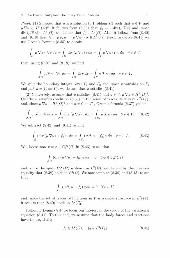
8.3 An Elastic Antiplane Boundary Value Problem 155
Proof. (1) Suppose that u is a solution to Problem 8.3 such that u ∈ V andµ∇u ∈ H1(Ω)2. It follows from (8.38) that f0 = −div (µ∇u) and, sincediv (µ∇u) ∈ L2(Ω), we deduce that f0 ∈ L2(Ω). Also, it follows from (8.40)and (8.18) that f2 = µ ∂νu = (µ∇u) · ν ∈ L2(Γ2). Next, to derive (8.41) weuse Green’s formula (8.35) to obtain
∫
Ω
µ∇u · ∇v dx +
∫
Ω
div (µ∇u) v dx =
∫
Γ
µ∇u · ν v da ∀ v ∈ V ;
then, using (8.38) and (8.18), we find
∫
Ω
µ∇u · ∇v dx =
∫
Ω
f0 v dx +
∫
Γ
µ ∂νu v da ∀ v ∈ V.
We split the boundary integral over Γ1 and Γ2 and, since v vanishes on Γ1
and µ ∂ν u = f2 on Γ2, we deduce that u satisfies (8.41).
(2) Conversely, assume that u satisfies (8.41) and u ∈ V, µ∇u ∈ H1(Ω)2.Clearly, u satisfies condition (8.39) in the sense of traces, that is in L2(Γ1),and, since µ∇u ∈ H1(Ω)2 and u = 0 on Γ1, Green’s formula (8.37) yields:
∫
Ω
µ∇u · ∇v dx +
∫
Ω
div (µ∇u) v dx =
∫
Γ2
µ ∂νu v da ∀ v ∈ V. (8.42)
We subtract (8.42) and (8.41) to find
∫
Ω
(div (µ∇u) + f0) v dx =
∫
Γ2
(µ ∂νu − f2) v da ∀ v ∈ V. (8.43)
We choose now v = ϕ ∈ C∞0 (Ω) in (8.43) to see that
∫
Ω
(div (µ∇u) + f0) ϕ dx = 0 ∀ϕ ∈ C∞0 (Ω)
and, since the space C∞0 (Ω) is dense in L2(Ω), we deduce by the previous
equality that (8.38) holds in L2(Ω). We now combine (8.38) and (8.43) to seethat
∫
Γ2
(µ ∂ν u − f2) v da = 0 ∀ v ∈ V
and, since the set of traces of functions in V is a dense subspace in L2(Γ2),it results that (8.40) holds in L2(Γ2). ⊓⊔
Following Lemma 8.4, we focus our interest in the study of the variationalequation (8.41). To this end, we assume that the body forces and tractionshave the regularity
f0 ∈ L2(Ω), f2 ∈ L2(Γ2) (8.44)

156 8 Antiplane Shear
and the Lame coefficient satisfies
µ ∈ L∞(Ω) and there exists µ∗ > 0 such that (8.45)
µ(x) ≥ µ∗ a.e. x ∈ Ω.
We denote by a : V × V → R the bilinear form
a(u, v) =
∫
Ω
µ∇u · ∇v dx (8.46)
and we note that assumption (8.45) implies that the integral in (8.46) iswell defined. We also note that by assumption (8.44), the integrals on theright-hand side of (8.41) are well defined and, moreover, the functional
v →∫
Ω
f0 v dx +
∫
Γ2
f2 v da
is a linear continuous functional on V. We use now Riesz’s representationtheorem (page 11) to define an element f ∈ V by the equality
(f, v)V =
∫
Ω
f0 v dx +
∫
Γ2
f2 v da. (8.47)
Note that (8.47) and (8.32) imply that
‖f‖V ≤ c(‖f0‖L2(Ω) + ‖f2‖L2(Γ2)
)(8.48)
where c depends on Ω and Γ1. Next, equalities (8.46), (8.47) combined withLemma 8.4 lead us to the following formulation of Problem 8.3.
Problem 8.5. Find a displacement field u ∈ V such that
a(u, v) = (f, v)V ∀ v ∈ V. (8.49)
It follows from the discussion in Lemma 8.4 that every smooth solutionof Problem 8.3 is a solution to Problem 8.5 and conversely, if Problem 8.5has a sufficiently smooth solution, it is also a solution of the original problemin the usual sense. However, now we have a formulation, the so-called vari-ational formulation, that may have solutions that do not have the necessaryregularity or smoothness, and we still call them solutions, but now we writethat such solutions are weak solutions of the original problem.
The statement of the existence and uniqueness of the solution for Prob-lem 8.5 is as follows.
Theorem 8.6. Assume that (8.44) and (8.45) hold. Then Problem 8.5 has aunique solution u ∈ V. Moreover, there exists c > 0, which depends only onΩ, Γ1, and µ∗ such that
‖u‖V ≤ c (‖f0‖L2(Ω) + ‖f2‖L2(Γ2)), (8.50)

8.4 Frictional Contact Conditions 157
and the solution minimizes on V the energy functional J defined by
J(v) =1
2
∫
Ω
µ ‖∇v‖2 dx −∫
Ω
f0 v dx −∫
Γ2
f2 v dx.
Proof. The bilinear form a defined by (8.46) is symmetric and, moreover, by(8.45) it follows that
|a(u, v)| ≤ ‖µ‖L∞(Ω) ‖u‖V ‖v‖V ∀u, v ∈ V, (8.51)
i.e., a is continuous. It also follows (8.45) that
a(v, v) ≥ µ∗ ‖v‖2V ∀ v ∈ V, (8.52)
i.e., a is V -elliptic. The existence and uniqueness part in Theorem 8.6 is nowa consequence of the Lax-Milgram theorem (Corollary 3.5, page 47). Also,we choose v = u in (8.49) and use (8.52) to obtain
‖u‖V ≤ 1
µ∗ ‖f‖V . (8.53)
We use (8.53) and (8.48) to obtain (8.50) with a positive constant c, whichdepends only on Ω, Γ1, and µ∗. The last part of the theorem follows from(8.46) and (8.47), combined with the arguments presented on page 47. ⊓⊔
We conclude by Theorem 8.6 that the mechanical problem 8.3 has a uniqueweak solution that depends continuously on the data.
The arguments in this section will be used in the study of the antiplanefrictional contact problems presented in Part IV of the manuscript. The pat-tern is very similar for each problem: first, the classical formulation of themodel is described, which amounts to choosing the constitutive law and thecontact conditions. Then, a variational formulation of the problem is derivedby performing, formally, integration by parts and using the equations and theconditions. Next, a statement of the existence and uniqueness results, underappropriate assumptions on the problem data, is provided.
8.4 Frictional Contact Conditions
In this section, we specialize the frictional contact conditions presented inSections 7.3–7.5 to the case of antiplane shear. We first recall that for adisplacement field u, we denote by uν and uτ its normal and tangentialcomponents given by
uν = u · ν, uτ = u − uν ν.
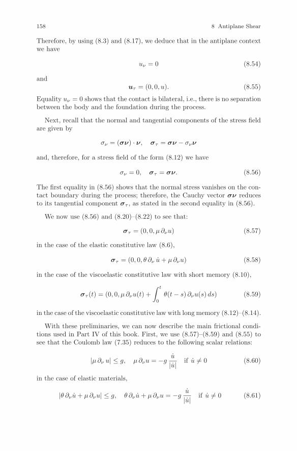
158 8 Antiplane Shear
Therefore, by using (8.3) and (8.17), we deduce that in the antiplane contextwe have
uν = 0 (8.54)
anduτ = (0, 0, u). (8.55)
Equality uν = 0 shows that the contact is bilateral, i.e., there is no separationbetween the body and the foundation during the process.
Next, recall that the normal and tangential components of the stress fieldare given by
σν = (σν) · ν, στ = σν − σνν
and, therefore, for a stress field of the form (8.12) we have
σν = 0, στ = σν. (8.56)
The first equality in (8.56) shows that the normal stress vanishes on the con-tact boundary during the process; therefore, the Cauchy vector σν reducesto its tangential component στ , as stated in the second equality in (8.56).
We now use (8.56) and (8.20)–(8.22) to see that:
στ = (0, 0, µ ∂νu) (8.57)
in the case of the elastic constitutive law (8.6),
στ = (0, 0, θ ∂ν u + µ ∂νu) (8.58)
in the case of the viscoelastic constitutive law with short memory (8.10),
στ (t) = (0, 0, µ ∂νu(t) +
∫ t
0
θ(t − s) ∂νu(s) ds) (8.59)
in the case of the viscoelastic constitutive law with long memory (8.12)–(8.14).
With these preliminaries, we can now describe the main frictional condi-tions used in Part IV of this book. First, we use (8.57)–(8.59) and (8.55) tosee that the Coulomb law (7.35) reduces to the following scalar relations:
|µ ∂ν u| ≤ g, µ ∂νu = −gu
|u| if u = 0 (8.60)
in the case of elastic materials,
|θ ∂ν u + µ ∂νu| ≤ g, θ ∂ν u + µ ∂νu = −gu
|u| if u = 0 (8.61)
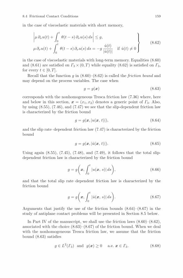
8.4 Frictional Contact Conditions 159
in the case of viscoelastic materials with short memory,
∣∣∣∣µ ∂νu(t) +
∫ t
0
θ(t − s) ∂νu(s) ds
∣∣∣∣ ≤ g,
µ ∂νu(t) +
∫ t
0
θ(t − s) ∂νu(s) ds = −gu(t)
|u(t)| if u(t) = 0
(8.62)
in the case of viscoelastic materials with long-term memory. Equalities (8.60)and (8.61) are satisfied on Γ3 × (0, T ) while equality (8.62) is satisfied on Γ3,for every t ∈ [0, T ].
Recall that the function g in (8.60)–(8.62) is called the friction bound andmay depend on the process variables. The case when
g = g(x) (8.63)
corresponds with the nonhomogeneous Tresca friction law (7.36) where, hereand below in this section, x = (x1, x2) denotes a generic point of Γ3. Also,by using (8.55), (7.46), and (7.47) we see that the slip-dependent friction lawis characterized by the friction bound
g = g(x, |u(x, t)|), (8.64)
and the slip rate–dependent friction law (7.47) is characterized by the frictionbound
g = g(x, |u(x, t)|). (8.65)
Using again (8.55), (7.45), (7.48), and (7.49), it follows that the total slip-dependent friction law is characterized by the friction bound
g = g
(x,
∫ t
0
|u(x, s)| ds
), (8.66)
and that the total slip rate–dependent friction law is characterized by thefriction bound
g = g
(x,
∫ t
0
|u(x, s)| ds
). (8.67)
Arguments that justify the use of the friction bounds (8.64)–(8.67) in thestudy of antiplane contact problems will be presented in Section 8.5 below.
In Part IV of the manuscript, we shall use the friction laws (8.60)–(8.62),associated with the choice (8.63)–(8.67) of the friction bound. When we dealwith the nonhomogeneous Tresca friction law, we assume that the frictionbound (8.63) satisfies
g ∈ L2(Γ3) and g(x) ≥ 0 a.e. x ∈ Γ3. (8.68)

160 8 Antiplane Shear
Also, when we use the friction bounds (8.64)–(8.67), we assume that
(a) g : Γ3 × R → R+.
(b) There exists Lg > 0 such that|g(x, r1) − g(x, r2)| ≤ Lg |r1 − r2|
∀ r1, r2 ∈ R, a.e. x ∈ Γ3.
(c) The mapping x → g(x, r)is Lebesgue measurable on Γ3, ∀ r ∈ R.
(d) The mapping x → g(x, 0) belongs to L2(Γ3).
(8.69)
Note that condition (8.69)(b) requires that g(x, ·) : R → R+ is a Lipschitzcontinuous function, uniformly with respect to x ∈ Γ3; the rest of the condi-tions in (8.69) are introduced for mathematical reasons, since they guaranteethat the mapping x → g(x, ζ(x)) belongs to L2(Γ3) whenever ζ ∈ L2(Γ3).
Next, we use again equalities (8.57)–(8.59) and (8.55) to see that, in theantiplane shear context, the regularized friction law (7.50) reduces to thefollowing scalar relations:
µ ∂νu = −gu√
u2 + ρ2(8.70)
in the case of elastic materials,
θ ∂ν u + µ ∂ν u = −gu√
u2 + ρ2(8.71)
in the case of viscoelastic materials with short memory,
µ ∂νu(t) +
∫ t
0
θ(t − s) ∂νu(s) ds = −gu(t)√
u(t)2 + ρ2(8.72)
in the case of viscoelastic materials with long memory. Here ρ > 0 is aregularization parameter.
Also, the power-law friction (7.51) reduces to the following scalar relations:
µ ∂νu =
−g |u|ρ−1 u if u = 0
0 if u = 0(8.73)
in the case of elastic materials,
θ ∂ν u + µ ∂νu =
−g |u|ρ−1 u if u = 0
0 if u = 0(8.74)
in the case of viscoelastic materials with short memory,
µ ∂νu(t) +
∫ t
0
θ(t − s) ∂νu(s) ds =
−g |u|ρ−1 u if u = 0
0 if u = 0(8.75)

8.4 Frictional Contact Conditions 161
in the case of viscoelastic materials with long memory. Here, ρ is a regular-ization parameter and is assumed to satisfy 0 < ρ ≤ 1.
Equalities (8.70), (8.71), (8.73), and (8.74) are satisfied on Γ3 × (0, T ) andequalities (8.72) and (8.75) are satisfied on Γ3, for every t ∈ [0, T ]. In thisbook, we provide results in the study of antiplane contact problems involvingfriction laws of the form (8.70)–(8.72) under the assumption (8.68) on g. Partof these results can be extended to antiplane contact problems involvingfriction laws of the form (8.73)–(8.75). However, to avoid repetitions, werestrict ourselves to the case of elastic materials and, therefore, we use thefriction law (8.73); we assume in this case that g ∈ L∞(Γ3) is a positivefunction.
The friction laws (8.60)–(8.62) model a situation in which surfaces aredry; they are characterized by the existence of a positive function, the fric-tion bound, such that slip may occur only when the friction force reaches thecritical value provided by the friction bound. The friction laws (8.70)–(8.75)do not have this feature, since in their case slip appears even for small tan-gential shear. Such kind of situations appear in practice when the contactsurfaces are lubricated.
We note that the friction conditions above are formulated in the evolu-tionary case. The static case is obtained by replacing the velocity u with thedisplacement u in the corresponding formulas. To provide some examples, wesee that the static version of (8.60) is given by
|µ ∂νu| ≤ g, µ ∂νu = −gu
|u| if u = 0, (8.76)
the static version of (8.70) is given by
µ ∂ν u = −gu√
u2 + ρ2, (8.77)
and the static version of (8.73) is given by
µ ∂νu =
−g |u|ρ−1 u if u = 0
0 if u = 0.(8.78)
Equalities (8.76)–(8.78) are satisfied on Γ3. Note also that the static versionof the friction laws should be seen either as a model suitable for proportionalloadings or as a first approximation of the evolutionary ones.
We end this section with the remark that in the physical setting of theantiplane problems described above, the normal component of the stress van-ishes on the contact surface during the process, see (8.56). This feature is notincompatible with the choice (7.36) for the friction bound, which correspondswith the Tresca friction law. However, we note that the use of the choice (7.37)or (7.38) leads to the friction bound g = 0 and, therefore, the Coulomb law

162 8 Antiplane Shear
of dry friction (7.35) implies that the friction force vanishes on the contactsurface, i.e., the contact is frictionless. We conclude that the choice (7.37) or(7.38) for the friction bound is not appropriate with the study of antiplanefrictional problems in the physical setting above.
For this reason, in order to accommodate the classical and the modifiedCoulomb law of dry friction with the antiplane context, in the next sectionwe present models for frictional contact that involve antiplane shear defor-mations in a slightly different physical setting. In these models, the normalstress on the contact surface does not vanish and, therefore, the use of theCoulomb law of dry friction with the choice (7.37) or (7.38) makes sense, asit is compatible with a genuine frictional condition.
8.5 Antiplane Models for Pre-stressed Cylinders
The models of antiplane shear deformation studied in the previous sectionsof this chapter were derived under the assumption that the reference configu-ration of the cylindrical body is unstressed, i.e., in absence of body forces andtractions, the stress tensor vanishes. However, there is a need to consider thecase when the body is in a pre-stressed reference configuration, i.e., besidesthe external loads that give rise to stresses and deformations, the body is sub-mitted to pre-loads that induce a primary stress. This stress, denoted in whatfollows σP , plays the role of a “self-equilibrating stress,” since it is in equi-librium with the pre-loads that keep the body in the reference configuration.Concrete situations of such type arise in the geophysical models that describethe systems of faults in a domain (see, e.g., [20, 74, 81]) as well as in the studyof pre-stressed composite assemblies (see, e.g., [97, 118, 127]). They also arisein the study of mining engineering problems (see, e.g., [34, 35]), where the ref-erence configuration of the rocks is supposed to be stressed before excavation.
In this section, we provide models for the antiplane frictional contact prob-lems in the case when the cylindrical body B is in a pre-stressed referenceconfiguration. To this end, we consider again the physical setting presentedin Section 8.1 and conserve the notation introduced there; however, we ass-ume now that there exists a primary stress σP in the reference configuration,obtained by applying pre-loads and, moreover,
σP =
−F 0 0
0 −F 0
0 0 0
, (8.79)
where F is a positive constant. This last assumption is made only for the sakeof simplicity, since by using the same arguments, the results below can beextended to the case when the primary stress has a more general form. Note

8.5 Antiplane Models for Pre-stressed Cylinders 163
also that the choice (8.79) of the primary stress is inspired by the geophysicalcontext of modeling of earthquakes’ evolution, where F is interpreted as thenormal stress on the faults, see [19, 74, 76, 81] and the references therein.
It follows from assumption (8.79) that
Div σP = 0 (8.80)
and, using (7.28), (8.17), we obtain
σP ν = −Fν, σPν = −F, σP
τ = 0. (8.81)
Equality (8.80) shows that the pre-loaded body force vanishes and (8.81)implies that the pre-loaded pressure on the cylinder’s surface is −Fν.
Assume now the antiplane context (8.1)–(8.3) and denote by σ = (σij)the stress in the body associated to the deformation field (8.4), by usingone of the constitutive laws (7.23), (7.24), or (7.25); then, by the argumentspresented in Section 8.1, it follows that σ is of the form (8.12), where thecomponents σ13 and σ23 depend only on x1, x2 and t; also, the argumentspresented in Section 8.4 show that
σν = (0, 0, q), σν = 0, στ = (0, 0, q) (8.82)
where q = σ13ν1 + σ23ν2. Next, the total stress in the body after applyingthe body forces and tractions, denoted σ, is given by
σ = σ + σP . (8.83)
Therefore, combining (8.80)–(8.83) we find that
Div σ = Div σ, (8.84)
σν = σν − Fν, σν = −F, στ = στ . (8.85)
Since the pre-loaded body forces vanish, the equilibrium equation isgiven by
Div σ + f0 = 0 in B × (0, T )
and, using (8.84), we find that
Div σ + f0 = 0 in B × (0, T ).
We now use assumption (8.1) in the previous equality to recover equation(8.5). Then, we use the arguments in Section 8.1 to see that the equation ofequilibrium is given by (8.7) in the elastic case (8.6), by (8.11) in the viscoelas-tic case with short memory (8.10), and by (8.15) in the case of viscoelasticmaterials with long memory (8.13), (8.14).

164 8 Antiplane Shear
We now discuss the displacement-traction boundary conditions. Recallthat since the cylinder is fixed on ΓD × (0, T ), the displacement field vanishesthere and, therefore, by (7.2) and (8.3), we impose the displacement condition(8.16). Next, the traction boundary condition is
σν = f2 − Fν on ΓF × (0, T ),
and here we take into account the pre-loaded pressure −Fν that is actingon the boundary ΓF of the cylinder. Combining this last boundary conditionwith (8.85) we obtain
σν = f2 on ΓF × (0, T ).
Then, by the arguments presented in Section 8.1, it follows that the tractionboundary condition is given by (8.23) in the case of elastic materials, by(8.24) in the case of viscoelastic materials with short memory, and by (8.25)in the case of viscoelastic materials with long memory.
We now investigate the frictional contact conditions on ΓC × (0, T ). First,note that by (8.85) it follows that
σν = −F on ΓC × (0, T ), (8.86)
i.e., the normal stress is prescribed and does not vanish on the contact bound-ary during the process. This is the main difference with the case of unstressedconfiguration presented in Sections 8.1 and 8.4, as there the normal stressvanishes, see (8.56).
Assume now that the tangential part of the total stress σ satisfies onΓC × (0, T ) the Coulomb law of dry friction in its quasistatic form (7.35);since (8.85) implies that στ = στ , it follows that the friction force στ satisfiesthe same friction law on ΓC × (0, T ). Therefore, arguing as in Section 8.4,we obtain that the friction conditions are formulated on Γ3 × (0, T ) andare given by (8.60) in the case of elastic materials, by (8.61) in the caseof viscoelastic materials with short memory, and by (8.62) in the case ofviscoelastic materials with long memory. Note also that now σν = 0 andtherefore it follows from the discussion on page 161 that, besides the Trescafriction law corresponding with the friction bound (7.36), it make sense toconsider the classical Coulomb law of friction corresponding with the frictionbound (7.37) as well as the modified Coulomb law of friction correspondingwith the friction bound (7.38). Thus, as explained in Section 7.4, it makessense to consider slip, slip rate, total slip, and total slip rate dependent frictionlaws, which in the antiplane context lead to friction bounds of the form(8.64)–(8.67).
Similar results can be obtained by considering the static version of theantiplane frictional processes. For instance, considering the static Coulomblaw of dry friction, (7.60), we obtain that, in the case of elastic materials, thefrictional contact conditions are given by (8.76).

8.5 Antiplane Models for Pre-stressed Cylinders 165
From the discussion above, we conclude that considering antiplane fric-tional contact processes in the context of pre-stressed reference configurationsin which the primary stress σP is of the form (8.79) leads to the equation ofequilibrium and to the displacement-traction boundary conditions describedin Section 8.1, as well as to the frictional conditions described in Section 8.4.The consequence of this conclusion is twofold. First, it shows that from themathematical point of view, there is no difference between the study of an-tiplane frictional contact problems in unstressed reference configurations andthe study of antiplane frictional contact problems in pre-stressed referenceconfigurations, since these problems lead to the same mathematical models,even if their physical settings are different. Second, it justifies the use ofthe Coulomb law of dry friction with the friction bounds (8.64)–(8.67), sinceconsidering such friction bounds makes sense in the case of antiplane contactproblems formulated on pre-stressed reference configurations.
For all these reasons, in Part IV of this book we use the equations andboundary conditions in Sections 8.1 and 8.4, without specifying if the refer-ence configuration is unstressed or pre-stressed; we combine them to derivemathematical models in the study of antiplane frictional contact problemswith elastic or viscoelastic materials; then, we provide the variational analy-sis of the models by using the abstract results presented in Part II of the book.

Bibliographical Notes
For a comprehensive treatment of basic aspects of solid mechanics, the readeris referred to [6, 40, 51, 56, 84, 94, 96, 109, 110, 143] and to [26] for anin-depth mathematical treatment of three-dimensional elasticity. More infor-mation concerning the elastic and viscoelastic constitutive laws presented inSection 7.2 can be found in [41, 116, 144]. One is referred to [82, 119] formore details on the modeling aspects of contact mechanics treated in therest of Chapter 7. Experimental background and elements of surface physicsthat justify some of the contact and frictional boundary conditions presentedin Sections 7.3 and 7.4 can be found in [55, 86, 104, 111, 112, 119, 146]. Inparticular, the relationship between the Coulomb and Tresca friction law isdiscussed in [119, 146] and, there, a natural transition from the Coulomb tothe Tresca friction laws is justified. The regularization (7.50) of the Coulombfriction law was used in [75, 76] in the study of a dynamic contact problemwith slip-dependent coefficient of friction involving viscoelastic and elasticmaterials, respectively. Its static version, (7.61), was used in [65]; there, thefinite element uniqueness of a problem in linear elasticity with unilateralcontact is investigated.
Contact problems in elasticity have been studied by many authors. Thefamous Signorini problem was formulated in [131] to model the unilateralcontact between an elastic material and a rigid foundation. Mathemati-cal analysis of the Signorini problem was provided in [47] and its numer-ical analysis was performed in [86]. References concerning the Signorinicontact problem for elastic and inelastic materials include [142]. Refer-ences treating modeling and analysis of various contact problems include[42, 43, 60, 80, 86, 113, 130, 149]. Many computational methods for problemsin contact mechanics can be found in the monographs [93, 147] and in theextensive lists of references therein. The state of the art in the field can befound in the proceedings [98, 120, 148] and in the special issue [128], as well.
The model of antiplane shear deformation described in Chapter 8 of thebook represents one of the simplest classes of deformations that a solid can
167

168 Bibliographical Notes
undergo. For this reason, it was considered by many authors, and we mentionbelow some of the references on this topic.
Following the pioneering works [48, 90, 91] that led to a modern revivalof interest in antiplane shear deformations in hyperelasticity, several papershave been devoted to these deformations, see for instance [71, 72]. The pur-pose of [71] is to study the antiplane shear deformations of a nonhomogeneousanisotropic cylinder submitted to prescribed surface tractions on its lateralboundary; it is shown that, in the absence of body forces, not all arbitraryanisotropic cylinders will sustain an antiplane shear deformation; moreover,necessary and sufficient conditions on the elastic moduli are obtained that doallow an antiplane shear. The aim of [72] is to investigate the basic issues thatarise when generalized plain strain deformations are superimposed on anti-plane shear deformations in isotropic incompressible hyperelastic materials.
An excellent reference concerning antiplane shear deformations in solidmechanics is the review article [69], where modern developments for the anti-plane shear model and its applications are described for both linear andnonlinear solid materials; various physical settings (including dynamic effects)where the antiplane shear model shows promise for further development areoutlined; and some open questions concerning a challenging antiplane shearinverse problem in linear isotropic elastostatics are described.
Reference on antiplane problems in the finite strain framework include[21, 45, 62, 63, 145]. Thus, the equations governing antiplane shear mo-tions for nonlinear elastic Mooney-Rivlin materials were first derived in [21]and extended in [63] to the case of viscoelastic Mooney-Rivlin materials. In[62], some exact dynamical solutions for antiplane problems involving neo-Hookean materials are determined. The equations for antiplane shear motionsmay be found in [145], in the general case of an anisotropic nonlinear elasticmaterials, and in [45], in the framework of the nonlinear theory of viscoelasticmaterials of differential type.
An antiplane problem for incompressible isotropic viscoplastic solids wasconsidered in [54]; there, the authors use a flow rule that is a properly invari-ant generalization of Coulomb’s sliding friction law and provide a uniquenessresult in the study of the corresponding antiplane initial boundary valueproblem.
The model of antiplane shear was used in fracture mechanics to model thesituation when the crack surfaces move relatively to one another and parallelto the leading edge of the crack, see for instance [64, p. 321] for details.Following [70], the damage and local crack tip process zone are modeled infracture mechanics by using elastic antiplane problems in which the elasticcoefficients vary continuous with position. References on this topic include[23, 114], where the cracks in viscoelastic materials are studied under theantiplane shear condition.

Chapter 9
Elastic Problems
In this chapter, we study antiplane frictional contact models for elasticmaterials, both in the static and quasistatic case. We start by consideringstatic problems in which friction is described with the Tresca law and itsregularizations; we derive a variational formulation for each model that isin the form of an elliptic variational inequality for the displacement field;then we prove existence, uniqueness, and convergence results for the weaksolution. Next, we consider a static slip dependent frictional contact prob-lem that leads to an elliptic quasivariational inequality and, again, we provethe existence and uniqueness of the weak solution. We then extend part ofthe above results in the study of quasistatic versions of these models, whichlead to evolutionary variational or quasivariational inequalities. Everywherein this chapter, we use the space V (page 152) together with its inner prod-uct (·, ·)V and the associated norm ‖ · ‖V , and we denote by [0, T ] the timeinterval of interest, T > 0. Also, everywhere in this chapter, the use of theabstract results presented in Part II of this manuscript is made in the caseX = V , (·, ·)X = (·, ·)V , without explicit specification.
9.1 Static Frictional Problems
In this section, we consider static frictional antiplane problems. For the firstproblem, the friction is modeled with Tresca’s law and therefore the classicalmodel of the process is the following.
Problem 9.1. Find a displacement field u : Ω → R such that
div (µ∇u) + f0 = 0 in Ω, (9.1)u = 0 on Γ1, (9.2)
µ ∂νu = f2 on Γ2, (9.3)
|µ ∂νu| ≤ g, µ ∂νu = −gu
|u| if u = 0 on Γ3. (9.4)
171
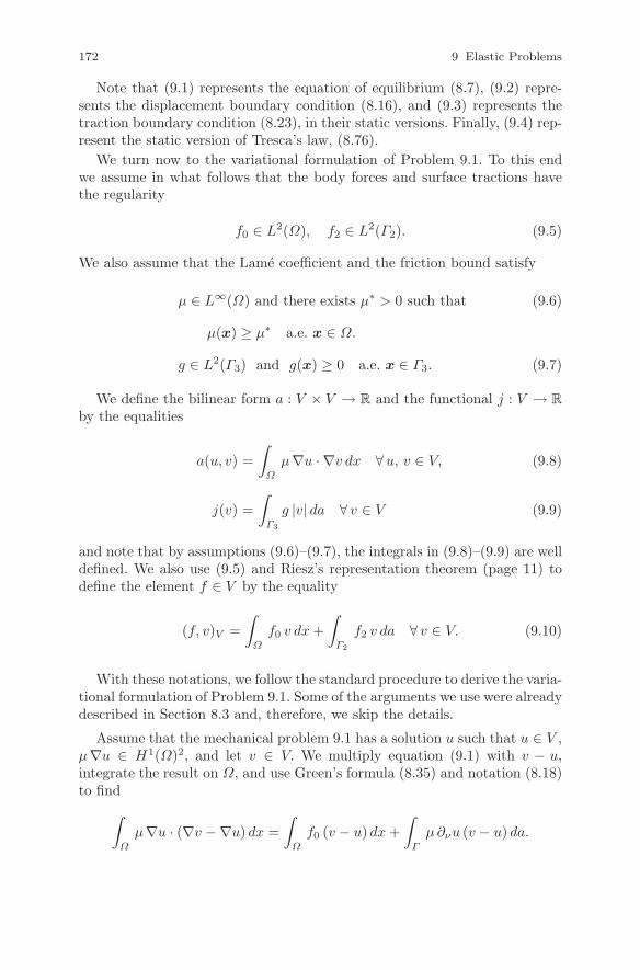
172 9 Elastic Problems
Note that (9.1) represents the equation of equilibrium (8.7), (9.2) repre-sents the displacement boundary condition (8.16), and (9.3) represents thetraction boundary condition (8.23), in their static versions. Finally, (9.4) rep-resent the static version of Tresca’s law, (8.76).
We turn now to the variational formulation of Problem 9.1. To this endwe assume in what follows that the body forces and surface tractions havethe regularity
f0 ∈ L2(Ω), f2 ∈ L2(Γ2). (9.5)
We also assume that the Lame coefficient and the friction bound satisfy
µ ∈ L∞(Ω) and there exists µ∗ > 0 such that (9.6)
µ(x) ≥ µ∗ a.e. x ∈ Ω.
g ∈ L2(Γ3) and g(x) ≥ 0 a.e. x ∈ Γ3. (9.7)
We define the bilinear form a : V × V → R and the functional j : V → R
by the equalities
a(u, v) =
∫
Ω
µ∇u · ∇v dx ∀u, v ∈ V, (9.8)
j(v) =
∫
Γ3
g |v| da ∀ v ∈ V (9.9)
and note that by assumptions (9.6)–(9.7), the integrals in (9.8)–(9.9) are welldefined. We also use (9.5) and Riesz’s representation theorem (page 11) todefine the element f ∈ V by the equality
(f, v)V =
∫
Ω
f0 v dx +
∫
Γ2
f2 v da ∀ v ∈ V. (9.10)
With these notations, we follow the standard procedure to derive the varia-tional formulation of Problem 9.1. Some of the arguments we use were alreadydescribed in Section 8.3 and, therefore, we skip the details.
Assume that the mechanical problem 9.1 has a solution u such that u ∈ V ,µ∇u ∈ H1(Ω)2, and let v ∈ V. We multiply equation (9.1) with v − u,integrate the result on Ω, and use Green’s formula (8.35) and notation (8.18)to find
∫
Ω
µ∇u · (∇v − ∇u) dx =
∫
Ω
f0 (v − u) dx +
∫
Γ
µ ∂νu (v − u) da.

9.1 Static Frictional Problems 173
We split the boundary integral over Γ1, Γ2, and Γ3 and, since v − u vanisheson Γ1 and µ ∂νu = f2 on Γ2, we deduce that
∫
Ω
µ∇u · (∇v − ∇u) dx
=
∫
Ω
f0 (v − u) dx +
∫
Γ2
f2 (v − u) da +
∫
Γ3
µ ∂νu (v − u) da. (9.11)
Now we use (9.4) to see that
µ ∂νu (v − u) ≥ g |u| − g |v| a.e. on Γ3. (9.12)
Indeed, in the points of Γ3 where u = 0 we have
µ ∂νu (v − u) = −gu
|u| (v − u) = g|u| − guv
|u| ≥ g|u| − g|v|,
as uv|u| ≤ |v|; in the points of Γ3 where u = 0 we have
µ ∂νu (v − u) = µ (∂νu) v ≥ −|µ ∂νu| |v| ≥ −g|v| = g |u| − g |v|,
as |µ ∂νu| ≤ g.
We integrate (9.12) on Γ3 to obtain
∫
Γ3
µ ∂νu (v − u) da ≥∫
Γ3
g |u| da −∫
Γ3
g |v| da
and combine this inequality with (9.11) to find
∫
Ω
µ∇u · (∇v − ∇u) dx +
∫
Γ3
g |v| da −∫
Γ3
g |u| da
≥∫
Ω
f0 (v − u) dx +
∫
Γ2
f2 (v − u) da. (9.13)
We use now the notation (9.8)–(9.10) and inequality (9.13) to derive thefollowing variational formulation of the antiplane frictional contact prob-lem 9.1.
Problem 9.2. Find a displacement field u ∈ V such that
a(u, v − u) + j(v) − j(u) ≥ (f, v − u)V ∀ v ∈ V. (9.14)
In the study of Problem 9.2 we have the following existence, uniqueness,and continuous dependence result.
Theorem 9.3. Assume that (9.5)–(9.7) hold. Then Problem 9.2 has a uniquesolution u ∈ V. Moreover, the mapping f → u:V → V is Lipschitz continuous.

174 9 Elastic Problems
Proof. The bilinear form a defined by (9.8) is symmetric, and using (8.51)and (8.52) it follows that it is continuous and V -elliptic. We use (9.7) to seethat the functional j defined by (9.9) is a seminorm on V and it satisfies
j(v) ≤ ‖g‖L2(Γ3)‖v‖L2(Γ3) ∀ v ∈ V.
Therefore, (8.33) yields
j(v) ≤ c0 ‖g‖L2(Γ3) ‖v‖V ∀ v ∈ V. (9.15)
It follows from (9.15) that the seminorm j is continuous, which implies thatit is a convex lower semicontinuous function on V . Theorem 9.3 is now aconsequence of Theorem 3.1. ⊓⊔
We conclude by Theorem 9.3 that the mechanical problem 9.1 has a uniqueweak solution that depends Lipschitz continuously on the data. Moreover, asit follows from the proof of Theorem 3.1, the solution minimizes on V theenergy functional J defined by
J(v) =1
2
∫
Ω
µ ‖∇v‖2 dx +
∫
Γ3
g |v| da −∫
Ω
f0 v dx −∫
Γ2
f2 v da.
We now study the problem in the case when the Tresca friction law (9.4)is replaced by its regularized versions. We start by considering the followingproblem.
Problem 9.4. Find a displacement field uρ : Ω → R such that
div (µ∇uρ) + f0 = 0 in Ω, (9.16)
uρ = 0 on Γ1, (9.17)
µ ∂νuρ = f2 on Γ2, (9.18)
µ ∂νuρ = −guρ√
u2ρ + ρ2
on Γ3. (9.19)
The equation and boundary conditions involved in Problem 9.4 have thesame meaning as those in Problem 9.1. The difference arises from the factthat here we replace the static version of Tresca law (9.4) with its regular-ization (9.19), introduced in (8.77), page 161. Recall that here ρ > 0 is aregularization parameter.
The variational formulation of the antiplane frictional contact problem 9.4is derived by using arguments similar to those used to derive the variationalformulation of Problem 9.1. It is obtained in several steps that are describedbelow.
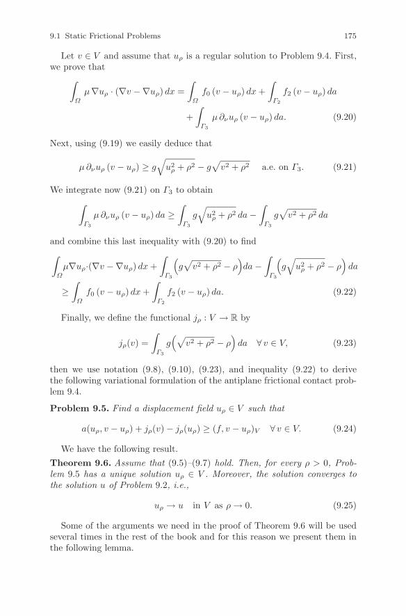
9.1 Static Frictional Problems 175
Let v ∈ V and assume that uρ is a regular solution to Problem 9.4. First,we prove that
∫
Ω
µ∇uρ · (∇v − ∇uρ) dx =
∫
Ω
f0 (v − uρ) dx +
∫
Γ2
f2 (v − uρ) da
+
∫
Γ3
µ ∂νuρ (v − uρ) da. (9.20)
Next, using (9.19) we easily deduce that
µ ∂νuρ (v − uρ) ≥ g√
u2ρ + ρ2 − g
√v2 + ρ2 a.e. on Γ3. (9.21)
We integrate now (9.21) on Γ3 to obtain
∫
Γ3
µ ∂νuρ (v − uρ) da ≥∫
Γ3
g√
u2ρ + ρ2 da −
∫
Γ3
g√
v2 + ρ2 da
and combine this last inequality with (9.20) to find
∫
Ω
µ∇uρ·(∇v − ∇uρ) dx +
∫
Γ3
(g√
v2 + ρ2 − ρ)da −
∫
Γ3
(g√
u2ρ + ρ2 − ρ
)da
≥∫
Ω
f0 (v − uρ) dx +
∫
Γ2
f2 (v − uρ) da. (9.22)
Finally, we define the functional jρ : V → R by
jρ(v) =
∫
Γ3
g(√
v2 + ρ2 − ρ)
da ∀ v ∈ V, (9.23)
then we use notation (9.8), (9.10), (9.23), and inequality (9.22) to derivethe following variational formulation of the antiplane frictional contact prob-lem 9.4.
Problem 9.5. Find a displacement field uρ ∈ V such that
a(uρ, v − uρ) + jρ(v) − jρ(uρ) ≥ (f, v − uρ)V ∀ v ∈ V. (9.24)
We have the following result.
Theorem 9.6. Assume that (9.5)–(9.7) hold. Then, for every ρ > 0, Prob-lem 9.5 has a unique solution uρ ∈ V . Moreover, the solution converges tothe solution u of Problem 9.2, i.e.,
uρ → u in V as ρ → 0. (9.25)
Some of the arguments we need in the proof of Theorem 9.6 will be usedseveral times in the rest of the book and for this reason we present them inthe following lemma.

176 9 Elastic Problems
Lemma 9.7. Assume that (9.7) holds. Then:
(1) For every ρ > 0 the functional jρ, defined by (9.23), satisfies condition(5.4) on the space X = V .
(2) The functionals jρ and j satisfy condition (3.17) on X = V .
Proof. (1) Let ρ > 0 and note that jρ is a positive convex functional thatvanishes for v = 0V . Moreover, for all u, v ∈ V and t = 0 we have
jρ(u + tv) − jρ(u)
t=
∫
Γ3
g
√(u + tv)2 + ρ2 −
√u2 + ρ2
tda. (9.26)
We also note that, as t → 0, the convergence below holds:
g
√(u + tv)2 + ρ2 −
√u2 + ρ2
t→ g
uv√u2 + ρ2
a.e. on Γ3. (9.27)
Also, for all u, v ∈ V and t = 0, the following inequalities are valid:
∣∣∣∣ g√
(u + tv)2 + ρ2 −√
u2 + ρ2
t
∣∣∣∣
=
∣∣∣∣ g2uv + tv2
√(u + tv)2 + ρ2 +
√u2 + ρ2
∣∣∣∣
≤ g|u + tv| |v|√
(u + tv)2 + ρ2 +√
u2 + ρ2+ g
|u| |v|√(u + tv)2 + ρ2 +
√u2 + ρ2
≤ g|u + tv| |v|√(u + tv)2 + ρ2
+ g|u| |v|√u2 + ρ2
a.e. on Γ3.
Using now the inequality
|x|√x2 + ρ2
≤ 1
yields
∣∣∣∣ g√
(u + tv)2 + ρ2 −√
u2 + ρ2
t
∣∣∣∣ ≤ 2g |v| a.e. on Γ3. (9.28)
We use (9.26)–(9.28) and Lebesgue’s theorem to deduce that
limt→0
jρ(u + tv) − jρ(u)
t=
∫
Γ3
guv√
u2 + ρ2da ∀u, v ∈ V. (9.29)
Since
v →∫
Γ3
guv√
u2 + ρ2da

9.1 Static Frictional Problems 177
is a linear continuous functional on V , from (9.29) and Defintition 1.35 wededuce that jρ is Gateaux differentiable and, moreover,
(∇jρ(u), v)V =
∫
Γ3
guv√
u2 + ρ2da ∀u, v ∈ V.
It follows from this equality that
(∇jρ(u), v)V ≤∫
Γ3
g|u| |v|√u2 + ρ2
da
≤∫
Γ3
g |v| da ≤ ‖g‖L2(Γ3)‖v‖L2(Γ3) ∀u, v ∈ V
and, using (8.33), we obtain
(∇jρ(u), v)V ≤ c0 ‖g‖L2(Γ3)‖v‖V ∀u, v ∈ V.
We choose v = ∇jρ(u) in the previous inequality to find
‖∇jρ(u)‖X ≤ c0 ‖g‖L2(Γ3) ∀u ∈ V,
which shows that (5.4)(c) holds, and this concludes the first part of thelemma.
(2) Let ρ > 0. We note that for all v ∈ V , the following inequality holds,∣∣∣√
v2 + ρ2 − ρ − |v|∣∣∣ = ρ + |v| −
√v2 + ρ2 ≤ ρ a.e. on Γ3,
which implies that∫
Γ3
g∣∣∣√
v2 + ρ2 − ρ − |v|∣∣∣ da ≤ ρ
∫
Γ3
g da. (9.30)
On the other hand, by the definition of the functionals jρ and j we obtain
|jρ(v) − j(v)| ≤∫
Γ3
g∣∣∣√
v2 + ρ2 − ρ − |v|∣∣∣ da. (9.31)
We combine (9.30) and (9.31) to find that
|jρ(v) − j(v)| ≤ ρ
∫
Γ3
g da ∀ v ∈ V. (9.32)
We deduce from (9.32) and (9.7) that jρ and j satisfy condition (3.17) on V
with the choice F (ρ) = ρ
∫
Γ3
g da ≥ 0. ⊓⊔
We now prove Theorem 9.6.
Proof. Let ρ > 0. The unique solvability of Problem 9.5 follows again fromTheorem 3.1, as by Lemma 9.7(1) and Corollary 1.37 it follows that the

178 9 Elastic Problems
functional jρ defined by (9.23) is convex and l.s.c. Also, the convergence(9.25) is a consequence of Theorem 3.6 and Lemma 9.7(2). ⊓⊔
We now present similar results in the case of the power-law friction. Inthis case, the classical model of the process is the following.
Problem 9.8. Find a displacement field uρ : Ω → R such that
div (µ∇uρ) + f0 = 0 in Ω, (9.33)
uρ = 0 on Γ1, (9.34)
µ ∂νuρ = f2 on Γ2, (9.35)
µ ∂νuρ =
−g |uρ|ρ−1 uρ if uρ = 0
0 if uρ = 0on Γ3. (9.36)
The equations and boundary conditions involved in Problem 9.8 have thesame meaning as those involved in Problem 9.1. The difference arises fromthe fact that here we replace the static version of the Tresca law (9.4) withthe static version of the power-law friction (9.36), already introduced byformula (8.78), page 161. Recall that here ρ is a regularization parameterand is assumed to satisfy 0 < ρ ≤ 1.
In the study of Problem 9.8, we keep assumptions (9.5), (9.6) and westrengthen assumption (9.7) as follows:
g ∈ L∞(Γ3) and g(x) ≥ 0 a.e. x ∈ Γ3. (9.37)
The variational formulation of the antiplane frictional problem 9.8 is basedon similar arguments as above. Note that in this case inequality (9.21) isreplaced by the inequality
µ ∂νuρ (v − uρ) ≥ g
ρ + 1|uρ|ρ+1 − g
ρ + 1|v|ρ+1 a.e. on Γ3, (9.38)
which follows from (9.36) and inequality (1.21) derived in Lemma 1.46. As aconsequence, (9.22) is replaced by the inequality
∫
Ω
µ∇uρ · (∇v − ∇uρ)dx +1
ρ + 1
∫
Γ3
g |v|ρ+1 da − 1
ρ + 1
∫
Γ3
g |uρ|ρ+1 da
≥∫
Ω
f0 (v − uρ) dx +
∫
Γ2
f2 (v − uρ) da. (9.39)
Below in this section, we denote by jρ : V → R the functional given by
jρ(v) =1
ρ + 1
∫
Γ3
g |v|ρ+1 da ∀ v ∈ V (9.40)
and we note that the integral above is well defined, as 0 < ρ ≤ 1 and gsatisfies (9.37). We use notation (9.8), (9.10), (9.40), and inequality (9.39) to

9.1 Static Frictional Problems 179
obtain the following variational formulation of the antiplane frictional contactproblem 9.8.
Problem 9.9. Find a displacement field uρ ∈ V such that
a(uρ, v − uρ) + jρ(v) − jρ(uρ) ≥ (f, v − uρ)V ∀ v ∈ V. (9.41)
We have the following result.
Theorem 9.10. Assume that (9.5), (9.6), and (9.37) hold. Then, for everyρ ∈ (0, 1], Problem 9.9 has a unique solution uρ ∈ V . Moreover, the solutionconverges to the solution u of Problem 9.2, i.e.,
uρ → u in V as ρ → 0. (9.42)
Proof. Let ρ ∈ (0, 1] and let φρ : R → R be the function defined by
φρ(v) =
|v|ρ−1 v if v = 0
0 if v = 0.
We use again Lebesgue’s convergence theorem to see that
limt→0
jρ(u + tv) − jρ(u)
t=
∫
Γ3
g φρ(u)v da ∀u, v ∈ V ;
therefore, since
v →∫
Γ3
g φρ(u)v da
is a linear continuous functional on V , we deduce that jρ is Gateaux differ-entiable and, moreover,
(∇jρ(u), v)V =
∫
Γ3
g φρ(u)v da ∀u, v ∈ V.
The functional jρ defined by (9.40) is convex and it follows from Corol-lary 1.37 that it is lower semicontinuous. Therefore, the existence and unique-ness part in Theorem 9.10 is a direct consequence of Theorem 3.1.
We turn now to the proof of the convergence (9.42) and, to this end, weshow that jρ satisfies condition (3.18) on the space X = V . Note that (9.37)implies that jρ(v) ≥ 0 ∀ v ∈ V and, since jρ(0V ) = 0, we conclude that jρ
satisfies condition (3.18)(a). Also, for all v ∈ V we have
1
ρ + 1g |v|ρ+1 → g |v| a.e. on Γ3 as ρ → 0,
1
ρ + 1g |v|ρ+1 ≤ g (|v|2 + 1) a.e. on Γ3 ∀ ρ ∈ (0, 1].

180 9 Elastic Problems
Therefore, using again Lebesgue’s convergence theorem, it follows that
1
ρ + 1
∫
Γ3
g |v|ρ+1 da →∫
Γ3
g |v| ∀ v ∈ V,
which shows that (3.18)(b) holds.Finally, to prove (3.18)(c), we consider a sequence vρ ⊂ V such that
vρ v ∈ V as ρ → 0 and we use inequality (1.21) to obtain
jρ(vρ) − jρ(v) =1
ρ + 1
∫
Γ3
g |vρ|ρ+1 da − 1
ρ + 1
∫
Γ3
g |v|ρ+1 da
≥∫
Γ3
g φρ(v)(vρ − v) da. (9.43)
Next, since |φρ(v)| ≤ |v| + 1 a.e. on Γ3, we obtain that
∣∣∣∣∫
Γ3
g φρ(v)(vρ − v) da
∣∣∣∣ ≤∫
Γ3
g |φρ(v)| |vρ − v| da
≤∫
Γ3
g (|v| + 1) | |vρ − v| da.
Also, we note that the weak convergence vρ v in V and the compactnessof the trace operator imply the strong convergence vρ → v in L2(Γ3) and,therefore, from the previous inequality we obtain that
limρ→0
∫
Γ3
g φρ(v)(vρ − v) da = 0. (9.44)
We now combine (9.43) and (9.44) to see that
lim infρ→0
(jρ(vρ) − jρ(v)
)≥ 0 (9.45)
and, on the other hand, recall that (3.18)(b) implies that
limρ→0
jρ(v) = j(v). (9.46)
We now combine (9.45) and (9.46) and find
lim infρ→0
jρ(vρ) = lim infρ→0
(jρ(vρ) − jρ(v) + jρ(v)
)≥ j(v)
which shows that jρ satisfies (3.18)(c). The convergence (9.42) is now a con-sequence of Theorem 3.6, which concludes the proof. ⊓⊔
We conclude by Theorems 9.6 and 9.10 that Problems 9.4 and 9.8 have aunique weak solution that converges to the weak solution of Problem 9.1 asρ → 0. In addition to the mathematical interest in this result, it is importantfrom the mechanical point of view since it shows that, in the study of static
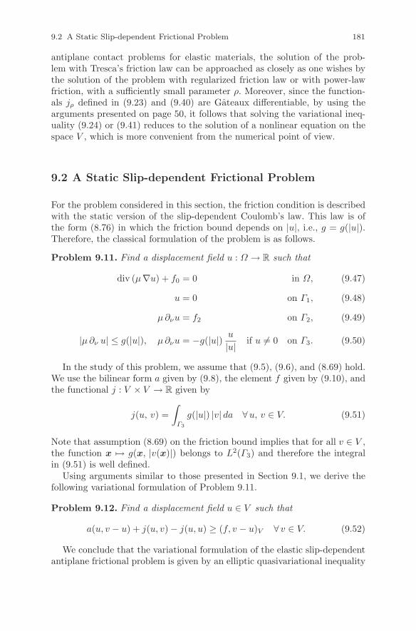
9.2 A Static Slip-dependent Frictional Problem 181
antiplane contact problems for elastic materials, the solution of the prob-lem with Tresca’s friction law can be approached as closely as one wishes bythe solution of the problem with regularized friction law or with power-lawfriction, with a sufficiently small parameter ρ. Moreover, since the function-als jρ defined in (9.23) and (9.40) are Gateaux differentiable, by using thearguments presented on page 50, it follows that solving the variational ineq-uality (9.24) or (9.41) reduces to the solution of a nonlinear equation on thespace V , which is more convenient from the numerical point of view.
9.2 A Static Slip-dependent Frictional Problem
For the problem considered in this section, the friction condition is describedwith the static version of the slip-dependent Coulomb’s law. This law is ofthe form (8.76) in which the friction bound depends on |u|, i.e., g = g(|u|).Therefore, the classical formulation of the problem is as follows.
Problem 9.11. Find a displacement field u : Ω → R such that
div (µ∇u) + f0 = 0 in Ω, (9.47)
u = 0 on Γ1, (9.48)
µ ∂νu = f2 on Γ2, (9.49)
|µ ∂ν u| ≤ g(|u|), µ ∂νu = −g(|u|) u
|u| if u = 0 on Γ3. (9.50)
In the study of this problem, we assume that (9.5), (9.6), and (8.69) hold.We use the bilinear form a given by (9.8), the element f given by (9.10), andthe functional j : V × V → R given by
j(u, v) =
∫
Γ3
g(|u|) |v| da ∀u, v ∈ V. (9.51)
Note that assumption (8.69) on the friction bound implies that for all v ∈ V ,the function x → g(x, |v(x)|) belongs to L2(Γ3) and therefore the integralin (9.51) is well defined.
Using arguments similar to those presented in Section 9.1, we derive thefollowing variational formulation of Problem 9.11.
Problem 9.12. Find a displacement field u ∈ V such that
a(u, v − u) + j(u, v) − j(u, u) ≥ (f, v − u)V ∀ v ∈ V. (9.52)
We conclude that the variational formulation of the elastic slip-dependentantiplane frictional problem is given by an elliptic quasivariational inequality

182 9 Elastic Problems
and, therefore, we turn to the results presented in Section 3.3 to solve thisproblem.
Our first result in the study of Problem 9.12 is the following.
Theorem 9.13. Assume that (9.5), (9.6), and (8.69) hold. Then there existsa constant L0, which depends only on Ω, Γ1, Γ3, and µ, such that problem(9.52) has a unique solution u that depends Lipschitz continuously on f , ifLg < L0.
Proof. For all η ∈ V , the functional j(η, ·) : V → R is a continuous seminormand therefore is convex and l.s.c., i.e., it satisfies (3.30)(a). Let u1, u2, v1,v2 ∈ V ; by using (9.51) and (8.69), we find that
j(u1, v2) − j(u1, v1) + j(u2, v1) − j(u2, v2)
=
∫
Γ3
(g(|u1|) − g(|u2|)
)(|v2| − |v1|) da
≤∫
Γ3
Lg|u1 − u2| |v1 − v2| da
≤ Lg‖u1 − u2‖L2(Γ3) ‖v1 − v2‖L2(Γ3)
and, keeping in mind (8.33), we obtain
j(u1, v2) − j(u1, v1) + j(u2, v1) − j(u2, v2)
≤ c20 Lg ‖u1 − u2‖V ‖v1 − v2‖V . (9.53)
Let
L0 =µ∗
c20
. (9.54)
Clearly, L0 depends only on Ω, Γ1, Γ3, and µ. It follows from (9.53) thatj satisfies condition (3.30)(b) with α = c2
0 Lg and, moreover, it follows from(8.52) that a satisfies condition (3.2) with m = µ∗. Assume now that Lg < L0;then we obtain c2
0 Lg < µ∗, which implies that m > α. Theorem 9.13 followsnow from Theorem 3.7 on page 51. ⊓⊔
We conclude by Theorem 9.13 that, under a smallness assumption on Lg,Problem 9.12 has a unique weak solution that depends Lipschitz continuouslyon the data.
We now prove the existence of a solution to the quasivariational inequality(9.52) without any smallness assumption on Lg.
Theorem 9.14. Assume that (9.5), (9.6), and (8.69) hold. Then there existsat least one solution to Problem 9.12.

9.3 Quasistatic Frictional Problems 183
Proof. We use Theorem 3.10. To this end, we note that the functional jgiven by (9.51) satisfies condition (3.36). Let us now consider the sequencesηn ⊂ V, un ⊂ V such that ηn η ∈ V and un u ∈ V. Using thecompactness property of the trace operator and (8.69), we obtain that
g(|ηn|) → g(|η|) in L2(Γ3),
|un| → |u| in L2(Γ3).
Therefore, by the definition of the functional j, we deduce that
j(ηn, v) → j(η, v) ∀ v ∈ V,
j(ηn, un) → j(η, u),
which show that the functional j satisfies condition (3.37). Finally, recallthat V is a separable Hilbert space, as proved in Theorem 8.1. Theorem 9.14follows now from Theorem 3.10 on page 53. ⊓⊔
Note that Theorem 3.10 can be used to prove the uniqueness of the solutionof Problem 9.12 and its Lipschitz continuous dependence on the data underthe smallness assumption in Theorem 9.13. Indeed, we choose u1 = v1 = uand u2 = v2 = v in (9.53) to obtain that
j(u, v) − j(u, u) + j(v, u) − j(u, u) ≤ c20 Lg ‖u − v‖2
V
and, choosing Lg < L0 with L0 given by (9.54), we deduce that j satisfiescondition (3.39). We conclude by Theorem 3.10 (3) that, if Lg < L0, then thesolution of Problem 9.12 is unique and depends Lipschitz continuously on f.
9.3 Quasistatic Frictional Problems
In this section, we study the quasistatic versions of the first two frictionalcontact problems presented in Section 9.1. We apply the results presented inSections 5.1 and 5.2 to prove the existence of a unique weak solution to eachone of these problems.
To construct the quasistatic version of Problem 9.1, we consider a timeinterval of interest [0, T ] with T > 0, allow the body forces and tractionsto depend on time, replace (9.4) with the evolutionary version of Tresca’sfriction law, (8.60), and add an initial condition for the displacement field.Therefore, the problem can be formulated as follows.
Problem 9.15. Find a displacement field u : Ω × [0, T ] → R such that
div (µ∇u) + f0 = 0 in Ω × (0, T ), (9.55)
u = 0 on Γ1 × (0, T ), (9.56)
µ ∂νu = f2 on Γ2 × (0, T ), (9.57)

184 9 Elastic Problems
|µ ∂ν u| ≤ g, µ ∂νu = −gu
|u| if u = 0 on Γ3 × (0, T ), (9.58)
u(0) = u0 in Ω. (9.59)
In the study of this problem, we assume that the Lame coefficient µ andthe friction bound g satisfy condition (9.6) and (9.7), respectively; moreover,we assume that the body forces and surface tractions satisfy
f0 ∈ W 1,2(0, T ;L2(Ω)), f2 ∈ W 1,2(0, T ;L2(Γ2)). (9.60)
We use notation (9.8) and (9.9) for the bilinear form a and the func-tional j; also, we use Riesz’s representation theorem to define the functionf : [0, T ] → V by the equality
(f(t), v)V =
∫
Ω
f0(t) v dx +
∫
Γ2
f2(t) v da ∀ v ∈ V, t ∈ [0, T ]. (9.61)
It follows from (9.60) that the integrals in (9.61) are well defined and,moreover,
f ∈ W 1,2(0, T ;V ). (9.62)
Finally, we assume that the initial displacement u0 satisfies
u0 ∈ V, (9.63)
a(u0, v) + j(v) ≥ (f(0), v)V ∀ v ∈ V. (9.64)
Condition (9.64) represents a compatibility condition on the initial data thatis necessary in many quasistatic problems, see for instance [130]. Physically,it is needed so as to guarantee that initially the state is in equilibrium, sinceotherwise the inertial terms cannot be neglected and the problems becomedynamic.
Proceeding as in the case of the static problem 9.1, we obtain the followingvariational formulation of the contact problem (9.55)–(9.59).
Problem 9.16. Find a displacement field u : [0, T ] → V such that
a(u(t), v − u(t)) + j(v) − j(u(t))
≥ (f(t), v − u(t))V ∀ v ∈ V, a.e. t ∈ (0, T ), (9.65)
u(0) = u0. (9.66)
We conclude that the variational formulation of the quasistatic prob-lem 9.15 is given by an evolutionary variational inequality and, therefore,we prove the unique solvability of Problem 9.16 by using the regularizationmethod presented in Section 5.2. The interest in this method arises fromthe fact that it is constructive, i.e., it provides the existence of the solution

9.3 Quasistatic Frictional Problems 185
by passing to the limit in a sequence of regularized problems. We start byconsidering the following problem, for ρ > 0.
Problem 9.17. Find a displacement field uρ : Ω × [0, T ] → R such that
div (µ∇uρ) + f0 = 0 in Ω × (0, T ), (9.67)
uρ = 0 on Γ1 × (0, T ), (9.68)
µ ∂νuρ = f2 on Γ2 × (0, T ), (9.69)
µ ∂νuρ = −guρ√
u2ρ + ρ2
on Γ3 × (0, T ), (9.70)
uρ(0) = u0 in Ω. (9.71)
Note that Problem 9.17 represents the quasistatic version of Problem 9.4,page 174. Also, it represents a regularization of Problem 9.15 since it is obt-ained from this last problem by replacing the Tresca friction law (9.58) withits regularization (9.70).
In the study of this problem, we assume that (9.6), (9.7), (9.60), (9.63),and (9.64) hold. Proceeding as in the case of the static problem 9.4, byusing notation (9.8), (9.23), and (9.61) we obtain the following variationalformulation of the contact problem (9.67)–(9.71).
Problem 9.18. Find a displacement field uρ : [0, T ] → V such that
a(uρ(t), v − uρ(t)) + jρ(v) − jρ(uρ(t))
≥ (f(t), v − uρ(t))V ∀ v ∈ V, a.e. t ∈ (0, T ), (9.72)
u(0) = u0. (9.73)
We have the following existence, uniqueness, and convergence result.
Theorem 9.19. Assume conditions (9.6), (9.7), (9.60), (9.63), and (9.64).Then:
(1) For each ρ > 0, there exists a unique solution to Problem 9.18 and itsatisfies uρ ∈ W 1,2(0, T ;V ).
(2) There exists a unique solution to Problem 9.16 and it satisfies u ∈W 1,2(0, T ;V ).
(3) The solution uρ of Problem 9.18 converges to the solution u of Problem9.16, i.e.,
uρ → u in C([0, T ], V ) as ρ → 0. (9.74)
Proof. We use Theorem 5.11. To this end, we note that the bilinear form a issymmetric, and it follows from (9.6) that it is continuous and V -elliptic, i.e., itsatisfies condition (5.3). Next, (9.62)–(9.64) show that conditions (5.5)–(5.7)

186 9 Elastic Problems
are satisfied, the last one with δ0 = 0. Recall that, as seen in the proof ofTheorem 9.3, j is a continuous seminorm on V and satisfies (9.15); there-fore, we conclude that j satisfies condition (5.63). Finally, it follows fromLemma 9.7 that conditions (5.64) and (3.17) hold, too. Thus, Theorem 9.19is a direct consequence of Theorem 5.11, which completes the proof. ⊓⊔
We conclude by Theorem 9.19 that problems 9.15 and 9.17 have a uniqueweak solution. Also, the weak solution of the quasistatic contact problemwith Tresca’s friction law can be approached by the weak solution of thequasistatic contact problem with regularized friction law for a sufficientlysmall parameter ρ.
Finally, note that if we replace condition (9.60) with the condition
f0 ∈ W 1,∞(0, T ;L2(Ω)), f2 ∈ W 1,∞(0, T ;L2(Γ2)), (9.75)
then the solution u of Problem 9.15 has the regularity u ∈ W 1,∞(0, T ;V ).Indeed, note that (9.75) implies that the element f given by (9.61) satis-fies f ∈ W 1,∞(0, T ;V ) and, since j is a continuous seminorm, the existenceof a unique solution u ∈ W 1,∞(0, T ;V ) to Problem 9.15 follows now fromCorollary 5.20. And we also note that in this case, the solution dependsLipschitz continuously on the data f0, f2, and u0 since, using again Corol-lary 5.20, it follows that the mapping (f, u0) → u is Lipschitz continuousfrom W 1,∞(0, T ;V ) × V to C([0, T ];V ).
9.4 A Quasistatic Slip-dependent Frictional Problem
In this section, we study the quasistatic version of the slip-dependent fric-tional contact problem presented in Section 9.2. We show that the problemleads to an evolutionary quasivariational inequality for the displacement fieldand therefore we apply Theorem 5.15 to prove its weak solvability.
The classical formulation of the problem is the following.
Problem 9.20. Find a displacement field u : Ω × [0, T ] → R such that
div (µ∇u) + f0 = 0 in Ω × (0, T ), (9.76)
u = 0 on Γ1 × (0, T ), (9.77)
µ ∂νu = f2 on Γ2 × (0, T ), (9.78)
|µ ∂νu| ≤ g(|u|), µ ∂νu = −g(|u|) u
|u| if u = 0 on Γ3 × (0, T ), (9.79)
u(0) = u0 in Ω. (9.80)
In the study of this problem, we assume that the Lame coefficient µ satisfiescondition (9.6) and the friction bound g satisfies condition (8.69); moreover,

9.4 A Quasistatic Slip-dependent Frictional Problem 187
the body forces and surface tractions satisfy
f0 ∈ W 1,∞(0, T ;L2(Ω)), f2 ∈ W 1,∞(0, T ;L2(Γ2)). (9.81)
We use notation (9.8) for the bilinear form a, (9.51) for the functional j, and(9.61) for the function f . It follows from (9.81) that
f ∈ W 1,∞(0, T ;V ). (9.82)
Finally, we assume that the initial displacement u0 satisfies
u0 ∈ V, (9.83)
a(u0, v) + j(u0, v) ≥ (f(0), v)V ∀ v ∈ V, (9.84)
and we recall that (9.84) represents a compatibility condition on the ini-tial data that is necessary to guarantee that initially the elastic body is inequilibrium.
Proceeding as in the case of the static problem 9.1, we obtain the followingvariational formulation of the contact problem (9.76)–(9.80).
Problem 9.21. Find a displacement field u : [0, T ] → V such that
a(u(t), v − u(t)) + j(u(t), v) − j(u(t), u(t))
≥ (f(t), v − u(t))V ∀ v ∈ V, a.e. t ∈ (0, T ), (9.85)
u(0) = u0. (9.86)
In the study of Problem 9.21, we have the following existence result.
Theorem 9.22. Assume that conditions (9.6), (9.81), (9.83), (9.84), and(8.69) hold. Then there exists L0 that depends only on Ω, Γ1, Γ3, and µsuch that there exists at least one solution u for Problem 9.21 that satisfiesu ∈ W 1,∞(0, T ;V ), if Lg < L0.
Proof. The bilinear form a is symmetric, and recall that it satisfies the inequa-lities (8.51) and (8.52), i.e., is continuous and V -elliptic. It also follows from(9.51) that for all η ∈ V , j(η, ·) is a continuous seminorm on V and, as it wasshown in the proof of Theorem 9.14, it satisfies condition (5.101).
Let u, v ∈ V ; by using (9.51) and (8.69) we find that
j(u, v − u) − j(v, v − u) =
∫
Γ3
(g(|u|) − g(|v|)
)|v − u| da
≤∫
Γ3
Lg|u − v|2 da ≤ Lg‖u − v‖2L2(Γ3)
and, therefore, by (8.33) we obtain
j(u, v − u) − j(v, v − u) ≤ c20 Lg ‖u − v‖2
V . (9.87)

188 9 Elastic Problems
Let L0 be defined by (9.54). Clearly, L0 depends only on Ω, Γ1, Γ3, and µ. Itfollows from (9.87) that j satisfies the inequality in (5.102) with α = c2
0 Lg,and it follows from (8.52) that a satisfies condition (5.3)(b) with m = µ∗.Assume that Lg < L0; then, we obtain
c20 Lg < µ∗ (9.88)
and we conclude by (9.87) that j satisfies condition (5.102).
Let now η, u ∈ V ; it follows from (9.51), (8.69), and (8.33) that
|j(η, u)| ≤∫
Γ3
(Lg|η| + g(0)
)|u| da
≤(Lg‖η‖L2(Γ3) + ‖g(0)‖L2(Γ3)
)‖u‖L2(Γ3)
≤ c0
(c0Lg‖η‖V + ‖g(0)‖L2(Γ3)
)‖u‖V .
We use the inequality
ab ≤ c
2a2 +
1
2cb2 ∀ a, b, c > 0
with a = c0
(c0Lg‖η‖V + ‖g(0)‖L2(Γ3)
), b = ‖u‖V , and c > 0 to find that
j(η, u) ≤ c
2c20
(c0Lg‖η‖V + ‖g(0)‖L2(Γ3)
)2+
1
2c‖u‖2
V . (9.89)
We now choose c such that
c >1
2(µ∗ − c20Lg)
(9.90)
and we recall that this choice is allowed by (9.88). Inequality (9.89) showsthat (5.103) holds with a1, a2 : V → R given by
a1(η) =1
2c, a2(η) =
c
2c20
(c0Lg‖η‖V + ‖g(0)‖L2(Γ3)
)2,
as by (9.90) we have a1(0V ) = 12c < µ∗ − c2
0Lg.
Let now ηn ⊂ V be such that ηn η ∈ V and let un ⊂ V be abounded sequence, that is, there exists c > 0 such that
‖un‖V ≤ c ∀n ∈ N. (9.91)
We use (9.51), (8.69), and (8.33) to find that
|j(ηn, un) − j(η, un)| ≤ c0Lg‖ηn − η‖L2(Γ3)‖un‖V ∀n ∈ N. (9.92)

9.4 A Quasistatic Slip-dependent Frictional Problem 189
Using the compactness property of the trace map, it follows that
‖ηn − η‖L2(Γ3) → 0. (9.93)
We combine now (9.91)–(9.93) to see that j satisfies condition (5.104).We conclude that a and j satisfy conditions (5.3), (5.100)–(5.104) of
Theorem 5.15 and we recall that V is a separable Hilbert space. Therefore,since (9.82)–(9.84) hold, it follows from Theorem 5.15(1) that there exists atleast a solution u ∈ W 1,∞(0, T ;V ) to Problem 9.21. ⊓⊔
Theorem 9.22 shows the solvability of the Problem 9.21, if the Lipschitzconstant Lg is small enough. Using (9.54), it follows that the critical valueL0 = µ
c20
(where c0 is defined on page 153) depends only on Ω, Γ1, Γ3, and µ,
and does not depend on the other data of the problem. Note that the criticalvalue L0 in Theorems 9.13 and 9.22 is the same. However, its significance inthe theorems above is different. Indeed, the existence of a weak solution forthe static antiplane slip-dependent frictional contact problem 9.12 is guar-anteed by Theorem 9.14 and, as it results from Theorem 9.13, the smallnessassumption Lg < L0 represents a sufficient condition to derive its uniqueness.The situation is different concerning the quasistatic antiplane slip-dependentfrictional contact problem 9.21 since Lg < L0 represents a sufficient conditionto derive the existence of the weak solution, see Theorem 9.22. The questionif this smallness assumption represents an intrinsic feature of the above an-tiplane contact problems or represents only a limitation of our mathematicaltools is left open and, clearly, it needs further investigation in the future.

Chapter 10
Viscoelastic Problems with Short Memory
In this chapter, we study quasistatic models for antiplane frictional problemsinvolving viscoelastic materials with short memory. We model the frictionwith versions of Coulomb’s law, including Tresca’s law and its regularization,slip-dependent and total slip-dependent laws. For all the models, we provethat the displacement field satisfies an evolutionary variational inequalitywith viscosity. Then we apply the results in Chapter 4 to obtain existence,uniqueness, regularity, and convergence results. In this chapter, we use againthe space V (page 152), together with its inner product (·, ·)V and the asso-ciated norm ‖ · ‖V . Moreover, [0, T ] represents the time interval of interest,T > 0. Finally, we note that everywhere in this chapter, the use of theabstract results presented in Part II of this book is made in the case X = V ,(·, ·)X = (·, ·)V , without explicit specification.
10.1 Problems with Tresca and Regularized Friction
For the first antiplane frictional contact problem we consider in this section,the friction is modeled with Tresca’s law and, therefore, the classical modelof the process is the following.
Problem 10.1. Find a displacement field u : Ω × [0, T ] → R such that
div (θ ∇u + µ∇u) + f0 = 0 in Ω × (0, T ), (10.1)
u = 0 on Γ1 × (0, T ), (10.2)
θ ∂ν u + µ ∂νu = f2 on Γ2 × (0, T ), (10.3)
|θ ∂ν u + µ ∂νu| ≤ g,θ ∂ν u + µ ∂νu = −g u
|u| if u = 0
on Γ3 × (0, T ), (10.4)
u(0) = u0 in Ω. (10.5)
191

192 10 Viscoelastic Problems with Short Memory
Note that (10.1) represents the equation of equilibrium (8.11), (10.2) rep-resents the displacement boundary condition (8.16), (10.3) represents thesurface traction boundary condition (8.24), (10.4) represents the Tresca fric-tion law (8.61), and, finally, (10.5) represents the initial condition. Note alsothat with respect to the quasistatic antiplane problem with Tresca’s fric-tion law treated in Section 9.3, the equilibrium equation (10.1) as well asthe boundary conditions (10.3) and (10.4) contain now an additional terminvolving the viscosity coefficient θ; this term arises from the fact that herewe use the viscoelastic constitutive law with short memory instead of theelastic constitutive law used everywhere in Chapter 9.
In the study of Problem 10.1, we assume that the elasticity and theviscosity coefficients satisfy
µ ∈ L∞(Ω), (10.6)
θ ∈ L∞(Ω), and there exists θ∗ > 0
such that θ(x) ≥ θ∗ a.e. x ∈ Ω. (10.7)
The body forces and surface tractions densities satisfy
f0 ∈ C([0, T ];L2(Ω)), f2 ∈ C([0, T ];L2(Γ2)), (10.8)
the friction bound g satisfies
g ∈ L2(Γ3) and g(x) ≥ 0 a.e. x ∈ Γ3, (10.9)
and, finally, the initial displacement is such that
u0 ∈ V. (10.10)
We define the bilinear forms a : V × V → R, b : V × V → R and thefunctional j : V → R by the equalities
a(u, v) =
∫
Ω
µ∇u · ∇v dx ∀u, v ∈ V, (10.11)
b(u, v) =
∫
Ω
θ ∇u · ∇v dx ∀u, v ∈ V, (10.12)
j(v) =
∫
Γ3
g|v| da ∀ v ∈ V, (10.13)
and we note that by assumptions (10.6)–(10.7) and (10.9), the integrals in(10.11)–(10.13) are well defined. We also use (10.8) and the Riesz representa-tion theorem (page 11) to define the function f : [0, T ] → V by the equality
(f(t), v)V =
∫
Ω
f0(t) v dx +
∫
Γ2
f2(t) v da ∀ v ∈ V, t ∈ [0, T ]. (10.14)
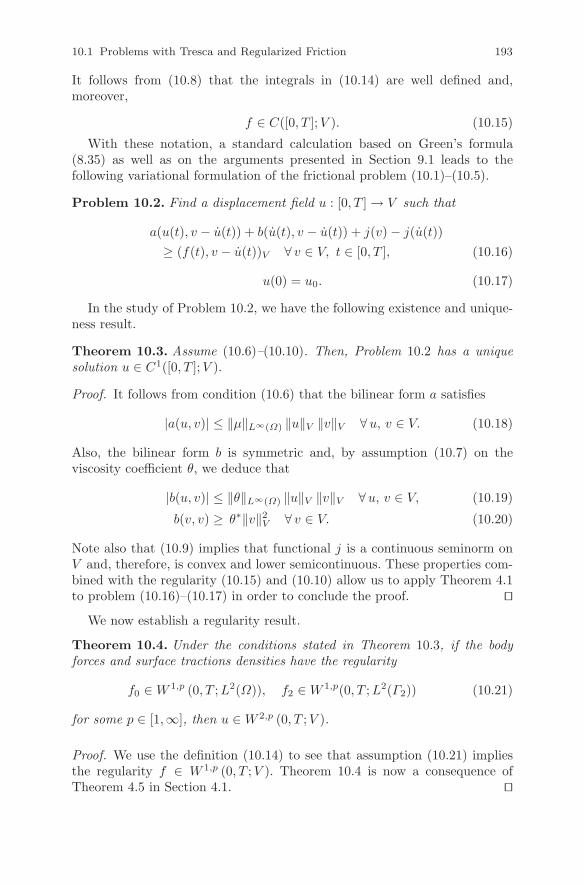
10.1 Problems with Tresca and Regularized Friction 193
It follows from (10.8) that the integrals in (10.14) are well defined and,moreover,
f ∈ C([0, T ];V ). (10.15)
With these notation, a standard calculation based on Green’s formula(8.35) as well as on the arguments presented in Section 9.1 leads to thefollowing variational formulation of the frictional problem (10.1)–(10.5).
Problem 10.2. Find a displacement field u : [0, T ] → V such that
a(u(t), v − u(t)) + b(u(t), v − u(t)) + j(v) − j(u(t))
≥ (f(t), v − u(t))V ∀ v ∈ V, t ∈ [0, T ], (10.16)
u(0) = u0. (10.17)
In the study of Problem 10.2, we have the following existence and unique-ness result.
Theorem 10.3. Assume (10.6)–(10.10). Then, Problem 10.2 has a uniquesolution u ∈ C1([0, T ];V ).
Proof. It follows from condition (10.6) that the bilinear form a satisfies
|a(u, v)| ≤ ‖µ‖L∞(Ω) ‖u‖V ‖v‖V ∀u, v ∈ V. (10.18)
Also, the bilinear form b is symmetric and, by assumption (10.7) on theviscosity coefficient θ, we deduce that
|b(u, v)| ≤ ‖θ‖L∞(Ω) ‖u‖V ‖v‖V ∀u, v ∈ V, (10.19)
b(v, v) ≥ θ∗‖v‖2V ∀ v ∈ V. (10.20)
Note also that (10.9) implies that functional j is a continuous seminorm onV and, therefore, is convex and lower semicontinuous. These properties com-bined with the regularity (10.15) and (10.10) allow us to apply Theorem 4.1to problem (10.16)–(10.17) in order to conclude the proof. ⊓⊔
We now establish a regularity result.
Theorem 10.4. Under the conditions stated in Theorem 10.3, if the bodyforces and surface tractions densities have the regularity
f0 ∈ W 1,p (0, T ;L2(Ω)), f2 ∈ W 1,p(0, T ;L2(Γ2)) (10.21)
for some p ∈ [1,∞], then u ∈ W 2,p (0, T ;V ).
Proof. We use the definition (10.14) to see that assumption (10.21) impliesthe regularity f ∈ W 1,p (0, T ;V ). Theorem 10.4 is now a consequence ofTheorem 4.5 in Section 4.1. ⊓⊔

194 10 Viscoelastic Problems with Short Memory
We conclude by Theorem 10.3 that the mechanical problem 10.1 has aunique weak solution. The regularity of the solution is higher than the reg-ularity of the data, since if f0 and f2 are continuous, then the solution uis continuously differentiable, and if f0 and f2 are W 1,p functions, then thesolution u is a W 2,p function, as derived in Theorem 10.4. This feature arisesfrom the structure of the problem that involves a new bilinear form, b, inwhich the derivative u of the solution plays the main role. Note also that,in comparison with Theorem 9.19, Theorems 10.3 and 10.4 provide a betterregularity result, under a less restrictive assumption on the Lame coefficientµ and on the initial displacement u0 (compare (9.6) with (10.6) and (9.63)–(9.64) with (10.10), respectively). We conclude that adding viscosity has asmoothing effect on the solution of antiplane frictional contact problems.
We now consider the viscoelastic problem with regularized friction. Theclassical formulation of the problem is as follows.
Problem 10.5. Find a displacement field uρ : Ω × [0, T ] → R such that
div (θ ∇uρ + µ∇uρ) + f0 = 0 in Ω × (0, T ), (10.22)
uρ = 0 on Γ1 × (0, T ), (10.23)
θ ∂ν uρ + µ ∂νuρ = f2 on Γ2 × (0, T ), (10.24)
θ ∂ν uρ + µ ∂νuρ = −guρ√
u2ρ + ρ2
on Γ3 × (0, T ), (10.25)
uρ(0) = u0 in Ω. (10.26)
This is the viscoelastic version of the quasistatic elastic problem 9.17,studied in Section 9.3. In the study of this problem, we assume that (10.6)–(10.10) hold and, moreover, ρ > 0. We use notation (10.11), (10.12), and(10.14) above and we introduce the frictional functional jρ : V → R given by
jρ(v) =
∫
Γ3
g(√
v2 + ρ2 − ρ)
da ∀ v ∈ V. (10.27)
Then, the variational formulation of the mechanical problem 10.5 is thefollowing.
Problem 10.6. Find a displacement field uρ : [0, T ] → V such that
a(uρ(t), v − uρ(t)) + b(uρ(t), v − uρ(t)) + jρ(v) − jρ(uρ(t))
≥ (f(t), v − uρ(t))V ∀ v ∈ V, t ∈ [0, T ], (10.28)
u(0) = u0. (10.29)
It follows from Lemma 9.7 and Corollary 1.37 (page 14) that jρ is a convexl.s.c. functional on V and jρ and j satisfy condition (3.17). Therefore, usingagain Theorems 4.1, 4.5, and 4.6, we obtain the following result.

10.2 Approach to Elasticity 195
Theorem 10.7. Assume (10.6)–(10.10). Then, for every ρ > 0, Problem 10.6has a unique solution uρ ∈ C1([0, T ];V ), and uρ ∈ W 2,p(0, T ;V ) if (10.21)holds. Moreover, the solution converges to the solution u of Problem 10.2, i.e.,
‖uρ − u‖C1([0,T ];V ) → 0 as ρ → 0. (10.30)
We conclude by Theorem 10.7 that the antiplane frictional problem(10.22)–(10.26) has a unique weak solution that converges to the weak solu-tion of Problem 10.1 as ρ → 0. In addition to the interest from the asymptoticpoint of view, this result is important from the mechanical point of view sinceit shows that, in the study of antiplane frictional contact problems for vis-coelastic materials with short memory, the solution of the problem with theTresca friction law can be approached as closely as one wishes by the solu-tion of the problem with regularized friction law with a sufficiently smallparameter ρ. Moreover, since the functional jρ defined in (10.27) is Gateauxdifferentiable, by using the arguments presented on page 67 it follows thatsolving the variational inequality (10.28)–(10.29) leads to the solution of aCauchy problem for nonlinear evolution equations on the space V , which isconvenient from the numerical point of view.
10.2 Approach to Elasticity
In this section, we investigate the behavior of the weak solution of the anti-plane frictional problems in Section 10.1 as the viscosity converges to zero.Our results below are valid both for the Tresca friction law and its regular-ization; however, to avoid repetitions, we restrict ourselves to the case of theTresca friction law. In order to outline the dependence on the viscosity coeffi-cient θ, we use in this section the notation bθ for the bilinear form (10.12), i.e.,
bθ(u, v) =
∫
Ω
θ ∇u · ∇v dx, ∀u, v ∈ V,
and reformulate Problem 10.2 as follows.
Problem 10.8. Find a displacement field uθ : [0, T ] → V such that
a(uθ(t), v − uθ(t)) + bθ(uθ(t), v − uθ(t)) + j(v) − j(uθ(t))
≥ (f(t), v − uθ(t))V ∀ v ∈ V, a.e. t ∈ (0, T ), (10.31)
uθ(0) = u0. (10.32)
We also consider the inviscid problem associated to (10.31)–(10.32), i.e.,the problem obtained for θ = 0. Note that this problem is the elastic frictional

196 10 Viscoelastic Problems with Short Memory
problem 9.16 studied in Section 9.3 and is formulated as follows.
Problem 10.9. Find a displacement field u : [0, T ] → V such that
a(u(t), v − u(t)) + j(v) − j(u(t))
≥ (f(t), v − u(t))V ∀ v ∈ V, a.e. t ∈ (0, T ), (10.33)
u(0) = u0. (10.34)
Assume in what follows that (9.6), (10.7), (10.9), (9.60), (9.63), and (9.64)hold. Then, it follows from Theorem 10.4 that Problem (10.31)–(10.32) hasa unique solution uθ ∈ W 2,2(0, T ;V ). It also follows from Theorem 9.19 thatproblem (10.33)–(10.34) has a unique solution u ∈ W 1,2(0, T ;V ). Considernow the assumption
1
θ∗ ‖θ‖2L∞(Ω) → 0. (10.35)
We have the following convergence result.
Theorem 10.10. Under the stated assumptions, if (10.35) holds, then thesolution uθ of Problem 10.8 converges to the solution u of Problem 10.9, i.e.,
‖uθ − u‖C([0,T ];V ) → 0. (10.36)
Proof. It follows from (10.19) and (10.20) that the bilinear form bθ satisfiescondition (5.88) with M ′(θ) = ‖θ‖L∞(Ω) and m′(θ) = θ∗. The convergenceresult (10.36) is now a consequence of Theorem 5.14. ⊓⊔
Consider now the case of homogeneous viscosity, i.e., the case when assum-ption (10.7) is replaced by the assumption
θ(x) = θ > 0 a.e. x ∈ Ω,
where θ is given. In this case, ‖θ‖L∞(Ω) = θ, θ∗ = θ and so the convergence(10.35) is equivalent to θ → 0. Therefore, by Theorem 10.10 we concludethat the weak solution of the antiplane viscoelastic problem with Tresca’sfriction law may be approached by the weak solution of the antiplane elasticproblem with Tresca’s friction law, as the viscosity is small enough. From themechanical point of view, this convergence result shows that the elasticitywith friction may be considered as a limit case of viscoelasticity with frictionas the viscosity decreases.
10.3 Slip- and Slip Rate–dependent Frictional Problems
In this section, we consider the frictional contact problem 10.1 in the casewhen the friction bound g depends on the slip |u| or on the slip rate |u|.

10.3 Slip- and Slip Rate–dependent Frictional Problems 197
The classical formulation of the problems follows in a straightforward wayfrom (10.1)–(10.5), by replacing g with g(|u|) or g(|u|), respectively. Thus,the antiplane viscoelastic contact problem with slip-dependent friction law isformulated as follows.
Problem 10.11. Find a displacement field u : Ω × [0, T ] → R such that
div (θ ∇u + µ∇u) + f0 = 0 in Ω × (0, T ), (10.37)
u = 0 on Γ1 × (0, T ), (10.38)
θ ∂ν u + µ ∂νu = f2 on Γ2 × (0, T ), (10.39)
|θ ∂ν u + µ ∂νu| ≤ g(|u|),θ ∂ν u + µ ∂νu = −g(|u|) u
|u| if u = 0
on Γ3 × (0, T ), (10.40)
u(0) = u0 in Ω. (10.41)
Also, the classical formulation of the antiplane viscoelastic contact problemwith slip rate–dependent friction law is as follows.
Problem 10.12. Find a displacement field u : Ω × [0, T ] → R such that
div (θ ∇u + µ∇u) + f0 = 0 in Ω × (0, T ), (10.42)
u = 0 on Γ1 × (0, T ), (10.43)
θ ∂ν u + µ ∂νu = f2 on Γ2 × (0, T ), (10.44)
|θ ∂ν u + µ ∂νu| ≤ g(|u|),θ ∂ν u + µ ∂νu = −g(|u|) u
|u| if u = 0
on Γ3 × (0, T ), (10.45)
u(0) = u0 in Ω. (10.46)
The variational formulation of Problem 10.11 can be obtained by usingthe arguments presented in Section 9.1 and is the following.
Problem 10.13. Find a displacement field u : [0, T ] → V such that
a(u(t), v − u(t)) + b(u(t), v − u(t)) + j(u(t), v) − j(u(t), u(t))
≥ (f(t), v − u(t))V ∀ v ∈ V, t ∈ [0, T ], (10.47)
u(0) = u0. (10.48)
Here and below in this section, we use notation (10.11) and (10.12) for thebilinear forms a and b as well as notation (10.14) for the function f . Also,

198 10 Viscoelastic Problems with Short Memory
the functional j : V × V → R is given by
j(u, v) =
∫
Γ3
g(|u|) |v| da ∀u, v ∈ V, (10.49)
where the friction bound g is assumed to satisfy (8.69).
The variational formulation of Problem 10.12 is the following.
Problem 10.14. Find a displacement field u : [0, T ] → V such that
a(u(t), v − u(t)) + b(u(t), v − u(t)) + j(u(t), v) − j(u(t), u(t))
≥ (f(t), v − u(t))V ∀ v ∈ V, t ∈ [0, T ], (10.50)
u(0) = u0. (10.51)
The well-posedness of the variational problems 10.13 and 10.14 is given bythe following existence and uniqueness result.
Theorem 10.15. Assume (10.6)–(10.8), (10.10), and (8.69). Then:(1) There exists a unique solution u ∈ C1([0, T ];V ) to problem (10.47)–
(10.48).(2) There exists L0, which depends on Ω, Γ1, Γ3, and θ, such that there
exists a unique solution u ∈ C1([0, T ];V ) to problem (10.50)–(10.51), ifLg < L0.
Proof. The bilinear form a, the function f , and the initial data u0 satisfyconditions (4.3), (4.6), and (4.7), respectively. In addition, for all η ∈ V ,the functional j(η, ·) : V → R is a continuous seminorm on V and thereforeit satisfies condition (3.30)(a). Recall also that j satisfies inequality (9.53)where c0 is given in (8.33), which shows that condition (3.30)(b) holds withα = c2
0 Lg. Moreover, it follows from (10.19) and (10.20) that the bilinear form
b satisfies condition (4.4) with m′ = θ∗. Choose L0 = θ∗
c20
, which depends on
Ω, Γ1, Γ3, and θ. Then, if Lg < L0 we have m′ > α, and therefore Theorem10.15 is a direct consequence of Theorem 4.7. ⊓⊔
It follows from Theorem 10.15 that the frictional viscoelastic problem withslip-dependent friction law has a unique weak solution and, under a small-ness assumption, the frictional viscoelastic problem with slip rate–dependentfriction law has a unique weak solution, too. Note also that the critical valueL0 depends only on the viscosity coefficient θ and on the geometry of theproblem, but does not depend on the Lame coefficient µ, the external forces,nor on the initial displacement.
Finally, we remark that if the body forces and surface tractions densitiessatisfy (10.21) for some p ∈ [1, ∞], then the solution of problems 10.13 and10.14 satisfies u ∈ W 2,p(0, T ;V ). Indeed, this regularity is a direct conse-quence of Theorem 4.8.
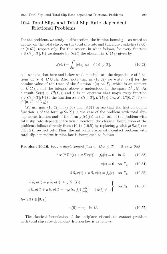
10.4 Total Slip- and Total Slip Rate–dependent Frictional Problems 199
10.4 Total Slip- and Total Slip Rate–dependentFrictional Problems
For the problems we study in this section, the friction bound g is assumed todepend on the total slip or on the total slip rate and therefore g satisfies (8.66)or (8.67), respectively. For this reason, in what follows, for every functionv ∈ C([0, T ];V ) we denote by Sv(t) the element in L2(Γ3) given by
Sv(t) =
∫ t
0
|v(s)| ds ∀ t ∈ [0, T ], (10.52)
and we note that here and below we do not indicate the dependence of func-tions on x ∈ Ω ∪ Γ3. Also, note that in (10.52) we write |v(s)| for theabsolue value of the trace of the function v(s) on Γ3, which is an elementof L2(Γ3), and the integral above is understood in the space L2(Γ3). Asa result Sv(t) ∈ L2(Γ3), and S is an operator that maps every functionv ∈ C([0, T ];V ) to the function Sv ∈ C([0, T ], L2(Γ3)), i.e., S : C([0, T ];V ) →C([0, T ], L2(Γ3)).
We use now (10.52) in (8.66) and (8.67) to see that the friction boundfunction is of the form g(Su(t)) in the case of the problem with total slip-dependent friction and of the form g(Su(t)) in the case of the problem withtotal slip rate–dependent friction. Therefore, the classical formulation of theproblems follows directly from (10.1)–(10.5) by replacing g with g(Su(t)) org(Su(t)), respectively. Thus, the antiplane viscoelastic contact problem withtotal slip-dependent friction law is formulated as follows.
Problem 10.16. Find a displacement field u : Ω × [0, T ] → R such that
div (θ ∇u(t) + µ∇u(t)) + f0(t) = 0 in Ω, (10.53)
u(t) = 0 on Γ1, (10.54)
θ ∂ν u(t) + µ ∂νu(t) = f2(t) on Γ2, (10.55)
|θ ∂ν u(t) + µ ∂νu(t)| ≤ g(Su(t)),
θ ∂ν u(t) + µ ∂νu(t) = −g(Su(t)) u(t)|u(t)| if u(t) = 0
on Γ3, (10.56)
for all t ∈ [0, T ],
u(0) = u0 in Ω. (10.57)
The classical formulation of the antiplane viscoelastic contact problemwith total slip rate–dependent friction law is as follows.

200 10 Viscoelastic Problems with Short Memory
Problem 10.17. Find a displacement field u : Ω × [0, T ] → R such that
div (θ ∇u(t) + µ∇u(t)) + f0(t) = 0 in Ω, (10.58)
u(t) = 0 on Γ1, (10.59)
θ ∂ν u(t) + µ ∂νu(t) = f2(t) on Γ2, (10.60)
|θ ∂ν u(t) + µ ∂νu(t)| ≤ g(Su(t)),
θ ∂ν u(t) + µ ∂νu(t) = −g(Su(t)) u(t)|u(t)| if u(t) = 0
on Γ3, (10.61)
for all t ∈ [0, T ],
u(0) = u0 in Ω. (10.62)
The variational formulation of Problem 10.16 can be obtained by usingthe arguments presented in Section 9.1 and is the following.
Problem 10.18. Find a displacement field u : [0, T ] → V such that
a(u(t), v − u(t)) + b(u(t), v − u(t)) + j(Su(t), v) − j(Su(t), u(t))
≥ (f(t), v − u(t))V ∀ v ∈ V, t ∈ [0, T ], (10.63)
u(0) = u0. (10.64)
Here and everywhere in this section, we use notation (10.11), (10.12),(10.14), and (10.52). Also, j : L2(Γ3) × V → R is the functional given by
j(η, v) =
∫
Γ3
g(η) |v| da ∀ η ∈ L2(Γ3), v ∈ V. (10.65)
The integral above exists under condition (8.69) on g, which we assume in thissection. We need to define j as above since at each time moment t ∈ [0, T ],the total slip Su(t) belongs to the space L2(Γ3). Considering the functional(10.65) instead of the functional (10.49) represents the first difference withrespect to the slip-dependent frictional problem studied in Section 10.3; thesecond difference consists in the fact that now the problem is history depen-dent since, unlike the functional j in Problem 10.13 that depends on thecurrent slip |u(t)|, the functional j in Problem 10.18 depends on the historyof the slip, Su(t).
Also, with the notation above, the variational formulation of Problem 10.17is as follows.
Problem 10.19. Find a displacement field u : [0, T ] → V such that
a(u(t), v − u(t)) + b(u(t), v − u(t)) + j(Su(t), v) − j(Su(t), u(t))
≥ (f(t), v − u(t))V ∀ v ∈ V, t ∈ [0, T ], (10.66)
u(0) = u0. (10.67)

10.4 Total Slip- and Total Slip Rate–dependent Frictional Problems 201
Again, note that considering the functional (10.65) instead of the func-tional (10.49) represents the first difference with respect to the slip rate–dependent frictional problem studied in Section 10.3; the second differenceconsists in the fact that now the problem is history dependent, since thefunctional j in Problem 10.19 depends on the history of the slip rate, Su(t).
The well-posedness of the variational problems 10.18 and 10.19 is given bythe following existence and uniqueness results.
Theorem 10.20. Assume (10.6)–(10.8), (10.10), and (8.69) then:(1) There exists a unique solution u ∈ C1([0, T ];V ) to problem (10.63)–
(10.64).(2) There exists a unique solution u ∈ C1([0, T ];V ) to problem (10.66)–
(10.67).
Proof. Conditions (10.6) and (10.7) imply that the bilinear forms a and b defi-ned by (10.11) and (10.12) satisfy assumptions (4.3) and (4.4), respectively;condition (8.69) on the friction bound g implies that the functional j givenby (10.65) satisfies assumption (3.54) with X = V and Y = L2(Γ3); also, itfollows from (10.52) that
‖Sv1(t) − Sv2(t)‖L2(Γ3)
≤∫ t
0
‖v1(s) − v2(s)‖L2(Γ3)ds ∀v1, v2 ∈ C([0, T ];V ), t ∈ [0, T ]
and, using (8.33), we deduce that S : C([0, T ];V ) → C([0, T ];L2(Γ3)) satisfiescondition (4.40) with X = V and Y = L2(Γ3); finally, recall the regularity(10.15) and (10.10), which shows that (4.6) and (4.7) also hold, respectively.Theorem 10.20 is now a consequence of Theorem 4.9 in Section 4.4. ⊓⊔
We conclude from Theorem 10.20 that the frictional viscoelastic problemwith total slip-dependent friction law and the frictional viscoelastic problemwith total slip rate–dependent friction law have, each one, a unique weaksolution that satisfies problems 10.18 and 10.19, respectively.
When compared with the result of Theorem 10.15(2), in Theorem 10.20(2)we do not need any smallness assumption on the friction bound g. The reasonlies in the structure of the corresponding problems: in Problem 10.14, thefunctional j depends on the current value of the derivative of the solution,u(t), whereas in Problem 10.19, the functional j depends on the solution viaan integral term, the total slip rate Su(t).
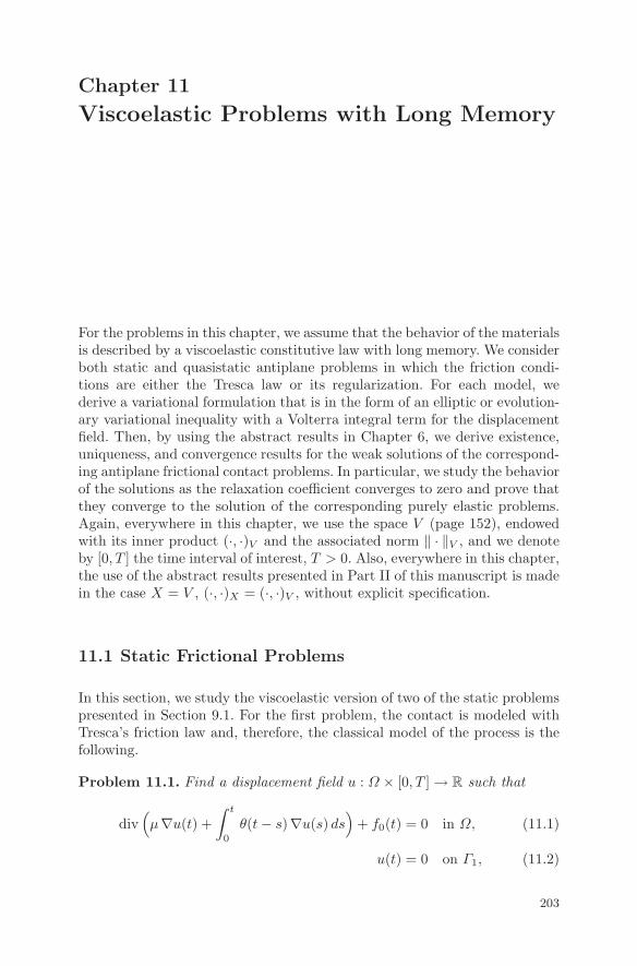
Chapter 11
Viscoelastic Problems with Long Memory
For the problems in this chapter, we assume that the behavior of the materialsis described by a viscoelastic constitutive law with long memory. We considerboth static and quasistatic antiplane problems in which the friction condi-tions are either the Tresca law or its regularization. For each model, wederive a variational formulation that is in the form of an elliptic or evolution-ary variational inequality with a Volterra integral term for the displacementfield. Then, by using the abstract results in Chapter 6, we derive existence,uniqueness, and convergence results for the weak solutions of the correspond-ing antiplane frictional contact problems. In particular, we study the behaviorof the solutions as the relaxation coefficient converges to zero and prove thatthey converge to the solution of the corresponding purely elastic problems.Again, everywhere in this chapter, we use the space V (page 152), endowedwith its inner product (·, ·)V and the associated norm ‖ · ‖V , and we denoteby [0, T ] the time interval of interest, T > 0. Also, everywhere in this chapter,the use of the abstract results presented in Part II of this manuscript is madein the case X = V , (·, ·)X = (·, ·)V , without explicit specification.
11.1 Static Frictional Problems
In this section, we study the viscoelastic version of two of the static problemspresented in Section 9.1. For the first problem, the contact is modeled withTresca’s friction law and, therefore, the classical model of the process is thefollowing.
Problem 11.1. Find a displacement field u : Ω × [0, T ] → R such that
div(µ∇u(t) +
∫ t
0
θ(t − s) ∇u(s) ds)
+ f0(t) = 0 in Ω, (11.1)
u(t) = 0 on Γ1, (11.2)
203

204 11 Viscoelastic Problems with Long Memory
µ∂ν u(t) +
∫ t
0
θ(t − s)∂νu(s) ds = f2(t) onΓ2, (11.3)
∣∣∣∣µ∂νu(t) +
∫ t
0
θ(t − s)∂νu(s) ds
∣∣∣∣ ≤ g,
µ∂νu(t) +
∫ t
0
θ(t − s)∂νu(s) ds
= −gu(t)
|u(t)| if u(t) = 0
on Γ3, (11.4)
for all t ∈ [0, T ].
Note that (11.1) represents the equation of equilibrium (8.15), (11.2) isthe displacement boundary condition (8.16), (11.3) represents the tractionboundary condition (8.25), and, finally, (11.4) represents the static versionof Tresca’s friction law, (8.62), in the case of viscoelastic materials with longmemory.
In the study of Problem 11.1, we assume that the elasticity and relaxationcoefficients satisfy
µ ∈ L∞(Ω) and there exists µ∗ > 0
such that µ(x) ≥ µ∗ a.e. x ∈ Ω, (11.5)
θ ∈ C([0, T ];L∞(Ω)). (11.6)
The body forces and surface tractions densities satisfy
f0 ∈ C([0, T ];L2(Ω)), f2 ∈ C([0, T ];L2(Γ2)), (11.7)
and, finally, the friction bound g satisfies
g ∈ L2(Γ3) and g(x) ≥ 0 a.e. x ∈ Γ3. (11.8)
We define the bilinear form a : V ×V → R and the functional j : V → R by
a(u, v) =
∫
Ω
µ∇u · ∇v dx ∀u, v ∈ V, (11.9)
j(v) =
∫
Γ3
g|v| da ∀ v ∈ V, (11.10)
and we note that by assumptions (11.5) and (11.8), the integrals in (11.9) and(11.10) are well defined. We also use (11.6), (11.7), and Riesz’s representationtheorem (page 11) to define the operator A : [0, T ] → L(V ) and the functionf : [0, T ] → V by the equalities
(A(t)u, v)V =
∫
Ω
θ(t) ∇u · ∇v dx ∀u, v ∈ V, t ∈ [0, T ], (11.11)
(f(t), v)V =
∫
Ω
f0(t) v dx +
∫
Γ2
f2(t) v da ∀ v ∈ V, t ∈ [0, T ]. (11.12)

11.1 Static Frictional Problems 205
It follows from (11.11), (11.12), and (8.32) that
‖A(t1) − A(t2)‖L(V ) ≤ ‖θ(t1) − θ(t2)‖L∞(Ω), (11.13)
‖f(t1) − f(t2)‖V ≤ c(‖f0(t1) − f0(t2)‖L2(Ω) + ‖f2(t1) − f2(t2)‖L2(Γ2)
)
(11.14)
for all t1, t2 ∈ [0, T ], and, keeping in mind (11.6) and (11.7), we deduce that
A ∈ C([0, T ];L(V )), (11.15)
f ∈ C([0, T ];V ). (11.16)
With this notation, a standard calculation based on Green’s formula (8.35)leads to the following variational formulation of the frictional problem (11.1)–(11.4).
Problem 11.2. Find a displacement field u : [0, T ] → V such that
a(u(t), v − u(t)) +
(∫ t
0
A(t − s) u(s) ds, v − u(t)
)
V
+ j(v) − j(u(t))
≥ (f(t), v − u(t))V ∀ v ∈ V, t ∈ [0, T ]. (11.17)
The difference between the variational model (11.17) and inequality (9.14)deduced in the study of the corresponding elastic problem arises in the factthat (11.17) involves the Volterra operator and the time variable, as well.
In the study of Problem 11.2, we have the following existence and unique-ness result.
Theorem 11.3. Assume that (11.5)–(11.8) hold. Then Problem 11.2 has aunique solution u ∈ C([0, T ];V ).
Proof. The bilinear form a is symmetric and, using the condition (11.5), wededuce
|a(u, v)| ≤ ‖µ‖L∞(Ω) ‖u‖V ‖v‖V ∀u, v ∈ V, (11.18)
a(v, v) ≥ µ∗ ‖v‖2V ∀ v ∈ V. (11.19)
Also, (11.8) implies that j is a continuous seminorm on V and, therefore,is a convex l.s.c. function. These properties combined with the regularity(11.15) and (11.16) allow us to apply Theorem 6.1 to conclude the proof ofTheorem 11.3. ⊓⊔
It follows from Theorem 11.3 that, under the assumptions stated above,the antiplane frictional problem 11.1 has a unique weak solution. We nowcomplete this existence and uniqueness result with the following regularityresult.

206 11 Viscoelastic Problems with Long Memory
Theorem 11.4. Under the conditions stated in Theorem 11.3, if there existsp ∈ [1,∞] such that
f0 ∈ W 1,p (0, T ;L2(Ω)), f2 ∈ W 1,p(0, T ;L2(Γ3)), (11.20)
θ ∈ W 1,p (0, T ;L∞(Ω)), (11.21)
then u ∈ W 1,p (0, T ;V ).
Proof. We use (11.14) to see that (11.20) implies f ∈ W 1,p (0, T ;V ). Also,it follows from (11.13) that (11.21) implies A ∈ W 1,p (0, T ;L(V )). Theorem11.4 is now a consequence of Theorem 6.3 in Section 6.1. ⊓⊔
We now consider the static viscoelastic problem with regularized friction.The classical formulation of the problem is as follows.
Problem 11.5. Find a displacement field uρ : Ω × [0, T ] → R such that
div
(µ∇uρ(t) +
∫ t
0
θ(t − s) ∇uρ(s) ds
)+ f0(t) = 0 in Ω, (11.22)
uρ(t) = 0 on Γ1, (11.23)
µ ∂νuρ(t) +
∫ t
0
θ(t − s) ∂νuρ(s) ds = f2(t) on Γ2, (11.24)
µ ∂νuρ(t) +
∫ t
0
θ(t − s) ∂νuρ(s) ds = −guρ(t)√
u2ρ(t) + ρ2
on Γ3, (11.25)
for all t ∈ [0, T ].
Note that Problem 11.5 represents a version of the elastic problem 9.4studied in Section 9.1, stated in the case of viscoelastic materials with longmemory.
In the study of Problem 11.5, we assume that (11.5)–(11.8) hold and,moreover, ρ > 0. Also, we define the functional jρ : V → R by
jρ(v) =
∫
Γ3
g(√
v2 + ρ2 − ρ)
da ∀ v ∈ V. (11.26)
With this notation, the variational formulation of the antiplane frictionalproblem 11.5 is the following.
Problem 11.6. Find a displacement field uρ : [0, T ] → V such that
a(uρ(t), v − uρ(t)) +
(∫ t
0
A(t − s) uρ(s) ds, v − uρ(t)
)
V
+ jρ(v) − jρ(uρ(t))
≥ (f(t), v − uρ(t))V ∀v ∈ V, t ∈ [0, T ]. (11.27)

11.2 Quasistatic Frictional Problems 207
Clearly, jρ is a convex lower semicontinuous function on V and, moreover,as it was shown in Lemma 9.7, jρ and j satisfy condition (3.17). Therefore,similar arguments as those used in the proof of Theorem 11.3, based on theabstract existence and uniqueness result provided by Theorem 6.1 combinedwith the regularity result in Theorem 6.3 and the abstract convergence resultin Theorem 6.10, lead to the following theorem.
Theorem 11.7. Assume (11.5)–(11.8). Then, for every ρ > 0, Problem 11.6has a unique solution uρ ∈ C[0, T ];V ), and uρ ∈ W 1,p(0, T ;V ) if (11.20)and (11.21) hold. Moreover, the solution converges to the solution u of Prob-lem 10.1, i.e.,
‖uρ − u‖C([0,T ];V ) → 0 as ρ → 0. (11.28)
We conclude by Theorem 11.7 that the antiplane frictional problem(11.22)–(11.25) has a unique weak solution that converges to the weak solu-tion of Problem 11.1 as ρ → 0. In addition to the mathematical interest inthis result, it is important from the mechanical point of view since it showsthat in the study of static frictional antiplane problems with viscoelasticmaterials with long memory, the solution of the problem with Tresca’s lawcan be approached as closely as one wishes by the solution of the problemwith regularized friction law with a sufficiently small parameter ρ.
11.2 Quasistatic Frictional Problems
In this section, we study the evolutionary versions of the models presented inSection 11.1. The difference arises in the fact that here we replace the staticfriction laws (11.4) and (11.25) with their evolutionary version (8.62) and(8.72), respectively, and, as a consequence, we need to prescribe an initialcondition for the displacement field. We start with the problem involving theTresca law; its classical formulation is the following.
Problem 11.8. Find a displacement field u : Ω × [0, T ] → R such that
div
(µ∇u(t) +
∫ t
0
θ(t − s) ∇u(s) ds
)+ f0(t) = 0 in Ω, (11.29)
u(t) = 0 on Γ1, (11.30)
µ ∂νu(t) +
∫ t
0
θ(t − s) ∂νu(s) ds = f2(t) on Γ2, (11.31)
∣∣∣∣µ∂νu(t) +
∫ t
0
θ(t − s)∂ν u(s) ds
∣∣∣∣ ≤ g,
µ ∂νu(t) +
∫ t
0
θ(t − s)∂νu(s) ds
= −gu(t)
|u(t)| if u(t) = 0
on Γ3, (11.32)

208 11 Viscoelastic Problems with Long Memory
for all t ∈ [0, T ],
u(0) = u0 in Ω. (11.33)
In the study of this problem, we assume that the Lame coefficient µ satisfies(11.5) and the friction bound g satisfies (11.8). We also assume that therelaxation coefficient θ has the regularity
θ ∈ W 1,2(0, T ;L∞(Ω)) (11.34)
and the body forces and surface tractions densities satisfy
f0 ∈ W 1,2 (0, T ;L2(Ω)), f2 ∈ W 1,2(0, T ;L2(Γ2)). (11.35)
Finally, we assume that the initial data satisfies
u0 ∈ V, (11.36)
a(u0, v) + j(v) ≥ (f(0), v) ∀ v ∈ V (11.37)
where, here and below, we use the notation (11.9)–(11.12). We note that(11.37) represents a compatibility condition for the initial displacement, alr-eady used in Section 9.3 in the study of quasistatic frictional problems withelastic materials.
The variational formulation of Problem 11.8 is the following.
Problem 11.9. Find a displacement field u : [0, T ] → V such that
a(u(t), v − u(t)) +
(∫ t
0
A(t − s) u(s) ds, v − u(t)
)
V
+ j(v) − j(u(t))
≥ (f(t), v − u(t))V ∀ v ∈ V, a.e. t ∈ (0, T ), (11.38)
u(0) = u0. (11.39)
The difference between the variational model (11.38)–(11.39) and the ineq-uality (11.17) deduced in the study of the corresponding static frictionalcontact problem arises from the fact that in (11.38)–(11.39), we use the testfunction v − u(t), and in (11.17), we use the test function v − u(t), where vis arbitrary in V . As a consequence, in Problem 11.9 we need to prescribean initial condition, (11.39), and (11.38)–(11.39) represents an evolutionaryvariational inequality.
In the study of Problem 11.9, we have the following existence and unique-ness result.
Theorem 11.10. Assume that (11.5), (11.8), (11.34)–(11.37) hold. Thenthere exists a unique solution to Problem 11.9 and, moreover, it satisfiesu ∈ W 1,2(0, T ;V ).

11.2 Quasistatic Frictional Problems 209
Proof. Using (11.5) and (11.8), it follows that the bilinear form a satisfiesassumption (6.2) and the functional j satisfies assumption (6.4). Next, com-bining (11.13) with (11.34), it follows that A ∈ W 1,2(0, T ;L(V )), and combin-ing (11.14) with (11.35), it follows that f ∈ W 1,2(0, T ;V ); thus, we concludethat the operator A and the function f satisfy conditions (6.14) and (6.15),respectively. Finally, we use (11.36) and (11.37) to see that conditions (6.16)and (6.17) are satisfied, too, the last one with δ0 = 0. Theorem 11.10 is nowa consequence of Theorem 6.4 on page 113. ⊓⊔
We conclude by Theorem 11.10 that the quasistatic frictional problem 11.1has a unique weak solution.
We consider now the quasistatic viscoelastic problem with regularized fric-tion. The classical formulation of the problem is as follows.
Problem 11.11. Find a displacement field uρ : Ω × [0, T ] → R such that
div
(µ∇uρ(t) +
∫ t
0
θ(t − s) ∇uρ(s) ds
)+ f0(t) = 0 in Ω, (11.40)
uρ(t) = 0 on Γ1, (11.41)
µ ∂νuρ(t) +
∫ t
0
θ(t − s) ∂νuρ(s) ds = f2(t) on Γ2, (11.42)
µ ∂νuρ(t) +
∫ t
0
θ(t − s) ∂νuρ(s) ds = −guρ(t)√
u2ρ(t) + ρ2
on Γ3, (11.43)
for all t ∈ [0, T ],uρ(0) = u0 in Ω. (11.44)
Note that Problem 11.11 represents a version of the elastic problem 9.17studied in Section 9.1, stated in the case of viscoelastic materials with longmemory.
In the study of Problem 11.11, we assume that (11.5), (11.8), (11.34)–(11.37) hold and, moreover, ρ > 0. Also, besides the notation already used inProblem 11.9, we use the notation (11.26) for the function jρ : V → R.
The variational formulation of the antiplane frictional Problem 11.11 isthe following.
Problem 11.12. Find a displacement field uρ : [0, T ] → V such that
a(uρ(t), v − uρ(t)) +
(∫ t
0
A(t − s) uρ(s) ds, v − uρ(t)
)
V
+ jρ(v) − jρ(uρ(t))
≥ (f(t), v − uρ(t))V ∀v ∈ V, a.e. t ∈ (0, T ), (11.45)
u(0) = u0. (11.46)

210 11 Viscoelastic Problems with Long Memory
Clearly, jρ is a convex lower semicontinuous function on V and, moreover,as was shown in the proof of Lemma 9.7, jρ and j satisfy condition (3.17).Therefore, similar arguments as those used in the proof of Theorem 11.10,based on the abstract existence and uniqueness result provided by Theo-rem 6.4 combined with the abstract convergence result in Theorem 6.11, leadto the following theorem.
Theorem 11.13. Assume (11.5), (11.8), (11.34)–(11.37). Then, for everyρ > 0, Problem 11.12 has a unique solution uρ ∈ W 1,2(0, T ;V ). Moreoverthe solution converges to the solution u of Problem 11.8, i.e.,
‖uρ − u‖C([0,T ];V ) → 0 as ρ → 0. (11.47)
We conclude by Theorem 11.13 that the antiplane frictional problem(11.40)–(11.44) has a unique weak solution that converges to the weak solu-tion of Problem 11.8 as ρ → 0. In addition to the mathematical interest inthis result, it is important from the mechanical point of view since it showsthat, in the study of quasistatic antiplane contact problems for viscoelasticmaterials with long memory, the solution of the problem with Tresca’s lawcan be approached as closely as one wishes by the solution of the contactproblem with regularized friction law with a sufficiently small parameter ρ.
11.3 Approach to Elasticity
In this section, we investigate the behavior of the weak solutions of the anti-plane frictional problems for viscoelastic materials with long memory as therelaxation coefficient converges to zero. We consider both the static and thequasistatic cases. Our results below are valid both for the Tresca friction lawand its regularization; however, to avoid repetition, we restrict ourselves tothe case of the Tresca friction law.
We start with the static case and, in order to outline the dependence ofthe solution on the given relaxation coefficient θ, we rewrite Problem 11.2 asfollows.
Problem 11.14. Find a displacement field uθ : [0, T ] → V such that
a(uθ(t), v − uθ(t)) +
(∫ t
0
Aθ(t − s) uθ(s) ds, v − uθ(t)
)
V
+ j(v) − j(uθ(t))
≥ (f(t), v − uθ(t))V ∀ v ∈ V, t ∈ [0, T ]. (11.48)
Here the operator Aθ is given by (11.11), i.e.,
(Aθ(t) u, v)V =
∫
Ω
θ(t) ∇u · ∇v dx ∀u, v ∈ V, t ∈ [0, T ]. (11.49)
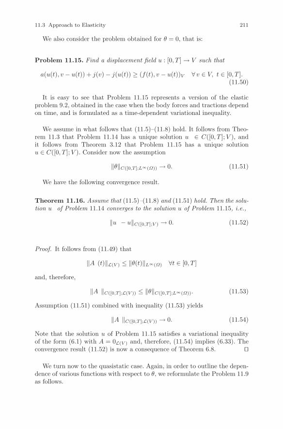
11.3 Approach to Elasticity 211
We also consider the problem obtained for θ = 0, that is:
Problem 11.15. Find a displacement field u : [0, T ] → V such that
a(u(t), v − u(t)) + j(v) − j(u(t)) ≥ (f(t), v − u(t))V ∀ v ∈ V, t ∈ [0, T ].(11.50)
It is easy to see that Problem 11.15 represents a version of the elasticproblem 9.2, obtained in the case when the body forces and tractions dependon time, and is formulated as a time-dependent variational inequality.
We assume in what follows that (11.5)–(11.8) hold. It follows from Theo-rem 11.3 that Problem 11.14 has a unique solution uθ ∈ C([0, T ];V ), andit follows from Theorem 3.12 that Problem 11.15 has a unique solutionu ∈ C([0, T ];V ). Consider now the assumption
‖θ‖C([0,T ];L∞(Ω)) → 0. (11.51)
We have the following convergence result.
Theorem 11.16. Assume that (11.5)–(11.8) and (11.51) hold. Then the solu-tion uθ of Problem 11.14 converges to the solution u of Problem 11.15, i.e.,
‖uθ − u‖C([0,T ];V ) → 0. (11.52)
Proof. It follows from (11.49) that
‖Aθ(t)‖L(V ) ≤ ‖θ(t)‖L∞(Ω) ∀t ∈ [0, T ]
and, therefore,
‖Aθ‖C([0,T ];L(V )) ≤ ‖θ‖C([0,T ];L∞(Ω)). (11.53)
Assumption (11.51) combined with inequality (11.53) yields
‖Aθ‖C([0,T ];L(V )) → 0. (11.54)
Note that the solution u of Problem 11.15 satisfies a variational inequalityof the form (6.1) with A = 0L(V ) and, therefore, (11.54) implies (6.33). Theconvergence result (11.52) is now a consequence of Theorem 6.8. ⊓⊔
We turn now to the quasistatic case. Again, in order to outline the depen-dence of various functions with respect to θ, we reformulate the Problem 11.9as follows.

212 11 Viscoelastic Problems with Long Memory
Problem 11.17. Find a displacement field uθ : [0, T ] → V such that
a(uθ(t), v − uθ(t)) +
(∫ t
0
Aθ(t − s) uθ(s) ds, v − uθ(t)
)
V
+ j(v) − j(uθ(t))
≥ (f(t), v − uθ(t))V ∀ v ∈ V, a.e. t ∈ (0, T ), (11.55)
uθ(0) = u0. (11.56)
We also consider the problem obtained for θ = 0, that is:
Problem 11.18. Find a displacement field u : [0, T ] → V such that
a(u(t), v − u(t)) + j(v) − j(u(t))
≥ (f(t), v − u(t))V ∀ v ∈ V, a.e. t ∈ (0, T ), (11.57)
u(0) = u0. (11.58)
Clearly, Problem 11.18 is the elastic problem 9.16 studied in Section 9.3.
We assume in what follows that (11.5), (11.8), and (11.34)–(11.37) hold.It follows from Theorem 11.10 that Problem 11.17 has a unique solutionuθ ∈ W 1,2(0, T ;V ), and it follows from Theorem 9.19(2) that Problem 11.18has a unique solution u ∈ W 1,2(0, T ;V ).
Consider now the assumption
‖θ‖W 1,2(0,T ;L∞(Ω)) → 0. (11.59)
We have the following convergence result.
Theorem 11.19. Assume that (11.5), (11.8), (11.34)–(11.37), and (11.59)hold. Then the solution uθ of Problem 11.17 converges to the solution u ofProblem 11.18, i.e.,
‖uθ − u‖C([0,T ];V ) → 0. (11.60)
Proof. It follows from (11.49) that
‖Aθ(t)‖L(V ) ≤ ‖θ(t)‖L∞(Ω) ∀t ∈ [0, T ]
and
‖Aθ(t1) − Aθ(t2)‖L(V ) ≤ ‖θ(t1) − θ(t2)‖L∞(Ω) ∀t1, t2 ∈ [0, T ]
which imply that
‖Aθ‖W 1,2(0,T ;L(V )) ≤ ‖θ‖W 1,2(0,T ;V ). (11.61)
Assumption (11.59) combined with inequality (11.61) yields
‖Aθ‖W 1,2(0,T ;L(V )) → 0. (11.62)

11.3 Approach to Elasticity 213
Note that the solution u of Problem 11.18 satisfies a variational inequalityof the form (6.12) with A = 0L(V ) and, therefore, (11.62) implies (6.44). Theconvergence result (11.60) is now a consequence of Theorem 6.9. ⊓⊔
From the convergence results in Theorems 11.16 and 11.19, we concludethat, in the study of antiplane contact problems with Tresca’s friction law, thesolution of the viscoelastic problem with long memory may be approached bythe solution of the corresponding elastic problem as the relaxation functionis small enough. This approach holds both in the static and quasistatic cases.

Bibliographical Notes
In writing Section 9.1, we followed some ideas of [53], where antiplane staticfrictional contact problems for elastic materials were considered, with theemphasis on their numerical analysis; there, the contact was modelized withTresca’s friction law (9.4) and with its regularizations (9.19) and (9.36). Var-ious static frictional contact problems for nonlinear elastic materials werestudied in [5], in the antiplane context; there, the concept of entropy solutionsfor such kind of problems was introduced and existence results were proved.A frictional antiplane contact problem for elastic materials with Coulomb’slaw was considered in [50] and a static slip-dependent frictional problem fornonlinear elastic materials was studied in [27], in the three-dimensional case;in this last reference the existence of a unique solution of the problem wasobtained by using an abstract result for elliptic quasivariational inequalities,proved in [107].
The first mathematical results in the study of Problem 9.11 were obtainedin [79]; there, the authors prove the existence of a solution to the problem byusing a Weierstrass type minimization theorem, then give sufficient conditionsfor uniqueness and stability; moreover, they analyze the bifurcation pointsbetween different branches of solutions. In writing Section 9.2 we used [27],since the problem studied in this section represents the antiplane version ofthe three-dimensional problem studied in this last reference.
Section 9.3 follows some ideas presented in [37]. There, the solvability of thequasistatic frictional contact problems for elastic-viscoplastic materials wasobtained via a regularization method; two regularizations of the Tresca fric-tion law were considered, (7.50) and (7.51), together with their correspondingdiscrete scheme; convergence results were proved that show that consider-ing the regularized friction law (7.50) provides a better approximation ofthe solution than considering the regularized friction law (7.51); numericalsimulations illustrating this conclusion were also presented. The numericalanalysis of a quasistatic frictional contact problem of the form (9.65)–(9.66),including error estimates for the discrete solution and numerical simulations,was studied in [10].
215

216 Bibliographical Notes
Section 9.4 follows, with some modifications, the results obtained in [100,103]. Note also that a three-dimensional slip-dependent quasistatic frictionalproblem that leads to an evolutionary quasivariational inequality of the form(9.85)–(9.86) was studied in [33]. There, besides the existence and unique-ness of the solution in displacements, a dual formulation in stress was con-sidered, and the relationship between the primal and the dual problem wasinvestigated.
The convergence result in Theorem 10.10 was obtained in [68] in the homo-geneous case θ(x) = θ. A version of this theorem was obtained in [132] inthe case of antiplane problems with power-law friction (8.73), (8.74). A simi-
frictional contact problems. The results presented in Section 10.3 representthe antiplane version of the results obtained in [3] in the study of three-dimensional slip- and slip rate–dependent frictional problems for viscoelasticmaterials. The study of the total slip rate–dependent frictional problems pre-sented in Section 10.4 was performed in [68, 100, 101]. There, the existenceand uniqueness result in Theorem 10.20 was proved by using the Banachfixed point theorem, twice.
Quasistatic antiplane problems for viscoelastic materials with long memorywere considered in [102, 135], where Theorems 11.10, 11.13, and 11.19 wereproved. The rest of the results in Chapter 11 represents antiplane versions ofsome results obtained in [123].
We now provide additional comments and references on antiplane sheardeformations, including antiplane frictional contact problems.
First, we note that antiplane frictional contact problems were used ingeophysics in order to describe pre-earthquake evolution of the regions ofhight tectonic activity. Indeed, understanding the frictional behavior of afault is a key issue of earthquake physics. References on this topic in-clude [19, 20, 83, 115], where the physical models are described and numericalresults are presented, together with various comments and conclusions. Themathematical analysis of the problem of antiplane shearing on a periodicsystem of faults under a slip-dependent friction law in linear elastodynamicswas performed in [74, 81]; there, a spectral analysis was performed in orderto characterize the existence of unstable solutions. In all these papers, themodels presented were formulated in the context of pre-stressed referenceconfigurations described in Section 8.5.
A model for dynamic contact processes involving elastic materials in thecontext of antiplane deformations was derived in [117]; there, the coefficientof friction was assumed to depend on the tangential velocity, and this depen-dence was explained by the form of the stress in the asperities as a functionof time. The mathematical analysis of dynamic antiplane contact problemswith slip-dependent friction was provided in [77, 78]; there, it was provedthat the solution is not uniquely determined and presents shocks.
A dynamic contact problem with slip-dependent coefficient of friction forlinearly elastic materials was considered in [76], under the assumption that
lar convergence result was obtained in [25] in the study of three-dimensional

Bibliographical Notes 217
the normal stress is prescribed on the contact surface, i.e., it satisfies (7.30).In a weak formulation, this problem leads to a second-order hyperbolic vari-ational inequality. The existence of the solution was obtained in the two-dimensional case and in the antiplane context, as well. The proof, based onthe Galerkin method, is classical and constructive; it uses regularization tech-niques similar to those presented in this book and compactness arguments.The corresponding two-dimensional dynamic viscoelastic frictional contactproblem was also considered, and it was proved that its solution converges tothe solution of the two-dimensional dynamic elastic problem, as the viscositycoefficient converges to zero.
An efficient nonconforming discretization method for the frictional contactbetween two elastic bodies was developed in [73] and tested in the contextof antiplane shear deformations. There, the method was based on a mixedvariational formulation in which dual basis functions were used to discretizethe Lagrange multiplier and an optimal a priori error estimate was obtained.The performance of the algorithm was illustrated by numerical results.
A mathematical problem that describes the deformation of a linearly elas-tic body in adhesive contact was considered in [134], in the context of anti-plane shear deformations. There, the unique solvability of the problem wasobtained under a suitable smallness assumption on the problem data. Thestudy of the adhesive problem in this simple setting allowed the study of theadhesive contact in the general three-dimensional case to proceed as shownin the recent monograph [133] and the references therein.
The effect of mechanical/electric coupling on the decay of Saint-Venantend effects in linear piezoelectricity was investigated in [14] in the contextof antiplane shear deformations for linear piezoelectric solids. The currentrapidly developing smart structures technology provides motivation for theinvestigation of such problems, see for instance [157] where the behavior oftwo collinear symmetric cracks subjected to the antiplane shear loading inpiezoelectric materials was investigated.
References
1. R.A. Adams, Sobolev Spaces, Academic Press, New York, 1975.2. A. Amassad, C. Fabre and M. Sofonea, A Quasistatic Viscoplastic Contact
Problem with Normal Compliance and Friction, IMA Journal of Applied Math-ematics 69 (2004), 463–482.
3. A. Amassad, M. Shillor and M. Sofonea, A quasistatic contact problem with slipdependent coefficient of friction, Math. Meth. Appl. Sci. 22 (1999), 267–284.
4. A. Amassad and M. Sofonea, Analysis of a quasistatic viscoplastic probleminvolving Tresca friction law, Discrete and Continuous Dynamical Systems 4
(1998), 55–72.5. F. Andreu, J. M. Mazon and M. Sofonea, Entropy solutions in the study of anti-
plane shear deformations for elastic solids, Mathematical Models and Methodsin Applied Sciences (M3AS) 10 (2000), 96–126.
6. S.S. Antman, Nonlinear Problems of Elasticity, Springer-Verlag, New York,1995.
7. K. Atkinson and W. Han, Theoretical Numerical Analysis: A Functional Anal-ysis Framework , Texts in Applied Mathematics 39, Springer, New York, 2001.
8. B. Awbi, M. Rochdi and M. Sofonea, Abstract evolution equations for viscoelas-tic frictional contact problems, Journal of Applied Mathematics and Physics(ZAMP) 50 (1999), 1–18.
9. C. Baiocchi and A. Capelo, Variational and Quasivariational Inequalities:Applications to Free-Boundary Problems, John Wiley, Chichester, 1984.
10. M. Barboteu, W. Han and M. Sofonea, Numerical analysis of a bilateral fric-tional contact problem for linearly elastic materials, IMA Journal of NumericalAnalysis 22 (2002), 407–436.
11. V. Barbu, Nonlinear Semigroups and Differential Equations in Banach Spaces,Editura Academiei, Bucharest-Noordhoff, Leyden, 1976.
12. V. Barbu, Optimal Control of Variational Inequalities, Pitman, Boston, 1984.13. V. Barbu, T. Precupanu, Convexity and Optimization in Banach Spaces, D.
Reidel Publishing Company, Dordrecht, 1986.14. A. Borrelli, C. O. Horgan and M. C. Patria, Saint-Venant’s principle for an-
tiplane shear deformations of linear piezoelectric materials, SIAM J. Appl.Math. 62 (2002), 2027–2044.
15. H. Brezis, Equations et inequations non lineaires dans les espaces vectoriels endualite, Ann. Inst. Fourier 18 (1968), 115–175.
16. H. Brezis, Problemes unilateraux, J. Math. Pures et Appl. 51 (1972), 1–168.17. H. Brezis, Operateurs maximaux monotones et semi-groupes de contractions
dans les espaces de Hilbert, Mathematics Studies, North Holland, Amsterdam,1973.
219

220 References
18. H. Brezis, Analyse fonctionnelle—Theorie et applications, Masson, Paris, 1987.19. M. Campillo, C. Dascalu and I.R. Ionescu, Instability of a periodic system of
Faults, Geophysical International Journal 159 (2004), 212–222.20. M. Campillo and I.R. Ionescu, Initiation of antiplane shear instability under slip
dependent friction, Journal of Geophysical Research 102 B9 (1997) 363–371.21. M. M. Caroll, Some results on finite amplitude elastic waves, Acta Mechanica,
3 (1967) 167–181.22. T. Cazenave, A. Haraux, Introduction aux problemes d’evolution semi-lineaires,
Ellipses, Paris, 1990.23. Y.-S. Chan, G.H. Paulino and A.C. Fannjiang, The crack problem for non-
homogeneous materials under antiplane shear loading—a displacement basedformulation, International Journal of Solids and Structures 38 (2001), 2989–3005.
24. O. Chau, W. Han and M. Sofonea, Analysis and approximation of a viscoelasticcontact problem with slip dependent friction, Dynamics of Continuous, Dis-crete and Impulsive Systems 8 (2001), 153–174.
25. O. Chau, D. Motreanu and M. Sofonea, Quasistatic frictional problems forelastic and viscoelastic materials, Applications of Mathematics 47 (2002), 341–360.
26. P.G. Ciarlet, Mathematical Elasticity, Volume I: Three Dimensional Elas-ticity, Studies in Mathematics and its Applications, Vol. 20, North-Holland,Amsterdam, 1988.
27. C. Ciulcu, D. Motreanu and M. Sofonea, Analysis of an elastic contact problemwith slip dependent coefficient of friction, Mathematical Inequalities & Appli-cations 4 (2001), 465–479.
28. M. Cocu, Existence of solutions of Signorini problems with friction, Int. J.Eng. Sci. 22 (1984), 567–581.
29. M. Cocu, E. Pratt and M. Raous, Existence d’une solution du probleme quasis-tatique de contact unilateral avec frottement non local, C. R. Acad. Sci. Paris,320, Serie I (1995), 1413–1417.
30. M. Cocu, E. Pratt and M. Raous, Formulation and approximation of quasistaticfrictional contact, Int. J. Eng. Sci. 34 (1996), 783–798.
31. M. Cocu and J.M. Ricaud, Existence results for a class of implicit evolution in-equalities and application to dynamic unilateral contact problems with friction,C. R. Acad. Sci. Paris 329, Serie I (1999), 839–844.
32. M. Cocu and J.M. Ricaud, Analysis of a class of implicit evolution inequalitiesassociated to dynamic contact problems with friction, Int. J. Eng. Sci. 328
(2000), 1534–1549.33. C. Corneschi, T.-V. Hoarau-Mantel and M. Sofonea, A quasistatic contact prob-
lem with slip dependent coefficient of friction for elastic materials, Journal ofApplied Analysis 8 (2002), 59–80.
34. N. Cristescu, Rocky Rheology, Kluwer Academic Publishers, Dordrecht, 1989.35. N. Cristescu, I.R. Ionescu and I. Rosca, A numerical analysis of the foot-floor
interaction in long wall workings, International Journal for Numerical andAnalytical Methods in Geomechanics 18 (1994), 641–652.
36. N. Cristescu and I. Suliciu, Viscoplasticity, Martinus Nijhoff Publishers, EdituraTehnica, Bucharest, 1982.
37. M. Delost, Analyse theorique et numerique pour des problemes quasistatiquesregularises de contact avec frottement, Ph. D. Thesis, Universite de Nice-SophiaAntipolis, Nice, 2004.
38. Z. Denkowski, S. Migorski and N. S. Papageorgiu, An Introduction to NonlinearAnalysis: Theory, Kluwer Academic/Plenum Publishers, Boston, 2003.
39. Z. Denkowski, S. Migorski and N. S. Papageorgiu, An Introduction to NonlinearAnalysis: Applications, Kluwer Academic/Plenum Publishers, Boston, 2003.
40. I. Doghri, Mechanics of Deformable Solids, Springer, Berlin, 2000.
References 221
41. A.D. Drozdov, Finite Elasticity and Viscoelasticity—A Course in the Nonlin-ear Mechanics of Solids, World Scientific, Singapore, 1996.
42. G. Duvaut and J.-L. Lions, Inequalities in Mechanics and Physics, Springer-Verlag, Berlin, 1976.
43. C. Eck, J. Jarusek and M. Krbec, Unilateral Contact Problems: VariationalMethods and Existence Theorems, Pure and Applied Mathematics 270, Chap-man/CRC Press, New York, 2005.
44. I. Ekeland and R. Temam, Convex Analysis and Variational Problems, North-Holland, Amsterdam, 1976.
45. H. Engler, Global regular solutions of the dynamic antiplane shear problem innonlinear viscoelasticity, Math. Zeit., A 202 (1989) 251–259.
46. L.C. Evans, Partial Differential Equations, AMS Press, Providence, 1999.47. G. Fichera, Problemi elastostatici con vincoli unilaterali. II. Problema di Sig-
norini con ambique condizioni al contorno, Mem. Accad. Naz. Lincei, S. VIII,Vol. VII, Sez. I, 5 (1964) 91–140.
48. R.L. Fosdick and B. Kao, Transverse deformations associated with rectilinearshear in elastic solids, Journal of Elasticity 8 (1978) 117-142.
49. A. Friedman, Variational Principles and Free-boundary Problems, John Wiley,New York, 1982.
50. B.Z. Gai, Frictional slip between a gradient non-homogenuous layer and ahalf-space in antiplane elastic wave field, Extended Summaries of the 21 stInternational Congress of Theoretical and Applied Mechanics (ICTAM 04),Warsaw, 2004, CD-ROM.
51. P. Germain and P. Muller, Introduction a la mecanique des milieux continus,Masson, Paris, 1980.
52. R. Glowinski, Numerical Methods for Nonlinear Variational Problems,Springer-Verlag, New York, 1984.
53. R. Glowinski, J.-L. Lions and R. Tremolieres, Numerical Analysis of VariationalInequalities, North-Holland, Amsterdam, 1981.
54. J. M. Greenberg and A. Nouri, Antiplane shearing motions of a visco-plasticsolid, SIAM Journal of Mathematical Analysis 24 (1993), 943–967.
55. A. Guran, F. Pfeiffer and K. Popp, eds., Dynamics with Friction: Modeling,Analysis and Experiment, Part I, World Scientific, Singapore, 1996.
56. M.E. Gurtin, An Introduction to Continuum Mechanics, Academic Press, NewYork, 1981.
57. W. Han and B.D. Reddy, Plasticity: Mathematical Theory and Numerical Anal-ysis, Springer-Verlag, New York, 1999.
58. W. Han and M. Sofonea, Evolutionary variational inequalities arising in vis-coelastic contact problems, SIAM Journal of Numerical Analysis 38 (2000),556–579.
59. W. Han and M. Sofonea, Time-dependent variational inequalities for viscoelas-tic contact problems, Journal of Computational and Applied Mathematics 136
(2001), 369–387.60. W. Han and M. Sofonea, Quasistatic Contact Problems in Viscoelasticity and
Viscoplasticity, Studies in Advanced Mathematics 30, American MathematicalSociety, Providence, RI—International Press, Somerville, MA, 2002.
61. J. Haslinger, I. Hlavacek and J. Necas, Numerical methods for unilateral prob-lems in solid mechanics, Handbook of Numerical Analysis, Vol IV , P.G. Ciarletand J.-L. Lions, eds., North-Holland, Amsterdam, 1996, 313–485.
62. M.A. Hayes and K.R. Rajagopal, Inhomogeneous finite amplitude motions in aneo-Hookean solid, Proc. R. Irish Acad., A 92 (1992) 137–147.
63. M.A. Hayes and G. Saccomandi, Anti-plane shear motions for viscoelasticMooney-Rivlin materials, Q. Jl. Mech. Appl. Math. 57 (2004), 379–392.
64. R. Hertzberg, Deformation and Fracture Mechanics of Engineering Materials,John Wiley and Sons, New York, 1996.

222 References
65. P. Hild, On finite element uniqueness studies for Coulomb’s frictional contactmodel, Int. J. Appl. Math. Comput. Sci. 12 (2002), 41–50.
66. J.-B. Hiriart-Urruty and C. Lemarechal, Convex Analysis and MinimizationAlgorithms, I, II, Springer-Verlag, Berlin, 1993.
67. I. Hlavacek, J. Haslinger, J. Necas and J. Lovısek, Solution of VariationalInequalities in Mechanics, Springer-Verlag, New York, 1988.
68. T.-V. Hoarau-Mantel and A. Matei, Analysis of a viscoelastic antiplane contactproblem with slip-dependent friction, International Journal of Applied Mathe-matics and Computer Science 12 (2002), 51–58.
69. C.O. Horgan, Anti-plane shear deformation in linear and nonlinear solidmechanics, SIAM Rev. 37 (1995), 53–81.
70. C.O. Horgan, Recent developments concerning Saint-Venant’s principle: a sec-ond update, Appl. Mech. Rev. 49 (1996), S101–S111.
71. C.O. Horgan and K. L. Miller, Anti-plane shear deformation for homogeneousand inhomogeneous anisotropic linearly elastic solids, J. Appl. Mech. 61 (1994),23-29.
72. C.O. Horgan and G. Saccomandi, Superposition of generalized plane strain onanti-plane shear deformation in isotropic incompressible hyperelastic materials,Journal of Elasticity 73 (2003), 221–235.
73. S. Hueber, A. Matei and B.I. Wohlmuth, Efficient algorithms for problems withfriction, SIAM Journal on Scientific Computing 29 (2007), 70–92.
74. I.R. Ionescu, C. Dascalu and M. Campillo, Slip-weakening friction on a periodicSystem of faults: spectral analysis, Z. Angew. Math. Phys. (ZAMP) 53 (2002),980–995.
75. I.R. Ionescu and Q.-L. Nguyen, Dynamic contact problems with slip dependentfriction in viscoelasticity, Int. J. Appl. Math. Comput. Sci. 12 (2002), 71–80.
76. I.R. Ionescu, Q.-L. Nguyen and S. Wolf, Slip displacement dependent frictionin dynamic elasticity, Nonlinear Analysis 53 (2003), 375–390.
77. I.R. Ionescu and J.-C. Paumier, Friction dynamique avec coefficient dependantde la vitesse de glissement, C. R. Acad. Sci. Paris 316, Serie I (1993), 121–125.
78. I.R. Ionescu and J.-C. Paumier, On the contact problem with slip rate de-pendent friction in elastodynamics, European J. Mech., A—Solids 13 (1994),556–568.
79. I.R. Ionescu and J.-C. Paumier, On the contact problem with slip displacementdependent friction in elastostatics, Int. J. Eng. Sci. 34 (1996), 471–491.
80. I.R. Ionescu and M. Sofonea, Functional and Numerical Methods in Viscoplas-ticity, Oxford University Press, Oxford, 1993.
81. I.R. Ionescu and S. Wolf, Interaction of faults under slip dependent friction.Nonlinear eingenvalue analysis, Mathematical Methods in Applied Sciences(M2AS) 28 (2005), 77–100.
82. K.L. Johnson, Contact Mechanics, Cambridge University Press, Cambridge,1987.
83. D. Kiyashchenko and V. Troyan, The pecularities of shear crack pre-ruptureevolution and distribution of seismicity before strong earthquakes, Natural Haz-ards and Earth System Sciences 1 (2001), 145–158.
84. A.M. Khludnev and J. Sokolowski, Modelling and Control in Solid Mechanics,Birkhauser-Verlag, Basel, 1997.
85. N. Kikuchi and J.T. Oden, Theory of variational inequalities with applicationsto problems of flow through porous media, Int. J. Eng. Sci. 18 (1980), 1173–1284.
86. N. Kikuchi and J.T. Oden, Contact Problems in Elasticity: A Study of Varia-tional Inequalities and Finite Element Methods, SIAM, Philadelphia, 1988.

References 223
87. D. Kinderlehrer and G. Stampacchia, An Introduction to Variational In-equalities and their Applications, Classics in Applied Mathematics 31, SIAM,Philadelphia, 2000.
88. A. Klarbring, A. Mikelic and M. Shillor, Frictional contact problems with nor-mal compliance, Int. J. Eng. Sci. 26 (1988), 811–832.
89. A. Klarbring, A. Mikelic and M. Shillor, On friction problems with normalcompliance, Nonlinear Analysis 13 (1989), 935–955.
90. J.K. Knowles, On finite anti-plane shear for incompressible elastic materials,Journal of Australian Math. Soc. B 19 (1976), 400–415.
91. J.K. Knowles, The finite anti-plane shear field near the tip of a crack for a classof incompressible elastic solids, Internat. J. Fracture 13 (1977), 611–639.
92. Y. Komura, Nonlinear semigroups in Hilbert Spaces, Journal of the Mathemat-ical Society of Japan 19 (1967), 493–507.
93. T.A. Laursen, Computational Contact and Impact Mechanics, Springer, Berlin,2002.
94. J. Lemaıtre and J.-L. Chaboche, Mechanics of Solids Materials, CambridgeUniversity Press, Cambridge, 1990.
95. J.-L. Lions and E. Magenes, Problemes aux limites non-homogenes I, Dunod,Paris, 1968.
96. L.E. Malvern, Introduction to the Mechanics of a Continuum Medium,Princeton-Hall, Inc, New Jersey, 1969.
97. F. Martinez, M. Sofonea and J.M. Segura, Analysis and Numerical Compu-tation in the Study of Pre-stressed Composite Assemblies, Rev. Roum. Sci.Tech.-Mec. Appl. 46 (2001), 53–74.
98. J.A.C. Martins and M.D.P. Monteiro Marques, eds., Contact Mechanics,Kluwer, Dordrecht, 2002.
99. J.A.C. Martins and J.T. Oden, Existence and uniqueness results for dynamiccontact problems with nonlinear normal and friction interface laws, NonlinearAnalysis TMA 11 (1987), 407–428.
100. A. Matei, Modelisation Mathematique en Mecanique du Contact, Ph. D. Thesis,Universite de Perpignan, Perpignan, 2002.
101. A. Matei, Antiplane contact problems for viscoelastic materials, Annals of Uni-versity of Craiova, Math. Comp. Sci. Ser. 30 (2003), 169–176.
102. A. Matei and T.-V. Hoarau-Mantel, Problemes antiplans de contact avec frotte-ment pour les materiaux viscoelastiques a memoire longue, Annals of Universityof Craiova, Math. Comp. Sci. Ser. 32 (2005), 200–206.
103. A. Matei, V.V. Motreanu and M. Sofonea, A quasistatic antiplane contact prob-lem with slip dependent friction, Advances in Nonlinear Variational Inequali-ties 4 (2001), 1–21.
104. D. Maugis, Contact, Adhesion and Rupture of Elastic Solids, Springer-Verlag,Berlin, Heidelberg, 2000.
105. J.J. Moreau, Proximite et dualite dans un espace hilbertien, Bulletin de laSociete Mathematique de France 93 (1965), 273–283.
106. D. Motreanu and M. Sofonea, Evolutionary variational inequalities arising inquasistatic frictional contact problems for elastic materials, Abstract and Ap-plied Analysis 4 (1999), 255–279.
107. D. Motreanu and M. Sofonea, Quasivariational inequalities and applications infrictional contact problems with normal compliance, Adv. Math. Sci. Appl. 10
(2000), 103–118.108. J. Necas, Les methodes directes en theorie des equations elliptiques, Academia,
Praha, 1967.109. J. Necas and I. Hlavacek, Mathematical Theory of Elastic and Elastico-Plastic
Bodies: An Introduction, Elsevier Scientific Publishing Company, Amsterdam,Oxford, New York, 1981.

224 References
110. Q.S. Nguyen, Stability and Nonlinear Solid Mechanics, John Wiley & Sons,LTD, Chichester, 2000.
111. J.T. Oden and J.A.C. Martins, Models and computational methods for dynamicfriction phenomena, Computer Methods in Applied Mechanics and Engineering52 (1985), 527–634.
112. J.T. Oden and E.B. Pires, Nonlocal and nonlinear friction laws and variationalprinciples for contact problems in elasticity, Journal of Applied Mechanics 50
(1983), 67–76.
113. P.D. Panagiotopoulos, Inequality Problems in Mechanics and Applications,Birkhauser, Boston, 1985.
114. G.H. Paulino and Z.-H. Jin, Viscoelastic functionally graded materials sub-jected to antiplane shear fracture, Journal of Applied Mechanics 68 (2001),284–293.
115. H. Perfettini, M. Campillo and I. R. Ionescu, Rescaling of the weakening rate,Journal of Geophysical Research 108 B9 (2003), 2410–2414.
116. A.C. Pipkin, Lectures in Viscoelasticity Theory, Applied Mathematical Sciences7, George Allen & Unwin Ltd., London, Springer-Verlag, New York, 1972.
117. D. Pisarenko, Elastodynamical mechanism of rate-dependent friction, Geophys-ical Journal International 148 (2002), 499–505.
118. P. Quignon, Contraintes d’interface d’un bi-couche precontraint, Revue desComposites et des Materiaux Avances 4 (1994), 213–240.
119. E. Rabinowicz, Friction and Wear of Materials, 2nd edition, Wiley, New York,1995.
120. M. Raous, M. Jean and J.J. Moreau, eds., Contact Mechanics, Plenum Press,New York, 1995.
121. B.D. Reddy, Introductory Functional Analysis with Applications to BoundaryValue Problems and Finite Elements, Springer, New York, 1998.
122. M. Rochdi, M. Shillor and M. Sofonea, Quasistatic viscoelastic contact withnormal compliance and friction, Journal of Elasticity 51 (1998), 105–126.
123. A. D. Rodrıguez–Aros, M. Sofonea and J. M. Viano, A Class of EvolutionaryVariational Inequalities with Volterra-type Integral Term, Mathematical Modelsand Methods in Applied Sciences (M3AS) 14 (2004), 555–577.
124. A. D. Rodrıguez–Aros, M. Sofonea and J. M. Viano, Numerical Approximationof a Viscoelastic Frictional Contact Problem, C. R. Acad. Sci. Paris, Serie IIMec. 334 (2006), 279–284.
125. A. D. Rodrıguez–Aros, M. Sofonea and J. M. Viano, Numerical Analysis of aFrictional Contact Problem for Viscoelastic Materials with Long-term Memory,Numerische Mathematik 198 (2007), 327–358.
126. I. Rosca, Functional framework for linear variational equations in Curent Top-ics in Continuum Mechanics, L. Dragos Ed., Editura Academiei Romane,Bucharest 2002, 177–258.
127. J.M. Segura and G. Armengaud, Etude des contraintes d’interface dans unassemblage composite constitue de deux plaques precontraintes ou de deuxplaques chauffees, Mechanics Research Communications 24 (1997), 489–501.
128. M. Shillor, ed., Recent advances in contact mechanics, Special issue of Math.Comput. Modelling 28 (4–8) (1998).
129. M. Shillor and M. Sofonea, A quasistatic viscoelastic contact problem withfriction, Int. J. Eng. Sci. 38 (2000), 1517–1533.
130. M. Shillor, M. Sofonea and J.J. Telega, Models and Analysis of QuasistaticContact, Lecture Notes in Physics 655, Springer, Berlin, 2004.
131. A. Signorini, Sopra alcune questioni di elastostatica, Atti della Societa Italianaper il Progresso delle Scienze, 1933.

References 225
132. M. Sofonea and M. Ait Mansour, A convergence result for evolutionary vari-ational inequalities and applications to antiplane frictional contact problems,Applicaciones Mathematicae 31 (2004), 55–67.
133. M. Sofonea, W. Han and M. Shillor, Analysis and Approximation of Con-tact Problems with Adhesion or Damage, Pure and Applied Mathematics 276,Chapman-Hall/CRC Press, New York, 2006.
134. M. Sofonea and A. Matei, Elastic antiplane contact problem with Adhesion,Journal of Applied Mathematics and Physics (ZAMP) 53 (2002), 962–972.
135. M. Sofonea, C. Niculescu and A. Matei, An antiplane contact problem for vis-coelastic materials with long-term memory, Mathematical Modelling and Anal-ysis 11 (2006), 212–228.
136. M. Sofonea, A. D. Rodrıguez–Aros and J. M. Viano, A class of integro-differential variational inequalities with applications to viscoelastic contact,Mathematical and Computer Modelling 41 (2005), 1355–1369.
137. C.H. Scholz, The Mechanics of Earthquakes and Faulting, Cambridge Univer-sity Press, Cambridge, 1990.
138. I. Stakgold, Green’s Functions and Boundary Value Problems, John Wiley &Sons, Inc., 1979.
139. N. Stromberg, Thermomechanical Modelling of Tribological Systems, Ph.D.Thesis, no. 497, Linkoping University, Sweden, 1997.
140. N. Stromberg, L. Johansson and A. Klarbring, Generalized standard model forcontact friction and wear, in Contact Mechanics, M. Raous, M. Jean and J.J.Moreau, eds., Plenum Press, New York, 1995.
141. N. Stromberg, L. Johansson and A. Klarbring, Derivation and analysis of a gen-eralized standard model for contact friction and wear, Int. J. Solids Structures33 (1996), 1817–1836.
142. J.J. Telega, Topics on unilateral contact problems of elasticity and inelasticity,in J.J. Moreau and P.D. Panagiotopoulos, eds., Nonsmooth Mechanics andApplications, Springer-Verlag, Wien, 1988, 340–461.
143. R. Temam and A. Miranville, Mathematical Modeling in Continuum Mechan-ics, Cambridge University Press, Cambridge, 2001.
144. C. Truesdell, ed., Mechanics of Solids, Vol III : Theory of Viscoelasticity, Plas-ticity, Elastic Waves and Elastic Stability, Springer-Verlag, Berlin, 1973.
145. H. Tsai and P. Rosakis, On anisotropic compressible materials that can sustainelastodynamic anti-plane shear, Journal of Elasticity 35 (1994), 213–222.
146. W.R.D. Wilson, Modeling friction in sheet-metal forming simulation, in TheIntegration of Materials, Process and Product Design, Zabaras et al., eds.,Balkema, Rotterdam (1999), 139–147.
147. P. Wriggers, Computational Contact Mechanics, Wiley, Chichester, 2002.148. P. Wriggers and U. Nackenhorst, eds., Analysis and Simulation of Contact
Problems, Lecture Notes in Applied and Computational Mechanics, Vol 27,Springer, Berlin 2006.
149. P. Wriggers and P.D. Panagiotopoulos, eds., New Developments in ContactProblems, Springer-Verlag, Wien, New York, 1999.
150. E. Zeidler, Nonlinear Functional Analysis and its Applications. I: Fixed-pointTheorems, Springer-Verlag, New York, 1985.
151. E. Zeidler, Nonlinear Functional Analysis and its Applications. III: VariationalMethods and Optimization, Springer-Verlag, New York, 1986.
152. E. Zeidler, Nonlinear Functional Analysis and its Applications. IV: Applica-tions to Mathematical Physics, Springer-Verlag, New York, 1988.
153. E. Zeidler, Nonlinear Functional Analysis and its Applications, II/A: LinearMonotone Operators, Springer-Verlag, New York, 1990.
154. E. Zeidler, Nonlinear Functional Analysis and its Applications, II/B: NonlinearMonotone Operators, Springer-Verlag, New York, 1990.

226 References
155. E. Zeidler, Applied Functional Analysis: Main Principles and Their Applica-tions, Springer-Verlag, New York, 1995.
156. E. Zeidler, Applied Functional Analysis: Applications of Mathematical Physics,Springer-Verlag, New York, 1995.
157. Z.-G. Zhou, B. Wang and S.-Y. Du, Investigation of antiplane shear behavior oftwo collinear permeable cracks in a piezoelectric material by using the nonlocaltheory, Journal of Applied Mechanics 69 (2002), 1–3.

Index
absolute continuity, 36antiplane displacement-traction
problem, 154classical formulation, 154classical solution, 154variational formulation, 154, 156weak solution, 156, 157
antiplane frictional contact problemapproach to elasticity, 195, 210classical formulation, 157quasistatic, 183, 186, 207slip-dependent, 181, 186, 197slip rate–dependent, 197static, 171, 203total slip-dependent, 199total slip rate–dependent, 199variational formulation, 157
antiplane shear, 149traction boundary condition, 151displacement condition, 150equation of equilibrium, 149frictional contact conditions, 157
Banach fixed point theorem, 16Banach space, 5bidual, 8bilinear form
X-elliptic, 7continuous, 7symmetric, 6
boundary conditiondisplacement, 131traction, 131
bounded set, 4
Cauchy sequence, 5Cauchy-Schwarz inequality, 10, 24
classical formulation, 154, 157classical solution, 154closed set
weakly, 8closure, 5coefficient of friction, 141compact embedding, 27compact support, 22constitutive equation, 131constitutive law, 131
elastic, 137viscoelastic, 137
contact condition, 138bilateral, 138frictional, 140frictionless, 140normal compliance, 139Signorini, 139with given normal stress, 139
contact law, 138contact problem
physical setting, 130continuous embedding, 27continuous operator, 5contraction, 16convergence, 4
strong, 4weak, 7weak *, 9
convex set, 8Coulomb friction law, 140
classical, 141modified, 141
dashpot, 132derivative, 32
normal, 151
227

228 Index
strong, 32weak, 25, 35
displacement, 130normal, 138tangential, 138
divergence operator, 130, 149dual space, 7
Eberlein-Smulyan theorem, 8elastic coefficients, 136elastic constitutive law, 137elliptic quasivariational inequality, 51
time-dependent, 56elliptic variational inequality, 47
first kind, 47second kind, 43time-dependent, 56Volterra-type, 110
equation of equilibrium, 130, 149essential supremum, 23evolutionary quasivariational inequality,
96with viscosity, 67
evolutionary variational inequality, 76Volterra-type, 112with viscosity, 61
fixed point, 16friction bound, 140, 159, 161friction coefficient, 141friction force, 138friction law, 140
classical Coulomb, 141Coulomb, 140Coulomb modified, 141power, 143regularized, 143slip-dependent, 142slip rate–dependent, 142static version, 145total slip-dependent, 143total slip rate–dependent, 143Tresca, 141
frictional condition, 140frictional contact, 140frictionless condition, 140Friedrichs-Poincare inequality, 152function
absolute continuous, 36compact support, 22continuously differentiable, 33convex, 12differentiable, 32effective domain, 12
essentially bounded, 23Gateaux differentiable, 14indicator, 13infinitely differentiable, 22, 33Lipschitz continuous, 26locally p-integrable, 24locally integrable, 35lower semicontinuous (l.s.c.), 12proper, 12relaxation, 136strictly convex, 12subdifferentiable, 15support, 22weakly lower semicontinuous (weakly
l.s.c.), 12functional, 5
linear continuous, 7
generalized variational lemma, 24gradient operator, 14, 29, 149Green formula, 153Gronwall’s inequality, 17
Holder’s inequality, 23Hilbert space, 10Hooke’s law, 132
indicator function, 13inner product, 10inner product space, 10
Kelvin-Voigt model, 132
Lame coefficients, 137Lax-Milgram theorem, 47limit, 4
weak, 7weak *, 9
Lipschitz continuous function, 26Lipschitz continuous operator, 5Lipschitz domain, 27locally integrable, 35lower semicontinuous, 13
Maxwell model, 132multi-index, 21
length, 21
Newton’s constitutive law, 132Newtonian viscosity, 132norm, 3
equivalent, 4operator, 6

Index 229
normal compliance contact condition,139
normed space, 3complete, 5reflexive, 8separable, 9
operator, 5compact, 6completely continuous, 6continuous, 5divergence, 130, 149gradient, 14, 29, 149history-dependent, 71linear, 5Lipschitz continuous, 5projection, 11trace, 28Volterra-type, 71
orthogonal, 10
plane strain, 149projection, 11
quasistatic process, 130quasivariational inequality
elliptic, 51evolutionary, 96time-dependent, 56with viscosity, 67
reference configurationpre-stressed, 162unstressed, 162
reflexive normed space, 8regularization method, 93relaxation
coefficients, 137, 138function, 136
Riesz representation theorem, 11
Schauder-Tychonoff theorem, 17seminorm, 4separable normed space, 9Signorini contact condition, 139slip, 138slip rate, 138, 140slip zone, 140smoothing effect, 96, 194Sobolev space, 24, 25
inner product, 26norm, 25seminorm, 25trace operator, 28
solutionclassical, 154weak, 156
spring, 132standard viscoelastic model, 132static process, 132, 151stick zone, 140stiffness coefficient, 139strain tensor, 131stress, 130
normal, 138tangential, 138
subdifferentiablefunction, 15
subdifferential, 15subgradient, 15support, 22
time discretization method, 98total slip, 142total slip rate, 142trace, 28trace operator, 28Tresca friction law, 141
variational equation, 47variational formulation, 154, 156,157variational inequality
elliptic, 47evolutionary, 76history-dependent, 71time-dependent, 56Volterra-type, 110with viscosity, 61
velocity, 130normal, 138tangential, 138
viscoelastic constitutive lawlong memory, 137short memory, 137
viscositycoefficients, 136, 137Newtonian, 132term, 62
Volterraequation, 136operator, 71
Volterra-type variational inequalityelliptic, 110evolutionary, 112
weak * convergence, 9weak * limit, 9

230 Index
weak convergence, 7weak derivative, 25weak limit, 7weak solution, 156, 157weakly closed set, 8
weakly lower semicontinuous (weaklyl.s.c.), 13
Young’s inequality, 18Young’s modulus, 132, 136