Stochastic Variational Inequalities and Applications to ...
153
HAL Id: tel-00653121 https://tel.archives-ouvertes.fr/tel-00653121 Submitted on 19 Dec 2011 HAL is a multi-disciplinary open access archive for the deposit and dissemination of sci- entific research documents, whether they are pub- lished or not. The documents may come from teaching and research institutions in France or abroad, or from public or private research centers. L’archive ouverte pluridisciplinaire HAL, est destinée au dépôt et à la diffusion de documents scientifiques de niveau recherche, publiés ou non, émanant des établissements d’enseignement et de recherche français ou étrangers, des laboratoires publics ou privés. Stochastic Variational Inequalities and Applications to Random Vibrations and Mechanical Structures Laurent Mertz To cite this version: Laurent Mertz. Stochastic Variational Inequalities and Applications to Random Vibrations and Me- chanical Structures. Analysis of PDEs [math.AP]. Université Pierre et Marie Curie - Paris VI, 2011. English. tel-00653121
Transcript of Stochastic Variational Inequalities and Applications to ...

HAL Id: tel-00653121https://tel.archives-ouvertes.fr/tel-00653121
Submitted on 19 Dec 2011
HAL is a multi-disciplinary open accessarchive for the deposit and dissemination of sci-entific research documents, whether they are pub-lished or not. The documents may come fromteaching and research institutions in France orabroad, or from public or private research centers.
L’archive ouverte pluridisciplinaire HAL, estdestinée au dépôt et à la diffusion de documentsscientifiques de niveau recherche, publiés ou non,émanant des établissements d’enseignement et derecherche français ou étrangers, des laboratoirespublics ou privés.
Stochastic Variational Inequalities and Applications toRandom Vibrations and Mechanical Structures
Laurent Mertz
To cite this version:Laurent Mertz. Stochastic Variational Inequalities and Applications to Random Vibrations and Me-chanical Structures. Analysis of PDEs [math.AP]. Université Pierre et Marie Curie - Paris VI, 2011.English. �tel-00653121�

Universite Pierre et Marie Curie
U.F.R. de Mathematiques
Inequations variationnelles
stochastiques et applications aux
vibrations de structures mecaniques
THESE
presentee et soutenue publiquement le 2 decembre 2011
pour l’obtention du diplome de
Doctorat de l’universite Pierre et Marie Curie
specialite : Mathematiques Appliquees
par
Laurent Mertz
sous la direction d’Alain Bensoussan et Olivier Pironneau
apres avis des rapporteurs :
Francois DUFOURDenis TALAY
devant le jury compose de :
Alain BENSOUSSAN Directeur de thesePierre BERNARD ExaminateurOlivier PIRONNEAU Directeur de theseGeorge PAPANICOLAOU ExaminateurDenis TALAY Rapporteur
Laboratoire Jacques Louis Lions


Contents
Introduction et presentation des travaux 1
1 Motivations de l’ingenieur : Analyse du risque de defaillance . . . . . . . . . . . . 2
1.1 Le modele de l’oscillateur EPP excite par un bruit blanc . . . . . . . . . . 4
1.2 Le calcul du risque de defaillance et la variance de la deformation totale . 5
2 Une IVS modelisant l’oscillateur elasto-plastique . . . . . . . . . . . . . . . . . . 6
2.1 L’avantage de l’inequation . . . . . . . . . . . . . . . . . . . . . . . . . . . 6
2.2 Signification de la deformation plastique dans le cadre des diffusions reflechies 6
2.3 Propriete ergodique du couple vitesse-composante elastique . . . . . . . . 7
3 Resultats de la these . . . . . . . . . . . . . . . . . . . . . . . . . . . . . . . . . . 9
3.1 Synopsis du chapitre 1 : Analyse numerique de la mesure invariante de
l’oscillateur elastique-parfaitement-plastique excite par un bruit blanc . . 9
3.2 Synopsis du chapitre 2 : Une approche analytique pour la theorie er-
godique des inequations variationnelles stochastiques. . . . . . . . . . . . 10
3.3 Synopsis du chapitre 3 : Comportement de la deformation plastique d’un
oscillateur EPP excite par un bruit blanc . . . . . . . . . . . . . . . . . . 11
3.4 Synopsis du chapitre 4 : Les inequations variationnelles stochastiques com-
portant des sauts tendant vers 0. . . . . . . . . . . . . . . . . . . . . . . . 12
3.5 Synopsis du chapitre 5 : Resolution des problemes de Dirichlet degeneres
associes a la propriete ergodique d’un oscillateur elasto-plastique excite
par un bruit blanc filtre . . . . . . . . . . . . . . . . . . . . . . . . . . . . 14
3.6 Synopsis du chapitre-annexe 6 : Une etude empirique de la deformation
plastique . . . . . . . . . . . . . . . . . . . . . . . . . . . . . . . . . . . . 17
Chapter 1
Numerical analysis of the invariant measure for an elasto-plastic problem with
noise
An Ultra Weak Finite Element Method as an Alternative to a Monte Carlo Method for an
Elasto-Plastic Problem with Noise, SIAM J. Numer. Anal. , 47(5) (2009), 3374–3396.
i

ii Contents
1.1 Introduction . . . . . . . . . . . . . . . . . . . . . . . . . . . . . . . . . . . . . . . 21
1.2 An equivalent characterization for the invariant measure . . . . . . . . . . . . . . 24
1.2.1 Computation of m . . . . . . . . . . . . . . . . . . . . . . . . . . . . . . . 26
1.3 Numerical result with the equivalent characterization for the invariant measure . 26
1.3.1 A superposition method for the boundary conditions . . . . . . . . . . . . 27
1.3.2 Computing m by an ultra-weak finite element method . . . . . . . . . . . 28
1.4 Monte-Carlo simulations . . . . . . . . . . . . . . . . . . . . . . . . . . . . . . . . 35
1.4.1 Reformulation with stopping times . . . . . . . . . . . . . . . . . . . . . . 35
1.4.2 Analytic formulae . . . . . . . . . . . . . . . . . . . . . . . . . . . . . . . 35
1.4.3 Monte-Carlo method for computing the invariant measure . . . . . . . . . 36
1.5 Conclusion . . . . . . . . . . . . . . . . . . . . . . . . . . . . . . . . . . . . . . . 41
1.6 Appendix: A numerical study of elastic phasing . . . . . . . . . . . . . . . . . . . 41
1.6.1 Direct numerical simulations . . . . . . . . . . . . . . . . . . . . . . . . . 41
1.6.2 Approximation of the second marginal of m . . . . . . . . . . . . . . . . . 41
Chapter 2
An analytic approach to the ergodic theory of stochastic variational inequalities
submitted to Comptes Rendus Acad. Sci. Paris
2.1 Introduction . . . . . . . . . . . . . . . . . . . . . . . . . . . . . . . . . . . . . . . 46
2.1.1 Short cycles . . . . . . . . . . . . . . . . . . . . . . . . . . . . . . . . . . . 47
2.2 Analysis of the short cycles . . . . . . . . . . . . . . . . . . . . . . . . . . . . . . 48
2.2.1 Solution to Problem (2.11) . . . . . . . . . . . . . . . . . . . . . . . . . . 48
2.2.2 Solution to Problems (2.12) and (2.13) . . . . . . . . . . . . . . . . . . . . 50
2.2.3 The complete Problem (Pv) . . . . . . . . . . . . . . . . . . . . . . . . . . 50
2.3 Ergodic Theorem . . . . . . . . . . . . . . . . . . . . . . . . . . . . . . . . . . . . 51
Chapter 3
Behavior of the plastic deformation of an elasto-perfectly-plastic oscillator with
noise
submitted to Comptes Rendus Acad. Sci. Paris
3.1 Introduction . . . . . . . . . . . . . . . . . . . . . . . . . . . . . . . . . . . . . . . 54
3.1.1 Long cycles . . . . . . . . . . . . . . . . . . . . . . . . . . . . . . . . . . . 55
3.2 The issue of long cycles and plastic deformations . . . . . . . . . . . . . . . . . . 55
3.3 Complete cycle . . . . . . . . . . . . . . . . . . . . . . . . . . . . . . . . . . . . . 57
3.4 Numerical evidence in support of our result . . . . . . . . . . . . . . . . . . . . . 58
iii
Chapter 4
Asymptotic analysis of stochastic variational inequalities with vanishing jumps
submitted to Asymptotic Analysis
4.1 Introduction . . . . . . . . . . . . . . . . . . . . . . . . . . . . . . . . . . . . . . . 61
4.1.1 Model definition and convergence results . . . . . . . . . . . . . . . . . . . 62
4.2 Main results . . . . . . . . . . . . . . . . . . . . . . . . . . . . . . . . . . . . . . . 63
4.2.1 Preliminary results . . . . . . . . . . . . . . . . . . . . . . . . . . . . . . . 64
4.2.2 Proof of Theorem 4.2.1 . . . . . . . . . . . . . . . . . . . . . . . . . . . . 67
4.3 Proof of the technical lemmas . . . . . . . . . . . . . . . . . . . . . . . . . . . . . 70
Chapter 5
Degenerate Dirichlet problems related to the ergodic theory for an elasto-plastic
oscillator excited by a filtered white noise
submitted to IMA Journal of Applied Mathematics
5.1 Introduction . . . . . . . . . . . . . . . . . . . . . . . . . . . . . . . . . . . . . . . 75
5.2 The interior Dirichlet problem . . . . . . . . . . . . . . . . . . . . . . . . . . . . . 77
5.2.1 Some background on the interior Dirichlet problem in the 1d case . . . . 78
5.2.2 The interior Dirichlet problem in the 2d case . . . . . . . . . . . . . . . . 78
5.3 The exterior Dirichlet problem . . . . . . . . . . . . . . . . . . . . . . . . . . . . 90
5.3.1 Some background on the exterior Dirichlet problem in the 1d case . . . . 90
5.3.2 The exterior Dirichlet problem in the 2d case . . . . . . . . . . . . . . . . 91
5.3.3 Local regularity in the exterior Dirichlet problem . . . . . . . . . . . . . . 99
5.4 The ergodic operator P . . . . . . . . . . . . . . . . . . . . . . . . . . . . . . . . 99
5.4.1 Construction of the operator P . . . . . . . . . . . . . . . . . . . . . . . . 100
5.4.2 Probabilistic interpretation of the operator P . . . . . . . . . . . . . . . . 100
5.4.3 Ergodic property for P . . . . . . . . . . . . . . . . . . . . . . . . . . . . 101
5.5 The nonhomogeneous interior Dirichlet problem . . . . . . . . . . . . . . . . . . . 103
5.6 The nonhomogeneous exterior Dirichlet problem . . . . . . . . . . . . . . . . . . 105
5.7 The operator T and the invariant measure ν . . . . . . . . . . . . . . . . . . . . 107
5.7.1 Construction of the operator T . . . . . . . . . . . . . . . . . . . . . . . . 107
5.7.2 Probabilistic interpretation of the operator T . . . . . . . . . . . . . . . . 107
5.7.3 Construction of the invariant measure ν . . . . . . . . . . . . . . . . . . . 107
5.8 Appendix: Proofs of lemmas 5,6,7,8 . . . . . . . . . . . . . . . . . . . . . . . . . 112

iv Contents
Appendix A
An empirical study on plastic deformations of an elasto-plastic problem with
noise
submitted to Probabilistic Engineering Mechanics
A.1 Some Background . . . . . . . . . . . . . . . . . . . . . . . . . . . . . . . . . . . 123
A.1.1 Direct numerical simulations . . . . . . . . . . . . . . . . . . . . . . . . . 123
A.1.2 Characterization of the invariant measure . . . . . . . . . . . . . . . . . . 123
A.2 Phenomenology of micro-elastic phasing . . . . . . . . . . . . . . . . . . . . . . . 125
A.2.1 Frequency of occurence and statistics of the plastic phases . . . . . . . . . 125
A.2.2 Comments on duration of elastic phases . . . . . . . . . . . . . . . . . . . 126
A.2.3 Approximation of the second marginal of m . . . . . . . . . . . . . . . . . 128
A.3 Engineering application of the invariant measure to plastic deformations . . . . . 130
A.3.1 Approximations of the frequency of threshold crossings . . . . . . . . . . . 130
A.3.2 Empirical approach to statistics of plastic deformation . . . . . . . . . . . 132
A.4 Conclusion . . . . . . . . . . . . . . . . . . . . . . . . . . . . . . . . . . . . . . . 132
A.5 Appendix . . . . . . . . . . . . . . . . . . . . . . . . . . . . . . . . . . . . . . . . 134
A.5.1 Appendix: Probabilistic algorithm of resolution of the SVI . . . . . . . . 134
List of Figures 137
List of Tables 139
Bibliography 141

Introduction et presentation des
travaux
Cette these traite des inequations variationnelles stochastiques (IVS) et de leurs applicationsaux vibrations de structures mecaniques.
Ce travail a ete initie par Alain Bensoussan dans le cadre d’une collaboration avec LaurentBorsoi et Cyril Feau (Commissariat a l’Energie Atomique et aux Energies Alternatives, CEA).Ces derniers lui ont presente le modele de l’oscillateur elastique-parfaitement-plastique (EPP)excite par un bruit blanc qu’ils utilisent pour traduire les comportements globaux de structuresmecaniques. Depuis quelques decennies, une importante litterature en sciences de l’ingenieurs’est developpee autour de ce sujet. Recemment, Alain Bensoussan et Janos Turi ont decouvertun domaine riche et varie pour l’application des mathematiques mettant en jeu de nouveauxprocessus stochastiques, une nouvelle classe d’equations aux derivees partielles (EDPs) avec desconditions non-locales, ainsi que de nouvelles methodes numeriques pour leur resolution grace aucontact d’Olivier Pironneau. De plus, la theorie mathematique s’avere concretement applicable al’etude de la fatigue des materiaux et a l’etude du risque de defaillance des structures mecaniques.
La collaboration avec le CEA s’est remarquablement bien etablie et la materialisation de nosresultats en outils pour les ingenieurs s’est progressivement developpee tout en depassant nosbarrieres culturelles respectives. En effet, l’ambition commune d’aboutir aux applications s’esttraduite par une forte volonte de proposer un cadre mathematique bien etabli et pertinent auxyeux de l’ingenieur. Nous avons remarque que l’on ne pouvait pas simplement utiliser les resul-tats mathematiques generaux pour traiter les questions d’applications a la fatigue ou a la fiabilitedes structures. Un traitement mathematique intermediaire s’est alors avere necessaire pour re-lier les resultats mathematiques generaux aux applications. Au contact de Stephane Menozzi,Maıtre de conferences a l’universite Paris 7, et de Hector Jasso-Fuentes, Assistant-professor aCINVESTAV, Mexico, d’importantes questions sur la nature probabiliste de la modelisation ontete resolues. Nous nous sommes notamment interesses a l’alternance des regimes elastique etplastique. Nous nous sommes rendus compte que l’abstraction mathematique du bruit blanca des consequences importantes qui peuvent ne pas etre realistes pour les applications. Pourrendre compte du phenomene physique, il a fallu alors etudier ces artefacts mathematiques.
La structure du manuscrit se decompose selon plusieurs axes de recherche :
1
2 Introduction et presentation des travaux
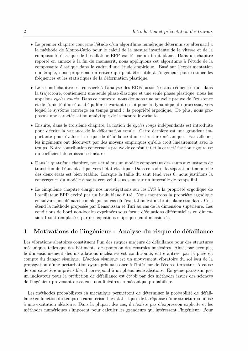
• Le premier chapitre concerne l’etude d’un algorithme numerique deterministe alternatif ala methode de Monte-Carlo pour le calcul de la mesure invariante de la vitesse et de lacomposante elastique de l’oscillateur EPP excite par un bruit blanc. Dans un chapitrereporte en annexe a la fin du manuscrit, nous appliquons cet algorithme a l’etude de lacomposante elastique dans le cadre d’une etude empirique. Base sur l’experimentationnumerique, nous proposons un critere qui peut etre utile a l’ingenieur pour estimer lesfrequences et les statistiques de la deformation plastique.
• Le second chapitre est consacre a l’analyse des EDPs associees aux sequences qui, dansla trajectoire, contiennent une seule phase elastique et une seule phase plastique; nous lesappelons cycles courts. Dans ce contexte, nous donnons une nouvelle preuve de l’existenceet de l’unicite d’un etat d’equilibre invariant en loi pour la dynamique du processus, verslequel le systeme converge en temps grand : la propriete ergodique. De plus, nous pro-posons une caracterisation analytique de la mesure invariante.
• Ensuite, dans le troisieme chapitre, la notion de cycles longs independants est introduitepour decrire la variance de la deformation totale. Cette derniere est une grandeur im-portante pour evaluer le risque de defaillance d’une structure mecanique. Par ailleurs,les ingenieurs ont decouvert par des moyens empiriques qu’elle croıt lineairement avec letemps. Notre contribution concerne la preuve de ce resultat et la caracterisation rigoureusedu coefficient de croissance lineaire.
• Dans le quatrieme chapitre, nous etudions un modele comportant des sauts aux instants detransition de l’etat plastique vers l’etat elastique. Dans ce cadre, la separation temporelledes deux etats est bien etablie. Lorsque la taille du saut tend vers 0, nous justifions laconvergence du modele a sauts vers celui sans saut sur un intervalle de temps fini.
• Le cinquieme chapitre elargit nos investigations sur les IVS a la propriete ergodique del’oscillateur EPP excite par un bruit blanc filtre. Nous montrons la propriete ergodiqueen suivant une demarche analogue au cas ou l’excitation est un bruit blanc standard. Celaetend la methode proposee par Bensoussan et Turi au cas de la dimension superieure. Lesconditions de bord non-locales exprimees sous forme d’equations differentielles en dimen-sion 1 sont remplacees par des equations elliptiques en dimension 2.
1 Motivations de l’ingenieur : Analyse du risque de defaillance
Les vibrations aleatoires constituent l’un des risques majeurs de defaillance pour des structuresmecaniques telles que des batiments, des ponts ou des centrales nucleaires. Ainsi, par exemple,le dimensionnement des installations nucleaires est conditionne, entre autres, par la prise encompte du danger sismique. L’action sismique est un mouvement vibratoire du sol issu de lapropagation d’une perturbation ayant pris naissance a l’interieur de l’ecorce terrestre. A causede son caractere imprevisible, il correspond a un phenomene aleatoire. En genie parasismique,un indicateur pour la prediction de defaillance est etabli par des methodes issues des sciencesde l’ingenieur provenant de calculs non-lineaires en mecanique probabiliste.
Les methodes probabilistes en mecanique permettent de determiner la probabilite de defail-lance en fonction du temps en caracterisant les statistiques de la reponse d’une structure soumisea une excitation aleatoire. Dans la plupart des cas, il n’existe pas d’expression explicite et lesmethodes numeriques s’imposent pour calculer les grandeurs qui interessent l’ingenieur. Pour

1. Motivations de l’ingenieur : Analyse du risque de defaillance 3
les structures composees d’un grand nombre de degres de libertes (d.d.l.), une telle caracterisa-tion necessite la realisation de calculs dynamiques temporels non-lineaires en nombre important.Cela rend la methode couteuse en temps.
Cependant, pour une classe de structures mecaniques repondant principalement sur leur pre-mier mode de vibration, l’etude peut se porter vers une modelisation elementaire de type oscil-lateur a un d.d.l. Dans ce contexte, il s’agit de modeles aussi bien simples que representatifsdu comportement elastique-plastique. Par exemple, les troncons de tuyauteries font partie desinstallations industrielles qui rentrent dans cette classe (voir Figures 1,2).
Figure 1: Vibration d’un troncon de tuyauterie : Illustration de la vibration d’un tronconde ligne de tuyauterie sur une table d’experimentation du CEA (Laboratoire d’Etudes de Me-canique SIsmique,EMSI). La structure est installee sur un plateau qui simule l’action sismique.La reponse de la structure a cette sollicitation presente une alternance entre les phases de de-formation elastique et les phases de deformation plastique. Ici, la deformation permanente semanifeste aux coudees basses de la tuyauterie.
En consequence, une importante litterature en sciences de l’ingenieur s’est developpee depuisquelques decennies sur l’etude des oscillateurs non-lineaires excites par un bruit blanc et leursapplications (voir [10, 13, 14, 15, 16, 28, 19, 24, 26, 12, 29, 30, 32, 34, 33, 35]).
4 Introduction et presentation des travaux
0 2 4 6 8 10 12−4
−3
−2
−1
0
1
2
3
Time (s)
Acc
eler
atio
n (g
)
0 1 2 3 4 5 6 7 8 9 10
−0.1
−0.05
0
0.05
0.1
0.15
Time (s)
Dis
plac
emen
t (m
)
SDOFSTEST
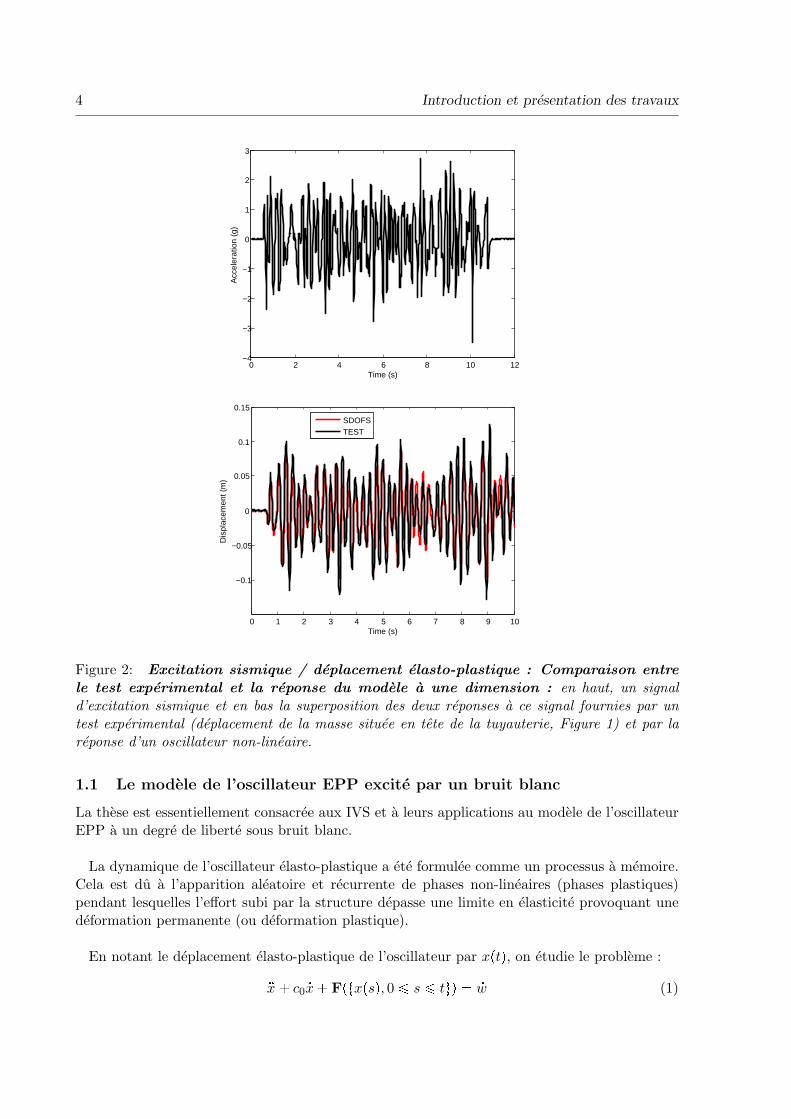
Figure 2: Excitation sismique / deplacement elasto-plastique : Comparaison entrele test experimental et la reponse du modele a une dimension : en haut, un signald’excitation sismique et en bas la superposition des deux reponses a ce signal fournies par untest experimental (deplacement de la masse situee en tete de la tuyauterie, Figure 1) et par lareponse d’un oscillateur non-lineaire.
1.1 Le modele de l’oscillateur EPP excite par un bruit blanc
La these est essentiellement consacree aux IVS et a leurs applications au modele de l’oscillateurEPP a un degre de liberte sous bruit blanc.
La dynamique de l’oscillateur elasto-plastique a ete formulee comme un processus a memoire.Cela est du a l’apparition aleatoire et recurrente de phases non-lineaires (phases plastiques)pendant lesquelles l’effort subi par la structure depasse une limite en elasticite provoquant unedeformation permanente (ou deformation plastique).
En notant le deplacement elasto-plastique de l’oscillateur par x♣tq, on etudie le probleme :
✿x� c0 ✾x� F♣tx♣sq, 0 ↕ s ↕ t✉q ✏ ✾w (1)

1. Motivations de l’ingenieur : Analyse du risque de defaillance 5
avec les conditions initiales de deplacement et de vitesse
x♣0q ✏ x , ✾x♣0q ✏ y.
Ici, c0 → 0 est un coefficient d’amortissement, w est un processus de Wiener et Ft :✏ F♣tx♣sq, 0 ↕s ↕ t✉q est une fonctionnelle non-lineaire qui depend de toute la trajectoire tx♣sq, 0 ↕ s ↕ t✉.Le processus de deformation plastique note par ∆♣tq au temps t se deduit du couple ♣x♣tq,Ftq.Nous considerons une force de type EPP
Ft ✏✩✫✪
kY si x♣tq ✏ Y �∆♣tq,k♣x♣tq ✁∆♣tqq si x♣tq Ps ✁ Y �∆♣tq, Y �∆♣tqr,
✁kY si x♣tq ✏ ✁Y �∆♣tq,(2)
ou k → 0 est un coefficient de raideur, Y est la limite elasto-plastique et ∆♣tq ✏ ´ t01t⑤Fs⑤✏kY ✉dx♣sq.
Typiquement, la force Ft alterne entre les phases elastiques ♣⑤Fs⑤ ➔ kY q et plastiques ♣⑤Fs⑤ ✏ kY q.Ainsi, D. Karnopp et T.D. Scharton [26] avaient naturellement propose une separation entre lesetats elastique et plastique. Ils ont introduit la variable ”fictive” z♣tq :✏ x♣tq✁∆♣tq et ont remar-que le simple fait qu’entre deux phases plastiques z♣tq se comporte comme un oscillateur lineaire.Ainsi, x♣tq se decompose en x♣tq ✏ z♣tq � ∆♣tq, ou on appellera z♣tq la composante elastiqueet ∆♣tq la composante plastique de x♣tq. Pendant une phase elastique, ∆♣tq reste constant et✾x♣tq ✏ ✾z♣tq. Ainsi, la variable z♣tq satisfait l’equation d’un oscillateur lineaire dont les conditionsintiales sont determinees par la phase plastique precedente :
✿z � c0 ✾z � kz ✏ ✾w. (3)
Dans ce cas, la deformation totale x♣tq est elastique puisqu’elle est portee par z♣tq. Pendant unephase plastique, la variable z♣tq reste constante (z♣tq ✏ Y ou z♣tq ✏ ✁Y ) et ✾x♣tq ✏ ✾∆♣tq. Ainsi,la vitesse de x♣tq, y♣tq :✏ ✾x♣tq est un processus d’Ornstein-Uhlenbeck et satisfait l’equation dontla condition initiale et le coefficient de derive sont determines par la vitesse a la sortie de laphase elastique precedente :
✾y � c0y ✟ kY ✏ ✾w. (4)
Dans ce cas, la deformation totale x♣tq est plastique puisqu’elle est portee par ∆♣tq. Finalement,comme les instants de transition de phase ne sont pas connus a l’avance, la resolution temporellede l’equation (1)-(2) s’obtient en considerant (3)-(4) dans le cadre de l’alternance des phaseselastique et plastique.
1.2 Le calcul du risque de defaillance et la variance de la deformation totale
Pour calculer le risque de defaillance d’une structure mecanique modelisee par un oscillateurEPP, les ingenieurs disposent de formules explicites basees sur des tests empiriques. Ces formulesreposent sur la connaissance de la variance σ2♣x♣tqq de la deformation totale. Dans le chapitre3, nous remarquerons que cette derniere a aussi le meme taux de croissance que la variancede la deformation plastique puisque x♣tq ✏ z♣tq � ∆♣tq et que z♣tq est borne. Ainsi, beaucoupde travaux en sciences de l’ingenieur ont ete consacres a l’etude de σ2♣x♣tqq. En particulier, lesingenieurs ont observe, par des tests numeriques et empiriques, que la variance de la deformationtotale croıt lineairement avec le temps (en temps grand) [11] :
limtÑ✽
σ2♣x♣tqqt
✏ σ2 (5)

6 Introduction et presentation des travaux
ou σ2 est une constante positive qui depend de Y . Pour approcher la valeur de σ2, les ingenieursont developpe des methodes heuristiques. Ces dernieres sont approximatives, mais en revanche,elles permettent d’estimer les statistiques de la deformation plastique de maniere satisfaisante.Dans la these, nous apportons une preuve mathematique de ce que les ingenieurs ont observe etnous caracterisons le coefficient σ2.
2 Une IVS modelisant l’oscillateur elasto-plastique
Les IVS ont deja ete introduites par Bensoussan et Lions [2] pour representer des diffusionsreflechies dans des domaines convexes et les inequations variationnelles aux derivees partiellesont deja ete etudiees par Duvaut et Lions [18] pour les problemes d’elasto-plasticite deterministes.Il n’est pas surprenant de voir reapparaıtre les inequations dans la modelisation des vibrationsaleatoires. Cet outil mathematique apporte le cadre exact pour etudier notamment la dynamiquede l’oscillateur EPP et ses deformations.
2.1 L’avantage de l’inequation
Les ingenieurs ont observe que l’alternance des phases reste delicate ([19, 20]). En effet, la tran-sition de l’etat plastique vers l’etat elastique est affectee par le bruit blanc. En fait, une phaseplastique debute lorsque z♣tq touche et est absorbe par Y (resp. ✁Y ) avec une vitesse positive(resp. negative) y♣tq → 0 (resp. y♣tq ➔ 0) i.e. sign♣y♣tqqz♣tq ✏ Y . Puis, elle s’arrete lorsquela vitesse change de signe. A ce moment, une phase elastique commence. Mais, la vitesse quiest affectee par le bruit blanc, change de signe une infinite de fois sur tout intervalle de temps.Souvent, cela provoque un retour rapide en phase plastique. A cause de ce phenomene, la suitedes instants de transition de phases n’est pas clairement etablie.
Alain Bensoussan et Janos Turi ont remarque que le modele utilise dans la litterature surl’oscillateur EPP est equivalent a une IVS. En effet, la relation entre la vitesse y♣tq et la com-posante elastique z♣tq est gouvernee par une inequation variationnelle :
♣dz♣tq ✁ y♣tqdtq♣φ✁ z♣tqq ➙ 0, ❅⑤φ⑤ ↕ Y, ⑤z♣tq⑤ ↕ Y.
Cette inequation a pour avantage de clarifier la dynamique sans expliciter l’alternance entre lesphases elastiques et plastiques.
2.2 Signification de la deformation plastique dans le cadre des diffusions
reflechies
L’equation (1)-(2) peut s’ecrire dans le cadre des equations differentielles stochastiques (EDS)avec un processus de reflexion. Introduisons les notations
D :✏ ♣✁✽,✽q ✂ ♣✁Y, Y q, D✁ :✏ ♣✁✽, 0q ✂ t✁Y ✉, D� :✏ ♣0,✽q ✂ tY ✉.
Les processus ♣y♣tq, z♣tqq et ∆♣tq satisfont le probleme suivant :
Probleme 1. Trouver un processus ♣y♣tq, z♣tqq a valeur dans R2 tel que
1. ♣y♣tq, z♣tqq adapte et continu,

2. Une IVS modelisant l’oscillateur elasto-plastique 7
2. il existe un processus scalaire ∆♣tq continu, a variation bornee, adapte tel que ♣y♣tq, z♣tqqverifie
dy♣tq ✏ ✁♣c0y♣tq � kz♣tqqdt� dw♣tq, z♣tq ✏ˆ t
0
y♣sqds✁∆♣tq. (6)
3. p.s. ♣y♣tq, z♣tqq P D ❨D� ❨D✁,
4. p.s.´ t2t1
1D♣y♣sq, z♣sqqd∆♣sq ✏ 0, ❅t1 ➔ t2.
admet une unique solution.
Le processus de la deformation plastique ∆♣tq joue le role du processus de reflexion. Ainsi,♣y♣tq, z♣tqq est l’unique solution de l’inequation suivante :✩✬✬✫
✬✬✪dy♣tq ✏ ✁♣c0y♣tq � kz♣tqqdt� dw♣tq,♣dz♣tq ✁ y♣tqdtq♣φ✁ z♣tqq ➙ 0,
❅⑤φ⑤ ↕ Y, ⑤z♣tq⑤ ↕ Y.
(SVI)
La justification est analogue a la preuve de [2]. Il s’agit d’une decouverte importante car elleclarifie dans un cadre mathematique solide la dynamique reelle de l’oscillateur elasto-plastique.Le processus ∆♣tq n’apparaıt pas explicitement dans l’inequation (SVI) mais il se deduit de lasolution ♣y♣tq, z♣tqq de la relation suivante
∆♣tq ✏ˆ t
0
y♣sqds✁ z♣tq.
2.3 Propriete ergodique du couple vitesse-composante elastique
A l’aide de la formule d’Ito pour les diffusions reflechies, on peut calculer le generateur infinitesi-mal Λ de ♣y♣tq, z♣tqq. Pour toute fonction ϕ suffisamment reguliere definie sur D, on a
ϕ♣y♣tq, z♣tqq ✁ ϕ♣y♣0q, z♣0qq ✁ˆ t
0
Lϕ♣y♣sq, z♣sqqds✁ˆ t
0
Rϕ♣y♣sq, z♣sqqd∆♣sq
✏ˆ t
0
∇ϕ♣y♣sq, z♣sqqdw♣sq (7)
ou les operateurs L (diffusion) et R (reflexion) s’ecrivent
Lϕ♣y, zq ✏ 1
2ϕyy ✁ ♣c0y � kzqϕy � yϕz et Rϕ♣y, zq ✏ ✁1t❇D✉♣y, zqϕz♣y, zq.
Comme ∆♣tq ✏ ´ t01tsign♣y♣sqqz♣sq✏Y ✉y♣sqds, l’egalite (7) devient :
ϕ♣y♣tq, z♣tqq ✁ ϕ♣y♣0q, z♣0qq✁ˆ t
0
✥Lϕ♣y♣sq, z♣sqq ✁ 1tsign♣y♣sqqz♣sq✏Y ✉y♣sqϕz♣y♣sq, z♣sqq
✭ds
✏ˆ t
0
ϕy♣y♣sq, z♣sqqdw♣sq.
Alors par definition du generateur, on a
Λϕ♣y0, z0q :✏ limhÑ0
1
hEtϕ♣y♣hq, z♣hqq ✁ ϕ♣y♣0q, z♣0qq⑤♣y♣0q, z♣0qq ✏ ♣y0, z0q✉

8 Introduction et presentation des travaux
satisfait
Λϕ ✏
✩✬✬✬✫✬✬✬✪
✁Aϕ♣y, zq si ♣y, zq P D,✁B�ϕ♣y, zq si ♣y, zq P D�,✁B✁ϕ♣y, zq si ♣y, zq P D✁
ou ✩✬✬✫✬✬✪
Aϕ :✏ ✁12ϕyy � ♣c0y � kzqϕy ✁ yϕz,
B�ϕ :✏ ✁12ϕyy � ♣c0y � kY qϕy,
B✁ϕ :✏ ✁12ϕyy � ♣c0y ✁ kY qϕy.
Le theoreme suivant concerne le comportement en temps long de ♣y♣tq, z♣tqq (voir [7]).
Theoreme (Bensoussan-Turi,2007). Le couple ♣y♣tq, z♣tqq est un processus de Markov ergodique.En consequence, il existe une unique mesure invariante ν vers laquelle la loi du processus con-verge. De plus, ν admet une densite de probabilite m. On notera ν♣fq l’application de la mesureinvariante sur une fonction f bornee, ainsi
ν♣fq ✏ˆ
D
f♣y, zqm♣y, zqdydz �ˆ
D�f♣y, Y qm♣y, Y qdy �
ˆ
D✁f♣y,✁Y qm♣y,✁Y qdy.
Par definition, la mesure invariante ν du processus ♣y♣tq, z♣tqq est telle que
ν♣Λϕq ✏ 0, ❅ϕ reguliere.
Pour m, cela signifie
ˆ
D
Aϕ♣y, zqm♣y, zqdydz �ˆ
D�B�ϕ♣y, Y qm♣y, Y qdy �
ˆ
D✁B✁ϕ♣y,✁Y qm♣y,✁Y qdy ✏ 0, (M)
pour toute fonction ϕ reguliere. Il s’agit de la formulation variationnelle ultra-faible de l’equationde la mesure invariante m. Le theoreme suivant concerne une caracterisation de la distributionpar dualite. (voir [8])
Theoreme (Bensoussan-Turi,2010). Pour tout λ → 0 et pour toute fonction f♣y, zq borneemesurable, il existe une solution unique uλ♣y, zq continue et bornee sur D a l’equation suivante: ✩✫
✪λuλ �Auλ ✏ f♣y, zq dans D,
λuλ �B�uλ ✏ f♣y, Y q dans D�,λuλ �B✁uλ ✏ f♣y,✁Y q dans D✁
(Pλ)
avec les conditions de bord non-locales
uλ♣y, Y q et uλ♣y,✁Y q sont continues
telle que
⑥uλ⑥✽ ↕ ⑥f⑥✽λ
et uλ est continue
et
limλÑ0
λuλ ✏ ν♣fq. (8)

3. Resultats de la these 9
3 Resultats de la these
Nous presentons maintenant en detail les chapitres de la these, nous resumons les resultatsprincipaux en les replacant dans leur contexte.
3.1 Synopsis du chapitre 1 : Analyse numerique de la mesure invariante de
l’oscillateur elastique-parfaitement-plastique excite par un bruit blanc
Dans ce chapitre, on considere un algorithme numerique deterministe pour obtenir la solutionnumerique d’un oscillateur elasto-plastique excite par un bruit blanc. Puisque les simulationsMonte-Carlo pour le processus sous-jacent sont trop lentes, une famille de solutions d’EDPsdefinissant la mesure invariante par dualite est etudiee comme alternative a la simulation prob-abiliste. Notre approche est adaptee parce que la regularite de la mesure invariante n’est passuffisante pour employer une methode des elements finis usuelle. Cette difficulte est resolue al’aide d’une methode des elements finis ultra-faible qui est developpee et mise en oeuvre avecsucces.
Pour les applications, les ingenieurs sont interesses par m, la mesure invariante du systeme,parce qu’elle decrit le regime asymptotique de l’oscillateur EPP pour les temps grands. Lasimulation numerique du systeme par une methode de Monte-Carlo est immediate a mettre enoeuvre, mais elle est lente. Dans ce chapitre, on etudie un algorithme numerique deterministealternatif a la methode de Monte-Carlo en resolvant une EDP pour m. Par ailleurs, le semi-groupe Pt associe a la solution ♣y♣tq, z♣tqq de l’inequation
dy♣tq ✏ ✁♣c0y♣tq � kz♣tqqdt� dw♣tq, ♣dz♣tq ✁ y♣tqdtq♣φ✁ z♣tqq ➙ 0, ❅⑤φ⑤ ↕ Y, ⑤z♣tq⑤ ↕ Y
avec la condition initiale ♣y♣0q, z♣0qq ✏ ♣η, ζq satisfait Pt♣fq♣η, ζq ✏ Erf♣y♣tq, z♣tqqs pour toutefonction f suffisamment reguliere. Plus precisement, on a
Erf♣y♣tq, z♣tqqs ✏ˆ
D
f♣y, zqpt♣y, zqdydz �ˆ
D�f♣y, Y qpt♣y, Y qdy �
ˆ
D✁f♣y,✁Y qpt♣y,✁Y qdy
ou pt est la densite de ♣y♣tq, z♣tqq. Ainsi, la mesure invariante m peut etre obtenue par lepassage a la limite suivant : m ✏ limtÑ✽ pt. Rappelons que cette derniere est caracterisee parune formulation variationnelle ultra-faible : pour toute fonction ϕ continue bornee
ˆ
D
m♣y, zqAϕ♣y, zqdydz �ˆ
D�m♣y, Y qB�ϕ♣y, Y qdy �
ˆ
D✁m♣y,✁Y qB✁ϕ♣y,✁Y qdy ✏ 0 (9)
ou
Aϕ :✏ ✁1
2ϕyy � ♣c0y � kzqϕy ✁ yϕz,
B�ϕ :✏ ✁1
2ϕyy � ♣c0y � kY qϕy,
B✁ϕ :✏ ✁1
2ϕyy � ♣c0y ✁ kY qϕy.
L’objectif de ce travail est de resoudre (9) et de comparer les resultats obtenus avec ceux dela methode de Monte-Carlo standard. Le point cle est la resolution d’une EDP stationnaire

10 Introduction et presentation des travaux
avec des conditions de bord non-locales et avec une fonction f suffisamment reguliere au secondmembre : ✩✫
✪λu�Au ✏ f♣y, zq dans D,
λu�B�u ✏ f♣y, Y q dans D�,λu�B✁u ✏ f♣y,✁Y q dans D✁.
(Pλ)
avec les conditions de bord non-locales
uλ♣y, Y q et uλ♣y,✁Y q sont continues.
De [8], on sait qu’il existe une solution unique uλ♣y, zq au probleme (Pλ) telle que
⑥uλ⑥✽ ↕ ⑥f⑥✽λ
et uλ est continue.
Nous justifions que cette formulation est tres importante d’un point de vue numerique puisqu’el-le permet egalement d’obtenir limtÑ✽ Erf♣y♣tq, z♣tqqs sans resoudre un probleme dependant dutemps. Nous verrons que le probleme (Pλ) est compatible avec une methode des elements finisultra-faible pour resoudre (9). Les methodes ultra-faibles ont ete utilisees theoriquement pouretablir l’existence et l’unicite de solutions a certaines classes d’EDPs mais rarement numerique-ment, excepte dans [9]. En effet, nous prouvons que
❅♣η, ζq P D, limλÑ0
λuλ♣η, ζq ✏ limtÑ✽Erf♣y♣tq, z♣tqqs
et puis que
limλÑ0
λuλ♣η, ζq ✏ˆ
D
m♣y, zqf♣y, zqdydz
�ˆ
D�m♣y, Y qf♣y, Y qdy �
ˆ
D✁m♣y,✁Y qf♣y,✁Y qdy.
Cette derniere egalite est une caracterisation equivalente de m. Cette limite ne depend pas de♣η, ζq.
3.2 Synopsis du chapitre 2 : Une approche analytique pour la theorie er-
godique des inequations variationnelles stochastiques.
Dans ce chapitre, nous presentons une nouvelle caracterisation de l’unique mesure invariante.Dans ce contexte, nous montrons une relation liant des problemes non-locaux et des problemeslocaux en introduisant la definition des cycles courts.
Cette caracterisation passe par l’etude des cycles courts definis ci-apres.
Les cycles courts
Considerons vλ♣y, zq la solution de
λvλ�Avλ ✏ f dans D, λvλ�B�vλ ✏ f dans D�, λvλ�B✁vλ ✏ f dans D✁ (10)
avec les conditions de bord vλ♣0�, Y q ✏ 0 et vλ♣0✁,✁Y q ✏ 0. C’est un probleme local. No-tons que si f est symetrique (resp. antisymetrique) alors vλ est aussi symetrique (resp. an-tisymetrique). Nous utilisons la notation vλ♣y, z; fq. Lorsque λ Ñ 0, on obtient que vλ Ñ v
ouAv ✏ f dans D, B�v ✏ f dans D�, B✁v ✏ dans D✁ (Pv)

3. Resultats de la these 11
avec les conditions de bord locales v♣0�, Y q ✏ 0 et v♣0✁,✁Y q ✏ 0. Nous utilisons la nota-tion v♣y, z; fq et on appelle v♣y, z; fq un cycle court. De plus, afin de presenter notre nouvelleformulation de la mesure invariante, nous introduisons π�♣y, zq et π✁♣y, zq telles que
Aπ� ✏ 0 dans D, π� ✏ 1 dans D�, π� ✏ 0 dans D✁ (11)
et
Aπ✁ ✏ 0 dans D, π✁ ✏ 0 dans D�, π✁ ✏ 1 dans D✁. (12)
Nous avons π� � π✁ ✏ 1, ainsi on deduit l’existence et l’unicite de solutions bornees a (11) et(12). Une nouvelle formulation de la mesure invariante est donnee par :
Theoreme 1 (Une nouvelle formulation de ν). Sous les hypotheses des theoremes precedents,la mesure invariante verifie la propriete suivante :
ν♣fq ✏ v♣0✁, Y ; fq � v♣0�,✁Y ; fq2v♣0�, Y ; 1q .
Definissons νλ♣fq :✏ vλ♣0✁,Y ;fq�vλ♣0�,✁Y ;fq2vλ♣0✁,Y ;1q , alors lorsque λÑ 0,
uλ♣y, z; fq ✁ νλ♣fqλ
Ñ u♣y, z; fq, νλ♣fq Ñ ν♣fq (13)
ou u satisfait
Au ✏ f✁ν♣fq dans D, B�u ✏ f✁ν♣fq dans D�, B✁u ✏ f✁ν♣fq dans D✁
(14)avec les conditions de bord non-locales
u♣y, Y q, et u♣y,✁Y q continues.
Enfin, nous obtenons une representation de u en relation avec les solutions de problemes locaux:
u♣y, z; fq ✏ v♣y, z; fq ✁ ν♣fqv♣y, z; 1q � π�♣y, zq ✁ π✁♣y, zq4π✁♣0✁, Y q ♣v♣0✁, Y ; fq ✁ v♣0�,✁Y ; fqq (15)
3.3 Synopsis du chapitre 3 : Comportement de la deformation plastique d’un
oscillateur EPP excite par un bruit blanc
On etudie dans ce chapitre la variance d’un oscillateur EPP excite par un bruit blanc. De nom-breux travaux en sciences de l’ingenieur, en partie experimentaux, en partie numeriques, ontmontre qu’en temps long, la variance de la deformation totale croıt lineairement avec le temps.Dans notre travail, nous demontrons ce resultat et nous caracterisons rigoureusement le coef-ficient de derive. Notre etude repose sur l’inequation variationnelle stochastique gouvernant ladynamique entre la vitesse de l’oscillateur et la force de rappel non-lineaire. Dans ce contexte,nous proposons une formulation simple et innovante de l’evolution du systeme en terme de tempsd’arret afin d’identifier des sequences independantes dans la trajectoire : les cycles longs. Nousobtenons une formule probabiliste pour le coefficient σ2. Malheureusement, cette formule nes’exprime pas sous la forme d’une EDP. Pour la calculer, il faut recourir a la simulation proba-biliste. Les resultats des simulations numeriques sont en accord avec notre prediction theorique

12 Introduction et presentation des travaux
et avec les etudes empiriques auparavant realisees par les ingenieurs.
A travers ce chapitre, nous avons pour objectif de fournir une formulation mathematiquerigoureuse (basee sur l’inequation (SVI)) des observations faites par les ingenieurs lors de leursexperimentations sur (5). Dans la suite, on introduit les cycles longs qui permettent d’etablirdes sequences independantes dans la trajectoire.
Les cycles longs
On repere les portions de trajectoires independantes de la maniere suivante : notons
τ0 :✏ inftt → 0, y♣tq ✏ 0 et ⑤z♣tq⑤ ✏ Y ✉
et s :✏ sign♣z♣τ0qq qui identifie la premiere frontiere touchee par le processus ♣y♣tq, z♣tqq. Definis-sons
θ0 :✏ inftt → τ0, y♣tq ✏ 0 et z♣tq ✏ ✁sY ✉.D’une maniere recurrente, pour n ➙ 0, connaissant θn on peut definir★
τn�1 :✏ inftt → θn, y♣tq ✏ 0 et z♣tq ✏ sY ✉θn�1 :✏ inftt → τn�1, y♣tq ✏ 0 et z♣tq ✏ ✁sY ✉.
D’apres les definitions precedentes on peut definir le n-ieme cycle long (resp. la premierepartie du cycle, la seconde partie du cycle) comme etant la portion de trajectoire delimitee parl’intervalle rτn, τn�1q, (resp. rτn, θn�1q et rθn�1, τn�1q). En effet, aux instants tτn, n ➙ 1✉ lecouple ♣y♣tq, z♣tqq est dans le meme etat qu’a l’instant τ0. Par ailleurs, il a deux types de cycleslongs selon le signe de s ✏ ✟1. L’ensemble des temps d’arret tτn, n ➙ 0✉ represente les tempsd’occurrence des cycles longs.
Comme resultat principal, nous avons obtenu le theoreme suivant :
Theoreme 2 (Caracterisation de la variance de la deformation totale en terme des cycles long).Dans le contexte precedemment defini, on a montre que
limtÑ✽
σ2♣x♣tqqt
✏E
✁´ τ1τ0y♣tqdt
✠2
E♣τ1 ✁ τ0q .
Notre preuve est basee sur la resolution d’une classe d’EDPs reliees aux cycles longs et dontles conditions de bord sont non-locales. Cette formule peut se simplifier, cela sera explique endetail.
3.4 Synopsis du chapitre 4 : Les inequations variationnelles stochastiques
comportant des sauts tendant vers 0.
L’IVS modelisant l’oscillateur EPP a pour avantage de fournir un cadre mathematique solidea la relation entre la vitesse et la force de rappel non-lineaire. Cependant, elle ne permet pas defaire la distinction explicite entre les phases elastiques et les phases plastiques. De plus, en raisondu bruit blanc, la trajectoire presente de petites et nombreuses phases elastiques (voir [19, 21]).Dans ce chapitre, nous introduisons des sauts aux instants de transition de l’etat plastique vers

3. Resultats de la these 13
l’etat elastique. Nous prouvons que la solution converge sur tout intervalle de temps fini vers lasolution du probleme sans saut, lorsque la taille du saut tend vers 0.
En terme de la dynamique de ♣y♣tq, z♣tqq, une deformation plastique commence lorsque z♣tqatteint et est absorbe par Y (resp. ✁Y ) avec une vitesse positive (resp. negative), y♣tq → 0.(resp. y♣tq ➔ 0), c’est a dire lorsque sign♣y♣tqqz♣tq ✏ Y . Ensuite, le comportement plastiquese termine lorsque la vitesse change de signe. A ce moment la, le comportement elastique estreactive. Cependant, la vitesse qui subit l’effet du bruit blanc, change de signe un nombre infinide fois sur tout intervalle de temps. Souvent, cela conduit a un retour rapide en comportementplastique, en un temps tres court. Nous appelons ce phenomene le phasage micro-elastique.Nous avons observe dans une etude empirique [21] que ce phenomene joue un role important surla frequence et les statistiques de la deformation plastique. En effet, la frequence d’occurence, lesstatistiques (duree ou valeur absolue de la deformation plastique) et la suite des temps d’entree(resp. de sortie) en phase plastique ne sont pas bien definis. Dans ce travail, nous introduisonsles IVS soumises a des sauts aux instants de transition entre les phases plastiques t⑤z♣tq⑤ ✏ Y ✉et les phases elastiques t⑤z♣tq⑤ ➔ Y ✉.
Definition du modele a sauts
Pour ǫ → 0, on introduit des sauts de taille ǫ dans la solution de l’IVS (SVI) apparaıssant dansla seconde composante z♣tq. Ainsi il est naturel de noter le nouveau processus par ♣yǫ♣tq, zǫ♣tqq.L’evolution du systeme est decrite par la procedure suivante : on commence par definir τ ǫ0 :✏ 0et ♣yǫ0♣tq, zǫ0♣tqq solution de l’IVS (SVI), avec les conditions initiales :
yǫ0♣0q ✏ y et zǫ0♣0q ✏ z,
ensuite, on definitτ ǫ1 :✏ inftt → 0, yǫ0♣tq ✏ 0 et ⑤zǫ0♣tq⑤ ✏ Y ✉.
Pour t ➙ τ ǫ1 , considerons ♣yǫ1♣tq, zǫ1♣tqq solution de l’IVS (SVI) avec les conditions initiales:
yǫ1♣τ ǫ1q ✏ 0 et zǫ1♣τ ǫ1q ✏ sign♣zǫ0♣τ ǫ1qq ♣Y ✁ ǫq ,
similairement, on definit
τ ǫ2 :✏ inftt → τ ǫ1 , yǫ1♣tq ✏ 0 et ⑤zǫ1♣tq⑤ ✏ Y ✉.
D’une maniere recurrente, connaissant τ ǫn, yǫn♣tq, et zǫn♣tq, on definit
τ ǫn�1 :✏ inftt → τ ǫn, yǫn♣tq ✏ 0 et ⑤zǫn♣tq⑤ ✏ Y ✉,
et ♣yǫn�1♣tq, zǫn�1♣tqq solution de l’IVS (SVI) avec les conditions initiales :
yǫn�1♣τ ǫn�1q ✏ 0 et zǫn�1♣τ ǫn�1q ✏ sign♣zǫn♣τ ǫn�1qq ♣Y ✁ ǫq .
On definit ensuite le processus ♣yǫ♣tq, zǫ♣tqq sur chaque intervalle de temps rτ ǫn, τ ǫn�1q de la faconsuivante :
✾yǫ♣tq ✏ ✁♣c0yǫ♣tq�kzǫ♣tqq� ✾w♣tq ; ♣ ✾zǫ♣tq✁yǫ♣tqq♣φ✁zǫ♣tqq ➙ 0 ; ❅ ⑤φ⑤ ↕ Y ; ⑤zǫ♣tq⑤ ↕ Y
(16)

14 Introduction et presentation des travaux
avec les conditions de sauts :
yǫ♣τ ǫn✁q ✏ 0, zǫ♣τ ǫn✁q ✏ zǫn✁1♣τ ǫnq,et
yǫ♣τ ǫnq ✏ 0, zǫ♣τ ǫnq ✏ sign♣zǫn✁1♣τ ǫnqq♣Y ✁ ǫq.Remarque 1. Par construction, le processus ♣yǫ♣tq, zǫ♣tqq est continu a droite et a une limite agauche (cadlag). En particulier, pour chaque temps T → 0 fixe, le nombre de sauts apparaissantdans l’intervalle ♣0, T s est fini p.s.
Nous prouvons que la solution ♣yǫ♣tq, zǫ♣tqq converge vers ♣y♣tq, z♣tqq sur tout intervalle fini,lorsque ǫ tend vers 0 au sens du resultat suivant :
Resultat de convergence
Theoreme 3. Supposons k → X�♣c0q :✏ 12
✁✁ c0
3� c0
❜19� 4 c0
6
✠. Pour T → 0, les processus
♣y♣tq, z♣tqq et ♣yǫ♣tq, zǫ♣tqq, satisfaisant (SVI) et (16) respectivement, verifient la propriete deconvergence suivante :
1
ǫE
✒sup
0↕t↕T
✦⑤y♣tq ✁ yǫ♣tq⑤2 � k ⑤z♣tq ✁ zǫ♣tq⑤2
✮✚Ñ 0 lorsque ǫÑ 0.
3.5 Synopsis du chapitre 5 : Resolution des problemes de Dirichlet degeneres
associes a la propriete ergodique d’un oscillateur elasto-plastique excite
par un bruit blanc filtre
On definit une IVS pour modeliser un oscillateur elasto-plastique excite par un bruit blanc filtre.Nous prouvons la propriete ergodique du processus sous-jacent et nous caracterisons sa mesureinvariante. On etend la methode de A.Bensoussan et J. Turi ([7]) avec une difficulte supplemen-taire due a l’accroissement de la dimension. Les conditions de bord non-locales exprimees sousforme d’equations differentielles en dimension 1 sont remplacees par des equations elliptiques endimension 2. Dans ce contexte, la methode de Khasminskii ([27]) conduit a l’etude de problemesde Dirichlet degeneres avec des conditions de bord non-locales exprimees sous forme d’EDPs.
Les oscillateurs non-lineaires soumis a des vibrations aleatoires sont des modeles simples etutiles pour predire la reponse d’une structure mecanique sollicitee au dela de sa limite en elas-ticite. Lorsque l’excitation est un bruit blanc, une importante litterature s’est constituee sur cesujet (voir [14, 15, 16, 28, 19, 20, 24, 26]). Dans le travail mentionne de A. Bensoussan et J. Turi,la reponse d’un oscillateur elasto-plastique parfait excite par un bruit blanc peut etre modeliseepar une IVS. Dans ce nouveau contexte mathematique, ils ont prouve l’existence et l’unicited’un etat d’equilibre invariant en loi pour la dynamique du processus, vers lequel le systemeconverge en temps grand : la propriete ergodique. De plus, les resultats dans [7] fournissent uncadre rigoureux pour acceder aux grandeurs qui interessent l’ingenieur ([19, 20, 26]). Cependant,pour les ingenieurs, le choix du bruit blanc n’est pas suffisamment realiste. Dans ce papier, nousproposons de considerer une excitation dans un sens qui peut etre plus realiste. Notre modelegeneralise [7] en choisissant un processus d’Ornstein-Uhlenbeck reflechi. En consequence, encomparant notre modele avec l’oscillateur EPP excite par un bruit blanc, un troisieme processusapparaıt dans l’inequation variationnelle.

3. Resultats de la these 15
Considerons w♣tq and w♣tq, deux processus de Wiener independants et x♣tq un processusd’Ornstein-Ulhenbeck reflechi
dx♣tq ✏ ✁αx♣tqdt� dw♣tq � 1tx♣tq✏✁L✉dξ1♣tq ✁ 1tx♣tq✏L✉dξ2♣tq.Ici, le processus ξ :✏ t♣ξ1♣tq, ξ2♣tqq, t ➙ 0✉ contraint x♣tq a prendre ses valeurs dans r✁L,Ls.Dans ce modele, l’excitation est donnee par
✁βx♣tqdt� dw♣tq. (17)
L’inequation variationnelle stochastique est constituee par✩✬✬✬✬✬✬✬✬✫✬✬✬✬✬✬✬✬✪
dx♣tq ✏ ✁αx♣tqdt� dw♣tq � 1tx♣tq✏✁L✉dξ1t ✁ 1tx♣tq✏L✉dξ2t ,
dy♣tq ✏ ✁♣βx♣tq � c0y♣tq � kz♣tqqdt� dw♣tq,♣dz♣tq ✁ y♣tqdtq♣ζ ✁ z♣tqq ➙ 0,
⑤ζ⑤ ↕ Y,
⑤z♣tq⑤ ↕ Y.
(18)
Si β ✘ 0, x♣tq apparaıt dans la dynamique de y♣tq. Dans ce cas nous appellerons ce modelecas 2d. Sinon β ✏ 0, x♣tq n’est plus implique dans le modele et dans ce cas, le couple ♣y♣tq, z♣tqqsatisfait le probleme de l’oscillateur EPP excite par un bruit blanc de [7], qui sera appele cas 1d.
Notation 1. Introduisons les operateurs
Au :✏ 1
2uyy � 1
2uxx ✁ αxux ✁ ♣βx� c0y � kzquy � yuz,
B�u :✏ 1
2uyy � 1
2uxx ✁ αxux ✁ ♣βx� c0y � kY quy,
B✁u :✏ 1
2uyy � 1
2uxx ✁ αxux ✁ ♣βx� c0y ✁ kY quy.
Le generateur infinitesimal Λ de ♣x♣tq, y♣tq, z♣tqq est donne par :
Λ : φ ÞÑ✧Aφ si z Ps ✁ Y, Y r,B✟φ si z ✏ ✟Y,✟y → 0.
Notation 2.
O :✏ ♣✁L,Lq✂R✂♣✁Y, Y q; O� :✏ ♣✁L,Lq✂♣0,�✽q✂tY ✉; O✁ :✏ ♣✁L,Lq✂♣✁✽, 0q✂t✁Y ✉.Notre resultat principal est le suivant :
Theoreme 4. Il existe une unique mesure de probabilite ν sur O ❨O✁ ❨O� satisfaisantˆ
O
Aφdν �ˆ
O✁B✁φdν �
ˆ
O�B�φdν ✏ 0, ❅φ reguliere.
De plus, ν a une densite de probabilite m qui satisfaitˆ
O
m♣x, y, zqdxdydz �ˆ
O�m♣x, y, Y qdxdy �
ˆ
O✁m♣x, y,✁Y qdxdy ✏ 1,
ou

16 Introduction et presentation des travaux
• tm♣x, y, zq, ♣x, y, zq P O✉ est la partie elastique,
• tm♣x, y, Y q, ♣x, yq P O�✉ est la partie plastique positive,
• et tm♣x, y,✁Y q, ♣x, yq P O✁✉ est la partie plastique negative.
De plus, m satisfait au sens des distributions l’equation suivante :
α❇❇x rxms �
❇❇y r♣βx� c0y � kzqms ✁ y
❇m❇z � 1
2
❇2m
❇x2� 1
2
❇2m
❇y2✏ 0, dans O,
et sur les bords
ym� ❇❇x rxms �
❇❇y r♣βx� c0y � kY qms � 1
2
❇2m
❇x2� 1
2
❇2m
❇y2✏ 0, dans O�,
✁ym� ❇❇x rxms �
❇❇y r♣βx� c0y ✁ kY qms � 1
2
❇2m
❇x2� 1
2
❇2m
❇y2✏ 0, dans O✁,
m ✏ 0, dans ♣✁L,Lq ✂ ♣✁✽, 0q ✂ tY ✉ ❨ ♣✁L,Lq ✂ ♣0,✽q ✂ t✁Y ✉.
La preuve est basee sur la resolution d’une suite de problemes de Dirichlet interieurs et ex-terieurs, qui sont interessants en eux-memes. On met en parallele les cas 1d et 2d, afin de faciliterla lecture. Dans le cas 1d, la variable x disparaıt (β ✏ 0), nous garderons la notation A,B�, B✁pour les operateurs definis plus haut sans la variable x.
Par ailleurs, notre etude presente un interet mathematique car elle generalise la methodeproposee par le premier auteur et J. Turi [7] au cas de la dimension superieure. Les condi-tions de bord non-locales exprimees sous la forme d’equations differentielles en dimension 1sont remplacees par des EDPs elliptiques en dimension 2. Dans le premier cas, il existe dessolutions semi-explicites, ainsi les conditions de bord non-locales se reduisent a deux nombresinconnus. Dans le second cas, les solutions des equations elliptiques sur le bord n’admettentpas d’expression explicite et dependent respectivement de deux fonctions inconnues definies sur♣✁L,Lq.
Notons que le choix de l’excitation (17) est aussi motive par deux considerations techniques :
• la premiere est d’imposer (grace aux processus ξ1 et ξ2) a x♣tq d’evoluer dans l’ensemblecompact r✁L,Ls. Ainsi, dans le cadre de notre preuve, un argument de compacite permetde montrer la propriete ergodique du triplet ♣x♣tq, y♣tq, z♣tqq. Notons que cela n’est pasgenant du point de vue des applications car si l’on choisit L suffisamment grand, alors leprocessus x♣tq est similaire a un processus d’Ornstein-Ulhenbeck.
• la deuxieme concerne la decorrelation de w♣tq et w♣tq. Dans notre demarche, basee sur lesEDPs associees au triplet ♣x♣tq, y♣tq, z♣tqq, nous evitons l’apparition de termes de deriveescroisees dans le generateur infinitesimal Λ. Il s’agit d’une simplification du cas correle quiest techniquement plus complexe.

3. Resultats de la these 17
3.6 Synopsis du chapitre-annexe 6 : Une etude empirique de la deformation
plastique
Dans ce chapitre, on s’interesse aux proprietes statistiques de la deformation plastique de l’oscil-lateur EPP excite par un bruit blanc. Notre approche repose sur l’inequation gouvernant l’evolu-tion de la vitesse et de la force de rappel non-lineaire. Dans ce travail, nous etudions le phasageelastique au moyen de la mesure invariante de l’oscillateur EPP. D’abord, nous mettons en ev-idence par les simulations probabilistes le phenomene de phases micro-elastiques (aussi petitesque nombreuses). La principale difficulte associee aux phases micro-elastiques concerne leurimpact sur des grandeurs utiles a l’ingenieur comme la frequence des deformations plastiques.En particulier, la frequence des deformations plastiques ne peut pas etre evaluee. Ensuite, nouspresentons des approximations de la loi marginale de la composante elastique z♣tq en regimeinvariant et d’une expression analogue a la formule de Rice des franchissements de seuil. Cesquantites sont solutions d’EDPs. Les resultats numeriques experimentaux sur ces equationsmontrent que la composante elastique est fortement distribuee pres du bord plastique. Finale-ment, un critere empirique qui peut etre utile a l’ingenieur est fourni afin de ne pas prendreen compte les phases micro-elastiques et ainsi evaluer d’une facon realiste les statistiques de ladeformation plastique.
Rappelons qu’une deformation plastique commence lorsque z♣tq touche et est absorbe par Y(resp. Y ) avec une vitesse positive (resp. negative) y♣tq → 0 (resp. y♣tq ➔ 0); c’est a diresign♣y♣tqqz♣tq ✏ Y . Ensuite, le comportement plastique se termine lorsque la vitesse devientnulle. A ce moment, le comportement elastique est reactive. Cependant, la vitesse, qui subitle bruit blanc, change de signe une infinite de fois pendant n’importe quel petit intervalle detemps. Souvent, cela mene a un rapide retour en phase plastique. On appelle ce phenomeneles phases micro-elastiques. Elles jouent un role important dans la frequence et les statistiquesde la deformation. A cause de ce phenomene, les frequences d’occurrence, les statistiques et lasuite des temps d’entree et de sortie en phase plastique ne sont pas bien definis.
Notre but est d’etudier les proprietes du comportement plastique pendant les intervalles detemps delimites par les instants d’entree en phase plastique et les instants de franchissement deY ✁ ǫ (resp. ✁Y � ǫ) par z♣tq avec une vitesse negative (resp. positive) pour un petit ǫ. Nousappelerons ces intervalles de temps les phases plastiques elargies.
Notre approche permet de relier rigoureusement le nombre de phases plastiques elargies aunombre de franchissements de Y ✁ ǫ a vitesse negative et de ✁Y � ǫ a vitesse positive.
Pour expliquer la procedure, considerons T → 0, notons τ ǫ0 :✏ 0 et
θǫn�1 :✏ inftt → τ ǫn, ⑤z♣tq⑤ ✏ Y ✉,τ ǫn�1 :✏ inftt → θǫn�1, ⑤z♣tq⑤ ✏ Y ✁ ǫ✉, ❅n ➙ 1. (19)
On note egalement N ǫT ✏
➦n➙0 1tτǫ
n↕T ✉ le nombre de phases plastiques elargies jusqu’au tempsT . Alors, pour toute fonction f mesurable telle que f♣y, zq ✏ 0 si sign♣yqz ✘ Y et satisfaisant
ˆ
D✁⑤f♣y,✁Y q⑤m♣y,✁Y qdy �
ˆ
D�⑤f♣y, Y q⑤m♣y, Y qdy ➔ ✽,

18 Introduction et presentation des travaux
on a
1
T
ˆ T
0
f♣y♣sq, z♣sqqds ✏ N ǫT
T✂ 1
N ǫT
NǫT➳
n✏1
ˆ τǫn
θǫn
f♣y♣sq, z♣sqqds. (20)
Par ailleurs, on peut definir separement la frequence de franchissements des seuils ✟Y ✠ ǫ avecune vitesse negative ou positive par z♣tq :
ν♣Y, ǫq :✏ limTÑ✽
N ǫT
T
et la “statistique empirique” associee a la phase plastique elargie par
∆f ♣Y, ǫq :✏ limTÑ✽
1
N ǫT
NǫT➳
n✏1
ˆ τǫn
θǫn
f♣y♣sq, z♣sqqds.
Rappelons que le comportement asymptotique a ete etudie par Bensoussan et Turi dans [7].Ils ont montre que ♣y♣tq, z♣tqq est un processus de Markov ergodique satisfaisant l’inequationvariationnelle stochastique. Ainsi, il existe une unique mesure invariante, notee m♣y, zq, etcomposee de
1. une composante elastique: tm♣y, zq, ⑤z⑤ ➔ Y ✉,2. une composante plastique positive: tm♣y, Y q, y → 0✉,3. une composante plastique negative: tm♣y,✁Y q, y ➔ 0✉.
En consequence, lorsque T tend vers l’infini, (20) devient
ˆ ✽
0
f♣y, Y qm♣y, Y qdy �ˆ 0
✁✽f♣y,✁Y qm♣y,✁Y qdy ✏ ν♣Y, ǫq∆f ♣Y, ǫq. (21)
La relation precedente est essentielle puisqu’elle etablit que le produit de ν♣Y, ǫq et ∆f ♣Y, ǫqreste constant pour toute valeur de ǫ. Cependant, dans nos simulations probabilistes, nousobservons que ν♣Y, ǫq tend vers ✽ et que ∆f ♣Y, ǫq tend vers 0. Dans ce travail, nous fournissonsun critere empirique qui peut etre utile a l’ingenieur pour calibrer ǫ. Le but est de calculer unefrequence et les statistiques de la deformation plastique qui ne prennent pas en compte les phasesmicro-elastiques. D’un point de vue empirique, nous avons observe une forte concentration dela distribution de limtÑ✽ z♣tq au voisinage des bords plastiques tz ✏ ✟Y ✉. Celle-ci presentedes points de minima qui sont identifies, on les note ✟♣Y ✁ ǫ✍q. Notre approche repose sur lesEDPs associees a la seconde marginale de tm♣y, zq, ⑤z⑤ ➔ Y ✉, qui est sÑ ´✽✁✽m♣y, sqdy. Parailleurs, les frequences moyennes de franchissements de seuils ✟♣Y ✁ǫ✍q avec une vitesse positiveou negative sont calculees avec succes a l’aide d’une formule analogue a la formule de Rice [31].Cette derniere est un outil tres utilise parmi les ingenieurs. Elle est rigoureusement etablie pourles systemes purement elastiques. Plus precisement, si l’on considere le cas : Y ✏ �✽ alorsz♣tq ✏ x♣tq et le systeme (1) est decrit par le couple ♣x♣tq, y♣tqq qui est la solution de l’EDS :
dy♣tq ✏ ✁♣c0y♣tq � kx♣tqqdt� dw♣tq, dx♣tq ✏ y♣tqdt.Le couple ♣x♣tq, y♣tqq est un processus de Markov ergodique dont la mesure invariante m estdonnee explicitement par [30] :
m♣x, yq ✏ c0❄k
πexp♣✁c0kx2q exp♣✁c0y2q.
3. Resultats de la these 19
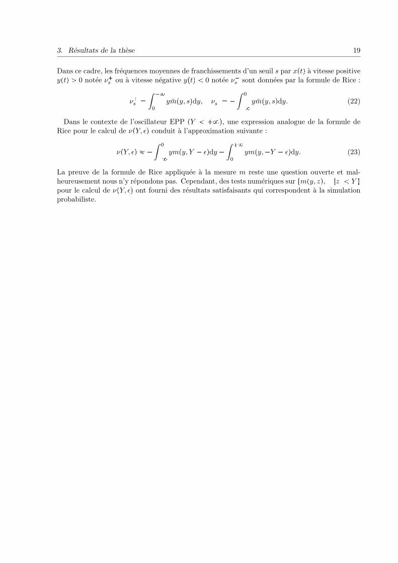
Dans ce cadre, les frequences moyennes de franchissements d’un seuil s par x♣tq a vitesse positivey♣tq → 0 notee ν�s ou a vitesse negative y♣tq ➔ 0 notee ν✁s sont donnees par la formule de Rice :
ν�s ✏ˆ �✽
0
ym♣y, sqdy, ν✁s ✏ ✁ˆ 0
✁✽ym♣y, sqdy. (22)
Dans le contexte de l’oscillateur EPP ♣Y ➔ �✽q, une expression analogue de la formule deRice pour le calcul de ν♣Y, ǫq conduit a l’approximation suivante :
ν♣Y, ǫq ✓ ✁ˆ 0
✁✽ym♣y, Y ✁ ǫqdy �
ˆ �✽
0
ym♣y,✁Y � ǫqdy. (23)
La preuve de la formule de Rice appliquee a la mesure m reste une question ouverte et mal-heureusement nous n’y repondons pas. Cependant, des tests numeriques sur tm♣y, zq, ⑤z⑤ ➔ Y ✉pour le calcul de ν♣Y, ǫq ont fourni des resultats satisfaisants qui correspondent a la simulationprobabiliste.
20 Introduction et presentation des travaux
PUBLICATIONS
1. A. Bensoussan, L. Mertz, O. Pironneau, J. Turi, An Ultra Weak Finite Element Method asan Alternative to a Monte Carlo Method for an Elasto-Plastic Problem with Noise, SIAMJ. Numer. Anal. , 47(5) (2009), 3374–3396.
2. A. Bensoussan, L. Mertz, An analytic approach to the ergodic theory of stochastic varia-tional inequalities, submitted to Comptes Rendus Acad. Sci. Paris
3. A. Bensoussan, L. Mertz Behavior of the plastic deformation of an elasto-perfectly-plasticoscillator with noise, submitted to Comptes Rendus Acad. Sci. Paris
4. A. Bensoussan, H. Jasso-Fuentes, S. Menozzi, L. Mertz Asymptotic analysis of stochasticvariational inequalities modeling an elasto-plastic problem with vanishing jumps, submittedto Asymptotic Analysis
5. A. Bensoussan, L. Mertz, Degenerate Dirichlet problems related to the ergodic theory foran elasto-plastic oscillator excited by a filtered white noise, submitted to IMA Journal ofApplied Mathematics
6. C. Feau, L. Mertz An empirical study on plastic deformations of an elasto-plastic problemwith noise, submitted to Probabilistic Engineering Mechanics
ORAL PRESENTATIONS IN INTERNATIONAL CONFERENCES
1. The 8th AIMS Conference on Dynamical Systems, Differential Equations and ApplicationsDresden , Germany, May 25 - 28, 2010 Special Session 29: Applied Analysis and Dynamicsin Engineering and Sciences An ultra weak finite element method as an alternative to aMonte Carlo for an elasto-plastic problem with noise
2. SIAM Conference on Computational Science and Engineering 2011 Reno, Nevada, Febru-ary 28-March 04 A numerical application using the invariant distribution of an elasto-plastic oscillator to compute frequency of plastic deformations
3. SIAM Conference on Control and its Applications 2011 Baltimore, Maryland, USA,July 25-27 Stochastic variational inequalities and applications to random vibrations andmechanical structures
VISITING SCHOLAR : PhD research done in collaboration with A. Bensoussan.
1. The University of Texas at Dallas: 2008, 2009, 2010 (14 months) (see [3], [4],[1])
2. The Hong Kong Polytechnic University: April 2011 (see [5], [6])

Chapter 1
Numerical analysis of the invariant
measure for an elasto-plastic
problem with noise
Ce chapitre fait l’objet d’un article publie dans SIAM Journal on Numerical Analysis, [3] encollaboration avec Alain Bensoussan, Olivier Pironneau et Janos Turi.
An efficient method for obtaining numerical solutions of an elasto-plasticoscillator with noise is considered. Since Monte-Carlo simulations for theunderlying stochastic process are too slow, as an alternative, approximatesolutions of the partial differential equation defining the invariant measureof the process are studied. The regularity of the solution of that partialdifferential equation is not sufficient to employ a ”standard” finite elementmethod. To overcome the difficulty, an ultra weak finite element method hasbeen developed and successfully implemented.
1.1 Introduction
Modeling and simulation of elasto-plastic materials under random excitation has been studiedby many authors (see e.g. [20], and the bibliography therein) providing important informationon the resistance of structures to earthquakes and also on fatigue in general. To understand theproblem the simplest is to consider a rod excited at one end by a random force and clampedat the other end. We are interested by the displacement x♣tq of the free end of the rod. Thevelocity at this end point is denoted by y♣tq, and we have ✾x♣tq ✏ y♣tq. Newton’s law implies✾y♣tq ✏ ✁♣c0y♣tq � F ♣tx♣sq, 0 ↕ s ↕ t✉q � f♣tq where ✁c0y♣tq is a damping term, ✁F ♣tx♣sq, 0 ↕s ↕ t✉q is a nonlinear restoring force and f♣tq is the force applied at the free end of the rod. Weassume that f♣tq is white noise. The conservation of forces written as a stochastic differentialequation (SDE) is
dy♣tq ✏ ✁♣c0y♣tq � F ♣tx♣sq, 0 ↕ s ↕ t✉qqdt� dw♣tq (1.1)
where w♣tq is a standard Wiener process.
21

22 Chapter 1. Numerical analysis of the invariant distribution
Beyond a given threshold ⑤F ♣tx♣sq, 0 ↕ s ↕ t✉q⑤ ✏ kY for the nonlinear restoring force thematerial goes through plastic deformation. Introducing ∆♣tq, the total plastic yielding accumu-lated up to time t, we can define a new state variable z♣tq as z♣tq ✏ x♣tq ✁ ∆♣tq. It followsthat in the plastic regime, ✾z♣tq ✏ 0, while y♣tq satisfies (1.1) where now the restoring force,F ♣tx♣sq, 0 ↕ s ↕ t✉q, is written as F ♣tX♣sq, 0 ↕ s ↕ t✉q ✏ kz♣tq for some constant k and⑤z♣tq⑤ ↕ Y . This is the nonlinear single degree of freedom model of [20]; its mechanical analogyis a system containing a linear mass, dashpot and spring and Coulomb friction-slip joint studiedin [26].
In [7] it is shown that (1.1) is equivalent to a stochastic variational inequality (SVI):
✩✬✬✫✬✬✪
dy♣tq ✏ ✁♣c0y♣tq � kz♣tqqdt� dw♣tq,♣dz♣tq ✁ y♣tqdtq♣ζ ✁ z♣tqq ➙ 0,⑤ζ⑤ ↕ Y,
⑤z♣tq⑤ ↕ Y.
(1.2)
This system is shown to be well posed for a given probability distribution ψ of the initialcondition ♣y♣0q, z♣0qq. In [7] existence, uniqueness are proven for a given probability law for♣y♣0q, z♣0qq; ergodicity is also shown. Hence, for the process ♣y♣tq, z♣tqq, there exists a uniqueinvariant distribution ν on D ❨ D� ❨ D✁ where D :✏ R ✂ ♣✁Y, Y q is the elastic domain,D� :✏ ♣0,✽q ✂ tY ✉ is the positive plastic domain and D✁ :✏ ♣✁✽, 0q ✂ t✁Y ✉ is the negativeplastic domain. The invariant distribution ν has a probability density function (pdf)m composedof three L1 functions
1. an elastic part: m♣y, zq on D,
2. a positive plastic part: m♣y, Y q on D�,
3. a negative plastic part: m♣y,✁Y q on D✁
where m♣y, zq,m♣y, Y q,m♣y,✁Y q ➙ 0 satisfy
ˆ
D
m♣y, zqdydz �ˆ
D�m♣y, Y qdy �
ˆ
D✁m♣y,✁Y qdy ✏ 1.
Moreover, the law of the process ♣y♣tq, z♣tqq converges to ν as t goes to ✽ : for all boundedmeasurable functions f ,
limtÑ✽Erf♣y♣tq, z♣tqqs ✏
ˆ
D
f♣y, zqm♣y, zqdydz�ˆ
D�f♣y, Y qm♣y, Y qdy�
ˆ
D✁f♣y,✁Y qm♣y,✁Y qdy.
For applications, engineers are interested in m because that describes the asymptotic regime forlarge times. The numerical simulation of the system by a Monte-Carlo method is straightforwardto implement but it is slow. The paper provides a deterministic numerical method, by solving apartial differential equation (PDE) for m. In addition, the semi-group Pt related to ♣y♣tq, z♣tqqsatisfies Pt♣fq♣η, ζq ✏ Erf♣y♣tq, z♣tqqs with ♣y♣0q, z♣0qq ✏ ♣η, ζq for any bounded measurablefunction f . More precisely, we have
Erf♣y♣tq, z♣tqqs ✏ˆ
D
f♣y, zqpt♣y, zqdydz �ˆ
D�f♣y, Y qpt♣y, Y qdy �
ˆ
D✁f♣y,✁Y qpt♣y,✁Y qdy.

1.1. Introduction 23
where pt is the pdf of ♣y♣tq, z♣tqq and the invariant distribution m can be obtained by m ✏limtÑ✽ pt. The latter is characterized by an ultra-weak variational formulation: for all smoothfunctions ϕ
ˆ
D
m♣y, zqAϕ♣y, zqdydz �ˆ
D�m♣y, Y qB�ϕ♣y, Y qdy �
ˆ
D✁m♣y,✁Y qB✁ϕ♣y,✁Y qdy ✏ 0 (1.3)
where
Aϕ :✏ ✁1
2ϕyy � ♣c0y � kzqϕy ✁ yϕz,
B�ϕ :✏ ✁1
2ϕyy � ♣c0y � kY qϕy,
B✁ϕ :✏ ✁1
2ϕyy � ♣c0y ✁ kY qϕy.
The purpose of the paper is to solve (1.3) and compare the results with a standard Monte-Carlosimulation. The key point is to solve a nonlocal PDE which does not depend on time with afunction f sufficiently regular at the right hand side:✩✫
✪λu�Au ✏ f♣y, zq in D,
λu�B�u ✏ f♣y, Y q in D�,λu�B✁u ✏ f♣y,✁Y q in D✁.
(Pλ)
with the nonlocal boundary conditions
uλ♣y, Y q and uλ♣y,✁Y q continuous.
From [8], we know that there exists a unique uλ♣y, zq solution of (Pλ) such that
⑥uλ⑥✽ ↕ ⑥f⑥✽λ
and uλ are continuous.
In this work, we justify that this formulation is very relevant from a numerical point of view,since it allows also to obtain limtÑ✽ Erf♣y♣tq, z♣tqqs in a way that does not require to solve atime dependent problem. We shall see that the problem (Pλ) is compatible with an ultra weakfinite element method for solving (1.3). Indeed, ergodic theory has been proven in [7] for (1.2)which implies that
❅♣η, ζq P D, limλÑ0
λuλ♣η, ζq ✏ limtÑ✽Erf♣y♣tq, z♣tqqs
and then
limλÑ0
λuλ♣η, ζq ✏ˆ
D
m♣y, zqf♣y, zqdydz
�ˆ
D�m♣y, Y qf♣y, Y qdy �
ˆ
D✁m♣y,✁Y qf♣y,✁Y qdy,
which is an equivalent characterization of m. This limit does not depend on ♣η, ζq. The paperis organized as follows:

24 Chapter 1. Numerical analysis of the invariant distribution
First, in Section 1 we provide a formal presentation of the PDE which characterize m. Then,we argue that we cannot solve this problem by a direct approach since the non-local condition´
Dm♣y, zqdydz�´
D�m♣y, Y qdy�´D✁m♣y,✁Y qdy ✏ 1 makes difficult to deal with the boundary
conditions. Consequently, we prefer to treat the dual equation (Pλ) of the invariant distribution.Indeed, we show that this class of PDEs allows to recover an equivalent characterization of mas λ goes to 0.In Section 2, we turn to the numerical solution of (Pλ) and an ultra-weak finite element methodis derived to compute the invariant distribution m.Then, in Section 3 we study a Monte-Carlo algorithm based on (1.1) which is reformulated ina mathematically more practical form with stopping times between elastic and plastic regimes.Trajectories are simulated using the Box-Muller formula and an explicit Euler time finite differ-ence scheme. The probability density for ♣y♣T q, z♣T qq P ♣y, y�dyq✂♣z, z�dzq is computed andits limit m♣y, zq when T is large is the final product of these simulations. A comparison withthe results obtained by the ultra-weak finite element method is provided. As usual in dimension2, here Monte-Carlo method is slower than finite element method.
In conclusion we remark that the ultra-weak method is certainly harder to program comparedwith Monte-Carlo algorithms but it is faster and, most importantly, more precise even though itis hampered by the necessity to choose several important parameters such as the place at whichthe computational domain is truncated.
1.2 An equivalent characterization for the invariant measure
In this section, we give a formal presentation of the equation related to m and we argue that wecannot solve it by a direct approach. Testing m with (Pλ), we obtain on D
λ
ˆ
D
uλ♣y, zqm♣y, zqdydz ✁ˆ
D
f♣y, zqm♣y, zqdydz ✏ˆ
D
✧1
2uλ,yy ✁ ♣c0y � kzquλ,y � yuλ,z
✯m♣y, zqdydz
which means
λ
ˆ
D
uλ♣y, zqm♣y, zqdydz ✁ˆ
D
f♣y, zqm♣y, zqdydz ✏ˆ
D
uλ♣y, zq✧
1
2myy � ❇
❇y r♣c0y � kzqms ✁ ym
✯dydz
�ˆ ✽
✁✽yuλ♣y, Y qm♣y, Y qdy ✁
ˆ ✽
✁✽yuλ♣y,✁Y qm♣y,✁Y qdy.
Also, we have on D�
λ
ˆ
D�uλ♣y, Y qm♣y, Y qdy ✁
ˆ
D�f♣y, Y qm♣y, Y qdy ✏
ˆ
D�uλ♣y, Y q
✧1
2myy � ❇
❇y r♣c0y � kY qms✯
dy
� uλ♣0�, Y q✧
1
2my♣0�, Y q � kY m♣0�, Y q
✯✁ 1
2uλ,y♣0�, Y qm♣0�, Y q

1.2. An equivalent characterization for the invariant measure 25
and on D✁
λ
ˆ
D✁uλ♣y,✁Y qm♣y,✁Y qdy ✁
ˆ
D✁f♣y,✁Y qm♣y,✁Y qdy ✏
ˆ
D✁uλ♣y,✁Y q
✧1
2myy � ❇
❇y r♣c0y ✁ kY qms✯
dy
� uλ♣0✁,✁Y q✧kY m♣0✁,✁Y q ✁ 1
2my♣0✁,✁Y q
✯� uλ,y♣0✁,✁Y q1
2m♣0✁,✁Y q
Finally, collecting terms we obtain
ˆ ✽
0
uλ♣y, Y q✧ym♣y, Y q � ❇
❇y r♣c0y � kY qms � 1
2myy
✯dy
�ˆ 0
✁✽uλ♣y,✁Y q
✧✁ym♣y,✁Y q � ❇
❇y r♣c0y ✁ kY qms � 1
2myy
✯dy
�ˆ 0
✁✽yuλ♣y, Y qm♣y, Y qdy ✁
ˆ ✽
0
yuλ♣y,✁Y qm♣y,✁Y qdy
�ˆ
D
uλ♣y, zq✧
1
2myy � ❇
❇y r♣c0y � kzqms ✁ ym
✯dydz
�uλ♣0�, Y q✧
1
2my♣0�, Y q � kY m♣0�, Y q
✯✁ 1
2uλ,y♣0�, Y qm♣0�, Y q
�uλ♣0✁,✁Y q✧
1
2my♣0✁,✁Y q ✁ kY m♣0✁,✁Y q
✯� 1
2uλ,y♣0✁,✁Y qm♣0✁,✁Y q
✏λ
ˆ
D
uλ♣y, zqm♣y, zqdydz ✁ˆ
D
f♣y, zqm♣y, zqdydz
�λˆ
D�uλ♣y, Y qm♣y, Y qdy ✁
ˆ
D�f♣y, Y qm♣y, Y qdy
�λˆ
D✁uλ♣y,✁Y qm♣y,✁Y qdy ✁
ˆ
D✁f♣y,✁Y qm♣y,✁Y qdy.
Now, using that we also have
❅♣η, ζq, uλ♣η, ζq Ñ ✽, λuλ♣η, ζq Ñ ν♣fq, uλ,y♣0�, Y q Ñ 0, uλ,y♣0✁,✁Y q Ñ 0,
when λ goes to 0, we deduce a formal equation for m which is the following:✩✬✬✬✬✬✬✬✬✬✫✬✬✬✬✬✬✬✬✬✪
✁ymz � ❇❇y rm♣c0y � kzqs � 1
2myy ✏ 0 in D,
⑤y⑤m� ❇❇y rm♣c0y � kzqs � 1
2myy ✏ 0 on tsign♣yqz ✏ Y ✉,m ✏ 0 on tsign♣yqz ✏ ✁Y ✉,
12my♣0�, Y q � kY m♣0�, Y q ✏ 0,
12my♣0✁,✁Y q ✁ kY m♣0✁,✁Y q ✏ 0
(1.4)
with
m ➙ 0,
ˆ
D
m♣y, zqdydz �ˆ ✽
0
m♣y, Y qdy �ˆ 0
✁✽m♣y,✁Y qdy ✏ 1.

26 Chapter 1. Numerical analysis of the invariant distribution
The last condition is essential since it express that m cannot be 0 (as a probability density func-tion). Moreover, this express a non-local condition which makes difficult to treat the functionon the boundaries. Consequently, we do not know how solve m by a direct approach.
Now, let us recover from the problem (Pλ) an equivalent characterization for the invariantdistribution as λ goes to 0.
Proposition 1. Consider uλ the solution of (Pλ), then for all ♣η, ζq P D, we have
limλÑ0
λuλ♣η, ζq ✏ˆ
D
m♣y, zqf♣y, zqdydz �ˆ
D✁m♣y,✁Y qf♣y,✁Y qdy �
ˆ
D�m♣y, Y qf♣y, Y qdy
(1.5)
Proof. The result is a direct consequence of the ergodic theory for ♣y♣tq, z♣tqq.Remark 1. The formulation (1.5) is numerically relevant because we can compute
limtÑ✽Erf♣y♣tq, z♣tqqs
in a way which does not require to solve a time dependent problem.
We shall now show how to use (1.5) to compute m.
1.2.1 Computation of m
Assume that m P L2. Next, we consider ♣giqiPI a set of independent piecewise continuousfunctions in L2♣Dq ❨ L2♣D✁q ❨ L2♣D�q and we approximate tm♣y, zq, ♣y, zq P D✉ in L2♣Dq,tm♣y, Y q, y → 0✉ in L2♣D�q, tm♣y,✁Y q, y ➔ 0✉ in L2♣D✁q, by
➦iPI mig
i where tmi, i P I✉ is asequence of real numbers. To each basis function gi,i P I, we associate the unique solution ui of(Pλ) where gi is at the right hand side. We shall build m by inverting (1.5); this means solvinga linear system with matrix
Ai,j ✏ˆ
D
gi♣y, zqgj♣y, zqdzdy �ˆ 0
✁✽gi♣y,✁Y qgj♣y,✁Y qdy �
ˆ ✽
0
gi♣y, Y qgj♣y, Y qdy (1.6)
Note that (1.5) is also ♣Amqi ✏ ♣limλÑ0 λuiq.
1.3 Numerical result with the equivalent characterization for
the invariant measure
For the computations, we need to truncate D into DL and add an artificial condition on y ✏ ✟L.We denote
D�L ✏ t0 ➔ y ➔ L, z ✏ Y ✉ and D✁L ✏ t✁L ➔ y ➔ 0, z ✏ ✁Y ✉.We add a Neumann condition on the boundary y ✏ ✟L:✩✬✬✫
✬✬✪λu�Au ✏ g in DL,
λu�B�u ✏ g� in D�L ,λu�B✁u ✏ g✁ in D✁L ,
❇nu ✏ 0 on ✁ Y ➔ z ➔ Y, y ✏ ✟L.(1.7)
We found that the choice of L is critical, it needs to be small to reduce the computing time andlarge for precision. Next, the main difficulty was to deal with boundary conditions.

1.3. Numerical result with the equivalent characterization for the invariant measure 27
1.3.1 A superposition method for the boundary conditions
We observed that the conditions at 0 ➔ y ➔ L, z ✏ ✟Y are 2 autonomous ODE in the y variablewhich could be solved separately in order to obtain non homogenous Dirichlet conditions for u.But, we needed to impose appropriate boundaries conditions at 0 and at ✟L.
It seemed reasonable to impose homogenous Neumann conditions at ♣y, zq ✏ ♣✟L,✟Y q. But,the values of u – denoted by u✟ – at y ✏ 0, z ✏ ✟Y are unknown, so we shall use the linearityof u with respect to these real numbers and dertermine them later.
Computation of u✟
In [8] it is shown that uλ is continuous, so continuity at the points ♣0, Y q and ♣0,✁Y q of uλ arethe equations which determine the unknown constants of u✟ .By linearity the solution of (1.7) is also a linear combination of the three following problems:✩✫
✪λu0 �Au0 ✏ g in D,
λu0 �B�u0 ✏ g� in D�L ,λu0 �B✁u0 ✏ g✁ in D✁L ,
with u0,� ✏ 0, u0,✁ ✏ 0,
✩✫✪
λu1 �Au1 ✏ 0 in D,
λu1 �B�u1 ✏ 0 in D�L ,λu1 �B✁u1 ✏ 0 in D✁L ,
with u1,� ✏ 1, u1,✁ ✏ 0,
✩✫✪
λu2 �Au2 ✏ 0 in D,
λu2 �B�u2 ✏ 0 in D�L ,λu2 �B✁u2 ✏ 0 in D✁L ,
with u2,� ✏ 0, u2,✁ ✏ 1.
We must find α and β such that u ✏ u0 � αu1 � βu2 is continuous in ♣0,✁Y q and ♣0, Y q, i.e.
u0♣0�, Y q � αu1♣0�, Y q � βu2♣0�, Y q ✏ u0♣0✁, Y q � αu1♣0✁, Y q � βu2♣0✁, Y qu0♣0�,✁Y q � αu1♣0�,✁Y q � βu2♣0�,✁Y q ✏ u0♣0✁,✁Y q � αu1♣0✁,✁Y q � βu2♣0✁,✁Y q
Finally, we solve the following linear system.✂u1♣0�, Y q ✁ u1♣0✁, Y q u2♣0�, Y q ✁ u2♣0✁, Y q
u1♣✁0�,✁Y q ✁ u1♣0✁,✁Y q u2♣0�,✁Y q ✁ u2♣0✁,✁Y q✡✂
α
β
✡✏✂
u0♣0✁, Y q ✁ u0♣0�, Y qu0♣0✁,✁Y q ✁ u0♣0�,✁Y q
✡
Test of Convergence of λuλ to a constant value
We have verified numerically that λuλ converges, to a constant value. Figure 1.1-1.2 correspondsto the following choice:
g♣y, zq ✏ 1
2πσzσye✁ 1
2z2
σ2z e✁ 1
2
y2
σ2y (1.8)
In figure 1.3-1.4, g is similar but non zero on D✟:
g♣y, zq ✏ 1
2πσzσye✁ 1
2
♣z✁Y q2σ2
z e✁ 1
2
y2
σ2y (1.9)

28 Chapter 1. Numerical analysis of the invariant distribution
where σz ✏ σy ✏❛
1④200. Both plots show that indeed λuλ tends to a constant when λ tendsto zero.
1.3.2 Computing m by an ultra-weak finite element method
Given a mesh of DL generated with the software freefem++, we consider a family of gaussianfunction centered on each node ♣yi, ziq of the mesh.
gi♣y, zq ✏ 1
2πσzσye✁ 1
2♣ z✁zi
σzq2e✁ 1
2♣ y✁yi
σyq2
Then we solve the problem (1.7) by a finite element method of degree one, also using freefem++.Finally we solve the linear system for m. The results are shown on figure 1.5,1.6 and thecomparison with the Monte-Carlo method is given of Figure 1.10. We denote mN the solutiongiven by the ultra weak finite element method where N is the number of basis functions.

1.3. Numerical result with the equivalent characterization for the invariant measure 29
-1-0.5
0 0.5
1 -10-5
0 5
10
0
0.5
1
1.5
2
2.5
3
"lambdaUlambda.txt"
-1-0.5
0 0.5
1 -10-5
0 5
10
0.32 0.325 0.33
0.335 0.34
0.345 0.35
0.355 0.36
0.365 0.37
"lambdaUlambda.txt"
Figure 1.1: From the top to the bottom: λuλ for λ ✏ 1.0 and λ ✏ 10✁1, with g♣y, zq ✏1
2πσzσye✁ 1
2z2
σ2z e✁ 1
2
y2
σ2y and σz ✏ σy ✏
❛1④200.

30 Chapter 1. Numerical analysis of the invariant distribution
-1-0.5
0 0.5
1 -10-5
0 5
10
0.333 0.33305 0.3331
0.33315 0.3332
0.33325 0.3333
0.33335 0.3334
0.33345 0.3335
"lambdaUlambda.txt"
-1-0.5
0 0.5
1 -10-5
0 5
10
0.329
0.33
0.331 0.332
0.333
0.334 0.335
0.336
0.337
"lambdaUlambda.txt"
Figure 1.2: From the top to the bottom: λuλ for λ ✏ 10✁4 and λ ✏ 10✁9, with g♣y, zq ✏1
2πσzσye✁ 1
2z2
σ2z e✁ 1
2
y2
σ2y and σz ✏ σy ✏
❛1④200.

1.3. Numerical result with the equivalent characterization for the invariant measure 31
-1-0.5
0 0.5
1 -10-5
0 5
10
0
0.5
1
1.5
2
2.5
"lambdaUlambda.txt"
-1-0.5
0 0.5
1 -10-5
0 5
10
0.205
0.21
0.215 0.22
0.225
0.23 0.235
0.24
0.245
"lambdaUlambda.txt"
Figure 1.3: From the top to the bottom: λuλ for λ ✏ 1.0 and λ ✏ 10✁1, with g♣y, zq ✏1
2πσzσye✁ 1
2
♣z✁Y q2σ2
z e✁ 1
2
y2
σ2y and σz ✏ σy ✏
❛1④200.

32 Chapter 1. Numerical analysis of the invariant distribution
-1-0.5
0 0.5
1 -10-5
0 5
10
0.217
0.21705
0.2171
0.21715
0.2172
0.21725
0.2173
0.21735
"lambdaUlambda.txt"
-1-0.5
0 0.5
1 -10-5
0 5
10
0.2145 0.215
0.2155 0.216
0.2165 0.217
0.2175 0.218
0.2185 0.219
0.2195
"lambdaUlambda.txt"
Figure 1.4: From the top to the bottom: λuλ for λ ✏ 10✁4 and λ ✏ 10✁9, with g♣y, zq ✏1
2πσzσye✁ 1
2
♣z✁Y q2σ2
z e✁ 1
2
y2
σ2y and σz ✏ σy ✏
❛1④200.

1.3. Numerical result with the equivalent characterization for the invariant measure 33
"m1.txt"
-1 -0.8 -0.6 -0.4 -0.2 0 0.2 0.4 0.6 0.8 1-8-6
-4-2
0 2
4 6
8
-0.05 0
0.05 0.1
0.15 0.2
0.25 0.3
0.35
"m2.txt"
-2 -1.5 -1 -0.5 0 0.5 1 1.5 2-8-6
-4-2
0 2
4 6
8
-0.05 0
0.05 0.1
0.15 0.2
0.25 0.3
0.35
Figure 1.5: mN computed by the Ultra Weak Method, from the top to the bottom we considerY ✏ 1, 2. When Y increases the plastic part decreases.

34 Chapter 1. Numerical analysis of the invariant distribution
"m3.txt"
-3-2
-1 0
1 2
3-8-6
-4-2
0 2
4 6
8
-0.05 0
0.05 0.1
0.15 0.2
0.25 0.3
0.35
"m4.txt"
-4 -3 -2 -1 0 1 2 3 4-8-6
-4-2
0 2
4 6
8
-0.05 0
0.05 0.1
0.15 0.2
0.25 0.3
0.35
Figure 1.6: mN computed by the Ultra Weak Method, from the top to the bottom we considerY ✏ 3, 4. When Y increases the plastic part decreases.

1.4. Monte-Carlo simulations 35
1.4 Monte-Carlo simulations
1.4.1 Reformulation with stopping times
We recall from [7] the stochastic differential equations governing the process ♣y♣tq, z♣tqq of (1.1)corresponding to the elastic and plastic regimes, respectively.
For n ✏ 0, 1, .. and starting with θ0 ✏ τ0 ✏ 0, we define two sets of stopping times in thefollowing way: ✧
θn�1 ✏ inftt → τn, ⑤z♣tq⑤ ✏ Y ✉τn�1 ✏ inftt → θn�1, y♣tq ✏ 0✉ (1.10)
When t P rτn, θn�1r, we have ⑤z♣tq⑤ ➔ Y and ♣y♣tq, z♣tqq satisfies:✧dy♣tq ✏ ✁♣c0y♣tq � kz♣tqqdt� dw♣tqdz♣tq ✏ y♣tqdt (1.11)
When t P rθn�1, τn�1r, we have ⑤z♣tq⑤ ✏ Y and ♣y♣tq, z♣tqq satisfies✧dy♣tq ✏ ✁♣c0y♣tq � kz♣tqqdt� dw♣tqdz♣tq ✏ 0
(1.12)
Remark 2. ♣θnqn➙1 corresponds to each entry in plastic regime. During plastic regime, whensign♣y♣tqq changes the behavior of the oscillator comes back to the elastic regime. Then ♣τnqn➙1
corresponds to each exit of plastic regime.
1.4.2 Analytic formulae
We will use later the fact that in each elastic and plastic time segments there is an analytic
formula for the solution. Let ♣y♣0q, z♣0qq ✏ ♣y, zq and let ω ✏❄
4k✁c202
. From now on, we assume4k → c20. Note that the condition 4k → c20 is needed so that ♣y♣tq, z♣tqq have real valued solutions.We have ✩✬✬✬✫
✬✬✬✪z♣tq ✏ e
✁c0t
2 tz cos ♣ωtq � 1ω♣y � c0
2zq sin ♣ωtq✉
� 1ω
´ t
0e✁
c02♣t✁sq sin ♣ω♣t✁ sqqdw♣sq,
y♣tq ✏ ✁ c02z♣tq � e✁
c0t
2 t✁ωz sin ♣ωtq � ♣y � c02zq cos ♣ωtq✉
� ´ t0e✁
c02♣t✁sq cos ♣ω♣t✁ sqqdw♣sq.
(1.13)
z♣tq is a gaussian variable with mean equal to ez♣t, z, yq and variance equal to σ2z♣tq, where
ez♣t, y, zq ✏ e✁c0t
2 tz cos ♣ωtq � 1
ω♣y � c0
2zq sin ♣ωtq✉,
σ2z♣tq ✏ 1
ω2
ˆ t
0
e✁c0s sin2 ♣ωsqds.
y♣tq is a gaussian variable with mean equal to ey♣t, y, zq and variance equal to σ2y♣tq, where
ey♣t, y, zq ✏ ✁c02ez♣t, z, yq � e✁
c0t
2 t✁ωz sin ♣ωtq � ♣y � c0
2zq cos ♣ωtq✉,
σ2y♣tq ✏
ˆ t
0
e✁c0s cos2 ♣ωsqds✁ 4c20ω2
ˆ t
0
e✁c0s sin2 ♣ωsqds✁ c0
2ω2e✁c0t sin2 ♣ωtq.

36 Chapter 1. Numerical analysis of the invariant distribution
The correlation between y♣tq and z♣tq is given by
σyz♣tq ✏ 1
2ω
ˆ t
0
e✁c0s sin ♣2ωsqds✁ c0
4ω2
ˆ t
0
e✁c0s sin2 ♣ωsqds.
When the system is in a plastic state there is an analytic solution also. Let ♣y♣0q, z♣0qq ✏ ♣y,✟Y qthen ★
z♣tq ✏ ✟Y,y♣tq ✏ ye✁c0t ✠ kY
c0♣1✁ e✁c0tq � e✁c0t❄
2c0w♣e2c0t ✁ 1q. (1.14)
1.4.3 Monte-Carlo method for computing the invariant measure
Based on these analytic solutions, a C code was written to simulate ♣y♣tq, z♣tqq. Let T → 0, N P N,and ♣tnqn✏0..N a family of time which discretize r0, T s, such that tn ✏ nδt where δt :✏ T
N.
We set Σ P M2,2♣R2q such that
ΣΣT ✏✂σ2z♣δtq σz,y♣δtq
σz,y♣δtq σ2y♣δtq
✡. (1.15)
Let ♣Gn,mqn✏0..N,m✏1,2 be random independent Gaussian N ♣0, 1q variables. Here, all gaussianrandom variables are generated by the Box-Muller formula [23] and the C function rand(). Thefinite difference scheme for (1.1) is as follows:
if ⑤z♣tnq⑤ ➔ Y , ✂z♣tn�1qy♣tn�1q
✡✏
✂ez♣δt, y♣tnq, z♣tnqqey♣δt, y♣tnq, z♣tnqq
✡� Σ
✂Gn,1Gn,2
✡, (1.16)
if ⑤z♣tnq⑤ ✏ Y ,
✂z♣tn�1qy♣tn�1q
✡✏
✄ ✟Yy♣tnqe✁c0δt ✠ kY
c0♣1✁ e✁c0δtq � e✁c0δt
❜e2c0δt✁1
2c0Gn,2
☛. (1.17)
Figure 1.7 shows a sample of trajectory of the process at T=10. Then, to compute the probabilitydensity function of ♣y♣T q, z♣T qq, we define L sufficiently large and the domains
DL :✏ ♣✁L,Lq ✂ ♣✁Y, Y q, D✁L :✏ ♣0, Lq ✂ tY ✉, D✁L :✏ ♣✁L, 0q ✂ t✁Y ✉
and the three uniform grids on DL, D�L and D✁L
G♣Ny, Nzq, G♣Nyq, G♣Nyq
for given integers Ny, Nz.The i, j-cell on DL is
Di,j ✏ ♣✁L� 2jL
Ny,✁L� 2♣j � 1qL
Nyq ✂ ♣✁Y � 2iY
Nz,✁Y � 2♣i� 1qY
Nzsq
and the j-cell on D✟L is
D�j ✏ ♣j LNy
, ♣j � 1q LNy
q, D✁j ✏ ♣✁L� jL
Ny,✁L� ♣j � 1q L
Nyq

1.4. Monte-Carlo simulations 37
-2
-1.5
-1
-0.5
0
0.5
1
1.5
2
2.5
3
3.5
-1.5 -1 -0.5 0 0.5 1 1.5
’trajectory.txt’
Figure 1.7: Example of trajectory ♣y♣tq, z♣tqqtPr0,T s, T ✏ 10.
for given 0 ↕ i ➔ Nz, 0 ↕ j ➔ Ny. Let us generate numerically N trajectories up to time Tand count the number ni,j , n
�j and n✁j of trajectories ending in Di,j ,D
�j and D✁
j . By the law of
large numbers we can approximate the probability that ♣♣y♣T q, z♣T qq P Di,jq by XNi,j :✏ ni,j
Nand
the probability that ♣♣y♣T q, z♣T qq P Dj✟q by X✟,Nj :✏ n✟j
N. By the central limit theorem we also
know the error: for instance at 5 % error
P♣♣y♣T q, z♣T qq P Di,jq P✄XNi,j ✁
1.96XNi,j♣1✁ XN
i,jq❄N
, XNi,j �
1.96XNi,j♣1✁ XN
i,jq❄N
☛
and also
P♣♣y♣T q, z♣T qq P D✟j q P
✄X✟,Nj ✁ 1.96X✟,N
j ♣1✁ X✟,Nj q❄
N, X
✟,Nj � 1.96X✟,N
j ♣1✁ X✟,Nj q❄
N
☛
The invariant measure m of the process is computed as the asymptotic limit for large T ofXNi,j and X
✟,Nj . In figure 1.8-1.9 m is shown for different values of Y , Y ✏ 1, 2, 3, 4, with
L ✏ 7, T ✏ 10, N ✏ 107. Moreover, for each Y , we can estimate the plastic part denoted bypMCY ,
pMCY :✏ P
�♣y♣T q, z♣T qq P ♣0,�✽q✟✂ tY ✉ � P�♣y♣T q, z♣T qq P ♣✁✽, 0q ✂ t✁Y ✉✟
i.e.
pMCY ✏
ˆ ✽
0
m♣y, Y qdy �ˆ 0
✁✽m♣y,✁Y qdy

38 Chapter 1. Numerical analysis of the invariant distribution
"m1M C .txt"
-1-0 .8
-0 .6-0 .4
-0 .2 0
0 .2 0 .4
0 .6 0 .8
1 -8
-6
-4
-2
0
2
4
6
8
0
0 .05
0 .1
0 .15
0 .2
0 .25
0 .3
0 .35
0 .4
"m2M C .txt"
-2-1 .5
-1-0 .5
0 0 .5
1 1 .5
2 -8
-6
-4
-2
0
2
4
6
8
0
0 .05
0 .1
0 .15
0 .2
0 .25
0 .3
Figure 1.8: Plots of mMC computed by the Monte-Carlo Method; from the top to the bot-tom we consider Y ✏ 1, 2. When Y increases the plastic part decreases, indeed pMC
1 ✏84.9r84.7,85.0s%, pMC
2 ✏ 9.62r9.61,9.63s%
and the confidence interval for a 5 % error. We denote mMC the solution given by the Monte-

1.4. Monte-Carlo simulations 39
"m3M C .txt"
-3-2
-1 0
1 2
3 -8
-6
-4
-2
0
2
4
6
8
0
0 .05
0 .1
0 .15
0 .2
0 .25
0 .3
0 .35
"m4M C .txt"
-4-3
-2-1
0 1
2 3
4 -8
-6
-4
-2
0
2
4
6
8
0
0 .05
0 .1
0 .15
0 .2
0 .25
0 .3
0 .35
Figure 1.9: Plots of mMC computed by the Monte-Carlo Method; from the top to the bot-tom we consider Y ✏ 3, 4. When Y increases the plastic part decreases, indeed pMC
3 ✏0.04764r0.04760,0.04768s%, pMC
4 ✏ 0.0 %.
Carlo method.

40 Chapter 1. Numerical analysis of the invariant distribution
0
0 .5
1
1 .5
2
2 .5
3
3 .5
4
10 20 30 40 50 60 70 80
"casY 1/erreurL2U F.txt"
"casY 2/erreurL2U F.txt"
"casY 3/erreurL2U F.txt"
"casY 4/erreurL2U F.txt"
-3 .5
-3
-2 .5
-2
-1 .5
-1
-0 .5
0
0 .5
1
1 .5
2 2 .5 3 3 .5 4 4 .5 5
"casY 1/erreurL2U Flog.txt""casY 2/erreurL2U Flog.txt""casY 3/erreurL2U Flog.txt""casY 4/erreurL2U Flog.txt"
Figure 1.10: Top: L2-Relative error :⑥mMC✁mN ⑥
L2
⑥mMC⑥L2between the result given by the Monte-Carlo
method and the results given by the Ultra Weak method, versus❄N , where N is the number of
basis functions. Bottom: The same plot in log-log scale.

1.5. Conclusion 41
1.5 Conclusion
In this work, we compared a deterministic method to a Monte-Carlo computation to computethe stationnary state of the process ♣y♣tq, z♣tqq when t Ñ ✽. The Monte-Carlo method isstraightforward but expensive. The probability density of limtÑ✽♣y♣tq, z♣tqq is also characterizedby a PDE. As we saw, classical methods, on this PDE do not work because m belong to L2 butnot to H1. So, an Ultra Weak method has been proposed to compute m. The main idea is tosolve the dual problem of m on each function of a basis of L2. Comparing the result between thetwo methods, we found less than 3 % of L2 relative difference. This deterministic method is alsoexpensive but it is more precise than the Monte-Carlo method at equal computing time so it isfaster at comparable precisions. In the future, we shall extend this approach to multidimensionalproblems, more relevant to application for earthquake engineering.
1.6 Appendix: A numerical study of elastic phasing
Let us exhibit the phenomenon of micro-elastic phases which are also small as well as numerous.
1.6.1 Direct numerical simulations
Figure 1.11 shows (a) the sojourns in the elastic and plastic phases, (b) the sojourns in micro-elastic and micro-plastic phases.
1.6.2 Approximation of the second marginal of m
In this subsection, we consider the numerical resolution of problem (Pλ). Concentration ofmicro-elastic phasing must appear in temporal averaging of ♣y♣tq, z♣tqq on long time period. Werecall that ergodicity implies
limTÑ✽
1
T
ˆ T
0
f♣y♣sq, z♣sqqds ✏ˆ
D✁m♣y,✁Y qf♣y,✁Y qdy �
ˆ
D�m♣y, Y qf♣y, Y qdy
�ˆ
D
m♣y, zqf♣y, zqdydz,
for all bounded continuous function ❅f . Consequently, m has to be affected by this phenomenon.So, we are interested in computing the second marginal of m in elastic phase that is
U : sш �✽
✁✽m♣y, sqdy, s P ♣✁Y, Y q.
For this purpose, we introduce
• Un♣sq to approximate U♣sq,
Un♣sq :✏ˆ �✽
✁✽
ˆ Y
✁Ym♣y, zqχn♣z ✁ sqdzdy.
• Wn♣sq (the derivative of Un♣sq) to compute sensibility to the threshold U ✶♣sq.
Wn♣sq :✏ n
ˆ �✽
✁✽
ˆ Y
✁Ym♣y, zq♣z ✁ sqχn♣z ✁ sqdzdy,
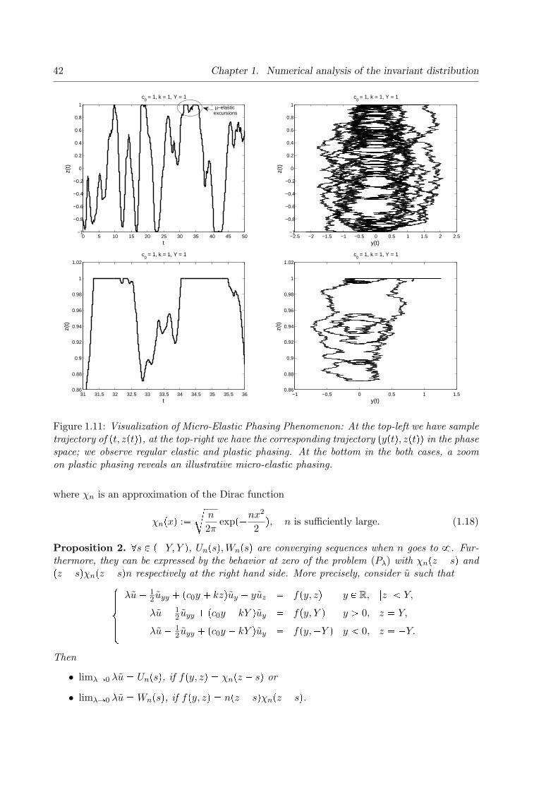
42 Chapter 1. Numerical analysis of the invariant distribution
0 5 10 15 20 25 30 35 40 45 50−1
−0.8
−0.6
−0.4
−0.2
0
0.2
0.4
0.6
0.8
1
c0 = 1, k = 1, Y = 1
z(t)
t
µ−elastic excursions
−2.5 −2 −1.5 −1 −0.5 0 0.5 1 1.5 2 2.5−1
−0.8
−0.6
−0.4
−0.2
0
0.2
0.4
0.6
0.8
1
c0 = 1, k = 1, Y = 1
z(t)
y(t)
31 31.5 32 32.5 33 33.5 34 34.5 35 35.5 360.86
0.88
0.9
0.92
0.94
0.96
0.98
1
1.02
c0 = 1, k = 1, Y = 1
z(t)
t−1 −0.5 0 0.5 1 1.5
0.86
0.88
0.9
0.92
0.94
0.96
0.98
1
1.02
c0 = 1, k = 1, Y = 1
z(t)
y(t)
Figure 1.11: Visualization of Micro-Elastic Phasing Phenomenon: At the top-left we have sampletrajectory of ♣t, z♣tqq, at the top-right we have the corresponding trajectory ♣y♣tq, z♣tqq in the phasespace; we observe regular elastic and plastic phasing. At the bottom in the both cases, a zoomon plastic phasing reveals an illustrative micro-elastic phasing.
where χn is an approximation of the Dirac function
χn♣xq :✏❝
n
2πexp♣✁nx
2
2q, n is sufficiently large. (1.18)
Proposition 2. ❅s P ♣✁Y, Y q, Un♣sq,Wn♣sq are converging sequences when n goes to ✽. Fur-thermore, they can be expressed by the behavior at zero of the problem (Pλ) with χn♣z ✁ sq and♣z ✁ sqχn♣z ✁ sqn respectively at the right hand side. More precisely, consider u such that✩✬✬✬✫
✬✬✬✪λu✁ 1
2uyy � ♣c0y � kzquy ✁ yuz ✏ f♣y, zq y P R, ⑤z⑤ ➔ Y,
λu✁ 12uyy � ♣c0y � kY quy ✏ f♣y, Y q y → 0, z ✏ Y,
λu✁ 12uyy � ♣c0y ✁ kY quy ✏ f♣y,✁Y q y ➔ 0, z ✏ ✁Y.
Then
• limλÑ0 λu ✏ Un♣sq, if f♣y, zq ✏ χn♣z ✁ sq or
• limλÑ0 λu ✏Wn♣sq, if f♣y, zq ✏ n♣z ✁ sqχn♣z ✁ sq.

1.6. Appendix: A numerical study of elastic phasing 43
Proof. As m is assumed sufficiently regular inside D, we deduce convergence of the sequences ofDirac’s approximation Un♣sq Ñ U♣sq and Wn♣sq Ñ U ✶♣sq as nÑ✽.
Computational results on the invariant distribution
In Figure 1.12, 1.13 and 1.14 (left) computations of pdf of z show up a significant concentration oflimtÑ✽ z♣tq in the neighborhood of plastic boundaries. So, in Figures 1.12,1.13 and 1.14 (right)points of inflection of U ✶ are located. For applications, we believe that we located thresholdss✟ sufficiently far away from the boundary. Indeed, note that s✟ are near but not on theboundary, thereby justifying existence of micro-elastic phasing. This phenomenon is also presentin the probabilistic numerical simulation of Un (not shown here) but it is quantified much moreaccurately with the PDEs related to the invariant distribution.
−1 −0.8 −0.6 −0.4 −0.2 0 0.2 0.4 0.6 0.8 1
0.35
0.4
0.45
0.5
0.55
0.6
0.65
s
Un(s
)
c0 = 1, k = 1, Y = 1, n = 8e3
−1 −0.8 −0.6 −0.4 −0.2 0 0.2 0.4 0.6 0.8 1−2
−1.5
−1
−0.5
0
0.5
1
1.5
2
c0 = 1, k = 1, Y = 1, n = 8e3
s
Wn(s
)
s+
s−
Figure 1.12: Un♣sq,Wn♣sq, s P ♣✁Y, Y q and location of s✟, Y ✏ 1.
−1.5 −1 −0.5 0 0.5 1 1.50
0.1
0.2
0.3
0.4
0.5
0.6
0.7
s
Un(s
)
c0 = 1, k = 1, Y = 1.5, n = 8e3
−1.5 −1 −0.5 0 0.5 1 1.5−2
−1.5
−1
−0.5
0
0.5
1
1.5
2
c0 = 1, k = 1, Y = 1.5, n = 8e3
s
Wn(s
)
s+
s−
Figure 1.13: Un♣sq,Wn♣sq, s P ♣✁Y, Y q and location of s✟, Y ✏ 1.5.

44 Chapter 1. Numerical analysis of the invariant distribution
−2 −1.5 −1 −0.5 0 0.5 1 1.5 20
0.1
0.2
0.3
0.4
0.5
0.6
0.7
s
Un(s
)
c0 = 1, k = 1, Y = 2, n = 5e3
−2 −1.5 −1 −0.5 0 0.5 1 1.5 2−1
−0.8
−0.6
−0.4
−0.2
0
0.2
0.4
0.6
0.8
1
c0 = 1, k = 1, Y = 2, n = 5e3
s
Wn(s
)
s+
s−
Figure 1.14: Un♣sq,Wn♣sq, s P ♣✁Y, Y q and location of s✟, Y ✏ 2.

Chapter 2
An analytic approach to the ergodic
theory of stochastic variational
inequalities
Ce chapitre fait l’objet d’une note soumise au Comptes Rendus Acad. Sci. Paris [5] en collabo-ration avec Alain Bensoussan.
In an earlier work made by the first author with J. Turi (Degenerate Dirich-let Problems Related to the Invariant Measure of Elasto-Plastic Oscillators,AMO, 2008), the solution of a stochastic variational inequality modeling anelasto-perfectly-plastic oscillator has been studied. The existence and unique-ness of an invariant measure have been proven. Nonlocal problems have beenintroduced in this context. In this work, we present a new characterizationof the invariant measure. The key finding is the connection between nonlo-cal PDEs and local PDEs which can be interpreted with short cycles of theMarkov process solution of the stochastic variational inequality.
Resume
Une approche analytique de la theorie ergodique des inequationsvariationnelles stochastiques. Dans un travail precedent du premier au-teur en collaboration avec Janos Turi (Degenerate Dirichlet Problems Relatedto the Invariant Measure of Elasto-Plastic Oscillators, AMO, 2008), la solu-tion d’une inequation variationnelle stochastique modelisant un oscillateurelastique-parfaitement-plastique a ete etudiee. L’existence et l’unicite d’unemesure invariante ont ete prouvees. Des problemes nonlocaux ont ete intro-duits dans ce contexte. La conclusion importante est la connexion entre desEDPs nonlocales et des EDPs locales qui peuvent etre interpretees comme lescycles courts du processus de Markov solution de l’inequation variationnellestochastique.
45

46 Chapter 2. An analytic approach of the ergodic theory of SVI
Version francaise abregee
La dynamique de l’oscillateur elastique-parfaitement-plastique s’exprime a l’aide d’une equationa memoire (voir (2.1)-(2.2)). A. Bensoussan et J. Turi ont montre que la relation entre la vitesseet la composante elastique de l’oscillateur est un processus de Markov ergodique qui satisfaitune inequation variationnelle stochastique (voir (2.3)). La solution admet une mesure invariantecaracterisee par dualite a l’aide d’une equation aux derivees partielles avec des conditions de bordnon-locales (voir (2.4)). Dans ce travail, une nouvelle preuve de la theorie ergodique est presenteeainsi qu’une nouvelle caracterisation de l’unique distribution invariante. Dans ce contexte, nousdeduisons des nouvelles formules reliant des equations aux derivees partielles avec des conditionsde bord non-locales a des problemes locaux (voir (2.10)).
2.1 Introduction
In the engineering literature, the dynamics of the elastic-perfectly-plastic (EPP) oscillator hasbeen formulated as a process x♣tq which stands for the displacement of the oscillator, evolvingwith hysteresis. The evolution is defined by the problem
✿x� c0 ✾x� F♣x♣sq, 0 ↕ s ↕ tq ✏ ✾w (2.1)
with initial conditions of displacement and velocity x♣0q ✏ x, ✾x♣0q ✏ y. Here c0 → 0 is theviscous damping coefficient, k → 0 the stiffness, w is a Wiener process; F♣x♣sq, 0 ↕ s ↕ tq is anonlinear functional which depends on the entire trajectory tx♣sq, 0 ↕ s ↕ t✉ up to time t. Theplastic deformation denoted by ∆♣tq at time t can be recovered from the pair ♣x♣tq,F♣x♣sq, 0 ↕s ↕ tqq by the following relationship:
F♣x♣sq, 0 ↕ s ↕ tq ✏✩✫✪
kY if x♣tq ✏ Y �∆♣tq,k♣x♣tq ✁∆♣tqq if x♣tq Ps ✁ Y �∆♣tq, Y �∆♣tqr,
✁kY if x♣tq ✏ ✁Y �∆♣tq.(2.2)
where Y is an elasto-plastic bound. Such elasto-plastic oscillator is simple and representative ofthe elasto-plastic behavior of a class of structure dominated by their first mode of vibration, theyare employed to estimate prediction of failure of mechanical structures. Karnopp & Scharton[26] proposed a separation between elastic states and plastic states and introduced a fictitiousvariable z♣tq :✏ x♣tq ✁∆♣tq.
Recently, the right mathematical framework of stochastic variational inequalities (SVI) mod-eling an EPP oscillator with noise has been introduced by one of the authors in [7]. AlthoughSVI have been already studied in [2] to represent reflection-diffusion processes in convex sets, noconnection with random vibration had been made so far. The inequality governs the relationshipbetween the velocity y♣tq and the variable z♣tq:
dy♣tq ✏ ✁♣c0y♣tq � kz♣tqqdt� dw♣tq, ♣dz♣tq ✁ y♣tqdtq♣φ✁ z♣tqq ➙ 0, ❅⑤φ⑤ ↕ Y, ⑤z♣tq⑤ ↕ Y.
(2.3)Let us introduce some notations.
Notation 3. D :✏ R ✂ ♣✁Y,�Y q, D� :✏ ♣0,✽q ✂ tY ✉, D✁ :✏ ♣✁✽, 0q ✂ t✁Y ✉, and thedifferential operators Aζ :✏ ✁1
2ζyy�♣c0y�kzqζy✁yζz, B�ζ :✏ ✁1
2ζyy�♣c0y�kY qζy, B✁ζ :✏
✁12ζyy � ♣c0y ✁ kY qζy. where ζ is a regular function on D.

2.1. Introduction 47
In [7], it has been shown that the probability distribution of ♣y♣tq, z♣tqq converges to an asymp-totic probability measure on D ❨D� ❨D✁ namely ν. Moreover, ν is the unique invariant dis-tribution of ♣y♣tq, z♣tqq. In addition, from [8] we know also that there exists a unique solutionuλ to the following partial differential equation (PDE)
λuλ �Auλ ✏ f in D, λuλ �B�uλ ✏ f in D�, λuλ �B✁uλ ✏ f in D✁ (2.4)
with the nonlocal boundary conditions given by the fact that uλ♣y, Y q and uλ♣y,✁Y q are con-tinuous, where λ → 0 and f is a bounded measurable function. The function uλ satisfies⑥uλ⑥✽ ↕ ⑥f⑥✽
λ, uλ is continuous and for all ♣η, ζq P D, we have limλÑ0 λuλ♣η, ζq ✏ ν♣fq. We use
the notation uλ♣y, z; fq.
Now, we introduce the short cycles to provide a new proof of the ergodic theory for (2.3). Inthis context, we derive new formulas linking PDEs with nonlocal boundary conditions to localproblems.
2.1.1 Short cycles
Let λ → 0, consider vλ♣y, zq the solution of
λvλ �Avλ ✏ f in D, λvλ �B�vλ ✏ f in D�, λvλ �B✁vλ ✏ f in D✁ (2.5)
with the local boundary conditions vλ♣0�, Y q ✏ 0 and vλ♣0✁,✁Y q ✏ 0. Also, if f is symmet-ric (resp. antisymmetric) then vλ is symmetric (resp. antisymmetric). We use the notationvλ♣y, z; fq. As λÑ 0, vλ Ñ v with
Av ✏ f in D, B�v ✏ f in D�, B✁v ✏ f in D✁ (Pv)
with the local boundary conditions v♣0�, Y q ✏ 0 and v♣0✁,✁Y q ✏ 0. We use the notationv♣y, z; fq. We call v♣y, z; fq a short cycle. We detail the solution of (Pv) in the next section. Weintroduce next π�♣y, zq and π✁♣y, zq such that
Aπ� ✏ 0 in D, π� ✏ 1 in D�, π� ✏ 0 in D✁ (2.6)
and
Aπ✁ ✏ 0 in D, π✁ ✏ 0 in D�, π✁ ✏ 1 in D✁. (2.7)
We have π� � π✁ ✏ 1, so the existence and uniqueness of a bounded solution to (2.6) and (2.7)are clear. A new formulation of the invariant distribution is given by the following theorem.
Theorem 2.1.1 (New formulation of the invariant distribution ν). Let f be a bounded measur-able function on D, we have the following analytical characterization of the invariant distribution:
ν♣fq ✏ v♣0✁, Y ; fq � v♣0�,✁Y ; fq2v♣0�, Y ; 1q .
Denote νλ♣fq :✏ vλ♣0✁,Y ;fq�vλ♣0�,✁Y ;fq2vλ♣0✁,Y ;1q . As λÑ 0,
uλ♣y, z; fq ✁ νλ♣fqλ
Ñ u♣y, z; fq, νλ♣fq Ñ ν♣fq (2.8)

48 Chapter 2. An analytic approach of the ergodic theory of SVI
where u satisfies
Au ✏ f ✁ ν♣fq in D, B�u ✏ f ✁ ν♣fq in D�, B✁u ✏ f ✁ ν♣fq in D✁
(2.9)with the nonlocal boundary conditions given by the fact that
u♣y, Y q and u♣y,✁Y q are continuous.
Then, we obtain also the representation formula
u♣y, z; fq ✏ v♣y, z; fq ✁ ν♣fqv♣y, z; 1q � π�♣y, zq ✁ π✁♣y, zq4π✁♣0✁, Y q ♣v♣0✁, Y ; fq ✁ v♣0�,✁Y ; fqq (2.10)
2.2 Analysis of the short cycles
We describe the solution of (Pv). We can write v♣y, z; fq ✏ ve♣y, z; fq � v�♣y, z; fq � v✁♣y, z; fqwith ve, v
�, v✁ satisfying
Ave ✏ f♣y, zq in D, ve ✏ 0 in D�, ve ✏ 0 in D✁, (2.11)
Av� ✏ 0 in D, v�♣y, Y q ✏ ϕ�♣y; fq in D�, v� ✏ 0 in D✁, (2.12)
andAv✁ ✏ 0 in D, v✁ ✏ 0 in D�, v✁♣y,✁Y q ✏ ϕ✁♣y; fq in D✁. (2.13)
where ϕ�♣y; fq and ϕ✁♣y; fq are defined by
✁1
2ϕ�yy � ♣c0y � kY qϕ�y ✏ f♣y, Y q, y → 0, ϕ�♣0�; fq ✏ 0 (2.14)
and
✁1
2ϕ✁yy � ♣c0y ✁ kY qϕ✁y ✏ f♣y,✁Y q, y ➔ 0, ϕ✁♣0✁; fq ✏ 0. (2.15)
We check easily the formula ϕ�♣y; fq ✏ 2´✽0dξ exp♣✁♣c0ξ2�2kY ξqq ´ ξ�y
ξf♣ζ;Y q exp♣✁2c0ξ♣ζ✁
ξqqdζ, if y ➙ 0 and also ϕ✁♣y; fq ✏ 2´✽0dξ exp♣✁♣c0ξ2 ✁ 2kY ξqq ´ ✁ξ
y✁ξ f♣ζ;✁Y q exp♣✁2c0ξ♣ζ ✁ξqqdζ, if y ↕ 0.
2.2.1 Solution to Problem (2.11)
The proof will be based on solving a sequence of Interior Exterior Dirichlet problems and a fixedpoint argument. Thus, we need to state the two following lemmas as preliminary results. It issufficient to consider f ✏ 1, with no loss of generality.
Interior Dirichlet problem
We begin with the interior problem, letD1 :✏ ♣✁y1, y1q✂♣✁Y, Y q, D�1 :✏ r0, y1q✂tY ✉, D✁1 :✏♣✁y1, 0s ✂ t✁Y ✉. Let us consider the space C�1 of continuous functions on r✁Y, Y s which are 0on Y and the space C✁1 of continuous functions on r✁Y, Y s which are 0 on ✁Y . Let ϕ� P C�1and ϕ✁ P C✁1 . We consider the problem
✁1
2ζyy � ♣c0y � kzqζy ✁ yζz ✏ 1 in D1, ζ♣y, Y q ✏ 0 in D�1 , ζ♣y,✁Y q ✏ 0 in D✁1
(2.16)with ζ♣y1, zq ✏ ϕ�♣zq and ζ♣✁y1, zq ✏ ϕ✁♣zq, if ✁Y ➔ z ➔ Y.

2.2. Analysis of the short cycles 49
Lemma 1. There exists a unique bounded solution to the equation (2.16).
Proof. It is sufficient to prove an a priori bound. For that we can assume ϕ�, ϕ✁ ✏ 0. Con-sider λ → 0 and the function θ♣y, zq ✏ exp♣λc0♣y2 � kz2qq then ✁1
2θyy � ♣c0y � kzqθy ✁ yθz ✏
θ�✁λc0 � 2λc20y
2♣1✁ λq✟. Set next H :✏ ✁♣θ � ζq then
✁1
2Hyy � ♣c0y � kzqHy ✁ yHz ✏ ✁1� θ
�λc0 ✁ 2λc20y
2♣1✁ λq✟ . (2.17)
If we pick λ → max♣1, 1c0q the right hand side of (2.17) is positive. Therefore the minimum of H
can occur only on the boundary y ✏ y1 and z ✏ Y with y → 0 or z ✏ ✁Y with y ➔ 0. It followsthat H♣y, zq ➙ ✁ exp♣λc0♣y2
1 � Y 2qq and thus also 0 ↕ ζ ↕ exp♣λc0♣y21 � Y 2qq.
Exterior Dirichlet problems
Now, we proceed by considering two exterior Dirichlet problems. Let 0 ➔ y ➔ y1, we defineDy➔y :✏ ty → y, ✁Y ➔ z ➔ Y ✉, D�y➔y :✏ ty → y, z ✏ Y ✉ and Dy➔✁y :✏ ty ➔ ✁y, ✁Y ➔z ➔ Y ✉, D✁y➔✁y :✏ ty ➔ ✁y, z ✏ ✁Y ✉ and consider
✁1
2η�yy � ♣c0y � kzqη�y ✁ yη�z ✏ 1 in Dy➔y, η�♣y, Y q ✏ 0 in D�y➔y (2.18)
with the condition η�♣y, zq ✏ ζ♣y, zq if ✁Y ➔ z ➔ Y , and
✁1
2η✁yy � ♣c0y � kzqη✁y ✁ yη✁z ✏ 1 in Dy➔✁y, η✁♣y,✁Y q ✏ 0 in D✁y➔✁y (2.19)
with the condition η✁♣✁y, zq ✏ ζ♣✁y, zq, if ✁Y ➔ z ➔ Y . We use the same notation η♣y, zq forthe two problems (2.18),(2.19) for the convenience of the reader. We have
Lemma 2. For any y → 0 there exists a unique bounded solution of (2.18),(2.19).
Proof. It is sufficient to prove the bound, we claim that ⑥ζ⑥✽ ↕ η♣y, zq ↕ ⑥ζ⑥✽� Y✁zy
, for y → y
and ⑥ζ⑥✽ ↕ η♣y, zq ↕ ⑥ζ⑥✽ � Y�zy
, for y ➔ ✁y. Consider for instance ρ♣zq ✏ ⑥ζ⑥✽ � Y✁zy
for
y → y,✁Y ➔ z ➔ Y then ✁12ρyy � ρy♣c0y � kzq ✁ yρz ✏ y
y→ 1, ρ♣y, zq ✏ ⑥ζ⑥L✽ � Y✁z
y→ ζ♣y, zq,
ρ♣y, zq ✏ ⑥ζ⑥L✽ → 0. So clearly η♣y, zq ↕ ρ♣zq. So in all cases we can assert that ⑥η⑥✽ ↕⑥ζ⑥✽ � 2Y
y.
Solution to Problem (2.11)
Proposition 3. There exists a unique bounded solution to Problem (2.11).
Proof. Uniqueness comes from maximum principle. Setting Φ ✏ ♣ϕ�♣zq, ϕ✁♣zqq and using thenotation Φ♣y1, zq ✏ ϕ�♣zq, Φ♣✁y1, zq ✏ ϕ✁♣zq, we can next define ΓΦ♣y1, zq ✏ η♣y1, zq andΓΦ♣✁y1, zq ✏ η♣✁y1, zq. We thus have defined a map Γ from C�1 , C
✁1 into itself. If Γ has a fixed
point, then it is clear that the function
ve♣y, zq ✏✧ζ♣y, zq, ✁y1 ➔ y ➔ y1,
η♣y, zq, y → y, y ➔ ✁y
is a solution of (2.11) since ζ ✏ η for y ➔ y ➔ y1, z P ♣✁Y, Y q and for ✁ y1 ➔ y ➔ ✁y, z P♣✁Y, Y q and the required regularity is available at boundary points y, y1,✁y,✁y1. The result

50 Chapter 2. An analytic approach of the ergodic theory of SVI
will follow from the property : Γ is a contraction mapping. This property will be an easyconsequence of the following result. Consider the exterior problem
✁1
2ψyy � ψy♣c0y � kzq ✁ yψz ✏ 0 in Dy➔y, ψ♣y, Y q ✏ 0 in D�
y➔y, (2.20)
where ψ♣y, zq ✏ 1 if ✁ Y ➔ z ➔ Y , then sup✁Y➔z➔Y ψ♣y1, zq ↕ ρ ➔ 1.Indeed if sup✁Y➔z➔Y ψ♣y1, zq ✏ 1, then the maximum is attained on the line y ✏ y1, and this
is impossible because it cannot be at z ✏ Y , nor at z ✏ ✁Y , nor at the interior, by maximumprinciple considerations.
2.2.2 Solution to Problems (2.12) and (2.13)
We now consider the function ϕ� and ϕ✁ solution of (2.14) and (2.15). Note that if y ➔ 0, wehave ϕ✁♣y; 1q ✏ ϕ�♣✁y; 1q. So it is sufficient to consider (2.14) and we easily see that
ϕ�♣y; 1q ✏ˆ ✽
0
exp♣✁♣c0ξ2 � 2kY ξqq1✁ exp♣✁2c0yξq2c0ξ
dξ, if y → 0
and we have ϕ�♣y; 1q ↕ 1c0
log♣ c0y�kYkY
q, if y → 0. We next want to solve the problem (2.12).
We proceed as follow. We extend ϕ� for y ➔ 0, by a function which is C2 on R and with compactsupport on y ➔ 0. It is convenient to call ϕ♣yq the C2 function on R, with compact support fory ➔ 0 and ϕ♣yq ✏ ϕ�♣y; 1q for y → 0. We set w�♣y, zq ✏ v�♣y, zq ✁ ϕ♣yq then we obtain theproblem
Aw� ✏ g in D, w�♣y, Y q ✏ 0, in D�, w�♣y,✁Y q ✏ ✁ϕ♣yq, in D✁ (2.21)
with g♣y, zq ✏ ✁ �✁12ϕyy � ♣c0y � kzqϕy
✟.
But, g♣y, zq ✏ 1ty→0✉ ♣✁1� k♣Y ✁ zqϕy♣yqq + 1ty➔0✉�✁♣✁1
2ϕyy � ♣c0y � kzqϕyq
✟and thus, tak-
ing into account the definition of ϕ when y ➔ 0, we can assert that g♣y, zq is a bounded function.Again, from the definition of ϕ♣yq when y ➔ 0, we obtain that on the boundary, w� is bounded.It follows from what was done for Problem (2.11) that (2.21) has a unique solution. So we canstate the following proposition.
Proposition 4. There exists a unique solution to (2.12) of the form v�♣y, zq ✏ ϕ�♣yq1ty→0✉ �v�♣y, zq where v�♣y, zq is bounded. Similarly, there exists a unique solution to (2.13) of the formv✁♣y, zq ✏ ϕ✁♣yq1ty➔0✉ � v✁♣y, zq where v✁♣y, zq is bounded.
Proof. We just define ϕ♣yq extension of ϕ�♣yq for y ➔ 0 as explained before and consider w�♣y, zqsolution of (2.21). We know that w�♣y, zq is bounded and we have v�♣y, zq ✏ ϕ♣yq�w�♣y, zq ✏ϕ�♣yq1ty→0✉ � ϕ♣yq1ty➔0✉ � w�♣y, zq which is of the form (2.12) with v�♣y, zq ✏ ϕ♣yq1ty➔0✉ �w�♣y, zq.
2.2.3 The complete Problem (Pv)
Finally, we consider the complete Problem (Pv), we can state
Theorem 2.2.1. There exists a unique solution of (Pv) of the form v♣y, z; fq ✏ ϕ�♣y; fq1ty→0✉�ϕ✁♣y; fq1ty➔0✉ � w♣y, zq where w♣y, zq is a bounded function which can be written as w ✏ ve �w� � w✁.
Proof. We just collect the results of Propositions 3 and 4.

2.3. Ergodic Theorem 51
2.3 Ergodic Theorem
Proof of Theorem 2.1.1. We first prove the result when f is symmetric. In that case, we canwrite
uλ♣y, z; fq ✏ vλ♣y, z; fq � vλ♣0✁, Y ; fqvλ♣0✁, Y ; 1q
✂1
λ✁ vλ♣y, z; 1q
✡(2.22)
Indeed, we know that uλ♣y, z; fq and vλ♣y, z; fq are symmetric. Setting uλ♣y, z; fq ✏ uλ♣y, z; fq✁vλ♣y, z; fq, we obtain
λuλ �Auλ ✏ 0 in D, λuλ �B�uλ ✏ 0 in D�, λuλ �B✁uλ ✏ 0 in D✁ (2.23)
with the boundary conditions uλ♣0�, Y ; fq ✁ uλ♣0✁, Y ; fq ✏ vλ♣0✁, Y ; fq and uλ♣0�,✁Y ; fq ✁uλ♣0✁,✁Y ; fq ✏ ✁vλ♣0�,✁Y ; fq. This last condition is automatically satisfied, thanks to theprevious one and the symmetry. The function 1
λ✁vλ♣y, z; 1q satisfies the three partial differential
equations on D, D� and D✁. So, uλ ✏ C�
1λ✁ vλ♣y, z; 1q
✟and writing the first boundary con-
dition, we have uλ♣0�, Y ; fq ✁ uλ♣0✁, Y ; fq ✏ ✁C ♣vλ♣0�, Y ; 1q ✁ vλ♣0✁, Y ; 1qq ✏ Cvλ♣0✁, Y ; 1q.Hence, C ✏ vλ♣0✁,Y ;fq
vλ♣0✁,Y ;1q and formula (2.22) has been obtained. Now, we have νλ♣fq Ñ ν♣fq ✏v♣0✁,Y ;fqv♣0✁,Y ;1q , as λÑ 0. If we define u✍λ♣y, z; fq ✏ uλ♣y, z; fq ✁ νλ♣fq
λ✏ vλ♣y, z; fq ✁ νλ♣fqvλ♣y, z; 1q.
The function u✍λ♣y, z; fq Ñ v♣y, z; fq ✁ ν♣fqv♣y, z; 1q ✏ v♣y, z; f ✁ ν♣fqq, λÑ 0. Also from itsdefinition the function u✍λ♣y, Y ; fq and u✍λ♣y,✁Y ; fq are continuous. From the choice of ν♣fq thefunction v♣y, Y ; f ✁ν♣fqq is continuous. Now, since f ✁ν♣fq is symmetric v♣0�,✁Y ; f ✁ν♣fqq✁v♣0✁,✁Y ; f✁ν♣fqq ✏ v♣0�, Y ; f✁ν♣fqq✁v♣0✁, Y ; f✁ν♣fqq ✏ 0. So the result is proven when fis symmetric. We now consider the situation when f is antisymmetric. We know that uλ♣y, z; fqis antisymmetric. Similarly vλ♣y, z; fq is antisymmetric. Consider π✁λ and π�λ defined by
λπ�λ �Aπ�λ ✏ 0 in D, λπ�λ �B�π�λ ✏ 0 in D�, π�λ ✏ 0 in D✁ (2.24)
with the boundary condition π�λ ♣0�, Y q ✏ 1 and
λπ✁λ �Aπ✁λ ✏ 0 in D, π✁λ ✏ 0 in D�, λπ✁λ �B�π✁λ ✏ 0 in D✁ (2.25)
with the boundary condition π✁λ ♣0✁,✁Y q ✏ 1. We have π✁λ ♣y, zq ✏ π✁λ ♣✁y,✁zq, we then state
the formula uλ♣y, z; fq ✏ vλ♣y, z; fq ✁ ♣π�λ ♣y,zq✁π✁λ ♣y,zqqvλ♣0�,✁Y ;fq1✁π�
λ♣0✁,Y q�π�
λ♣0�,✁Y q . So we see that uλ♣y, z; fq
converges as λ Ñ 0,without substracting a number νλ♣fqλ
. The function uλ♣y, z; fq converges
pointwise to u♣y, z; fq ✏ v♣y, z; fq ✁ ♣π�♣y,zq✁π✁♣y,zqqv♣0�,✁Y ;fq2π✁♣0✁,Y q . So when f is antisymmetric, the
results (2.8)-(2.9) hold with νλ♣fq ✏ 0 and ν♣fq ✏ 0. For the general case, we can write f ✏fsym�fasym with fsym♣y, zq ✏ f♣y,zq�f♣✁y,✁zq
2, fasym♣y, zq ✏ f♣y,zq✁f♣✁y,✁zq
2. We have ν♣fsymq ✏
v♣0✁,Y ;fsymqv♣0✁,Y ;1q and thus ν♣fsymq ✏ v♣0✁,Y ;fq�v♣0�,✁Y ;fq
2v♣0�,✁Y ;1q Since ν♣fasymq ✏ 0, we deduce ν♣fq ✏ν♣fsymq ✏ v♣0✁,Y ;fq�v♣0�,✁Y ;fq
2v♣0�,✁Y ;1q . We obtain also the representation formula u♣y, z; fq ✏ v♣y, z; fq✁ν♣fqv♣y, z; 1q � π�♣y,zq✁π✁♣y,zq
4π✁♣0✁,Y q ♣v♣0✁, Y ; fq ✁ v♣0�,✁Y ; fqq and the result is obtained.

52 Chapter 2. An analytic approach of the ergodic theory of SVI

Chapter 3
Behavior of the plastic deformation
Ce chapitre fait l’objet d’une note soumise au Comptes Rendus Acad. Sci. Paris, [6] en collab-oration avec Alain Bensoussan.
Earlier works in engineering, partly experimental, partly computational haverevealed that asymptotically, when the excitation is a white noise, plasticdeformation and total deformation for an elasto-perfectly-plastic oscillatorhave a variance which increases linearly with time with the same coefficient.In this work, we prove this result and we characterize the corresponding driftcoefficient. Our study relies on a stochastic variational inequality governingthe evolution between the velocity of the oscillator and the non-linear restor-ing force. We then define long cycles behavior of the Markov process solutionof the stochastic variational inequality which is the key concept to obtain theresult. An important question in engineering is to compute this coefficient.Also, we provide numerical simulations which show successful agreement withour theoretical prediction and previous empirical studies made by engineers.
Resume
Le comportement de la deformation plastique pour un oscillateurelastique-parfaitement-plastique excite par un bruit blanc. Des re-sultats experimentaux en sciences de l’ingenieur ont montre que, pour unoscillateur elasto-plastique-parfait excite par un bruit blanc, la deformationplastique et la deformation totale ont une variance, qui asymptotiquement,croıt lineairement avec le temps avec le meme coefficient. Dans ce tra-vail, nous prouvons ce resultat et nous caracterisons le coefficient de derive.Notre etude repose sur une inequation variationnelle stochastique gouver-nant l’evolution entre la vitesse de l’oscillateur et la force de rappel non-lineaire. Nous definissons alors le comportement en cycles longs du processusde Markov solution de l’inequation variationnelle stochastique qui est le con-cept cle pour obtenir le resultat. Une question importante en sciences del’ingenieur est de calculer ce coefficient. Les resultats numeriques confirmentavec succes notre prediction theorique et les etudes empiriques faites par lesingenieurs.
53

54 Chapter 3. Behavior of the plastic deformation of an EPP oscillator with noise
Version francaise abregee
Dans cet article, nous etudions la variance de l’oscillateur elastique-parfaitement-plastique (EPP)excite par un bruit blanc. La dynamique de l’oscillateur s’exprime a l’aide d’une equation a me-moire. (voir (3.1)-(3.2)). A.Bensoussan and J.Turi ont montre que la relation entre la vitesse etla composante elastique satisfait une inequation variationnelle stochastique (voir (SVI)). Dansce cadre, nous introduisons les cycles long independants (definis plus loin) et nous justifions qu’ilspermettent de caracteriser la variance de la deformation totale et de la deformation plastique(voir (3.4)).
3.1 Introduction
In civil engineering, an elasto-perfectly-plastic (EPP) oscillator with one single degree of freedomis employed to estimate prediction of failure of mechanical structures under random vibrations.This elasto-plastic oscillator consists in a one dimensional model simple and representative ofthe elasto-plastic behavior of a class of structure dominated by their first mode of vibration.The main difficulty to study these systems comes from a frequent occurrence of plastic phaseson small intervals of time. A plastic deformation is produced when the stress of the structurecrosses over an elastic limit. The dynamics of the EPP-oscillator has memory, so it has beenformulated in the engineering literature as a process with hysteresis x♣tq, which stands for thedisplacement of the oscillator. We study the problem
✿x� c0 ✾x� Ft ✏ ✾w (3.1)
with initial conditions of displacement and velocity x♣0q ✏ 0, ✾x♣0q ✏ 0. Here c0 → 0 is theviscous damping coefficient, k → 0 the stiffness, w is a Wiener process; Ft :✏ F♣x♣sq, 0 ↕ s ↕ tqis a non-linear functional which depends on the entire trajectory tx♣sq, 0 ↕ s ↕ t✉ up to time t.The plastic deformation denoted by ∆♣tq at time t can be recovered from the pair ♣x♣tq,Ftq bythe following relationship:
Ft ✏✩✫✪
kY if x♣tq ✏ Y �∆♣tq,k♣x♣tq ✁∆♣tqq if x♣tq Ps ✁ Y �∆♣tq, Y �∆♣tqr,
✁kY if x♣tq ✏ ✁Y �∆♣tq.(3.2)
where ∆♣tq ✏ ´ t0y♣sq1t⑤Ft⑤✏kY ✉ds and Y is an elasto-plastic bound. Karnopp & Scharton [26]
proposed a separation between elastic states and plastic states. They introduced a fictitiousvariable z♣tq :✏ x♣tq ✁ ∆♣tq and noticed the simple fact that between two plastic phases z♣tqbehaves like a linear oscillator. In addition, other works made by engineers [11], partly ex-perimental, partly computational, have revealed that total deformation has a variance whichincreases linearly with time:
limtÑ✽
σ2♣x♣tqqt
✏ σ2. (3.3)
where σ2 is a positive real number.
Recently, the right mathematical framework of stochastic variational inequalities (SVI) mod-eling an elasto-plastic oscillator with noise (presented below) has been introduced by the firstauthor with J. Turi in [7]. The inequality governs the relationship between the velocity y♣tq and

3.2. The issue of long cycles and plastic deformations 55
the elastic component z♣tq:
dy♣tq ✏ ✁♣c0y♣tq � kz♣tqqdt� dw♣tq, ♣dz♣tq ✁ y♣tqdtq♣φ✁ z♣tqq ➙ 0, ❅⑤φ⑤ ↕ Y, ⑤z♣tq⑤ ↕ Y.
(SVI)The plastic deformation ∆♣tq can be recovered by
´ t
0y♣sq1t⑤z♣sq⑤✏Y ✉ds.
Throughout the paper, the objective is to prove (3.3) and to provide a exact characterizationof (3.3) based on (SVI). Now, we introduce long cycles in view to the fact that we are interestedin identifying independent sequences in the trajectory.
3.1.1 Long cycles
Denote τ0 :✏ inftt → 0, y♣tq ✏ 0 and ⑤z♣tq⑤ ✏ Y ✉ and s :✏ sign♣z♣τ0qq which labels the firstboundary hit by the process ♣y♣tq, z♣tqq. Define θ0 :✏ inftt → τ0, y♣tq ✏ 0 and z♣tq ✏ ✁sY ✉.In a recurrent manner, for n ➙ 0, knowing θn we can define
τn�1 :✏ inftt → θn, y♣tq ✏ 0 and z♣tq ✏ sY ✉,θn�1 :✏ inftt → τn�1, y♣tq ✏ 0 and z♣tq ✏ ✁sY ✉.
Now, according to the previous setting we can define the n-th long cycle (resp. first part of thecycle, second part of the cycle) as the piece of trajectory delimited by the interval rτn, τn�1q,(resp. rτn, θn�1q and rθn�1, τn�1q). Indeed, at the instants tτn, n ➙ 1✉, the process ♣y♣tq, z♣tqq isin the same state at the instant τ0. In addition, there are two types of cycles depending on thesign of s. The set of stopping times tτn, n ➙ 0✉ represents the times of occurence of long cycles.
Let us remark that the plastic deformation and the total deformation are the same on a long cy-cle since
´ τ1τ0y♣tqdt ✏ ´ τ1
τ0y♣tq1t⑤z♣sq⑤✏Y ✉dt�
´ τ1τ0y♣tq1t⑤z♣sq⑤➔Y ✉dt and that
´ τ1τ0y♣tq1t⑤z♣sq⑤➔Y ✉dt ✏
z♣τ1q ✁ z♣τ0q ✏ 0. As main result, we have obtained the following theorem.
Theorem 3.1.1 (Characterization of the variance related to the plastic/total deformation). Inthe previously defined context, we have shown
limtÑ✽
σ2♣x♣tqqt
✏E
✁´ τ1τ0y♣tqdt
✠2
E♣τ1 ✁ τ0q . (3.4)
Our proofs are based on solving nonlocal partial differential equations related to long cycles.Simpler formula will be given below at equation (3.13).
3.2 The issue of long cycles and plastic deformations
Let us introduce notations.
Notation 4. D :✏ R ✂ ♣✁Y,�Y q, D� :✏ ♣0,✽q ✂ tY ✉, D✁ :✏ ♣✁✽, 0q ✂ t✁Y ✉, and thedifferential operators Aζ :✏ ✁1
2ζyy�♣c0y�kzqζy✁yζz, B�ζ :✏ ✁1
2ζyy�♣c0y�kY qζy, B✁ζ :✏
✁12ζyy � ♣c0y ✁ kY qζy. where ζ is a regular function on D.
Let f be a bounded measurable function, we want to solve
Av� ✏ f♣y, zq in D, B�v� ✏ f♣y, Y q in D�, B✁v� ✏ f♣y,✁Y q in D✁ (Pv�)

56 Chapter 3. Behavior of the plastic deformation of an EPP oscillator with noise
with the nonlocal boundary conditions v�♣y, Y q continuous and v�♣0✁,✁Y q ✏ 0, and
Av✁ ✏ f♣y, zq in D, B�v✁ ✏ f♣y, Y q in D�, B✁v✁ ✏ f♣y,✁Y q in D✁ (Pv✁)
with the nonlocal boundary conditions v✁♣0�, Y q ✏ 0 and v✁♣y,✁Y q continuous. The functionsv�♣y, z; fq and v✁♣y, z; fq are called long cycles. In addition, we define π�♣y, zq and π✁♣y, zq by
Aπ� ✏ 0 in D, π�♣y, Y q ✏ 1 in D�, π�♣y,✁Y q ✏ 0 in D✁ (Pπ�)
andAπ✁ ✏ 0 in D, π✁♣y, Y q ✏ 0 in D�, π✁♣y,✁Y q ✏ 1 in D✁ (Pπ✁)
Note that π�♣y, zq � π✁♣y, zq ✏ 1, so the existence and uniqueness of a bounded solution (Pπ�)and (Pπ✁) is clear.
Proposition 5. We have the properties π✁♣0�,✁Y q → 0 and π�♣0✁, Y q → 0.
Proof. We check only the first property. We consider the elastic process ♣yyz♣tq, zyz♣tqq:
zyz♣tq ✏ e✁c0t
2 tz cos ♣ωtq � 1
ω♣y � c0
2zq sin ♣ωtq✉ � 1
ω
ˆ t
0
e✁c02♣t✁sq sin ♣ω♣t✁ sqqdw♣sq,
yyz♣tq ✏ ✁c02zyz♣tq � e✁
c0t
2 t✁ωz sin ♣ωtq � ♣y � c0
2zq cos ♣ωtq✉ �
ˆ t
0
e✁c02♣t✁sq cos ♣ω♣t✁ sqqdw♣sq
where ω :✏❄
4k✁c202
(we assume 4k → c20). Note that the condition 4k → c20 is needed so that♣yyz♣tq, zyz♣tqq have real valued solutions. Set τyz :✏ inftt → 0, ⑤zyz♣tq⑤ ➙ Y ✉ then we have theprobabilistic interpretation π�♣y, zq ✏ P♣zyz♣τyzq ✏ Y q, π✁♣y, zq ✏ P♣zyz♣τyzq ✏ ✁Y q. We canstate
π✁♣y, zq Ñ 1 as y Ñ ✁✽, z P r✁Y, Y s. (3.5)
Indeed, ❅t with 0 ➔ t ➔ πω
we have zyz♣tq Ñ ✁✽, as y Ñ ✁✽ a.s. Therefore ❅t with 0 ➔ t ➔ πω,
a.s. zyz♣tq ➔ ✁Y for y sufficiently large. Hence, a.s. τyz ➔ t for y sufficiently large. Thereforea.s. lim supyÑ✁✽ τyz ➔ t. Since t is arbitrary, necessarily a.s. τyz Ñ 0, as y Ñ ✁✽ whichimplies (3.5). Moreover the function π�♣y, Y q cannot have a minimum or a maximum at anyfinite y ➔ 0. It is then monotone and since π✁♣✁✽, Y q ✏ 1, it is monotone decreasing. It followsthat π✁♣0✁, Y q ➔ 1. It cannot be 0. Otherwise, π✁♣y, Y q is continuous at y ✏ 0, and ♣0, Y q isa point of minimum of π✁♣y, zq. Since for y ➔ 0, π✁y ♣y, Y q ➔ 0 from the equation of π✁ we getlim supyÑ0 π
✁yy♣y, Y q ↕ 0 which is not possible since ♣0, Y q is a minimum.
We next define η♣y, zq by
✁1
2ηyy�♣c0y�kzqηy✁yηz ✏ f♣y, zq in D, η♣y, Y q ✏ 0 in D�, η♣y,✁Y q ✏ 0 in D✁
(Pη)with the local boundary conditions η♣0�, Y q ✏ 0 and η♣0✁,✁Y q ✏ 0. For f bounded (Pη) has aunique bounded solution [4]. Then define ϕ�♣y; fq by solving
✁1
2ϕ�,yy � ♣c0y � kY qϕ�,y ✏ f♣y, Y q, y → 0, ϕ�♣0; fq ✏ 0. (3.6)
We check easily the formula
ϕ�♣y; fq ✏ 2
ˆ ✽
0
dξ exp♣✁♣c0ξ2 � 2kY ξqqˆ ξ�y
ξ
f♣ζ;Y q exp♣✁2c0ξ♣ζ ✁ ξqqdζ, y ➙ 0. (3.7)

3.3. Complete cycle 57
We consider ψ�♣y, z; fq defined by
✩✫✪
✁12ψ�,yy � ♣c0y � kzqψ�,y ✁ yψ�,z ✏ 0 in D,
ψ�♣y, Y q ✏ ϕ�♣y; fq in D�,ψ�♣y,✁Y q ✏ 0 in D✁
(Pψ�)
and similarly ϕ✁♣y; fq, ψ✁♣y, z; fq defined by
✁1
2ϕ✁,yy � ♣c0y ✁ kY qϕ✁,y ✏ f♣y,✁Y q, y ➔ 0, ϕ✁♣0; fq ✏ 0. (3.8)
which leads to
ϕ✁♣y; fq ✏ 2
ˆ ✽
0
dξ exp♣✁♣c0ξ2 ✁ 2kY ξqqˆ ✁ξ
y✁ξf♣ζ;✁Y q exp♣✁2c0ξ♣ζ ✁ ξqqdζ, y ↕ 0.
and ✩✫✪
✁12ψ✁,yy � ♣c0y � kzqψ✁,y ✁ yψ✁,z ✏ 0 in D,
ψ✁♣y, Y q ✏ 0 in D�,ψ✁♣y,✁Y q ✏ ϕ✁♣y; fq in D✁
(Pψ✁)
We can state
Proposition 6. The solution of (Pv�) is given by
v�♣y, z; fq ✏η♣y, z; fq � ψ�♣y, z; fq � ψ✁♣y, z; fq (3.9)
� η♣0✁, Y ; fq � ψ�♣0✁, Y ; fq � ψ✁♣0✁, Y ; fqπ✁♣0✁, Y q π�♣y, zq.
and the solution of (Pv✁) is given by
v✁♣y, z; fq ✏η♣y, z; fq � ψ�♣y, z; fq � ψ✁♣y, z; fq (3.10)
� η♣0�,✁Y ; fq � ψ�♣0�,✁Y ; fq � ψ✁♣0�,✁Y ; fqπ�♣0✁, Y q π✁♣y, zq.
Proof. Direct checking.
3.3 Complete cycle
First, let us check that Erx♣tqs ✏ 0 and then σ2♣x♣tqq ✏ Erx2♣tqs. Indeed, by symmetry ofthe inequality (SVI) and by the choice of initial conditions y♣0q ✏ 0, z♣0q ✏ 0, the processes
♣y♣tq, z♣tqq and ✁♣y♣tq, z♣tqq have same law. Then, Erx♣tqs ✏ E
✑´ t
0y♣sqds
✙✏ 0. In addition,
♣y♣τ1q, z♣τ1qq is equal to ♣0,✁Y q or ♣0, Y q with probability 1④2 for both, therefore with no lossof generality we can suppose that ♣y♣0q, z♣0qq ✏ ♣0,✁Y q or ♣0, Y q with probability 1④2 for both.
Let us treat the case y♣0q ✏ 0, z♣0q ✏ Y . So, τ0 ✏ 0 and θ1 ✏ inftt → 0, z♣tq ✏ ✁Y, y♣tq ✏ 0✉.We can assert that Eθ1 ✏ v�♣0, Y ; 1q hence θ1 ➔ ✽ a.s.. Next we define τ1 ✏ inftt → θ1, z♣tq ✏Y, y♣tq ✏ 0✉ then Eτ1 ✏ v�♣0, Y ; 1q � v✁♣0,✁Y ; 1q ✏ 2v�♣0, Y ; 1q. At time τ1 the state of thesystem is again ♣0, Y q. So the sequence tτn, n ➙ 0✉ is such that τn ➔ τn�1 and in the inter-val ♣τn, τn�1q we have a cycle identical to ♣0, τ1q. Consider the variable
´ τ10y♣tqdt. We have

58 Chapter 3. Behavior of the plastic deformation of an EPP oscillator with noise
E´ τ10y♣tqdt ✏ E
´ θ10y♣tqdt� E
´ τ1θ1y♣tqdt ✏ v�♣0, Y ; yq � v✁♣0,✁Y ; yq. However if f is antisym-
metric f♣✁y,✁zq ✏ ✁f♣y, zq we have v�♣0, Y ; fq ✏ ✁v✁♣0,✁Y ; fq, therefore E´ τ10y♣tqdt ✏ 0.
Hence, E�´ τn0y♣tqdt✟2 ✏ E
✁➦n✁1j✏0
´ τj�1
τjy♣tqdt
✠2
✏ nE�´ τ10y♣tqdt✟2. Then
E�´ τn0y♣tqdt✟2
Eτn✏ E
�´ τ10y♣tqdt✟2
Eτ1.
Let T → 0 and NT with τNT↕ T ➔ τNT�1
, NT ✏ 0 if τ1 → T, τ0 ✏ 0 and then calculationslead to the following
E
✁´ τNT�1
0 y♣tqdt✠2
EτNT�1
✏ E�´ τ10y♣tqdt✟2
Eτ1.
Next, we can justify that
limTÑ✽
1
TE
✂ˆ T
0
y♣tqdt✡2
✏ limTÑ✽
1
TE
✂ˆ τNT�1
0
y♣tqdt✡2
(3.11)
and that we have a lower bound and an upper bound for (3.11), that is
E�´ τ10y♣tqdt✟2
Eτ1↕ 1
TE
✂ˆ τNT�1
0
y♣tqdt✡2
↕✂
1� Eτ1
T
✡E�´ τ10y♣tqdt✟2
Eτ1.
Therefore
limTÑ✽
1
TE
✂ˆ T
0
y♣tqdt✡2
✏ E�´ τ10y♣tqdt✟2
Eτ1. (3.12)
Moreover, we can simplify (3.12), indeed we have
E
✂ˆ τ1
0
y♣tqdt✡2
✏ E
✓✂ˆ θ1
0
y♣tqdt✡2
�✂ˆ τ1
θ1
y♣tqdt✡2
� 2
ˆ θ1
0
y♣tqdtˆ τ1
θ1
y♣tqdt✛
anf therefore, we can justify that
E
✂ˆ τ1
0
y♣tqdt✡2
✏ 2
✓E
✂ˆ θ1
0
y♣tqdt✡2
✁ ♣ˆ θ1
0
y♣tqdtq2✛✏ 2
✓E
✂ˆ θ1
0
y♣tqdt✡2
✁ ♣v�♣0, Y ; yqq2✛.
Since Eτ1 ✏ 2v�♣0, Y ; 1q we obtain
limTÑ✽
1
TE
✂ˆ T
0
y♣tqdt✡2
✏E
✁´ θ10y♣tqdt
✠2
✁ ♣v�♣0, Y ; yqq2v�♣0, Y ; 1q . (3.13)
3.4 Numerical evidence in support of our result
In this section, we provide computational results which confirm our theoretical results. A Ccode has been written to simulate ♣y♣tq, z♣tqq. See [3] for the numerical scheme considered todo direct simulation. Let T → 0, N P N and ttn ✏ nδt, 0 ↕ n ↕ N✉ where δt ✏ T
N. Then,
to compute the left hand side of (3.4), we consider MC P N and we generate MC numericalsolutions of (SVI) tyi♣tq, 0 ↕ t ↕ T, 1 ↕ i ↕ MC✉ up to the time T . By the law of large num-
bers, we can approximate 1T
E
✁´ T
0y♣sqds
✠2
by XMC :✏ 1T
1MC
➦MCi✏1
✁➦Ni✏1 y
i♣tnqδt✠2
and also

3.4. Numerical evidence in support of our result 59
c0 ✏ 1, k ✏ 1
Y XMC , T ✏ 500 δMC
τMCτMC Relative error %
0.1 0.807✟0.031 0.834✟0.069 6.61✟0.11 3.2
0.2 0.649✟0.026 0.624✟0.047 8.74✟0.13 3.8
0.3 0.493✟0.020 0.464✟0.034 10.45✟0.16 5.8
0.4 0.361✟0.014 0.355✟0.026 12.12✟0.18 1.7
0.5 0.266✟0.011 0.257✟0.019 13.80✟0.21 3.3
0.6 0.195✟0.008 0.198✟0.014 16.15✟0.26 1.5
0.7 0.137✟0.005 0.149✟0.011 18.84✟0.31 8
0.8 0.103✟0.004 0.112✟0.008 22.80✟0.39 8
0.9 0.071✟0.003 0.086✟0.006 26.79✟0.47 15
Table 3.1: Monte-Carlo simulations to compare numerical solution of the left and right handsides of (3.4), T ✏ 500 , δt ✏ 10✁4 and MC ✏ 5000.
1T 2 E
✁´ T
0y♣sqds
✠4
by X2MC :✏ 1
T 21
MC
➦MCi✏1
✁➦Ni✏n y
i♣tnqδt✠4
. Denote sX :✏❜X2MC ✁ ♣XMCq2,
we also know by the central limit theorem that 1T
E
✁´ T
0y♣sqds
✠2
P rXMC✁ 1.96sX❄MC
, XMC� 1.96sX❄MC
swith 95% of confidence. Similarly, to compute the right hand side of (3.4), we generate MC
numerical long cycles. For each trajectory tyi♣tq, t ➙ 0✉, we consider N ic the required num-
ber of time step to obtain a completed cycle. Denote δMC :✏ 1MC
➦MCi✏1
✁➦N ic
n✏0 yi♣tnqδt
✠2
,
δ2MC :✏ 1MC
➦MCi✏1
✁➦N ic
n✏0 yi♣tnqδt
✠4
, τMC :✏ 1MC
➦MCi✏1 N
icδt , τ2
MC :✏ 1MC
➦MCi✏1 ♣N i
cδtq2, sδ :✏❜δ2MC ✁ ♣δMCq2 and sτ :✏
❜τ2MC ✁ ♣τMCq2. We also know that δMC
τMCP r δMC✁ 1.96sδ❄
MC
τMC� 1.96sτ❄MC
,δMC� 1.96sδ❄
MC
τMC✁ 1.96sτ❄MC
swith 95% of confidence. In table 3.1, is shown a comparison of the results obtained for XMC
and δMC
τMCwhere T ✏ 500 , δt ✏ 10✁4 and MC ✏ 5000.
Remark 3. From a numerical point of view, the behavior in long cycles is very relevant. Indeed,computing the left hand side of (3.4) is much more expensive in time compared to the right handside (see the τMC-column of table 3.1).

60 Chapter 3. Behavior of the plastic deformation of an EPP oscillator with noise

Chapter 4
Stochastic variational inequalities
with vanishing jumps
Ce chapitre fait l’objet d’un article soumis a Asymptotic Analysis [1] en collaboration avec AlainBensoussan, Hector Jasso-Fuentes et Stephane Menozzi.
In a previous work by the first author with J. Turi [7], a stochastic vari-ational inequality has been introduced to model an elasto-plastic oscillatorwith noise. A major advantage of the stochastic variational inequality is toovercome the need to describe the trajectory by phases (elastic or plastic).This is useful, since the sequence of phases cannot be characterized easily. Inparticular, when a change of regime occurs, there are numerous small elasticphases which may appear as an artefact of the Wiener process. However,it remains important to have informations on both the elastic and plasticphases. In order to reconcile these contradictory issues, we introduce an ap-proximation of stochastic variational inequalities by imposing artificial smalljumps between phases allowing a clear separation of the elastic and plasticregimes. In this work, we prove that the approximate solution converges onany finite time interval, when the size of jumps tends to 0.
4.1 Introduction
The elastic-perfectly-plastic (EPP) oscillator under standard white noise excitation is the sim-plest structural model exhibiting a hysteretic behavior. Moreover, the model is representativeof the behavior of mechanical structures which vibrate mainly on their first deformation mode.In the context of earthquake engineering, relevant applications to piping systems under ran-dom vibrations can be accessed this way [19, 20]. The main difficulty to study these systemscomes from a frequent occurrence of nonlinear phases (plastic phases) on small time intervals.A nonlinear phase corresponds to a permanent deformation, or in other words to a plastic de-formation. A plastic deformation is produced when the stress of the structure exceeds an elasticlimit. Denoting by x♣tq the elasto-plastic displacement, we consider the problem
✿x� c0 ✾x� F♣x♣sq, 0 ↕ s ↕ tq ✏ ✾w, (4.1)
61

62 Chapter 4. SVI with vanishing jumps
with initial conditions of displacement and velocity
x♣0q ✏ x , ✾x♣0q ✏ y.
Here c0 → 0 is the viscous damping coefficient, k → 0 the stiffness, w is a Wiener processand F♣tx♣sq, 0 ↕ s ↕ t✉q is a nonlinear functional which depends on the entire trajectorytx♣sq, 0 ↕ s ↕ t✉ up to time t. Denote y♣tq :✏ ✾x♣tq. Equation (4.1) written as a stochasticdifferential equation (SDE) reads
dy♣tq ✏ ✁♣c0y♣tq � F ♣tx♣sq, 0 ↕ s ↕ t✉qqdt� dw♣tq, dx♣tq ✏ y♣tqdt. (4.2)
Beyond a given threshold ⑤F ♣tx♣sq, 0 ↕ s ↕ t✉q⑤ ✏ kY for the nonlinear restoring force, thematerial goes through plastic deformation (see e.g. [26]). Introducing ∆♣tq, the total plasticyielding accumulated up to time t, we can define a new state variable z♣tq as z♣tq :✏ x♣tq✁∆♣tq. Itfollows that in the plastic regime, ✾z♣tq ✏ 0. From now on, we choose to express the restoring forceF ♣tx♣sq, 0 ↕ s ↕ t✉q in (4.2) in terms of the new variable z♣tq as F ♣tx♣sq, 0 ↕ s ↕ t✉q :✏ kz♣tqwhere ⑤z♣tq⑤ ↕ Y . In other words we consider a linear restoring force of the variable z♣tq (whosemodulus equals Y during the plastic phases). This type of force characterizes the elasto-perfectly-plastic behavior.
In [7], for the previous choice for F , it is shown that (4.2) is equivalent to a stochastic vari-ational inequality (SVI). In addition, existence and uniqueness of an invariant measure for thesolution of SVI have also been proven. For a general framework dealing with this class of inequal-ities we refer the reader to [2] and to [18] for specific deterministic applications to mechanics.Although SVIs have been already studied in [2] to represent reflection-diffusion processes inconvex sets, no connection with random vibration problems had been made so far. From [7], thesolution ♣y♣tq, z♣tqq P R
2 of (4.2) satisfies
✾y♣tq ✏ ✁♣c0y♣tq � kz♣tqq � ✾w♣tq, ♣ ✾z♣tq ✁ y♣tqq♣φ✁ z♣tqq ➙ 0, ❅⑤φ⑤ ↕ Y, ⑤z♣tq⑤ ↕ Y. (4.3)
In terms of dynamics of the process ♣y♣tq, z♣tqq, a plastic deformation begins when z♣tq reachesand is absorbed by Y (resp. ✁Y ) with positive (resp. negative) slope, y♣tq → 0. (resp. y♣tq ➔ 0)i.e. when sign♣y♣tqqz♣tq ✏ Y . Then, the plastic behavior ends when the velocity changessign. At that time, the elastic behavior is reactivated. However, around 0, the velocity whichis subjected to white noise, changes sign an infinite number of times during any small timeinterval. Often, this leads to a return into plastic behavior in a short time duration. Thisphenomenon is called micro-elastic phasing and has been studied in [21] using the numericalmethod developed in [3] for the SVI (4.3). It plays a crucial role on frequency and statisticsof plastic deformations. Because of this phenomenon, frequency of occurence, statistics (timeduration or absolute plastic deformation) and the sequence of entry in plastic phase (as wellas the sequence of exit) are not well defined. In this paper, we consider an EPP oscillatorunder standard white noise excitation subjected to jumps (presented below) to study phasetransitions. It has the advantage of separating phases clearly, while being an approximation.We prove the convergence of the approximated process towards the solution of the stochasticvariational inequality (4.3).
4.1.1 Model definition and convergence results
In this subsection, we introduce a stochastic variational inequality whose dynamics is “almost”similar to the one of (4.3) except that the second component is subjected to jumps of magnitudeε → 0 at some random times corresponding to the various exits of the plastic phases.

4.2. Main results 63
Precisely, we describe the evolution of the new process ♣yǫ♣tq, zǫ♣tqq by the following procedure;we start by defining τ ǫ0 :✏ 0 and by ♣yǫ0♣tq, zǫ0♣tqq the solution of (4.3), with initial conditions:
yǫ0♣0q ✏ y and zǫ0♣0q ✏ z, ♣y, zq P R✂ ♣✁Y, Y q :✏ D.
Then, we defineτ ǫ1 :✏ inftt → 0, yǫ0♣tq ✏ 0 and ⑤zǫ0♣tq⑤ ✏ Y ✉.
For t ➙ τ ǫ1 , let ♣yǫ1♣tq, zǫ1♣tqq be the solution of (4.3) with initial conditions:
yǫ1♣τ ǫ1q ✏ 0 and zǫ1♣τ ǫ1q ✏ sign♣zǫ0♣τ ǫ1qq ♣Y ✁ ǫq ,again, we define
τ ǫ2 :✏ inftt → τ ǫ1 , yǫ1♣tq ✏ 0 and ⑤zǫ1♣tq⑤ ✏ Y ✉.In a recurrent manner, knowing τ ǫn, y
ǫn♣tq, and zǫn♣tq, we define
τ ǫn�1 :✏ inftt → τ ǫn, yǫn♣tq ✏ 0 and ⑤zǫn♣tq⑤ ✏ Y ✉,and ♣yǫn�1♣tq, zǫn�1♣tqq be the solution of (4.3) with initial conditions:
yǫn�1♣τ ǫn�1q ✏ 0 and zǫn�1♣τ ǫn�1q ✏ sign♣zǫn♣τ ǫn�1qq ♣Y ✁ ǫq .Now, we define the process ♣yǫ♣tq, zǫ♣tqq on each interval of time rτ ǫn, τ ǫn�1q as follows:
✾yǫ♣tq ✏ ✁♣c0yǫ♣tq�kzǫ♣tqq� ✾w♣tq, ♣ ✾zǫ♣tq✁yǫ♣tqq♣φ✁zǫ♣tqq ➙ 0, ❅⑤φ⑤ ↕ Y, ⑤zǫ♣tq⑤ ↕ Y (4.4)
with the following jump-conditions:
yǫ♣τ ǫn✁q ✏ 0, zǫ♣τ ǫn✁q ✏ zǫn✁1♣τ ǫnq,and
yǫ♣τ ǫnq ✏ 0, zǫ♣τ ǫnq ✏ sign♣zǫn✁1♣τ ǫnqq♣Y ✁ ǫq.Remark 4. By construction, the process ♣yǫ♣tq, zǫ♣tqq is cadlag; hence it is regular. In particular,for each fixed time T → 0, the number of jumps arise in ♣0, T s, is finite a.s.
We will prove that the solution ♣yǫ♣tq, zǫ♣tqq converges to ♣y♣tq, z♣tqq on any finite time interval,when ǫ goes to 0 in the sense described below.
4.2 Main results
Our main result is the following theorem.
Theorem 4.2.1. Fix T → 0, and consider the processes ♣y♣tq, z♣tqq and ♣yǫ♣tq, zǫ♣tqq satisfying
(4.3) and (4.4) respectively. Suppose that k → X�♣c0q :✏ 12
✁✁ c0
3� c0
❜19� 4 c0
6
✠. Then, the
following convergence property holds:
1
ǫE
✒sup
0↕t↕T
✦⑤y♣tq ✁ yǫ♣tq⑤2 � k ⑤z♣tq ✁ zǫ♣tq⑤2
✮✚Ñ 0 as ǫÑ0.
Remark 5. Observe that the above condition relating k and c0 is purely technical. It will appearclearly in the proof of Lemma 4 below.

64 Chapter 4. SVI with vanishing jumps
4.2.1 Preliminary results
For ♣y, zq P D :✏ R ✂ ♣✁Y, Y q, we consider the “elastic” process ♣yyz♣tq, zyz♣tqq:
zyz♣tq ✏ e✁c0t
2 tz cos ♣ωtq � 1
ω♣y � c0
2zq sin ♣ωtq✉ � 1
ω
ˆ t
0
e✁c02♣t✁sq sin ♣ω♣t✁ sqqdw♣sq,
yyz♣tq ✏ ✁c02zyz♣tq � e✁
c0t
2 t✁ωz sin ♣ωtq � ♣y � c0
2zq cos ♣ωtq✉ �
ˆ t
0
e✁c02♣t✁sq cos ♣ω♣t✁ sqqdw♣sq.
where, assuming 4k → c20,
ω :✏❛
4k ✁ c202
.
Remark 6. The terminology “elastic” is justified from the observation that ♣yyz♣tq, zyz♣tqq isactually the solution of
✾y♣tq ✏ ✁♣c0y♣tq � kz♣tqq � ✾w♣tq, ✾z♣tq ✏ y♣tq, ♣yyz♣0q, zyz♣0qq ✏ ♣y, zq,that is the explicit solution of (4.3) when the threshold Y ✏ ✽ (purely elastic case). Note thatthe condition 4k → c20 is needed so that ♣y♣tq, z♣tqq have real valued solutions.
Defineθ♣y, zq :✏ inftt → 0, ⑤zyz♣tq⑤ ✏ Y ✉, (4.5)
where ♣yyz♣0q, zyz♣0qq ✏ ♣y, zq. For t P r0, T s, we set u♣y, z, tq :✏ Prθ♣y, zq → T✁ts. This functionis regular and satisfies the mixed Cauchy-Dirichlet parabolic PDE
✁ut�Au ✏ 0, in D; u♣y, Y, tq ✏ 0, y → 0; u♣y,✁Y, tq ✏ 0, y ➔ 0; u♣y, z, T q ✏ 1, (4.6)
with
Au ✏ ✁1
2uyy � ♣c0y � kzquy ✁ yuz.
For t ➔ T , the function u♣y, z, tq is locally smooth. On the other hand, in the particularcase when ♣yyz♣0q, zyz♣0qq :✏ ♣0, Y ✁ ǫq, we consider the probability density function pǫ of♣y0,Y✁ǫ♣tq, z0,Y✁ǫ♣tqq. It is also known that pǫ satisfies Chapman-Kolmogorov’s equation
pǫt �A✝pǫ ✏ 0, pǫ♣y, z, 0q ✏ δ0,Y✁ǫ♣y, zq, (4.7)
where A✝ represents the adjoint operator of A; that is
A✝pǫ ✏ ✁1
2pǫyy ✁ ♣♣c0y � kzqpǫqy � ypǫz.
Next, observe that the processes z0,Y✁ǫ♣tq and y0,Y✁ǫ♣tq are gaussian processes. The key pointis to express the solution of (4.6) through its variational formulation with pǫ as test function(see proof of Lemma 3).
The mean, variance and covariance of z0,Y✁ǫ♣tq and y0,Y✁ǫ♣tq write:
mǫ♣tq :✏ ♣Y ✁ ǫqe✁ c0t
2 ♣cosωt� c0
2ωsinωtq, σ2
z♣tq :✏ 1
ω2
ˆ t
0
e✁c0s sin2♣ωsqds, (4.8)
qǫ♣tq :✏ ✁♣Y ✁ ǫq kωe✁
c0t
2 sinωt, σ2y♣tq :✏
ˆ t
0
e✁c0s♣cosωs✁ c0
2ωsinωsq2ds, (4.9)

4.2. Main results 65
and
σyz♣tq :✏ 1
2ω2e✁c0t sin2 ωt. (4.10)
The density pǫ then explicitly writes
pǫ♣y, z, tq ✏ 1
2πσz♣tqσy♣tq♣1✁ ρ2♣tqq1④2 exp
✧✁ 1
2♣1✁ ρ2♣tqq✒♣y ✁ qǫ♣tqq2
σ2y♣tq
� ♣z ✁mǫ♣tqq2σ2z♣tq
✁ 2ρ♣tq♣y ✁ qǫ♣tqq♣z ✁mǫ♣tqqσy♣tqσz♣tq
✚✯, (4.11)
where the correlation coefficient ρ♣tq is defined by σyz♣tq④σy♣tqσz♣tq. Observe that for ǫ ✏ 0,(4.11) reduces to
p0♣y, z, tq ✏ 1
2πσz♣tqσy♣tq♣1✁ ρ2♣tqq1④2 exp
✧✁ 1
2♣1✁ ρ2♣tqq✒♣y ✁ q0♣tqq2
σ2y♣tq
� ♣z ✁m0♣tqq2σ2z♣tq
✁ 2ρ♣tq♣y ✁ q0♣tqq♣z ✁m0♣tqqσy♣tqσz♣tq
✚✯, (4.12)
with
m0♣tq :✏ Y e✁c0t
2 ♣cosωt� c0
2ωsinωtq, q0♣tq :✏ ✁Y k
ωe✁
c0t
2 sinωt. (4.13)
From (4.8)-(4.13) we can easily see that
mǫ♣tq ✏ m0♣tq ✁ ǫf♣tq, qǫ♣tq ✏ q0♣tq � ǫg♣tq, (4.14)
with
f♣tq :✏ e✁c0t
2 ♣cosωt� c0
2ωsinωtq and g♣tq :✏ k
ωe✁
c0t
2 sinωt.
Plugging (4.14) into (4.11), we obtain
pǫ♣y, z, tq ✏ 1
2πσz♣tqσy♣tq♣1✁ ρ2♣tqq1④2 exp
★✁ 1
2♣1✁ ρ2♣tqq
✓♣y ✁ ✏
q0♣tq � ǫg♣tq✘q2σ2y♣tq
�
♣z ✁ ✏m0♣tq ✁ ǫf♣tq✘q2σ2z♣tq
✁ 2ρ♣tq♣y ✁ ✏q0♣tq � ǫg♣tq✘q♣z ✁ ✏
m0♣tq ✁ ǫf♣tq✘qσy♣tqσz♣tq
✛✰.
(4.15)
Now, notice that
♣y ✁ ✏q0♣tq � ǫg♣tq✘q2σ2y♣tq
� ♣z ✁ ✏m0♣tq ✁ ǫf♣tq✘q2σ2z♣tq
✁ 2ρ♣tq♣y ✁ ✏q0♣tq � ǫg♣tq✘q♣z ✁ ✏
m0♣tq ✁ ǫf♣tq✘qσy♣tqσz♣tq
✏ ♣y ✁ q0♣tqq2σ2y♣tq
� ♣z ✁m0♣tqq2σ2z♣tq
✁ 2ρ♣tq♣y ✁ q0♣tqq♣z ✁m0♣tqqσy♣tqσz♣tq � ǫ2
✒g2♣tqσ2y♣tq
� f2♣tqσ2z♣tq
� 2ρ♣tqg♣tqf♣tqσy♣tqσz♣tq
✚
✁ 2ǫ
✒♣y ✁ q0♣tqqg♣tqσ2y♣tq
✁ ♣z ✁m0♣tqqf♣tqσ2z♣tq
� ρ♣tqσy♣tqσz♣tq
�♣y ✁ q0♣tqqf♣tq ✁ ♣z ✁m0♣tqqg♣tq✟✚ .(4.16)
Then considering (4.12), we have
pǫ♣y, z, tq ✏p0♣y, z, tq exp
✧✁ǫ
2
2A♣tq � ǫ
♣y ✁ q0♣tqqr♣tq ✁ ♣z ✁m0♣tqqs♣tq♣1✁ ρ2♣tqqσy♣tqσz♣tq
✯.
(4.17)

66 Chapter 4. SVI with vanishing jumps
where
A♣tq :✏ 1
1✁ ρ2♣tq✂g2♣tqσ2y♣tq
� f2♣tqσ2z♣tq
� 2ρ♣tqg♣tqf♣tqσy♣tqσz♣tq
✡,
r♣tq :✏ g♣tqσz♣tqσy♣tq � ρ♣tqf♣tq,
s♣tq :✏ f♣tqσy♣tqσz♣tq � ρ♣tqg♣tq.
We now give a representation of u♣0, Y ✁ǫ, 0q in terms of the densities pǫ and p0 of the Gaussianprocesses ♣z0,Y✁ǫ♣tq, y0,Y✁ǫ♣tqq and ♣z0,Y ♣tq, y0,Y ♣tqq respectively. The proof is postponed toSection 4.3.
Lemma 3. Let u be a solution of (4.6). Then, it satisfies
u♣0, Y ✁ ǫ, 0q ✏ˆ
D
✏pǫ♣y, z, T q ✁ p0♣y, z, T q✘ dydz
�ˆ
D✁T
yu♣y, Y, tqp0♣y, Y, tq✒exp
✧✁1
2ǫ2A♣tq � ǫ♣yr♣tq ✁ Y h♣tqq
♣1✁ ρ2♣tqqσy♣tqσz♣tq✯✁ 1
✚dydt
✁ˆ
D�T
yu♣y,✁Y, tqp0♣y,✁Y, tq✒exp
✧✁1
2ǫ2A♣tq � ǫ♣yr♣tq ✁ Y l♣tqq
♣1✁ ρ2♣tqqσy♣tqσz♣tq✯✁ 1
✚dydt,
(4.18)
with
Y h♣tq :✏ q0♣tqr♣tq � ♣Y ✁m0♣tqqs♣tq, h♣tq :✏ ✁g♣tqr♣tq � ♣1✁ f♣tqqs♣tq,Y l♣tq :✏ q0♣tqr♣tq ✁ ♣Y �m0♣tqqs♣tq, l♣tq :✏ ✁g♣tqr♣tq ✁ ♣1� f♣tqqs♣tq,D�T :✏ ♣0, T q ✂ ♣0,✽q and D✁T :✏ ♣0, T q ✂ ♣✁✽, 0q.
Now consider the terms
Hǫ ✏ˆ
D
✏pǫ♣y, z, T q ✁ p0♣y, z, T q✘dydz,
Iǫ ✏ˆ
D✁T
yu♣y, Y, tqp0♣y, Y, tq✒exp
✧✁1
2ǫ2A♣tq � ǫ♣yr♣tq ✁ Y h♣tqq
♣1✁ ρ2♣tqqσy♣tqσz♣tq✯✁ 1
✚dydt, (4.19)
J ǫ ✏✁ˆ
D�T
yu♣y,✁Y, tqp0♣y,✁Y, tq✒exp
✧✁1
2ǫ2A♣tq � ǫ♣yr♣tq ✁ Y l♣tqq
♣1✁ ρ2♣tqqσy♣tqσz♣tq✯✁ 1
✚dydt.
Next, we study the behavior of these last integrals, with u satisfying (4.6) so that the previouslemma holds, when ǫ is sufficiently small. The proof is also postponed to Section 4.3.
Lemma 4. Let J ǫ, Iǫ, and Hǫ be the integrals of above. Suppose that
k → X�♣c0q :✏ 1
2
✄✁c0
3� c0
❝1
9� 4
c0
6
☛.
Then,

4.2. Main results 67
• lim infǫÑ0Iǫ
ǫ✏ �✽,
• limǫÑ0Jǫ
ǫis finite,
• limǫÑ0Hǫ
ǫis finite.
Therefore,
limǫÑ0
u♣0, Y ✁ ǫ, 0qǫ
✏ �✽ and limǫÑ0
u♣0,✁Y � ǫ, 0qǫ
✏ �✽.
4.2.2 Proof of Theorem 4.2.1
We shall use the notation σǫn ✏ sign♣zǫ♣τ ǫn✁qq. Recall that, for each n ➙ 1, the stopping time τ ǫnrepresents the instant of the n✁th jump of the process ♣yǫ♣tq, zǫ♣tqq. Hence, for all τ ǫn ↕ t ➔ τ ǫn�1
and n ➙ 1, we deduce from (4.3) and (4.4) that
✾y♣tq ✁ ✾yǫ♣tq ✏ ✁ rc0♣y♣tq ✁ yǫ♣tqq � k♣z♣tq ✁ zǫ♣tqqs , and
♣ ✾zǫ♣tq ✁ yǫ♣tqq♣z♣tq ✁ zǫ♣tqq ➙ 0,
♣ ✾z♣tq ✁ y♣tqq♣zǫ♣tq ✁ z♣tqq ➙ 0.
By using the notation d④dt of derivatives, we obtain
d
dt♣y♣tq ✁ yǫ♣tqq ✏ ✁c0♣y♣tq ✁ yǫ♣tqq ✁ k♣z♣tq ✁ zǫ♣tqq, (4.20)✂d
dt♣z♣tq ✁ zǫ♣tqq ✁ ♣y♣tq ✁ yǫ♣tqq
✡♣z♣tq ✁ zǫ♣tqq ↕ 0, (4.21)
Multiplying by ♣y♣tq ✁ yǫ♣tqq in (4.20) and using the product rule for derivatives, we get from(4.20) and (4.21)
1
2
d
dt⑤y♣tq ✁ yǫ♣tq⑤2 � c0⑤y♣tq ✁ yǫ♣tq⑤2 ↕ ✁k♣z♣tq ✁ zǫ♣tqq♣y♣tq ✁ yǫ♣tqq
↕ ✁k2
d
dt⑤♣z♣tq ✁ zǫ♣tqq⑤2 (4.22)
for all τ ǫn ↕ t ➔ τ ǫn�1 and n ➙ 1. Now, integrating (4.22) on rτ ǫn, τ ǫn�1q and noting that y♣τ ǫn✁q ✏y♣τ ǫnq, yǫ♣τ ǫn✁q ✏ yǫ♣τ ǫnq ✏ 0, z♣τ ǫn✁q ✏ z♣τ ǫnq, for all n ➙ 1, we obtain
✞✞y♣τ ǫn�1q✞✞2✁⑤y♣τ ǫnq⑤2�2c0
ˆ τǫn�1
τǫn
⑤y♣tq ✁ yǫ♣tq⑤2 dt�k ✞✞z♣τ ǫn�1q ✁ zǫ♣τ ǫn�1✁q✞✞2✁k ⑤z♣τ ǫnq ✁ zǫ♣τ ǫnq⑤2 ↕ 0.
(4.23)But
k ⑤z♣τ ǫnq ✁ zǫ♣τ ǫnq⑤2 ✏ k ⑤♣z♣τ ǫnq ✁ zǫ♣τ ǫn✁qq � ♣zǫ♣τ ǫn✁q ✁ zǫ♣τ ǫnqq⑤2✏ k ⑤z♣τ ǫnq ✁ zǫ♣τ ǫn✁q⑤2 � k ǫ2
�2kǫ σǫn ♣z♣τ ǫnq ✁ zǫ♣τ ǫn✁qq . (4.24)
Plugging (4.24) into (4.23), and rearranging terms, we obtain✞✞y♣τ ǫn�1q✞✞2 ✁ ⑤y♣τ ǫnq⑤2 � k
✞✞z♣τ ǫn�1q ✁ zǫ♣τ ǫn�1✁q✞✞2 ✁ k ⑤z♣τ ǫnq ✁ zǫ♣τ ǫn✁q⑤2
�2c0
ˆ τǫn�1
τǫn
⑤y♣tq ✁ yǫ♣tq⑤2 dt ↕ kǫ2 � 2kǫ♣σǫnz♣τ ǫnq ✁ Y q.

68 Chapter 4. SVI with vanishing jumps
We can drop the term 2kǫ♣σǫnz♣τ ǫnq ✁ Y q ↕ 0 and get
✞✞y♣τ ǫn�1q✞✞2 ✁ ⑤y♣τ ǫnq⑤2 � k
✞✞z♣τ ǫn�1q ✁ zǫ♣τ ǫn�1✁q✞✞2 ✁ k ⑤z♣τ ǫnq ✁ zǫ♣τ ǫn✁q⑤2
�2c0
ˆ τǫn�1
τǫn
⑤y♣tq ✁ yǫ♣tq⑤2 dt ↕ kǫ2. (4.25)
Observe that, for N P N✍, we can iterate (4.25) for 1 ↕ n ↕ N to obtain
✞✞y♣τ ǫN�1q✞✞2 ✁ ⑤y♣τ ǫ1q⑤2 � k
✞✞z♣τ ǫN�1q ✁ zǫ♣τ ǫN�1✁q✞✞2 ✁ k ⑤z♣τ ǫ1q ✁ zǫ♣τ ǫ1✁q⑤2
�2c0
ˆ τǫN�1
τǫ1
⑤y♣tq ✁ yǫ♣tq⑤2 dt ↕ kNǫ2.
Also, recalling that y♣τ ǫ1q ✏ 0, ⑤z♣τ ǫ1q ✁ zǫ♣τ ǫ1✁q⑤2 ✏ 0, and that´ τǫ
1
0⑤y♣tq ✁ yǫ♣tq⑤2 dt ✏ 0, we
derive:
✞✞y♣τ ǫN�1q✞✞2 � k
✞✞z♣τ ǫN�1q ✁ zǫ♣τ ǫN�1✁q✞✞2 � 2c0
ˆ τǫN�1
0
⑤y♣tq ✁ yǫ♣tq⑤2 dt ↕ kǫ2N. (4.26)
Denote the total number of jumps of the process ♣yǫ♣tq, zǫ♣tqq arising in the time interval ♣0, T qby N ǫ
T :✏ maxN tτ ǫN ↕ T ✉. Note that T ➔ τNǫT�1. Hence, from (4.26), we deduce
sup1↕n↕Nǫ
T�1
⑤y♣τ ǫnq⑤2 � k sup1↕n↕Nǫ
T�1
⑤z♣τ ǫnq ✁ zǫ♣τ ǫn✁q⑤2 � 2c0
ˆ T
0
⑤y♣tq ✁ yǫ♣tq⑤2 dt ↕ kǫ2N ǫT . (4.27)
Assume first z♣0q ✏ Y ✁ ǫ. According to the definition of (4.5) set θǫ :✏ θ♣0, Y ✁ ǫq ✏ inftt →0, ⑤zǫ♣tq⑤ ✏ Y ✉ ✏ inftt → 0, ⑤z0,Y✁ε♣tq⑤ ✏ Y ✉. It is clear that τ ǫ1 → θǫ a.s. and thenP♣τ ǫ1 → T q → P♣θǫ → T q. Now, let us assume z♣0q ✏ ✁Y � ǫ. It is easy to verify thatu♣✁y,✁z, tq ✏ u♣y, z, tq, which gives
P♣θǫ → T q ✏ u♣0, Y ✁ ǫ, 0q ✏ u♣0,✁Y � ǫ, 0q.
Thus, by Lemma 4 we have P♣θǫ→T qǫ
Ñ �✽. Therefore, if the initial condition z♣0q associated
to (4.4), is a random variable Γ♣lawq✏ p1δY✁ǫ � ♣1✁ p1qδ✁Y�ǫ independent of the Wiener process
w♣tq, then again setting θǫΓ :✏ inftt → 0, ⑤z0,Γ♣tq⑤ ✏ Y ✉,P♣θǫΓ → T q
ǫÑ �✽ as ǫÑ 0.
Coming back to equation (4.26) and noting that N ǫT ✏
➦n χtτǫ
n↕T ✉, we get
EN ǫT ✏
✽➳n✏1
Eχtτǫn↕T ✉ ✏ Eχtτǫ
1↕T ✉ �✽➳n✏2
Eχtτǫn↕T ✉. (4.28)
Observe that for all n ➙ 2 and that τ ǫn ✁ τ ǫn✁1 is independent of τ ǫn✁1.
Eχtτǫn↕T ✉ ✏ E
✑χtτǫ
n✁1↕T ✉χtτǫn✁τǫ
n✁1↕T✁τǫn✁1✉
✙↕ Eχtτǫ
n✁1↕T ✉Eχtτǫn✁τǫ
n✁1↕T ✉. (4.29)
But note thatEχtτǫ
n✁τǫn✁1↕T ✉ ↕ P♣θǫ ↕ T q.

4.2. Main results 69
From the last inequality and using (4.29), we deduce
Eχtτǫn↕T ✉ ↕ Eχtτǫ
1↕T ✉♣1✁ u♣0, Y ✁ ǫ, 0qqn✁1.
This yields
EN ǫT ↕ Eχtτǫ
1↕T ✉♣1✁ u♣0, Y ✁ ǫ, 0qqu♣0, Y ✁ ǫ, 0q ↕ ǫEχtτǫ
1↕T ✉ǫu♣0, Y ✁ ǫ, 0q . (4.30)
Hence, from Lemmas 3 and 4
ǫ EN ǫT Ñ 0 as ǫÑ0. (4.31)
Thus, as ǫ goes to 0, (4.27) and (4.31) yield
1
ǫ
★E
✓sup
1↕n↕NǫT�1
⑤y♣τ ǫnq⑤2✛� 2c0E
ˆ T
0
⑤y♣tq ✁ yǫ♣tq⑤2 dt� kE
✓sup
1↕n↕NǫT�1
⑤z♣τ ǫnq ✁ zǫ♣τ ǫn✁q⑤2✛✰
Ñ 0.
(4.32)Since the forced jumps have magnitude ǫ, this implies:
1
ǫ
★E
✓sup
1↕n↕NǫT�1
⑤y♣τ ǫnq⑤2✛� 2c0E
ˆ T
0
⑤y♣tq ✁ yǫ♣tq⑤2 dt� kE
✓sup
1↕n↕NǫT�1
⑤z♣τ ǫnq ✁ zǫ♣τ ǫnq⑤2✛✰
Ñ 0.
(4.33)Also, by (4.22), we can see that any τ ǫn ↕ t ➔ τ ǫn�1 satisfies
⑤y♣tq ✁ yǫ♣tq⑤2 ✁ ⑤y♣τ ǫnq⑤2 � k⑤z♣tq ✁ zǫ♣tq⑤2 ✁ k ⑤z♣τ ǫnq ✁ zǫ♣τ ǫnq⑤2 ↕ 0.
This gives
supτǫn↕t➔τǫ
n�1
✥⑤y♣tq ✁ yǫ♣tq⑤2 � k⑤z♣tq ✁ zǫ♣tq⑤2✭ ↕ ⑤y♣τ ǫnq⑤2 � k ⑤z♣τ ǫnq ✁ zǫ♣τ ǫnq⑤2 .
Hence,
supτǫ1↕t➔T
✥⑤y♣tq ✁ yǫ♣tq⑤2 � k⑤z♣tq ✁ zǫ♣tq⑤2✭ ↕ sup1↕n↕Nǫ
T�1
★sup
τǫn↕t➔τǫ
n�1
✦⑤y♣tq ✁ yǫ♣tq⑤2 � k ⑤z♣tq ✁ zǫ♣tq⑤2
✮✰
↕ sup1↕n↕Nǫ
T�1
✦⑤y♣τ ǫnq⑤2 � k ⑤z♣τ ǫnq ✁ zǫ♣τ ǫnq⑤2
✮.
Also,
sup0↕t↕T
✦⑤y♣tq ✁ yǫ♣tq⑤2 � k ⑤z♣tq ✁ zǫ♣tq⑤2
✮↕ sup
1↕n↕NǫT�1
✦⑤y♣τ ǫnq⑤2 � k ⑤z♣τ ǫnq ✁ zǫ♣τ ǫnq⑤2
✮.
Therefore, (4.33) gives
1
ǫE
✒sup
0↕t↕T
✦⑤y♣tq ✁ yǫ♣tq⑤2 � k ⑤z♣tq ✁ zǫ♣tq⑤2
✮✚Ñ 0 as ǫÑ0.

70 Chapter 4. SVI with vanishing jumps
4.3 Proof of the technical lemmas
This section is devoted to the proofs of Lemmas 3 and 4.Proof of Lemma 3. From (4.6), we have
0 ✏ˆ T
0
ˆ
D
♣✁ut �Auqpǫ dydzdt
✏ˆ T
0
ˆ
D
♣✁ut ✁ 1
2uyy � ♣c0y � kzquy ✁ yuzqpǫ dydzdt
✏ ✁ˆ
D
pǫ♣y, z, T qdydz � u♣0, Y ✁ ǫ, 0q �ˆ T
0
ˆ
D
upǫtdydzdt
✁ˆ T
0
ˆ
D
1
2upǫyydydzdt✁
ˆ T
0
ˆ
D
u♣♣c0y � kzqpǫqydydzdt
✁ˆ
D✁T
yu♣y, Y, tqpǫ♣y, Y, tqdydt�ˆ
D�T
yu♣y,✁Y, tqpǫ♣y,✁Y, tqdydt
�ˆ T
0
ˆ
D
yupǫzdydzdt. (4.34)
By using (4.7) and rearranging terms, (4.34) becomes
u♣0, Y✁ǫ, 0q ✏ˆ
D
pǫ♣y, z, T qdydz�ˆ
D✁T
yu♣y, Y, tqpǫ♣y, Y, tqdydt✁ˆ
D�T
yu♣y,✁Y, tqpǫ♣y,✁Y, tqdydt.(4.35)
In addition, p0♣y, z, 0q :✏ δ0,Y ♣y, zq, and
0 ✏ˆ
D
p0♣y, z, T qdydz�ˆ
D✁T
yu♣y, Y, tqp0♣y, Y, tqdydt✁ˆ
D�T
yu♣y,✁Y, tqp0♣y,✁Y, tqdydt. (4.36)
Using (4.17) and substracting (4.36) to (4.35), we can deduce the result (4.18).
Proof of Lemma 4. First note that, on a neighborhood of t ✏ 0, we have the following ex-pansions:
• f♣tq ✏ e✁c0t
2 ♣cosωt� c02ω
sinωtq ✏ 1✁ k t2
2� c0
12♣c20 � 2ω2qt3 � o♣t3q,
• g♣tq ✏ kωe✁
c0t
2 sinωt ✏ kt♣1✁ c02tq � o♣t2q.
From (4.8)-(4.10), we also have
• σ2y♣tq ✏ t✁ c0t
2 � o♣t2q, σy♣tq ✏❄t�♣1✁ c0
2tq � o♣tq✟,
• σ2z♣tq ✏ t3
3✁ c0
t4
4� o♣t4q, σz♣tq ✏ t
32❄3
�♣1✁ c038tq � o♣tq✟,
•σz♣tqσy♣tq ✏ t❄
3
�♣1� c08tq � o♣tq✟,
• ρ♣tq ✏❄
32
�1✁ c0
8t� o♣tq✟, recalling that ρ♣tq ✏ σyz♣tq
σy♣tqσz♣tq .
Equation (4.13) yields

4.3. Proof of the technical lemmas 71
• q0♣tq ✏ ✁Y kt♣1✁ c02tq � o♣t2q,
• m0♣tq ✏ Y ♣1✁ k t2
2q � o♣t2q.
Recalling that r♣tq ✏ g♣tqσz♣tqσy♣tq � ρ♣tqf♣tq and s♣tq :✏ f♣tqσy♣tq
σz♣tq � ρ♣tqg♣tq and using the previous
estimations, we can check that ✁g♣tqr♣tq ✏ ✁k❄
32t � 5
❄3
16c0kt
2 � o♣t2q and ♣1 ✁ f♣tqqs♣tq ✏k❄
32t�
❄3
4
✁k2 ✁ 3
4c0k ✁ c30
6
✠t2 � o♣t2q. Therefore, h♣tq ✒
❄3
4P ♣c0, kqt2 where
P ♣c0, kq :✏ k2 � c0
3k ✁ c30
6.
Denote X�♣c0q :✏ 12
✁✁ c0
3� c0
❜19� 4 c0
6
✠. Since we have assumed that k → X�♣c0q, it then
follows that h✶♣0q ✏ 0 and h✷♣0q ✏❄
3P ♣c0,kq2
→ 0. We can thus consider a fixed interval ♣0, tqsuch that h✷♣tq → 0 on r0, ts, hence h♣tq → 0 on ♣0, tq. Also, we have r♣tq ✏
❄3
2♣1 ✁ c0
8t � o♣tqq.
Hence, there exists a positive constant t such that r♣tq → 0 on r0, ts. Let t0 :✏ mintt, t✉. Thisimplies that h♣tq → 0 and r♣tq → 0 on ♣0, t0q. Recall that h♣0q ✏ 0. Now write, from (4.19)
Iǫ ✏ Iǫ1 � Iǫ2,
with
Iǫ1 :✏ˆ t0❫T
0
ˆ 0
✁✽yu♣y, Y, tqp0♣y, Y, tq
✒exp
✧✁1
2ǫ2A♣tq � ǫ♣yr♣tq ✁ Y h♣tqq
♣1✁ ρ2♣tqqσy♣tqσz♣tq✯✁ 1
✚dydt,
Iǫ2 :✏ˆ T
t0❫T
ˆ 0
✁✽yu♣y, Y, tqp0♣y, Y, tq
✒exp
✧✁1
2ǫ2A♣tq � ǫ♣yr♣tq ✁ Y h♣tqq
♣1✁ ρ2♣tqqσy♣tqσz♣tq✯✁ 1
✚dydt.
From the definition of t0, h♣tq ➙ 0 and r♣tq → 0 for 0 ➔ t ➔ t0 ❫ T . Moreover, y ➔ 0 in Iǫ1, so wehave
✁1
2ǫ2A♣tq � ǫ♣yr♣tq ✁ Y h♣tqq
♣1✁ ρ2♣tqqσy♣tqσz♣tq ↕ 0.
Therefore, the integrand in Iǫ1 is a positive function. Now, using the basic inequality expt✁x✉✁1 ↕ ✁x expt✁x✉, for x ➙ 0, we can write
Iǫ1ǫ
➙ ✁ˆ t0❫T
0
ˆ 0
✁✽
✒yu♣y, Y, tqp0♣y, Y, tq
✒1
2ǫA♣tq ✁ ♣yr♣tq ✁ Y h♣tqq
♣1✁ ρ2♣tqqσy♣tqσz♣tq✚
✂ exp
✧✁1
2ǫ2A♣tq � ǫ♣yr♣tq ✁ Y h♣tqq
♣1✁ ρ2♣tqqσy♣tqσz♣tq✯✚
dydt.
As A♣tq ➙ 0, we get
Iǫ1ǫ
➙ˆ t0❫T
0
ˆ 0
✁✽
✒yu♣y, Y, tqp0♣y, Y, tq
✒ ♣yr♣tq ✁ Y h♣tqq♣1✁ ρ2♣tqqσy♣tqσz♣tq
✚
✂ exp
✧✁1
2ǫ2A♣tq � ǫ♣yr♣tq ✁ Y h♣tqq
♣1✁ ρ2♣tqqσy♣tqσz♣tq✯✚
dydt. (4.37)
As the integrand in the right hand side of (4.37) is a positive function, Fatou’s lemma yields thefollowing inequality,
lim infǫÑ0
Iǫ1ǫ
➙ˆ t0❫T
0
ˆ 0
✁✽yu♣y, Y, tqp0♣y, Y, tq
✒ ♣yr♣tq ✁ Y h♣tqq♣1✁ ρ2♣tqqσy♣tqσz♣tq
✚dydt.
(4.38)

72 Chapter 4. SVI with vanishing jumps
Note that in (4.38) the right hand side may be �✽. For Iǫ2, since t ➙ t0 ❫ T , there is nosingularity at t ✏ 0. Therefore, taking the limit of Iǫ2④ǫ, we obtain
lim infǫÑ0
Iǫ2ǫ✏ˆ T
t0❫T
ˆ 0
✁✽
yu♣y, Y, tqp0♣y, Y, tq♣yr♣tq ✁ Y h♣tqq♣1✁ ρ2♣tqqσy♣tqσz♣tq dydt (4.39)
which is finite. Note that
J ✏ ✁ˆ T
0
⑤h♣tq⑤♣1✁ ρ2♣tqqσy♣tqσz♣tq
✒ˆ 0
✁✽yu♣y, Y, tqp0♣y, Y, tqdy
✚dt
is finite. Indeed, from the expansion of h♣tq we have that locally in time
h♣tqσy♣tqσz♣tq
is bounded. Moreover from (4.36) above
✁ˆ T
0
ˆ 0
✁✽yu♣y, Y, tqp0♣y, Y, tqdydt ➔ ✽.
Collecting results we can assert that
lim infǫÑ0
Iǫ
ǫ➙ˆ T
0
ˆ 0
✁✽
y2r♣tqu♣y, Y, tqp0♣y, Y, tqdydt♣1✁ ρ2♣tqqσy♣tqσz♣tq (4.40)
✁ Y
ˆ T
0
h♣tq♣1✁ ρ2♣tqqσy♣tqσz♣tq
✂ˆ 0
✁✽yu♣y, Y, tqp0♣y, Y, tqdy
✡dt.
The second integral is finite. Now, let us show that the first integral is �✽. We check that
limtÑ0
ˆ 0
✁✽y2u♣y, Y, tqp0♣y, Y, tqdy → 0.
The function u♣y, z, tq is increasing in t. Indeed, from the probabilistic representation we have
u♣y, z, t1q ✏ Prθ♣y, zq → T ✁ t1s ↕ Prθ♣y, zq → T ✁ t2s ✏ u♣y, z, t2q, ❅t1 ↕ t2.
Therefore, we have
limtÑ0
ˆ 0
✁✽y2u♣y, Y, 0qp0♣y, Y, tqdy ↕ lim
tÑ0
ˆ 0
✁✽y2u♣y, Y, tqp0♣y, Y, tqdy (4.41)
Now,uy♣0✁, Y, 0q ➔ 0.
Indeed, ❅c → 0, u♣✁c, Y, 0q → 0 and u♣0, Y, 0q ✏ 0. So,
uy♣0✁, Y, 0q ↕ 0.
It cannot be equal to 0, otherwise the derivative exists and uy♣0, Y, 0q ✏ 0. But then by minimumproperties we have uyy♣0, Y, 0q → 0, that contradicts
✁ut♣0, Y, 0q ✁ 1
2uyy♣0, Y, 0q ✏ 0.
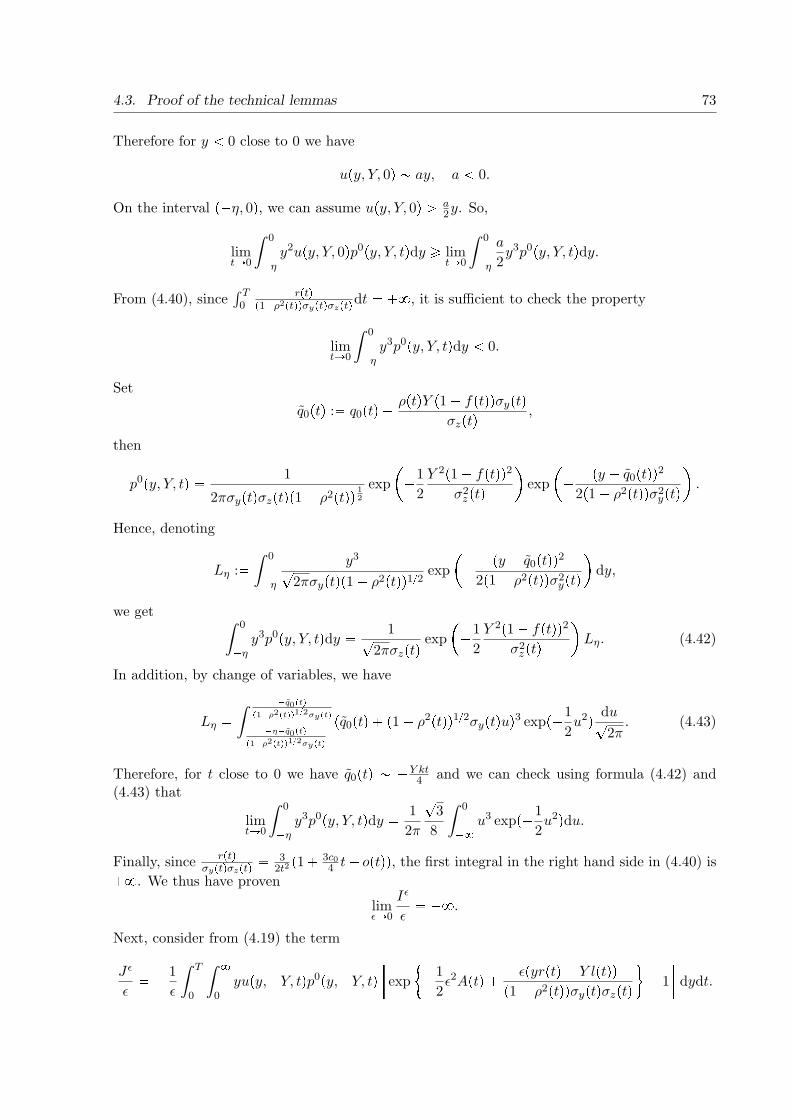
4.3. Proof of the technical lemmas 73
Therefore for y ➔ 0 close to 0 we have
u♣y, Y, 0q ✒ ay, a ➔ 0.
On the interval ♣✁η, 0q, we can assume u♣y, Y, 0q → a2y. So,
limtÑ0
ˆ 0
✁ηy2u♣y, Y, 0qp0♣y, Y, tqdy ➙ lim
tÑ0
ˆ 0
✁η
a
2y3p0♣y, Y, tqdy.
From (4.40), since´ T
0
r♣tq♣1✁ρ2♣tqqσy♣tqσz♣tqdt ✏ �✽, it is sufficient to check the property
limtÑ0
ˆ 0
✁ηy3p0♣y, Y, tqdy ➔ 0.
Set
q0♣tq :✏ q0♣tq � ρ♣tqY ♣1✁ f♣tqqσy♣tqσz♣tq ,
then
p0♣y, Y, tq ✏ 1
2πσy♣tqσz♣tq♣1✁ ρ2♣tqq 12
exp
✂✁1
2
Y 2♣1✁ f♣tqq2σ2z♣tq
✡exp
✂✁ ♣y ✁ q0♣tqq2
2♣1✁ ρ2♣tqqσ2y♣tq
✡.
Hence, denoting
Lη :✏ˆ 0
✁η
y3
❄2πσy♣tq♣1✁ ρ2♣tqq1④2 exp
✂✁ ♣y ✁ q0♣tqq2
2♣1✁ ρ2♣tqqσ2y♣tq
✡dy,
we getˆ 0
✁ηy3p0♣y, Y, tqdy ✏ 1❄
2πσz♣tqexp
✂✁1
2
Y 2♣1✁ f♣tqq2σ2z♣tq
✡Lη. (4.42)
In addition, by change of variables, we have
Lη ✏ˆ
✁q0♣tq♣1✁ρ2♣tqq1④2σy♣tq
✁η✁q0♣tq♣1✁ρ2♣tqq1④2σy♣tq
♣q0♣tq � ♣1✁ ρ2♣tqq1④2σy♣tquq3 exp♣✁1
2u2q du❄
2π. (4.43)
Therefore, for t close to 0 we have q0♣tq ✒ ✁Y kt4
and we can check using formula (4.42) and(4.43) that
limtÑ0
ˆ 0
✁ηy3p0♣y, Y, tqdy ✏ 1
2π
❄3
8
ˆ 0
✁✽u3 exp♣✁1
2u2qdu.
Finally, since r♣tqσy♣tqσz♣tq ✏ 3
2t2♣1� 3c0
4t� o♣tqq, the first integral in the right hand side in (4.40) is
�✽. We thus have proven
limǫÑ0
Iǫ
ǫ✏ �✽.
Next, consider from (4.19) the term
J ǫ
ǫ✏✁ 1
ǫ
ˆ T
0
ˆ ✽
0
yu♣y,✁Y, tqp0♣y,✁Y, tq✒exp
✧✁1
2ǫ2A♣tq � ǫ♣yr♣tq ✁ Y l♣tqq
♣1✁ ρ2♣tqqσy♣tqσz♣tq✯✁ 1
✚dydt.

74 Chapter 4. SVI with vanishing jumps
From (4.12) we have
p0♣y,✁Y, tq ✏ 1
2πσz♣tqσy♣tq♣1✁ ρ2♣tqq1④2 exp
✧✁ 1
2♣1✁ ρ2♣tqq✒♣y ✁ q0♣tqq2
σ2y♣tq
� ♣Y �m0♣tqq2σ2z♣tq
� 2ρ♣tq♣y ✁ q0♣tqq♣Y �m0♣tqqσy♣tqσz♣tq
✚✯.
Due to the term expt✁ ♣Y�m0♣tqq22♣1✁ρ2♣tqqσ2
z♣tq✉, we do not have a singularity because of σz♣tq. Indeed,
Y �m0♣tq ➙ Y ♣1✁ exp♣✁ c0π2ωqq, and for t close to 0 we have
1
σz♣tq exp
✂✁ ♣Y �m0♣tqq2
2♣1✁ ρ2♣tqqσ2z♣tq
✡
↕❛
2♣1✁ ρ2♣tqqY ♣1✁ exp♣✁ c0π
2ωqq
✄Y �m0♣tq❛
2♣1✁ ρ2♣tqqσz♣tq
☛exp
✂✁ ♣Y �m0♣tqq2
2♣1✁ ρ2♣tqqσ2z♣tq
✡
↕ C exp
✂✁ ♣Y �m0♣tqq2
4♣1✁ ρ2♣tqqσ2z♣tq
✡
where C → 0 is a constant depending on T . From the above equation and recalling the asymp-totics σy♣tq ✒
❄t for t close to 0, we deduce that the quantity
✁ˆ T
0
ˆ ✽
0
yu♣y,✁Y, tqp0♣y,✁Y, tqr ♣yr♣tq ✁ Y l♣tqq♣1✁ ρ2♣tqqσy♣tqσz♣tq sdydt
is well defined. In the same way
Hǫ
ǫ✏1
ǫ
ˆ
D
�pǫ♣y, z, T q ✁ p0♣y, z, T q✟dzdy,
has a well defined limit. Therefore, from (4.18), we deduce
u♣0, Y ✁ ǫ, 0qǫ
Ñ �✽ as ǫÑ0. (4.44)
As before, let us assume that z♣0q ✏ ✁Y � ǫ. It is easy to see that u♣✁y,✁z, tq ✏ u♣y, z, tq. Thisyields
P♣θǫ → T q ✏ u♣0, Y ✁ ǫ, tq ✏ u♣0,✁Y � ǫ, 0q,so u♣0,✁Y�ǫ,0q
ǫÑ �✽ as well. This completes the proof.

Chapter 5
Degenerate Dirichlet problems
related to the ergodic theory for an
elasto-plastic oscillator excited by a
filtered white noise
Ce chapitre fait l’objet d’un article soumis a IMA Journal of Applied Mathematics [5] en col-laboration avec Alain Bensoussan.
A stochastic variational inequality is proposed to model an elasto-plastic oscil-lator excited by a filtered white noise. We prove the ergodic properties of theprocess and characterize the corresponding invariant measure. This extendsBensoussan-Turi’s method (Degenerate Dirichlet Problems Related to the In-variant Measure of Elasto-Plastic Oscillators, AMO, 2008) with a significantadditional difficulty of increasing the dimension. Two points boundary valueproblem in dimension 1 is replaced by elliptic equations in dimension 2. Inthe present context, Khasminskii’s method (Stochastic Stability of Differen-tial Equations, Sijthoff and Noordhof,1980) leads to the study of degenerateDirichlet problems with partial differential equations and nonlocal boundaryconditions.
5.1 Introduction
Nonlinear oscillators subjected to vibrations represent useful models for predicting the responseof mechanical structures when stressed beyond the elastic limit. When the excitation is a whitenoise, it has received considerable interest over the past decades. In a previous work [7], theauthors have considered the response of a white noise excited elasto-plastic oscillator using astochastic variational inequality formulation. The results in [7] provide a framework to assessthe accuracy of calculations made in the literature (see e.g., [19, 20, 26], and the referencestherein). In this paper, instead of considering white noise input signal whose power spectraldensity (PSD) is constant, we consider an excitation with a non-constant PSD which could bea more realistic framework. We consider the excitation as the velocity of a “reflected” Ornstein-Uhlenbeck process. Therefore, comparing with the elasto plastic oscillator excited by white noise,
75

76 Chapter 5. Ergodic theory for an elasto-plastic oscillator excited by a filtered white noise
a third process occurs in the variational inequality. Consider w♣tq and w♣tq, two independentWiener processes and x♣tq an Ornstein-Ulhenbeck reflected process
dx♣tq ✏ ✁αx♣tqdt� dw♣tq � 1tx♣tq✏✁L✉dξ1t ✁ 1tx♣tq✏L✉dξ2t . (5.1)
We have ✁L ↕ x♣tq ↕ L. In this model, the stochastic excitation is given by
✁βx♣tqdt� dw♣tq.The stochastic variational inequality model is given by:✩✬✬✬✬✬✬✬✬✫
✬✬✬✬✬✬✬✬✪
dx♣tq ✏ ✁αx♣tqdt� dw♣tq � 1tx♣tq✏✁L✉dξ1t ✁ 1tx♣tq✏L✉dξ2t ,
dy♣tq ✏ ✁♣βx♣tq � c0y♣tq � kz♣tqqdt� dw♣tq,♣dz♣tq ✁ y♣tqdtq♣ζ ✁ z♣tqq ➙ 0,
⑤ζ⑤ ↕ Y,
⑤z♣tq⑤ ↕ Y.
(5.2)
When β ✘ 0, x♣tq is involved in the dynamic of y♣tq and then this model will be referred asthe 2d case. Whereas if β ✏ 0, x♣tq is not involved in the dynamic of y♣tq and then ♣y♣tq, z♣tqqsatisfy the elasto-plastic oscillator problem of [7] which will be referred as the 1d case.
Notation 5. Introduce the operators
Au :✏ 1
2uyy � 1
2uxx ✁ αxux ✁ ♣βx� c0y � kzquy � yuz,
B�u :✏ 1
2uyy � 1
2uxx ✁ αxux ✁ ♣βx� c0y � kY quy,
B✁u :✏ 1
2uyy � 1
2uxx ✁ αxux ✁ ♣βx� c0y ✁ kY quy.
The infinitesimal generator of the process ♣x♣tq, y♣tq, z♣tqq, denoted by Λ is given by:
Λ : φ ÞÑ✧Aφ if z Ps ✁ Y, Y r,B✟φ if z ✏ ✟Y,✟y → 0.
Notation 6.
O :✏ ♣✁L,Lq✂R✂♣✁Y, Y q; O� :✏ ♣✁L,Lq✂♣0,�✽q✂tY ✉; O✁ :✏ ♣✁L,Lq✂♣✁✽, 0q✂t✁Y ✉.As the main result of the paper we prove the following:
Theorem 5.1.1. There exists one and only one probability measure ν on O❨O✁❨O� satisfyingˆ
O
Aφdν �ˆ
O✁B✁φdν �
ˆ
O�B�φdν ✏ 0, ❅φ smooth.
Moreover, ν has a probability density function m such thatˆ
O
m♣x, y, zqdxdydz �ˆ
O�m♣x, y, Y qdxdy �
ˆ
O✁m♣x, y,✁Y qdxdy ✏ 1,
where

5.2. The interior Dirichlet problem 77
• tm♣x, y, zq, ♣x, y, zq P O✉ is the elastic component,
• tm♣x, y, Y q, ♣x, yq P O�✉ is the positive plastic component,
• and tm♣x, y,✁Y q, ♣x, yq P O✁✉ is the negative plastic component.
In addition, m satisfies in the sense of distributions the following equation in O,
α❇❇x rxms �
❇❇y r♣βx� c0y � kzqms ✁ y
❇m❇z � 1
2
❇2m
❇x2� 1
2
❇2m
❇y2✏ 0 in O,
and on the boundary
ym� ❇❇x rxms �
❇❇y r♣βx� c0y � kY qms � 1
2
❇2m
❇x2� 1
2
❇2m
❇y2✏ 0, in O�
✁ym� ❇❇x rxms �
❇❇y r♣βx� c0y ✁ kY qms � 1
2
❇2m
❇x2� 1
2
❇2m
❇y2✏ 0, in O✁
m ✏ 0, in ♣✁L,Lq ✂ ♣✁✽, 0q ✂ tY ✉ ❨ ♣✁L,Lq ✂ ♣0,✽q ✂ t✁Y ✉.
The proof will be based on solving a sequence of interior and exterior Dirichlet problems,which are interesting in themselves. We will put in parallel the 1d and 2d cases, in order tofacilitate the reader’s work. In the 1d case, the variable x disappears (β ✏ 0), we will still usethe notation A,B�, B✁ for the operators defined above without x.
Let us mention that our study presents a mathematical interest because it generalizes themethod proposed by the first author and J. Turi [7] in the case of higher dimension. Non-localboundary conditions expressed in the form of differential equations in dimension 1 are replacedby elliptic partial differential equations (PDEs) in dimension 2. In the first case, there are twosemi-explicit solutions. Thus, the non-local boundary conditions are reduced to two unknownnumbers. In the second case, we do not know explicit formulas for solutions of the both ellipticon the boundary. In this context, these two solutions depend on two unknown functions respec-tively defined on the set ♣✁L,Lq.
In addition, the choice of the excitation (5.1) is also motivated by two technical considerations:
• the first is to force x♣tq (through the processes ξ1, ξ2) to evolve in the compact set r✁L,Ls.Thus, as part of our proof, a compactness argument allows to show the ergodic propertyof the triple ♣x♣tq, y♣tq, z♣tqq. Note that this is not a problem in terms of applications,because if we choose L large enough, then the process x♣tq is similar to an Ornstein-Ulhenbeck process.
• the second is the uncorrelation of w♣tq and w♣tq. In our approach, based on PDEs as-sociated to the triple ♣x♣tq, y♣tq, z♣tqq, we avoid the appearance of cross-derivative termsin the infinitesimal generator Λ. In the case where w♣tq and w♣tq are correlated, thesecross-derivative terms yield more technical difficulties.
5.2 The interior Dirichlet problem
In this section, we prove existence and uniqueness to the homogeneous interior Dirichlet problem.

78 Chapter 5. Ergodic theory for an elasto-plastic oscillator excited by a filtered white noise
5.2.1 Some background on the interior Dirichlet problem in the 1d case
Let us recall the interior Dirichlet problem from [7]. Let y1 → 0,
Notation 7.
D1 :✏ ♣✁y1, y1q ✂ ♣✁Y, Y q; D�1 :✏ ♣0, y1q ✂ tY ✉; D✁
1 :✏ ♣✁y1, 0q ✂ t✁Y ✉
and
Dǫ1 :✏ ♣✁y1 � ǫ, y1 ✁ ǫq ✂ ♣✁Y, Y q, ǫ → 0.
Denote τ1 :✏ inftt → 0, ⑤y♣tq⑤ ✏ y1✉ and consider φ P L✽♣✁Y, Y q. We will use the followingnotation Ep♣☎q :✏ Et☎ ⑤♣y♣0q, z♣0qq ✏ p✉. It is shown that E♣y,zq♣φ♣z♣τ1qqq solves a nonlocalDirichlet problem: Find η P L✽♣D1q ❳ C0♣Dǫ
1q,❅ǫ → 0 such that
Aη ✏ 0 in D1, B�η ✏ 0 in D�1 , B✁η ✏ 0 in D✁
1 (5.3)
with
η♣y1, zq ✏ φ♣zq, η♣✁y1, zq ✏ 0, if z P ♣✁Y, Y q.Since η♣y1, Y q ✏ φ♣Y q and η♣✁y1,✁Y q ✏ 0, there are semi-explicit solutions by solving ordinarydifferential equations for η on the boundary at z ✏ Y , and z ✏ ✁Y respectively,
η♣y, Y q ✏ ηY I♣y, y1q � φ♣Y qI♣0, yq, 0 ➔ y ↕ y1; η♣y,✁Y q ✏ η✁Y I♣✁y1, yq, ✁y1 ↕ y ➔ 0,
where ηY and η✁Y are constants, and
I♣a, bq :✏´ b
aexp♣c0λ2 � 2kY λqdλ
´ y10
exp♣c0λ2 � 2kY λqdλ.
The nonlocal condition is restricted to the value of these two constants. Based on these semi-explicit expressions a subset K of H1♣D1q is defined for proving existence of the solution to (5.3), by
K :✏
✩✬✬✬✬✬✬✬✬✫✬✬✬✬✬✬✬✬✪
v P H1♣D1q,v♣✁y1, zq ✏ φ♣zq, v♣✁y1, zq ✏ 0,
v♣y, Y q ✏ vY I♣y, y1q � φ♣Y qI♣0, yq, 0 ↕ y ↕ y1
v♣y,✁Y q ✏ v✁Y I♣✁y1, yq, ✁y1 ↕ y ↕ 0
vY , v✁Y are constant with ⑤v✟Y ⑤ ↕ ⑥φ⑥L✽ .The set K is convex and not empty if φ♣zq P H1♣✁Y, Y q. We take v♣y, zq ✏ φ♣zqI♣0, yq1ty→0✉.
5.2.2 The interior Dirichlet problem in the 2d case
Notation 8.
∆1 :✏ ♣✁L,Lq ✂ ♣✁y1, y1q ✂ ♣✁Y, Y q,∆�
1 :✏ ♣✁L,Lq ✂ ♣0, y1q ✂ tY ✉, ∆✁1 :✏ ♣✁L,Lq ✂ ♣✁y1, 0q ✂ t✁Y ✉
and
∆ǫ1 :✏ ♣✁L,Lq ✂ ♣✁y1 � ǫ, y1 ✁ ǫq ✂ ♣✁Y, Y q,❅ǫ → 0.
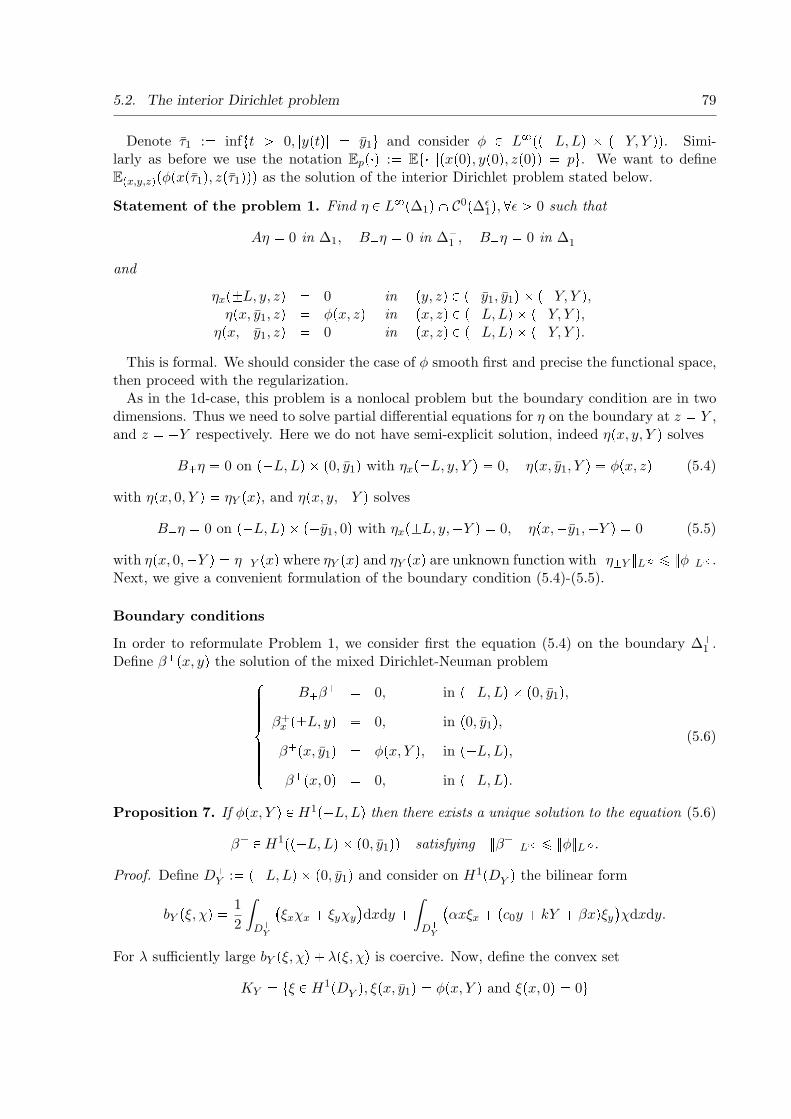
5.2. The interior Dirichlet problem 79
Denote τ1 :✏ inftt → 0, ⑤y♣tq⑤ ✏ y1✉ and consider φ P L✽♣♣✁L,Lq ✂ ♣✁Y, Y qq. Simi-larly as before we use the notation Ep♣☎q :✏ Et☎ ⑤♣x♣0q, y♣0q, z♣0qq ✏ p✉. We want to defineE♣x,y,zq♣φ♣x♣τ1q, z♣τ1qqq as the solution of the interior Dirichlet problem stated below.
Statement of the problem 1. Find η P L✽♣∆1q ❳ C0♣∆ǫ1q,❅ǫ → 0 such that
Aη ✏ 0 in ∆1, B�η ✏ 0 in ∆�1 , B✁η ✏ 0 in ∆✁
1
and
ηx♣✟L, y, zq ✏ 0 in ♣y, zq P ♣✁y1, y1q ✂ ♣✁Y, Y q,η♣x, y1, zq ✏ φ♣x, zq in ♣x, zq P ♣✁L,Lq ✂ ♣✁Y, Y q,
η♣x,✁y1, zq ✏ 0 in ♣x, zq P ♣✁L,Lq ✂ ♣✁Y, Y q.This is formal. We should consider the case of φ smooth first and precise the functional space,
then proceed with the regularization.As in the 1d-case, this problem is a nonlocal problem but the boundary condition are in two
dimensions. Thus we need to solve partial differential equations for η on the boundary at z ✏ Y ,and z ✏ ✁Y respectively. Here we do not have semi-explicit solution, indeed η♣x, y, Y q solves
B�η ✏ 0 on ♣✁L,Lq ✂ ♣0, y1q with ηx♣✟L, y, Y q ✏ 0, η♣x, y1, Y q ✏ φ♣x, zq (5.4)
with η♣x, 0, Y q ✏ ηY ♣xq, and η♣x, y,✁Y q solves
B✁η ✏ 0 on ♣✁L,Lq ✂ ♣✁y1, 0q with ηx♣✟L, y,✁Y q ✏ 0, η♣x,✁y1,✁Y q ✏ 0 (5.5)
with η♣x, 0,✁Y q ✏ η✁Y ♣xq where ηY ♣xq and ηY ♣xq are unknown function with ⑥η✟Y ⑥L✽ ↕ ⑥φ⑥L✽ .Next, we give a convenient formulation of the boundary condition (5.4)-(5.5).
Boundary conditions
In order to reformulate Problem 1, we consider first the equation (5.4) on the boundary ∆�1 .
Define β�♣x, yq the solution of the mixed Dirichlet-Neuman problem✩✬✬✬✬✬✬✫✬✬✬✬✬✬✪
B�β� ✏ 0, in ♣✁L,Lq ✂ ♣0, y1q,β�x ♣✟L, yq ✏ 0, in ♣0, y1q,β�♣x, y1q ✏ φ♣x, Y q, in ♣✁L,Lq,β�♣x, 0q ✏ 0, in ♣✁L,Lq.
(5.6)
Proposition 7. If φ♣x, Y q P H1♣✁L,Lq then there exists a unique solution to the equation (5.6)
β� P H1♣♣✁L,Lq ✂ ♣0, y1qq satisfying ⑥β�⑥L✽ ↕ ⑥φ⑥L✽ .
Proof. Define D�Y :✏ ♣✁L,Lq ✂ ♣0, y1q and consider on H1♣D�
Y q the bilinear form
bY ♣ξ, χq ✏ 1
2
ˆ
D�Y
�ξxχx � ξyχy
✟dxdy �
ˆ
D�Y
�αxξx � ♣c0y � kY � βxqξy
✟χdxdy.
For λ sufficiently large bY ♣ξ, χq � λ♣ξ, χq is coercive. Now, define the convex set
KY ✏ tξ P H1♣D�Y q, ξ♣x, y1q ✏ φ♣x, Y q and ξ♣x, 0q ✏ 0✉

80 Chapter 5. Ergodic theory for an elasto-plastic oscillator excited by a filtered white noise
which is not empty since φ♣x, Y q P H 12 ♣✁L,Lq. Take z P KY with ⑥z⑥L✽ ↕ ⑥φ⑥L✽ , we define ξλ
to be the unique solution of
bY ♣ξλ, χ✁ ξλq � λ♣ξλ, χ✁ ξλq ➙ λ♣z, χ✁ ξλq, ξλ P KY ,❅χ P KY (5.7)
We have defined a map Tλ♣zq ✏ ξλ from KY Ñ KY . Let us check that
⑥ξλ⑥L✽ ↕ ⑥φ⑥L✽ ✏ C. (5.8)
Indeed, in (5.7) we take χ ✏ ξλ ✁ ♣ξλ ✁ Cq� P KY . Hence
✁bY ♣ξλ, ♣ξλ ✁ Cq�q ✁ λ♣ξλ, ♣ξλ ✁ Cq�q ➙ λ♣z, ♣ξλ ✁ Cq�qand
bY ♣♣ξλ ✁ Cq�, ♣ξλ ✁ Cq�q � λ⑤♣ξλ ✁ Cq�⑤L2 ↕ ✁λ♣z � C, ♣ξλ ✁ Cq�q.Since z � C ➙ 0 it follows that ♣ξλ ✁ Cq� ✏ 0, hence ξλ ↕ C. Similarly, we check that♣✁ξλ ✁ Cq� ✏ 0, hence we have (5.8). Consider then the sequence ξnλ defined by
bY ♣ξn�1λ , χ✁ ξn�1
λ q � λ♣ξn�1λ , χ✁ ξn�1
λ q ➙ λ♣ξnλ , χ✁ ξn�1λ q (5.9)
withξ0λ P KY , ⑥ξ0λ⑥L✽ ↕ ⑥φ⑥L✽ .
We can take ξ0λ♣x, yq ✏ yy1φ♣x, Y q. From (5.8), we have ⑥ξnλ⑥L✽♣D�Y q ↕ C and from (5.9), we have
⑥ξnλ⑥H1♣D�Y q ↕ C ✶. Then, we can consider a subsequence, also denoted by ξnλ such that
ξnλ Ñ ξ in H1♣D�Y q weakly and in L✽♣D�
Y q weakly ✍also,
ξnλ Ñ ξ in L2♣D�Y q strongly.
From (5.9) we obtainbY ♣ξ, χ✁ ξq ➙ 0, ξ P KY ,❅χ P KY .
We conclude easily that ξ is a solution of (5.6) also ⑥ξ⑥L✽ ↕ ⑥φ⑥L✽ . Now, in order to proveuniqueness, we must prove that a solution ξ P H1♣D�
Y q satisfying
B�ξ ✏ 0 in ♣✁L,Lq ✂ ♣0, y1qξx♣✁L, yq ✏ ξx♣L, yq ✏ 0
ξ♣x, y1q ✏ ξ♣x, 0q ✏ 0
(5.10)
is identically zero.Consider χ :✏ ξx then we have
B�χ� αχ� βξy ✏ 0 in D�Y ,
χ♣✁L, yq ✏ χ♣L, yq ✏ 0,
χ♣x, y1q ✏ χ♣x, 0q ✏ 0,
hence χ P H10 ♣D�
Y q. This implies
ξxx P L2♣D�Y q, ξyx P L2♣D�
Y q.From equation (5.10) we deduce ξyy P L2♣D�
Y q. Hence ξ P H2♣D�Y q. In particular, ξ is continuous
on D�Y . We have ⑥ξ⑥L✽ ✏ 0, so ξ ✏ 0.

5.2. The interior Dirichlet problem 81
Now, consider the following convex sets,
KY,M :✏ tχ� P H1♣♣✁L,Lq✂♣0, y1qq satisfying ♣5.12q; χ�♣x, y1q ✏ 0; ⑥χ�⑥L✽ ↕M✉ (5.11)
where
´ L
✁L´ y10t1
2♣χ�x ψx � χ�y ψyq � ♣αxχ�x � ♣βx� c0y � kY qχ�y qψ✉dxdy ✏ 0,
❅ψ P H1♣♣✁L,Lq ✂ ♣0, y1qq with ψ♣x, 0q ✏ ψ♣x, y1q ✏ 0.(5.12)
and
K✁Y,M :✏ tχ✁ P H1♣♣✁L,Lq ✂ ♣✁y1, 0qq satisfying ♣5.14q; χ✁♣x,✁y1q ✏ 0; ⑥χ✁⑥L✽ ↕M✉(5.13)
where
´ L
✁L´ 0
✁y1t12♣χ✁x ψx � χ✁y ψyq � ♣αxχ✁x � ♣βx� c0y ✁ kY qχ✁y qψ✉dxdy ✏ 0,
❅ψ P H1♣♣✁L,Lq ✂ ♣✁y1, 0qq with ψ♣x, 0q ✏ ψ♣x,✁y1q ✏ 0.(5.14)
These sets are not empty since they contain 0.
Remark 7. • ❅π♣yq function of y such that π♣0q ✏ 0 ,
tχπ; χ P KY,M✉ and tχπ; χ P K✁Y,M✉ are H1 ✁ bounded.
• If χ P KY,⑥φ⑥L✽ , denoting ω :✏ β� � χ, we have
B�ω ✏ 0 and max♣⑤ω♣x, 0q⑤, ⑤ω♣x, y1q⑤q ↕ ⑥φ⑥L✽ ,
so a maximum principle implies ⑥ω⑥L✽ ↕ ⑥φ⑥L✽.
Using the sets KY,⑥φ⑥ and K✁Y,⑥φ⑥, the following result gives a convenient formulation of theboundary conditions in Problem 1.
Proposition 8. The Problem 1 can be reformulated in the following way: find η P L✽♣∆1q ❳C0♣∆ǫ
1q,❅ǫ → 0 such that
Aη ✏ 0 in ∆1, η♣x, y, Y q ✁ β�♣x, yq P KY,⑥φ⑥, η♣x, y,✁Y q P K✁Y,⑥φ⑥and
ηx♣✟L, y, zq ✏ 0, in ♣y, zq P ♣✁y1, y1q ✂ ♣✁Y, Y q,η♣x, y1, zq ✏ φ♣x, zq, in ♣x, zq P ♣✁L,Lq ✂ ♣✁Y, Y q,
η♣x,✁y1, zq ✏ 0, in ♣x, zq P ♣✁L,Lq ✂ ♣✁Y, Y q.
Proof. First, we can obtain the generic solution of (5.4) by considering any function χ� whichsatisfies
χ� P H1♣♣✁L,Lq ✂ ♣0, y1qq

82 Chapter 5. Ergodic theory for an elasto-plastic oscillator excited by a filtered white noise
and
B�χ� ✏ 0, χ�x ♣✟L, yq ✏ 0, χ�♣x, y1q ✏ 0. (5.15)
Note that we have not defined the value of χ� for y ✏ 0, hence χ� is certainly not unique. Weadd the condition that χ� is bounded by ⑥φ⑥L✽ . We define in a similar way the function χ✁
such that
χ✁ P H1♣♣✁L,Lq ✂ ♣✁y1, 0qqand
B✁χ✁ ✏ 0, χ✁x ♣✟L, yq ✏ 0, χ✁♣x,✁y1q ✏ 0. (5.16)
Then, interpreting (5.15) as (5.12) and (5.16) as (5.14) repectively, we obtain χ� P KY,⑥φ⑥ andχ✁ P K✁Y,⑥φ⑥. Hence, the set of solutions of (5.4) and (5.5) can be written as follows
η♣x, y, Y q ✁ β�♣x, yq P KY,⑥φ⑥, y → 0; η♣x, y,✁Y q P K✁Y,⑥φ⑥, y ➔ 0.
Approximation (part 1)
We study Problem 1 by a regularization method in the next proposition. Define Aǫ :✏ A� ǫ2❇2❇z2 .
Proposition 9. The following problem: find ηǫ P L✽♣∆1q❳H1♣∆1q such that ⑥ηǫ⑥L✽ ↕ ⑥φ⑥L✽,
Aǫηǫ ✏ 0 in ∆1, ηǫ♣x, y, Y q ✁ β�♣x, yq P KY,⑥φ⑥, ηǫ♣x, y,✁Y q P K✁Y,⑥φ⑥ (5.17)
and
ηǫx♣✟L, y, zq ✏ 0, in ♣y, zq P ♣✁y1, y1q ✂ ♣✁Y, Y q,ηǫz♣x, y,✟Y q ✏ 0, in ♣x,✠yq P ♣✁L,Lq ✂ ♣0, y1q,ηǫ♣x, y1, zq ✏ φ♣x, zq, in ♣x, zq P ♣✁L,Lq ✂ ♣✁Y, Y q,ηǫ♣x,✁y1, zq ✏ 0, in ♣x, zq P ♣✁L,Lq ✂ ♣✁Y, Y q,
has a unique solution.
As in the 1d case, we formulate a variational inequality to prove existence of solutions. In thepresent context, we consider a convex subset of H1♣∆1q which is adapted to the two dimensionalboundary condition by
K ✏
✩✬✬✬✬✫✬✬✬✬✪
ψ P H1♣∆1q, ⑥ψ⑥✽ ↕ ⑥φ⑥✽,ψ♣x, y1, zq ✏ φ♣x, zq, for ♣x, zq P ♣✁L,Lq ✂ ♣✁Y, Y q,ψ♣x,✁y1, zq ✏ 0, for ♣x, zq P ♣✁L,Lq ✂ ♣✁Y, Y q,ψ♣., ., Y q ✁ β�♣x, yq P KY,⑥φ⑥L✽ ,ψ♣., .,✁Y q P K✁Y,⑥φ⑥L✽ .
Proposition 10. The set K is a closed non-empty subset of H1♣∆1q.
Proof. The fact that K is closed follows from the continuity of the trace operator. Now, pickthe function,
ψ♣x, y, zq ✏ y
y1
✏φ♣x, zq ✁ z
2Yφ♣x, Y q ✁ 1
2φ♣x, Y q✘1ty➙0✉ � ♣
z
2Y� 1
2qβ�♣x, yq1ty➙0✉. (5.18)

5.2. The interior Dirichlet problem 83
We have
ψ♣x, y1, zq ✏ φ♣x, zq,ψ♣x,✁y1, zq ✏ 0,
ψ♣x, y, Y q ✏ β�♣x, yq, y → 0,
ψ♣x, y,✁Y q ✏ 0, y ➔ 0.
So, if φ♣x, zq P H1♣❇∆1q, φ♣x, Y q P H1♣✁L,Lq, then the function ψ defined by (5.16) belongs toK.
Remark 8. If u P K and w P H1♣∆1q with w♣x,✟y1, zq ✏ 0 and w♣x, y,✟Y q ✏ 0, for 0 ➔ ✟y ➔y1 then u� w P K.
Consider the bilinear form
a♣u, vq ✏ 1
2
ˆ
∆1
tǫuzvz � uyvy � uxvx✉dxdydz
�ˆ
∆1
♣βx� c0y � kzquyvdxdydz ✁ˆ
∆1
yuzvdxdydz �ˆ
∆1
αxuxvdxdydz.
Equation (5.17) is formulated as follows a♣u, v ✁ uq ➙ 0, ❅v P K,u P K.
Proof of Proposition 9. First, existence is proved by variational argument. For λ sufficientlylarge a♣u, vq � λ♣u, vq is coercive on H1♣∆1q and for f P L2♣∆1q we can solve the variationalinequality
a♣u, v ✁ uq � λ♣u, v ✁ uq ➙ ♣f, v ✁ uq, ❅v P K,u P K.We define the map u ✏ Tλw where u is the unique solution of
a♣u, v ✁ uq � λ♣u, v ✁ uq ➙ λ♣w, v ✁ uq, ❅v P K,u P K.
The following lemma shows that Tλ is a contracting map. (see proof in Appendix)
Lemma 5. If ⑥w⑥L✽ ↕ ⑥φ⑥L✽ then ⑥u⑥L✽ ↕ ⑥φ⑥L✽.
Moreover, taking v ✏ u0 P K we deduce
a♣u, uq � λ⑤u⑤2L2 ↕ a♣u, u0q � λ♣u, u0q � λγ⑤u0 ✁ u⑤L1 .
That implies
⑥u⑥H1♣∆1q ↕M,
for a constant M which depends only of λ, ǫ, H1 norm of u0 and γ.Now, we define
K ✏ tw P K : ⑥w⑥L✽ ↕ ⑥φ⑥L✽ , ⑥w⑥H1 ↕M✉.We have Tλ : L2♣∆1q Ñ L2♣∆1q is continuous, maps K into itself and K is a compact subset ofL2. Then Schauder’s theorem implies Tλ has a fixed point u P K which satisfies
a♣u, v ✁ uq ➙ 0, ❅v P K.

84 Chapter 5. Ergodic theory for an elasto-plastic oscillator excited by a filtered white noise
Let us check that u is solution of (5.17). As u P K, we have
B�u ✏ 0 in ∆�
B✁u ✏ 0 in ∆✁
u♣x, y1, zq ✏ φ♣x, zq in ♣✁L,Lq ✂ ♣✁Y, Y qu♣x,✁y1, zq ✏ 0 in ♣✁L,Lq ✂ ♣✁Y, Y q
Moreover,
❅v P H :✏✧v P H1♣∆1q such that
✧v♣x,✟y1, zq ✏ 0v♣x, y,✟Y q ✏ 0, 0 ➔ ✟y ➔ y1
✯,
we have u� v P K and a♣u, vq ➙ 0. Then,
Aǫu ✏ 0 in the sense H✶
and integration by parts gives
ǫ
2
ˆ L
✁L
ˆ 0
✁y1uz♣x, y, Y qv♣x, y, Y qdxdy ✁ ǫ
2
ˆ L
✁L
ˆ y1
0
uz♣x, y,✁Y qv♣x, y,✁Y qdxdy
�ˆ y1
✁y1
ˆ Y
✁Yux♣L, y, zqv♣L, y, zqdydz ✁
ˆ y1
✁y1
ˆ Y
✁Yux♣✁L, y, zqv♣✁L, y, zqdydz ✏ 0.
Uniqueness of the solution to problem (5.17) comes from ⑥u⑥L✽ ↕ ⑥φ⑥L✽ .
Approximation (part 2)
When φ is smooth, we can exhibit a solution to the problem (5.19) by extracting a convergingsubsequence of ηǫ. Let θ a smooth fonction such that θ♣✟y1q ✏ 0. Denote π♣yq :✏ ypθ♣yqq forsome p, q.
Proposition 11. The following problem: find η P L✽♣∆1q such that ηπ P H1♣∆1q,Aη ✏ 0 in ∆1, η♣x, y, Y q ✁ β�♣x, yq P KY,⑥φ⑥, η♣x, y,✁Y q P K✁Y,⑥φ⑥ (5.19)
and
ηx♣✟L, y, zq ✏ 0 in ♣y, zq P ♣✁y1, y1q ✂ ♣✁Y, Y q,η♣x, y1, zq ✏ φ♣x, zq in ♣x, zq P ♣✁L,Lq ✂ ♣✁Y, Y q,η♣x,✁y1, zq ✏ 0 in ♣x, zq P ♣✁L,Lq ✂ ♣✁Y, Y q,
has a unique solution.
As in the 1d case, the key ingredient of the proof is to bound uniformly the norm of firstderivative w.r.t. z using the auxiliary function π.
Proof. From the previous section, we have ⑥ηǫ⑥✽ ↕ ⑥φ⑥✽, hence ηǫ Ñ η in L✽✍. We also havea♣ηǫ, u0 ✁ ηǫq ➙ 0, for some u0 P K. So, we deduce estimates in the following lemma: (see proofin Appendix)
Lemma 6. We have
ǫ
ˆ
∆1
♣ηǫzq2dxdydz ↕ C;
ˆ
∆1
♣ηǫxq2dxdydz ↕ C;
ˆ
∆1
♣ηǫyq2dxdydz ↕ C.

5.2. The interior Dirichlet problem 85
It is licit to test (5.17) with ηǫzy2p✁1θ2q. We have
ˆ
∆1
� ǫ2ηǫzz �
1
2ηǫyy �
1
2ηǫxx � yηǫz ✁ αxηǫx ✁ ♣βx� c0y � kzqηǫy
✟ηǫzy
2p✁1θ2q ✏ 0.
So, we obtain
´
∆1♣ηǫzπq2 ↕
14
´ L
0
´ y10t♣ηǫy♣x, y, Y qq2 � ♣ηǫx♣x, y, Y qq2✉y2p✁1θ2qdxdy
� 14
´ L
0
´ 0
✁y1t♣ηǫy♣x, y,✁Y qq2 � ♣ηǫx♣x, y,✁Y qq2✉⑤y⑤2p✁1θ2qdxdy
� 12
´
∆1ηǫyη
ǫz
�♣♣2p✁ 1qy2p✁2θ2q � y2p✁12qθ✶θ2q✁1q � 2♣βx� c0y � kzqy2p✁1θ2q✟dxdydz
� ´
∆1ηǫxη
ǫz♣αxy2p✁1θ2qqdxdydz.
(5.20)Moreover, Remark 7 allows to bound the two integrals on the boundary that yields the followingestimate:
⑥ηǫzπ⑥L2 ↕ Cπ.
Denoting vǫ :✏ ηǫπ, we have ⑥vǫ⑥H1♣∆1q ↕ Cπ so we can extract a weakly converging subse-quence vǫ Ñ v in H1♣∆1q and v ✏ ηπ P H1♣∆1q. We can check that η satisfies the boundarycondition of Problem 1. First, let us check that
π♣yqAη ✏ 0 in H✁1♣∆1q, π♣yqηx♣✟L, y, zq ✏ 0 in ♣H 12 ♣♣✁L,Lq ✂ ♣✁y1, y1qqq✶.
As vǫ P H2♣∆1q and πAǫηǫ ✏ 0, we have
✁Aǫvǫ ✏ f♣η, ηyq in strong sense
with f♣η, ηyq :✏ ✁12tπ✷ηǫ � 2π✶ηǫy✉ � ♣c0y � kz � αxqπ✶ηǫ.
We obtain that ❅φ P H1♣∆1q, φ♣x, y,✟Y q ✏ 0 and φ♣x,✟y1, zq ✏ 0,
ǫ
2
ˆ
∆1
vǫzφz�1
2
ˆ
∆1
vǫyφy�1
2
ˆ
∆1
vǫxφx�ˆ
∆1
�αxvǫx�♣βx� c0y�kzqvǫy✁ yvǫz
✟φ ✏ˆ
∆1
f♣ηǫ, ηǫyqφ.
Now, when ǫ goes to 0, we have
1
2
ˆ
∆1
vyφy � 1
2
ˆ
∆1
vxφx �ˆ
∆1
�αxvx � ♣βx� c0y � kzqvy ✁ yvz
✟φ ✏ˆ
∆1
f♣η, ηyqφ.
We deduce we have in H✁1♣∆1q, firstly ✁Av ✏ f♣η, ηyq which is equivalent to πAη ✏ 0 and
secondly that choice of test function implies πηx♣✟L, y, zq ✏ 0 in ♣H 12 ♣♣✁L,Lq ✂ ♣✁y1, y1qq✶.
Then, we check that
η♣x, y, Y q ✁ β�♣x, yq P KY,⑥φ⑥; η♣x, y,✁Y q P K✁Y,⑥φ⑥.
We know that ηǫ P H1♣∆1q, its trace is well defined and satisfies
γ♣ηǫq♣x, y, Y q ✏ χ�,ǫ � β�; χ�,ǫ P KY,⑥φ⑥; y → 0
γ♣ηǫq♣x, y,✁Y q ✏ χ✁,ǫ; χ✁,ǫ P K✁Y,⑥φ⑥; y ➔ 0

86 Chapter 5. Ergodic theory for an elasto-plastic oscillator excited by a filtered white noise
with
⑥χ✟,ǫ⑥L✽ ↕ ⑥φ⑥L✽ . (5.21)
We also have χ✁,ǫ, χ�,ǫ satisfy respectively (5.22) and (5.23)
´ L
✁L´ y10t1
2♣χ�,ǫx ψx � χ
�,ǫy ψyq � ♣αxχ�,ǫx � ♣βx� c0y � kY qχ�,ǫy qψ✉dxdy ✏ 0,
❅ψ P H1♣♣✁L,Lq ✂ ♣0, y1qq with ψ♣x, 0q ✏ ψ♣x, y1q ✏ 0.(5.22)
and
´ L
✁L´ 0
✁y1t12♣χ✁,ǫx ψx � χ
✁,ǫy ψyq � ♣αxχ✁,ǫx � ♣βx� c0y ✁ kY qχ✁,ǫy qψ✉dxdy ✏ 0,
❅ψ P H1♣♣✁L,Lq ✂ ♣✁y1, 0qq with ψ♣x, 0q ✏ ψ♣x,✁y1q ✏ 0.(5.23)
First, we study convergence of the sequence χ✟,ǫ and we deduce the PDEs satisfied by limǫÑ0 χ✟,ǫ.
In particular (5.21) implies
χ�,ǫ Ñ χ� in L2♣♣✁L,Lq ✂ ♣0, y1qq weakly,
χ✁,ǫ Ñ χ✁ in L2♣♣✁L,Lq ✂ ♣✁y1, 0qq weakly.
And (5.22) and (5.23) imply
⑥χ�,ǫπ⑥H1 ↕ C and χ�,ǫπ Ñ χ�π in H1 weakly,
⑥χ✁,ǫπ⑥H1 ↕ C and χ✁,ǫπ Ñ χ✁π in H1 weakly.
Denote ξ✟,ǫ :✏ χ✟,ǫy2. From (5.22), we obtainB�ξ�,ǫ ✏ 0 in ♣✁L,Lq✂♣✁y1, y1q, inH✁1♣♣✁L,Lq✂♣0, y1qq. Since the operator B� is strictly elliptic then ξ�,ǫ P H2♣♣✁L,Lq✂♣0, y1qq. We also have
ξ�,ǫx ♣✟L, yq ✏ 0 in ♣H 1
2 ♣0, y1qq✶. As ξ�,ǫ P H2♣∆1q and πB�χ�,ǫ ✏ 0, we obtain
✁B�ξ�,ǫ ✏ g♣χ�,ǫ, χ�,ǫy q in a strong sense
with g♣χ�,ǫ, χ�,ǫy q :✏ ✁χ�,ǫt1✁2y♣αx�c0y�kY q✉✁2yχ�,ǫy . We obtain that ❅ψ P H1♣♣✁L,Lq✂♣0, y1qq, ψ♣x, 0q ✏ ψ♣x, y1q ✏ 0,
ˆ L
✁L
ˆ y1
0
1
2♣ξ�,ǫx ψx � ξ�,ǫy ψyq �
�αxξ�,ǫx � ♣βx� c0y � kY qξ�,ǫy ✁ yξ�,ǫz
✟ψ ✏
ˆ L
✁L
ˆ y1
0
g♣χǫ, χǫyqψ.
Now, when ǫ goes to 0, we have
ˆ L
✁L
ˆ y1
0
1
2♣ξ�x ψx � ξ�y ψyq �
�αxξ�x � ♣βx� c0y � kY qξ�y ✁ yξ�z
✟ψ ✏
ˆ L
✁L
ˆ y1
0
g♣χ, χyqψ.
We deduce that in H✁1♣♣✁L,Lq ✂ ♣0, y1qq, we firstly have ✁B�ξ� ✏ g♣χ�, χ�y q, which is equiv-alent to y2B�χ� ✏ 0 and secondly that choice of test functions implies y2χ�x ♣✟L, yq ✏ 0 in
♣H 12 ♣♣0, y1qqq✶. To summarize, we have
ξ� P H1♣♣✁L,Lq ✂ ♣0, y1qq

5.2. The interior Dirichlet problem 87
and ✩✬✬✬✫✬✬✬✪
✁B�ξ� ✏ g♣χ�, χ�y q in ♣✁L,Lq ✂ ♣0, y1q,ξ�x ♣✟L, yq ✏ 0 in ♣0, y1q,ξ�♣x, y1q ✏ 0 in ♣✁L,Lq.
Henceπχ� P H1♣♣✁L,Lq ✂ ♣0, y1qq, ⑥χ�⑥L✽ ↕ ⑥φ⑥L✽
and ✩✬✬✬✫✬✬✬✪
πB�χ� ✏ 0 in ♣✁L,Lq ✂ ♣0, y1q,πχ�x ♣✟L, yq ✏ 0 in ♣0, y1q,χ�♣x, y1q ✏ 0 in ♣✁L,Lq.
(5.24)
Similarly, we haveπχ✁ P H1♣♣✁L,Lq ✂ ♣✁y1, 0qq, ⑥χ✁⑥L✽ ↕ ⑥φ⑥L✽
and ✩✬✬✬✫✬✬✬✪
πB�χ✁ ✏ 0 in ♣✁L,Lq ✂ ♣✁y1, 0q,πχ✁x ♣✟L, yq ✏ 0 in ♣✁y1, 0q,πχ✁♣x,✁y1q ✏ 0 in ♣✁L,Lq.
(5.25)
First, γ♣πηǫq Ñ π♣χ� � β�q in H1♣♣✁L,Lq ✂ ♣0, y1qq weakly. Secondly, the weak convergence
of πηǫ Ñ πη in H1♣∆1q implies the weak convergence of γ♣πηǫq Ñ γ♣πηq in H12 ♣❇∆1q. By
uniqueness of the limit, we deduce γ♣πηq ✏ π♣χ� � β�q. Finally, we verify that
η♣x, y1, zq ✏ φ♣x, zq; η♣x, y1, zq ✏ 0.
Using Green formula, we obtain
❅ψ P H1♣∆1q,ˆ
∆1
ηǫyψ �ˆ
∆1
ηǫψy ✏ˆ
❇∆1
φψ~n♣yqdσ.
Now, we can let ǫ tend to 0, we obtain
❅ψ P H1♣∆1q,ˆ
∆1
ηyψ �ˆ
∆1
ηψy ✏ˆ
❇∆1
φψ~n♣yqdσ.
Approximation (part 3)
Now, φ P L✽♣❇∆1q, we introduce a sequence of function tφk, k ➙ 0✉ ⑨ H1♣❇∆1q such thatφk Ñ φ in L2♣❇∆1q. We denote ηk the solution of the Problem 5.19 with φk as boundarycondition. From the previous section we have ηk P L✽♣∆1q satisfies π♣yqηk P H1♣∆1q,
Aηk ✏ 0 in ∆1, ηk♣x, y, Y q ✁ βk,�♣x, yq P KY,⑥φ⑥, ηk♣x, y,✁Y q P K✁Y,⑥φ⑥
and
ηkx♣✟L, y, zq ✏ 0 in ♣y, zq P ♣✁y1, y1q ✂ ♣✁Y, Y q,ηk♣x, y1, zq ✏ φk♣x, zq in ♣x, zq P ♣✁L,Lq ✂ ♣✁Y, Y q,
ηk♣x,✁y1, zq ✏ 0 in ♣x, zq P ♣✁L,Lq ✂ ♣✁Y, Y q.

88 Chapter 5. Ergodic theory for an elasto-plastic oscillator excited by a filtered white noise
where βk,�♣x, yq P H1♣♣✁L,Lq ✂ ♣0, y1qq solves the problem (5.6) with φk♣x, Y q as boundarycondition. Moreover ⑥ηk⑥✽ ↕ ⑥φ⑥✽ and ⑥βk⑥✽ ↕ ⑥φ⑥✽. Let us check that the sequence βk hasa limit.
Proposition 12. We have
βk,�♣x, yq Ñ β� in L2♣♣✁L,Lq ✂ ♣0, y1qq weakly,
πβk,�♣x, yq Ñ πβ� in H1♣♣✁L,Lq ✂ ♣0, y1qqweakly
and the limit β� solves the problem (5.6) with φ♣x, Y q as boundary condition.
Proof. We have ❅ψ P H1♣♣✁L,Lq ✂ ♣0, y1qq with ψ♣x, 0q ✏ ψ♣x, y1q ✏ 0,
1
2
¨ �βk,�x ψx � βk,�y ψy
✟�¨ �αxβk,�x � ♣c0y � kY � βxqβk,�y
✟ψ ✏ 0. (5.26)
In particular, the choice of ψ ✏ π♣yqβk,� with π♣0q ✏ π♣y1q ✏ 0 gives
1
2
¨ �♣πβk,�x q2�♣πβk,�y q2✟�¨ π♣yqπ✶♣yqβk,�y βk,��¨ �
αxβk,�x �♣c0y�kY�βxqβk,�y✟π2βk,� ✏ 0.
This implies¨
♣πβk,�x q2 ↕ Cπ and
¨
♣πβk,�y q2 ↕ Cπ.
We deduce that we can extract a subsequence such that we have
βk,� Ñ β� in L2 weakly and πβk,� Ñ πβ� in H1 weakly.
Now, denote γk :✏ π♣yqβk,�. We have B�γk ✏ ✁βk,�♣π✷2✁ ♣βx� c0y � kY qπ✶q ✁ β
k,�y π✶. Also
❅ψ P H1♣♣✁L,Lq ✂ ♣0, y1qq with ψ♣x, 0q ✏ ψ♣x, y1q ✏ 0,
1
2
¨ �γkxψx � γkyψy
✟�¨ �αxγkx � ♣c0y � kY � βxqγky
✟ψ (5.27)
✏¨
t✁βk,�♣π✷
2✁ ♣βx� c0y � kY qπ✶q ✁ βk,�y π✶✉ψ.
When k goes to �✽ in (5.27), we obtain
B�β� ✏ 0; β�x ♣✟L, yq ✏ 0.
Then, from (5.28),
❅ψ P H2 ❳H10 ,
¨
βk,�ψyy ✏ ✁¨
βk,�y ψy �ˆ
φkψy~n♣xqdσ, (5.28)
we deduce taking limit when k goes to �✽
❅ψ P H2 ❳H10 ,
¨
β�ψyy ✏ ✁¨
β�y ψy �ˆ
φψy~n♣xqdσ,
and we obtain the Dirichlet boundary condition
β�♣x, y1q ✏ φ♣x, Y q, β�♣x, 0q ✏ 0.

5.2. The interior Dirichlet problem 89
Theorem 5.2.1. The Problem 1 has a unique solution.
Proof. Testing Aηk with ηθ2, we obtain
1
2
¨
♣ηkyθq2 �1
2
¨
♣ηkxθq2 ↕1
2
¨
♣ηkq2♣θθ✶q✶ � 1
2
¨
♣c0y � kz � βxq♣ηkq2♣θ2q✶ � 1
2
¨
αθ2♣ηkq2
✁ 1
2
ˆ
αx♣ηkθq2~n♣xqdσ � 1
2
ˆ
yθ2♣ηkq2~n♣zqdσ.
So, we have¨
♣ηkxθq2 ↕ C;
¨
♣ηkyθq2 ↕ C.
Testing ♣Aηkq with ηkzy2p✁1θ2q, we deduce the following lemma
Lemma 7. We have
´
∆1♣ηkzπq2 ↕ 1
4
´ L
0
´ y10t♣ηky ♣x, y, Y qq2 � ♣ηkx♣x, y, Y qq2✉y2p✁1θ2qdxdy
� 14
´ L
0
´ 0
✁y1t♣ηky ♣x, y,✁Y qq2 � ♣ηkx♣x, y,✁Y qq2✉⑤y⑤2p✁1θ2qdxdy
� ♣p✁ 12q ´
∆1♣ηkyθq♣ηkzπqyp✁2θq✁1 � q
´
∆1♣ηkyθq♣ηkzπqyp✁1θq✁2θ✶
� ´
∆1♣c0y � kz � βxq♣ηkyθq♣ηkzπqyp✁1θq✁1
� ´
∆1αx♣ηkxθq♣ηkzπqyp✁1θq.
(5.29)
Moreover, ⑥ηkzπ⑥L2 ↕ Cπ.
Denoting vk :✏ ηkπ, we have ⑥vk⑥H1♣∆1q ↕ Cπ so we can extract a weakly converging sub-
sequence vk Ñ v in H1♣∆1q and v ✏ ηπ P H1♣∆1q. Similarly as before, we can check that ηsatisfies the boundary condition of Problem 1 which is summarized in the following lemma. (seeproof in Appendix).
Lemma 8. We have π♣yqAη ✏ 0 in H✁1♣∆1q, π♣yqηx♣✟L, y, zq ✏ 0 in ♣H 12 ♣♣✁L,Lq✂♣✁y1, y1qqq✶,
η♣x, y, Y q✁β�♣x, yq P KY,⑥φ⑥, η♣x, y,✁Y q P K✁Y,⑥φ⑥, and η♣x, y1, zq ✏ φ♣x, zq; η♣x, y1, zq ✏0.
Local regularity in the interior Dirichlet problem
In this section, we derive local regularity properties of the function v related to the interiorproblem. We recall that v :✏ πη P H1♣∆1q and we have
✁1
2vxx ✁ 1
2vyy � ρ0♣x, y, zqvy � αxvx ✁ yvz ✏ ηρ1♣x, y, zq � ηyρ2♣yq (5.30)
where we denote
ρ0♣x, y, zq :✏ βx� c0y � kz, ρ1♣x, y, zq :✏ π✷
2✁ ρ0♣x, y, zqπ✶, ρ2♣yq ✏ π✶♣yq.
Let y ➔ y1,

90 Chapter 5. Ergodic theory for an elasto-plastic oscillator excited by a filtered white noise
Notation 9.
∆1♣δq :✏ t♣x, y, zq P ∆1, ⑤y ✁ y1⑤ → δ, ⑤y � y1⑤ → δ✉∆1♣δ, γq :✏ t♣x, y, zq P ∆1♣δq, ⑤z ✁ Y ⑤ → γ✉H1♣δq :✏ H1♣✁Y, Y ;H1♣✁L,L;H1♣✁y � δ, y ✁ δqqq
Recall that η P H1♣δq means η, ηx, ηy, ηz, ηxy, ηxz, ηzy, ηxyz P L2♣∆1♣δqq.Proposition 13. We have
❅δ, γ → 0, η P H1♣δq; η P C0♣∆1♣δqq; η P H2♣∆1♣δ, γqq, (5.31)
and⑥η⑥H1♣δq ↕M1; ⑥η⑥H2♣∆1♣δ,γqq ↕M2. (5.32)
Moreover, the trace of η at y ✏ y, denoted by h♣x, zq :✏ η♣x, y, zq satisfies
h P H1♣♣✁L,Lq ✂ ♣✁Y, Y qq ❳ C0♣♣✁L,Lq ✂ ♣✁Y, Y qq. (5.33)
Proof. The proof relies on the following estimates (see proof in Appendix). We have
ηxxπ2 P L2♣∆1q; ηxyπ
2 P L2♣∆1q; ηyyπ2 P L2♣∆1q,
ηxzy2π4 P L2♣∆1q; ηyzy
2π3 P L2♣∆1q.For p and q large enough, we have
ηxyzypπq P L2♣∆1q; ηyyzy
pπq P L2♣∆1q; ρ♣zqηxxzypπq P L2♣∆1q; ρ♣zqηzzypπq P L2♣∆1q.
5.3 The exterior Dirichlet problem
In this section, we prove existence and uniqueness to the homogeneous exterior Dirichlet prob-lem.
5.3.1 Some background on the exterior Dirichlet problem in the 1d case
Notation 10.Dd :✏ ♣✁✽,✁yq ✂ ♣✁Y, Y q, Du :✏ ♣y,�✽q ✂ ♣✁Y, Y q,
D :✏ Dd ❨Du, D� :✏ ♣y,�✽q ✂ tY ✉, D✁ :✏ ♣✁✽,✁yq ✂ t✁Y ✉and
Dǫ :✏ D ❳ t⑤y⑤ → y � ǫ✉, ǫ → 0.
Let us recall the exterior Dirichlet problem from [7]. Denote τ :✏ inftt → 0, ⑤y♣tq⑤ ✏ y✉ andconsider h✟ P L✽♣✁Y, Y q. It is shown that E♣y,zq♣h✟♣z♣τqqq solves a Dirichlet problem: Findζ P L✽♣Dq ❳ C0♣Dǫq,❅ǫ → 0 such that
Aζ ✏ 0 in D, B✟ζ ✏ 0, in D✟ (5.1)

5.3. The exterior Dirichlet problem 91
with
ζ♣✟y, zq ✏ h✟♣zq, ✁Y ➔ z ➔ Y.
By solving the ordinary differential equation on the boundary, there is
ζy♣y,✟Y q ✏ K exp♣c0y2 ✟ 2kY yq.
As a bounded solution is sought, K must be 0. Hence, ζ♣y,✟Y q ✏ h✟♣✟Y q and then problem5.1 was recast in [7] by
Aζ ✏ 0 in D, ζ♣y,✟Y q ✏ h✟♣✟Y q, in D✟ (5.2)
with
ζ♣✟y, zq ✏ h✟♣zq, ✁Y ➔ z ➔ Y.
5.3.2 The exterior Dirichlet problem in the 2d case
Notation 11.
∆d :✏ ♣✁L,Lq ✂ ♣✁✽,✁yq ✂ ♣✁Y, Y q, ∆u :✏ ♣✁L,Lq ✂ ♣y,�✽q ✂ ♣✁Y, Y q
∆ :✏ ∆d ❨∆u, ∆� :✏ ♣✁L,Lq ✂ ♣y,�✽q ✂ tY ✉, ∆✁ :✏ ♣✁L,Lq ✂ ♣✁✽,✁yq ✂ t✁Y ✉and
∆ǫu :✏ ∆u ❳ t⑤y⑤ → y � ǫ✉, ǫ → 0.
Due to the symmetry in the exterior Dirichlet problem, we can consider positive values ofy only. Denote τ :✏ inftt → 0, y♣tq ✏ y✉ and consider h P L✽♣♣✁L,Lq ✂ ♣✁Y, Y qq, we defineE♣x,y,zq♣h♣x♣τq, z♣τqqq as the solution of the exterior Dirichlet Problem 2:
Statement of the problem 2. Find ζ P L✽♣∆uq ❳ C0♣∆ǫuq,❅ǫ → 0 such that
Aζ ✏ 0 in ∆u, B�ζ ✏ 0 in ∆�
and
ζx♣✟L, y, zq ✏ 0, in ♣y, zq P ♣y,�✽q ✂ ♣✁Y, Y q,ζ♣x, y, zq ✏ h♣x, zq, in ♣x, zq P ♣✁L,Lq ✂ ♣✁Y, Y q.
Boundary condition
Find ζ� P L✽♣∆�q such that
B�ζ� ✏ 0 in ∆�, (5.3)
and
ζ�x ♣✟L, y, zq ✏ 0 in ♣y, zq P ♣y,�✽q ✂ ♣✁Y, Y q,ζ�♣x, y, zq ✏ h♣x, zq in ♣x, zq P ♣✁L,Lq ✂ ♣✁Y, Y q.
Define
H12 ♣∆�q :✏
★u : ∆� Ñ R,
ˆ
∆�
u2 � u2x � u2
y
1� y2dxdy ➔ ✽
✰.
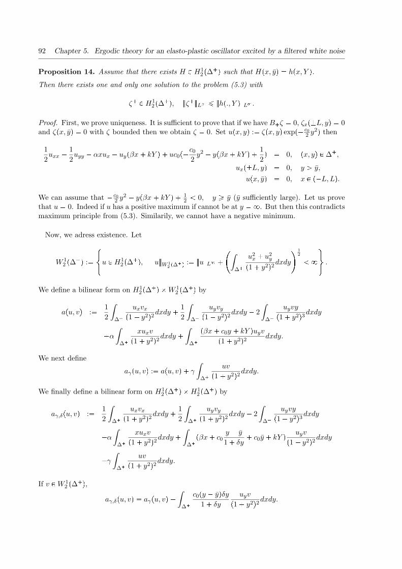
92 Chapter 5. Ergodic theory for an elasto-plastic oscillator excited by a filtered white noise
Proposition 14. Assume that there exists H P H12 ♣∆�q such that H♣x, yq ✏ h♣x, Y q.
Then there exists one and only one solution to the problem (5.3) with
ζ� P H12 ♣∆�q, ⑥ζ�⑥L✽ ↕ ⑥h♣., Y q⑥L✽ .
Proof. First, we prove uniqueness. It is sufficient to prove that if we have B�ζ ✏ 0, ζx♣✟L, yq ✏ 0and ζ♣x, yq ✏ 0 with ζ bounded then we obtain ζ ✏ 0. Set u♣x, yq :✏ ζ♣x, yq exp♣✁ c0
2y2q then
1
2uxx � 1
2uyy ✁ αxux ✁ uy♣βx� kY q � uc0♣✁c0
2y2 ✁ y♣βx� kY q � 1
2q ✏ 0, ♣x, yq P ∆�,
ux♣✟L, yq ✏ 0, y → y,
u♣x, yq ✏ 0, x P ♣✁L,Lq.
We can assume that ✁ c02y2 ✁ y♣βx � kY q � 1
2➔ 0, y ➙ y (y sufficiently large). Let us prove
that u ✏ 0. Indeed if u has a positive maximum if cannot be at y ✏ ✽. But then this contradictsmaximum principle from (5.3). Similarily, we cannot have a negative minimum.
Now, we adress existence. Let
W 12 ♣∆�q :✏
✩✫✪u P H1
2 ♣∆�q, ⑥u⑥W 12 ♣∆�q :✏ ⑥u⑥L✽ �
✄ˆ
∆�
u2x � u2
y
♣1� y2q2dxdy☛ 1
2
➔ ✽✱✳✲ .
We define a bilinear form on H12 ♣∆�q ✂W 1
2 ♣∆�q by
a♣u, vq :✏ 1
2
ˆ
∆�
uxvx
♣1� y2q2dxdy �1
2
ˆ
∆�
uyvy
♣1� y2q2dxdy ✁ 2
ˆ
∆�
uyvy
♣1� y2q3dxdy
�αˆ
∆�
xuxv
♣1� y2q2dxdy �ˆ
∆�
♣βx� c0y � kY quyv♣1� y2q2 dxdy.
We next define
aγ♣u, vq :✏ a♣u, vq � γ
ˆ
∆�
uv
♣1� y2q2dxdy.
We finally define a bilinear form on H12 ♣∆�q ✂H1
2 ♣∆�q by
aγ,δ♣u, vq :✏ 1
2
ˆ
∆�
uxvx
♣1� y2q2dxdy �1
2
ˆ
∆�
uyvy
♣1� y2q2dxdy ✁ 2
ˆ
∆�
uyvy
♣1� y2q3dxdy
�αˆ
∆�
xuxv
♣1� y2q2dxdy �ˆ
∆�♣βx� c0
y ✁ y
1� δy� c0y � kY q uyv
♣1� y2q2dxdy
�γˆ
∆�
uv
♣1� y2q2dxdy.
If v PW 12 ♣∆�q,
aγ,δ♣u, vq ✏ aγ♣u, vq ✁ˆ
∆�
c0♣y ✁ yqδy1� δy
uyv
♣1� y2q2dxdy.

5.3. The exterior Dirichlet problem 93
If u PW 12 ♣∆�q, we can compute
aγ,δ♣u, uq ✏ 1
2
ˆ
∆�
u2x
♣1� y2q2dxdy �1
2
ˆ
∆�
u2y
♣1� y2q2dxdy ✁ 2
ˆ
∆�
uyuy
♣1� y2q3dxdy
�αˆ
∆�
xuxu
♣1� y2q2dxdy �ˆ
∆�
♣βx� c0y � kY q♣1� y2q2 uyudxdy
✁c02
ˆ
∆�
u2
♣1� y2q2✒
1
1� δy✁ δ♣y ✁ yq♣1� δyq2 ✁
4♣y ✁ yqy♣1� δyq♣1� y2q
✚dxdy
�γˆ
∆�
u2
♣1� y2q2dxdy.
And see that
aγ,δ♣u, uq ➙ 1
2
ˆ
∆�
u2x
♣1� y2q2dxdy �1
2
ˆ
∆�
u2y
♣1� y2q2dxdy ✁ 2
ˆ
∆�
uyuy
♣1� y2q3dxdy
�αˆ
∆�
xuxu
♣1� y2q2dxdy �ˆ
∆�
♣βx� c0y � kY q♣1� y2q2 uyudxdy
�♣γ ✁ c0
2qˆ
∆�
u2
♣1� y2q2dxdy
and the right hand does not depend on δ. Moreover, we can define a constant γ depending onlyon the constants α, β, c0, y, k, Y but not on δ such that
aγ,δ♣v, vq ➙ a0⑥v⑥2H12 ♣∆�q, a0 → 0. (5.4)
The constant a0 depends only on α, β, c0, y, k, Y . If f♣x, yq is bounded, we consider the problem
aγ,δ♣u, v ✁ uq ➙ γ
ˆ
∆�
f♣v ✁ uq♣1� y2q2dxdy, ❅v P K, u P K (5.5)
whereK :✏ tv P H1
2 ♣∆�q, v♣x, yq ✏ h♣x, Y q✉which is not empty from the assumption. Then from the coercivity (5.4) and results of the theoryof Variational Inequalities (5.5) has one and only one solution uγδ♣fq (writing u for uγδ♣fq tosimplify notation). If w P H1
2 ♣∆�q satisfies w♣x, yq ✏ 0 then u� w P K, hence
aγ,δ♣u,wq ✏ γ
ˆ
∆�
fw
♣1� y2q2dxdy
and thus also
✁1
2uxx ✁ 1
2uyy � αxux � ♣βx� c0
y ✁ y
1� δy� c0y � kY quy � γu ✏ γf, ♣x, yq P ∆�,
ux♣✟L, yq ✏ 0, y P ♣y,�✽q,u♣x, yq ✏ h♣x, Y q, x P ♣✁L,�Lq.
Also ifMf :✏ maxt⑥h♣., Y q⑥✽, ⑥f⑥L✽✉

94 Chapter 5. Ergodic theory for an elasto-plastic oscillator excited by a filtered white noise
then⑥uγδ♣fq⑥L✽ ↕Mf .
Moreover,
aγδ♣u,H ✁ uq ➙ γ
ˆ
∆�
f♣H ✁ uq♣1� y2q2 dxdy
hence
aγδ♣u, uq ↕ aγδ♣u,Hq ✁ γ
ˆ
∆�
f♣H ✁ uq♣1� y2q2 dxdy
and
aγδ♣u,Hq ✏ aγ♣u,Hq ✁ˆ
∆�
c0♣y ✁ yqδy♣1� δyq
uyH
♣1� y2q2dxdy
↕ C⑥u⑥H12 ♣∆�q⑥H⑥W 1
2 ♣∆�q � γCMf ⑥h♣., Y q⑥✽where C depends only on constants α, β, c0y, k, Y . From (5.4), we deduce easily that
⑥uγδ♣fq⑥H12 ♣∆�q ↕ Cγ♣fq. (5.6)
Letting δ Ñ 0, we obtain
uγδ Ñ uγ♣fq in H12 ♣∆�q weakly and in L✽♣∆�q weakly-✍, uγ♣fq P K
We deduce easily from (5.5) that uγ♣fq satisfies
aγ♣u, v ✁ uq ➙ γ
ˆ
∆�
f♣v ✁ uq♣1� y2q2dxdy (5.7)
❅v PW 12 ♣∆�q, v P K, u P K, ⑥u⑥✽ ↕Mf , ⑥u⑥H1
2 ♣∆�q ↕ Cγ♣fqwhere again we write u for uγ♣fq. The solution of (5.7) is unique. Indeed, we first claim that
a♣u,wq ✏ γ
ˆ
∆�
fw
♣1� y2q2dxdy, ❅w PW 12 ♣∆�q, w♣x, yq ✏ 0.
But then if u1, u2 are two solutions
aγ♣u1, u1 ✁ u2q ✏ γ
ˆ
∆�fu1 ✁ u2
♣1� y2q2dxdy, aγ♣u2, u1 ✁ u2q ✏ γ
ˆ
∆�fu1 ✁ u2
♣1� y2q2dxdy,
hence aγ♣u1 ✁ u2, u1 ✁ u2q ✏ 0. However, from (5.4) we also have
aγ♣v, vq ➙ a0⑥v⑥2H12 ♣∆�q, ❅v P H1
2 ♣∆�q
Therefore u1 ✁ u2 ✏ 0. We next consider a sequence ζn with ζ0 ✏ ⑥h♣., Y q⑥L✽ given by thesolution of
aγ♣ζn�1, v ✁ ζn�1q ➙ γ
ˆ
∆�
ζn♣v ✁ ζn�1q♣1� y2q2 dxdy, (5.8)
where
ζn�1 P K, ❅v PW 12 ♣∆�q, v P K, ⑥ζn�1⑥L✽ ↕ max ♣⑥h♣., Y q⑥L✽ , ⑥ζn⑥L✽q .

5.3. The exterior Dirichlet problem 95
Considering ζ1, we have
aγ♣ζ1, v ✁ ζ1q ↕ γ
ˆ
∆�
ζ0♣v ✁ ζ1q♣1� y2q2 dxdy.
Take v ✏ ζ1 ✁ ♣ζ1 ✁ ζ0q�, which is admissible, then
aγ♣ζ1, ♣ζ1 ✁ ζ0q�q ↕ γ
ˆ
∆�
ζ0♣ζ1 ✁ ζ0q�♣1� y2q2 dxdy
and
aγ♣ζ1 ✁ ζ0, ♣ζ1 ✁ ζ0q�q ✏ aγ♣ζ1, ♣ζ1 ✁ ζ0q�q ✁ γ
ˆ
∆�
ζ0♣ζ1 ✁Hq�♣1� y2q2 dxdy ↕ 0
from the assumptions. Therefore ♣ζ1 ✁ ζ0q� ✏ 0 which implies ζ1 ↕ ζ0 and also
⑥ζ1⑥L✽ ↕ ⑥h♣., Y q⑥L✽ .Then by induction if ζn ↕ ζn✁1, ⑥ζn⑥L✽ ↕ ⑥h♣., Y q⑥L✽ . We obtain ζn�1 ↕ ζn, ⑥ζn�1⑥L✽ ↕⑥h♣., Y q⑥L✽ . Also
aγ♣ζn�1, ζ1 ✁ ζn�1q ➙ γ
ˆ
∆�
ζn♣ζ1 ✁ ζn�1q♣1� y2q2 dxdy
aγ♣ζn�1, ζn�1q ↕ aγ♣ζn�1, ζ1q ✁ γ
ˆ
∆�
ζn♣ζ1 ✁ ζn�1q♣1� y2q2 dxdy
↕ a♣ζn�1, ζ1q � γ
ˆ
∆�
ζ1ζn�1
♣1� y2q2dxdy ✁ γ
ˆ
∆�
ζn♣ζ1 ✁ ζn�1q♣1� y2q2 dxdy
Hence⑥ζn�1⑥H1
2 ♣∆�q ↕ Cγ
✁⑥ζ1⑥H1
2 ♣∆�q � ⑥h♣., Y q⑥✽✠.
The sequence ζn Ñ ζ is monotone decreasing and ζn Ñ ζ in H12 ♣∆�q weakly, ζ P K, ⑥ζ⑥L✽ ↕
⑥h♣., Y q⑥L✽ .Hence in the limit,
a♣ζ, v ✁ ζq ➙ 0, ❅v PW 12 ♣∆�q, v P K, ζ P K, ⑥ζ⑥L✽ ↕ ⑥h♣., Y q⑥L✽ (5.9)
and ζ is solution of equation (5.3).
The Cauchy problem
The exterior Dirichlet Problem 2 is equivalent to
Aζ ✏ 0, ♣x, y, zq P ♣✁L,Lq ✂ ♣y,✽q ✂ ♣✁Y, Y q,ζ♣x, y, zq ✏ h♣x, zq, ♣x, zq P ♣✁L,Lq ✂ ♣✁Y, Y q,ζ♣x, y, Y q ✏ ζ�♣x, yq, ♣x, yq P ♣✁L,Lq ✂ ♣y,✽q,
ζx♣✟L, y, zq ✏ 0, ♣y, zq P ♣y,✽q ✂ ♣✁Y, Y q
(5.10)
withB�ζ� ✏ 0, ♣x, yq P ♣✁L,Lq ✂ ♣y,✽q,
ζ�♣x, yq ✏ h♣x, Y q, x P ♣✁L,Lq,ζ�x ♣✟L, yq ✏ 0, y P ♣y,✽q

96 Chapter 5. Ergodic theory for an elasto-plastic oscillator excited by a filtered white noise
and⑥ζ�⑥L✽ ↕ ⑥h♣., Y q⑥L✽ .
This is a Cauchy problem, with z taking place of time and ♣x, yq as the space variable. We writeit as
ζz � 1
y
✂1
2ζyy � 1
2ζxx ✁ αxζx ✁ ♣βx� c0y � kzqζy
✡✏ 0 (5.11)
and using the notation
A♣zqu♣x, yq :✏ ✁1
y
✂1
2uyy � 1
2uxx ✁ αxux ✁ ♣βx� c0y � kzquy
✡
we obtain✁❇ζ❇z �A♣zqζ ✏ 0, ♣x, yq P ∆�, z ➔ Y,
ζ♣x, y, Y q ✏ ζ�♣x, yq, ♣x, yq P ♣✁L,Lq ✂ ♣y,✽q,ζx♣✟L, y, zq ✏ 0, ♣y, zq P ♣y,✽q ✂ ♣✁Y, Y q,ζ♣x, y, zq ✏ h♣x, zq, ♣x, zq P ♣✁L,Lq ✂ ♣✁Y, Y q.
(5.12)
So it is a Cauchy problem with mixed Dirichlet-Neuman boundary conditions. We consider thespace H1
2 ♣∆�q, with a new norm
⑥u⑥2✍ ✏ˆ
∆�
1
y
u2x � u2
y
♣1� y2q2 dxdy �ˆ
∆�
u2
♣1� y2q2 dxdy
which is not equivalent to
⑥u⑥2 ✏ˆ
∆�
u2x � u2
y
♣1� y2q2 dxdy �ˆ
∆�
u2
♣1� y2q2 dxdy.
The norm in L22♣∆�q is defined by
⑤u⑤2✍ :✏ˆ
∆�
u2
♣1� y2q2 dxdy ↕ ⑥u⑥2✍.
We define on H12 ♣∆�q the bilinear continuous form
A♣zq♣u, vq :✏ 1
2
ˆ
∆�
uxvx � uyvy
y♣1� y2q2 dxdy ✁ 1
2
ˆ
∆�
uyv♣1� 3y2qy2♣1� y2q3 dxdy
�ˆ
∆�
♣αxux � ♣βx� c0y � kzquyq vy♣1� y2q2 dxdy.
Moreover,
A♣zq♣u, uq ✏ 1
2
ˆ
∆�
u2x � u2
y
y♣1� y2q2 dxdy ✁ 1
2
ˆ
∆�
uyu♣1� 3y2qy2♣1� y2q3 dxdy
�ˆ
∆�
♣αxux � ♣βx� c0y � kzquyquy♣1� y2q2 dxdy
✁1
2
ˆ
∆�u2c0
d
dy♣ y ✁ y
y♣1� y2q2 qdxdy
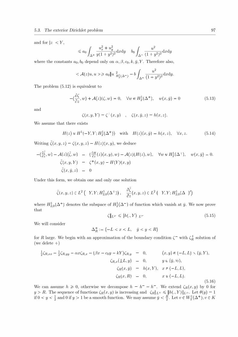
5.3. The exterior Dirichlet problem 97
and for ⑤z⑤ ➔ Y ,
↕ a0
ˆ
∆�
u2x � u2
y
y♣1� y2q2 dxdy ✁ b0
ˆ
∆�
u2
♣1� y2q2 dxdy
where the constants a0, b0 depend only on α, β, c0, k, y, Y . Therefore also,
➔ A♣zqu, u →➙ a0⑥u⑥2H12 ♣∆�q ✁ b
ˆ
∆�
u2
♣1� y2q2 dxdy.
The problem (5.12) is equivalent to
✁♣❇ζ❇z , wq �A♣zq♣ζ, wq ✏ 0, ❅w P H12 ♣∆�q, w♣x, yq ✏ 0 (5.13)
and
ζ♣x, y, Y q ✏ ζ�♣x, yq , ζ♣x, y, zq ✏ h♣x, zq.We assume that there exists
H♣zq P H1♣✁Y, Y ;H12 ♣∆�qq with H♣zq♣x, yq ✏ h♣x, zq, ❅x, z. (5.14)
Writing ζ♣x, y, zq ✏ ζ♣x, y, zq ✁H♣zq♣x, yq, we deduce
✁♣❇ζ❇z , wq �A♣zq♣ζ, wq ✏ ♣❇H❇z ♣zq♣x, yq, wq ✁A♣zq♣H♣zq, wq, ❅w P H12 ♣∆�q, w♣x, yq ✏ 0.
ζ♣x, y, Y q ✏ ζ�♣x, yq ✁H♣Y q♣x, yqζ♣x, y, zq ✏ 0
Under this form, we obtain one and only one solution
ζ♣x, y, zq P L2�✁Y, Y ;H1
2,0♣∆�q✟ , ❇ζ❇z ♣x, y, zq P L
2�✁Y, Y ;H1
2,0♣∆�q✶✟where H1
2,0♣∆�q denotes the subspace of H12 ♣∆�q of function which vanish at y. We now prove
that
⑥ζ⑥L✽ ↕ ⑥h♣., Y q⑥L✽ (5.15)
We will consider
∆�R :✏ t✁L ➔ x ➔ L, y ➔ y ➔ R✉
for R large. We begin with an approximation of the boundary condition ζ� with ζ�R solution of(we delete +)
12ζR,xx � 1
2ζR,yy ✁ αxζR,x ✁ ♣βx� c0y � kY qζR,y ✏ 0, ♣x, yq P ♣✁L,Lq ✂ ♣y, Y q,
ζR,x♣✟L, yq ✏ 0, y P ♣y,✽q,ζR♣x, yq ✏ h♣x, Y q, x P ♣✁L,Lq,ζR♣x,Rq ✏ 0, x P ♣✁L,Lq.
(5.16)We can assume h ➙ 0, otherwise we decompose h ✏ h� ✁ h✁. We extend ζR♣x, yq by 0 fory → R. The sequence of functions ζR♣x, yq is increasing and ⑥ζR⑥L✽ ↕ ⑥h♣., Y q⑥L✽ . Let θ♣yq ✏ 1if 0 ➔ y ➔ 1
2and 0 if y → 1 be a smooth function. We may assume y ➔ R
2. Let v PW 1
2 ♣∆�q, v P K

98 Chapter 5. Ergodic theory for an elasto-plastic oscillator excited by a filtered white noise
and test (5.16) withvθ♣ y
Rq✁ζR
♣1�y2q2 which vanishes at y ✏ y and y ✏ R. Setting θR♣yq ✏ θ♣ yRq, we
obtain,
1
2
ˆ
∆�R
ζR,x♣vxθR ✁ ζR,xq♣1� y2q2 dxdy � 1
2
ˆ
∆�R
ζR,y♣vyθR ✁ ζR,yq♣1� y2q2 dxdy (5.17)
� 1
2R
ˆ
∆�R
ζR,yvθ✶R
♣1� y2q2 dxdy ✁ˆ
∆�R
2ζR,y♣vθR ✁ ζRqy♣1� y2q3y dxdy
�ˆ
∆�R
αxζR♣vθR ✁ ζRq♣1� y2q2 dxdy �
ˆ
∆�R
♣βx� c0y � kY q♣1� y2q2 ζR,y♣vθR ✁ ζRqdxdy ✏ 0.
and thus also a♣ζR, vθR ✁ ζRq ✏ 0. Recalling that
a♣u, uq � γ
ˆ
∆�
u2
♣1� y2q2dxdy ➙ a0⑥u⑥2H12 ♣∆�q,
we geta0⑥ζR⑥2H1
2 ♣∆�q ↕ a♣ζR, vθRq � C⑥h♣., Y q⑥2L✽ ,from which we deduce easily,
⑥ζR⑥H12 ♣∆�q ↕ C.
We then consider the limit
ζR Ñ ζ monotone increasing , ζR Ñ ζ in H12 ♣∆�q weakly
Hence,a♣ζ, vq ↕ a♣ζ, ζq
which implies that ζ is the solution ζ� of (5.3). We next consider the approximation of (5.10)for y ➔ y ➔ R. We write
AζR ✏ 0, ♣x, yq P ∆R ✂ ♣✁Y, Y q,ζR♣x, y, Y q ✏ ζ�R ♣x, yq, ♣x, yq P ∆R,
ζR♣x, y, zq ✏ h♣x, zq, ♣x, zq P ♣✁L,Lq ✂ ♣✁Y, Y q,ζR♣x,R, zq ✏ 0, ♣x, zq P ♣✁L,Lq ✂ ♣✁Y, Y q,
ζR,x♣✟L, y, zq ✏ 0, ♣y, zq P ♣y, Rq ✂ ♣✁Y, Y q.
(5.18)
We write (5.18) as a Cauchy problem
❇ζR❇z �A♣zqζR ✏ 0, in ∆R,
ζR♣x, y,Rq ✏ ζ�R ♣x, yq, ♣x, yq P ∆�R,
ζR,x♣✟L, y, zq ✏ 0, ♣y, zq P ♣y, Rq ✂ ♣✁Y, Y q,ζR♣x, y, zq ✏ h♣x, zq, ♣x, zq P ♣✁L,Lq ✂ ♣✁Y, Y q,ζR♣x,R, zq ✏ 0, ♣x, zq P ♣✁L,Lq ✂ ♣✁Y, Y q
(5.19)
and extend ζR by 0 for y → R. If w P H12 ♣∆�q, w♣x, yq ✏ 0, we can write
✁♣❇ζR❇z , wθRq �A♣zq♣ζR, θRwq ✏ 0,
ζR♣x, y, Y q ✏ ζ�R ♣x, yq, ♣x, yq P ∆�R,
ζR♣x, y, zq ✏ h♣x, zq, ♣x, zq P ♣✁L,Lq ✂ ♣✁Y, Y q.(5.20)
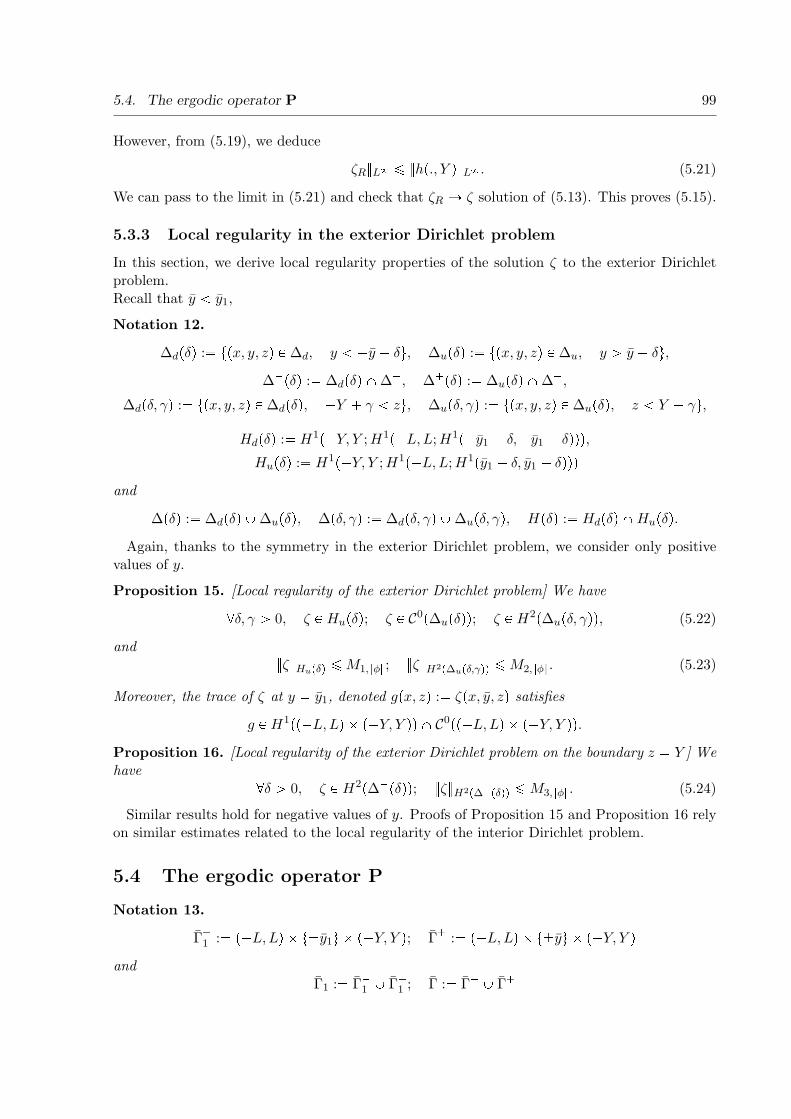
5.4. The ergodic operator P 99
However, from (5.19), we deduce
⑥ζR⑥L✽ ↕ ⑥h♣., Y q⑥L✽ . (5.21)
We can pass to the limit in (5.21) and check that ζR Ñ ζ solution of (5.13). This proves (5.15).
5.3.3 Local regularity in the exterior Dirichlet problem
In this section, we derive local regularity properties of the solution ζ to the exterior Dirichletproblem.Recall that y ➔ y1,
Notation 12.
∆d♣δq :✏ t♣x, y, zq P ∆d, y ➔ ✁y ✁ δ✉, ∆u♣δq :✏ t♣x, y, zq P ∆u, y → y � δ✉,∆✁♣δq :✏ ∆d♣δq ❳∆✁, ∆�♣δq :✏ ∆u♣δq ❳∆�,
∆d♣δ, γq :✏ t♣x, y, zq P ∆d♣δq, ✁Y � γ ➔ z✉, ∆u♣δ, γq :✏ t♣x, y, zq P ∆u♣δq, z ➔ Y ✁ γ✉,
Hd♣δq :✏ H1♣✁Y, Y ;H1♣✁L,L;H1♣✁y1 ✁ δ,✁y1 � δqqq,Hu♣δq :✏ H1♣✁Y, Y ;H1♣✁L,L;H1♣y1 ✁ δ, y1 � δqqq
and
∆♣δq :✏ ∆d♣δq ❨∆u♣δq, ∆♣δ, γq :✏ ∆d♣δ, γq ❨∆u♣δ, γq, H♣δq :✏ Hd♣δq ❳Hu♣δq.Again, thanks to the symmetry in the exterior Dirichlet problem, we consider only positive
values of y.
Proposition 15. [Local regularity of the exterior Dirichlet problem] We have
❅δ, γ → 0, ζ P Hu♣δq; ζ P C0♣∆u♣δqq; ζ P H2♣∆u♣δ, γqq, (5.22)
and⑥ζ⑥Hu♣δq ↕M1,⑥φ⑥; ⑥ζ⑥H2♣∆u♣δ,γqq ↕M2,⑥φ⑥. (5.23)
Moreover, the trace of ζ at y ✏ y1, denoted g♣x, zq :✏ ζ♣x, y, zq satisfies
g P H1♣♣✁L,Lq ✂ ♣✁Y, Y qq ❳ C0♣♣✁L,Lq ✂ ♣✁Y, Y qq.Proposition 16. [Local regularity of the exterior Dirichlet problem on the boundary z ✏ Y ] Wehave
❅δ → 0, ζ P H2♣∆�♣δqq; ⑥ζ⑥H2♣∆�♣δqq ↕M3,⑥φ⑥. (5.24)
Similar results hold for negative values of y. Proofs of Proposition 15 and Proposition 16 relyon similar estimates related to the local regularity of the interior Dirichlet problem.
5.4 The ergodic operator P
Notation 13.
Γ✟1 :✏ ♣✁L,Lq ✂ t✟y1✉ ✂ ♣✁Y, Y q; Γ✟ :✏ ♣✁L,Lq ✂ t✟y✉ ✂ ♣✁Y, Y qand
Γ1 :✏ Γ✁1 ❨ Γ�1 ; Γ :✏ Γ✁ ❨ Γ�

100 Chapter 5. Ergodic theory for an elasto-plastic oscillator excited by a filtered white noise
5.4.1 Construction of the operator P
Consider φ :✏ ♣φ✁, φ�q P L✽♣Γ1q. Following the same procedure of the 1d case, we first solvethe interior Dirichlet problem for η with the boundary condition✩✫
✪η ✏ φ� in Γ�1 ,
η ✏ φ✁ in Γ✁1 .
Then
⑥η⑥L✽ ↕ max♣⑥φ�⑥, ⑥φ✁⑥q.Then, we solve the exterior Dirichlet problem for ζ with the boundary condition✩✫
✪ζ ✏ η in Γ�,
ζ ✏ η in Γ✁.
Then
⑥ζ⑥L✽ ↕ ⑥η⑥L✽ ↕ ⑥φ⑥L✽ .For p1 P Γ1, let us define
Pφ♣p1q :✏ ζ♣p1q.
5.4.2 Probabilistic interpretation of the operator P
Let us recall from Khasminskii [27] the probabilistic interpretation of the operator P. For p P Γand for p1 P Γ1, we denote by γ1♣p; .q the distribution of z♣τ1q starting from p and by γ♣p1; .qthe distribution of z♣τq starting from p1. We showed
η♣pq ✏ˆ
Γ1
φ♣uqγ1♣p; duq and ζ♣p1q ✏ˆ
Γ
η♣vqγ♣p1; dvq.
Also, using Fubini theorem we can write
Pφ♣p1q ✏ˆ
Γ1
φ♣uqγγ1♣p1, duq,
where
γγ1♣p1, duq :✏ˆ
Γ
γ♣p1; dvqγ1♣v; duq.
By construction, the operator P is the transition probability associated to the Markov chain
t♣x♣τ1,kq, y♣τ1,kq, z♣τ1,kqq✉k➙0
where τ1,0 ✏ 0 and
τk�1 :✏ inftt → τ1,k, ⑤y♣tq⑤ ✏ y✉; τ1,k�1 :✏ inftt → τk�1, ⑤y♣tq⑤ ✏ y1✉.
Note that τk�1 ✏ τ ✆ θτ1,kand τ1,k�1 ✏ τ1 ✆ θτk�1
where θt is the shift operator.

5.4. The ergodic operator P 101
5.4.3 Ergodic property for P
Theorem 5.4.1. The operator P is ergodic.
Proof. A Borel subset of Γ1 can be written as B :✏ B✁ ✂ ty1✉ ❨ B� ✂ t✁y1✉ with B�, B✁ areBorel subsets of ♣✁L,Lq ✂ ♣✁Y, Y q. We have
B� ✏ t♣x, zq : ♣x, y1, zq P B✉ and B✁ ✏ t♣x, zq : ♣x,✁y1, zq P B✉
also
1B�♣x, zq ✏ 1B♣x, y1, zq; 1B✁♣x, zq ✏ 1B♣x,✁y1, zq.Consider φ� ✏ 1B� and φ✁ ✏ 1B✁ in the interior Dirichlet problem, then
P♣1Bq♣x, y, zq ✏✩✫✪
ζ♣x, y1, zq if y ✏ y1
ζ♣x,✁y1, zq if y ✏ ✁y1.
Let p, p P Γ1, define
λp,p♣Bq :✏ P♣1Bq♣pq ✁P♣1Bq♣pq.We will prove the ergodic property of the operator P in the four following steps.
1. Doob’s criterion from [17].The operateur P is ergodic if we prove the following Doob’s criterion
supλp,p♣Bq ➔ 1, ❅p, p P Γ1 and ❅B.
2. Negation of Doob’s criterion.Suppose Doob’s criterion is not verified. Then, there exists two sequences pk :✏ ♣xk, yk, zkq,pk :✏ ♣xk, yk, zkq in Γ1 and a sequence of Borel subset Bk such that
λpk,pk♣Bkq Ñ 1.
Denote ηk and ζk the solution of the interior and exterior Dirichlet problems with φ� ✏1B�k
and φ✁ ✏ 1B✁k, where B�k and B✁k are deduced from Bk as previously. We have
λpk,pk♣Bkq ✏ ζk♣xk, yk, zkq ✁ ζk♣xk, yk, zkq.
Now, extracting a subsequence of pk and pk, we deduce
pk Ñ p✍ and pk Ñ p✍ in Γ1.
Also,
p✍ ✏ ♣x✍, y1, z✍q or ♣x✍,✁y1, z
✍qand
p✍ ✏ ♣x✍, y1, z✍q or ♣x✍,✁y1, z
✍q.From (5.22), we know that
⑥ζk⑥H♣δq ↕M1,1 and ⑥ζk⑥H2♣∆♣δ,γqq ↕M2,1

102 Chapter 5. Ergodic theory for an elasto-plastic oscillator excited by a filtered white noise
then
ζk P H♣δq ⑨ C0♣∆♣δqq,ζk Ñ ζ✍ in H♣δq weakly,
ζ✍ P C0♣∆♣δqq,and
ζk Ñ ζ✍ in C0♣∆♣δ, γqq.
(5.1)
From (5.23), we know that
⑥ζk⑥H2♣∆✟♣δqq ↕M3,1,
so, we obtain
ζk Ñ ζ✍ in C0♣∆✟♣δqq. (5.2)
Proposition 17. Under the hypothesis that P is not ergodic, we have ζ✍♣p✍q ✏ 1.
Proof. We must have limkÑ✽ ζk♣pkq ✏ 1.
(a) If ⑤z✍⑤ ➔ Y or z✍y✍ ✏ ✁Y y1 then (5.1) implies limkÑ✽ ζk♣pkq ✏ ζ✍♣p✍q.(b) If z✍y✍ ✏ Y y1 then (5.2) implies limkÑ✽ ζk♣xk,✟y1,✟Y q ✏ ζ✍♣p✍q. Indeed, as for all
k ➙ 0, ζk is continuous, there exists σk ➙ k such that ⑤ζk♣pσkq ✁ ζk♣xσk
,✟y1,✟Y q⑤ ↕2✁k. Also, limkÑ✽ ζk♣pσk
q ✏ limkÑ✽ ζk♣xσk,✟y1,✟Y q ✏ ζ✍♣p✍q.
3. Contradiction.Suppose p✍ ✏ ♣x✍, y1, z
✍q and set
Ξ1 :✏ Γ1 ❳ tx ✏ ✟L✉; Ξ2 :✏ Γ1 ❳ tz ✏ Y ✉.
Maximum principle for parabolic operator applied to ζ✝ implies p✍ P Ξ1 ❨ Ξ2. Then p✍
cannot be in Ξ1 because of the Neuman condition and p✍ cannot be in Ξ2 because ofthe boundary condition z ✏ Y . A similar argument yields a contradiction with p✍ ✏♣x✍,✁y1, z
✍q.
4. Conclusion.From ergodic theory, there exists a unique probability mesure γ✍ ✏ ♣γ✁✍ , γ�✍ q on Γ1 andK, ρ → 0 such that
❅n ➙ 0,
✞✞✞✞✞Pnφ✁¨
Γ✁1φ♣r, sqdγ✁✍ ♣r, sq ✁
¨
Γ�1φ♣r, sqdγ�✍ ♣r, sq
✞✞✞✞✞ ↕ K⑥φ⑥ exp♣✁ρnq. (5.3)

5.5. The nonhomogeneous interior Dirichlet problem 103
5.5 The nonhomogeneous interior Dirichlet problem
Consider f a bounded function on ∆1, we want to define E♣x,y,zq�´ τ10f♣x♣sq, y♣sq, z♣sqqds✟ as
the solution of the non-homogeneous interior Dirichlet Problem 3:
Statement of the problem 3. Find χ P L✽♣∆1q ❳ C0♣∆ǫ1q,❅ǫ → 0 such that
Aχ� f ✏ 0 in ∆1,
B✟χ� f ✏ 0 in ∆✟1 ,
χ♣x,✟y1, zq ✏ 0 in ♣✁L,Lq ✂ ♣✁Y, Y q,χx♣✟L, y, zq ✏ 0 in ♣✁y1, y1q ✂ ♣✁Y, Y q.
ConsiderΦ♣x, y, zq :✏ expλ♣c0kz2 � c0y
2q; λ ➙ 1.
Theorem 5.5.1. The Problem 3 has a unique solution. Moreover, we have
⑥χ⑥L✽ ↕ expλ♣c0kY 2 � c0y21q,
where λ depends on f .
Proof. The uniqueness of a solution of Problem 3 is argued as the uniqueness for the homoge-neous Dirichlet interior problem. The existence can be proven by the regularization techniqueused previously. Now, we give a L✽ bound for χ. We have
φx ✏ 0; φxx ✏ 0
φy ✏ 2yc0λφ; φyy ✏ 2c0λφ� ♣2c0λyq2φφz ✏ 2zc0kλφ
and
yφz ✁ αxφx ✁ φy♣βx� c0y � kzq � 1
2φyy � 1
2φxx ✏ ✁2βc0λxyφ✁ 2c20λy
2φ� c0λφ� 2♣c0λyq2
✏ c0λφ✁ c0λ2βxyφ� 2♣c0yq2λ♣λ✁ 1qφ➙ c0λ♣1✁ 2βLy1qφ� 2♣c0yq2λ♣λ✁ 1qφ➙ ⑥f⑥
where y1 can be chosen as 2y1 ➔ 12βL
, and λ ➙ max♣1, ⑥f⑥c0♣1✁2βLy1qq.
Using that φ♣x, y,✟Y q ✏ expλ♣c0kY 2q expλ♣c20y2q we obtain for z ✏ Y, 0 ➔ y ➔ y1.
✁αxφx ✁ φy♣βx� c0y � kY q � 1
2φyy � 1
2φxx ✏ ✁φy♣x, y, Y q♣c0y � kY � βxq � 1
2φyy♣x, y, Y q
✏ λc0φ♣x, y, Y q�1✁ 2♣kY � βxqy � 2c0♣λ✁ 1qy2
✟➙ λc0φ♣x, y, Y q
�1✁ 2♣kY � βLqy � 2c0♣λ✁ 1qy2
✟➙ λc0
�1✁ ♣kY � βLq2
2c0♣λ✁ 1q✟
➙ ⑥f⑥,

104 Chapter 5. Ergodic theory for an elasto-plastic oscillator excited by a filtered white noise
if λ ➙ max♣2 ⑥f⑥c0, 1 � ♣kY�βLq2
c0q. Similar estimates hold for z ✏ ✁Y,✁y1 ➔ y ➔ 0. Consider
u :✏ φ✁ χ, then u satisfies the following inequalities
Au ➙ 0 in ∆1; B✟u ➙ 0 in ∆✟1 (5.1)
and the following boundary conditions
u♣x,✟y1, zq ✏ exp♣λ�c0kz2 � c0y21
✟q in ♣✁L,Lq ✂ ♣✁Y, Y q,ux♣✟L, y, zq ✏ 0 in ♣✁y1, y1q ✂ ♣✁Y, Y q. (5.2)
The maximum of u cannot be attained in ∆1 or on the boundaries z ✏ ✟Y, x ✏ ✟L. It can onlybe attained for y ✏ y1 or y ✏ y1. Hence,
u♣x, y, zq ↕ exp♣λ♣c0kY 2 � c0y21qq
which impliesχ♣x, y, zq ➙ ✁ exp♣λ♣c0kY 2 � c0y
21qq.
Now, consider v ✏ ✁♣φ� χq, then v satisfies inequalities (5.3)
Av ↕ 0 in ∆1; B✟v ↕ 0 in ∆✟1 (5.3)
and the boundary condition (5.4)
v♣x,✟y1, zq ✏ ✁ exp♣λ�c0kz2 � c0y21
✟q in ♣✁L,Lq ✂ ♣✁Y, Y q,vx♣✟L, y, zq ✏ 0 in ♣✁y1, y1q ✂ ♣✁Y, Y q. (5.4)
Again, the minimum of v cannot be attained in ∆1 or on the boundaries z ✏ ✟Y, x ✏ ✟L.Hence
v♣x, y, zq ➙ ✁ exp♣λ♣c0kY 2 � c0y21qq
which impliesχ♣x, y, zq ↕ exp♣λ♣c0kY 2 � c0y
21qq.
Now, let us derive some estimates on derivatives. Let M :✏ exp♣λ♣c0kY 2 � c0y12qq. Using the
test function m0♣x, y, zq ✏ exp♣✁c0♣y2 � kz2qq exp♣✁αx2q we obtain now a priori estimates onthe partial derivatives of χ. We test (3) with m0χˆ
∆1
χ2ym0 �
ˆ
∆1
χ2xm0 ✏
ˆ
❇∆1,z✏Yyχ2m0 ✁
ˆ
❇∆1,z✏✁Yyχ2m0 � 2
ˆ
∆1
fχm0 ✁ˆ
∆1
c0βxχ2m0
↕ˆ
❇∆1,z✏Y,y→0
yχ2m0 ✁ˆ
❇∆1,z✏✁Y,y➔0
yχ2m0 � 2
ˆ
∆1
fχ
↕ C♣Mq.Hence,
ˆ
∆1
χ2ym0 ↕ C♣Mq ;
ˆ
∆1
χ2xm0 ↕ C♣Mq.
We have then,ˆ
∆1
♣y2χzq2m0 ↕ C♣Mq and
ˆ
∆1
♣y2χyyq2m0 ↕ C♣Mq.
The function χ is smooth outside a neighborhood of y ✏ 0.

5.6. The nonhomogeneous exterior Dirichlet problem 105
5.6 The nonhomogeneous exterior Dirichlet problem
Consider the function
Ψ♣yq :✏ log♣yq �K, K such that log♣y1q �K → 0
and the space of functionsX✽
Ψ :✏ tuψ, u P L✽♣∆uq✉.We want to define E♣x,y,zq
�´ τ
0f♣x♣sq, y♣sq, z♣sqqds✟ as the solution of the nonhomogeneous ex-
terior Dirichlet Problem 4:
Statement of the problem 4. Find ξ P X✽Ψ ❳ C0♣∆ǫ
uq,❅ǫ → 0 such as
Aξ � f ✏ 0 in ∆u,
B�ξ � f ✏ 0 in ∆�,
ξ♣x, y, zq ✏ 0 in ♣✁L,Lq ✂ ♣✁Y, Y q,ξx♣✟L, y, zq ✏ 0 in ♣y,�✽q ✂ ♣✁Y, Y q.
Theorem 5.6.1. The Problem 4 has a unique solution. Moreover, we have ✁ψ♣yq ↕ ξ♣x, y, zq ↕ψ♣yq.Proof. We justify uniqueness of the solution taking f ✏ 0 and setting ξ
ξ ✏ wψα, α → 1.
We show w ✏ 0. In particular, w satisfies
ξ ✏ wψα
ξx ✏ wxψα; ξy ✏ wyψ
α � wαψyψα✁1; ξz ✏ wzψ
α
ξxx ✏ wxxψα; ξyy ✏ wyyψ
α � 2wyαψyψα✁1 � wα
�ψyyψ
α✁1 � ♣ψyq2ψα✁2♣α✁ 1q✟
then
1
2wxxψ
α � 1
2twyyψα � 2wyαψyψ
α✁1wα�ψyyψ
α✁1 � ♣ψyq2ψα✁2♣α✁ 1q✉✁♣c0y � kz � βxqtwyψα � wαψyψ
α✁1✉ ✁ αxwxψα � ywzψ
α ✏ 0.
Collecting terms related to ψα, we obtain
1
2wxx � 1
2twyy � 2wyα
ψy
ψ� wα
�ψyyψ
� ♣ψyq2ψ2
♣α✁ 1q✉
�♣✁c0y ✁ kz ✁ βxqtwy � wαψy
ψ✉ ✁ αxwx � ywz ✏ 0,
which implies for z P ♣✁Y, Y q and y → y,
1
2wxx � 1
2wyy � wytαψy
ψ✁ c0 ✁ kz ✁ βx✉ � wα
ψt12ψyy � ♣α✁ 1q
2
♣ψyq2ψ
✁♣c0y � kz � βxqαψy✉ ✁ αxwx � ywz ✏ 0

106 Chapter 5. Ergodic theory for an elasto-plastic oscillator excited by a filtered white noise
and for z ✏ Y ; y → y,
1
2wxx � 1
2wyy � wytαψy
ψ✁ c0 ✁ kY ✁ βx✉ � wα
ψt12ψyy � ♣α✁ 1q
2
♣ψyq2ψ
✁ ♣c0y � kY � βxqαψy✉ ✁ αxwx � ywz ✏ 0
andw♣x, y, zq ✏ 0.
We can find α → 1 with α✁ 1 small so that
1
2ψyy ✁ ♣c0y � kz � βxq � ♣α✁ 1q♣ψyq
2
ψ↕ ✁γ c0
2� ♣α✁ 1qγy2♣log♣yq �Kq ➔ 0.
Since w Ñ 0 as y Ñ ✽, a positive maximum can be attained only for a finite y✍. But this isimpossible from the equation. So w is negative,w ↕ 0. But, w is also positive, w ➙ 0. Henceξ ✏ 0 and uniqueness follows.Now, existence is demonstrated by the following approximation
AξR � f ✏ 0, in ∆R,
B�ξR � f ✏ 0, in ∆�R,
ξ♣x, y, zq ✏ 0, ξ♣x,R, zq ✏ 0,
ξx♣✟L, y, zq ✏ 0.
Using uR ✏ ξR ✁ ψ, we obtainAuR ➙ 0, in ∆R,
B�uR ➙ 0, in ∆�R,
uR♣x, y, zq ✏ ✁ψ♣yq,uRx ♣✟L, y, zq ✏ 0.
Necessarily, uR ↕ 0. The sequence ξR is monotone increasing and converges towards a solution.Let us show estimates on u. Suppose f ➙ 0, we will show that 0 ↕ ξ ↕ ψ. Then,
ψy♣✁c0y ✁ kz ✁ βxq � 1
2ψyy ✏ γr1
y♣✁c0y ✁ kz ✁ βxq ✁ 1
2y2s
↕ γr1y♣✁c0y ✁ kzq ✁ 1
2y2s
↕ γr1y♣✁c0y ✁ kzq ✁ 1
2y2s
↕ ✁γ c02, if y → 2kY
c0.
Define γ such that γc02➙ ⑥f⑥. We then have, setting u ✏ ξ ✁ ψ,
Au ➙ 0, in ∆
B�u ➙ 0, in ∆�
u♣x, y, zq ✏ ✁ψ♣yqux♣✟L, y, zq ✏ 0

5.7. The operator T and the invariant measure ν 107
It follows that u ↕ 0.We can show similarly that ξ � φ ➙ 0. Hence, we have
✁ψ ↕ ξ ↕ ψ.
5.7 The operator T and the invariant measure ν
5.7.1 Construction of the operator T
Consider f P L✽♣Oq, following the same procedure of the 1d case, we first solve the interior non-homogeneous Dirichlet problem for χ with f at the right hand side, then we solve the exteriornon-homogeneous Dirichlet problem for ξ with f at the right hand side and χ as a boundarycondition. Also, for any p1 P Γ1, we define the operator
Tf♣p1q :✏ ξ♣p1q.
This defines a linear operator from L✽�Γ1
✟in L✽♣Γ1q.
5.7.2 Probabilistic interpretation of the operator T
For any A a Borel subset of O, consider the two following measures of occupation of A by theprocess ♣x♣tq, y♣tq, z♣tqq starting at p P O, namely
★νχ♣p;Aq :✏ Ep
�´ τ10
1A♣x♣sq, y♣sq, z♣sqqds✟
νξ♣p;Aq :✏ Ep
�´ τ
01A♣x♣sq, y♣sq, z♣sqqds
✟.
We have shown
χ♣pq ✏ˆ
O
f♣qqdνχ♣p; dqq and ξ♣pq ✏ˆ
O
f♣qqdνξ♣p; dqq.
For any p1 P Γ1, we have
T♣fq♣p1q :✏ Ep1
�ˆ τ1
0
f♣x♣sq, y♣sq, z♣sqqds✟� ˆΓ
Eq
�ˆ τ
0
f♣x♣sq, y♣sq, z♣sqqds✟dγ♣p1; dqq
T♣fq integrates f over a time cycle of the Markov chain stopped on Γ1, that is ♣x♣τ1,kq, y♣τ1,kq, z♣τ1,kqq.
5.7.3 Construction of the invariant measure ν
Now, define
ν♣fq :✏´ L
✁L´ Y
✁Y Tf♣r, y1, sqγ�✍ ♣dr, dsq �´ L
✁L´ Y
✁Y Tf♣r,✁y1, sqγ✁✍ ♣dr,dsq´ L
✁L´ Y
✁Y T1♣r, y1, sqγ�✍ ♣dr,dsq �´ L
✁L´ Y
✁Y T1♣r,✁y1, sqγ✁✍ ♣dr,dsq.
The denominator is well defined and is stricly positive. Now, we want to solve the complete problem.

108 Chapter 5. Ergodic theory for an elasto-plastic oscillator excited by a filtered white noise
Statement of the problem 5. Find u such that uψ✁1 is bounded for ⑤y⑤ → ⑤y⑤ and
Au� f ✏ 0, in O
B�u� f ✏ 0, in O�
B✁u� f ✏ 0, in O✁
ux♣✟L, y, zq ✏ 0, in tx ✏ ✟L✉ ❳O
Considering Problems 1, 2, 3 and 4, in the following result we use a functional analysis methodto prove that ν is the unique invariant distribution associated to the solution ♣x♣tq, y♣tq, z♣tqq ofthe stochastic variational inequality (5.2).
Theorem 5.7.1. The Problem 5 has a unique solution if and only if ν♣fq ✏ 0.
Proof. Similar arguments as the 1d case are considered. Uniqueness is guaranteed by the ergodicproperty of the operator P. Suppose ν♣fq ✏ 0. We define χ the solution of the Interior non-homogeneous Dirichlet Problem 3 and ξ the solution of the Exterior non-homogeneous DirichletProblem 4. We set χ0 :✏ χ and ξ0 :✏ ξ, and for k ➙ 0, we define χk�1 by
Aχk�1 ✏ 0, in ∆1,
B�χk�1 ✏ 0, in ∆�1 ,
B✁χk�1 ✏ 0, in ∆✁1 ,
χk�1x ♣✟L, y, zq ✏ 0, in ♣✁y1, y1q ✂ ♣✁Y, Y q
with
χk�1♣x, y1, zq ✏ ξk♣x, y1, zq; χk�1♣x,✁y1, zq ✏ ξk♣x,✁y1, zq.Afterwards, we define ξk�1 by
Aξk�1 ✏ 0, in ∆u,
B�ξk�1 ✏ 0, in ∆�u ,
ξk�1x ♣✟L, y, zq ✏ 0, in ♣y,�✽q ✂ ♣✁Y, Y q
with
ξk�1♣x, y, zq ✏ χk�1♣x, y, zq.Similarly, we define ξk�1 by
Aξk�1 ✏ 0, in ∆d,
B✁ξk�1 ✏ 0, in ∆✁d ,
ξk�1x ♣✟L, y, zq ✏ 0, in ♣✁✽,✁yq ✂ ♣✁Y, Y q
with
ξk�1♣x,✁y, zq ✏ χk�1♣x,✁y, zq.That means
ξ0⑤Γ1✏ Tf ; ξk�1⑤Γ1
✏ P♣ξk⑤Γ1q.

5.7. The operator T and the invariant measure ν 109
Next, we setξk ✏ ξ0 � ξ1 � ...� ξk; χk ✏ χ0 � χ1 � ...� χk
thenξk⑤Γ1
✏ Tf �P♣Tfq � ...�Pk♣Tfq.Now, let us remark that χk satisfies the following equation:
Aχk � f ✏ 0, in ∆1,
B�χk � f ✏ 0, in ∆�1 ,
B✁χk � f ✏ 0, in ∆✁1 ,
χkx♣✟L, y, zq ✏ 0, in ♣✁✽,✁yq ✂ ♣✁Y, Y q
(5.1)
withχk♣x, y1, zq ✏ ξk✁1♣x, y1, zq; χk♣x,✁y1, zq ✏ ξk✁1♣x,✁y1, zq
ξk satisfies the following equations:
Aξk � f ✏ 0, in ∆u,
B�ξk � f ✏ 0, in ∆�u ,
ξkx♣✟L, y, zq ✏ 0, in ♣y,�✽q ✂ ♣✁Y, Y q(5.2)
ξk♣x, y, zq ✏ χk♣x, y, zqand
Aξk � f ✏ 0, in ∆d,
B�ξk � f ✏ 0, in ∆✁d ,
ξkx♣✟L, y, zq ✏ 0, in ♣✁✽,✁yq ✂ ♣✁Y, Y q(5.3)
ξk♣x,✁y, zq ✏ χk♣x,✁y, zq.The condition ν♣fq ✏ 0 means
ˆ
Γ1
Tf♣xqdπ♣xq ✏ˆ
Γ1
Tf♣r,✁y1, sqdπ1♣r, sq �ˆ
Γ1
Tf♣r, y1, sqdπ2♣r, sq ✏ 0.
From the estimate (5.3), we obtained
ξk converges in L✽♣Γ1q.
Now, we notice that χk ✁ χ is a solution of the interior homogeneous Dirichlet problem with♣χk ✁ χq⑤Γ1
✏ ξk✁1⑤Γ1and ξk ✁ ξ is a solution of the Exterior homogeneous Dirichlet problem
with ♣ξk ✁ ξq⑤Γ ✏ ♣χk ✁ χq⑤Γ. Then, we obtain
⑥ξk ✁ ξ⑥L✽ ↕ ⑥χk ✁ χ⑥L✽ ↕ ⑥ξk✁1⑥L✽ ↕ C.
We can extract a subsequence such that
ξk Ñ ξ; χk Ñ χ.
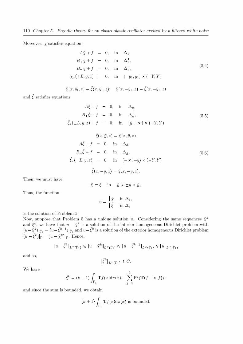
110 Chapter 5. Ergodic theory for an elasto-plastic oscillator excited by a filtered white noise
Moreover, χ satisfies equation:
Aχ� f ✏ 0, in ∆1,
B�χ� f ✏ 0, in ∆�1 ,
B✁χ� f ✏ 0, in ∆✁1 ,
χx♣✟L, y, zq ✏ 0, in ♣✁y1, y1q ✂ ♣✁Y, Y q
(5.4)
χ♣x, y1, zq ✏ ξ♣x, y1, zq; χ♣x,✁y1, zq ✏ ξ♣x,✁y1, zqand ξ satisfies equations:
Aξ � f ✏ 0, in ∆u,
B�ξ � f ✏ 0, in ∆�u ,
ξx♣✟L, y, zq � f ✏ 0, in ♣y,�✽q ✂ ♣✁Y, Y q(5.5)
ξ♣x, y, zq ✏ χ♣x, y, zqAξ � f ✏ 0, in ∆d,
B✁ξ � f ✏ 0, in ∆✁d ,
ξx♣✟L, y, zq ✏ 0, in ♣✁✽,✁yq ✂ ♣✁Y, Y q(5.6)
ξ♣x,✁y, zq ✏ χ♣x,✁y, zq.Then, we must have
χ ✏ ξ in y ➔ ✟y ➔ y1
Thus, the function
u ✏★χ in ∆1,
ξ in ∆c1
is the solution of Problem 5.Now, suppose that Problem 5 has a unique solution u. Considering the same sequences χk
and ξk, we have that u ✁ χk is a solution of the interior homogeneous Dirichlet problem with♣u✁χkq⑤Γ1
✏ ♣u✁ ξk✁1q⑤Γ1and u✁ ξk is a solution of the exterior homogeneous Dirichlet problem
♣u✁ ξkq⑤Γ ✏ ♣u✁ χkq⑤Γ. Hence,
⑥u✁ ξk⑥L✽♣Γ1q ↕ ⑥u✁ χk⑥L✽♣Γ1q ↕ ⑥u✁ ξk✁1⑥L✽♣Γ1q ↕ ⑥u⑥L✽♣Γ1q
and so,⑥ξk⑥L✽♣Γ1q ↕ C.
We have
ξk ✏ ♣k � 1qˆ
Γ1
Tf♣xqdπ♣xq �k➳j✏0
Pj♣T♣f ✁ ν♣fqqq
and since the sum is bounded, we obtain
♣k � 1qˆ
Γ1
Tf♣xqdπ♣xq is bounded.

5.7. The operator T and the invariant measure ν 111
That leads toˆ
Γ1
Tf♣xqdπ♣xq ✏ 0
That implies ν♣fq ✏ 0.
Consider now ϕ a smooth function in r✁L,Ls✂R✂r✁Y, Y s with compact support. If we take
f ✏ ✁Aϕ,f♣x, y, Y q ✏ ✁B�ϕ,f♣x, y,✁Y q ✏ ✁B✁ϕ,
then ϕ is solution of (5) for this f . From Theorem 5.7.1, we have
´ L
✁L´✽✁✽´ Y
✁Y✥1
2ϕyy � 1
2ϕxx ✁ αxϕx ✁ ♣βx� c0y � kzqϕy � yϕz
✭dν♣x, y, zq
� ´ L
✁L´✽0
✥1
2ϕyy � 1
2ϕxx ✁ αxϕx ✁ ♣βx� c0y � kY qϕy
✭dν♣x, y, Y q
� ´ L
✁L´ 0
✁✽✥1
2ϕyy � 1
2ϕxx ✁ αxϕx ✁ ♣βx� c0y ✁ kY qϕy
✭dν♣x, y,✁Y q ✏ 0.
If ν has a density m, then we deduce that
α❇❇x rxms�
❇❇y r♣βx� c0y�kzqms✁ y
❇m❇z � 1
2
❇2m
❇x2� 1
2
❇2m
❇y2✏ 0 in ♣0, Lq✂R✂♣✁Y, Y q (5.7)
in the sense of distributions. If we test (5.7) with ϕ and integrate by parts, we obtain
✁ˆ L
✁L
ˆ �✽
✁✽ym♣x, y, Y qϕ♣x, y, Y qdxdy �
ˆ L
0
ˆ �✽
✁✽ym♣x, y,✁Y qϕ♣x, y,✁Y qdxdy
�ˆ L
✁L
ˆ ✽
✁✽
ˆ Y
✁Ym♣x, y, zq✥1
2ϕyy � 1
2ϕxx ✁ αxϕx ✁ ♣βx� c0y � kzqϕy � yϕz
✭dxdydz ✏ 0
and comparing with (5.7)
✁ˆ L
✁L
ˆ 0
✁✽ym♣x, y, Y qϕ♣x, y, Y qdxdy �
ˆ L
0
ˆ �✽
0
ym♣x, y,✁Y qϕ♣x, y,✁Y qdxdy
✁ˆ L
✁L
ˆ ✽
0
m♣x, y, Y q✥1
2ϕyy � 1
2ϕxx ✁ αxϕx ✁ ♣βx� c0y � kY qϕy � yϕ
✭dxdy
✁ˆ L
✁L
ˆ 0
✁✽m♣x, y,✁Y q✥1
2ϕyy � 1
2ϕxx ✁ αxϕx ✁ ♣βx� c0y ✁ kY qϕy ✁ yϕ
✭dxdy ✏ 0
we finally deduce
ym� ❇❇x rxms �
❇❇y r♣βx� c0y � kY qms � 1
2
❇2m
❇x2� 1
2
❇2m
❇y2✏ 0, on O�
✁ym� ❇❇x rxms �
❇❇y r♣βx� c0y ✁ kY qms � 1
2
❇2m
❇x2� 1
2
❇2m
❇y2✏ 0, on O✁
m ✏ 0, on ♣✁L,Lq ✂ ♣✁✽, 0q ✂ tY ✉ ❨ ♣✁L,Lq ✂ ♣0,✽q ✂ t✁Y ✉The proof of the main result is complete.

112 Chapter 5. Ergodic theory for an elasto-plastic oscillator excited by a filtered white noise
5.8 Appendix: Proofs of lemmas 5,6,7,8
Proof of Lemma 5. Denote γ ✏ ⑥φ⑥L✽ . Notice we have
♣u✁ γq�♣x,✟y1, zq ✏ 0 if x P ♣✁L,Lq, z P ♣✁Y, Y q♣u✁ γq�♣x, y,✟Y q ✏ 0 if x P ♣✁L,Lq, 0 ➔ ✟y ➔ y1
and
♣u� γq✁♣x,✟y1, zq ✏ 0 if x P ♣✁L,Lq, z P ♣✁Y, Y q♣u� γq✁♣x, y,✟Y q ✏ 0 if x P ♣✁L,Lq, 0 ➔ ✟y ➔ y1.
Choose v ✏ u✁ ♣u✁ γq� P K and we obtain
✁a♣u, ♣u✁ γq�q ✁ λ♣u, ♣u✁ γq�q ➙ ✁λ♣w, ♣u✁ γq�q
a♣u, ♣u✁ γq�q � λ♣u, ♣u✁ γq�q ↕ λ♣w, ♣u✁ γq�q.
Switching the first argument by ♣u✁ γq in the previous inequality, we obtain
a♣♣u✁ γq�, ♣u✁ γq�q � λ⑤♣u✁ γq�⑤2L2 ↕ λ♣w ✁ γ, ♣u✁ γq�q
and w ↕ γ implies ♣u✁ γq� ✏ 0. Taking v ✏ u� ♣u� γq✁ similar arguments yields ♣u� γq✁ ✏0.
Proof of Lemma 6. We have the following expressions,
a♣ηǫ, ηǫq ✏ˆ
∆1
ǫ
2♣ηǫzq2 �
1
2♣ηǫyq2 �
1
2♣ηǫxq2 � ♣βx� kz � c0yqηǫηǫy ✁ yηǫηǫz � αxηǫηǫx
and
a♣ηǫ, u0q ✏ˆ
∆1
ǫ
2ηǫzu0z � 1
2ηǫyu0y � 1
2ηǫxu0x � ♣βx� kz � c0yqu0η
ǫy ✁ yu0η
ǫz � αxu0η
ǫx.
Inequality a♣ηǫ, ηǫq ↕ a♣ηǫ, u0q means
ǫ
2
ˆ
∆1
♣ηǫzq2 �1
2
ˆ
∆1
♣ηǫxq2 �1
2
ˆ
∆1
♣ηǫyq2 ↕ǫ
2
ˆ
∆1
ηǫzu0z � 1
2
ˆ
∆1
ηǫyu0y
✁ˆ
∆1
♣βx� c0y � kzqηǫηǫy �1
2
ˆ
∆1
♣βx� c0y � kzqu0ηǫy
�1
2
ˆ
∆1
ηǫxu0x �ˆ
∆1
αxηǫηǫx ✁ˆ
∆1
αxu0ηǫx
�ˆ
∆1
yηǫηǫz ✁ˆ
∆1
yu0ηǫz
We apply Cauchy-Schwartz inequality to the first two terms, then we apply Green formula to

5.8. Appendix: Proofs of lemmas 5,6,7,8 113
the last one and we get
ǫ
2
ˆ
∆1
♣ηǫzq2 �1
2
ˆ
∆1
♣ηǫxq2 �1
2
ˆ
∆1
♣ηǫyq2 ↕ ǫ
❞ˆ
∆1
♣ηǫzq21
2♣ˆ
∆1
♣uǫ0zq2q12
�❞ˆ
∆1
♣ηǫyq2t1
2♣ˆ
∆1
♣uǫ0yq2q12 � ⑥φ⑥♣
ˆ
∆1
♣βx� c0y � kzq2q 12 ✉
�❞ˆ
∆1
♣ηǫxq2t1
2♣ˆ
∆1
♣uǫ0xq2q12 � α⑥φ⑥♣
ˆ
∆1
x2q 12 � α♣
ˆ
∆1
x2u0q12 ✉
�⑥φ⑥2ˆ L
✁L
ˆ y1
✁y1⑤y⑤dxdy � ⑥φ⑥♣
ˆ
∆1
⑤yu0z⑤q �ˆ L
✁L
ˆ y1
✁y1⑤y⑤⑤u0♣x, y, Y q⑤
�ˆ L
✁L
ˆ y1
✁y1⑤y⑤⑤u0♣x, y,✁Y q⑤
with c1,c2,c3 and c4 are positive constant, we get
⑥❄ǫηǫz⑥2L2 � ⑥ηǫy⑥2L2 � ⑥ηǫx⑥2L2 ↕❄ǫc1⑥
❄ǫηǫz⑥L2 � c2⑥ηǫy⑥L2 � c3⑥ηǫx⑥L2 � c4.
Proof of Lemma 7. We have
ˆ
∆1
ηkyyηkzy
2p✁1θ2q ✏ ✁ˆ
∆1
ηkyηkzyy
2p✁1θ2q ✁ˆ
∆1
ηkyηkz ♣2p✁ 1qy2p✁2θ2q ✁
ˆ
∆1
ηkyηkzy
2p✁12qθ✶θ2q✁1
✏ ✁1
2
ˆ
∆1
♣♣ηky q2qzy2p✁1θ2q ✁ ♣2p✁ 1qˆ
∆1
♣ηkyθq♣ηkzy2p✁2θ2q✁1q
✁ 2q
ˆ
∆1
♣ηkyθq♣ηkzy2p✁1θ2q✁2qθ✶
✏ ✁1
2
ˆ L
✁L
ˆ y1
✁y1♣ηky q2♣x, y, Y qy2p✁1θ2q � 1
2
ˆ L
✁L
ˆ y1
✁y1♣ηky q2♣x, y,✁Y qy2p✁1θ2q
✁ ♣2p✁ 1qˆ
∆1
♣ηkyθq♣ηkzπqyp✁2θq✁1 ✁ 2q
ˆ
∆1
♣ηkyθq♣ηkzπqyp✁1θq✁2θ✶,
ˆ
∆1
ηkxxηkzy
2p✁1θ2q ✏ ✁1
2
ˆ
∆1
♣♣ηkxq2qzy2p✁1θ2q
✏ ✁1
2
ˆ L
✁L
ˆ y1
✁y1♣ηkxq2♣x, y, Y qy2p✁1θ2q � 1
2
ˆ L
✁L
ˆ y1
✁y1♣ηkxq2♣x, y,✁Y qy2p✁1θ2q
andˆ
∆1
♣c0y � kz � βxqηkyηkzy2p✁1θ2q ✏ˆ
∆1
♣c0y � kz � βxq♣ηkyθq♣ηkzπqyp✁1θq✁1
ˆ
∆1
αxηkxηkzy
2p✁1θ2q ✏ˆ
∆1
αx♣ηkxθq♣ηkzπqyp✁1θq.

114 Chapter 5. Ergodic theory for an elasto-plastic oscillator excited by a filtered white noise
Testing ♣Aηkq with ηkzy2p✁1θ2q, we deduce
ˆ
♣ηkzπq2 ✏ 1
4
ˆ L
✁L
ˆ y1
✁y1♣ηky q2♣x, y, Y qy2p✁1θ2q ✁ 1
4
ˆ L
✁L
ˆ y1
✁y1♣ηky q2♣x, y,✁Y qy2p✁1θ2q
�1
4
ˆ L
✁L
ˆ y1
✁y1♣ηkxq2♣x, y, Y qy2p✁1θ2q ✁ 1
4
ˆ L
✁L
ˆ y1
✁y1♣ηkxq2♣x, y,✁Y qy2p✁1θ2q
�♣p✁ 1
2qˆ
∆1
♣ηkyθq♣ηkzπqyp✁2θq✁1 � q
ˆ
∆1
♣ηkyθq♣ηkzπqyp✁1θq✁2θ✶
�ˆ
∆1
♣c0y � kz � βxq♣ηkyθq♣ηkzπqyp✁1θq✁1
�ˆ
∆1
αx♣ηkxθq♣ηkzπqyp✁1θq.
Proof of Lemma 8. 1. With
f♣ηk, ηky q :✏ ✁ηk♣π✷
2✁ ♣c0y � kz � αxqπ✶q ✁ ηkyπ
✶,
we have ❅ψ P H1♣∆1q, ψ♣x, y,✟Y q ✏ 0 and ψ♣x,✟y1, zq ✏ 0,
1
2
ˆ
∆1
vkyψy �1
2
ˆ
∆1
vkxψx �ˆ
∆1
�αxvkx � ♣βx� c0y � kzqvky ✁ yvkz
✟ψ ✏
ˆ
∆1
f♣ηk, ηky qψ.
Now, when k goes to �✽, we get
1
2
ˆ
∆1
vyψy � 1
2
ˆ
∆1
vxψx �ˆ
∆1
�αxvx � ♣βx� c0y � kzqvy ✁ yvz
✟ψ ✏
ˆ
∆1
f♣η, ηyqψ.
We deduce that in H✁1♣∆1q we firstly have ✁Av ✏ f♣η, ηyq which is equivalent to πAη ✏ 0
and secondly that choice of test function implies πηx♣✟L, y, zq ✏ 0 in ♣H 12 ♣♣✁L,Lq ✂
♣✁y1, y1qq✶.
2. (a) We know that πηk P H1♣∆1q, its trace is well defined and satisfies,
γ♣πηkq♣x, y, Y q ✏ π♣χ�,k � βk,�q; y → 0
γ♣πηkq♣x, y,✁Y q ✏ πχ✁,k; y ➔ 0
with
⑥χ✟,k⑥L✽ ↕ ⑥φ⑥L✽ (5.8)
and χ✁,k, χ�,k satisfy respectively (5.9) and (5.10)
´ L
✁L´ y10t1
2♣χ�,kx ψx � χ
�,ky ψyq � ♣αxχ�,kx � ♣βx� c0y � kY qχ�,ky qψ✉dxdy ✏ 0,
❅ψ P H1♣♣✁L,Lq ✂ ♣0, y1qq with ψ♣x, 0q ✏ ψ♣x, y1q ✏ 0
(5.9)

5.8. Appendix: Proofs of lemmas 5,6,7,8 115
and
´ L
✁L´ 0
✁y1t12♣χ✁,kx ψx � χ
✁,ky ψyq � ♣αxχ✁,kx � ♣βx� c0y ✁ kY qχ✁,ky qψ✉dxdy ✏ 0,
❅ψ P H1♣♣✁L,Lq ✂ ♣✁y1, 0qq with ψ♣x, 0q ✏ ψ♣x,✁y1q ✏ 0.
(5.10)First, we study convergence of the sequence χ✟,k and we deduce PDEs satisfied bylimkÑ0 χ
✟,k.In particular (5.8) implies
χ�,k Ñ χ� in L2♣♣✁L,Lq ✂ ♣0, y1qq weakly,
χ✁,k Ñ χ✁ in L2♣♣✁L,Lq ✂ ♣✁y1, 0qq weakly.
and equalities (5.9), (5.10) imply
⑥χ�,kπ⑥H1 ↕ C and χ�,kπ Ñ χ�π in H1♣♣✁L,Lq ✂ ♣0, y1qq weakly,
⑥χ✁,kπ⑥H1 ↕ C and χ✁,kπ Ñ χ✁π in H1♣♣✁L,Lq ✂ ♣✁y1, 0qq weakly.
Denote ξ✟,k :✏ χ✟,ky2 and g♣χ�,k, χ�,ky q :✏ ✁χ�,kt1✁ 2y♣αx� c0y � kY q✉ ✁ 2yχ�,ky .
From (5.9), we have BY ξ�,k ✏ g♣χ�,k, χ�,ky q in ♣✁L,Lq✂♣✁y1, y1q, in H✁1♣♣✁L,Lq✂
♣0, y1qq. The operator B� is strictly elliptic then ξ�,k P H2♣♣✁L,Lq ✂ ♣0, y1qq. We
have ξ�,kx ♣✟L, yq ✏ 0 in ♣H 12 ♣0, y1qq✶. As ξ�,k P H2♣∆1q and πB�χ�,k ✏ 0, we have
✁B�ξ�,k ✏ g♣χ�,k, χ�,ky q in a strong sense
We obtain that ❅ψ P H1♣♣✁L,Lq ✂ ♣0, y1qq, ψ♣x, 0q ✏ ψ♣x, y1q ✏ 0,
ˆ L
✁L
ˆ y1
0
1
2♣ξ�,kx ψx � ξ�,ky ψyq �
�αxξ�,kx � ♣βx� c0y � kY qξ�,ky ✁ yξ�,kz
✟ψ
✏ˆ L
✁L
ˆ y1
0
g♣χk, χkyqψ.
Now, when k goes to 0, we have
ˆ L
✁L
ˆ y1
0
1
2♣ξ�x ψx�ξ�y ψyq�
�αxξ�x �♣βx�c0y�kY qξ�y ✁yξ�z
✟ψ ✏
ˆ L
✁L
ˆ y1
0
g♣χ, χyqψ.
We deduce that in H✁1♣♣✁L,Lq ✂ ♣0, y1qq we have ✁B�ξ� ✏ g♣χ�, χ�y q which isequivalent to y2B�χ� ✏ 0 and that choice of test function implies y2χ�x ♣✟L, yq ✏ 0
in ♣H 12 ♣♣0, y1qqq✶.
(b) Firstly, γ♣πηkq Ñ π♣χ� � β�q in H1♣♣✁L,Lq ✂ ♣0, y1qq weakly. Secondly, weak con-vergence of πηk Ñ πη in H1♣∆1q implies weak convergence of γ♣πηkq Ñ γ♣πηq in
H12 ♣❇∆1q. By uniqueness of the limit, we have γ♣πηq ✏ π♣χ� � β�q.
3. Using Green formula
❅ψ P H10 ♣∆1q ❳H2♣∆1q,
ˆ
∆1
ηkψyy �ˆ
∆1
ηkyψy ✏ˆ
❇∆1
φkψydσ.

116 Chapter 5. Ergodic theory for an elasto-plastic oscillator excited by a filtered white noise
Now, when k goes to ✽, we obtain
❅ψ P H10 ♣∆1q ❳H2♣∆1q,
ˆ
∆1
ηψyy �ˆ
∆1
ηyψy ✏ˆ
❇∆1
φψydσ.
Lemma 9. We have
ηxxπ2 P L2♣∆1q; ηxyπ
2 P L2♣∆1q; ηyyπ2 P L2♣∆1q
Proof. Denote w :✏ vx. Deriving equation (5.30) with respect to x, we obtain equality (5.11),
✁1
2wxx ✁ 1
2wyy � Λ♣x, y, zqwy � αxwx ✁ ywz ✏ ✁βvy ✁ αvx � ρ1ηx � ♣ρ1qxη � ρ2♣yqηxy (5.11)
Testing equality (5.11) with π2, we obtain
1
2
ˆ
∆1
♣wxπq2 � 1
2
ˆ
∆1
♣wyπq2 ✏ ✁ˆ
∆1
wyππ✶w ✁
ˆ
∆1
Λ♣x, y, zqwywπ2 ✁ˆ
∆1
αxwxwπ2
�ˆ
∆1
ywzwπ2 ✁ β
ˆ
∆1
vywπ2 ✁ α
ˆ
∆1
vxwπ2 �ˆ
∆1
ρ1ηxwπ2
�ˆ
∆1
♣ρ1qxηwπ2 �ˆ
∆1
ηxyρ2♣yqwπ2
which means
1
2
ˆ
∆1
♣wxπq2 � 1
2
ˆ
∆1
♣wyπq2 ✏ ✁ˆ
∆1
wyππ✶w ✁
ˆ
∆1
Λ♣x, y, zqwywπ2 ✁ˆ
∆1
αxwxwπ2
�ˆ
❇∆1
yπ2w2~n♣zqdσ ✁ β
ˆ
∆1
vywπ2 ✁ α
ˆ
∆1
vxwπ2
�ˆ
∆1
ρ1w2π �
ˆ
∆1
♣ρ1qxηwπ2 �ˆ
∆1
ηxyρ2♣yqwπ2
�ˆ
∆1
♣wyπqρ2♣yqw ✁ˆ
∆1
vxπ✶ρ2♣yqw.
It is easy to verify that vxxπ, vxyπ P L2♣∆1q.Denote w :✏ vy. Deriving equation (5.30), with respect to x, we obtain equality (5.12),
✁1
2wxx✁1
2wyy�c0w�Λ♣x, y, zqwy�αxwx✁ywz ✏ vz�ρ1ηy�♣ρ1qyη�ηyyρ2♣yq�ηyρ2♣yq✶. (5.12)
Then, we test equality (5.12) with π2w, we obtain
1
2
ˆ
∆1
♣wxπq2 � 1
2
ˆ
∆1
♣wyπq2 ✏ ✁ˆ
∆1
wyππ✶w ✁
ˆ
∆1
c0♣wπq2 ✁ˆ
∆1
Λ♣x, y, zqwywπ2 ✁ˆ
∆1
αxwxwπ2
�ˆ
∆1
vzwπ2 �ˆ
∆1
ywzwπ2 �ˆ
∆1
ηyρ1wπ2 �ˆ
∆1
η♣ρ1qywπ2
�ˆ
∆1
ηyyρ2wπ2 �ˆ
∆1
ηy♣ρ2q✶π2w

5.8. Appendix: Proofs of lemmas 5,6,7,8 117
which means
1
2
ˆ
∆1
♣wxπq2 � 1
2
ˆ
∆1
♣wyπq2 ✏ ✁ˆ
∆1
wyππ✶w ✁
ˆ
∆1
c0♣wπq2 ✁ˆ
∆1
Λ♣x, y, zqwywπ2
✁ˆ
∆1
αxwxwπ2 �ˆ
∆1
vzwπ2 �ˆ
❇∆1
y♣wπq2~n♣zqdσ �ˆ
∆1
ηyρ1wπ2
�ˆ
∆1
η♣ρ1qywπ2 �ˆ
∆1
♣wy ✁ 2ηyπ✶ � ηπ✷qwπ �
ˆ
∆1
ηy♣ρ2q✶π2w.
Again, it is easy to verify that vyxπ, vyyπ P L2♣∆1q.
Lemma 10. We have
ηxzy2π4 P L2♣∆1q; ηyzy
2π3 P L2♣∆1q.
Proof. We test equality (5.11) with y2p✁1π2qwz, we obtain
✁1
2
ˆ
wxx♣y2p✁1π2qwzq ✏ 1
2
ˆ
∆1
wxwzxy2p✁1π2q
✏ 1
4
¨
w2x♣x, y, Y qy2p✁1π2qdxdy ✁ 1
4
¨
w2x♣x, y,✁Y qy2p✁1π2qdxdy
✁1
2
ˆ
∆1
wyy♣y2p✁1π2qwzq ✏ 1
2
ˆ
∆1
wywzyy2p✁1π2q �
ˆ
∆1
wywz�♣2p✁ 1qy2p✁2π2q � y2p✁12qπ2q✁1π✶
✟✏ 1
4
¨
w2y♣x, y, Y qy2p✁1π2qdxdy ✁ 1
4
¨
w2y♣x, y,✁Y qy2p✁1π2qdxdy
� ♣p✁ 1
2qˆ
∆1
♣wyπq♣wzypπqq♣yp✁2πq✁1q � q
ˆ
∆1
♣wyπq♣wzypπqq♣yp✁1πq✁1π✶q.
We have
ˆ
∆1
♣ypπqwzq2 ↕ 1
4
¨
tw2x♣x, y, Y q � w2
y♣x, y, Y q✉y2p✁1π2qdxdy
✁ 1
4
¨
tw2x♣x, y,✁Y q � w2
y♣x, y,✁Y q✉y2p✁1π2qdxdy
� ♣p✁ 1
2qˆ
∆1
♣wyπq♣wzypπqq♣yp✁2πq✁1q � q
ˆ
∆1
♣wyπq♣wzypπqq♣yp✁1πq✁2π✶q
�ˆ
∆1
Λ♣x, y, zq♣wyπq♣wzypπqqyp✁1πq✁1 �ˆ
∆1
αx♣wxπq♣wzypπqqyp✁1πq✁1
�ˆ
∆1
βvy♣ypπqwzqyp✁1πq �ˆ
∆1
αvx♣ypπqwzqyp✁1πq
✁ˆ
∆1
ρ1vx♣ypπqwzqyp✁1πq✁1 �ˆ
∆1
♣ρ1qxη♣ypπqwzqyp✁1πq
✁ˆ
∆1
ρ2♣vxyπ ✁ vxπ✶q♣ypπqwzqyp✁1πq✁3.
For p ➙ 2 and q ➙ 3, some calculations give vxzy2π3 P L2♣∆1q.

118 Chapter 5. Ergodic theory for an elasto-plastic oscillator excited by a filtered white noise
Now, we test equality (5.12) with y2p✁1π2qwz, we obtain
ˆ
∆1
♣ypπqwzq2 ↕ 1
4
¨
tw2x♣x, y, Y q � w2
y♣x, y, Y q✉y2p✁1π2qdxdy
✁ 1
4
¨
tw2x♣x, y,✁Y q � w2
y♣x, y,✁Y q✉y2p✁1π2qdxdy
� ♣p✁ 1
2qˆ
∆1
♣wyπq♣wzypπqq♣yp✁2πq✁1q � q
ˆ
∆1
♣wyπq♣wzypπqq♣yp✁1πq✁2π✶q
�ˆ
∆1
c0w♣ypπqwzqyp✁1πq
�ˆ
∆1
Λ♣x, y, zq♣wyπq♣wzypπqqyp✁1πq✁1 �ˆ
∆1
αx♣wxπq♣wzypπqqyp✁1πq✁1
✁ˆ
∆1
vz♣ypπqwzqyp✁1πq ✁ˆ
∆1
ρ1♣vy ✁ ηπ✶q♣ypπqwzqyp✁1πq✁1
✁ˆ
∆1
♣ρ1qyη♣ypπqwzqyp✁1πq ✁ˆ
∆1
♣ρ1qxη♣ypπqwzqyp✁1πq.
✁ˆ
∆1
ρ2♣yqηyyπ2♣ypπqwzqyp✁1πq✁2
For p ➙ 2 and q ➙ 2, some calculations gives vyzy2π2 P L2♣∆1q.
Lemma 11. For p and q large enough, we have
ηxyzypπq P L2♣∆1q; ηyyzy
pπq P L2♣∆1q; ρ♣zqηxxzypπq P L2♣∆1q; ρ♣zqηzzypπq P L2♣∆1q.

Appendix A
An empirical study on plastic
deformations of an elasto-plastic
problem with noise
Ce chapitre fait l’objet d’un article soumis a Probabilistic Engineering Mechanics, [21] en col-laboration avec Cyril Feau.
Statistical properties of the plastic deformation related to an elastic per-fectly plastic oscillator under standard white noise excitation are studied inthis paper. Our approach relies on a stochastic variational inequality gov-erning the evolution between the velocity and the non-linear restoring force.Bensoussan-Turi have shown that the solution is an ergodic Markov pro-cess. In this work, we investigate elastic phasing by means of the invariantmeasure. First, we exhibit by probabilistic simulations the phenomenon ofmicro-elastic phases (small as well as numerous). The main difficulty re-lated to micro-elastic phasing is that they interfere on quantities of interestsuch that frequency of plastic deformations which tends to be overestimated.Therefore, we present approximations of the probability density function limitof the elastic component and a similar expression to Rice’s formula related tofrequency of threshold crossings. Then, these quantities are solution of partialdifferential equations. Numerical experiments on these equations show thatthe non-linear restoring force tends to be highly distributed in the neighbor-hood of plastic thresholds. Finally, an interesting criterion is provided whichcould be useful in engineering problems to discard micro-elastic phases andto evaluate statistics of plastic deformations.
Introduction
In this paper statistics of a deformation problem are investigated in the case of a non-linearstructure excited by a random process. The behavior of an elastic-perfectly-plastic (EPP) oscil-lator subjected to zero mean Gaussian white noise excitation is considered. This is the simpleststructural model exhibiting a behavior with hysteresis.
119

120 Appendix A. An empirical study on plastic deformations
Moreover, the model is simple and representative of the behavior of mechanical structures whichvibrate mainly on their first mode of deformation. In the context of earthquake engineering,relevant applications to piping systems under random vibrations can be accessed in this way[19, 20].The main difficulty to study these systems comes from a frequent occurrence of non-linear phases(plastic phases) on small intervals of time. One non-linear phase corresponds to a permanentdeformation, or in other words a plastic deformation. A plastic deformation is produced whenthe stress of the structure crosses over an elastic limit. The dynamics of the EPP-oscillator hasmemory, so it has been formulated in the engineering literature as a process with hysteresis.Denoting x♣tq the displacement and y♣tq :✏ ✾x♣tq the velocity of the oscillator, we study theproblem
✾y � c0y � F♣x♣sq, 0 ↕ s ↕ tq ✏ ✾w, (A.1)
with initial conditions of displacement and velocity
x♣0q ✏ x , y♣0q ✏ y.
Here c0 → 0 is the viscous damping coefficient, k → 0 the stiffness, w is a Wiener processand F♣tx♣sq, 0 ↕ s ↕ t✉q is a non-linear functional which depends on the entire trajectorytx♣sq, 0 ↕ s ↕ t✉ up to time t. The process of plastic deformation is denoted by ∆♣tq at time tand can be deduced from the pair ♣x♣tq,F♣x♣sq, 0 ↕ s ↕ tqq. Throughout this paper, we shallconsider the following EPP-restoring force
F♣tx♣sq, 0 ↕ s ↕ t✉q ✏✩✫✪
kY, if x♣tq ✏ Y �∆♣tq,k♣x♣tq ✁∆♣tqq, if x♣tq Ps ✁ Y �∆♣tq, Y �∆♣tqr,
✁kY, if x♣tq ✏ ✁Y �∆♣tq,(A.2)
where Y is the elastic-plastic limit. Karnopp & Scharton [26] proposed to separate elastic andplastic states by introducing a fictitious variable z♣tq :✏ x♣tq ✁ ∆♣tq. Indeed, they noticed thesimple fact, that between two plastic phases, z♣tq behaves like a linear oscillator. Therefore, x♣tqis splitted into x♣tq ✏ z♣tq�∆♣tq where z♣tq (respectively ∆♣tq) is the elastic component (respec-tively plastic) of x♣tq. So, the process ♣y♣tq, z♣tqq is relevant for engineers because estimation ofstatistics related to the deformations can be obtained.
Basically, one plastic deformation begins when z♣tq reaches and is absorbed by Y (resp. ✁Y )with positive (resp. negative) slope, y♣tq → 0. (resp. y♣tq ➔ 0) i.e. when sign♣y♣tqqz♣tq ✏ Y .Then, the plastic behavior ends when the velocity changes sign. At this moment, the elasticbehavior is reactivated. However, the velocity which is subjected to white noise, changes signan infinite number of times during any small time interval. Often, this leads to a return intoplastic behavior in a short time duration. We refer this phenomenon as micro-elastic phasing(unknown so far) which plays a crucial role on frequency and statistics of plastic deformations.Because of this phenomenon, frequency of occurrence, statistics (time duration or absolute plas-tic deformation) and the sequence of entry in plastic phase (as well as the sequence of exit) arenot well defined.
In this paper, we introduce enlarged plastic phases because we are interested in propertiesof the plastic behavior during intervals of time delimited by entries in plastic phases and bycrossings by z♣tq of the threshold Y ✁ ǫ (resp. ✁Y � ǫ) with a negative (resp. positive) velocityfor a small ǫ → 0.

121
This approach allows to rigorously link the number of enlarged plastic phases to the numberof times z♣tq crosses the threshold ✟Y ✠ ǫ with negative or positive slope.
To explain the procedure, consider T → 0, denote τ ǫ0 :✏ 0 and
θǫn�1 :✏ inftt → τ ǫn, ⑤z♣tq⑤ ✏ Y ✉,τ ǫn�1 :✏ inftt → θǫn�1, ⑤z♣tq⑤ ✏ Y ✁ ǫ✉, ❅n ➙ 1. (A.3)
Also, we set N ǫT ✏ ➦n➙0 1tτǫ
n↕T ✉ the number of enlarged plastic phases up to the time T .Then, for any measurable function f such that f♣y, zq ✏ 0 if sign♣yqz ✘ Y and satisfying´
D� ⑤f♣y, Y q⑤m♣y, Y qdy �´
D✁ ⑤f♣y,✁Y q⑤m♣y,✁Y qdy ➔ ✽, we have
1
T
ˆ T
0
f♣y♣sq, z♣sqqds ✏ N ǫT
T✂ 1
N ǫT
NǫT➳
n✏1
ˆ τǫn
θǫn
f♣y♣sq, z♣sqqds. (A.4)
So we can define separately, the frequency of crossings by z♣tq of both thresholds ✟Y ✠ ǫ withnegative or positive slope by
ν♣Y, ǫq :✏ limTÑ✽
N ǫT
T
and the “empirical statistics” related to the enlarged plastic phase by
∆f ♣Y, ǫq :✏ limTÑ✽
1
N ǫT
NǫT➳
n✏1
ˆ τǫn
θǫn
f♣y♣sq, z♣sqqds.
The asymptotic behavior of the EPP-oscillator has been studied by Bensoussan and Turi in [7].They have shown that ♣y♣tq, z♣tqq satisfies a stochastic variational inequality (SVI) and is anergodic Markov process. Thus, there exists a unique invariant measure also denoted by m♣y, zqwhich is composed of
1. an elastic part: tm♣y, zq, ⑤z⑤ ➔ Y ✉,2. a positive plastic part: tm♣y, Y q, y → 0✉,3. a negative plastic part: tm♣y,✁Y q, y ➔ 0✉.
Therefore, as T goes to infinity, (A.4) becomes
ˆ ✽
0
f♣y, Y qm♣y, Y qdy �ˆ 0
✁✽f♣y,✁Y qm♣y,✁Y qdy ✏ ν♣Y, ǫq∆f ♣Y, ǫq. (A.5)
The above relation is essential since that states that the product of ν♣Y, ǫq and ∆f ♣Y, ǫq remainsconstant for all values of ǫ. However, in our probabilistic simulations, we observe that ν♣Y, ǫqtends to ✽ and ∆f ♣Y, ǫq tends to 0 as ǫ tends to 0. In this work, we provide an empiricalcriterion which could be useful for engineers to calibrate ǫ in order to compute a frequency andstatistics of plastic deformations which does not take into account the micro-elastic phasing.Indeed, we discovered empirically that a high concentration at the neighborhood of tz ✏ ✟Y ✉can be observed in the distribution of limtÑ✽ z♣tq. Thus, the latter admits points of minimawhich are identified, namely ✟♣Y ✁ ǫ✍q. Our approach relies on partial differential equations(PDEs) related to the second marginal of tm♣y, zq, ⑤z⑤ ➔ Y ✉, that is sÑ ´✽✁✽m♣y, sqdy.

122 Appendix A. An empirical study on plastic deformations
In addition, mean frequencies of crossing thresholds✟♣Y ✁ǫ✍q with negative or positive velocityare successfully computed by an expression similar to Rice’s formula [31]. This is a techniquewidely used among engineers and is rigorously established for purely elastic systems. Moreprecisely, if Y ✏ �✽ there is no plastic deformation, z♣tq ✏ x♣tq and (A.1) reduces to thedynamics response of a linear oscillator excited by a white noise excitation. It is described bythe pair ♣x♣tq, y♣tqq which is solution of the Stochastic Differential Equation (SDE):
dy♣tq ✏ ✁♣c0y♣tq � kx♣tqqdt� dw♣tq; dx♣tq ✏ y♣tqdt. (A.6)
The couple ♣x♣tq, y♣tqq is an ergodic Markov process whose invariant measure m is explicitlygiven by [30]:
m♣x, yq ✏ c0❄k
πexp♣✁c0kx2q exp♣✁c0y2q. (A.7)
Consider s, mean frequencies ν✟s of threshold crossings with positive slope y♣tq → 0 or negativeslope y♣tq ➔ 0 are given by Rice’s formula [31]:
ν�s ✏ˆ �✽
0
ym♣y, sqdy, ν✁s ✏ ✁ˆ 0
✁✽ym♣y, sqdy. (A.8)
In the context of the EPP-oscillator ♣Y ➔ ✽q, the analogy of Rice’s formula for the calculationof ν♣Y, ǫq leads to the following approximation
ν♣Y, ǫq ✓ ✁ˆ 0
✁✽ym♣y, Y ✁ ǫqdy �
ˆ �✽
0
ym♣y,✁Y � ǫqdy. (A.9)
The proof of “Rice’s formula” for m is still an open problem and unfortunately we do not answerto this question. But, numerical experiments on tm♣y, zq, ⑤z⑤ ➔ Y ✉ to compute ν♣Y, ǫq haveprovided satisfactory results in good agreement with the probabilistic algorithm.
Organization of the paper
Section 1 is devoted to setting the governing SVI of the pair ♣y♣tq, z♣tqq. As we are interestedin the long time behavior, we seek the asymptotic law of ♣y♣tq, z♣tqq which corresponds to itsinvariant measure. The latter is solution of a PDE. The numerical method developed in [3] tosolve this PDE is also briefly summarized.In Section 2, we investigate elastic phasing. We exhibit the phenomenon of micro-elastic phaseswhich are also small as well as numerous. Micro-elastic phases are observable on numericalsolution of SVI and the frequency of switching regime in (A.3) increases significantly as ǫ tendsto 0. On the other hand, a high concentration at the neighborhood of tz ✏ ✟Y ✉ can be ob-served in the probability density function (pdf) of limtÑ✽ z♣tq. Thus, the latter admits pointsof minima which are identified. Therefore, points of inflection of the derivatives of the pdf oflimtÑ✽ z♣tq are located using approximations of PDEs. To the best of our knowledge, there isno known numerical probabilistic algorithm that does the same. These points constitute appro-priate thresholds s� ✏ Y ✁ ǫ✍ and s✁ ✏ ✁Y � ǫ✍ related to our procedure. Indeed, ǫ✍ appearsto be an interesting choice to calibrate ǫ in (A.5).In Section 3, we study applications of “Rice’s formula” to m♣y, zq. For some values of Y , we ob-serve that a similar expression to Rice’s formula is empirically valid for thresholds s ✏ s✁, s� byusing approximations of formula (A.9). Hence, in both cases, the mean frequencies of thresholdcrossings are deduced from solutions of PDEs. Of interest to engineering problems, an expressionof this frequency which does not take into account the elastic excursions is given. Moreover inthis context, statistics of plastic displacements are provided such as time duration and expectedabsolute deformation.

A.1. Some Background 123
A.1 Some Background
In [7], A. Bensoussan and J. Turi showed the dynamics of EPP-oscillator (A.1),(A.2) follows astochastic variational inequality:✩✬✬✫
✬✬✪dy♣tq ✏ ✁♣c0y♣tq � kz♣tqqdt� dw♣tq,♣dz♣tq ✁ y♣tqdtq♣ζ ✁ z♣tqq ➙ 0,
❅ ⑤ζ⑤ ↕ Y, ⑤z♣tq⑤ ↕ Y.
(A.10)
A general framework dealing with this class of inequalities can be found in [2]. For an initialcondition ♣y♣0q, z♣0qq with a given law of probability, the system is well established. In [7]existence, uniqueness and ergodicity are proven. Hence, there exists a unique invariant measurerelated to the process ♣y♣tq, z♣tqq.
A.1.1 Direct numerical simulations
In Appendix, we recall how a semi analytical solution of (A.10) has been obtained in [3]. FigureA.1 shows (a) the sojourns in the elastic and plastic phases, (b) the sojourns in micro-elasticand micro-plastic phases.
A.1.2 Characterization of the invariant measure
Notation 14. Introduce
D :✏ R✂ ♣✁Y,�Y q, D� :✏ ♣0,✽q ✂ tY ✉, D✁ :✏ ♣✁✽, 0q ✂ t✁Y ✉, (A.11)
and the differential operators
Au :✏ ✁1
2uyy � ♣c0y � kzquy ✁ yuz, (A.12)
B�u :✏ ✁1
2uyy � ♣c0y � kY quy,
B✁u :✏ ✁1
2uyy � ♣c0y ✁ kY quy,
where u is a regular function on D.
By definition, the invariant measure of the process ♣y♣tq, z♣tqq denoted by ν satisfies
ˆ
D
Aϕdν♣y, zq �ˆ ✽
0
B�ϕdν♣y, Y q �ˆ 0
✁✽B✁ϕdν♣y,✁Y q ✏ 0 , ❅ϕ regular.
The measure ν has a pdf denoted by m. Then, m satisfies by nature a PDE in an ultra weakvariational sense:
ˆ �✽
✁✽
ˆ Y
✁Ym♣y, zqty❇zϕ✁ ♣c0y � kzq❇yϕ� 1
2❇yyϕ✉dydz �
ˆ �✽
0
m♣y, Y qt✁♣c0y � kY q❇yϕ♣y, Y q � 1
2❇yyϕ♣y, Y q✉dy �
ˆ 0
✁✽m♣y,✁Y qt✁♣c0y ✁ kY q❇yϕ♣y,✁Y q � 1
2❇yyϕ♣y,✁Y q✉dy ✏ 0. (A.13)

124 Appendix A. An empirical study on plastic deformations
0 5 10 15 20 25 30 35 40 45 50−1
−0.8
−0.6
−0.4
−0.2
0
0.2
0.4
0.6
0.8
1
c0 = 1, k = 1, Y = 1
z(t)
t
µ−elastic excursions
−2.5 −2 −1.5 −1 −0.5 0 0.5 1 1.5 2 2.5−1
−0.8
−0.6
−0.4
−0.2
0
0.2
0.4
0.6
0.8
1
c0 = 1, k = 1, Y = 1
z(t)
y(t)
31 31.5 32 32.5 33 33.5 34 34.5 35 35.5 360.86
0.88
0.9
0.92
0.94
0.96
0.98
1
1.02
c0 = 1, k = 1, Y = 1
z(t)
t−1 −0.5 0 0.5 1 1.5
0.86
0.88
0.9
0.92
0.94
0.96
0.98
1
1.02
c0 = 1, k = 1, Y = 1
z(t)
y(t)
Figure A.1: Visualization of Micro-Elastic Phasing Phenomenon: At the top-left we have sampletrajectory of ♣t, z♣tqq, at the top-right we have the corresponding trajectory ♣y♣tq, z♣tqq in the phasespace; we observe regular elastic and plastic phasing. At the bottom in the both cases, a zoomon plastic phasing reveals an illustrative micro-elastic phasing.
In [3], a deterministic method alternative to the Monte Carlo method has been developed forsolving numerically (A.13). The method is compatible with the ultra weak variational formula-tion. The key point is to solve a stationary PDE with a measurable function f , satisfying
ˆ
D
⑤f♣y, zq⑤m♣y, zqdydz �ˆ
D�⑤f♣y, Y q⑤m♣y, Y qdy �
ˆ
D✁⑤f♣y,✁Y q⑤m♣y,✁Y qdy ➔ ✽, (A.14)
as right hand side: ✩✫✪
λu�Au ✏ f♣y, zq in D,
λu�B�u ✏ f♣y, Y q in D�,λu�B✁u ✏ f♣y,✁Y q in D✁.
(Pλ)
Recall from [3] that this formulation is very significant from a numerical point of view, since itallows to obtain limtÑ✽ Erf♣y♣tq, z♣tqqs in a way which does not require to solve a time dependentproblem. Indeed, it can be shown that ❅♣y♣0q, z♣0qq P D,
limλÑ0
λuλ♣y♣0q, z♣0qq ✏ limtÑ✽Erf♣y♣tq, z♣tqqs

A.2. Phenomenology of micro-elastic phasing 125
and then
limλÑ0
λuλ♣y♣0q, z♣0qq ✏ˆ Y
✁Y
ˆ �✽
✁✽m♣y, zqf♣y, zqdydz
�ˆ �✽
0
m♣y, Y qf♣y, Y qdy �ˆ �✽
0
m♣y,✁Y qf♣y,✁Y qdy.
This limit does not depend on ♣y♣0q, z♣0qq. We shall now show how to use m to computemicro-elastic phasing.
A.2 Phenomenology of micro-elastic phasing
In this section, we provide a description of elastic phasing. Recall that, the process ♣y♣tq, z♣tqqis in elastic phase when ⑤z♣tq⑤ ➔ Y or in plastic phase when ⑤z♣tq⑤ ✏ Y .
A.2.1 Frequency of occurence and statistics of the plastic phases
The main difficulty related to micro-elastic phasing is that it interferes on quantities of interestsuch as frequency of plastic deformations, which makes sense for engineers. Plastic phases con-secutive to micro-elastic phases yield negligible plastic deformations. In addition, they are alsosmall as well as numerous (see Figure A.1), therefore it becomes delicate to characterize the fre-quency of plastic deformations. This is a mathematical artifact due to the white noise that hasto be discarded. So, we analyze this phenomenon with a numerical solution t♣y♣tq, z♣tqq, t ➙ 0✉(see Appendix) and enlarged plastic phases tθǫk, τ ǫk, k ➙ 1✉ for several values of ǫ → 0.
We are interested in ν♣Y, ǫq,∆1♣Y, ǫq,∆⑤y⑤♣Y, ǫq: frequency of occurrence, mean duration andmean absolute value of the deformation related to enlarged plastic phases for several values ofǫ and Y . Then, these quantities are computed by numerical experiments and shown in Table A.1.
Let us explain our procedure. For any k ➙ 1, duration and absolute value of the kth plasticdeformation are denoted by
∆1,k♣Y, ǫq :✏ θǫk ✁ τ ǫk and ∆⑤y⑤,k♣Y, ǫq :✏ˆ τǫ
k
θǫk
⑤y♣sq⑤ds.
We can assume that t∆1,k♣Y, ǫq, k ➙ 0✉ and t∆⑤y⑤,k♣Y, ǫq, k ➙ 0✉ are sets of independent iden-tically distributed (iid) random variables. Thus, we approach ∆1♣Y, ǫq and ∆⑤y⑤♣Y, ǫq using onetrajectory. Let M P N
✍, the numerical simulation of ♣y♣tq, z♣tqq is considered up to the timedenoted by TM which is required to obtain M plastic phases. For the convenience of the reader,let us drop the notation ♣Y, ǫq in the context of these settings. We set
EM∆1 :✏ 1
M
M➳k✏1
∆1,k , EM∆21 :✏ 1
M
M➳k✏1
∆21,k,
σ2M ♣∆1q :✏ EM∆2
1 ✁ ♣EM∆1q2,and also
EM∆⑤y⑤ :✏1
M
M➳k✏1
∆⑤y⑤,k , EM∆2⑤y⑤ :✏
1
M
M➳k✏1
∆2⑤y⑤,k,
σ2M ♣∆⑤y⑤q :✏ EM∆2
⑤y⑤ ✁ ♣EM∆⑤y⑤q2.

126 Appendix A. An empirical study on plastic deformations
Y ✏ 1
ǫ ν♣Y, ǫq ∆1♣Y, ǫq ∆⑤y⑤♣Y, ǫq TM✏10000♣CPUq1e-01 0.144591 0.5764✟0.0056 0.3567✟0.0033 69160
1e-02 0.150465 0.5542✟0.0043 0.3427✟0.0028 66460
1e-03 0.188327 0.4440✟0.0037 0.2747✟0.0025 53099
1e-04 0.258672 0.3224✟0.0031 0.1995✟0.0021 38659
1e-05 0.372639 0.2218✟0.0023 0.1372✟0.0015 26835
1e-06 0.542886 0.1553✟0.0018 0.0960✟0.0011 18420
Table A.1: Frequency of occurence, mean duration and mean absolute value of the deformationand time required to obtain M ✏ 10000 enlarged plastic phases versus ǫ.The dependency on ǫ
is clear.
Therefore,
∆1 P✂EM∆1 ✁ 1.96
σ2M ♣∆1q❄M
,EM∆1 � 1.96σ2M ♣∆1q❄M
✡(A.15)
and
∆⑤y⑤ P✄EM∆⑤y⑤ ✁ 1.96
σ2M ♣∆⑤y⑤q❄M
,EM∆⑤y⑤ � 1.96σ2M ♣∆⑤y⑤q❄M
☛(A.16)
with 95% of confidence.
A.2.2 Comments on duration of elastic phases
In this subsection, we argue that elastic phases can have very small duration.
At the beginning of an elastic phase the velocity of the oscillator is equal to zero. Hence, theexact solution of (A.10) y♣tq has locally the dynamics of the Brownian motion with non zeromean. Consequently, due to the properties of the Brownian motion, elastic phases may havevery small duration.
Let us prove that the velocity is positive as well as negative on any interval of time for anelastic phase starting in ♣0, Y q (resp. ♣0,✁Y q) .
Proposition 18. We have
❅h → 0, P
✂maxtPr0,hs
y♣tq → 0⑤♣y♣0q, z♣0qq ✏ ♣0, Y q✡✏ 1,
and similarly,
❅h → 0, P
✂maxtPr0,hs
y♣tq ➔ 0⑤♣y♣0q, z♣0qq ✏ ♣0,✁Y q✡✏ 1.
Proof. Suppose y♣0q ✏ 0, z♣0q ✏ Y , if the process goes into elastic regime, then ♣y♣tq, z♣tqqsatisfies (A.24) otherwise ♣y♣tq, z♣tqq goes into plastic regime and satisfies (A.25). In both cases,we can write
y♣tq ✏ ✁kˆ t
0
e✁c0♣t✁sqz♣sqds�ˆ t
0
e✁c0♣t✁sqdw♣sq. (A.17)
A.2. Phenomenology of micro-elastic phasing 127
Let us introduce an auxiliary process y♣tq statisfying the following (SDE):
dy♣tq ✏ ✁�c0y♣tq � kY✟dt� dw♣tq; y♣0q ✏ y♣0q.
It easily follows
y♣tq ✏ ✁kˆ t
0
e✁c0♣t✁sqY ds�ˆ t
0
e✁c0♣t✁sqdw♣sq. (A.18)
From (A.17) and (A.18), we obtain on the interval r0, tr,
y♣tq ✁ y♣tq ✏ ✁kˆ t
0
♣Y ✁ z♣sqq exp♣✁c0♣t✁ sqqds ↕ 0.
Hence,
ty♣tq → 0✉ ⑨ ty♣tq → 0✉
and
P♣y♣tq → 0q ↕ P♣y♣tq → 0q.
An explicit formula of y♣tq is given by
y♣tq ✏ m♣tq � s♣tqG in law
with
m♣tq :✏ ✁kYc0♣1✁ e✁c0tq; s2♣tq :✏ 1
2c0♣1✁ e✁2c0tq; G ✒ N ♣0, 1q.
We also obtain
P♣y♣tq → 0q ✏ P
✂G → ✁m♣tq
s♣tq✡. (A.19)
As for any ǫ → 0, we have
0 ↕ ✁m♣tqs♣tq ✏ kY
❝2
c0
❝tanh♣c0t
2q ↕ C
❝tanh♣c0ǫ
2q if 0 ↕ t ↕ ǫ
we obtain
P
✂G → ✁m♣tq
s♣tq✡➙ P
✂G → C
❝tanh♣c0ǫ
2q✡, if 0 ➔ t ➔ ǫ. (A.20)
Finally, denoting cǫ :✏ 1❄2π
´ �✽C❄
tanh♣ c0ǫ
2q e✁x2
2 dx → 0, we have shown that
P♣y♣tq → 0q ➙ cǫ
so that, we have
P♣y♣tq → 0q ➙ cǫ
and Kolmogorov’s zero-one law [25] implies the result.

128 Appendix A. An empirical study on plastic deformations
A.2.3 Approximation of the second marginal of m
In this subsection, we consider the numerical resolution of problem (Pλ). The main advan-tage in considering PDEs is to treat the case of numerically unfiltered white noise. Thus, thismethod is very competitive in comparison to numerical probabilistic algorithms (see remark 10in Appendix). Concentration of micro-elastic phasing must appear in temporal averaging of♣y♣tq, z♣tqq on long time period. Let f be a measurable function satisfying (A.14), we recall thatergodicity implies
limTÑ✽
1
T
ˆ T
0
f♣y♣sq, z♣sqqds ✏ˆ
D✁m♣y,✁Y qf♣y,✁Y qdy �
ˆ
D�m♣y, Y qf♣y, Y qdy.
�ˆ
D
m♣y, zqf♣y, zqdydz,
Consequently, m has to be affected by this phenomenon. So, we are interested in computing thesecond marginal of m in elastic phase that is
U : sш �✽
✁✽m♣y, sqdy, s P ♣✁Y, Y q.
For this purpose, we introduce
• Un♣sq to approximate U♣sq,
Un♣sq :✏ˆ �✽
✁✽
ˆ Y
✁Ym♣y, zqχn♣z ✁ sqdzdy.
• Wn♣sq (the derivative of Un♣sq) to approximate U ✶♣sq which is useful to compute sensibilityto the threshold
Wn♣sq :✏ n
ˆ �✽
✁✽
ˆ Y
✁Ym♣y, zq♣z ✁ sqχn♣z ✁ sqdzdy,
where χn is an approximation of the Dirac function
χn♣xq :✏❝
n
2πexp♣✁nx
2
2q, n is sufficiently large. (A.21)
Proposition 19. ❅s P ♣✁Y, Y q, Un♣sq,Wn♣sq are converging sequences when n goes to ✽.Furthermore, they can be expressed by the behavior at zero of the problem (Pλ) with χn♣z ✁ sqand ♣z ✁ sqχn♣z ✁ sqn respectively at the right hand side. More precisely, consider u such that✩✬✬✬✫
✬✬✬✪λu✁ 1
2uyy � ♣c0y � kzquy ✁ yuz ✏ f♣y, zq y P R, ⑤z⑤ ➔ Y,
λu✁ 12uyy � ♣c0y � kY quy ✏ f♣y, Y q y → 0, z ✏ Y,
λu✁ 12uyy � ♣c0y ✁ kY quy ✏ f♣y,✁Y q y ➔ 0, z ✏ ✁Y.
Then
• limλÑ0 λu ✏ Un♣sq, if f♣y, zq ✏ χn♣z ✁ sq or
• limλÑ0 λu ✏Wn♣sq, if f♣y, zq ✏ n♣z ✁ sqχn♣z ✁ sq.Proof. As m is assumed sufficiently regular inside D, we deduce convergence of the sequences ofDirac’s approximation Un♣sq Ñ U♣sq and Wn♣sq Ñ U ✶♣sq as nÑ✽.

A.2. Phenomenology of micro-elastic phasing 129
Computational results on the invariant measure
As we have in mind to calibrate formula (A.5), minima of U are of interest. In Figure A.2, A.3and A.4 (left) computations of pdf of z show up a significant concentration of limtÑ✽ z♣tq inthe neighborhood of plastic boundaries. So, in Figures A.2,A.3,A.4 (right) and A.5, points ofinflection of U ✶ are located. For applications, we believe that we located thresholds s✟ sufficientlyfar away from the boundary. Indeed, note that s✟ are near but not on the boundary, therebyjustifying existence of micro-elastic phasing. This phenomenon is also present in the probabilisticnumerical simulation of Un (not shown here) but it is quantified much more accurately with thePDEs related to the invariant measure.
−1 −0.8 −0.6 −0.4 −0.2 0 0.2 0.4 0.6 0.8 1
0.35
0.4
0.45
0.5
0.55
0.6
0.65
s
Un(s
)
c0 = 1, k = 1, Y = 1, n = 8e3
−1 −0.8 −0.6 −0.4 −0.2 0 0.2 0.4 0.6 0.8 1−2
−1.5
−1
−0.5
0
0.5
1
1.5
2
c0 = 1, k = 1, Y = 1, n = 8e3
s
Wn(s
)
s+
s−
Figure A.2: Un♣sq,Wn♣sq, s P ♣✁Y, Y q and location of s✟, Y ✏ 1.
−1.5 −1 −0.5 0 0.5 1 1.50
0.1
0.2
0.3
0.4
0.5
0.6
0.7
s
Un(s
)
c0 = 1, k = 1, Y = 1.5, n = 8e3
−1.5 −1 −0.5 0 0.5 1 1.5−2
−1.5
−1
−0.5
0
0.5
1
1.5
2
c0 = 1, k = 1, Y = 1.5, n = 8e3
s
Wn(s
)
s+
s−
Figure A.3: Un♣sq,Wn♣sq, s P ♣✁Y, Y q and location of s✟, Y ✏ 1.5.

130 Appendix A. An empirical study on plastic deformations
−2 −1.5 −1 −0.5 0 0.5 1 1.5 20
0.1
0.2
0.3
0.4
0.5
0.6
0.7
s
Un(s
)
c0 = 1, k = 1, Y = 2, n = 5e3
−2 −1.5 −1 −0.5 0 0.5 1 1.5 2−1
−0.8
−0.6
−0.4
−0.2
0
0.2
0.4
0.6
0.8
1
c0 = 1, k = 1, Y = 2, n = 5e3
s
Wn(s
)
s+
s−
Figure A.4: Un♣sq,Wn♣sq, s P ♣✁Y, Y q and location of s✟, Y ✏ 2.
0.4 0.6 0.8 1 1.2 1.4 1.6 1.8 2 2.2 2.40.4
0.6
0.8
1
1.2
1.4
1.6
1.8
2
2.2
2.4
c0 = 1, k = 1, n = 8e3
s+
Y0.4 0.6 0.8 1 1.2 1.4 1.6 1.8 2 2.2 2.4
0.02
0.04
0.06
0.08
0.1
0.12
0.14
0.16
c0 = 1, k = 1, n = 8e3
ε* / Y
Y
Figure A.5: Y vs s� at left; Y vs ǫ✍④Y at right.
A.3 Engineering application of the invariant measure to plastic
deformations
In this section, we present an empirical approach to compute frequency and statistics of plasticdeformations.
A.3.1 Approximations of the frequency of threshold crossings
In this subsection, we are interested in computing “Rice’s formula” on m♣y, zq, so we considerthe numerical resolution of (A.13) in a similar manner as we did for the second marginal of m.So, we are interested in
V � : sш �✽
0
ym♣y, sqdy, V ✁ : sÑ ✁ˆ 0
✁✽ym♣y, sqdy, s P ♣✁Y, Y q.
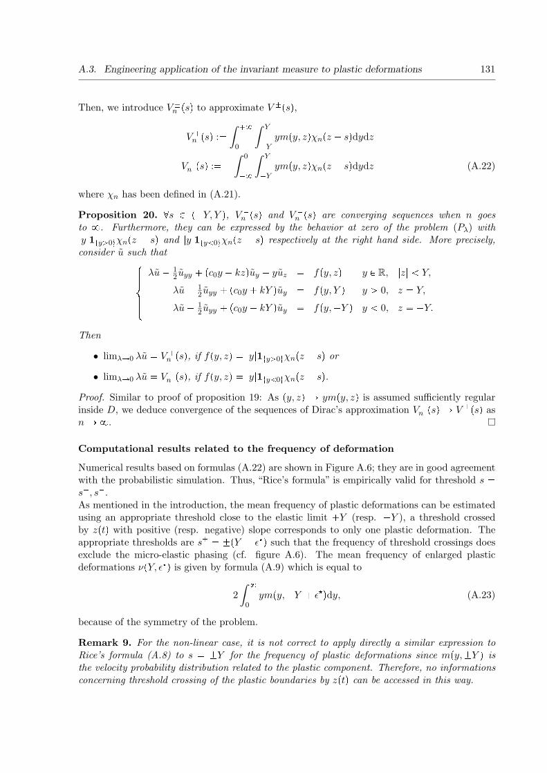
A.3. Engineering application of the invariant measure to plastic deformations 131
Then, we introduce V ✟n ♣sq to approximate V ✟♣sq,
V �n ♣sq :✏ˆ �✽
0
ˆ Y
✁Yym♣y, zqχn♣z ✁ sqdydz
V ✁n ♣sq :✏ ✁ˆ 0
✁✽
ˆ Y
✁Yym♣y, zqχn♣z ✁ sqdydz (A.22)
where χn has been defined in (A.21).
Proposition 20. ❅s P ♣✁Y, Y q, V �n ♣sq and V ✁n ♣sq are converging sequences when n goesto ✽. Furthermore, they can be expressed by the behavior at zero of the problem (Pλ) with⑤y⑤1ty→0✉χn♣z ✁ sq and ⑤y⑤1ty➔0✉χn♣z ✁ sq respectively at the right hand side. More precisely,consider u such that✩✬✬✬✫
✬✬✬✪λu✁ 1
2uyy � ♣c0y � kzquy ✁ yuz ✏ f♣y, zq y P R, ⑤z⑤ ➔ Y,
λu✁ 12uyy � ♣c0y � kY quy ✏ f♣y, Y q y → 0, z ✏ Y,
λu✁ 12uyy � ♣c0y ✁ kY quy ✏ f♣y,✁Y q y ➔ 0, z ✏ ✁Y.
Then
• limλÑ0 λu ✏ V �n ♣sq, if f♣y, zq ✏ ⑤y⑤1ty→0✉χn♣z ✁ sq or
• limλÑ0 λu ✏ V ✁n ♣sq, if f♣y, zq ✏ ⑤y⑤1ty➔0✉χn♣z ✁ sq.Proof. Similar to proof of proposition 19: As ♣y, zq Ñ ym♣y, zq is assumed sufficiently regularinside D, we deduce convergence of the sequences of Dirac’s approximation V ✟n ♣sq Ñ V ✟♣sq asnÑ✽.
Computational results related to the frequency of deformation
Numerical results based on formulas (A.22) are shown in Figure A.6; they are in good agreementwith the probabilistic simulation. Thus, “Rice’s formula” is empirically valid for threshold s ✏s✁, s�.As mentioned in the introduction, the mean frequency of plastic deformations can be estimatedusing an appropriate threshold close to the elastic limit �Y (resp. ✁Y ), a threshold crossedby z♣tq with positive (resp. negative) slope corresponds to only one plastic deformation. Theappropriate thresholds are s✟ ✏ ✟♣Y ✁ ǫ✍q such that the frequency of threshold crossings doesexclude the micro-elastic phasing (cf. figure A.6). The mean frequency of enlarged plasticdeformations ν♣Y, ǫ✍q is given by formula (A.9) which is equal to
2
ˆ ✽
0
ym♣y,✁Y � ǫ✍qdy, (A.23)
because of the symmetry of the problem.
Remark 9. For the non-linear case, it is not correct to apply directly a similar expression toRice’s formula (A.8) to s ✏ ✟Y for the frequency of plastic deformations since m♣y,✟Y q isthe velocity probability distribution related to the plastic component. Therefore, no informationsconcerning threshold crossing of the plastic boundaries by z♣tq can be accessed in this way.

132 Appendix A. An empirical study on plastic deformations
0.4 0.6 0.8 1 1.2 1.4 1.6 1.8 2 2.2 2.40
0.02
0.04
0.06
0.08
0.1
0.12
0.14
0.16
0.18
c0 = 1, k = 1
ν(Y
, ε* )
Y
PSPDE
Figure A.6: The frequency of plastic deformations ν♣Y, ǫ✍q versus Y the elasto-plastic bound.Comparison between the result given by the probabilistic simulation (PS) and the result givenby solving PDEs.
A.3.2 Empirical approach to statistics of plastic deformation
Relying on formula (A.5) and ǫ✍, we consider the following estimator of mean statistic of plasticdeformation, for any function f♣y, zq satisfying (A.14)
∆f ♣Y, ǫ✍q ✏´ 0
✁✽ f♣y,✁Y qm♣y,✁Y qdy �´✽0f♣y, Y qm♣y, Y qdy
´✽0ym♣y,✁Y � ǫ✍qdy .
Finally, we consider the following quantities
∆1♣Y, ǫ✍q ✏´✽0m♣y, Y qdy
´✽0ym♣y,✁Y � ǫ✍qdy and ∆⑤y⑤♣Y, ǫ✍q ✏
´✽0ym♣y, Y qdy
´✽0ym♣y,✁Y � ǫ✍qdy
to approximate the mean duration and the mean absolute quantity of plastic deformation.
Computational results related to statistic of plastic deformations
Shown in Figures A.7 and A.8 the curves which could be useful for engineering purpose.
A.4 Conclusion
The invariant measure has been used in this paper to study the statistical properties of theplastic deformation of an elastic perfectly plastic oscillator under standard white noise excita-tion, by means of approximation of the second marginal and “Rice’s formula”. From our studyon micro-elastic phasing, we have deduced a useful criterion for engineers to discard this phe-nomenon and to compute statistics of plastic deformation. This work has a theoretical interest

A.4. Conclusion 133
0.4 0.6 0.8 1 1.2 1.4 1.6 1.8 2 2.2 2.40.4
0.6
0.8
1
1.2
1.4
1.6
c0 = 1, k = 1, n = 8e3
∆ 1(Y, ε
* )
Y
Figure A.7: ∆1♣Y, ǫ✍q versus Y the elasto-plastic bound.
0.4 0.6 0.8 1 1.2 1.4 1.6 1.8 2 2.2 2.4
0.4
0.5
0.6
0.7
0.8
0.9
1
1.1
c0 = 1, k = 1, n = 8e3
∆ |y|(Y
, ε* )
Y
Figure A.8: ∆⑤y⑤♣Y, ǫ✍q vs Y the elasto-plastic bound.
and contributes to a further insight into the physics of the problem.
In a future work, we aim to introduce jumps (at the phase transition from plastic state toelastic state) in the dynamics of ♣y♣tq, z♣tqq, in order to overcome difficulties related to micro-elastic phasing. For such a model, ǫ✍ appears to be a good candidate for the size of the jump.

134 Appendix A. An empirical study on plastic deformations
A.5 Appendix
A.5.1 Appendix: Probabilistic algorithm of resolution of the SVI
We recall from [3] a discrete approximation of the solution to the SVI. We consider explicitknown formula related to elastic and plastic states. They are applied on random time intervalswhich are determined following the trajectory. In elastic state, the process ♣y♣tq, z♣tqq satisfies:✧
dy♣tq ✏ ✁♣c0y♣tq � kz♣tqqdt� dw♣tq,dz♣tq ✏ y♣tqdt, (A.24)
whereas in plastic state we have z♣tq ✏ ✟Y and y♣tq satisfies✧dy♣tq ✏ ✁♣c0y♣tq � kz♣tqqdt� dw♣tq,dz♣tq ✏ 0.
(A.25)
Then, there is an explicit formula to the elastic state. Let ♣y♣0q, z♣0qq ✏ ♣y, zq and ω :✏❄
4k✁c202
.Note that the condition 4k → c20 is needed so that ♣y♣tq, z♣tqq have real valued solutions. Wehave ✩✬✬✬✫
✬✬✬✪y♣tq ✏ ✁ c0
2z♣tq � e✁
c0t
2 t✁ωz sin ♣ωtq � ♣y � c02zq cos ♣ωtq✉
� ´ t0e✁
c02♣t✁sq cos ♣ω♣t✁ sqqdw♣sq,
z♣tq ✏ e✁c0t
2 tz cos ♣ωtq � 1ω♣y � c0
2zq sin ♣ωtq✉
� 1ω
´ t
0e✁
c02♣t✁sq sin ♣ω♣t✁ sqqdw♣sq.
(A.26)
y♣tq is a gaussian variable of mean ey♣t, z, yq and variance σ2y♣tq, where
ey♣t, y, zq ✏ ✁c02ez♣t, y, zq � e✁
c0t
2 t✁ωz sin ♣ωtq � ♣y � c0
2zq cos ♣ωtq✉,
σ2y♣tq ✏
ˆ t
0
e✁c0s cos2 ♣ωsqds✁ c204ω2
ˆ t
0
e✁c0s sin2 ♣ωsqds✁ c0
2ω2e✁c0t sin2 ♣ωtq.
z♣tq is a gaussian variable of mean ez♣t, z, yq and variance σ2z♣tq, where
ez♣t, y, zq ✏ e✁c0t
2 tz cos ♣ωtq � 1
ω♣y � c0
2zq sin ♣ωtq✉,
σ2z♣tq ✏ 1
ω2
ˆ t
0
e✁c0s sin2 ♣ωsqds.
The correlation between y♣tq and z♣tq are given by
σyz♣tq ✏ 1
2ω
ˆ t
0
e✁c0s sin ♣2ωsqds✁ c0
2ω2
ˆ t
0
e✁c0s sin2 ♣ωsqds.
In plastic state, we also have an explicit formula. Let ♣y♣0q, z♣0qq ✏ ♣y,✟Y q then★y♣tq ✏ ye✁c0t ✠ kY
c0♣1✁ e✁c0tq � e✁c0t❄
2c0w♣e2c0t ✁ 1q,
z♣tq ✏ ✟Y. (A.27)
Considering explicit solutions, a C code has been written to simulate ♣y♣tq, z♣tqq. Let T → 0, N PN, and ♣tnqn✏0..N be a family of time which disretize r0, T s, such that tn ✏ nδt where δt :✏ T
N.

A.5. Appendix 135
We set Σ P M2,2♣R2q such that
ΣΣT ✏✂σ2y♣δtq σyz♣δtq
σyz♣δtq σ2z♣δtq
✡. (A.28)
Let ♣Gn,mqn✏0..N,m✏1,2 a family of independent gaussian variables N ♣0, 1q. Gaussian variablesare generated using Box-Muller formula [23] and the C function random(). Initialize ♣yδt0 , zδt0 q ✏♣y, zq, the finite difference scheme for (A.10) is written in the following manner:
For n ✏ 0, 1, .. with θδt0 ✏ τ δt0 ✏ 0, we define two sequences of δt-stopping time:★θδtn�1 :✏ infttk → τ δtn ⑤ ⑤zδttk ⑤ ✏ Y ✉τ δtn�1 :✏ infttk → θδtn�1 ⑤ ⑤zδttk ⑤ ➔ Y ✉
(A.29)
• When tk P rτ δtn , θδtn�1r, we have ⑤zδttk ⑤ ➔ Y , we set
✂yk�1
zk�1
✡:✏
✂ey♣δt, y♣tkq, z♣tkqqez♣δt, y♣tkq, z♣tkqq
✡� Σ
✂Gk,1Gk,2
✡(A.30)
– If ⑤zk�1⑤ ➔ Y then ✂yδttk�1
zδttk�1
✡:✏
✂yk�1
zk�1
✡(A.31)
– If ⑤zk�1⑤ ➙ Y then ✂yδttk�1
zδttk�1
✡:✏
✂yk�1
σk�1Y
✡(A.32)
where σk�1 :✏ sign♣zk�1q.• When tk P rθδtn�1, τ
δtn�1r, we have σkz
δttk✏ Y ,
– If σkyδttk→ 0, then we set
✂yk�1
zk�1
✡:✏
✄yδttke
✁c0δt ✠ kYc0♣1✁ e✁c0δtq � e✁c0δt
❜e2c0δt✁1
2c0Gk,1
σkY
☛(A.33)
∗ If σkyk�1 → 0, then ✂yδttk�1
zδttk�1
✡:✏
✂yk�1
σkY
✡(A.34)
∗ If σkyk�1 ➔ 0, then ✂yδttk�1
zδttk�1
✡:✏
✂0
σkY
✡(A.35)
– Else, we set ✂yk�1
zk�1
✡:✏
✂ey♣δt, 0, σkY qez♣δt, 0, σkY q
✡� Σ
✂Gk,1Gk,2
✡(A.36)
∗ If ⑤zk�1⑤ ➔ Y , then ✂yδttk�1
zδttk�1
✡:✏
✂yk�1
zk�1
✡(A.37)

136 Appendix A. An empirical study on plastic deformations
∗ If ⑤zk�1⑤ ➙ Y , then ✂yδttk�1
zδttk�1
✡:✏
✂yk�1
σkY
✡(A.38)
Remark 10. Simulations do not deal with a true white noise. Indeed, because of the step ofdiscretization, the noise is filtered. The ideal case would be to take δt as small as possible, butour probabilistic algorithm is too slow to get satisfactory results in this way. Thus we cannotconsider δt below than 10✁6.
Acknowledgments
We would like to thank Alain Bensoussan, Laurent Borsoi, Stephane Menozzi and Olivier Piron-neau for their useful advices.

List of Figures
1 Vibration d’un troncon de tuyauterie : Illustration de la vibration d’untroncon de ligne de tuyauterie sur une table d’experimentation du CEA (Labora-toire d’Etudes de Mecanique SIsmique,EMSI). La structure est installee sur unplateau qui simule l’action sismique. La reponse de la structure a cette sollic-itation presente une alternance entre les phases de deformation elastique et lesphases de deformation plastique. Ici, la deformation permanente se manifeste auxcoudees basses de la tuyauterie. . . . . . . . . . . . . . . . . . . . . . . . . . . . . 3
2 Excitation sismique / deplacement elasto-plastique : Comparaison en-tre le test experimental et la reponse du modele a une dimension : enhaut, un signal d’excitation sismique et en bas la superposition des deux reponsesa ce signal fournies par un test experimental (deplacement de la masse situee entete de la tuyauterie, Figure 1) et par la reponse d’un oscillateur non-lineaire. . . 4
1.1 From the top to the bottom: λuλ for λ ✏ 1.0 and λ ✏ 10✁1, with g♣y, zq ✏1
2πσzσye✁ 1
2z2
σ2z e
✁ 12
y2
σ2y and σz ✏ σy ✏
❛1④200. . . . . . . . . . . . . . . . . . . . . . 29
1.2 From the top to the bottom: λuλ for λ ✏ 10✁4 and λ ✏ 10✁9, with g♣y, zq ✏1
2πσzσye✁ 1
2z2
σ2z e
✁ 12
y2
σ2y and σz ✏ σy ✏
❛1④200. . . . . . . . . . . . . . . . . . . . . . 30
1.3 From the top to the bottom: λuλ for λ ✏ 1.0 and λ ✏ 10✁1, with g♣y, zq ✏1
2πσzσye✁ 1
2
♣z✁Y q2σ2
z e✁ 1
2
y2
σ2y and σz ✏ σy ✏
❛1④200. . . . . . . . . . . . . . . . . . . . 31
1.4 From the top to the bottom: λuλ for λ ✏ 10✁4 and λ ✏ 10✁9, with g♣y, zq ✏1
2πσzσye✁ 1
2
♣z✁Y q2σ2
z e✁ 1
2
y2
σ2y and σz ✏ σy ✏
❛1④200. . . . . . . . . . . . . . . . . . . . 32
1.5 mN computed by the Ultra Weak Method, from the top to the bottom we considerY ✏ 1, 2. When Y increases the plastic part decreases. . . . . . . . . . . . . . . . 33
1.6 mN computed by the Ultra Weak Method, from the top to the bottom we considerY ✏ 3, 4. When Y increases the plastic part decreases. . . . . . . . . . . . . . . . 34
1.7 Example of trajectory ♣y♣tq, z♣tqqtPr0,T s, T ✏ 10. . . . . . . . . . . . . . . . . . . . 37
1.8 Plots of mMC computed by the Monte-Carlo Method; from the top to the bottomwe consider Y ✏ 1, 2. When Y increases the plastic part decreases, indeed pMC
1 ✏84.9r84.7,85.0s%, pMC
2 ✏ 9.62r9.61,9.63s% . . . . . . . . . . . . . . . . . . . . . . . . . 38
1.9 Plots of mMC computed by the Monte-Carlo Method; from the top to the bottomwe consider Y ✏ 3, 4. When Y increases the plastic part decreases, indeed pMC
3 ✏0.04764r0.04760,0.04768s%, pMC
4 ✏ 0.0 %. . . . . . . . . . . . . . . . . . . . . . . . . 39
137

138 List of Figures
1.10 Top: L2-Relative error :⑥mMC✁mN ⑥
L2
⑥mMC⑥L2between the result given by the Monte-
Carlo method and the results given by the Ultra Weak method, versus❄N , where
N is the number of basis functions. Bottom: The same plot in log-log scale. . . . 401.11 Visualization of Micro-Elastic Phasing Phenomenon: At the top-left we have sam-
ple trajectory of ♣t, z♣tqq, at the top-right we have the corresponding trajectory♣y♣tq, z♣tqq in the phase space; we observe regular elastic and plastic phasing. Atthe bottom in the both cases, a zoom on plastic phasing reveals an illustrativemicro-elastic phasing. . . . . . . . . . . . . . . . . . . . . . . . . . . . . . . . . . 42
1.12 Un♣sq,Wn♣sq, s P ♣✁Y, Y q and location of s✟, Y ✏ 1. . . . . . . . . . . . . . . . . 431.13 Un♣sq,Wn♣sq, s P ♣✁Y, Y q and location of s✟, Y ✏ 1.5. . . . . . . . . . . . . . . . 431.14 Un♣sq,Wn♣sq, s P ♣✁Y, Y q and location of s✟, Y ✏ 2. . . . . . . . . . . . . . . . . 44
A.1 Visualization of Micro-Elastic Phasing Phenomenon: At the top-left we have sam-ple trajectory of ♣t, z♣tqq, at the top-right we have the corresponding trajectory♣y♣tq, z♣tqq in the phase space; we observe regular elastic and plastic phasing. Atthe bottom in the both cases, a zoom on plastic phasing reveals an illustrativemicro-elastic phasing. . . . . . . . . . . . . . . . . . . . . . . . . . . . . . . . . . 124
A.2 Un♣sq,Wn♣sq, s P ♣✁Y, Y q and location of s✟, Y ✏ 1. . . . . . . . . . . . . . . . . 129A.3 Un♣sq,Wn♣sq, s P ♣✁Y, Y q and location of s✟, Y ✏ 1.5. . . . . . . . . . . . . . . . 129A.4 Un♣sq,Wn♣sq, s P ♣✁Y, Y q and location of s✟, Y ✏ 2. . . . . . . . . . . . . . . . . 130A.5 Y vs s� at left; Y vs ǫ✍④Y at right. . . . . . . . . . . . . . . . . . . . . . . . . . . 130A.6 The frequency of plastic deformations ν♣Y, ǫ✍q versus Y the elasto-plastic bound.
Comparison between the result given by the probabilistic simulation (PS) and theresult given by solving PDEs. . . . . . . . . . . . . . . . . . . . . . . . . . . . . . 132
A.7 ∆1♣Y, ǫ✍q versus Y the elasto-plastic bound. . . . . . . . . . . . . . . . . . . . . . 133A.8 ∆⑤y⑤♣Y, ǫ✍q vs Y the elasto-plastic bound. . . . . . . . . . . . . . . . . . . . . . . . 133

List of Tables
3.1 Monte-Carlo simulations to compare numerical solution of the left and right handsides of (3.4), T ✏ 500 , δt ✏ 10✁4 and MC ✏ 5000. . . . . . . . . . . . . . . . . 59
A.1 Frequency of occurence, mean duration and mean absolute value of the deforma-tion and time required to obtain M ✏ 10000 enlarged plastic phases versus ǫ.Thedependency on ǫ is clear. . . . . . . . . . . . . . . . . . . . . . . . . . . . . . . . . 126
139

140 List of Tables

Bibliography
[1] A. Bensoussan, H. Jasso-Fuentes, S. Menozzi, L. Mertz Asymptotic analysis of stochasticvariational inequalities modeling an elasto-plastic problem with vanishing jumps, submitted.
[2] A. Bensoussan, J-L. Lions. Controle impulsionnel et inequations quasi variationnelles.Dunod, Paris 1982.
[3] A. Bensoussan, L. Mertz, O. Pironneau, J. Turi, An Ultra Weak Finite Element Method asan Alternative to a Monte Carlo Method for an Elasto-Plastic Problem with Noise, SIAMJ. Numer. Anal. , 47(5) (2009), 3374–3396.
[4] A. Bensoussan, L. Mertz, Degenerate Dirichlet problems related to the ergodic theory foran elasto-plastic oscillator excited by a filtered white noise, submitted.
[5] A. Bensoussan, L. Mertz, An analytic approach to the ergodic theory of stochastic variationalinequalities, submitted.
[6] A. Bensoussan, L. Mertz Behavior of the plastic deformation of an elasto-perfectly-plasticoscillator with noise, submitted.
[7] A. Bensoussan, J. Turi, Degenerate Dirichlet Problems Related to the Invariant Measure ofElasto-Plastic Oscillators, Applied Mathematics and Optimization, 58(1) (2008), 1–27.
[8] A. Bensoussan, J. Turi, On a Class of Partial Differential Equations with Nonlocal DirichletBoundary Conditions, Appl. Num. Par. Diff. Eq. 15, pp. 9-23.
[9] C. Bernardi, V. Girault, F. Hecht, H. Kawarada, O. Pironneau, A finite element problemissued from fictitious domain techniques, East-West J. Numer. Math. 9 (4) (2001) 253-263.
[10] B.K. Bathia, E.H. Vanmarcke, Associate linear system approach to nonlinear randomvibration, J. Engrg. Mech., ASCE, 117, (1991), 2407-2428.
[11] L. Borsoi, P. Labbe Approche probabiliste de la ruine d’un oscillateur elasto-plastique sousseisme. 2eme colloque national de l’AFPS. 18-20 Avril 1989.
[12] G.Q. Cai, Y.K. Lin, On randomly excited hysteretic structures, J. of Applied Mechanics,ASME 57, (1990), 442-448.
[13] T.K. Caughey, Nonlinear theory of random vibrations, Adv. in Appl. Mech.11, C.S. Yih(ed.), Academic Press, (1971), 209-253.
[14] O. Ditlevsen, Elasto-Plastic oscillator with Gaussian excitation, J. of Engrg. Mech., ASCE,112, (1986), 386-406.
141

142 Bibliography
[15] O. Ditlevsen, L. Bognar, Plastic displacement distributions of the Gaussian white noiseexcited elasto-plastic oscillator, Prob. Eng. Mech. 8, (1993), 209-231.
[16] O.Ditlevsen, N. Tarp-Johansen, White noise excited non-ideal elasto-plastic oscillator, ActaMechanica 125, (1997), 31-48.
[17] J.L. Doob, Stochastic Processes, Wiley, New York,1953.
[18] G. Duvaut, J.L. Lions, Inequalities in Mechanics and Physics, Springer-Verlag, New-York,1976.
[19] C.Feau, Les methodes probabilistes en mecanique sismique. Applications aux calculs detuyauteries fissurees, These CEA-Universite d’Evry.
[20] C. Feau, Probabilistic response of an elastic perfectly plastic oscillator under Gaussianwhite noise, Probabilistic Engineering Mechanics, 23(1) (2008),36–44.
[21] C. Feau, L. Mertz An empirical study on plastic deformations of an elasto-plastic problemwith noise, submitted.
[22] FREEFEM++, http://www.freefem.org/
[23] P. Glasserman, Monte Carlo Methods in Financial Engineering, Series: Stochastic Mod-elling and Applied Probability , Vol. 53 2003, XIV, 602 p. 70 illus., Hardcover ISBN:978-0-387-00451-8.
[24] R. Grossmayer, Stochastic analysis of elasto-plastic systems, J. Engrg. Mech., ASCE, 39,(1981), 97-115.
[25] I. Karatzas, S.E. Shreve, Brownian Motion and Stochastic Calculus, 2nd edition, Springer1991.
[26] D. Karnopp, T.D. Scharton, Plastic deformation in random vibration, The Journal of theAcoustical Society of America, 39 (1966), 1154-61.
[27] Khasminkii, R.Z., Stochastic Stability of Differential Equations, Sitjhoff and Noordhoff,The Netherlands (1980).
[28] B. Lazarov, O. Ditlevsen, Slepian simulation of distributions of plastic displacements ofearthquake excited shear frames with large number of stories, Prob. Eng. Mech. 20, (2005),251-262.
[29] R.H. Lyon On the vibration statistics of a randomly excited hard-spring oscillator II, J.Acoust. Soc. Amer. 33 (1961), 1395-1403.
[30] A. Preumont, Random Vibration and Spectral Analysis, Kluwer, Boston, 1994.
[31] S.O. Rice, Mathematical Analysis of Random Noise, 1944.
[32] J.B. Roberts, The response of an oscillator with bilinear hysteresis to stationary randomexcitation, J. of Applied Mechanics 45, (1978), 923-928.
[33] J.B. Roberts, Reliability of randomly excited hysteretic systems, Mathematical Modelsfor Structural Reliability Analysis, F. Casciati and J.B. Roberts (eds.), CRC Press, 1996,139-194.

143
[34] J.B. Roberts, P.D. Spanos, Random Vibration and Statistical Linearization, Wiley andSons, Chichester, U.K., 1990.
[35] B.F. Spencer, Reliability of Randomly Excited Hysteretic Structures, Springer-Verlag,Berlin, 1986.
[36] E.H. Vanmarcke, On the distribution of the first-passage time for stationary random pro-cesses, Journal of Applied Mechanics, (1975), 215–220.
[37] E.H. Vanmarcke, Random Fields; Analysis and Synthesis, The MIT Press, 2nd edition,1984.

144 Bibliography

Resume
Cette these traite des inequations variationnelles stochastiques et de leurs applications aux vi-brations de structures mecaniques. On considere d’abord un algorithme numerique deterministepour obtenir le regime stationnaire d’une inequation variationnelle stochastique modelisant unoscillateur elasto-plastique excite par un bruit blanc. Une famille de solutions d’equations auxderivees partielles definissant la mesure invariante par dualite est etudiee comme alternative a lasimulation probabiliste. Puis, nous presentons une nouvelle caracterisation de l’unique mesureinvariante. Dans ce contexte, nous montrons une relation liant des problemes non-locaux et desproblemes locaux en introduisant la definition des cycles courts. Dans un cadre oriente vers lesapplications, nous demontrons que la variance de la deformation plastique croıt lineairementavec le temps et nous caracterisons rigoureusement le coefficient de derive en introduisant ladefinition des cycles longs. Dans la suite, nous etudions un processus approche de la solutionde l’inequation comportant des sauts aux instants de transition de l’etat plastique vers l’etatelastique. Nous prouvons que la solution approchee converge sur tout intervalle de temps finivers la solution de l’inequation, lorsque la taille du saut tend vers 0. Ensuite, nous definissonsune inequation variationnelle stochastique pour modeliser un oscillateur elasto-plastique excitepar un bruit blanc filtre. Nous prouvons la propriete ergodique du processus sous-jacent etnous caracterisons sa mesure invariante. Nous etendons la methode de A.Bensoussan et J.Turiavec une difficulte supplementaire due a l’accroissement de la dimension. Finalement, dans unchapitre oriente vers l’experimentation numerique, nous mettons en evidence par les simulationsprobabilistes le phenomene de phases micro-elastiques. Leur impact concerne des grandeursutiles a l’ingenieur comme la frequence des deformations plastiques. Un critere empirique quipeut etre utile a l’ingenieur est fourni afin ne pas prendre en compte les phases micro-elastiqueset ainsi evaluer d’une facon realiste, a partir de la mesure invariante, les statistiques de la de-formation plastique d’un oscillateur elasto-plastique excite par un bruit blanc.
Mots-cles : inequations variationnelles stochastiques, equations aux derivees partielles avecdes conditions non-locales, vibrations aleatoires, diffusion ergodique.

Abstract
This work is devoted to stochastic variational inequalities and their applications to random vi-brations of mechanical structures. First, an efficient method for obtaining numerical solutions ofa stochastic variational inequality modeling an elasto-plastic oscillator with noise is considered.Since Monte Carlo simulations for the underlying stochastic process are too slow, as an alterna-tive, approximate solutions of the partial differential equation defining the invariant measure ofthe process are studied. Next, we present a new characterization of the invariant measure. Thekey finding is the connection between nonlocal partial differential equations and local partialdifferential equations which can be interpreted with short cycles of the Markov process solutionof the stochastic variational inequality. For engineering applications, we prove that plastic defor-mation for an elasto-perfectly-plastic oscillator has a variance which increases linearly with timeand we characterize the corresponding drift coefficient by defining long cycles behavior of theMarkov process solution of the stochastic variational inequality. A major advantage of stochasticvariational inequality is to overcome the need to describe the trajectory by phases (elastic orplastic). This is useful, since the sequence of phases cannot be characterized easily. However,it remains important to have informations on these phases. In order to reconcile these contra-dictory issues, we introduce an approximation of stochastic variational inequalities by imposingartificial small jumps between phases allowing a clear separation of the phases. We prove thatthe approximate solution converges on any finite time interval, when the size of jump tends to0. Then to study a more general case, a stochastic variational inequality is proposed to modelan elasto-plastic oscillator excited by a filtered white noise. We prove the ergodic property ofthe process and characterize the corresponding invariant measure. This extends Bensoussan-Turi’s method with a significant additional difficulty of increasing the dimension. Finally, ina last chapter oriented to numerical experiments, we exhibit by probabilistic simulations thephenomenon of micro-elastic phases. The main difficulty related to micro-elastic phasing is thatthey interfere on quantities of interest such that frequency of plastic deformations. An interest-ing criterion is provided which could be useful in engineering problems to discard micro-elasticphases and to evaluate statistics of plastic deformations of an elasto-plastic oscillator white noiseexcited.
Keywords: stochastic variational inequalities, partial differential equations with nonlocalconditions, random vibration, ergodic diffusions.