US YIELD FORECASTING USING CROP CONDITION RATINGS

BY

FERNANDA de BARROS DIAS

THESIS

Submitted in partial fulfillment of the requirements

for the degree of Master of Science in Agricultural and Applied Economics

in the Graduate College of the

University of Illinois at Urbana-Champaign, 2017

Urbana, Illinois

Master’s Committee:

Professor Scott Irwin, Chair

Professor Gary Schnitkey

Professor Emeritus Darrel Good

ii

ABSTRACT

This thesis studied the relationship between US average yield for the five main crops

grown in the United States, corn, soybeans, upland cotton, winter wheat, and spring wheat, and

crop condition ratings from 1986 to 2015. Three statistical models were tested, the first one

including all categories of condition ratings, a trend, and no intercept. The second model

addresses the issue of abandoned acres following the ideas of Fackler & Norwood and included

all categories less the Very Poor category, a trend, and no intercept. The last model investigated

is the sum of Good and Excellent categories, a trend, and intercept. The models were used to

forecast US yield out-of-sample as an alternative to the benchmark forecast WASDE. Major

findings include: 1) crop condition ratings will not be a good predictor of US average yield if

there is an increase in the WASDE yield forecasting and the conditions are not aligned

accordingly, 2) when weather becomes an issue these models perform very well compared to

WASDE as it was the case in 2012, 3) the models are a good forecast beating the USDA

WASDE in almost every instance for the trend-yield months, 4) almost in every instance the best

performing model did not use USDA’s original ratings, which implies that the corrections made

to the data are rational, 5) except for soybeans and spring wheat, the WASDE survey-yield

months are a better forecast than the statistical models developed in this thesis given the nature

of the commodities and USDA’s superior method, 6) weighting by production instead of planted

acres becomes particularly important when there is a wide range of yield variability between

states like it is the case for corn and winter wheat, 7) correction for bias becomes particularly

important the more the crop is sensitive to adverse events that affect yield during its reproduction

stage.

iii

TABLES OF CONTENTS

LIST OF TABLES…………………………………………………………………………...vii

LIST OF FIGURES…………………………………………………………………………...x

1. INTRODUCTION………………………………………………………………………...1

1.1 Background…………………………………………………………………………....1

1.2 Objectives ………………………………………………………………………….…3

1.3 Data and Method…………………………………………………………………..…..4

1.4 Overview………………………………………………………………………..……..5

2. REVIEW OF THE LITERATURE……………………………………………………….6

2.1 Introduction…………………………………………………………………………....6

2.2 Agronomy Theory………………………………………………………………….….6

2.3 Remote Sensing ……………………………………………………………………..10

2.4 Crop Weather……………………………………………………………………..….13

2.5 Crop Condition Models…………………………………………………………...…16

2.6 Summary……………………………………………………………………………..24

3. DATA……………………………………………………………………………………28

3.1 Introduction…………………………………………………………………………..28

3.2 The Crop Progress and Condition Report…………………………………………....28

3.3 The Crop Progress and Condition Report Production…………………………….…29

3.4 Yield, Production, Crop Condition Ratings, and Locations Analyzed………………31

iv

3.5 Descriptive Analysis of the Data…….……………......……………………….……32

3.5.1 Corn……………………………………………………………………....34

3.5.2 Soybeans………………………………………………………………....36

3.5.3 Upland Cotton………………………………………………………..…..38

3.5.4 Winter Wheat………………………...…………………………………..39

3.5.5 Spring Wheat………………………………………….………………....40

3.5.6 Yields…………………………………………………………...…….….41

3.6 Summary……………..……………………………………………………………....42

4. MODELS AND IN-SAMPLE ANALYSIS …….……………………………..…….….43

4.1 Introduction…………………………………………………………………………..43

4.2 Conceptual Framework……………………………………………………………....43

4.3 Results for Corn…………………………………………………………………..….47

4.4 Results for Soybeans…………………………………………………………………48

4.5 Results for Upland Cotton………………………………………………………..….49

4.6 Results for Winter Wheat……………………………………………………….....…50

4.7 Results for Spring Wheat…………………………………………………………….51

4.8 Summary………………………………………………………………………..……52

5. A YIELD FORECASTING COMPETITION………………………….…..…………...55

5.1 Introduction………………………………………………………………………..…55

5.2 Development of the Yield Prediction Competition………………………………….55

5.2.1 Original Crop Condition Ratings…………………………………….…….55

5.2.2 Bias Adjustment……………………………………………………………56

v

5.2.3 Production Weights…………………………………………………..…….56

5.3 Evaluation Standards………………………………………………………….……..57

5.4 Forecasting Results…………………………………………………………………..58

5.4.1 Corn Yield Forecasts Results Model Comparison………………………....59

5.4.2 Corn Yield Forecasts Results Best Performing Model vs. WASDE………61

5.4.3 Soybean Yield Forecasts Results Model Comparison…………..................62

5.4.4 Soybean Yield Forecasts Results Best Performing Model vs. WASDE…..63

5.4.5 Upland Cotton Yield Forecasts Results Model Comparison………………63

5.4.6 Upland Cotton Yield Forecasts Results Best Performing Model vs.

WASDE………………………………………………………………………….64

5.4.7 Winter Wheat Yield Forecasts Results Model Comparison……………….65

5.4.8 Winter Wheat Yield Forecasts Results Best Performing Model vs.

WASDE………………………………………………………………………….66

5.4.9 Spring Wheat Yield Forecasts Results Model Comparison…….………….66

5.4.10 Spring Wheat Yield Forecasts Results Best Performing Model vs.

WASDE………………………………………………………………………….67

5.5 Summary…………………………………………………………………….……….68

6. CONCLUSION…………………………….……………………………………………..69

6.1 Review…………………………………………………………………………..…...69

vi

6.2 Summary of Findings……………………………………………………………...…70

6.3 Future Work and Concluding Remarks…………………………………………..….72

FIGURES AND TABLES…………………………………………………………………...75

REFERENCES……………………………………………………………………………..165

vii

LIST OF TABLES

Table 1. Corn- Mean and St. Deviation Difference between the last week and other week’s

ratings during the year per category……………………………………………………………...80

Table 2. Soybeans- Mean and St. Deviation Difference between the last week and other week’s

ratings during the year per category……………………………………………………………...83

Table 3. Cotton, Upland- Mean and St. Deviation Difference between the last week and other

week’s ratings during the year per category……………………………………………………..86

Table 4. Winter Wheat- Mean and St. Deviation Difference between the last week and other

week’s ratings during the year per category…………………………………………………..…89

Table 5. Spring Wheat- Mean and St. Deviation Difference between the last week and other

week’s ratings during the year per category…………………………………………………..…92

Table 6. National Level Coefficients Estimates for Corn, 1986-2015………………………....130

Table 7. National Level Coefficients Estimates for Soybeans, 1986-2015………………….....131

Table 8. National Level Coefficients Estimates for Cotton Upland, 1986-2015……………….132

Table 9. National Level Coefficients Estimates for Winter Wheat, 1986-2015……………..…133

Table 10. National Level Coefficients Estimates for Spring Wheat, 1986-2015…………...….134

Table 11. Corn Yield Forecast Weekly Errors 2006-2015……………………………………..135

Table 12. Corn Yield Forecast Weekly Errors 2006-2015 MAPE RATIO………………….…136

viii

Table 13. Corn Yield Forecast Weekly Errors 2006-2015……………………………………..137

Table 14. Corn Yield Forecast Weekly Errors 2006-2015 RMSPE RATIO…………………...138

Table 15. Soybean Yield Forecast Weekly Errors 2006-2015…………………………………139

Table 16. Soybean Yield Forecast Weekly Errors 2006-2015 MAPE RATIO……………...…140

Table 17. Soybean Yield Forecast Weekly Errors 2006-2015………………………………....141

Table 18. Soybean Yield Forecast Weekly Errors 2006-2015 RMSPE RATIO…………….....142

Table 19. Cotton, Upland Yield Forecast Weekly Errors 2006-2015…………………………..143

Table 20. Cotton, Upland Yield Forecast Weekly Errors 2006-2015 MAPE RATIO………....144

Table 21. Cotton, Upland Yield Forecast Weekly Errors 2006-2015…………………………..145

Table 22. Cotton, Upland Yield Forecast Weekly Errors 2006-2015 RMSPE RATIO………..146

Table 23. Winter Wheat Yield Forecast Weekly Errors 2006-2015………………………..…..147

Table 24. Winter Wheat Yield Forecast Weekly Errors 2006-2015 MAPE RATIO……….….148

Table 25. Winter Wheat Yield Forecast Weekly Errors 2006-2015…………………………....149

Table 26. Winter Wheat Yield Forecast Weekly Errors 2006-2015 RMSPE RATIO…………150

Table 27. Spring Wheat Yield Forecast Weekly Errors 2006-2015…………………………....151

Table 28. Spring Wheat Yield Forecast Weekly Errors 2006-2015 MAPE RATIO………..….152

Table 29. Spring Wheat Yield Forecast Weekly Errors 2006-2015…….……………………...153

Table 30. Spring Wheat Yield Forecast Weekly Errors 2006-2015 RMSPE RATIO……….…154

ix

Table 31. Corn Yield Forecast Error Comparison 2006-2015……………………………...…..155

Table 32. Corn Yield Forecast Error Comparison 2006-2015……………………………….....156

Table 33.Soybean Yield Forecast Error Comparison 2006-2015……………………………....157

Table 34. Soybean Yield Forecast Error Comparison 2006-2015…………………………...…158

Table 35. Cotton, Upland Yield Forecast Error Comparison 2006-2015……………………....159

Table 36. Cotton, Upland Yield Forecast Error Comparison 2006-2015………………………160

Table 37. Winter Wheat Yield Forecast Error Comparison 2006-2015………………………..161

Table 38. Winter Wheat Yield Forecast Error Comparison 2006-2015……………………..…162

Table 39. Spring Wheat Yield Forecast Error Comparison 2006-2015…………………….…..163

Table 40. Spring Wheat Yield Forecast Error Comparison 2006-2015…………………….…..164

x

LIST OF FIGURES

Figure 1. Corn- Condition Ratings Mean for Each Category for Years 1986 to 2015, Beginning,

Middle, and End of the Season…………………………………………………………………. 75

Figure 2. Soybeans- Condition Ratings Mean for Each Category for Years 1986 to 2015,

Beginning, Middle, and End of the Season………………………………………………………76

Figure 3. Cotton, Upland- Condition Ratings Mean for Each Category for Years 1986 to 2015,

Beginning, Middle, and End of the Season………………………………………………………77

Figure 4. Winter Wheat- Condition Ratings Mean for Each Category for Years 1986 to 2015,

Beginning, Middle, and End of the Season………………………………………………………78

Figure 5. Spring Wheat- Condition Ratings Mean for Each Category for Years 1986 to 2015,

Beginning, Middle, and End of the Season………………………………………………………79

Figure 6. Corn- Mean Difference of Ratings for Each Category per Week for Years 1986 to

2015, June 2-39……………………………………………………………………………...…...95

Figure 7. Soybeans- Mean Difference of Ratings for Each Category per Week for Years 1986 to

2015, June 16-39…………………………………………………………………………….…...98

Figure 8. Cotton, Upland- Mean Difference of Ratings for Each Category per Week for Years

1986 to 2015, June 16-39…………………………………………………………………….…101

Figure 9. Winter Wheat- Mean Difference of Ratings for Each Category per Week for Years

1986 to 2015, April 7-25………………………………………………………………….….…104

xi

Figure 10. Spring Wheat- Mean Difference of Ratings for Each Category per Week for Years

1986 to 2015, June 9-31……………………………………………………………………...…107

Figure 11. Corn- Standard Deviation of Ratings per Week, 1986-2015……………………….110

Figure 12. Soybeans- Standard Deviation of Ratings per Week, 1986-2015…………………..113

Figure 13. Cotton, Upland- Standard Deviation of Ratings per Week, 1986-2015…………….116

Figure 14. Winter Wheat- Standard Deviation of Ratings per Week, 1986-2015……………...119

Figure 15. Spring Wheat- Standard Deviation of Ratings per Week, 1986-2015……………...122

Figure 16. Average U.S Corn Yield, 1986-2015……………………………………………….125

Figure 17. Average U.S Soybean Yield, 1986-2015…………………………………………...126

Figure 18. Average U.S Cotton, Upland Yield, 1986-2015…………………………………….127

Figure 19. Average U.S Winter Wheat Yield, 1986-2015……………………………………...128

Figure 20. Average U.S Spring Wheat Yield, 1986-2015……………………………………...129

1

1. INTRODUCTION

1.1 Background

Crop yield forecasting is of main concern for market participants from farmers to

commercial trading companies, such as large agricultural companies, and non-commercial

trading companies, such as hedge funds. Early season production forecast is key to price

discovery mechanism for those billion dollar crops. Yield forecast has major impact on

positions taken in the market according to what is the anticipated supply of crops and the given

demand. Not many studies have truly forecasted yield out of sample and compared to a

benchmark forecast such as the one provided by the USDA World Agricultural Supply and

Demand Estimates (WASDE).

Furthermore, crop condition ratings are the most widely used indicator of yield potential by

market participants throughout the growing season of crops, however, little research has been

done using the ratings. Lehecka (2014) investigated the informational value of the crop condition

ratings during report release days and non-report release days finding significant differences in

return variabilities between the two proving the impact of the weekly release of crop condition

ratings has on market participants. Only two previous studies, Kruse & Smith and Fackler &

Norwood, have analyzed crop condition ratings as a forecasting tool but at the time of their

research there was not enough observations to make an out-of-sample forecast. The estimates in

both papers were in-sample, therefore, not aligned with the USDA WASDE, which is a true

forecast. This thesis aims to fill the gap in the literature of using crop condition ratings to make

out of sample yield forecast of the main commodities grown in the United States.

Other lines of research have mainly focused on agronomy simulation models that

incorporate complex mathematical equations and demand difficult inputs for calibration of the

2

model. Furthermore, these models are usually not made to be applicable at a large regional scale

making it problematic to obtain a forecast of yield on the national or state level. Remote sensing

imagery of crops is another method that has been applied to forecast yield but the technique

needs improvement in its spatial resolution and cost-effectiveness since the technique is not

widely available to a wide range of market participants. The hybrid of those two facets of

research showed improvement over the use of only one or another but still remain ineffective in

conveying useful information for market participants’ decision making in a timely manner.

Empirical studies, on the other hand, make use of information that incorporates the

determinants of crop yield in a broad sense. For instance, the USDA crop condition ratings data

used in this thesis conveys information about how the crops are developing responding to a

variety of events throughout the growing season such as weather, pests and diseases, and it is

reported every week from April to November, as mentioned before, being the most widely

used indicator of yield potential.

As mentioned before, this thesis focuses mainly on the ideas developed by Kruse and Smith

(1994) and Fackler and Norwood (1999). Kruse and Smith associated a given set of yields to

each of the categories Very Poor, Poor, Fair, Good and Excellent condition of crops included

in the Crop Progress and Condition Report of the USDA. The authors developed a weighted

maximum likelihood method to estimate the set of soybean and corn yields associated with

each category. Fackler and Norwood develop a method of weighting the percentage of yields in

each category. They also solved the issue that yield forecasts can increase when crop

conditions worsen by eliminating the Very Poor category considering them abandoned acres.

Yet, the comparisons made in both papers are not completely aligned with the USDA’s

3

forecasts given that the USDA provides real forecasts while these paper’s forecasts are in-

sample.

Empirical studies emphasize statistical evidence and are conveniently used given its

simplicity and timeliness compared to experimental type of data obtained in agronomy studies

or remote sensing imagery. However, empirical studies might overlook information such as

plant physiology obtained by the other types of research.

1.2 Objectives

This thesis serves the purpose of using crop condition ratings to forecast the US yield of

five main commodities grown in the United States. The crops studied in this thesis are corn,

soybeans, upland cotton, winter and spring wheat at the national level.

In order to set the basis for the forecast, this thesis aims in understanding the crop

conditions ratings data (i.e how the USDA comes up with the ratings) and analyzing the data (i.e

means, standard deviations of each category for each crop and their associated behavior) to use

the crop condition ratings as an input for yield forecasting models. The crop condition ratings

become particularly important for market participants when bad weather events start to occur

during the growing season. The sum of Good and Excellent categories are the ones that

particularly drive trading decisions. Furthermore, this thesis evaluates the forecasting power of

each model that uses the crop condition ratings compared to the forecast provided by the USDA

WASDE published monthly since 1973, which remains a market benchmark. Three models will

be developed in this study, each with specific assumptions.

4

1.3 Data and Method

The source of data used in this thesis is the National Statistics Service (NASS) of the

USDA. Crop condition ratings and yield data were collected from 1986 to 2015 on the US level

for each commodity studied. To explain the relationship between average US crop yield and each

commodity condition ratings, three statistical frameworks were developed. The first model being

each of the five existing crop condition ratings: Very Poor, Poor, Fair, Good and Excellent, a

trend variable that captures technology change over time, and no intercept to avoid

multicollinearity. The second model, based on the ideas of Fackler and Norwood, includes every

category but the Very Poor, which are considered abandoned acres, a trend variable, and no

intercept. The third and last model is the sum of Good and Excellent categories, a trend variable

and an intercept.

A forecasting competition was employed to test and compare the predictive power

between the models developed and the benchmark, USDA WASDE. The forecast competition

was performed using the recursive method. In a conventional recursive forecast, new

observations are added one at a time to make new forecasts each week during the forecasted

period 2006-2015. The forecast errors are evaluated in terms of its Mean Absolute Percentage

Error (MAPE) and Root Mean Square Percentage Error (RMSPE) for each model developed and

the WASDE. The comparison is then made between the best performing model developed, thus

has the smallest error, and the WASDE. Composite forecasts between the best performing model

and the WASDE were also calculated.

5

1.4 Overview

This thesis starts with a literature review in Chapter 2. Four streams of study will be

reviewed: agronomy research, remote sensing imagery, hybrid studies and lastly, empirical

studies such as the one developed in this thesis. Chapter 3 provides a summary and descriptive

analysis of the data used in this research. Chapter 4 illustrates how each of the three models were

derived, i.e. Model 1, which includes every category, a trend, no intercept, Model 2, which

excludes the Very Poor category, a trend, no intercept and lastly, Model 3, which is sum of Good

and Excellent categories, a trend, and intercept. In sample estimation results from 1986 to 2015

are also presented in Chapter 4. Next, Chapter 5 outlines the forecast competition among the

three models and the comparison to the benchmark model USDA WASDE. Lastly, Chapter 6

provides a summary of findings and concluding remarks.

6

2. REVIEW OF THE LITERATURE

2.1 Introduction

Crop yield research and forecasting have long been of interest for several reasons. On a

macroeconomic scale, understanding the determinants that affect crop yield allow societies to

comprehend and manage the factors that impact the supply of basic resources, food and fuel,

which in turn affect the demand side. On a microeconomic scale, crop yield is a direct

determinant of commodity prices, which in turn affects farm income, investments in agriculture

and companies’ profitability. Different approaches have been used to assess and forecast crop

yield throughout the growing season. This thesis will review four main approaches: agronomy

studies, remote sensing imagery, hybrid models, and empirical models.

2.2 Agronomy Theory

Agronomy studies make use of Crop Simulation Models (CSM) that incorporate plant

physiology, pests and disease, genetics, weather, management practices and environmental

variables such as soil condition, planting density, and row spacing to determine crop yield.

Crop Simulation Models are defined as computerized representations of crop growth,

development, and yield simulated through mathematical equations as a function of agronomic

parameters. Models range from simple to complex depending on their purpose (Basso et al.,

2013). In the case of yield prediction and forecasting, the use of CSM poses several challenges.

A dynamic crop model is typically designed to simulate plant growth, development, and yield at

a specific field, where central tendency, variances and trends of underlying agronomic

parameters are certain (Jagtap and Jones 2002). Applying field scale models to large regions

requires aggregation of effects and combination of all input parameters to predict and forecast

7

yield reasonably. Errors are introduced when models are used at a scale for which they were not

developed. Crop Simulation Models must be tested across broad agricultural areas to be useful

for large-area yield predictions (Jagtap and Jones 2002) making the use of CSM for yield

prediction and forecasting often difficult. The strength of a CSM is their ability to be

extrapolated beyond a single experimental field (Basso et al., 2013).

There are several types of CSM developed to integrate different Decision Support

Systems (DSS) in agriculture. A widely used software is the Decision Support System for

Agrotechnology Transfer1 (DSSAT) which comprises CSMs for over 42 crops. A good example

of a CSM that is part of the DSSAT is the CROPGRO-Soybean model, which was used by

Jagtap and Jones to predict regional yield and production in Georgia (2002). They developed and

tested a methodology to use the CROPGRO-Soybean at a regional scale instead of a field

specific prediction. The study covered the state of Georgia over 1974-1995 time period. Yields

were simulated for each year based on how soybean cultivars respond to soil, weather, water

stress, and management. Their simulations starts at planting and ends when harvest maturity is

predicted. To account for spatial variability since the model is being implemented at a regional

scale, the inputs used in their model were aggregated for the region covered using different

methods. The authors also used a yield bias correction factor to account for stress not covered by

the model. They found that the yield correction factor reduced bias in the model from 57 to 11%.

The calibrated model also predicted relative yield trends with more than 70% precision.

On the corn side, Hodges et al. used the CERES-Maize model, also part of the DSSAT, to

estimate production for the U.S Corn Belt during 1982-1985 time period (1987). The model was

1 dssat.net

8

implemented to estimate variation in production in response to yearly variation to weather. They

used data from 51 weather stations available throughout the growing season in 14 Corn Belt

states. The model simulates plant growth processes and yield using soil conditions and daily

weather data. As the growing season progresses, they substitute actual weather data instead of

predicted weather. The calibration of the model for the locations studied is given by supplying

five genetics coefficients for the hybrid grown in that location. They find that production

estimates were 92, 97, 98 and 101%, for each year respectively, of the figures reported by NASS.

They concluded the model is reasonably accurate for large area production forecasting where

adequate weather data is available. The authors also suggest that forecasting would be improved

if soil profile data were available for each station among other parameters.

Other softwares have also being used to predict and forecast yields on regional scale.

Moen et al. used the General- Purpose Atmosphere-Plant-Soil Simulator (GAPS)2 to simulate

corn yields in the Eastern crop reporting district of Illinois for the 30- year period 1960-1989

(1994). The maize model used in GAPS simulates both growth and partitioning. The inputs used

to run the model were weather data, soil series, crop varieties, and planting times adjusted for

nitrogen use, pests and disease, and harvest losses. The simulated yield for each year was

compared to the historical yield obtained by farmers in the region. They considered four different

scenarios incorporating different combinations of soil and planting data information. They found

that one soil and seven different planting dates, and three soils and seven different planting dates

provided the most accurate estimates of corn yield with a fit of 63 and 61%, respectively. The

2http://unfccc.int/adaptation/nairobi_work_programme/knowledge_resources_and_publications/items/5458.php

9

authors concluded that accurate prediction of yield variability is as important, or more important

than, accurate prediction of absolute yield.

In terms of wheat, Supit used the WOFOST model developed into the Crop Growth

Simulation Model (CGSM)3, another software currently used for prediction of national yield per

area for various crops in the European Union. The study predicted national wheat yield for

twelve European countries during a 10-year period. The research encompasses four prediction

models evaluated in terms of the Relative Root Mean Square Error (RRMSE) and the Root Mean

Square Error (RMSE) against published national yield. These models used as inputs crop growth

simulation results, planted area, and a trend function. The author tests a linear trend function and

a nitrogen fertilizer application trend function finding that prediction results depends on the

selection of trend function for a given country. He concludes that the use of CGMS in

combination with a trend function holds a promise for further improvement.

Other successful examples of a CSM application is the Yield Prophet4 which matches

crop inputs with potential yield in a given season. The Yield Prophet is operated as a web

interface for the Agricultural Production Systems Simulator (APSIM) another DSS for

agriculture that incorporates several CSM. The SALUS Model5 (System Approach to Land Use

Sustainability) is similar in detail to the DSSAT models. As another example of a DSS, SALUS

is targeted at farmers or extension specialists who can simulate the impact of different

management strategies on yield (Basso et al. 2013).

3 http://www.supit.net/ 4 www.yieldprophet.com.au/ 5 http://salusmodel.glg.msu.edu/

10

As mentioned before, difficulties in using CSM for yield prediction have usually been

associated with intensive data for models’ parametrization, the need for calibration and mainly,

the “point-based” nature of CSM, which makes models inadequate for regional or national scale

predictions (Basso et al. 2013). Current research has been focusing in correcting this problem by

implementing Geographic Information Systems (GIS) into crop models and remote sensing (RS)

making hybrid models more robust than the ones which only use CSM. Finally, agronomy

studies have many facets to approaching yield variability and forecasting. Some other studies

have focused on yield variability under climate change and weather phenomena, and yield gap

studies, which investigate the difference between observed yields and potential yield6 for a given

region.

2.3 Remote Sensing

Lillesand and Keifer defined remote sensing (RS) as the science of acquiring information

about an object through the analysis of data obtained by a device that is not in contact with the

object (1994). This data can be of many forms such as electromagnetic energy or acoustic waves.

In the case of yield prediction and forecasting, remote sensing is the measurement of

electromagnetic radiation that is reflected or emitted from the surface of the earth (Bouman,

1995). The data can also be obtained from a variety of platforms such as satellites, airplanes, and

radiometers; gathered by different devices such as sensors, film cameras, and video recorders.

A key concept necessary to understand remote sensing studies is vegetation indices (VI).

Vegetation indices are mathematical combinations or ratios of primarily red, green, and infrared

spectral bands (Basso et. al, 2013). Vegetation indices find functional relationships between crop

6 Crop yield obtained when a crop is grown under optimal conditions.

11

characteristics and remote sensing observations (Wiegand et. al, 1990). They are modulated by

the interaction of solar radiation with crop photosynthesis, therefore, VI is indicative of crop

status. The most common index used is the NDVI, Normalized Difference Vegetation Index,

which operates at a canopy scale using biomass and vegetation fractions as parameters to reflect

vegetation greenness; NDVI indicates level of healthiness in the vegetation development (Basso

et. al, 2013; Prasad et. al, 2006).

Prasad et. al used NDVI, soil moisture, surface temperature, and rainfall data to develop a

crop yield prediction model based on Iowa corn and soybean yield estimates (2006). They tested

the model in 14 Iowa counties for the period of 1982-2001. The authors used a non-linear Quasi-

Newton multi-variate optimization method finding a fit of 0.78 for corn and 0.86 for soybeans

compared to NASS estimates.

As far as commonly used platforms, remotely data obtained from the National Oceanic

and Atmospheric Administration (NOAA) Advanced Very High Resolution Radiometer

(AVHRR) have been used to monitor large scale cropping systems and to forecast yields since

1980’s (Tucker et. al, 1985). Kogan et. al proposed a methodology that allows the estimation of

winter wheat, sorghum, and corn yields 3–4 months before harvest. Their model used vegetation

condition index (VCI) and temperature condition index (TCI) over the period 1985–2005 in

Kansas from the Advanced Very High Resolution Radiometer (AVHRR) data. Their yield

forecasts estimation errors for winter wheat, sorghum, and corn were 8%, 6% and 3%,

respectively of the NASS reported data (2012).

Another common used platform is the National Aeronautics and Space Administrator

(NASA) Moderate Resolution Imaging Spectroradiometer (MODIS), which has been

demonstrated to give a better resolution relative to AVHRR. Johnson used NDVI from MODIS,

12

night time and day time land surface temperature (LST) from Aqua MODIS, and precipitation

data to forecast corn and soybean yields for 12 states in the Corn Belt region. The author

analyzed the 2006-2011 growing seasons finding a 0.93 fit between corn and soybean yields,

NDVI and day time LST. The out-of-sample forecasting for 2012 had a 0.77 fit for corn and 0.71

fit for soybeans compared to NASS statistics. The author concluded that the model performed

reasonably well and even a better fit is likely to occur since the forecasted year, 2012, turn out to

be an anomalous drought year (2014).

Among hybrid models, several assimilation approaches between CSM and remote

sensing data have been developed in the past 10 year (Fang et al., 2008). Crop Simulation

Models require many parameters as inputs. Since some of those parameters are poorly known,

remote sensing data can be used for calibration resulting in less uncertainty among variables. For

instance, Doraiswamy at al. used the EPIC (Erosion Productivity Impact Calculator) crop model

and a radiative transfer model, SAIL (Scattered by Arbitrary Inclined Leaves) to estimate spring

wheat yield in North Dakota. SAIL provided the link between the satellite data and the crop

model. The authors explain that satellite remotely sensed data provide a real-time assessment of

the magnitude and variation of crop condition parameters, and their study investigates the use of

these parameters as an input to a crop growth model. Combined both models were at most within

10% of the NASS figures (2003).

Another hybrid model, by Fang et al. used the Leaf Area Index (LAI) from MODIS

assimilated into the CERES-Maize CSM and the Markov Chain canopy Reflectance Model

(MCRM) to estimate corn yield in Indiana. As mentioned above, the authors also explain that the

essence of the data assimilation approach is to improve the initial parametrization of the crop

simulation model and augment simulation with the use of remotely sensed observations. The

13

assimilation method automatically tunes a set of input parameters until the difference between

the MODIS LAI and those simulated by the model is minimized. The final corn yield is

estimated with the optimized values. The assimilation approach results in corn yield deviations

of less than 3.5% from NASS statistics. The authors conclude that this hybrid model is more

robust than other models (2011).

There are many platforms also not mentioned in this thesis such as the Landstat Thematic

Mapper (LANDSAT). Recent studies have incorporated several platforms, vegetation indexes,

and different crop models. It has been argued that RS techniques might not be suitable for

developing countries because of their stratified agricultural system and small farm sizes. Better

spatial resolution RS needs to be developed at a reasonable cost to make this technique a possible

interesting alternative to yield forecasting.

2.4 Crop Weather

Crop weather regression models can be traced back to Smith (1914), who published the

first paper that explains the effect of weather on corn yields in the United States using a

statistical model (Tannura, 2007). The study concluded that rainfall, primarily in July, is the

primary driver of yield.

Pioneering studies that explains the relationship among weather, technology, and crop

yield include Thompson (1962, 1963, 1969, 1970, 1985, 1986, 1988), who has published papers

using a multiple regression framework to explain how these drivers affect crop yield in a given

season. In his most recent paper, Thompson explored the effects of weather and technology on

corn and soybean yields in Illinois and Iowa. He found that a cooling trend accompanied by

increased rainfall in July and August from 1936 to 1972 decreased variability in simulated yields

14

compared to the previous period analyzed 1891-1936. The improvement in weather and climate

accounted for approximately 20% of the increase in corn and soybean yields for the period

analyzed.

More recent studies include Roberts and Schlenker (2009) who investigated the non-

linear relationship between weather and crop yield in several papers. In their 2009 study, the

authors analyze corn, soybean, and cotton yields at a county-level paired with weather datasets

that incorporate distributions of temperatures within each day and across all days during the

growing season from 1950 to 2005. They found that yield increased with temperatures up to

29oC, 30oC, and 32oC for corn, soybeans, and cotton, respectively. Temperatures above these

thresholds are very harmful to the crops. They describe the nonlinear and asymmetric

relationship found between temperature and crop yields by showing that the slope of the decline

above the optimum point is significantly steeper than the incline below it. They prove their

results both in the time-series and the cross-section for various temperatures and yields.

Tannura analyzed how temperature and precipitation affected corn and soybean yields

during the 1960-2006 period in Illinois, Iowa, and Indiana. The models explained 94% and 89%

of the variation in corn and soybean yield, respectively. Results showed that the magnitude of

precipitation during June and July and temperatures during July and August along with

technology affected corn yields the most. Soybean yields were most affected by technology and

the magnitude of precipitation during June to August. The study also shows that across states and

forecasts months combining regression models with USDA forecasts improved accuracy an

average of 10% for corn and 6% for soybeans (2008).

Yang analyzed three different models to predict corn and soybean yields in the US Corn

Belt. Two fixed effect models and a geographically weighted regression (GWR) were compared

15

in terms of its different underlying assumptions and forecasting power. For the first fixed effect

model, findings include that unusual weather conditions during July and August affect crops

yields to a greater magnitude than unfavorable weather during early stages. The second fixed

effect model showed that moderate heat is favorable to crop yield but the impact caused by

extreme heat is much more damaging. Both models findings were consistent with previous

literature. The geographically weighted regression did not suggest any clear grouping patterns.

The forecasting power of each model was analyzed in terms of the root mean squared error, root

mean squared percentage error, mean absolute error, and mean absolute percentage error. In the

case of corn, the GWR performed better. The first fixed effect model produced the most accurate

forecast for soybean yields (2011).

Matis et al. developed a unique approach to forecasting yields at different times

throughout the growing season. They used the Markov Chain theory constructed based on

historical data. The Markov Chain provides forecast distributions of crop yields for various crops

and soil moisture conditions at selected times prior to harvest. For each condition class, expected

yield and the associated standard error are obtained. Using the Markov Chain theory, the authors

consider the s phenological states of plant growth to develop the method. Their methodology is

comparable to a multiple regression approach in which the independent variables are the various

crop and soil conditions. The authors argue that their method requires less stringent assumptions

than multiple regression models. However, they advise that there is a potential loss of precision

in forecasting using the Markov Chain method. Finally, they use a data base created by the

CERES-Maize model to demonstrate the development of the forecast yield distributions using

the Markov Chain method. They conclude that only after tasseling the measurements of crop

conditions would be useful (1985).

16

As a follow up to the first paper, Matis et al. applied the Markov Chain approach to

forecasting cotton yield from pre-harvest crop data gathered by the USDA. The authors analyzed

data for the periods 1981-1984 in California and Texas, major producing states of cotton. They

used the years of 1981-1983 to forecast 1984 at different times during the growing season. The

results were then compared to final USDA estimates for each state. The simulated forecast errors

were 7.2% in August, 7.9% in September, and 1.4% in October for California and 4.5% in

August, 1.2% in September, and 7.9% in October for Texas. The large percentage error in

October for Texas is an outlier which probably indicated some weather, insect or disease

anomaly. The authors concluded that the Markov Chain approach is a useful and versatile

procedure for crop forecasting from operational survey data (1989).

2.5 Crop Condition Models

Moving to the studies directly related to this thesis, Kruse and Smith (1994) used the crop

condition ratings from the USDA Weekly Weather and Crop Bulletin reports from 1986 to 1993

on a weekly basis. The crop condition ratings give information on the status of the US major

crops through the growing season into harvest. The conditions are expressed in percentage terms

for different classifications depending on the status of the crop (i.e. Very Poor, Poor, Fair, Good,

and Excellent yields) on the state and national level. The authors used pooling of data and a

weighted maximum likelihood method to estimate soybean and corn yields on the state level.

The authors argue that the approach to estimating average ending yield from crop conditions

proceeds from the notion that each category reported has an associated yield to it. Considering

that the appropriate set of yields for each classification in each state is unknown, they must be

estimated. It would be simple to estimate the set of yields for each state by regressing a state’s

average yield on the percent of crop in each of the five categories. However, there are not

17

enough degrees of freedom for accurate estimation with only eight years of data. That is why

pooling cross sectional and time series data solves the degrees of freedom problem.

The authors also discuss another point that given the data consists of yields and crop

conditions for each state, actual yields vary by state due to different soil types, fertilizer rates,

weather deviations, and so on. Hence, the weights assigned to each crop condition may also vary

by state. To put this analysis in context, consider that corn in Very Poor condition in Iowa may

yield on average 80 bushels per acre, while corn in Very Poor condition in Georgia may yield an

average of 30 bushels per acre. The fact that yield vary by state forces the inclusion of yield

shifters unique to each state. If yield shifters for all five conditions and each state are included

degrees of freedom are lost. The solution is to estimate an average yield conditional upon a

particular set of classification yields for each crop condition for each crop condition type and the

percent of crop in that condition, thus regressing actual yield on the calculated conditional yield

for each state.

The appropriate set of classification yields is also unknown hence they also need to be

estimated. Dummy variables were also included to let the sets of yields vary by state. Variations

in yield are also different state by state so a form of weighted least squares for pooled data was

used. Estimations of the classification yields for each crop condition were done using a grid

search technique that identifies the set of classification yields associated with the condition using

the maximum value of the log likelihood function. In other words, a grid search locates the value

of classification yield estimates that maximizes the likelihood, and thus, minimizing the squared

errors.

To estimate the model, the authors used an iterative process that systematically varied the

implicit yield estimates associated with each condition classification until they find the optimal

18

yield associated with each category. The iterative process was conducted in the following

fashion, since the appropriated weights for the yield were unknown several trials were performed

to find the right set and for each set a unique regression was performed. The value of the

weighted maximum likelihood estimator was stored in the matrix along with the yield weights

corresponding to that value for each yield weight iteration. Ranges of yield weights were defined

to narrow the set of yield weight classifications with different increments until the increments are

narrowed to one bushel; for each condition since the number of combinations is infinitely large.

For instance, the range of weights for corn in Very Poor condition is 0 to 80 in 10 bushels

increments, Poor condition 40 to 120, Fair 60 to 150, Good 80 to 180, and for the Excellent 100

to 200. The iteration process continues until all combinations of weights are tried. Next, SAS

performs the grid search on the matrix of maximum likelihood estimators. The maximum value

of the likelihood estimate (sum of square error minimization) is selected along with the set of

yield weights and parameters corresponding to that value. This process of determining the yield

weights was performed on six different weeks.

To summarize, in Kruse and Smith’s estimation procedure the conditional yields were

calculated by multiplying a matrix of crop conditions for each year and each state by a column

vector of estimated yield weights for each crop condition creating a column vector of conditional

yields by year and state. Kruse and Smith assumed that the condition weights differ across states

only by this multiplicative constant, also that yields should be adjusted by a state specific time

trend, and that the deviations from expectations exhibit state specific heteroscedasticity. Kruse

and Smith also assume that the weights on the condition change over the growing season since

they performed the process of determining the yield weights on six different weeks.

19

Results for corn and soybeans show higher R-squared, lower mean square errors, and

lower mean absolute percent error as the growing season progresses, evidence that the models do

a better job in explaining final yield once it gets closer to harvest. The authors find a tendency

for soybean yield weights on the Poor and Very Poor condition categories to be larger for weeks

earlier in the season. They explain that this might be a reflection of the greater ability of

soybeans to recover from these conditions early in the season.

In summary, the authors find that the maximum likelihood method results show

comparable to those provided by the USDA. They show that incorporation of crop condition

information improves the precision of yield estimates and that gains in precision increase as the

growing season progresses. The models perform slightly better in predicting final yields than the

USDA in some states, but not as well in others.

Fackler and Norwood (1999) also used the ratings reported on the Weekly Weather and

Crop Report to develop another method of weighing the percentage of crops in each category.

They investigated corn, soybeans, cotton, and spring wheat on the national level from 1986 to

1999. They assume that each condition class represents yield interval and that each interval has

an average yield for each crop and region. The forecasting rule in this case is obtained by

determining the applicable yield weight and then using a simple weighted sum of the five

condition numbers with the weights increasing from Very Poor to Excellent.

They also solve the issue that yield forecasts can increase when crop conditions worsen

by eliminating the Very Poor category considering them abandoned acres. They explain that

realized yield is measured in terms of harvested production so if some acreage is abandoned the

average should be taken with respect to the harvested acreage. The possibility of abandonment

which represents the truncation of the lower tail of the yield distribution leads to the

20

phenomenon that movement of acres from Poor to Very Poor condition can lead to an increase in

the average yield. To illustrate, suppose the yield levels defining each condition classification are

10, 20, 30, 40 and 50 from Very Poor to Excellent with 20% of the crop in each class. With no

abandonment the average yield is 30. If all acres in the Very Poor condition are abandoned, the

average yield on harvested acres increases to 35. Comparing this to a situation in which 40% of

the acreage is in the Very Poor class and no acres are in the Poor class the average yield on

harvested acres actually increases to 40 even though the average yield on all acres decreases to

28. They assume that the abandoned percentage is fixed for simplicity.

They use all the observation reported throughout the growing season putting the highest

weight on the final observation reported each year. The authors develop a forecast error

covariance structure since the forecast errors are highly correlated from one week to the next.

They explain that the forecast error variance is declining in time and that the error covariance is

equal to the variance of the error in the later period.

Fackler and Norwood explain that the method developed by Kruse and Smith assumed

that the condition weights differ across states only by a multiplicative constant, that yields should

be adjusted by a state specific time trend, and that the deviations from expectations exhibit state

specific heteroscedasticity. Kruse and Smith also assume that the weights on the condition

change over the growing season. On the other hand, Fackler and Norwood suggest that the

weights on the condition indices can be interpreted as average yields in each condition class,

therefore, they should not change over the growing season.

In their estimation procedure, pooling the data over time allows estimation of the error

variance using a polynomial approximation constrained to decrease over time. Considering the

short period that the conditions have been reported, they use a two stage estimation strategy.

21

First, they estimate the yield trend using data from crop years 1960-1998 and then use the ratios

of yield to estimate the trend as the dependent variable in the second stage. The authors argue

that maximum likelihood methods are incapable of providing estimates of both conditional

forecasts and forecast error variances so, they apply OLS and utilize a heteroscedasticity-

consistent covariance matrix estimator to compute standard errors. They explain that weighted

least squares procedures give different weights to different observations. Furthermore, the

forecast errors variance should decline over the growing season hence, it taken to be a quadratic

function of the time of the year, thus putting the highest weight on the final observation but also

using information in earlier periods.

Flacker and Norwood results show similar sized yield forecast errors for a wide range of

restrictions on the harvested fraction of the crops indicating that the Very Poor class can be set to

zero without loss of precision. The authors find reasonable magnitudes for their regressions. The

estimations satisfy consistency requirements, with parameter values that range from the Poor

condition weights of 50% in spring wheat to 80% in cotton to Excellent condition weights of

130% for corn to 145% on soybeans. They also find that the weights on intermediate condition

classes like the Fair category do not cluster but are spread over the Poor to Excellent range.

The authors compare their forecasts to the WASDE forecasts and find their estimates to

be as good as the USDA forecasts early in the season but not competitive towards the end of the

season. This finding suggests that crop condition reports might be useful to estimate upcoming

yields early in the year but that better forecast are available towards the end of the season. The

comparisons made in the paper are also not completely aligned with the USDA forecasts given

that the USDA provides real forecast while this paper’s forecasts are in-sample. Also, for the

purpose of the comparison, forecasts were selected for the last date before the USDA forecast

22

was made and expressed in terms of Root Mean Squared Errors. Finally, the authors mention that

given the short period over which condition reports have been issued there is no other reasonable

alternative.

Lehecka investigated the value of the information contained in the Crop Progress and

Condition Report by analyzing reactions in the corn and soybeans futures market from 1986 to

2012. The author acknowledges that previous studies found that the release of USDA reports to

have significant market impacts, indicating that public information release by USDA generates

economic welfare benefits. The paper is based on the ideas of event studies meaning that

information is valuable to market participants in an efficient market if prices react to the

announcement of information (“event”). Two lines of event study methods are considered in the

paper, (1) announcement effects are tested on differences in return variabilities on report-release

trading days and pre- and post-report days, (2) changes in crop conditions information are tested

for rapid and rational price reactions.

New crop progress and condition information change market participants’ supply

perceptions and these changes should be reflected in the market price. The author considers that

while an average of market price movement is perhaps zero, the variability of price returns

around the release of important new announcements should be greater than normal variability on

days without announcements. The assumption is that markets are less than strong- form efficient

otherwise markets would behave the same as on days without any announcements. Price

adjustments in this case should be reflected in returns based on closing prices before and opening

prices after reports are released.

The analysis done in the paper uses daily opening and closing (settlement) prices of new-

crop corn and soybean contracts over the 1986 to 2012 period considering that CP reports refer

23

to the upcoming crop. Returns are computed as the difference in the natural logarithm of price

multiplied by 100, therefore, it is the natural logarithm of the opening price for trading day t

divided by the closing price for trading day t-1. This represents the return between the closing

price before report releasing and the opening price after report release. To test the null hypothesis

that return variabilities for report and pre-/post report days are equal (no reaction), close to open

returns are selected for the two trading days before the release of the report, the day of the

release, and the two trading days after the release of each CP report for a total of five days being

tested in the analysis. Only weekday returns are considered because variabilities of close to open

returns over-the-weekend tends to be higher than over other days of the week. The authors also

consider that a well-known characteristic of commodity futures returns is non-normality, so they

use nonparametric tests that do not rely on the assumption of normality as robustness check.

Next, rational price reactions to new conditional information are examined and classified

into “bullish”, “bearish”, and “neutral” price signals. The sum of Good and Excellent categories

is used as a proxy for overall conditions since it is a common approach used by market analysts.

Decreases in the sum of Good and Excellent percentages from one week to another are

considered “bullish”, increases “bearish”, and no changes from one week to another “neutral”.

The third aspect of their analysis, covers analyzing the impact of CP reports over

different time periods. They divide the analysis into four subsamples (1986-1989, 1990-1995,

1996- 2001, 2002-2012). The sample split follows the reasoning that for the first period the

market was characterized by large year-to-year carryover of grains of government owned stocks,

therefore, low uncertainty with respect to future market conditions. In the other three subsamples

periods, the uncertainty about future markets conditions was much higher because government

owned stocks were either low or nonexistent. The third and fourth subsample periods are also

24

characterized by the 1996 and 2002 Farm Bills and the fourth subsample is characterized by

greater uncertainty due to the financial crisis. In theory, progress and condition information

should have greater market reactions when uncertainty about future market condition is higher

and grain stock levels are low.

The authors find that overall return variances on CP report-release days are significantly

greater than pre- and post-report day variances. This indicates that CP reports change supply

perceptions, as changed expectations are reflected in greater movements in the market price.

Prices also tend to react quickly and rationally to changes in conditions information as the

direction of reactions is consistent with “bullish”, “bearish” and “neutral” expectations and

generally significant for the close-to-open on the report-trading day. They also find that this

reactions appear strongest for July and August, since corn and soybean yields are

overwhelmingly determined by summer weather conditions. Finally, they also find that overall

market reactions to CP reports have increased over time. From 1996 through 2012, results

strongly suggest bigger price reactions compared to 1986-1995 period that generally do not

suggest market reactions (2014).

2.6 Summary

This chapter provides a review of different approaches that have been used to assess and

forecast crop yield throughout the growing season. The chapter focuses on four main approaches:

agronomy studies, remote sensing imagery, hybrid models, and empirical models. Agronomy

studies use Crop Simulation Models (CSM) that incorporate plant physiology, pests and disease,

genetics, weather, management practices and environmental variables such as soil condition,

planting density, and row spacing to determine crop yield. The limitation of agronomy studies

using CSM for yield prediction have usually been associated with intensive data for models’

25

parametrization, the need for calibration and mainly, the “point-based” nature of CSM, which

makes models inadequate for regional or national scale predictions. Agronomy studies also have

difficulty in explaining extreme weather events as explained by Kruse and Smith (1994).

Remote sensing imagery are combined with vegetation indices to make predictions about

crop yield. Remote sensing imagery combined with Crop Simulation Models have been also used

to make more robust hybrid models. Remote Sensing imagery when used for calibration in Crop

Simulation Models results in less uncertainty among the variables. It has been argued that RS

techniques might not be suitable for developing countries because of their stratified agricultural

system and small farm sizes. Better spatial resolution RS needs to be developed at a reasonable

cost to make this technique a possible interesting alternative to yield forecasting.

Empirical studies reviewed in this chapter include weather, the Markov Chain Theory,

and crop condition ratings. Weather models have been used to understand the effect of rain and

temperature on crop yields. The Markov Chain Theory have been used considering phenological

states of plant growth and to forecast cotton yield from pre-harvest crop data gathered by the

USDA yield-survey finding satisfying results.

The crop condition studies reviewed in this chapter by Kruse and Smith (1994), Fackler

and Norwood (1999), and Lehecka (2014) are the foundations of this thesis. Kruse and Smith

used the crop condition ratings to argue that each category reported has an associated yield to it.

The authors developed a weighted maximum likelihood method to estimate soybean and corn

yields. They used an iterative process that systematically varied the implicit yield estimates

associated with each condition classification until they find the optimal yield associated with

each category. The results show comparable to those provided by the USDA and indicate that

26

incorporation of crop condition information improves the precision of yield estimates and that

gains in precision increase as the growing season progresses.

Fackler and Norwood argue that maximum likelihood methods are incapable of providing

estimates of both conditional forecasts and forecast error variances. The authors develop a

method of weighing the percentage of yields in each category. Furthermore, they solve the issue

that yield forecasts can increase when crop conditions worsen by eliminating the Very Poor

category considering them abandoned acres. They use all the observation reported throughout the

growing season putting the highest weight on the final observation reported each year. They find

their estimates to be as good as the USDA forecasts early in the season but not competitive

towards the end of the season. The comparisons made in the paper are also not completely

aligned with the USDA forecasts given that the USDA provides a real forecast while this paper’s

forecasts are in-sample.

Lehecka investigated the informational value of Crop Progress and Condition by

analyzing reactions of corn and soybeans futures market from 1986 to 2012. Lehecka analyses

the differences between close-to-open return variability on report-release trading days and pre-

and postreport days. The author finds significant differences in variability of prices in the report

release trading days. Also, Lehecka shows that market prices tend to react rapidly and rationally

to new crop- condition information in the direction of the information provided in the report.

Strongest reactions are found for July and August, when weather conditions are most critical for

the crops. He also finds that reactions have increased over time when uncertainty of future

market conditions are higher and carryover stocks are low. In summary, the results suggest

reports have significant informational value.

27

Most of the studies discussed in this literature review do not provide a real forecast since

the predictions are made with historical data and are in sample. This thesis aims to provide an

aligned comparison with the USDA WASDE forecast by using historical data to make out-of-

sample predictions.

28

3. DATA

3.1 Introduction

This chapter describes the key variables included in the statistical models and their

sources. Furthermore, a descriptive analysis of the Crop Progress and Condition Report provides

background information for the reader.

3.2 The Crop Progress and Condition Report

The Crop Progress and Condition Report is issued weekly by the National Agriculture

Statistical Service (NASS) agency of the United States Department of Agriculture (USDA) for

major crops’ growing season. The report begins with information on the pace of planting

progress to the percent of crops emerging through the different growing cycles to the percent of

crops that have been harvested running from the first week of April each year to the last week of

November each year. For much of the growing season, information on the condition of the crop

is given to market participants in percentage terms through different rating scales separated into

Very Poor (VP), Poor (P), Fair (F), Good (G) and Excellent (EX). Additionally, each report has

information on days suitable for fieldwork, topsoil moisture condition, and subsoil moisture

condition every week that the report is published (early April to end of November). The data is

summarized by crop and by relevant producing state given the commodity.

As mentioned before, the crops analyzed in this thesis are corn, soybeans, upland cotton,

winter and spring wheat. In early April, the crop condition report has information about the pace

of planting of corn and cotton, mid-April is when the pace of planting of spring wheat starts,

information about the pace of soybeans planting is given starting in early May, and winter wheat

is planted stating end of September into October and November depending when farmers harvest

29

corn and soybeans since these crops compete for land. Considering that corn, soybeans, and

cotton have a similar growing cycle the conditions for these three crops are first reported

beginning of June to the beginning of harvest of each crop around mid-September. Spring

wheat’s conditions are first reported end of May to mid-August while winter wheat’s conditions

are reported beginning April to end of July.

The Crop Progress and Condition Report also has data on the previous week crop

condition rating, the same week of the previous year rating, and the five year average for the

crop progress and condition. A good example of how this report is used by market participants is

that if a crop is being planted ahead of the 5-year average planting date, considering late planting

adversely affects yield, it is less likely to be an issue giving market participants a bearish sign.

Another example is that during periods of adverse weather, market participants watch those

reports closely to monitor crop conditions and depending how ratings change week to week; they

try to anticipate the effect on the crop’s yield.

3.3 The Crop Progress and Condition Report Production

The Crop Progress and Condition Report is produced through a non-probability survey

that includes a sample of approximately 4,000 reporters. The reporters make visual observations

of the crops in their county and based on standard definitions, defined below, these reporters

subjectively estimate the progress of crops and their conditions through their stages of

development. As mentioned before, the Crop Progress and Condition Report is estimated weekly

from early April to the end of November. Reporters are asked to submit their reports for the

week ending on Sunday. According to the USDA, for reports submitted prior to the Sunday

reference date, a degree of uncertainty is introduced into the projections if adverse weather

conditions arise from the day the report is submitted to the Sunday reference date. However,

30

about one-half of all data are submitted on Monday morning, which reduces this uncertainty

significantly.

The reported data is evaluated in terms of reasonableness and consistency by comparison

between the data reported for the previous week and surrounding counties for the current week.

Each county’s rating condition is weighted by their previous year’s planted acreage estimates to

bring the ratings to a state level rating. This county rating is not reported to the public. To ensure

reasonableness, the summarized data is compared with previous week estimates, and progress

information is compared with earlier stages of development and historical averages.

Furthermore, weather events and reporter comments are also taken into consideration. From a

state level, using the same rationale as the county level, state’s ratings are compared with

surrounding states and compiled into a national level summary by weighting each state’s ratings

by their previous year’s planted acreage. Both state and national ratings are reported to the public

in the weekly report.

The Crop Condition is based on five different categories that add up to 100%. From the

USDA website, the following are the definitions of each category:

Very Poor - Extreme degree of loss to yield potential, complete or near crop failure.

Pastures provide very little or no feed considering the time of year. Supplemental feeding

is required to maintain livestock condition.

Poor - Heavy degree of loss to yield potential which can be caused by excess soil

moisture, drought, disease, etc. Pastures are providing only marginal feed for the current

time of year. Some supplemental feeding is required to maintain livestock condition.

31

Fair - Less than normal crop condition. Yield loss is a possibility but the extent is

unknown. Pastures are providing generally adequate feed but still less than normal for the

time of year.

Good - Yield prospects are normal. Moisture levels are adequate and disease, insect

damage, and weed pressures are minor. Pastures are providing adequate feed supplies for

the current time of year.

Excellent - Yield prospects are above normal. Crops are experiencing little or no stress.

Disease, insect damage, and weed pressures are insignificant. Pastures are supplying feed

in excess of what is normally expected at the current time of year.

3.4 Yield, Production, Crop Condition Ratings, and Locations Analyzed

The statistical models developed in this thesis use as key variables data on yield, crop

condition ratings, and production. The data was collected from NASS7 Quick Stats inquiry on the

national level for five different commodities: corn, soybeans, winter wheat, spring wheat, and

upland cotton. The sample period runs from 1986 to 2015 for the five different commodities.

Yield and production for corn, soybeans, winter wheat, and spring wheat are expressed in

bushels per acre. Upland cotton yield is expressed in pounds per acre and production is expressed

as 480 pound bales. The crop condition ratings are always expressed in percentage for the five

different commodities.

7 http://www.nass.usda.gov/Quick_Stats/Lite/index.php

32

3.5 Descriptive Analysis of the Data

Before further analysis of crop condition ratings and average U.S yield using statistical

models, a comprehensive analysis of the data is shown in this chapter. The analysis is done

separately for the five different commodities. To set the basis for the descriptive analysis of the

crop conditions consider the mean of the data, which measures the central tendency of where the

ratings are on average for the sample period 1986-2015. Figures 1 to 5 display the condition

ratings mean of each commodity in the beginning of the season, the middle of the season, and at

the end of the season, for each category. As stated before, the mean represents where the center

of the data set is, in this case, it is a representative number of where the condition ratings would

be on average in the beginning of the season, middle, and end of the season. Consider this

average number8 in the beginning of the season for the Very Poor category, Poor category, and

Good category, then in the middle of the season, and finally, at the end of the season, all

commodities follow the same pattern: the Very Poor and Poor condition increases as the season

progresses while the Good9 category decreases as the season progresses.

The analysis in this thesis assumes condition ratings are biased in the beginning of the

season, overstating the Good and Excellent categories, since bad events that affect crops during

the growing season (e.g. bad weather, diseases) have not happened yet, and logically

understating the Very Poor and Poor categories. Since crop conditions are made to reflect

information about events that affect crops during the growing season, only the last observation

would be the true non-biased condition rating since it incorporates all the information of the

growing season10. To adjust for bias in the crop conditions, the ratings need to be reduced or

8 Below the graphical analysis there is a summary of the magnitudes of the mean for each average date 9 Prospects for normal yield 10 Crop conditions are highly correlated week-to-week

33

added by “how far off” they are from the last observation depending on whether that bias is

upward or downward. Mathematically, one needs to calculate this difference between the ratings

as last observation minus the other observations during the growing season. To put this in

context, suppose the last week, September 29, in 1986 for corn for the Good category has a

rating of 55. May 12, the first week of the same year, has a rating of 30. The difference would

then be 25. This process is repeated for each given week and that year’s last week from 1986 to

2015. The mean and the standard deviation of the series created is taken after obtaining the

difference for each week used in the analysis during the 30 years of data being analyzed. It is

important to remind the reader that what is called biased rating in the beginning of the season is

reflecting all of the information up to that point in time, therefore, being unbiased in the sense of

reflecting information but in the context of this thesis forecasting can be improved considering

that the yield potential for each category changes as the growing season progresses.

The mean of the differences is used because the mean summarizes where the center of the

differences is, therefore, it is a representative number11 of the differences to be added back to

each rating correcting the ratings for the embedded bias. A positive mean difference denotes that

the ratings are biased downward, while a negative mean difference denotes that the ratings are

biased upward, hence, why the mean is always being added back to the ratings. The mean

difference is expected to be decreasing from the beginning of the season to the end of the season

since it is considered that as the growing season progresses condition ratings incorporate the

information needed to be more reflective of the events that impact yield.

11 The mean is a representative number when the distribution is normal

34

Tables 1 to 5 display the mean and the standard deviation difference in ratings. A t-test is

conducted to analyze statistically if there is bias in the ratings in the beginning of the season

compared to the end of the season, as mentioned before, when all information about the crop’s

growing conditions are reflected in the ratings. A graphical analysis of the mean difference, is

shown next from Figure 6 to 10 for each category. Next, Figure 11 to 15 display the standard

deviation of the ratings per week for each category for the five different commodities. The

standard deviation is a measure of how the data is distributed around the mean. In the context of

crop condition ratings, it is going to give a measurement of uncertainty through the growing

season, in other words, the lesser the standard deviation of the ratings the more confidence one

can have in the rating at any given week, therefore, it gives market participant’s higher reliability

about a rating in a given week.

3.5.1 Corn

Corn results are displayed on table 1 for each of the 5 categories from June 2 to

September 29 of the growing season. The t-test of the mean and standard deviation difference

show significance for most every week of the Very Poor and Poor categories. The magnitude of

the mean difference also shows practical significance since it is the mean difference that is being

added back to the ratings and they range from 3.45 to -0.21. The Poor category shows even

bigger magnitude with the mean difference ranging from 4.69 to -0.34. As table 1 for the Very

Poor and Poor categories show, the positive mean differences are larger in magnitude than the

negative ones denoting that both these categories tend to be highly biased downward as

expected.

The Fair category only shows significance for 4 weeks with an average date of June 2,

June 9, September 15, and September 22. The Good category shows significance from the

35

beginning of the season June 2 to July 21. The magnitude of the mean difference to be added to

the ratings is also highly substantial ranging from -8.86 to -0.1. As expected, the Good category

is highly biased upward. The Excellent category shows significance in the beginning of the

season June 2 to June 16 and at the end of the season September 8 to September 29. Just like the

other categories discussed, the magnitude of the mean differences has a high practical

implication since it ranges from 4.72 to 1 denoting that the category is biased downward. Finally,

it is important to note that most of the statistical significance is concentrated in the tails Very

Poor, Poor, Good, Excellent in the direction that theory predicts, indicating that, indeed,

condition ratings are biased downward for the Very Poor and Poor categories and upward for the

Good category.

Figure 6 displays graphically the mean difference weekly for each category. The Very

Poor and the Poor category show the pattern that ratings are underestimated in the beginning to

mid-season. The Fair category shows overestimation of the ratings in the beginning of the

season June 2 to June 30. The Good Category shows even more persistent overestimation of the

ratings beginning of the season June 2 to mid-season July 28. Finally, the Excellent category

shows underestimation of the ratings only in the beginning of the season June 2 to 26.

Considering corn is a deterministic plant, if bad weather hits during pollination period the

plant stops its reproductive growth. In the beginning of the growing season, most of the corn

crop will be rated in the Good and Excellent categories since bad weather events have not

happened yet. Hence, it is not surprising to see that crop ratings were underestimated in the Very

Poor and Poor categories and overestimated in the Good category. As time goes by and

information gets incorporated into the ratings the mean differences tend to flatten out towards

zero (becomes less and less biased).

36

Corn’s standard deviation of each category is displayed in Figure 11. The standard

deviation increases from mid-season to end-season for the Very Poor, Poor, and Good categories.

The Good category also has the highest overall standard deviation though the growing season

compared to the other categories. The Fair category is approximately flat though the season. The

Excellent category has its highest standard deviation on July 21st. In terms of magnitude, the

biggest standard deviations are for the Good and Excellent categories, reflecting that the

uncertainty in those categories is higher than the other ones. Again, a possible reason would be

the deterministic nature of corn which causes prospects of normal and above average yields to

deviate more from the average rating in both categories.

3.5.2 Soybeans

Soybean results are displayed on table 2 for each of the 5 categories from June 16 to

September 29 of the growing season. The t-test of the mean and standard deviation difference

show significance for the Very Poor and Poor category from June 16 to 30. The Poor category

also shows significance at the end of the season from September 8 to September 29. The

magnitude of the mean difference for the Very Poor category also has practical significance since

it ranges from 2.96 to -0.1. The Poor category has an even bigger mean difference magnitude,

ranging from 4.27 to -0.31.

The Fair category only shows significance at the end of the season also from September 8

to September 29. Like corn, the Good category shows significance from the beginning of the

season June 16 to mid-season August 11. Besides being significant, the magnitude of the mean

difference is exceptionally large for the Good category ranging from -9.08 to 0.1. To put this

magnitude in context, the first week of the growing season which has an average date of June 16

is highly biased upward so the original rating is being reduced by 9.08 to be corrected.

37

Also following corn, the Excellent category shows significance in the beginning of the

season June 16 to June 30 and at the end of the season September 8 to September 29. The

magnitude of the mean difference ranges from 3.08 to 0.83 for the Excellent category. Figure 7

displays the mean difference weekly for each category. In the same fashion as corn, the Very

Poor and the Poor category show a pattern that ratings are underestimated in the beginning to

mid-season. The Fair category shows an approximately flat line indicating that for soybeans the

bias is highly concentrated in the tails categories. The Good Category shows overestimation of

the ratings beginning of the season June 16 almost until the end of the season September 8. The

Excellent category shows underestimation of the ratings through the whole season mostly

heavily on the tails.

Unlike corn, soybean is not a deterministic plant, which means that if bad weather hits

during flowering period the plant still shows reproductive growth. However, just like corn in the

beginning of the growing season, most of the crop will be rated in the Good and Excellent

categories where ratings are underestimated in the Very Poor and Poor categories and

overestimated in the Good category.

Soybean’s standard deviation of each category is displayed in Figure 12. The standard

deviation remains approximately flat though the growing season for all individual categories.

However, the overall standard deviation is increasing from Very Poor to the Good category. The

highest standard deviations are seen for Fair and Good categories compared to the others coming

back down for the Excellent. One possible reason the standard deviation is higher in magnitude

for the Fair and Good categories is the non-deterministic nature of soybeans. The Good12 and

12 Yield prospects are normal

38

Fair13 categories deviate more from the average rating through the season given that plant has the

ability of recovering.

3.5.3 Upland Cotton

Upland Cotton results are displayed on table 3 for each of the 5 categories from

June 16 to September 29 of the growing season. The t-test of the mean and standard deviation

difference show significance only for 4 weeks for the Very Poor category, July 14 to August 4.

The Poor category shows significance from July 7 to August 25, September 8, and September 15.

The magnitudes of the mean difference of the Very Poor and Poor categories are also small

compared to corn and soybeans ranging from 1.37 to 0.28 and 1.67 to 0.07, respectively.

The Fair category only shows significance for only one week during the growing season,

the week of September 1st. The magnitude of the mean difference ranges from 1.63 to 1.50. The

Good category shows significance for almost the entire season from June 16 to September 8 and

the magnitude of the mean difference also has practical significance ranging from -4.53 to 0.24

at the end of the season. The Excellent category shows significance in the beginning of the

season June 16, mid-season September 8, and at the end of the season September 22. The

magnitude of the mean difference is also small for the Excellent category ranging from 1.67 to

0.66. In summary, unlike corn and soybeans, the magnitudes of the mean differences for all

categories except the Good category show to be small for upland cotton.

Figure 8 displays the mean difference graphically for each category. The Very Poor and

the Poor category show that ratings are underestimated through the growing season. The Fair

category shows an underestimation bias from June 23 to September 8. The Good Category shows

13 Yield prospects are below normal but the extent of the damage is unknown.

39

overestimation of the ratings through the entire season, while the Excellent category shows

overestimation of the ratings from July 7 to August 25.

Cotton’s standard deviation of each category is displayed in Figure 13. The standard

deviation remains approximately flat though the growing season for all individual categories.

However, the overall standard deviation is increasing from Poor to Good category coming back

down for the Excellent category. Like soybeans, in terms of magnitude the highest standard

deviations are seen for Fair and Good categories compared to the others.

3.5.4 Winter Wheat

Winter Wheat results are displayed on table 4 also for each of the 5 categories from April

7 to June 23 of the growing season. The t-test of the mean and standard deviation difference

show significance for the Very Poor and Poor category from the beginning of the season from

April 7 to May 12. The Very Poor category also shows significance at the end of the growing

season for June 9 and June 16. The magnitude of the mean difference for both the Very Poor and

Poor categories is also large ranging from 4.21 to 023 and 3.32 to -0.2, respectively.

Unlike corn and soybeans, the Fair and Excellent categories do not show significance

though the growing season. The magnitude of the mean differences is also very small only

ranging from 1.07 to -0.37 and -0.57 to 0.47 for the Fair and Excellent categories, respectively.

Lastly, the Good category shows significance also from the beginning of the season April 7 to

mid-season May 21. The magnitude of the mean difference is large ranging from -6.36 to 0.07,

which denotes how upward biased the Good category is in the beginning of the growing season.

Figure 9 displays the mean difference graphically for each category. The Very Poor and

the Poor category show a pattern that ratings are underestimated through the entire growing

40

season and prominently in the beginning of the season. More than corn and soybeans, winter

wheat is more prone to suffer from sprouting once the plant reaches maturity during the summer

when weather conditions, a lot of times are hot and humid, creating the perfect environment for

sprouting. The Fair and Excellent categories shows an approximately flat line indicating that for

winter wheat both these categories have little bias. The Good Category shows overestimation of

the ratings also though the entire season and also more prominently in the beginning of the

season to mid-season.

Winter wheat’s standard deviation of each category is displayed in Figure 14. The

standard deviation remains approximately flat though the growing season for all individual

categories. However, the overall standard deviation is the highest for the Very Poor and Good

categories and the lowest for Excellent. One of the possible reasons, for the Good category to

have the highest standard deviation magnitude is that since winter wheat has a tendency to

sprouting towards the end of the growing season the uncertainty around yield prospects being

normal (i.e Good category) is higher, therefore, deviations from average are larger for the Good

category than for other categories.

3.5.5 Spring Wheat

Spring Wheat results are displayed on table 5 for each of the 5 categories from

June 9 to August 4 of the growing season. The t-test of the mean and standard deviation

difference show significance all weeks of the Very Poor category except on July 28, all weeks of

the Fair and Excellent category but August 4. The Poor and Good categories show significance

in all weeks of the growing season. Unlike the other commodities analyzed, spring wheat also

shows the largest mean differences magnitudes for all categories. The Very Poor category’s

magnitude ranges from 3 to 0.52, the Poor category 5.10 to 1.41, the Fair category 5.97 to 0.62,

41

all denoting their high downward bias. The Good category ranges from -12.43 to -2.34 denoting

a very high upward bias. Finally, the Excellent category ranges from -1.63 to -0.21 being the

smallest mean difference category’s magnitude.

Figure 10 displays the mean difference graphically for each category. The Very Poor,

Poor, and Fair categories all show ratings are underestimated through the entire growing season,

especially in the beginning. The Good and Excellent categories show overestimation of the

ratings also the entire season, especially for the Good category. Spring Wheat’s standard

deviation of each category is displayed in Figure 15. The overall standard deviation is the highest

for the Good category and the lowest for Excellent. The standard deviation show a similar

pattern for Very Poor, Poor, and Fair categories.

3.5.6 Yields

Each of the five commodities show an increasing trend as displayed in Figure 16 to 20.

The average corn yield in the sample increased at a rate of 1.9 bushels per acre per year.

Soybeans, winter and spring wheat increased at a rate of 0.46, 0.31 and 0.54 bushels per acre per

year, respectively. Cotton increased at an average of 8.6 pounds per acre each year. Summary

statistics for each commodity is displayed below their respective figures. Corn average US yield

from 1986 to 2015 is 135 bushels per acre and it ranged 86.4 bushels per acre during the sample

period. Soybeans average US yield is 38.7 bushels per acre ranging from as low as 27 to a high

48 bushels per acre. Winter wheat US average yield is 42.1 bushels per acre and its range is 13.1

bushels per acre for the thirty years of data. Spring wheat average US yield is 36.8 bushels per

acre while its range is 27.6 bushels per acre. Finally, cotton average US yield is 718.7 pounds per

acre and it ranged 355 pounds per acre during the entire data sample.

42

3.6 Summary

This chapter presented the data source, meaning and units of each variable used in the

models, and a descriptive analysis of the Crop Progress and Condition Report. Five different

commodities were analyzed in this thesis corn, soybeans, upland cotton, winter wheat and spring

wheat. The sample period analyzed for the five different commodities runs from 1986 to 2015.

The crop conditions, the yield, and production data was obtained from the NASS Quick Stats

inquiry on the national level. A descriptive analysis of the data was also provided to the reader

along with graphs and summary statistics for the five commodities.

The key points to remember about the descriptive analysis is that crop condition ratings

are highly correlated week-to-week, in the beginning of the season events that adversely affect

yield have not happened yet, thus, overestimating the Good and Excellent categories where yield

prospects are normal and above normal. As time goes by and information gets incorporated in

the ratings there is a shift of acres in the Good and Excellent categories to the lower tails, the

Very Poor and Poor categories. This pattern is seen for the five commodities analyzed. Given

this correlation among the ratings week-to-week and the shift of acres between categories during

the growing season only the last observation is considered to be non-biased. The t-test of bias in

the ratings comparing beginning and end of the season was conducted to mathematically show

the reader how ratings are overestimated in the Good and Excellent categories in the beginning

of the season and underestimated for the Very Poor and Poor categories compared to the end of

the season. The bias in the ratings for each category was also shown graphically. Given the

embedded bias that the ratings show to have this set the tone to unbias the ratings by how far off

they are from the last observation. Mathematically, the difference between the last rating in the

growing season and the ratings reported before.

43

4. MODELS AND IN-SAMPLE ANALYSIS

4.1 Introduction

This chapter describes how each statistical model that explains the relationship between

crop yield and the condition ratings was derived. Specifically, there are three main frameworks

that this thesis bases its forecasts. The first model includes the five different categories, a trend

variable, and no intercept. The second model includes all the categories but the Very Poor

category, a trend variable, and no intercept. The third and last model includes the sum of Good

and Excellent categories as explanatory variable, a trend variable, and intercept. Next, models’

coefficients, significance level, and models’ explanatory power will be reviewed individually.

Chapter 5 will compare the models’ predictive power. In other words, how well each model

forecasts average yield out-sample.

4.2 Conceptual Framework

As pioneers in studying the relationship of crop yield and condition ratings, Kruse and

Smith (1994) developed an approach to estimating average yield based on crop conditions that

proceeds from the notion that there is one unique yield associated with each condition

classification. Thus, theoretically, there exists some set of yields associated with each of the five

crop conditions such that the following is true:

∑ 𝑦𝑖𝐸𝑖=𝑉𝑃 𝐶𝑖 = �̅� (1)

where

i = Very Poor, Poor, Fair, Good, Excellent

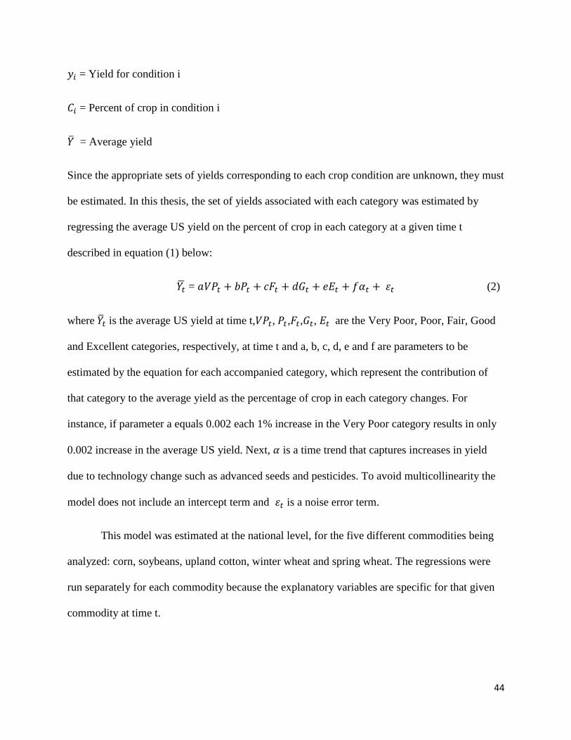
44

𝑦𝑖 = Yield for condition i

𝐶𝑖 = Percent of crop in condition i

�̅� = Average yield

Since the appropriate sets of yields corresponding to each crop condition are unknown, they must

be estimated. In this thesis, the set of yields associated with each category was estimated by

regressing the average US yield on the percent of crop in each category at a given time t

described in equation (1) below:

𝑌�̅� = 𝑎𝑉𝑃𝑡 + 𝑏𝑃𝑡 + 𝑐𝐹𝑡 + 𝑑𝐺𝑡 + 𝑒𝐸𝑡 + 𝑓𝛼𝑡 + 𝜀𝑡 (2)

where �̅�𝑡 is the average US yield at time t,𝑉𝑃𝑡, 𝑃𝑡,𝐹𝑡,𝐺𝑡, 𝐸𝑡 are the Very Poor, Poor, Fair, Good

and Excellent categories, respectively, at time t and a, b, c, d, e and f are parameters to be

estimated by the equation for each accompanied category, which represent the contribution of

that category to the average yield as the percentage of crop in each category changes. For

instance, if parameter a equals 0.002 each 1% increase in the Very Poor category results in only

0.002 increase in the average US yield. Next, 𝛼 is a time trend that captures increases in yield

due to technology change such as advanced seeds and pesticides. To avoid multicollinearity the

model does not include an intercept term and 𝜀𝑡 is a noise error term.

This model was estimated at the national level, for the five different commodities being

analyzed: corn, soybeans, upland cotton, winter wheat and spring wheat. The regressions were

run separately for each commodity because the explanatory variables are specific for that given

commodity at time t.

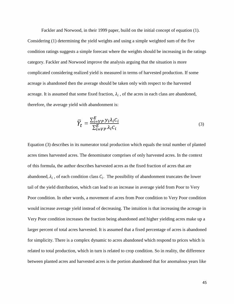
45

Fackler and Norwood, in their 1999 paper, build on the initial concept of equation (1).

Considering (1) determining the yield weights and using a simple weighted sum of the five

condition ratings suggests a simple forecast where the weights should be increasing in the ratings

category. Fackler and Norwood improve the analysis arguing that the situation is more

complicated considering realized yield is measured in terms of harvested production. If some

acreage is abandoned then the average should be taken only with respect to the harvested

acreage. It is assumed that some fixed fraction, 𝜆𝑖 , of the acres in each class are abandoned,

therefore, the average yield with abandonment is:

�̅�𝑡 = ∑ 𝑦𝑖

𝐸𝑖=𝑉𝑃 𝜆𝑖𝐶𝑖

∑ 𝜆𝑖𝐶𝑖𝐸𝑖=𝑉𝑃

(3)

Equation (3) describes in its numerator total production which equals the total number of planted

acres times harvested acres. The denominator comprises of only harvested acres. In the context

of this formula, the author describes harvested acres as the fixed fraction of acres that are

abandoned, 𝜆𝑖 , of each condition class 𝐶𝑖. The possibility of abandonment truncates the lower

tail of the yield distribution, which can lead to an increase in average yield from Poor to Very

Poor condition. In other words, a movement of acres from Poor condition to Very Poor condition

would increase average yield instead of decreasing. The intuition is that increasing the acreage in

Very Poor condition increases the fraction being abandoned and higher yielding acres make up a

larger percent of total acres harvested. It is assumed that a fixed percentage of acres is abandoned

for simplicity. There is a complex dynamic to acres abandoned which respond to prices which is

related to total production, which in turn is related to crop condition. So in reality, the difference

between planted acres and harvested acres is the portion abandoned that for anomalous years like

46

the 2012 drought year when a significant portion of the crops is rated Very Poor it is not the case

the all the acres in Very Poor condition will be abandoned.

The second model in this thesis follows Fackler and Norwood ideas assuming the Very

Poor category is considered abandoned acres described in the equation below:

𝑌�̅� = 𝑏𝑃𝑡 + 𝑐𝐹𝑡 + 𝑑𝐺𝑡 + 𝑒𝐸𝑡 + 𝑓𝛼𝑡 + 𝜀𝑡 (4)

Where the equation description is the same as (1) only excluding the Very Poor category. In

equation (4) if

b = 0, c = 0 and d = e,

Then we can derive the third and last model described in this thesis:

𝑌�̅� = 𝛽 + 𝑎(𝐺 + 𝐸)𝑡 + 𝑏𝛼𝑡 + 𝜀𝑡 (5)

Where 𝑌�̅� is the average US yield at time t, 𝛽 is an intercept, G + E is the sum of the Good and

Excellent categories at time t, 𝛼𝑡 is a specific time trend that captures technology change at time

t, a and b are parameters to be estimated by the regression, and 𝜀𝑡 is an error term. The sum of

Good and Excellent categories is a common approach used by market analysts, traders, and

previous studies as a proxy for overall health of the crops since the Good condition means

prospect for normal yields and the Excellent condition means above average yields (e.g. Irwin,

Good, and Tannura, 2009).

Since the yields are interpreted in this thesis as average yields in each condition class, the

weights should not change over the season. Furthermore, a major modification done in this thesis

unlike Fackler and Norwood, is that all the models were estimated using only the last

observation. Ratings in the beginning of the season are biased towards the Good and Excellent

47

categories because crops conserve all their yield potential. As the growing season progresses,

events such as bad weather and diseases move acres between categories. Since the ratings in each

category reflect the information about these events the last week in the growing season is

assumed to be the only true non-biased observation.

4.3 Results for Corn

Results of the three different models for corn on the national level are displayed on Table

6. As expected, since the first two models are regressions through the origin the R-squared is

close to 1, at 99% for both Model 1 and 2. Model 3 presents an R-squared of 95%, meaning 95%

of the variation in average corn yield at the national level can be explained by changes in the

percentage of the corn crop in Good and Excellent condition. To make a cross-model comparison

between the three models, one needs to look at the improvements in the standard errors. The

standard errors at the national level for corn are 4.2 bushels per acre for Model 1 and 2 and 4.6

bushels per acre for Model 3, which accurately reflects the model’s R-squared statistic.

Considering the Good and Excellent model the base model, one can see that there is only a slight

improvement from the base model compared to the models that include more explanatory

variables. Also as expected, the F-stats are very high for Model 1 and 2. Model 3 also presents a

highly significant F-stats at the 1% level, indicating that the explanatory variables in the models

fit the data very well.

Moving to the coefficients estimated by the models at the national level, according to

theory for Model 1 and 2, the coefficients should increase moving from the Very Poor category

going to Excellent. As an example of how to interpret the coefficients in the models, we can

analyze the coefficient for the Excellent category in Model 1. A coefficient of 1.78 means that

for every 1% increase in the Excellent category there is 1.78 bushel per acre increase in average

48

yield of corn at the national level. Model 1 agrees with theory while Model 2 does not. In Model

2 the coefficient for the Poor category contributes more to average yield than the Fair category.

The interpretation of Model 3’s coefficient is the same as the other two models. In this case, for

every 1% increase in the sum of Good and Excellent categories there is a 0.72 bushel per acre

increase in average yield of corn at the national level. These estimates have notable meaning

both statistically and in a practical sense. For instance, if 90% of the corn crop is rated Excellent

it translates to 160.2 bushels per acre in Model 1. If the remainder 10% is rated Good, according

to Table 1 Model 1, it means another 10.6 bushels per acre totaling 170.8 bushels per acre

average US yield plus a trend increase depending on the year that one is referring to.

The trend variable is always significant for corn for the three models. At the national

level, in Model 3 for instance, a coefficient of 2.06 means that on average the technology change

contributes 2.06 bushels per acre increase to corn yield at the national level every year. In other

words, considering a linear model where 1986 is year 1, by 2006, year 21, technology change

alone would have contributed an increase of 43.3 bushels per acre to corn yield at the national

level on average.

4.4 Results for Soybeans

Table 7 presents the national results of soybeans. Contrary to what theory suggests,

Model 1 coefficients do not increase from Very Poor to Excellent category. The Very Poor

category is the second highest contributing category right after Excellent. Besides the Poor

category, all coefficients are statistically significant. Model 2’s Poor category contributes more

than the Fair category, yet the parameters estimated are increasing from Good to Excellent

category. To illustrate the meaning of parameters in the case of soybeans, taking Model 2’s Good

category’s coefficient of 0.37 and Excellent category’s coefficient of 0.50 suppose the

49

percentages are 75% and 25%, respectively it translates to 40.25 bushels per acre average US

yield of soybeans. Model 3 shows that a 1% increase in the Good and Excellent categories

results in an increase of 0.19 bushels per acre US average yield. As one can see, all parameters

are statistically and practically significant for all models 1, 2, and 3.

At the national level, as expected the R-squared for both Model 1 and 2 are at 99%.

Model 3 has an R-square of 94%. The F-stats is also highly significant at the 1% level for the 3

models. The Root Mean Square Error (RMSE) is 1.10, 1.21 and 1.13 bushels per acre for Model

1, 2 and 3, respectively and even more than the case in corn there is barely an improvement in

Model 1 compared to the base model, Model 3, which is the sum of Good and Excellent

categories. The RMSE is consistent with the model’s fit and F-statistic. Like corn, the trend

variable, as expected, is always significant at the national level for soybeans given its technology

improvement over the years. Technology change contributes 0.41, 042, and 0.43 bushels per acre

increase for Model 1, 2 and 3, respectively every year.

4.5 Results for Upland Cotton

Results for cotton are shown on Table 8. Just like the other three commodities already

discussed in this chapter, Model 1 and 2 R-squared are at 99%. Model 3’s R-squared is 79%,

meaning that 79% of the variation in US average yield of upland cotton is explained by the

model. The RMSE of the three models for a cross- model comparison range from 40 to 45

pounds per acre, also denoting a slight improvement from the base model compared to the other

two models. The RMSE is consistent with their R-squared and F-stats. The F-stats for all three

models is also highly significant at the 1% level.

50

All coefficients for the three different models are statistically significant expect for

Model 1’s Poor category. Model 1’s coefficients are increasing from Poor to Excellent category.

The Very Poor category is the exception for Model 1 with a coefficient of 10.54 pounds per acre

right behind the Excellent category’s coefficient of 10.63. Model 2’s coefficients are also

increasing from Fair to Excellent, except for the Poor category that contributes 5.29 pounds per

acre, which is a little more than 4.09 pounds per acre increase of the Fair category. To put these

coefficients in context, take Model 3’s coefficient of 3.77, meaning that for every 1% increase in

the sum of Good and Excellent categories there is an increase of 3.77 pounds per acre in average

cotton yield at the national level.

Lastly, the trend variable is also significant at the 1% level contributing 9 pounds per acre

for Model 1, 10.33 pounds per acre for Model 2, and 9.96 pounds per acre for Model 3 every

year.

4.6 Results for Winter Wheat

Winter wheat results at the national level are displayed on Table 9. Like the other

commodities, the R-squared for Model 1 and 2 is very high, also at 99%, given it is a regression

through the origin. Model 3’s R-squared is 74%, meaning 74% of the variation on average winter

wheat yield at the national level is explained by the model. The RMSE of the three models for a

cross-model comparison also barely shows an improvement comparing Model 1 1.98 bushels per

acre to Model 3, the base model, 2.04 bushels per acre, even slightly decreasing for Model 2 at

2.14 bushels per acre. The RMSE is consistent with their R-squared and F-stats. The F-stat for all

three models is highly significant at the 1% level, as expected, proving that the independent

variables of the models are effective in explaining average US yield.

51

Compared to the other commodities, Model 3’s lower fit could be associated with the fact

that wheat yield is much more volatile than corn and soybean yields. This high yield volatility is

usually associated with the different nature of the plant’s physiology and different growth

conditions in the states wheat is grown compared to corn and soybeans. Bad weather events such

as hail is said to highly impact wheat yield.

Model 1 and Model 2’s parameters violate the theory of increasing parameters from Very

Poor to Excellent categories as one can observe from Table 9. All parameters are statistically

significant for Model 1 to 3, except the coefficient of Fair category for both Model 1 and 2. As

an example of the practical significance of the models’ parameters, take Model 2 coefficients for

the Good and Excellent categories of 0.56 and 0.39, respectively. If 60% of the winter wheat

crop is rated Good and 40% is rated Excellent, it translates to 49.2 bushels per acre US average

yield of winter wheat.

Finally, even though technology improvements for wheat have been developed at a much

slower pace than corn and soybeans all trend variables are statistically significant at the 1% level.

Trend coefficients are 0.32 bushels per acre for Model 1, 0.34 bushels per acre for Model 2, and

0.37 bushels per acre for Model 3 increase every year.

4.7 Results for Spring Wheat

Spring wheat results are shown in Table 10. R-squared is the same for Model 1 and 2 at

99% since it is a regression through the origin. Model 3’s R-squared is 84%, meaning that 84%

of the variation in average US spring wheat yield can be explained by changes in the percentage

of spring wheat’s crop conditions. For a cross-model comparison, there is not an improvement

from the base model, Model 3 compared to Model 1, since the RMSE remains at 2.6 bushels per

52

acre and Model 2’s RMSE only decreases to 2.58 bushels per acre. Their RMSE is consistent

with their R-squared and F-stats, which is also highly significant at the 1% level.

Agreeing with theory, Model 1’s parameters are increasing from Very Poor to Excellent

Category but the Very Poor and Poor category parameters are not statistically significant. On the

other hand, for Model 2 every 1% increase in the Poor category contributes 0.27 bushels per acre

increase in US yield while the Fair category only contributes 0.20 bushels per acre increase. The

sum of Good and Excellent in Model 3 gives a parameter of 0.24 bushels per acre. The trend

variable is also significant at the 1% level contributing 0.32 bushels per acre for Model 1 and 3

and 0.38 bushels per acre for Model 2 every year.

4.8 Summary

Three statistical models were derived in this chapter. The first model, includes all

categories Very Poor, Poor, Fair, Good and Excellent, a trend variable, and no intercept to avoid

multicollinearity. The second model excludes the Very Poor category following the idea of

abandoned acres by Fackler and Norwood. Lastly, the third model is the sum of Good and

Excellent categories, a trend variable, and an intercept derived from imposed restrictions in the

first two models and it is considered the base model. The three models present a trade-off

between the Principle of Parsimony and amount of information provided by inclusion of more

explanatory variables. All three models will be exercised to forecast crop yield. The next chapter,

chapter 5, presents the forecasted results.

Results from the three different models and five different commodities, corn, soybeans,

upland cotton, winter and spring wheat, were also examined in this chapter. Model 1, which

comprises all 5 categories and Model 2, which comprises of all categories but Very Poor

53

produced similar results. Corn and Soybeans show even more similarities given that both

commodities are grown mainly in the same states and technology improvements developed in a

similar fashion for both commodities. Model 3, which is the sum of Good and Excellent

categories, a trend variable, and intercept had similar fit for corn and soybeans, lower but still

satisfactory fit for upland cotton, spring and winter wheat demonstrating the propensity of these

commodities’ yields to be more volatile to adverse events such as bad weather.

For all commodities in terms of explanatory power, considering Model 1 and 2 are

regressions through the origin14 it will always result in a high R-squared that is not comparable

with the third model, the sum of Good and Excellent categories, R-squared given that the latter

includes an intercept. To make a cross-model comparison, one needs to compare the standard

errors between the models instead, which for all commodities analyzed barely shows an

improvement.

The R-squared of Model 3 ranges from 0.75 for winter wheat to 0.95 for corn. In terms

of parameters, the three models showed practical significance and almost every parameter

showed statistical significance at 1% level and very few at the 5% level as expressed by their

standard errors magnitude compared to the coefficients estimated denoting that indeed crop

condition ratings do explain variation in average US yield and could potentially be used as an

alternative to forecast yield.

Lastly, for model 1 and 2 parameters estimated are expected to be increasing from Very

Poor to Excellent categories. Except for corn and spring wheat’s model 1, the other commodities

14 When the intercept is left off and it does not have a true zero effect, the total sum of squares being modelled is increased, which inflates both SSmodel and SSresidual; however, SSmodel increases relatively more than SSresidual leading to the increase in R2 values.

54

and model 2 generally do not show increasing parameters for all five categories, especially for

the Very Poor and Poor categories. This finding in the data indicates that crop condition analysts

might have difficulty accessing how the much of the crop should be put in those categories and

how the crop will be affected when events that adversely affect yield happen through the

growing season. The sum of Good and Excellent categories, which is the base model, where

yield prospects are normal and above normal should contain enough information to be used as

independent variables in a forecasting model, in other words, model 3.

55

5. A YIELD FORECASTING COMPETITION

5.1 Introduction

The main purpose of the models described in this thesis is their evaluation in terms of

their predictive power. In other words, this chapter aims in answering the question of how well

do the models forecast yield? This chapter describes true forecasts given that the evaluations are

made out of sample.

One of the most important worldwide publications about key agricultural numbers is the

World Agricultural Supply and Demand Estimates (WASDE) by the USDA. The report provides

forecasts and past data about production, stocks, price, yield, and any other information included

in agricultural balance sheets for mostly every existent crop for the US and other countries. The

WASDE is the benchmark forecast used in this chapter. The models developed in this thesis will

be used as an alternative to the WASDE forecasts and will be evaluated based on different

criteria.

5.2 Development of the Yield Prediction Competition

This thesis has adopted a conventional recursive forecasting model. Forecasts were

produced weekly during the growing season of crops that crop condition ratings were available

for each commodity from 2006 to 2015.

5.2.1 Original Crop Condition Ratings

The available sample period for this thesis runs from 1986 to 2015 for all the different

five commodities evaluated. The in-sample period is set initially from 1986 to 2005. Parameters

were estimated using only the last observation (last week) of each year to forecast every week of

56

2006 for all three different models. For the subsequent years, same method is applied: to forecast

every week in 2007, the parameters from the regression of 1986 to 2006 are used and only the

last observation of each year, so on and so forth. Since the growing season varies from year to

year, a given forecasted week is included in the analysis if that week is consistent during the 10

years analyzed. In other words, if the NASS published ratings for a given week in 2006 but not

for 2008, given differences in the start and end of the growing season, that week will be excluded

from the analysis. In this case, the ratings used are the ones obtained from NASS’ data.

5.2.2 Bias Adjustment

The original ratings for each category were bias adjusted to be evaluated against the

original data. It is believed that only the last week of each year is nonbiased. Every other week

was bias adjusted. This process was done in the following fashion, suppose May 21 Good

category has a rating of 50 in 2008. The last week of 2008 is week 40 where the Good category

has a rating of 65. The difference would then be 15 for the Good category in 2008. This

procedure is repeated for each year in the sample creating a series of differences in each

category. Next, the mean of the differences is computed considering the mean is a representative

number of these differences as explained in detail on Chapter 3. The mean differences values

were then added to the original data and all the forecast regressions were run in the same fashion

as before using a recursive method.

5.2.3 Production Weights

A new national data set was created using each state’s original ratings to account for

yield variability between states considering the USDA uses prior year planted acres. The idea is

to make one acre in a high yield soil to weigh more than one acre in a lower yield soil. For

57

instance, for corn one acre in Iowa should weigh more than one acre in North Dakota. To bring

each state’s ratings to a national rating, as mentioned above, the USDA weighs each state’s

ratings by the previous year’s planted acres of every state included in the report for a given

commodity. Also as mentioned above, to account for yield variability between states in this

thesis the weighing was done by state’s production instead of planted acres. The 3-year moving

average and the 5-year moving average of production was calculated for each state included in

the report to weigh the state ratings into new national ratings. A moving average was employed

to smooth out the weights into a more representative number than just the previous year’s

production. The models were run in the same fashion as before using a recursive method. Lastly,

this new national ratings data set was also adjusted for bias and then re-calculated.

5.3 Evaluation Standards

Forecasting accuracy is measured in terms of forecast errors i.e. the difference between

actual yield 𝑦𝑖 and predicted yield 𝑦�̂�. Two evaluation standards were adopted in this thesis. First,

the Root Mean Squared Percentage Error (RMSPE) is used to compare models with different

units. The results are reported in percentage terms and provide a non-linear magnitude of

forecast errors, in other words, bigger errors weight more in the average than smaller errors.

Mathematically, the RMSPE is described as

𝑅𝑀𝑆𝑃𝐸 = √1

𝑛∑ (100 ×

𝑦𝑖 − 𝑦�̂�

𝑦𝑖𝑖)2

where n is the number of forecasts observations. The second measure is the Mean Absolute

Percentage Error (MAPE) which is simply the average of forecast errors without considering

58

their direction also expressed in percentage terms. Unlike the RMSPE, the MAPE provides a

linear error measure, meaning errors weigh the same in the average. It is defined as

𝑀𝐴𝑃𝐸 =1

𝑛 ∑ |100 ×

𝑦𝑖 − 𝑦�̂�

𝑦𝑖|

𝑖

5.4 Forecasting Results

In Chapter 4 and 5, three statistical models that use the entire sample period were

discussed in detail. This chapter discussed the different methods used during the forecasted

period 2006-2015. This thesis has 3 different models, the first model includes all categories,

trend, and no intercept. The second model excludes the Very Poor category, has a trend, and no

intercept. The third and last model is the sum of Good and Excellent, trend and intercept. All

forecasts for the three models used a recursive method and were done in six different ways i.e.

USDA’s original data, bias adjusted, 3-year moving average production weights, 5-year moving

average production weights, 3-year moving average bias adjusted production weights, and lastly,

5-year moving average bias adjusted production weights resulting in 18 different error

comparisons. First, the results that this section discusses are displayed on separate tables of

MAPE and RMSPE for each commodity comparing the 18 different forecasts. The sum of Good

and Excellent categories USDA’s original ratings is established as the base model then each of

the alternative models are compared to the base model, expressed as a ratio, to see how much

improvement the alternative model provides compared to the base model. A ratio bigger than one

means that the base model is a better forecast than the alternative, logically, a ratio smaller than

one will give the magnitude of the forecast improvement provided by the alternative forecast.

Secondly, the MAPE and RMSPE comparison with WASDE is made for each individual

commodity using the best performing model for the week of the WASDE release each year. A

59

composite forecast which is simply the average of the two forecasts’ errors is also shown on the

tables.

5.4.1 Corn Yield Forecasts Results Model Comparison

Table 11 presents out-of-sample MAPE forecasting accuracy statistics for the 18 corn

forecasted models for the 2006 to 2015 forecasted period. The smallest MAPE error of a model

and data set for a given week is highlighted in yellow. For weeks 22 to 25, June 30, and total

average, the model that gives the lower MAPE is the sum of Good and Excellent categories 3-

year moving average bias adjusted production weights. For the weeks 26 to 28, the model that

gives the lower MAPE is all categories 3-year moving average bias adjusted production weights.

For weeks 30 to 34, 36, 37, and 39 the best performing model is less Very Poor category 3-year

moving average production weights. September 15’s best performing model is the less Very Poor

category USDA’s original data. Lastly, September 1’s best performing model is the less Very

Poor category 5-year moving average production weights.

In terms of magnitude, errors should be decreasing as the growing season progresses and

the crop gets closer to being harvested. The best performing model’s errors ranges from 6.4% on

June 2 to 2.76% on September 29. As mentioned before, the model that gives the smallest

average MAPE of 3.92% is the sum of Good and Excellent categories 3-year moving average

bias adjusted production weights.

Table 12 presents the ratio of each model’s forecast statistics compared to the base

model, which is the sum of Good and Excellent categories that uses USDA’s original ratings. A

ratio lower than 1 means that the competing model performs better than the base model.

Logically, a ratio higher than 1 means that the competing model is inferior to the base model. In

60

the same fashion as before, the smallest ratio for a given model during a given week is

highlighted in yellow. The best performing model’s ratio ranges from 0.854 on September 29 to

0.641 on August 11. The model that gives the smallest average MAPE ratio of 0.811 is the less

Very Poor category 3-year moving average production weights.

In the same fashion as before, table 13 presents out-of-sample RMSPE forecasting

accuracy statistics for the 18 corn forecasted models for the 2006 to 2015 period with the

smallest error highlighted in yellow. From June 2 to July 21, the best performing model is all

categories 3-year moving average bias adjusted. The best performing model for July 28 to

August 25 and September 8 to September 29 including the average is the less Very Poor category

3-year moving average production weights. Lastly, only for September 1 the best performing

model is the less Very Poor category 5-year moving average production weights. In terms of

magnitude, the RMSPE ranges from 9.9% on June 2 to 2.9% on September 8. The smallest

average RMSPE is 5.48% for the less Very Poor category 3-year moving average production

weights.

Table 14 also displays the ratio of the competing model to the base model. The best

performing model’s ratio ranges from 0.750 on June 2 to 0.598 on June 30. The model that gives

the smallest average RMSPE ratio of 0.747 is the less Very Poor category 3-year moving average

production weights.

In summary, results show that overall the best model for corn is the sum of Good and

Excellent categories showing an improvement of almost 20% compared to the base model. Corn

forecasts also show to be very responsive to the production weights biased and non-biased

adjusted. A possible reason for corn to be responsive to this weighing method is that states that

produce corn have a wide range of yield variability. Bias adjustments also suit corn well given

61

that the crop recovers little from adverse events that affect yield if it hits during the pollination

period.

5.4.2 Corn Yield Forecasts Results Best Performing Model vs. WASDE

The best performing model in the week of the WASDE release for a given year was

compared to the WASDE forecast error on tables 31 for MAPE and table 32 for RMSPE. The

best performing model for each month is specified in a footnote for each table. Compared to the

WASDE, the models outperformed the USDA, which is the benchmark being used, for the trend-

yield forecast months of June and July for both MAPE and RMSPE. The MAPE for June is 6.1%

compared to 6.5%, while July improves to 4.1% MAPE compared to 4.9%. In terms of RMSPE,

June’s error is 8.8% compared to 11.8% error for the WASDE. July RMSPE is 5.3% compared

to 7.3%. The models failed to outperform WASDE forecasts during the survey yield forecast

months of August and September. However, the MAPE error for August is only 0.3% inferior to

WASDE and RMSPE is only 0.5% inferior to the WASDE. In September, MAPE is 0.6% worse

than WASDE and RMSPE is 0.3% worse than the WASDE.

Forecasts for both the WASDE and the best performing model increases dramatically as

the growing season progresses. The MAPE WASDE forecast improves from 6.5% in June to

1.8% in September, while the best performing model’s forecast improves from 6.1% in June to

2.4% in September. Same dramatically improvement is seem for RMSPE. Lastly, the composite

forecast gives an average error in between the two errors since the composite is an average of the

two ranging from 6.3% in June to 2.1% in August.

62

5.4.3 Soybean Yield Forecasts Results Model Comparison

Table 15 presents out-of-sample MAPE forecasting accuracy statistics for the 18

soybeans’ forecasted models for the 2006 to 2015 forecasted period. In the case of soybeans, the

best performing model for the majority of the weeks is all categories bias adjusted data. The best

performing model error’s range from 3.52% on July 28 to 2.17% on September 29. The smallest

average MAPE is of 2.9% for all categories model bias adjusted data. Table 16 shows the ratio of

the competing model to the base model. The best performing model’s ratio ranges from 0.98 on

September 15 to 0.55 on June 23. The model that gives the smallest average MAPE ratio of 0.89

is also all categories model bias adjusted data.

Table 17 shows the RMSPE, which the best performing model is also all categories bias

adjusted data for the majority of the weeks analyzed. The best performing model error’s range

from 4.41% on August 4 to 2.96% on September 22. The smallest average RMSPE is of 3.74%.

Table 18 also shows the RMSPE ratio of competing models compared to the sum of Good and

Excellent categories USDA data base model. The best performing model’s ratio ranges from

0.62 on June 16 to 0.98 on September 15 of the growing season. The lowest average ratio of 0.92

is provided by all the categories model bias adjusted data.

For soybeans, overall the best model also seems to be the sum of Good and Excellent

categories even when the biggest improvement or best performing model comes from all the

categories model bias adjusted data. Unlike corn, the production weights do not show the same

improvement in forecasting indicating that the variability in yield between states is not as high.

Finally, the bias adjustment also shows to be less beneficial for soybeans than corn given that the

plant does present reproduction if events that affect yield hit during the reproductive period.

63

5.4.4 Soybean Yield Forecasts Results Best Performing Model vs. WASDE

Table 33 and 34 show the best performing model and WASDE comparison. Unlike corn,

the soybean yield forecast outperformed WASDE for the survey forecasted yield months of

August and September for both MAPE and RMSPE. In August MAPE and RMSPE are 3.3%

and 4.4% compared to 3.8% and 4.7% WASDE error. According to industry experts who do

crop tours across the country, corn ears are less misleading than counting soybean pods to

estimate yields, hence, once the WASDE starts using the farmer and objective yield survey to

forecast yields these models can outperform their survey forecasts. For the trend-yield forecasts

month of July the MAPE is 0.2% inferior to WASDE and the RMSPE is 0.5% inferior.

In terms of forecast improvement as the growing season progresses the WASDE

performs worse presenting a 3% error in July just to increase to 3.8% in September, while the

best performing model shows improvements from 3.3% in August to 2.5% in September for

MAPE. The RMSPE shows similar results. The composite forecast shows results of 3.1% in

June, increasing to 3.6% in July and then decreasing back to 3.1% in August.

5.4.5 Upland Cotton Yield Forecasts Results Model Comparison

Table 19 presents out-of-sample MAPE forecasting accuracy statistics results. For cotton,

the model that gives the smallest error is the sum of Good and Excellent categories that uses

USDA’s original ratings or is bias adjusted. Upland cotton presents high errors compared to the

other commodities analyzed in this thesis. For the best performing model error’s range from

8.21% on August 4 to 6.13% on October 20. The smallest average error of 7.58% is given by the

sum of Good and Excellent categories model USDA’s original ratings. Table 20 shows the ratio

of the competing model to the base model. Considering that the best forecast is the base model

64

most of the time, the majority of ratios are bigger than 1. The smallest ratios are given by the

sum of Good and Excellent model bias adjusted data ranging from 0.997 to 1.

Table 21 shows the RMSPE, which the best performing model for almost every week

analyzed is also the sum of Good and Excellent USDA’s original ratings. Errors range from

9.52% on August 4 to 7.29% on October 20. The smallest average error of 8.9% is given by the

same model. Table 22 also shows the RMSPE ratio of competing models compared to the sum of

Good and Excellent categories USDA data base model. As it was the case for MAPE, most ratios

are higher than 1 considering the best performing model is the base model, being the smallest

one 0.998. In the case of upland cotton, neither adjusting for bias nor reweighting for production

improved the forecast.

5.4.6 Upland Cotton Yield Forecasts Results Best Performing Model vs. WASDE

Table 35 and 36 show the best performing model and WASDE comparison. In terms of

both MAPE and RMSPE the best performing model failed to outperform WASDE forecasts

showing a much higher error than the WASDE. WASDE MAPE errors range from 5.2% in July

to 5.5% in September, while RMSPE shows errors of 5.8% in July, increasing to 6.4% in August,

and decreasing to 6.2% in September. Curiously, the WASDE has a smaller error forecast for the

trend-yield forecast month of July than the survey months of August and September. One

possible reason for upland cotton to present high errors compared to the other commodities

analyzed and for the WASDE forecast survey-yield months to be slightly inferior to the trend-

yield month is perhaps the nature of the plant in terms of its yield estimation, which relies on

counting squares, blooms, and bolls of the plant while the trend-yield months rely on historical

average weather data.

65

In terms of forecast improvement as the growing season progresses, the WASDE forecast

ranges from 5.2% in July to 5.5% in September denoting that the USDA also has problems

improving their forecast as the growing season progresses even though the forecast method

changes as mentioned above. The best performing model has its best forecast in September

presenting a MAPE of 7.5%. Similar results are seen for RMSPE. Lastly, the composite forecast

is particularly important in the case of upland cotton given its large forecast errors for both the

WASDE and the models developed in this thesis. The composite for July is 6.5%, increasing in

August to 6.7%, and then decreasing in September back to 6.5%.

5.4.7 Winter Wheat Yield Forecasts Results Model Comparison

Table 23 and table 25 present out-of-sample MAPE and RMSPE, respectively forecasting

accuracy statistics for the 18 winter wheat forecasted models for the 2006 to 2015 period.

Winter Wheat’s best performing model for the majority of the weeks for both MAPE and

RMSPE is the less Very Poor Category 3-year moving average production weights bias adjusted

data. The issue of abandoned acres seem to be more important for winter wheat considering that

the less Very Poor gives the smallest error. For MAPE, errors range from 5.12% on May 21 to

4.46% on April 14, while RMSPE range from 5.85% on May 21 to 4.95% also on April 14. The

smallest average is of 4.8% for MAPE and 5.52% for RMSPE also given by the same model.

Next, table 24 and table 26 show the ratio of the competing model to the base model. For MAPE

ratios range from 0.59 on April 28 to 0.82 on June 9. RMSPE’s ratios range from 0.62 on April

14 to 0.80 also on June 9. The smallest average is 0.71 for both MAPE and RMSPE given also

by the same model.

For winter wheat, considering all ratios are smaller than 1, the competing model is always

better than the base model. Considering that there is no distinction between the varieties of

66

winter wheat in the crop conditions the production weights are very important for winter wheat

because it takes into account the yield variability between states. The adjustment for bias is also

very important for winter wheat since the plant is very sensitive to events that affect its yield

through the growing season. Overall, the forecasting models developed for winter wheat show a

dramatic improvement compared to the base model.

5.4.8 Winter Wheat Yield Forecasts Results Best Performing Model vs. WASDE

Table 37 and 38 show the best performing model forecast comparison to WASDE

forecast. In the same fashion as corn, winter wheat’s best performing model outperforms the

WASDE for the trend-yield forecast but not for the survey yield forecast months. MAPE does

not decrease from April to June staying at 4.7% while the WASDE forecast dramatically

improves from 5.2% in April to 2% in June. The RMSPE remains at 5.6% for April and June but

decreases in May to 5.3% indicating that as the USDA adjusts its WASDE forecast it does not

align the crop conditions accordingly. The composite forecast ranges from 5% in April to 3.4%

in June indicating that the composite forecast would be a better option for winter wheat than the

best performing model alone.

5.4.9 Spring Wheat Yield Forecasts Results Model Comparison

Table 27 presents out-of-sample MAPE forecasting accuracy statistics for the 18 corn

forecasted models also for the 2006 to 2015 period. Spring Wheat’s best performing model for

all the weeks during the period analyzed is the sum of Good and Excellent categories USDA’s

original data, which is also the base model. MAPE error ranges from 8.23% on June 9 to 6% on

July 28 averaging 6.76%. Table 28 shows MAPE ratios, as it was the case in upland cotton,

since the best performing model is the base model all ratios are higher than 1 ranging from 1.14

67

on July 28 for the best performing model to 1.022 on July 7 averaging 1.07 for the sum of Good

and Excellent model 3-year moving average production weights.

Table 29 shows RMSPE forecasting accuracy statistic where the best performing model

for the majority of the weeks is also the sum of Good and Excellent but bias adjusted data.

RMSPE ranges from 10.95% on June 9 to 7.28% on August 4 averaging 8.9%. Table 30 presents

the ratio of the competing model to the base model where the ratios range from 0.9 on June 23 to

1.06 on July 28 for the best performing models. The smallest average ratio is of 0.996 for the

sum of Good and Excellent model 3-year moving average production weights.

Spring wheat presents high errors compared to the other commodities. Production

weights and adjustment for bias does not show large forecast improvements for spring wheat.

Possible explanations for this are that spring wheat is only grown in a small geographic area and

most of its acreage comes from the same state, North Dakota, hence production weights, which

account for yield variability between states is not as crucial in this case. A possible explanation

for the bias adjustment not to show a significant improvement in forecasting for spring wheat is

that, spring wheat has the shortest growing period among all commodities, therefore, the need to

adjust other ratings to the last rating of the growing season is small.

5.4.10 Spring Wheat Yield Forecasts Results Best Performing Model vs. WASDE

Tables 39 and 40 display the forecast comparison. In the case of spring wheat, the best

performing model evaluated in terms of MAPE outperforms the WASDE for the survey months

of June and July but fails to outperform the WASDE in August. In terms of RMSPE, the best

performing model fails to outperform the WASDE for all three months of June, July, and

August. However, the RMSPE decreases significantly as the growing season progresses ranging

68

from 10.9% in June to 7.3% in August, while WASDE ranges from 9.8% in June to 6.9% in

August. Even though there is improvements in forecasting over the growing season, both the

WASDE and the best performing model show high errors compared to the other commodities

analyzed. The composite forecast ranges from 8.4% in June to 5.9% in August and as it was the

case in winter wheat the composite forecast presents as a good alternative than the best

performing model alone.

5.5 Summary

The models developed in this thesis beat the WASDE for the trend-yield forecasting

months for most commodities. Given the nature of the method used by the USDA i.e. the

USDA’s uses historical average weather data to forecast yield, it is not surprising that these

models provide a superior forecast. For the survey-yield forecast months, USDA’s forecasts have

proven to be superior also given the method used i.e. the farmer’s list survey and objective yield

survey, except for the case of soybeans where yield prediction from survey is the most

misleading among the five commodities analyzed. The best performing model also beats the

WASDE for two out of three survey yield months for spring wheat.

69

6. Conclusion

6.1 Review

This thesis explored the relationship between US yield and crop condition ratings

published through the growing season of crops by NASS. Previous work that studied yield

estimation and forecasting comprise of four main areas, i.e. agronomy studies, remote sensing

imagery, hybrid studies that include both agronomy studies and remote sensing, and empirical

statistical studies. Agronomists analyze plant physiology and phenology in complex

mathematical models to draw conclusion about crop yields. Remote sensing imagery uses

satellite data to infer crop yields. As an empirical statistical research, this thesis uses crop

condition ratings, which are widely used by market participants as an information tool for the

condition of the crops during the growing season. Crop condition ratings combine information

from weather events, pests and diseases, and large scale coverage of the main crops grown in the

US.

The commodities studied in this thesis are corn, soybean, upland cotton, winter wheat,

and spring wheat yields at the US scale. Three statistical models were studied in detail. The first

model included all crop condition categories Very Poor, Poor, Fair, Good and Excellent, a trend

to capture technology change, and no intercept to avoid multicollinearity. The second model

explained was less the Very Poor category that were considered abandoned acres, a trend, and no

intercept. The last model explained was the sum of the Good and Excellent categories, a trend,

and intercept. This study based its ideas in the work of Kruse and Smith (1994) and Fackler and

Norwood (1999). The period analyzed was 1986 to 2015.

70

The three models developed were run with 6 different data sets to hold a forecasting

competition between the models and the benchmark WASDE. The out-of-sample period

analyzed is 2006 to 2015. The six different data sets include USDA NASS original crop

condition ratings, crop condition ratings adjusted for bias through the growing season, 3-year

moving average production weights, 5-year moving average production weights, 3-year moving

average production weights adjusted for bias, and 5-year moving average production weights

adjusted for bias. The evaluation was based on common error measures of forecasting accuracy

statistics, MAPE and RMSPE, using a recursive method.

6.2 Summary of Findings

Results for all categories model show increasing coefficients from Very Poor to Excellent

category for corn and spring wheat ranging from 0.25 to 1.78 and 0.15 to 0.67, respectively.

Technology change contributes 1.99 and 0.33 bushels per acre yield increase every year for corn

and spring wheat, respectively. All coefficients are also significant at the 1% level except for the

Poor category coefficient that is significant at 5% level and the Very Poor coefficient which does

not show significance for corn. Spring wheat’s coefficients show significance for all coefficients

at the 1% level but the Very Poor and Poor categories. Soybeans and winter wheat do not show

increasing coefficients from Very Poor to Excellent. Soybean’s coefficients are significant at the

1% level, the Very Poor coefficient is significant at the 5% level, and the Poor category does not

show significance. Technology change contributes 0.41 bushels per acre increase in yield of

soybeans every year. Winter wheat’s coefficients are significant at the 1% level, the Very Poor

coefficient is significant at the 5% level, and the Fair category does not show significance.

Technology change contributes 0.32 increase in yield every year. Lastly, upland cotton’s

coefficients are increasing from Fair to Excellent and are significant at the 1% level. The Very

71

Poor category is also significant at 1% but the Poor is not. Technology change contributes 9

pounds per acre yield increase every year.

The less Very Poor category model shows that the Fair category contributes less to yield

than the Poor category for corn, soybean, cotton, and spring wheat. All coefficients show

significance at 1% or 5% level. Technology change contributes 2.05, 0.43, 10.33 and 0.33 yield

increase for corn, soybeans, upland cotton, and spring wheat, respectively. Winter wheat does

not show a clear patter for increasing coefficients from Poor to Excellent. Winter wheat’s

coefficients are significant at the 1% level, the Excellent category coefficient is significant at the

5% level, and the Fair category does not show significance. Technology change contributes 0.34

bushels per acre increase every year.

The sum of Good and Excellent model shows coefficients of 0.72, 0.19, 3.77, 0.18, and

0.25 for corn, soybeans, upland cotton, winter wheat, and spring wheat, respectively. Technology

change contributes 2.07, 0.43, 9.96, 0.38, and 0.38 yield increase every year for corn, soybeans,

upland cotton, winter wheat, and spring wheat, respectively.

The forecasting competition results indicated that the best performing model for corn

compared to the WASDE, release during each year analyzed, for the survey-months yield

forecasting is the less Very Poor category that uses 3-year moving average production weights.

The trend-yield forecasting months’ best performing model is all categories 3-year moving

average bias adjusted production weights except for MAPE in June, which case the model used

was the sum of Good and Excellent 3-year moving average bias adjusted production weights.

Soybean’s best performing model for MAPE is all categories bias adjusted data for July and

August, and USDA’s original data for September. In the case of RMSPE, it is sum of Good and

72

Excellent model bias adjusted for July, and USDA’s original data for September. For the month

of August, just like MAPE, the model is also all categories bias adjusted data.

Cotton’s best performing model is the sum of Good and Excellent that uses USDA’s

original data for RMSPE and the sum of Good and Excellent bias adjusted data for MAPE’s

months of August and September. July’s best performing model was all categories bias adjusted.

Spring wheat’s best performing model was the sum of Good and Excellent in every instance. The

data set used was USDA’s original data for all MAPE’s months and RMSPE’s month of August,

3-year moving average production weights for RMSPE’s July and 3-year moving average bias

adjusted production weights for RMSPE’s June. Finally, winter wheat’s best performing is the

less Very Poor category 3-year moving average bias adjusted production weights for MAPE and

RMSPE’s month of June. For RMSPE’s months of April and May, the best performing model is

all categories bias adjusted data for April and 5-year moving average bias adjusted production

weights for May.

In summary, the models developed in this thesis beat the WASDE for the trend-yield

forecasting months in most instances. The models beat the WASDE for survey- yield forecasting

months for soybeans and spring wheat.

6.3 Future Work and Concluding Remarks

This study assumes that crop condition ratings is fair data to forecast US yield. The

forecast is only as good as the input data. Considering that crop conditions are known to

dramatically change as the growing season progresses, this thesis aimed to 1) understand the

collection and behavior of crop condition ratings to properly understand their strengths and

limitations as a market information tool 2) correct possible bias in the data, and 3) improve their

73

weighing method. By replicating USDA weighing process, this study used a moving average of

production instead of previous year’s planted acres assuming a moving average of production is

a better representation of how much each state should weigh in the ratings than just planted

acres. To put this in context, in the case of corn for instance, this study aimed to make one acre

in Iowa to weigh a little more than one acre in North Dakota considering Iowa’s soil yields more

corn per acre than North Dakota’s soil. For all commodities, by comparing the production-

weighed dataset to the USDA original dataset weighing by production changes the original rating

dramatically in the beginning of the season and for the Fair to Excellent category. As the

growing season progresses the changes in ratings get smaller.

Key findings of this study are 1) if the USDA increases its WASDE yield forecasting

dramatically and does not align crop conditions accordingly the forecast will be poor resulting in

large errors compared to US final yield as it was the case in 2008 and 2015, 2) when weather

becomes an issue these models perform very well compared to WASDE as it was the case in

2012, 3) the models are a good forecast beating the USDA WASDE in almost every instance for

the trend-yield months, 4) almost in every instance the best performing model did not use

USDA’s original ratings, which implies that the corrections made to the data are rational 5)

except for soybeans and spring wheat, the WASDE survey-yield months are a better forecast

than the statistical models developed in this thesis given the nature of the commodities and

USDA’s superior method 6) Weighting by production instead of planted acres becomes

particularly important when there is a wide range of yield variability between states like it is the

case for corn and winter wheat 7) Correction for bias becomes particularly important the more

the crop is sensitive to adverse events that affect yield during its reproduction stage.

74

Compared to the beginning of the season the models present large forecast

improvements. Forecasting models are made to be translated into early price signals for market

participants, these models serve this purpose since they present significant results. By combining

forecasting models or a composite forecasting model, with technical analysis, and values that are

being traded in the physical market (i.e. values traded in the Illinois river- CIF Gulf Market,

processor spot market in key locations) traders could benefit from the insights provided by this

thesis. Finally, this thesis leaves room for future work in the bias correction method and less

Very Poor category model. This thesis considered the mean as a representative number to correct

the ratings while the mean assumes that the condition ratings are normally distributed. As a

robustness check for non-normality one could test the median to correct the ratings. Considering

that the results for the less Very Poor category model compared to the other models only show

modest improvements for most commodities a more accurate method for estimating the portion

of abandoned acres than eliminating the Very Poor category also leaves room for investigation.

Additionally, considering the large forecast errors that upland cotton and spring wheat show to

have compared to the other commodities for both WASDE and the models developed in this

thesis, these two crops also leave room for further investigation. Finally, future work of

forecasting yield on the state level also presents an opportunity for development.

75

FIGURES AND TABLES

Figure 1. Corn- Condition Ratings Mean for Each Category for Years 1986 to 2015,

Beginning, Middle, and End of the Season

Average Date Condition (%)

Very Poor Poor Fair Good Excellent

JUN-2 1 5 28 55 12

JUN-28 4 9 24 47 17

SEP-29 4 9 24 47 16

0

10

20

30

40

50

60

JUN-2 JUN-28 SEP-29

Very Poor Poor Fair Good Excellent

76

Figure 2. Soybeans- Condition Ratings Mean for Each Category for Years 1986 to 2015,

Beginning, Middle, and End of the Season

Average Date Condition (%)

Very Poor Poor Fair Good Excellent

JUN-16 1 6 31 53 9

AUG-4 3 10 29 46 12

SEP-29 4 10 29 45 12

0

10

20

30

40

50

60

JUN-16 AUG-4 SEP-29

Very Poor Poor Fair Good Excellent

77

Figure 3. Cotton, Upland- Condition Ratings Mean for Each Category for Years 1986 to

2015, Beginning, Middle, and End of the Season

Average Date Condition (%)

Very Poor Poor Fair Good Excellent

JUN-16 5 10 34 43 8

AUG-4 5 10 32 43 10

SEP-29 6 12 34 39 9

0

5

10

15

20

25

30

35

40

45

50

JUN-16 AUG-4 SEP-29

Very Poor Poor Fair Good Excellent

78

Figure 4. Winter Wheat- Condition Ratings Mean for Each Category for Years 1986 to

2015, Beginning, Middle, and End of the Season

Average Date Condition (%)

Very Poor Poor Fair Good Excellent

APR-7 6 11 31 43 10 MAY-19 8 13 30 39 9 JUN-23 9 14 31 37 9

0

5

10

15

20

25

30

35

40

45

50

APR-7 MAY-19 JUN-23

Very Poor Poor Fair Good Excellent

79

Figure 5. Spring Wheat- Condition Ratings Mean for Each Category for Years 1986 to

2015, Beginning, Middle, and End of the Season

Average Date Condition (%)

Very Poor Poor Fair Good Excellent

JUN-9 2 5 23 59 11 JUL-7 3 8 24 53 12 AUG-4 3 8 28 50 10

0

10

20

30

40

50

60

70

JUN-9 JUL-7 AUG-4

Very Poor Poor Fair Good Excellent

80

Table 1. Corn- Mean and St. Deviation Difference between the last week and other week’s

ratings during the year per category

VERY POOR CATEGORY Average Mean St. Dev. Number of

T-value p-value Date Difference Difference Observations Jun-2 3.45 4.85 29.00 3.83 0.001 * Jun-9 3.45 4.75 29.00 3.91 0.001 * Jun-16 3.10 4.69 30.00 3.62 0.001 * Jun-23 2.93 4.26 30.00 3.77 0.001 * Jun-30 2.52 3.83 29.00 3.54 0.001 * Jul-7 1.73 3.31 30.00 2.87 0.008 * Jul-14 1.27 2.77 30.00 2.51 0.018 * Jul-21 0.90 1.52 30.00 3.25 0.003 * Jul-28 0.53 1.48 30.00 1.97 0.058 Aug-4 -0.03 1.71 30.00 -0.11 0.458 Aug-11 -0.33 1.42 30.00 -1.28 0.105 Aug-18 -0.40 1.07 30.00 -2.05 0.025 * Aug-25 -0.37 0.76 30.00 -2.63 0.007 * Sep-1 -0.37 0.96 30.00 -2.08 0.023 * Sep-8 -0.53 0.97 30.00 -3.00 0.003 * Sep-15 -0.45 0.95 29.00 -2.55 0.008 * Sep-22 -0.41 0.73 29.00 -3.04 0.003 * Sep-29 -0.21 0.56 29.00 -1.99 0.028 * Note: asterisk denotes significance at the 5% level

POOR CATEGORY Average Mean St. Dev. Number of

T-value p-value

Date Difference Difference Observations

Jun-2 4.69 6.43 29.00 3.93 0.001 * Jun-9 4.24 5.98 29.00 3.82 0.001 * Jun-16 3.83 5.05 30.00 4.16 0.000 * Jun-23 3.23 4.00 30.00 4.43 0.000 * Jun-30 2.93 3.30 30.00 4.87 0.000 * Jul-7 1.97 2.82 30.00 3.82 0.001 * Jul-14 1.47 2.15 30.00 3.74 0.001 * Jul-21 0.97 1.88 30.00 2.81 0.009 * Jul-28 0.47 1.74 30.00 1.47 0.152 Aug-4 -0.07 2.12 30.00 -0.17 0.432 Aug-11 -0.43 2.05 30.00 -1.16 0.128 Aug-18 -0.70 1.82 30.00 -2.10 0.022 * Aug-25 -0.57 1.65 30.00 -1.88 0.035 * Sep-1 -0.97 1.56 30.00 -3.38 0.001 * Sep-8 -0.87 1.46 30.00 -3.26 0.001 * Sep-15 -0.66 1.45 29.00 -2.44 0.011 * Sep-22 -0.66 1.11 29.00 -3.18 0.002 * Sep-29 -0.34 0.90 29.00 -2.07 0.024 * Note: asterisk denotes significance at the 5% level

81

Table 1. (cont.)

FAIR CATEGORY Average Mean St. Dev. Number of

T-value p-value

Date Difference Difference Observations

Jun-2 -4.00 8.55 29.00 -2.52 0.009 * Jun-9 -3.38 8.38 29.00 -2.17 0.019 * Jun-16 -2.07 6.89 30.00 -1.64 0.056 Jun-23 -1.47 6.65 30.00 -1.21 0.118 Jun-30 -0.30 6.59 30.00 -0.25 0.402 Jul-7 -0.07 6.27 30.00 -0.06 0.477 Jul-14 0.43 4.75 30.00 0.50 0.621 Jul-21 0.53 3.29 30.00 0.89 0.382 Jul-28 0.70 3.08 30.00 1.25 0.223 Aug-4 0.90 3.20 30.00 1.54 0.134 Aug-11 0.47 3.32 30.00 0.77 0.447 Aug-18 0.37 3.15 30.00 0.64 0.528 Aug-25 -0.30 2.83 30.00 -0.58 0.283 Sep-1 -0.53 2.45 30.00 -1.19 0.121 Sep-8 -0.53 1.89 30.00 -1.55 0.066 Sep-15 -0.86 1.57 29.00 -2.95 0.003 * Sep-22 -0.72 1.25 29.00 -3.12 0.002 * Sep-29 -0.34 1.17 29.00 -1.58 0.062 Note: asterisk denotes significance at the 5% level

GOOD CATEGORY Average Mean St. Dev. Number of

T-value p-value

Date Difference Difference Observations

Jun-2 -8.86 10.62 29.00 -4.49 0.000 * Jun-9 -8.48 9.75 29.00 -4.69 0.000 * Jun-16 -8.00 7.61 30.00 -5.76 0.000 * Jun-23 -6.60 6.30 30.00 -5.74 0.000 * Jun-30 -5.50 5.57 30.00 -5.41 0.000 * Jul-7 -3.70 5.58 30.00 -3.63 0.001 * Jul-14 -2.63 4.19 30.00 -3.44 0.001 * Jul-21 -1.27 3.55 30.00 -1.95 0.030 * Jul-28 -0.67 3.70 30.00 -0.99 0.166 Aug-4 0.17 3.39 30.00 0.27 0.790 Aug-11 0.77 3.73 30.00 1.13 0.269 Aug-18 0.93 3.38 30.00 1.51 0.142 Aug-25 0.87 3.22 30.00 1.47 0.152 Sep-1 0.97 2.67 30.00 1.98 0.057 Sep-8 0.53 2.70 30.00 1.08 0.288 Sep-15 0.45 2.46 29.00 0.98 0.334 Sep-22 0.48 2.03 29.00 1.28 0.211 Sep-29 -0.10 2.11 29.00 -0.26 0.397 Note: asterisk denotes significance at the 5% level

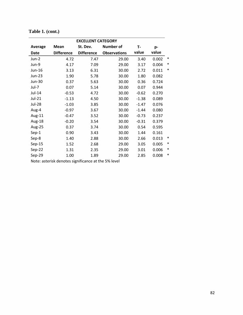
82

Table 1. (cont.)

EXCELLENT CATEGORY Average Mean St. Dev. Number of T-

value p-

value

Date Difference Difference Observations Jun-2 4.72 7.47 29.00 3.40 0.002 * Jun-9 4.17 7.09 29.00 3.17 0.004 *

Jun-16 3.13 6.31 30.00 2.72 0.011 * Jun-23 1.90 5.78 30.00 1.80 0.082 Jun-30 0.37 5.63 30.00 0.36 0.724 Jul-7 0.07 5.14 30.00 0.07 0.944 Jul-14 -0.53 4.72 30.00 -0.62 0.270 Jul-21 -1.13 4.50 30.00 -1.38 0.089 Jul-28 -1.03 3.85 30.00 -1.47 0.076 Aug-4 -0.97 3.67 30.00 -1.44 0.080 Aug-11 -0.47 3.52 30.00 -0.73 0.237 Aug-18 -0.20 3.54 30.00 -0.31 0.379 Aug-25 0.37 3.74 30.00 0.54 0.595 Sep-1 0.90 3.43 30.00 1.44 0.161 Sep-8 1.40 2.88 30.00 2.66 0.013 * Sep-15 1.52 2.68 29.00 3.05 0.005 * Sep-22 1.31 2.35 29.00 3.01 0.006 *

Sep-29 1.00 1.89 29.00 2.85 0.008 *

Note: asterisk denotes significance at the 5% level

83

Table 2. Soybeans- Mean and St. Deviation Difference between the last week and other

week’s ratings during the year per category

VERY POOR CATEGORY

Average Mean St. Dev. Number of T-value p-value

Date Difference Difference Observations Jun-16 2.96 2.72 26 5.55 0.000 *

Jun-23 2.48 2.72 29 4.91 0.000 *

Jun-30 2.23 2.42 30 5.06 0.000 *

Jul-7 1.73 2.48 30 3.83 0.001 *

Jul-14 1.63 2.04 30 4.38 0.000 *

Jul-21 1.37 1.94 30 3.86 0.001 *

Jul-28 1.10 1.92 30 3.14 0.004 *

Aug-4 0.67 1.88 30 1.94 0.062

Aug-11 0.50 1.76 30 1.56 0.130

Aug-18 0.30 1.62 30 1.01 0.319

Aug-25 0.17 1.29 30 0.71 0.484

Sep-1 0.03 1.00 30 0.18 0.856

Sep-8 -0.10 0.88 30 -0.62 0.270

Sep-15 -0.20 0.81 30 -1.36 0.092

Sep-22 -0.14 0.79 29 -0.94 0.177

Sep-29 -0.10 0.62 29 -0.90 0.187

Note: asterisk denotes significance at the 5% level

POOR CATEGORY Average Mean St. Dev. Number of

T-value p-value Date Difference Difference Observations Jun-16 4.27 3.72 26 5.86 0.000 *

Jun-23 3.62 3.58 29 5.45 0.000 *

Jun-30 3.10 3.40 30 5.00 0.000 *

Jul-7 2.40 3.71 30 3.54 0.001 *

Jul-14 2.07 3.30 30 3.43 0.002 *

Jul-21 1.83 3.52 30 2.85 0.008 *

Jul-28 1.47 3.12 30 2.58 0.015 *

Aug-4 0.53 3.20 30 0.91 0.369

Aug-11 0.43 3.01 30 0.79 0.437

Aug-18 0.07 2.65 30 0.14 0.891

Aug-25 0.20 2.16 30 0.51 0.615

Sep-1 -0.23 1.41 30 -0.91 0.186

Sep-8 -0.47 1.20 30 -2.14 0.021 *

Sep-15 -0.57 1.28 30 -2.43 0.011 *

Sep-22 -0.48 1.09 29 -2.39 0.012 *

Sep-29 -0.31 0.71 29 -2.35 0.013 *

Note: asterisk denotes significance at the 5% level

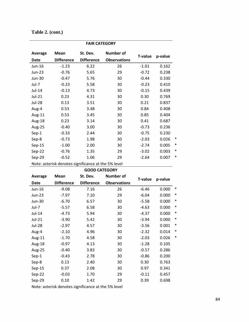
84

Table 2. (cont.)

FAIR CATEGORY

Average Mean St. Dev. Number of T-value p-value

Date Difference Difference Observations Jun-16 -1.23 6.22 26 -1.01 0.162

Jun-23 -0.76 5.65 29 -0.72 0.238

Jun-30 -0.47 5.76 30 -0.44 0.330

Jul-7 -0.23 5.58 30 -0.23 0.410

Jul-14 -0.13 4.73 30 -0.15 0.439

Jul-21 0.23 4.31 30 0.30 0.769

Jul-28 0.13 3.51 30 0.21 0.837

Aug-4 0.53 3.48 30 0.84 0.408

Aug-11 0.53 3.45 30 0.85 0.404

Aug-18 0.23 3.14 30 0.41 0.687

Aug-25 -0.40 3.00 30 -0.73 0.236

Sep-1 -0.33 2.44 30 -0.75 0.230

Sep-8 -0.73 1.98 30 -2.03 0.026 *

Sep-15 -1.00 2.00 30 -2.74 0.005 *

Sep-22 -0.76 1.35 29 -3.02 0.003 *

Sep-29 -0.52 1.06 29 -2.64 0.007 *

Note: asterisk denotes significance at the 5% level

GOOD CATEGORY Average Mean St. Dev. Number of

T-value p-value Date Difference Difference Observations Jun-16 -9.08 7.16 26 -6.46 0.000 *

Jun-23 -7.97 7.10 29 -6.04 0.000 *

Jun-30 -6.70 6.57 30 -5.58 0.000 *

Jul-7 -5.57 6.58 30 -4.63 0.000 *

Jul-14 -4.73 5.94 30 -4.37 0.000 *

Jul-21 -3.90 5.42 30 -3.94 0.000 *

Jul-28 -2.97 4.57 30 -3.56 0.001 *

Aug-4 -2.10 4.96 30 -2.32 0.014 *

Aug-11 -1.70 4.58 30 -2.03 0.026 *

Aug-18 -0.97 4.13 30 -1.28 0.105

Aug-25 -0.40 3.83 30 -0.57 0.286

Sep-1 -0.43 2.78 30 -0.86 0.200

Sep-8 0.13 2.40 30 0.30 0.763

Sep-15 0.37 2.08 30 0.97 0.341

Sep-22 -0.03 1.70 29 -0.11 0.457

Sep-29 0.10 1.42 29 0.39 0.698

Note: asterisk denotes significance at the 5% level

85

Table 2. (cont.)

EXCELLENT CATEGORY Average Mean St. Dev. Number of

T-value p-value Date Difference Difference Observations Jun-16 3.08 4.98 26 3.15 0.004 *

Jun-23 2.62 4.33 29 3.26 0.003 *

Jun-30 1.83 4.56 30 2.20 0.036 *

Jul-7 1.67 4.56 30 2.00 0.055 Jul-14 1.17 4.11 30 1.55 0.131 Jul-21 0.47 3.87 30 0.66 0.514 Jul-28 0.27 3.47 30 0.42 0.677 Aug-4 0.37 3.54 30 0.57 0.575 Aug-11 0.23 3.62 30 0.35 0.726 Aug-18 0.37 3.41 30 0.59 0.560 Aug-25 0.43 3.11 30 0.76 0.452 Sep-1 0.97 2.97 30 1.79 0.085 Sep-8 1.17 2.56 30 2.50 0.019 *

Sep-15 1.40 2.27 30 3.38 0.002 *

Sep-22 1.41 1.82 29 4.18 0.000 *

Sep-29 0.83 1.36 29 3.27 0.003 *

Note: asterisk denotes significance at the 5% level

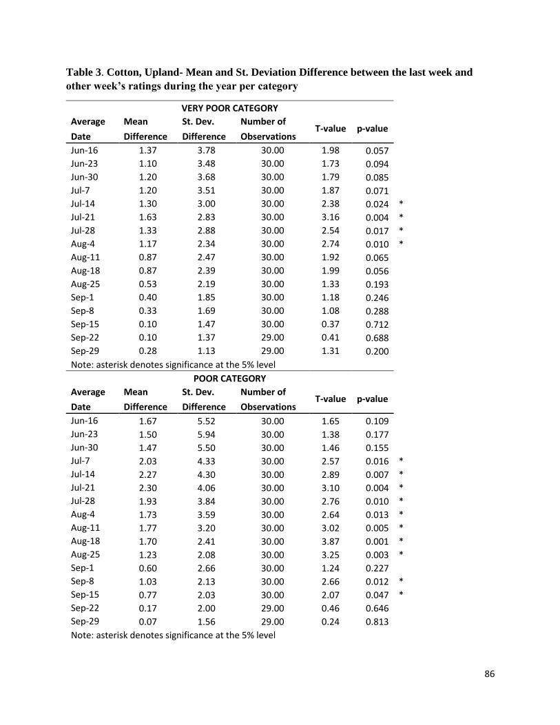
86

Table 3. Cotton, Upland- Mean and St. Deviation Difference between the last week and

other week’s ratings during the year per category

VERY POOR CATEGORY Average Mean St. Dev. Number of

T-value p-value Date Difference Difference Observations Jun-16 1.37 3.78 30.00 1.98 0.057 Jun-23 1.10 3.48 30.00 1.73 0.094 Jun-30 1.20 3.68 30.00 1.79 0.085 Jul-7 1.20 3.51 30.00 1.87 0.071 Jul-14 1.30 3.00 30.00 2.38 0.024 *

Jul-21 1.63 2.83 30.00 3.16 0.004 *

Jul-28 1.33 2.88 30.00 2.54 0.017 *

Aug-4 1.17 2.34 30.00 2.74 0.010 *

Aug-11 0.87 2.47 30.00 1.92 0.065 Aug-18 0.87 2.39 30.00 1.99 0.056 Aug-25 0.53 2.19 30.00 1.33 0.193 Sep-1 0.40 1.85 30.00 1.18 0.246 Sep-8 0.33 1.69 30.00 1.08 0.288 Sep-15 0.10 1.47 30.00 0.37 0.712 Sep-22 0.10 1.37 29.00 0.41 0.688 Sep-29 0.28 1.13 29.00 1.31 0.200 Note: asterisk denotes significance at the 5% level

POOR CATEGORY Average Mean St. Dev. Number of

T-value p-value Date Difference Difference Observations Jun-16 1.67 5.52 30.00 1.65 0.109 Jun-23 1.50 5.94 30.00 1.38 0.177 Jun-30 1.47 5.50 30.00 1.46 0.155 Jul-7 2.03 4.33 30.00 2.57 0.016 *

Jul-14 2.27 4.30 30.00 2.89 0.007 *

Jul-21 2.30 4.06 30.00 3.10 0.004 *

Jul-28 1.93 3.84 30.00 2.76 0.010 *

Aug-4 1.73 3.59 30.00 2.64 0.013 *

Aug-11 1.77 3.20 30.00 3.02 0.005 *

Aug-18 1.70 2.41 30.00 3.87 0.001 *

Aug-25 1.23 2.08 30.00 3.25 0.003 *

Sep-1 0.60 2.66 30.00 1.24 0.227 Sep-8 1.03 2.13 30.00 2.66 0.012 *

Sep-15 0.77 2.03 30.00 2.07 0.047 *

Sep-22 0.17 2.00 29.00 0.46 0.646 Sep-29 0.07 1.56 29.00 0.24 0.813 Note: asterisk denotes significance at the 5% level

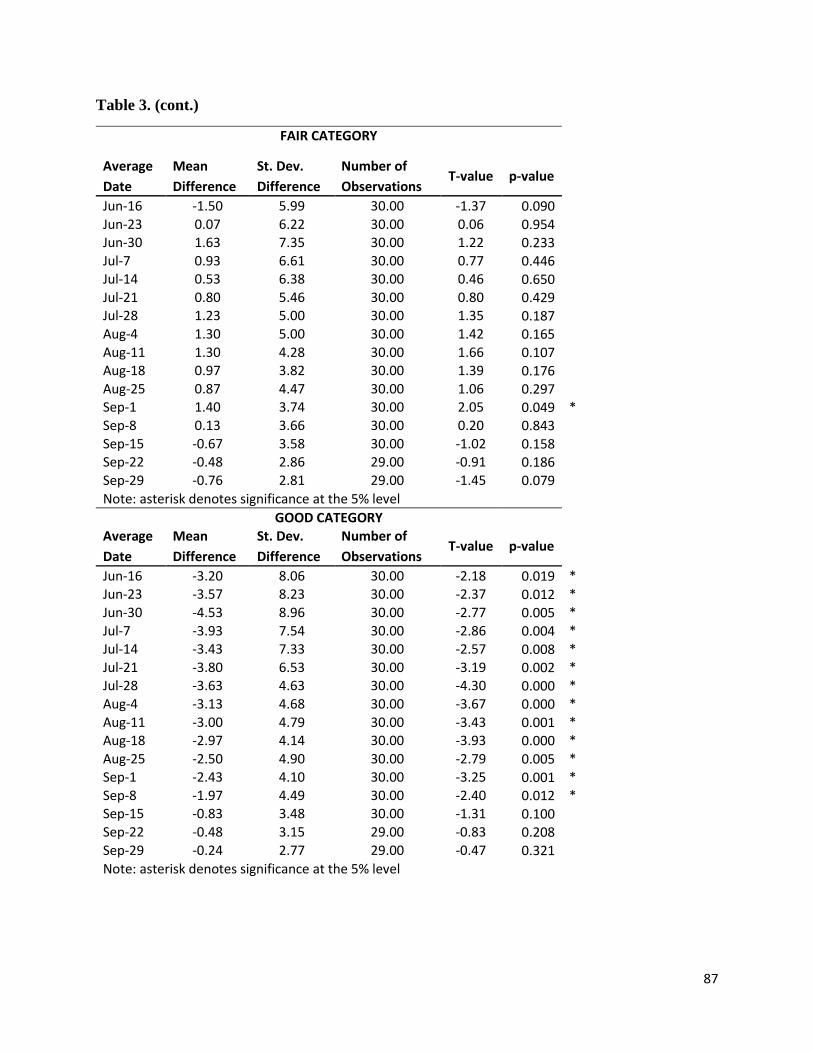
87

Table 3. (cont.)

FAIR CATEGORY

Average Mean St. Dev. Number of T-value p-value

Date Difference Difference Observations Jun-16 -1.50 5.99 30.00 -1.37 0.090 Jun-23 0.07 6.22 30.00 0.06 0.954 Jun-30 1.63 7.35 30.00 1.22 0.233 Jul-7 0.93 6.61 30.00 0.77 0.446 Jul-14 0.53 6.38 30.00 0.46 0.650 Jul-21 0.80 5.46 30.00 0.80 0.429 Jul-28 1.23 5.00 30.00 1.35 0.187 Aug-4 1.30 5.00 30.00 1.42 0.165 Aug-11 1.30 4.28 30.00 1.66 0.107 Aug-18 0.97 3.82 30.00 1.39 0.176 Aug-25 0.87 4.47 30.00 1.06 0.297 Sep-1 1.40 3.74 30.00 2.05 0.049 * Sep-8 0.13 3.66 30.00 0.20 0.843 Sep-15 -0.67 3.58 30.00 -1.02 0.158 Sep-22 -0.48 2.86 29.00 -0.91 0.186 Sep-29 -0.76 2.81 29.00 -1.45 0.079 Note: asterisk denotes significance at the 5% level

GOOD CATEGORY Average Mean St. Dev. Number of

T-value p-value Date Difference Difference Observations Jun-16 -3.20 8.06 30.00 -2.18 0.019 * Jun-23 -3.57 8.23 30.00 -2.37 0.012 * Jun-30 -4.53 8.96 30.00 -2.77 0.005 * Jul-7 -3.93 7.54 30.00 -2.86 0.004 * Jul-14 -3.43 7.33 30.00 -2.57 0.008 * Jul-21 -3.80 6.53 30.00 -3.19 0.002 * Jul-28 -3.63 4.63 30.00 -4.30 0.000 * Aug-4 -3.13 4.68 30.00 -3.67 0.000 * Aug-11 -3.00 4.79 30.00 -3.43 0.001 * Aug-18 -2.97 4.14 30.00 -3.93 0.000 * Aug-25 -2.50 4.90 30.00 -2.79 0.005 * Sep-1 -2.43 4.10 30.00 -3.25 0.001 * Sep-8 -1.97 4.49 30.00 -2.40 0.012 * Sep-15 -0.83 3.48 30.00 -1.31 0.100 Sep-22 -0.48 3.15 29.00 -0.83 0.208 Sep-29 -0.24 2.77 29.00 -0.47 0.321 Note: asterisk denotes significance at the 5% level

88

Table 3. (cont.)

EXCELLENT CATEGORY

Average Mean St. Dev. Number of T-value p-value

Date Difference Difference Observations Jun-16 1.67 3.96 30.00 2.31 0.028 *

Jun-23 0.90 4.00 30.00 1.23 0.228 Jun-30 0.23 4.30 30.00 0.30 0.769 Jul-7 -0.23 4.31 30.00 -0.30 0.385 Jul-14 -0.67 3.96 30.00 -0.92 0.182 Jul-21 -0.83 3.62 30.00 -1.26 0.109 Jul-28 -0.87 3.51 30.00 -1.35 0.093 Aug-4 -1.07 3.15 30.00 -1.85 0.037 *

Aug-11 -0.93 3.18 30.00 -1.61 0.060 Aug-18 -0.57 2.79 30.00 -1.11 0.137 Aug-25 -0.17 2.29 30.00 -0.40 0.347 Sep-1 0.03 2.09 30.00 0.09 0.931 Sep-8 0.47 2.10 30.00 1.22 0.233 Sep-15 0.63 1.90 30.00 1.82 0.079 Sep-22 0.69 1.77 29.00 2.09 0.046 *

Sep-29 0.66 1.78 29.00 1.98 0.057 Note: asterisk denotes significance at the 5% level

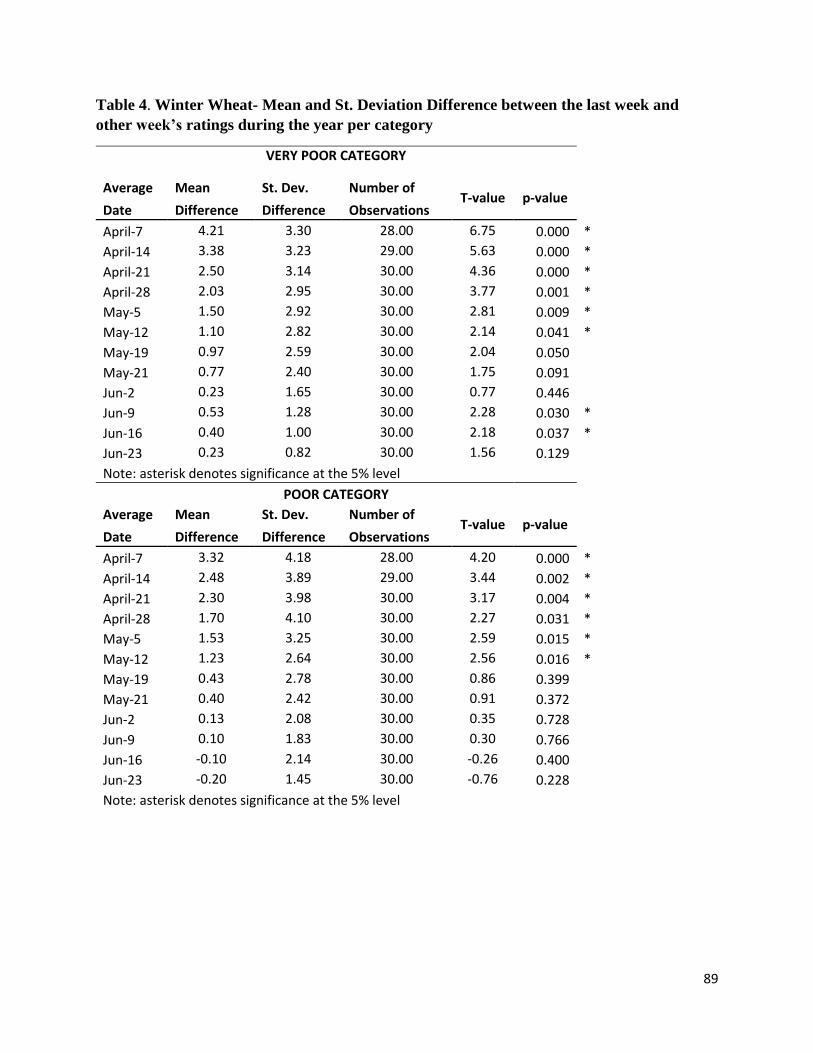
89

Table 4. Winter Wheat- Mean and St. Deviation Difference between the last week and

other week’s ratings during the year per category

VERY POOR CATEGORY

Average Mean St. Dev. Number of T-value p-value

Date Difference Difference Observations April-7 4.21 3.30 28.00 6.75 0.000 *

April-14 3.38 3.23 29.00 5.63 0.000 *

April-21 2.50 3.14 30.00 4.36 0.000 *

April-28 2.03 2.95 30.00 3.77 0.001 *

May-5 1.50 2.92 30.00 2.81 0.009 *

May-12 1.10 2.82 30.00 2.14 0.041 *

May-19 0.97 2.59 30.00 2.04 0.050 May-21 0.77 2.40 30.00 1.75 0.091 Jun-2 0.23 1.65 30.00 0.77 0.446 Jun-9 0.53 1.28 30.00 2.28 0.030 *

Jun-16 0.40 1.00 30.00 2.18 0.037 *

Jun-23 0.23 0.82 30.00 1.56 0.129 Note: asterisk denotes significance at the 5% level

POOR CATEGORY Average Mean St. Dev. Number of

T-value p-value

Date Difference Difference Observations April-7 3.32 4.18 28.00 4.20 0.000 *

April-14 2.48 3.89 29.00 3.44 0.002 *

April-21 2.30 3.98 30.00 3.17 0.004 *

April-28 1.70 4.10 30.00 2.27 0.031 *

May-5 1.53 3.25 30.00 2.59 0.015 *

May-12 1.23 2.64 30.00 2.56 0.016 *

May-19 0.43 2.78 30.00 0.86 0.399 May-21 0.40 2.42 30.00 0.91 0.372 Jun-2 0.13 2.08 30.00 0.35 0.728 Jun-9 0.10 1.83 30.00 0.30 0.766 Jun-16 -0.10 2.14 30.00 -0.26 0.400 Jun-23 -0.20 1.45 30.00 -0.76 0.228 Note: asterisk denotes significance at the 5% level

90

Table 4. (cont.)

FAIR CATEGORY Average Mean St. Dev. Number of

T-value p-value Date Difference Difference Observations April-7 -0.61 5.47 28.00 -0.59 0.281 April-14 0.41 5.03 29.00 0.44 0.661 April-21 0.03 5.14 30.00 0.04 0.972 April-28 1.07 4.54 30.00 1.29 0.208 May-5 0.83 4.05 30.00 1.13 0.269 May-12 0.37 3.34 30.00 0.60 0.552 May-19 -0.03 2.94 30.00 -0.06 0.475 May-21 -0.33 3.14 30.00 -0.58 0.283 Jun-2 -0.07 2.35 30.00 -0.16 0.439 Jun-9 -0.50 2.11 30.00 -1.30 0.103 Jun-16 -0.43 2.49 30.00 -0.95 0.174 Jun-23 -0.37 1.52 30.00 -1.32 0.098 Note: asterisk denotes significance at the 5% level

GOOD CATEGORY Average Mean St. Dev. Number of

T-value p-value Date Difference Difference Observations April-7 -6.36 5.59 28.00 -6.02 0.000 *

April-14 -6.03 4.57 29.00 -7.11 0.000 *

April-21 -4.93 5.58 30.00 -4.85 0.000 *

April-28 -4.57 5.60 30.00 -4.47 0.000 *

May-5 -3.83 5.11 30.00 -4.11 0.000 *

May-12 -2.77 4.14 30.00 -3.66 0.001 *

May-19 -1.77 4.39 30.00 -2.20 0.018 *

May-21 -1.30 3.93 30.00 -1.81 0.040 *

Jun-2 -0.67 3.42 30.00 -1.07 0.147 Jun-9 -0.53 2.80 30.00 -1.04 0.153 Jun-16 -0.33 2.45 30.00 -0.74 0.231 Jun-23 0.07 1.57 30.00 0.23 0.818 Note: asterisk denotes significance at the 5% level

91

Table 4. (cont.)

EXCELLENT CATEGORY Average Mean St. Dev. Number of

T-value p-value

Date Difference Difference Observations April-7 -0.57 3.51 28.00 -0.86 0.198 April-14 -0.24 3.46 29.00 -0.38 0.355 April-21 0.10 3.54 30.00 0.15 0.878 April-28 -0.23 3.29 30.00 -0.39 0.350 May-5 -0.03 3.27 30.00 -0.06 0.478 May-12 0.07 3.06 30.00 0.12 0.906 May-19 0.40 2.62 30.00 0.84 0.410 May-21 0.47 2.50 30.00 1.02 0.315 Jun-2 0.37 2.22 30.00 0.90 0.373 Jun-9 0.40 1.67 30.00 1.31 0.201 Jun-16 0.47 1.57 30.00 1.63 0.114 Jun-23 0.27 0.98 30.00 1.49 0.147 Note: asterisk denotes significance at the 5% level

92

Table 5. Spring Wheat- Mean and St. Deviation Difference between the last week and other

week’s ratings during the year per category

VERY POOR CATEGORY

Average Mean St. Dev. Number of T-value p-value

Date Difference Difference Observations Jun-9 3.00 3.77 30.00 4.36 0.000 *

Jun-16 2.73 3.30 30.00 4.54 0.000 *

Jun-23 2.27 2.63 30.00 4.73 0.000 *

Jun-30 1.83 2.31 30.00 4.36 0.000 *

Jul-7 1.30 1.80 30.00 3.95 0.000 *

Jul-14 1.10 1.32 30.00 4.56 0.000 *

Jul-21 0.93 1.66 30.00 3.08 0.004 *

Jul-28 0.53 1.46 30.00 2.01 0.054 Aug-4 0.52 1.12 29.00 2.48 0.019 *

Note: asterisk denotes significance at the 5% level

POOR CATEGORY Average Mean St. Dev. Number of

T-value p-value Date Difference Difference Observations Jun-9 5.10 4.96 30.00 5.63 0.000 *

Jun-16 4.47 5.22 30.00 4.69 0.000 *

Jun-23 4.03 4.82 30.00 4.59 0.000 *

Jun-30 3.60 4.34 30.00 4.55 0.000 *

Jul-7 2.67 4.37 30.00 3.35 0.002 *

Jul-14 2.60 3.64 30.00 3.92 0.001 *

Jul-21 2.43 3.76 30.00 3.55 0.001 *

Jul-28 1.70 3.37 30.00 2.76 0.010 *

Aug-4 1.41 3.26 29.00 2.34 0.027 *

Note: asterisk denotes significance at the 5% level

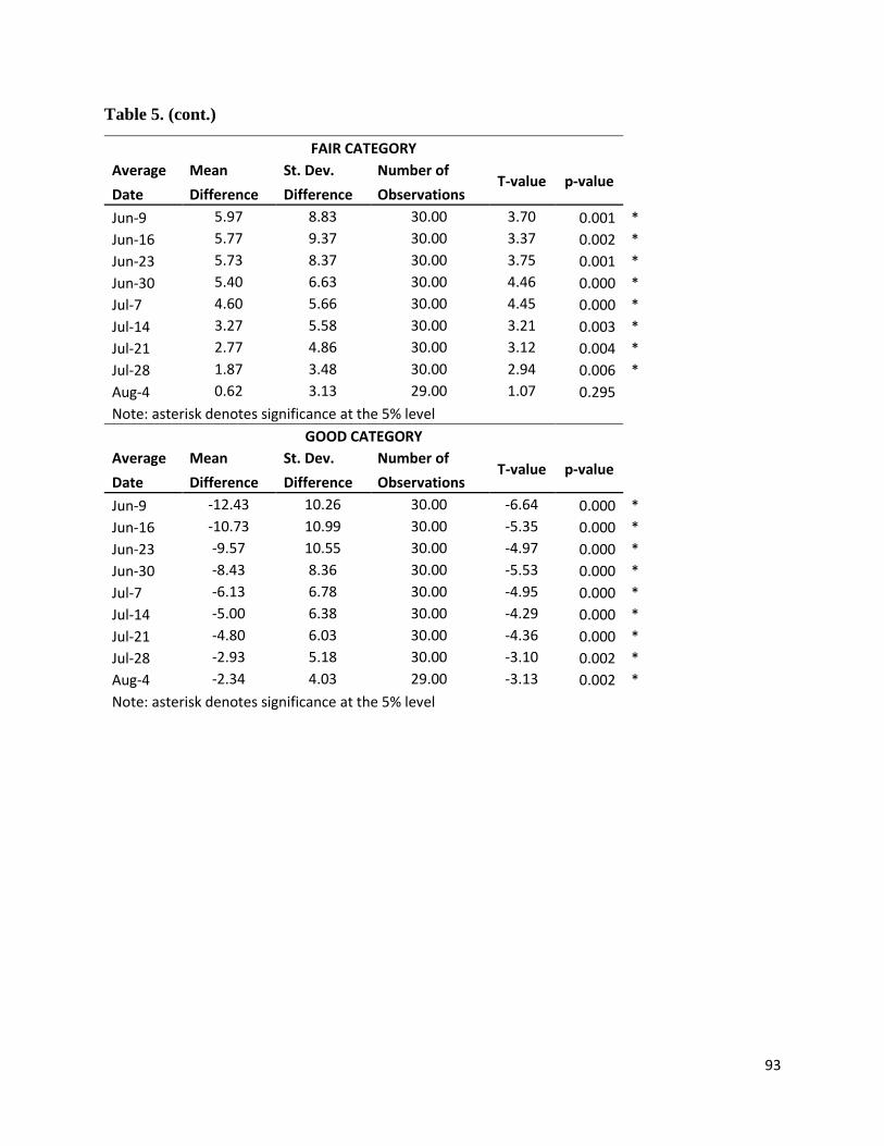
93

Table 5. (cont.)

FAIR CATEGORY Average Mean St. Dev. Number of

T-value p-value Date Difference Difference Observations Jun-9 5.97 8.83 30.00 3.70 0.001 *

Jun-16 5.77 9.37 30.00 3.37 0.002 *

Jun-23 5.73 8.37 30.00 3.75 0.001 *

Jun-30 5.40 6.63 30.00 4.46 0.000 *

Jul-7 4.60 5.66 30.00 4.45 0.000 *

Jul-14 3.27 5.58 30.00 3.21 0.003 *

Jul-21 2.77 4.86 30.00 3.12 0.004 *

Jul-28 1.87 3.48 30.00 2.94 0.006 *

Aug-4 0.62 3.13 29.00 1.07 0.295 Note: asterisk denotes significance at the 5% level

GOOD CATEGORY Average Mean St. Dev. Number of

T-value p-value Date Difference Difference Observations Jun-9 -12.43 10.26 30.00 -6.64 0.000 *

Jun-16 -10.73 10.99 30.00 -5.35 0.000 *

Jun-23 -9.57 10.55 30.00 -4.97 0.000 *

Jun-30 -8.43 8.36 30.00 -5.53 0.000 *

Jul-7 -6.13 6.78 30.00 -4.95 0.000 *

Jul-14 -5.00 6.38 30.00 -4.29 0.000 *

Jul-21 -4.80 6.03 30.00 -4.36 0.000 *

Jul-28 -2.93 5.18 30.00 -3.10 0.002 *

Aug-4 -2.34 4.03 29.00 -3.13 0.002 *

Note: asterisk denotes significance at the 5% level

94

Table 5. (cont.)

EXCELLENT CATEGORY Average Mean St. Dev. Number of

T-value p-value Date Difference Difference Observations Jun-9 -1.63 4.99 30.00 -1.79 0.042 *

Jun-16 -2.23 5.98 30.00 -2.05 0.025 *

Jun-23 -2.47 4.90 30.00 -2.76 0.005 *

Jun-30 -2.40 4.52 30.00 -2.91 0.003 *

Jul-7 -2.43 4.34 30.00 -3.07 0.002 *

Jul-14 -1.97 3.71 30.00 -2.90 0.003 *

Jul-21 -1.33 2.94 30.00 -2.48 0.010 *

Jul-28 -1.17 2.76 30.00 -2.32 0.014 *

Aug-4 -0.21 2.40 29.00 -0.46 0.323 Note: asterisk denotes significance at the 5% level

95

Figure 6. Corn- Mean Difference of Ratings for Each Category per Week for Years 1986 to

2015, June 2-39

-10.00

-8.00

-6.00

-4.00

-2.00

0.00

2.00

4.00

6.00

Jun

-2

Jun

-9

Jun

-16

Jun

-23

Jun

-30

Jul-

7

Jul-

14

Jul-

21

Jul-

28

Au

g-4

Au

g-1

1

Au

g-1

8

Au

g-2

5

Sep

-1

Sep

-8

Sep

-15

Sep

-22

Sep

-29

Mea

n D

iffe

ren

ce

Corn-Mean Difference Very Poor Category by Week for Years 1986-2015

MEAN

-10.00

-8.00

-6.00

-4.00

-2.00

0.00

2.00

4.00

6.00

Jun

-2

Jun

-9

Jun

-16

Jun

-23

Jun

-30

Jul-

7

Jul-

14

Jul-

21

Jul-

28

Au

g-4

Au

g-1

1

Au

g-1

8

Au

g-2

5

Sep

-1

Sep

-8

Sep

-15

Sep

-22

Sep

-29

Mea

n D

iffe

ren

ce

Corn-Mean Difference Poor Category by Week for Years 1986-2015

MEAN

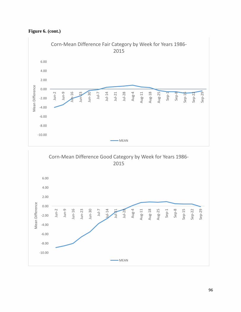
96

Figure 6. (cont.)

-10.00

-8.00

-6.00

-4.00

-2.00

0.00

2.00

4.00

6.00

Jun

-2

Jun

-9

Jun

-16

Jun

-23

Jun

-30

Jul-

7

Jul-

14

Jul-

21

Jul-

28

Au

g-4

Au

g-1

1

Au

g-1

8

Au

g-2

5

Sep

-1

Sep

-8

Sep

-15

Sep

-22

Sep

-29

Mea

n D

iffe

ren

ce

Corn-Mean Difference Fair Category by Week for Years 1986-2015

MEAN

-10.00

-8.00

-6.00

-4.00

-2.00

0.00

2.00

4.00

6.00

Jun

-2

Jun

-9

Jun

-16

Jun

-23

Jun

-30

Jul-

7

Jul-

14

Jul-

21

Jul-

28

Au

g-4

Au

g-1

1

Au

g-1

8

Au

g-2

5

Sep

-1

Sep

-8

Sep

-15

Sep

-22

Sep

-29

Mea

n D

iffe

ren

ce

Corn-Mean Difference Good Category by Week for Years 1986-2015

MEAN

97

Figure 6. (cont.)

-10.00

-8.00

-6.00

-4.00

-2.00

0.00

2.00

4.00

6.00

Jun

-2

Jun

-9

Jun

-16

Jun

-23

Jun

-30

Jul-

7

Jul-

14

Jul-

21

Jul-

28

Au

g-4

Au

g-1

1

Au

g-1

8

Au

g-2

5

Sep

-1

Sep

-8

Sep

-15

Sep

-22

Sep

-29

Mea

n D

iffe

ren

ce

Corn-Mean Difference Excellent Category by Week for Years 1986-2015

MEAN

98

Figure 7. Soybeans- Mean Difference of Ratings for Each Category per Week for Years

1986 to 2015, June 16-39

-10.00

-8.00

-6.00

-4.00

-2.00

0.00

2.00

4.00

Jun

-16

Jun

-23

Jun

-30

Jul-

7

Jul-

14

Jul-

21

Jul-

28

Au

g-4

Au

g-1

1

Au

g-1

8

Au

g-2

5

Sep

-1

Sep

-8

Sep

-15

Sep

-22

Sep

-29

Mea

n D

iffe

ren

ce

Soybeans- Mean Difference Very Poor Category by Week for Years 1986- 2015

MEAN

-10.00

-8.00

-6.00

-4.00

-2.00

0.00

2.00

4.00

Jun

-16

Jun

-23

Jun

-30

Jul-

7

Jul-

14

Jul-

21

Jul-

28

Au

g-4

Au

g-1

1

Au

g-1

8

Au

g-2

5

Sep

-1

Sep

-8

Sep

-15

Sep

-22

Sep

-29

Mea

n D

iffe

ren

ce

Soybeans- Mean Difference Poor Category by Week for Years 1986- 2015

MEAN

99

Figure 7. (cont.)

-10.00

-8.00

-6.00

-4.00

-2.00

0.00

2.00

4.00

Jun

-16

Jun

-23

Jun

-30

Jul-

7

Jul-

14

Jul-

21

Jul-

28

Au

g-4

Au

g-1

1

Au

g-1

8

Au

g-2

5

Sep

-1

Sep

-8

Sep

-15

Sep

-22

Sep

-29

Mea

n D

iffe

ren

ce

Soybeans- Mean Difference Fair Category by Week for Years 1986- 2015

MEAN

-10.00

-8.00

-6.00

-4.00

-2.00

0.00

2.00

4.00

Jun

-16

Jun

-23

Jun

-30

Jul-

7

Jul-

14

Jul-

21

Jul-

28

Au

g-4

Au

g-1

1

Au

g-1

8

Au

g-2

5

Sep

-1

Sep

-8

Sep

-15

Sep

-22

Sep

-29

Mea

n D

iffe

ren

ce

Soybeans- Mean Difference Good Category by Week for Years 1986- 2015

MEAN

100

Figure 7. (cont.)

-10.00

-8.00

-6.00

-4.00

-2.00

0.00

2.00

4.00

Jun

-16

Jun

-23

Jun

-30

Jul-

7

Jul-

14

Jul-

21

Jul-

28

Au

g-4

Au

g-1

1

Au

g-1

8

Au

g-2

5

Sep

-1

Sep

-8

Sep

-15

Sep

-22

Sep

-29

Mea

n D

iffe

ren

ce

Soybeans- Mean Difference Excellent Category by Week for Years 1986- 2015

MEAN

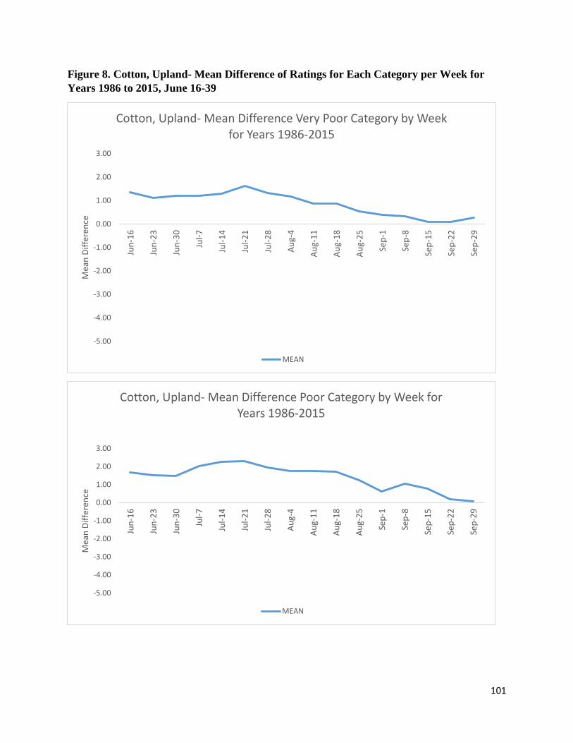
101

Figure 8. Cotton, Upland- Mean Difference of Ratings for Each Category per Week for

Years 1986 to 2015, June 16-39

-5.00

-4.00

-3.00

-2.00

-1.00

0.00

1.00

2.00

3.00

Jun

-16

Jun

-23

Jun

-30

Jul-

7

Jul-

14

Jul-

21

Jul-

28

Au

g-4

Au

g-1

1

Au

g-1

8

Au

g-2

5

Sep

-1

Sep

-8

Sep

-15

Sep

-22

Sep

-29

Mea

n D

iffe

ren

ce

Cotton, Upland- Mean Difference Very Poor Category by Week for Years 1986-2015

MEAN

-5.00

-4.00

-3.00

-2.00

-1.00

0.00

1.00

2.00

3.00

Jun

-16

Jun

-23

Jun

-30

Jul-

7

Jul-

14

Jul-

21

Jul-

28

Au

g-4

Au

g-1

1

Au

g-1

8

Au

g-2

5

Sep

-1

Sep

-8

Sep

-15

Sep

-22

Sep

-29

Mea

n D

iffe

ren

ce

Cotton, Upland- Mean Difference Poor Category by Week for Years 1986-2015

MEAN

102

Figure 8. (cont.)

-5.00

-4.00

-3.00

-2.00

-1.00

0.00

1.00

2.00

3.00

Jun

-16

Jun

-23

Jun

-30

Jul-

7

Jul-

14

Jul-

21

Jul-

28

Au

g-4

Au

g-1

1

Au

g-1

8

Au

g-2

5

Sep

-1

Sep

-8

Sep

-15

Sep

-22

Sep

-29

Mea

n D

iffe

ren

ce

Cotton, Upland- Mean Difference Fair Category by Week for Years 1986-2015

MEAN

-5.00

-4.00

-3.00

-2.00

-1.00

0.00

1.00

2.00

3.00

Jun

-16

Jun

-23

Jun

-30

Jul-

7

Jul-

14

Jul-

21

Jul-

28

Au

g-4

Au

g-1

1

Au

g-1

8

Au

g-2

5

Sep

-1

Sep

-8

Sep

-15

Sep

-22

Sep

-29

Mea

n D

iffe

ren

ce

Cotton, Upland- Mean Difference Good Category by Week for Years 1986-2015

MEAN

103

Figure 8. (cont.)

-5.00

-4.00

-3.00

-2.00

-1.00

0.00

1.00

2.00

3.00

Jun

-16

Jun

-23

Jun

-30

Jul-

7

Jul-

14

Jul-

21

Jul-

28

Au

g-4

Au

g-1

1

Au

g-1

8

Au

g-2

5

Sep

-1

Sep

-8

Sep

-15

Sep

-22

Sep

-29

Mea

n D

iffe

ren

ce

Cotton, Upland- Mean Difference Excellent Category by Week for Years 1986-2015

MEAN

104

Figure 9. Winter Wheat- Mean Difference of Ratings for Each Category per Week for

Years 1986 to 2015, April 7-25

-7.00

-5.00

-3.00

-1.00

1.00

3.00

5.00

Ap

ril-

7

Ap

ril-

14

Ap

ril-

21

Ap

ril-

28

May

-5

May

-12

May

-19

May

-21

Jun

-2

Jun

-9

Jun

-16

Jun

-23

Mea

n D

iffe

ren

ce

Winter Wheat - Mean Difference Very Poor Category by Week for Years 1986- 2015

MEAN

-7.00

-5.00

-3.00

-1.00

1.00

3.00

5.00

Ap

ril-

7

Ap

ril-

14

Ap

ril-

21

Ap

ril-

28

May

-5

May

-12

May

-19

May

-21

Jun

-2

Jun

-9

Jun

-16

Jun

-23

Mea

n D

iffe

ren

ce

Winter Wheat - Mean Difference Poor Category by Week for Years 1986- 2015

MEAN

105

Figure 9. (cont.)

-7.00

-5.00

-3.00

-1.00

1.00

3.00

5.00

Ap

ril-

7

Ap

ril-

14

Ap

ril-

21

Ap

ril-

28

May

-5

May

-12

May

-19

May

-21

Jun

-2

Jun

-9

Jun

-16

Jun

-23

Mea

n D

iffe

ren

ce

Winter Wheat - Mean Difference Fair Category by Week for Years 1986- 2015

MEAN

-7.00

-5.00

-3.00

-1.00

1.00

3.00

5.00

Ap

ril-

7

Ap

ril-

14

Ap

ril-

21

Ap

ril-

28

May

-5

May

-12

May

-19

May

-21

Jun

-2

Jun

-9

Jun

-16

Jun

-23

Mea

n D

iffe

ren

ce

Winter Wheat - Mean Difference Good Category by Week for Years 1986- 2015

MEAN

106

Figure 9. (cont.)

-7.00

-5.00

-3.00

-1.00

1.00

3.00

5.00

Ap

ril-

7

Ap

ril-

14

Ap

ril-

21

Ap

ril-

28

May

-5

May

-12

May

-19

May

-21

Jun

-2

Jun

-9

Jun

-16

Jun

-23

Mea

n D

iffe

ren

ce

Winter Wheat - Mean Difference Excellent Category by Week for Years 1986- 2015

MEAN

107

Figure 10. Spring Wheat- Mean Difference of Ratings for Each Category per Week for

Years 1986 to 2015, June 9-31

-14.00

-9.00

-4.00

1.00

6.00

Jun

-9

Jun

-16

Jun

-23

Jun

-30

Jul-

7

Jul-

14

Jul-

21

Jul-

28

Au

g-4

Mea

n D

iffe

ren

ce

Spring Wheat-Mean Difference Very Poor Category by Week for Years 1986-2015

MEAN

-14.00

-9.00

-4.00

1.00

6.00

Jun

-9

Jun

-16

Jun

-23

Jun

-30

Jul-

7

Jul-

14

Jul-

21

Jul-

28

Au

g-4

Mea

n D

iffe

ren

ce

Spring Wheat-Mean Difference Poor Category by Week for Years 1986-2015

MEAN

108

Figure 10. (cont.)

-14.00

-9.00

-4.00

1.00

6.00

Jun

-9

Jun

-16

Jun

-23

Jun

-30

Jul-

7

Jul-

14

Jul-

21

Jul-

28

Au

g-4

Mea

n D

iffe

ren

ce

Spring Wheat-Mean Difference Fair Category by Week for Years 1986-2015

MEAN

-14.00

-12.00

-10.00

-8.00

-6.00

-4.00

-2.00

0.00

2.00

4.00

6.00

Jun

-9

Jun

-16

Jun

-23

Jun

-30

Jul-

7

Jul-

14

Jul-

21

Jul-

28

Au

g-4

Mea

n D

iffe

ren

ce

Spring Wheat-Mean Difference Good Category by Week for Years 1986-2015

MEAN

109

Figure 10. (cont.)

-14.00

-9.00

-4.00

1.00

6.00

Jun

-9

Jun

-16

Jun

-23

Jun

-30

Jul-

7

Jul-

14

Jul-

21

Jul-

28

Au

g-4

Mea

n D

iffe

ren

ce

Spring Wheat-Mean Difference Excellent Category by Week for Years 1986-2015

MEAN

110

Figure 11. Corn- Standard Deviation of Ratings per Week, 1986-2015

0

2

4

6

8

10

12

Jun

-2

Jun

-9

Jun

-16

Jun

-23

Jun

-30

Jul-

7

Jul-

14

Jul-

21

Jun

-28

Au

g-4

Au

g-1

1

Au

g-1

8

Au

g-2

5

Sep

-1

Sep

-8

Sep

-15

Sep

-22

Sep

-29

St.D

evia

tio

n

Corn-St.Deviation Very Poor Category by Week for Years 1986-2015

St.Deviation

0

2

4

6

8

10

12

Jun

-2

Jun

-9

Jun

-16

Jun

-23

Jun

-30

Jul-

7

Jul-

14

Jul-

21

Jun

-28

Au

g-4

Au

g-1

1

Au

g-1

8

Au

g-2

5

Sep

-1

Sep

-8

Sep

-15

Sep

-22

Sep

-29

St.D

evia

tio

n

Corn-St.Deviation Poor Category by Week for Years 1986-2015

St.Deviation

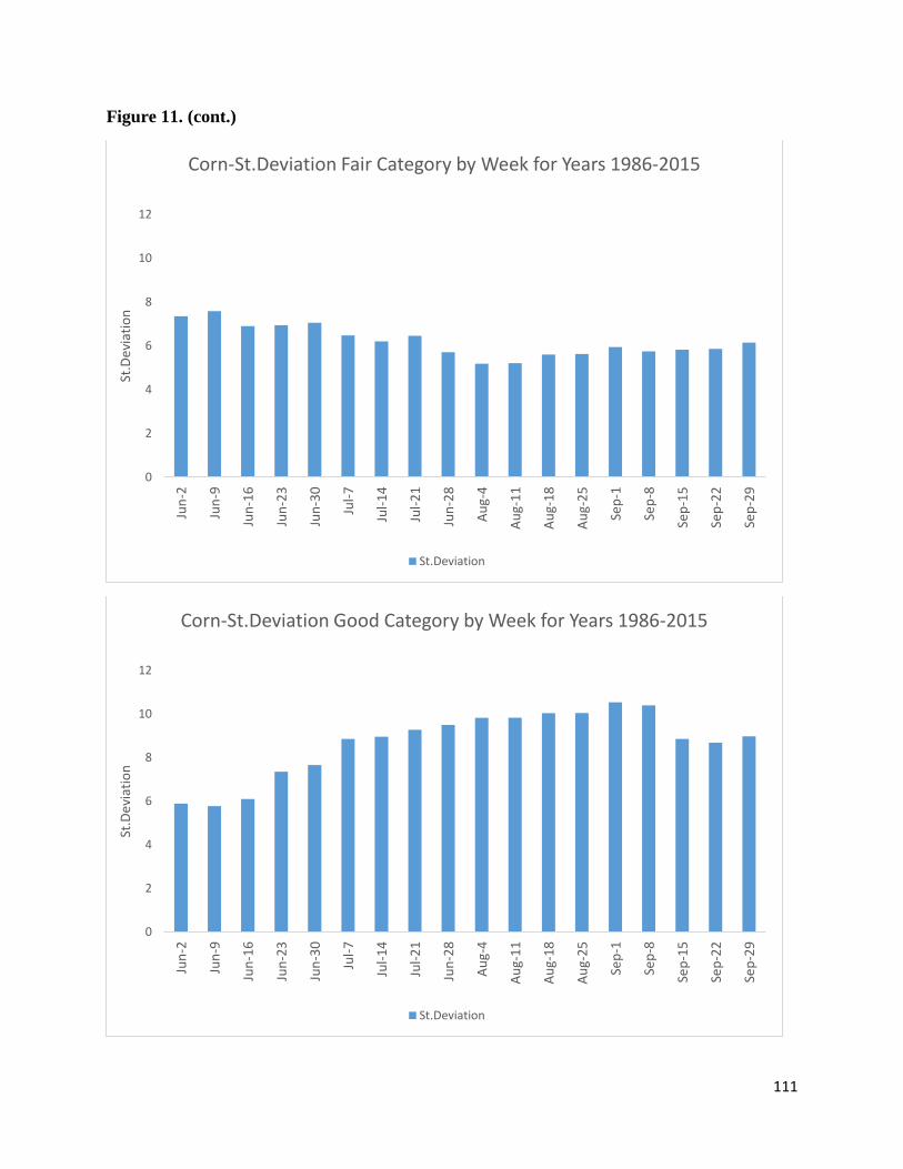
111

Figure 11. (cont.)

0

2

4

6

8

10

12

Jun

-2

Jun

-9

Jun

-16

Jun

-23

Jun

-30

Jul-

7

Jul-

14

Jul-

21

Jun

-28

Au

g-4

Au

g-1

1

Au

g-1

8

Au

g-2

5

Sep

-1

Sep

-8

Sep

-15

Sep

-22

Sep

-29

St.D

evia

tio

n

Corn-St.Deviation Fair Category by Week for Years 1986-2015

St.Deviation

0

2

4

6

8

10

12

Jun

-2

Jun

-9

Jun

-16

Jun

-23

Jun

-30

Jul-

7

Jul-

14

Jul-

21

Jun

-28

Au

g-4

Au

g-1

1

Au

g-1

8

Au

g-2

5

Sep

-1

Sep

-8

Sep

-15

Sep

-22

Sep

-29

St.D

evia

tio

n

Corn-St.Deviation Good Category by Week for Years 1986-2015

St.Deviation

112

Figure 11. (cont.)

0

2

4

6

8

10

12

Jun

-2

Jun

-9

Jun

-16

Jun

-23

Jun

-30

Jul-

7

Jul-

14

Jul-

21

Jun

-28

Au

g-4

Au

g-1

1

Au

g-1

8

Au

g-2

5

Sep

-1

Sep

-8

Sep

-15

Sep

-22

Sep

-29

St.D

evia

tio

n

Corn-St.Deviation Excellent Category by Week for Years 1986-2015

St.Deviation

113

Figure 12. Soybeans- Standard Deviation of Ratings per Week, 1986-2015

0

1

2

3

4

5

6

7

8

9

10

Jun

-16

Jun

-23

Jun

-30

Jul-

7

Jul-

14

Jul-

21

Jun

-28

Au

g-4

Au

g-1

1

Au

g-1

8

Jun

-25

Sep

-1

Sep

-8

Sep

-15

Sep

-22

Sep

-29

St.D

evia

tio

n

Soybeans-St.Deviation Very Poor Category by Week for Years 1986-2015

St.Deviation

0

1

2

3

4

5

6

7

8

9

10

Jun

-16

Jun

-23

Jun

-30

Jul-

7

Jul-

14

Jul-

21

Jun

-28

Au

g-4

Au

g-1

1

Au

g-1

8

Jun

-25

Sep

-1

Sep

-8

Sep

-15

Sep

-22

Sep

-29

St.D

evia

tio

n

Soybeans-St.Deviation Poor Category by Week for Years 1986-2015

St.Deviation

114

Figure 12. (cont.)

0

1

2

3

4

5

6

7

8

9

10

Jun

-16

Jun

-23

Jun

-30

Jul-

7

Jul-

14

Jul-

21

Jun

-28

Au

g-4

Au

g-1

1

Au

g-1

8

Jun

-25

Sep

-1

Sep

-8

Sep

-15

Sep

-22

Sep

-29

St.D

evia

tio

n

Soybeans-St.Deviation Fair Category by Week for Years 1986-2015

St.Deviation

0

1

2

3

4

5

6

7

8

9

10

Jun

-16

Jun

-23

Jun

-30

Jul-

7

Jul-

14

Jul-

21

Jun

-28

Au

g-4

Au

g-1

1

Au

g-1

8

Jun

-25

Sep

-1

Sep

-8

Sep

-15

Sep

-22

Sep

-29

St.D

evia

tio

n

Soybeans-St.Deviation Good Category by Week for Years 1986-2015

St.Deviation

115

Figure 12. (cont.)

0

1

2

3

4

5

6

7

8

9

10

Jun

-16

Jun

-23

Jun

-30

Jul-

7

Jul-

14

Jul-

21

Jun

-28

Au

g-4

Au

g-1

1

Au

g-1

8

Jun

-25

Sep

-1

Sep

-8

Sep

-15

Sep

-22

Sep

-29

St.D

evia

tio

n

Soybeans-St.Deviation Excellent Category by Week for Years 1986-2015

St.Deviation

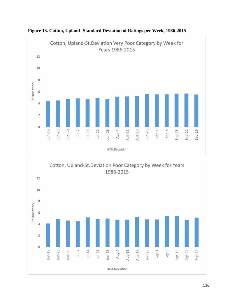
116

Figure 13. Cotton, Upland- Standard Deviation of Ratings per Week, 1986-2015

0

2

4

6

8

10

12

Jun

-16

Jun

-23

Jun

-30

Jul-

7

Jul-

14

Jul-

21

Jun

-28

Au

g-4

Au

g-1

1

Au

g-1

8

Jun

-25

Sep

-1

Sep

-8

Sep

-15

Sep

-22

Sep

-29

St.D

evia

tio

n

Cotton, Upland-St.Deviation Very Poor Category by Week for Years 1986-2015

St.Deviation

0

2

4

6

8

10

12

Jun

-16

Jun

-23

Jun

-30

Jul-

7

Jul-

14

Jul-

21

Jun

-28

Au

g-4

Au

g-1

1

Au

g-1

8

Jun

-25

Sep

-1

Sep

-8

Sep

-15

Sep

-22

Sep

-29

St.D

evia

tio

n

Cotton, Upland-St.Deviation Poor Category by Week for Years 1986-2015

St.Deviation

117

Figure 13. (cont.)

0

2

4

6

8

10

12

Jun

-16

Jun

-23

Jun

-30

Jul-

7

Jul-

14

Jul-

21

Jun

-28

Au

g-4

Au

g-1

1

Au

g-1

8

Jun

-25

Sep

-1

Sep

-8

Sep

-15

Sep

-22

Sep

-29

St.D

evia

tio

n

Cotton, Upland-St.Deviation Fair Category by Week for Years 1986-2015

St.Deviation

0

2

4

6

8

10

12

Jun

-16

Jun

-23

Jun

-30

Jul-

7

Jul-

14

Jul-

21

Jun

-28

Au

g-4

Au

g-1

1

Au

g-1

8

Jun

-25

Sep

-1

Sep

-8

Sep

-15

Sep

-22

Sep

-29

St.D

evia

tio

n

Cotton, Upland-St.Deviation Good Category by Week for Years 1986-2015

St.Deviation

118

Figure 13. (cont.)

0

2

4

6

8

10

12

Jun

-16

Jun

-23

Jun

-30

Jul-

7

Jul-

14

Jul-

21

Jun

-28

Au

g-4

Au

g-1

1

Au

g-1

8

Jun

-25

Sep

-1

Sep

-8

Sep

-15

Sep

-22

Sep

-29

St.D

evia

tio

n

Cotton, Upland-St.Deviation Excellent Category by Week for Years 1986-2015

St.Deviation

119

Figure 14. Winter Wheat- Standard Deviation of Ratings per Week, 1986-2015

0

2

4

6

8

10

12

Ap

ril-

7

Ap

ril-

14

Ap

ril-

21

Ap

ril-

28

May

-5

May

-12

May

-19

May

-21

Jun

-2

Jun

-9

Jun

-16

Jun

-23

St.D

evia

tio

n

Winter Wheat-St.Deviation Very Poor Category by Week for Years 1986-2015

St.Deviation

0

2

4

6

8

10

12

Ap

ril-

7

Ap

ril-

14

Ap

ril-

21

Ap

ril-

28

May

-5

May

-12

May

-19

May

-21

Jun

-2

Jun

-9

Jun

-16

Jun

-23

St.D

evia

tio

n

Winter Wheat-St.Deviation Poor Category by Week for Years 1986-2015

St.Deviation

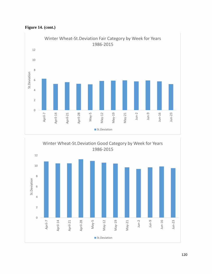
120

Figure 14. (cont.)

0

2

4

6

8

10

12

Ap

ril-

7

Ap

ril-

14

Ap

ril-

21

Ap

ril-

28

May

-5

May

-12

May

-19

May

-21

Jun

-2

Jun

-9

Jun

-16

Jun

-23

St.D

evia

tio

n

Winter Wheat-St.Deviation Fair Category by Week for Years 1986-2015

St.Deviation

0

2

4

6

8

10

12

Ap

ril-

7

Ap

ril-

14

Ap

ril-

21

Ap

ril-

28

May

-5

May

-12

May

-19

May

-21

Jun

-2

Jun

-9

Jun

-16

Jun

-23

St.D

evia

tio

n

Winter Wheat-St.Deviation Good Category by Week for Years 1986-2015

St.Deviation

121

Figure 14. (cont.)

0

2

4

6

8

10

12

Ap

ril-

7

Ap

ril-

14

Ap

ril-

21

Ap

ril-

28

May

-5

May

-12

May

-19

May

-21

Jun

-2

Jun

-9

Jun

-16

Jun

-23

St.D

evia

tio

n

Winter Wheat-St.Deviation Excellent Category by Week for Years 1986-2015

St.Deviation

122

Figure 15. Spring Wheat- Standard Deviation of Ratings per Week, 1986-2015

0

2

4

6

8

10

12

14

Jun

-9

Jun

-16

Jun

-23

Jun

-30

Jul-

7

Jul-

14

Jul-

21

Jul-

28

Au

g-4

St.D

evia

tio

n

Spring Wheat-St.Deviation Very Poor Category by Week for Years 1986-2015

St.Deviation

0

2

4

6

8

10

12

14

Jun

-9

Jun

-16

Jun

-23

Jun

-30

Jul-

7

Jul-

14

Jul-

21

Jul-

28

Au

g-4

St.D

evia

tio

n

Spring Wheat-St.Deviation Poor Category by Week for Years 1986-2015

St.Deviation

123

Figure 15. (cont.)

0

2

4

6

8

10

12

14

Jun

-9

Jun

-16

Jun

-23

Jun

-30

Jul-

7

Jul-

14

Jul-

21

Jul-

28

Au

g-4

St.D

evia

tio

n

Spring Wheat-St.Deviation Fair Category by Week for Years 1986-2015

St.Deviation

0

2

4

6

8

10

12

14

Jun

-9

Jun

-16

Jun

-23

Jun

-30

Jul-

7

Jul-

14

Jul-

21

Jul-

28

Au

g-4

St.D

evia

tio

n

Spring Wheat-St.Deviation Good Category by Week for Years 1986-2015

St.Deviation

124

Figure 15. (cont.)

0

2

4

6

8

10

12

14

Jun

-9

Jun

-16

Jun

-23

Jun

-30

Jul-

7

Jul-

14

Jul-

21

Jul-

28

Au

g-4

St.D

evia

tio

n

Spring Wheat-St.Deviation Excellent Category by Week for Years 1986-2015

St.Deviation

125

Figure 16. Average U.S Corn Yield, 1986-2015

CORN YIELD in BU / ACRE

Mean 135.5

Standard Error 3.7

Median 135.6

Mode N/A

Standard Deviation 20.5

Sample Variance 420.9

Kurtosis -0.04

Skewness -0.32

Range 86.4

Minimum 84.6

Maximum 171

Sum 4065.8

Count 30

Largest(1) 171

Smallest(1) 84.6

y = 1.9075x + 105.96R² = 0.6699

0.0

20.0

40.0

60.0

80.0

100.0

120.0

140.0

160.0

180.0

19

86

19

87

19

88

19

89

19

90

19

91

19

92

19

93

19

94

19

95

19

96

19

97

19

98

19

99

20

00

20

01

20

02

20

03

20

04

20

05

20

06

20

07

20

08

20

09

20

10

20

11

20

12

20

13

20

14

20

15

Yiel

d (

bu

shel

s p

er a

cre)

Year

126

Figure 17. Average U.S Soybean Yield, 1986-2015

y = 0.4659x + 31.508R² = 0.7238

0

10

20

30

40

50

60

19

86

19

87

19

88

19

89

19

90

19

91

19

92

19

93

19

94

19

95

19

96

19

97

19

98

19

99

20

00

20

01

20

02

20

03

20

04

20

05

20

06

20

07

20

08

20

09

20

10

20

11

20

12

20

13

20

14

20

15

Yiel

d (

bu

shel

s p

er a

cre)

Year

SOYBEAN YIELD in BU / ACRE

Mean 38.7

Standard Error 0.9

Median 38.9

Mode 33.9

Standard Deviation 4.8

Sample Variance 23.3

Kurtosis -0.1

Skewness -0.2

Range 21

Minimum 27

Maximum 48

Sum 1161.9

Count 30

Largest(1) 48

Smallest(1) 27

127

Figure 18. Average U.S Cotton, Upland Yield, 1986-2015

COTTON, UPLAND YIELD in LB / ACRE

Mean 718.7

Standard Error 18.3

Median 705.5

Mode 705.0

Standard Deviation 100.0

Sample Variance 10003.3

Kurtosis -1.1

Skewness 0.0

Range 355.0

Minimum 537.0

Maximum 892.0

Sum 21560.0

Count 30.0

Largest(1) 892.0

Smallest(1) 537.0

y = 8.5964x + 576.66R² = 0.6055

0

100

200

300

400

500

600

700

800

900

1000

19

86

19

87

19

88

19

89

19

90

19

91

19

92

19

93

19

94

19

95

19

96

19

97

19

98

19

99

20

00

20

01

20

02

20

03

20

04

20

05

20

06

20

07

20

08

20

09

20

10

20

11

20

12

20

13

20

14

20

15

Yiel

d (

po

un

ds

per

acr

e)

Year

128

Figure 19. Average U.S Winter Wheat Yield, 1986-2015

WINTER WHEAT YIELD in BU / ACRE

Mean 42.6

Standard Error 0.7

Median 42.6

Mode 38.2

Standard Deviation 4.0

Sample Variance 16.0

Kurtosis -0.1

Skewness -0.3

Range 13.1

Minimum 34.7

Maximum 47.8

Sum 1264.5

Count 30

Largest(1) 47.8

Smallest(1) 34.7

y = 0.3106x + 37.335R² = 0.4665

0

10

20

30

40

50

60

19

86

19

87

19

88

19

89

19

90

19

91

19

92

19

93

19

94

19

95

19

96

19

97

19

98

19

99

20

00

20

01

20

02

20

03

20

04

20

05

20

06

20

07

20

08

20

09

20

10

20

11

20

12

20

13

20

14

20

15

Yiel

d (

bu

shel

s p

er a

cre)

Year

129

Figure 20. Average U.S Spring Wheat Yield, 1986-2015

SPRING WHEAT YIELD in BU / ACRE

Mean 36.84

Standard Error 1.17647

Median 35.95

Mode 33.7

Standard Deviation 6.443794

Sample Variance 41.52248

Kurtosis 0.355683

Skewness -0.2489

Range 27.6

Minimum 19.5

Maximum 47.1

Sum 1105.2

Count 30

Largest(1) 47.1

Smallest(1) 19.5

y = 0.5418x + 28.443R² = 0.5478

0

5

10

15

20

25

30

35

40

45

50

19

86

19

87

19

88

19

89

19

90

19

91

19

92

19

93

19

94

19

95

19

96

19

97

19

98

19

99

20

00

20

01

20

02

20

03

20

04

20

05

20

06

20

07

20

08

20

09

20

10

20

11

20

12

20

13

20

14

20

15

Yiel

d (

bu

shel

s p

er a

cre)

Year

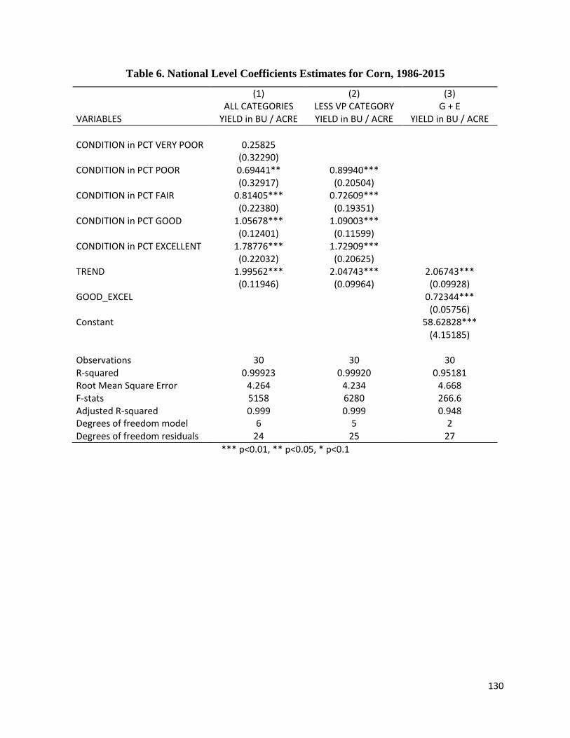
130

Table 6. National Level Coefficients Estimates for Corn, 1986-2015

*** p<0.01, ** p<0.05, * p<0.1

(1) (2) (3) ALL CATEGORIES LESS VP CATEGORY G + E VARIABLES YIELD in BU / ACRE YIELD in BU / ACRE YIELD in BU / ACRE

CONDITION in PCT VERY POOR 0.25825 (0.32290) CONDITION in PCT POOR 0.69441** 0.89940*** (0.32917) (0.20504) CONDITION in PCT FAIR 0.81405*** 0.72609*** (0.22380) (0.19351) CONDITION in PCT GOOD 1.05678*** 1.09003*** (0.12401) (0.11599) CONDITION in PCT EXCELLENT 1.78776*** 1.72909*** (0.22032) (0.20625) TREND 1.99562*** 2.04743*** 2.06743*** (0.11946) (0.09964) (0.09928) GOOD_EXCEL 0.72344*** (0.05756) Constant 58.62828*** (4.15185) Observations 30 30 30 R-squared 0.99923 0.99920 0.95181 Root Mean Square Error 4.264 4.234 4.668 F-stats 5158 6280 266.6 Adjusted R-squared 0.999 0.999 0.948 Degrees of freedom model 6 5 2 Degrees of freedom residuals 24 25 27

131

Table 7. National Level Coefficients Estimates for Soybeans, 1986-2015

(1) (2) (3) ALL CATEGORIES LESS VP CATEGORY G + E

VARIABLES YIELD in BU / ACRE YIELD in BU / ACRE YIELD in BU / ACRE

CONDITION in PCT VERY POOR 0.45444** (0.18404) CONDITION in PCT POOR -0.11369 0.34282**

(0.22195) (0.13475) CONDITION in PCT FAIR 0.39592*** 0.20909**

(0.11050) (0.08836) CONDITION in PCT GOOD 0.27610*** 0.37047*** (0.06648) (0.05968)

CONDITION in PCT EXCELLENT 0.63818*** 0.50015*** (0.11431) (0.10940)

TREND 0.41474*** 0.42886*** 0.43179*** (0.03398) (0.03676) (0.02411) GOOD_EXCEL 0.19270***

(0.01774) Constant 21.20737***

(1.03903) Observations 30 30 30

R-squared 0.99936 0.99919 0.94855 Root Mean Square Error 1.107 1.214 1.133

F-stats 6213 6192 248.9 Adjusted R-squared 0.999 0.999 0.945 Degrees of freedom model 6 5 2

Degrees of freedom residual 24 25 27

Standard errors in parentheses *** p<0.01, ** p<0.05, * p<0.1

132

Table 8. National Level Coefficients Estimates for Cotton Upland, 1986-2015

(1) (2) (3) ALL CATEGORIES LESS VP CATEGORY G + E VARIABLES YIELD in LB / ACRE YIELD in LB / ACRE YIELD in LB / ACRE

CONDITION in PCT VERY POOR 10.53722*** (2.55031) CONDITION in PCT POOR -2.82211 5.28728** (2.64857) (2.27943) CONDITION in PCT FAIR 5.76455*** 4.08978*** (1.11965) (1.33776) CONDITION in PCT GOOD 6.35718*** 6.64833*** (0.91399) (1.16824) CONDITION in PCT EXCELLENT 10.63446*** 9.274341*** (2.21515) (2.80771) TREND 8.99692*** 10.33065*** 9.9604*** (1.23782) (1.53165) (0.97591) GOOD_EXCEL 3.77058*** (0.71993) Constant 370.504*** (42.75642) Observations 30 30 30 R-squared 0.9974 0.99561 0.8043 Root Mean Squared Error 40.46 51.86 44.59 F-stats 1562 1139 55.49 Adjusted R-squared 0.997 0.995 0.79 Degrees of freedom model 6 5 2 Degrees of freedom residuals 24 25 27

Standard errors in parentheses *** p<0.01, ** p<0.05, * p<0.1

133

Table 9. National Level Coefficients Estimates for Winter Wheat, 1986-2015

(1) (2) (3) ALL CATEGORIES LESS VP CATEGORY G + E YIELD YIELD YIELD VARIABLES in BU / ACRE in BU / ACRE in BU / ACRE

CONDITION in PCT VERY POOR

0.24234**

(0.10599) CONDITION in PCT POOR 0.52388*** 0.82734*** (0.16758) (0.11062) CONDITION in PCT FAIR 0.11217 0.02237 (0.08700) (0.08394) CONDITION in PCT GOOD 0.53649*** 0.56309*** (0.06571) (0.06993) CONDITION in PCT EXCELLENT

0.45605*** 0.39876**

(0.13902) (0.14786) TREND 0.32104*** 0.34054*** 0.37700*** (0.05172) (0.05515) (0.04464) GOOD_EXCEL 0.18178*** (0.03193) Constant 27.79313*** (1.84235) Observations 30 30 30 R-squared 0.99824 0.99786 0.75757 Root Mean Squared Error 1.984 2.146 2.043 F-stats 2272 2331 42.19 Adjusted R-squared 0.998 0.997 0.740 Degrees of freedom model 6 5 2 Degrees of freedom residuals 24 25 27

Standard errors in parentheses *** p<0.01, ** p<0.05, * p<0.1

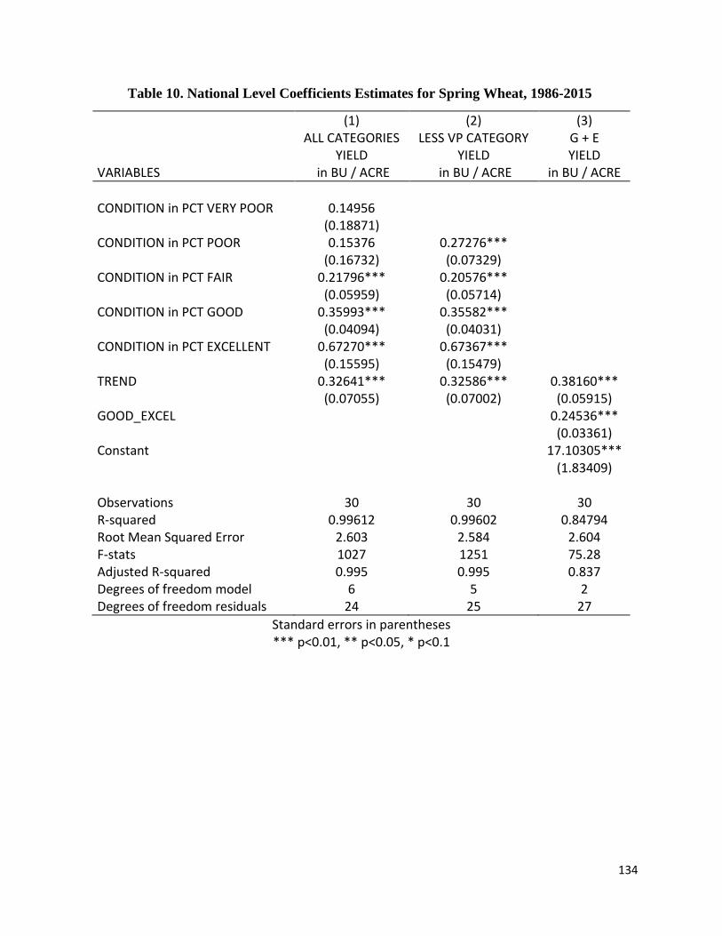
134

Table 10. National Level Coefficients Estimates for Spring Wheat, 1986-2015

(1) (2) (3) ALL CATEGORIES LESS VP CATEGORY G + E YIELD YIELD YIELD VARIABLES in BU / ACRE in BU / ACRE in BU / ACRE

CONDITION in PCT VERY POOR 0.14956 (0.18871) CONDITION in PCT POOR 0.15376 0.27276*** (0.16732) (0.07329) CONDITION in PCT FAIR 0.21796*** 0.20576*** (0.05959) (0.05714) CONDITION in PCT GOOD 0.35993*** 0.35582*** (0.04094) (0.04031) CONDITION in PCT EXCELLENT 0.67270*** 0.67367*** (0.15595) (0.15479) TREND 0.32641*** 0.32586*** 0.38160*** (0.07055) (0.07002) (0.05915) GOOD_EXCEL 0.24536*** (0.03361) Constant 17.10305*** (1.83409) Observations 30 30 30 R-squared 0.99612 0.99602 0.84794 Root Mean Squared Error 2.603 2.584 2.604 F-stats 1027 1251 75.28 Adjusted R-squared 0.995 0.995 0.837 Degrees of freedom model 6 5 2 Degrees of freedom residuals 24 25 27

Standard errors in parentheses *** p<0.01, ** p<0.05, * p<0.1

135

Table 11. Corn Yield Forecast Weekly Errors 2006-2015

REFERENCE PERIOD

G + E Categories Model All Categories Model Less VP Category Model

AVERAGE DATE

WEEK NUMBER

USDA Data Base

Model

Bias Adjusted

Prod Weights

3yr moving

avg

Prod Weights

5yr moving

avg

Prod Weights

3yr moving avg Bias Adjusted

Prod Weights

5yr moving avg Bias Adjusted

USDA Data

Bias Adjusted

Prod Weights

3yr moving

avg

Prod Weights

5yr moving

avg

Prod Weights

3yr moving avg Bias Adjusted

Prod Weights

5yr moving avg Bias Adjusted

USDA Data

Bias Adjusted

Prod Weights

3yr moving

avg

Prod Weights

5yr moving

avg

Prod Weights

3yr moving avg Bias Adjusted

Prod Weights

5yr moving avg Bias Adjusted

MAPE MAPE MAPE MAPE MAPE MAPE MAPE MAPE MAPE MAPE MAPE MAPE MAPE MAPE MAPE MAPE MAPE MAPE

Jun-2 WEEK #22

8.549 7.070 7.347 7.310 6.400 6.506 7.327 6.905 7.250 7.636 7.362 7.646 7.813 7.552 7.601 7.968 7.480 7.730

Jun-9 WEEK #23

8.139 6.969 7.114 6.980 6.166 6.231 7.162 6.679 6.936 7.261 6.891 7.226 7.588 7.325 7.330 7.576 7.007 7.241

Jun-16 WEEK #24

7.583 6.309 6.724 6.666 5.684 5.891 6.659 6.066 6.302 7.069 5.938 6.921 7.155 6.648 6.796 7.363 6.042 6.781

Jun-23 WEEK #25

7.090 6.017 6.414 6.356 5.499 5.583 6.582 5.950 6.508 6.559 5.767 5.970 6.921 6.500 6.947 6.863 5.868 6.041

Jun-30 WEEK #26

6.496 5.345 5.697 5.626 4.896 4.977 6.088 5.277 5.591 6.098 4.718 5.152 6.473 5.749 5.802 6.327 4.806 5.034

Jul-7 WEEK #27

5.969 4.808 5.055 4.971 4.460 4.521 5.686 4.995 5.172 5.211 4.120 4.883 5.816 5.320 5.142 5.139 4.174 4.826

Jul-14 WEEK #28

5.036 3.890 4.271 4.177 3.629 3.715 4.922 4.042 4.243 4.177 3.560 3.883 4.697 4.280 3.795 3.958 3.600 3.831

Jul-21 WEEK #29

4.273 3.490 3.673 3.606 3.125 3.255 4.594 3.851 3.956 3.836 3.272 3.650 4.157 3.946 3.428 3.377 3.302 3.609

Jul-28 WEEK #30

4.041 3.665 3.560 3.429 3.273 3.391 4.452 4.121 3.746 4.075 3.461 3.694 3.745 4.177 2.967 3.394 3.476 3.678

Aug-4 WEEK #31

3.926 3.776 3.504 3.450 3.311 3.306 4.469 4.124 3.782 3.633 3.073 3.175 3.488 4.120 2.804 2.998 3.069 3.179

Aug-11 WEEK #32

3.882 3.938 3.357 3.407 3.218 3.307 4.415 4.381 3.491 3.655 3.048 3.169 3.423 4.319 2.489 2.867 3.033 3.182

Aug-18 WEEK #33

3.535 3.794 3.133 3.115 3.064 3.092 4.297 4.463 3.456 3.324 3.124 2.880 3.250 4.388 2.350 2.476 3.051 2.866

Aug-25 WEEK #34

3.138 3.531 2.759 2.738 2.727 2.811 3.738 4.210 3.303 3.363 3.173 3.334 2.622 4.141 2.136 2.579 3.154 3.317

Sep-1 WEEK #35

2.849 3.492 2.651 2.672 2.881 2.770 3.481 4.254 3.579 3.031 3.678 3.127 2.345 4.185 2.593 2.123 3.661 3.114

Sep-8 WEEK #36

3.031 3.558 2.822 2.809 3.027 2.915 3.670 4.460 3.754 3.418 3.888 3.499 2.519 4.360 2.359 2.413 3.864 3.478

Sep-15 WEEK #37

3.274 3.810 2.908 2.982 3.024 3.050 3.817 4.528 3.592 3.647 3.734 3.764 2.715 4.444 2.421 2.731 3.717 3.747

Sep-22 WEEK #38

3.093 3.616 3.033 3.056 3.218 3.254 3.995 4.611 4.070 4.086 4.327 4.309 2.533 4.533 2.825 3.124 4.311 4.295

Sep-29 WEEK #39

3.233 3.429 3.023 3.098 3.022 3.042 3.939 4.359 3.999 3.828 3.863 3.761 2.807 4.320 2.762 2.909 3.873 3.753

AVERAGE 4.841 4.473 4.280 4.247 3.923 3.979 4.961 4.849 4.596 4.661 4.278 4.447 4.448 5.017 4.030 4.233 4.305 4.428

136

Table 12. Corn Yield Forecast Weekly Errors 2006-2015 MAPE RATIO

REFERENCE PERIOD

G + E Categories Model All Categories Model Less VP Category Model

AVERAGE DATE

WEEK NUMBER

USDA Data Base

Model

Bias Adjusted

Prod Weights

3yr moving

avg

Prod Weights

5yr moving

avg

Prod Weights

3yr moving avg Bias Adjusted

Prod Weights

5yr moving avg Bias Adjusted

USDA Data

Bias Adjusted

Prod Weights

3yr moving

avg

Prod Weights

5yr moving

avg

Prod Weights

3yr moving avg Bias Adjusted

Prod Weights

5yr moving avg Bias Adjusted

USDA Data

Bias Adjusted

Prod Weights

3yr moving

avg

Prod Weights

5yr moving

avg

Prod Weights

3yr moving avg Bias Adjusted

Prod Weights

5yr moving avg Bias Adjusted

MAPE MAPE MAPE MAPE MAPE MAPE MAPE MAPE MAPE MAPE MAPE MAPE MAPE MAPE MAPE MAPE MAPE MAPE

Jun-2 WEEK #22

1.000 0.827 0.859 0.855 0.749 0.761 0.857 0.808 0.848 0.893 0.861 0.894 0.914 0.883 0.889 0.932 0.875 0.904

Jun-9 WEEK #23

1.000 0.856 0.874 0.858 0.758 0.766 0.880 0.821 0.852 0.892 0.847 0.888 0.932 0.900 0.901 0.931 0.861 0.890

Jun-16 WEEK #24

1.000 0.832 0.887 0.879 0.750 0.777 0.878 0.800 0.831 0.932 0.783 0.913 0.943 0.877 0.896 0.971 0.797 0.894

Jun-23 WEEK #25

1.000 0.849 0.905 0.896 0.776 0.787 0.928 0.839 0.918 0.925 0.813 0.842 0.976 0.917 0.980 0.968 0.828 0.852

Jun-30 WEEK #26

1.000 0.823 0.877 0.866 0.754 0.766 0.937 0.812 0.861 0.939 0.726 0.793 0.996 0.885 0.893 0.974 0.740 0.775

Jul-7 WEEK #27

1.000 0.806 0.847 0.833 0.747 0.757 0.953 0.837 0.866 0.873 0.690 0.818 0.974 0.891 0.861 0.861 0.699 0.808

Jul-14 WEEK #28

1.000 0.772 0.848 0.829 0.721 0.738 0.977 0.803 0.842 0.829 0.707 0.771 0.933 0.850 0.754 0.786 0.715 0.761

Jul-21 WEEK #29

1.000 0.817 0.859 0.844 0.731 0.762 1.075 0.901 0.926 0.898 0.766 0.854 0.973 0.923 0.802 0.790 0.773 0.844

Jul-28 WEEK #30

1.000 0.907 0.881 0.849 0.810 0.839 1.102 1.020 0.927 1.008 0.857 0.914 0.927 1.034 0.734 0.840 0.860 0.910

Aug-4 WEEK #31

1.000 0.962 0.893 0.879 0.843 0.842 1.138 1.051 0.963 0.926 0.783 0.809 0.889 1.050 0.714 0.764 0.782 0.810

Aug-11 WEEK #32

1.000 1.014 0.865 0.878 0.829 0.852 1.137 1.129 0.899 0.942 0.785 0.816 0.882 1.113 0.641 0.739 0.781 0.820

Aug-18 WEEK #33

1.000 1.073 0.886 0.881 0.867 0.875 1.216 1.263 0.978 0.940 0.884 0.815 0.919 1.241 0.665 0.701 0.863 0.811

Aug-25 WEEK #34

1.000 1.125 0.879 0.873 0.869 0.896 1.191 1.342 1.053 1.072 1.011 1.063 0.836 1.320 0.681 0.822 1.005 1.057

Sep-1 WEEK #35

1.000 1.225 0.931 0.938 1.011 0.972 1.222 1.493 1.256 1.064 1.291 1.098 0.823 1.469 0.910 0.745 1.285 1.093

Sep-8 WEEK #36

1.000 1.174 0.931 0.927 0.999 0.962 1.211 1.472 1.239 1.128 1.283 1.155 0.831 1.439 0.778 0.796 1.275 1.148

Sep-15 WEEK #37

1.000 1.164 0.888 0.911 0.924 0.932 1.166 1.383 1.097 1.114 1.141 1.150 0.829 1.357 0.739 0.834 1.135 1.145

Sep-22 WEEK #38

1.000 1.169 0.981 0.988 1.040 1.052 1.292 1.491 1.316 1.321 1.399 1.393 0.819 1.466 0.913 1.010 1.394 1.389

Sep-29 WEEK #39

1.000 1.061 0.935 0.958 0.935 0.941 1.219 1.348 1.237 1.184 1.195 1.163 0.869 1.336 0.854 0.900 1.198 1.161

AVERAGE 1.000 0.970 0.890 0.886 0.840 0.849 1.077 1.089 0.995 0.993 0.935 0.953 0.904 1.108 0.811 0.854 0.937 0.948

137

Table 13. Corn Yield Forecast Weekly Errors 2006-2015

REFERENCE PERIOD

G + E Categories Model All Categories Model Less VP Category Model

AVERAGE DATE

WEEK NUMBER

USDA Data Base

Model

Bias Adjusted

Prod Weights

3yr moving

avg

Prod Weights

5yr moving

avg

Prod Weights

3yr moving avg Bias Adjusted

Prod Weights

5yr moving avg Bias Adjusted

USDA Data

Bias Adjusted

Prod Weights

3yr moving

avg

Prod Weights

5yr moving

avg

Prod Weights

3yr moving avg Bias Adjusted

Prod Weights

5yr moving avg Bias Adjusted

USDA Data

Bias Adjusted

Prod Weights

3yr moving

avg

Prod Weights

5yr moving

avg

Prod Weights

3yr moving avg Bias Adjusted

Prod Weights

5yr moving avg Bias Adjusted

RMSPE RMSPE RMSPE RMSPE RMSPE RMSPE RMSPE RMSPE RMSPE RMSPE RMSPE RMSPE RMSPE RMSPE RMSPE RMSPE RMSPE RMSPE

Jun-2 WEEK #22

13.208 12.028 12.095 12.086 10.989 11.056 11.507 11.582 11.193 11.606 9.906 11.820 12.540 12.013 11.775 12.112 10.560 11.827

Jun-9 WEEK #23

12.387 11.165 11.300 11.272 10.150 10.165 10.733 10.625 10.192 10.462 8.922 10.484 11.707 11.116 10.716 10.912 9.484 10.478

Jun-16 WEEK #24

11.701 10.387 10.620 10.656 9.432 9.406 10.066 9.728 9.232 9.731 7.864 9.411 11.067 10.179 9.808 10.203 8.344 9.392

Jun-23 WEEK #25

10.639 9.308 9.919 9.888 8.710 8.634 9.568 8.953 8.853 8.966 7.268 8.165 10.348 9.398 9.325 9.342 7.694 8.185

Jun-30 WEEK #26

9.459 7.957 8.839 8.667 7.345 7.365 8.639 7.548 7.597 7.989 5.657 6.699 9.228 7.976 7.907 8.247 6.060 6.687

Jul-7 WEEK #27

8.367 7.256 7.661 7.595 6.567 6.640 8.093 7.251 7.088 7.305 5.285 6.312 7.940 7.571 6.734 7.066 5.579 6.286

Jul-14 WEEK #28

6.830 5.844 6.383 6.363 5.514 5.467 6.981 6.147 5.909 5.939 4.581 4.953 6.306 6.397 5.104 5.514 4.790 4.926

Jul-21 WEEK #29

5.854 5.118 5.569 5.504 4.744 4.749 6.710 5.950 5.523 5.390 4.072 4.578 5.417 6.122 4.598 4.732 4.212 4.561

Jul-28 WEEK #30

5.565 5.073 5.240 5.063 4.672 4.713 6.690 6.135 5.509 5.563 4.466 4.730 5.065 6.235 4.054 4.676 4.543 4.719

Aug-8 WEEK #31

5.353 5.124 5.051 4.848 4.586 4.532 6.743 6.384 5.189 4.828 4.300 4.083 4.750 6.377 3.762 4.224 4.280 4.085

Aug-11 WEEK #32

5.242 5.332 4.814 4.735 4.624 4.601 6.681 6.652 5.148 4.938 4.626 4.345 4.658 6.592 3.461 3.983 4.520 4.346

Aug-18 WEEK #33

5.014 5.236 4.611 4.504 4.495 4.469 6.546 6.674 4.956 4.537 4.665 4.085 4.309 6.603 3.051 3.337 4.550 4.082

Aug-25 WEEK #34

4.593 4.971 4.334 4.192 4.311 4.249 6.162 6.518 4.899 4.438 4.804 4.199 3.796 6.454 3.030 3.563 4.690 4.194

Sep-1 WEEK #35

4.359 4.912 4.084 4.118 4.283 4.178 6.049 6.648 4.525 4.115 4.754 4.118 3.577 6.585 3.170 3.129 4.661 4.113

Sep-8 WEEK #36

4.373 4.944 4.308 4.265 4.492 4.334 6.036 6.758 5.077 4.482 5.348 4.467 3.501 6.668 2.912 3.317 5.203 4.460

Sep-15 WEEK #37

4.597 5.182 4.360 4.433 4.552 4.481 6.120 6.875 4.909 4.777 5.171 4.836 3.608 6.800 3.049 3.528 5.068 4.827

Sep-22 WEEK #38

4.494 5.025 4.495 4.433 4.690 4.595 6.359 7.021 5.234 4.931 5.644 5.141 3.370 6.957 3.170 3.719 5.550 5.131

Sep-29 WEEK #39

4.633 4.778 4.506 4.573 4.607 4.487 6.489 6.678 5.347 4.796 5.247 4.748 3.586 6.647 3.155 3.362 5.253 4.744

AVERAGE 7.037 6.647 6.566 6.511 6.042 6.007 7.565 7.451 6.466 6.377 5.699 5.954 6.376 7.594 5.488 5.831 5.836 5.947

138

Table 14. Corn Yield Forecast Weekly Errors 2006-2015 RMSPE RATIO

REFERENCE PERIOD

G + E Categories Model All Categories Model Less VP Category Model

AVERAGE DATE

WEEK NUMBER

USDA Data Base

Model

Bias Adjusted

Prod Weights

3yr moving

avg

Prod Weights

5yr moving

avg

Prod Weights

3yr moving avg Bias Adjusted

Prod Weights

5yr moving avg Bias Adjusted

USDA Data

Bias Adjusted

Prod Weights

3yr moving

avg

Prod Weights

5yr moving

avg

Prod Weights

3yr moving avg Bias Adjusted

Prod Weights

5yr moving avg Bias Adjusted

USDA Data

Bias Adjusted

Prod Weights

3yr moving

avg

Prod Weights

5yr moving

avg

Prod Weights

3yr moving avg Bias Adjusted

Prod Weights

5yr moving avg Bias Adjusted

RMSPE RMSPE RMSPE RMSPE RMSPE RMSPE RMSPE RMSPE RMSPE RMSPE RMSPE RMSPE RMSPE RMSPE RMSPE RMSPE RMSPE RMSPE

Jun-2 WEEK #22

1.000 0.911 0.916 0.915 0.832 0.837 0.871 0.877 0.847 0.879 0.750 0.895 0.949 0.910 0.891 0.917 0.800 0.895

Jun-9 WEEK #23

1.000 0.901 0.912 0.910 0.819 0.821 0.866 0.858 0.823 0.845 0.720 0.846 0.945 0.897 0.865 0.881 0.766 0.846

Jun-16 WEEK #24

1.000 0.888 0.908 0.911 0.806 0.804 0.860 0.831 0.789 0.832 0.672 0.804 0.946 0.870 0.838 0.872 0.713 0.803

Jun-23 WEEK #25

1.000 0.875 0.932 0.929 0.819 0.812 0.899 0.842 0.832 0.843 0.683 0.767 0.973 0.883 0.877 0.878 0.723 0.769

Jun-30 WEEK #26

1.000 0.841 0.934 0.916 0.777 0.779 0.913 0.798 0.803 0.845 0.598 0.708 0.976 0.843 0.836 0.872 0.641 0.707

Jul-7 WEEK #27

1.000 0.867 0.916 0.908 0.785 0.794 0.967 0.867 0.847 0.873 0.632 0.754 0.949 0.905 0.805 0.845 0.667 0.751

Jul-14 WEEK #28

1.000 0.856 0.935 0.932 0.807 0.800 1.022 0.900 0.865 0.870 0.671 0.725 0.923 0.937 0.747 0.807 0.701 0.721

Jul-21 WEEK #29

1.000 0.874 0.951 0.940 0.810 0.811 1.146 1.017 0.944 0.921 0.696 0.782 0.925 1.046 0.785 0.808 0.720 0.779

Jul-28 WEEK #30

1.000 0.912 0.942 0.910 0.840 0.847 1.202 1.103 0.990 1.000 0.803 0.850 0.910 1.120 0.728 0.840 0.816 0.848

Aug-8 WEEK #31

1.000 0.957 0.944 0.906 0.857 0.847 1.260 1.193 0.969 0.902 0.803 0.763 0.887 1.191 0.703 0.789 0.799 0.763

Aug-11 WEEK #32

1.000 1.017 0.918 0.903 0.882 0.878 1.275 1.269 0.982 0.942 0.883 0.829 0.889 1.258 0.660 0.760 0.862 0.829

Aug-18 WEEK #33

1.000 1.044 0.920 0.898 0.896 0.891 1.305 1.331 0.988 0.905 0.930 0.815 0.859 1.317 0.608 0.665 0.907 0.814

Aug-25 WEEK #34

1.000 1.082 0.943 0.913 0.938 0.925 1.341 1.419 1.067 0.966 1.046 0.914 0.826 1.405 0.660 0.776 1.021 0.913

Sep-1 WEEK #35

1.000 1.127 0.937 0.945 0.983 0.958 1.388 1.525 1.038 0.944 1.091 0.945 0.821 1.511 0.727 0.718 1.069 0.943

Sep-8 WEEK #36

1.000 1.131 0.985 0.975 1.027 0.991 1.380 1.546 1.161 1.025 1.223 1.022 0.801 1.525 0.666 0.759 1.190 1.020

Sep-15 WEEK #37

1.000 1.127 0.948 0.964 0.990 0.975 1.331 1.495 1.068 1.039 1.125 1.052 0.785 1.479 0.663 0.767 1.102 1.050

Sep-22 WEEK #38

1.000 1.118 1.000 0.987 1.044 1.023 1.415 1.562 1.165 1.097 1.256 1.144 0.750 1.548 0.705 0.828 1.235 1.142

Sep-29 WEEK #39

1.000 1.031 0.972 0.987 0.994 0.968 1.401 1.441 1.154 1.035 1.132 1.025 0.774 1.435 0.681 0.726 1.134 1.024

AVERAGE 1.000 0.976 0.940 0.930 0.884 0.876 1.158 1.160 0.963 0.931 0.873 0.869 0.883 1.171 0.747 0.806 0.881 0.868

139

Table 15. Soybean Yield Forecast Weekly Errors 2006-2015

REFERENCE PERIOD

G + E Categories Model All Categories Model Less VP Category Model

AVERAGE DATE

WEEK NUMBER

USDA Data Base

Model

Bias Adjusted

Prod Weights

3yr moving

avg

Prod Weights

5yr moving

avg

Prod Weights

3yr moving avg Bias Adjusted

Prod Weights

5yr moving avg Bias Adjusted

USDA Data

Bias Adjusted

Prod Weights

3yr moving

avg

Prod Weights

5yr moving

avg

Prod Weights

3yr moving avg Bias Adjusted

Prod Weights

5yr moving avg Bias Adjusted

USDA Data

Bias Adjusted

Prod Weights

3yr moving

avg

Prod Weights

5yr moving

avg

Prod Weights

3yr moving avg Bias Adjusted

Prod Weights

5yr moving avg Bias Adjusted

MAPE MAPE MAPE MAPE MAPE MAPE MAPE MAPE MAPE MAPE MAPE MAPE MAPE MAPE MAPE MAPE MAPE MAPE

Jun-16 WEEK #24

4.328 2.996 3.877 4.070 2.863 2.938 3.443 3.322 3.061 3.452 2.691 3.963 4.383 3.120 3.167 4.115 2.655 3.413

Jun-23 WEEK #25

4.219 2.911 3.941 4.000 2.683 2.861 3.404 2.806 3.190 3.191 2.572 3.489 4.194 3.029 3.390 3.948 2.326 2.971

Jun-30 WEEK #26

4.052 2.980 3.728 3.843 2.785 2.852 3.088 2.662 3.381 2.954 2.936 3.516 4.161 2.889 3.558 3.728 2.684 2.828

Jul-7 WEEK #27

3.679 3.259 3.684 3.702 3.360 3.430 3.667 3.177 3.932 3.886 3.499 4.208 3.698 3.458 4.036 4.151 3.305 3.813

Jul-14 WEEK #28

3.638 3.408 3.696 3.686 3.503 3.332 3.746 3.271 4.016 3.705 3.749 4.077 3.779 3.565 4.064 3.775 3.585 3.622

Jul-21 WEEK #29

3.879 3.523 3.842 3.744 3.478 3.655 4.051 3.643 3.951 4.254 3.804 4.643 4.210 3.904 4.038 4.429 3.652 4.232

Jul-28 WEEK #30

3.791 3.521 3.887 3.835 3.641 3.658 3.891 3.712 3.952 4.096 4.078 4.380 4.391 3.779 4.206 4.400 3.961 4.036

Aug-4 WEEK #31

3.795 3.622 3.756 3.786 3.701 3.817 3.578 3.337 3.922 3.932 4.067 4.113 4.325 3.495 4.138 4.533 4.008 3.890

Aug-11 WEEK #32

3.607 3.460 3.543 3.575 3.500 3.501 3.466 3.349 3.724 3.580 3.655 3.683 4.191 3.400 4.129 4.245 3.651 3.539

Aug-18 WEEK #33

3.016 2.957 3.159 3.180 3.089 3.135 3.005 2.905 3.375 3.416 3.381 3.421 3.633 2.962 3.819 3.939 3.381 3.365

Aug-25 WEEK #34

2.922 2.926 2.901 2.931 2.870 3.045 2.799 2.747 2.861 3.230 2.816 3.269 3.593 2.747 3.207 3.918 2.816 3.225

Sep-1 WEEK #35

2.683 2.692 2.623 2.627 2.530 2.725 2.384 2.264 2.836 2.955 2.878 3.112 3.160 2.264 3.097 3.647 2.879 3.102

Sep-8 WEEK #36

2.539 2.620 2.609 2.741 2.627 2.983 2.451 2.471 3.034 3.463 3.307 3.644 2.999 2.453 3.210 4.169 3.303 3.668

Sep-15 WEEK #37

2.475 2.667 2.441 2.605 2.689 2.777 2.739 2.586 3.077 2.683 3.214 2.929 3.036 2.601 3.178 3.505 3.210 2.962

Sep-22 WEEK #38

2.343 2.483 2.270 2.599 2.401 2.671 2.445 2.196 2.404 2.734 2.707 2.895 2.952 2.207 2.698 3.751 2.702 2.924

Sep-29 WEEK #39

2.211 2.340 2.323 2.484 2.308 2.546 2.170 2.226 2.629 2.932 2.778 3.088 2.877 2.208 2.831 3.427 2.775 3.108

AVERAGE 3.324 3.023 3.267 3.338 3.002 3.120 3.146 2.917 3.334 3.404 3.258 3.652 3.724 3.005 3.548 3.980 3.181 3.419

140

Table 16. Soybean Yield Forecast Weekly Errors 2006-2015 MAPE RATIO

REFERENCE PERIOD

G + E Categories Model All Categories Model Less VP Category Model

AVARAGE DATE

WEEK NUMBER

USDA Data Base

Model

Bias Adjusted

Prod Weights

3yr moving

avg

Prod Weights

5yr moving

avg

Prod Weights

3yr moving avg Bias Adjusted

Prod Weights

5yr moving avg Bias Adjusted

USDA Data

Bias Adjusted

Prod Weights

3yr moving

avg

Prod Weights

5yr moving

avg

Prod Weights

3yr moving avg Bias Adjusted

Prod Weights

5yr moving avg Bias Adjusted

USDA Data

Bias Adjusted

Prod Weights

3yr moving

avg

Prod Weights

5yr moving

avg

Prod Weights

3yr moving avg Bias Adjusted

Prod Weights

5yr moving avg Bias Adjusted

MAPE MAPE MAPE MAPE MAPE MAPE MAPE MAPE MAPE MAPE MAPE MAPE MAPE MAPE MAPE MAPE MAPE MAPE

Jun-16 WEEK #24

1.000 0.692 0.896 0.941 0.662 0.679 0.796 0.768 0.707 0.798 0.622 0.916 1.013 0.721 0.732 0.951 0.613 0.789

Jun-23 WEEK #25

1.000 0.690 0.934 0.948 0.636 0.678 0.807 0.665 0.756 0.756 0.609 0.827 0.994 0.718 0.803 0.936 0.551 0.704

Jun-30 WEEK #26

1.000 0.736 0.920 0.949 0.687 0.704 0.762 0.657 0.835 0.729 0.725 0.868 1.027 0.713 0.878 0.920 0.662 0.698

Jul-7 WEEK #27

1.000 0.886 1.001 1.006 0.913 0.932 0.997 0.864 1.069 1.056 0.951 1.144 1.005 0.940 1.097 1.128 0.898 1.037

Jul-14 WEEK #28

1.000 0.937 1.016 1.013 0.963 0.916 1.030 0.899 1.104 1.019 1.031 1.121 1.039 0.980 1.117 1.038 0.985 0.996

Jul-21 WEEK #29

1.000 0.908 0.990 0.965 0.897 0.942 1.044 0.939 1.018 1.097 0.981 1.197 1.085 1.006 1.041 1.142 0.941 1.091

Jul-28 WEEK #30

1.000 0.929 1.025 1.012 0.961 0.965 1.027 0.979 1.043 1.081 1.076 1.156 1.158 0.997 1.110 1.161 1.045 1.065

Aug-4 WEEK #31

1.000 0.954 0.990 0.998 0.975 1.006 0.943 0.879 1.033 1.036 1.072 1.084 1.139 0.921 1.090 1.194 1.056 1.025

Aug-11 WEEK #32

1.000 0.959 0.982 0.991 0.970 0.971 0.961 0.928 1.032 0.993 1.013 1.021 1.162 0.943 1.145 1.177 1.012 0.981

Aug-18 WEEK #33

1.000 0.980 1.048 1.055 1.024 1.040 0.996 0.963 1.119 1.133 1.121 1.134 1.205 0.982 1.267 1.306 1.121 1.116

Aug-25 WEEK #34

1.000 1.001 0.993 1.003 0.982 1.042 0.958 0.940 0.979 1.105 0.964 1.119 1.229 0.940 1.098 1.341 0.964 1.103

Sep-1 WEEK #35

1.000 1.003 0.978 0.979 0.943 1.016 0.889 0.844 1.057 1.102 1.073 1.160 1.178 0.844 1.154 1.359 1.073 1.156

Sep-8 WEEK #36

1.000 1.032 1.027 1.080 1.035 1.175 0.965 0.973 1.195 1.364 1.302 1.435 1.181 0.966 1.264 1.642 1.301 1.445

Sep-15 WEEK #37

1.000 1.078 0.986 1.052 1.087 1.122 1.107 1.045 1.243 1.084 1.299 1.183 1.227 1.051 1.284 1.416 1.297 1.197

Sep-22 WEEK #38

1.000 1.060 0.969 1.109 1.025 1.140 1.044 0.937 1.026 1.167 1.155 1.235 1.260 0.942 1.152 1.601 1.153 1.248

Sep-29 WEEK #39

1.000 1.058 1.051 1.123 1.044 1.152 0.982 1.007 1.189 1.326 1.257 1.397 1.301 0.999 1.281 1.550 1.255 1.406

AVERAGE 1.000 0.932 0.988 1.014 0.925 0.967 0.957 0.893 1.025 1.053 1.016 1.125 1.138 0.916 1.094 1.241 0.996 1.066

141

Table 17. Soybean Yield Forecast Weekly Errors 2006-2015

REFERENCE PERIOD

G + E Categories Model All Categories Model Less VP Category Model

AVERAGE DATE

WEEK NUMBER

USDA Data Base

Model

Bias Adjusted

Prod Weights

3yr moving

avg

Prod Weights

5yr moving

avg

Prod Weights

3yr moving avg Bias Adjusted

Prod Weights

5yr moving avg Bias Adjusted

USDA Data

Bias Adjusted

Prod Weights

3yr moving

avg

Prod Weights

5yr moving

avg

Prod Weights

3yr moving avg Bias Adjusted

Prod Weights

5yr moving avg Bias Adjusted

USDA Data

Bias Adjusted

Prod Weights

3yr moving

avg

Prod Weights

5yr moving

avg

Prod Weights

3yr moving avg Bias Adjusted

Prod Weights

5yr moving avg Bias Adjusted

RMSPE RMSPE RMSPE RMSPE RMSPE RMSPE RMSPE RMSPE RMSPE RMSPE RMSPE RMSPE RMSPE RMSPE RMSPE RMSPE RMSPE RMSPE

Jun-16 WEEK #24

5.191 3.531 4.651 4.771 3.325 3.572 4.075 3.680 3.578 3.974 3.286 4.634 5.049 3.722 3.688 4.496 3.245 3.970

Jun-23 WEEK #25

4.888 3.429 4.545 4.462 3.206 3.358 4.074 3.390 3.897 3.942 3.372 4.437 4.965 3.586 3.885 4.319 3.226 3.782

Jun-30 WEEK #26

4.812 3.624 4.461 4.469 3.539 3.536 4.051 3.370 4.265 3.887 3.621 4.507 5.074 3.684 4.372 4.336 3.458 3.784

Jul-7 WEEK #27

4.578 3.852 4.539 4.463 4.012 3.973 4.333 3.885 4.713 4.592 4.210 4.969 4.794 4.116 4.778 4.739 4.114 4.498

Jul-14 WEEK #28

4.359 3.896 4.451 4.345 4.199 3.954 4.378 4.161 4.765 4.395 4.620 4.760 4.622 4.220 4.753 4.546 4.463 4.320

Jul-21 WEEK #29

4.549 4.222 4.530 4.366 4.280 4.383 4.571 4.462 4.852 5.047 4.744 5.400 5.041 4.465 4.929 5.342 4.592 5.007

Jul-28 WEEK #30

4.523 4.360 4.702 4.584 4.609 4.510 4.522 4.509 5.122 4.814 5.042 5.181 5.333 4.474 5.402 5.310 4.938 4.829

Aug-8 WEEK #31

4.642 4.490 4.647 4.563 4.595 4.610 4.537 4.414 4.992 4.812 4.913 4.924 5.298 4.418 5.277 5.348 4.864 4.741

Aug-11 WEEK #32

4.492 4.332 4.560 4.468 4.492 4.496 4.355 4.268 4.811 4.754 4.676 4.811 5.266 4.281 5.165 5.305 4.653 4.696

Aug-18 WEEK #33

4.040 3.971 4.248 4.166 4.149 4.168 4.072 4.004 4.481 4.474 4.426 4.480 4.928 4.018 4.873 5.150 4.425 4.439

Aug-25 WEEK #34

3.854 3.858 3.883 3.800 3.847 3.914 3.677 3.662 3.993 3.895 3.922 3.928 4.906 3.666 4.395 4.866 3.921 3.893

Sep-1 WEEK #35

3.354 3.410 3.412 3.329 3.390 3.449 3.188 3.144 3.824 3.921 3.818 3.932 4.264 3.144 4.409 4.435 3.820 3.917

Sep-8 WEEK #36

3.222 3.388 3.422 3.414 3.481 3.581 3.410 3.399 4.056 4.189 4.139 4.136 3.946 3.399 4.325 4.732 4.143 4.180

Sep-15 WEEK #37

3.250 3.450 3.193 3.198 3.402 3.344 3.530 3.398 3.794 3.519 3.879 3.448 3.950 3.420 3.959 3.880 3.873 3.512

Sep-22 WEEK #38

3.108 3.301 2.969 3.166 3.100 3.150 3.116 3.042 3.294 3.319 3.376 3.358 3.708 3.050 3.453 3.994 3.374 3.398

Sep-29 WEEK #39

3.077 3.213 3.052 3.049 3.004 3.146 3.048 3.078 3.359 3.641 3.386 3.604 3.690 3.078 3.565 3.706 3.389 3.636

AVERAGE 4.121 3.770 4.079 4.038 3.789 3.821 3.934 3.742 4.237 4.198 4.089 4.407 4.677 3.796 4.452 4.656 4.031 4.163

142

Table 18. Soybean Yield Forecast Weekly Errors 2006-2015 RMSPE RATIO

REFERENCE PERIOD

G + E Categories Model All Categories Model Less VP Category Model

AVERAGE DATE

WEEK NUMBER

USDA Data

Bias Adjusted

Prod Weights

3yr moving

avg

Prod Weights

5yr moving

avg

Prod Weights

3yr moving avg Bias Adjusted

Prod Weights

5yr moving avg Bias Adjusted

USDA Data

Bias Adjusted

Prod Weights

3yr moving

avg

Prod Weights

5yr moving

avg

Prod Weights

3yr moving avg Bias Adjusted

Prod Weights

5yr moving avg Bias Adjusted

USDA Data

Bias Adjusted

Prod Weights

3yr moving

avg

Prod Weights

5yr moving

avg

Prod Weights

3yr moving avg Bias Adjusted

Prod Weights

5yr moving avg Bias Adjusted

RMSPE RMSPE RMSPE RMSPE RMSPE RMSPE RMSPE RMSPE RMSPE RMSPE RMSPE RMSPE RMSPE RMSPE RMSPE RMSPE RMSPE RMSPE

Jun-16 WEEK #24

1.000 0.680 0.896 0.919 0.641 0.688 0.785 0.709 0.689 0.766 0.633 0.893 0.973 0.717 0.710 0.866 0.625 0.765

Jun-23 WEEK #25

1.000 0.701 0.930 0.913 0.656 0.687 0.833 0.694 0.797 0.806 0.690 0.908 1.016 0.734 0.795 0.883 0.660 0.774

Jun-30 WEEK #26

1.000 0.753 0.927 0.929 0.736 0.735 0.842 0.700 0.886 0.808 0.752 0.937 1.055 0.766 0.909 0.901 0.719 0.786

Jul-7 WEEK #27

1.000 0.841 0.991 0.975 0.876 0.868 0.947 0.849 1.029 1.003 0.919 1.085 1.047 0.899 1.044 1.035 0.899 0.982

Jul-14 WEEK #28

1.000 0.894 1.021 0.997 0.963 0.907 1.004 0.955 1.093 1.008 1.060 1.092 1.060 0.968 1.090 1.043 1.024 0.991

Jul-21 WEEK #29

1.000 0.928 0.996 0.960 0.941 0.964 1.005 0.981 1.067 1.110 1.043 1.187 1.108 0.982 1.084 1.175 1.010 1.101

Jul-28 WEEK #30

1.000 0.964 1.040 1.013 1.019 0.997 1.000 0.997 1.132 1.064 1.115 1.145 1.179 0.989 1.194 1.174 1.092 1.068

Aug-8 WEEK #31

1.000 0.967 1.001 0.983 0.990 0.993 0.977 0.951 1.075 1.036 1.058 1.061 1.141 0.952 1.137 1.152 1.048 1.021

Aug-11 WEEK #32

1.000 0.965 1.015 0.995 1.000 1.001 0.970 0.950 1.071 1.058 1.041 1.071 1.172 0.953 1.150 1.181 1.036 1.045

Aug-18 WEEK #33

1.000 0.983 1.051 1.031 1.027 1.032 1.008 0.991 1.109 1.107 1.095 1.109 1.220 0.995 1.206 1.275 1.095 1.099

Aug-25 WEEK #34

1.000 1.001 1.007 0.986 0.998 1.015 0.954 0.950 1.036 1.011 1.018 1.019 1.273 0.951 1.140 1.263 1.017 1.010

Sep-1 WEEK #35

1.000 1.017 1.017 0.992 1.011 1.028 0.951 0.938 1.140 1.169 1.138 1.172 1.271 0.938 1.314 1.322 1.139 1.168

Sep-8 WEEK #36

1.000 1.051 1.062 1.060 1.080 1.111 1.058 1.055 1.259 1.300 1.285 1.284 1.225 1.055 1.342 1.469 1.286 1.297

Sep-15 WEEK #37

1.000 1.062 0.983 0.984 1.047 1.029 1.086 1.046 1.167 1.083 1.194 1.061 1.215 1.052 1.218 1.194 1.192 1.081

Sep-22 WEEK #38

1.000 1.062 0.955 1.019 0.997 1.013 1.002 0.979 1.060 1.068 1.086 1.080 1.193 0.981 1.111 1.285 1.085 1.093

Sep-29 WEEK #39

1.000 1.044 0.992 0.991 0.976 1.023 0.991 1.000 1.092 1.184 1.100 1.171 1.199 1.000 1.159 1.205 1.102 1.182

AVERAGE 1.000 0.932 0.993 0.984 0.935 0.943 0.963 0.921 1.044 1.036 1.014 1.080 1.147 0.933 1.100 1.151 1.002 1.029

143

Table 19. Cotton, Upland Yield Forecast Weekly Errors 2006-2015

REFERENCE PERIOD

G + E Categories Model All Categories Model Less VP Category Model

AVERAGE DATE

WEEK NUMBER

USDA Data Base

Model

Bias Adjusted

Prod Weights

3yr moving

avg

Prod Weights

5yr moving

avg

Prod Weights

3yr moving avg Bias Adjusted

Prod Weights

5yr moving avg Bias Adjusted

USDA Data

Bias Adjusted

Prod Weights

3yr moving

avg

Prod Weights

5yr moving

avg

Prod Weights

3yr moving avg Bias Adjusted

Prod Weights

5yr moving avg Bias Adjusted

USDA Data

Bias Adjusted

Prod Weights

3yr moving

avg

Prod Weights

5yr moving

avg

Prod Weights

3yr moving avg Bias Adjusted

Prod Weights

5yr moving avg Bias Adjusted

MAPE MAPE MAPE MAPE MAPE MAPE MAPE MAPE MAPE MAPE MAPE MAPE MAPE MAPE MAPE MAPE MAPE MAPE

Jun-16 WEEK #24

7.130 7.122 7.554 7.467 7.356 7.396 8.384 8.297 10.829 11.270 8.881 9.284 10.267 8.297 13.104 13.518 8.886 9.155

Jun-23 WEEK #25

7.414 7.400 7.874 7.744 7.841 7.906 7.223 7.100 10.507 10.823 9.347 9.119 9.651 7.100 12.884 12.921 9.351 9.027

Jun-30 WEEK #26

7.642 7.833 8.132 8.007 8.228 8.432 7.636 7.571 9.711 9.959 8.779 8.836 9.284 7.571 12.461 12.675 8.783 8.748

Jul-7 WEEK #27

7.831 8.009 8.413 8.237 8.366 8.462 8.172 7.773 9.698 9.807 8.544 8.846 9.436 7.773 12.050 12.387 8.547 8.771

Jul-14 WEEK #28

7.700 7.765 8.311 8.132 8.175 8.319 7.831 7.710 9.480 9.576 8.492 8.573 9.188 7.710 11.825 12.076 8.496 8.483

Jul-21 WEEK #29

7.823 7.797 8.448 8.160 8.292 8.205 8.947 8.674 9.972 9.584 8.995 8.737 9.707 8.674 11.941 11.981 8.999 8.655

Jul-28 WEEK #30

7.938 7.913 8.189 8.133 8.156 8.240 9.159 8.893 9.741 9.791 9.033 9.083 10.077 8.893 11.651 11.964 9.036 9.002

Aug-4 WEEK #31

8.239 8.216 8.475 8.425 8.438 8.341 8.984 8.720 10.267 9.909 9.722 9.531 10.551 8.720 12.554 12.158 9.725 9.454

Aug-11 WEEK #32

7.890 7.869 8.129 8.005 7.921 8.052 8.725 8.449 10.036 9.926 9.514 9.545 10.097 8.449 12.075 12.051 9.516 9.495

Aug-18 WEEK #33

8.086 8.066 8.240 8.300 8.094 8.357 9.123 8.887 10.214 10.217 9.707 9.866 10.774 8.887 12.523 12.609 9.708 9.828

Aug-25 WEEK #34

8.031 8.016 8.139 8.019 8.171 8.204 8.855 8.641 10.171 9.942 9.728 9.580 10.870 8.641 12.641 12.513 9.729 9.555

Sep-1 WEEK #35

7.692 7.679 8.024 7.953 8.117 8.136 8.761 8.687 9.883 9.631 9.502 9.361 10.351 8.687 12.339 12.074 9.502 9.346

Sep-8 WEEK #36

7.639 7.630 8.264 8.080 8.122 8.084 8.395 8.306 9.629 9.687 9.208 9.315 10.468 8.306 12.073 12.168 9.208 9.307

Sep-15 WEEK #37

7.642 7.640 8.382 8.093 8.184 8.279 8.148 8.104 9.492 9.088 9.194 8.828 10.289 8.104 11.977 11.671 9.194 8.822

Sep-22 WEEK #38

7.191 7.192 7.734 7.665 7.610 7.792 8.296 8.326 8.705 8.764 8.422 8.560 10.049 8.326 11.043 11.369 8.422 8.558

Sep-29 WEEK #39

6.780 6.782 7.373 7.163 7.259 7.350 7.804 7.868 8.874 8.532 8.730 8.427 9.513 7.868 11.176 10.855 8.730 8.417

Oct-20 WEEK #42

6.169 6.169 6.260 6.138 6.393 6.250 6.475 6.697 7.166 6.894 7.251 6.933 8.577 6.697 9.339 9.056 7.255 6.930

AVERAGE 7.579 7.594 7.997 7.866 7.925 7.988 8.289 8.159 9.669 9.612 9.003 8.966 9.950 8.159 11.980 12.003 9.005 8.915

144

Table 20. Cotton, Upland Yield Forecast Weekly Errors 2006-2015 MAPE RATIO

REFERENCE PERIOD

G + E Categories Model All Categories Model Less VP Category Model

AVERAGE DATE

WEEK NUMBER

USDA Data Base

Model

Bias Adjusted

Prod Weights

3yr moving

avg

Prod Weights

5yr moving

avg

Prod Weights

3yr moving avg Bias Adjusted

Prod Weights

5yr moving avg Bias Adjusted

USDA Data

Bias Adjusted

Prod Weights

3yr moving

avg

Prod Weights

5yr moving

avg

Prod Weights

3yr moving avg Bias Adjusted

Prod Weights

5yr moving avg Bias Adjusted

USDA Data

Bias Adjusted

Prod Weights

3yr moving

avg

Prod Weights

5yr moving

avg

Prod Weights

3yr moving avg Bias Adjusted

Prod Weights

5yr moving avg Bias Adjusted

MAPE MAPE MAPE MAPE MAPE MAPE MAPE MAPE MAPE MAPE MAPE MAPE MAPE MAPE MAPE MAPE MAPE MAPE

Jun-16 WEEK #24

1.000 0.999 1.059 1.047 1.032 1.037 1.176 1.164 1.519 1.581 1.246 1.302 1.440 1.164 1.838 1.896 1.246 1.284

Jun-23 WEEK #25

1.000 0.998 1.062 1.044 1.057 1.066 0.974 0.958 1.417 1.460 1.261 1.230 1.302 0.958 1.738 1.743 1.261 1.217

Jun-30 WEEK #26

1.000 1.025 1.064 1.048 1.077 1.103 0.999 0.991 1.271 1.303 1.149 1.156 1.215 0.991 1.631 1.659 1.149 1.145

Jul-7 WEEK #27

1.000 1.023 1.074 1.052 1.068 1.081 1.043 0.993 1.238 1.252 1.091 1.130 1.205 0.993 1.539 1.582 1.091 1.120

Jul-14 WEEK #28

1.000 1.008 1.079 1.056 1.062 1.080 1.017 1.001 1.231 1.244 1.103 1.113 1.193 1.001 1.536 1.568 1.103 1.102

Jul-21 WEEK #29

1.000 0.997 1.080 1.043 1.060 1.049 1.144 1.109 1.275 1.225 1.150 1.117 1.241 1.109 1.526 1.531 1.150 1.106

Jul-28 WEEK #30

1.000 0.997 1.032 1.025 1.027 1.038 1.154 1.120 1.227 1.233 1.138 1.144 1.269 1.120 1.468 1.507 1.138 1.134

Aug-8 WEEK #31

1.000 0.997 1.029 1.023 1.024 1.012 1.090 1.058 1.246 1.203 1.180 1.157 1.281 1.058 1.524 1.476 1.180 1.147

Aug-11 WEEK #32

1.000 0.997 1.030 1.015 1.004 1.020 1.106 1.071 1.272 1.258 1.206 1.210 1.280 1.071 1.530 1.527 1.206 1.203

Aug-18 WEEK #33

1.000 0.998 1.019 1.026 1.001 1.033 1.128 1.099 1.263 1.264 1.200 1.220 1.332 1.099 1.549 1.559 1.201 1.215

Aug-25 WEEK #34

1.000 0.998 1.013 0.998 1.017 1.022 1.103 1.076 1.267 1.238 1.211 1.193 1.353 1.076 1.574 1.558 1.211 1.190

Sep-1 WEEK #35

1.000 0.998 1.043 1.034 1.055 1.058 1.139 1.129 1.285 1.252 1.235 1.217 1.346 1.129 1.604 1.570 1.235 1.215

Sep-8 WEEK #36

1.000 0.999 1.082 1.058 1.063 1.058 1.099 1.087 1.261 1.268 1.205 1.219 1.370 1.087 1.581 1.593 1.206 1.218

Sep-15 WEEK #37

1.000 1.000 1.097 1.059 1.071 1.083 1.066 1.060 1.242 1.189 1.203 1.155 1.346 1.060 1.567 1.527 1.203 1.154

Sep-22 WEEK #38

1.000 1.000 1.076 1.066 1.058 1.084 1.154 1.158 1.211 1.219 1.171 1.190 1.398 1.158 1.536 1.581 1.171 1.190

Sep-29 WEEK #39

1.000 1.000 1.088 1.057 1.071 1.084 1.151 1.161 1.309 1.259 1.288 1.243 1.403 1.161 1.648 1.601 1.288 1.242

Oct-20 WEEK #42

1.000 1.000 1.015 0.995 1.036 1.013 1.050 1.086 1.162 1.118 1.176 1.124 1.390 1.086 1.514 1.468 1.176 1.123

AVERAGE 1.000 1.002 1.055 1.038 1.046 1.054 1.094 1.078 1.276 1.268 1.189 1.184 1.316 1.078 1.582 1.585 1.189 1.177

145

Table 21. Cotton, Upland Yield Forecast Weekly Errors 2006-2015

REFERENCE PERIOD

G + E Categories Model All Categories Model Less VP Category Model

AVERAGE DATE

WEEK NUMBER

USDA Data Base

Model

Bias Adjusted

Prod Weights

3yr moving

avg

Prod Weights

5yr moving

avg

Prod Weights

3yr moving avg Bias Adjusted

Prod Weights

5yr moving avg Bias Adjusted

USDA Data

Bias Adjusted

Prod Weights

3yr moving

avg

Prod Weights

5yr moving

avg

Prod Weights

3yr moving avg Bias Adjusted

Prod Weights

5yr moving avg Bias Adjusted

USDA Data

Bias Adjusted

Prod Weights

3yr moving

avg

Prod Weights

5yr moving

avg

Prod Weights

3yr moving avg Bias Adjusted

Prod Weights

5yr moving avg Bias Adjusted

RMSPE RMSPE RMSPE RMSPE RMSPE RMSPE RMSPE RMSPE RMSPE RMSPE RMSPE RMSPE RMSPE RMSPE RMSPE RMSPE RMSPE RMSPE

Jun-16 WEEK #24

8.743 8.748 9.006 8.974 8.794 8.807 9.903 9.884 12.629 12.894 10.481 10.912 12.003 9.884 15.529 15.782 10.425 10.730

Jun-23 WEEK #25

8.903 8.970 9.309 9.202 9.355 9.543 9.317 9.318 12.329 12.356 10.585 10.849 11.593 9.318 14.827 14.950 10.549 10.693

Jun-30 WEEK #26

8.979 9.097 9.438 9.342 9.631 9.746 9.066 9.078 12.046 11.848 10.552 10.605 11.675 9.078 15.023 14.833 10.500 10.452

Jul-7 WEEK #27

9.228 9.326 9.718 9.516 9.752 9.787 9.675 9.596 11.624 11.779 9.986 10.370 11.700 9.596 14.461 14.588 9.968 10.234

Jul-14 WEEK #28

9.207 9.309 9.773 9.717 9.787 9.834 9.415 9.464 11.671 11.505 10.372 10.584 11.708 9.464 14.311 14.195 10.325 10.414

Jul-21 WEEK #29

9.289 9.391 9.918 9.665 9.917 9.912 10.151 9.992 12.105 11.754 10.877 10.880 12.006 9.992 14.535 14.319 10.839 10.715

Jul-28 WEEK #30

9.318 9.385 9.681 9.551 9.746 9.760 10.320 10.159 11.705 11.923 10.802 11.077 12.114 10.159 14.244 14.494 10.790 10.921

Aug-8 WEEK #31

9.517 9.571 9.764 9.649 9.786 9.719 10.032 9.907 12.044 11.543 11.225 10.971 12.355 9.907 14.671 14.158 11.228 10.825

Aug-11 WEEK #32

9.154 9.265 9.491 9.381 9.538 9.650 10.027 9.871 11.557 11.611 10.880 11.101 11.963 9.871 13.872 13.967 10.873 11.006

Aug-18 WEEK #33

9.340 9.392 9.575 9.627 9.537 9.753 10.284 10.237 11.596 11.646 10.918 11.200 12.281 10.237 14.051 14.236 10.912 11.131

Aug-25 WEEK #34

9.218 9.268 9.393 9.276 9.451 9.420 9.891 9.760 11.476 11.303 10.869 10.809 12.272 9.760 14.225 14.107 10.865 10.764

Sep-1 WEEK #35

8.940 8.972 9.364 9.263 9.492 9.491 9.884 9.823 11.335 11.091 10.823 10.737 11.558 9.823 13.836 13.542 10.821 10.710

Sep-8 WEEK #36

8.829 8.851 9.508 9.279 9.452 9.359 9.246 9.232 11.023 10.894 10.559 10.518 11.655 9.232 13.543 13.498 10.556 10.504

Sep-15 WEEK #37

8.800 8.804 9.500 9.148 9.315 9.289 9.134 9.105 10.719 10.386 10.373 10.083 11.480 9.105 13.285 13.029 10.369 10.073

Sep-22 WEEK #38

8.490 8.488 8.876 8.762 8.788 8.863 9.310 9.346 10.188 10.190 9.916 9.893 11.200 9.346 12.500 12.702 9.915 9.890

Sep-29 WEEK #39

8.057 8.055 8.613 8.284 8.457 8.389 8.812 8.864 9.973 9.647 9.827 9.546 10.527 8.864 12.266 11.918 9.821 9.531

Oct-20 WEEK #42

7.305 7.300 7.420 7.292 7.643 7.359 7.313 7.441 8.557 8.090 8.690 8.154 9.614 7.441 10.570 10.075 8.692 8.149

AVERAGE 8.901 8.953 9.314 9.172 9.320 9.334 9.517 9.475 11.328 11.204 10.455 10.488 11.630 9.475 13.867 13.788 10.438 10.397

146

Table 22. Cotton, Upland Yield Forecast Weekly Errors 2006-2015 RMSPE RATIO

REFERENCE PERIOD

G + E Categories Model All Categories Model Less VP Category Model

AVERAGE DATE

WEEK NUMBER

USDA Data Base

Model

Bias Adjusted

Prod Weights

3yr moving

avg

Prod Weights

5yr moving

avg

Prod Weights

3yr moving avg Bias Adjusted

Prod Weights

5yr moving avg Bias Adjusted

USDA Data

Bias Adjusted

Prod Weights

3yr moving

avg

Prod Weights

5yr moving

avg

Prod Weights

3yr moving avg Bias Adjusted

Prod Weights

5yr moving avg Bias Adjusted

USDA Data

Bias Adjusted

Prod Weights

3yr moving

avg

Prod Weights

5yr moving

avg

Prod Weights

3yr moving avg Bias Adjusted

Prod Weights

5yr moving avg Bias Adjusted

RMSPE RMSPE RMSPE RMSPE RMSPE RMSPE RMSPE RMSPE RMSPE RMSPE RMSPE RMSPE RMSPE RMSPE RMSPE RMSPE RMSPE RMSPE

Jun-16 WEEK #24

1.000 1.001 1.030 1.026 1.006 1.007 1.133 1.131 1.444 1.475 1.199 1.248 1.373 1.131 1.776 1.805 1.192 1.227

Jun-23 WEEK #25

1.000 1.008 1.046 1.034 1.051 1.072 1.047 1.047 1.385 1.388 1.189 1.219 1.302 1.047 1.665 1.679 1.185 1.201

Jun-30 WEEK #26

1.000 1.013 1.051 1.040 1.073 1.085 1.010 1.011 1.342 1.320 1.175 1.181 1.300 1.011 1.673 1.652 1.169 1.164

Jul-7 WEEK #27

1.000 1.011 1.053 1.031 1.057 1.061 1.048 1.040 1.260 1.277 1.082 1.124 1.268 1.040 1.567 1.581 1.080 1.109

Jul-14 WEEK #28

1.000 1.011 1.061 1.055 1.063 1.068 1.023 1.028 1.268 1.250 1.126 1.150 1.272 1.028 1.554 1.542 1.121 1.131

Jul-21 WEEK #29

1.000 1.011 1.068 1.040 1.068 1.067 1.093 1.076 1.303 1.265 1.171 1.171 1.292 1.076 1.565 1.541 1.167 1.153

Jul-28 WEEK #30

1.000 1.007 1.039 1.025 1.046 1.047 1.108 1.090 1.256 1.279 1.159 1.189 1.300 1.090 1.529 1.555 1.158 1.172

Aug-8 WEEK #31

1.000 1.006 1.026 1.014 1.028 1.021 1.054 1.041 1.266 1.213 1.179 1.153 1.298 1.041 1.542 1.488 1.180 1.137

Aug-11 WEEK #32

1.000 1.012 1.037 1.025 1.042 1.054 1.095 1.078 1.263 1.268 1.189 1.213 1.307 1.078 1.515 1.526 1.188 1.202

Aug-18 WEEK #33

1.000 1.006 1.025 1.031 1.021 1.044 1.101 1.096 1.242 1.247 1.169 1.199 1.315 1.096 1.504 1.524 1.168 1.192

Aug-25 WEEK #34

1.000 1.005 1.019 1.006 1.025 1.022 1.073 1.059 1.245 1.226 1.179 1.173 1.331 1.059 1.543 1.530 1.179 1.168

Sep-1 WEEK #35

1.000 1.004 1.047 1.036 1.062 1.062 1.106 1.099 1.268 1.241 1.211 1.201 1.293 1.099 1.548 1.515 1.210 1.198

Sep-8 WEEK #36

1.000 1.002 1.077 1.051 1.071 1.060 1.047 1.046 1.249 1.234 1.196 1.191 1.320 1.046 1.534 1.529 1.196 1.190

Sep-15 WEEK #37

1.000 1.000 1.080 1.039 1.058 1.056 1.038 1.035 1.218 1.180 1.179 1.146 1.304 1.035 1.510 1.481 1.178 1.145

Sep-22 WEEK #38

1.000 1.000 1.045 1.032 1.035 1.044 1.097 1.101 1.200 1.200 1.168 1.165 1.319 1.101 1.472 1.496 1.168 1.165

Sep-29 WEEK #39

1.000 1.000 1.069 1.028 1.050 1.041 1.094 1.100 1.238 1.197 1.220 1.185 1.307 1.100 1.522 1.479 1.219 1.183

Oct-20 WEEK #42

1.000 0.999 1.016 0.998 1.046 1.007 1.001 1.019 1.171 1.107 1.190 1.116 1.316 1.019 1.447 1.379 1.190 1.116

AVERAGE 1.000 1.006 1.046 1.030 1.047 1.048 1.069 1.064 1.271 1.257 1.175 1.178 1.307 1.064 1.557 1.547 1.173 1.168

147

Table 23. Winter Wheat Yield Forecast Weekly Errors 2006-2015

REFERENCE PERIOD

G + E Categories Model All Categories Model Less VP Category Model

AVERAGE DATE

WEEK NUMBER

USDA Data Base

Model

Bias Adjusted

Prod Weights

3yr moving

avg

Prod Weights

5yr moving

avg

Prod Weights

3yr moving avg Bias Adjusted

Prod Weights

5yr moving avg Bias Adjusted

USDA Data

Bias Adjusted

Prod Weights

3yr moving

avg

Prod Weights

5yr moving

avg

Prod Weights

3yr moving avg Bias Adjusted

Prod Weights

5yr moving avg Bias Adjusted

USDA Data

Bias Adjusted

Prod Weights

3yr moving

avg

Prod Weights

5yr moving

avg

Prod Weights

3yr moving avg Bias Adjusted

Prod Weights

5yr moving avg Bias Adjusted

MAPE MAPE MAPE MAPE MAPE MAPE MAPE MAPE MAPE MAPE MAPE MAPE MAPE MAPE MAPE MAPE MAPE MAPE

April-7 WEEK #14

7.578 6.273 7.009 6.761 5.741 5.558 6.076 4.791 5.159 5.802 5.036 5.461 6.242 4.922 5.610 6.024 4.682 5.717

April-14 WEEK #15

7.065 5.883 6.455 6.155 5.450 5.166 6.026 4.722 5.277 5.402 4.717 4.600 6.280 4.714 5.619 5.591 4.460 4.939

April-21 WEEK #16

7.187 6.276 6.504 6.301 5.722 5.494 6.431 4.934 5.346 5.342 4.960 4.918 6.713 5.247 5.653 5.545 4.764 5.216

April-28 WEEK #17

7.258 6.354 6.736 6.581 5.607 5.503 6.567 4.959 5.456 5.682 4.394 4.767 6.787 5.115 5.837 5.799 4.328 5.069

May-5 WEEK #18

7.223 6.494 6.647 6.393 5.823 5.500 6.621 5.021 5.757 5.682 4.766 4.720 6.846 5.215 5.909 5.806 4.715 4.977

May-12 WEEK #19

7.202 6.693 6.741 6.441 6.037 5.719 6.875 5.657 5.941 5.552 5.060 4.891 7.159 5.885 6.124 5.630 5.020 5.108

May-19 WEEK #20

7.098 6.841 6.454 6.197 6.053 5.793 6.756 6.090 5.741 5.807 5.240 5.060 6.993 6.231 6.151 5.953 5.204 5.156

May-21 WEEK #21

6.481 6.324 6.025 5.663 5.720 5.456 6.142 5.673 5.402 5.284 5.147 5.165 6.376 5.805 5.819 5.465 5.126 5.231

Jun-2 WEEK #22

6.080 6.023 5.411 5.291 5.294 5.208 5.950 5.751 4.817 5.215 4.761 5.078 6.501 5.812 5.567 5.328 4.750 5.082

Jun-9 WEEK #23

6.075 6.050 5.468 5.347 5.613 5.233 6.160 6.010 5.422 5.077 5.367 5.013 6.657 6.084 6.310 5.235 5.356 4.981

Jun-16 WEEK #24

5.932 5.957 5.315 5.089 5.278 5.205 6.167 6.137 4.587 5.112 4.611 5.096 6.666 6.183 5.464 5.290 4.605 5.036

Jun-23 WEEK #25

5.796 5.844 5.073 4.889 5.014 4.967 6.088 6.158 4.487 4.976 4.572 5.096 6.641 6.187 5.384 5.158 4.569 5.035

AVERAGE 6.748 6.251 6.153 5.926 5.613 5.400 6.322 5.492 5.283 5.411 4.886 4.989 6.655 5.617 5.787 5.569 4.798 5.129

148

Table 24. Winter Wheat Yield Forecast Weekly Errors 2006-2015 MAPE RATIO

REFERENCE PERIOD

G + E Categories Model All Categories Model Less VP Category Model

AVERAGE DATE

WEEK NUMBER

USDA Data Base

Model

Bias Adjusted

Prod Weights

3yr moving

avg

Prod Weights

5yr moving

avg

Prod Weights

3yr moving avg Bias Adjusted

Prod Weights

5yr moving avg Bias Adjusted

USDA Data

Bias Adjusted

Prod Weights

3yr moving

avg

Prod Weights

5yr moving

avg

Prod Weights

3yr moving avg Bias Adjusted

Prod Weights

5yr moving avg Bias Adjusted

USDA Data

Bias Adjusted

Prod Weights

3yr moving

avg

Prod Weights

5yr moving

avg

Prod Weights

3yr moving avg Bias Adjusted

Prod Weights

5yr moving avg Bias Adjusted

MAPE MAPE MAPE MAPE MAPE MAPE MAPE MAPE MAPE MAPE MAPE MAPE MAPE MAPE MAPE MAPE MAPE MAPE

April-7 WEEK #14

1.000 0.828 0.925 0.892 0.758 0.733 0.802 0.632 0.681 0.766 0.665 0.721 0.824 0.649 0.740 0.795 0.618 0.754

April-14 WEEK #15

1.000 0.833 0.914 0.871 0.771 0.731 0.853 0.668 0.747 0.765 0.668 0.651 0.889 0.667 0.795 0.791 0.631 0.699

April-21 WEEK #16

1.000 0.873 0.905 0.877 0.796 0.765 0.895 0.687 0.744 0.743 0.690 0.684 0.934 0.730 0.787 0.772 0.663 0.726

April-28 WEEK #17

1.000 0.875 0.928 0.907 0.773 0.758 0.905 0.683 0.752 0.783 0.605 0.657 0.935 0.705 0.804 0.799 0.596 0.698

May-5 WEEK #18

1.000 0.899 0.920 0.885 0.806 0.761 0.917 0.695 0.797 0.787 0.660 0.653 0.948 0.722 0.818 0.804 0.653 0.689

May-12 WEEK #19

1.000 0.929 0.936 0.894 0.838 0.794 0.955 0.786 0.825 0.771 0.703 0.679 0.994 0.817 0.850 0.782 0.697 0.709

May-19 WEEK #20

1.000 0.964 0.909 0.873 0.853 0.816 0.952 0.858 0.809 0.818 0.738 0.713 0.985 0.878 0.867 0.839 0.733 0.726

May-21 WEEK #21

1.000 0.976 0.930 0.874 0.883 0.842 0.948 0.875 0.834 0.815 0.794 0.797 0.984 0.896 0.898 0.843 0.791 0.807

Jun-2 WEEK #22

1.000 0.991 0.890 0.870 0.871 0.857 0.979 0.946 0.792 0.858 0.783 0.835 1.069 0.956 0.916 0.876 0.781 0.836

Jun-9 WEEK #23

1.000 0.996 0.900 0.880 0.924 0.861 1.014 0.989 0.892 0.836 0.883 0.825 1.096 1.001 1.039 0.862 0.882 0.820

Jun-16 WEEK #24

1.000 1.004 0.896 0.858 0.890 0.877 1.040 1.035 0.773 0.862 0.777 0.859 1.124 1.042 0.921 0.892 0.776 0.849

Jun-23 WEEK #25

1.000 1.008 0.875 0.843 0.865 0.857 1.050 1.062 0.774 0.858 0.789 0.879 1.146 1.067 0.929 0.890 0.788 0.869

AVERAGE 1.000 0.931 0.911 0.877 0.836 0.804 0.942 0.826 0.785 0.805 0.730 0.746 0.994 0.844 0.864 0.829 0.717 0.765

149

Table 25. Winter Wheat Yield Forecast Weekly Errors 2006-2015

REFERENCE PERIOD

G + E Categories Model All Categories Model Less VP Category Model

AVERAGE DATE

WEEK NUMBER

USDA Data Base

Model

Bias Adjusted

Prod Weights

3yr moving

avg

Prod Weights

5yr moving

avg

Prod Weights

3yr moving avg Bias Adjusted

Prod Weights

5yr moving avg Bias Adjusted

USDA Data

Bias Adjusted

Prod Weights

3yr moving

avg

Prod Weights

5yr moving

avg

Prod Weights

3yr moving avg Bias Adjusted

Prod Weights

5yr moving avg Bias Adjusted

USDA Data

Bias Adjusted

Prod Weights

3yr moving

avg

Prod Weights

5yr moving

avg

Prod Weights

3yr moving avg Bias Adjusted

Prod Weights

5yr moving avg Bias Adjusted

RMSPE RMSPE RMSPE RMSPE RMSPE RMSPE RMSPE RMSPE RMSPE RMSPE RMSPE RMSPE RMSPE RMSPE RMSPE RMSPE RMSPE RMSPE

April-7 WEEK #14

8.969 7.379 8.178 8.059 6.528 6.501 7.463 5.648 6.151 7.069 6.227 6.195 7.763 5.680 6.526 7.308 5.891 6.286

April-14 WEEK #15

8.042 6.536 7.204 7.112 5.775 5.649 7.024 5.101 5.847 6.230 5.168 4.981 7.553 5.066 6.367 6.475 4.954 5.142

April-21 WEEK #16

8.009 6.838 7.124 7.060 5.979 5.836 7.242 5.488 5.948 6.376 5.593 5.184 7.663 5.643 6.273 6.631 5.450 5.334

April-28 WEEK #17

8.132 7.007 7.332 7.263 5.836 5.793 7.250 5.729 5.806 6.395 5.315 5.233 7.542 5.767 6.232 6.529 5.193 5.379

May-5 WEEK #18

8.160 7.244 7.351 7.151 6.192 5.897 7.385 5.984 6.396 6.502 5.490 5.278 7.718 6.019 6.598 6.667 5.422 5.463

May-12 WEEK #19

8.227 7.577 7.391 7.124 6.454 6.146 7.744 6.654 6.424 6.372 5.563 5.315 8.154 6.738 6.690 6.470 5.517 5.479

May-19 WEEK #20

8.312 7.999 7.218 6.956 6.669 6.414 7.923 7.314 6.339 6.738 5.740 5.784 8.307 7.344 6.883 6.953 5.690 5.894

May-21 WEEK #21

7.851 7.663 6.889 6.535 6.528 6.262 7.332 6.950 6.245 6.406 5.875 5.983 7.758 6.976 6.755 6.642 5.853 6.078

Jun-2 WEEK #22

7.353 7.285 6.178 6.073 6.118 5.901 7.168 7.002 5.733 6.199 5.589 6.037 7.818 7.019 6.383 6.400 5.577 6.047

Jun-9 WEEK #23

7.193 7.161 6.265 6.147 6.356 5.971 7.079 6.972 6.093 5.885 6.070 5.832 7.714 6.998 6.914 6.144 6.063 5.807

Jun-16 WEEK #24

6.953 6.985 6.032 5.788 5.998 5.925 6.983 6.980 5.234 5.943 5.320 5.959 7.715 7.005 6.154 6.222 5.330 5.904

Jun-23 WEEK #25

6.624 6.700 5.612 5.478 5.626 5.547 6.794 6.895 5.200 5.606 5.310 5.732 7.527 6.919 6.133 5.838 5.330 5.685

AVERAGE 7.819 7.198 6.898 6.729 6.172 5.987 7.282 6.393 5.951 6.310 5.605 5.626 7.769 6.431 6.492 6.523 5.523 5.708

150

Table 26. Winter Wheat Yield Forecast Weekly Errors 2006-2015 RMSPE RATIO

REFERENCE PERIOD

G + E Categories Model All Categories Model Less VP Category Model

AVERAGE DATE

WEEK NUMBER

USDA Data Base

Model

Bias Adjusted

Prod Weights

3yr moving

avg

Prod Weights

5yr moving

avg

Prod Weights

3yr moving avg Bias Adjusted

Prod Weights

5yr moving avg Bias Adjusted

USDA Data

Bias Adjusted

Prod Weights

3yr moving

avg

Prod Weights

5yr moving

avg

Prod Weights

3yr moving avg Bias Adjusted

Prod Weights

5yr moving avg Bias Adjusted

USDA Data

Bias Adjusted

Prod Weights

3yr moving

avg

Prod Weights

5yr moving

avg

Prod Weights

3yr moving avg Bias Adjusted

Prod Weights

5yr moving avg Bias Adjusted

RMSPE RMSPE RMSPE RMSPE RMSPE RMSPE RMSPE RMSPE RMSPE RMSPE RMSPE RMSPE RMSPE RMSPE RMSPE RMSPE RMSPE RMSPE

April-7 WEEK #14

1.000 0.823 0.912 0.899 0.728 0.725 0.832 0.630 0.686 0.788 0.694 0.691 0.866 0.633 0.728 0.815 0.657 0.701

April-14 WEEK #15

1.000 0.813 0.896 0.884 0.718 0.702 0.873 0.634 0.727 0.775 0.643 0.619 0.939 0.630 0.792 0.805 0.616 0.639

April-21 WEEK #16

1.000 0.854 0.890 0.882 0.747 0.729 0.904 0.685 0.743 0.796 0.698 0.647 0.957 0.705 0.783 0.828 0.681 0.666

April-28 WEEK #17

1.000 0.862 0.902 0.893 0.718 0.712 0.892 0.705 0.714 0.786 0.654 0.644 0.927 0.709 0.766 0.803 0.639 0.662

May-5 WEEK #18

1.000 0.888 0.901 0.876 0.759 0.723 0.905 0.733 0.784 0.797 0.673 0.647 0.946 0.738 0.809 0.817 0.664 0.669

May-12 WEEK #19

1.000 0.921 0.898 0.866 0.785 0.747 0.941 0.809 0.781 0.774 0.676 0.646 0.991 0.819 0.813 0.786 0.671 0.666

May-19 WEEK #20

1.000 0.962 0.868 0.837 0.802 0.772 0.953 0.880 0.763 0.811 0.691 0.696 0.999 0.884 0.828 0.836 0.685 0.709

May-21 WEEK #21

1.000 0.976 0.877 0.832 0.831 0.798 0.934 0.885 0.795 0.816 0.748 0.762 0.988 0.889 0.860 0.846 0.746 0.774

Jun-2 WEEK #22

1.000 0.991 0.840 0.826 0.832 0.802 0.975 0.952 0.780 0.843 0.760 0.821 1.063 0.955 0.868 0.870 0.758 0.822

Jun-9 WEEK #23

1.000 0.996 0.871 0.855 0.884 0.830 0.984 0.969 0.847 0.818 0.844 0.811 1.072 0.973 0.961 0.854 0.843 0.807

Jun-16 WEEK #24

1.000 1.005 0.868 0.832 0.863 0.852 1.004 1.004 0.753 0.855 0.765 0.857 1.110 1.008 0.885 0.895 0.767 0.849

Jun-23 WEEK #25

1.000 1.011 0.847 0.827 0.849 0.837 1.026 1.041 0.785 0.846 0.802 0.865 1.136 1.045 0.926 0.881 0.805 0.858

AVERAGE 1.000 0.925 0.881 0.859 0.793 0.769 0.935 0.827 0.763 0.809 0.721 0.725 1.000 0.832 0.835 0.836 0.711 0.735

151

Table 27. Spring Wheat Yield Forecast Weekly Errors 2006-2015

REFERENCE PERIOD

G + E Categories Model All Categories Model Less VP Category Model

AVERAGE DATE

WEEK NUMBER

USDA Data Base

Model

Bias Adjusted

Prod Weights

3yr moving

avg

Prod Weights

5yr moving

avg

Prod Weights

3yr moving avg Bias Adjusted

Prod Weights

5yr moving avg Bias Adjusted

USDA Data

Bias Adjusted

Prod Weights

3yr moving

avg

Prod Weights

5yr moving

avg

Prod Weights

3yr moving avg Bias Adjusted

Prod Weights

5yr moving avg Bias Adjusted

USDA Data

Bias Adjusted

Prod Weights

3yr moving

avg

Prod Weights

5yr moving

avg

Prod Weights

3yr moving avg Bias Adjusted

Prod Weights

5yr moving avg Bias Adjusted

MAPE MAPE MAPE MAPE MAPE MAPE MAPE MAPE MAPE MAPE MAPE MAPE MAPE MAPE MAPE MAPE MAPE MAPE

Jun-9 WEEK #23

8.239 10.347 8.542 8.445 10.728 10.642 10.373 12.294 10.284 10.115 12.477 11.985 10.631 12.345 10.462 10.286 12.477 12.027

Jun-16 WEEK #24

7.403 9.449 7.639 7.702 9.854 9.951 10.345 12.321 10.286 10.476 12.416 12.321 10.673 12.368 10.486 10.668 12.416 12.444

Jun-23 WEEK #25

6.614 7.915 6.791 6.942 8.403 8.475 7.892 10.599 8.219 8.516 10.617 10.435 8.033 10.638 8.303 8.562 10.617 10.521

Jun-30 WEEK #26

6.889 7.819 7.188 7.426 8.353 8.506 7.432 10.858 7.719 8.072 11.100 10.851 7.596 10.890 7.829 8.193 11.100 10.925

Jul-7 WEEK #27

6.350 8.062 6.489 6.766 8.912 8.917 8.248 11.333 8.243 8.491 11.421 11.392 8.320 11.355 8.266 8.535 11.421 11.443

Jul-14 WEEK #28

6.467 8.702 7.046 7.043 9.518 9.447 9.077 11.627 8.892 9.100 11.615 11.634 9.155 11.646 8.909 9.154 11.615 11.677

Jul-21 WEEK #29

6.620 8.588 7.208 7.019 9.268 9.144 8.882 10.821 8.909 8.825 10.901 10.620 8.825 10.837 8.767 8.803 10.901 10.654

Jul-28 WEEK #30

6.008 7.323 6.918 6.874 8.337 8.138 8.370 9.873 8.632 8.585 10.140 9.969 8.413 9.882 8.637 8.584 10.140 9.995

Aug-4 WEEK #31

6.260 6.885 6.990 7.010 7.653 7.597 9.115 9.599 9.071 9.202 9.608 9.676 9.070 9.608 9.040 9.144 9.608 9.702

AVERAGE 6.761 8.343 7.201 7.247 9.003 8.980 8.859 11.036 8.917 9.042 11.144 10.987 8.968 11.063 8.967 9.103 11.144 11.043

152

Table 28. Spring Wheat Yield Forecast Weekly Errors 2006-2015 MAPE RATIO

REFERENCE PERIOD

G + E Categories Model All Categories Model Less VP Category Model

AVERAGE DATE

WEEK NUMBER

USDA Data Base

Model

Bias Adjusted

Prod Weights

3yr moving

avg

Prod Weights

5yr moving

avg

Prod Weights

3yr moving avg Bias Adjusted

Prod Weights

5yr moving avg Bias Adjusted

USDA Data

Bias Adjusted

Prod Weights

3yr moving

avg

Prod Weights

5yr moving

avg

Prod Weights

3yr moving avg Bias Adjusted

Prod Weights

5yr moving avg Bias Adjusted

USDA Data

Bias Adjusted

Prod Weights

3yr moving

avg

Prod Weights

5yr moving

avg

Prod Weights

3yr moving avg Bias Adjusted

Prod Weights

5yr moving avg Bias Adjusted

MAPE MAPE MAPE MAPE MAPE MAPE MAPE MAPE MAPE MAPE MAPE MAPE MAPE MAPE MAPE MAPE MAPE MAPE

Jun-9 WEEK #23

1.000 1.256 1.037 1.025 1.302 1.292 1.259 1.492 1.248 1.228 1.514 1.455 1.290 1.498 1.270 1.248 1.514 1.460

Jun-16 WEEK #24

1.000 1.276 1.032 1.040 1.331 1.344 1.397 1.664 1.389 1.415 1.677 1.664 1.442 1.671 1.416 1.441 1.677 1.681

Jun-23 WEEK #25

1.000 1.197 1.027 1.050 1.270 1.281 1.193 1.602 1.243 1.288 1.605 1.578 1.214 1.608 1.255 1.294 1.605 1.591

Jun-30 WEEK #26

1.000 1.135 1.043 1.078 1.213 1.235 1.079 1.576 1.121 1.172 1.611 1.575 1.103 1.581 1.137 1.189 1.611 1.586

Jul-7 WEEK #27

1.000 1.270 1.022 1.066 1.403 1.404 1.299 1.785 1.298 1.337 1.799 1.794 1.310 1.788 1.302 1.344 1.799 1.802

Jul-14 WEEK #28

1.000 1.346 1.090 1.089 1.472 1.461 1.404 1.798 1.375 1.407 1.796 1.799 1.416 1.801 1.378 1.416 1.796 1.806

Jul-21 WEEK #29

1.000 1.297 1.089 1.060 1.400 1.381 1.342 1.635 1.346 1.333 1.647 1.604 1.333 1.637 1.324 1.330 1.647 1.609

Jul-28 WEEK #30

1.000 1.219 1.152 1.144 1.388 1.355 1.393 1.643 1.437 1.429 1.688 1.659 1.400 1.645 1.438 1.429 1.688 1.664

Aug-4 WEEK #31

1.000 1.100 1.117 1.120 1.223 1.214 1.456 1.533 1.449 1.470 1.535 1.546 1.449 1.535 1.444 1.461 1.535 1.550

AVERAGE 1.000 1.233 1.067 1.075 1.334 1.330 1.314 1.637 1.323 1.342 1.652 1.630 1.329 1.640 1.329 1.350 1.652 1.639

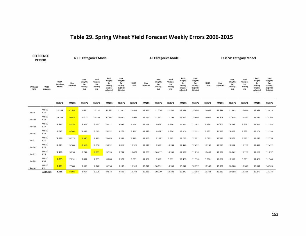
153

Table 29. Spring Wheat Yield Forecast Weekly Errors 2006-2015

REFERENCE PERIOD

G + E Categories Model All Categories Model Less VP Category Model

AVERAGE DATE

WEEK NUMBER

USDA Data Base

Model

Bias Adjusted

Prod Weights

3yr moving

avg

Prod Weights

5yr moving

avg

Prod Weights

3yr moving avg Bias Adjusted

Prod Weights

5yr moving avg Bias Adjusted

USDA Data

Bias Adjusted

Prod Weights

3yr moving

avg

Prod Weights

5yr moving

avg

Prod Weights

3yr moving avg Bias Adjusted

Prod Weights

5yr moving avg Bias Adjusted

USDA Data

Bias Adjusted

Prod Weights

3yr moving

avg

Prod Weights

5yr moving

avg

Prod Weights

3yr moving avg Bias Adjusted

Prod Weights

5yr moving avg Bias Adjusted

RMSPE RMSPE RMSPE RMSPE RMSPE RMSPE RMSPE RMSPE RMSPE RMSPE RMSPE RMSPE RMSPE RMSPE RMSPE RMSPE RMSPE RMSPE

Jun-9 WEEK #23

11.226 10.949 10.991 11.121 11.550 11.441 11.984 13.850 11.776 11.584 13.938 13.406 12.067 13.888 11.843 11.681 13.938 13.415

Jun-16 WEEK #24

10.772 9.845 10.212 10.356 10.417 10.442 11.902 13.762 11.581 11.798 13.717 13.680 12.021 13.808 11.654 11.880 13.717 13.704

Jun-23 WEEK #25

9.242 8.355 8.929 9.171 9.017 9.042 9.678 11.766 9.601 9.674 11.861 11.762 9.534 11.802 9.533 9.616 11.861 11.788

Jun-30 WEEK #26

9.047 8.564 8.865 9.083 9.232 9.276 9.179 11.817 9.424 9.534 12.104 12.122 9.137 11.830 9.402 9.579 12.104 12.134

Jul-7 WEEK #27

8.639 8.723 8.390 8.473 9.405 9.533 9.142 11.865 9.157 9.582 12.019 12.091 9.029 11.879 9.071 9.523 12.019 12.110

Jul-14 WEEK #28

8.521 9.106 8.513 8.606 9.852 9.817 10.327 12.611 9.965 10.244 12.448 12.452 10.242 12.623 9.884 10.226 12.448 12.472

Jul-21 WEEK #29

8.769 9.230 8.744 8.633 9.795 9.734 10.677 12.269 10.417 10.333 12.187 11.818 10.435 12.286 10.262 10.226 12.187 11.837

Jul-28 WEEK #30

7.365 7.851 7.887 7.885 8.800 8.577 9.883 11.358 9.968 9.891 11.406 11.336 9.916 11.362 9.963 9.881 11.406 11.340

Aug-4 WEEK #31

7.281 7.500 7.695 7.740 8.130 8.130 10.313 10.772 10.091 10.353 10.542 10.757 10.347 10.782 10.088 10.305 10.542 10.769

AVERAGE 8.985 8.902 8.914 9.008 9.578 9.555 10.343 12.230 10.220 10.332 12.247 12.158 10.303 12.251 10.189 10.324 12.247 12.174

154

Table 30. Spring Wheat Yield Forecast Weekly Errors 2006-2015 RMSPE RATIO

REFERENCE PERIOD

G + E Categories Model All Categories Model Less VP Category Model

AVERAGE DATE

WEEK NUMBER

USDA Data Base

Model

Bias Adjusted

Prod Weights

3yr moving

avg

Prod Weights

5yr moving

avg

Prod Weights

3yr moving avg Bias Adjusted

Prod Weights

5yr moving avg Bias Adjusted

USDA Data

Bias Adjusted

Prod Weights

3yr moving

avg

Prod Weights

5yr moving

avg

Prod Weights

3yr moving avg Bias Adjusted

Prod Weights

5yr moving avg Bias Adjusted

USDA Data

Bias Adjusted

Prod Weights

3yr moving

avg

Prod Weights

5yr moving

avg

Prod Weights

3yr moving avg Bias Adjusted

Prod Weights

5yr moving avg Bias Adjusted

RMSPE RMSPE RMSPE RMSPE RMSPE RMSPE RMSPE RMSPE RMSPE RMSPE RMSPE RMSPE RMSPE RMSPE RMSPE RMSPE RMSPE RMSPE

Jun-9 WEEK #23

1.000 0.975 0.979 0.991 1.029 1.019 1.067 1.234 1.049 1.032 1.242 1.194 1.075 1.237 1.055 1.041 1.242 1.195

Jun-16 WEEK #24

1.000 0.914 0.948 0.961 0.967 0.969 1.105 1.278 1.075 1.095 1.273 1.270 1.116 1.282 1.082 1.103 1.273 1.272

Jun-23 WEEK #25

1.000 0.904 0.966 0.992 0.976 0.978 1.047 1.273 1.039 1.047 1.283 1.273 1.032 1.277 1.031 1.040 1.283 1.275

Jun-30 WEEK #26

1.000 0.947 0.980 1.004 1.020 1.025 1.015 1.306 1.042 1.054 1.338 1.340 1.010 1.308 1.039 1.059 1.338 1.341

Jul-7 WEEK #27

1.000 1.010 0.971 0.981 1.089 1.104 1.058 1.373 1.060 1.109 1.391 1.400 1.045 1.375 1.050 1.102 1.391 1.402

Jul-14 WEEK #28

1.000 1.069 0.999 1.010 1.156 1.152 1.212 1.480 1.169 1.202 1.461 1.461 1.202 1.481 1.160 1.200 1.461 1.464

Jul-21 WEEK #29

1.000 1.053 0.997 0.985 1.117 1.110 1.218 1.399 1.188 1.178 1.390 1.348 1.190 1.401 1.170 1.166 1.390 1.350

Jul-28 WEEK #30

1.000 1.066 1.071 1.071 1.195 1.165 1.342 1.542 1.353 1.343 1.549 1.539 1.346 1.543 1.353 1.342 1.549 1.540

Aug-4 WEEK #31

1.000 1.030 1.057 1.063 1.117 1.117 1.416 1.479 1.386 1.422 1.448 1.477 1.421 1.481 1.386 1.415 1.448 1.479

AVERAGE 1.000 0.996 0.996 1.006 1.074 1.071 1.164 1.374 1.151 1.165 1.375 1.367 1.160 1.376 1.147 1.163 1.375 1.369

155

Table 31. Corn Yield Forecast Error Comparison 2006-2015

YEAR WASDE Release

Date

WASDE Yield

Best Performing Model Yield

Composite Yield

January Final Yield

WASDE APE (%)

Best Performing Model APE

(%)

Composite APE (%)

YEAR WASDE Release

Date

WASDE Yield

Best Performing Model Yield

Composite Yield

January Final Yield

WASDE APE (%)

Best Performing Model APE

(%)

Composite APE (%)

TREND YIELD MONTHS SURVEY YIELD MONTHS

June August

2006 9-Jun 149.0 153.6 151.3 149.1 0.1 3.0 1.5 2006 11-Aug 152.2 151.6 151.9 149.1 2.1 1.7 1.9

2007 11-Jun 150.3 157.5 153.9 150.7 0.3 4.5 2.4 2007 10-Aug 152.8 150.1 151.5 150.7 1.4 0.4 0.9

2008 10-Jun 148.9 150.6 149.8 153.3 2.9 1.8 2.3 2008 12-Aug 155.0 155.5 155.3 153.3 1.1 1.5 1.3

2009 10-Jun 153.4 157.7 155.6 164.4 6.7 4.1 5.4 2009 12-Aug 159.5 161.6 160.6 164.4 3.0 1.7 2.3

2010 10-Jun 163.5 163.6 163.6 152.6 7.1 7.2 7.2 2010 12-Aug 165.0 165.5 165.3 152.6 8.1 8.5 8.3

2011 9-Jun 158.7 159.3 159.0 146.8 8.1 8.5 8.3 2011 11-Aug 153.0 156.1 154.6 146.8 4.2 6.4 5.3

2012 12-Jun 166.0 158.9 162.4 123.1 34.8 29.1 32.0 2012 10-Aug 123.4 123.4 123.4 123.1 0.2 0.2 0.2

2013 12-Jun 156.5 157.5 157.0 158.1 1.0 0.4 0.7 2013 12-Aug 154.4 163.5 159.0 158.1 2.3 3.4 2.9

2014 11-Jun 165.3 168.6 166.9 171.0 3.3 1.4 2.4 2014 12-Aug 167.4 174.8 171.1 171.0 2.1 2.2 2.2

2015 10-Jun 166.8 169.8 168.3 168.4 1.0 0.9 0.9 2015 12-Aug 168.8 171.9 170.4 168.4 0.2 2.1 1.2

G+E Model

MAPE 6.5 6.1 6.3 Less VP category Model

MAPE 2.5 2.8 2.6

3-yr moving avg bias adjusted

3-yr moving avg

July September

2006 12-Jul 149.0 148.4 148.7 149.1 0.1 0.4 0.3 2006 12-Sep 154.7 153.1 153.9 149.1 3.8 2.7 3.2

2007 12-Jul 150.3 154.2 152.3 150.7 0.3 2.3 1.3 2007 12-Sep 152.8 152.2 152.5 150.7 1.4 1.0 1.2

2008 11-Jul 148.4 144.0 146.2 153.3 3.2 6.1 4.6 2008 12-Sep 152.3 151.3 151.8 153.3 0.7 1.3 1.0

2009 10-Jul 153.4 157.7 155.5 164.4 6.7 4.1 5.4 2009 11-Sep 161.9 162.9 162.4 164.4 1.5 0.9 1.2

2010 9-Jul 163.5 159.0 161.2 152.6 7.1 4.2 5.7 2010 10-Sep 162.5 162.9 162.7 152.6 6.5 6.8 6.6

2011 12-Jul 158.7 158.8 158.8 146.8 8.1 8.2 8.1 2011 12-Sep 148.1 149.2 148.7 146.8 0.9 1.6 1.3

2012 11-Jul 146.0 136.9 141.4 123.1 18.6 11.2 14.9 2012 12-Sep 122.8 124.1 123.5 123.1 0.2 0.8 0.5

2013 11-Jul 156.5 159.0 157.8 158.1 1.0 0.6 0.8 2013 12-Sep 155.3 152.6 154.0 158.1 1.8 3.5 2.6

2014 11-Jul 165.3 169.1 167.2 171.0 3.3 1.1 2.2 2014 11-Sep 171.7 176.1 173.9 171.0 0.4 3.0 1.7

2015 10-Jul 166.8 163.3 165.0 168.4 1.0 3.0 2.0 2015 11-Sep 167.5 171.7 169.6 168.4 0.5 2.0 1.3

All categories Model MAPE 4.9 4.1 4.5 Less VP category Model

MAPE 1.8 2.4 2.1

3-yr moving avg bias adjusted

3-yr moving avg

156

Table 32. Corn Yield Forecast Error Comparison 2006-2015

YEAR WASDE Release

Date

WASDE Yield

Best Performing

Model Yield

Composite Yield

January Final Yield

WASDE SPE (%)

Best Performing Model SPE

(%)

Composite SPE (%)

YEAR WASDE Release

Date

WASDE Yield

Best Performing

Model Yield

Composite Yield

January Final Yield

WASDE SPE (%)

Best Performing Model SPE

(%)

Composite SPE (%)

TREND YIELD MONTHS SURVEY YIELD MONTHS

June August

2006 9-Jun 149.0 158.1 153.6 149.1 0.0 36.7 18.3 2006 11-Aug 152.2 151.6 151.9 149.1 4.3 2.7 3.5

2007 11-Jun 150.3 159.3 154.8 150.7 0.1 32.7 16.4 2007 10-Aug 152.8 150.1 151.5 150.7 1.9 0.1 1.0

2008 10-Jun 148.9 139.8 144.4 153.3 8.2 77.3 42.8 2008 12-Aug 155.0 155.5 155.3 153.3 1.2 2.1 1.7

2009 10-Jun 153.4 155.0 154.2 164.4 44.8 32.9 38.8 2009 12-Aug 159.5 161.6 160.6 164.4 8.9 2.9 5.9

2010 10-Jun 163.5 163.0 163.3 152.6 51.0 46.8 48.9 2010 12-Aug 165.0 165.5 165.3 152.6 66.0 72.0 69.0

2011 9-Jun 158.7 154.7 156.7 146.8 65.7 28.9 47.3 2011 11-Aug 153.0 156.1 154.6 146.8 17.8 40.3 29.1

2012 12-Jun 166.0 150.5 158.3 123.1 1214.5 495.8 855.1 2012 10-Aug 123.4 123.4 123.4 123.1 0.1 0.1 0.1

2013 12-Jun 156.5 152.2 154.3 158.1 1.0 14.1 7.6 2013 12-Aug 154.4 163.5 159.0 158.1 5.5 11.8 8.6

2014 11-Jun 165.3 166.0 165.7 171.0 11.1 8.4 9.8 2014 12-Aug 167.4 174.8 171.1 171.0 4.4 5.0 4.7

2015 10-Jun 166.8 165.6 166.2 168.4 0.9 2.9 1.9 2015 12-Aug 168.8 171.9 170.4 168.4 0.1 4.4 2.2

All categories Model RMSPE 11.8 8.8 10.3 Less VP category Model

RMSPE 3.3 3.8 3.5

3-yr moving avg bias adjusted

3-yr moving avg

July September

2006 12-Jul 149.0 148.4 148.7 149.1 0.0 0.2 0.1 2006 12-Sep 154.7 153.1 153.9 149.1 14.1 7.1 10.6

2007 12-Jul 150.3 154.2 152.3 150.7 0.1 5.4 2.7 2007 12-Sep 152.8 152.2 152.5 150.7 1.9 1.0 1.5

2008 11-Jul 148.4 144.0 146.2 153.3 10.2 37.0 23.6 2008 12-Sep 152.3 151.3 151.8 153.3 0.4 1.8 1.1

2009 10-Jul 153.4 157.7 155.5 164.4 44.8 16.7 30.7 2009 11-Sep 161.9 162.9 162.4 164.4 2.3 0.9 1.6

2010 9-Jul 163.5 159.0 161.2 152.6 51.0 17.5 34.3 2010 10-Sep 162.5 162.9 162.7 152.6 42.1 45.8 44.0

2011 12-Jul 158.7 158.8 158.8 146.8 65.7 67.0 66.4 2011 12-Sep 148.1 149.2 148.7 146.8 0.8 2.7 1.7

2012 11-Jul 146.0 136.9 141.4 123.1 346.1 124.8 235.4 2012 12-Sep 122.8 124.1 123.5 123.1 0.1 0.7 0.4

2013 11-Jul 156.5 159.0 157.8 158.1 1.0 0.4 0.7 2013 12-Sep 155.3 152.6 154.0 158.1 3.1 12.1 7.6

2014 11-Jul 165.3 169.1 167.2 171.0 11.1 1.2 6.2 2014 11-Sep 171.7 176.1 173.9 171.0 0.2 8.9 4.5

2015 10-Jul 166.8 163.3 165.0 168.4 0.9 9.2 5.1 2015 11-Sep 167.5 171.7 169.6 168.4 0.3 3.9 2.1

All categories Model RMSPE 7.3 5.3 6.3 Less VP category Model

RMSPE 2.6 2.9 2.7

3-yr moving avg bias adjusted

3-yr moving avg

157

Table 33.Soybean Yield Forecast Error Comparison 2006-2015

YEAR WASDE Release

Date WASDE Yield

Best Performing Model Yield

Composite Yield January Final Yield WASDE APE (%) Best Performing Model APE (%)

Composite APE (%)

TREND YIELD MONTH

July 2006 12-Jul 40.7 40.8 40.8 42.9 5.1 4.9 5.0 2007 12-Jul 41.5 42.4 42.0 41.7 0.5 1.7 1.1 2008 11-Jul 41.6 42.2 41.9 39.7 4.8 6.4 5.6 2009 10-Jul 42.6 43.4 43.0 44.0 3.2 1.5 2.3 2010 9-Jul 42.9 43.6 43.2 43.5 1.4 0.2 0.8 2011 12-Jul 43.4 43.6 43.5 42.0 3.3 3.9 3.6 2012 11-Jul 40.5 38.9 39.7 40.0 1.3 2.7 2.0 2013 11-Jul 44.5 43.7 44.1 44.0 1.1 0.8 1.0 2014 11-Jul 45.2 46.3 45.8 47.5 4.8 2.5 3.7 2015 10-Jul 46.0 44.6 45.3 48.0 4.2 7.2 5.7

All categories Model MAPE 3.0 3.2 3.1

Bias adjusted SURVEY YIELD MONTHS

August 2006 11-Aug 39.6 40.8 40.2 42.9 7.7 4.9 6.3 2007 10-Aug 41.5 41.7 41.6 41.7 0.5 0.0 0.3 2008 12-Aug 40.5 43.5 42.0 39.7 2.0 9.6 5.8 2009 12-Aug 41.7 43.9 42.8 44.0 5.2 0.3 2.8 2010 12-Aug 44.0 44.7 44.3 43.5 1.1 2.7 1.9 2011 11-Aug 41.4 43.0 42.2 42.0 1.4 2.4 1.9 2012 10-Aug 36.1 38.3 37.2 40.0 9.8 4.2 7.0 2013 12-Aug 42.6 44.0 43.3 44.0 3.2 0.0 1.6 2014 12-Aug 45.4 46.1 45.7 47.5 4.4 3.0 3.7 2015 12-Aug 46.9 45.0 46.0 48.0 2.3 6.2 4.3

All categories Model MAPE 3.8 3.3 3.6

Bias adjusted September

2006 12-Sep 39.6 43.2 41.4 42.9 7.7 0.4 4.1 2007 12-Sep 41.4 42.7 42.0 41.7 0.7 1.3 1.0 2008 12-Sep 40.0 43.0 41.5 39.7 0.8 7.4 4.1 2009 11-Sep 42.3 44.4 43.3 44.0 3.9 0.2 2.0 2010 10-Sep 44.7 44.6 44.7 43.5 2.8 1.4 2.1 2011 12-Sep 41.8 42.4 42.1 42.0 0.5 0.2 0.4 2012 12-Sep 35.3 39.6 37.5 40.0 11.8 2.3 7.0 2013 12-Sep 41.2 42.7 42.0 44.0 6.4 4.2 5.3 2014 11-Sep 46.6 47.3 47.0 47.5 1.9 1.3 1.6 2015 11-Sep 47.1 45.8 46.4 48.0 1.9 5.8 3.8

All categories Model MAPE 3.8 2.5 3.1

USDA original

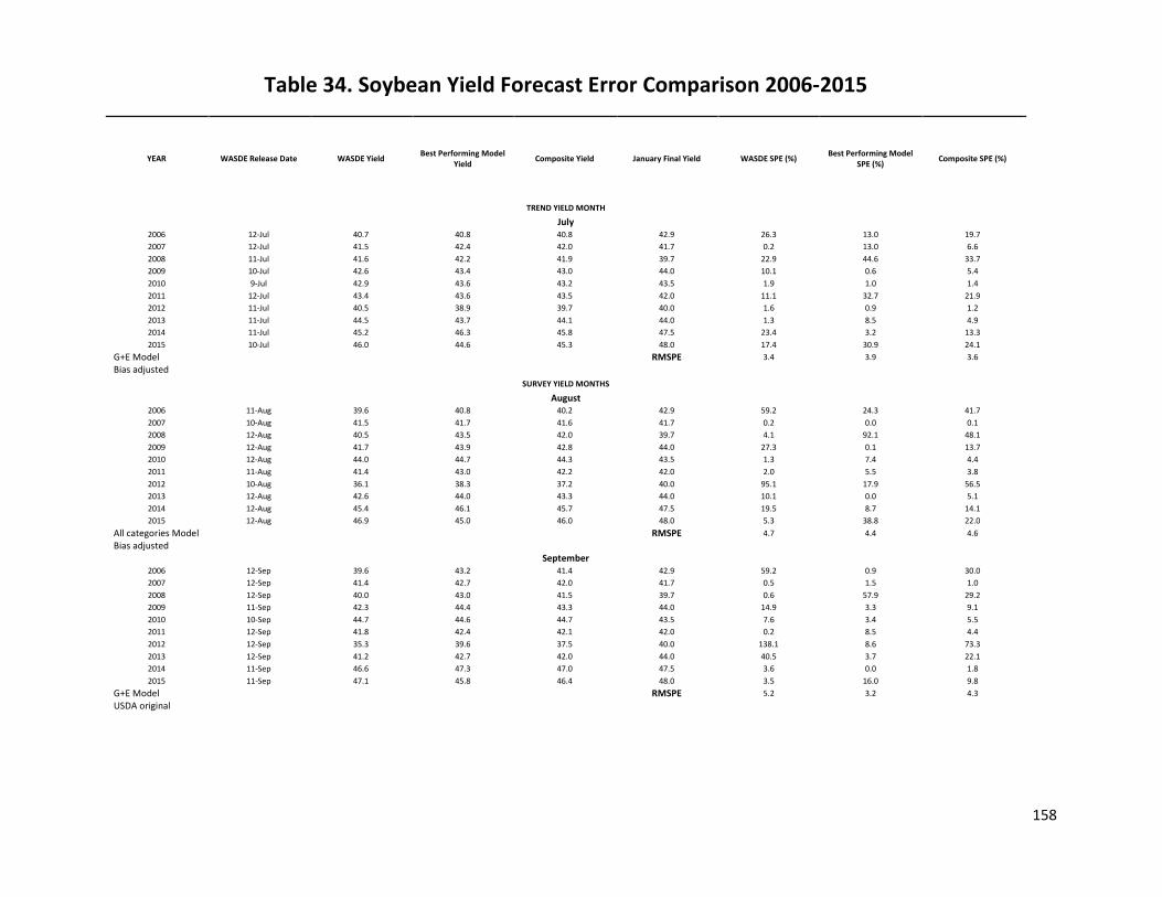
158

Table 34. Soybean Yield Forecast Error Comparison 2006-2015

YEAR WASDE Release Date WASDE Yield Best Performing Model

Yield Composite Yield January Final Yield WASDE SPE (%)

Best Performing Model SPE (%)

Composite SPE (%)

TREND YIELD MONTH

July 2006 12-Jul 40.7 40.8 40.8 42.9 26.3 13.0 19.7

2007 12-Jul 41.5 42.4 42.0 41.7 0.2 13.0 6.6

2008 11-Jul 41.6 42.2 41.9 39.7 22.9 44.6 33.7

2009 10-Jul 42.6 43.4 43.0 44.0 10.1 0.6 5.4

2010 9-Jul 42.9 43.6 43.2 43.5 1.9 1.0 1.4

2011 12-Jul 43.4 43.6 43.5 42.0 11.1 32.7 21.9

2012 11-Jul 40.5 38.9 39.7 40.0 1.6 0.9 1.2

2013 11-Jul 44.5 43.7 44.1 44.0 1.3 8.5 4.9

2014 11-Jul 45.2 46.3 45.8 47.5 23.4 3.2 13.3

2015 10-Jul 46.0 44.6 45.3 48.0 17.4 30.9 24.1

G+E Model RMSPE 3.4 3.9 3.6

Bias adjusted

SURVEY YIELD MONTHS

August 2006 11-Aug 39.6 40.8 40.2 42.9 59.2 24.3 41.7

2007 10-Aug 41.5 41.7 41.6 41.7 0.2 0.0 0.1

2008 12-Aug 40.5 43.5 42.0 39.7 4.1 92.1 48.1

2009 12-Aug 41.7 43.9 42.8 44.0 27.3 0.1 13.7

2010 12-Aug 44.0 44.7 44.3 43.5 1.3 7.4 4.4

2011 11-Aug 41.4 43.0 42.2 42.0 2.0 5.5 3.8

2012 10-Aug 36.1 38.3 37.2 40.0 95.1 17.9 56.5

2013 12-Aug 42.6 44.0 43.3 44.0 10.1 0.0 5.1

2014 12-Aug 45.4 46.1 45.7 47.5 19.5 8.7 14.1

2015 12-Aug 46.9 45.0 46.0 48.0 5.3 38.8 22.0

All categories Model RMSPE 4.7 4.4 4.6

Bias adjusted September

2006 12-Sep 39.6 43.2 41.4 42.9 59.2 0.9 30.0

2007 12-Sep 41.4 42.7 42.0 41.7 0.5 1.5 1.0

2008 12-Sep 40.0 43.0 41.5 39.7 0.6 57.9 29.2

2009 11-Sep 42.3 44.4 43.3 44.0 14.9 3.3 9.1

2010 10-Sep 44.7 44.6 44.7 43.5 7.6 3.4 5.5

2011 12-Sep 41.8 42.4 42.1 42.0 0.2 8.5 4.4

2012 12-Sep 35.3 39.6 37.5 40.0 138.1 8.6 73.3

2013 12-Sep 41.2 42.7 42.0 44.0 40.5 3.7 22.1

2014 11-Sep 46.6 47.3 47.0 47.5 3.6 0.0 1.8

2015 11-Sep 47.1 45.8 46.4 48.0 3.5 16.0 9.8

G+E Model RMSPE 5.2 3.2 4.3

USDA original

159

Table 35. Cotton, Upland Yield Forecast Error Comparison 2006-2015

YEAR WASDE Release Date WASDE Yield Best Performing Model

Yield Composite Yield January Final Yield WASDE APE (%)

Best Performing Model APE (%)

Composite APE (%)

TREND YIELD MONTH

July 2006 12-Jul 770.0 687.2 728.6 806.0 4.5 15.6 10.0

2007 12-Jul 800.0 773.1 786.5 864.0 7.4 12.1 9.7

2008 11-Jul 830.0 793.4 811.7 804.0 3.2 2.4 2.8

2009 10-Jul 805.0 762.0 783.5 765.0 5.2 1.8 3.5

2010 9-Jul 845.0 905.1 875.1 805.0 5.0 11.5 8.2

2011 12-Jul 800.0 783.3 791.6 772.0 3.6 0.9 2.2

2012 11-Jul 785.0 796.0 790.5 874.0 10.2 10.8 10.5

2013 11-Jul 831.0 833.7 832.3 802.0 3.6 1.5 2.6

2014 11-Jul 816.0 883.3 849.7 826.0 1.2 5.4 3.3

2015 10-Jul 819.0 883.7 851.4 755.0 8.5 14.9 11.7

All categories Model MAPE 5.2 7.7 6.5

Bias adjusted

SURVEY YIELD MONTHS

August 2006 11-Aug 751.0 674.8 712.9 806.0 6.8 17.1 12.0

2007 10-Aug 767.0 768.3 767.7 864.0 11.2 12.6 11.9

2008 12-Aug 831.0 763.8 797.4 804.0 3.4 6.0 4.7

2009 12-Aug 809.0 789.8 799.4 765.0 5.8 1.8 3.8

2010 12-Aug 831.0 861.4 846.2 805.0 3.2 6.1 4.7

2011 11-Aug 809.0 726.2 767.6 772.0 4.8 8.1 6.4

2012 10-Aug 771.0 787.1 779.0 874.0 11.8 11.8 11.8

2013 12-Aug 796.0 822.7 809.3 802.0 0.7 0.2 0.5

2014 12-Aug 808.0 860.7 834.4 826.0 2.2 2.7 2.4

2015 12-Aug 784.0 882.5 833.3 755.0 3.8 14.8 9.3

G+E Model MAPE 5.4 8.1 6.7

Bias adjusted September

2006 12-Sep 750.0 690.2 720.1 806.0 6.9 15.2 11.1

2007 12-Sep 797.0 771.1 784.1 864.0 7.8 12.3 10.0

2008 12-Sep 839.0 783.0 811.0 804.0 4.4 3.7 4.0

2009 11-Sep 827.0 804.9 815.9 765.0 8.1 3.7 5.9

2010 10-Sep 833.0 848.0 840.5 805.0 3.5 4.4 4.0

2011 12-Sep 794.0 729.0 761.5 772.0 2.8 7.7 5.3

2012 12-Sep 774.0 797.6 785.8 874.0 11.4 10.6 11.0

2013 12-Sep 777.0 833.2 805.1 802.0 3.1 1.5 2.3

2014 11-Sep 790.0 855.7 822.8 826.0 4.4 2.1 3.2

2015 11-Sep 777.0 877.5 827.3 755.0 2.9 14.1 8.5

G+E Model MAPE 5.5 7.5 6.5

Bias adjusted

160

Table 36. Cotton, Upland Yield Forecast Error Comparison 2006-2015

YEAR WASDE Release Date WASDE Yield Best Performing

Model Yield Composite Yield January Final Yield WASDE SPE (%)

Best Performing Model SPE (%)

Composite SPE (%)

TREND YIELD MONTH

July 2006 12-Jul 770.0 704.7 737.4 806.0 19.9 180.3 100.1 2007 12-Jul 800.0 788.9 794.4 864.0 54.9 105.1 80.0 2008 11-Jul 830.0 772.8 801.4 804.0 10.5 24.5 17.5 2009 10-Jul 805.0 774.3 789.7 765.0 27.3 0.0 13.7 2010 9-Jul 845.0 886.7 865.9 805.0 24.7 84.7 54.7 2011 12-Jul 800.0 735.1 767.5 772.0 13.2 48.3 30.7 2012 11-Jul 785.0 815.2 800.1 874.0 103.7 74.1 88.9 2013 11-Jul 831.0 835.1 833.1 802.0 13.1 3.0 8.0 2014 11-Jul 816.0 884.9 850.4 826.0 1.5 31.3 16.4 2015 10-Jul 819.0 898.7 858.9 755.0 71.9 284.6 178.2

G+E Model RMSPE 5.8 9.1 7.7

USDA original SURVEY YIELD MONTHS

August 2006 11-Aug 751.0 692.2 721.6 806.0 46.6 223.8 135.2 2007 10-Aug 767.0 784.9 776.0 864.0 126.0 114.5 120.3 2008 12-Aug 831.0 780.9 806.0 804.0 11.3 15.5 13.4 2009 12-Aug 809.0 806.9 808.0 765.0 33.1 15.9 24.5 2010 12-Aug 831.0 878.6 854.8 805.0 10.4 67.2 38.8 2011 11-Aug 809.0 743.2 776.1 772.0 23.0 35.2 29.1 2012 10-Aug 771.0 803.5 787.2 874.0 138.9 98.4 118.7 2013 12-Aug 796.0 839.0 817.5 802.0 0.6 4.8 2.7 2014 12-Aug 808.0 877.1 842.5 826.0 4.7 21.8 13.3 2015 12-Aug 784.0 898.7 841.4 755.0 14.8 284.6 149.7

G+E Model RMSPE 6.4 9.4 8.0

USDA original September

2006 12-Sep 750.0 696.4 723.2 806.0 48.3 208.7 128.5 2007 12-Sep 797.0 777.0 787.0 864.0 60.1 134.6 97.3 2008 12-Sep 839.0 789.1 814.1 804.0 19.0 8.6 13.8 2009 11-Sep 827.0 811.0 819.0 765.0 65.7 20.3 43.0 2010 10-Sep 833.0 854.1 843.5 805.0 12.1 26.9 19.5 2011 12-Sep 794.0 735.1 764.5 772.0 8.1 48.3 28.2 2012 12-Sep 774.0 803.5 788.7 874.0 130.9 98.4 114.7 2013 12-Sep 777.0 839.0 808.0 802.0 9.7 4.8 7.3 2014 11-Sep 790.0 861.5 825.8 826.0 19.0 7.9 13.4 2015 11-Sep 777.0 883.3 830.1 755.0 8.5 220.9 114.7

G+E Model RMSPE 6.2 8.8 7.6

USDA original

161

Table 37. Winter Wheat Yield Forecast Error Comparison 2006-2015

YEAR WASDE Release Date WASDE Yield Best Performing

Model Yield Composite Yield January Final Yield WASDE APE (%)

Best Performing Model APE (%)

Composite APE (%)

April 2006 10-Apr 42.0 43.0 42.5 41.6 1.0 3.5 2.2

2007 10-Apr 38.7 45.5 42.1 41.7 7.2 9.1 8.1

2008 9-Apr 40.5 41.7 41.1 47.1 14.0 11.4 12.7

2009 9-Apr 44.9 42.9 43.9 44.0 2.0 2.4 2.2

2010 9-Apr 44.4 47.6 46.0 46.5 4.5 2.3 3.4

2011 8-Apr 46.4 42.2 44.3 46.1 0.7 8.5 4.6

2012 10-Apr 43.7 47.6 45.6 47.1 7.2 1.0 4.1

2013 10-Apr 46.3 44.8 45.5 47.3 2.1 5.3 3.7

2014 9-Apr 47.2 44.0 45.6 42.6 10.8 3.2 7.0

2015 9-Apr 43.7 42.6 43.1 42.5 2.8 0.1 1.5

Less VP category Model MAPE 5.2 4.7 5.0

3-yr moving avg bias adjusted May

2006 12-May 42.4 42.5 42.5 41.6 1.9 2.2 2.1

2007 11-May 43.5 45.7 44.6 41.7 4.3 9.6 7.0

2008 9-May 44.3 43.6 44.0 47.1 5.9 7.4 6.7

2009 12-May 44.2 45.1 44.6 44.0 0.5 2.5 1.5

2010 11-May 45.9 47.8 46.9 46.5 1.3 2.9 2.1

2011 11-May 44.5 42.5 43.5 46.1 3.5 7.8 5.6

2012 10-May 47.6 48.8 48.2 47.1 1.1 3.7 2.4

2013 10-May 45.4 44.2 44.8 47.3 4.0 6.6 5.3

2014 9-May 43.1 43.7 43.4 42.6 1.2 2.6 1.9

2015 12-May 43.5 43.3 43.4 42.5 2.4 2.0 2.2

Less VP category Model MAPE 2.6 4.7 3.7

3-yr moving avg bias adjusted June

2006 9-Jun 40.5 41.4 40.9 41.6 2.6 0.6 1.6

2007 11-Jun 43.2 46.4 44.8 41.7 3.6 11.2 7.4

2008 10-Jun 45.3 45.4 45.3 47.1 3.8 3.7 3.8

2009 10-Jun 43.9 45.7 44.8 44.0 0.2 4.0 2.1

2010 10-Jun 46.6 49.1 47.8 46.5 0.2 5.5 2.9

2011 9-Jun 45.3 44.5 44.9 46.1 1.7 3.4 2.6

2012 12-Jun 47.3 47.5 47.4 47.1 0.4 0.8 0.6

2013 12-Jun 46.1 44.7 45.4 47.3 2.5 5.5 4.0

2014 11-Jun 42.4 45.3 43.8 42.6 0.5 6.3 3.4

2015 10-Jun 44.5 45.3 44.9 42.5 4.7 6.6 5.6

Less VP category Model MAPE 2.0 4.7 3.4

3-yr moving avg bias adjusted

162

Table 38. Winter Wheat Yield Forecast Error Comparison 2006-2015

YEAR WASDE Release Date WASDE Yield Best Performing

Model Yield Composite Yield January Final Yield WASDE SPE (%)

Best Performing Model SPE (%)

Composite SPE (%)

April

2006 10-Apr 42 40.8 41.4 41.6 0.9 3.7 2.3

2007 10-Apr 38.7 45.8 42.2 41.7 51.8 96.0 73.9

2008 9-Apr 40.5 43.7 42.1 47.1 196.4 53.2 124.8

2009 9-Apr 44.9 40.9 42.9 44.0 4.2 49.4 26.8

2010 9-Apr 44.4 48.2 46.3 46.5 20.4 13.8 17.1

2011 8-Apr 46.4 43.8 45.1 46.1 0.4 25.3 12.9

2012 10-Apr 43.7 47.4 45.5 47.1 52.1 0.4 26.2

2013 10-Apr 46.3 44.0 45.1 47.3 4.5 50.1 27.3

2014 9-Apr 47.2 42.7 44.9 42.6 116.6 0.0 58.3

2015 9-Apr 43.7 44.7 44.2 42.5 8.0 27.0 17.5

All categories Model RMSPE 6.7 5.6 38.7

Bias adjusted

May

2006 12-May 42.4 42.2 42.3 41.6 3.7 2.3 3.0

2007 11-May 43.5 45.3 44.4 41.7 18.6 73.8 46.2

2008 9-May 44.3 44.5 44.4 47.1 35.3 29.5 32.4

2009 12-May 44.2 43.1 43.7 44.0 0.2 4.1 2.2

2010 11-May 45.9 48.5 47.2 46.5 1.7 17.8 9.7

2011 11-May 44.5 43.0 43.8 46.1 12.0 44.8 28.4

2012 10-May 47.6 48.5 48.1 47.1 1.1 9.2 5.2

2013 10-May 45.4 43.6 44.5 47.3 16.1 61.7 38.9

2014 9-May 43.1 44.9 44.0 42.6 1.4 29.7 15.6

2015 12-May 43.5 43.5 43.5 42.5 5.5 5.7 5.6

All categories Model RMSPE 3.1 5.3 4.3

5-yr moving avg bias adjusted

June

2006 9-Jun 40.5 41.4 40.9 41.6 7.0 0.3 3.7

2007 11-Jun 43.2 46.4 44.8 41.7 12.9 125.7 69.3

2008 10-Jun 45.3 45.4 45.3 47.1 14.6 13.7 14.1

2009 10-Jun 43.9 45.7 44.8 44.0 0.1 15.8 7.9

2010 10-Jun 46.6 49.1 47.8 46.5 0.0 30.1 15.1

2011 9-Jun 45.3 44.5 44.9 46.1 3.0 11.5 7.3

2012 12-Jun 47.3 47.5 47.4 47.1 0.2 0.6 0.4

2013 12-Jun 46.1 44.7 45.4 47.3 6.4 30.5 18.5

2014 11-Jun 42.4 45.3 43.8 42.6 0.2 39.8 20.0

2015 10-Jun 44.5 45.3 44.9 42.5 22.1 43.2 32.6

Less VP category Model RMSPE 2.6 5.6 18.9

3-yr moving avg bias adjusted

163

Table 39. Spring Wheat Yield Forecast Error Comparison 2006-2015

YEAR WASDE Release Date WASDE Yield Best Performing Model Yield Composite Yield January Final Yield WASDE APE (%) Best Performing Model APE

(%) Composite APE (%)

June

2006 9-Jun 39.3 40.7 40.0 33.2 18.4 22.5 20.4

2007 11-Jun 41.5 44.6 43.0 37.1 11.9 20.2 16.0

2008 10-Jun 43.2 39.7 41.5 40.5 6.7 1.9 4.3

2009 10-Jun 41.2 42.8 42.0 45.2 8.8 5.2 7.0

2010 10-Jun 43.9 46.7 45.3 46.1 4.8 1.4 3.1

2011 9-Jun 43.1 42.7 42.9 37.7 14.3 13.4 13.8

2012 12-Jun 45.4 44.3 44.8 44.9 1.1 1.4 1.3

2013 12-Jun 44.6 42.0 43.3 47.1 5.3 10.9 8.1

2014 11-Jun 42.3 45.0 43.6 46.7 9.4 3.7 6.6

2015 10-Jun 44.2 45.4 44.8 46.3 4.5 1.9 3.2

G+E Model MAPE 8.5 8.2 8.4

USDA original

July

2006 12-Jul 32.9 34.4 33.6 33.2 0.9 3.6 2.2

2007 12-Jul 39.1 43.8 41.5 37.1 5.4 18.2 11.8

2008 11-Jul 36.8 41.1 39.0 40.5 9.1 1.6 5.4

2009 10-Jul 38.3 42.6 40.4 45.2 15.3 5.8 10.5

2010 9-Jul 44.6 46.0 45.3 46.1 3.3 0.2 1.7

2011 12-Jul 41.7 44.0 42.8 37.7 10.6 16.6 13.6

2012 11-Jul 40.4 42.1 41.2 44.9 10.0 6.3 8.2

2013 11-Jul 42.9 44.4 43.7 47.1 8.9 5.7 7.3

2014 11-Jul 45.5 44.7 45.1 46.7 2.6 4.2 3.4

2015 10-Jul 46.7 45.7 46.2 46.3 0.9 1.4 1.1

G+E Model MAPE 6.7 6.3 6.5

USDA original

August

2006 11-Aug 32.7 31.9 32.3 33.2 1.5 4.0 2.7

2007 10-Aug 39.3 41.6 40.5 37.1 5.9 12.2 9.1

2008 12-Aug 36.4 38.1 37.2 40.5 10.1 6.0 8.1

2009 12-Aug 41.5 42.4 41.9 45.2 8.2 6.3 7.2

2010 12-Aug 46.6 45.8 46.2 46.1 1.1 0.7 0.9

2011 11-Aug 42.5 42.2 42.4 37.7 12.7 12.1 12.4

2012 10-Aug 42.8 41.3 42.1 44.9 4.7 8.0 6.3

2013 12-Aug 42.8 43.4 43.1 47.1 9.1 7.8 8.4

2014 12-Aug 46.1 44.7 45.4 46.7 1.3 4.2 2.8

2015 12-Aug 47.0 45.7 46.3 46.3 1.5 1.4 1.4

G+E Model MAPE 5.6 6.3 5.9

USDA original

164

Table 40. Spring Wheat Yield Forecast Error Comparison 2006-2015

YEAR WASDE Release Date WASDE Yield Best Performing Model

Yield Composite Yield January Final Yield WASDE SPE (%)

Best Performing Model SPE (%)

Composite SPE (%)

June

2006 9-Jun 39.3 37.1 38.2 33.2 337.6 140.3 238.9

2007 11-Jun 41.5 41.1 41.3 37.1 140.7 117.5 129.1

2008 10-Jun 43.2 36.4 39.8 40.5 44.4 103.7 74.1

2009 10-Jun 41.2 39.5 40.3 45.2 78.3 159.4 118.9

2010 10-Jun 43.9 43.3 43.6 46.1 22.8 36.5 29.6

2011 9-Jun 43.1 39.3 41.2 37.7 205.2 17.9 111.5

2012 12-Jun 45.4 40.8 43.1 44.9 1.2 82.7 42.0

2013 12-Jun 44.6 38.5 41.6 47.1 28.2 330.2 179.2

2014 11-Jun 42.3 41.5 41.9 46.7 88.8 124.2 106.5

2015 10-Jun 44.2 42.0 43.1 46.3 20.6 86.4 53.5

G+E Model MAPE 9.8 10.9 108.3

3-yr moving avg bias adjusted

July

2006 12-Jul 32.9 33.8 33.3 33.2 0.8 2.8 1.8

2007 12-Jul 39.1 43.0 41.1 37.1 29.1 257.2 143.1

2008 11-Jul 36.8 40.9 38.9 40.5 83.5 1.2 42.3

2009 10-Jul 38.3 42.2 40.2 45.2 233.0 44.5 138.8

2010 9-Jul 44.6 45.9 45.2 46.1 10.6 0.2 5.4

2011 12-Jul 41.7 43.5 42.6 37.7 112.6 238.6 175.6

2012 11-Jul 40.4 41.3 40.9 44.9 100.4 63.3 81.9

2013 11-Jul 42.9 43.5 43.2 47.1 79.5 57.4 68.4

2014 11-Jul 45.5 44.0 44.7 46.7 6.6 34.4 20.5

2015 10-Jul 46.7 45.3 46.0 46.3 0.7 4.3 2.5

G+E Model RMSPE 8.1 8.4 8.2

3-yr moving avg

August

2006 11-Aug 32.7 31.9 32.3 33.2 2.3 15.8 9.1

2007 10-Aug 39.3 41.6 40.5 37.1 35.2 149.0 92.1

2008 12-Aug 36.4 38.1 37.2 40.5 102.5 36.4 69.4

2009 12-Aug 41.5 42.4 41.9 45.2 67.0 39.5 53.2

2010 12-Aug 46.6 45.8 46.2 46.1 1.2 0.5 0.8

2011 11-Aug 42.5 42.2 42.4 37.7 162.1 145.5 153.8

2012 10-Aug 42.8 41.3 42.1 44.9 21.9 63.4 42.6

2013 12-Aug 42.8 43.4 43.1 47.1 83.3 60.3 71.8

2014 12-Aug 46.1 44.7 45.4 46.7 1.7 17.9 9.8

2015 12-Aug 47.0 45.7 46.3 46.3 2.3 1.8 2.1

G+E Model RMSPE 6.9 7.3 7.1

USDA original

165

REFERENCES

Basso, Bruno, Davide Cammarano, and Elisabetta Carfagna. "Review of crop yield forecasting

methods and early warning systems." In Report Presented to First Meeting of the

Scientific Advisory Committee of the Gloal Strategy to Improve Agricultural and Rural

Statistics. FAO, Headquarters, Rome, Italy, pp. 18-19. 2013.

Bouman, B. A. M. "Crop modelling and remote sensing for yield prediction."NJAS journal of life

sciences 43, no. 2 (1995): 143-161.

Doraiswamy, Paul C., Sophie Moulin, Paul W. Cook, and Alan Stern. "Crop yield assessment

from remote sensing." Photogrammetric Engineering & Remote Sensing 69, no. 6 (2003):

665-674.

Fang, Hongliang, Shunlin Liang, Gerrit Hoogenboom, John Teasdale, and Michel Cavigelli.

"Corn‐yield estimation through assimilation of remotely sensed data into the CSM‐

CERES‐Maize model." International Journal of Remote Sensing 29, no. 10 (2008): 3011-

3032.

Fang, Hongliang, Shunlin Liang, and Gerrit Hoogenboom. "Integration of MODIS LAI and

vegetation index products with the CSM–CERES–Maize model for corn yield

estimation." International Journal of Remote Sensing 32, no. 4 (2011): 1039-1065.

Fackler, Paul L., and Bailey Norwood. "Forecasting Crop Yields and Condition Indices."

In NCR-134 Conference on Applied Commodity Price Analysis, Forecasting, and Market

Risk Management, pp. 1-18. 1999.

166

Hodges, T., D. Botner, C. Sakamoto, and J. Hays Haug. "Using the CERES-Maize model to

estimate production for the US Cornbelt." Agricultural and Forest Meteorology 40, no. 4

(1987): 293-303.

Jagtap, Shrikant S., and James W. Jones. "Adaptation and evaluation of the CROPGRO-soybean

model to predict regional yield and production."Agriculture, ecosystems &

environment 93, no. 1 (2002): 73-85.

Johnson, David M. "An assessment of pre-and within-season remotely sensed variables for

forecasting corn and soybean yields in the United States." Remote Sensing of

Environment 141 (2014): 116-128.

Kogan, Felix, Luis Salazar, and Leonid Roytman. "Forecasting crop production using satellite-

based vegetation health indices in Kansas, USA."International journal of remote

sensing 33, no. 9 (2012): 2798-2814.

Kruse, John Robert, and Darnell B. Smith. “Yield estimation throughout the growing season.”

Center for Agricultural and Rural Development, Iowa State University, 1994.

Lehecka, Georg V. "The Reaction of Corn and Soybean Futures Markets to USDA Crop

Progress and Condition Information." In Southern Agricultural Economics Association

Annual (SAEA) Meeting, Orlando, FL. 2013.

Lillesand, Thomas M., and Ralph W. Kiefer. "Remote Sensing and Image Interpretation. John

Willey & Sons." Inc, United States of America (1994).

Matis, J. H., T. Saito, W. E. Grant, W. C. Iwig, and J. T. Ritchie. "A Markov chain approach to

crop yield forecasting." Agricultural systems 18, no. 3 (1985): 171-187.

167

Matis, J. H., T. Birkett, and D. Boudreaux. "An application of the Markov chain approach to

forecasting cotton yields from surveys." Agricultural Systems 29, no. 4 (1989): 357-370.

Moen, Thomas N., Harry M. Kaiser, and Susan J. Riha. "Regional yield estimation using a crop

simulation model: Concepts, methods, and validation." Agricultural Systems 46, no. 1

(1994): 79-92.

Schlenker, Wolfram, and Michael J. Roberts. "Nonlinear temperature effects indicate severe

damages to US crop yields under climate change."Proceedings of the National Academy

of sciences 106, no. 37 (2009): 15594-15598.

Smith, J. Warren. "The effect of weather upon the yield of corn." Monthly Weather Review 42,

no. 2 (1914): 78-92.

Supit, I. "Predicting national wheat yields using a crop simulation and trend

models." Agricultural and Forest Meteorology 88, no. 1 (1997): 199-214.

Tannura, Michael A., Scott H. Irwin, and Darrel L. Good. "Weather, technology, and corn and

soybean yields in the US corn belt." Technology, and Corn and Soybean Yields in the US

Corn Belt (February 1, 2008) (2008).

Thompson, Louis M. "Effects of changes in climate and weather variability on the yields of corn

and soybeans." Journal of Production Agriculture 1, no. 1 (1988): 20-27.

Tucker, Compton J., John RG Townshend, and Thomas E. Goff. "African land-cover

classification using satellite data." Science 227, no. 4685 (1985): 369-375.

Yang, Di. “A spatial analysis of corn and soybean yields and weather relations”. University of

Illinois at Urbana-Champaign. (2011).

168

Wiegand, C. L., A. J. Richardson, and E. T. Kanemasu. "Leaf area index estimates for wheat

from Landsat and their implications for evapotranspiration and crop

modeling." Agronomy Journal 71, no. 2 (1979): 336-342.