Forecasting the Acreage, Yield,

and Price o f Cotton

F. iFHARPER

ttBRAUY, UiMVtRSfr* OF MAKVUM)

A D is s e r t a t io n P r e s e n t e d to t h e G r a d u a t e S c h o o l o f t h k

U n iv e r s it y o f M a r y l a n d i n P a r t ia l F u l f i l l m e n t o f t h e

R e q u ir e m e n t s f o r t h e D e g r e e o f D o c t o r o f P h il o s o p h y

1928

UMI Number: DP70111

Alt rights reserved

INFORMATION TO ALL USERS The quality of this reproduction is dependent upon the quality of the copy submitted.

In the unlikely event that the author did not send a complete manuscript and there are missing pages, these will be noted. Also, if material had to be removed,

a note will indicate the deletion.

UMI'Dissertation Publishing

UMI DP70111

Published by ProQuest LLC (2015). Copyright in the Dissertation held by the Author.

Microform Edition © ProQuest LLC.All rights reserved. This work is protected against

unauthorized copying under Title 17, United States Code

ProQuestProQuest LLC.

789 East Eisenhower Parkway P.O. Box 1346

Ann Arbor, Ml 48106 - 1346

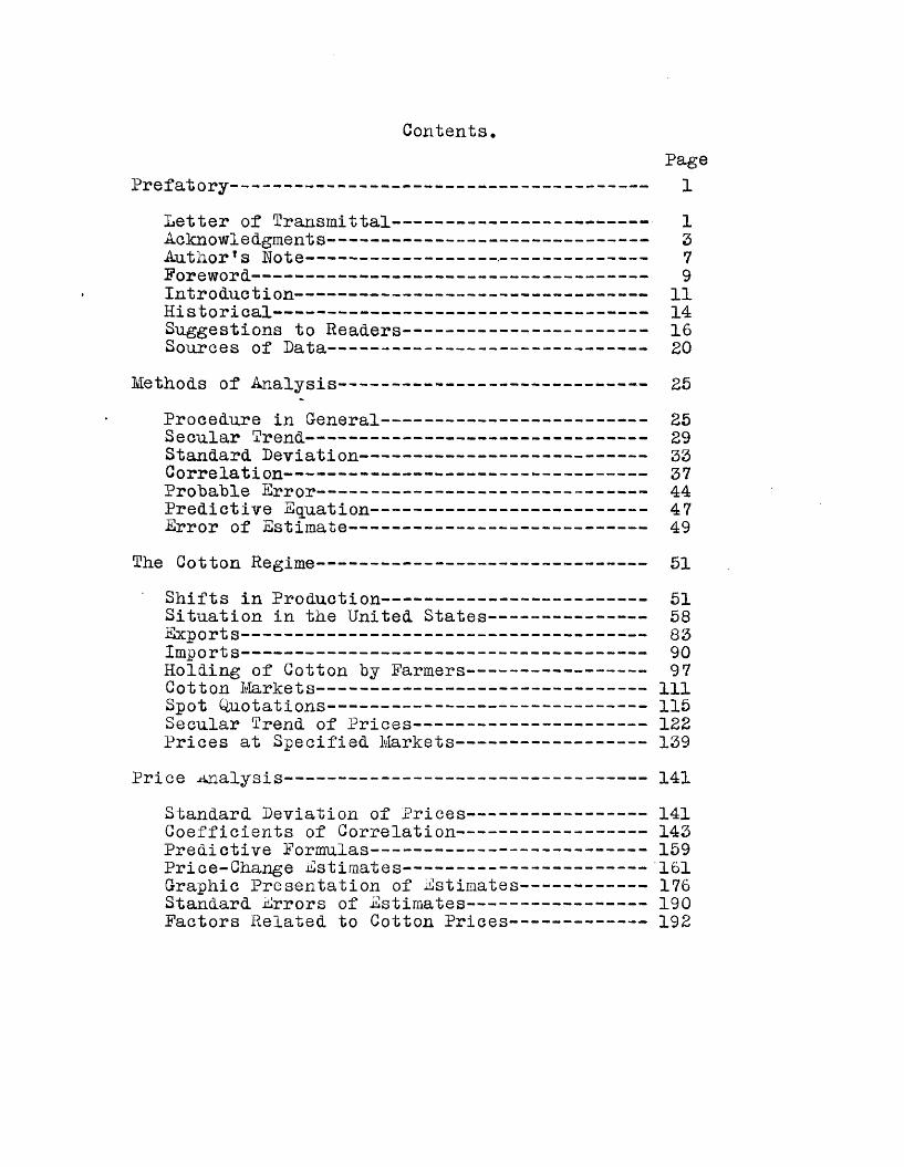
ContentsPage

Prefatory--------------------------------------- 1Letter of Transmittal------------------------ 1Acknowledgments------------------------------ 3AutnorTs Mote------------------.-------------- 7Foreword -------------------------------- 9Introduction--------------------------------- 11Historical----------------------------------- 14Suggestions to Readers----------------------- 16Sources of Data------------------------------ 20

Methods of Analysis----------------------------- 25Procedure in General------------------------- 25Secular Trend-------------------------------- 29Standard Deviation--------------------------- 33Correlation---------------------------------- 37Probable Error------------------------------- 44Predictive Equation-------------------------- 47Error of Estimate---------------------------- 49

The Cotton Regime------------------------------- 51Shifts in Production------------------------- 51Situation in the United States--------------- 58Exports---------------------------------- 83Imports-------------------------------------- 90Holding of Cotton by Farmers----------------- 9 7Cotton Markets-------------------------------- 111Spot Quotations-------------------------------115Secular Trend of Prices-----------------------122Prices at Specified Markets------ 139

Price analysis----------------------------------- 141Standard Deviation of Prices------------------141Coefficients of Correlation-------------------143Predictive Formulas---------------------------159Price-Change Estimates------------------------161Graphic Presentation of Estimates-------------176Standard Errors of Estimates------------------190Factors Related to Cotton Prices--------------192

PageAcreage Analysis-------------------------------- 198

Acreage Harvested---------------------------- 198Acreage Value-------------------------------- 200Undeflated Average Prices--------------------208Farm Products Index Numbers------------------212Deflated Average Prices---------------------- 215Coefficients of Correlation------------------221Acreage Estimates---------------------------- 228

Production Analysis------------:-----------------235Yields per Acre------------------------------ 235Weather Factors------------------------------ 238Measures of Correlation----------------------242Planting Dates------------------------------- 265Monthly Harvestings-------------------------- 267Ratio Estimates------------------------------ 269Par Estimates-------------------------------- 275Recapitulation------------------------------- 283

Conclusions------------------------------------ 285Literature Cited------------------------------- 287

I

Letter of Transmittal

College Park, Maryland,May 15th, 1928.

To the Lean of the Graduate School and the Head of the Department of Agricultural Economics of the University of Maryland.

Sirs: There is transmitted Herewith a report on theforecasting of the acreage, yield, and price of cotton in the United States, giving in a skeletonized form, yet, in sufficient detail to permit an immediate understanding of the problem, the results of four years1 study and research. This work was commenced at the North Carolina State College of Agriculture, was carried on for one year in Washington, and has been completed at the University of Maryland.

The first part of the report deals with spot cotton prices, the factors upon which their fluctuations are de­pendent, and the extent to which they can be predicted on the basis of current cotton production. An analysis has been made of the causal relationship existing between cotton production and subsequent monthly prices, and the degree of this relationship is expressed as coefficients of correlation. Predictive equations are formulated from

2

these expressions of correlation.The second part of the report embodies an analysis

of the extent to which acreage of cotton planted is in­fluenced hy monthly spot prices of cotton produced during the preceding year. Coefficients of correlation have been . calculated from both deflated and undeflated prices, and the predictive equation is formulated in the same way as the equations for price predictions.

The third part of the report deals with the reliability of the par method of production estimate and with the yield of cotton as influenced by various weather factors. Relation­ship between weather factors and subsequent yields is ex­pressed in the same way as the relationship between pro­duction and prices, and prices and subsequent acreage. In addition, the degree of accuracy of par estimates of pro­duction as related to actual production is expressed in terms of correlation coefficients. There is presented also a newly evolved procedure of production estimates, desig­nated as the ratio method.

I cordially transmit to you this report.F.H.Harper

7>

Ackno wl e dgment s

So many have contributed information and assistance of one hind or another in the preparation of this report that I am unable to make mention of all who have aided me, but I hope they will understand that my thoughts are none-the-less sincere because of my failure to mention their names* In a few cases, however, the extent and special character of the service rendered make it quite necessary and proper that I should express publicly my obligation and indebtedness to those who have rendered these services*

If the writer has been successful in finding what he searched for, it has been largely due to the ready good-will and helpful cooperation of many specialists, most of them men whose time is much occupied, but whose interest in this work has led them willingly to place some of it at the writerTs service, and to contribute freely of their knowledge to the perfection of this study*

I wish to acknowledge with grateful appreciation tne suggestion from hr. G. W. Forster, Head of the Depart­ment of Agricultural Economics at the Uorth Carolina State College, that there is a place for such a report

4

on cotton forecasting. It was he who first gave me assistance, and under whose direction the preliminary analysis was made. I desire to express particular thanks to him for his cooperation in the correlation studies of prices. He was of much service in advancing the general economic principles of forecasting, and the value of his suggestions regarding analytical technic is inesti­mable.

Further acknowledgments are due those two gentlemen of the University of Maryland., Hr. S. H. DeVault, Head of the Hepartment of Agricultural Economics, and Professor W. B. Kemp, Assistant Hean of the College of Agriculture, who, not occasionally, but systematically and continuously, have advised with me to improve the work as a whole by criticism, or to enrich it by additions.

Hr. BeVault has spared no effort to perfect his many contributions on the purely economic phases of the problem, and in many instances his aid has been given under con­ditions which necessitated sacrifices of time on his part. He has diligently read and reviewed the proofs from the commencement of tne work and improved them in a systematic way by valuable additions. Many sections owe much of their accuracy and completeness to his assiduous care, and his

5

criticisims and suggestions in regard to the economic aspects of the various phases of forecasting nave enabled me to piirsue my work without interruption.

Professor Kemp has devoted much of his time to a critical examination of the analysis, and his kindly criticism of statistical technic, together with his assistance in the more advanced concepts of correlation, have been a continuous and stimulating source of encourage­ment to me. Without them this study would have been carried forward less rapidly, and much of it would not have reached its final stages. Those who are familiar with Professor KempTs work in correlation, and his numerous findings in other phases of statistics, know with what an amazing wealth of evidence he illustrates the subject upon which he touches. His extensive knowledge has been generously placed at the writer’s service throughout the course of this study, and there is scarcely a principle in corre­lation in my work to Yfhich he has not added a part. It is impossible for me to estimate the value of his assistance in the multiple correlation studies, to the accuracy and completeness of which he has made many additions. He has contributed similarly to the correctness of the ratio-method of estimate, and has revised and corrected the more diffi­cult mathematical equations that have been submitted to

him* Professor Kemp has been generous with his help on all phases requiring further investigation* and, by his personal interest in the field of statistics, has saved the writer many hours of work. The solution of some of the problems confronted seemed at times to be beyond my skill, but the suggestions which came from him encouraged me to renew my efforts in the task before me. I owe him an everlasting debt of gratitude.

The author gratefully acknowledges further the assistance received from Dr. G. F. Cadisch, Assistant lean of the College of Arts and Sciences, University of Maryland. He has read certain sections of my report, and his criticisms have materially aided

me in solving and substantiating various theoretical economic

concepts. Those who know Dr. Cadisch are aware and appreciative

of his marked ability, both as an economic theorist and as a

practical economist. It is this ability, this exceptional power as a critic, that has been so generously placed at my service. I owe him a debt of gratitude which only feelings, not words, can express.

Acknowledgments are due also to members of the cotton trade throughout the country, especially the cotton merchants over the entire South, and the Secretary of the Hew Orleans Cotton Exchange. The author is indebted also to Dr. F. A. Pearson, Professor of Agricultural Economics at Cornell University, and to the corps of workers in the Cotton Division of the United States Department of Agriculture. Of the assistance received from the latter, that of Miss Elna Anderson of the Bureau of Agricultural Economics was outstanding.

7

AuthorTs Note

To the student of economies present themselves these questions: What has been? What tends to be? What causes?The first necessitates historical economic study: the second involves theoretical statistical analysis: the third demands actual interpretation. In the analysis of causal economic relationships, historical tendencies as sources of aid cannot be dispensed with. It is upon these tendencies, these influencing causes and resultant factors, that we make our estimates of probable future conditions. The first two questions, in a way, are tributary to the third. Every­thing is interpreted in terms of past occurrences or ten­dencies, and in order to predict with any appreciable degree of accuracy what will happen in the future we must first know what has contributed to resultant effects of the past. Once the causal factors are known, the next step is to measure their relative influences upon the resultants.

It is the function of economic statistics to assemble, arrange, and analyze economic facts, and to make practical application of the knowledge gained by study and experience, in estimating what are most likely to be the immediate and ultimate effects of various groups of causes. Economic laws, therefore, are statements of tendencies expressed

8

as the most probable occurrences and recurrences, They contribute, along with sound reasoning, a part of the basic material used in solving practical problems.

Historical analysis always involves varying conceptions of the time element, and there is no distinct line of divi­sion between those tendencies which are normal in behavior, abnormal, and occasional. The latter are those in which certain momentary factors exert a pronounced influence, while the former are those resulting in conditions ultimately attained if the economic factors under consideration have sufficient time to work out their full effect undisturbed. Abnormal tendencies are those which the economic factors under question do not allow sufficient time in which to work out their full effect. These tendencies shade into one another by continuous gradations, and those variations which may be regarded as normal if we are thinking of changes from day to day on a cotton exchange are but occasional variations in regard to the tendencies over the period of a year, and these in turn are occasional with reference to tendencies over a quarter of a century. The time element itself is continuous, and it is the factor of greatest difficulty in almost all economic problems. It has no absolute partitions into long and short periods, and what is a long period for one problem is a short period for another.

9

Foreword

Some economic phenomena can be subjected to accurate quantitative measurement* It is hardly conceivable that eco­nomic science could possibly have made much progress had there not been developed certain definite units of quanti­tative expression* When we wish to know the exact distance between points, we do not ask for speculation; we take a yardstick and measure it* If a patient is stricken with disease, the physician does not seek mere opinion, he makes an actual diagnosis. In the field of economics, however, though the need for units and applications of measurements in a quantitative sense is as great as in medicine, we have been guided in the past largely by guesses and opinions. The farmer plants his crop, cultivates it, and, with the forces of nature aiding him, brings it to maturity without giving any thought to potential demand for his product in relation to other products* Collectively, at least, the producers of agricultural commodities have failed to adjust their pro­duction in accordance with general economic principles. Their plantings fluctuate with prices, and they are not based upon the future economic aspects of market demand.

Agriculture has lagged behind industry for a number of years. The■ underlying causes of this are to be found in the fact that agriculture, being less centralized and less in­

10

tensive, has been slower in taking advantage of those greater external economies* Farmers as a group are not lacking in internal economic efficiency, hut rather in those broader economic spheres of orderly production, marketing, and others dependent upon the development of the industry as a whole.

11

Introduetion

Some of the most important problems in economics deal with the inter-relationship between production, prices, and acreage of agricultural products. This inter-relationship is being more fully recognized as time goes on by both pro­duction and marketing specialists, and in some cases it is obvious that marketing organizations handling only a small part of total volume of a particular commodity have suffered losses, and even total failure, because of their attempts to procure higher prices later in the season or during the next crop year. The specialists in economics and marketing are beginning to comprehend the primary causes of abnormally low prices, but the progress of market investigation is making more evident each year the conclusion that in prac­tically all cases the wide fluctuations in prices from year to year are conditioned upon a lack of orderly production. Hbcplanation of the occurrence and extent of relatively low prices, therefore, requires not only the recognition of the causal factor, but also a detailed and comprehensive statis­tical analysis. In the case of most products the first has been easier than the second, since detecting a causal factor is simpler than the analysis of causal conditions. For this reason, we have much more nearly exact knowledge concerning the former. In fact, practically all of our exact data in

12

agricultural economics deal with the causal factor, "but such ideas as are sometimes held concerning the extent to which prices fluctuate in accordance with fluctuations in the causal factor are general and vague, chiefly hased on observation rather than on actual analysis.

The importance of a clearer understanding of the in­fluence of production on prices becomes the more evident when we realize that prices themselves are influencing factors upon acreage of crops planted, and that prices at various times in the year affect quite differently the in­tentions to plant. It is to be expected, of course, that varying sizes of the crop harvested will react in many ways upon the probable crop of the following year as measured on the basis of preceding prices, which, as has been stated, are directly related to acreage planted. Convincing evidence of the causal inter-relationships existing between production, prices, and acreage of cotton will be found in the analysis following.

Experience in marketing problems leads one to believe that price changes can only be understood through exact

(1) It is not, of course, to be inferred that economists have.failed to recognize the importance of supply as related to prices and subsequent extent of planting. Even the earlier economists were aware of the relationship between supply and demand. They realized also the significance of the law of diminishing returns and the fact that market price cannot long remain below the cost of production.

13

analysis of their relations to conditioning factors, and cumulative evidence indicates this to "be particularly true of cotton. The experience of southern farmers in 1926 presents further argument for prompt and critical attention to the relation of production to prices. With cotton selling at six and eight cents a pound it seems evident that recurring depressions can be prevented only through a comprehensive understanding of the price regime. Perhaps at some future time the production and marketing of agricultural products will he controled in much the same way as manufactured commodities.

It is, of course, obvious that there must be some com­prehensive production program if agriculture is to maintain a proper balance over short periods of time. For long periods the tendencies have sufficient time in which to fully manifest themselves, and from this viewpoint there can scarcely be any problem of over-production. It is the seasonal and short time over-production which most seriously affects the producer, and it is because of the disastrous results that agriculture should be placed on a basis that is sound for all periods. It is recognized that the forces of nature are somewhat beyond the control of man, but is it not possible for producers to so organize that the relation between quantities of the various products and the demand for each of them will be more in accord with relative consumption?

Os

14

HistoricalIn the statistical analysis of causal inter-relationships

existing between production, price, and acreage of cotton the studies have been carried on exclusively in the United States.A thorough review of statistical literature shows that four publications, the work of two specialists, have been issued on the subject, and these constitute the total systematic work that has been done.

H. L. Moore (1) found a simple coefficient of correlation of minus .819 between cotton production in the United States and yearly spot prices. Ihen purchasing power of money was taken into consideration as one of the independent variables the multiple coefficient was .859, and in holding the purchasing power of money constant he was able to obtain a coefficient of minus .808. He found that even though there is a coefficient of correlation of plus .492 between cotton prices and general purchasing power, no increased degree of accuracy is to be ob­tained by taking price level into account, neither by incorp­orating its effect in the predictive formula, nor by holding its effect constant by partial correlation.

Between accumulated effects of May rainfall, June temper­ature, and August temperature and the subsequent yield of cotton per acre in Georgia he found a multiple correlation of .732. Similar relationships were calculated for the states of fexas,

15Alabama, and South Carolina, and in most cases his errors of estimates were less than the errors involved in the forecasts of the United States Department of Agriculture.

B.B.Smith (£) in working with the relationship between pro­duction, value, and price of cotton and acreage subsequently harvested found the latter independent variable has more to do with determining the producer’s mind with reference to acreage, though a portion of the effect of value may be considered as included in the price. His studies center around relative price changes as related to subsequent acreage, and he found from his correlations for the period studied that in 70 per cent, of the cases the estimates were within 3 per cent, of actual.

In another publication (3) he shows the relationship between certain weather factors and yield of cotton in Louisiana. From the combined effects of June, July, and August precipitation, and June and August temperature, he worked out a multiple regression equation which when used in estimating normal yields gives an error of estimate one-fourth as great as the standard deviation of actual yields.

In his latest bulletin (4) Smith discusses at length the fundamental factors affecting cotton prices, and he shows a very high degree of accuracy in estimates of the average of spot prices for the months of December and January taken together. In calcu­lating the coefficients of correlation he takes into consideration supply and grade of cotton and the general price level. Ho attempt is made, however, to estimate prices for specific months. In this publication he shows also a high degree of approach to accuracy in acreage estimates, duplicating his results in a previous work (£).

16

Suggestions to Readers

A study of this kind involves so many concepts of statistical and analytical technic that it is not possible to give in complete detail all the calculations that have been made* fhe work has grown to twice the size originally contemplated, and any attempt to show more than general analytical procedure and ultimate conclusions would make it too burdensome for those who are interested in its perusal, fhe writer asks the reader to bear this in mind, particularly when studying the coefficients of correlation, where only reference is made to the method used. Ho report of this nature could include the details of solution of the many problems involved.

In statistical studies of historical data in which there is a decided trend it is important to know in interpreting the results whether or not any part of the trend has been removed* fhe reader is reminded that in this work where coefficients of correlation are calculated by the percentage change of first difference method the greater part of the trend is removed by the mere technic of the method itself. Series whose relationships are not expressed by the per­centage change method, or in which the trend is not a greatly modifying factor, are correlated from residuals of lines of best fit or deviations from the mean. It is noteworthy

17

that In the percentage change method the variables in the series are expressed as multiples of their respective standard deviations, which places them on a readily com­parable basis,

The United States produces more of the world’s supply of cotton than any other country. On an average, American mills consume about forty per cent, of the domestic pro­duction, and the other sixty per cent, enters into the world’s channels of trade as exports of raw lint. As a con­sequence of these facts there is a greater causal relation­ship between production in the United States and prices at our own markets than there is between world production and prices at the American markets, or between domestic production and prices of American cotton at any one foreign market.There would probably be a reversal of the latter situation if the entire volume of domestic exports were sold on one foreign market. As it is, the foreign sales are divided among a number of markets, the more important ones being in England, France, and G-ermany, and the volume of American cotton sold at any one of them is less than the volume of sales at domestic markets.

Relationships between production and prices are ex­pressed as coefficients of correlation on the basis of both deflated and undeflated prices, and the reader’s attention is particularly called to the concepts involved in this

18

analytical technic* Regardless of personal opinion, it nrast be remembered that the estimation of deflated prices has little significance in attempting to formulate equations from which changes in actual spot prices in the future are to be predicted, since a prediction in terms of deflated prices, if it is to have meaning to the cotton trade, must necessarily be expressed in terms which enter into the general scheme of composite price level. That is to say, a price prediction must always be undeflated.

Acreage predictions by means of an equation formulated from the relationship between cotton prices deflated with the price index number of farm products and subsequent acreage harvested involves a principle quite different from that alluded to in the preceding paragraph, and it is to be kept in mind that there are certain alternatives in agriculture, meaning that the decision on the part of the farmer to plant cotton is somewhat influenced by the relative values of farm products. This is the reason that acreage predictions can be fairly accurately made in December preceding the harvest year. Cotton prices deflated with the index numbers of all commodities do not afford a satisfactory coefficient of correlation for the predictive derivatives, since the deflation is involved with factors rather indirectly re­lated to agriculture. The acreage estimates by the ratio method are based on that which is most likely to occur as

%

19

expressed in terms of normal trends* fhis is thought to be one of the most reliable methods of making forecasts, and it is the general principle followed by the organized economic services throughout the Country.

For certain well-defined periods of time there are decided relationships between weather factors and subsequent yield of cotton per acre, but the reversal of yield response to varying climatic factors gives rise to serious errors in the formulation of rigid predictive equations, fhese varia­tions in response, unless they occur in continuous succession for a number of years, cannot be incorporated into an ex­pression of causal and resultant relationship. In the par method of estimate, each varying factor is weighted, regard­less of the time and order of its occurrence, and its probable effect upon yield is more easily estimated. Likewise, the ratio method of estimate takes into account the composite effect of all factors influencing yield, since any prediction for the future is expressed in terms of what is most likely to occur in relation to preceding occurrences. In the pre- dicitve equations formulated from coefficients of correlation between weather factors and yield there are numerous causes entering into final results which are rather difficult to measure in terms of numerical expressions of relationships.

20

Sources of Data*

In any statistical analysis it is essential that the problem be studied, in its various phases in order to determine the possibility of statistical approaches. When it is found that the problem possesses analytical merit,one of the most important factors to be considered is the availability and collection of required data. There are often many sources from which data can be taken, but it is the duty of the investigator to decide which source is the most reliable. This fact, together with the necessity o f sometimes converting original units and figures into other expressions, has been constantly in the foreground during the course of this study. This analysis, insofar, at least, as the applicability of data is concerned, is quite comprehensive, and in the collection of statistical material recourse has been taken in every case to official reports, either of the Federal Government, State Institutions, or other sources of high orders of excellence from which these agencies make their compilations.

21

The data relative to cotton production, acreage, eiports, imports, consumption, and farm value of cotton were tabulated from unpublished official reports of the United States Department of Agriculture, the United States Department of Agriculture Yearbooks, and reports of the Bureau of Foreign and Domestic Commerce. In some cases it has been found advisable to take recourse to un­published records because revised figures are often not given in the latest publications. Data from unpublished records were tabulated in the offices of the Departments of Agriculture and Commerce at Washington. In several instances it has been necessary to check over the records at the United States Department of Commerce in order to verify the pro­duction reports of the Department of Agriculture•

Monthly and yearly spot quotations for middling cotton at Hew York and Hew Orleans were obtained from records of the cotton exchanges, Weather and Crop Reports, unpublished records of the United States Department of Agriculture, and the Agriculture Year­books. A part of the data on prices were tabulated

22

at the cotton exchange in Uew Orleans during the course of an investigation in the cotton states.The reports from the various sources have been very carefully compared. It is sometimes impossible to obtain an entire series from a single source. In taking data from various sources it is always im­perative to take recourse to those from which the final official reports of the government or other agency are compiled, This is the procedure that has been followed in the tabulation of prices. She government’s published statistics of cotton prices in the Agriculture Yearbooks and Weather and Crop Reports are obtained directly from the cotton exchanges.

Index numbers used in deflating cotton prices were taken from the official reports of the Bureau of Labor Statistics at Washington. Before deflating prices in this analysis a conference was held with officials in the offices of the Bureau to ascertain the method by which the indices were constructed, with a view of determining whether or not they were of such nature as to permit of price deflation. There are great differences in index numbers, and the aim has been in this study to select those indices which

23

best represent general price changes*Wool prices as reported by the Boston Market

were used, and these were tabulated from the Agri­culture Yearbooks. Silk prices and the monthly prices of industrial stocks were furnished by the Harvard University Business School. They are pub­lished in the Harvard Review of Economic Statistics.In each of these cases prices have been selected for those grades and classes which best reflect the wool, silk, and stock price situations.

Bata on pig iron production in the United States were obtained from the Hew York State Chamber of Commerce, and bank clearings figures were furnished by the United States Treasury Bepartment at Washington.

Stocks of cotton on hand at the beginning of the season, which constitute the carry-over from the pre­ceding season, were compiled from Foreign Crops and Markets at the Bepartment of Commerce.

Working spindles in the United States as of September first were obtained from Cotton Facts and from various members, of the cotton trade during the course of a study comprising the entire country.

The yield of cotton per acre in Wake and

24

Cumberland. Counties, North Carolina, were obtained in Raleigh, at the State Department of Agriculture. Yields on the North Carolina Experiment Station plots were furnished by the Agronomy Department of the North Carolina State College, and the figures were compiled in the offices at Raleigh. These data show the actual yield of lint cotton in grams, and they represent the results of a carefully planned series of experiments.

Weather data by days were tabulated at the United States Weather Bureau in Raleigh. These data were taken from the official records.

All other statistical material not specifically referred to was obtained from official government reports and unpublished records of the various departments in Washington.

25

Procedure in General

When dealing with masses of quantitative data, the problem of condensation and statistical analysis is para­mount, It is necessary that we condense the data in order for the mifid to be able to comprehend them, and the analy­sis is essential for measuring and weighing facts. Statis­tical methods have been developed for making this conden­sation and analysis.

In all economic studies, particularly those involving causal relationships, we cannot entirely emancipate ourselves from the historical analysis. The concept of historical necessity has been handed down to us by the old German School of economic thought, and the significance of it is appreciated when we attempt an analysis of historical data. Probably no writings in the field of economics nave been greater sources of enlightment to statisticians than those of this early School.

This report on cotton forecasting has been given a statistical and historical approach, ana all correlations are prefaced by extensive eviaence of statistical justi­fication.

The first step in analysis has been the plotting of the various series of data in oraer to aetermine, by

26

inspection, the extent of positive or negative relation­ship. This is always the introductory analytical procedure in historical correlation studies, and it is sometimes the means of a great saving of time*

Closely associated to the factor of relationship is the character of long-time movements of the series to be correlated* It is essential in any analysis to determine the nature and direction of cause and effect fluctuations.In this study, cotton production and prices have been rep­resented by a straight line, commonly known as the straight line of least squares• Certain weather factors, together with the subsequent yield of cotton as measured in pounds of lint per acre, have been analyzed for their cause and effect re­lationships from the residuals of curved lines. This pro­cedure was necessarily occasioned because of the reversal of yield response to varying climatic conditions.

Coefficients of cox*relation were calculated by various methods, depending upon the nature of the causal and re­sultant factors in question. The particular method of corre­lation used is designated wherever coefficients appear, but it may be stated that the percentage change of first differ­ence method has been used to the greatest extent, especially between production and price and factors related to price.

27

The method of determinants was used in showing the re­lationship between actual and estimated yield of cotton per acre.

In determining the relationships between weather factors and yield, correlations were calculated by the percentage change of first difference method and from the residuals of second and third degree parabolas. Actual production and production as estimated by the United States Department of Agriculture for the various months were corre­lated by the sum-product method. Acreage harvested and prices for the preceding months were correlated by the per­centage change method. Coefficients of correlation expressed as result of multiple effect were calculated by the method of determinants and by the regular methods of multiple corre­lation for historical data.

Prices from which the effect of the general price level has been removed were deflated with the Bureau of Labor Statistics Index Lumbers, either of all commodities or of farm products, depending upon the factors to be correlated.

Predictions of prices were made by the formula as evolved from the coefficient of regression, acreage pre­dictions v/ere made by the ratio method and by the predictive formula as evolved for prices. Production predictions were

made "by the ratio method, and in addition to these pre­dictions the degree of accuracy of the par method of esti­mate is shown in detail.

In the discussions on correlation and results will he found a thorough interpretation of all the factors above referred to. It has heen the aim to merely generalize the teClinic of analysis, and in order to ohviate repetition, leaving detailed explanations and interpretations for dis­cussion in the more appropriate places.

The Secular Trend

The methods of statistical analysis which are used in the interpretation of economic statistics are in many respects iden­tical with those used in the physical., "biological, and mental sciences* In fact, a considerable part of the calculus of mass phenomena has been evolved by scientists in these other fields*When, however, we approach the analysis of historical series we come to a problem which is essentially characteristic of economic and social facts. The time element enters into a very large pro­portion of economic data; the statistics of social phenomena are statistics of historical movements. A difference in the quantities of agricultural and other commodities produced during two periods, and the prices received by the various agencies of production may be influenced by wars or very unfavorable or favorable climatie conditions, or some other very unusual incident which materially affects prices and production* If we are to make comparisons of two or more historical series or the curves which represent them, we must, if our comparisons are to be significant, take these several factors into consideration* If we are interested in the relatively long-time movements we must isolate these elements in each curve.If we wish to determine the influence of the business cycle upon a given phenomenon, such as masonry employment, we must eliminate the long-time trend, and if we are using monthly data the seasonal variations must be removed also*

30

A computed, trend, is our "best estimate of the general course of a time series, either expressed, in numerical terms or repre­sented. by a graph* In the accompanying tables and. graphs (Table XV and. Charts III to XIV) both methodls have been used to show the trend, of cotton prices for the period studied. Strictly speaking, a secular trend, as distinguished from a cyclical movement, is determinable only from data applicable to period of time of suffi­cient length to enable the influence of certain fundamental tend­encies to become evident.

A convenient method of obtaining an approximation of the general trend of a series is the one known as the moving average.A second method of determining the trend, and the one that has been used in this study, is to calculate the straight line which best fits the given data. The line of best fit is usually considered the line of least squares, which is the line so drawn that the sum of the squares of the vertical deviations of the curve representing the actual data from the given line is less than the squared devia­tions from any other line. The one line which satisfies these conditions may be found by means of the following calculations, the actual computations for which are shown in Table XV, and the results graphically shown in Charts III to XIV, inclusive.

1. Find the mid-point of the period for which the trend is to be computed.

S. Average the data for the entire period.

31

3. Plot the average as the ordinate of the straight linefor the year at the mid-point.

4. Compute the rise or fall of the line of least squares fromthe determined point by means of the following formula:S r g p in which the significance of the several factors is as follows: S » the slope of the line, rise or fall,measured by the vertical spread between any two successive points on the line: Zy z the sum, signs being considered,of the products obtained by multiplying the variable of any series by its deviation from the origin, or mid-point of the series; Z2 • the sum of the squares of the devia­tions from the point of origin.

The ordinate of trend is then found by adding to the mean of the series the product of the slope of the line and the deviation from the mid-point. The line of least squares can be drawn by connecting any two of the points determined.

The fitting of trends by a mathematical formula, for either the straight line or the more complex types, has the advantage that, once the type of curve is chosen, the placing of the line becomes a matter of mathematical computation rather than of judgment. The mathematical curve, and particularly the straight line, is very convenient for estimating the movement of the variable beyond the earliest or latest period given, though this must be done with caution. Then, too, where there is reason to believe the general movement of the series is caused by factors operating regularly

2>Z

enough, to obey approximately a mathematical law which may be ex­pressed. or represented by an equation, the mathematical curve is clearly the most logical. Where a quick approximation is desired, or where the trend is irregular, there is much to be said for a judicious application of free-hand methods* or of the semi-average method*

To compute the monthly ordinate of secular trend from the yearly data we divide the annual slope by IS. At this point it is necessary to make one adjustment. The average for the series will lie somewhere between June 15th and July 15th. In order to spread the increment of monthly slope correctly it is imperative that it be divided by S. If the series has an upward trend we add the resuld obtained by dividing by 2 to the average of the series to obtain the July ordinate in the year of origin, and subtract it to obtain the June ordinate. If the series is nega­tively inclined we subtract for the July ordinate and add for the June ordinate. In calculating the yearly trend of a series in vdiich there is an even number of years the same principle must be observed in calculating the rise or fall of the line as is observed in the computation of the monthly trend from yearly data.

33

The Standard Deviation

The standard deviation is a measure of dispersion that m y he defined as the distance from the mean of a frequency distribution to the point where the curve inflects, or changes from a concave to a convex surface* is found by extracting the square root of the mean of the squares of the deviations from the arithmetic average. The measure, which is an index of the extent to which items vary from their mean, is useful when special weight is to be given to the extreme deviations. In correlation studies, and particularly when coefficients are to be computed by the Pearsonian method or the method of percent­age change of first differences, much time is saved if the standard deviation is used as a measure of dispersion. In the first method the product of the standard deviations and the number of pairs of items compared is divided into the sum of the pro­ducts of the pairs of tAe_ir_ jneans.(1) Iff.B.Kemp, lectures in Statistics, Univ. of Md.

34

to obtain the coefficient of correlation* In the latter method the standard deviation is divided into the deviations of the percentage changes from their mean to obtain the multiples of standard deviation, which are paired, and the products obtained, summated, and divided by the number of pairs of items*

The measure is useful also in reducing series which have widely different ranges of variation to a basis suitable for comparative plotting and subsequent analysis*

The standard deviation, as has been stated, is a measure of the extent to which items vary from their mean, but the coefficients of corre­lation do not necessarily vary with it directly.For example, the standard deviation of the per­centage changes of first differences of July cotton prices for the period 1892-1912 inclusive is 20*00, and the coefficient of correlation between prices and production is -.340, while the standard devi­ation and the coefficient of correlation between December prices and production are 32.20 and -.878

35

respectively* There is a mathematical significance attached, to this, and. it is easily understood when we comprehend, the fundamental factors involved, in cotton price fluctuations*

There are certain short-cut methods of cal­culating the standard, deviation, one of which is to assume a trial arithmetic mean, compute the mean- square deviation from the mean, subtract the square of the difference between the true and assumed means, and then extract the square root* inother method is to compute the mean-square of the actual items, subtract the square of the mean, and then extract the square root* In this method of computation the square of the mean is subtracted because there are no deviations from the mean* It is very useful in determining the degree of dispersion from the mean, and the method of calculation may be employed when coefficients of correlation are computed by pairing original items, or when the regular Pearsonian method is used* In the latter case, however, it is

probably more satisfactory to compute the standard deviation from the deviations from the mean of the series* 3?he same is true in the case of the method of percentage change of first differences, since the deviations of the percentage changes from their mean must be com­puted in order to express them in terms of mul­tiples of the standard deviation# By squaring the deviations from the mean rather than the original items the magnitude of the product from which the standard deviation is to be ob­tained is reduced, and hence its calculation facilitated.

37Correlation*

Statistics may be looked upon as an Historical method of study, by which, out of past occurrences, we formulate statements of the most probable future. Analysis by statis­tical methods enables the economist to construct predictive equations which he hopes will be of practical value in an­ticipating changes in economic conditions. For example, he wants to be able to estimate the most probable change in the acreage of cotton on the basis of a given change in preceding prices, or the most probable change in monthly prices with a certain change in current production. For any such predictive equation the measures of correlation are the basis, since they express in quantitative form the relationships which have existed in the past.

Correlation may be defined as the typical amount of negative or positive similarity in variation existing between pairs of items in two series of variables It is importantto note that the term "typical" has significance, since the expressions of relationships as obtained may not represent actualities. As an illustration of this, let us refer to a

*Biometricians in their studies of inheritance were led to devise means of measuring the extent to which parents trans- ~mit their characteristics to offspring, and they are to be credited largely for the development of the theory of corre­lation. In the group of those to whom the general principles explained.herein are to be credited should be mentioned G-.U.Yule, Karl Pearson, and the economic statistician,Harry Jerome•(l)When two or more independents are correlated with one de­pendent the measure of relationship is expressed by B.

38

study made of weather factors and yield of cotton per acre in Waite County, North Carolina, for the period 1900— 27 in­clusive. In 1915 the precipitation for the period of July 16th to July 19th inclusive increased 3800 per cent, over the same period of the preceding year, and for the period of August 20th to August 26th inclusive the increase was 13,350 per cent, in 1916 over 1915. In such eases as these it is obvious that no method of correlation would show normal relationships, unless numerous other factors were taken into consideration, since the magnitude of one item; alone would likely be the determining factor in the coefficient. It is, therefore, the duty of the investigator to study his data for probable cause and effect, and to comprehend the significance of abnormally high and low magnitudes in any one of the series of variables.

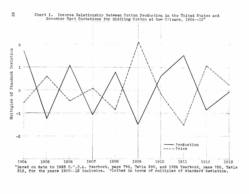
In Chart I on the following page are plotted the data showing the relationship between cotton production and prices. It will be seen that there is a very high degree of -uniformity in movements between the curve representing production of cotton and the curve representing prices. When production rises, prices fall; when production falls, prices rise*Ihis movement of two variables is one type of relationship, known as inverse correlation because of the tendency for production and prices to move in opposite directions. A

Multiples

of Standard

Devi

atio

nOkto Chart I* Inverse Relationship Between Cotton Production in the tfnited States and

November Spot Quotations for Middling Cotton at New Orleans, 1904— 13*

-1

— Production— Price

19081905 1907 19091904 1906 1910 1911 1912 1913*3ased on data in 1923 U.^.P.A. Yearbook, page 796, Table 290, and 1924 Yearbook, page 756, Table 313, for the years 1900— 13 inclusive. Plotted in terms of multiples of standard deviation.

40

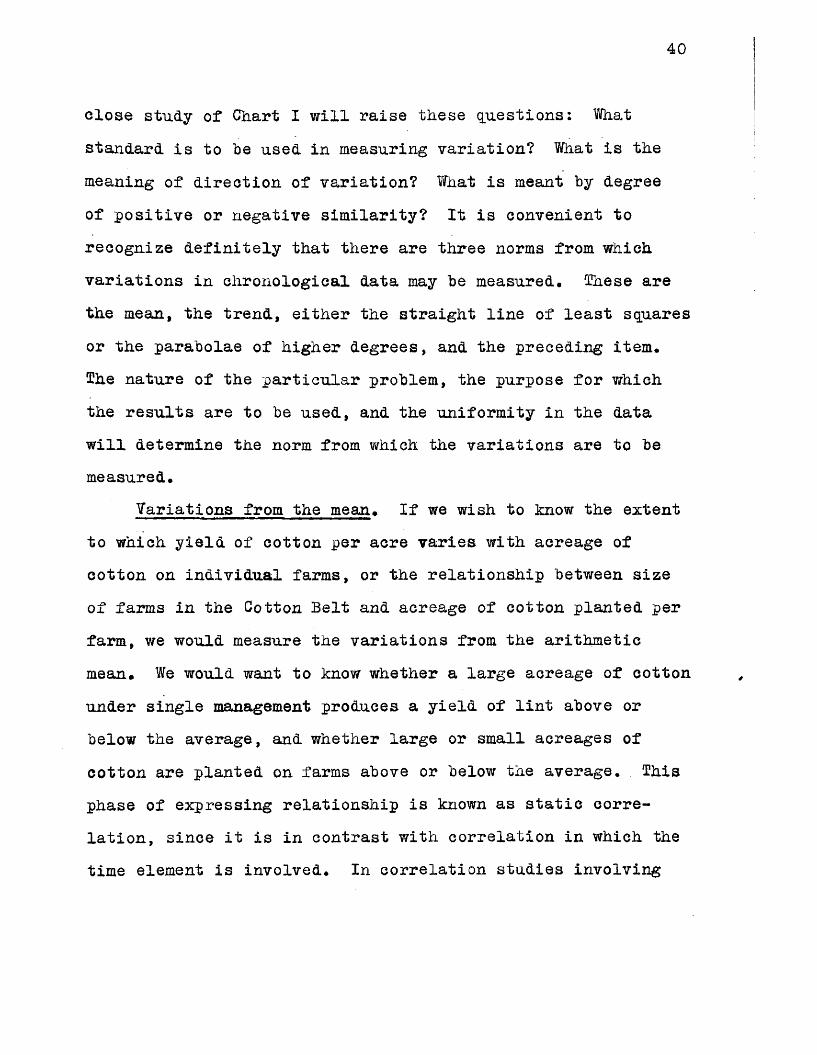
close study of Chart I will raise these questions: Whatstandard is to foe used in measuring variation? What is themeaning of direction of variation? What is meant by degree of positive or negative similarity? It is convenient to recognize definitely that there are three norms from which variations in chronological data may foe measured, These are the mean, the trend, either the straight line of least squares or the parabolae of higher degrees, and the preceding item.The nature of the particular problem, the purpose for which the results are to foe used, and the uniformity in the data will determine the norm from which the variations are to foe measured.

Variations from the mean. If we wish to Know the extent to which yield of cotton per acre varies with acreage of cotton on individual farms, or the relationship between size of farms in the Cotton Belt and acreage of cotton planted perfarm, we would measure the variations from the arithmeticmean. We would want to Know whether a large acreage of cotton under single management produces a yield of lint above or below the average, and whether large or small acreages of cotton are planted on farms above or below the average. This phase of expressing relationship is Known as static corre­lation, since it is in contrast with correlation in which the time element is involved. In correlation studies involving

41

the time element, variations may be measured from the mean of the series if there is no trend, no downward or upward movement, in the data. If there is a trend, then this method of measuring variations often becomes unsatisfactory, inasmuch as the deviations from the means may tend in different degrees to equal zero in the series correlated. 3?his involves the concept that abnormally high or low values may become associated.

Variations from trend, fhe measurement of variations in series from their trends is one of the most important phases of statistical method in economic studies. If it were desired to measure the general character of long-time movement of the original numerical data represented in Chart I, rather than the degree to which prices are influenced by production, a simple method would be to compare the slopes of the secular trends. We would then expect to procure evidence of corre­lation in similar direction, since both production and price show a general tendency to rise. (See Charts II and III).If we are attempting to determine the extent to which series have associated fluctuations, the deviations from the slope of lines of best fit may be used. The comparisons in this case would be with residuals of general movement, which may be represented by either straight lines or lines of higher degree.

42

Deviations from preceding item* There are certain problems in economics in which we are not concerned so ranch with the deviations from the average or trend, but with the deviations from the item immediately preceding. For example, we wish to know if an increase in the price of cotton in December is followed by an increase in cotton planted the next year, or whether an increase in cotton production is followed by an increase or decrease in subsequent monthly prices* In problems of this kind the correlation of first differences is involved, and the actual differences may be correlated, or they may be reduced to percentage changes and multiples of standard deviation. In the latter procedure, the magnitudes would be reduced, and, therefore, the calcu­lations facilitated.

The second problem is that of direction of variation.The relationship between two variables may be direct or inverse. If they tend to fluctuate in the same direction, one increasing when the other increases, and decreasing when the other decreases, we have direct correlation. If one series, however, decreases when the other increases, as in Chart I, we have inverse correlation. We would expect direct correlation between prices of cotton before planting time and acreage of cotton subsequently planted, and inverse corre lation between size of crop and subsequent prices*

43

It is not sufficient to merely state that there is inverse correlation between cotton production and prices.We wish to know whether the relationship is invariable, and whether production and price always vary to the same extent, or if there is a variation in the degree of relative change. The coefficient of correlation may be perfect, high, or low, or there may be no correlation at all. If production and

v*

price, for example, always fluctuate in opposite directions and in constant ratio to each other, there is perfect inverse correlation. If they always move in the same direction, and to the same degree, there is perfect direct correlation. If the fluctuations are such that there is only random associa­tion between them, so that an increase in production is equally likely to be accompanied by either an increase or decrease in price, then there is an absence of correlation.As a faet, many series show some degree of similarity in fluctuations, but very few reach perfection. The problem o'f the statistical analyst is to find some method of measur­ing the extent of similarity. As a measure of this relation­ship the coefficient of correlation has been devised. The computation is such that it reaches plus 1 for perfect direct correlation, minus 1 for perfect inverse correlation, and 0 if there is no relationship. All other expressions range between plus 1 and minus 1.

The Probable Error

In making a statistical analysis of distri­butions which follow the normal law of error it has been found advisable to make use of some measure of dispersion. This is true when we are calculating arithmetic averages as well as when computing correlation coefficients. The measure of dispersion which has been generally employed in such cases is termed the probable error. The name of this measure is derived from the fact that the probability of a given observation vary­ing from the mean of all the observations by an amount greater than the probable error is exactly one-half. It follows that when the observations are arranged in the from of a frequency table in the order of magnitudes an amount equal to the probable error laid off on each side of the arith­metic mean will include one-half of the total number of cases.

This same measure is applied to the coeffi­cients of correlation. If we find that twelve pairs

45

of multiples of standard deviation out of twenty are concurrent, that is, if twelve of the multiples of standard deviation of the Tfyn series are negative, and the corresponding multiples of the nx n series are also negative, and eight divergent, we would presume that the inequality was due entirely, or largely, to chance, but if eighteen pairs were con­current, and only two divergent, the probability of this being due to chance alone would be slight.

Therefore, the probable error of a coefficient of correlation is seen to vary inversely both with the number of pairs of items and with the size of the coefficient. The law of probable error has been calculated by mathematicians and the following formula evolved: P.2. « .6745 (1 - r2). This means that

V~5the coefficient of correlation should always bewritten in the following way: r ■ plus or minus.6745 (1 - r£). When so written, the indications are

7 ~that fifty per cent, of the coefficients similarly calculated will actually lie between r plus or minus .6745 (1 - t Z)

(1)Probable errors of coefficients of correlation calculated from time

series of economic statistical data do not have the usual meaning of probability. Any period selected for the study of historical data is, as a matter of fact, a special period, with definite characteristics distinguishing it from other periods of time. The data, therefore, cannot be considered a random selection, since the individual items in the series are not chosen independently, but rather constitute a succession of items with definite characteristics of conformation.Hence, the probable error of a coefficient of correlation calculated from a time series does not indicate, as might ordinarily be concluded from the theory of probability, that if a coefficient is calculated for any other actual period the chances are equal that it will fall within the range of the coefficient of the first period plus or minus the probable error. The probable error of the coefficient of correlation between time series has no practical significance.

Therefore, the probable errors of the coefficients of correlation in Tables XVIII to Table E, pages 145 to 158, inclusive, and Tables LVI to LIX, pages 224 to 227, inclusive, do not imply the usual meaning of probability, since the data from which they are calculated constitute time series, with their own definite characteristics, and are not random selections.

The fraction *6745 is one-half the distance between quartiles. It is *6745 of the standard deviation. That is to say, the distance from the mean to the qxi&rtile is .6745 of the standard deviation.

47

The Predictive nquation

Coefficients of correlation being calculated, the first step in formulating the predictive equation is to determine the regression coefficient, which is the quantity showing the slope of the line of average relationship between independent and dependent variables. When the relationship is linear the regression equation is a direct derivative of the coefficient of correlation, but when the relationship is non-linear other means are necessarily em­ployed. The regression equation is then developed through specific application of the technic of curve fitting to the original data. In this report the predictive equations are formulated from linear regression relationships.

The coefficient of degression is determined by meansof the following formula: b « r SP.y , in which b - the

SDxregression coefficient, r the coefficient of correlation between the dependent and independent variables, Shy the standard deviation of the dependent variables, and Six the standard deviation of the independent variables. The regression coefficient being determined, the predictive equation may be developed. For this the following formula is used: y = Ay - bhx plus bx, in which the symbolic equivalents

48

are as follows:y = the percentage change in the dependent

variableAy = the arithmetic average of the percentage

changes in the dependent variable b = the coefficient of regression of the dependent

variable on the independent variable x = the percentage change in the independent

variableAx = the arithmetic average of the percentage

changes in the independent variable.Ay - bAx becomes a constant, so that any prediction is the quantity obtained by adding to Ay - bAx the product of the regression coefficient and the percentage change in the in­dependent variable for a particular year.

The concept involved in the formulation of the pre­dictive equation is that for any change in the independent variable there is a corresponding positive or negative change, depending upon the direction of correlation, in the dependent variable.

49

Srror of Estimate

In statistical analysis involving predictions by means of equations formulated from expressions of causal relation­ship , it is always interesting to know the degree of accuracy accompanying the predictions. Ordinarily, the extent to which they can be made varies directly in proportion to the size of the coefficient of correlation, though this is not always the case. If there are abnormally large variables in one series not compensated for in the other, then we may obtain a high expression of relationship which is not a true index of actual cause and effect. This is one of the prob­lems encountered in all methods of correlation, percentage change, sum-product, and others, and equations formulated from the derived regression coefficient in such a case would not be satisfactory in making predictions of any kind.It is only when the coefficient of correlation is an expression of consistent relationship that predictive equations can be evolved from the numerical measure of regression.

By means of the equation y a Ay - Ax plus bx are obtained the normal values of the dependent variable corresponding to the values of each of the given independent variables. The root-mean-square deviations of the actual values from the computed normal values is a measure of dispersion about the

50

line of normal fit, and it is known as the standard error of estimate* In the expression of relationship by the method of determinants the least square residuals of the independent variables are multiplied by their respective weights and summated algebraically to obtain the normal value of the corresponding dependent variable. T h e root- mean-square of actual value deviations from normal values is an expression of reliability of estimate, and it is termed the standard error of estimate. If in a normal curve of estimate a distance equal to the standard error is measured off on each side of the mean the area will include 68 per cent, of the total number of cases, just as in the case of the standard deviation.

51

Shifts and Changes in Cotton Production in the United States,

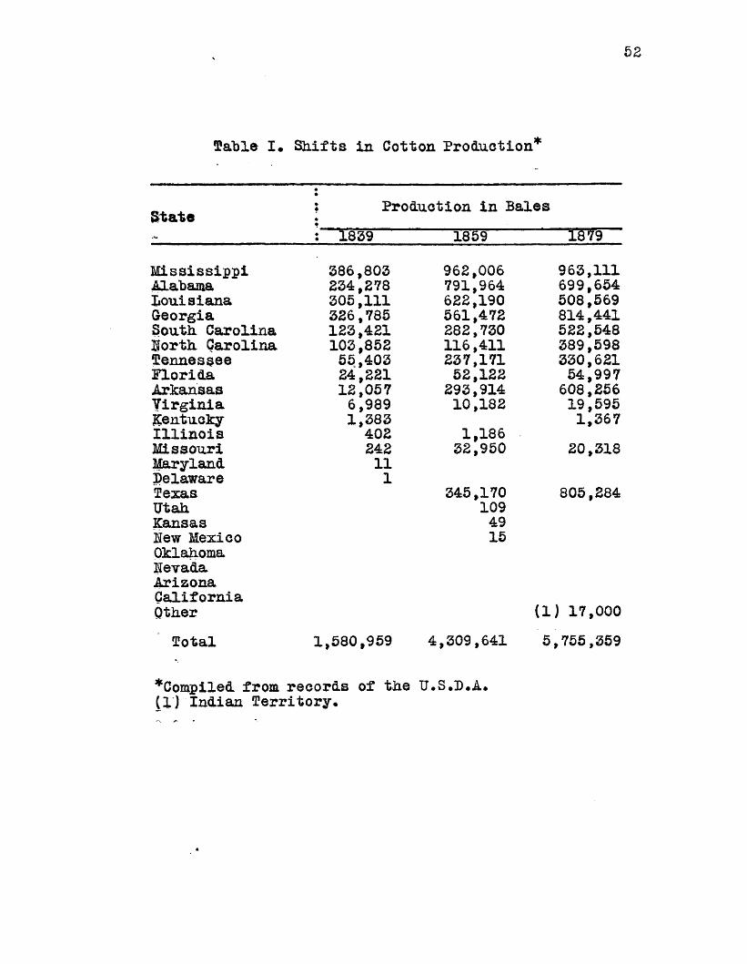
As the cultivable area of the United States has developed and expanded, the production of cotton has moved from the eastern section of the country to the far West. In 1839 cotton was being grown in Maryland and Delaware. Other areas north of those in Which the crop is now grown have been tried out. In fact, prac­tically all available areas for production in the country have been given a trial, in general, climatic factors being considered, the production of cotton increases or decreases with changes in price or pro­fitableness. The shifts and changes in the crop are shown in the accompanying table.

At the time of Whitney1s invention, cotton was being raised in Georgia and South Carolina only Then it spread to North Carolina and Virginia during the early years of the century, and at the outbreak of the second war with England a beginning had been made in Tennessee and louisiana. After the war,

(1) Bogart, Headings in American Economic History.

52

Sable I* Shifts in Cotton Production*

State s Production in Bales: 1839 1859 1879

Mississippi 386,803 962,006 963,111Alabama 234,278 791,964 699,654Louisiana 305,111 622,190 508,569Georgia 326,785 561,472 814,441South Carolina 123,421 282,730 522,548North Carolina 103,852 116,411 389,598Tennessee 55,403 237,171 330,621Florida 24,221 52,122 54,997Arkansas 12,057 293,914 608,256Virginia 6,989 10,182 19,595Kentucky 1,383 1,367Illinois 402 1,186Missouri 242 32,950 20,318Maryland 11Delaware 1Texas 345,170 805,284Utah 109Kansas 49New Mexico 15OklahomaNevadaArizonaCaliforniaQther (1) 17,000Total 1,580,959 4,309,641 5,755,359

*Compiled from records of the U.S.I). A* (1) Indian territory.

53

Table I. (Continued)

State : Production in Bales: 1899 1921 1926

Mississippi 1,286,680 812,867 1,930,000Alabama 1,093,697 579,965 1,490,000Louisiana 699,521 278,805 820,000Georgia 1,232,684 787,052 1,475,000South. Carolina 843,725 754,551 1,030,000Worth Carolina 433,014 776,206 1,250,000Tennessee 235,008 301,949 475,000Florida 53,994 10,905 33,000Arkansas 705,928 796,863 1,620,000Virginia 10,332 16,368 55,000Kentucky 1,371IllinoisMissouri 25,732 69,931 255,000MarylandDelawareTexas 2,584,810 2,197,644 5,900,000Utah 5Kansas 70New Mexico 6 72,000Oklahoma 72,012 481,286 1,950,000Nevada 18Arizona 15 45,323 115,000California 34,109 128,000Other 155,729(1) 8,709 20,000

Total 9,434,345 7,952,539 18,618,000(2)t1) Indian Territory.iSj Revised, figure 17,977,000.

54

Alabama and Mississippi also began to attract attention as cotton-producing areas, and a steady stream of immigrants migrated into those fertile districts•

The United States Department of Agriculture reports that in 1839 the cotton crop occupied only about half the area it now occupies.(This does not refer to acreage} Texas and the Indian Territory west of Arkansas, as is shown, were not producing cotton. East of Texas all of the territory of the Cotton Belt had been opened to occupation by cotton planters, and was being rapidly developed. The addition of large areas of new land that was well suited to the culti­vation of cotton increased production so rapidly in the decade 1839-49 that prices fell to a very low point, notwithstanding this fact, however, production increased 50 per eent. Prices were better during the decade 1849-59, and production continued to increase in all parts of the Cotton Belt, the greatest gains being made in the States of the Southwest. It was

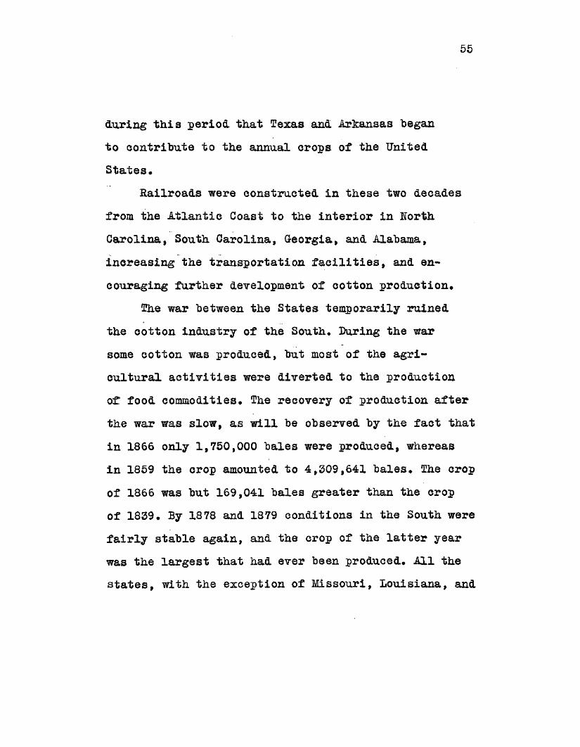
55

during this period that Texas and Arkansas began to contribute to the annual crops or the United States*

Railroads were constructed in these two decades from the Atlantic Coast to the interior in Rorth Carolina, South Carolina, Georgia, and Alabama, increasing the transportation facilities, and en­couraging further development of cotton production*

The war between the States temporarily ruined the cotton industry of the South* During the war some cotton was produced, but most of the agri­cultural activities were diverted to the production of food commodities* The recovery of production after the war was slow, as will be observed by the fact that in 1866 only 1,750,000 bales were produced, whereas in 1859 the crop amounted to 4,309,641 bales* The crop of 1866 was but 169,041 bales greater than the crop of 1839* By 1878 and 1879 conditions in the South were fairly stable again, and the crop of the latter year was the largest that had ever been produced. All the states, with the exception of Missouri, Louisiana, and

56

Alabama produced more cotton that year than in 1859•Between 1879 and 1898 production almost doubled,

increasing from 5,755,359 bales to 11,189,000 bales.In the western states, or rather in the western areas, the increase in production was largely from new lands. The building of railroads in Texas was followed by the development of production in the prairie regions, where grazing and grain farming gave way to cotton. The in­crease in production in the East was largely the result of extensive use of fertilizer on light soils and of improved production methods.

During the decade 1900— 10 Oklahoma and western Texas were more fully developed, adding a large acreage to the cotton producing area, the total acreage in­creasing from 24,933,000 in 1900 to 32,403,000 in 1910. The acreage in 1926 was 47,087,000. From 1914 to 1923 the production of cotton was decreased considerably by the ravages of the boll weevil. The crop in 1915 was 11,192,000 bales, and in 1922 it was 9,755,000, representing an average yearly decline in production of 258,881 bales. The crop of 1921 was only 7,954,000

kales, being the shortest since 1895, when 7,161,000 bales were produced. Since 1922 there has been a general increase in production, The crop of that year was 10,140,000 bales, and in 1926 it reached17,977,000 bales, representing an average yearly increase of 2,791,000 bales.

58

The Cotton Situation in the United. States.Acreage, Production, and Yield per Acre

Prom 1866 to 1926, inclusive, the acreage of cotton har­vested increased more than six times• On an average the yearly increase during the period was 578,000 acres over each preceding year. Following the Civil War there was a rapid economic recovery on the part of the Southern States, and from 1866 to 1890 there was an average increase of 616,000 acres harvested per year.The expansion from 1890 to 1906 was at the rate of 440,000 acres per year, and this was occasioned largely by the westward exten­sion of the cotton-growing areas. From 1906, and until after the World War, the acreage remained fairly constant, and up to 1923 the yearly average increase was only 13,852 acres. In 1923 the acreage harvested increased 4,087,000 over 1922, and from thenuntil 1927 the increase continued gradually, the average for the

000four years, 1923-26, being 3,454, acres per year. This marked upward trend in acreage may be largely attributed to the recovery of prices after 1921 and 1922, which had a tendency to reduce acreages of other crops in the South and to encourage the break­ing up of large ranches in the Southwest*

Production fluctuates with both acreage and yield per acre, and the trend lies between the two. As a rule a large acreage is followed by a large production, though the latter is not always commensurate with the former. In 1914 there were 36,832,000

59

acres of cotton harvested, yielding a total production of16.135.000 hales of lint, the largest crop that had been pro­duced up to that time. Twelve years later, in 1926, 17,977,000 hales, the record crop of the United States, were harvested from47.087.000 acres. It will he observed that the increase in total production did not vary in direct proportion to acreage. The difference was due to yield per acre, which was 209.2 pounds in 1914, and 182*5 pounds in 1926.

From 1866 to 1890 production increased at the yearly average rate of 238,000 hales. After 1890, and up to 1906, there was a slight tendency toward decrease in production, the yearly average rate of increase heing only 234,000 hales. Following 1905, and continuing until 1921, there was a marked decrease in total pro­duction, the yearly average decline heing at the rate of 17,000 hales. The seasons of 1921 and 1922 were the poorest4that had been experienced for many years, the crop of 1921 heing the shortest since 1895. Uuring the four years following 1922 the production increased at the rate of 2,600,000 hales per year.This was due to both the extensive increase in acreage and to the very marked increase in yield per acre.

From year to year the yields per acre fluctuate greatly,, due mainly to boll-weevil infestation and to adverse weather conditions, which, incidentally, may be favorable to boll-weevil activity. The trend from 1866 to 1890 was downward at the rate

60

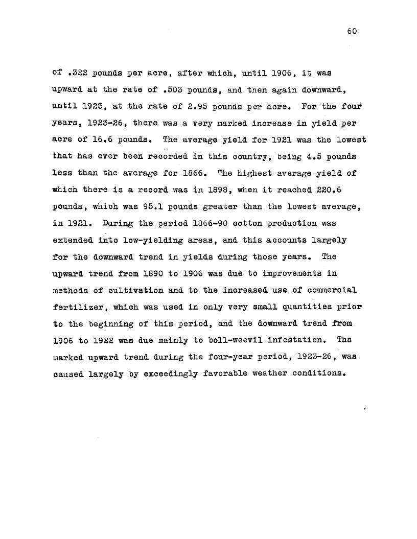
of .322 potm&s per acre, after which., until 1906, it was upward at the rate of *503 pounds, and then again downward, until 1923, at the rate of 2.95 pounds per aore. For the four years, 1923-26, there was a very marked increase in yield per acre of 16.6 pounds. The average yield for 1921 was the lowest that has ever heen recorded in this country, heing 4.5 pounds less than the average for 1866. The highest average yield of which there is a record was in 1898, when it reached 220.6 pounds, which was 95.1 pounds greater than the lowest average, in 1921. During the period 1866-90 cotton production was extended into low-yielding areas, and this accounts largely for the downward trend in yields during those years. The upward trend from 1890 to 1906 was due to improvements in methods of cultivation and to the increased use of commercial fertilizer, which was used in only very small quantities prior to the beginning of this period, and the downward trend from 1906 to 1922 was due mainly to boll-weevil infestation. Ths marked upward trend during the four-year period, 1923-26, was caused largely by exceedingly favorable weather conditions.

61

Table II* Acreage, Production, and Yield per Acre of Cotton in the United States, 1866---1926*

Year Acres Production Yield per Acre(1,000) (1,000 bales) (lbs)

1866 7,599 1,750 129*01867 7,828 2,340 189*81868 6,799 2,380 192.21869 7,743 3,012 196.91870 8,885 3,800 198.91871 7,558 2,553 148.21872 8,483 3,920 188.71873 9,510 3,683 179.71874 11,764 3,941 147.51875 11,934 5,123 190.61876 11,677 4,438 167.81877 12,133 4,370 163.81878 12,344 5,244 191.21879 14,480 5,755 181.01880 15,951 6,343 184.5^Yearbook of the U.S.D.A., 1919, page 590, Table 125and 1926, page 962, Table 235*

Year

18811883188318841885188618871888188918901891189318931894189518961897

63

Table II • (Continued.)

Acres Production Yield per Acre(1,000) (1,000 bales) (lbs)

16,711 5,456 149*816,377 6,957 185.716,778 5,701 164.817,440 5,683 153.818,301 6,575 164.418,455 6,447 169.518,641 7,030 183.719,059 6,941 180.430,175 7,473 159.719,513 8,674 187.019,059 9,618 179.415,911 6,664 309.319,535 7,493 149.933,688 9,476 195.330,185 7,161 155.633,373 8,533 184.934,330 10,898 183.7

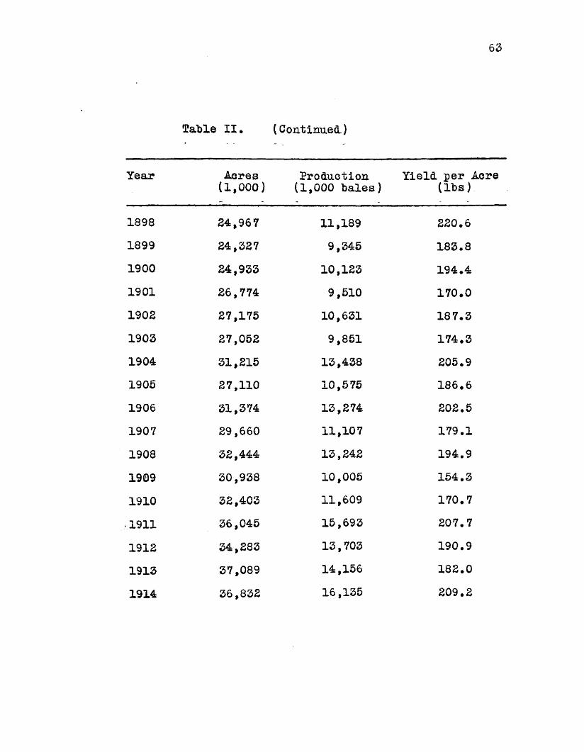
63

3?able IX • (Continued)

Year Acres Production Yield per Acre(1,000) (1,000 bales) (lbs)

1898 24,967 11,189 220.61899 24,327 9,345 183.81900 24,933 10,123 194.41901 26,774 9,510 170.01902 27,175 10,631 187.31903 27,052 9,851 174.31904 31,215 13,438 205.91905 27,110 10,575 186.61906 31,374 13,274 202.5190? 29,660 11,107 179.11908 32,444 13,242 194.91909 30,938 10,005 154.31910 32,403 11,609 170.71911 36,045 15,693 207.71912 34,283 13,703 190.91913 37,089 14,156 182.01914 36,832 16,135 209.2

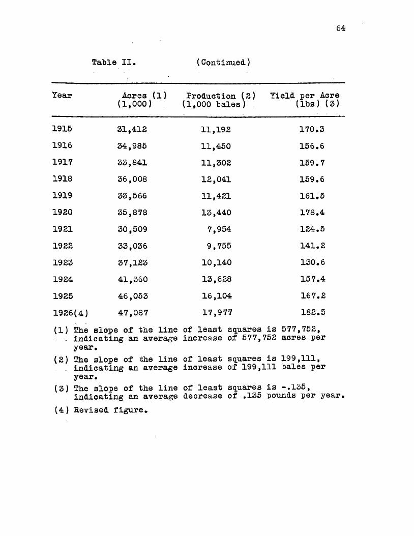
64

Table II* (Continued)

Year Acres (1) (1,000)

Production (2) (1,000 bales)

Yield per Acre (lbs) (3)

1915 31,412 11,192 170.31916 34,985 11,450 156.61917 33,841 11,302 159.71918 36,008 12,041 159.61919 33,566 11,421 161.51920 35,878 13,440 178.41921 30,509 7,954 124.51922 33,036 9,755 141.21923 37,123 10,140 130.61924 41,360 13,628 157.41925 46,053 16,104 167.21926(4) 47,087 17,977 182.5(1) The slope of the line

- indicating an averageof least squares increase of 577,

is752

577,752, acres per

year(2) The slope of the line - . indicating an average

of least squares increase of 199,:

is111

199,111, bales per

year► ̂

(3) The slope of the line indicating an average

of least squares decrease of *135

is -*135, pounds per year.

(4) Revised figure.

65

Comparison of Cotton Production in the United States and Other Leading Countries#

2?he United States is the most important cotton** producing country in the world, the average production "being more than half the total world product# The other leading countries in the order of their importance are India, China, Egypt, and Brazil#

India is characterized "by erude methods of pro­duction and lack of sufficient rainfall in the cotton regions, so that the average yield per acre is less than half that of the United States. Por the period 1900— £6 inclusive the average yield per acre in India was 79#6 pounds, while for the same period the average yield in the United States was 173.8 pounds# The sta­tistics for China present so many apparent inaccuracies that a comparison of the yields with those of the United States is being purposely omitted# Egypt, the fourth largest producer, maintained an average of384.4 pounds per acre for the period 1900-87, inclusive, as compared with an average of 167.1 pounds for the United States, while Brazil, the fifth country in

66

importance, produced an average yield of £07.6 pounds per acre during the period 1911— 26, inclusive, and the average production per acre in the United States for the same period was 168.4 pounds.

Ihe total production of cotton in India for the years 1900-26,inclusive, was 29.3 per cent, as great as the production in the United States. Egypt, during the period 1900-27,inclusive, produced 10.7 per cent, as much cotton as the United States, while Brazil, during the period 1911-26,inclusive, reported a pro­duction 3.6 per cent, as great as that of the United States for the same years*

As will be observed in the accompanying tables, the yield per acre in India is extremely low, while that of Egypt is high as compared with the yield in the United States. For the period 1900-26 inclusive , the yield per acre in India was 45.7 per cent, as great as the yield in the United States, while in Egypt for the period 1900-27, inclusive,it was 130 per cent, greater, and in Brazil during the period 1911-26#inclusive »the yield per acre was 23.3 per cent, greater than the yield in the United States.

67

Table III* Comparison of Cotton Acreage Harvested in the Unite! States,

India, and Egypt, 1900-27*

Year : Thousands of Acres: United States India Egypt

1900 24,933 14,231 1 2771901 26,774 14,506 1 2981902 27,175 16,581 1 3241903 27,052 18,205 1 3841904 31,215 19,918 1 4921905 27,110 21,072 1 6271906 31,374 22,484 1 5631907 29,660 21,630 1 6641908 32,444 19,999 1 7021909 30,938 21,005 1 6581910 32,403 23,040 1 7051911 36,045 21,415 1 7671912 34,283 22,028 1 7871913 37,089 25,027 1 7881914 36,832 24,595 1 8221915 31,412 17,773 .1 2311916 34,985 21,771 1 7191917 33,841 25,337 1 7411918 36,008 21,037 1 3661919 33,566 23,383 1 6341920 35,878 21,339 1 8971921 30,509 18,451 1 3391922 33,036 21,804 1 8691923 37,123 23,631 1 7801924 41,360 26,801 1 8561925 46,053 28,491 1 9981926 47,087 24,976 1 8541927 40,168 1 574^Compiled from records of the U*S.D.A*Slope of line of least squares:

United States 526,454India 297,123Egypt 22,797

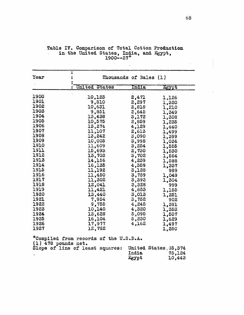
68

Table IV* Comparison of Total Cotton Production in.the.United. States, India, and Egypt,

1900— 27*

Year : Thousands of Bales (1): Ohited States India ferpt

1900 10,123 2,471 1,1261901 9,510 2,297 1,3201902 10,631 2,818 1,2101903 9,851 2,645 1,3491904 13,438 3,172 1,3081905 10,575 2,859 1,2351906 13,274 4,129 1,4401907 11,107 2,613 1,4991908 13,242 3,090 1,3991909 10,005 3,998 1,0361910 11,609 3,254 1,5551911 15,693 2,730 1,5301912 13,703 3,702 1,5541913 14,156 4,239 1,5881914 16,135 4,359 1,3371915 11,192 3,128 9891916 11,450 3,759 1,0491917 11,302 3,393 1,3041918 12,041 3,328 9991919 11,421 4,853 1,1551920 13,440 3,013 1,2511921 7,954 3,752 9021922 9,755 4,245 1,3911923 10,140 4,320 1,3531924 13,628 5,095 1,5071925 16,104 5,230 1,6291926 17,977 4,162 1,4971927 12,782 1,250Compiled, from records of tde U.S.P.A.(1) 478 pounds net.Slope of line of least squares: United States 3 5 ,374

India 75,124Sgypt 10,443

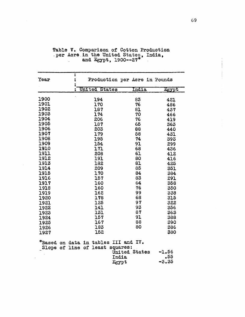
69

fable V. Comparison of Cotton Production .per Acre in the United. States, India,

and Egypt, 1900— 27*

Year+••♦*

Production per Acre in Pounds: United. States India Egypt

1900 194 83 4211901 170 76 4861902 187 81 4371903 174 70 4661904 206 76 4191905 187 65 3631906 203 88 4401907 179 58 4311908 195 74 3931909 154 91 2991910 171 68 4361911 208 61 4121912 191 80 4161913 182 81 4251914 209 85 3511915 170 84 3841916 157 83 2911917 160 64 3581918 160 76 3501919 162 99 3381920 178 68 3151921 125 97 3221922 141 93 3561923 131 87 3631924 157 91 3881926 167 88 3901926 183 80 3861927 152 380*Based on data in tables III and IT*Slope of line of least squares ••

United States -1.56India .55Egypt -3.35

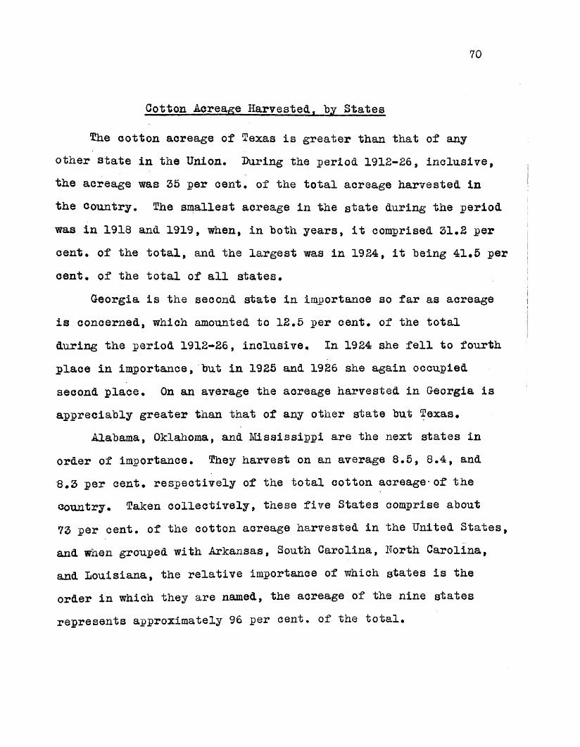
70

Cotton Acreage Harvested., by States

The cotton acreage of Texas is greater than that of any other state in the Union* Ihxring the period 1912-26, inclusive, the acreage was 35 per cent* of the total acreage harvested in the country. The smallest acreage in the state during the period was in 1918 and 1919, when, in both years, it comprised 31.2 per cent* of the total, and the largest was in 1924, it being 41.5 per cent, of the total of all states.

Georgia is the second state in importance so far as acreage is concerned, which amounted to 12.5 per cent, of the total during the period 1912-26, inclusive. In 1924 she fell to fourth place in importance, but in 1925 and 1926 she again occupied second place* On an average the acreage harvested in Georgia is appreciably greater than that of any other state but Texas.

Alabama, Oklahoma, and Mississippi are the next states in order of importance. They harvest on an average 8.5, 8.4, and 8.3 per cent, respectively of the total cotton acreage-of the country. Taken collectively, these five States comprise about 73 per cent, of the cotton acreage harvested in the United States, and when grouped with Arkansas, South Carolina, North Carolina, and Louisiana, the relative importance of which states is the order in which they are named, the acreage of the nine states represents approximately 96 per cent, of the total.

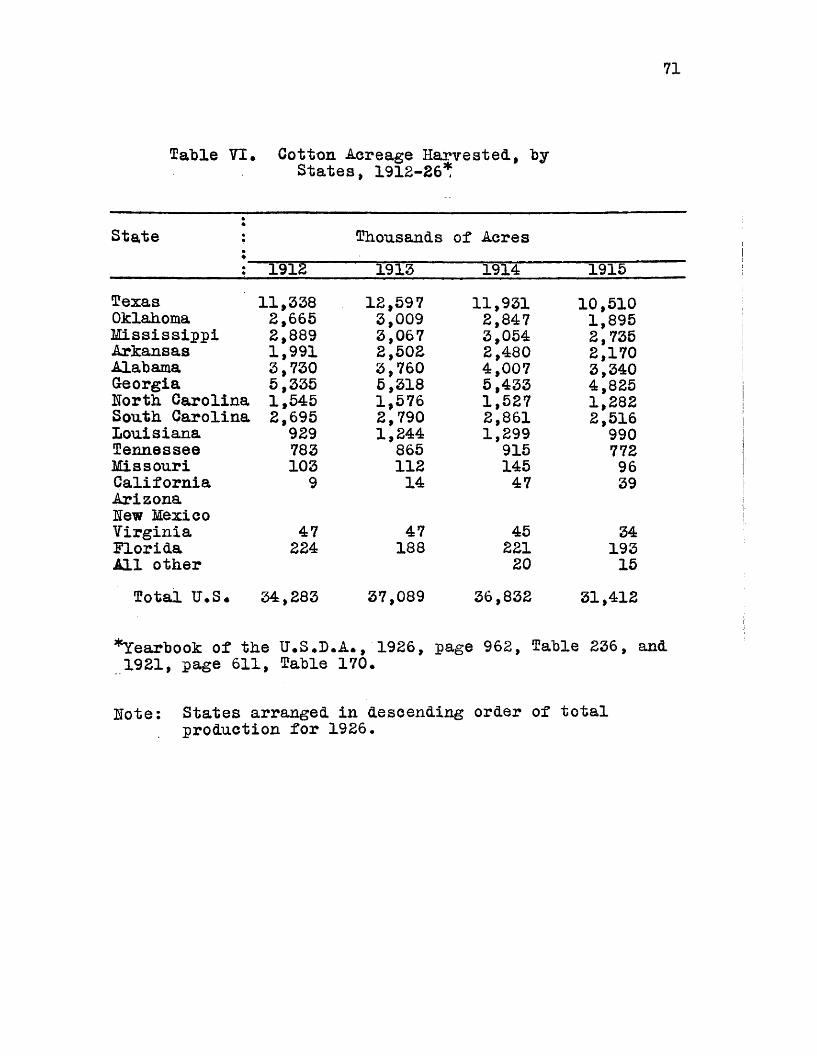
71

Table VI. Cotton Acreage Harvested., by States, 1912-26*

State : Thousands of Acres•* 1912 1913 1914 1915

Texas 11,338 12,597 11,931 10,510Oklahoma 2,665 3,009 2,847 1,895Mississippi 2,889 3,067 3,054 2,735Arkansas 1,991 2,502 2,480 2,170Alabama 3,730 3,760 4,007 3,340Georgia 5,335 5,318 5,433 4,825Uorth Carolina 1,545 1,576 1,527 1,282South Carolina 2,695 2,790 2,861 2,516Louisiana 929 1,244 1,299 990Tennessee 783 865 915 772Missouri 103 112 145 96California 9 14 47 39ArizonaHew MexicoVirginia 47 47 45 34Florida 224 188 221 193All other 20 15

Total IT*S. 34,283 37,089 36,832 31,412

*Yearbook of the U*S*I)*A*, 1926, page 962, Table 236, and 1921, page 611, Table 170*

Hote: States arranged in descending order of totalproduction for 1926.

72

Table VI• (Continue!)

State : Thousands of Acres~___________________ 1916 1917 1918 1919 '

11,233 10,476TexasOklahomaMississippiArkansasAlabamaGeorgiaitorth CarolinaSouth CarolinaLouisianaTennesseeMissouriCaliforniaArizonaHew MexicoVirginiaFloridaAll other

Total U.S*

11,400 11,0922,562 2,7833,110 2,7882,600 2,7403,225 1,9775,277 5,1961,451 1,5152,780 2,8371,250 1,454

887 882133 15352 136

4142 50191 18325 15

34,985 33,841

2,998 2,4243,138 2,8482,991 2,7252,570 2,7915,341 5,2201,600 1,4903,001 2,8351,683 1,527902 758148 12585 8595 10744 42167 10312 10

36,008 33,566

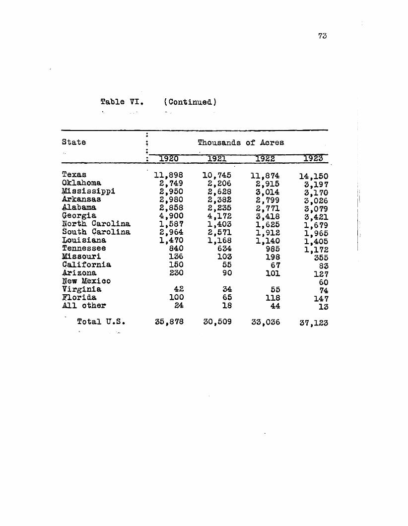
73

Table VI* (Continued)

State Thousands of Acres: 19&0 1921 1922 1923“

Texas 11,898 10,745 11,874 14,150Oklahoma 2,749 2,206 2,915 3,197Mississippi 2,950 2,628 3,014 3,170Arkansas 2,980 2,382 2,799 3,026Alabama 2,858 2,235 2,771 3,079Oeorgia 4,900 4,172 3,418 3,421Uorth Carolina 1,587 1,403 1,625 1,679South Carolina 2,964 2,571 1,912 1,965Louisiana 1,470 1,168 1,140 1,405Tennessee 840 634 985 1,172Missouri 136 103 198 355California 150 55 67 83Arizona 230 90 101 127lew Mexico 60Virginia 42 34 55 74Florida 100 65 118 147All other 24 18 44 13Total U.S. 35,878 30,509 33,036 37,123

74

fable VI# (Continued)

State : Thousands of Acres1924 1925 1926

Texas 17,175 17,608 18,363Oklahoma 3,861 5,214 4,912Mississippi 2,981 3,466 3,768Arkansas 3,094 3,738 3,782Alabama 3,055 3,504 3,713Georgia 3,046 3,589 4,029Horth Carolina 2,005 2,017 2,023South Carolina 2,404 2., 654 2,732Louisiana 1,616 1,874 1,960Tennessee 996 1,173 1,178Missouri 493 520 488California 130 169 160Arizona 180 162 167Hew Mexico 101 107 120Virginia 102 100 101Florida 80 101 109All other 41 57 48Total U*S« 41,360 46,053 47,653;(1)

(l)The revised figure for 1926 is 47,087

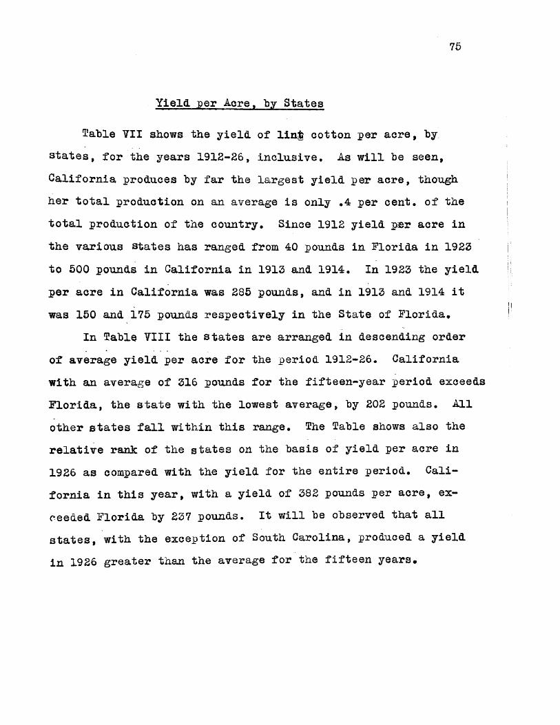
75

Yield, per Acre, by States

Table VII shows the yield, of lint cotton per acre, by. states, for the years 1912-26, inclusive. As will be seen, California produces by far the largest yield per acre, though her total production on an average is only .4 per cent, of the total production of the country. Since 1912 yield per acre in the various states has ranged from 40 pounds in Florida in 1923 to 500 pounds in California in 1913 and 1914. In 1923 the yield per acre in California was 285 pounds, and in 1913 and 1914 it was 150 and 175 pounds respectively in the State of Florida.

In Table VIII the states are arranged in descending order of average yield per acre for the period 1912-26. California with an average of 316 pounds for the fifteen-year period exceeds Florida, the state with the lowest average, by 202 pounds. All other states fall within this range. The Table shows also the relative rank of the states on the basis of yield per acre in 1926 as compared with the yield for the entire period. Cali­fornia in this year, with a yield of 382 pounds per acre, ex­ceeded Florida by 237 pounds. It will be observed that all states, with the exception of South Carolina, produced a yield in 1926 greater than the average for the fifteen years.

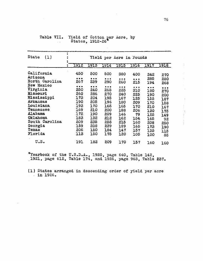
76

Table 711. Yield of States,

Cotton per 1912-26

Acre, by

State (1) Yield per Acre in Founds1912 1913 1914 1915 1916 1917 1918

California 450 500 500 380 400 242 270Arizona ... ... ... ... ... 285 280Horth Carolina 267 239 290 260 215 194 268Hew Mexico ... ... ... * • •Virginia 250 240 265 225 310 • • •180 • • •

270Missouri 260 286 270 240 225 190 200Mississippi 173 204 195 167 125 155 187Arkansas 190 205 196 180 209 170 158Louisiana 193 170 165 165 170 210 167Tennessee 169 210 200 188 206 130 175Alabama 172 190 209 146 79 125 149Oklahoma 183 132 212 162 154 165 92South Carolina 209 235 255 215 160 208 250Georgia 159 208 239 189 165 173 190Texas 206 150 184 147 157 135 115Florida 113 150 175 120 105 100 85U.S. 191 182 209 170 157 160 160

^Yearbook of the U.S.L.A. , 1920 , page 640, Table 142,1921, page 612, Table 174, and 1926 > page 963, Table 237.

(1) States arranged in descending order of yield per acre - in 1926.

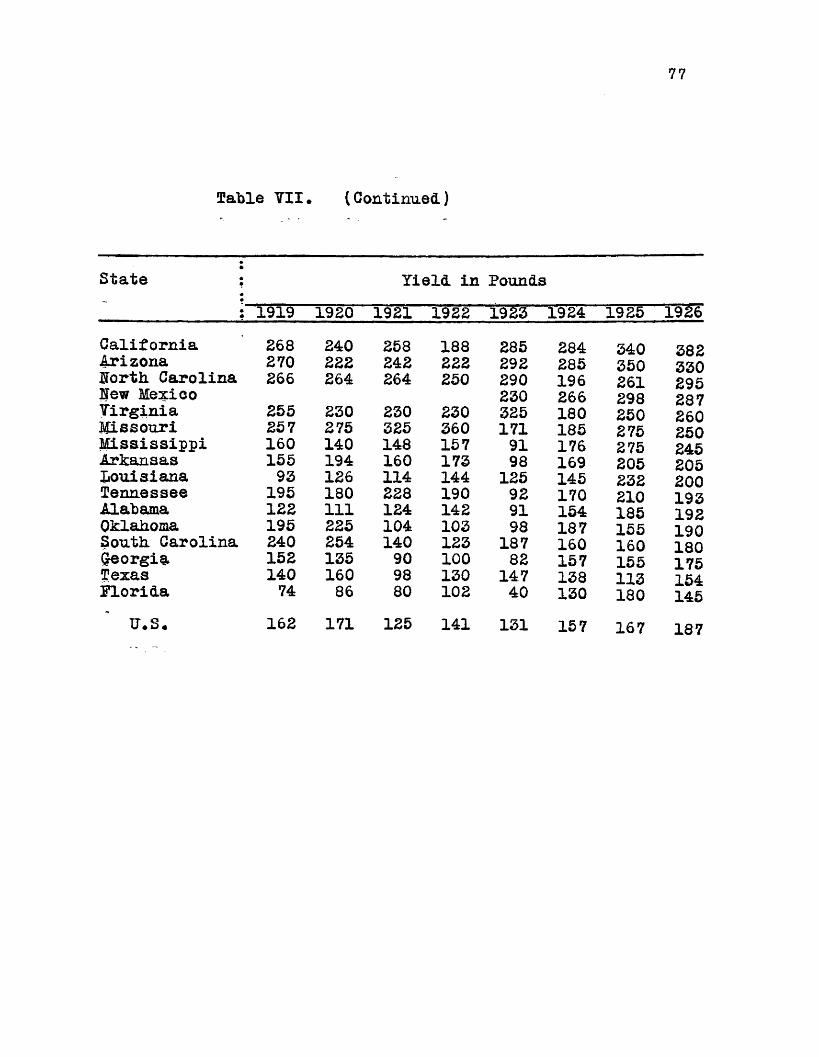
77

Table VII. (Continued)

State : Yield in Pounds' 1 1919 1920 X92l 1522 1523 1521 1925 1926California 268 240 258 188 285 284 340 382Arizona 270 222 242 222 292 285 350 330Uorth Carolina 266 264 264 250 290 196 261 295Hew Mexico 230 266 298 287Virginia 255 230 230 230 325 180 250 260Missouri 257 275 325 360 171 185 275 250Mississippi 160 140 148 157 91 176 275 245Arkansas 155 194 160 173 98 169 205 205Louisiana 93 126 114 144 125 145 23 2 200Tennessee 195 180 228 190 92 170 210 193Alabama 122 111 124 142 91 154 185 192Oklahoma 195 225 104 103 98 187 155 190South Carolina 240 254 140 123 187 160 160 180Qeorgia 152 135 90 100 82 157 155 175Texas 140 160 98 130 147 138 113 154Florida 74 86 80 102 40 130 180 145

U.S. 162 171 125 141 131 157 167 187

78

Table 71II# Average Yield of Cotton per Acre, by States, for the Period 1912— 26 and

for the Year 1926*

State Average 1912-26 Year 1926

Yield in lbs. Rank Yield in lbs. Rank

Calif. 316 1 382 1Ariz. 277 2 330 2N. C. 256 3 295 3N. M. 182 7 287 47a. 247 4 260 5Mo. 242 5 250 6Miss. 176 9 245 7Ark. 162 12 205 8la. 164 10 200 9Tenn. 181 8 193 10Ala. 150 14 192 11Okla. 159 13 190 12S. C. 203 6 180 13Ga. 163 11 175 14Tex. 145 15 154 15Fla. 114 16 145 16Average for the period 1912-26 computed from data in 1926 U.S.D.A. Yearbook, page 963, table 238, and page 962, table 236; 1921 Yearbook, page 611, table 171, and page 611, table 170.Note: For New Mexico the average yield per acre for the

period 1912-26 is based on four years only, 1923-to 1926^ inclusive.,For Arizona the average yield per acre for the period 1912-26 is based on ten years, 1917 to 1926 inclusive.

79

Total Production. by States

Production of lint cotton in the United States during the fifteen-year period, 1912-26, has ranged from 7,954,000 bales in 1921 to 17,977,000 bales in 1926. Table IX shows the pro­duction by states and for the country as a whole, Texas ranks first in importance, the total production for the period being 30,6 per cent, of the total of all states, Georgia, with 12,2 per cent, of the total production, is the second in order, and Mississippi and South Carolina, eaeh with 8.8 per cent., rank third. These four states during the period 1912-26 produced 60 per cent, of the total crop of the country. Arkansas, Oklahoma, Alabama, and Horth Carolina are next in importance in the order named. Their combined production represents approximately 31 per cent, of the total of all states, which when added to the production of Texas, Georgia, Mississippi, and South Carolina comprises 91 per cent, of all the cotton produced in the United States. It will be seen, therefore, that cotton production in this country, so far as final ginnings are concerned, is confined almost exclusively to eight states.

80

Table IX. Production of Lint Cotton in 500 Pound Gross Weight Bales, by

States, Year Beginning with August, 1912-26*

State 2 Production in Thousands of Bales (l)i

: 1912 1913 1914 1915 1916Texas 4,880 3,945 4,592 3,227 3,726Oklahoma 1,021 840 1,262 640 824Mississippi 1,046 1,311 1,246 954 812Arkansas 792 1,073 1,016 816 1,134Alabama 1,342 1,495 1,751 1,021 533Georgia 1,777 2,317 2,718 1,909 1,821Uorth Carolina 866 792 931 699 655South Carolina 1,182 1,378 1,534 1,134 932Louisiana 376 444 449 341 443Tennessee 277 379 384 303 382Missouri 56 67 82 48 63California Arizona new Mexico

8 23 50 29 4:4

Yirginia 24 23 25 16 27Florida 53 59 81 48 41All other 3 10 14 7 14Total U.S* 13,703 14,156 16,135 11,192 11,450

*Yearbook of the U.S.L^A*, 1921, page 611, Table 171, and 1926, page 963, Table 238.(1) Excluding linters*(2) Production of individual States totals 11,451.Hote: States arranged in descending order of production

for 1926.

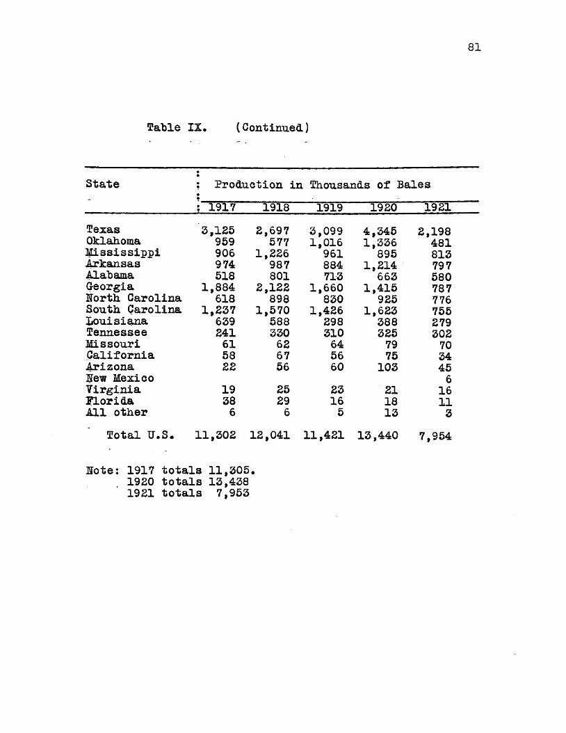
81

Table IX* (Continued)

State Production in Thousands of Bales: 1917 1918 1919 1920 1921

Texas 3,125 2,697 3,099 4,345 2,198Oklahoma 959 577 1,016 1,336 481Mississippi 906 1,226 961 895 813Arkansas 974 987 884 1,214 797Alabama 518 801 713 663 580Georgia 1,884 2,122 1,660 1,415 787Horth Carolina 618 898 830 925 776South Carolina 1,237 1,570 1,426 1,623 755Louisiana 639 588 298 388 279Tennessee 241 330 310 325 302Missouri 61 62 64 79 70California 58 67 56 75 34Arizona 22 56 60 103 45Hew Mexico 6Virginia 19 25 23 21 16Florida 38 29 16 18 11All other 6 6 5 13 3Total U.S. 11,302 12,041 11,421 13,440 7,954

Uote: 1917 totals 11,305.1920 totals 13,4381921 totals 7,953

Table IX. (Continued)

State : Production in Thousands of Balesr

1 9 2 2 1 9 2 3 1924 1 9 2 5 1 9 2 6Texas 3,222 4,340 4,949 4,163 5,900Oklahoma 627 656 1,511 1,691 1,950Mississippi 989 604 1,099 1,991 1,930Arkansas 1,012 622 1,094 1,600 1,620Alabama 823 587 985 1,357 1,490Georgia 715 588 1,002 1,164 1,475Horth Carolina 852 1,020 825 1,102 1,250South Carolina 492 770 807 889 1,030Louisiana 343 368 493 910 820Tennessee 391 226 354 515 475Missouri 149 127 193 299 255California 21 54 77 122 128Arizona 47 78 108 119 115Hew Mexico 12 30 57 66 72Virginia 27 51 39 53 55Florida 25 12 22 38 33All other 7 8 14 26 20

Total U.S. 9,755 10,14 0 13,628 16,104 18,618(1) Revised, figure 17,977.Rote: 1922 totals 9,744.

1923 totals 10,141.1924 totals 13,629.1925 totals 16,105.

83

Cotton ffxports

Since 1866, when we exported 75.6 per cent, of our domestic production, foreign consumption of American cotton has "been in­creasing, Over the entire sixty-year period, 1866-1925, this increase has been at the rate of 96,000 bales per year. The increase was fairly constant until 1915, when exports declined rather sharply, and continued to decline until the season of 1919. During the World War, 1914-18, our domestic consumption increased at an average rate of approximately 50,000 bales per year, and exports decreased during the same period at an average rate of 775,000 bales per year. The decrease in exports may be attributed to the disturbance of trade conditions abroad and to the increased exportation from the United States of manufactured fabrics. Table X shows the trend of exports from 1866 to 1926. On an average we export 60 per cent, of the total cotton pro­duction, which ranks first in value among all of our exported commodities. From 1900 to 1919 we exported 66 per cent, of the crop, and since 1919, including the year 1926, our exports amounted to 55 per cent, of the total production. A comparison of Tables II and X will show that the years of large crops have been associated with large exports from the United States, with the exception of 1914, the first year of the World War. This tendency for record crops to be followed by correspondingly

84

large exports may "be explained by the fact that domesticconsumption cannot be increased in the same ratio as the crop

isincreases. This/shown by the fact that for the years 1921-25, inclusive, our domestic production increased at the yearly rate of 2,017,000 bales, while domestic consumption during the same period increased at the rate of only 61,000 bales per year. Associated with the increase in production was a yearly average increase in exports of 690,000 bales. The difference between production and consumption and exports constituted the annual carry-over. This, together with the fact that years of short crops are ordinarily associated with a decrease in exports, indicates that changes in crops are reflected more in volume of exports than in domestic consumption.

Europe is the greatest buyer of American cotton exports.In 1926*81.7 per cent, of the domestic production passing into the world’s channels of trade as lint cotton entered the European markets. The United Kingdom, the greatest individual buyer, took 28.1 per cent, of our exports in 1926, Germany,20.4 per cent., Japan, 13.8 per cent., France, 11.4 per cent., and Italy, 9.2 per cent.

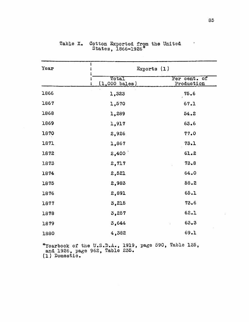
85

Table Z. Cotton Exported from the United States, 1866-1926*

Year Exports (1)Total Per cent* of

(1,000 bales)_____________Production1866 1,323 75.6i1867 1,570 67.11868 1,289 54.21869 1,917 63.61870 2,926 77.01871 1,867 73.11872 2,400 ' 61.21873 2,717 73.81874 2,521 64.01875 2,983 58.21876 2,891 65.11877 3,215 73.61878 3,257 62.11879 3,644 63.31880 4,382 69.1

^Yearbook of tiie U.S and 1926, page 962, (1) Domestic.

.D.A., 1919, page 590, Table 235.

Table 125

86

Ta"ble X, (Continued)

Year••: Exports♦ft: 3?otal : (1,000 "bales)

Per cent, of Production

1881 3,481 63.81882 4,576 65.81883 3,725 65.31884 3,783 66.61885 4,116 62.61886 4,339 67.31887 4,529 64.51888 4,770 c-.00<£>

1889 4,944 66.21890 5,815 67.01891 5,870 61.01892 4,424 66.41893 5,367 71.61894 7,035 74.21895 4,670 65.21896 6,208 72.8189 7 7,726 70.9

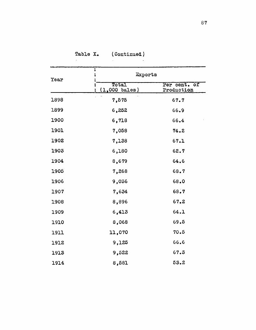
Year

18981899190019011902190319041905190619071908190919101911191219131914

87

Sable X. (Continue!)

Exportsfotal

(1,000 bales)Per cent* of Production

7,5756,2526,7187,0587,1386,1808,6797,2689,0367,6348,8966,4138,068

11,0709,1259,5228,581

67*766*966.4 74.267.1 62.764.668.7 68.068.767.264.169.570.566.667.353.2

88

Table X. (Continued)

Year : Exports: Total : (1,000 bales)

Per cent, of Production

1915 5,917 52.91916 5,702 49.81917 4,455 39.41918 5,442 45.21919 7,036 61.61920 5,570 41.41921 6,592 82.91922 5,206 53,41923 5,784 57.01924 8,239 60.51925 8,110 50.41926 (1) 8,292 44 . 6(l) Estimated.

The slope of the line of least squares for the period 1866 to 1925, inclusive, is 96,053, meaning that on an average the exports have increased 96,053 bales a year. In computing the line of least squares the figure for 1926 has been omitted. Since the War, up to and including the year 1926, we have exported 55 per cent, of our total pro­duction. Up to the end of the War, that is, from 1900 to 1918, inclusive, we had exported on an average 66 per cent, of the total production, and from 1900 to the present time our exports have amounted to 60 oer cent, of the production.

89

Table XI* Destination of Domestic Cotton Exports, 1924-26*

Country to which exported j Exports in 500 pound bales (1)

: 1924 1925 1926United Kingdom 1,685,377 2,605,456 2,278,372Germany 1,271,738 1,765,673 1,657,070France 738,841 932,866 927,184Italy 559,833 747,594 742,677Other Europe 764,695 1,089,700 1,019,018Japan 583,957 849,584 1,118,246Other Countries 179,258 247,944 366,977

Total 5,783,699 8,238,817 8,109,544Total Europe 5,020,484 7,141,289 6,624,321

^Yearbook of the U*S.D*A*, 1926, page 1185, Table 498

(1) Excluding linters, for year ending June 30th*

90

Cotton Imports

Hie net imports of ootton into the United States during the five-year period, 1921-25, were equivalent to 5.5 per cent, of the total quantity of cotton consumed in the country, ex­clusive of linters. Ihe largest annual ratio during this periodwas 6.0 per cent., in 1921, and the smallest was 4.8 per cent.,. 11 )m 1925 • Ihese small amounts are "brought in for special purposes. Most of the imported cotton is long-staple Egyptian, which is used largely in the manufacture of knit goods, lace, automobile tires, and thread.

lable XIII shows the principal countries from which the United States imports. As will be seen, Mexico ranks next to Egypt in importance as a source of supply, with China third, and Peru fourth. Over the entire period, 1867-1925, our imports have increased at the yearly average rate of 7,342 bales, fhere is no causal relationship between the size of the domestic crop in this country and the volume of imports. Most of the lint cotton bought by American manufacturers from foreign countries is used for purposes in which the American short—staple grades cannot be substituted, and, therefore, a short crop in the United States is equally likely to be followed by either an increase or decrease in imports.

(l)JToreign Crops and Markets, Volume 13, lumber 19, Nov. 8, 1926, page 624.

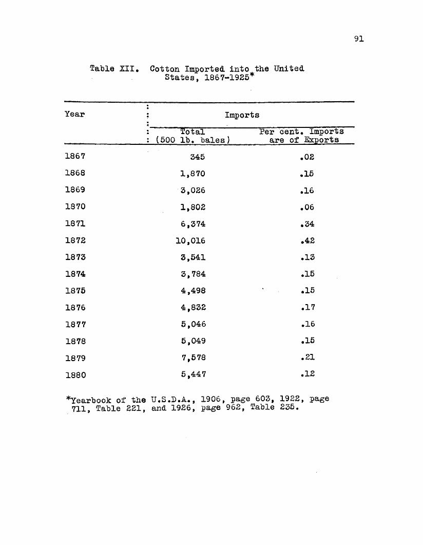
91

Table XII* Cotton Imported into the UnitedStates, 1867-1925*

Year ; Imports: Total Per cent* Imports : (500 lb. bales) are of Exports

1867 345 .021868 1,870 *151869 3,026 .161870 1,802 .061871 6,374 .341872 10,016 • 421873 3,541 .131874 3,784 .151875 4,498 .151876 4,832 .171877 5,046 .161878 5,049 .151879 7,578 .211880 5,447 .12

*Year5ook of the U.S.D.A., 1906, page 603, 1922, page 711, Table 221, and 1926, page 962, Table 235.

Year

18811882188318841885188618871888188918901891189218931894189518961897

92

Table XII. (Continued.)

; Imports• __; Total Per cent. Imports: (500 lb» bales)_______are of Exports

3,261 • 094,716 oH•

11,247 .307,144 00H•

8,270 .207,552 .17

11,983 .2615,284 .3218,334 .3745,580 00o.

64,394 1.0985,735 1.9459,405 1.1199,399 1.41

112,001 2.40103,798 1.67105,321 1.36

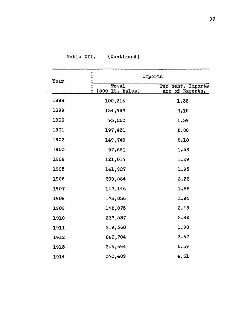
93

Table XII* (Continued.)

YearImports

: Total : (500 lb. bales)

Per oent. Imports are of Exports.

1898 100,316 1.321899 134,797 2.151900 93,263 1.391901 197,431 2.801902 149,749 2.101903 97,681 1.581904 121,017 1.391905 141,927 1.951906 209,584 2.321907 142,146 1.861908 173,036 1.941909 172,075 2.681910 227,537 2.821911 219,560 1.981912 243,704 2.671913 246,694 2.591914 370,409 4.31

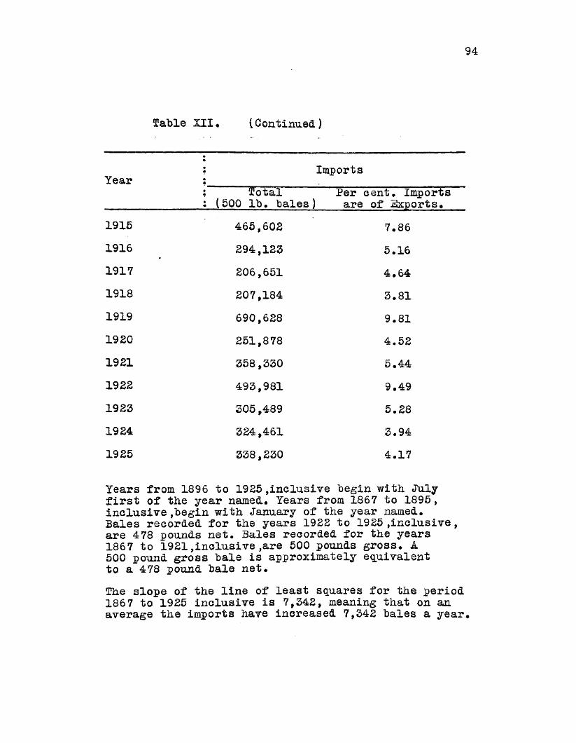
94

Table XII. (Continued)

Year Imports? Total : (500 lb. bales)

Per cent. Imports are of Exports.

1915 465,602 7.861916 294,123 5.161917 206,651 4 . 641918 207,184 3.811919 690,628 9.811920 251,878 4.521921 358,330 5.441922 493,981 9.491923 305,489 5.281924 324,461 3.941925 338,230 4.17

Years from 1896 to 19£5,inclusive begin with July first of the year named. Years from 1867 to 1895, inclusive,begin with January of the year named.Bales recorded for the years 1922 to 1925 inclusive, are 478 pounds net. Bales recorded for the years 1867 to 1921,inclusive,are 500 pounds gross. A 500 pound gross bale is approximately equivalent to a 478 pound bale net.The slope of the line of least squares for the period 1867 to 1925 inclusive is 7,342, meaning that on an average the imports have increased 7,342 bales a year.

95

Table XIII. Origin of Cotton Imported into the United States, 1919-26*

Country from which imported

Per cent, of Cotal Imports1919 1920 1921 1922

British India 2.8 2.3 1.4 4.1%ypt 49.3 60.0 52.5 34.6Mexico 17.6 12.7 28.2 35.0Peru 11.5 8.5 9.3 9.0United Kingdom 10.6 4.7 5.1 5.2China (1) 9.2Other Countries 8.2 11.8 3.5 2.9

Total 100.0 100.0 100.0 100.0

*Yearboo& of the U. S.P.A., 1922, page 979, Table 522,1923, page 1130a /t QQ , Table 660 , and 1926, page 1194,

(1) Accurate statistics for China not available prior to 1922.

96

(Fable XIII* (Continued)

Country from which imported

••: Per••

Cent, of (Total Imports (1):1923 1924 1925 1926

British India 2.9 11.2 8.4 6.9Egypt 61.9 53.8 59.3 69.7Mexico 15.0 9.2 14.4 7.3Peru 9.7 6.8 3.6 4.6United Kingdom 3.1 (2) (2) (2)China 4.3 H • 00 10.3 7.9Other Countries 3.1 4.2 4.0 3.6

(Total 100.0 100.0 100.0 100.0

(1) Year ending June 30th. Data for 1919, 1920, and .1921 are for year ending December 31st.

(2) Accurate statistics for United Kingdom not .available.

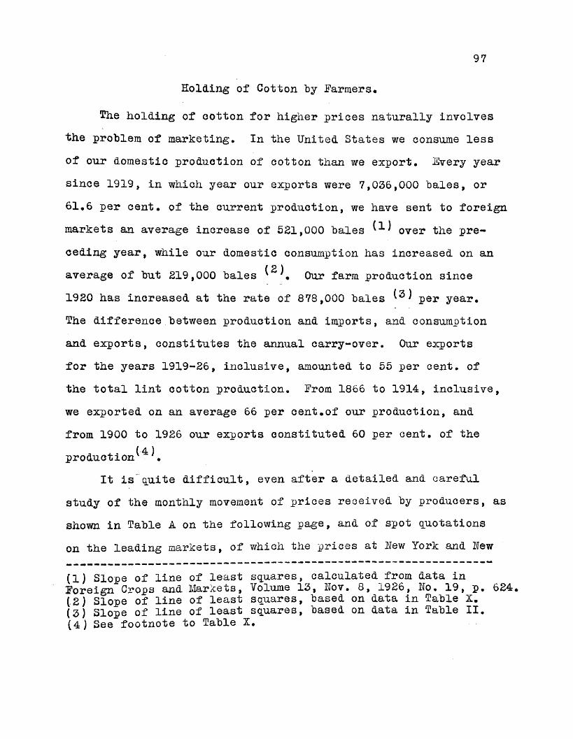
97

Holding of Cotton by Farmers*

The holding of eotton for higher prices naturally involves the problem of marketing* In the United States we consume less of our domestic production of cotton than we export. Fvery year since 1919, in which year our exports were 7,036,000 bales, or 61.6 per cent, of the current production, we have sent to foreign markets an average increase of 521,000 bales over the pre­ceding year, while our domestic consumption has increased on an average of but 219,000 bales ^^* Our farm production since 1920 has increased at the rate of 878,000 bales per year.The difference between production and imports, and consumption and exports, constitutes the annual carry-over. Our exports for the years 1919-26, inclusive, amounted to 55 per cent, of the total lint cotton production. From 1866 to 1914, inclusive, we exported on an average 66 per cent*of our production, andfrom 1900 to 1926 our exports constituted 60 per cent, of the

(4 )production' ♦It is quite difficult, even after a detailed and careful

study of the monthly movement of prices received by producers, as shown in Table A on the following page, and of spot quotations on the leading markets, of which the prices at Hew York and Few

(1) Slope of line of least squares, calculated from data inForeign Crops and Markets, Volume 13, Nov. 8, 1926, No. 19, p. 624*(2) Slope of line of least squares, based on data in Table X.(3) Slope of line of least squares, based on data in Table II.(4) See footnote to Table X.

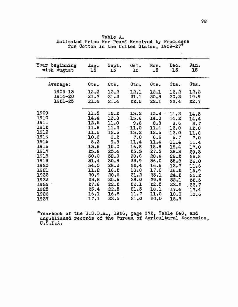
98

Table A.Estimated Price Per Pound Received by Producers

for Cotton in the United States, 1909-27

‘ beginning th August Aug*

15Sept.15

Oct.15

Rov.15

Dec.15

Jan.15

Average: Cts* Cts* Cts. Cts. Cts. Cts.1909-13 12.3 12.2 12.1 12.1 12.2 12.21914-20 21.7 21.2 21.1 20.8 20.2 19.91921-25 21*4 21.4 22.5 22.1 22.4 22.7

1909 11.5 12.2 13.2 13.8 14 . 2 14.31910 14.4 13.8 13.6 14 . 0 14.2 14.41911 12.5 11.0 9.6 8.8 8.6 8.71912 11.6 11.2 11.0 11.4 12.0 12.01913 11.6 12.6 13.2 12.6 12.0 11.81914 10.6 8.2 7.0 6.6 6.7 7.01915 8.3 9.8 11.4 11.4 11.4 11.41916 13.6 15.0 16.8 18.8 18.4 17.01917 23.8 23.4 25.3 27.5 28.3 29.31918 30.0 32.0 30.6 28.4 28.2 26.81919 31.4 30.8 33.9 36.0 35.8 36.01920 34.0 28.3 22.4 16.6 12.7 11.61921 11.2 16.2 18.8 17.0 16.2 15.91922 20.9 20.6 21.2 23.1 24.2 25.21923 23.8 25.6 28.0 29.9 32.1 32.51924 27.8 22.2 23.1 22.5 22.2 . 22.71925 23.4 22.5 21.5 18.1 17.4 17.41926 16.1 16.8 11.7 11.0 10.0 10.61927 17.1 22.5 21.0 20.0 18.7

’‘‘Yearbook of the U.S.D.A., 1926, page 972, Table 248, and unpublished records of the Bureau of Agricultural Economies, U.S.D.A.

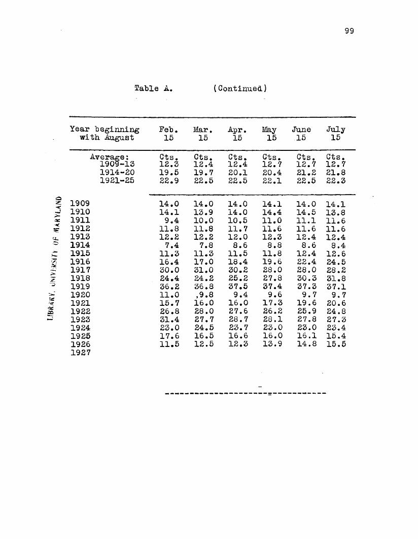
W. <-MVi k

Slf, O

f

99

Table A. (Continued)

Year beginning with August Feb.

15Mar.15

Apr.15

May15

June15

July15

Average: Cts. Cts. Cts. Cts. Cts. Cts.1909-13 12.3 12.4 12.4 12.7 12.7 12.71914-20 19.5 19.7 20.1 20.4 21.2 21.81931-25 22.9 22.5 22.5 22.1 2 2.5 22.3

1909 14.0 14.0 14.0 14.1 14.0 14.11910 14.1 13.9 14.0 14.4 14.5 13.81911 9.4 10.0 10.5 11.0 11.1 11.61912 11.8 11.8 11.7 11.6 11.6 11.61913 12.2 12.2 12.0 12.3 12.4 12.41914 7.4 7.8 8.6 8.8 8.6 8.41915 11.3 11.3 11.5 11.8 12.4 12.61916 16.4 17.0 18.4 19.6 22.4 24.51917 30.0 31.0 30.2 28.0 28.0 28.21918 24.4 24.2 25.2 27.8 30.3 31.81919 36.2 36.8 37.5 37.4 37.3 37.11920 11.0 ,9.8 9.4 9.6 9.7 9.71921 15.7 16.0 16.0 17.3 19.6 20.61922 26.8 28.0 27.6 26.2 25.9 24.81923 31.4 27.7 28.7 28.1 27.8 27.31924 23.0 24.5 23.7 23.0 23.0 23.41925 17.6 16.5 16.6 16.0 16.1 15.41926 11.5 12.5 12.3 13.9 14.8 15.51927

100

Orleans as shown in Table XIV are typical, to reach a satis­factory conclusion regarding the extent to which the storing and holding of cotton on farms and in warehouses is a paying venture under present economic conditions* Since 1920, increases in spot quotations on the New York Market for cotton sold in April have been as high as 48 per cent, over the preceding year, and decreases have been as great as 71 per cent/V In Table A are shown the prices received by producers as reported for the fifteenth of each month* These prices on an average show very little change from October to May. In general, the prices paid to producers increase after October in years of a short crop, and tend to decrease in years when there is a heavy crop. The writer, of course, is mindful of the fact that the prices reported by the United States Department of Agriculture for the fifteenth of each month are not entirely satisfactory for the basis of specific conclusions, but they adequately serve the purpose for which we wish to use them.

On the following page, Table B, are shown the percentages of monthly marketings by farmers. As will be seen, by the end of November for the years 1912-26, inclusive, the per cent, of the cotton crop that had passed from the hands of the producers into the channels of the cotton trade ranged from 45 in 1920 to 70 in 1923. The per cent, of current production that is marketed by the end of Hovember does not vary directly in proportion to the size

(1)See Table XIV.

101

Table B*Estimated Monthly Marketings of Cotton

by Farmers, 1912-25*

Year beginning August 1st* Percentage of year’s sales

: Aug. Sept. Oct. Nov. Dec. Jan.1912-13 .... 17.2 25.8 20.3 12.8 8.01913-14 .... 18.2 24.4 19.7 13.3 8.31914-15 1.2 6.8 14.8 18.0 16.1 11.01915-16 2.7 11.3 19.3 20.4 16.4 8.41916-17 3.9 14.6 23.0 21.6 15.0 6.41917-18 2.5 11.3 23.0 22.7 16.2 8.21918-19 3.3 10.9 18.1 16.4 13.6 5.41919-20 1.4 9.5 21.0 22.2 17.4 8.81920-21 3.1 10.0 16.2 15.7 11.0 6.41921-22 3.6 14.0 22.3 17.1 12.1 5.91922-23 5.2 16.8 25.3 19.8 12.8 5.91923-24 4.1 16.3 24.6 24.9 13.3 5.81924-25 3.3 15.2 25.2 22.3 14.5 7.01925-26 6.5 19.3 23.1 17.6 12.0 6.5

*Yearbook of the U.S.D.A., 1923, page 805, Table 302, and 1926, page 970, Table 246.On an average, about 13 per cent, of the cotton crop is marketed by farmers in September, 21 per cent, in October, 19 per cent, in November, and 14 per cent, in December.The data in Tables IV and XIV, showing production and spot prices, and the prices received by producers, as reported in Table A,(preceding page), all seem to indicate that there is a stronger tendency for prices to fluctuate in accordance with the size of the crop than with the quantity of cotton actually offered on the market during any one month. Unwarranted holdings by producers would ultimately tend to encourage importation by American manufacturers. The more immediate results would be the stimulation of foreign production and the restriction of foreign markets for American cotton.

102

Table B. (Continued)

Estimated Monthly Marketings of Cotton "by Farmers, 1912-25.

♦Year * Percentage of year*s sales__________ ; Feb. Mar. 'Apr. May June July Season1912-13 5.2 4.5 2.61913-14 5.3 4.4 2.71914-15 8.3 7.7 6.11915-16 5.4 5.2 3.91916-17 4.0 3.9 3.01917-18 5.8 4.5 2.61918-19 4.4 4*6 4.61919-20 5.6 4.9 3.21920-21 5.6 6.0 6.71921-22 4.3 4.6 4.61922-23 4.4 3.7 2.01923-24 3.1 2.4 1.71924-25 5.3 3.4 1.61925-26 4.2 3.1 2.3

1.5 1.1 1#0M \ 1001.5 1.2_ 1002.5 7.5}* ... 1003.6 3.4(2)... 1002.5 1.6 .5 1001.3 1.0 .9 1007.5 6.8 4.4 1002.7 1.7 1.6 1006.9 6.8 5.6 1005.9 3.0 2.6 1001.0 1.5 1.6 1001.3 .9 1.6 1001.0 .6 .6 1001.7 2.1 1.6 100

(1) Includes August(2) Includes July.

103

of the crop, nor Inversely, as to that matter, since stocks on hand at the beginning of the season constitute an influencing factor. In 1921 the current production was 7,954,000 bales, the smallest crop since 1895. Ordinarily, an increase in the per­centages of monthly marketings would have been expected during the first few months of the season, but, as shown in Table C, the stocks on hand amounted to 6,590,000 bales, which were equiva­lent to about 83 per cent, of the current production.

It must not be concluded that the producer acts as a bear on his own market. There is,undoubtedly, some relation between the quantity of cotton marketed in early fall and the prices received, but this relationship is not so marked as is sometimes thought, except that quantity marketed at harvest time may have some relation to aggregate supply, including both production and carry-over. Cotton prices depend largely upon the size of the crop, rather than upon the time the crop is marketed. In Charts A and B are plotted the prices of cotton and cotton stocks arriving for sale at hew Orleans for the seasons of 1921-22 and 1922-23. There is, the reader will observe, no relation between the movements of the curves representing the two factors. An increase in receipts is equally likely to be accompanied by either a rise or fall in prices. In Table D the analysis is continued, and there will be seen the expressions of relationship between prices and stocks at the hew Orleans Market, There seems

104

Table C.Stocks on Hand, Aggregate Supply, and Consumption of Cotton in the United

States, 1905— 25*

Year Stocks on Aggregate Consumption(1) hand at supply

beginning of year (2)

(3)

11,000 bales 1,000 bales 1,000 bales1905 1,935 12,794 4,9091906 1,349 14,857 4,9851907 1,515 12,982 4,5391908 1,236 14,833 5,2411909 1,484 12,021 4,7991910 1,040 13,237 4,7051911 1,375 17,713 5,3681912 1,777 16,093 5,7861913 1,511 15,760 5,5771914 1,366 17,636 5,5971915 3,936 15,425 6,3981916 3,140 14,792 6,7891917 2,720 14,185 6,5661918 3,450 15,553 5,7661919 4,287 16,295 6,4201920 3,563 17,045 4,8931921 6,590 14,920 5,9101922 2,832 13,011 6,6661923 2,325 12,768 5,6811924 1,556 15,638 6,1931925 1,610 17,934 6,451foreign Crops and Markets, Volume 13, Hov. 8,1926, Humber 19, page 624*(1)Year beginning with August*(2)Includes foreign cotton.(3)Includes stocks on hand, ginnings, and imports.

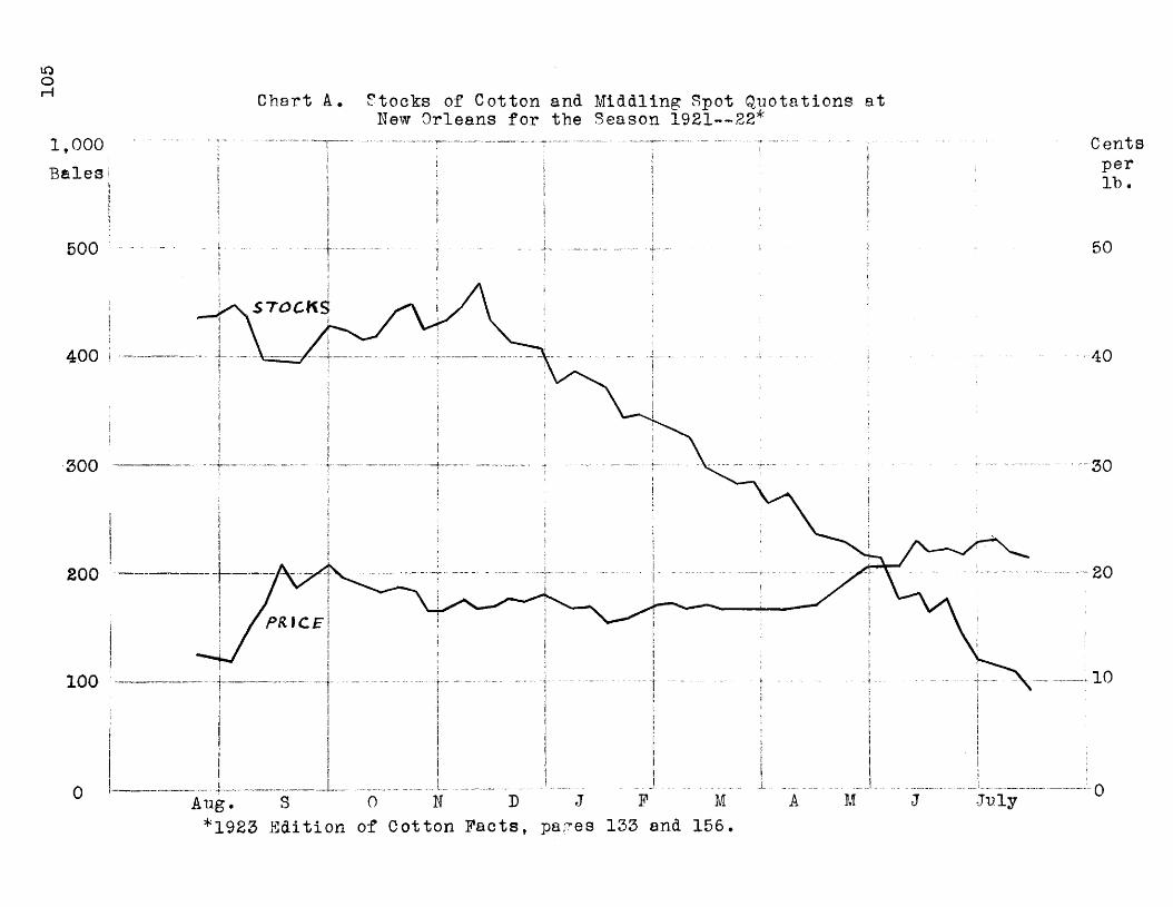
105

Chart A. Stocks of Cotton and Middling Spot Quotations at New Orleans for the Season 1921— 22*

CentsperIh.

1,000Bales

50500

STOCKS

400 40

300 30

20200

10100

1923 Edition of Cotton Facts, pares 133 and 156.

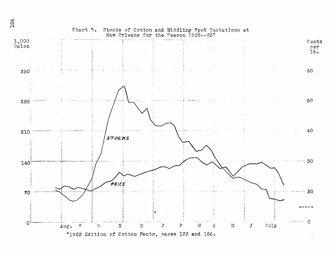
oI— I

1,000Bales

Chart 3. Stocks of Cotton and Middling Spot Quotations at New Orleans for the Season 1922— 23*

Centsperlh.

350 60

280

210

140

70

_!

*1923 Edition of Cotton Pacts, pages 133 and 156*

50

40

30

20

0

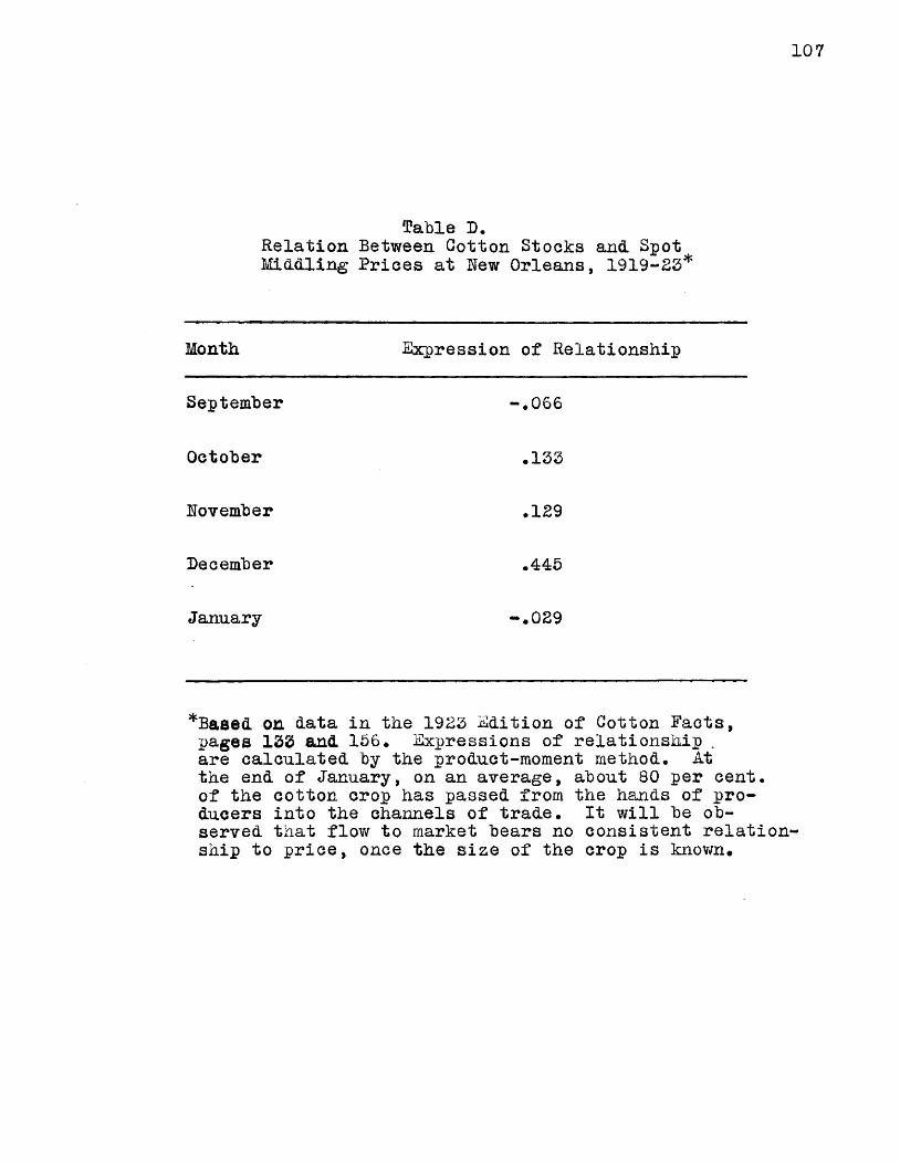
107

3?able D.Relation Between Cotton Stocks and Spot t Middling Prices at New Orleans, 1919-23*

Month Expression of Relationship

September -.066

October .133

November .129

December .445

January -.029

*Based on data in the 1923 Edition of Cotton Pacts, pages 133 and 156• Expressions of relationship are calculated by the product-moment method. At the end of January, on an average, about 80 per cent, of the cotton crop has passed from the hands of pro­ducers into the channels of trade. It will be ob­served that flow to market bears no consistent relation­ship to price, once the size of the crop is known*

108

to be no consistency in the movements of prices in relation to market receipts, which indicates their fluctuations are due to factors other than mere quantity of cotton received for sale at any particular time. In 1919 and 1921 the cotton crop declined620.000 and 5,486,000 bales in relation to the respective pre­ceding years, and in each case there was an upward trend in prices during the season. In 1920 there was an increase of2.019.000 bales over 1919, and there followed a sharp decline in prices after September. The largest cotton crop the United States has ever produced was in 1926, when the ginnings totaled17.977.000 bales. During this season the prices declined very sharply, and they continued to decline until the probable short crop of 1927 became evident, after which there was a tendency upward. These facts point to the rather definite conclusion that cotton prices fluctuate inversely with the size of the cotton crop, rather than with the rate of flow to market. This same relationship applies to all the large cotton exchanges in the country, though in different degrees. New Orleans, for example, is an interior spot market located near the great cotton- producing centers, and there is often less of the speculative element involved in the prices here than at New York, which is primarily a futures market.

According to the quotations in Table A the increases in prices to producers in May over the preceding October have ranged

109

from .1 of a cent a pound in 1923 to 5 cents in 1922, while decreases in May prices as compared with preceding October prices were as great as 12.8 cents in 1920, and as low as .1 of a cent in 1924.' During the eighteen year period, 1909— 26, prices in twelve years were higher in May than in October, and in six years they were lower. Omitting the war period, there were only eight years in which the May prices were higher than October prices. The United States Department of Agriculture has made studies of the cost of storing cotton, but these show average costs, and are, therefore, of little assistance to the individual producer in aiding him to decide upon the advisability of holding his crop off the market. In short-crop years,the prediction that prices will rise and continue to rise after October may be relied upon as unmistakably as any other economic fact, and in years of a heavy crop the price is just as surely to fall. These are two of the factors which will aid the pro­ducers and cooperative associations in arriving at a decision regarding the profitableness of holding. Another is the cost under the particular conditions, and this must be decided by each individual.

The holding of cotton for higher prices when the prices offered are sufficiently high in relation to supply and demand to allow a fair profit is not altogether economically sound, and it has often been indefensible. Any general movement to excess­

110

ively increase domestic prices will ultimately lead to disaster. Under such condition the production of cotton in foreign countries would be stimulated, resulting in a restriction of markets for American cotton. This would in turn result in a still further depression of prices, since from three-fifths to two-thirds of our production is exported. Hence, an unwarranted holding of cotton, if it were to become widespread and general, would result in greater production in foreign countries, which would become our competitors for world markets, and there would be fewer buyers for our own cotton. A persistency in the movement would ultimately tend to encourage importation by American manufacturers.

Since most of the lint cotton produced in the United States passes into the world’s channels of trade, and since, as stated, holding of eotton would be followed by a tendency for other countries to increase their production, and eventually defeat the purpose for which the holdings were made, no excessive gains are to be expected from such practices that are not wholly in harmony with the law of supply and demand. We know, of course, that supply and demand react upon prices for short periods, and that the cost of production is the main regulator of prices over a long period. The price regime involves also the concept that the cost of production determines to a large extent the prices of the future, and that costs of the past cannot become the regulator of present priees.

Ill

Cotton Markets

A ootton market is a place wiiere two or more people meet to buy and. sell cotton* The system of marketing begins in the small towns and. at the country stores, where the cotton producers and the cotton dealers meet. The marketing function, so far as lint cotton is concerned, ends when the dealer makes his delivery to the spinner. Transactions in cotton trading are carried on by sales of actual cotton and by contracts for delivery at some future time. Actual cotton sold on the market is known in the channels of trade as "spot cotton", the market on which it is sold is known as a "spot market", and the price is referred to as a "spot quotation" or as a "spot priced

In the cotton-marketing regime there are several types of markets, and these may be classified according to location and functions in trading. First, there are the spot markets. Of these there are three kinds, the primary, the interior, and the large organized exchange. The difference between the last two named is not clearly defined in all cases. Primary markets are small towns, gins, and country stores

112

where the baled eotton is first marketed and sold by producers. At many of these primary markets there is but one buyer, who does his own sampling and grading, and bids his price accordingly. At the larger markets, however, such as Troy, Alabama, there are often several buyers, and the bidding becomes more or less competitive. In the season of 1926 the writer personally visited primary spot markets in practically all of the cotton-producing states. At certain markets in Alabama, G-eorgia, and Texas the producers were literally forced to sell their cotton on the basis of grades established by the local dealer. At one market in Texas, and at another in Arkansas, three buyers, bidding on the same cotton, were offering a maximum of six cents per pound for what they classed as low middling, which is grade number 7. Farmers were not protesting against the price so much as they were against the method of grading, since they felt that Federal sampling and classing would have assured a higher price.

Interior spot markets, also known as central markets, are large towns and cities to which cotton

113

is shipped from primary spot' markets and sold by primary buyers to mills and to merchants operating on a large scale, These markets, of which Fort Worth, Memphis, Little Rick, Columbia, St. Louis, Macon, and Shreveport are typical examples, are usually points of assembling in large quantities for sampling, grading, compressing, and consigning to centers of consumption, They provide facilities for storage and are themselves markets for the sale and resale of cotton.

Future markets are located in Lew York and Lew Orleans, and their importance is indicated, not by the cotton received, but by the trading in future contracts. Dealers and manufacturers who wish to hedge a trans­action buy their contracts on the future markets, and in this way protect themselves against a rise or fall in prices. The cotton exchange at Lew Orleans is both a spot market and a future market, while Lew York is primarily a future market. Liverpool is the most im­portant foreign market dealing in American cotton. All cotton delivered on the Lew Orleans and Lew York future exchanges is now classified by the United States Department of Agriculture.

114

The cities along the Atlantic and Gulf Coasts, such as Savannah, Galveston, and Norfolk, where cotton is sold for export, are called "export markets". More than one-half of the American cotton crop is exported for consumption in foreign mills!-*-) The leading countries to which the cotton is exported are as follows: United Kingdom, Germany, France, Italy, and Japan, faring the year ending June 30th, 1926, our total exports of lint cotton amounted to 8,109,544 bales of 500 pounds each. (See Tahle XI) Of this quantity, the United Kingdom received 28.1$, Germany 20.4$, France 11.4$, Italy 9.2$, other European countries 12.6$, Japan 13.8$, and other countries 4,5$. Linters are exported mainly to Germany.^ 2)

On all the cotton exchanges in the United States, "American Middling”, the standard short-staple grade, is the basis of price quotations for all short-staple cottons. Upland short-staple cotton constitutes about 92 per cent, of the total cotton crop of the United States and about 50 per cent, of the total worldTs erop.^)

(lJ See Table X(2J See 1926 U.S.f.A. Yearbook, page 1185, Table 498 (3J Miss F. Anderson, United States Dept, of Agri.

115

Monthly Spot Prices at New York and. Hew OrleansSpot (quotations at all the cotton exchanges are based on

Middling, which is grade 5. She differences in price between Middling and the other grades and the premiums for the longer staples vary from time to time because of special demands or the effects of seasonal weather factors upon the supply of the different grades and lengths of staple, fable XIV shows the spot prices for Middling cotton at hew York for the years 1892- 1927, inclusive, and at hew Orleans for the years 1900-27, inclusive, fhe spot prices at hew York are generally a little higher than at hew Orleans because of the cost of transportation involved in moving cotton to the former, Fluctuations in price are due largely to the size of the crop, and, as will be observed, they have been quite varied. Average monthly spot prices during the World War rose to 35.09 cents per pound at hew York in September of 1918 and to 33.22 cents at hew Orleans in the same month and year. Prices during the World War period, however, were not as high as in the Civil War period, one reason beingthat production continued and there was always a good supplyavailable, whereas in the earlier period very little cotton was produced, and almost none was available.

In the season of 1919-20 spot prices reached the highest level since the Civil War, surpassing by far the prices of any one year of the World War. In the latter part of the 1920-21 season prices declined to the pre-war level, but rose again in1921-22, and continued at a high level until the fall of 1926,when they again receded to near the pre-war level.

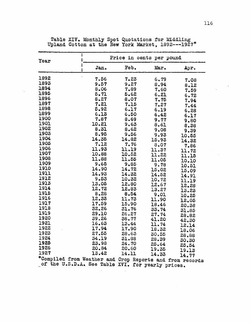
116

Table XIV, Monthly Spot Quotations for Middling Upland Cotton at the Uew York Market, 1892---1927*

Year Price in cents per poundJan, Feb, Mar, Apr.

189218931894189518961897189818991900190119021903190419051906190719081909191019111912191319141915191619171918191919201921192219231924192519261927

7.56 7.23 6.79 7.089,57 9.27 8.94 8.128,06 7.89 7.60 7.595.71 5.62 6.21 6.728.27 8.07 7.75 7.947.21 7.15 7.27 7.445.92 6.17 6.19 6.286.13 6.50 6.42 6.177,87 8.69 9.77 9.8010.21 9.63 8.61 8.388.31 8.62 9.08 9.398.95 9.56 9.93 10.5514.35 14.82 15.93 14.327.12 7.76 8.07 7.8611.93 11.19 11.37 11.7210.88 10.52 11.22 11.1511.88 11.55 11.05 10.109.65 9.85 9.78 10.5114.90 14.72 15.02 15.0914.93 14.32 14.52 14.919.53 10.32 10.72 11.1913.05 12.80 12.67 12.2812.72 12.83 13.27 13.238.28 8.54 9.01 10.2512.33 11.73 11.90 12.0517.59 15.90 18.46 20.3832.26 31.76 33.74 31.8529.10 26.27 27.74 28.8239.26 38.77 41.20 42.3016.63 13.44 11.74 12.1417.94 17.90 18.32 18.0627.55 28.63 30.55 28.8834.19 31.88 28.39 30.3023.98 24.70 25.64 25.5420.8413.42

20.6014.11 19.35

14.33 19.1314.77

- - - - - - - - - - - - - - - - - - - - - - - - - - - - - - - - - - - - - - - - w n &U.J.V4. i '

of the U.S .D.A, See Table XVI, for yearly prices.

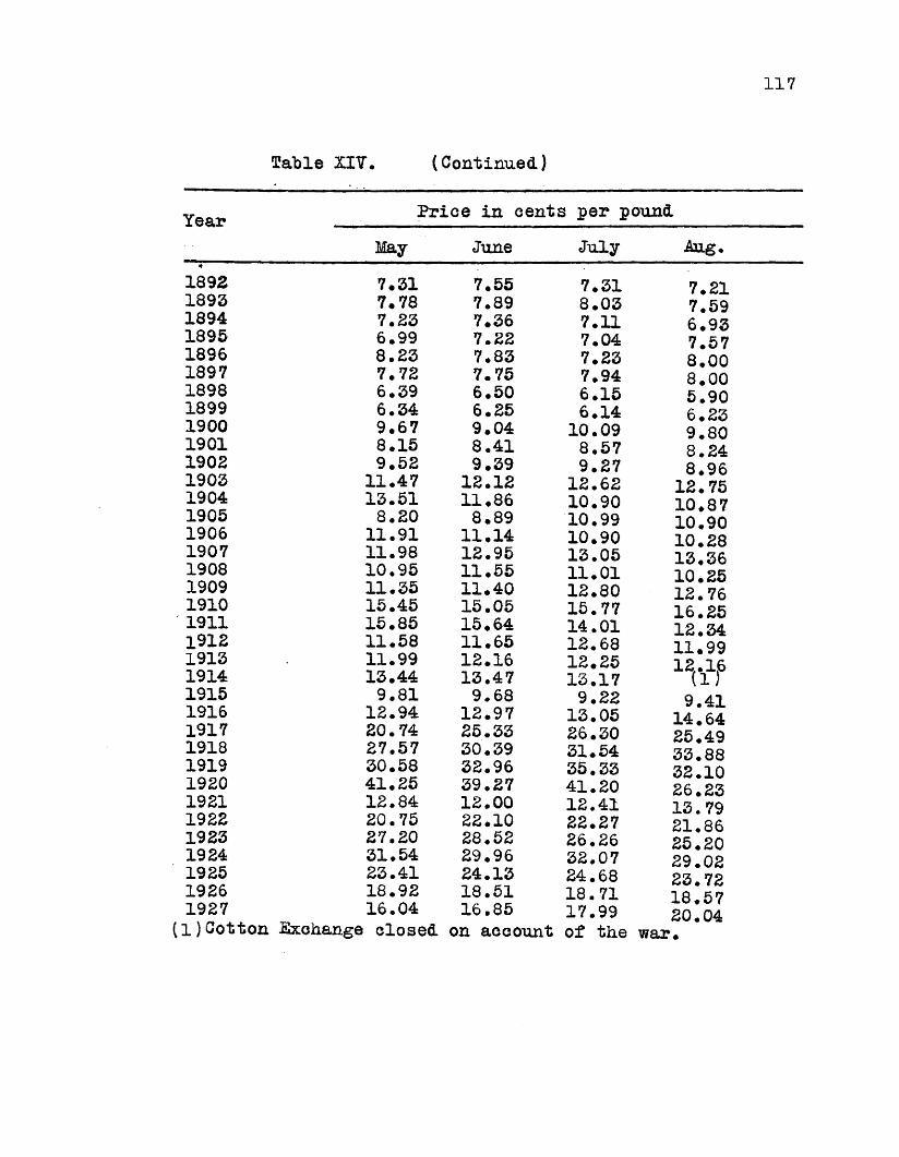
117

Table ZI7. (Continued)

Price in cents per poundMay June July Aug.

41892 7.31 7.55 7.31 7.211893 7.78 7.89 8.03 7.591894 7.23 7.36 7.11 6.931895 6.99 7.22 7.04 7.571896 8.23 7.83 7.23 8.001897 7.72 7.75 7.94 8.001898 6.39 6.50 6.15 5.901899 6.34 6.25 6.14 6.231900 9.67 9.04 10.09 9.801901 8.15 8.41 8.57 8.241902 9.52 9.39 9.27 8.961903 11.47 12.12 12.62 12.7519041905 13.51

8.2011.868.89 10.90

10.99 10.8710.901906

19071908

11.9111.9810.95

11.1412.9511.55

10.9013.0511.01

10.2813.3610.251909

19101911

11.3515.4515.85

11.4015.0515.64

12.8015.7714.01

12.76 16.25 12.341912 11.58 11.65 12.68 11.991913 11.99 12.16 12.25 12.161914 13.44 13.47 13.17 (1 )1915 9.81 9.68 9.22 9.411916 12.94 12.97 13.05 14.641917 20.74 25.33 26.30 25.491918 27.57 30.39 31.54 33.881919 30.58 32.96 35.33 32.101920 41.25 39.27 41.20 26.231921 12.84 12.00 12.41 13. 791922 20.75 22.10 22.27 21.861923 27.20 28.52 26 • 26 25.201924 31.54 29.96 32.07 29.021925 23.41 24.13 24.68 23.721926

192718.9216.04

18.5116.85 18.71

17.99 18.5720.04(1 ) Cotton Exchange closed on account of the war.

118

Table XIV. (Continued)

Year Price in cents per poundSept* Oct. Hov. Pec

1892 7*33 8*09 9*24 9 771893 8.19 8.33 8.17 7*91

5.72 8.36

1884 6.74 6*04 5.761895 7.41 9.00 8.66

1906 8.76 11.11 10.801907 12.54 11.55 n.801908 9.38 9.18 9.391909 13.29 13.90 14.701910 13.89 14.44 14.781911 11.28 9.65 9.421912 11.81 11.10 12.361913 13.46 14.05 13.701914 (1) (1) (2)1915 10.83 12.37 11.89

8.6213.017.69

1896 8.54 8.00 7.89 7 211897 7.08 6.33 5.88 5 .$%1898 5.62 5.42 5.40 5 701899 6.60 7.31 7.62 7*661900 10.53 10.16 9.80 10*191901 8.39 8.42 7.95 8*471902 8.94 8.80 8.051903 11.84 9.70 11.181904 10.92 10.36 9.911905 10.84 10.39 11.49 1 2 !15

lo! 65 11.96 9.24

15.30 15.079.46

13.04 12.99 7.53

i ? * ? ? 1 9 - 9 2 18*2930.74 30.22 39.1915.6818.30 25.65 35.92 23.85 20.0612.68 19.58

1917 23.05 28.02 29.781918 35.09 32.42 29.691919 30.60 34.98 39.401920 30.07 22.68 18.811921 19.95 19.63 18.011922 21.35 22.73 25.641923 29.06 30.06 34.731924 24.24 24.51 24.221925 23.79 21.77 20.941926 17.01 13.14 12.861927 21.93 20.96 20.22(1 ) Cotton Exchange closed, on account of the war"(2 )Cotton Exchange closed until November 16th.

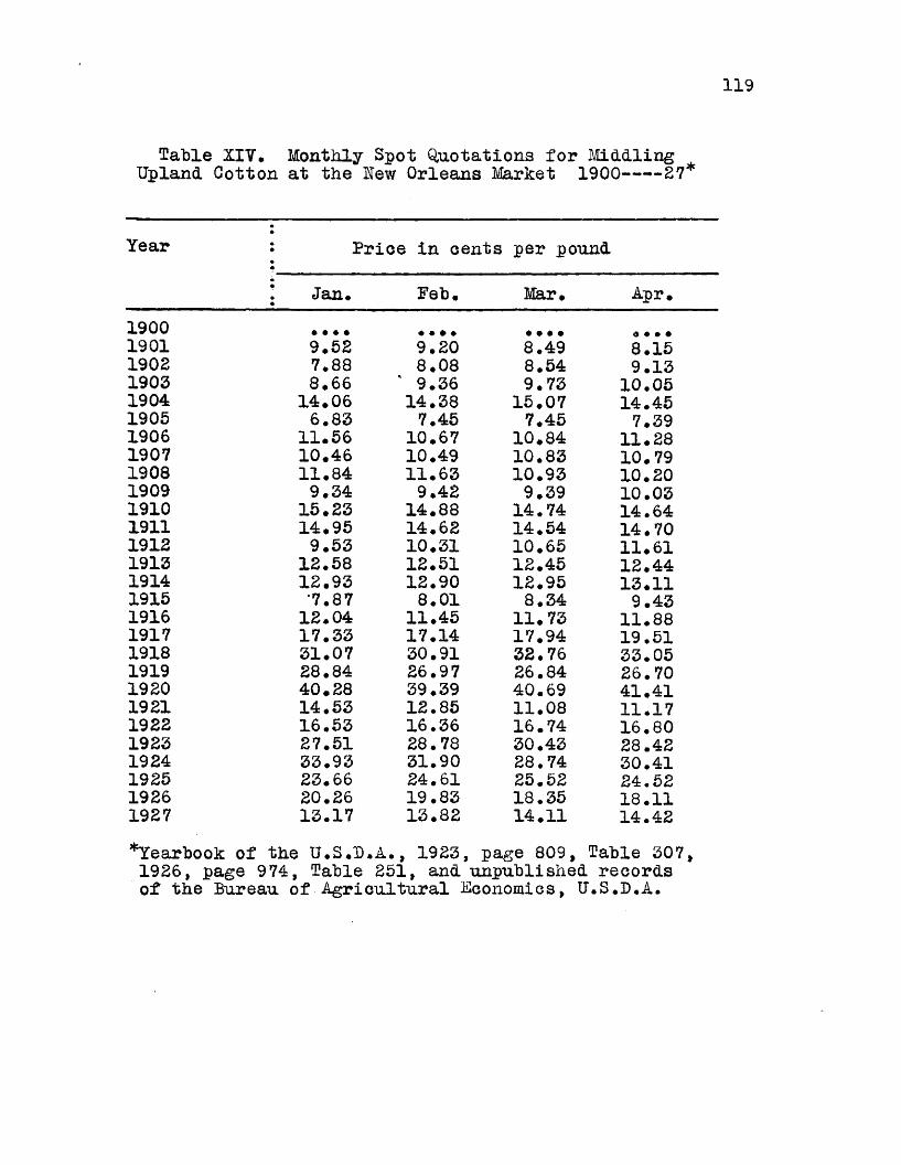
119

Table XIV. Monthly Spot Quotations for Middling Upland Cotton at the New Orleans Market 1900— --£7*

Year • Price in cents per pound

♦ Jan. Feb. Mar. Apr.1900 • • • • * . . . •. •. ....1901 9*52 9.20 8.49 8.151902 7.88 8.08 8.54 9.131903 8.66 ' 9.36 9.73 10.051904 14.06 14.38 15.07 14.451905 6.83 7.45 7.45 7.391906 11.56 10.67 10.84 11.281907 10.46 10.49 10.83 10.791908 11.84 11.63 10.93 10.201909 9.34 9.42 9.39 10.031910 15.23 14.88 14.74 14.641911 14.95 14.62 14.54 14.701912 9.53 10.31 10.65 11.611913 12.58 12.51 12.45 12.441914 12.93 12.90 12.95 13.111915 7.87 8.01 8.34 9.431916 12.04 11.45 11.73 11.881917 17.33 17.14 17.94 19.511918 31.07 30.91 32.76 33.051919 28.84 26.97 26.84 26.701920 40.28 39.39 40.69 41.411921 14.53 12.85 11.08 11.171922 16.53 16.36 16.74 16.801923 27.51 28.78 30.43 28.421924 33.93 31.90 28.74 30.411925 23.66 24.61 25.52 24.521926 20.26 19.83 18.35 18.111927 13.17 13.82 14.11 14.42*Yearbook of the U.3.D.A., 1923, page 809, Table 307, 1926, page 974, Table 251, and unpublished records of the Bureau of Agricultural Economies, U.S.D.A.

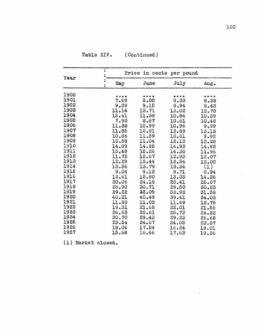
120

Tatle XIV. (Continued)

Price in cents per poundYear! May June July Aug.

1900 # # ♦ * .... .... • * • •1901 7.69 8.05 8.33 8.281902 9.39 9.15 8.94 8.431903 11.14 12.71 13.02 12.701904 13.41 11.38 10.86 10.591905 7.90 8.87 10.61 10.481906 11.33 10.99 10.96 9.991907 11.85 12.81 12.89 13.131908 10.86 11.59 10.81 9.921909 10.59 11.04 12.13 12.281910 14.89 14.85 14.93 14.921911 15.48 15.26 14.30 11.961912 11.72 12.07 12.93 12.071913 12.29 12.44 12.34 12.021914 13.36 13.79 13.34 (1 )1915 9.04 9.12 8.71 8.941916 12.61 12.80 13.03 14.261917 20.06 24.18 25.41 25.071918 28.90 30.71 29.50 30.231919 29.22 32.09 33.93 31.381920 40.31 40.49 39.41 34 .031921 11.80 11.03 11.49 12.781922 19.31 21.68 22.01 21.551923 26.63 28.61 25.73 24.221924 30.70 29.43 29.23 26.651925 23.54 24.07 24.05 23.071926 18.06 17.54 18.24 18.011927 15.68 16.46 17.63 19.36(1 ) Market closed.

121

Table XIV. (Continued)

Price In cents per poundI Sept. Oct* Nov. Dec.

1900 10.39 9.57 9.48 9.501901 8.15 7.99 7.32 7.931902 8.43 8.22 7.82 8.141903 10.72 9.66 10.72 12.521904 10.54 9.80 9.50 7.481905 10.26 10.16 11.28 11.881906 9.24 10.76 10.39 10.531907 12.41 11.19 10.84 11.541908 9.11 8.92 8.97 8.781909 12.66 13.48 14.40 14.961910 13.49 14.21 14.50 14.851911 11.29 9.61 9.35 9.171912 11.37 10.95 12.15 12.811913 13.11 13.73 13.26 12.981914 (2) 8.42 7.02 7.43 7.181915 10.40 11.95 11.50 11.891916 15.27 17.24 19.45 18.341917 21.68 26.76 28.07 29.071918 33.22 31.18 29.75 29.441919 30.38 35.28 39.58 39.891920 27.48 20.95 17.65 14.591921 19.35 18.99 17.27 17.161922 20.74 22.05 25.34 25.48.1923 27.71 29.18 33.68 34.881924 22.79 23.48 23.95 23.661925 23.09 20.86 19.82 19.271926 16.14 12.68 12.52 12.221927 21.53 20.73 19.99 19.26(2 ) No quotations prior to Sept. 23• Average for

122

Secular Trend of Prices

With the exception of the World War period, and the years immediately following, cotton prices have risen grad­ually one year over another since 1866, and particularly since 1892. This tendency toward a uniform upward trend may he attributed mainly to the increased volume of money in circulation, which hears approximately the same ratio to pro­duction as production bears to demand for cotton.

Table XV shows the calculated ordinates of monthly trend of spot prices at Hew York for the period 1892-1912, inclusive. Ihiring these years the average of monthly prices was never above 10.0 cents nor below 9.0 cents. The lowest average of 9.39 cents was for the month of October, and the highest average of 9.97 cents was for July, constituting a difference of .58 cents.

Charts III to XIV show graphically the actual trend of monthly prices. Particular attention is called to the closeness of fit of the least squares line. The exact determination of the nature and extent of price movements is the first and most important procedure in the analysis of causal relatiosnhips between production and price.

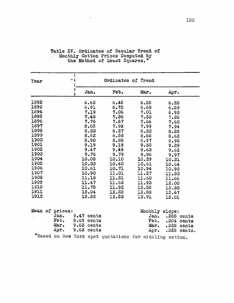
123

Table XV. Ordinates of Secular Trend of Monthly Cotton Prices Computed by

the Method of Least.Squares.*

Year«•

•Ordinates of Trend

♦• Jan.•Feb. Mar. Apr.

1892 6.62 6.45 6.35 6.251893 6.91 6.75 6.68 6.591894 7.19 7.06 7.01 6.931895 7.48 7.36 7.33 7.261896 7.76 7.67 7.66 7.601897 8.05 7.98 7.99 7.941898 8.33 8.27 8.32 8.281899 8.62 8.58 8.65 8.621900 8.90 8.88 8.97 8.951901 9.19 9.19 9.30 9.291902 9.47 9.49 9.63 9.631903 9.76 9.79 9.96 9.971904 10.05 10.10 10.29 10.311905 10.33 10.40 10.61 10.641906 10.61 10.71 10.94 10.981907 10.90 11.01 11.27 11.321908 11.18 11.31 11.60 11.661909 11.47 11.62 11.93 12.001910 11.75 11.92 12.25 12.331911 12.04 12.23 12.58 12.671912 12.32 12.53 12.91 13.01

Mean of prices: Monthly slope:Jan. ,9.47 cents Jan. .285,centsFeb. 9.49 cents Feb. .304 centsMar. 9.63 cents Mar. .328 centsApr. 9.63 cents Apr. .328 cents.

*Based on New York spot quotations for middling cotton.

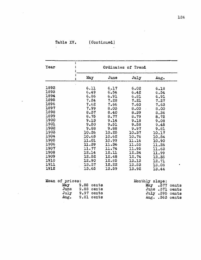
124

Table XV* (Continued)

Year Ordinates of Trend

I May June July Aug.

1892 6.11 6.17 6.02 6.181893 6.49 6.54 6.42 6.541894 6.86 6.91 6.81 6.911895 7.24 7.28 7.21 7.271896 7.62 7.66 7.60 7.631897 7.99 8.03 8.00 8.001898 8.37 8.40 8.39 8.361899 8.75 8.77 8.79 8.721900 9.13 9.14 9.18 9.081901 9.50 9.51 9.58 9.451902 9.88 9.88 9.97 9.811903 10.26 10.25 10.37 10.171904 10.63 10.62 10.76 10.541905 11.01 10.99 11.16 10.901906 11.39 11.36 11.55 11.261907 11.77 11.74 11.95 11.631908 12.14 12.11 12.34 11.991909 12.52 12.48 12.74 12.351910 12.90 12.85 13.13 12.711911 13.27 12.22 13.53 13.081912 13.65 13.59 13.92 13.44

Mean of prices:May 9.88 centsJune 9.88 centsJuly 9*9 7 centsAug. 9.81 cents

Monthly slope:May .377 cents June *37i cents July .395 cents Aug. .363 cents

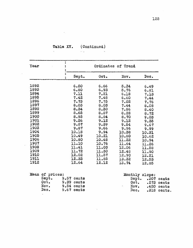
Cable XV. (Continued)

Year Ordinates of frend

Sept. Oct. Nov. Dec.

1892 6.50 6.66 5.34 6.491893 6.80 6.93 5.76 6.811894 7.11 7.21 6.18 7.131895 7.42 7.48 6 • 60 7.441896 7.73 7.75 7.02 7.761897 8.03 8.03 7.44 8.081898 8.34 8.30 7.86 8.401899 8.65 8.57 8.28 8.721900 8.95 8.84 8.70 9.031901 9.26 9.12 9.12 9.351902 9.57 9.39 9.54 9.671903 9.87 9.66 9.96 9.991904 10.18 9.94 10.38 10.311905 10.49 10.21 10.80 10.621906 10.80 10.48 11.22 10.941907 11.10 10.76 11.64 11.261908 11.41 11.03 12.06 11.581909 11.72 11.30 12.48 11.901910 12.02 11.57 12.90 12.211911 12.33 11.85 13.32 12.531912 12.64 12.12 13.74 12.85

of prices: Monthly slope:Sept. 9.57 cents Sept. .307 centsOct. 9.39 cents Oct. .273 centsNov. 9.54 cents No t . .420 centsDec. 9.67 cents Dec. .318 cents

Production

in Millions

of Ba

les

Cfhart II. Straight Line Trend of Cotton Productionin the United States, 1894— 1912*

15

13

11

Yearly Production Line of Trend

18981894 1896'Computed by the method of least squares

1900 1902 1904 1906 1908 1910 1912

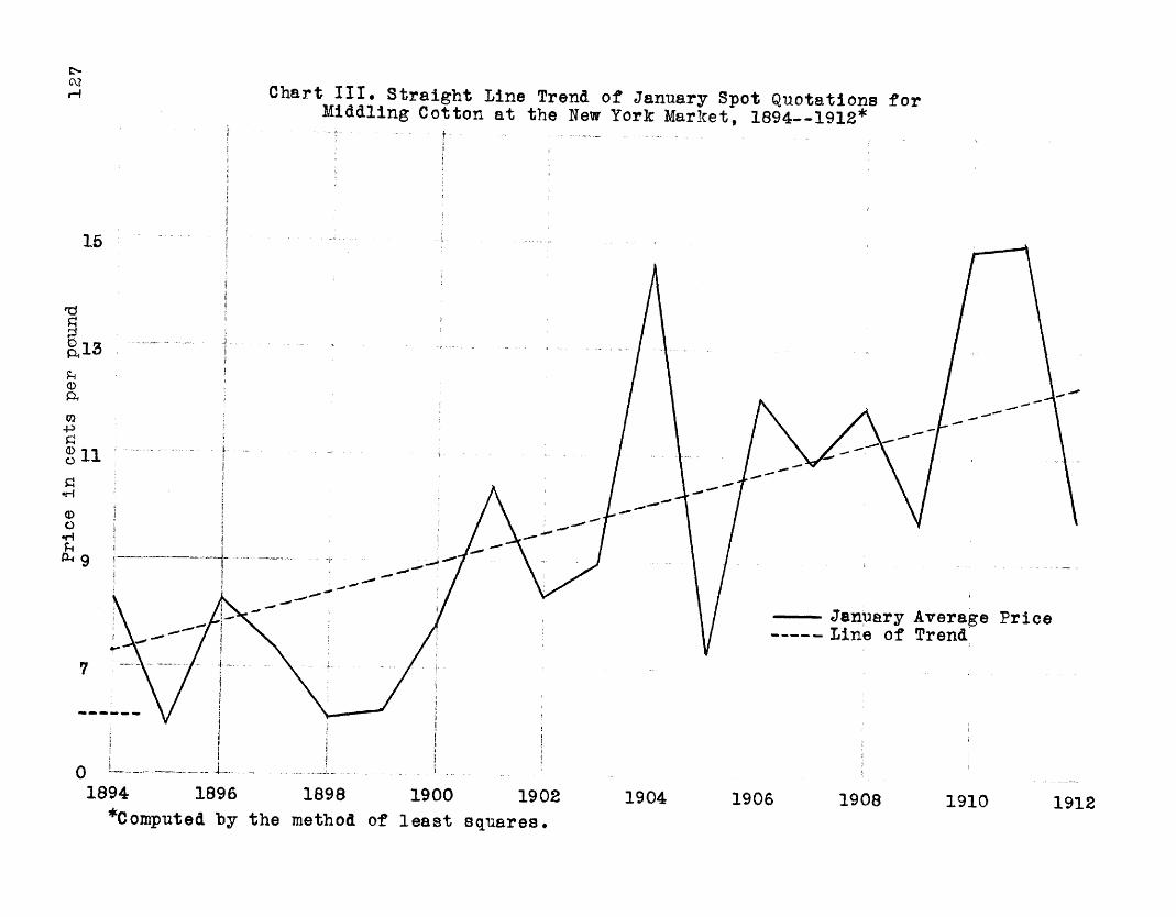
Chart III* Straight Line Trend of January Spot Quotations forMiddling Cotton at the New York Market, 1894 1912*

5

-P11

•H

♦HU^ 9

January Average Price Line of Trend

--L.1896 1898

'Computed hy the method of least squares1894 1900 1902 1904 1906 1908 1910 1912

Price

in cents

per

pound

128 Chart IV. Straight Line Trend of February Spot Quotations for

Middling Cotton at the New York Market, 1894— 1912*

i

14

— February Average Price !- Line of Trend |

1894 1896 1898 1900 1902 1904 1906 1908 1910 1912*Computed by the method of least squares.

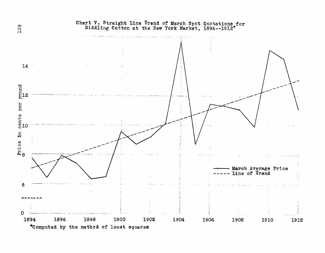
Chart V, Straight Line $rend of March Spot Quotations forMiddling Cotton at the New York Market, 1894— 1912*

14

12

10

March Average Price Line of $rend

1894 1896 1898 1900 1902 1904 1906 1908 1910 1912^Computed by the method of least squares

o Chart VI. Straight Line Trend of April Spot Quotations for3 Middling Cotton at the New York Market, 1894-19IS*

14

•H

April Average Price Line of ^rend

._J__1896 1900 1902 1904 1906 19081898 1910 19121894

^Computed by the method of least squares.

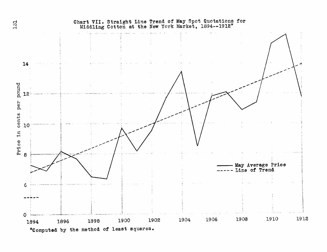
Price

in cents, per

poun

d^ Chart VII* Straight Line Trend of May Spot Quotations forh Middling Cotton at the New York Market, 1894— 1912*

14

12:

10

i—May Average Price Line of Trend

1912191019081906190419021900189818961894^Computed "by the method of least squares*

Price

in cent®

per

pound

132 Chart VIII# Straight Line Trend of June Spot Quotations for

Middling Cotton at the New York Market, 1894--1912*

14

12

June Average Price Line of Trend

1902 1906 1908 19101904 19121900189818961894^Computed hy the method of least squares.

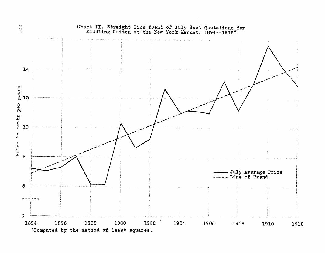
Price

in cents

per

poun

dtotoH Chart IX* Straight Line Trend of July Spot Quotations for

Middling Cotton at the New York Market, 1894— 1912*

14

12

10

July Average Price Line of Trend

1894 1896 1898 1900 1902 1904 1906 1908 1910 1912^Computed by the method of least squares*

in cents

per

pound

134 Chart X. Straight Line Trend of August Spot Quotations for

Middling Cotton at the Hew York Market, 1894— 1912*

16

14

August Average Price Line of Trend

12

♦ r i

* 10

19081904 1910 19121902 1906190018981896^Computed hy the method of least squares*

1894

Price

in cen

ts-, per

pound

3_35 Chart XI. Straight Line Trend of September Spot Quotations for

Middling Cotton at the New York Market, 1894— 1912*

14

IB

10

September Average Price Line of Trend

1900 19041896 1898 1906 19081894 1910 1912*Computed by the method of least squares.

Price

in cents

per

pound

136 Chart XII, Straight Line Trend of October Spot Quotations for

Middling Cotton at the New York Market, 1894— 1912*

14

12

101

— October Average Price Line of Trend

1900 1902 19041898 1906 19081896 19101894*Computed by the method of least squares 1912

Price

in cents' per

pound

137 Chart XIII, Straight Line Trend of November Spot Quotations for

Middling Cotton at the New York Market, 1894— 19IE*

14

IE

10

— November Average Price j- - Line of Trend i

1896 1898Computed by the method of least squares

19021894 1900 1904 1906 1908 1910 1913

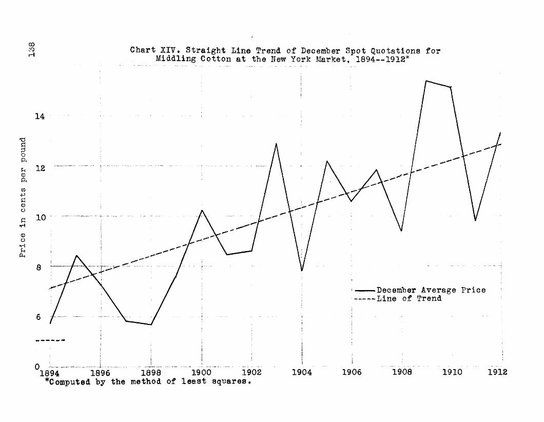
Price

in cents

per

poun

d

Chart XIV# Straight Line Trend of December Spot Quotations forMiddling Cotton at the New York Market, 1894— 1912*

14

12

10

— December Average Price — Line of Trend

19081906 1910 191219041900 190218981894Computed by the method of least squares#

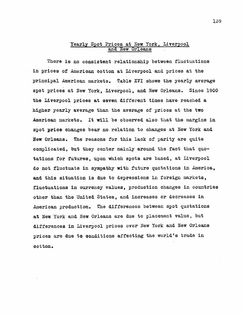
139

Yearly Spot Prices at Hew York, Liverpool an<3- ^ew Orleans

There is no consistent relationship "between fluctuations in prices of American cotton at Liverpool and prices at the principal American markets, Table XVI shows the yearly average spot prices at Hew York, Liverpool, and Hew Orleans, Since 1900 the Liverpool prices at seven different times have- reached a higher yearly average than the average of prices at the two American markets. It will be observed also that the margins in spot price changes bear no relation to changes at Hew York and Hew Orleans, The reasons for this lack of parity are quite complicated, but they center mainly around the fact that quo­tations for futures, upon which spots are based, at Liverpool do not fluctuate in sympathy with future quotations in America, and this situation is due to depressions in foreign markets, fluctuations in currency values, production changes in countries other than the United States, and increases or decreases in American production. The differences between spot quotations at Hew York and Hew Orleans are due to placement value, but differences in Liverpool prices over Hew York and Hew Orleans prices are due to conditions affecting the world’s trade in cotton.

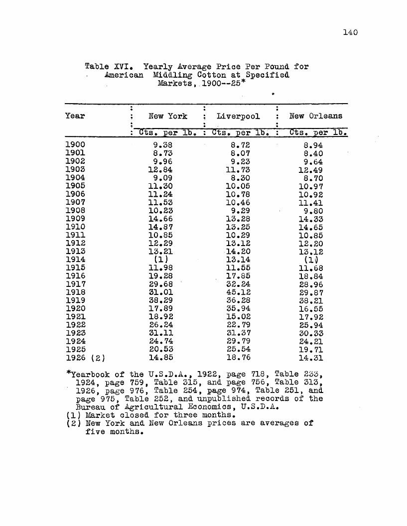
140

Table XVI* Yearly Average Price Per Pound for .American Middling Cotton at Specified

Markets,.1900— 25*

Year ; New York Liverpool ? New Orleans: Gts. per lb* Cts* per lb* : Cts. per lb.

1900 9.38 8.72 8.941901 8*73 8.07 8.401902 9.96 9.23 9.641903 12.84 11.73 12.491904 9.09 8.30 8.701905 11.30 10.05 10.971906 11.24 10.78 10.921907 11.53 10.46 11.411908 10.23 9.29 9.801909 14.66 13.28 14.331910 14.87 13.25 14.651911 10.85 10.29 10.851912 12.29 13.12 12.201913 13.21 14.20 13.121914 (1) 13.14 (101915 11.98 11.55 11.681916 19.28 17.85 18.841917 29.68 32.24 28.961918 31.01 45.12 29.871919 38.29 36.28 38.211920 17.89 35.94 16.551921 18.92 15.02 17.921922 26.24 22.79 25.941923 31.11 31.37 30.331924 24.74 29.79 24.211925 20.53 25.54 19.711926 (2) 14.85 18.76 14.31*Yearbook of the U.S.L.A., 1922, page 718, Table 233, 1924, page 759, Table 315, and page 756, Table 313, 1926, page 976, Table 254, page 974, Table 251, and page 975, Table 252, and unpublished records of the Bureau of Agricultural Economics, U.S.L.A.

Cl) Market closed for three months*(2) New York and New Orleans prices are averages of

five months*

141

Standard. Deviation of Monthly Spot " Prices ~at~ New York

The standard deviation is a measure of the extent to which items deviate from their mean* In Table XVII are shown the standard deviation of monthly spot prices of cotton at the Uew York: Market. The calculations are based on the percentage change of first differences. The magnitudes of these measures of dispersion decline from January to June, after which they increase. This indicates, to a certain extent, that there is a lower degree of causal relationship between production and price of cotton during the growing season than there is after the size of the crop is fairly accurately known. It is to be expected that deviations from the mean of prices for those months showing the greatest relationship to production will be greater than the deviations for .those months showing a less degree of relationship, particularly since changes in production are not constant from year to year.

142

fable XVII, Standard Deviation of MonthlyCotton Prices at-the Efew York

Market, 1892— 1912*

Month Standard Deviation

January 32.53February 27.90March 27.92April 25.26May 22.41June 17.47July 20.00August 22.00September 23.87October 23.71November 26.07December 32.20

*Computed from the square of the deviations from the _mean of percentage changes*

143

Coefficients of Correlation Between Production and Price of Cotton

All coefficients of correlation between production and price of cotton are calculated by the percentage change of first differ­ence method, with the exception of those in Table E, following Table XXIX* This method removes practically all the trend, which is. an important analytical procedure in formulating estimating equations* In the calculations in Table E the Pearsonian method was used, since the sole aim is to show the general tendencies of price movements in relation to production since 1920*

Table XVIII shows the coefficients of correlation between production of cotton in the United States and yearly prices at Uew York, Kew Orleans, and Liverpool for different periods of time. Tables XIX to XXV, inclusive, show the results of analysis for the period 1893-1913 at Uew York; Tables XXVI to XXVIII, inclusive, show the results for the period 1900-13 at Uew York and Uew Orleans, and Table E shows the coefficients of correlation between production in the United States, India, and Egypt and prices at Uew York for the period 1920-27*

Particular attention is called to the differences in relation­ship between production and deflated prices and production and un­deflated prices. Tables XXIII and XXIV bear out more fully the fallacies involved in attempting to remove from actual prices by deflation the changes in general price level* Cotton, itself, enters into the composite index number of the Bureau of Labor Statistics, but the changes in cotton prices from month to month

144

do not bear the same relation to monthly price index numbers asthe changes in index nuiabers bear to each other*

For each coefficient of correlation there is expressed the corresponding probable error, which means that if many similar samples were taken, half of the coefficients of correlation found would, on the average, if the differences between samples be duemerely to random selection, fall within the range r plus orminus the probable error#

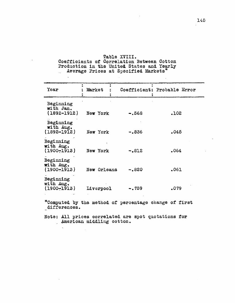
145

Table XVIII.Coefficients of Correlation Between Cotton Production in the United. States and Yearly

Average Prices at Specified Markets*

Year Market Coefficient Probable Error

Beginning with Jan. (1892-1912)Beginning with Aug. (1892-1912)Beginning with Aug. (1900t1913)Beginning with Aug. (1900-1913)Beginning with Aug. (1900-1913)

Mew York -.568

Mew York -.836

lew York -.812

Mew Orleans -.820

Liverpool -.759

.102

.045

.064

.061

.079

^Computed by the method of percentage change of first differences.

Mote: All prices correlated are spot quotations for American middling cotton.

146

Table XIX.Coefficients of.Correlation Between Cotton , Production in the United States ®nd the

Subsequent Prices of Cotton on the .. Uew York Market, 1892— 1912*

Month Coefficient of Probable ErrorCorrelation

January -.857 .041February -.889 .032March -.831 .047April -.527 .109May -.699 .078June -.627 .093July (1) -.217 .146August -.309 .139September -.537 .108October -.685 .081November -.851 .041December —. 8 71 .036

*Computed by the method of percentage change of first differences.(1) July of the current harvest year.

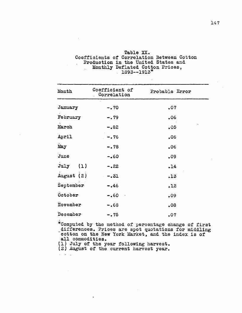
14 7

Table XX.Coefficients of Correlation Between Cotton

Production in the United States and Monthly Deflated Cotton Prices,

. 1893— 1913*

Month Coefficient of Probable Error. Correlation

January -.70 .07February -.79 .06March -.82 .05April -.76 .06May -.78 .06June i • cr> O .09July (1) -.22 .14August (2) -.31 • 13September -.46 .12October t . <7> O .09November -.68 .08December -.75 .07*Computed by the method of percentage change of first differences. Prices are spot quotations for middling cotton on the Uew York Market, and the index is of all commodities.(1) July of the year following harvest.(z) August of the current harvest year.

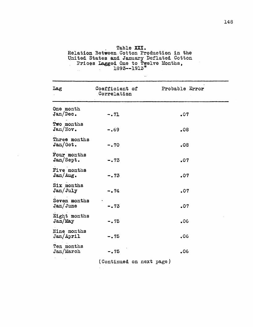
148

Table 2X1.Relation Between. Cotton Production in the United States and.January Deflated Cotton

Prioes Lagged One to Twelve Months, 1893— 1913*

Lag Coefficient of Correlation

Probable Error

One month Jan/Dec.Two months Jan/Hov.Three months Jan/Oct.Pour months Jan/Sept.Five months Jan/Aug.Six months Jan/JulySeven months Jan/JuneEight months Jan/MayUine months Jan/AprilTen months Jan/March

-.71

-.69

-.70

-.73

-.73

-.74

-.73

-.75

-.75

.07

.08

.08

.07

.07

.07

.07

.06

.06

-.75 .06(Continued on next page)

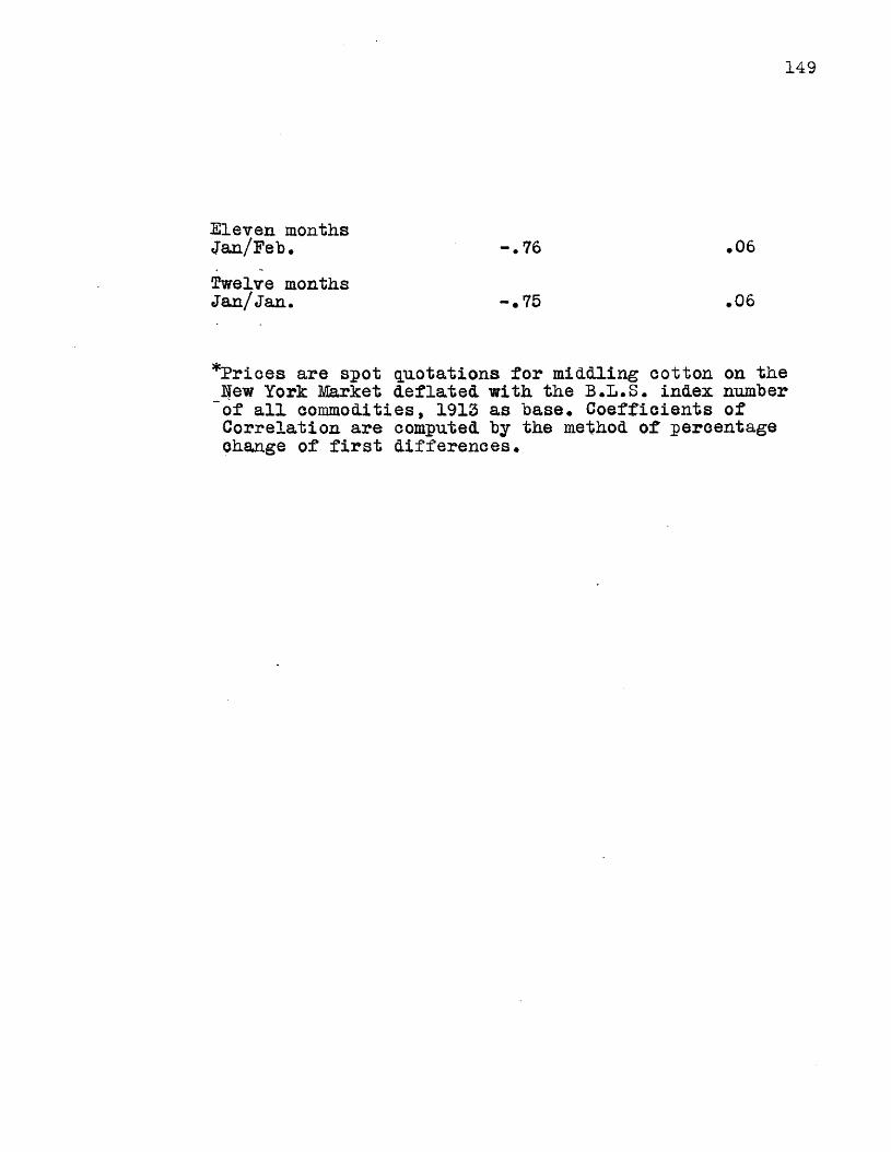
149

EleYen monthsJan/Feb. -.76 .06(Twelve monthsJan/Jan. -.75 .06

*Prices are spot quotations for middling ootton on the _New York Market deflated with the B.L.S. index number "of all commodities, 1913 as base. Coefficients of Correlation are computed by the method of percentage Change of first differences.

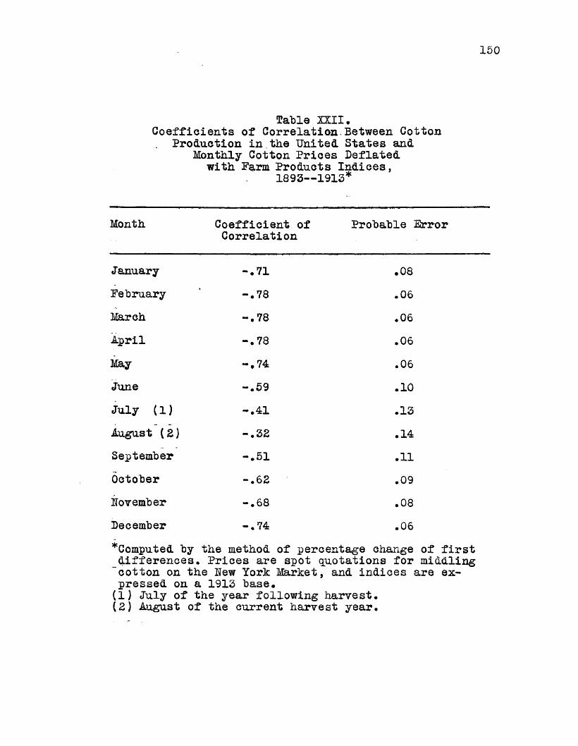
150

Table XXII.Coefficients of Correlation.Between Cotton

Production in the United States and Monthly Cotton Prices Deflated

with Farm Products Indices, 1893— 1913*

Month Coefficient of Probable ErrorCorrelation

January -•71 .08February -•78 .06March -.78 .06April -.78 .06May -.74 .06June -.59 .10July (1) —. 41 .13August (2) -.32 .14September -.51 .11October -.62 .09November -.68 .08December -.74 .06^Computed by the method of percentage change of first differences* Prices are spot quotations for middling cotton on the Uew York Market, and indices are ex­pressed on a 1913 base*(1) July of the year following harvest.(2) -August of the current harvest year*

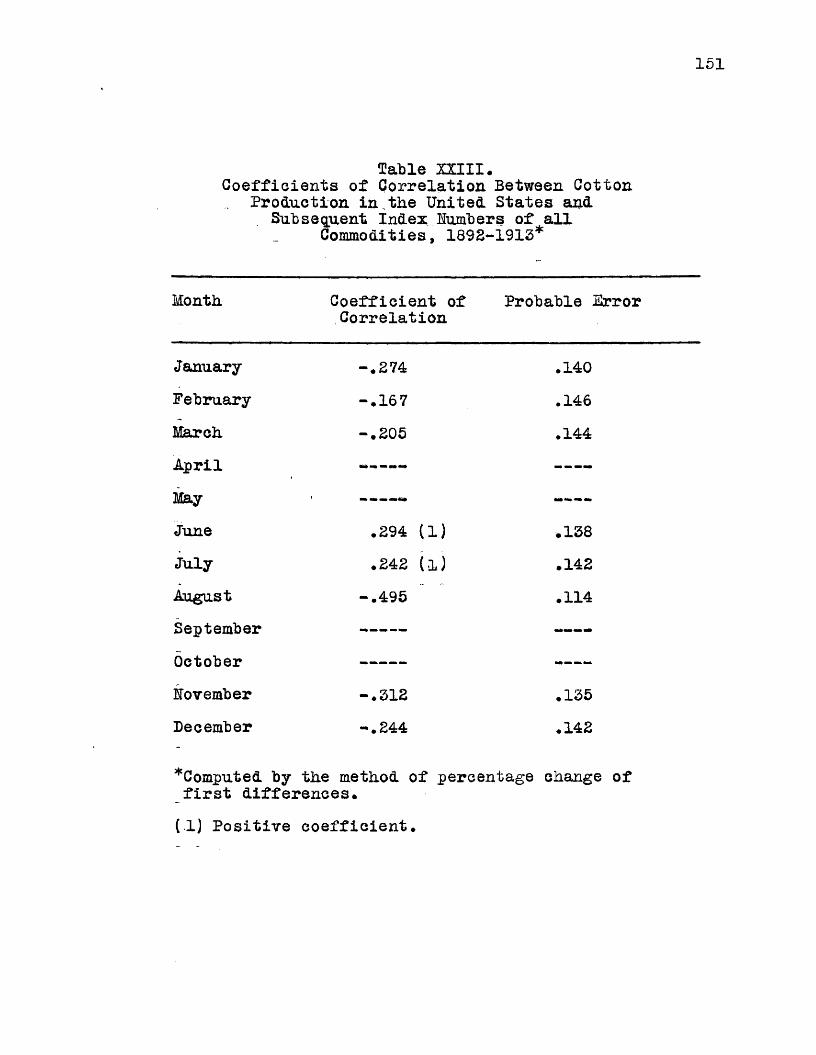
151

Table XXIII*Coefficients of Correlation Between Cotton

Production in,the United States and Subsequent Index Numbers of sill

Commodities, 1892-1913*

Month Coefficient of Probable ErrorCorrelation

January -.274 .140February -.167 .146March -.205 .144April ----

May ----

June .294 (1) .138July .242 (oJ .142August -.495 .114September ----

October ----

November -.312 .135December -.244 .142

*Computed by the method of percentage change of first differences.(1) Positive coefficient.

152

Table XXIV.Coefficients of Correlation Between Yearly

Index numbers of all Commodities and . the Subsequent Prices of Cotton,

1893— 1913*

Month Coefficient of Probable ErrorCorrelation

January .551 .107February .567 .105March .360 .134April .363 .134May .305 .136June .482 .119July ---- ----

August ---- ----

September ---- ----

October -.361 (1) .134November ---- — -December -.301 (1) .140^Computed by the method of percentage change of first differences. Prices are spot quotations for middling cotton on the Sew York Market#(1) negative coefficient.

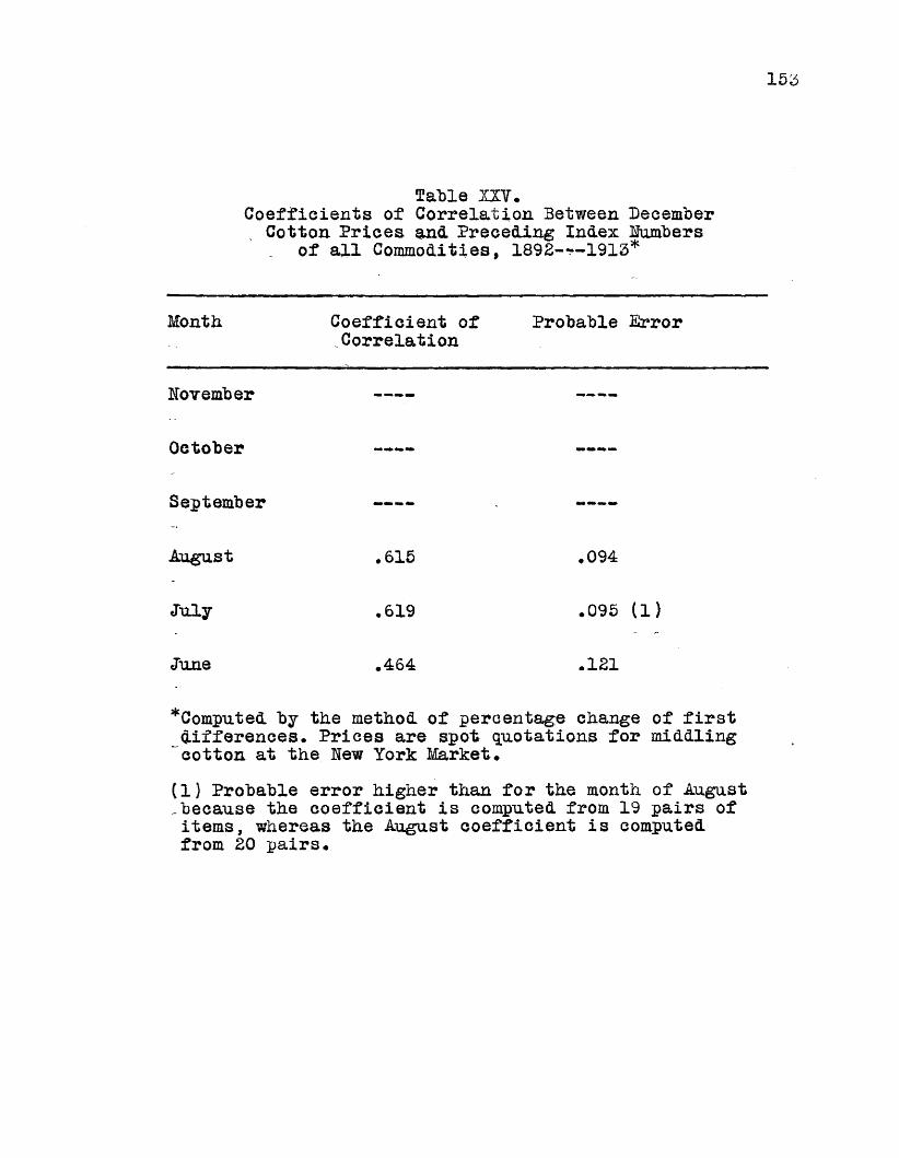
153

Table XXV.Coefficients of Correlation Between December

Cotton Prices and Preceding Index Numbers of all Commodities, 1892-^-1913*

Month Coefficient of Probable ErrorCorrelation

November

Oetober

September

August *615 *094

July .619 .095 (1)

June *464 .121

^Computed by the method of percentage change of first differences. Prices are spot quotations for middling cotton at the New York Market.(1) Probable error higher than for the month of August .because the coefficient is computed from 19 pairs of items, whereas the August coefficient is computed from 20 pairs.

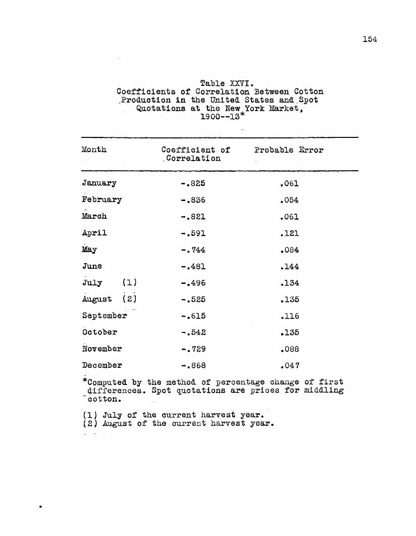
154

T a b l e 2X71.Coefficients of Correlation Between Cotton production in the United States and.Spot

Quotations at the New York Market, 1900— 13*

Month Coefficient of Probable Error.Correlation

January -.825 .061February -.836 .054Miareh -.821 .061April -.591 .121May -.744 .084June -.481 .144July (1) -.496 .134August (2) -.525 .135September -.615 .116October -.542 .135November -.729 .088December -.868 .047^Computed by the method of percentage change of first differences* Spot quotations are prices for middling “cotton.(1) July of the current harvest year.[Z) August of the current harvest year.

155

Table XXVII.Coefficients of Correlation Between Cotton

Production iti the United. States and Prices at the Dew Orleans Market,

1900— 13*

Month Coefficient of Probable Error.Correlation

January -.392 .069February -.826 .060March -.818 .062April -.799 .067May -.554 .128June -.461 .135July (1) -.398 .162August (2) -.554 .128September -.545 .131October -.567 .127November -.733 .086December -.837 .056*Computed by the method of percentage change of first differences. Prices are spot quotations for middling cotton.(1) July of the current harvest year.(2j August of the current harvest year.

156

Table XEVTII.Coefficients of.Correlation Between Cotton

Production in the United States and Deflated Cotton Prices at the Uew

York Market, 1900— 13*

Month Coefficient of Probable ErrorCorrelation

January -.768 .077February -.815 .062March -.807 .065April -.809 .065May -.779 .073June -•60S .112July (1) -.375 .161August (£) -.557 .128September -.743 .084October -.503 .135November -.773 .073December -.902 .036*Computed by the method of percentage change of first differences* Prices deflated with B.L.S. index number, 1890-99 base*(1) July of the current harvest year.(2j August of the current harvest year.

157

Table XXIX.Coefficients of.Correlation Between Monthly Prices of Cottpn at lew York and Total

Cotton Production of the United States, India, and Egypt,

1900— 13*

Month Coefficient of Probable ErrorCorrelation

January -.840 .055February -.825 .061March -.813 .064April -.591 .121May -.715 .091June -.357 .163July (1) -.597 .125August -.601 .119September -.663 .105October -.458 .148lovember -.674 .102December -.876 .044^Computed by the method of percentage change of first differences. Prices are spot quotations for middling cotton.{1} July of the current harvest year.

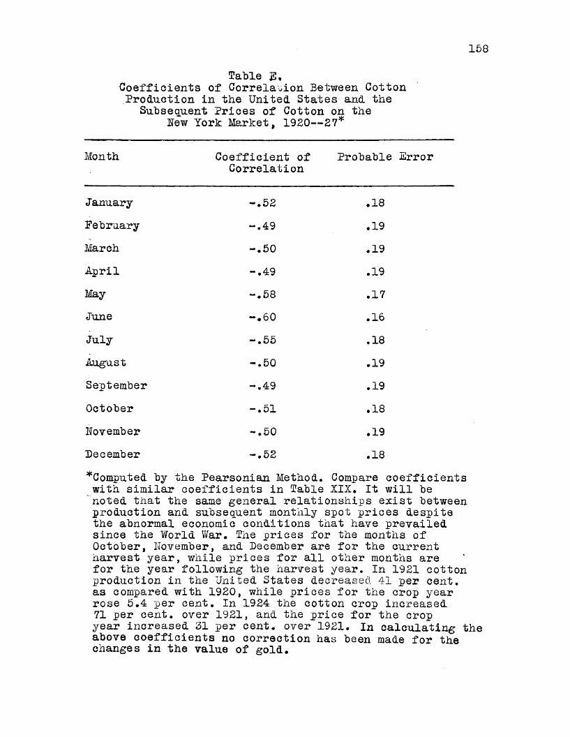
158

Table E,Coefficients of Correlation Between Cotton Production in the United States and the

Subsequent Prices of Cotton on the New York Market, 1920— £7*

Month Coefficient of Probable ErrorCorrelation

January -.52 .18February -.49 .19March 0UO.1 .19April -.49 .19May -.58 .17June -.60 • 16July -.55 .18August -.50 .19September -.49 .19October -.51 .18November oLQ.t .19December -.52 .18^Computed by the Pearsonian Method. Compare coefficients with similar coefficients in Table XIX. It will be noted that the same general relationships exist between production and subsequent monthly spot prices despite the abnormal economic conditions that have prevailed since the World War. The prices for the months of October, November, and December are for the current harvest year, while prices for all other months are for the year following the harvest year. In 1921 cotton production in the United States decreased 41 per cent, as compared with 1920, while prices for the crop year rose 5.4 per cent. In 1924 the cotton crop increased 71 per cent, over 1921, and the price for the crop year increased 31 per cent, over 1921. In calculating the above coefficients no correction has been made for the changes in the value of gold.

159

Predictive Formulas

The predictive formulas in Table XXX are developed from the equation y a Ay minus bAx plus bx, in which, y is the per­centage change in price, Ay the average of percentage change in price, x the percentage change in production, Ax the average of percentage ©hange in production, and b the coefficient of regression of y on x, calculated by dividing the standard deviation of the y series by the standard deviation of the x series and then multiplying by the coefficient of correlation between x and y*The constant, Ay minus bix, is determined by subtracting from the average of the y series the product of the coefficient of regression and the average of the x series. With the constant value deter­mined, the estimate for any one month is made by adding to the constant the product of the coefficient of regression and the percentage change in x. The regression coefficient has a minus value because, normally, the y series moves in opposite direction from the x series®

Attention is called to the fact that for months in which the prices show the highest degree of relationship to current production the constant values are greatest*

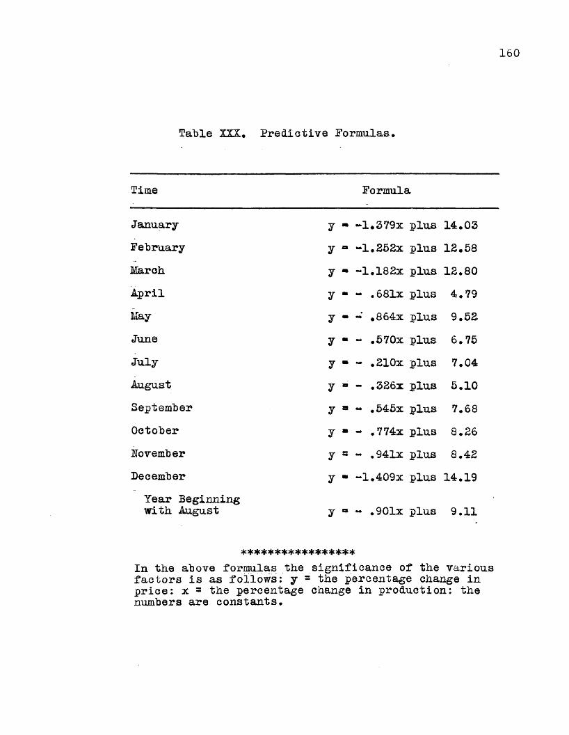
160

Table XXX* Predictive Formulas.

Time Formula

January 7 m -1.379x plus 14.03February 7 a -1.252x plus 12.58March 7 m -1.182x plus 12.80April 7 m - .681x plus 4.79May 7 m - .864x plus 9.52June 7 - - .570x plus 6.75July 7 a - .210x plus 7.04August 7 a - .326x plus 5.10September 7 a - .545x plus 7.68October 7 a - .774x plus 8.26November 7 a - .941x plus 8.42December 7 - -1.409x plus 14.19Year Beginning with August 7 a ** .901x plus 9.11

In the above formulas the significance of the various factors is as follows: y = the percentage change in price: x = the percentage change in production: the numbers are constants.

161

Price Change Estimates

Tables XXXI to XLIII, inclusive, show the actual percentage changes in yearly and monthly spot prices of cotton and the changes as estimated by means of the dynamic laws of demand for cotton expressed in the predictive formulas in Table XXX. It will be seen that there is a tendency for the more nearly accurate estimates to be associated with the high constant values in the predictive formulas, which, themselves, tend to be associated with high minus values of regression. It is to be observed in this connection that the approach to accuracy tends to vary directly with the magnitude of the regression coefficient.

Table XLI7 shows the average differences between actual and estimated changes in Uew York spot prices. In no case, it will be observed, is the error as' great as 1 per cent., taking the period as a whole. The highest average per cent, of erroroccurs in July, the month for which prices and production show

{LIthe lowest degree of negative relationship^. It necessarily follows that the lower degree of approach to accuracy in any estimate will be associated with a low degree of causal relation­ship between dependent and independent variables.

^See Table XIX for coefficients of correlation from which regression coefficients were calculated.

162

fable XXXI,The Actual Percentage Changes in Yearly AveragePrices of Cotton and. the Changes as Predicted.*

Year ActualPercentage

ChangePredicted

PercentageChange

1892-931893-94 - 8.17 — 2.081894-95 -17.55 -14.691895-96 25.66 31.001896-97 - 4.48 - 8.101897-98 -16.55 -15.861898-99 -12.50 6.711899-00 49.28 23.081900-01 12.08 1*621901-02 - 6.62 15.601902-03 12.91 1.431903-04 30.06 15.791904-05 -29.57 -23.701905-06 25.19 28.311906-07 - 1.14 -13.871907-08 4.28 23.801908-09 -12.41 - 8.201909-10 43.40 31.101910-11 1.43 - 5.291911-12 -27.28 -22.821912-13 13.58 20.55hew York spot quotations for Middling cotton.

)Jc sf: J)t Jjc ^ sf: sfc jJc sjc sfcsfc

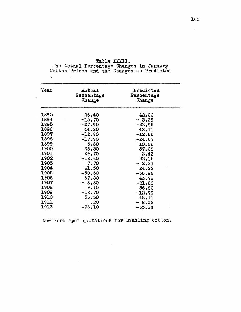
Table XXXII,The Actual Percentage Changes in January

Cotton Prices and the Changes as Predicted

Year ActualPercentage

ChangePredicted

PercentageChange

1893 26,40 42.001894 -15.70 - 3.291895 -27.90 -22.851896 44.80 48.111897 -12.80 -12.651898 -17.90 -24.671899 3.50 10.261900 28.30 37.081901 29.70 2.431902 —18*60 22.151903 7.70 - 2.311904 61.30 24.221905 -50.30 -36.821906 67.50 43.791907 - 8.80 -21.591908 9.10 36.801909 -18.70 -12.791910 53.30 48.111911 .20 - 8.321912 -36.10 -35.14

JJew York spot quotations for Middling cotton

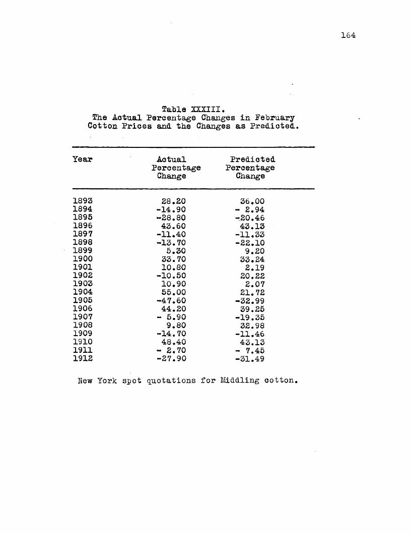
Table i n III*The Actual Percentage Changes in FebruaryCotton Prices and. the Changes as Predicted..

Year ActualPercentageChange

Predicted.Percentage

Change

1893 28.20 36.001894 -14.90 - 2.941895 “28.80 r20.461896 43.60 43.131897 -11.40 -11.331898 -13.70 -22.101899 5.30 9.201900 33.70 33.241901 10.80 2.191902 -10.50 20.221903 10.90 2.071904 55.00 21.721905 -47.60 -32.991906 44.20 39.251907 - 5.90 -19.351908 9.80 32.981909 -14.70 -11.461910 48.40 43.131911 - 2.70 - 7.451912 -27.90 -31.49

New York spot quotations for Middling cotton

Cable XXXIV*die Actual Percentage Changes in March.

Cotton Prices and the Changes as Predicted

Year ActualPercentage

ChangePredicted

PercentageChange

1893 31.70 36.801894 -14.90 - 1.851895 -18.10 -18.401896 24.80 41.641897 - 6.30 - 9.771898 -14.90 -19.941899 3.70 9.611900 52.10 32.301901 -11.80 2.991902 5.40 20.011903 9.30 “ 1.031904 60.40 21.431905 -48.11 -30.221906 40.90 37.981907 - 1.30 -17.341908 - 1.50 32.061909 -11.40 - 9.891910 53.50 41.641911 - 3.30 - 6.111912 -26.10 -28.80Uew York spot quotations for Middling cotton.

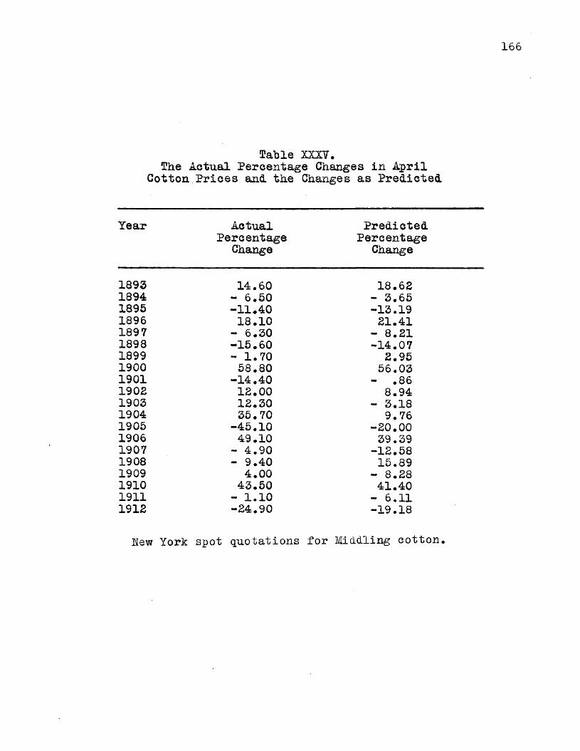
166

Table XXXV.The Actual Percentage Changes in April

Cotton Prices and. the Changes as Predicted.

Year ActualPercentage

ChangePredicted.

PercentageChange

1893 14.60 18.621894 - 6.50 - 3.651895 -11*40 -13.191896 18.10 21.411897 - 6.30 - 8.211898 -15.60 -14.071899 - 1.70 2.951900 58.80 56.031901 -14.40 - .861902 12.00 8.941903 12.30 - 3.181904 35.70 9.761905 -45.10 -20.001906 49.10 39.391907 - 4.90 -12.581908 - 9.40 15.891909 4.00 - 8.281910 43.50 41.401911 - 1.10 - 6.111912 -24.90 00 i—

I .rH1

Hew York spot quotations for Middling cotton.

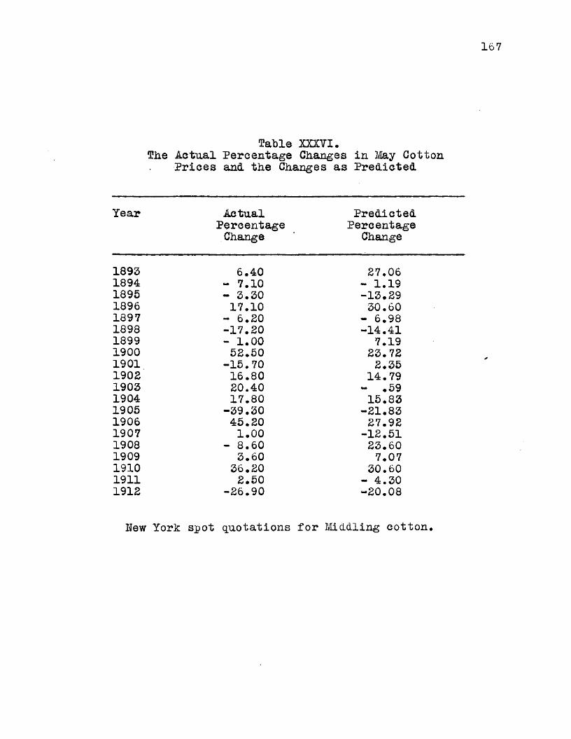
Table XXXVI.The Actual Percentage Changes in May Cotton

Prices and the Changes as Predicted

Year ActualPercentageChange

PredictedPercentage

Change

1895 6.40 27.061894 - 7.10 - 1.191895 - 3.30 -13.291896 17.10 30.601897 - 6.20 - 6.981898 -17.20 -14.411899 - 1.00 7.191900 52.50 23.721901 -15.70 2.351902 16.80 14.791903 20.40 - .591904 17.80 15.831905 -39.30 -21.831906 45.20 27.921907 1.00 -12.511908 - 8.60 23.601909 3.60 7.071910 36.20 30.601911 2.50 - 4.301912 -26.90 -20.08

Hew York spot quotations for Middling cotton.

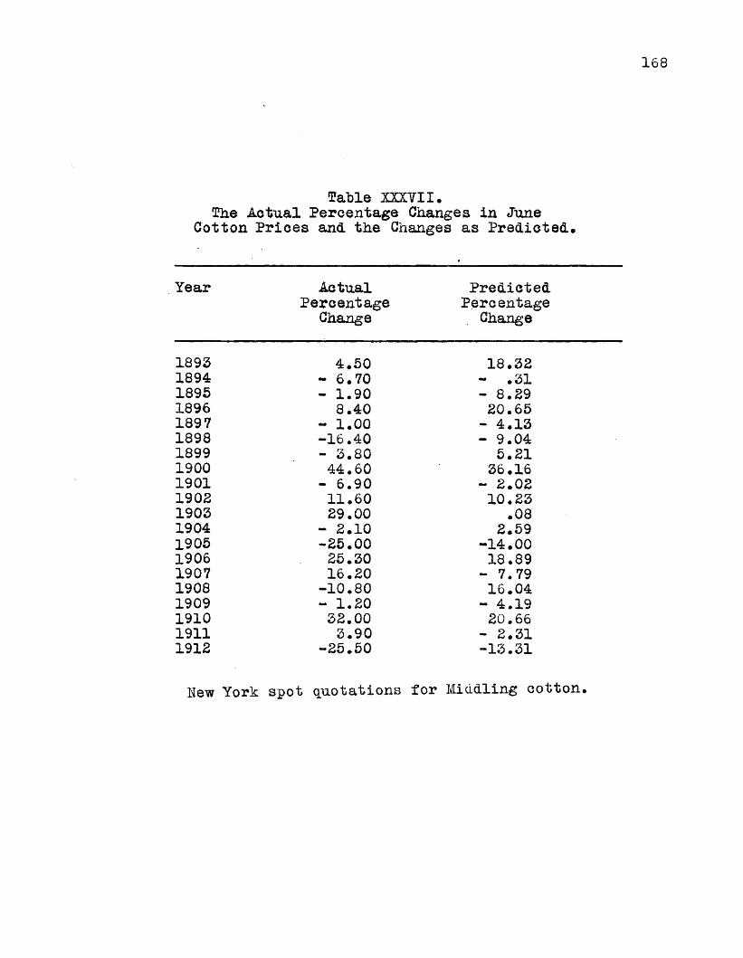
168

Eatle xmrn.The Actual Percentage Changes in June

Cotton Prices and. the Changes as Predicted.,

Year ActualPercentage

ChangePredicted

Perc entage Change

1893 4.50 18.321894 - 6.70 - .311895 - 1.90 - 8.291896 8.40 20.651897 - 1.00 - 4.131898 -16.40 - 9.041899 - 3.80 5.211900 44.60 36.161901 - 6.90 - 2.021902 11.60 10.231903 29.00 .081904 - 2.10 2.591905 -25.00 -14.001906 25.30 18.891907 16.20 - 7.791908 -10.80 16.041909 - 1.20 - 4.191910 32.00 20.661911 3.90 - 2.311912 -25.50 -13.31

New York spot quotations for Middling cotton.

T qJqI q XXXVIII.9?he Actual Percentage Changes in July

Cotton.Prices and the Changes as Predicted.

Year ActualPercentageChange

PredictedPercentage

Change

1893 9.80 11.301894 -11.40 4.431895 - .90 1.501896 2.70 12.161897 9.80 3.03 ,1898 - 9.90 1.221899 - .10 6.571900 64.30 10.511901 -14.10 5.341902 8.10 8.321903 36.10 4.581904 -13.60 8.571905 .80 .601906 - .80 11.511907 19.70 1.681908 -15.60 10.461909 16.20 3.061910 23.20 12.161911 -11.10 3.681912 - 9.40 - .35

New York spot quotations for Middling cotton.

170

Table XXXIX.The ActuaX Percentage Changes in AugustCotton Prices and the Changes as Predicted

Year ActualPercentage

ChangesPredicted

PercentageChange

1893 5.20 - .061894 - 8.70 - 3.511895 9.20 13.051896 5.60 11.331897 0.00 - 3.931898 -26.20 4.221899 5.60 10.481900 57.30 2.391901 -15.90 7.091902 8.70 1.291903 42.30 7.481904 -14.60 - 6.771905 .30 12.041906 - 5.70 - 3.211907 .80 10.411908 -23.20 - 1.161909 24.50 13.051910 27.30 - .111911 -24.10 - 6.381912 - 2.80 9.24

Hew York spot quotations for Middling cotton.

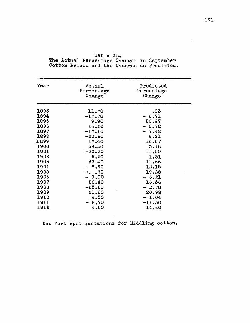
Table XL*The Actual Percentage Changes in September Cotton Prices and the Changes as Predicted.

Year ActualPercentage

ChangePredicted

PercentageChange

1893 11.70 .931894 -17.70 - 6.711895 9.90 20.971896 15.20 - 2.721897 -17.10 - 7.421898 -20.60 6.211899 17.40 16.671900 59.50 3.161901 -20.30 11.001908 6.50 1.311903 32.40 11.661904 - 7.70 -12.151905 .70 19.281906 - 9.90 - 6.211907 28.40 16.561908 -25.20 - 2.781909 41.60 20.981910 4.50 - 1.041911 -18.70 -11.501912 4.60 14.60

Hew York spot quotations for Middling cotton

172

Table XII.The Actual Percentage Changes In OctoberCotton Prices and the Changes as Predicted.

Year ActualPercentage

ChangePredicted

PercentageChange

1893 2.90 - 1.341894 -27.40 -12.171895 49.00 27.151896 -11.10 - 6.251897 -20.80 -13.181898 -14.30 6.171899 34.80 21*031900 25.80 1.841901 -15.10 12.981902 4.50 - .791903 10.20 13.911904 6.80 -19.911905 13.00 25.741906 6.90 -11.741907 .40 20.871908 -11.80 - 6.601909 51.40 27.151910 4.30 - 4.121911 -32.80 -18.981912 15.00 18.09

Hew York spot quotations for Middling cotton.

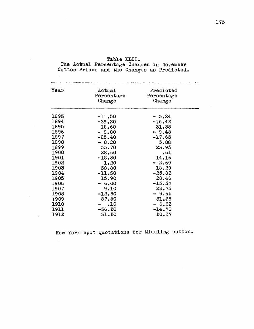
Table XLII.The Actual Percentage Changes in November Cotton Prices and the Changes as Predicted#

Year ActualPercentageChange

PredictedPercentage

Change

1893 -11.50 — 3.241894 -29.20 -16.421895 15.60 31.381896 - 8.80 — 9.451897 -25.40 -17.651898 - 8.20 5.881899 33.70 23.951900 28.60 • 611901 -18.80 14.161902 1.20 - 2.691903 38.80 15.291904 -11.30 -25.831905 15.90 28 *461906 - 6.00 -15.571907 9.10 23.751908 -12.80 - 9.651909 57.50 31.381910 - .10 - 6.631911 -36.20 -14.701912 31.20 20.37

Hew York spot quotations for Middling cotton#

174

Table XLIII.The Actual Percentage Changes in DecemberCotton Prices ancL the Changes as Predicted.

Year Actual PredictedPercentage Percentage

Change Change

1893 -19.00 - 3.281894 -27.60 -13.01IL895 46.20 48.571.896 -13.75 -12.721897 -18.15 -24.841898 - 3.39 10.391.899 34.40 37.441900 33.00 2.502.901 -16.90 22.781902 1.77 - 2.301903 50.93 24.481904 -40.82 -37.101905 58.00 44.191906 -12.35 -21.741907 12.30 37.161908 -22.78 -12.861909 65.60 48.561910 - 1.53 - 8.351911 -37.20 -35.411912 37.80 32.79

Hew York spot quotations for Middling cotton*

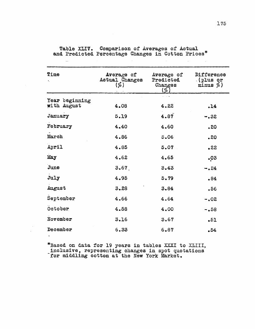
175

Table XLIV. Comparison of Averages of Actualand Predicted Percentage Changes in Cotton Prices*

Time Average of Average of DifferenceActual Changes Predicted -(plus or ($)__________ Changes_______minus jo)

Year beginning with August 4.08 4.22 ♦14January 5.19 4.87' -.32February 4.40 4.60 .20March 4.86 5.06 .20April 4.85 5.07 ♦ 22May 4.62 4.65 .03•June 3.67. 3.43 -.24July 4.95 5.79 . 00

August 3.28 3.84 .56September 4.66 4.64 i . o toOctober 4.58 4.00 -.58November 3.16 3.67 • 51December 6.33 6.87 .54

*Based on data for 19 years in tables XXXI to XLIII, inclusive, representing changes in spot quotations for middling cotton at the Etew York Market*

176

Graphic Presentation of Actual and EstimatedChanges in Price

Charts XV to XXVII, inclusive, present more clearly the conception of estimates of price changes as influenced "by size of crop. The actual percentage changes and the changes as estimated are plotted together, and the reader can readily see the degree of approach to accuracy. These changes are plotted in terms of percentages, since the coefficients of correlation were calculated by the percentage change of first difference method. They are, for that reason, the quantities in which we are most interested.

These charts show graphically the data presented in Tables XXXI to XLIII, inclusive. Here, again, will be observed the fact that the greatest degree of approach to accuracy of estimate is attained after the size of the crop is known. From planting time until the probable size of the subsequent crop is known there is less tendency for high or low prices to be associated with preceding low or high production. This is simply an example of the concept involved in the economic laws of supply, potential supply, and demand, and it illustrates the principle that for short periods of time prices are determined by factors other than elements of cost*

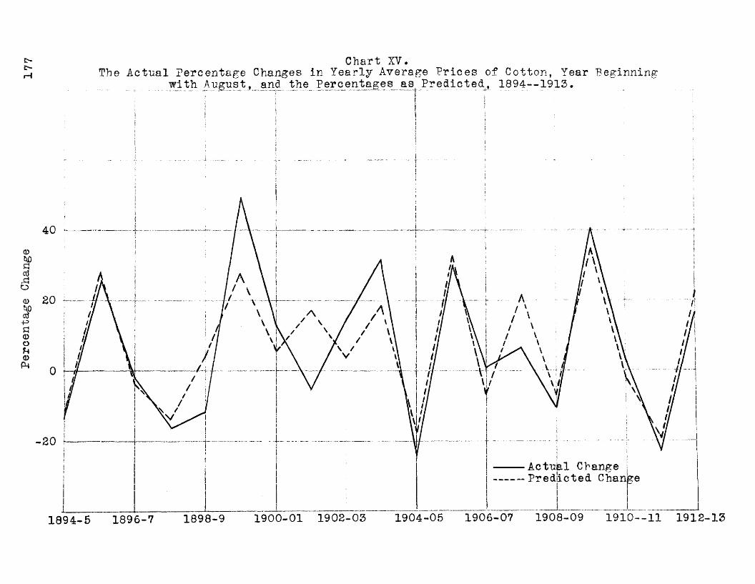
Percentage

Change

177 Chart XV.

The Actual Percentage Changes in Yearly Average Prices of Cotton, Year Beginningwith August, and the Percentages as Predicted, 1894— 1915

40

20

-20Ac tula 1 Change j Predicted Chanp

1908-09 1910--11 1912-151904-05 1906-071900-01 1902-051898-91894-5 1896-7

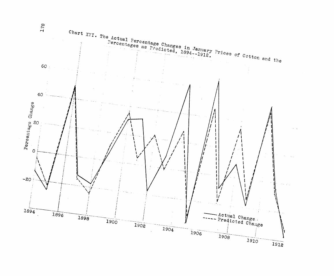
CD£NH

I j -' ■- LZOn ana the60

Percentage

Change

Chart XVII. The Actual Percentage Changes in February Prices of Cotton and theh Percentages as Predicted, 1894--1912.

1 " F

6

30

15

-15

Actual Change; Predicted Change

19061902 1904 1908 19101900 1912' 189818961894

Percentage

Change

0 Chart XVIII# -he Actual Percentage Changes in March Prices of Cotton and the3 Percentages as Predicted, 1894--1912r H

60

40

20

-20— Actjual Changej— Prejdicted Chajng

4019041902 190819061900 19101898 191218961894

Percentage

Change

]_q]_ Chart XIX. The Actual Percentage Changes in April Prices of Cotton and the

Percentages as Predicted, 1894— 1912.

60

40

20

Actual Chanfee Predicted Change-40

1908 1910 19121906190419021900189818961894

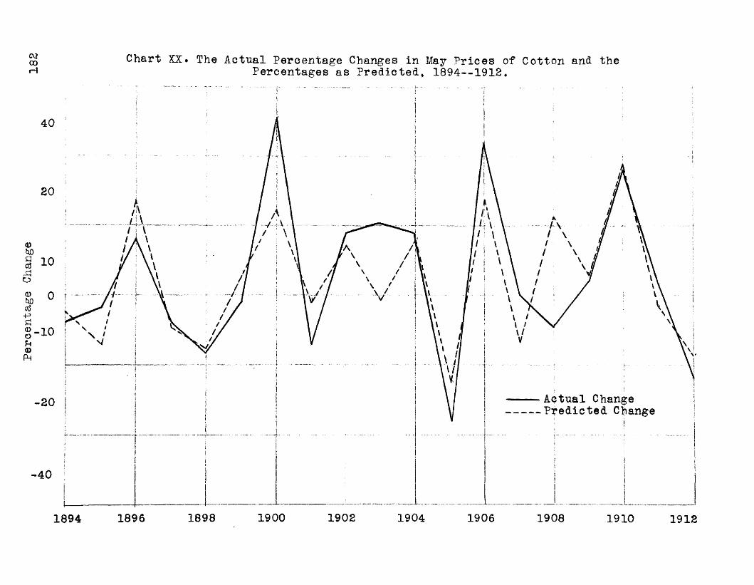
Percentage

Change

Chart XX. The Actual Percentage Changes in May Prices of Cotton and thePercentages as Predicted, 1894— 1912.

40

20

/ h /\

10

\ /0

Actual Change Predicted Change20

40

1900 19041898 1902 1908190618961894 1910 1912

Percentage

Change

Chart XXI. The Actual Percentage Changes in June Prices of Cotton and thePercentages as Predicted, 1894--1912.

rH

40

20

10v

0 t

— Aotual Change -- Predicted Change20

1908 1910 19121906190419021900189818961894

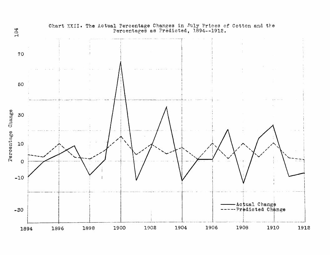
Percentage

Change

Chart XXII# The Actual Percentage Changes in July Prices of Cotton and the §5 Percentages as Predicted, 1894--1912.i— i

70

50

30

10

10

Acjtual Change Predicted Change30

1908 19101902 1904 19061900 1912189818961894

Percentage

Change

lQh Chart XXIII. The Actual Percentage Changes in August Prices of Cotton and the

Percentages as Predicted, 1894--1912.

70

Actual Change Predicted Change50

50

10

0

10

30

19061904 19101902 19081900 1912189818961894

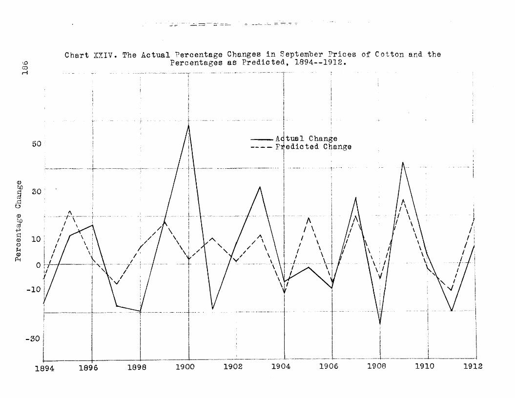
Percentage

Change

Chart XXIV. The Actual Percentage Changes in September Prices of Cotton and thePercentages as Predicted, 1Q94--1912.

Actual Change Predicted Change50

so:

10

so

19081906 1910 1912190419021900189818961894

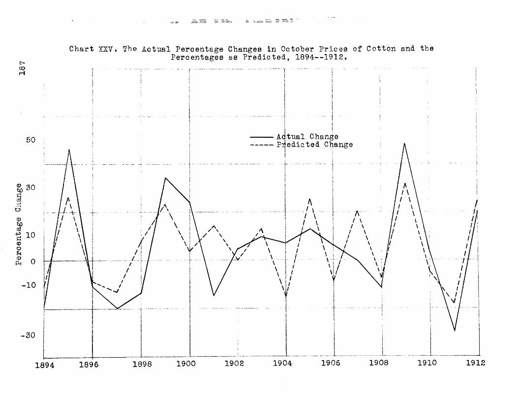
Percentage

Change

o00rH

Chart XXV. The Actual Percentage Changes in October Prices of Cotton and thePercentages as Predicted, 1894--1912.

— Acitual Change— Predicted Change50

30

10

0

10

30

1908 19101906 1912190419021900189818961894

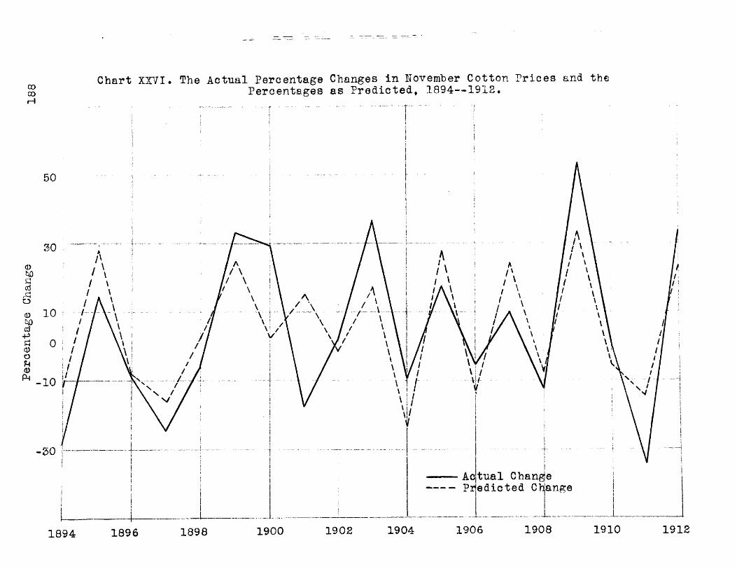
Chart XXVI. The Actual Percentage Changes in November Cotton Prices and thePercentages as Predicted* 1894— 1912,rH

50

50a>CJaJo0) 10UQ c s i -Ps 0<DOU<D* -10

V

jtual Change Jedicted Change

AcjPr|-

1908 1910 19121906190419021900189818961894

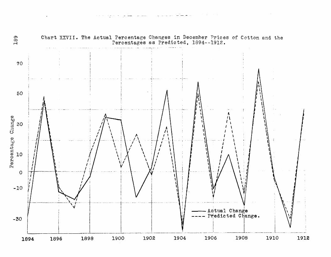
Percentage

Change

g Chart XXVII. The Actual Percentage Changes in December Prices of Cotton and theh Percentages as Predicted, 1894--1912.

70

50

30

10

10

AQtual Change Predicted Change-30

1910190819061904 191219021900189818961894

190

Standard Errors of Estimate of Priee Changes

The standard errors of estimate in Table XLV are expressionsof the degree of accuracy of price change estimates as made by the predictive formulas in Table XXX* These measures have sig­nificance in that when a distance equal to the standard error islaid off on each side of the mean in a normal or only slightlyskewed distribution about two-thirds of the estimates will be included*

The standard error is calculated by extracting the square root of the mean-square-deviations of estimated changes from actual changes. It is significant to note that the magnitudes of the standard errors of estimate in Table XLV are less than the standard deviations of actual changes in Table XVII f meaning that the estimated percentage changes deviate less from the actual changes than the actual changes deviate from their res­pective means. The reader will observe further that the differ­ence between standard error and standard deviation diminishes from time of planting of the cotton crop to the time that the probable size of the current crop is indicated or known. This implies that there is likely to be less degree of accuracy in price predictions for the latter months of the harvest year, since potential current production, even as soon as the acreage planted is known to the cotton trade, exerts an influence upon price.

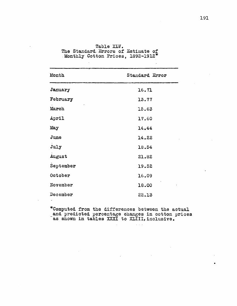
191

Table XIV.The Standard.- Errors of Estimate of Monthly Cotton Prices, 1892-1912*

Month Standard. Error

January 16.71February 13.77March 15.63April 17.60May 14.44June 14.22July 18.54August 21.82September 19.52October 16.09November 18.00December 22.13

*Computed from the differences between the actual and predicted percentage changes in cotton prices as shown in tables XXXI to XLIII, inclusive.

192

Factors Related to Cotton Prices

Cotton prices, being a component part of the compositeindex of general price level, are generally directly relatedto prices of other commodities. In the case of certain pricesthis direct relationship is particularly marked, especiallywith such commodities as are used for the same purposes as cotton,and those that reflect general business conditions as a whole*

Table XLYI shows the coefficients of correlation betweenmonthly wool prices and the subsequent monthly prices of cotton.These expressions of relationship show that five to seven monthsafter a rise or fall in the price of wool a corresponding riseor fall may be anticipated in the price of cotton* The same

%

general degree of relationship prevails between silk prices and subsequent prices of cotton, the latter being lagged five to seven months. The reader, however, will not construe these associ­ated relationships to mean there is an equal degree of causal relationship between the factors. The extent, if any, to which wool and silk are substituted for cotton involves the concept of consumer preference and effective demand, as well as the tendency toward increased consumption of rayon. As a matter of fact, theper capita consumption of all these materials cotton— wool--silk— rayon--has tended to increase, and it would require avery detailed and comprehensive analysis of market conditions to determine the extent to which the demand for one is reflected in the price of another.

193

Table XLYII shows the coefficients of correlation between industrial stocks and the prices of cotton thirteen months later. These are expressions of relationship between one type of general business conditions and cotton prices, showing that a change in prices of industrial stocks is not evidenced to any great extent in cotton prices until about a year later. This is graphically shown in Chart 2XVIII#

Other measures of general business conditions are reflected in bank clearings and pig iron production* Cotton prices tend to move simultaneously with the former, and with a lag of about seven months with the latter. Table XLVIII shows the coefficients of correlation between monthly pig iron production in the United States and monthly cotton prices* It will be observed that on an average the latter are associated with the former to approxi­mately the same degree as with the prices of industrial stocks.

194

Table XLVIRelation Between Monthly Wool Prices and the Subsequent Monthly Prices of Cotton, 1900-13*

Coefficient of Correlation Humber of Month Between Wool Prices and the Months lag____________ Subsequent Prices of Cotton______________January • 55 7February • 64 6March .72 5April .55 6May • 70 7June • 73 6July .66 4August .63 3September .70 2October • 67 1Hovember .48 0December .41 8^Coefficients have been computed by the method of per­centage change of first differences, and they are based on wool prices at the Boston Market as published in the 1924 U.S.D.A, Yearbook, page 958, Table 569, and deflated spot quotations for middling cotton at Hew York, In this analysis the coefficients of correlation between wool prices and the subsequent prices of cotton have been computed for each of the twelve months following the specified month, and it has been shown that a rise in cotton prices follows 5 to 7 months gfter a rise in wool prices. The relationship between silk prices and the subsequent prices of cotton, together with the lag in the latter, is approximately the same as in the case of wool prices. Aside from the influences involved in general business conditions there is probably little causal relationship between changes in cotton prices and prices of the so-called cotton substitutes.

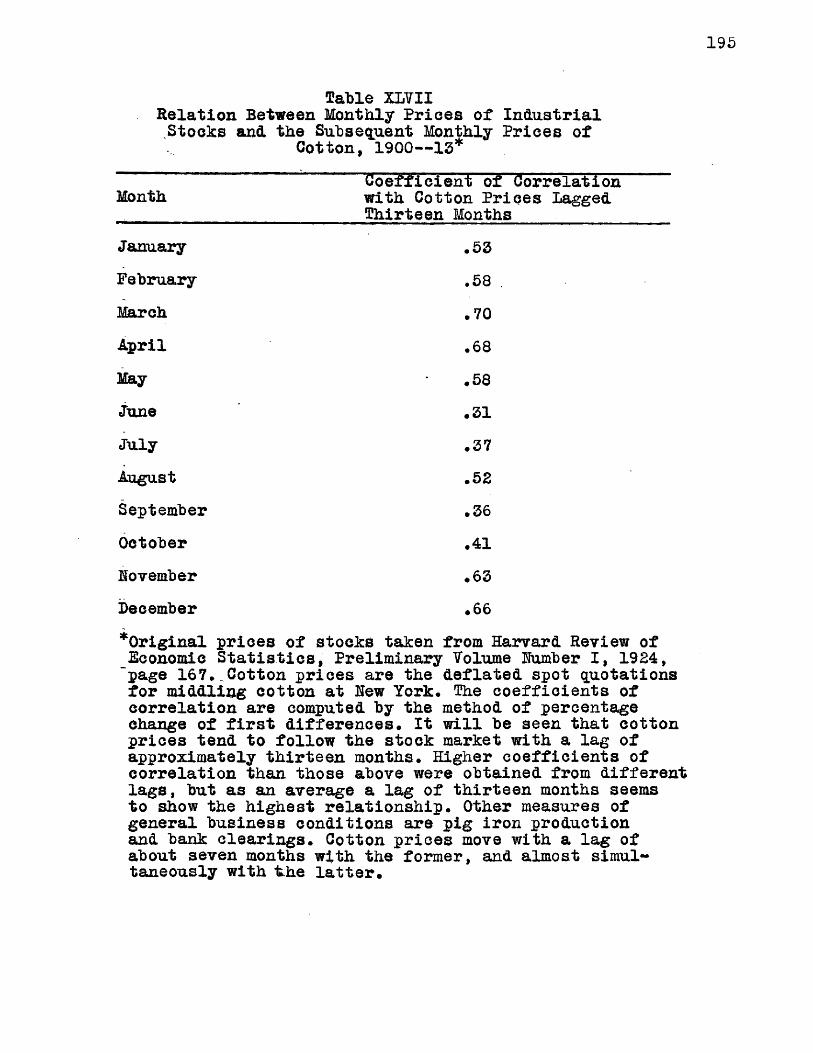
195

Table XLVIIRelation Between Monthly Prices of Industrial Stocks and the Subsequent Monthly Prices of

Cotton, 1900— 13*Coefficient of Correlation

Month with Cotton Prices Lagged„______________________Thirteen MonthsJanuary .53February .58March .70April .68May .58June .31July .37August .52September .36October .41Hovember .63December • 66^Original prices of stocks taken from Harvard Review of Economic Statistics, Preliminary Volume Humber I, 1924, page 167* Cotton prices are the deflated spot quotations for middling cotton at Hew York# The coefficients of correlation are computed by the method of percentage change of first differences. It will be seen that cotton prices tend to follow the stock market with a lag of approximately thirteen months. Higher coefficients of correlation than those above were obtained from different lags, but as an average a lag of thirteen months seems to show the highest relationship. Other measures of general business conditions are pig iron production and bank clearings. Cotton prices move with a lag of about seven months with the former, and almost simul­taneously with "the latter.

196

Table 2L7III.Relation Between Monthly Pig.Iron Production

in the United States and the Subsequent Monthly Prices of Cotton, 1900— 13*

~ Coefficient of Correlation Humber ofMonth Between Pig Iron Production Months Bag^__________ and Subsequent Cotton Prices_________ .January. .76 12February .74 8March .63 9April .59 8May .79 6June .73 12July .76 5August .75 6September .67 6October .51 8Hovember .43 9December .80 12*0riginal data on pig iron production furnished by the _Hew York State Chamber of Commerce. Cotton prices correlated axe deflated spot quotations for middling upland at Hew York. The coefficients of correlation, computed by the method of percentage change of first differences, show that cotton prices tend to follow pig iron production with a lag of approximately seven months on the average. That is, cotton prices tend toward a marked rise or.fall in normal times about seven months after pig iron production increases or decreases. The number of months lag simply means that by such a method of correlating the highest degree of relationship can be expressed. It does not mean that the relationship is not in evidence before that time.

E'­er*

3O•r-t

OJ*i— l>0PidcddPcd-pco003 0 i—IPi*r-t-PH1

0

-1

-2

t • i

Chart XXVIII* Relation Between Prices of Industrial Stocks and the Subsequent Prices of Cotton, 1900-15*

CottonStooks

*Plotted in terms of the multiples of standard deviation, with cotton lagged thirteen months* There is a tendency for cotton prices to move with the stock market ahout a year after the fluctuations in prices of stock. Another measure of general business conditions is pig iron production* Cotton prices tend to move with pig iron production with a lag of about seven months

198Cotton Acreage Harvested

Before attempting to measure the relationship existing "between acreage of cotton harvested and prices prevailing prior to planting time it is necessary to reduce the factors to a common denominator. A satisfactory expression is the percentage change of first difference in terms of the multi­ples of standard deviation of each corresponding variable. Table XLIX shows the multiples of standard deviation of cotton acreage harvested in the United States for the years 1908-24, inclusive. These multiples are the expressions of the extent to which the percentage change in acreage of each individual year deviates from the mean of the percentage changes for the entire series of years, and they are calculated by dividing the standard deviation of percentage changes into each percentage change as expressed in terms of deviation from the mean.

The reduction of individual items in a series to terms of multiples of standard deviation is a very convenient procedure in analysis involving large numbers, since the ultimate calculations are greatly facilitated. It is a method by which the extent of changes in acreage as influ­enced by prices received for the preceding crop may be readily measured, inasmuch as changes in price and acreage are ex­pressed in like terms.

LIBR

ARY, U

MVtRSi

rV OF

MARYLAND

1993*able XLIX.

Maltiples of Standard. Deviation of Cotton Acreage Harvested in the United States, 1907-24*

Year Maltiples of Standard Deviation

19071908 .1841909 - .7711910 .3131911 1.0651912 - .8001913 ' .7101914 - .3141915 - 1.9361916 1.0801917 - .6131918 .5051919 - 1.0191920 .5611921 - 1.9641922 .7231923 1.1951924 1.084*Based on original data in fable III and calculated from th© deviations of percentage changes of first differences from their mean.

200Acreage Value

The acreage of cotton planted, and. harvested, in any one year is influenced, somewhat by the acreage value of the lint of the preceding year as compared with acreage value of other crops. While cotton is the major cash crop of the South as a whole, southern farmers do have certain alternatives, and the extent to which the value of cotton per acre is less than the per acre value of crops that can be substituted is partly re­flected in a decreased subsequent acreage of cotton planted. Likewise, the prediction that a relatively high acreage value of cotton will be followed by increased plantings is about as safe as any that can be made in the field of agriculture.Stable L shows the December first farm value of cotton and the subsequent acreage of cotton harvested in the United States for the years 1882-1927, inclusive. It will be observed that there is a tendency toward direct relationship between the two series.A high value of lint tends to be associated with a relatively large acreage in the following year, and a low value tends to be associated, with a relatively low acreage.

While there is a very marked, direct relationship between December first farm value and subsequent acreage harvested, there is even greater evidence of relationship when acreage value on the basis of monthly spot quotations is compared with the extent of the next yearTs acreage. The December first farm value is not a true index to the returns actually received by the producer

201

for his cotton crop, and the quotations as of the first of the month may not reflect the true market situation in regard to price. For example, a* high or low value on December first would he reflected in a high or low value per acre, while prior to December first, when, on an average, about 53 per cent, of the current crop is marketed by farmers, the pride of lint may have been very different from the price at the beginning of December. It is, therefore, quite proper to state that the tendency toward direct relationship is greater between acreage value of lint on the basis of spot prices for the months in which most of the cotton is sold and subsequent acreage of cotton harvested than the relationship between December first value and acreage#

In Table LI are shown the multiples of standard deviation of the value of cotton per acre as expressed on the basis of the average of hew York and hew Orleans spot quotations for Middling cotton These multiples are calculated from thedeviations of percentage changes of first differences from

t

their mean. About 92 per cent, of the cotton crop of the United States is of the upland short-staple varieties, and the quo­tation for Middling, which is grade number 5, is considered by the cotton trade as a true index to the cotton price situation.

(1) The trial and error method of analysis has shown that more satisfactory results can be obtained from the average of prices at the two markets than from the prices at either hew York or hew Orleans taken singly.

The multiples of standard deviation in Table LI, therefore, reflect very satisfactorily the acreage value of cotton in terms of spot prices, the changes in purchasing power of money being ignored.

A comparison of Tables XLIX and LI will show that in most cases the plus or minus values of the multiples of standard deviation of value per acre are associated with plus or minus values of acreage of cotton harvested, indicating a direct relationship between the two factors. In most cases where plus or minus values are not associated in the two series the product of the multiples of standard deviation approach a minimum, indicating again a tendency toward direct relationship.

203

Table LFarm Value of Cotton Per Acre Based, on December

First Price and. Acreage Subsequently Harvested, 1882-1927*

Year Farm Value Per Acre December First

Acreage Harvested in Year Following Specified Year (000 omitted)

1882 $16.93 16,7781883 14.96 17,4401884 14.13 18,3011885 13.76 18,4551886 13.65 18,6411887 15.61 19,0591888 15.33 20,1751889 13.64 19,5121890 16.06 19,0591891 12.99 15,9111892 17.42 19,5251893 10.50 23,6881894 8.96 20,1851895 11.82 23,2731896 12.30 24,320189 7 12.20 24,9671898 12.63 24,3271899 13.41 24,9331900 18.58 26,7741901 12.48 27,1751902 14.85 27,0521903 19.10 31,2151904 19.33 27,1101905 21.02 31,3741906 20.26 29,6601907 19,39 32,4441908 ,17.73 30,9381909 22.55 32,4031910 25.32 36,0451911 19.08 34,2831912 23.83 37,0891913 23.26 36,8321914 14.91 31,412

(See next page)

Table L. (Continued.)

Year Farm Value Per Acreage HarvestedAcre December in Year FollowingFirst Specified Year

(000 omitted)

1915 #20.10 34,9851916 32.08 33,8411917 46.28 36,0081918 46.20 33,5661919 60.62 35,8781920 26.02 30,5091921 21.11 33,0361922 35.03 37,1231923 42.34 41,36019 2d 37.26 46,0531925 30.90 47,0871926 20.87 40,1681927. 31.20

*Value for the years 1882-1908, inclusive, tabulated and calculated from data in Yearbook of the U.S.D.A.,1919, page 590, Table 125. Value for years 1909-27, inclusive, tabulated from records of the U.S.D.A.Acreage figures are taken from Table II of this report. There is a high degree of relationship between acre value of the crop and acreage of cotton subsequently harvested, but a coefficient of correlation calculated from such relationship is not as satisfactory in formulating a predictive equation as the coefficient of correlation between deflated average spot prices at the Hew York and Hew Orleans Markets for certain months. There are several reasons for this, chief among which are the following: a high value per acre might be due to a high yield and consequent low price per pound, and a low value per acre might be the result of a low yield per acre and a price which is not correspondingly high. Then, on the technical side, the mean of percentage changes of first differences of deflated prices is less than the mean of undeflated prices, and undeflated prices are necessarily used in calculating the values per acre.

205Table LI*

Multiples of Standard. Deviation of the Value of Cotton Per Acre on the Basis of the Average of hew York and Dew Orleans Middling Spot Quotations for

Various Series of Months, 1906-23*

Year••*•

Multiples of Standard Deviation• Sept., Oct., Oct., Bov., Dec., Sept., Oct.,•* Bov., Dec. Jan., Feb. Kov., Dec.,*• Jan., Feb.,• Mar.

19061907 - .345 - .518 - .3621908 - .807 - .701 - .7221909 .511 .493 .4551910 .202 .192 .1501911 - .891 - .948 - .7911912 .107 .096 .0521913 - .028 .147 - .0951914 -1.584 -1.586 -1.3911915 .649 .860 .4281916 1.193 .953 1.024

1917 1.744 1.940 2.035

1918 .277 .016 - .007

1919 -.317 .429 .481

1920 -1.601 -1.694 -1.737

1921 -1.687 -1.462 -1.474

1922 1.325 1.292 1.624

1923 .621 .491 .331

*Based on data in Tables II, V, and XIV, and calculatedthe deviations of percentage changes of first differences from their mean.

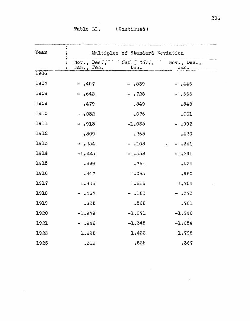
Year

19061907190819091910191119 IS19131914191519161917191819191920192119221923

Table LI. (Continued)

206

? Multiples of Standard Deviation: Nov., Dec., : Jan., Feb.

Oct., Dov., Lee.

Lov., Dec., Jan.

- .457 - .539 - .446- .642 - .728 - .666

.479 .549 .548- .032 .076 .001- .913 -1.038 - .993

.309 .268 .420- .254 - .108 . - .341-1.225 -1.553 -1.291

.399 .761 .534

.847 1.085 .9601.836 1.616 1.704

- .467 - .123 - .373.832 .562 .781

-1.979 -1.871 -1.946- .946 -1.345 -1.0541.892 1.422 1.795.319 .525 .367

207

Table LI. (Continued)

Year ; Multiples of Standard Deviation: Nov., Dec. Dec., Jan.

19061907 - .424 - .3991908 1.875 - .5791909 -1.263 .3591910 . 036 - .0561911 - .927 - .7761912 .439 .1971913 - .246 - .3981914 -1.272 -1.0211915 .608 .2051916 .955 .5671917 .448 2.1331918 - .220 - .6581919 .676 .8781920 -1.795 -1.918

1921 -1.006 - .741

1922 1.584 2.038

1923 .501 .171

£08

Undeflated Average Prices

In order to perfect the expressions of relationship "between cotton prices and acreage of cotton subsequently harvested it is necessary to carry the analysis further than the calculations of per acre values on the "basis of average monthly spot prices.While, as a normal sequence, an increased planting is subsequent to a high acreage value of lint, it is not always the case. In the years 1906, 1908, 1911, and 19£0, for example, the value of lint cotton per acre on the basis of September, October, November, and December Middling spot prices, the months during which about two-thirds of the total cotton crop is marketed by producers, was relatively high, and yet there was a decrease in the acreage of each subsequent year. The high values in these years were due to high yields, which were followed by low prices. The latter, though compensated by high yields, were the factors influencing the farmer’s decision to plant cotton, and the value per acre was of secondary importance. In the case of a low yield the value per acre on the basis of the average of September, October, November, and December spot prices and price per pound for the season are both relatively high, as in 19££ and 1923, and, for convenience, the subsequent increase in acreage planted and harvested may be considered as having been encouraged by the total returns received by the producer for his crop. As a fact, however, in economic analysis the price per pound is regarded as the determining psychological factor, since a high or low price tends in a greater

£09

degree to be followed by increased or decreased plantings than does a high or low value of lint per acre. In one case the low price per pound, despite the relatively high value per acre, is obviously the influencing factor, and in the case of the high price per pound the value per acre may be considered as an associated factor, just as the high value which is associated with low price per pound and high yield per acre.

In Table LII are the calculated multiples of standard devi­ation of average Hew York and New Orleans spot quotations for Middling cotton expressed in terms of the deviations of per­centage changes of first differences from tneir mean# They are, therefore, directly comparable with multiples of standard devi­ation of acreage in Table XLIX. ' With these prices the relation­ship to acreage of cotton subsequently harvested is more pro­nounced than the relationship between value and acreage, as shown in Tables XLIX, L, and LI. There is a stronger tendency for plus and minus values in Table LII to be associated with plus and minus values in Table XLIX, and the tendency for the products of multiples of standard deviation with unlihe signs of the two series to approach a minimum is greater than in the case of the products of similar expressions of acreage and value per acre#This indicates a greater relationship over a period of time between price of cotton per pound and acreage of the following year than between value of cotton per acre and subsequent acreage.

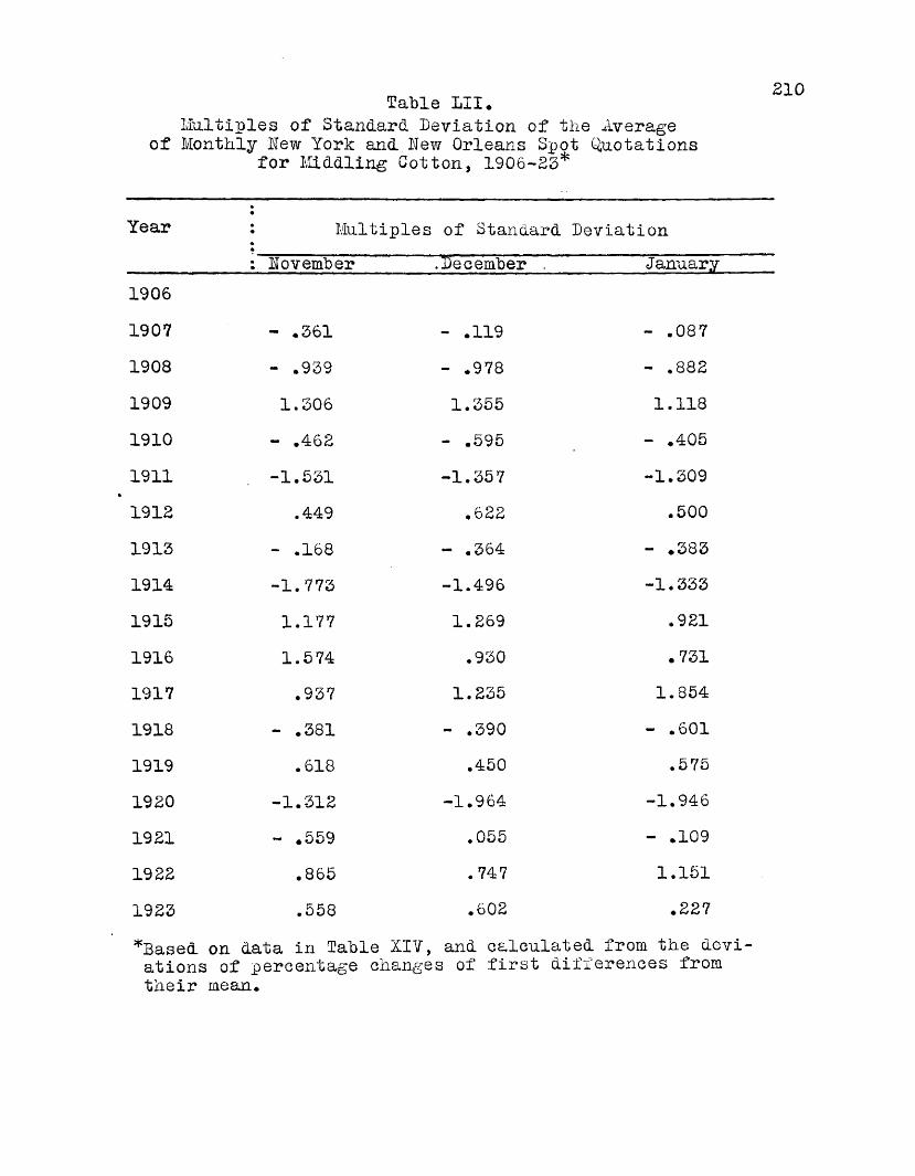
21°Table LII*Multiples of Standard Deviation of the Average

of Monthly hew York and hew Orleans Spot Quotations for Middling Cotton, 1906-23*

Year : Multiples of Standard Deviation**___________ : November .December . January19061907 - ,361 - .119 - .0871908 - .939 - .978 - .8821909 1.306 1.355 1.1181910 - .462 - .595 - .4051911 -1.531 -1.357 -1.3091912 .449 .622 .5001913 - .168 - .364 - .3831914 -1.773 -1.496 -1•3331915 1.177 1.269 .9211916 1.574 .930 .7311917 .937 1.235 1.854

1918 - .381 - .390 - .601

1919 .618 .450 .5751920 -1.312 -1.964 -1.946

1921 - .559 .055 - .1091922 .865 .747 1.151

1923 .558 • 602 .227

*Based on data in Table XIV, and calculated from the devi­ations of percentage changes of first differences from their mean.

Year

190619071908190919101911191219131914191519161917191819191920192119221923

211

Table LII. (Continued)

Multiples of Standard Deviation February ■ ■ - March

- .128 - .373

- .832 - • 6691.215 .978

- .424 - .425

-1.168 -1.008.303 • 066

- .301 - .251

-1.368 -1.190.800 .533.873 .940.490 1. 634

- .760 - .809.964 .845

-2.249 -2.105.521 .932

1.590 1.422.472 - .516

212Farm Products Index Numbers

The selection of an index number for price deflation is one of the most difficult problems confronting the economic analyst.So many indices have been published from time to time by differ­ent agencies that it is only by the method of trial and error that one can arrive at a satisfactory conclusion regarding the proper one to use in measuring the relationship between the prices of specific farm products and the acreage of the particular crop subsequently planted and harvested. The aim should be to choose that index which when used to deflate prices will give the most nearly accurate comparison of the price of the commodity in question with other commodities entering into the composite expression of price level. The index number which seems best in meeting these re­quirements to show the relationship between cotton prices and acreage of cotton planted and harvested in the subsequent year is the one published by the Bureau of Labor Statistics, computed on a 1913 base, and made by weighting the commodity prices for the years by quantities marketed in the census year 1919*

Table LIII shows the Farm Products Index Bumber for the- years 1906-26, inclusive, as published by the Bureau of Labor Statistics in T,Index Numbers of Wholesale Prices, by Years and Months, 1890 , to August, 1926”. These indices are constructed from the prices of Middling cotton, grains, livestock and poultry, beans, eggs, fruit, hay, hops, milk, peanuts, seeds, tobacco, vegetables, and wool, and a study of them indicates that they are at least as

nearly representative of farm products in regard to their re­lationships to acreages of the various crops subsequently planted as any other index number* A further study of the numbers as published by the Bureau of labor Statistics for the years since 1890 shows that farm products fluctuated below the level of all commodities from 1890 to 1908, rising slightly above all commodi­ties in 1909 and 1910. In 1911 they closely paralleled the prices of all commodities, and in 1916, with the marked increase in the general level of prices, farm products lagged behind all commodi­ties, recovering in the latter part of the year, and exceeding the prices of all commodities in 1917, 1918, and 1919. From 1920 to 1924 farm products prices fell below the prices of all commodi­ties. In 1925 they reached the level of all commodities, but fell below them in 1926. This movement of the prices of farm products in relation to the prices of all commodities is fairly representative of the actual trend of agriculture, and it con­stitutes the basis for the selection of the index number in Table LIII for cotton price deflation.

Table LIII.Index Humbers of Farm Products Prices

1906— 26*

Year Humber

1906 80.31907 86.71908 86.51909 97.01910 103.21911 93.01912 101.31913 100.01914 102.61915 103.91916 122.81917 189.61918 218.51919 230.81920 217.91921 123.71922 133.31923 141.11924 143.41925 158.11926 151.8

* "Index Humbers of Wholesale Prices, by Years and .Months, 1890 to August, 1926”, Bureau of Labor Statistics, pages 4 to 8.

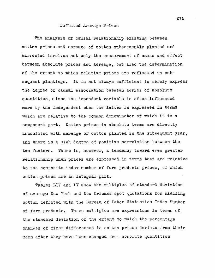
215Deflated. Average Prices

The analysis of causal relationship existing between cotton prices and acreage of cotton subsequently planted and harvested involves not only the measurement of cause and effect between absolute prices and acreage, but also the determination of the extent to which relative prices are reflected in sub­sequent plantings. It is not always sufficient to merely express the degree of causal association between series of absolute quantities, since the dependent variable is often influenced more by the independent when the latter is expressed in terms which are relative to the common denominator of which it is a component part. Cotton prices in absolute terms are directly associated with acreage of cotton planted in the subsequent year, and there is a high degree of positive correlation between the two factors. There is, however, a tendency toward even greater relationship when prices are expressed in terms that are relative to the composite index number of farm products prices, of which cotton prices are an integral part.

Tables LIV and LV show the multiples of standard deviation of average hew York and hew Orleans spot quotations for Middling cotton deflated with the Bureau of Labor Statistics Index Lumber of farm products. These multiples are expressions in terms of the standard deviation of the extent to which the percentage changes of first differences in cotton prices deviate from their mean after they have been changed from absolute quantities

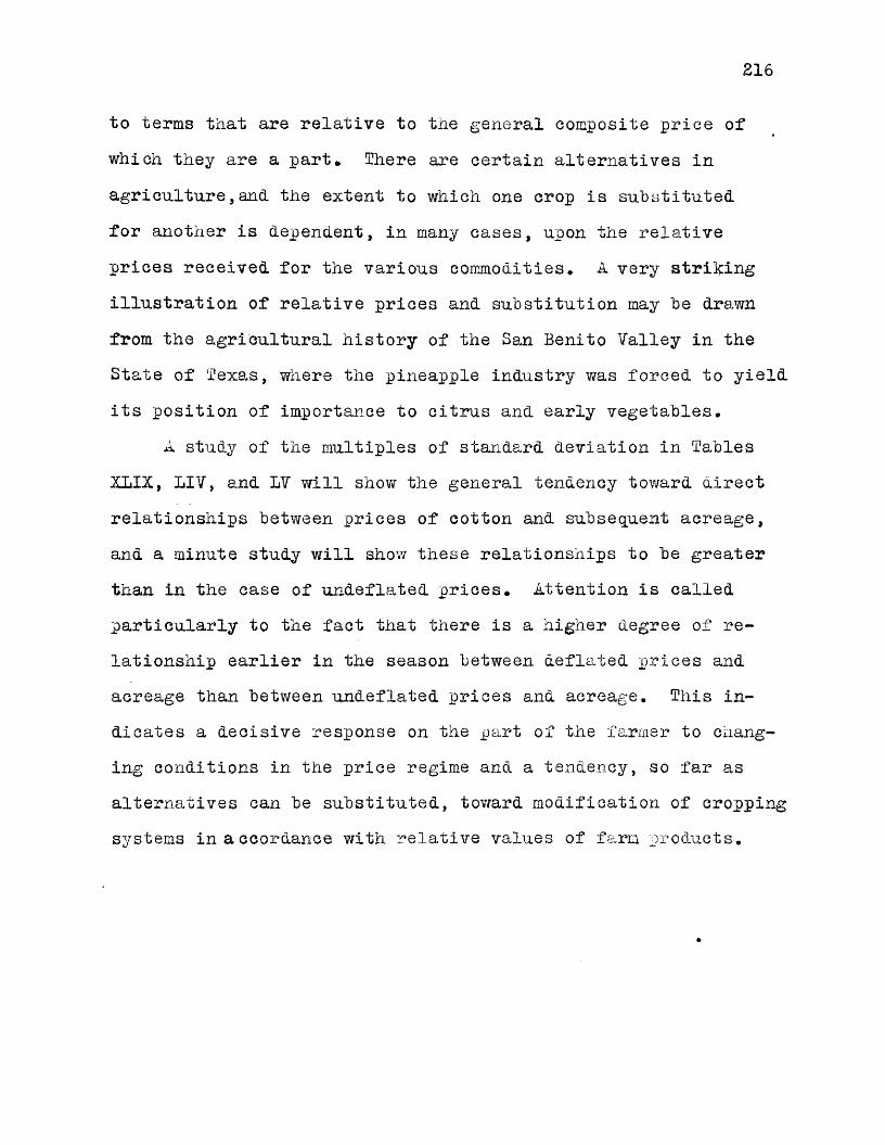
216

to terms that are relative to the general composite price of which they are a part, There are certain alternatives in agriculture,and the extent to which one crop is substituted for another is dependent, in many cases, upon the relative prices received for the various commodities. A very striking illustration of relative prices and substitution may be drawn from the agricultural history of the San Benito Valley in the State of Texas, where the pineapple industry was forced to yield its position of importance to citrus and early vegetables.

A study of the multiples of standard deviation in Tables XLIX, LIV, and LV will show the general tendency toward direct relationships between prices of cotton and subsequent acreage, and a minute study will show these relationships to be greater than in the case of undeflated prices. Attention is called particularly to the fact that there is a higher degree of re­lationship earlier in the season between deflated prices and acreage than between undef'lated prices and acreage. This in­dicates a decisive response on the part of the farmer to chang­ing conditions in the price regime and a tendency, so far as alternatives can be substituted, toward modification of cropping systems in accordance with relative values of farm products.

Table LIV.Multiples of Standard Deviation of the Average

of hew York and hew Orleans Deflated Spot Quotations for Middling Cotton, 1906-25*

Year ? Multiples of Standard Deviation: September October November

19061907 .609 - .343 - .4081908 - 1.805 - .880 - .75 71909 .738 .886 .9861910 - .442 - .301 - .4601911 - .889 -1.073 -1.1181912 - .770 - .066 .3151915 .350 .652 .0601914 - 2.352 -1.891 -1.6461915 .745 2.066 1.3121916 .711 .494 .9941917 - .801 - .219 .4251918 1.049 - .219 - .6081919 - 1.228 .343 .4961920 -

#

.392 -1.596 -1.8181921 • 366 1.575 1.8371922 - .483 .006 .7451923 .876 .568 .525

*Based on data in Table XIV, deflated with B.L.S. index number of farm products prices, 1915 base, and calculated from the deviations of percentage changes of first differ­ences from their mean.

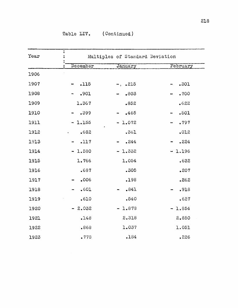
Year

190619071908190919101911191219131914191519161917191819191920192119221923

218

Table LIV, (Continued)

Multiples of Standard Deviation Deoember January February

— .115 — ,, .215 — .301- .901 - .803 - .700

1.367 .852 .622- .399 - .465 - .501- 1.155 - 1.072 - ,797

.682 • 361 .012- .117 - .244 - .224- 1.580 - 1.332 - 1.196

1.766 1.054 .632.687 .305 .207

- .006 .198 .262- .601 - .841 - .918

.610 .540 .627- 2.032 - 1.878 - 1.854

.148 2.318 2.850

.868 1.037 1.051

.778 .184 .226

219Table LV.

Multiples of Standard Deviation of the Average of New York and New Orleans Deflated Spot Quotations

for Middling Cotton for Various Series of Months, 1906-23*

Year: Sept,, : Nov.,

Oct.,Dec.

Oct., Nov., Dec.,Jan., Feb.

Nov.,Jan.,

Dec., Feb.

19061907 - .125 - .318 - .2881908 -1.041 - .887 - .7871909 1.123 .972 ♦ 8661910 - .388 - .374 - .4771911 -1.134 -1.112 -1.0271912 .139 .092 .2781913 .254 .374 - .1671914 -1.926 -1.787 -1.4071915 1.678 1.729 1.0751916 .829 .547 .4741917 - .299 - .132 - .0251918 - .246 - a444 - • 7661919 -1.035 .153 .5181920 - .810 -1.655 -1.8611921 1.811 1.937 2 • 3661922 .408 • 356 .870

1923 .763 .549 .359

*Based on original data in Table XIV, deflated with B.'index number of farm products prices, 1913 base, and calcu­lated from the deviations of percentage changes of first differences from their mean.

Table LV, (Continued)

Year ; Multiples of Standard Deviation; llov., Dec., : Jan*

Jan#, Feb.

19061907 - .279 - .2581908 - .807 - .7451909 .910 .7331910 - .460 - .4811911 -1.084 - .9241912 .888 .1741913 - .544 - .2301914 -1.442 -1.2581915 1.190 .8231916 .537 .2671917 - .131 .2311918 - .692 - .8771919 .448 .5841920 -1.803 -1.8611921 2.127 2.5631922 .758 1.0511923 .381 .210

221Coefficients of Correlation Between Cotton

Prices and Acreage of Cotton Subsequently Harvested

On the basis of the multiples of standard deviation in Tables XLIX, LI, LII, LIV, and LV, coefficients of correlation were calculated to show the extent of relationship between cotton prices and acreage of cotton harvested in the subsequent crop years. These coefficients are divided into four groups, each of which will be briefly discussed.

In Table LVI are shown the results of calculations involvingthe relationship between acreage value of cotton lint and subse­quent cotton acreage harvested. There is, as will be seen, a significant degree of positive correlation between the two factors, indicating the general tendency for cotton plantings to varydirectly with the acreage value of lint pm duced in the precedingcrop year.

The coefficients of correlation between undeflated prices and acreage are shown in Table LVII. The highest degree of re­lationship exists between February prices and acreage of the ensuing year. While the prices for the months immediately follow­ing the beginning of harvest are related in considerable degree to acreage, the greatest relationships occur between prices pre­vailing at the time planting season approaches and acreage sub­sequently planted. This would seem to involve a psychological concept as well as an economic principle, in that there is a tendency for the farmer’s intention to plant to be influenced by

2ZZ

the prices being paid for cotton at the ‘beginning of the planting season, regardless of what may actually have been received for the cotton produced in the preceding year.

Table IA/TII shows the correlations being monthly deflatedprices and acreage. These coefficients are the expressions ofrelationship on the basis of prices that have been reduced toterms which are relative to the composite expression of farm*

products prices. The highest degree of relationship exists be­tween December prices and acreage, indicating that at the end of December the relationship between prices and acreage of cotton to be subsequently planted can be fairly accurately measured and a close estimate obtained of the extent of acreage. There is a greater per cent, of the cotton crop marketed by farmers in either October or November than in December, but there is a tendency for the greater relationships to be associated with December prices because by the end of the month about two-thirds of the crop ordi­narily has been disposed of by producers, and spot prices during the months immediately following harvest are not as reflective of the cotton price regime as are prices after the size of the crop is more nearly definitely known to the cotton trade. This is be­cause prices are largely dex^endent upon the size of the cotton

cropTable LIX shows the coefficients of correlation between

average prices for various series of months and acreage of cotton subsequently planted and harvested. In a way these coefficients

ZZ2>

are tributary to those in Table LVIII, since the degree of relationship between production and price immediately follow­ing the beginning of harvest tend to be offset by the more direct relationships between production and price after the former is more nearly definitely known. This is an important factor because the extent to which production and price of the current harvest year are related will tend to be reflected in the acreage planted and harvested in the next crop year. Any factor which diminishes the expression of relationship between production and prices will likewise tend to diminish indirectly the relationship between price and acreage.

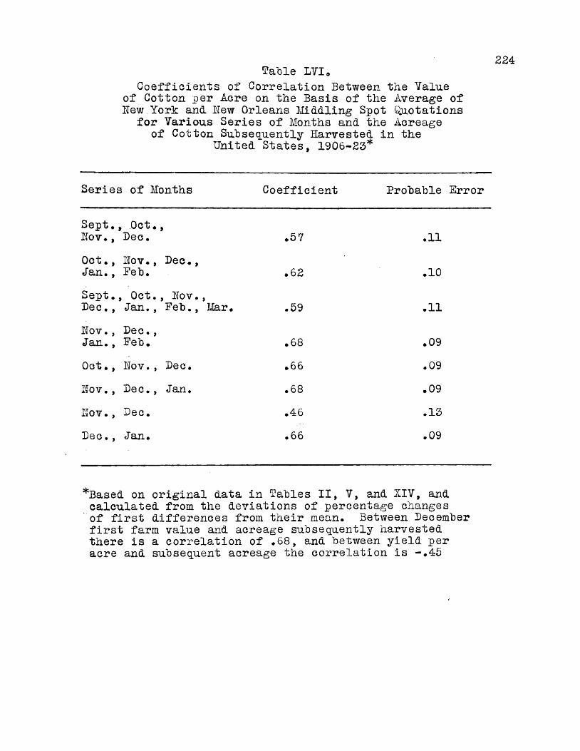
224£able LVI.

Coefficients of Correlation Between the Value of Cotton per Acre on the Basis of the Average of Hew York and Hew Orleans Middling Spot Quotations

for Various Series of Months and the Acreage of Cotton Subsequently Harvested in the

United States, 1906-23*

Series of Months Coefficient Probable Error

SeptHov.

., Oct.,, Dec. .57 .11

Oct.Jan.

, Hov*, Dec.,, Feb. .62 .10

SeptDec.

., Oct., Hov.,, Jan., Feb., Mar. .59 .11

Hov.Jan.

, Dec.,, Feb. . 68 .09

Oct. , Hov., Dec. .66 .09Hov. , Dec., Jan. .68 .09Hov. , Dec. .46 .13Dec., Jan. .66 .09

*Based on original data in tables II, V, and XIV, and calculated from the deviations of percentage changes of first differences from their mean* Between December first farm value and acreage subsequently harvested there is a correlation of *68, and between yield per acre and subsequent acreage the correlation is -*45

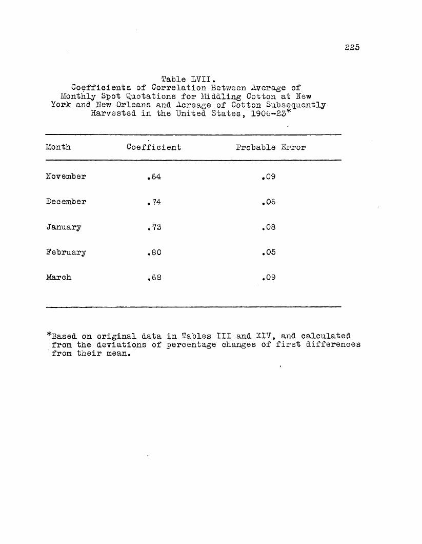
225

Table LVII.Coefficients of Correlation.Between Average of

Monthly Spot Quotations for MiIdling Cotton at Hew York and Hew Orleans and Acreage of Cotton Subsequently

Harvested in the United States, 1906-23*

Month Coefficient Probable Error

Hovember .64 .09

December .74 .06

January .73 .08

February o00• .05

March .68 .09

*Based on original data in Tables III and XIY, and calculated from the deviations of percentage changes of first differences from their mean.

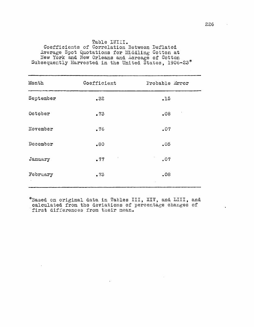
226

Table 1VIII.Coefficients of Correlation Between Deflated.

Average Spot Quotations for Middling Cotton at Hew York and Hew Orleans and Acreage of Cotton

Subsequently Harvested in the United States, 1906-23*

Month Coefficient Probable Error

September .32 .15

October .73 .08

Hovember .76 .07

December oCO. • 05

January .77 *07

February .73 00o•

*Based on original data in Tables III, HIV, and LIII, and calculated from the deviations of percentage changes of first differences from tneir mean.

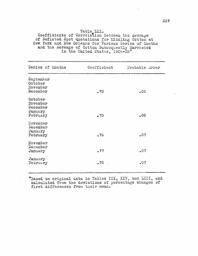
227

Table LIZ.Coefficients of Correlation Between the Average of Deflated Spot Quotations for Middling Cotton at

Lew York and Lew Orleans for Various Series of Months and the Acreage of Cotton Subsequently Harvested

in the United States, 1906-25*

Series of Months Coefficient Probable Mrror

SeptemberOctoberLovemberDecember .73 . o CO

OctoberLovemberDecemberJanuaryFebruary .73 .08LovemberDecemberJanuaryFebruary .76 .07LovemberDecemberJanuary .77 .07JanuaryFebruary .75 . .07

*Based on original data in Tables III, XIV, and IIII, and calculated from the deviations of percentage changes of first differences from their mean.

228Acreage Estimates

The making of acreage estimates involves the calculation of regression of acreage on price, which, varies in magnitude with the coefficient of correlation. A high value of the latter is associated with a relatively high value of regression, indi­cating the possibility of more nearly accurate estimates than could he made from a low coefficient of correlation and a correspondingly low regression coefficient. This merely involves the concept that deviations of actual acreages from the esti­mated acreages tend to a minimum as the size of the numerical egression of regression increases in magnitude.

In Table LX are shown the actual percentage changes in acreage of cotton harvested in the years 1908-24, inclusive, and the percentage changes as estimated from the expression of re­lationship between December deflated spot quotations for Middling cotton at hew York and hew Orleans and the acreage of cotton harvested in the subsequent crop year. It will be seen that for the period as a whole the estimated percentage changes and actual percentage changes are identical, indicating that over a series of years the December prices may be relied upon as a basis for estimating percentage changes in subsequent acreages.

In Table LXI the actual acreages and the acreages as esti­mated from the estimated percentage changes in Table LX are compared. ,0n the whole the estimated acreage was 4.97 per cent.

229

less than actual acreage, This close approximation is significant, since a difference as great as 2,000,000 acres is equivalent to only about three-fifths of a million bales of lint. When it is realized that these estimates are made before the cotton crop is planted, and one year prior to the report on final ginnings, their degree of accuracy assumes even greater significance.

Another way of making acreage estimates is by the ”ratio method”. These are made on the assumption that the size of the current yearTs crop is reflected in price, which in turn is reflected in acreage planted and harvested. The estimate for any one year is made by multiplying the production ratio by the acreage ratio. For the twenty-seven year period, 1901-27, inclusive, as shown in Table LXII, the acreage as estimated was 2,63 per cent, less than the actual acreage harvested in the subsequent crop year. This difference of 2.63 per cent, in acreage estimates is equivalent to only 2.37 per cent, of the total production as measured by the average for the period 1901-27, inclusive.

Chart XXIX shows graphically the actual and estimated percentage changes in cotton acreage harvested for the years 1919-24 as expressed in terms of multiples of standard devia­tion. This Chart is based on data in Table LX. The estimated changes, as will be observed, deviate only slightly from actual*

230

Table LX.The Actual Percentage Changes in Cotton Acreage Harvested, in the United States and the .Changes as Estimated, 1908-24*

Year Actual Percentage Estimated PercentageChange Change

1908 3.62 1.211909 - 4.64 - 4.331910 4.74 11.691911 11.24 - .781912 - 4.89 - 6.131913 8.18 6.851914 - .69 1.211915 -14.72 - 9.131916 11.37 14.521917 - 3.27 6.891918 6.40 1.991919 - 6.78 - 2.221920 6.89 6.351921 -14.96 -12.331922 8.28 3.081923 12.37 8.171924 11.41 7.53

Average 2.03 2.03

*Estimates are made on the basis of relationship between the average of Hew York and Hew Orleans December spot quotations for Middling cotton, deflated with B.L.S. index number of farm products prices, 1913 base, and subsequent acreage of cotton harvested. In making the estimates the following formula was used: y = Ay minusbAx plus bx, in which y is the percentage change in acreage, Ay the average of the percentage change in acreage, x the percentage change in price, Ax the average of percentage change in price, and b the coefficient of regression of acreage on price, determined by dividing the standard devi­ation of the acreage series by the standard deviation of the price series and then multiplying by the coefficient of correlation between price and acreage subsequently harvested.

221

Table LXI.The Actual Acreage of Cotton Harvested. .in the United States and the Acreage

as Estimated, 1908-24*

Year Actual Acreage Estimated Acreage(000 omitted) (000 omitted)

1908 22,444 51,6901909 20,958 51,0591910 52,405 54,5541911 56,045 52,1501912 54,285 55,8551912 57,089 56,6511914 56,852 57,5571915 51,412 55,4691916 54,985 55,9 751917 55,841 57,5951918 56,008 54,5141919 55,566 55,2081920 55,878 55,6971921 50,509 21,4541922 55,056 51,4491925 57,125 55,7551924' 41,260 59,918

Average 56,415 54,605

^Estimates are made on the basis of relationship between the average of Hew York and Hew Orleans December spot "quotations for Middling cotton, deflated with B.L.S. index number of farm products prices, and subsequent acreage of cotton harvested. On an average the acreage as estimated was 4.9 7 per cent, less than the actual acreage. Slight variations are negligible, since a difference as great as 2,000,000 acres is equivalent to only approximately three-fifths of a million bales of lint. These facts are noteworthy when it is realized that estimates of harvested acreage are made one year in advance.

Year

1900190119021905190419051906190719081909191019111912191319141915191619171918191919201921192219231924192519261927

232

Table LXII.Production and Acreage Ratios of Cotton Harvested in the United States, 1900-27*

Production Ratio (per cent, five year average ending with specified year is of

specified year)

Acreage Ratio (per cent, acreage of specified year is of acreage of pre­

ceding year)

88.897.890.8 98.477.3

100.481.897.985.4

112.999.377.091.389.081.9

116.0 113.7113.3 108.2113.994.9

152.4 119.3 108.182.573.069.598.4

102.5107.4101.599.5

115.4 86.8

115.794.5

109.4 95.4

104.7 111.295.1

108.299.385.3

111.4 96.7

106.493.2

106.985.0

108.3112.4111.4 111.3 102.285.3

(See following page)

233

Table EXXI. (Continued)

SjrThe estimate of acreage for any subsequent year is made by multiplying the acreage of the specified year by the product of the production and acreage ratios. For the twenty-seven year period, 1901-27, inclusive, the total actual acreage harvested was 921,420,000, an average of34.126.000 acres per year. For the same period the total estimated acreage harvested was 896,637,000, an average of33.209.000 acres per year. The difference is 917,000, meaning that the acreage as estimated was 2,63 per cent, less than the actual acreage harvested one year hence.At 152 pounds per acre, which is both the ordinate of the line of least squares and the yield per acre for the year 1927, the difference of 917,000 acres represents 291,598 bales of 478 pounds, or 2.37 per cent, of the total cotton crop as measured by the average production for the years 1901-27, inclusive. In other words, knowing the acreage and production of cotton for any specified year, it was possible to estimate by the ratio method, one year in advance, within 2.63 per cent, of the acreage harvested during the subsequent year, and within 2.37 per cent, of the production of cotton for the same subsequent year.

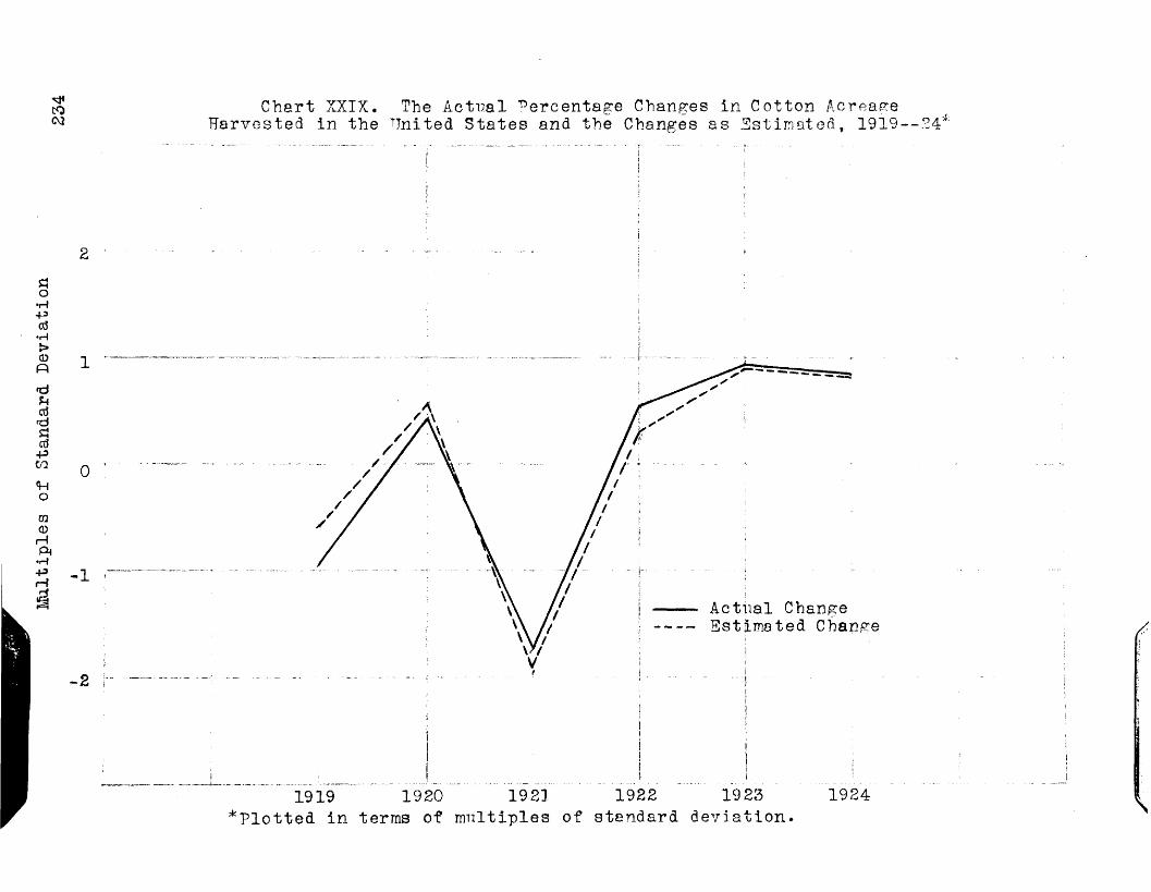
Multiples

of Standard

Devi

atio

n

tg(xi

Chart XXIX. The Actual Percentage Changes in Cotton AcreageHarvested in the Hnited States and the Changes as Estimated,

2

Actual Change Estimated Change

[

1919 1920 1921 1922 19 23 1924*Plotted in terms of multiples of standard deviation.

235Yield of lint Cotton Per Acre

In the analysis involving determination of relationships "between various weather factors and yield of lint cotton per acre two representative counties in Sorth Carolina, Wake and Cumberland, were selected. These counties are situated in different parts of the cotton area of the State, and are con­sidered as being representative of the status of cotton production in the two areas*

Table LXIII shows the yield per acre of lint cotton in the counties of Wake and Cumberland* luring the twenty-three year period, 1904-26, inclusive, the yields of Wake County were above the State yields in seven different years, and were the same asthe State yields in one year, 1909, when the yield for both County

\and State was 210 pounds, luring the same twenty-three year period the yields of Cumberland County were above the State yields in twelve different years. These facts indicate that during these years there was a decided tendency for Wake County yields to fall below State yields, and a slight tendency for Cumberland County yields to exceed the yields of the State as a whole.

A further analysis of the data in Table 1XIII shows that during the years 1904-27, inclusive, the trend of Wake County yields was upward at the rate of 4.3 pounds per year, while the yearly trend of yields in Cumberland County was upward at the rate of only 1.2 pounds These differences in trend of yields

(1) Ordinate of the straight line of least squares.

illustrate a further dissimilarity in the status of cotton production in the two counties, which, together with the relative magnitudes of yields as compared with those of all the counties taken collectively, has significance in that the aim has been in this study to select areas of production which are unlike in acreage yields*

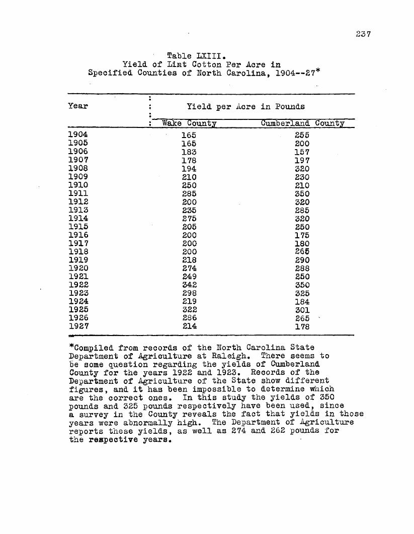
23 7

Table LXIII.Yield, of lint Cotton Per Acre in

Specified Counties of North Carolina, 1904— £7*

Year : Yield per Acre in Pounds: Wake County Cumberland County

1904 165 2551905 165 2001906 183 1571907 178 1971908 194 3201909 210 2301910 250 2101911 285 3501912 200 3201913 235 2851914 275 3201915 205 2501916 200 1751917 200 1801918 200 2651919 218 2901920 274 2881921 249 2501922 342 3501923 298 3251924 219 1841925 322 3011926 286 265 '1927 214 178

^Compiled from records of the North Carolina State Department of Agriculture at Raleigh. There seems to be some question regarding the yields of Cumberland County for the years 1922 and 1923. Records of the Department of Agriculture of the State show different figures, and it has been impossible to determine which are the correct ones. In this study the yields of 350 pounds and 325 pounds respectively have been used, since a survey in the County reveals the fact that yields in those years were abnormally high. The Department of Agriculture reports these yields, as well as 274 and 262 pounds for the respective years.

238

Weather Factors

The weather data used in this study were tabulated from the official records of the United States Weather Bureau at Raleigh, North Carolina. Daily numerical expressions of sun­shine, precipitation, and temperature were compiled and summated by monthly, semi-monthly, and weekly periods. The totals of the various factors for different ranges of time were then correlated with subsequent yields of lint cotton per acre.

Table LXIY shows the relative weights of May, June, and July precipitation and mean temperature for Cumberland County as cal­culated by the method of determinants from secular trend resid­uals* The concept involved in these calculations is that the numerical expressions of relative importance represent the extent to which each of the six factors, taken collectively, is related to yields per acre* Table LXY shows the relative weights of May, June, July, and August precipitation, mean, maximum, and minimum temperature, and sunshine for Cumberland County. These weights, like those in Table LXIY, show the relative importance of the various factors when the entire group is considered together, and they involve the principle that secular trend residuals of various weather conditions are associated in varying degrees with the current season’s production of cotton. This is evidenced by the tendency for the summation of the products of weights and residuals to equal the residuals of yield per acre.

239

In calculating the relationships between weather factors and yield of cotton in Wake County and a t the North Carolina Agricultural Experiment Station the actual data were used instead of relative weights. For convenience, however, the actual numerical expressions of the various factors were re­duced to multiples of standard deviation in terms of deviation of percentage changes of first differences from their mean. These multiples were then correlated with similar expressions of yield of lint cotton. This method of reducing actual data to multiples of standard deviation has the advantages of re­ducing numerical magnitudes and of removing most of the trend from the series correlated*

240

Table LXIV•Relative Weights-of Six Weather Factors When Correlated With Subsequent Yield of Cotton

Per Acre in Cumberland County, H.C., 1904-24*

Weather Factor Weight

May Precipitation (A) -16*84

June Precipitation (B) - .37

July Precipitation (C) - 4.64

May Mean Temperature (E) 9.30

June Mean Temperature (F) 13.20

July Mean Temperature (G ) 17.07

*The equations for determining the weights of the various faetors are formulated and solved by the method of determinants*

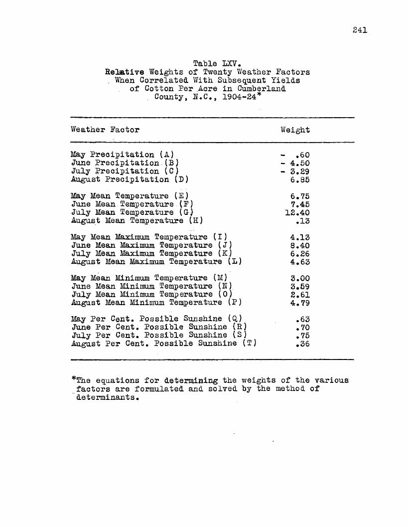
241

Table LXV.Relative Weights of Twenty Weather Factors . When Correlated With Subsequent Yields

of Cotton Per .Acre in Cumberland . County, R.C., 1904-24*

Weather Factor Weight

May Precipitation (A) - .60June Precipitation (B) - 4.50July Precipitation (C) - 3.29August Precipitation (D) 6.85Miay Mean Temperature (E) 6.75June Mean Temperature (F) 7.45July Mean Temperature (Gj 12.40August Mean Temperature (H) .13May Mean Maximum Temperature (I) 4.13June Mean Maximum Temperature (J) 8.40July Mean Maximum Temperature (Kj 6.26August Mean Maximum Temperature (L) 4.63May Mean Minimum Temperature (M) 3.00June Mean Minimum Temperature (N) 3.59July Mean Minimum Temp erature (0) 2.61August Mean Minimum Temperature (P) 4.79May Per Cent. Possible Sunshine (Q.) .63June Per Cent. Possible Sunshine (R) .70July Per Cent. Possible Sunshine (S.) .75August Per Cent. Possible Sunshine (T) .36

*The equations for determining the weights of the various _factors are formulated and solved by the method of det e rmi nant s•

242

Measures of CorrelationWeather Factors and. Yield, of lint Cotton at the Worth Carolina Experiment Station.

It is obvious, of course, that there must be some relation between weather factors and. subsequent yield of cotton, faking all conditions collectively, some react favorable, some unfavor­ably, and some show no relationship at all. in attempt has been made to show the degree of correlation between various factors for different periods of time and the final yield of cotton lint. In the calculation of these expressions of correlation, each factor has been taken separately, and the degrees of relation­ship are shown on that basis.

fables H V I to L2X, inclusive, show the expressions of re­lationship between precipitation, sunshine, and temperature and yield of cotton on experimental plots at the Worth Carolina Agricultural Experiment Station. It will be observed that for certain well-defined periods there is a very high degree of re­lationship between weather and yield, while for other periods the relationship is negligible. Between precipitation for the months of July and August and subsequent yield of lint, as shown in fable LXVI, there is a correlation of .96, while for shorter periods the coefficients of correlation range from .46 to .86.It is interesting to observe the high degree of relationship between precipitation for weekly periods and yield. In Table LXYII there will be seen a coefficient of correlation as high as .81 between sunshine for the week of June 25th to July 1st

and subsequent yield. Similar coefficients calculated for the fourteen day period, June 25th to July 8th, and for the seven day period, July 2nd to July 8th, indicate that a high percentage of sunshine during these periods is favorable to high production* In this connection the reader will observe in Table LXVI that for the same fourteen day period there is a high degree of re­lationship between precipitation and yield, indicating further that bountiful rainfall followed by a high percentage of sunshine from June 25th to July 8th is favorable to growth of plant and yield of lint. The calculated expressions of relationship be­tween temperature and yield are shown in Tables L O T H , LXIX, and LXX, There are varying degrees of association between tem­perature and subsequent yield, and in interpreting them the reader is to understand that they are based on conditions which, in analysis, must be assumed to be more or less static, or to have undergone compensating changes.

Tables LXIX and LXX show an appreciable degree of positive relationship between high temperatures and yield from June 25th to July 1st, and in Tables LXVI and LOTI it will be observed that when bountiful rainfall and a high percentage of sunshine are associated directly with temperature during this period there is a tendency toward an associated subsequent high yield of cotton. A further study of Tables LOI, LXIX, and LXX will show that there is a tendency for precipitation and temperature in late July and early August to be conducive to lint growth.

244

There are many variations in degree of association between single weather factors and yield of cotton, as well as almost innumerable multiple relationships. The question of forecasting cotton production resolves itself into the problem of determining the extent of variation in response to weather conditions, time of planting, ravages of pests, and cultural practices, and this can best be done by the par method, which takes into consider­ation those conditions not subject to accurate numerical measurement •

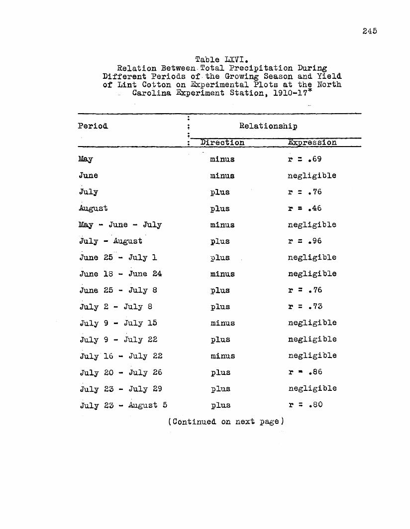
245

fable LXVI.Relation Between lotal Precipitation Boring

Different Periods of the Growing Season and Yield of Lint Cotton on Experimental Plots at the Rorth

Carolina Experiment Station, 1910-17*

Period : Relationship: Direction Expression

May minus r = .69June minus negligibleJuly plus <£>?>-.ii&

August plus .IIU

May - June - July minus negligibleJuly - August plus r = .96June 25 - July 1 plus negligibleJune 18 - June 24 minus negligibleJune 25 - July 8 plus r = .76July 2 - July 8 plus r = .73July 9 - July 15 minus negligibleJuly 9 - July 22 plus negligibleJuly 16 - July 22 minus negligibleJuly 20 - July 26 plus CO.1u

July 23 - July 29 plus negligibleJuly 23 - August 5 plus H ti » 00 o

{Continued on next page)

246

£able LXVI. (Continued)

•

Period :••

Relationship: Direction ISxpression

August 6 - August 12 plus negligibleAugust 13 - August 19 plus negligibleAugust 20 - August 26 minus negligibleAugust 27 - September 2 plus negligible

*In calculating the degree of relationship, all factors except precipitation have been ignored* Hence, in inter-

preting the expressions it is to be understood that other factors in conjunction might react either favorably or unfavorably on subsequent yield.

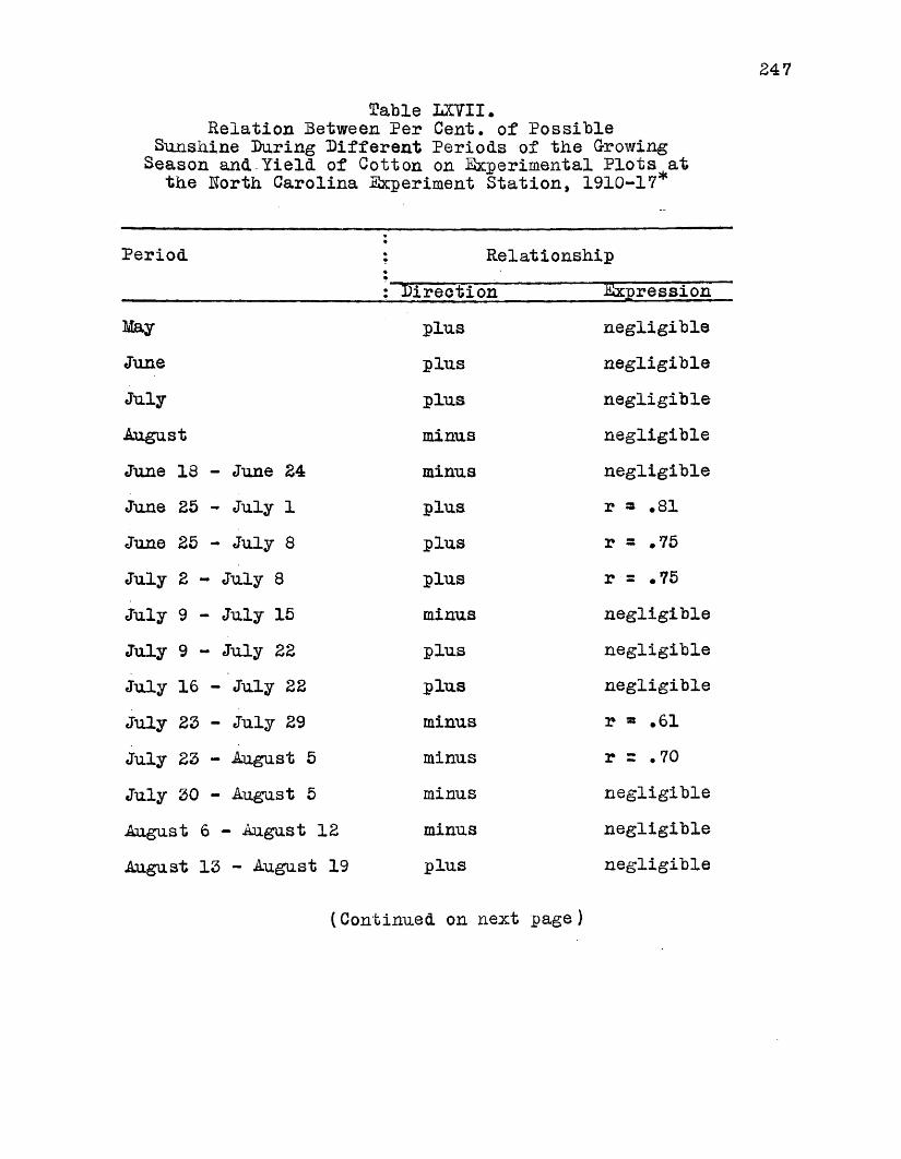
Table LXVTI.Relation Between Per Cent, of Possible

Sunshine During Different Periods of the Growing Season and-Yield of Cotton on Experimental Plots at

the Rorth Carolina Experiment Station, 1910-17

Period ; Relationship: direction Expression

May plus negligibleJune plus negligibleJuly plus negligibleingust minus negligibleJune 18 - June 24 minus negligibleJune 25 - July 1 plus 11 • CO W

June 25 - July 8 plus r = .75July 2 - July 8 plus r = .75July 9 - July 15 minus negligibleJuly 9 - July 22 plus negligibleJuly 16 - July 22 plus negligibleJuly 23 - July 29 minus r « .61July 23 - August 5 minus r = .70July 30 - August 5 minus negligibleAugust 6 - August 12 minus negligibleAugust 13 - August 19 plus negligible

(Continued on next page)

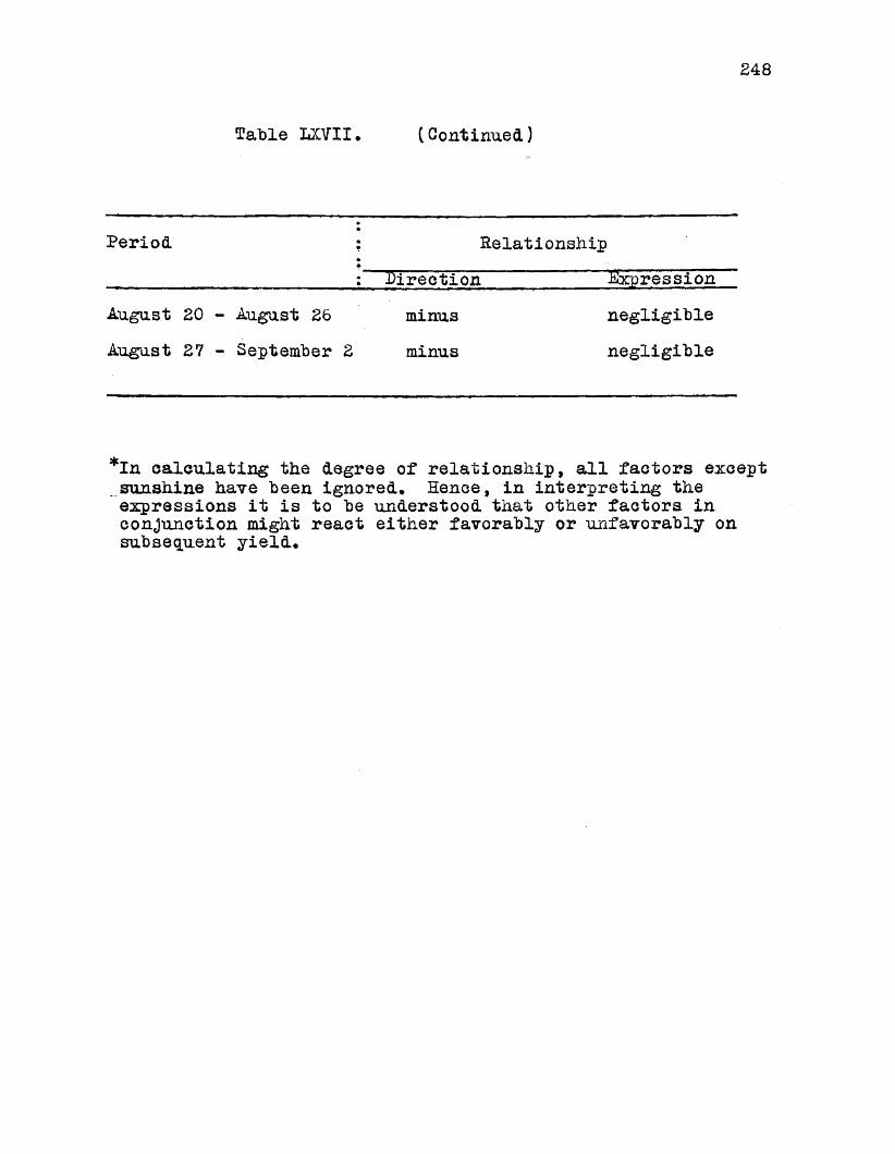
£48

Table IXVII* (Continued.)

Period RelationshipDirection Expression

August 20 - August 26 minus negligibleAugust 27 - September 2 minus negligible

*In calculating the degree of relationship, all factors except .sunshine have been ignored* Hence, in interpreting the expressions it is to be understood that other factors in conjunction might react either favorably or unfavorably on subsequent yield.

249

Table LXVTII.Relation Between Mean Temperature During Different Periods of the Growing Season and Yield of Lint Cotton on Experimental Plots at the Horth Carolina Experiment Station,

1910-17*

*

Period ;*•

Relationship•• Direction Expression

May plus negligibleJune plus r s .50July plus negligibleAugust minus negligibleJune 18 - June 24 plus r a .76June 25 - July 8 minus r = ,53July 9 - July 15 plus r s .53July 16 - July 22 minus negligibleJuly 23 - August 5 plus negligibleAugust 6 - August 12 plus r = .72August 13 - August 19 minus negligibleAugust 20 - August 26 minus r » .50August 27 - September 2 minus negligible

*In calculating the degree of relationship, all factorsexcept mean temperature have been ignored. Hence, in interpreting the expressions it is to be understood that other factors in conjunction might react either favorably or unfavorably on subsequent yield*

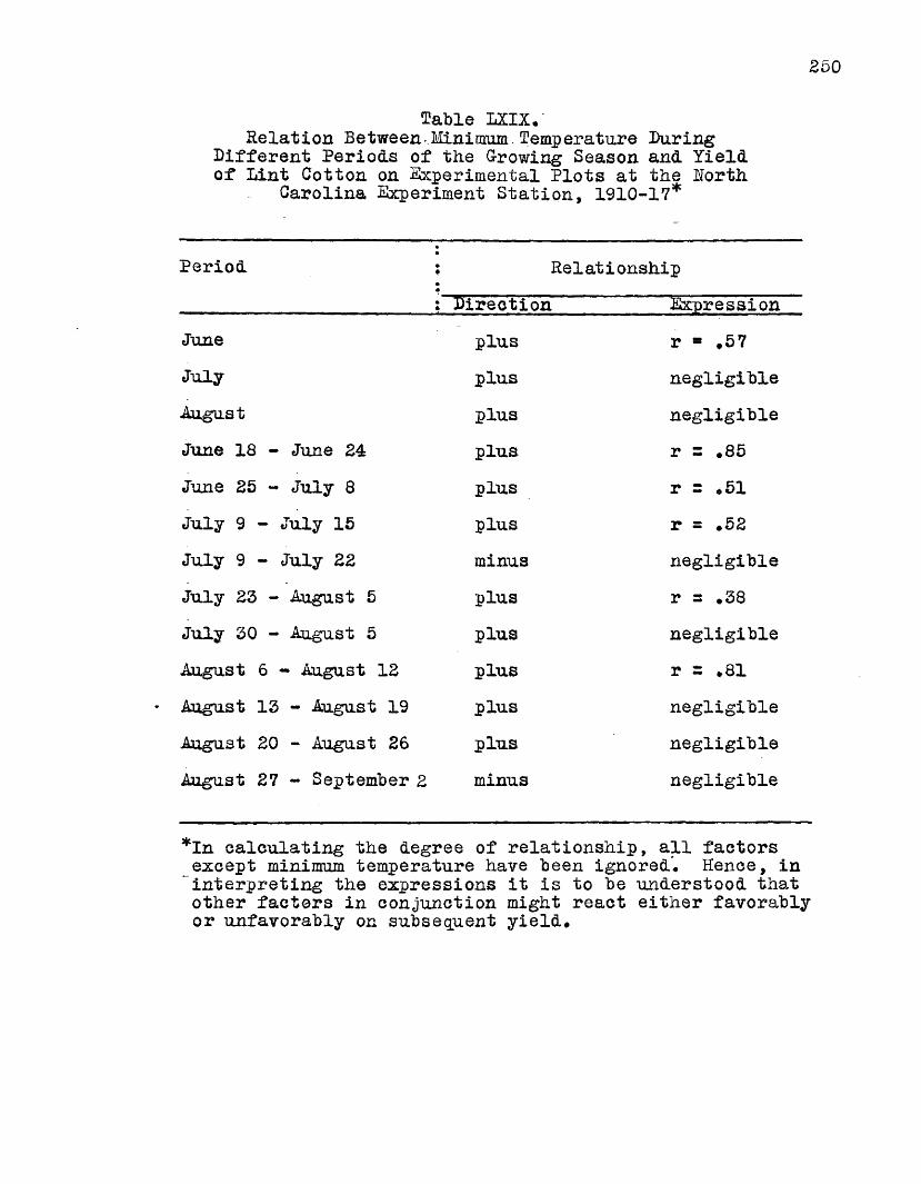
250

Cable LXIX#Relation Between-Minimum.Temperature During

Different Periods of the Growing Season and Yield of Lint Cotton on Experimental Plots at the Horth

Carolina Experiment Station, 1910-17*

*•

Period ;•«

Relationship♦* Direeti on Expression

June plus r « #57July plus negligibleAugust plus negligibleJune 18 - June 24 plus r = .85June 25 - July 8 plus r = #51July 9 - July 15 plus r = .52July 9 - July 22 minus negligibleJuly 23 - August 5 plus r = #38July 30 - August 5 plus negligibleAugust 6 - August 12 plus r = .81August 13 - August 19 plus negligibleAugust 20 - August 26 plus negligibleAugust 27 - September 2 minus negligible

*In calculating the degree of relationship, all factors except minimum temperature have been ignored’# Hence, in interpreting the expressions it is to be understood that other factors in conjunction might react either favorably or unfavorably on subsequent yield#

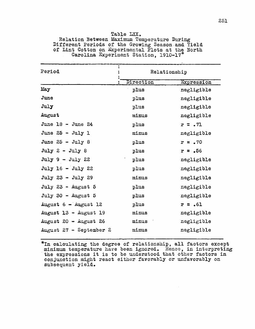
251

Table LXX.Relation Between Maximum Temperature During

Different Periods of the Growing Season and Yield of Lint Cotton on -Experimental Plots at the Horth

Carolina Experiment Station, 1910-17*

Period Relationship: Direction Expression

May plus negligibleJune plus negligibleJuly plus negligibleAugust minus negligibleJune 18 - June 24 plus r - .71June 25 - July 1 minus negligibleJune 25 - July 8 plus r = *70July 2 - July 8 plus r = .56July 9 - July 22 plus negligibleJuly 16 - July 22 plus negligibleJuly 23 - July 29 minus negligibleJuly 23 - August 5 plus negligibleJuly 30 - August 5 plus negligibleAugust 6 - August 12 plus r a .61August 13 - August 19 minus negligibleAugust 20 - August 26 minus negligibleAugust 27 - September 2 minus negligible

*In calculating the degree of relationship, all factors except minimum temperature have been ignored. Hence, in interpreting the expressions it is to be understood that other factors in conjunction might react either favorably or unfavorably on subsequent yield*

252

Weather Factors and Yield of Cotton in Wake County, North Carolina.

fhe results of analysis showing relationship "between weather factors and yield of lint cotton in Wake County, North Carolina, are given in fables LXXI to LZXYI, inclusive. Ex­pressions of relationship between mean temperature and yield and maximum temperature and yield are shown for two periods, 1900-17 and 1900-24. In the case of precipitation and minimum temperature all analysis apply to the shorter period, 1900-17. fhese tables are self-explanatory, and it will be observed that there are varying degrees of relationship between the different factors and subsequent yield. Bountiful rainfall and high maximum temperature during the first half of July tend to be favorable to yield, while during the latter half of the month excessively high temperatures when associated with high precipi­tation react unfavorably, This latter tendency is probably due to the detrimental effects of high temperatures coming immedi­ately after heavy rainfall. High temperature and rainfall when associated during the second and third weeks of August tend to be favorable to yield of lint. This relationship, as well as in the case of the first half of July, is due mainly, perhaps, to frequent showers of light rainfall. A*heavy,dashing rain when followed immediately by excessively high temperature is particu­larly detrimental to cotton at certain periods, and it is such conditions as these which the par method of estimates takes into consideration, but which cannot be measured by regression.

253

The expressions of relationship in Tables LXXI to LXXVI are given to impress the reader with the fact that even though there must necessarily be some eausal association between weather factors and yield of cotton,there are at the same time innumerable counteracting climatic influences and certain re­versals in response which cannot be measured in rigid mathematical equations. In calculating multiple regression there is a ten­dency for positive relationship between precipitation and yield to be offset by both excessively low and high temperatures. At the same time, positive correlation between certain other factors and yield for one period may be offset by a reversal of response during another period. An illustration of this condition may be drawn from the relationship between July precipitation and sub­sequent yield of lint in Cumberland County, where from 1908 to 1915 there was a tendency for high rainfall to be followed by low yields, and from 1916 to 19S4 the tendency was for rainfall and yield to be directly associated. A similar illustration may be taken from the data representing Wake County. From 1907 to 1924 there was a direct correlation between precipitation and yield for the period of August 6th to August 19th, inclusive, taking the series of years as a whole, but for individual years a high precipitation and a high yield were not always directly associated. On the contrary, there was much inverse relation­ship. In 1904, for example, the rainfall for the period was about one and one-half inches, and the yield of lint that year

254

was 165 pounds per acre, while in 1905 a precipitation of six and one-half inches was followed by an ultimate yield of 165 pounds, just as in 1904♦ Similar conditions occurred in 1915, 1918, and 1919, when in the former year a precipitation of less than two-tenths of an inch was followed by a yield of 205 pounds of lint per acre, while a precipitation of one and seven-tenths inches in 1918 was associated with a yield of 200 pounds, and in 1919 the low precipitation of six-tenths of an inch was followed by the high yield of 218 pounds per acre* ©iese examples are presented to show how the effects of specific weather factors are counteracted by other factors, with the result that multiple coefficients of correlation cannot be used as satisfactorily as condition pars for the basis of making production estimates*

Table LXXI.Relation Between Total Precipitation Poring

Different Periods of the Growing Season and Yield of Lint Cotton Per Acre

in Wa&e County, H.C., 1900-17*

Period : Relationship: Pirection Expression

June 4 - June 24 minus r = .37June 4 - July 1 minus negligibleJune 25 - July 2 minus negligibleJune 11 -- July 5 minus r = .27June 18 - July 1 minus negligibleJune 25 - July 29 plus r = .38June 25 - August 5 plus negligibleJuly 2 - July 8 minus negligibleJuly 2 - July 10 plus r s .57July 2 - July 22 plus r = .35July 2 - July 29 plus r z .41July 2 - August 5 plus r = .43July 9 - July 15 minus negligibleJuly 9 - July 22 plus r = .32July 9 - August 5 minus r = .35July 9 July 29 plus negligibleJuly 16 - July 22 minus r = .37July 16 - July 29 minus r = .34

(Continued on next page)

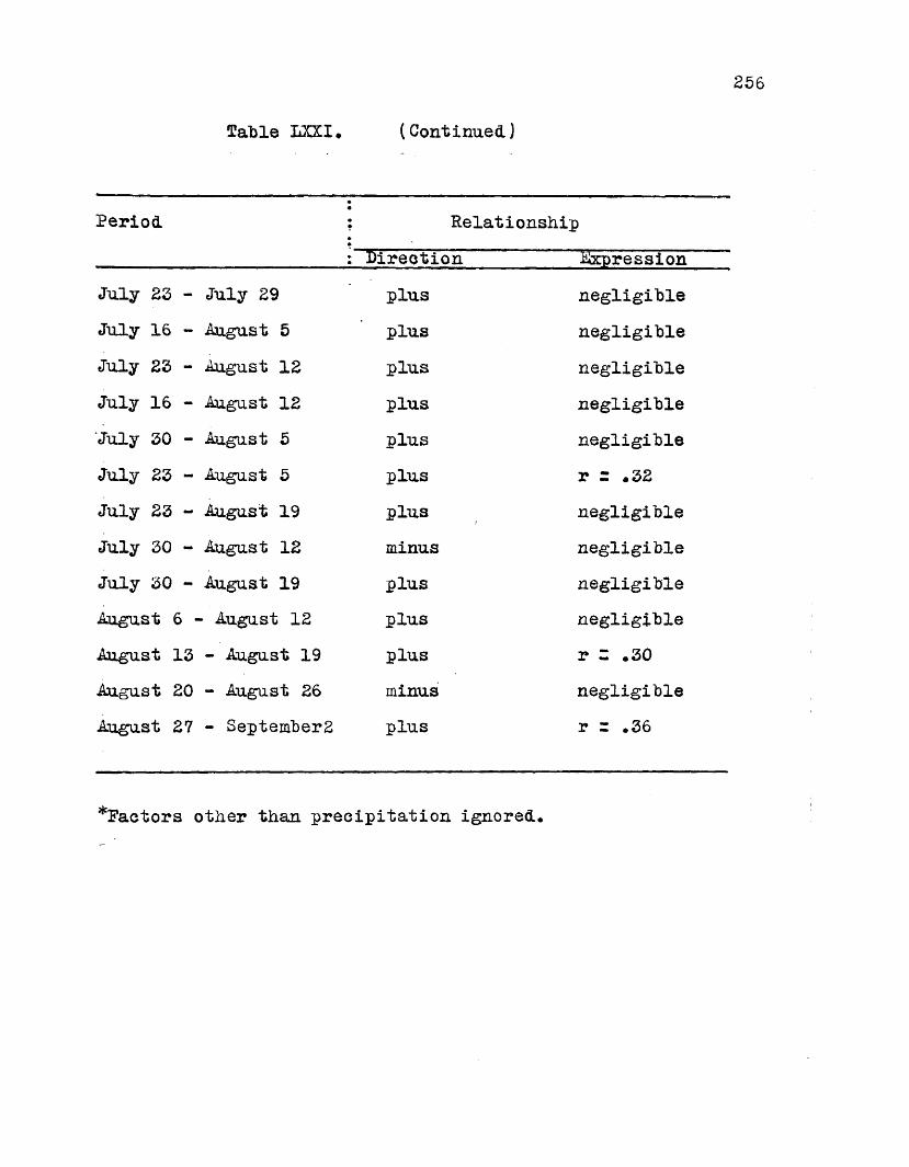
256

Table IiXXI. (Continued)

•*

Period : RelationshipDirection ■Expression

July 23 - July 29 plus negligibleJuly 16 - August 5 plus negligibleJuly 23 - August 12 plus negligibleJuly 16 - August 12 plus negligibleJuly 30 - August 5 plus negligibleJuly 23 - August 5 plus r = .32July 23 - August 19 plus negligibleJuly 30 - August 12 minus negligibleJuly 30 - August 19 plus negligibleAugust 6 - August 12 plus negligibleAugust 13 - August 19 plus r z .30August 20 - August 26 minus negligibleAugust 27 - September2 plus r z .36

*3?aetors other than precipitation ignored.

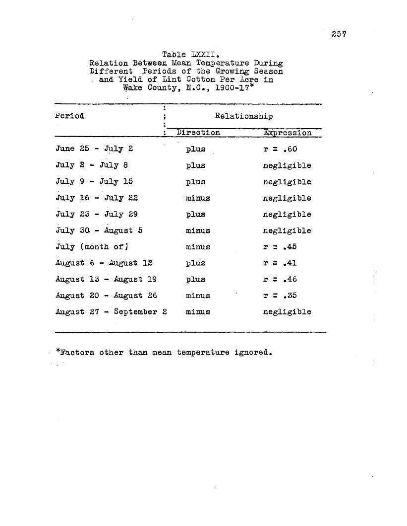
257

Table LXXII.Relation Between Mean Temperature During Different Periods of the Growing Season

and Yield of Lint Cotton Per Acre in fake County, R.C., 1900-17*

Period ; RelationshipDirection Expression

June 25 - July 2 plus oto«Itto

July 2 - July 8 plus negligibleJuly 9 - July 15 plus negligibleJuly 16 - July 22 minus negligibleJuly 23 - July 29 plus negligibleJuly 30. - August 5 minus negligibleJuly (month of) minus r = .45August 6 - August 12 plus ii • HAugust 13 - August 19 plus r = .46August 20 - August 26 minus r r .35August 27 - September 2 minus negligible

*Factors other than mean temperature ignored.

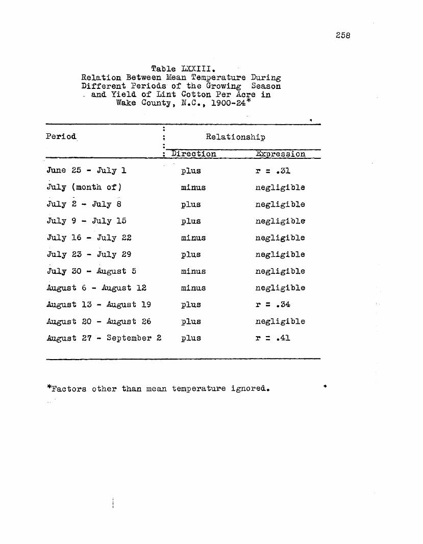
258

Table LXXIII.Relation Between Mean Temperature During Different Periods of the G-rowing Season - and Yield of Lint Cotton Per Acre in

Wake County, R.C., 1900-24*

Period RelationshipDirection depression

June 25 - July 1 plus r = .31July (month of) minus negligibleJuly 2 - July 8 plus negligibleJuly 9 - July 15 plus negligibleJuly 16 - July 22 minus negligibleJuly 23 - July 29 plus negligibleJuly 30 - August 5 minus negligibleAugust 6 - August 12 minus negligibleAugust 13 - August 19 plus r s .34August 20 - August 26 plus negligibleAugust 27 - September 2 plus HI.IIU

*Pactors other than mean temperature ignored*

259

Table LXXIV.Relation Between Minimum Temperature During

Different Periods of the G-rowing Season and Yield of Lint Cotton Per Acre in

Wake County, H.C., 1900-17*

••Period :

•

RelationshipDirection ^Expression

June 25 - J u l y 1 plus r = .52July 2 - July 8 minus negligibleJuly 9 - July 15 minus negligibleJuly 16 - July 22 minus negligibleJuly 23 - July 29 minus negligibleJuly 30 - August 5 minus negligibleAugust 6 - August 12 plus .ii

August 13 - August 19 plus negligibleAugust 19 - August 26 minus negligibleAugust 27 - September 2 plus negligible

*Faetors other than minimum temperature ignored

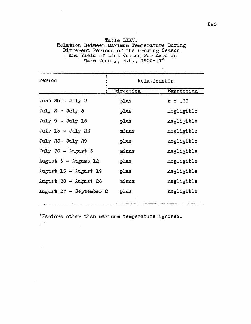
260

Table LOT.Relation Between. Iflaxinium Temperature Luring

Lifferent Periods of the Growing Season . sind Yield of Lint Cotton Per Acre in

Wake County, B.C., 1900-17*

Period ;•

Relationship• Lirection ^Expression

June 25 - July 2 plus 00to.Itu

July 2 - July 8 plus negligibleJuly 9 - July 15 plus negligibleJuly 16 - July 22 minus negligibleJuly 23- July 29 plus negligibleJuly 30 - August 5 minus negligibleAugust 6 - August 12 plus negligibleAugust 13 - August 19 plus negligibleAugust 20 - August 26 minus negligibleAugust 27 - September 2 plus negligible

*Faetors other than maximum temperature ignored.

261

Table LXXVT*Relation Between Maximum Temperature During

Different Periods of the Growing Season - and Yield of Lint Cotton Per Acre in

Wake County, M*C., 1900-24*

Period : RelationshipDirection Expression

June 25 - July 1 plus (—( •nu

July 2 - July 8 plus negligibleJuly 9 - July 15 plus negligibleJuly 16 - July 22 minus negligibleJuly 23 - July 29 minus negligibleJuly 30 - August 5 minus r = *30August 6 - August 12 minus negligibleAugust 13 - August 19 plus negligibleAugust 20 - August 26 minus negligibleAugust 27 - September 2 minus r z *33

*Pactors other than maximum temperature ignored*

262Weather Factors and Yield of Cotton in . Cumberland County, Horth Carolina*

While there are high degrees of relationship between single weather factors and yield of cotton, it would ordinarily seem likely that the combined effect of a number of them affords a more satisfactory basis for calculating the causal association between weather and yield* One of the reasons for this pre­sumption is because of the compensating tendencies among varia­tions in climatic conditions* The shedding of squares caused by excessive rainfall may be compensated by conditions which tend to reduce excessive vegetative growth, thus tending to favor the production of lint, while the effects of insufficient rainfall during the period of formation of bolls may be offset by high temperature and rainfall later in the season. It is difficult, of course, to procure a measure of all weather factors which can be incorporated in a rigid mathematical equation for predictive purposes. Some climatic conditions do not lend themselves to numerical measurement, and these are often the ones which offset the favorable and unfavorable effects of those which can be accurately measured. This accounts for many of the short«*time reversals in yield response, and it implies the practicability of production estimates on the basis of con­dition pars*

Table LXXVII shows the measures of alienation between actual yields of cotton in Cumberland County and the yields as

263

estimated, from the combined effects of various weather factors at clifferent periods of the growing season, fhe estimates of least-square straight line residuals of yield per acre are made by multiplying the relative weights of various weather factors as shown in tables LXIV and HX.Y by the least-square line resid­uals of the corresponding weather factor and then summating* fhe total algebraic sum of the products thus obtained is the estimated straight line residuals of yield per acre. As a measure of alienation between actual and estimated yields the standard error of estimated residuals is divided by the standard deviation of the actual residuals to obtain the numerical ex­pression which shows the relative magnitude of the extent to which the actual and estimated yield residuals deviate from their respective bases* In the case of the standard deviation the mean of the straight line residuals is taken as the base from which deviations are measured, while the standard error is based on the deviations of actual residuals from estimated residuals. The extent to which the standard error approaches the size of the standard deviation is an indication of the degree of alienation between actual and estimated yields, while the extent to which it tends to a minimum is indicative of a greater degree of approach to absolute accuracy in estimates*

264

Table IX20/TI.The Standard. Error of Estimate of Least-Square

Residuals of Yield and the Measure of Alienation Between Actual and Estimated Residuals of Yield

of Cotton Per Acre in Cumberland County, Eorth Carolina, 1904-24*

FactorsCorrelated

Standard Deviation of Actual Residuals

Standard Error of Estimated Residuals

Measureof

Alienation

Six weather factors and yield. (ABCEFQ.X) 57.60 47.50 .82

Twenty weather factors and yield.(ABCDEFG-HIJKLM EOPQRST.X) 57.60 55.30 .96

*Based on data in Tables LXIII, LXIV, and 1XV. The estimates of residuals of yield per acre are made by multiplying the residuals of the weather factors by their respective weights and then summating. The product thus obtained is the esti­mated residual of the line of least-squares representing the trend of cotton yields per acre. The standard error is calcu­lated by extracting the root-mean-square of the deviations of the actual residuals of the least-square line of yield from the estimated residuals of the least-square line of yield. The measure of alienation is calculated by dividing the standard error by the standard deviation.

265Planting Pates

Cotton planting begins usually from the middle to the last of March in extreme southern Texas and northern Florida, about April first in the Black Waxy Prairie of Texas, in central Louisiana, central Alabama, and central Georgia, and about April twenty-first along the northern margin of the Cotton Belt, Plant ing is general during the month of April, and it usually ends by May twenty-first Table LXXVIII shows the mean dates whenplanting begins, becomes general, and ends in the important cotton-producing States, On an average the plantings of eight States, Texas, Georgia, Alabama, Oklahoma, Mississippi, Arkansas, South Carolina, and Uorth Carolina comprise about 95 per cent, of the total cotton acreage of the entire Country^). The har­vested production of these eight States constitutes approximately 91 per cent, of the total ginnings of all States Thesefacts are of great potential assistance to the reporters of the United States Department of Agriculture, or any other agency engaged in making forecasts of the current yearls crop. When the acreage of the various States is known, together with the percentage of the total ginnings the acreage ordinarily repre­sents, there is possibility of still further perfecting the forecasts of production on the basis of condition pars,(1) Reported by Miss Rina Anderson, Bureau of Agricultural

Economics, United States Department of Agriculture,(2) Based on total acreage for the years 1912-26, inclusive,(3) Based on total production of lint cotton for the years

1912-26, inclusive.

266Table ixxrai.

Mean Dates When Planting of Cotton Begins, - Becomes General, and Ends*

State Planting Time: Beginning . General Ending

Texas March 29 April 13 May 9Oklahoma April 18 May 2 May 24Mississippi April 5 April 21 May 11Arkansas April 15 April 28 May 13Alabama April 8 April 20 May 11Georgia April 5 April 21 May 12Horth Carolina April 19 May 1 May 16South Carolina April 5 April 22 May 12Louisiana March 29 April 21 May 7Tennessee April 21 May 2 May 16Missouri April 25 May 4 May 14Florida March 16 March 28 April 20

*Yearbook of the U.S.D.A., 1922, page 989, Table 530. The States are arranged in descending order of total production for 1926. Planting dates for California, Arizona, Hew Mexico, and Virginia, which in volume of total production for 1926 follow Missouri in the order named, are not reported. The early ascertainment of acreage planted, i/hich differs but slightly from acreage ultimately harvested, is indespensable in estimating current production by the par method.

267

Monthly Harvestings

In knowing from month to month the percentage of the total cotton crop that is ordinarily harvested by a certain date the cotton trade is enabled to estimate to a fairly accurate degree the size of the current yearTs crop before the final ginnings report is issued by the Government. This is of particular interest to those who have cotton to sell as well as those who are buying, since they are in a position to predict the most probable trend of prices in the ensuing months, Table LXXIX shows the percentage of the crop that is harvested, on an average, during each month of the year. At the end of September about 45 per cent, of the crop has been harvested,79 per cent, at the end of October, and approximately 95 per cent* at the end of November. There are conditions, of course, which tend to modify these percentages, but it is not likely that changes from normal are often so marked throughout the United States as to alter greatly the averages given. Hence, if at the end of October 10,000,000 bales have been harvested, it is fairly safe to conclude that this number represents 79 per cent, of the total production, and if the harvestings at the end of Hovember total 12,000,000 bales it will not be far from accurate to state that this figure is equal to about 95 per cent, of the year’s crop. The early ascertainment of actual harvestings and ginnings is important to the cotton trade, and when the size of the crop is fairly accurately known the trend of subsequent monthly prices and the next year’s acreage can be predicted to a considerable degree.

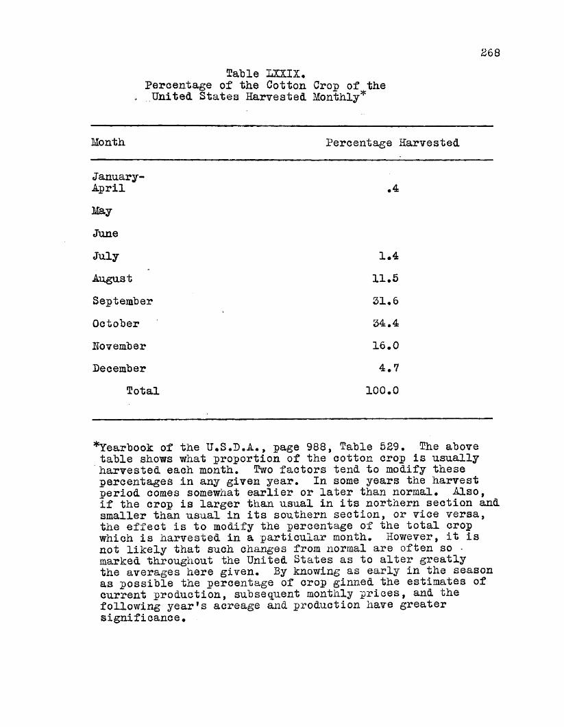
268Table LXXIX#

Percentage of the Cotton Crop of the, United States Harvested Monthly*

Month Percentage Harvested

January-April #4MayJuneJuly 1.4August 11.5September 31.6October 34.4November 16.0December 4.7

Total 100.0

*Yearbook of the U.S.D.A., page 988, Table 529* The above table shows what proportion of the cotton crop is usually harvested each month. Two factors tend to modify these percentages in any given year. In some years the harvest period comes somewhat earlier or later than normal# Also, if the crop is larger than usual in its northern section and smaller than usual in its southern section, or vice versa, the effect is to modify the percentage of the total crop which is harvested in a particular month. However, it is not likely that such changes from normal are often so - marked throughout the United States as to alter greatly the averages here given. By knowing as early in the season as possible the percentage of crop ginned the estimates of current production, subsequent monthly prices, and the following yearfs acreage and production have greater significance#

Ratio Estimates of Total Production269

The yield of cotton per acre most likely to occur in any year is the normal, the average for a period of years preceding any specified year. By calculating a moving average from year to year for a period of sufficient length to allow abnormal trends to be smoothed out it is possible to determine the most probable yield per acre of the current or following year* In Table LXXX are the calculated yield and acre ratios for the years 1900-27, inclusive, and the actual and estimated total production. The yield ratio is obtained by dividing the nine-year average of yield ending with the year preceding the specified year by the yield of the preceding year. This gives the most probable yield ratio for the current year. The acreage ratio is the product obtained by dividing the current yearTs acreage by the acreage of the preceding year. The product of the yield and acreage ratios and the total production of the preceding year represents the most probable production of the current year. As will be seen in Table LXXX the actual and estimated production tend to be equal. The greatest discrepancies occur in 1921 and 1922, when the yields per acre were abnormally low. In spite of this, however, the total estimated production of 353,723,000 bales for the entire twenty-eight year period was only 3.3 per cent, greater that the total actual production of 342,238,000 bales.The yearly average difference between estimated and actual pro­duction was only 410,000 bales. For the twenty-one year period,

2701900-20, inclusive, the degree of approach to accuracy is even greater than that for the period of twenty-eight years. The total estimated production for this period was 261,799,000 hales, as compared with a total actual production of 253,898,000 bales.This means that the estimated production for the entire period was only 3.1 per cent, greater than the actual production, con­stituting a yearly average difference of 376,000 bales between estimated and actual*

The degree of approach to absolute accuracy of production estimated by this method is of considerable significance because the estimate for the current year is made as soon as the extent of plantings is known* Therefore, the indications are that as soon as the Department of Agriculture issues its report on acreage in the Spring it is possible to predict, on an average, within less than a half million bales the current year’s production* This prediction assumes even greater significance when one realizes that it is made before the growing season scarcely begins.

In connection with estimates of production it is interesting to recall the percentage changes in acreage as estimated on the basis of relationship between deflated December spot prices and subsequent acreage of cotton harvested. Table LX shows that over a period of years the averages of percentage changes in actual and estimated acreage are identical. This indicates that on the basis of relationship between December prices and subse­quent acreage the most probable production of the following year

271

can be fairly accurately determined before any of the cotton is planted, since over a period of years the estimated acreage is approximately the same as the actual acreage. Hence, the production for the crop year following current quotations for December tends to be equal to the sum obtained by multiplying the product of the acreage and production ratios as calculated in lable LXXX by the acreage as estimated at the end of December. On an average this gives, one year in advance of the Government report on final ginnings, an estimate of the following yearTs crop that approaches in a very high degree the total actual production. ®ae Recapitulation following £able LXXXII shows the exact measurement of the degree of accuracy.

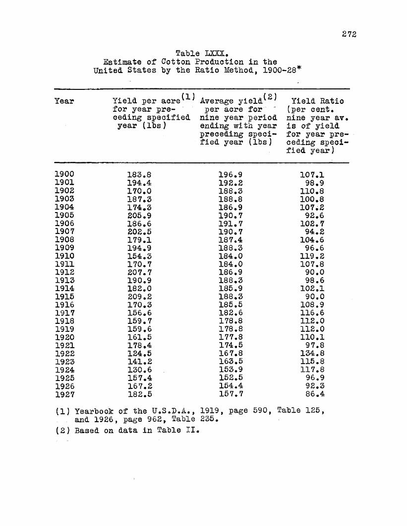
272

Table LXXS.Estimate of Cotton Production in the

United States by the Ratio Method, 1900-28*

Year (1)Yield per acre' ' for year pre­ceding specified year (lbs)

(2 )Average yield ' per acre for "

nine year period ending with year preceding speci­fied year (lbs)

Yield Ratio (per cent* nine year av. is of yield for year pre­ceding speci­fied year)

1900 183.8 196.9 107.11901 194.4 192.2 98.91902 170.0 188.3 110.81903 187.3 188.8 100.81904 174.3 186.9 107.21905 205.9 190.7 92.61906 186.6 191.7 102.71907 202.5 190.7 94.21908 179.1 187.4 104.61909 194.9 188.3 96.61910 154.3 184.0 119.21911 170.7 184.0 107.81912 207.7 186.9 90.01913 190.9 188.3 98.61914 182.0 185*9 102.11915 209.2 188.3 90.01916 170.3 185.5 108.91917 156.6 182.6 116.61918 159.7 178.8 112.01919 159.6 178.8 112.01920 161.5 177.8 110.11921 178.4 174.5 97.81922 124.5 167.8 134.81923 141.2 163.5 115.81924 130.6 153.9 117.81925 157.4 152.5 96.91926 167.2 154.4 92.31927 182.5 157.7 86.4(1) Yearbook of the U.S.D.A., 1919, page 590, Table 125,

and 1926, page 962, Table 235.(2) Based on data in Table II.

Table LXXX. (Continued)

273

(3) (3)Production of, .Actual pro- , Estimated pro- preceding Auction in Auction inyear in thou- thousands thousandssands of bales of bales of bales

for current (production ofyear preceding year

times the product of the yield and acre ratios)

102.5 9,345 10,123 10,257107.4 10,123 9,510 10,752101.5 9,510 10,631 10,69699.5 10,631 9,851 10,661

115.4 9,851 13,438 12,18786.8 13,438 10,575 10,800

115.7 10,575 13,274 12,56694.5 13,274 11,107 11,816

109.4 11,107 13,242 12,71095.4 13,242 10,005 12,202

104.7 10,005 11,609 12,486111.2 11,609 15,693 13,91695.1 15,693 13,703 13,431

108.2 13,703 14,156 14,61899.3 14,156 16,135 14,35285.3 16,135 11,192 12,386

111.4 11,192 11,450 13,57696.7 11,450 11,302 12,909

106.4 11,302 12,041 13,46893.2 12,041 11,421 12,568

106.9 11,421 13,440 13,44285.0 13,440 7,954 11,172

108.3 7,954 9,755 11,611112.4 9,755 10,140 12,696111.4 10,140 13,628 13,307111.3 13,628 16,104 14,698102.2 16,104 17,977 15,19185.3 17,977 12,782 13,249(3) Yearbook of the U.S.D.A*, 1919, page 590, Table 125, . , and 1926, page 962, Table 235.

Acreage ratio (per cent, current year’s acreage is of preceding year)

Table hXXX. (Continued)

*The total actual production in thousands of bales for the twenty-eight years was 342,£38* The total estimated production in thousands of bales for the same period was 353,723* The estimated production exceeded the actual production by 11,485,000 bales, constituting an average of 410,000 bales per year. For the entire period the estimated production ex­ceeded the actual production by 3.3 per cent. As will be observed in Table II, the per acre yields in 1921,- 1922, and 1923 were abnormally low. In spite of this, however, the error involved in the estimates is almost negligible. For the period 1900-20, inclusive, the error involved in the esti­mates is even more negligible, as the following figures will show. The total actual production for the twenty-one year period, expressed in thousands of bales, was 253,898. The total estimated pro­duction in thousands of bales for the same period was 261,799. The estimated production exceeded the actual production by 7,901,000 bales, which was an average of 376,000 bales per year. For the entire twenty-one year period the estimated pro­duction exceeded the actual production by 3.1 per cent.

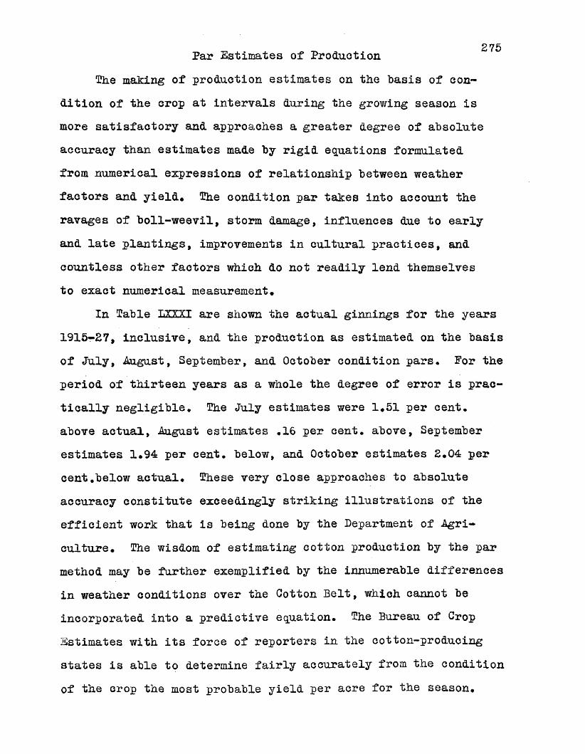
Par Estimates of Production Che making of production estimates on the basis of con­

dition of the crop at intervals during the growing season is more satisfactory and approaches a greater degree of absolute accuracy than estimates made by rigid equations formulated from numerical expressions of relationship between weather factors and yield* Che condition par takes into account the ravages of boll-weevil, storm damage, influences due to early and late plantings, improvements in cultural practices, and countless other factors which do not readily lend themselves to exact numerical measurement*

In Cable UQQCI are shown the actual ginnings for the years 1915-27, inclusive, and the production as estimated on the basis of July, August, September, and October condition pars. For the period of thirteen years as a whole the degree of error is prac­tically negligible* Che July estimates were 1*51 per cent, above actual, August estimates .16 per cent, above, September estimates 1*94 per cent, below, and October estimates 2*04 per cent.below actual. Chese very close approaches to absolute accuracy constitute exceedingly striking illustrations of the efficient work that is being done by the Department of Agri­culture* The wisdom of estimating cotton production by the par method may be further exemplified by the innumerable differences in weather conditions over the Cotton Belt, which cannot be incorporated into a predictive equation. Che Bureau of Crop Estimates with its force of reporters in the cotton-producing states is able to determine fairly accurately from the condition of the crop the most probable yield per acre for the season.

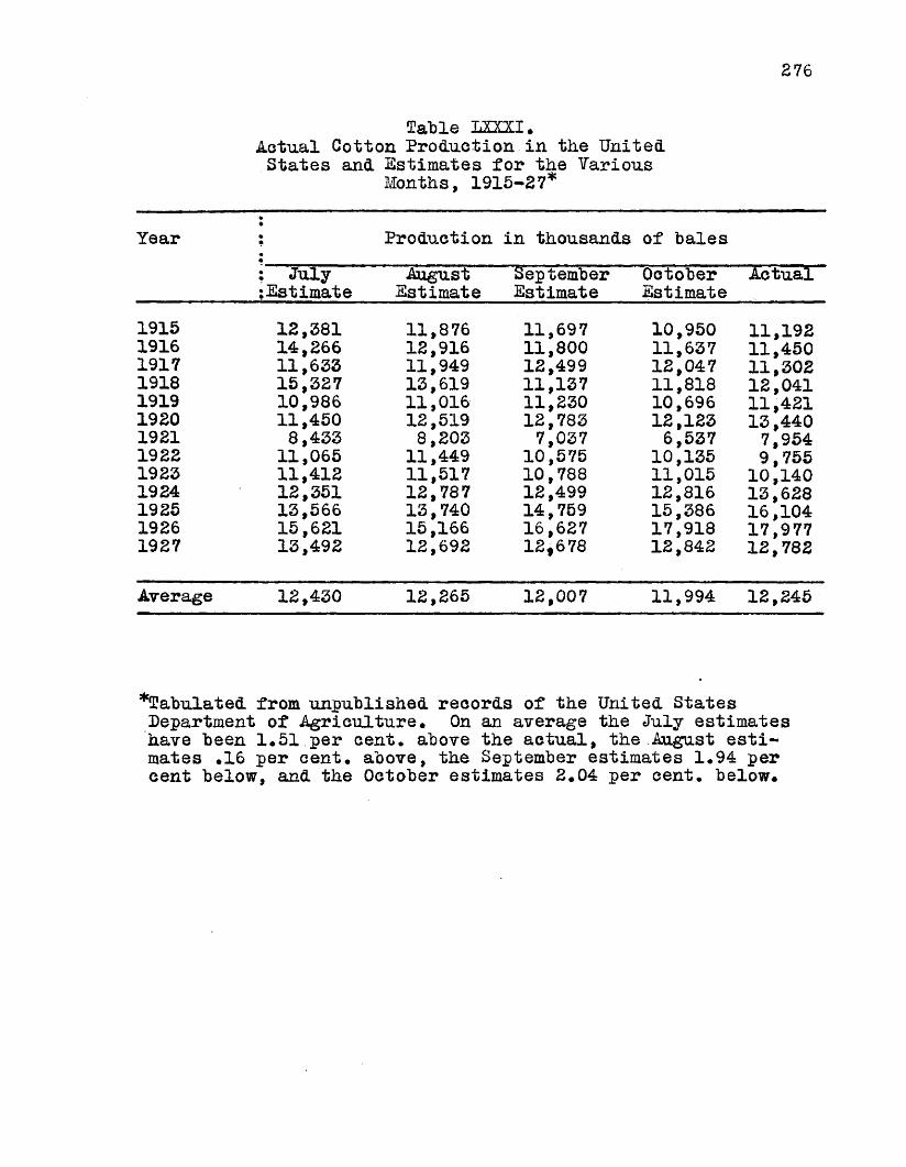
276

Cable LXXXI.Actual Cotton Production in the United States and Estimates for the Various

Months, 1915-27*

Year•*

•••

Production in thousands of bales: July : Estimate

AugustEstimate

SeptemberEstimate

OctoberEstimate

Actual

1915 12,381 11,876 11,697 10,950 11,1921916 14,266 12,916 11,800 11,637 11,4501917 11,633 11,949 12,499 12,047 11,3021918 15,327 13,619 11,137 11,818 12,0411919 10,986 11,016 11,230 10,696 11,4211920 11,450 12,519 12,783 12,123 13,4401921 8,433 8,203 7,037 6,537 7,9541922 11,065 11,449 10,575 10,135 9,7551923 11,412 11,517 10,788 11,015 10,1401924 12,351 12,787 12,499 12,816 13,6281925 13,566 13,740 14,759 15,386 16,1041926 15,621 15,166 16,627 17,918 17,9771927 13,492 12,692 12f678 12,842 12,782

Average 12,430 12,265 12,007 11,994 12,245

^Tabulated from unpublished records of the United States Department of Agriculture. On an average the July estimates have been 1.51 per cent, above the actual, the August esti­mates .16 per cent, above, the September estimates 1.94 per cent below, and the October estimates 2.04 per cent, below.

277

Relation Between Actual and Estimated Production

To further illustrate the degree of accuracy of par esti­mates of production numerical expressions were calculated to show the relationship between estimated and actual ginnings.The footnote to Table LXXXII shows these relationships in terms of coefficients of correlation calculated by the sum-product method. These high degrees of associated relationships con­sidered in connection with estimated and actual production as shown in Table LXXXI point to the rather definite conclusion that the present forecasting methods as employed by the United States Department of Agriculture are to be commended quite highly for their degree of approach to absolute accuracy.

Charts XXX to XXXIII, inclusive, show graphically the relation between actual production of cotton and the production as estimated on the basis of July, August, September, and October condition pars. The data are plotted in terms of multi­ples of standard deviation, and the two series are, therefore, directly comparable It will be observed that estimatedproduction tends in a very high degree to be the same as the actual production*

(1) The multiples of standard deviation are calculated from . the deviations of percentage changes from the mean of percentage changes of first differences.

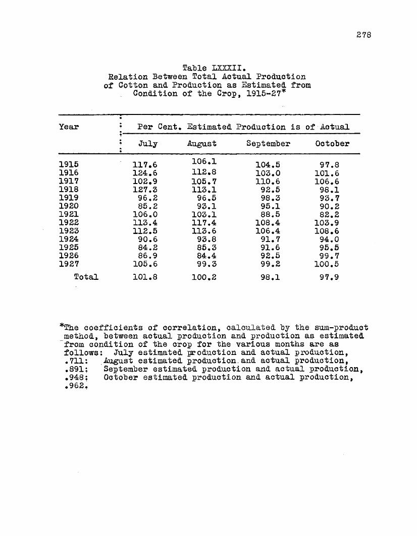
278

Table m i l ,Relation Between Total Actual Production of Cotton and Production as Estimated from

Condition of the Crop, 1915-27*

Year * Per Cent. Estimated Production is of Actual• " I — mmm t i wmw. .

? July August September October

1915 117.6 106.1 104.5 97.81916 124.6 112.8 103.0 101.61917 102.9 105.7 110.6 106.61918 127.3 113.1 92.5 98.11919 96.2 96.5 98.3 93.71920 85.2 93.1 95.1 90.21921 106.0 103.1 88.5 82.21922 113.4 117.4 108.4 103.91923 112.5 113.6 106.4 108.61924 90.6 93.8 91.7 94.01925 84.2 85.3 91.6 95.51926 86.9 84.4 92.5 99.71927 105.6 99.3 99.2 100.5

Total 101.8 100.2 98.1 97.9

*The coefficients of correlation, calculated by the sum-product method, between actual production and production as estimated from condition of the crop for the various months are as follows: July estimated production and actual production,• 711: .August estimated production, and actual production,.891: September estimated production and actual production,.948: October estimated production and actual production,.962.

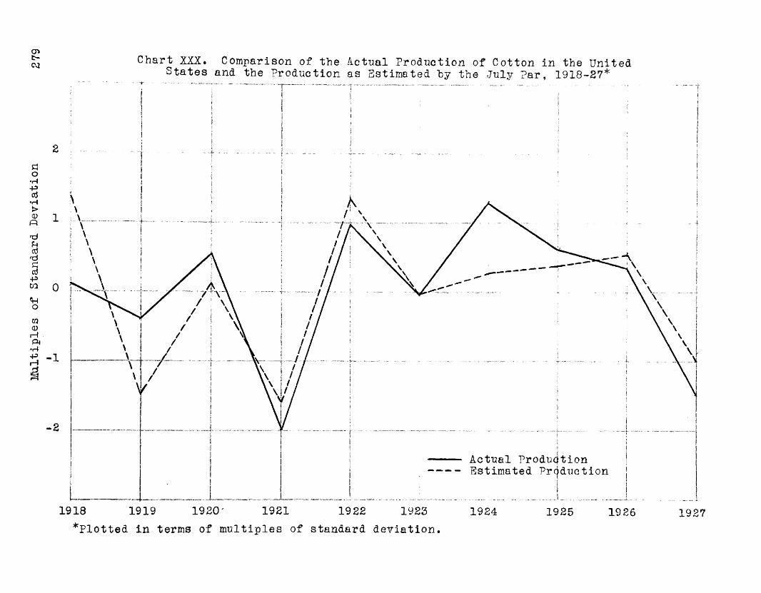
Multiples

of Standard

Deviation

279

Chart XXX. Comparison of the Actual Production of Cotton in the UnitedStates and the Production as Estimated by the July Par, 1918-27*

2

1

07 ' : T

\\

2

Actual Production Estimated Production

1918 1920' 19211919 1922 1923 1924 1925 1926 1927^Plotted in terms of multiples of standard deviation.

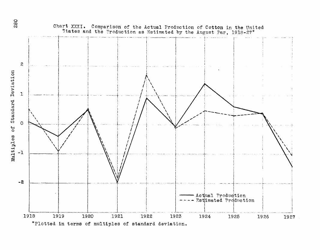
Multiples

of Standard

Devi

atio

no00 Chart XXXI# Comparison of the Actual Production of Cotton in the United

States and the Production as Estimated by the August Par, 1918-27*

2

1

0

1

s

Actjual Production Estimated Prcjduction

1918 1919 1920 1921 19231922 1924 1925 1926 1927'Plotted in terms of multiples of standard deviation#

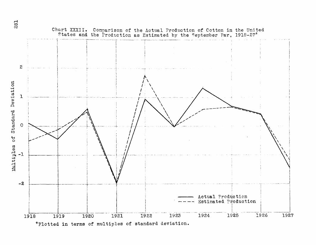
Multiples

of Standard

Devi

atio

ni—iCOC\2 Chart XXXII* Comparison of the Actual Production of Cotton in the United

States and the Production as Estimated by the September Par, 1918-27*

2

1

0

Actual Production Estimated Production

_J__1921 1925 1926 1927192419201919^Plotted in terms of multiples of standard deviation.

1918

Multiples

of Standard

Devi

atio

n

co Chart XX3CIII. Comparison of the Actual Production of Cotton in the UnitedStates and the Production as Estimated by the October Par, 1918-27*

2

1

0

1

2

Actual Production Estimated Production

19 27192619 2519241923deviation.

19 221919 1920 1921Plotted in terms of multiples of standard deviation

1918* standard

283

Recapitulation

As shown in Tables LX and LXI, it is possible to estimate with a considerable degree of approach to accuracy, several months prior to planting time, the acreage of cotton that is most likely to be harvested in the subsequent crop year. These estimates are based on the relationship between average December deflated spot quotations for Middling cotton at Dew York and Dew Orleans and the acreage of cotton actually harvested by farmers in the follow­ing crop year, affording a fairly accurate estimate of the size of the ensuing acreage several months before the planting season begins. Carrying the analysis further, it is possible to obtain at the end of December an estimate of the final ginnings one year in advance, before any of the cotton crop is planted and before the Government issues any report on acreage. By dividing the acreages as estimated in Table LXI by the acreage actually har­vested in the preceding year a product is obtained which expresses the ratio of estimated acreage for any subsequent crop year tothe acreage of the preceding year. The product of the acreage

f 1)ratio and the yield ratio as calculated in Table LXXX , multi­plied by the harvested acreage of the preceding crop year is the estimated production of the following year, and the production most likely to be reported in the Governments final estimate of ginnings one year later. The total actual production for the

(1) The yield ratio is calculated by computing the percentage that the average yield of the nine year period, ending with the year preceding the year for which estimates are to be made, is of the average yield for the preceding crop year.

284

years 1908-24, inclusive, was 206,266 thousands of hales, and the production as estimated at the end of December was 222,557 thousands of bales. The yearly average difference between estimated and actual production was 923,000 bales, meaning that for each ensuing year the crop as estimated on the basis of December spot prices was, on the average, 923,000 bales greater than the actual. For the years 1900-20, inclusive, the estimated production exceeded the actual by a yearly average of 632,000 bales, and for the two year period, 1923-24, the estimated production was 648,000 bales greater than the average of actual production. The high degree of approach to absolute accuracy in production estimates assumes greater significance when it is realized that they are made several months before the planting season begins in the South, and approximately one year in advance of the report on final ginnings as issued by the United States Department of Agriculture. On this basis, the cotton trade is enabled, one year in advance, to make a fairly accurate estimate of the total production of cotton that is most likely to result from the acreage as estimated at the - end of December.

285

II.

III.

17.

7.

71.

Conclusions.

There is, normally, a high degree of inverse relationship between current production of cotton in the United States and subsequent monthly prices of lint at American markets.

The relationship between domestic production of cotton and prices at American markets is greater than the relationship between domestic production and prices of American cotton at Liverpool.

The relationship between world production of cotton and prices in the United States and at Liverpool is no greater than the relationship between domestic production and domestic prices.

There is inverse correlation between exports and prices, and the multiple relationship between carry-over, current pro­duction, and exports is not appreciably greater than the simple correlation between domestic production and prices.

The relationship between consumption of cotton in the United States and prices of lint at imerican markets is inverse, indicating that prices are determined primarily by pro­duction, rather than by consumption.

Price predictions can be fairly accurately made on the basis of relationship between production and undeflated spot prices.

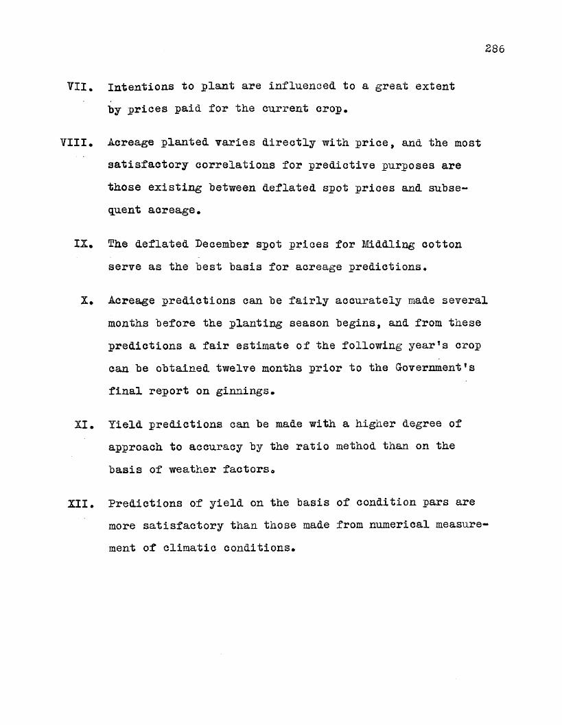
286

VII.

VIII.

IX.

X.

XI.

XII.

Intentions to plant are influenced to a great extent by prices paid for the current crop.

Acreage planted varies directly with price, and the most satisfactory correlations for predictive purposes are those existing between deflated spot prices and subse­quent acreage.

The deflated December spot prices for Middling cotton serve as the best basis for acreage predictions.

Acreage predictions can be fairly accurately made several months before the planting season begins, and from these predictions a fair estimate of the following year’s crop can be obtained twelve months prior to the Government1 s final report on ginnings.

Yield predictions can be made with a higher degree of approach to accuracy by the ratio method than on the basis of weather factors.

Predictions of yield on the basis of condition pars are more satisfactory than those made from numerical measure­ment of climatic conditions.

287

Literature Cited

(1) Moore, H.L. Forecasting the Yield and the Price - ~ of Cotton.

(2) Smith, B.B. Forecasting the Acreage of Cotton.

(3) Smith, B.B. Relation Between Weather Conditions . . and Yield of Cotton in Louisiana.

(4) Smith, B.B. Factors Affecting the Price of Cotton.