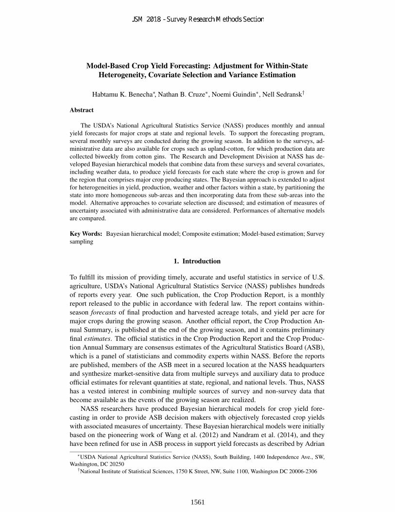
Model-Based Crop Yield Forecasting: Adjustment for Within-StateHeterogeneity, Covariate Selection and Variance Estimation

Habtamu K. Benecha∗, Nathan B. Cruze∗, Noemi Guindin∗, Nell Sedransk†

Abstract

The USDA’s National Agricultural Statistics Service (NASS) produces monthly and annualyield forecasts for major crops at state and regional levels. To support the forecasting program,several monthly surveys are conducted during the growing season. In addition to the surveys, ad-ministrative data are also available for crops such as upland-cotton, for which production data arecollected biweekly from cotton gins. The Research and Development Division at NASS has de-veloped Bayesian hierarchical models that combine data from these surveys and several covariates,including weather data, to produce yield forecasts for each state where the crop is grown and forthe region that comprises major crop producing states. The Bayesian approach is extended to adjustfor heterogeneities in yield, production, weather and other factors within a state, by partitioning thestate into more homogeneous sub-areas and then incorporating data from these sub-areas into themodel. Alternative approaches to covariate selection are discussed; and estimation of measures ofuncertainty associated with administrative data are considered. Performances of alternative modelsare compared.

Key Words: Bayesian hierarchical model; Composite estimation; Model-based estimation; Surveysampling

1. Introduction

To fulfill its mission of providing timely, accurate and useful statistics in service of U.S.agriculture, USDA’s National Agricultural Statistics Service (NASS) publishes hundredsof reports every year. One such publication, the Crop Production Report, is a monthlyreport released to the public in accordance with federal law. The report contains within-season forecasts of final production and harvested acreage totals, and yield per acre formajor crops during the growing season. Another official report, the Crop Production An-nual Summary, is published at the end of the growing season, and it contains preliminaryfinal estimates. The official statistics in the Crop Production Report and the Crop Produc-tion Annual Summary are consensus estimates of the Agricultural Statistics Board (ASB),which is a panel of statisticians and commodity experts within NASS. Before the reportsare published, members of the ASB meet in a secured location at the NASS headquartersand synthesize market-sensitive data from multiple surveys and auxiliary data to produceofficial estimates for relevant quantities at state, regional, and national levels. Thus, NASShas a vested interest in combining multiple sources of survey and non-survey data thatbecome available as the events of the growing season are realized.

NASS researchers have produced Bayesian hierarchical models for crop yield fore-casting in order to provide ASB decision makers with objectively forecasted crop yieldswith associated measures of uncertainty. These Bayesian hierarchical models were initiallybased on the pioneering work of Wang et al. (2012) and Nandram et al. (2014), and theyhave been refined for use in ASB process in support yield forecasts as described by Adrian

∗USDA National Agricultural Statistics Service (NASS), South Building, 1400 Independence Ave., SW,Washington, DC 20250

†National Institute of Statistical Sciences, 1750 K Street, NW, Suite 1100, Washington DC 20006-2306

1561

(2012) (for corn and soybeans), Cruze (2015, 2016) (winter wheat), and Cruze and Benecha(2017) (upland cotton). The yield forecasting models facilitate multiple outcomes:

• combination of current and historical predictions of yield obtained from multiplesurveys,

• incorporation of relavant auxiliary data and covariates such as weather informationand crop condition,

• and resulting consistent one-number yield forecasts and measures of uncertainty forregions and member states.

Because the current yield models for upland cotton and the other crops input data at stateand regional levels, any within-state heterogeneities in yield, production, and weather con-ditions may not be fully accounted for when forecasts are produced. For example, twodistinct clusters of upland cotton grown in Texas, the largest cotton producing state in theU.S., differ in terms of climate and typical annual cotton yield.

In this paper, we extend the existing upland cotton yield model of Cruze and Benecha(2017) by incorporating sub-state level data for Eastern and Western districts in Texas,with the intention of improving the state and regional yield forecasts and the correspondingstandard errors. The proposed model is compared with existing methods and its merits areassessed. Additionally, covariate selection and alternative approaches to characterizing thevariability for non-probability cotton ginnings data are also discussed. The paper is orga-nized as follows: In Section 2, the upland cotton speculative region and available sourcesof data for forecasting upland cotton yield in the context of the NASS publication timelineare described. In Section 3, yield estimates obtained from three distinct NASS surveys anda census of cotton processors (cotton gins) are compared. Estimates from two distinct clus-ters of cotton in Texas are compared. Section 4 describes a Bayesian hierarchical modelfor upland cotton. In Section 5, issues related to covariate selection and variances of yieldestimates from cotton ginnings are discussed. In section 6, a preliminary analysis assessingthe effects that result from assumptions about sub-state breakouts, choice of covariates, andassumptions of about uncertainty in cotton ginnings is presented. Concluding remarks aregiven in Section 7.

2. The speculative region, sources of data, and publication timelines

2.1 The upland cotton speculative region

Currently, NASS publishes estimates and forecasts of upland cotton yield, production, har-vested acreage and related statistics every month from August through January for thenation and the 17 southern states shown in the map in Figure 1. The six states in the dark-shaded area constitute the current speculative region. Together they account for most of theupland cotton production in the nation. While the membership of the upland cotton specu-lative region has changed over the years, the six states (Arkansas, Georgia, Louisiana, Mis-sissippi, North Carolina, and Texas) have constituted the region since 2008. Currently, thescope of the model-based approach is aimed at producing benchmarked and reproduciblemonthly yield forecasts and associated measures of uncertainty for these six states and thespeculative region as a whole.

1562

Figure 1: USDA NASS Upland Cotton Estimation Program States and Speculative Region

2.2 Sources of data for yield forecasting and NASS publication timelines

Forecasting and estimation of upland cotton yield in the Crop Production Report and theCrop Production Annual Summary is supported by a biweekly census of cotton gins inall cotton producing states, and by three probability-based surveys: the Objective YieldSurvey (OYS), the Agricultural Yield Survey (AYS) and the December Quarterly Acreage,Production, and Stocks (APS) survey. Approximate data collection windows for each ofthese sources and the associated publication deadlines are depicted in Figure 2. The OYSis based on field measurements collected at sampled field plots. It is conducted monthlyfrom August through January. The OYS covers only the six states in the speculative region,and it gives rise to monthly point predictions of regional and state yield with associatedstandard errors. The AYS is a monthly farmer interview survey conducted from August toNovember. Like the OYS, the AYS provides point predictions of state and regional levelyield and standard error estimates. The third NASS survey, the December APS survey is afarmer interview survey conducted near the end of the growing season in December. TheAPS survey is conducted after much of the crop is harvested and involves larger samplesizes than the OYS and the AYS. As a result, the APS survey gives rise to more accurateestimates of yield and with lower sampling variation.

A fourth source of data for estimation of upland cotton statistics is derived from abiweekly census of cotton processing gins in cotton producing states. In this exhaustivecensus, cotton processors (note, not farmers) are requested to report:

1. the number of bales of cotton already processed in the season as of a specified refer-ence date, and

2. the number of bales of cotton expected to be processed during the time interval fromthe reference date to the end of the crop year.

Based on these records, total production is projected for states and the nation. Althoughsome states begin reporting ginnings data in earlier months, projected cotton ginnings pro-duction data are available for all producing states starting from October of each year. Asa result, the ASB starts considering ginnings data in support of October forecasts, andcontinues to consider such data every month until the Crop Production Annual Summaryreport is released in January. By law, NASS must publish its official upland cotton yield

1563

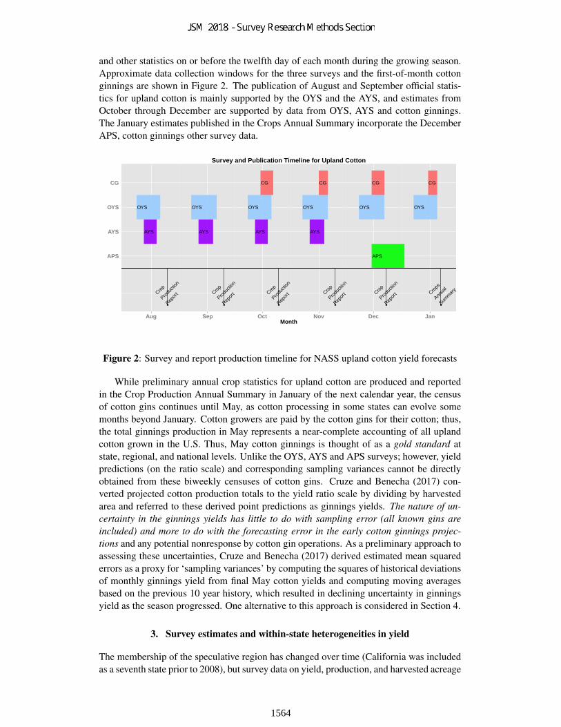
and other statistics on or before the twelfth day of each month during the growing season.Approximate data collection windows for the three surveys and the first-of-month cottonginnings are shown in Figure 2. The publication of August and September official statis-tics for upland cotton is mainly supported by the OYS and the AYS, and estimates fromOctober through December are supported by data from OYS, AYS and cotton ginnings.The January estimates published in the Crops Annual Summary incorporate the DecemberAPS, cotton ginnings other survey data.

APS

AYSAYSAYSAYS

OYSOYSOYSOYSOYSOYS

CGCGCGCG

● ● ● ● ● ●

Crop

Produ

ction

Repor

t Crop

Produ

ction

Repor

t Crop

Produ

ction

Repor

t Crop

Produ

ction

Repor

t Crop

Produ

ction

Repor

t Crops

Annua

l

Summ

ary

APS

AYS

OYS

CG

Aug Sep Oct Nov Dec JanMonth

Survey and Publication Timeline for Upland Cotton

Figure 2: Survey and report production timeline for NASS upland cotton yield forecasts

While preliminary annual crop statistics for upland cotton are produced and reportedin the Crop Production Annual Summary in January of the next calendar year, the censusof cotton gins continues until May, as cotton processing in some states can evolve somemonths beyond January. Cotton growers are paid by the cotton gins for their cotton; thus,the total ginnings production in May represents a near-complete accounting of all uplandcotton grown in the U.S. Thus, May cotton ginnings is thought of as a gold standard atstate, regional, and national levels. Unlike the OYS, AYS and APS surveys; however, yieldpredictions (on the ratio scale) and corresponding sampling variances cannot be directlyobtained from these biweekly censuses of cotton gins. Cruze and Benecha (2017) con-verted projected cotton production totals to the yield ratio scale by dividing by harvestedarea and referred to these derived point predictions as ginnings yields. The nature of un-certainty in the ginnings yields has little to do with sampling error (all known gins areincluded) and more to do with the forecasting error in the early cotton ginnings projec-tions and any potential nonresponse by cotton gin operations. As a preliminary approach toassessing these uncertainties, Cruze and Benecha (2017) derived estimated mean squarederrors as a proxy for ‘sampling variances’ by computing the squares of historical deviationsof monthly ginnings yield from final May cotton yields and computing moving averagesbased on the previous 10 year history, which resulted in declining uncertainty in ginningsyield as the season progressed. One alternative to this approach is considered in Section 4.

3. Survey estimates and within-state heterogeneities in yield

The membership of the speculative region has changed over time (California was includedas a seventh state prior to 2008), but survey data on yield, production, and harvested acreage

1564

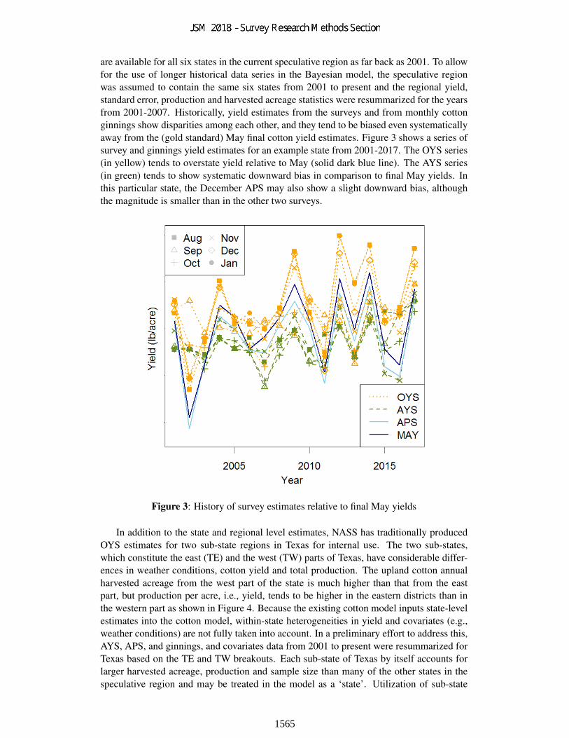
are available for all six states in the current speculative region as far back as 2001. To allowfor the use of longer historical data series in the Bayesian model, the speculative regionwas assumed to contain the same six states from 2001 to present and the regional yield,standard error, production and harvested acreage statistics were resummarized for the yearsfrom 2001-2007. Historically, yield estimates from the surveys and from monthly cottonginnings show disparities among each other, and they tend to be biased even systematicallyaway from the (gold standard) May final cotton yield estimates. Figure 3 shows a series ofsurvey and ginnings yield estimates for an example state from 2001-2017. The OYS series(in yellow) tends to overstate yield relative to May (solid dark blue line). The AYS series(in green) tends to show systematic downward bias in comparison to final May yields. Inthis particular state, the December APS may also show a slight downward bias, althoughthe magnitude is smaller than in the other two surveys.

Figure 3: History of survey estimates relative to final May yields

In addition to the state and regional level estimates, NASS has traditionally producedOYS estimates for two sub-state regions in Texas for internal use. The two sub-states,which constitute the east (TE) and the west (TW) parts of Texas, have considerable differ-ences in weather conditions, cotton yield and total production. The upland cotton annualharvested acreage from the west part of the state is much higher than that from the eastpart, but production per acre, i.e., yield, tends to be higher in the eastern districts than inthe western part as shown in Figure 4. Because the existing cotton model inputs state-levelestimates into the cotton model, within-state heterogeneities in yield and covariates (e.g.,weather conditions) are not fully taken into account. In a preliminary effort to address this,AYS, APS, and ginnings, and covariates data from 2001 to present were resummarized forTexas based on the TE and TW breakouts. Each sub-state of Texas by itself accounts forlarger harvested acreage, production and sample size than many of the other states in thespeculative region and may be treated in the model as a ‘state’. Utilization of sub-state

1565

level data in the model fitting processes may result in improved yield forecasts for the stateof Texas and for the speculative region as a whole. In addition to fitting models for thesix states, we investigate a scenario in which the two regions of Texas enter the models astwo separate states, the speculative region constitutes seven ‘states’ (i.e., AR, GA, LA, MS,NC, TE and TW) and the regional survey and cotton ginnings estimates are re-calculatedby excluding the state level TX data and by including estimates from TE, TW.

Figure 4: Annual yield estimates for two sub-states

4. Bayesian hierarchical model for yield forecasting

In this section, we outline extensions of the upland cotton yield model described in Cruzeand Benecha (2017). The extended model allows for the estimation of parameters at state,regional and sub-state levels for the two regions of Texas. Whereas Cruze and Benecha(2017) initially treated January ginnings yield as a ‘gold standard’ (in keeping with thepublication window), we introduce the May final yield as the gold standard and the quan-tity to be forecasted. For Texas in particular, where processing activity evolves beyondthe Annual Summary publication window, this decision represents a better choice of goldstandard.

4.1 Models for the speculative region

As discussed in Cruze and Benecha (2017), the Bayesian hierarchical models for the spec-ulative region and its member states specify conditional and marginal distributions for thedata and the parameters in three parts. The behavior of observed data given an underlyingprocess for yield is described in a data model and the parameter of interest (i.e., yield, de-noted by µt for the speculative region) is related to covariates of interest through a processmodel and prior distributions are specified for model parameters. Let yktm denote observed

1566

yield estimates from data source k ∈ {O,A,Q,G,M} for OYS, AYS, APS, ginnings yield(from October to January), and the May final yield respectively, in year t ∈ {1, 2, ..., T}and month m ∈ {8, 9, 10, 11, 12, 13}. Let s2ktm denote the variance of the yield estimatefrom source k in year t and month m. Assume for now that a variance estimate, s2Gtm, isavailable for ginnings yield. Conditional on the latent regional yield, µt, data models forforecast month m are described by

yktm|µt ∼ indep N(µt + bkm, s2ktm + σ2

km

), k = O,A, m ≤ 13 (1)

yQtm|µt ∼ indep N(µt + bQm, s2Qtm + σ2

Qm

),m = 13 (2)

yGtm|µt ∼ indep N(µt + bGm, s2Gtm + σ2

Gtm

),m = 10, 11, 12, 13 (3)

yM |µt ∼ indep N(µt, σ

2M

)(4)

In this specification, observed survey yields and ginnings yield estimates are modeled withpotential month-specific biases, whereas the May final yield estimates are used as a proxyfor the gold-standard May ginnings and assumed unbiased as shown in Equation 4. Al-though the last AYS survey of the season is conducted in November, estimates from theNovember survey may be included in the analyses for making the December and Januaryforecasts. Note also that estimates from the December Quarterly APS survey are used inthe January final model; data collection for the APS is onoing when December forecastsare due for publication. Given an appropriate sampling variance estimate, s2Gtm, the datamodel for yield from monthly ginnings takes the form shown in Equation 3. We considertwo scenarios, one in which an estimate of s2Gtm is obtained separately, and another inwhich we assume s2Gtm = 0.

The region-level process model varies around a mean based on a regression of historicend-of-season yield on observable covariates:

µt ∼ indep N(z′tβ, σ

2η

). (5)

Finally, the following prior distributions are specified for the parameters; bkm, β ∼ indepN(0, 106), σ2

km, σ2η , σ2

Gtm ∼ indep IG(.001, .001), and σ2M ∼ indep Uniform (.0005, .001).

The collection of data and process model parameters are denoted Θd ≡(bkm, σ2

km, γ2Gm, σ2M

)and Θp ≡

(β, σ2

η

), respectively.

Under the assumption of conditional independence, the likelihood function has the mul-tiplicative form

[yO, yA, yQ, yG|µt,Θd] =∏

k∈{O,A,Q,G}

[yk|µt,Θd] (6)

and by Bayes’ Rule, the posterior distribution of model parameters given observable yieldestimates is shown in Equation 7:

[µt,Θd,Θp|yO, yA, yQ, yG] ∝∏

k∈{O,A,Q,G}

[yk|µt,Θd][µ|Θp][Θd][Θp]. (7)

A Gibbs sampling algorithm is employed to obtain estimates of all model parameters.(See, e.g., Gelman et al. (2003).) For brevity, only the full conditional distribution forregional yield µt is shown:

[µt|yO, yA, yQ, yG|Θd,Θp] ∼ N

(∆2

∆1,1

∆1

)(8)

1567

where

∆1 =∑

k=O,A

1

σ2km + s2ktm

+Im∈{10,...,13}

σ2Gtm + s2Gtm

+I{m=13}

σ2Q,13 + s2Qt,13

+1

σ2η

(9)

∆2 =∑

k=O,A

yktm − bkmσ2km + s2ktm

+ Im∈{10,...,13}yGtm − bGm

σ2Gtm + s2Gtm

(10)

+I{m=13}(yQt,13 − bQ,13)

σ2Q,13 + s2Qt,13

+z′tβ

σ2η

.

Equation 9 describes the sum of the precisions of each information source. DividingEquation 10 by Equation 9, the mean of the full conditional distribution Equation 8 isshown to be a weighted average of available information sources: the bias-corrected AYSand OYS indications, the bias corrected quarterly APS indication (when it is available),bias corrected ginnings , and covariates information. Since NASS does not publish theindividual inputs, this relationship serves as a useful interpretation for the one number yieldforecast as a meaningful composite of the available information based on posterior variance;the most precise information sources receive a proportionally larger share of weight indetermining the overall yield forecast.

4.2 Models for states

We consider two alternative models for states: one for the six states in the current specula-tive region (i.e, AR, GA, LA, MS, NC and TX), and one in which the two sub-state regionsof Texas enter the model as separate ‘states’, i.e., AR, GA, LA, MS, NC, TE, and TW.and the regional survey, ginnings and covariate data are re-calculated based on the new setof member states. In the following discussions, the state index j takes values from 1 to 6when TX is included in the speculative region and takes values from 1 to 7 when TE andTW are included in the region as two distinct states. Data and process models for the statesresemble those of the speculative region with models for each state j given by:

yktmj |µt ∼ indep N(µtj + bkmj , s

2ktmj + σ2

kmj

), k = O,A, m ≤ 13 (11)

yQtmj |µt ∼ indep N(µtj + bQmj , s

2Qtmj + σ2

Qmj

),m = 13 (12)

yGtmj |µt ∼ indep N(µtj + bGmj , s

2Gtmj + σ2

Gtmj

),m = 10, 11, 12, 13 (13)

yMj |µt ∼ indep N(µtj , σ

2Mj

)(14)

Prior distributions are specified on the data and process model parameters of each stateas before. The full conditional distribution of yield in the jth state, µtj resembles Equa-tion 8. Assuming independence, the collection of state-level crop yields follows a multi-variate normal distribution.

[µt·|y,Θd,Θp] ∼ indep MV N

(vec

(∆2tj

∆1tj

), diag

(1

∆1tj

))(15)

While yield parameters for the region µt and states µtj must respect the balance identityµt =

∑j wjµtj , estimates of parameters µtj derived under Equation 15 may not. There-

fore, it is desirable to enforce the balance constraint between the speculative region andmember states. Iterates of the speculative region MCMC simulation are fed into the MCMCsimulation for a ‘constrained’ state level model. By conditioning the vector of state-level

1568

yields in Equation 15 on the restriction that their weighted sum is equal to forecasted spec-ulative region yield µt, the collection of the first j − 1 states will follow a multivariatenormal distribution (

µt1, µt2, . . . , µt(J−1)

)∼ MVN(µ, Σ). (16)

At each time t, the yield for the J th state is given by

µtJ = µt −1

wtJ

J−1∑j=1

wtjµtj , (17)

which resembles the top-down procedure used during the ASB’s own decision makingprocess. Posterior means obtained from the Monte Carlo samples under Equation 8, Equa-tion 16, and Equation 17 represent a collection of point estimates for the speculative regionand all its constituent states that honor the physical balance constraint. Standard errors ofthese estimates are derived as the square root of posterior variances, giving rise to defensi-ble measures of uncertainty at both spatial scales.

5. Covariates and variances for ginnings yield

5.1 Covariates and covariate selection

Estimates of the latent mean parameters (i.e., µt and µtj) in Sections 4.1 and 4.2 are relatedto a number of factors that affect upland cotton yield. The existing cotton model includesaverage precipitation (PCP), average cooling degree days (CDD), crop condition ratings(COND) and a drought sevierity index (DRT) as covariates to model µt and µtj . Thesecovariates were choosen based on a combination of exploratory analysis and expert sug-gestions. Using a similar approach, two more predictors are added to the pool of potentialcovariates for consideration in our analysis. The additional covariates are monthly maxi-mum temprature (TMP) and monthly killing degree days (KDD), resulting in a total of sixpotential covariates (i.e., PCP, CDD, COND, DRT, TMP and KDD) to choose from. Animportant task in selecting predictors from the pool is determining the week or month inwhich each covariate has the highest impact on yield. Determining a subset of the pool ofcovariates that gives an optimal fit to the model is another important consideration. Pre-liminary attempts were made to address these issues by applying formal covariate selectionprocedures. For example, spike-and-slab priors, as described in Ishwaran and Rao (2005),were applied to select the optimal covariate combination with the month in which eachselected covariate impacts yield the most. Stepwise regression and least absolute shrink-age and selection operator (LASSO) approaches were also applied to select covariates fora model that uses the May final yield as a response variable. Application of the variableselection procedures resulted in different sets of optimal covariates for different states. Inaddition, selected covariate sets vary by forecasting months in a season. At this time, weconsider a common set of covariates observed on each state to make yield forecasts.

The covariate selection process is still an ongoing research project. For comparisons,model-based forecasts were made using a modified version of the covariates in the existingmodel (i.e., {PCP, CDD, COND, DRT}) and by using a tentatively selected set of covariates{PCP, TMP, KDD, COND}. In year t, the distribution of the latent mean yield parameterfor state i can be expressed using the two covariate sets as

µtj ∼ N(βj1 + βj2PCPj + βj3CDDj + βj4CONDj + βj5DRTj , σ

2η

), and

µtj ∼ N(βj1 + βj2PCPj + βj3TMPj + βj4KDDj + βj5CONDj , σ

2η

).

Where,

1569

• CDDj is the number of cooling degree days (a proxy for cumulative growing degreedays) during July

• PCPj is the state’s average precipitation during the month of July

• CONDj : is the percent of the cotton crop that has been rated excellent as of week 28according to NASS’s crop condition ratings.

• DRTj is percent of land in the sate with extreme and exceptional drought in July

• KDDj is average July killing degree days

• TMPj Maximum temprature during July.

For the speculative region model, the corresponding covariate values are calculated asweighted sums of the state level covariates.

5.2 Variances for ginnings yield

Unlike the OYS, AYS and APS surveys, yield estimates from ginnings have no associateddesign-based variance estimates. As described in Sections 4.1 and 4.2, the model assumesthat the variances of the conditional distributions of yield estimates from OYS, AYS andAPS are sums of the corresponding sampling variances and a parameter characterizingvariation due to ‘other’ non-sampling sources as in

yGtmj |µt ∼ indep N(µtj + bGmj , s

2Gtmj + σ2

Gtmj

),m = 10, 11, 12, 13. (18)

To allow for a similar variance specification for ginnings yield estimates, Cruze and Benecha(2017) initially estimated variances for ginnings yield using deviations of the monthly gin-nings yield estimates from the May final yield. In some since, this approach may havepenalized ginnings data twice, since the biases in early season ginnings drove both thes2Gtmj and the term related to non-sampling errors. In this work, we consider two alterna-tive approaches:

• Assumption 1: s2Gtmj = 0,

• Assumption 2: s2Gtmj is an estimated quantity.

Under the second assumption, we estimate s2Gtmj based on a model for the May final yieldthat includes monthly ginnings yield and OYS yield as covariates.

6. Application to the 2015, 2016 and 2017 upland cotton yield

The model and the methods discussed in Section 4 were applied to revisit the 2015, 2016and 2017 upland cotton yield forecasts. Models were fitted for the current speculativeregion and its member states (i.e., AR, GA, LA, MS, NC, and TX). Another set of modelswere fitted for AR, GA, LA, MS, NC, TE and TW, and the speculative region, based onre-calculated survey, ginnings and covariate estimates. In the following discussions, werefer to the first model as the six-state model and the second model as the seven-statemodel. Each of the two models were fitted using two different sets of covariates (i.e., (PCP,CDD, COND, DRT) and (PCP, TMP, KDD, COND)) and under the two assumptions aboutthe variances for the conditional distributions of ginnings yield estimates from October toJanuary. In all, these represent 2×2×2 specifications. We describe select outcomes below.

1570

Figure 5: Published and model forecasts based on covariate set {PCP,CDD,DRT,COND}for 2016

Figure 6: Published and model forecasts based on covariate set {PCP,TMP,KDD,COND}for 2016

Figures 5 and 6 show the 2016 forecasts based on covariate sets (PCP, CDD, COND,DRT) and (PCP, TMP, KDD, COND) applied to the seven state model with Assumption 2for the variance of the conditional distribution of ginnings yield. States A, B, C, D, E and Frepresent the six member states of the speculative region, where the model-based forecastsfor Texas shown in the figures are calculated as a weighted average of the forecasts forTE and TW. The actual numbers and the state names are not shown because of disclosurelimitations. The two figures and similar analyses for 2015 and 2017 (not shown) show thatforecasts based on the two covariate sets are very close to each other for the last few monthsof the forecasting season and that the two covariate sets provide similar forecasts at the endof the season. The major difference in the forecasts from the two sets of covariates is in

1571

the early season forecasts. Generally, the effects of covariates on yield forecasts decreasemonthly from August to January.

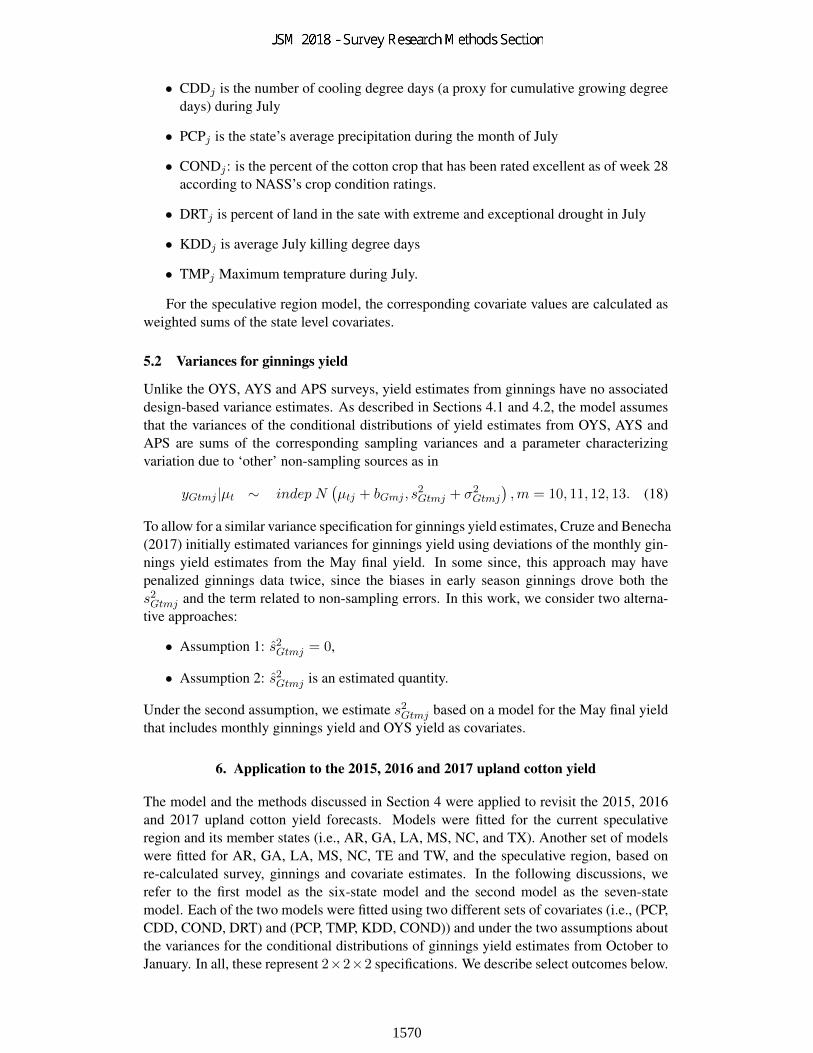
Table 1: Average percent absolute differences of model estimates from May yield

State 6-State Model 7-State ModelAugust Estimates

A 9.4 10.1B 2.5 3.6C 8.9 9.8D 22.3 24.0E 6.1 8.5F 7.6 8.6

SPEC 5.4 5.7January Estimates

A 1.2 1.2B 0.9 0.7C 1.7 2.1D 2.1 2.1E 2.7 2.8F 0.4 0.7

SPEC 0.8 0.8

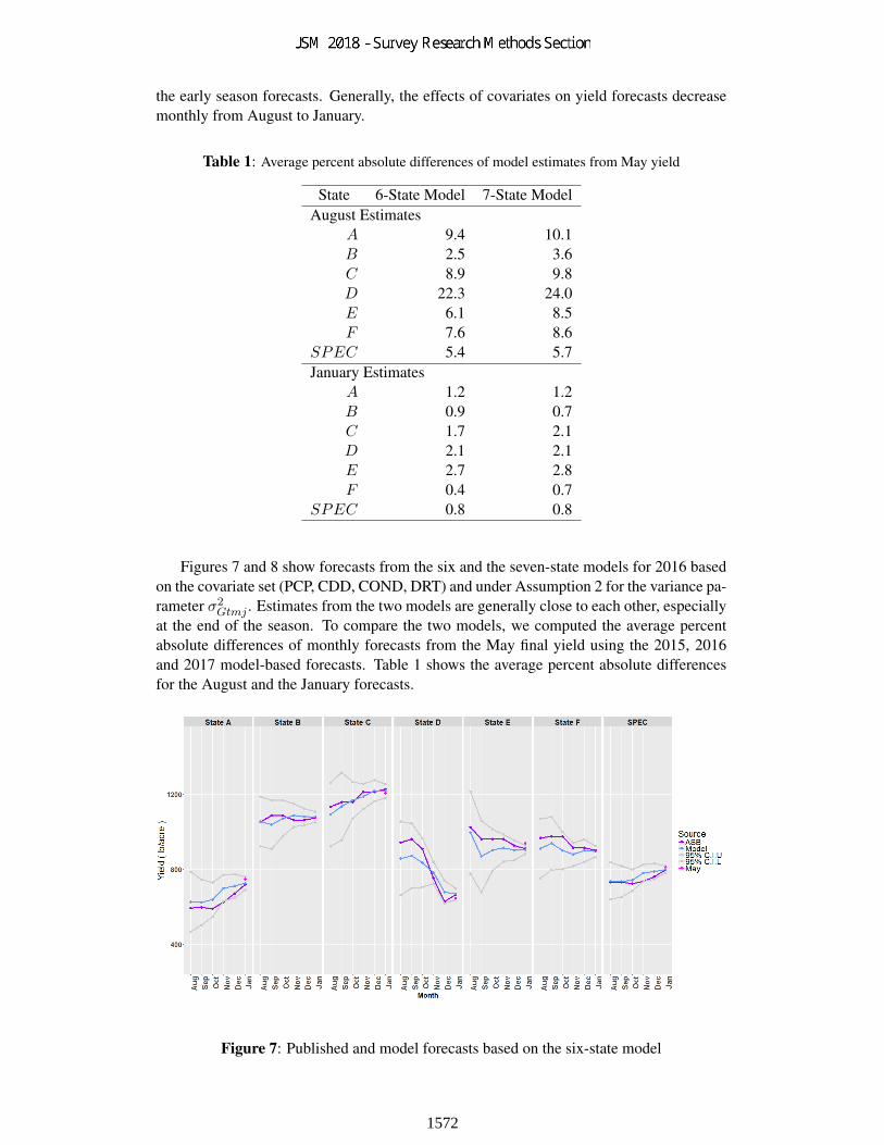
Figures 7 and 8 show forecasts from the six and the seven-state models for 2016 basedon the covariate set (PCP, CDD, COND, DRT) and under Assumption 2 for the variance pa-rameter σ2

Gtmj . Estimates from the two models are generally close to each other, especiallyat the end of the season. To compare the two models, we computed the average percentabsolute differences of monthly forecasts from the May final yield using the 2015, 2016and 2017 model-based forecasts. Table 1 shows the average percent absolute differencesfor the August and the January forecasts.

Figure 7: Published and model forecasts based on the six-state model

1572

Figure 8: Published and model forecasts based on the seven-state model

The absolute differences from the two models are close to each other, but the six-statemodel performed better for most states. Finally, the two assumptions about the variancefor the conditional distribution of ginnings yield were compared using the 2015, 2016 and2017 model-based forecasts and the corresponding standard errors for the six-state modelwith covariate set (PCP, CDD, COND, DRT).

Table 2: Ratio of model estimated SEs for yield forecasts from models that use and do notuse ginnings SEs

State 2015 2016 2017August Estimates

A 1.01 1.00 1.02B 0.94 0.97 0.96C 0.98 1.00 1.00D 0.94 0.97 0.98E 1.10 0.99 0.99F 0.97 0.95 0.96

SPEC 1.01 0.99 1.00

Generally, the two assumptions provided similar forecasts and standard errors for allstates and the speculative region, implying that we may not need to estimate samplingvariances for ginnings yield separately. Ratios of model estimated SEs from the modelunder Assumptions 1 and 2 are presented in Table 2.

7. Discussion

A Bayesian hierarchical model that combines historical and current data from multiple sur-veys, cotton ginnings and covariates to produce a single forecast for a region and its memberstates has been developed. The approach allows for the estimation of a reproducible yieldforecast with an associated measure of uncertainty. Because the current yield models for

1573

upland cotton and the other crops input data at state and regional levels, any within-stateheterogeneities in yield, production, and weather conditions may not be fully accountedfor when forecasts are produced. In an attempt to account for some heterogeneities andimprove yield forecasts, sub-state level data were incorporated in the model-based analysisfor the largest producing state, and comparisons were made between models that use statelevel data and models based on both state and sub-state level data. Comparisons of two as-sumptions for the variance of ginnings yield in the models showed little difference betweenthe two approaches, indicating that the model may be fitted without the need for inputingan estimated variance for ginnings yield from October to January. Upland cotton yield isaffected by a number of factors that can be incorporated into the model as covariates. Asmany of these covariates are related to weather conditions, an important task in selectingpredictors from a pool is determination of the week or month in which a potential covariatehas the highest impact on yield. In addition, determining the set of covariates that givesan optimal fit to the model is another important consideration. Preliminary attempts weremade to select the best set of covariates for the upland cotton model, but covariate selectionis still an ongoing research project.

Acknowledgements

The authors would like to thank Jared Pratt and several other USDA NASS MethodologyDivision staff for their knowledge and assitance in resummarizing an extended history ofsurvey data and data for sub-state divisions of Texas. We thank Clyde Fraisse, and AnaWagner of Univeristy of Florida for early access to smaller-than-state summaries of cli-matalogical variables derived from the AgroClimate tool. This research was supported inpart by the intramural research program of the U.S. Department of Agriculture, NationalAgricultural Statistics Service.

Disclaimer

The findings and conclusions in this preliminary publication have not been formally dis-seminated by the U.S. Department of Agriculture and should not be construed to representany agency determination or policy.

References

Adrian, D. (2012). A model-based approach to forecasting corn and soybean yields. Fourth InternationalConference on Establishment Surveys.

Cruze, N. B. (2015). Integrating survey data with auxiliary sources of information to estimate crop yields. InJSM Proceedings, Survey Research Methods Section. Alexandria, VA: American Statistical Association.

Cruze, N. B. (2016). A Bayesian Hierarchical Model for Combining Several Crop Yield Indications. In JSMProceedings, Survey Research Methods Section. Alexandria, VA: American Statistical Association.

Cruze, N. B. and Benecha, H. K. (2017). A Model-Based Approach to Crop Yield Forecasting. In JSMProceedings, Bayesian Statistical Science Section. Alexandria, VA: American Statistical Association.

Gelman, A., Carlin, J., Stern, H., and Rubin, D. (2003). Bayesian Data Analysis (2nd ed.). Chapman &Hall/CRC.

Ishwaran, H. and Rao, J. S. (2005). Spike and slab variable selection: frequentist and Bayesian strategies. TheAnnals of Statistics, 2:730773.

Nandram, B., Berg, E., and Barboza, W. (2014). A hierarchical Bayesian model for forecasting state-level cornyield. Environmental and Ecological Statistics, 21(3):507–530.

1574

Nandram, B. and Sayit, H. (2011). A Bayesian analysis of small area probabilities under a constraint. SurveyMethodology, 37:137–152.

Wang, J. C., Holan, S. H., Nandram, B., Barboza, W., Toto, C., and Anderson, E. (2012). A Bayesian approachto estimating agricultural yield based on multiple repeated surveys. Journal of Agricultural, Biological, andEnvironmental Statistics, 17(1):84–106.

1575