Unsteady waves in compressible ﬂow - Stanford...

Chapter 13

Unsteady waves in compressibleflow

13.1 Governing equations

One of the most important applications of compressible flow theory is to the analysis ofthe generation and propagation of sound. In Chapter 6 we worked out the equations forhomentropic, unsteady flow that are the starting point for the derivation of the acousticequations. For r⇥ U = 0, and rs = 0, the equations of motion are

@⇢

@t+

@

@xk(⇢Uk) = 0

⇢@Ui

@t+ ⇢

@

@xi

✓UkUk

2

◆+

@P

@xi= 0

P

P0

=

✓⇢

⇢0

◆�

.

(13.1)

The role of the energy equation is played by the isentropic relation between pressure anddensity.

13.2 The acoustic equations

Now consider an unsteady flow where disturbances in density and pressure are extremely

13-1

CHAPTER 13. UNSTEADY WAVES IN COMPRESSIBLE FLOW 13-2

small compared to constant background values.

⇢ = ⇢0

+ ⇢0 ;⇢0

⇢0

<< 1

P = P0

+ P 0 ;P 0

P0

<< 1

(13.2)

In addition, assume that the velocity field involves very small fluctuations about zero.Linearize (13.1) by dropping higher order nonlinear terms.

@⇢

@t+ ⇢

0

@Uk

@xk= 0

⇢0

@Ui

@t+

@P

@xi= 0

(13.3)

Now define the dimensionless density disturbance

r =⇢� ⇢

0

⇢0

. (13.4)

In terms of this variable the equations of motion become

@r

@t+

@Uk

@xk= 0

⇢0

@Ui

@t+

@P

@xi= 0

P

P0

= (1 + r)� ⇠= 1 + �r.

(13.5)

Slight rearrangement produces the acoustic equations

@r

@t+

@Uk

@xk= 0

@Ui

@t+ a

0

2

@r

@xi= 0

(13.6)

where


a0

2 = �P0

⇢0

. (13.7)

Now di↵erentiate the linearized continuity equation with respect to time and the linearizedmomentum equation with respect to space.

@2r

@t2+

@2Uk

@xk@t= 0

@2Uk

@xk@t+ a

0

2

@2r

@xk@xk= 0

(13.8)

Subtract one from the other in (13.8). The dimensionless density disturbance satisfies thelinear wave equation.

@2r

@t2� a

0

2

@2r

@xk@xk= 0 (13.9)

Now repeat the process with the di↵erentiation reversed. The result is

@2r

@t@xi+

@2Uk

@xk@xi= 0

@2Ui

@t2+ a

0

2

@2r

@xi@t= 0.

(13.10)

Again, subtract one equation from the other in (13.10). The velocity fluctuation satisfiesthe equation

@2Ui

@t2� a

0

2

@2Uk

@xk@xi= 0. (13.11)

Recall the vector identity r⇥�r⇥ U

�= r

�r · U

��r2U Using this identity and the fact

that the flow is irrotational, (13.11) can be expressed as the linear wave equation

@2Ui

@t2� a

0

2

@2Ui

@xk@xk= 0. (13.12)

Similarly, the pressure satisfies the wave equation. Substitute


r =1

�

✓P � P

0

P0

◆(13.13)

into (13.9)

@2P

@t2� a

0

2

@2P

@xk@xk= 0. (13.14)

Finally, the temperature also satisfies the wave equation.

@2T

@t2� a

0

2

@2T

@xk@xk= 0 (13.15)

13.3 Propagation of acoustic waves in one space dimension

In one dimensional flow the acoustic equations become

@r

@t+

@U

@x= 0

@Ui

@t+ a

0

2

@r

@x= 0.

(13.16)

The wave equation

@2r

@t2� a

0

2

@2r

@x2= 0 (13.17)

can be solved in a very general form

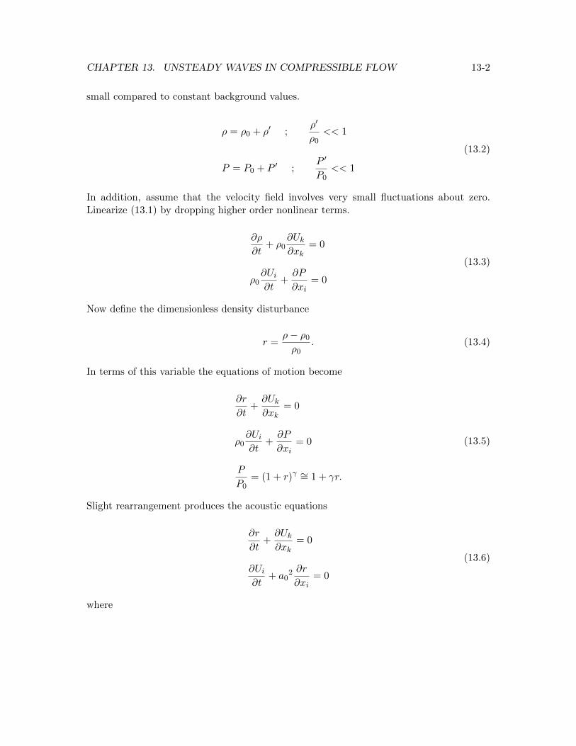
r (x, t) = F (x� a0

t) +G (x+ a0

t) (13.18)

where F and G are arbitrary functions. The character of the solution can be understoodby considering first the case G = 0. Figure 13.1 illustrates the evolution of an initialdistribution of F propagating to the right in the x� t plane.

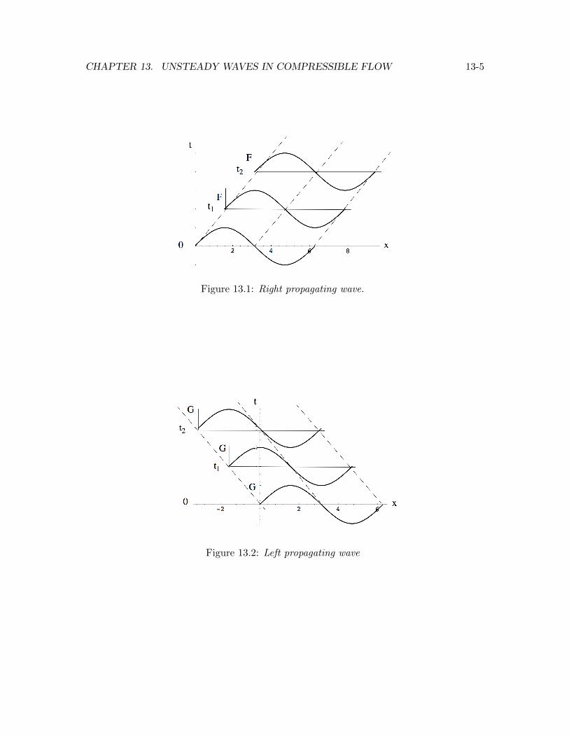
The disturbance moves to the right unchanged in shape. Acoustic waves are nondisper-sive meaning that the wave speed does not depend on the wavelength. The figure belowillustrates the evolution of an initial distribution of G propagating to the left in the x� tplane.


Figure 13.1: Right propagating wave.

Figure 13.2: Left propagating wave


In the absence of dispersion and dissipation, the waves simply translate while retaining theirform. The pressure disturbance produced by the wave is related to the density by

P � P0

P0

= �r = �

✓⇢� ⇢

0

⇢0

◆. (13.19)

In di↵erential form

dP

P= �

d⇢

⇢. (13.20)

The velocity induced by the acoustic disturbance can also be written in a very generalform.

U (x, t) = f (x� a0

t) + g (x+ a0

t) (13.21)

Substitute the expressions for r and U into the acoustic equations.

@

@t(F (x� a

0

t) +G (x+ a0

t)) +@

@x(f (x� a

0

t) + g (x+ a0

t)) = 0

@

@t(f (x� a

0

t) + g (x+ a0

t)) + a0

2

@

@x(F (x� a

0

t) +G (x+ a0

t)) = 0

(13.22)

Let

⇠ = x� a0

t

⌘ = x+ a0

t.(13.23)

Equation (13.22) becomes

�a0

F⇠ + a0

G⌘ + f⇠ + g⌘ = 0

a0

F⇠ + a0

G⌘ � f⇠ + g⌘ = 0.(13.24)

Add and subtract the relations in (13.24)

�a0

F⇠ + f⇠ = 0

a0

G⌘ + g⌘ = 0.(13.25)


From (13.25) we can conclude that g = �a0

G; f = a0

F . The result (13.25) gives us therelationship between density and velocity in left and right running waves.

U (x, t) = a0

F (x� a0

t)� a0

G (x+ a0

t) (13.26)

Now

U

a0

r=

F �G

F +G. (13.27)

In a right running wave

U

a0

r= 1. (13.28)

In a left running wave

U

a0

r= �1. (13.29)

In di↵erential form (13.27) is equivalent to

dU = ±a0

d⇢

⇢

dP

P= �

d⇢

⇢.

(13.30)

13.4 Isentropic, finite amplitude waves

The speed of sound may vary from one point to another and in a general, 1-D, isentropicflow.

a = a0

✓⇢

⇢0

◆ ��1

2

(13.31)

Locally, the particle disturbance velocity is given by (13.30) with the speed of sound re-garded as a function of space and time.


dU = ±ad⇢

⇢(13.32)

Equation (13.32) is one of the most important equations in unsteady gas dynamics and isoften introduced as an intuitively obvious extension of equation (13.30). We can put (13.32)on a firmer foundation by returning to the full nonlinear equations for one-dimensional,isentropic flow. In one dimension (13.1) becomes

@⇢

@t+ ⇢

@U

@x+ U

@⇢

@x= 0

@U

@t+ U

@U

@x+

�P0

⇢0

2

✓⇢

⇢0

◆��2 @⇢

@x= 0.

(13.33)

Now assume that the density can be written as a function of the velocity.

⇢ = ⇢ (U) (13.34)

The derivatives of the density are

@⇢

@t=

d⇢

dU

@U

@t

@⇢

@x=

d⇢

dU

@U

@x.

(13.35)

Substitute (13.35) into (13.33).

d⇢

dU

@U

@t+ ⇢

@U

@x+ U

d⇢

dU

@U

@x= 0

@U

@t+ U

@U

@x+

�P0

⇢0

2

✓⇢

⇢0

◆��2 d⇢

dU

@U

@x= 0

(13.36)

Rearrange (13.36).

@U

@t+ U

@U

@x+

⇢

d⇢/dU

@U

@x= 0

@U

@t+ U

@U

@x+

�P0

⇢0

2

✓⇢

⇢0

◆��2 d⇢

dU

@U

@x= 0

(13.37)


Comparing the continuity and momentum equation in (13.37) we see that in order for(13.34) to be a solution of (13.33) we must have

⇢

d⇢/dU=

�P0

⇢0

2

✓⇢

⇢0

◆��2 d⇢

dU. (13.38)

Equation (13.38) can be rearranged to read

✓d⇢

dU

◆2

=⇢0

2

a0

2

✓⇢

⇢0

◆3��

. (13.39)

Take the square root of (13.39).

d⇢

dU= ±⇢

0

a0

✓⇢

⇢0

◆ 3��2

(13.40)

Now substitute the isentropic relation between the speed of sound and density

a

a0

=

✓⇢

⇢0

◆ ��1

2

(13.41)

into (13.40). Equation (13.40) becomes

dU = ±ad⇢

⇢(13.42)

which confirms the general validity of (13.32). Using the isentropic assumption, (13.32)can be integrated from some initial state to a final state.

U = ±Z ⇢

⇢1

ad⇢

⇢= ±a

1

Z ⇢

⇢1

✓⇢

⇢1

◆ ��1

2 d⇢

⇢(13.43)

Integrating,

U = ± 2a1

� � 1

✓⇢

⇢1

◆ ��1

2

� 1

!= ± 2

� � 1(a� a

1

) . (13.44)

The local acoustic speed is


a = a1

±✓� � 1

2

◆U (13.45)

and the wave speed at any point is

c = a± U = a1

±✓� � 1

2

◆U ± U = a

1

±✓� + 1

2

◆U. (13.46)

13.5 Centered expansion wave

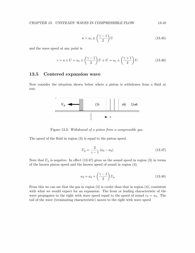
Now consider the situation shown below where a piston is withdrawn from a fluid atrest.

Figure 13.3: Withdrawal of a piston from a compressible gas.

The speed of the fluid in region (3) is equal to the piston speed.

Up =2

� � 1(a

3

� a4

) (13.47)

Note that Up is negative. In e↵ect (13.47) gives us the sound speed in region (3) in termsof the known piston speed and the known speed of sound in region (4).

a3

= a4

+

✓� � 1

2

◆Up (13.48)

From this we can see that the gas in region (3) is cooler than that in region (4), consistentwith what we would expect for an expansion. The front or leading characteristic of thewave propagates to the right with wave speed equal to the speed of sound c

4

= a4

. Thetail of the wave (terminating characteristic) moves to the right with wave speed


c3

= a3

+ Up = a4

+

✓� + 1

2

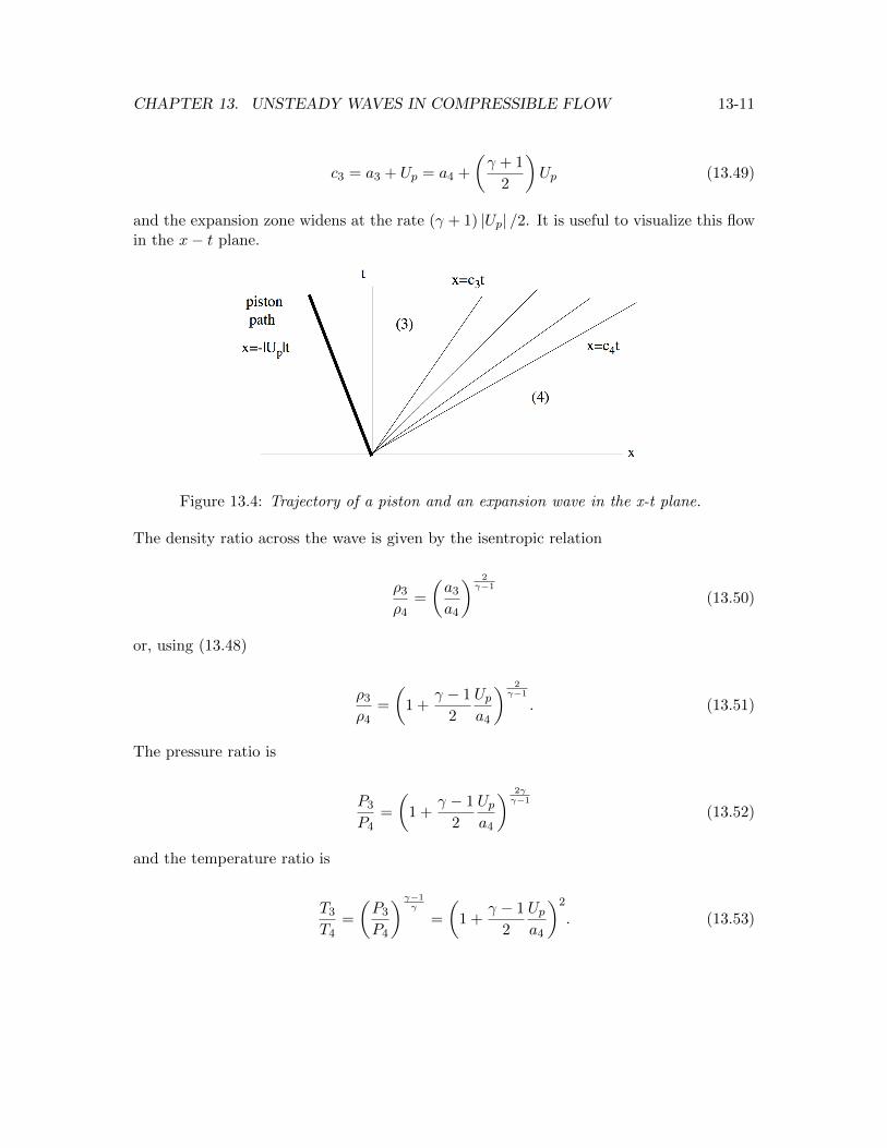
◆Up (13.49)

and the expansion zone widens at the rate (� + 1) |Up| /2. It is useful to visualize this flowin the x� t plane.

Figure 13.4: Trajectory of a piston and an expansion wave in the x-t plane.

The density ratio across the wave is given by the isentropic relation

⇢3

⇢4

=

✓a3

a4

◆ 2

��1

(13.50)

or, using (13.48)

⇢3

⇢4

=

✓1 +

� � 1

2

Up

a4

◆ 2

��1

. (13.51)

The pressure ratio is

P3

P4

=

✓1 +

� � 1

2

Up

a4

◆ 2��1

(13.52)

and the temperature ratio is

T3

T4

=

✓P3

P4

◆ ��1

�

=

✓1 +

� � 1

2

Up

a4

◆2

. (13.53)


In summary, our solution of the small disturbance wave equation from the previous sectionhas allowed us to determine all the properties of a finite expansion wave. Things workedout this way because the expansion wave is isentropic to a high degree of accuracy. Notethe similarity between the 1-D unsteady expansion wave and the steady Prandtl-Meyerexpansion, and the presence of space-time characteristics in the x � t plane along whichthe properties of the flow are constant.

13.6 Compression wave

Suppose the piston motion is to the right into the gas. None of the above relations changebut the physics does change and this can be seen from the x� t diagram.

Figure 13.5: Compression wave converging to a shock in the x-t plane.

The wave speed at the surface of the piston is

c2

= a2

+ Up = a1

+� + 1

2Up. (13.54)

In this case the characteristics tend to cross, at which point the isentropic assumption is nolonger valid. The system of compression waves catches up to itself (nonlinear steepening)in a very short time collapsing to form a shock wave.

13.7 The shock tube

A very important device used to study shock waves in the laboratory is the shock tubeshown schematically in figure 13.6.


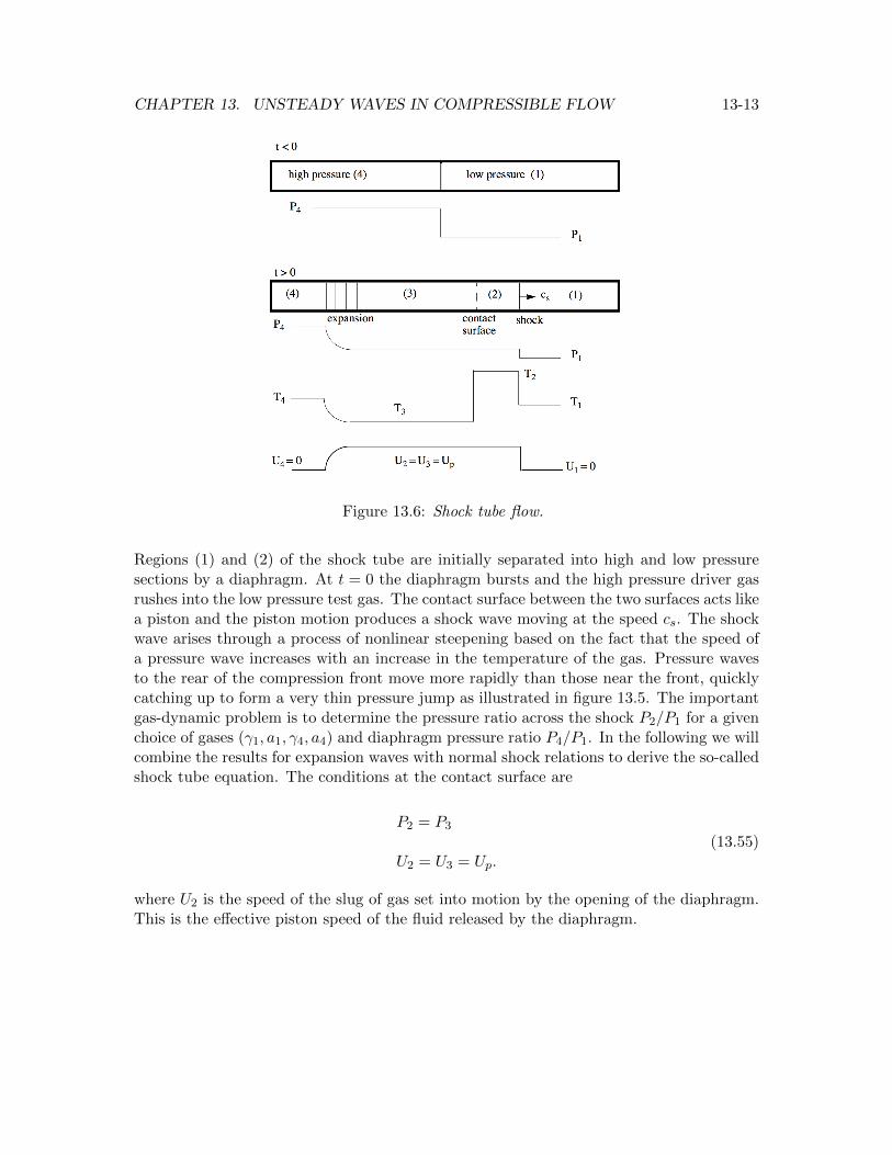
Figure 13.6: Shock tube flow.

Regions (1) and (2) of the shock tube are initially separated into high and low pressuresections by a diaphragm. At t = 0 the diaphragm bursts and the high pressure driver gasrushes into the low pressure test gas. The contact surface between the two surfaces acts likea piston and the piston motion produces a shock wave moving at the speed cs. The shockwave arises through a process of nonlinear steepening based on the fact that the speed ofa pressure wave increases with an increase in the temperature of the gas. Pressure wavesto the rear of the compression front move more rapidly than those near the front, quicklycatching up to form a very thin pressure jump as illustrated in figure 13.5. The importantgas-dynamic problem is to determine the pressure ratio across the shock P

2

/P1

for a givenchoice of gases (�

1

, a1

, �4

, a4

) and diaphragm pressure ratio P4

/P1

. In the following we willcombine the results for expansion waves with normal shock relations to derive the so-calledshock tube equation. The conditions at the contact surface are

P2

= P3

U2

= U3

= Up.(13.55)

where U2

is the speed of the slug of gas set into motion by the opening of the diaphragm.This is the e↵ective piston speed of the fluid released by the diaphragm.


In a frame of reference moving with the shock wave the gas velocities are

U 01

= �cs

U 02

= �cs + Up

(13.56)

and the shock jump conditions are

U 02

U 01

=1 + �

1

�1

2

M1

2

�1

+1

2

M1

2

P2

P1

=�1

M1

2 � �1

�1

2

�1

+1

2

(13.57)

where M1

= cs/a1 = �U 01

/a1

. Using the first relation in (13.57) we can write

U 02

� U 01

U 01

=1 + �

1

�1

2

M1

2

�1

+1

2

M1

2

� 1 =1�M

1

2

�1

+1

2

M1

2

. (13.58)

The piston velocity is

Up = U 02

� U 01

= U 01

0

@ 1�M1

2

�1

+1

2

M1

⇣�U 0

1

a1

⌘

1

A = a1

M

1

2 � 1�1

+1

2

M1

!. (13.59)

Note that Up is positive. Using the second relation in (13.57), equation (13.59) can beexpressed in terms of the shock pressure ratio as

Up = a1

✓P2

P1

� 1

◆0

@ 2

�1

(�1

+ 1)⇣P2

P1

⌘+ �

1

(�1

� 1)

1

A1/2

. (13.60)

Equation (13.60) is the expression for the piston velocity derived using normal shock theory.Now lets work out an expression for the piston velocity using isentropic expansion theory.The velocity behind the expansion is

U3

= Up =2a

4

�4

� 1

1�

✓P3

P4

◆ �4

�1

2�4

!. (13.61)


Equate (13.60) and (13.61).

a1

✓P2

P1

� 1

◆0

@ 2

�1

(�1

+ 1)⇣P2

P1

⌘+ �

1

(�1

� 1)

1

A1/2

=2a

4

�4

� 1

1�

✓P3

P2

P2

P1

P1

P4

◆ �4

�1

2�4

!

(13.62)

Using the following identity

P3

P4

=P3

P2

P2

P1

P1

P4

(13.63)

and noting that P3

/P2

= 1 solve (13.61) for P4

/P1

= 1. The result is the basic shock tubeequation

P4

P1

=P2

P1

0

B@1�(�

4

� 1)⇣a1

a4

⌘⇣P2

P1

� 1⌘

⇣4�

1

2 + 2�1

(�1

+ 1)⇣P2

P1

� 1⌘⌘

1/2

1

CA

�⇣

2�4

�4

�1

⌘

(13.64)

plotted in figure 13.7. Given (P4

/P1

, �1

, �4

, a1

, a4

) we can determine the shock strengthP2

/P1

from (13.64).

Figure 13.7: Shock tube pressure ratio versus shock strength.

Once the shock strength is determined, the shock Mach number can be determined from


P2

P1

=2�

1

�1

+ 1Ms

2 �✓�1

� 1

�1

+ 1

◆(13.65)

or

Ms2 =

�1

+ 1

2�1

✓P2

P1

+�1

� 1

�1

+ 1

◆. (13.66)

Notice that very large values of P4

/P1

are required to generate strong shocks. One wayto improve the performance of the shock tube is to select a driver gas with a large speedof sound. Helium driving into nitrogen will produce a much stronger shock wave than sayArgon driving into nitrogen at a given P

4

/P1

. In essence Helium provides a much lighterpiston that can translate much more rapidly into the test gas. The figure below providesthis comparison.

Figure 13.8: Shock Mach number for several driver gases.

Hydrogen as the driver gas produces the strongest shock waves however the fire and explo-sion hazard involved has limited its use.

13.7.1 Example - flow induced by the shock in a shock tube

The flow in a shock tube is shown below.

The shock wave induces a gas velocity in the laboratory frame, Up = U2

= U3

where


Figure 13.9: Flow induced in a shock tube.

U2

= a1

✓P2

P1

� 1

◆0

@ 2

�1

(�1

+ 1)⇣P2

P1

⌘+ �

1

(�1

� 1)

1

A1/2

. (13.67)

Suppose the gas in the driver section and test section is Air initially at 300K. A shockwave with a Mach number of 2 is produced in the tube.

1) Determine the stagnation temperature of the gas in region (2) in the laboratory frame.

2) Determine the stagnation temperature of the gas in region (3) in the laboratory frame.

Answer

The pressure ratio across a Mach number 2 shock in air is

P2

P1

= 4.5 (13.68)

and the temperature ratio is

T2

T1

= 1.687. (13.69)

The speed of sound in air is a1

=p�RT = 347m/sec and the heat capacity at constant

pressure is, Cp = 1005m2/sec2 �K. The piston velocity is

U2

= a1

✓P2

P1

� 1

◆0

@ 2

�1

(�1

+ 1)⇣P2

P1

⌘+ �

1

(�1

� 1)

1

A1/2

=

347⇥ 3.5⇥✓

2

15.68

◆1/2

= 433.75m/sec

. (13.70)


The temperature in region (3) is obtained from (13.53).

T3

T4

=

✓1 +

� � 1

2

Up

a4

◆2

=

✓1� 0.2

✓433.75

347

◆◆2

= 0.5625 (13.71)

Now, in region (2)

Tt2 = T2

+1

2

Up2

Cp= 1.687⇥ 300 +

433.752

2⇥ 1005= 506.1 + 93.6 = 599.7K (13.72)

and in region (3)

Tt3 = T3

+1

2

Up2

Cp= 0.5625⇥ 300 +

433.752

2⇥ 1005= 168.75 + 93.6 = 262.35K. (13.73)

13.8 Problems

Problem 1 - Consider the expression ⇢Un, n = 1 corresponds to the mass flux, n =2 corresponds to the momentum flux and n = 3 corresponds to the energy flux of acompressible gas. Use the acoustic relation

dU = ±ad⇢

⇢(13.74)

to determine the Mach number (as a function of n) at which ⇢Un is a maximum in aone-dimensional, unsteady expansion wave. The steady case is considered in one of theproblems at the end of Chapter 9.

Problem 2 - In the shock tube example discussed above, determine the stagnation pressureof the gas in regions (2) and (3). Determine the stagnation pressure in both the laboratoryframe and in the frame of reference moving with the shock wave.

Problem 3 - Figure 13.10 below shows a sphere moving over a flat plate in a ballisticrange. The sphere has been fired from a gun and is translating to the left at a Machnumber of 3. The static temperature of the air upstream of the sphere is 300K and thepressure is one atmosphere. On the plane of symmetry of the flow (the plane of the photo)the shock intersects the plate at an angle of 25 degrees as indicated.

i) Determine the flow Mach number, speed and angle behind the shock in region 2 close tothe intersection with the plate. Work out your results in a frame of reference moving with


Figure 13.10: Sphere moving supersonically over a flat plate.

the sphere. In this frame the upstream air is moving to the right at 3 times the speed ofsound.

ii) What are the stream-wise and plate normal velocity components of the flow in region 2referred to a frame of reference at rest with respect to the upstream gas.

iii) Determine the stagnation temperature and pressure of the flow in region 2 referred toa frame of reference at rest with respect to the upstream gas.

Problem 4 - We normally think of the shock tube as a device that can be used to studyrelatively strong shock waves. But shock tubes have also been used to study weak shocksrelevant to the sonic boom problem. Suppose the shock tube is used to generate weakshock waves with P

2

/P1

= 1 + ". Show that for small " the relationship between P2

/P1

and P4

/P1

is approximated by

P4

P1

= 1 +A". (13.75)

How does A depend on the properties of the gases in regions 1 and 4? Use the exact theoryto determine the strength of a shock wave generated in an air-air shock tube operated atP4

/P1

= 1.2. Compare with the approximate result.

Problem 5 - The sketch below shows a one meter diameter tube filled with air and dividedinto two volumes by a heavy piston of weightW . The piston is held in place by a mechanicalstop and the pressure and temperature are uniform throughout the tube at one atmosphereand 300K. Body force e↵ects in the gas may be neglected.


Figure 13.11: Gravity driven frictionless piston in a shock tube.

The piston is released and accelerates downward due to gravity. After a short transientthe piston reaches a constant velocity Up. The piston drives a shock wave ahead of it ata wave speed cs equal to twice the sound speed in region 1. What is the weight of thepiston?

Problem 6 - Each time Stanford makes a touchdown an eight inch diameter, open endedshock tube is used to celebrate the score. Suppose the shock wave developed in the tubeis required to have a pressure ratio of 2. What pressure is needed in the driver section?Assume the driver gas is air. What is the shock Mach number? Suppose the shock tube ismounted vertically on a cart as shown in figure 13.12 below. Estimate the force that thecart must withstand when the tube fires.

Figure 13.12: Shock tube mounted on a cart.

Problem 7 - In figure 13.13 a moveable piston sits in the middle of a long tube filled withair at one atmosphere and 300K. At time zero the piston is moved impulsively to the rightat Up = 200m/sec.

1) What is the pressure on the right face of the piston (region 2) in atmospheres?


Figure 13.13: Frictionless piston in a shock tube.

2) What is the pressure on the left face of the piston (region 3) in atmospheres?

Problem 8 - One of the most versatile instruments used in the study of fluid flow is theshock tube. It can even be used as a wind tunnel as long as one is satisfied with short testtimes. Figure 13.14 below illustrates the idea. An airfoil is placed in the shock tube andafter the passage of the shock it is subject to flow of the test gas at constant velocity Up

and temperature T2

. In a real experiment the contact surface is quite turbulent and so thepractical usefulness of the flow is restricted to the time after the arrival of the shock andbefore the arrival of the contact surface, typically a millisecond or so.

Figure 13.14: Shock tube used as a wind tunnel.

Proponents of this idea point out that if the shock Mach number is very large the flow overthe body can be supersonic as suggested in the sketch above.

1) Show that this is the case.

2) For very large shock Mach number, which test gas would produce a higher Mach numberover the body, helium or air. Estimate the Mach number over the body for each gas.

Problem 9 - Figure 13.15 below shows a shock wave reflecting from the endwall of a shocktube. The reflected shock moves to the left at a constant speed crs into the gas that wascompressed by the incident shock. The gas behind the reflected shock, labeled region (5),is at rest and at a substantially higher temperature and pressure than it was in state (1)before the arrival of the incident shock.

1) Suppose the gas in the driver and test sections is helium at an initial temperature of300K prior to opening the diaphragm. The Mach number of the incident shock wave is 3.


Figure 13.15: Shock wave reflecting from an end wall.

Determine the Mach number of the reflected shock.

2) Determine T5

/T1

.

Problem 10 - One of the key variables in the design of a shock tube is the length neededfor a shock to develop from the initial compression process. Suppose a piston is used tocompress a gas initially at rest in a tube. During the startup transient 0 < t < t

1

the pistonspeed increases linearly with time as shown on the x� t diagram in figure 13.16.

Figure 13.16: Piston compressing air.

In a shock tube the startup time t1

is generally taken to be the time required for thediaphragm to open. Let the gas be air at T

1

= 300K. Use t1

= 5 ⇥ 10�3sec and A =4⇥ 104m/sec2 to estimate the distance needed for the shock wave to form.

Unsteady waves in compressible ﬂow - Stanford...

Documents

Transcript of Unsteady waves in compressible ﬂow - Stanford...