UNIVERSITAT POLITÈCNICA DE CATALUNYA BARCELONA TECH
161
UNIVERSITAT POLITÈCNICA DE CATALUNYA BARCELONA TECH Departament d’Eginyeria Civil i Ambiental Laboratori d’Enginyeria Marítima Programa de Doctorat en Ciències del Mar THESIS BY COMPENDIUM OF PUBLICATIONS PhD Thesis presented by Felícitas Calderón Vega For the degree of DOCTOR DIRECTED BY: Dr. César Mosso Aranda Dr. Adrián David García Soto Barcelona, Febrero, 2020 Probabilistic characterization of single and concurrent metocean variables of Mexican coasts with seasonal variability using extreme value theory, with application to reliability of coastal structures
Transcript of UNIVERSITAT POLITÈCNICA DE CATALUNYA BARCELONA TECH

UNIVERSITAT POLITÈCNICA DE CATALUNYA BARCELONA TECH
Departament d’Eginyeria Civil i Ambiental Laboratori d’Enginyeria Marítima
Programa de Doctorat en Ciències del Mar
THESIS BY COMPENDIUM OF PUBLICATIONS
PhD Thesis presented by
Felícitas Calderón Vega
For the degree of DOCTOR
DIRECTED BY:
Dr. César Mosso Aranda
Dr. Adrián David García Soto
Barcelona, Febrero, 2020
Probabilistic characterization of single and concurrent
metocean variables of Mexican coasts with seasonal
variability using extreme value theory, with application
to reliability of coastal structures

1
DEDICATORIA
A Arlene Damara, Aldair Daniel y Adrián David.
Mis hijos, mi motor de vida.
Y a David
Mi amado esposo
To Arlene Damara, Aldair Daniel and Adrián David
My kids, the energy of my life.
And to David
Mi beloved husband

2
CONTENTS
Abstract------------------------------------------------------------------------
Resumen-----------------------------------------------------------------------
Acknowledgments------------------------------------------------------------
I. THESIS BODY-----------------------------------------------------
1. Introduction-----------------------------------------------------------
1.1 Motivation---------------------------------------------------------
1.2 Objectives----------------------------------------------------------
1.3 Outline-------------------------------------------------------------
2. Background ------------------------------------------------------------
2.1 Characterization of Metocean Variables with Time-Dependent
GEV Models --------------------------------------------------------
2.1.1 Extreme Value Theory--------------------------------------
2.1.2 Extreme Time-Dependent GEV Distribution--------------
2.1.3 Inclusion of Seasonality------------------------------------
2.1.4 Fitting Technique-------------------------------------------
2.1.5 Assessment of the Uncertainty-----------------------------
2.1.6 Selection of the Model -------------------------------------
2.1.7 Verification of the Model ----------------------------------
2.1.8 Return Periods----------------------------------------------
2.2 Lineal Regression, Correlation and Residuals---------------------
2.3 Basic Concepts of Reliability Theory ------------------------------
2.3.1 Reliability Analysis-----------------------------------------
2.3.2 Cornell Reliability Index-----------------------------------
2.3.3 First-Order Second-Moment Reliability Index-----------
2.3.4 The Hasofer and Lind Reliability Index-------------------
2.3.5 First Order Reliability Method (FORM)------------------
2.3.6 Monte Carlo Simulation -----------------------------------
3. Overall Discussion and General Conclusions--------------------------
3.1 Conclusions---------------------------------------------------------
3.2 Future Research----------------------------------------------------
4. References---------------------------------------------------------------
4.1 References Paper A-------------------------------------------------
4
6
8
9
10
11
12
12
14
14
14
15
16
17
18
20
21
21
22
25
25
27
28
29
31
33
35
35
39
41
43

3
4.2 References Paper B--------------------------------------------------
4.3 References Paper C-------------------------------------------------
4.4 References Paper D-------------------------------------------------
4.5 References Book Chapter 1-----------------------------------------
4.6 References Book Chapter 2-----------------------------------------
II. COMPENDIUM OF PAPERS--------------------------------------
Paper A--------------------------------------------------------------
Paper B--------------------------------------------------------------
Book Chapter 1------------------------------------------------------
Book Chapter 2-----------------------------------------------------
APPENDIX ---------------------------------------------------------------------
Paper C-------------------------------------------------------------
Paper D-------------------------------------------------------------
46
48
50
52
54
56
57
82
104
116
130
131
143

4
Abstract
This thesis encompasses a set of different subjects related to metocean variables but
studied from different perspectives. The metocean variables are mainly significant wave
heights and wind velocities and, to a lesser extent, wave periods. The extreme value
theory is used to probabilistically characterized the metocean variables by means of the
generalized extreme value distribution (GEV). The effect of seasonality is included by
considering monthly maxima and using harmonic and subharmonic functions (i.e., time
dependency in the GEV model is incorporated). Although Mexican information was not
available to this study, the studies are considered applicable to Mexican coasts in the
Gulf of Mexico and the Pacific, since available public information from U.S. buoys
located in the Atlantic and Pacific oceans relatively close to the Mexican coasts is
employed. For the Pacific region, the GEV model accounting for seasonality is applied to
data from a buoy (this is reported in an article in the appendix and summarized as a book
chapter in the compendium of publications) and comparisons are carried out versus
analogous results for buoys in the Gulf of Mexico obtained in a previous study (included
also in the appendix). In other part of the thesis (another book chapter in the
compendium), but also for the buoy in the Pacific Ocean, a study is carried out to assess
the impact of including or excluding an atypical wave height in the seasonality and in
future projections (i.e., wave heights associated with given return periods), since an
atypically large significant wave heigh was observed for the considered buoy. One more
study (an article in the compendium) introduces the wind velocity as a Metocean
variable to be characterized with the time-dependent GEV model from data of a buoy in
the Gulf of Mexico. This wind velocity is not for monthly maxima, but for the recorded
wind velocity which simultaneously occurred with the maximum significant wave
heights, thus it is also referred to as companion wind in this work. It is pointed out that
the level of resolution is within that corresponding to the National Oceanic and
Atmospheric Administration (NOAA) from US, where the significant wave height and
wind speeds are denoted as WVHT and WSPD, respectively. The wind velocity is
averaged over an eight-minute period recorded at 3.6 m above sea level and the significant
wave height (the average of the highest one-third of all of the wave heights) over a 20-
minute period. For the scope of this study, these metocean variables are used as directly
given in the NOAA data. It is acknowledged that there may be a slight time lag between
the occurrence of one measurement and the other (since the averaging sampling periods

5
differ) but the difference is not considered significant for practical purposes; besides, we
are limited to the resolution of the available data. Nevertheless, the uncertainty and
impact of these different sampling periods in the projections are recommended as future
research subjects. This allowed to propose a simplified approach to determined
concurrent significant wave heights and associated wind velocities for given return
periods, while accounting for seasonality and quantitatively establishing the uncertainty
in the correlated metocean variables in question. This proposal can be potentially used
for design and engineering purposes, if the metocean are considered as hazards which
imposed demands on coastal (and structural) engineering systems. Additionally, the
effect of varying the considered time window for the extreme projections is explored. In
a final study (also an article in the compendium), an introduction to the reliability of
coastal (and also structural) engineering systems is presented; a breakwater is used as
case-study. The coastal structure is subjected to the action of wave heights with different
wave periods, for which the joint Longuet-Higgins distribution is used, and the
overtopping probability of failure is computed by using classical and revisited reliability
approaches. Future studies could combine the characterization of metocean variables as
time-dependent GEV models and the used reliability approaches to further investigate
the reliability of coastal and offshore systems.

6
Resumen
Esta tesis abarca diferentes temas relacionados con variables meteoceanográficas
(metocean) pero estudiadas desde diversas perspectivas. Estas variables son
principalmente el oleaje significativo y la velocidad de viento, y en menor medida el
período de oleaje. Se emplea la teoría de valores extremos para caracterizar
probabilísticamente las variables meteoceanográficas mediante el uso de la distribución
de extremos generalizada (GEV, por sus siglas en inglés), incluyendo el efecto de la
estacionalidad al considerar valores máximos mensuales, así como funciones armónicas
y subarmónicas, lo que significa que el modelo GEV es función del tiempo. Aunque no se
contó con información mexicana para el presente trabajo, se considera que lo
desarrollado aquí puede aplicarse a las costas mexicanas, ya que se usaron datos de boyas
estadounidenses situadas en los océanos Atlántico y Pacífico y relativamente cercanas a
costas mexicanas. Para la región del Pacífico se aplica el modelo GEV a una boya (esto se
describe en un artículo en el apéndice y resumido como capítulo de libro en el compendio
de publicaciones) y los resultados se comparan con resultados análogos de un estudio
previo, pero para boyas localizadas en el Golfo de México (dicho estudio también está
contenido en el apéndice). En otra parte de la tesis, pero también para la boya del Pacífico
(otro capítulo de libro en el compendio), mediante un estudio se estima el impacto de
incluir o excluir un dato atípico de la altura de oleaje en la estacionalidad y proyecciones
a futuro (i.e., las alturas de oleaje asociadas a periodos de retorno dados), ya que se
observó una ola atípicamente alta para la boya considerada. Un estudio más (un artículo
del compendio) incorpora a las velocidades de viento como variable mete-oceanográfica
para también caracterizarla como un modelo GEV que depende del tiempo, con datos de
una boya situada en el Golfo de México. Estas velocidades de viento no corresponden a
las máximas reportadas en cada mes, sino a aquellas que ocurrieron simultáneamente con
las máximas alturas significativas generadas por oleaje, por lo tanto, en este trabajo
también se le denota como viento acompañante (companion wind). Cabe resaltar que el
nivel de resolución empleado es el correspondiente al de la Administración Nacional
Oceánica y Atmosférica (NOAA por sus siglas en inglés), donde la altura de ola
significativa y las velocidades de viento se denotan como WVHT y WSPD,
respectivamente. La velocidad de viento se promedia para un periodo de 8 minutos y se
registra a 3.6 m sobre el nivel del mar y la altura de ola significativa (el promedio del tercio
superior de todas las alturas de ola) para un periodo de 20 minutos. Para los alcances de

7
este estudio, estas variables meteoceanográficas se toman directamente como están
reportadas en los datos de la NOAA. Se reconoce que puede haber un ligero desfase de
tiempo entre las mediciones de una variable y la otra (ya que los tiempos de muestreo
para el promedio son distintos) pero no se considera que esta diferencia sea significativa
para fines prácticos; además, estamos limitados a la resolución de los datos disponibles.
No obstante, la incertidumbre y el impacto de estos diferentes periodos de muestreo en
las proyecciones son consideradas como materias de investigación para futuros
proyectos. Esto conllevó a proponer un método simplificado para determinar alturas de
oleaje significativo concurrentes con los vientos asociados a la misma boya y tiempo y
para un periodo de retorno dado, y al mismo tiempo incorporando efectos de
estacionalidad y estableciendo de manera cuantitativa la incertidumbre para las variables
correlacionadas mencionadas. Esta propuesta es potencialmente útil para propósitos de
diseño e ingenieriles, si las variables meteoceanográficas se consideran como peligros que
imponen demandas a sistemas de ingeniería costeros (y estructurales). Adicionalmente,
se explora el efecto de utilizar diferentes ventanas de tiempo en las proyecciones de
valores extremos. En un estudio final (también un artículo del compendio) se presenta
una introducción a la confiabilidad de sistemas de ingeniería costera (y también
estructural), usando un rompeolas como caso de estudio. La estructura costera se somete
a la acción de oleaje con diferentes periodos, mediante el uso de la distribución de
Longuet-Higgins, y se calculan las probabilidades de falla por rebase aplicando métodos
de confiabilidad clásicos, y otros métodos consultados en retrospectiva y reconsiderados
prospectivamente. Estudios futuros podrían combinar el uso de modelos GEV como
función del tiempo para caracterizar variables meteoceanográficas con el uso de métodos
de confiabilidad, para investigar más a fondo la confiabilidad de sistemas costeros y costa
afuera.

8
Acknowledgments
The financial support from the Erasmus Mundus Coastal and Marine Engineering
and Management (CoMEM) programme is gratefully acknowledged. I thank
Laboratori d’Enginyeria Marítima, Universitat Politècnica de Catalunya and
Universidad de Guanajuato. I am also very thankful to Sonja Marie Ekrann Hammer
and Ø. Arntsen for their assistance through the Erasmus Mundus CoMEM
programme procedure. I am gratefully to my supervisors César Mösso and David
García for their patience and guidance. I am thankful to the externals revisors Rafael
Ramirez Mendoza and Andrés Rodriguez for their time and valuables suggestions
to improve this work. Thanks go to Rosa María Olea, Genoveva Comas and the
administrative staff of UPC for their help. I also thank my family, friends and
everyone who directly or indirectly help me to achieve this goal.

9
I. THESIS BODY

10
1. Introduction
Metocean variables as the wave height, wave period, the wind velocity which occurs
simultaneously with the previous variables, among others, should be
probabilistically characterized if they are to be used for the design and operation of
coastal and marine infrastructure and for other engineering applications. The
seasonal variation of extreme values for such metocean variables also affects the
planning, design, construction, operation and maintenance of shore and offshore
structures such as breakwaters, ports, oil facilities, etc. Moreover, values of
metocean variables should be oft associated with return periods usually employed
in codified design for practical applications. Furthermore, these seasonal wave
heights and wind velocities act together, as adding demands, over maritime and
structural systems which capacities must withstand the effects imposed by these
uncertain metocean variables.
Other aspects as the possible influence of atypical large values in the estimation of
extreme values, differences dependent on the considered region and even on the
considered site (for example at two different oceans as the Pacific and the Atlantic,
or two different locations within the same ocean), and the consideration of different
time windows in the extreme value projections for given return periods can also be
of interest to the researchers and designers.
Therefore, an adequate probabilistic characterization of the metocean variables, not
only as single demands but also as concurrent demands, is important for research
and practical purposes. For instance, the demands represented as probability
distributions could be used, together with the capacity of coastal structures ad
systems (which can be deterministic or probabilistic), to compute the probability of
failure of such structures and systems. This is important for codified design.

11
1.1 Motivation
In general, metocean variables are related to phenomena relevant to researchers of
several fields. Specifically, wind together with waves are metocean variables
capable of substantially impact ports, maritime structures and offshore facilities,
among other systems. The influen ce of these metocean variables is of great interest
to researchers, engineers and decision makers, because they influence the planning,
design, building, operation, maintenance and even decommission of important
projects. This is the case for ultimate limit states but also for serviceability limit
states. The former are important to prevent major failures of the above referred
systems and the latter to keep the systems functional. These limit states are usually
included in standards and guidelines, where also design criteria and acceptable
safety and functionality limits are established.
Since the metocean variables can be considered as random demands imposed to
systems which capacities must withstand such demands, for prescribed acceptable
levels contained in codes and regulations, it is desirable to characterize such
variables probabilistically. Also, operability and maintenance, among other issues,
could depend on the seasonality of metocean variables. Moreover, these variables
often do not act as single demands, but they act simultaneously on offshore facilities,
coastal structures and other engineering systems, that are designed for extreme
values associated to return periods. Consequently, it is of interest to inspect the
correlation of variables as wave height and wind velocity associated with a
prescribed return period. Extreme value theory is a key tool to investigate metocean
variables associated with given return periods, and classic probabilistic techniques
as regression and residual analysis can be also very useful tools. Among the
probability distributions contained within the extreme value theory, the generalized
extreme value distribution (GEV) is a powerful alternative since it encompasses the
three well-known extreme value distributions in a single mathematical expression.
Other aspects that could also be of interest for research and engineering purposes
include, but are not limited to, the influence of the atypical values and considered
time windows in extreme value projections, as well as regional and site to site
differences in extrapolation of extreme values useful for design. The previous issues
encourage the probabilistic characterization of metocean variables as, both, single

12
and concurrent acting random phenomena considering seasonality and using
extreme value theory. Furthermore, this characterization could be used to compute
the probability of failure of costal systems by using reliability theory.
1.2 Objectives
The objectives of the present study are to probabilistically characterize individual
metocean variables (significant wave height and wind velocity) by using a GEV
model and considering seasonality, also to develop a simple approach for
determining concurrent metocean variables with seasonal variation (significant
wave height and wind velocity) associated with given return periods by combining
GEV models and classical regression and to inspect the influence of atypical values,
considered time windows and a selected site in the projections of extreme values.
Other objective is to introduce the use of reliability theory to compute the
probability of failure of coastal structures.
1.3 Outline
This thesis is structured in two parts. First, the Thesis body, which summarises the
thesis work. Second, the Compendium of papers, which provides the details of the
study.
The background information is given in Section 2. Sub-section 2.1 describes the
probability methods developed and employed, and Sub-section 2.2 outlines the
lineal regression, correlation and residual analysis. In Sub-section 2.3 reliability
theory is briefly summarized, and the overall discussion and general conclusions are
given the section 4.
The compendium of papers is composed by two papers (Paper A and Paper B) and
two book chapters (Book chapter 1 and Book chapter 2). The two papers are already
published in international peer-reviewed journals. Other two papers are not part of
the main body of the Thesis (Paper C and Paper D), but they are included in an
appendix since they provide support to the work. All of them are listed below and
enclosed after the Thesis Body.
Paper A. Correlation of Concurrent Extreme Metocean Hazards Considering
Seasonality. Applied Sciences. Appl. Sci. 2020, 10, 4794; doi:10.3390/app10144794.

13
[Felícitas Calderón-Vega, Adrián-David García-Soto and César Mösso]
Paper B. Revisiting Two Simulation‐Based Reliability Approaches for Coastal and
Structural Engineering Applications. Applied Sciences. Appl. Sci. 2020, 10, 8176;
doi:10.3390/app10228176
[Adrián‐David García‐Soto, Felícitas Calderón‐Vega, César Mösso, Jesús‐Gerardo
Valdés‐Vázquez and Alejandro Hernández‐Martínez]
Book Chapter 1. Emerging Issues in Science and Technology Vol. 1. Chapter 11,
Influence of an Atypical Value in the Extreme Wave Analysis Using Non-Stationary
GEV Models. Print ISBN: 978-93-89562-66-8, eBook ISBN: 978-93-89562-67-5. DOI:
10.9734/bpi/eist/v1
[F. Calderón-Vega, C. Mösso and A. D. García-Soto]
Book Chapter 2. New Ideas Concerning Science and Technology. Describing the
Summary of Single Site Extreme Wave Analysis in the Pacific Ocean Comparing
Stationary and Non-Stationary GEV Models DOI:
https://doi.org/10.9734/bpi/nicst/v4/2310E [F. Calderón-Vega, C. Mösso, A. D.
García-Soto and E. Delgadillo-Ruiz]
Paper C. Single Site Extreme Wave Analysis in the Pacific Ocean Comparing
Stationary and Non-stationary GEV Models. Curr ent Journal of Applied Science and
Technology. 32(6): 1-12, 2019; Article no. CJAST.47420 [F. Calderón-Vega, C. Mösso,
A. D. García-Soto and E. Delgadillo-Ruiz]
Paper D. Analysis of extreme waves with seasonal variation in the Gulf of Mexico
using a time-dependent GEV model. Ocean Engineering. Ocean Engineering 73
(2013) 68–82 [F.Calderón-Vega, A.O.Vázquez-Hernández, A.D.García-Soto]

14
2. Background
In this section, the used methodologies in this work are briefly described as
background. First, the development of extreme value theory and associated
probability distributions are briefly mentioned (GEV model). These subjects are
based on the articles included in the appendix. Then, the classic techniques of linear
regression, correlation and residual analysis are presented. Finally, the reliability
theory is described based on information in the literature. These approaches are the
basis to achieve the objectives stated above.
2.1 Characterization of Metocean Variables with Time-Dependent GEV
Models
2.1.1 Extreme Value Theory
Extreme value theory can be employed to project values of a random variable to
return periods of interest. These projected values are useful for engineering
applications to designing structures subjected to the effects of environmental
phenomena for a life cycle, e.g., a port which must withstand the effect of the extreme
expected environmental effects during its lifetime. This means that the design is
conditioned by the maximum expected effects (e.g., wave height) likely to occur in
the lifetime of the port (or other system of interest).
From the analysis of extreme value data, the extreme value theory is derived. This
subject encompasses a set of tools and techniques to model and quantify the
stochastic behaviour, in terms of magnitude and frequency, of the extreme events.
If asymptotic theory is postulated, the maximum values can be represented with the
generalized extreme value distributions first presented by Fisher and Tippet, and
further developed by Gumbel (Chakrabarti, 2001). It is reported that several issues
can affect the assessment of the extreme values when a probability model is used,
as the amount of available data recordings, selection and exclusion of information,
among other aspects (e.g., Prpic-Oršić, 2007, Martucci, 2010).
Several models have been proposed to characterize metocean behavior, including
models which accounts for site conditions (e.g., Isaacson and Mackenzie, 1981; Muir
and ElShaarawi, 1986; Prevosto and al., 2000; Stansell, 2005; Tayfun and Fedele

15
2007; Jensen, et al., 2011; Mazas and Hamm, 2011; Muraleedharan, et al., 2012;
Solari and Losada, 2012; Soares and Carvalho, 2012). Not so many studies include
the seasonality; some early studies as that by Mietus (1998) considered the
seasonal variation applied to the wind speed in the Baltic Sea; also Jönsson et al.
(2002) indicated the large seasonal variation in a metocean variable (wave height)
for the Baltic Sea. It is reported that non-stationary models for wave variables lead
to smaller bias and variance as those from stationary models. It was also proven that
estimates from discrete seasonal models tend to be highly biased. Räämet and
Soomere (2010) estimated the seasonal variation in wave climate in the Baltic Sea
using a high-resolution version of a wave model.
2.1.2 Extreme Time-Dependent GEV Distribution
The GEV distribution for maximum values in a block of time is used to modeling the
seasonality of significant wave heights (e.g. Leadbetter et al., 1983). The GEV has the
ability of covering the three families of well-known extreme value CDFs (the so-
called Gumbel, Weibull and Frechet probability distributions) as (Coles, 2001)
𝐺(𝑥) = 𝑒𝑥𝑝 {− [1 + 𝜉 (𝑥 − 𝜇
𝜓)]+
−1𝜉⁄
}
→ 𝜉 ≠ 0
𝐺(𝑥) = 𝑒𝑥𝑝 {−𝑒𝑥𝑝 [−(𝑥 − 𝜇
𝜓)]} → 𝜉
= 0
(1)
The corresponding PDF is expressed as
𝑔(𝑥) =1
𝜓[1 + 𝜉 (
𝑥 − 𝜇
𝜓)]+
−(1+1 𝜉⁄ )
𝑒𝑥𝑝 {− [1
+ 𝜉 (𝑥 − 𝜇
𝜓)]+
−1𝜉⁄
} → 𝜉 ≠ 0
𝑔(𝑥) =1
𝜓𝑒𝑥𝑝 (−
𝑥 − 𝜇
𝜓) 𝑒𝑥𝑝 {− 𝑒𝑥𝑝 [− (
𝑥 − 𝜇
𝜓)]} → 𝜉 = 0
(2)

16
where [a]+ denotes max (a, 0), - ∞ <μ <∞ denotes the location parameter, ψ> 0
denotes the scale parameter and ξ denotes the shape parameter; the shape
parameter defines which of the three well-known PDFs is represented. If ξ ≠ 0, it
corresponds to the Fréchet PDF when ξ> 0 and corresponds to the Weibull PDF
when ξ <0; when ξ → 0 the Gumbel PDF is more suitable for the considered data.
The Fisher-Tippet theorem defines a distinct behavior for every type of distribution
in the tail region. The tail of the Weibull distribution is bounded, whereas it is heavy
or light, if the Frechet or Gumbel distributions are considered, respectively. A
feature of the Gumbel distribution is the exponential decay of the tail. In contrast,
the decay as a function of a power is characteristic of the Fréchet distribution. Only
one of the three well-known extreme value distributions is adopted to approximate
the behavior of the random variable.
In subsequent chapters, a time-dependent GEV model considering seasonal
behavior is described. It assumes that monthly maximum values, zi, observed at
times ti, are independent. Adoption of monthly maxima captures important features
of the upper tail of the distribution (Katz et al., 2002).
The parameters assessment is affected by the reduced data when a time window
below one year is used; this should be kept in mind, because some seasons may not
have recorded data in the used series; a minimum of data per month should
preferably be stipulated, for instance rejecting the maximum monthly events with
less than 60% of recorded values (Mendez et al., 2007).
2.1.3 Inclusion of Seasonality
Cyclical changes along a given year define the seasonality of a random variable. The
variation within a year for extreme wave heights has been modeled by using
extreme value theory (Morton et al. ,1997; Carter and Challenor, 1981). Patterns of
wave intensity and the probability distribution associated with different wave
heights, accounting for seasonality, has also been adequately reproduced (Räämet
and Soomere, 2010). Seasonal weather patterns are commonly associated with a
recurrent yearly behaviour that can be represented by sinusoidal expressions. In
general terms, this can be considered as a winter-summer variation, including other
systematic weather patterns linked to climatic phenomena (e.g., hurricanes and cold

17
fronts). By observing such patterns, to represent the seasonal variability as a
superposition of harmonic functions seems reasonable.
Among the several possibilities to represent this non-stationary behaviour in the
GEV models, harmonic functions can be adopted, and their parameters determined
by regression. In the studies included in this thesis the following expressions are
used (Mendez et al., 2008; Menéndez et al., 2009)
𝜃 = {
𝜇(𝑡) = 𝛽0 + 𝛽1 𝑐𝑜𝑠(2𝜋𝑡) + 𝛽2 𝑠𝑖𝑛(2𝜋𝑡) + 𝛽3 𝑐𝑜𝑠(4𝜋𝑡) + 𝛽4 𝑠𝑖𝑛(4𝜋𝑡)
𝜓(𝑡) = 𝛼0 + 𝛼1 𝑐𝑜𝑠(2𝜋𝑡) + 𝛼2 𝑠𝑖𝑛(2𝜋𝑡) + 𝛼3 𝑐𝑜𝑠(4𝜋𝑡) + 𝛼4 𝑠𝑖𝑛(4𝜋𝑡)
𝜉(𝑡) = 𝛾0 + 𝛾1 𝑐𝑜𝑠(2𝜋𝑡) + 𝛾2 𝑠𝑖𝑛(2𝜋𝑡) + 𝛾3 𝑐𝑜𝑠(4𝜋𝑡) + 𝛾4 𝑠𝑖𝑛(4𝜋𝑡)
(3)
Where t is in years and 𝜓(𝑡 > 0); 𝜃 includes the location, scale and shape (𝜇(𝑡),
𝜓(𝑡) and 𝜉(𝑡)) parameters, respectively; 𝛽0, 𝛼0 and 𝛾0 denote mathematical
expectation; the amplitudes of the harmonics are represented by 𝛽𝑖, 𝛼𝑖 and 𝛾𝑖 (i=1
or i=2) and those of the subharmonics by 𝛽𝑖 , 𝛼𝑖 and𝛾𝑖 ( i=3 or i=4).
2.1.4 Fitting technique
Among the available approaches to determine coefficients of the model by
regression, and to fit the data to known probability distributions, the maximum
likelihood method is a powerful alternative. This approach is used for several of the
studies contained in the Thesis, since it leads to an adequate fitting, less bias and, in
general, more efficient estimators for long return periods and not very large data
sets, as stated by Lettenmaier and Burges (1982). The so-called maximum likelihood
method estimates parameters of a L function, so that the probability of observing
the sample set {x1,…xn} is maximum. The following expression can be used to
represent L (Benjamin and Cornell, 1970)
𝐿(𝜃; 𝑥1, 𝑥2, . . . , 𝑥𝑛) = 𝑓(𝑥1, . . . 𝑥𝑛; 𝜃) =∏
𝑛
𝑖=1
𝑓(𝑥𝑖; 𝜃) (4)
where 𝐿(𝜃; 𝑥1, 𝑥2, . . . , 𝑥𝑛) defines the joint density function associated with all initial
extreme values and is known as the likelihood function, which initial extreme values
are selected from a given distribution family. The maximum compatibility between
the sample of maxima X1,…Xn, and density function 𝑓(𝑥1, . . . 𝑥𝑛; 𝜃) is searched;

18
denotes the parameter vector for the probability distribution function. Usual
assumptions include that the samples are independent and identically distributed.
Instead of L, its natural logarithm is often considered, and it is known as the log-
likelihood function, l, given below
𝑙(𝜃; 𝑥1, 𝑥2, . . . , 𝑥𝑛) = ∑𝑙𝑜𝑔
𝑛
𝑖=1
[𝑓(𝑥1, . . . 𝑥𝑛; 𝜃)] (5)
By minimizing the previous equation, maximum likelihood estimators, 𝜃 , are
deemed as the parameter values with the maximum likelihood, for which the
following set of equations must be solved (for j=1,…,r):
∑𝜕
𝜕𝜃𝑗𝑙𝑜𝑔[𝑓(𝑥1, . . . 𝑥𝑛; 𝜃)]
𝑛
𝑖=1
= 0 (6)
If this is applied to the GEV distribution, the log-likelihood function yields
( )
1
1111log.1
1log,,;
−
==
−+−
−+
+−−= i
N
i
iN
iMAX
xxNXl
(7)
where the N observations of maximum monthly values are defined as x1,…,xN.
2.1.5 Assessment of the Uncertainty
The Fisher method is used to incorporate the uncertainty in the models. For such a
purpose, the maximum value of the log-likelihood function is obtained for certain
parameter estimators(𝜃) and used, so that the more likely compatibility between
the observed set of extreme data and the theoretical model is reached. Therefore,
l(x;θ) is a measure of the adequacy of the sample when the population parameters
have a given value θ=𝜃.
If l(x;θ) undergoes significant variations when θ changes, it can be considered that
the data sample and θ are strongly related, which can be quantitatively determined
with ℎ = 𝜕𝑙 𝜕𝜃⁄ evaluated at 𝜃. The variance evaluated in 𝜃 is required to assess h
with respect to each unknown parameter.

19
By assessing the variance, the hessian matrix of the negative value of l(x;θ),
evaluated at 𝜃, can then be determined and it is frequently referred to as the
observed information matrix, I0 given by
𝐼0 =
[ −
𝜕2𝑙(𝜃)
𝜕𝜃12 … … −
𝜕2𝑙(𝜃)
𝜕𝜃1𝜕𝜃𝑝
⋮ ⋱ −𝜕2𝑙(𝜃)
𝜕𝜃𝑖𝜕𝜃𝑗⋮
⋮ −𝜕2𝑙(𝜃)
𝜕𝜃𝑗𝜕𝜃𝑖⋱ ⋮
−𝜕2𝑙(𝜃)
𝜕𝜃𝑝𝜕𝜃1… … −
𝜕2𝑙(𝜃)
𝜕𝜃𝑝2]
=
(8)
where p denotes the number of estimated parameters for the probability
distribution considered. The observed information matrix is equivalent to the Fisher
information matrix (asymptotically, and not with the estimators but with the real
parameter values). It can be shown that 𝜃 is normally distributed. The I0 matrix is
used to obtain the standard deviations of 𝜃1. . . . , 𝜃𝑝, the so-called standard errors of
the obtained punctual estimators,
𝑠𝑒(𝜃𝑖) = √𝐽𝑖,𝑗 (9)
This is possible by recognizing that for the inverse of this matrix, 𝐽 = 𝐼0−1, the square
roots of the diagonal elements correspond to the standard deviations. In other
words, the I0 matrix represents the surface curvature of the approximated log-
likelihood function.
To compute confidence intervals for the estimators, the normality property of the
maximum likelihood estimators at level (1-α) leads to
𝑐𝑖(𝜃𝑖) = 𝜃𝑖 ± 𝑧𝛼/2𝑠𝑒(𝜃𝑖) (10)
where 𝑧𝛼/2 is the quantil (1- α /2) of the standard normal distribution function.
Alternatively, other techniques like Bootstrap methods are reported by Chavez-
Demoulin and Davidson (2005) to quantify uncertainties. For this thesis, the
previous methodology (Coles, 2001) is employed.

20
2.1.6 Selection of the Model
The optimal model to represent the non-stationary behavior of the studied
metocean variables is pursued by a parameterization with two sinusoidal harmonics
(Pμ=2, Pψ=2 y Pξ=2). Simple models like the Gumbel homogeneous distribution given
by 𝜃1 = (𝛽0𝛼0), or complex models given by 𝜃𝑏 =
(𝛽0, 𝛽1, 𝛽2, 𝛽3, 𝛽4, 𝛼0, 𝛼1, 𝛼2, 𝛼3, 𝛼4, 𝛾0,𝛾1,, 𝛾2,, 𝛾3,𝛾4,), can be chosen. In several of the
articles contained in the compendium and the appendix, the genetic algorithms
nomenclature (Goldberg, 1989) is followed. A binary codification is considered. This
leads to code the model as a binary chromosome c=[g1g2.g3g4.g5.g6g7] where gi
denotes binary genes representing the factors of interest. Each gene can have only a
couple of outcomes, i.e., gi=1 when the ith factor is turned on, or gi=0 when it is not.
The gene g1(𝛽1, 𝛽2) is use to model the annual cycle for the location parameter,
whereas g2(𝛽3, 𝛽4) to model the semi-annual cycle for the location parameter;
likewise g3(𝛼1, 𝛼2)is used to model the annual cycle for the scale parameter,
whereas g4(𝛼3, 𝛼4) to model the semi-annual cycle for the scale parameter; finally,
g5 is a gene used to model a constant o zero shape parameter (𝛾0), whereas
g6(𝛾1, 𝛾2) to model the scale parameter (Goldberg, 1989)
A search selective methodology known as Stepwise, which in turn combines a couple
of techniques denoted as Forward Selection and Backward Elimination, is
performed as a mean to encounter the most suitable model. Every time that a gene
is turned on in the Forward Selection, the Backward Elimination checks whether the
gene must be kept or not. This leads to code the model as a 7-gene chromosome
c=[g1,g2,g3,g4,g5,g6,g7] , where every gene will have zero or unity values
(Menéndez et al., 2007).
The Akaike Information Criteria (AIC) (Akaike, 1973), given by
𝐴𝐼𝐶 = −2𝑙(𝜃) + 2𝑝 (11)
where p is the number of parameters and 𝑙(𝜃) is the maximum of the log-likelihood
computed from each model, is used as criterion to discriminate between competing
models, and it also represents a compromise between goodness-of-fit and
simplicity.

21
2.1.7 Verification of the Model
The adequacy of the model to represent the metocean variables, is verified by means
of quantile-quantile plots (QQ) and probability plots. Note also that, since for
extreme value distributions special interest is focused on the tail of the distribution,
a very convenient standardization for the extreme metocean variables can be
achieved transforming the empirical model distribution into a Gumbel distribution,
so that a quantitative description of the goodness-of-fit is represented. This variable
change is denoted as W and is given by
𝑊(𝑡) =1
𝜉(𝑡)𝑙𝑜𝑔 [1 + 𝜉(𝑡) (
𝑥 − ��(𝑡)
��(𝑡))]
(12)
where the maximum monthly N observations {x1,…,xn} happen at times {t1,…,tn}.
When the metocean variable of interest is adequately modeled, the resulting
statistics correspond to a standardized Gumbel variable. The W(t) statistics given as
a function of time, are a measure of the stationarity in the metocean variable. The
probability of the Gumbel distribution for the W(t) statistic is computed using
𝑃𝑟{𝑊 ≤ 𝑥} = 𝑒𝑥𝑝(−𝑒−𝑥) (13)
The probability values for the extreme data samples,{��(𝑥(𝑖))}, and the evaluated
probabilities by using the W(t) statistic, are compared in the probability plots.
The QQ plots are determined by sorting the sample values and the quantiles
computed with the assumed theoretical distribution are plotted as well. This leads
to model quantiles given by W(i)=W(x(i), t(i)), and the associated logarithmic
transformation must be applied to the direct sample data, so that they can be scaled
to Gumbel by means of
{− 𝑙𝑜𝑔 (− 𝑙𝑜𝑔 (��(𝑥(𝑖)))) ,𝑊(𝑖)} (14)
2.1.8 Return Periods
Return period values for the metocean variables are given by

22
( ) ( )
=−−−
−−−−
==
−
0)()1log(log)()(
0)()1log(1)(
)()(
)(),(),(,
)(
tifqtt
tifqt
tt
tttXtX
t
(15)
where q is the exceedance probability defined from G t(x)=1-q (the time-dependent
GEV distribution function equated to 1-q), and the estimated quantil Xq(t,θ), is the
time dependent value of the metocean variable for the return period R=1/q.
The following chapter presents the classic probability techniques of linear
regression, correlation and analysis of residuals, which are used in one of the papers
in the compendium. The concepts are based on what is reported in the literature
(Benjamin and Cornell, 1970; Jordaan, 2004; Kottegoda and Rosso, 2008).
2.2 Lineal Regression, Correlation and Residuals
The linear regression can be used to study the linear relationship of two metocean
variables, as it was carried out for significant wave heights and wind velocities in
one of the papers in the compendium (see Figure 1 extracted from Paper A). In
Figure 1 it is shown that a linear relationship can represent scatter data about a
mean regression line, by considering wind velocities (Vw; y variable) and significant
wave heights (Hs; x variable). If Hs is considered as the independent variable, and Vw
the dependent one, it can be considered that Vw is conditioned on a given value of
Hs.

23
Figure 1. Regression analysis of wind velocities and significant wave heights by using (a) nonlinear and (b) linear models (after Paper A). Residuals in (c) correspond to regression in (a) and residuals in (d) correspond to regression in (b) (after Paper A in the compendium).
If we go back to the common use of x and y as the independent and dependent
variables, respectively, and a normal distribution about a straight line with constant
variance for all the x values is assumed, a given y value, yi defined as
𝑦𝑖 = 𝑎 + 𝑏𝑥𝑖 + 𝑒𝑖 (16)
will deviate from the line by the amount ei which is sampled from a normal
distribution function with variance σ2.
The regression line can be estimated using the least squares method. If A and B are
denoted as random variables, it is possible to obtain two estimators for a and b,
denoted as â and �� , respectively. It is then desired to minimize the errors (in fact,
the sums of the squares of the errors), equal to ∑ 𝑒12𝑛
𝑖=1 ; in other words, the following
minimization is pursued
𝑀𝑖𝑛 (∑ [𝑦𝑖 − (𝑎 + 𝑏𝑥𝑖)]2
𝑛
𝑖=1)
(18)
which can be solved by differentiation, looking for the parameters of interest a and
b, which leads to the simultaneous equations
∑ −2(𝑦𝑖 − 𝑎 − 𝑏𝑥𝑖)𝑛
𝑖=1= 0
(19)
∑ [−2𝑦𝑖(𝑦𝑖 − 𝑎 − 𝑏𝑥𝑖)]𝑛
𝑖=1= 0
(20)
which yield the desired estimators â and �� when solving
𝑛�� + ��∑ 𝑥𝑖𝑛
𝑖=1=∑ 𝑦𝑖
𝑛
𝑖=1
(21)
and
��∑ 𝑥𝑖𝑛
𝑖=1+ ��∑ 𝑥𝑖
2𝑛
𝑖=1=∑ 𝑥𝑖𝑦𝑖
𝑛
𝑖=1
(22)
By eliminating â and solving for ��

24
�� =𝑛∑ 𝑥𝑖𝑦𝑖
𝑛𝑖=1 − (∑ 𝑥𝑖
𝑛𝑖=1 )∑ 𝑦𝑖
𝑛𝑖=1
𝑛∑ 𝑥𝑖2𝑛
𝑖=1 − (∑ 𝑥𝑖𝑛𝑖=1 )2
(23)
Equation 21 can then be stated as
𝑛�� + 𝑏𝑛�� = 𝑛��, 𝑜𝑟 ��
= �� + ����
(24)
where
�� = �� − ���� (25)
Note that sometimes the variables x and y are not related by a linear relationship,
but if other kind of (non-linear) relationship holds, and it can be transformed into a
linearized space, the method described above still can be used. This is the case of
Figure 1b, where Vw and Hs were linearized by taking natural logarithms before the
regression line was computed.
In Figure 1a and 1b the uncertainty in the model parameters is represented by
intervals for mean and future values (inner and outer dashed lines, respectively).
The obtaining of these intervals is not described in detail here, but they can be
obtained by using the t-distribution. Alternatively, the intervals for mean and future
values can be closely approximated with simplified equations proposed in Paper A
of the compendium.
It is also noted that if it is of interest, the correlation (correlation coefficient) can
also be determined with the quantities computed during the regression, but not
described here. Moreover, the analysis of residuals can be used as a tool to verify if
the assumptions made to perform the regression are met. Neither this is described
in detail herein, but Figure 1c and 1d show an example of the residual analyses for
the cases in Figure 1a and 1b, respectively (Paper A of the compendium).
In the next chapter the basic concepts of the reliability theory are introduced, since
they are used in one of the articles in the compendium to compute the probability of
failure of coastal structures.

25
2.3 Basic Concepts or Reliability Theory
The concepts in this chapter are the basis of reliability theory and the background
used to develop Paper B in the compendium. They were originally developed to
compute the probability of failure (or its complement, the reliability) of structures
and structural systems, but they have been extended to other fields. In this thesis
the reliability of coastal systems is introduced in Paper B using these basic concepts
and other techniques reported in the literature. Some reliability approaches are
found in the specialized literature (as the ones cited in Paper B in the compendium)
and the basic concepts reported below are based on Hong (2008) and other
references (e.g., Madsen et al., 1986), and in turn in the references contained in those
works.
2.3.1 Reliability Analysis
A general formulation for the reliability of a system element can be established by
considering the limit state function Z expressed as
Z=g(X)=R-L (26)
where, broadly speaking, R and L can be considered as the capacity and demand of
the element, respectively. If 𝑓𝑅(𝑟) and 𝑓𝐿(𝑙) represent the probability density
function (PDF) of the independent random variables R and L , then 𝐹𝑅(𝑟) and 𝐹𝐿(𝑙)
correspond to their cumulative distribution functions (CDF). Besides, 𝐹𝑍(𝑧) is
considered as the PDF of Z. Therefore, the probability of failure 𝑃𝑓 can be expressed
as
𝑃𝑓 = 𝑃(𝑅 − 𝐿 < 0) = 𝑃(𝑍 < 0) (27)
If the probability of failure is represented by an integral the following equation is
given
𝑃𝑓 = 𝑃(𝑍 < 0) = ∬ 𝑓𝑅(𝑟)𝑓𝐿(𝑙)𝑑𝑟𝑑𝑙𝑧=𝑟=𝑙<0
(28)
It can be shown that the previous equation can be simplified as the following single
integral

26
𝑃𝑓 = 𝑃(𝑍 < 0) = ∫ 𝑓𝑅(𝑥)(1 − 𝐹𝐿(𝑥))𝑑𝑥∞
−∞
(29)
or alternatively as
𝑃𝑓 = ∫ 𝐹𝑅(𝑥)𝑓𝐿(𝑥)𝑑𝑥∞
−∞
(30)
This can be represented in a simple and schematical way as shown in Figure 2 below.
Figure 2. Schematic representation of the PDFs of capacity, demand, Z and the probability
of failure
Unfortunately, closed form analytical expressions to compute the probability of
failure are only available for a few special cases.
The reliability of an engineering system, 𝑃𝑅 is related to its probability of failure
through the following relation
𝑃𝑅 = 𝑃(𝑅 − 𝐿 > 0) = 𝑃(𝑍 > 0) = 1 − 𝑃(𝑍 < 0) = 1 − 𝑃𝑓 (31)
Probability
of failure
Demand L Capacity R

27
In realistic engineering systems, which are usually more complex, more than two
random variables are involved in the reliability analysis. If the performance of a
system depends on several random variables expressed in a vector format as X, and
the joint probability density function of the vector variables is 𝑓𝑥(𝑋) , then Z can
denote the limit state function (LSF), which represents the performance of the
system, which can correspond to the following states: z=g(x)>0 for safety, z=g(x)=0
right on the limit state surface and z=g(x)<0 for failure. Likewise, the probability of
failure involving several random variables can be stated as
𝑃𝑓 = 𝑃(𝑍 > 0) = 𝑃(𝑔(𝑋) < 0 = ∫ 𝑓𝑥(𝑥)𝑑𝑥
𝑧=𝑔(𝑥)<0
= ∫ 𝑓𝑥(𝑥)𝑑𝑥
∩f
(32)
except that in this case the integration symbol should be understood as a
multidimensional integration. In practical applications this integral does not have a
close-form analytical solution. Alternatives, from numerical integration and
simulation methods, to more recent approaches (e.g., see references in Paper B of
the compendium), can be used, although they may be computationally intensive and
time-consuming. In the following, classical solutions are presented since they are
the basis of more complex and current methodologies.
2.3.2 Cornell Reliability Index
If for the LSF, Z, defined in Equation (26), both variables are uncorrelated and
normally distributed , the so-called Cornell reliability index, 𝛽𝑐 is obtained as
𝛽𝑐 =𝑚𝑅 −𝑚𝐿
√𝜎𝑅2 + 𝜎𝐿
2 (33)
where mR, R, mL and L are the mean and standard deviation of the capacity and
demand, respectively. The reliability index, , and the probability of failure referred
to above are related through the following expression
𝛽 = −Φ−1(𝑝𝑓) (34)

28
Where -1(•) denotes the inverse of the standardized normal distribution function.
If the LSF is a linear function of the several random variables, sometimes referred to
as a hyperplane, then
Z = g(X) = 𝑎0 +∑𝑎𝑖𝑋𝑖 = 𝑎0 + 𝑎𝑇𝑋
𝑛
𝑖=1
(35)
Where a0 and ai are coefficients, and the Cornell reliability index can be extended to
𝛽𝑐 =𝑎0 +∑ 𝑎𝑖
𝑛1=1 𝑚𝑖
√∑ ∑ 𝑎𝑖𝑎𝑗𝐶(𝑋𝑖 , 𝑋𝑗)𝑛𝑗=1
𝑛𝑖=1
=𝑎0 + 𝑎
𝑇𝑚𝑥
√𝑎𝑇𝐶𝑋𝑎
(36)
where Cx denotes the covariance matrix.
If Z is not a linear function of X, the use of the first two probabilistic moments of Z
do not suffice to carry out the reliability analysis. Therefore, a definition of the
reliability index covering LSFs with nonlinear relationships is required.
2.3.3 First-Order Second-Moment Reliability Index
The LSF may not be unique. As an example, let R and L be positive defined random
variables (e.g., lognormal variables). An alternative representation of Equation (26)
is
𝑍 = 𝑔(𝑅, 𝐿) = 𝑙𝑛(𝑅/𝐿) (37)
Consequently, is obtained as
𝛽𝑅𝐸 =𝐸(𝑙𝑛(𝑅/𝐿))
√𝑉𝑎𝑟(𝑙𝑛(𝑅/𝐿))
(38)
where E and Var stands for expectation and variance, respectively. This formulation
was proposed by Rosenblueth and Esteva in 1972.
When Z is not a linear function of R and L, the problem can be solved by linearizing
the LSF around the mean values of R and L. If Taylor series are used, such linearized
Z, denoted as ZFO, is represented by
𝑍 ≈ 𝑍𝐹0 = 𝑙𝑛(𝑚𝑅) − 𝑙𝑛(𝑚𝐿) +𝑅 − 𝑚𝑅
𝑚𝑅−𝐿 − 𝑚𝐿
𝑚𝐿
(39)

29
and 𝛽𝐹0 can be computed with
𝛽𝐹0 =𝑙𝑛𝑚𝑅 − 𝑙𝑛𝑚𝐿
√𝑣𝑅2 + 𝑣𝐿
2
(40)
This reliability index is not unique, as explained by Ditlevsen (e.g., Madesen et al.,
1986). If the linearization of the LFS is carried out around a point x, this leads to the
linear limit state function 𝑍𝐹0 as
𝑍𝐹0 = 𝑔(𝑥) +∑𝜕𝑔′(𝑥)
𝜕𝑥𝑖(𝑋𝑖 − 𝑥𝑖)
𝑛
𝑖=1
(41)
And now 𝛽𝐹0 is given by
𝛽𝐹0 =𝑔(𝑥) + ∑
𝜕𝑔′(𝑥)𝜕𝑥𝑖
(𝑚𝑖 − 𝑥𝑖)𝑛𝑖=1
√∑ ∑𝜕𝑔′(𝑥)𝜕𝑥𝑖
𝜕𝑔′(𝑥)𝜕𝑥𝑗
𝐶(𝑋𝑖 , 𝑋𝑗)𝑛𝑗=1
𝑛𝑖=1
(42)
Which is the so-called first-order second-moment reliability index. If the
linearization is performed around the mean values, the reliability index is then
referred to as a mean-value first-order second-moment (MVFOSM) reliability index.
The Hasofer and Lind reliability index overcomes the problem of the dependency of
FO on the linearization point.
2.3.4 The Hasofer and Lind Reliability Index
For the Hasofer and Lind reliability index the random variables are mapped into
standard and uncorrelated Y variables with mean zero and the covariance matrix of
Y being Cy=I. This transformation is represented by the following equation
Y = A(X − E(X)) (43)
where A is linked to the covariance matrix of X, Cx, by the relation ACXAT=I
By considering the mapping from the standpoint of failure surfaces, the failure
surface Sx in x-space is mapped into the corresponding failure surface Sy in y-space.
The distance to the failure surface in y-space can be measured by

30
𝛽(𝑥) = [(𝑥 − 𝐸(𝑋))𝑇𝐶𝑋−1(𝑥 − 𝐸(𝑋))]
12⁄ , 𝑥 ∈ 𝑆𝑥 (44)
from which the Hasofer and Lind reliability index is proposed as
𝛽𝐻𝐿 = 𝑚𝑖𝑛{(𝑥 − 𝐸(𝑋))𝑇𝐶𝑋
−1(𝑥 − 𝐸(𝑋))}12⁄ (45)
The point of the solution is denoted design point. The Hasofer and Lind reliability
index 𝛽𝐻𝐿 has the advantage that it is invariant by using an equivalent LSF.
An iterative procedure to calculate the 𝛽𝐻𝐿 , by considering the standardized
variables Y can be implemented by letting yi be i-th iteration point. Then, the LSF is
expanded at this point, as
𝑔(𝑦𝑖+1) = 𝑔(𝑦𝑖) + ∇𝑔(𝑦𝑖))𝑇(𝑦𝑖+1 − 𝑦𝑖) (46)
where
∇𝑔(𝑦𝑖))𝑇 = (
𝜕𝑔(𝑦)
𝜕𝑦1,𝜕𝑔(𝑦)
𝜕𝑦1, . . . ,
𝜕𝑔(𝑦)
𝜕𝑦𝑛)
(47)
The point yi+1 leads to the shortest distance from the hyperplane to the origin and
should meet the requirement
𝑦𝑖+1 = 𝜆 (48)
It is pointed out that (∇𝑔(𝑦𝑖))
𝑇(𝑦𝑖)−𝑔(𝑦𝑖)
√(∇𝑔(𝑦𝑖))𝑇∇𝑔(𝑦𝑖)
is equivalent to the reliability index, if the
expansion at point yi is considered. If
𝛽 =𝑔(𝑦𝑖) − (∇𝑔(𝑦𝑖))
𝑇(𝑦𝑖)
√(∇𝑔(𝑦𝑖))𝑇∇𝑔(𝑦𝑖)
(49)
and
𝛼𝑖 = −∇𝑔(𝑦𝑖)
√(∇𝑔(𝑦𝑖))𝑇∇𝑔(𝑦𝑖)
(50)
𝑦𝑖+1 can be reformulated as
𝑦𝑖+1 = 𝛽𝑖𝛼𝑖 𝑜𝑟 𝑦𝑖+1 = ((𝛼𝑖)𝑇𝑦𝑖)𝛼𝑖 +
𝑔(𝑦𝑖)
√(∇𝑔(𝑦𝑖))𝑇∇𝑔(𝑦𝑖)𝛼𝑖
(51)
The design point is the limit of the set {𝑦𝑖} calculated as per Equation (49).

31
2.3.5 First Order Reliability Method (FORM)
For practical engineering problems, the probability of failure is subjected to the
issue of a distribution tail sensitive problem. In these cases, the first order reliability
method (FORM) is adequate. It is similar to the Hasofer and Lind reliability
approach, in the sense that the limit state function in the transformed space is
approximated by a first-order approximation of the hyperplane. However, the
transformation is based on the approximation to the actual PDF, so that the
distribution tail sensitive problem can be considered.
Once again, we assume that the random variables, X, of the LSF are independent. If
𝑓𝑥𝑖(𝑥𝑖) represents the PDF of 𝑋𝑖 , and Φ(•) and ϕ(•) are the standard normal
distribution and normal PDF respectively, a normal variate can be employed to
approximate the actual random variable to look for a solution point, 𝑥𝑖, equivalent
to the one searched for in the original problem. This is expressed as
Φ(𝑥𝑖 − 𝜇𝑖𝑠𝑖
) = 𝐹𝑥𝑖(𝑥𝑖) (52)
and
1
𝑠𝑖Φ(
𝑥𝑖 − 𝜇𝑖𝑠𝑖
) = 𝑓𝑥𝑖(𝑥𝑖) (53)
which solution yields
𝑠𝑖 = ϕ(Φ−1(𝐹𝑥𝑖(𝑥𝑖)))/𝑓𝑥𝑖(𝑥𝑖) (54)
and
𝜇𝑖 = 𝑥𝑖 − 𝑠𝑖Φ−1(𝐹𝑥𝑖(𝑥𝑖)) (55)
If 𝑦𝑖 is considered as the standardized variable defined by
𝑦𝑖= (𝑥𝑖 − 𝜇𝑖𝑠𝑖
) (56)
The mean and the standard deviation of 𝑋𝑖 in terms of the transformed random
variable 𝑌𝑖 are
𝐸(𝑋𝐼) = 𝐸(𝜇𝑖 + 𝑠𝑖𝑦𝑖) = 𝜇𝑖 (57)
and

32
𝜎𝑖 = 𝑠𝑖 (58)
Sometimes referred to as the equivalent first two probabilistic moments in the
transformed space. At the design point of interest, 𝑥𝑗 , Taylor series can be used to
approximate the LSF as
𝑍 = 𝑔(𝑥𝑗) +∑𝜕𝑔′(𝑥𝑗)
𝜕𝑥𝑖
𝑛
𝑖=1
(𝑋𝑖 − (𝑥𝑗)𝑖)
The mean value of Z, E(Z)is
𝐸(𝑍) = 𝑔(𝑥𝑗) +∑𝜕𝑔′(𝑥𝑗)
𝜕𝑥𝑖
𝑛
𝑖=1
𝐸(𝑋𝑖 − (𝑥𝑗)𝑖)
= 𝑔(𝑥𝑗) +∑𝜕𝑔′(𝑥𝑗)
𝜕𝑥𝑖
𝑛
𝑖=1
(𝜇𝑖 − (𝑥𝑗)𝑖)
(59)
and its standard deviation is
𝜎𝑧 = √∑(𝜕𝑔′(𝑥𝑗)
𝜕𝑥𝑖𝑠𝑖)
2𝑛
𝑖=1
(60)
Given that 𝑋𝑖 are uncorrelated
𝑥𝑗+1 = 𝜇𝑗 + 𝛽𝑗𝑆𝑗𝛼𝑗 (61)
and the desired reliability index is
𝛽𝑗 =(𝑔(𝑥𝑗) + (∇g(𝑥𝑗))
𝑇(𝜇𝑗 − 𝑥𝑗))
√(∇g(𝑥𝑗))𝑇𝐶𝑥𝑗(∇g(𝑥𝑗))
=𝐸(𝑍)
𝜎𝑧
(62)
𝛼𝑗 = −𝑆𝑗∇g(𝑥𝑗)
√(∇g(𝑥𝑗))𝑇𝐶𝑥𝑗(∇g(𝑥𝑗))
=𝑆𝑗∇g(𝑥𝑗)
𝜎𝑧
(63)
where 𝑆𝑗 is a matrix with standard deviations with non-zero elements only for
(𝑆𝑗)𝑖𝑖 = 𝑠𝑗.

33
Note that if the random variables are not uncorrelated (i.e., if they are dependent)
the Jacobian, J, and its inverse is required to restated the random variables in the
transformed space as a set of non-dependent random variables. This is
mathematically represented, for a set of jointly distributed random variables xi (zi
in the normalized space) and for the case of the inverse of the Jacobian (a lower-
triangular matrix determined often numerically), as (Madsen et al., 1986)
𝐽𝑖𝑗−1 =
𝜕𝑧𝑖𝜕𝑥𝑖
=
{
0, 𝑖 < 𝑗
𝑓𝑖(𝑥𝑖|𝑥1, … , 𝑥𝑖−1)
𝜙(𝑧𝑖)𝜕𝐹𝑖𝜕𝑥𝑖
(𝑥𝑖|𝑥1, … , 𝑥𝑖−1)
𝜙(𝑧𝑖), 𝑖 > 𝑗
, 𝑖 = 𝑗
(64)
where (zi) is the PDF of a normal (standardized) random variable, and fi and Fi
denote the PDF and CDF for the variable i, respectively.
Even though the FORM is a powerful and versatile option, when non-derivable,
highly non-linear and complex problems are to be faced, it may not be a feasible
option to cope with such problems. In such cases the Monte Carlo simulation (MCS)
may be more suitable. This approach in briefly described in the next section.
2.3.6 Monte Carlo Simulation
Monte Carlo simulation is a very powerful approach that can be used to assess the
reliability of engineering systems. The method is relatively straightforward but
computationally intensive. First, it is required to generate n sets values of the
random variables for a given LSF. Then, the n sets of data are employed to evaluate
the LSF n times. Finally, the probability of failure is simply computed as the ratio of
the number of times that the LSF fell on the failure region over the whole set of
simulations. If it is desired to express the reliability in terms of the reliability index,
Equation (36) can be used.
To generate the random samples of the random variables, random numbers are
required (based on a uniformly distributed random variable, U, between 0 and 1).
This is achieved by denoting R as a random variable that is a function of U as given
by

34
𝑅 = 𝑎 + (𝑏 − 𝑎)𝑈 (65)
It can be proved that the following relations hold
𝐹𝑅(𝑟) = 𝐹𝑈(𝑢) 𝑜𝑟 𝑟 = 𝐹𝑅−1(𝐹𝑈(𝑢)) (66)
and
𝑓𝑅(𝑟) =1
𝑏 − 𝑎𝑓𝑈(𝑢) =
1
𝑏 − 𝑎
(67)
where 𝐹𝑅−1(∘) is the inverse distribution function of R.
After some considerations, it can be stated that a value of random variable R, 𝑟𝑗, is
obtained by equating its CDF to the CDF of U evaluated at 𝑢𝑖, or
𝑟𝑖 = 𝑎 + (𝑏 − 𝑎)𝑢𝑖 (68)
A schematic representation of the preceding procedure, known as inverse
transformation method, for a random variable X and given PDF is shown in Figure
3,
and the mathematical expression is
𝑥 = 𝐹𝑅−1(𝐹𝑈(𝑢)) (69)
Figure 3. Inverse transformation method
When generating jointly distributed random numbers is of interest, the MCS can also
be used, but some further aspects require to be addressed. This is briefly described
here. When a set of xi variables are not uncorrelated, its joint PDF can be expressed
as
𝐹𝑈(𝑢)
𝑃𝑖 = 𝑢𝑖
1.0 1.0
𝐹𝑋(𝑥)
1.0
𝑥𝑖 𝑢𝑖 x u

35
𝑓𝑋(𝑥) = 𝑓𝑋1(𝑥1)𝑓𝑋2(𝑥2|𝑥1)…𝑓𝑋𝑛(𝑥𝑛|𝑥1, … , 𝑥𝑛−1) (70)
and its CDF as
𝐹𝑋(𝑥) = 𝐹𝑋1(𝑥1)𝐹𝑋2(𝑥2|𝑥1)…𝐹𝑋𝑛(𝑥𝑛|𝑥1, … , 𝑥𝑛−1) (71)
Furthermore, if a set of values U generated from n independent standard
uniformly distributed random variables is considered, the corresponding set of
dependent random variables can be obtained with
{
𝑥1 = 𝐹𝑥1−1(𝑢1)
𝑥2 = 𝐹𝑥2−1(𝑢2|𝑥1) ...
𝑥𝑛 = 𝐹𝑥𝑛
−1(𝑢𝑛|𝑥1, … , 𝑥𝑛−1)
(72)
where F-1(•) denotes the inverse of the cumulative distribution. The obtaining of
this inverse of the CDF can prove to be challenging for non-common PDFs, for
instance for the Longuet-Higgins distribution employed in Paper B of the
compendium, where a numerical procedure is warranted.
Other techniques like importance sampling and surrogate models can be used to
improve the efficiency of simulation methods. In this thesis, instead of these
currently used approaches, other not so common techniques are revisited. The
reader is referred to Paper B of the compendium for details.
3. Overall Discussion and General Conclusions
3.1 Conclusions
In this work metocean variables are probabilistically characterized as both, single
and concurrent, random variables using extreme value theory. A variation of the so-
called generalized extreme value (GEV) distribution to account for seasonal effects
is used and applied to data from buoys located relatively close to Mexican coasts.
The reliability of coastal systems is introduced by using methods that are common
in structural engineering applications.

36
First an introduction is presented, followed by some theoretical background and
finally the compendium of publications is included. The overall discussion and
conclusions in this section are also based on the studies in the compendium and the
appendix.
The specific description of the time-dependent GEV model and results by applying
it to significant wave heights from buoys in the Gulf of Mexico, also used for
comparison versus a buoy in the Pacific and other metocean variable (wind velocity)
and other issues, includes that seasonality is introduced by using the harmonic
functions to represent the annual and semiannual cycles of the extreme wave
heights and that the scale, location and shape parameters in the GEV model vary
from month to month. It is proved that the wave heights are seasonal, with the
largest peaks in two seasons, the hurricanes and the cold fronts seasons. Seasonal
significant wave heights can be projected to values associated with given return
periods using the GEV model. In studies contained within this work, it is shown the
ability of the time-dependent GEV model to capture the seasonal effects by
comparing it against the limitations of its stationary counterpart.
The stationary and non-stationary GEV models are also applied to significant wave
heights from a buoy in the Pacific and compared with the above-mentioned results
for the Gulf of Mexico. The comparison of the stationary and non-stationary GEV
models shows that the latter leads to a better representation of this meteocean
variable, and it also leads to larger projected return period values than the former
for winter season, as in the case for the Gulf of Mexico. Therefore, it is concluded that
seasonality effects are also present in the Pacific Ocean, but they differ quantitatively
from those in the Gulf of Mexico.
The results for significant wave height in the Pacific are also used to study the impact
of including or excluding an atypically large significant wave height (due to an
extraordinary hurricane). It was found that the stationary model is adequately
modeled by a Frechet distribution (which can be inferred from the parameters of
the GEV), and that excluding the atypical significant wave height impacts
substantially in the average value and projected return period values. However, the
other model parameters are somewhat unaffected in the stationary model. In
contrast, by using the non-stationary GEV model, it is concluded that excluding or

37
including the atypical significant wave height may not affect the overall qualitative
trend of the values associated with given return periods, but it does affect
substantially from a quantitative standpoint. Nevertheless, excluding the atypical
value may lead to a better fitting.
The used of the non-stationary GEV model is then extended to other metocean
variable (wind velocity), together with the use of the classical regression technique
described in the background, to investigate the correlation of maximum significant
wave heights and companion wind velocities (i.e., the wind which was recorded
simultaneously with the wave heights in a given buoy at the Gulf of Mexico). The
time-dependent GEV models of the metocean variables are used to assess the
adequacy of a proposed method to predict the wind velocity as a function of
significant wave height, for a given return period. Besides, it is also explored how
the time window selected to estimate return period values of metocean variables
can affect the predicted return levels for some seasons. It is found that the selected
time window (e.g., the first 20 years of recorded data, the whole set of data or the
last 20 years of recorded data) does have an impact on projected extreme values.
Nevertheless, this aspect is preliminary and it should not be categorically concluded
that this is attributed to the climate change, but the time window selection for the
fitting will have certainly an impact for design and engineering purposes (since the
projected values change importantly). A main conclusion of this study is that
correlation of significant weight height and companion wind velocity can be
adequately represented by linear or power equations for given seasons (with
different parameters but using the same mathematical expression), which are
amenable to designers. It is also concluded that the uncertainty in the predicted
associated wind velocities as a function of significant wave height is adequately
evaluated by using the root mean squared error from the regression analysis.
Simplified equations to very closely obtain the 95% confidence intervals of future
values are proposed, which besides are also adequate to envelope the uncertainty
estimated from the GEV models, for certain return period values by using an
adequate value of a parameter. The proposed method is a straightforward, but
effective, approach to obtain correlated metocean hazards for selected return
periods. These hazards can be translated into demands imposed to a system, so that

38
the response can be computed for design purposes, with the additional advantage
that the uncertainty is also defined.
As a final stage of this work, reliability methods developed in the 1990s are revisited
and improved, using as case studies coastal and structural engineering applications.
The methods are based on Monte Carlo simulations (MCS). It is mathematically
defined how accurate the reliability index and other parameters are, when the
number of required MCS are reduced. One method fits normality polynomials to the
MCS to obtain the so-called reliability index (a measure of the probability of failure
of the system), and the other method approximates the linearized limit state surface
(by also using MCS) at the design point using multi-linear regression. It is concluded
that a power law is adequate to represent the mean and standard deviation of the
error for the probability of failure (expressed with the reliability index) as a function
of the number of simulations. It allows to select a precision level, whereas reducing
the number of required simulations The normality polynomial approach has also
the advantage that a reliability index is always computed, regardless the number of
simulations (unlike the case of the MCS); although the deviation from the exact
probability of failure is important for few simulations, an intermediate level of
simulations (perhaps in the order of 103 to 105) leads to smaller errors than the MCS.
The multi-linear regression approach is found to be very effective to compute
accurately the reliability index, provided enough MCS are carried out, while also
allowing to estimate adequately the sensitivity factors and design points (from the
first order reliability method, FORM, standpoint), which are normally not
determined when MCS are performed. Additionally, if the tolerance in the multi-
linear regression method is increased, the MCS can be reduced. It general, it is shown
that the reliability methods revisited, and the additional information developed for
guidance, can be successfully applied for coastal engineering structures, as for the
case of the breakwater studied.
As final remarks, the findings reported in this work can be very relevant for practical
applications, for instance for coastal and offshore structures, for planning, design,
maintenance and other engineering activities. The selection of adequate models as
those reported herein (for instance to account for seasonality) is important, since it
has implications from the standpoint of designing coastal structures, management

39
tasks, reliability and risk assessments, as well as sustainability related issues, among
others. Extending the presented studies to more buoys and other regions is
recommended in order to probabilistically characterized extreme metocean
activity, so that the design and management of coasts and ports by including
seasonality can be improved, but also by accounting for correlated phenomena. The
impact of selecting different models, for example stationary, non-stationary,
different correlation schemes among the metocean variables, other metocean
variables, etc., is also recommended as future research, since this could be also
useful for issues as the sustainability of coasts and coast infrastructure. The
proposed methods and expressions are considered adequate for practical purposes
and amenable to designers, while also incorporating the seasonality effects and
uncertainties in a simple way. It is also believed that further studies combining the
characterization of metocean variables as time-dependent GEV models and the use
of reliability approaches is a promising field of research, with an important potential
to cope with practical problems related to coast and port engineering for Mexico and
for other regions of the world.
3.2 Future research
The contents within the compendium of studies reported in this work can be
extended and studied in more detail in different directions. Therefore, further
research is recommended for (but not limited to) the following subjects:
- Extreme value analysis considering not only seasonality effects but also other
effects (sometimes referred to as covariates in the literature), e.g.,
directionality effects.
- Explore interpolation techniques to extend the study to sites where data is
unavailable (e.g., where there are no buoys), and also other approaches to
account for effects for sites near the coast, where other variables as the fetch,
swell, etc., may play a key role.
- Comparisons of the results using buoys data versus results that could be
obtained by means of simulation techniques, global ocean wave prediction
models, or other available approaches.
- The study on concurrent metocean hazards can be also extended to other
variables as wave period, sea level, temperature, etc., to more than two

40
variables (using multiple regression), to other sites and regions, and
comparisons with other techniques as environmental contours, other
probabilistic models, etc., could be included in future studies.
- The employment of reliability theory to compute the probability of failure of
coastal structures can be further investigated using different probabilistic
characterizations of the metocean variables (including those developed in
this work), as well as the capacity of coastal and maritime systems
considered as random variables and including the use of other reliability
techniques. In fact, it could be investigated the reliability of other types of
coastal and marine systems, not only from the ultimate limit states
standpoint but also from the serviceability standpoint. The reliability
dependent on seasonality or other covariates can also be a subject of future
research.
- Since the topics investigated in this work can have a significant impact or
relevance in issues like environment, climate change, sustainability, coast
management, planning and mitigation strategies, among many others, all
these aspects are potentially future exploitable subjects to investigate.

41
4. References
1. Akaike, H., 1973. Information Theory and an Extension of the Maximum Likelihood
Principle. In: Petrov, B.N., Csaki, F. (Eds.), Proceedings of the Second International
Symposium on Information Theory. Akademia Kiado, Budapest, p.p. 267-281.
2. Carter, D.J.T., Challenor, P.G., 1981. Estimating return values of environmental
parameters. Quarterly Journal of the Royal Meteorological Society, 107, 259-266.
3. Cavaleri, L.; Barbariol, F.; Benetazzo, A.Wind–Wave Modeling: WhereWe Are, Where
to Go. J. Mar. Sci. Eng. 2020, 8, 260
4. Chakrabarti, S.K., 2001. Hydrodynamics of Offshore Structures. Computational
Mechanics Publication, WIT Press, Southampton.
5. Chavez-Demoulin, V., Davison, A.C., 2005. Generalized additive modeling of sample
extremes. J. R. Stat. Soc., Ser. C, Appl. Stat., pp 54.
6. Coles, S.G., 2001. An Introduction to Statistical Modelling of Extreme Values.
London: Springer, 208.
7. Goldberg, D.E., 1989. Genetic Algorithms in Search, Optimization, and Machine
Learning. Addison-Wesley, Reading, Mass. 372 pp.
8. Hong, H.P. Risk Analysis and Decision Making in Engineering; Course Notes;
Western University: London, ON, Canada, 2008; 194p.
9. Isaacson, M., Mackenzie, N.G., 1981. Long-term distributions of ocean waves: A
review. J. Waterw. Port Coastal Ocean Div. Am. Soc. Eng. 107,93–109.
10. Jack Benjamin, C. a. Cornell-Probability, Statistics, And Decisions for Civil Engineers
McGraw-Hill Companies (1960)
11. Jensen, J.J., Olsen, A.S., Mansour, A.E. 2011. Extreme wave and wind response
predictions. Ocean Engineering, 38, 2244-2253
12. Jönsson, A., Broman, B., Rahm, L., 2002. Variations in the Baltic Sea wave fields.
Ocean Engineering, 30, 107-126.
13. Jordaan, I. Decisions under Uncertainty: Probabilistic Analysis for Engineering
Decisions, 1st ed.; Cambridge University Press: Cambridge, UK, 2005; pp. 1–672.
14. Katz, R.W., Parlange, M.B., Naveau, P., 2002. Statistics of Extreme in Hydrology. Adv.
Water Resour., 25, 1287-1304.
15. Kottegoda, N.T.; Rosso, R. Applied Statistics for Civil and Environmental Engineers,
2nd ed.; Blackwell Publishing-Wiley: Oxford, UK, 2008; pp. 1–718.
16. Leadbetter MR, Lindgrem G, Rootzén H. Extremes and related properties of random
sequences and series. Springer. Verlag, New York; 1983.
17. Lettenmaier, D.P., Burges, S.J., 1982. Gumbel’s extreme value 1 distribution, a new
look, J. Hydraulics Division – ASCE 108, 502-504.

42
18. Madsen, H.O.; Krenk, S.; Lind, N.C. Methods of Structural Safety; Prentice‐Hall, Inc.:
Englewood Cliffs, NJ, USA, 1986.
19. Martucci, G., Carniel, S., Chiggiato, J., Sclavo, M., Lionello, P., Galati, M.B., 2010.
Statistical trend analysis and extreme distribution of significant wave height from
1958 to 1999 – an application to the Italian Seas. Ocean Sci., 6, 525–538.
20. Mazas, F., Hamm, L., 2011. Multi-distribution approach to POT methods for
determining extreme wave heights. Coastal Engineering, 58, Issue 5, 385-394.
21. Mendez, F. J., Menéndez ,M.,Luceño, Losada, I. J. ,2007. Analyzing monthly extreme
sea levels with a time-dependent GEV model .Journal of Atmospheric and Oceanic
Technology 24,894–911.
22. Méndez, F.J., Menéndez, M. Luceño, A., Medina, R., Graham. N.E. 2008. Seasonality
and duration in extreme value distributions of significant wave height. Ocean
Engineering, 35, Issue 1, 131-138.
23. Menéndez, M., Graham N.E., Méndez F., Losada, I., 2007. Long-term Trends in
Extreme Significant Wave Height in the Northeast Pacific Ocean - an Application of
Extreme Value Theory. EGU General Assembly.
24. Menéndez, M., Méndez, F. J., Izaguirre, C., Luceño, A., Losada, I. J., 2009. The influence
of seasonality on estimating return values of significant wave height. Costal
Engineering, vol. 56, pp 211-219.
25. Mietus, M., 1998. The Climate of the Baltic Sea Basin. Marine meteorology and
related oceanographic activities. Report No. 41, World Meteorological Organisation,
Geneva, 64 pp.
26. Morton, I.D., Bowers, J., Mould, G., 1997. Estimating return period wave heights and
wind speeds using a seasonal point process model. Coastal Eng., 31, 305-326.
27. Muir, J.R., ElShaarawi, A.H., 1986. On the calculation of extreme wave heights, a
review. Ocean Engineering 13,93–118.
28. Muraleedharan, G., Lucas, C., Soares, C.G., et al. 2012. Modelling significant wave
height distributions with quantile functions for estimation of extreme wave heights.
Ocean Engineering, 54, 119-131.
29. Prevosto, M., Krogstad, H.E., Robin, A., 2000. Probability distributions for maximum
wave and crest heights. Coastal Engineering 40, 329–360
30. Prpiĉ-Orsîc, J., Dejhalla, R., Turk, A., 2007. Design sea state assessment using genetic
algoritm approach. Ocean Engineering 34, 148-156
31. Räämet, A., Soomere, T., 2010. The Wave Climate and Its Seasonal Variability in the
Northeastern Baltic Sea. Estonian Journal of Earth Sciences.

43
32. Räämet, A., Soomere, T., 2010. The Wave Climate and Its Seasonal Variability in the
Northeastern Baltic Sea. Estonian Journal of Earth Sciences.
33. Rosenblueth, E.; Esteva, L. Reliability basis for some Mexican codes. Am. Concr. Inst.
Spec. Publ. 1972, 31, 1– 42.
34. Soares, C.G, Carvalho, A.N., 2012. Probability distributions of wave heights and
periods in combined sea-states measured off the Spanish coast. Ocean Engineering,
52, 13-21.
35. Solari, S., Losada, M.A., 2012. Unified distribution models for met-ocean variables:
Application to series of significant wave height. Coastal Engineering, 68, 67-77.
36. Stansell, P., 2005. Distributions of extreme wave, crest and trough heights measured
in the North Sea. Ocean Engineering, 32, 1015-1036
37. Tayfun, M.A., Fedele, F., 2007. Wave-height distributions and nonlinear effects.
Ocean Engineering, Volume 34, Issues 11–12, 1631–1649.
4.1 References Paper A
1. Castillo, E.; Hadi, A.S.; Balakrishnan, N.; Sarabia, J.M. Extreme value and related
models with applications in engineering and science; Wiley, 2004; 4. 1-362.
2. Hong, H.P. Estimate of extreme wind and wave loading and safety level of offshore
structures. Risk Analysis, Proceedings of a Symposium, 11-12 August, University of
Michigan, Ann Arbor, Michigan, USA, 1994; 4. 107-117.
3. Nessim, M.A.; Hong, H.P.; Swail, V.R.; Henderson, C.A. Design criteria for offshore
structures under combined wind and wave loading. Journal of Offshore Mechanics
and Arctic Engineering 1995. 117(1), 4 1-11.
4. Stephens, S.A.; Bell, R.G.; Lawrence, J. Applying Principles of Uncertainty within
Coastal Hazard Assessments to Better Support Coastal Adaptation. J. Mar. Sci. Eng.
2017, 5, 40.
5. Di Risio, M.; Bruschi, A.; Lisi, I.; Pesarino, V.; Pasquali, D. Comparative Analysis of
Coastal Flooding Vulnerability and Hazard Assessment at National Scale. J. Mar. Sci.
Eng. 2017, 5, 51.
6. Gallotti, G.; Ventura, G.; Armigliato, A.; Zaniboni, F.; Pagnoni, G.; Wang, L.; Passaro, S.;
Sacchi, M.; Tinti, S. Stability analysis and tsunamigenic mass-failure scenarios in
Palinuro volcano complex, Tyrrhenian Sea. Proceedings of a European Geosciences
Union, EGU 2020, On-line acce11, 2020; https://doi.org/10.5194/egusphere-
egu2020-8270.
7. Wang, T.; Yang, Z.; Wu, W.-C.; Grear, M. A Sensitivity Analysis of the Wind Forcing
Effect on the Accuracy of Large-Wave Hindcasting. J. Mar. Sci. Eng. 2018, 6, 139.

44
8. Wang, Y.; Zhang, L.; Michailides, C.; Wan, L.; Shi, W. Hydrodynamic Response of a
Combined Wind–Wave Marine Energy Structure. J. Mar. Sci. Eng. 2020, 8, 253.
9. Sierra, J.P.; White, A; Mösso, C; Mestres, M. Assessment of the intra-annual and inter-
annual variability of the wave energy resource in the Bay of Biscay (France). Energy.
2017, 141, 853.
10. Sierra, J.P.; Martín, C.; Mösso, C; Mestres, M; Jebbad, R. Wave energy potential along
the Atlantic coast of Morocco. Renewable Energy. 2016, 96, 20.
11. Sierra, J.P.; Mösso, C.; González-Marco, D. Wave energy resource assessment in
Menorca (Spain). Renewable Energy. 2014, 71, 51.
12. Sierra, J.P.; Casas-Prat, M; Virgili, M; Mösso, C; Sánchez-Arcilla, A. Impacts on wave-
driven harbour agitation due to climate change in Catalan ports. Natural Hazards
and Earth System Sciences. 2015, 15(8), 1695.
13. Sierra, J.P; Genius, A; Lionello, P; Mestres, M; Mösso, C; Marzo, L. Modelling the
impact of climate change on harbour operability: The Barcelona port case study.
Ocean Engineering. 2017, 141, 64.
14. Lin-Ye, J.; García-León, M.; Gràcia, V.; Ortego, M.I.; Lionello, P.; Conte, D.; Pérez-
Gómez, B.; Sánchez-Arcilla, A. Modeling of Future Extreme Storm Surges at the NW
Mediterranean Coast (Spain). Water 2020, 12, 472.
15. Ludeno, G.; Serafino, F. Estimation of the Significant Wave Height from Marine Radar
Images without External Reference. J. Mar. Sci. Eng. 2019, 7, 432.
16. Chen, S.-T.; Wang, Y.-W. Improving Coastal Ocean Wave Height Forecasting during
Typhoons by using Local Meteorological and Neighboring Wave Data in Support
Vector Regression Models. J. Mar. Sci. Eng. 2020, 8, 149.
17. Gao, H.; Shao, Z.; Wu, G.; Li, P. Study of Directional Declustering for Estimating
Extreme Wave Heights in the Yellow Sea. J. Mar. Sci. Eng. 2020, 8, 236.
18. Katalinić, M.; Parunov, J. Uncertainties of Estimating Extreme Significant Wave
Height for Engineering Applications Depending on the Approach and Fitting
Technique—Adriatic Sea Case Study. J. Mar. Sci. Eng. 2020, 8, 259.
19. Cavaleri, L.; Barbariol, F.; Benetazzo, A. Wind–Wave Modeling: Where We Are,
Where to Go. J. Mar. Sci. Eng. 2020, 8, 260.
20. Weisse, R.; Gaslikova, L.; Geyer, B.; Groll, N.; Meyer, E. Coastdat - Model data for
science and industry. Kuste, Westholsteinische Verlagsanstalt Boyens und Co. 2014,
Issue 81, 5.
21. Weisse, R.; Groll, N. A multi-decadal wind-wave hindcast for the North Sea 1949-
2014: CoastDat2. Earth System Science Data. 2017, 9(2), 955.

45
22. Ross, E.; Astrup, O. C.; Bitner-Gregersen, E.; Bunn N.; Feld, G.; Gouldby, B.; Liu, Y.;
Randell, D.; Vanem, E.; Jonathan, P. On environmental contours for marine and
coastal design. Ocean Engineering. 2020, 195, 1.
23. Vanem, E. A simple approach to account for seasonality in the description of extreme
ocean environments. Mar Syst Ocean Technol. 2018, 13, 63.
24. Randell, D.; Feld, G; Ewans, K.; Jonathan, P. Distributions of return values for the
ocean wave characteristics in the South China Sea using directional-seasonal
extreme value analysis. Environmetrics. 2015, 26, 442.
25. Randell, D.; Turnbull, K.; Ewans, K.; Jonathan, P. Bayesian inference for
nonstationary marginal extremes. Environmetrics. 2016, 27, 439.
26. Ross, E.; Randell, D.; Ewans, K.; Feld, G.; Jonathan, P. Efficient estimation of return
value distributions from non-stationary marginal extreme value models using
Bayesian inference. Ocean Eng. 2017, 142, 315.
27. Anokhin, V.; Randell, D.; Ross, E.; Jonathan, P. Spatial and seasonal variability of
metocean design criteria in the southern south China Sea from covariate extreme
value analysis. Proceedings of the ASME 2019 38th International Conference on
Ocean, Offshore and Artic Eng., OMAE, Glasgow, Scotland, UK. 2019, 1.
28. Bitner-Gregersen, E. M. Comparison of wind and wave climate in open sea and
coastal waters. Ocean Eng. 2018, 170, 199.
29. National Data Buoy Center (NDBC), website www.ndbc.noaa.gov (last accessed on
June 2020).
30. Calderón-Vega, F; Vázquez-Hernández, A.O.; García-Soto, A.D. Analysis of extreme
waves with seasonal variation in the Gulf of Mexico using a time-dependent GEV
model. Ocean Eng 2013, 73, 68-82. DOI: 10.1016/j.oceaneng.2013.08.007.
31. Coles, S.G. An Introduction to Statistical Modelling of Extreme Values, 1st ed.;
Springer-Verlag: London, UK, 2001; 4. 1-208.
32. Calderón Vega, F. Caracterización del Régimen Extremal del Oleaje en el Golfo de
México Considerando la Variación Estacional. 2019. Santander, España. Tesis de
Máster Universitario de Ingeniería de Costas y Puertos. Universidad de Cantabria
(in Spanish).
33. Bitner-Gregersen, Elzbieta M., and Gramstad, Odin. "Potential Changes in the Joint
Probabilistic Description of the North Atlantic Wave Climate." Proceedings of the
ASME 2018 37th International Conference on Ocean, Offshore and Arctic
Engineering. Volume 11B: Honoring Symposium for Professor Carlos Guedes Soares
on Marine Technology and Ocean Engineering. Madrid, Spain. June 17–22, 2018.
V11BT12A056. ASME. https://doi.org/10.1115/OMAE2018-77592.

46
34. Hong, H.P.; Zimmerman, T.J.; Bach, L. Probabilistic basis of resistance factors for use
in oriented strand board. Proceedings of the 1st Structural Specialty Conference,
Canadian Society of Civil Engineering, Edmonton, Alberta, Canada. 1996, 1223-
1235.
35. Jordaan, I. Decisions under Uncertainty: Probabilistic Analysis for Engineering
Decisions, 1st ed.; Cambridge University Press: Cambridge, UK, 2005; pp. 1-672.
36. Kottegoda, N.T; Rosso, R. Applied Statistics for Civil and Environmental Engineers,
2nd ed.; Blackwell Publishing-Wiley: Oxford, UK, 2008; pp. 1-718.
37. Faber, M.H. Statistics and Probability Theory: in Pursuit of Engineering Decision
Support, 2nd ed.; Springer: Dordrecht, Heidelberg, London, New York, 2012; pp. 1-
190.
4.2 References Paper B
1. Sudret, B. Surrogate‐assisted reliability‐based design optimization: A survey and a
unified modular framework. Struct. Multidiscip. Optim. 2109, 60, 2157.
2. Straub, D.; Schneider, N.; Bismut, E.; Kim, H. Reliability analysis of deteriorating
structural systems. Struct. Saf. 2020, 82, 101877.
3. Leira, B.; Thöns, S.; Faber, M.H. Reliability assessment of a bridge structure subjected
to chloride attack. Struct. Eng. Int. 2018, 28, 318–324.
4. Gong, C.; Zhou, W. Importance sampling‐based system reliability analysis of
corroding pipelines considering multiple failure modes. Reliab. Eng. Syst. Safe. 2018,
169, 199.
5. Huang, P.; Huang, H.‐Z.; Huang, T. A Novel Algorithm for Structural Reliability
Analysis Based on Finite Step Length and Armijo Line Search. Appl. Sci. 2019, 9,
2546.
6. Biagi, V.D.; Kiakojouri, F.; Chiaia, B.; Sheidaii, M.R. A Simplified Method for Assessing
the Response of RC Frame Structures to Sudden Column Removal. Appl. Sci. 2020,
10, 3081.
7. Marchelli, M.; Biagi, V.D.; Peila, D. Reliability‐Based Design of Protection Net Fences:
Influence of Rockfall Uncertainties through a Statistical Analysis. Geosciences 2020,
10, 280.
8. Biagi, V.D.; Marchelli, M.; Peila, D. Reliability Analysis and Partial Safety Factors
Approach for Rockfall Protection Structures. Eng. Struct. 2020, 213, 110553.
9. Naseri, M.; Barabady, J. An Expert‐Based Model for Reliability Analysis of Arctic Oil
and Gas Processing Facilities. ASME J. Offshore Mech. Arct. Eng. 2016, 138, 051602.
10. Losada, M.A. ROM 0.0, Puertos del Estado Level II and III Verification Methods. In
General Procedure and Requirements in the Design of Harbor and Maritime

47
Structures, Part I, 1st ed; Puertos del Estado: Madrid, Spain, 2002; Volume 1, pp.
160–185.
11. Hong, H.P. Application of polynomial transformation to normality in structural
reliability analysis. Can. J. Civ. Eng. 1998, 25, 241.
12. Hong, H.P.; Nessim, M. The development of a design point and sensitivity factors
from simulation results. In Proceedings of the sixth international conference on
applications of statistics and probability in civil engineering, CERRA‐ICASP 6,
Mexico City, Mexico, 17–21 June 1991; pp. 313–319.
13. Hong, H.P.; Lind, N. Approximate reliability analysis using normal polynomial and
simulation results. Struct. Saf. 1996, 18, 329.
14. Lima‐Castillo, I.F.; Gómez‐Martínez, R.; Pozos‐Estrada, A. Methodology to Develop
Fragility Curves of Glass Façades under Wind‐Induced Pressure. Int. J. Civ. Eng.
2019, 17, 347.
15. Hall, P. Inverting an Edgeworth expansion. Ann. Stat. 1983, 11, 569.
16. Kendall, M.; Stuart, A.; Ord, J.K. Kendall’s Advance Theory of Statistics; Oxford
University Press: New York, NY, USA, 1987; Volume I.
17. Madsen, H.O.; Krenk, S.; Lind, N.C. Methods of Structural Safety; Prentice‐Hall, Inc.:
Englewood Cliffs, NJ, USA, 1986.
18. Lind, N.C. Information Theory and maximum product spacings estimation. J. R. Stat.
Soc. B 1994, 56, 341– 343.
19. Lind, N.C. Statistical method for concrete quality control. In Proceeding of the 2nd
International Colloquia on Concrete in Developing Countries, Bombay, India, 3‐8
January 1998; Volume 1, pp 21–26.
20. Longuet‐Higgins, M.S. On the Joint Distribution of Wave Periods and Amplitudes in
a Random Wave Field. Proc. R. Soc. Lond. 1983, 389, 241.
21. Rosenblueth, E.; Esteva, L. Reliability basis for some Mexican codes. Am. Concr. Inst.
Spec. Publ. 1972, 31, 1– 42.
22. Hong, H.P. Risk Analysis and Decision Making in Engineering; Course Notes;
Western University: London, ON, Canada, 2008; 194p.
23. García‐Soto, A.D.; Hernández‐Martínez, A.; Valdés‐Vazquez, J.G. Reliability analysis
of reinforced concrete beams subjected to bending using different methods and
design codes. Struct. Eng. Int. 2017 27, 300–307.
24. American Concrete Institute (ACI). Building Code Requirements for Structural
Concrete; ACI 318‐14; American Concrete Institute (ACI): Farmington Hills, MI, USA,
2014.

48
25. Zhang, H.D.; Soares, C.G. Modified Joint Distribution of Wave Heights and Periods.
China Ocean Eng. 2016, 30, 359.
26. Nowak, A.S.; Collins, K.R. Reliability of Structures, 1st ed.; Mc Graw‐Hill: Boston, MA,
USA, 2000; pp. 120–129.
4.3 References Paper C
1. Shao, Z.; Liang, B.; Li, H.; Lee, D. Study of sampling methods for assessment of
extreme significant wave heights in the South China Sea. Ocean Eng 2018, 168, 173-
184. DOI: 10.1016/j.oceaneng.2018.09.015.
2. Vanem, E. Non-stationary extreme value models to account for trends and shifts in
the extreme wave climate due to climate change. Appl Ocean Res 2015, 52, 201-211.
DOI: 10.1016/j.apor.2015.06.010.
3. Feld, G.; Randell, D.; Wu, Y.; Ewans, K.; Jonathan, P. Estimation of storm peak and
intrastorm directional-seasonal design conditions in the North Sea. Journal of
Offshore Mechanics and Arctic Engineering 2015. 137(2), 021102, DOI:
10.1115/1.4029639.
4. Shao, Z.; Liang, B.; Li, H.; Wu, G.; Wu, Z. Blended wind fields for wave modeling of
tropical cyclones in the South China Sea and East China Sea. Appl Ocean Res 2018,
71, 20-33. DOI: 10.1016/j.apor.2017.11.012.
5. Kapelonis, Zacharias G.; Gavriliadis, Panagiotis N.; Athanassoulis, Gerassimos A.;
Extreme value análisis of dynamical wave climate projections in the Mediterranean
Sea. Procedia Computer Science. YSC 4Th International Young Scientists Conference
on Computacional Science, 2015, 66, 210-219.
6. Chaplin, R.G. Abrasion resistant concrete floors. Advances in Concrete Slab
Technology. Ed. R.K. Dhir and J.G.L. Munday. 1980, 164-72.
7. Chaplin, R.G. The influence of cement replacement materials. Fine Agregate and
curing on the abrasion resistance of industrial concrete floor slabs. Cement and
Concrete Association , Slough, UK. 1986, 32.
8. Bortkiewicz, L., von Variationsbreite und mittlerer Fehler, Sitzungsber. Berli. Math.
Ges. 1922, 21, 3-11.
9. Dodd, E. L.; The greatest and the least variate under general laws of error.
Tans.Amer.Math Soc. 1923, 25, 525-39.
10. Tippett, L.H.C.; on the extreme individuals and the range of samples taken from a
normal population, Biometrika, 1925, 17,364_387
https://doi.org/10.1093/biomet/17.3-4.364.
11. Fréchet, M. Sur la loi de probabilité de l’écart maximum, Ann. Soc. Polon. Math.
Cracovie. 1957, 6, 93-116.
49
12. Fisher, R.A. and Tippett, L.H.C. Limiting Forms of the Frequency Distribution of the
Largest or Smallest Members of a Sample. Proceedings of the Cambridge
Philosophical Society,1928, 24, 180-190.
13. De Finetti, B., Obry, S. L’optimum nella misura del riscatto, Atti del II Congresso
Nazionale di Scienza delle Assicurazioni, 1932, Vol. 2, Bardi, Trieste, Rome. 99–123
14. Gumbel, E.J. Statistical theory of extreme values and some practical applications.
Applied Mathematics 1954 Series. 33 (1st ed.) U.S. Department of Commerce,
National Bureau of Standards.
15. Gumbel, E.J. Les valeurs extrêmes des distributions statistiques. Annales de l’Institut
Henri Poincaré, 1935, 5, pp.115-158.
16. Mises, R. von. (1936) La distribution de la plus grande de n valeurs. Amer. Math. Soc
Reproduced in Selected Papers of Richard von Mises, II 1954, pp. 271-294.
17. Rice, J. Mathematical Statistics and Data Analysis. 2nd ed. Duxbury.1994.
18. Gnedenko, B. Sur la distribution limite du terme maximum d’une série aléatoire.
Springer-Verlag, 1943, pp. 195-225.
19. Gumbel, E. J. Statistics of Extremes, Columbia University Press. 1958.
20. Galambos, J. The Asymptotic Theory of Extreme Order Statistics, Robert E. Krieger.
Malabar, Florida. 2nd ed. 1987.
21. Leadbetter, M. R., Lindgrem, G., Rootzén, H. Extremes and Related Properties of
Random Sequences and Series. Springer. Verlag, New York. 1983.
22. Coles, S.G. An Introduction to Statistical Modelling of Extreme Values, 1st ed.;
Springer-Verlag: London, UK, 2001; pp. 1-208.
23. Katz, R.W. Stochastic modeling of hurricane damage. J. of App. Meteor., 2002, 41, pp.
754-762.
24. Johathan, P.; Ewans, K. Statistical modelling of extreme ocean environments for
marine design: A review. Ocean Eng 2013, 91-109 DOI:
10.1016/j.oceaneng.2013.01.004
25. Calderón-Vega, F; Vázquez-Hernández, A.O.; García-Soto, A.D. Analysis of extreme
waves with seasonal variation in the Gulf of Mexico using a time-dependent GEV
model. Ocean Eng 2013, 73, 68-82. DOI: 10.1016/j.oceaneng. 2013.08.007.
26. Sanchez-Arcilla A.; Sierra, J.P.; Gracia, V.; Garcia, M.; Jimenez, J.A.; Mösso, C.;
Valdemoro, H. Coastal sustainability for uncertain futures: a Spanish Mediterranean
case from the RISES-AM project. A: Intenational Association for Hydraulic Research
Congress. E-proceedings of the 36th IAHR World Congres. L’Haia, 2015 pp. 1-8.

50
27. Sanchez-arcilla, A.; Sierra, J.P.; Mösso, C.; Gracia, V.; Garcia, M. Progress on climate
change detection and projections over Spain since the findings of the IPCC AR5.
International Symposium CLIMATE-ES 2015; pp. 146.
28. Castillo E., Hadi A.S., Balakrishnan N., Sarabia J.M. Extreme Value and Related Models
with Applications in Engineering and Science. 2005. Wiley-Interscience. New Jersey.
29. Menéndez, M.; Méndez, F.J.; Izaguirre, C.; Luceño, A.; Losada, I.J. The influence of
seasonality on estimating return values of significant wave height. Ocean Eng 2009
56, pp. 211-219. DOI: 10.1016/j.coastaleng.2008.07.004.
30. Panchang, V.; Kwon Jeong Ch.; Demirbilek, Z. Analyses of extreme wave heights in
the Gulf of Mexico for offshore engineering applications. J Offshore Mech Arct 2013,
135(3), pp. 1-15.
4.4 References Paper D
1. Akaike, H., 1973. Information Theory and an Extension of the Maximum Likelihood
Principle. In: Petrov, B.N., Csaki, F. (Eds.), Proceedings of the Second International
Symposium on Information Theory. Akademia Kiado, Budapest, p.p. 267-281.
2. Carter, D.J.T., Challenor, P.G., 1981. Estimating return values of environmental
parameters.
3. Quarterly Journal of the Royal Meteorological Society, 107, 259-266.
4. Chakrabarti, S.K., 2001. Hydrodynamics of Offshore Structures. Computational
Mechanics Publication, WIT Press, Southampton.
5. Coles, S.G., 2001. An Introduction to Statistical Modelling of Extreme Values.
London: Springer, 208.
6. Isaacson, M., Mackenzie, N.G., 1981. Long-term distributions of ocean waves: A
review. J. Waterw. Port Coastal Ocean Div. Am. Soc. Eng. 107,93–109.
7. Jensen, J.J., Olsen, A.S., Mansour, A.E. 2011. Extreme wave and wind response
predictions. Ocean Engineering, 38, 2244-2253
8. Jönsson, A., Broman, B., Rahm, L., 2002. Variations in the Baltic Sea wave fields.
Ocean Engineering, 30, 107-126.
9. Katz, R.W., Parlange, M.B., and Naveau, P. 2002. Statistics of Extreme in Hydrology.
Adv. Water Resour., 25, 1287-1304.
10. Leadbetter, M.R., Lindgrem, G., Rootzén, H., 1983. Extremes and Related Properties
of Random Sequences and Series. Springer. Verlag, New York.
11. Lettenmaier, D. P. y Burges, S. J.(1982) Gumbel’s extreme value 1 distribution, a new
look, J. Hydraulics Division – ASCE 108, 502-504.

51
12. Mackay, E.B.L., Challenor, P.G., Bahaj, A.S. 2010. On the use of discrete seasonal and
directional models for the estimation of extreme wave conditions. Ocean
Engineering, 37, Issues 5–6, 425-442.
13. Martucci, G., Carniel, S., Chiggiato, J., Sclavo, M., Lionello, P., Galati, M.B., 2010.
Statistical trend analysis and extreme distribution of significant wave height from
1958 to 1999 – an application to the Italian Seas. Ocean Sci., 6, 525–538.
14. Mazas, F., Hamm, L. 2011. Multi-distribution approach to POT methods for
determining extreme wave heights. Coastal Engineering, 58, Issue 5, 385-394.
15. Méndez, F.J., Menéndez, M. Luceño, A., Medina, R., Graham. N.E. 2008. Seasonality
and duration in extreme value distributions of significant wave height. Ocean
Engineering, 35, Issue 1, 131-138.
16. Mendez F.J., Menéndez, M. Luceño and Losada, I.J. 2007. Analyzing monthly Extreme
Sea Levels with a Time-Dependent GEV Model. Journal of Atmospheric and Oceanic
Tecnology. 24, 894-911.
17. Menéndez, M., (2007) Metodología para el Análisis Estadístico No Estacionario de
Valores Extremos de Variables Geofísicas. Ph.D Thesis (In Spanish). University of
Cantabria.
18. Menéndez, M., Graham N.E., Méndez F., Losada, I., 2007. Long-term Trends in
Extreme Significant Wave Height in the Northeast Pacific Ocean - an Application of
Extreme Value Theory. EGU General Assembly.
19. Mietus, M., 1998. The Climate of the Baltic Sea Basin. Marine meteorology and
related oceanographic activities. Report No. 41, World Meteorological Organisation,
Geneva, 64 pp.
20. Morton, I.D., Bowers, J., Mould, G., 1997. Estimating return period wave heights and
wind speeds using a seasonal point process model. Coastal Eng., 31, 305-326.
21. Muir, J.R., ElShaarawi, A.H., 1986. On the calculation of extreme wave heights, a
review. Ocean Engineering 13,93–118.
22. Muraleedharan, G., Lucas, C., Soares, C.G., et al. 2012. Modelling significant wave
height distributions with quantile functions for estimation of extreme wave heights.
Ocean Engineering, 54, 119-131.
23. Panchang, V.G., Li, D., 2006. Large Waves in the Gulf of Mexico Caused by Hurricane
Ivan. American Meteorological Society.
24. Prevosto, M., Krogstad, H.E., Robin, A. 2000. Probability distributions for maximum
wave and crest heights. Coastal Engineering 40, 329–360
25. Prpiĉ-Orsîc, J., Dejhalla, R., Turk, A., 2007. Design sea state assessment using genetic
algoritm approach. Ocean Engineering 34, 148-156.

52
26. Räämet, A., Soomere, T., 2010. The Wave Climate and Its Seasonal Variability in the
Northeastern Baltic Sea. Estonian Journal of Earth Sciences.
27. Soares, C.G, Carvalho, A.N. 2012. Probability distributions of wave heights and
periods in combined sea-states measured off the Spanish coast. Ocean Engineering,
52, 13-21.
28. Solari, S., Losada, M.A. 2012. Unified distribution models for met-ocean variables:
Application to series of significant wave height . Coastal Engineering, 68, 67-77.
29. Stansell, P. 2005. Distributions of extreme wave, crest and trough heights measured
in the North Sea. Ocean Engineering, 32, 1015-1036.
30. Tayfun, M.A., Fedele, F. 2007. Wave-height distributions and nonlinear effects.
Ocean Engineering, Volume 34, Issues 11–12, 1631–1649.
4.5 References Book Chapter 1
1. Shao, Z.; Liang, B.; Li, H.; Lee, D. Study of sampling methods for assessment of
extreme significant wave heights in the South China Sea. Ocean Eng 2018, 168, 173-
184. DOI: 10.1016/j.oceaneng.2018.09.015.
2. Vanem, E. Non-stationary extreme value models to account for trends and shifts in
the extreme wave climate due to climate change. Appl Ocean Res 2015, 52, 201-211.
DOI: 10.1016/j.apor.2015.06.010.
3. Feld, G.; Randell, D.; Wu, Y.; Ewans, K.; Jonathan, P. Estimation of storm peak and
intrastorm directional-seasonal design conditions in the North Sea. Journal of
Offshore Mechanics and Arctic Engineering 2015. 137(2), 021102, DOI:
10.1115/1.4029639.
4. Shao, Z.; Liang, B.; Li, H.; Wu, G.; Wu, Z. Blended wind fields for wave modeling of
tropical cyclones in the South China Sea and East China Sea. Appl Ocean Res 2018,
71, 20-33. DOI: 10.1016/j.apor.2017.11.012.
5. Kapelonis, Zacharias G.; Gavriliadis, Panagiotis N.; Athanassoulis, Gerassimos A.;
Extreme value análisis of dynamical wave climate projections in the Mediterranean
Sea. Procedia Computer Science. YSC 4Th International Young Scientists Conference
on Computacional Science, 2015, 66, 210-219.
6. Chaplin, R.G. Abrasion resistant concrete floors. Advances in Concrete Slab
Technology. Ed. R.K. Dhir and J.G.L. Munday. 1980, 164-72.
7. Chaplin, R.G. The influence of cement replacement materials. Fine Agregate and
curing on the abrasion resistance of industrial concrete floor slabs. Cement and
Concrete Association, Slough, UK. 1986, 32.
53
8. Bortkiewicz, L., von Variationsbreite und mittlerer Fehler, Sitzungsber. Berli. Math.
Ges. 1922, 21, 3-11.
9. Dodd, E. L.; The greatest and the least variate under general laws of error.
Tans.Amer.Math Soc. 1923, 25, 525-39.
10. Tippett, L.H.C.; on the extreme individuals and the range of samples taken from a
normal population, Biometrika, 1925, 17,364_387
https://doi.org/10.1093/biomet/17.3-4.364
11. Fréchet, M. Sur la loi de probabilité de l’écart maximum, Ann. Soc. Polon. Math.
Cracovie. 1957, 6, 93-116.
12. Fisher, R.A. and Tippett, L.H.C. Limiting Forms of the Frequency Distribution of the
Largest or Smallest Members of a Sample. Proceedings of the Cambridge
Philosophical Society,1928, 24, 180-190.
13. De Finetti, B., Obry, S. L’optimum nella misura del riscatto, Atti del II Congresso
Nazionale di Scienza delle Assicurazioni, 1932, Vol. 2, Bardi, Trieste, Rome. 99–123
14. Gumbel, E.J. Statistical theory of extreme values and some practical applications.
Applied Mathematics 1954 Series. 33 (1st ed.) U.S. Department of Commerce,
National Bureau of Standards.
15. Gumbel, E.J. Les valeurs extrêmes des distributions statistiques. Annales de l’Institut
Henri Poincaré, 1935, 5, pp.115-158.
16. Mises, R. von. (1936) La distribution de la plus grande de n valeurs. Amer. Math. Soc
Reproduced in Selected Papers of Richard von Mises, II 1954, pp. 271-294.
17. Rice, J. Mathematical Statistics and Data Analysis. 2nd ed. Duxbury.1994.
18. Gnedenko, B. Sur la distribution limite du terme maximum d’une série aléatoire.
Springer-Verlag, 1943, pp. 195-225.
19. Gumbel, E. J. Statistics of Extremes, Columbia University Press. 1958.
20. Galambos, J. The Asymptotic Theory of Extreme Order Statistics, Robert E. Krieger.
Malabar, Florida. 2nd ed. 1987.
21. Leadbetter, M. R., Lindgrem, G., Rootzén, H. Extremes and Related Properties of
Random Sequences and Series. Springer. Verlag, New York. 1983.
22. Coles, S.G. An Introduction to Statistical Modelling of Extreme Values, 1st ed.;
Springer-Verlag: London, UK, 2001; pp. 1-208.
23. Katz, R.W. Stochastic modeling of hurricane damage. J. of App. Meteor., 2002, 41, pp.
754-762.
24. Johathan, P.; Ewans, K. Statistical modelling of extreme ocean environments for
marine design: A review. Ocean Eng 2013, 91-109 DOI:
10.1016/j.oceaneng.2013.01.004

54
25. Calderón-Vega, F; Vázquez-Hernández, A.O.; García-Soto, A.D. Analysis of extreme
waves with seasonal variation in the Gulf of Mexico using a time-dependent GEV
model. Ocean Eng 2013, 73, 68-82. DOI: 10.1016/j.oceaneng. 2013.08.007.
26. Sanchez-Arcilla A.; Sierra, J.P.; Gracia, V.; Garcia, M.; Jimenez, J.A.; Mösso, C.;
Valdemoro, H. Coastal sustainability for uncertain futures: a Spanish Mediterranean
case from the RISES-AM project. A: Intenational Association for Hydraulic Research
Congress. E-proceedings of the 36th IAHR World Congres. L’Haia, 2015 pp. 1-8.
27. Sanchez-arcilla, A.; Sierra, J.P.; Mösso, C.; Gracia, V.; Garcia, M. Progress on climate
change detection and projections over Spain since the findings of the IPCC AR5.
International Symposium CLIMATE-ES 2015; pp. 146.
28. Calderón-Vega, F., Mösso, C., García-Soto, A. D., & Delgadillo-Ruiz, E. (2019). Single
Site Extreme Wave Analysis in the Pacific Ocean Comparing Stationary and Non-
stationary GEV Models. Current Journal of Applied Science and Technology, 32(6),
1-12. https://doi.org/10.9734/cjast/2019/v32i630038.
29. Menéndez, M.; Méndez, F.J.; Izaguirre, C.; Luceño, A.; Losada, I.J. The influence of
seasonality on estimating return values of significant wave height. Ocean Eng 2009
56, pp. 211-219. DOI: 10.1016/j.coastaleng.2008.07.004.
30. Castillo E., Hadi A.S., Balakrishnan N., Sarabia J.M. Extreme Value and Related Models
with Applications in Engineering and Science. 2005. Wiley-Interscience. New Jersey.
31. Panchang, V.; Kwon Jeong Ch.; Demirbilek, Z. Analyses of extreme wave heights in
the Gulf of Mexico for offshore engineering applications. J Offshore Mech Arct 2013,
135(3), pp. 1-15.
4.6 References Book Chapter 2
1. Shao Z, Liang B, Li H, Lee D. Study of sampling methods for assessment of extreme
significant wave heights in the South China Sea. Ocean Eng. 2018;168:173-184. DOI:
10.1016/j.oceaneng.2018.09.015.
2. Coles SG. An introduction to statistical modelling of extreme values. 1st ed.;
Springer-Verlag: London, UK. 2001;1-208.
3. Katz RW. Stochastic modeling of hurricane damage. J. of App. Meteor. 2002;41:754-
762.
4. Johathan P, Ewans K. Statistical modelling of extreme ocean environments for
marine design: A review. Ocean Eng. 2013;91-109 DOI:
10.1016/j.oceaneng.2013.01.004

55
5. Calderón-Vega F, Vázquez-Hernández AO, García-Soto AD. Analysis of extreme
waves with seasonal variation in the Gulf of Mexico using a time-dependent GEV
model. Ocean Eng. 2013;73:68-82. DOI: 10.1016/j.oceaneng. 2013.08.007.
6. Sanchez-Arcilla A, Sierra JP, Gracia V, Garcia M, Jimenez JA, Mösso C, Valdemoro H.
Coastal sustainability for uncertain futures: A spanish mediterranean case from the
RISES-AM project. A: Intenational Association for Hydraulic Research Congress. E-
proceedings of the 36th IAHR World Congres. L’Haia. 2015;1-8.
7. Sanchez-arcilla A, Sierra JP, Mösso C, Gracia V, Garcia M. Progress on climate change
detection and projections over Spain since the findings of the IPCC AR5.
International Symposium CLIMATE-ES. 2015;146.
8. Castillo E, Hadi AS, Balakrishnan N, Sarabia JM. Extreme value and related models
with applications in engineering and science. Wiley-Interscience. New Jersey; 2005.
9. Menéndez M, Méndez FJ, Izaguirre C, Luceño A, Losada IJ. The influence of
seasonality on estimating return values of significant wave height. Ocean Eng.
2009;56:211-219. DOI: 10.1016/j.coastaleng.2008.07.004.
10. Panchang V, Kwon Jeong Ch, Demirbilek Z. Analyses of extreme wave heights in the
Gulf of Mexico for offshore engineering applications. J Offshore Mech Arct
2013;135(3):1-15.
11. Peng Q, Jin S. Significant wave height estimation from space-borne cyclone-GNSS
reflectometry. Remote Sensing. 2019;11(5):584.

56
II. COMPENDIUM OF PAPERS

57
Paper A
Correlation of Concurrent Extreme Metocean Hazards Considering Seasonality. Felícitas Calderón-Vega, Adrián-David García-Soto and César Mösso Applied Sciences. Appl. Sci. 2020, 10, 4794; doi:10.3390/app10144794.

applied sciences
Article
Correlation of Concurrent Extreme Metocean HazardsConsidering Seasonality
Felícitas Calderón-Vega 1,2, Adrián-David García-Soto 1,* and César Mösso 2,3
1 Department of Civil Engineering, Universidad de Guanajuato, Juárez 77, Zona Centro, Guanajuato P.C. 36000,Mexico; [email protected]
2 Laboratori d’Enginyeria Marítima, Universitat Politècnica de Catalunya, Jordi Girona 1-3, Mòdul D1,Campus Nord, 08034 Barcelona, Spain; [email protected]
3 Centre Internacional d’Investigació dels Recursos Costaners, Jordi Girona 1-3, Mòdul D1, Campus Nord,08034 Barcelona, Spain
* Correspondence: [email protected]; Tel.: +52-473-1020100-2235
Received: 17 June 2020; Accepted: 9 July 2020; Published: 13 July 2020�����������������
Abstract: Simultaneous occurrence of metocean variables can present a multihazard to maritime systems.However, simplified design approaches to assess simultaneous significant wave heights and windvelocities are lacking, especially if seasonality is considered. This is addressed in this study by usingextreme significant wave heights and companion wind velocities recorded in the Gulf of Mexico.Time-dependent, generalized extreme value (GEV) models and classical regression are the basis topropose a simplified approach to estimate correlated extreme significant wave heights and wind velocitiesassociated with given return periods, accounting for seasonality and including measures of uncertainty.It is found that the proposed approach is a new but simple method to adequately characterize theconcurrent extreme metocean variables and their uncertainty. It is concluded that the method is aneffective probabilistic design tool to determine simultaneous extreme significant wave heights andcompanion wind velocities for desired return periods and seasonality.
Keywords: metocean variables; seasonality effects; multihazard; time-dependent GEV model
1. Introduction
Maritime structures, such as offshore facilities, breakwaters and other systems, are subjected to theeffect of metocean variables, including extreme waves and extreme winds. These metocean variables canbe considered as hazards that impose demands to these systems. Metocean variables can be characterizedwith a probability density function (PDF) frequently adopted from extreme value theory [1]. Among themetocean variables, extreme waves and winds can impact offshore facilities [2]; correlation of these twovariables is important for design because they can occur simultaneously [3].
Recent studies on extreme waves and winds include the assessment of significant wave heights in theSouth China Sea using hindcast data [4], wind models to simulate waves in the South China Sea and the EastChina Sea [5], the use of radar images to estimate significant wave height [6], wave height forecasting duringextreme events [7], assessment of wave heights by using generalized Pareto and Gumbel distributions [8],uncertainty assessment in extreme significant wave height by using different techniques [9] and a reviewon available wind–wave models and their limitations [10]. Additionally, hindcast for wind–wave forseveral decades was calculated and compared with observed data for estimating wave climate change and
Appl. Sci. 2020, 10, 4794; doi:10.3390/app10144794 www.mdpi.com/journal/applsci

Appl. Sci. 2020, 10, 4794 2 of 25
for risk analysis [11,12]. Regarding studies on generalized extreme value (GEV) distribution, they are usedlately to model different variables. For instance, GEV distributions resulted in a very adequate model ofprecipitation and evapotranspiration in India [13], and are also implemented in software to model annualmaximum precipitation [14]; some variants of the method that consider nonstationarity are also found inthe literature applied to river water levels [15]. The use of GEV for modeling extreme typhoon headingdirections [16], joint PDFs for wave height and period [17] and for modeling extreme wave heights in theMediterranean and at Portuguese locations [18,19] are also reported in recent literature. This shows thatGEV models are a tool used currently to effectively characterize metocean and other variables. Nevertheless,no single study in recent literature on GEV reports a proposal like the one contained in the present study.
Studies regarding correlation of metocean variables are also available in the literature. Contour mapsand joint distribution of environmental variables are used for marine and coastal design. Current approachesare summarized in [20], where nonparametric methods, copula models, hierarchical conditional modelsand conditional extremes models are used to compute contour maps for joint occurrence of significant waveheight and wave period. Some of the important highlights reported in [20] include: that joint probabilitiesare important for reliability analysis as stipulated in guidelines and standards, that simultaneous occurrenceof extreme events at prescribed return periods is of interest, that the values associated with such returnperiods are not uniquely defined (except by independent or perfectly correlated cases), that the problemmay need to be studied in a case-by-case basis, that different techniques may be more suitable than othersdepending on the problem to be addressed, among other issues.
Studies on correlated metocean variables accounting for seasonality are also found in the literature.For instance, Vanem [21] develops weekly contour maps for wave height and wave period using selectedreturn periods. The season-specific variability of simultaneous metocean variables can be important forplanning [21]. In [21], a proposal is based on normalizing the data using the mean and standard deviationto remove seasonality, which can be added back later; it is argued that the whole set of data (i.e., fromall the seasons) can be taken advantage of, opposite to fitting the data into separate bins, which resultsin a decrease in the fitted data. Nevertheless, the use of separate bins to fit the data is also used as analternative to account for seasonality of metocean variables [22–25].
In the literature review, the use of hindcast data, consideration of seasonality and the use of differentPDFs are found. However, most studies are based on complex or time-consuming methodologies.Nonetheless, Bitner-Gregersen [26] reports a summary of simplified expressions of practical applicabilitycontained in guidelines, which will be useful later in this study. The study of concurrent metocean variablesat different locations is important, since specific features of metocean climate depend not only on theregion but also on the specific location [26]. Simple techniques to assess simultaneous significant waveheights and companion wind velocities are lacking, especially to account for seasonality.
The main objective of this study is to develop a simple approach to correlate extreme significantwave height and companion wind velocity for given return periods and accounting for seasonality.Time-dependent GEV models and classical regression applied to data from a buoy located in the Gulf ofMexico are used as the basis of this study. The results can be useful for design projects on multihazards ofmaritime systems, since extreme waves and companion winds can translate into simultaneous demandsimposed on these systems.
2. Significant Wave Height and Wind Velocity Data Used
The significant wave heights and wind velocities are obtained from a buoy in the Gulf of Mexicooperated by the National Data Buoy Center (NDBC, www.ndbc.noaa.gov). It is in the Gulf of Mexicoat 25.942◦ N 89.657◦ W, denoted as buoy 42,001 [27]; its data were used in a previous study [28]. It isselected to illustrate the proposed approach because of its location at open sea and because it has recorded

Appl. Sci. 2020, 10, 4794 3 of 25
simultaneous information of metocean variables since 1975, but the method can be readily extendedto other buoys at open sea in the Gulf of Mexico or anywhere else. For the scope of the present study,the maximum monthly significant wave heights, Hs, recorded at buoy 42,001 are used, together withthe wind velocity, Vw, recorded and listed in [27] within the same time bin. It is pointed out that Vw isnot necessarily the monthly maximum wind speed, but the one which occurred simultaneously with themonthly maximum significant wave height (level of resolution within [27]); thus it is also referred to ascompanion wind. The significant wave height and wind speeds used are those defined in [27], denoted asWVHT and WSPD [27], respectively. The wind velocity is averaged over an eight-minute period and isrecorded at 3.6 m above sea level [27]. For the scope of this study, the data are used as directly givenin [27]. Both metocean variables, Hs and Vw, are to be probabilistically characterized with a model that canrepresent seasonality effects, as described in the following sections.
3. Extreme Value Analysis Considering Seasonality
In this section the method to perform the extreme value analysis considering seasonality is brieflysummarized, since details are described in a previous study [28]. In the next section, the model is to befirst applied separately to the significant wave height and wind velocities.
The model employs the generalized extreme value (GEV) family of distributions [29]. Instead ofcharacterizing a random variable with the Gumbel, Weibull or Frechet PDF or cumulative functions (CDF),a single mathematical expression can be used, since it can represent the three. This is the GEV model usedhere and given by:
G(x) = exp{−
[1 + ξ
( x−µψ
)]−1ξ
+
}→ ξ , 0
G(x) = exp{− exp
[−
( x−µψ
)]}→ ξ = 0
(1)
or given by:
g(x) = 1ψ
[1 + ξ
( x−µψ
)]−(1+ 1ξ )
+exp
{−
[1 + ξ
( x−µψ
)]−1ξ
+
}siξ , 0
g(x) = 1ψ exp
(−
x−µψ
)exp
[− exp
(−
x−µψ
)]siξ = 0
(2)
if the PDF is to be used. In Equations (1) and (2), [a]+ implies the max (a,0), −∞ < µ <∞ is the locationparameter, ψ > 0 is the scale parameter and ξ the shape parameter; ξ leads to the Gumbel distributionwhen equal to zero, and to the Frechet and Weibull distributions when ξ > 0 and ξ < 0, respectively.
For the GEV models of Hs and Vw, the block maxima concept is used. The monthly maximum Hsvalues are considered as the samples for the extreme value analysis, while for the samples of Vw, theydo not necessarily correspond to the maximum, but to the companion wind velocities recorded when Hsoccurred. The seasonality is a cyclic behavior linked to climatic patterns, which behave in a sinusoidalway every year. The common stationary model for extreme value analysis is extended to include timedependency. It is assumed that monthly maxima and companion values are independent random variables.Furthermore, it is assumed that the maximum (or companion) monthly values Zt of observed Hs and Vw
in month t follows the GEV distribution referred to above, which location µ(t) > 0, scale ψ(t) > 0 and shapeξ (t) parameters are a function of time.
The CDF of Zi is given by:

Appl. Sci. 2020, 10, 4794 4 of 25
Ft(z) =
exp
−[1 + ξ(t)(
z−µ(t)ψ(t)
)] −1ξ(t)
+
exp
{− exp
[−
(z−µ(t)ψ(t)
)]} (3)
where [a]+ = max [a,0].The GEV parameters account for nonstationarity with the following expression:
θ =
µ(t) = β0 + β1 cos(2πt) + β2sin(2πt) + β3 cos(4πt) + β4sin(4πt)ψ(t) = α0 + α1 cos(2πt) + α2sin(2πt) + α3 cos(4πt) + α4sin(4πt)ξ(t) = γ0 + γ1 cos(2πt) + γ2sin(2πt) + γ3 cos(4πt) + γ4sin(4πt)
(4)
where mean values are denoted with β0, α0 and γ0, harmonic amplitudes by βi, αi and γi (for i = 1, 2)and subharmonic amplitudes by βi, αi and γi (for i = 3, 4); t is given in years. The maximum likelihoodestimators for the locationµ, scaleψ and shape ξ parameters vary during the year; the regression coefficientsand the probability distribution parameters are determined through the method of maximum likelihood(MML), in which the likelihood function for the GEV model is given by:
l(θ|tixi) = −m∑
i=1
logψ(ti +
(1 +
1ξ(ti)
)log
[1 + ξ(ti)
(xi − µ(ti)
ψ(ti)
)]+
+
[1 + ξ(ti)
(xi − µ(ti)
ψ(ti)
)] −1ξ(ti)
+
(5)
As previously noted, the location µ(t) > 0, scale ψ(t) > 0 and shape ξ (t) parameters are expressed interms of harmonic functions, whose amplitudes are regression parameters to be mathematically estimated.
The selective search methodology known as stepwise approach is used to find the best model,which encompasses the forward selection and backward elimination methods, which are describedelsewhere [30]. The uncertainty of the selected model is accounted for by standard errors and confidenceintervals [30]. The present study proposes an approach to compute concurrent metocean variables (Hs andVw) associated with given return periods, for which the individual values associated with each variableare required. The values associated with return periods for each variable considered separately can beobtained with the following equation:
Xq(t,θ) = Xq(µ(t),ψ(t), ξ(t)) =
µ(t) − ψ(t)
ξ(t)
{1− [− log(1− q)]−ξ(t)
}i f ξ(t) , 0
µ(t) −ψ(t) log[− log(1− q)] i f ξ(t) = 0
(6)
where q corresponds to the exceedance probability as defined by G t(x) = 1 − q and the estimated quantile,and Xq(t,θ) corresponds to the time-dependent value associated with the return period T-yr = 1/q for ametocean variable of interest.
The model described in this section is applied to Hs and Vw in the following sections; first, for eachindividual variable, and then subsequently, the approach to correlate both metocean variables is presented.
4. Correlating Extreme Metocean Variables
4.1. Nonstationary Models Considered Separately
The time-dependent GEV model described in the previous section is first applied separately to eachof the metocean variables. The significant wave height Hs and wind velocity Vw described before areemployed. Recall that while for the GEV analysis of Hs the monthly maxima from buoy 42,001 are used,

Appl. Sci. 2020, 10, 4794 5 of 25
the Vw data do not necessarily correspond to the monthly maximum recorded values, but to the companionwind velocities that occurred simultaneously with the monthly maximum Hs.
Figure 1 shows the maximum Hs recorded monthly (depicted with dots) and the 30 yr return periodvalues, T-30, estimated with the GEV model (depicted with a solid line). As in a previous study [28],clear peaks approximately around the seasons of December–February and August–October, associatedwith cold fronts and hurricanes, respectively, are observed in Figure 1.
A4l. Sci. 2020, 10, x FOR P9R REVIEW 5 of 25
4. Correlating Extreme Metocean Variables
4.1. Nonstationary Models Considered Separately
The time-dependent GEV model described in the previous section is first applied separately to each of the metocean variables. The significant wave height Hs and wind velocity Vw described before are employed. Recall that while for the GEV analysis of Hs the monthly maxima from buoy 42,001 are used, the Vw data do not necessarily correspond to the monthly maximum recorded values, but to the companion wind velocities that occurred simultaneously with the monthly maximum Hs.
Figure 1 shows the maximum Hs recorded monthly (depicted with dots) and the 30 yr return period values, T-30, estimated with the GEV model (depicted with a solid line). As in a previous study [28], clear peaks approximately around the seasons of December–February and August–October, associated with cold fronts and hurricanes, respectively, are observed in Figure 1.
Figure 1. Monthly maximum and 30-yr return period values of Hs using different time ranges.
To inspect whether a difference using the updated information in the present study (i.e., with data up to 2019) and that from the previous study [28] (with data up to 2012) exists, the T-30 values reported in [28] are also depicted in Figure 1 (dashed lines). It can be observed that inclusion of recent data points in the analysis does have an effect in the projected values, leading to a decrease in the peak Hs values for hurricane and cold front seasons—more noticeable for the former—and an increase at midyear months.
To further investigate the impact of selecting different time windows in the assessment of projected values associated with a given return period, two more lines are shown in Figure 1, which were computed using the oldest (dotted line) and the newest (dashed–dotted line) maximum 20 available recorded monthly data per year; selection of at least a 20 years range for the analysis is recommended to properly characterize metocean variables probabilistically [3]. There is a noticeable impact of using these different time windows to assess the Hs values for T-30.
Determining if this could be attributed to climate change is feasible, since studies in the literature [31] report that higher or lower metocean variables could be attributed to climate change, which depends on region and location, although it is important to acknowledge uncertainty in claiming any
Figure 1. Monthly maximum and 30-yr return period values of Hs using different time ranges.
To inspect whether a difference using the updated information in the present study (i.e., with dataup to 2019) and that from the previous study [28] (with data up to 2012) exists, the T-30 values reportedin [28] are also depicted in Figure 1 (dashed lines). It can be observed that inclusion of recent data pointsin the analysis does have an effect in the projected values, leading to a decrease in the peak Hs values forhurricane and cold front seasons—more noticeable for the former—and an increase at midyear months.
To further investigate the impact of selecting different time windows in the assessment of projectedvalues associated with a given return period, two more lines are shown in Figure 1, which were computedusing the oldest (dotted line) and the newest (dashed–dotted line) maximum 20 available recorded monthlydata per year; selection of at least a 20 years range for the analysis is recommended to properly characterizemetocean variables probabilistically [3]. There is a noticeable impact of using these different time windowsto assess the Hs values for T-30.
Determining if this could be attributed to climate change is feasible, since studies in the literature [31]report that higher or lower metocean variables could be attributed to climate change, which dependson region and location, although it is important to acknowledge uncertainty in claiming any categoricaltrend [31]. This potential variation in wave climate could importantly impact maritime structures [31].Future studies are desirable to further investigate this topic; nevertheless, it can be concluded that selectionof different time ranges does have an impact in the projected return values of Hs (and other metoceanvariables). Moreover, it is accepted that using more metocean data leads to more reliable extreme valueanalyses [2,3], but the use of less data and more recent data could lead to a higher projected return periodvalue for some months. Consequently, future research and discussion on this issue is recommended.

Appl. Sci. 2020, 10, 4794 6 of 25
Figure 2 is analog to Figure 1, except that Vw values are shown. Less accentuated peaks can beobserved for hurricane and cold front seasons in Figure 2, perhaps because not the maximum, but thecompanion values are employed, even though the trends are similar, at least for the updated (solid line)and previously used [28] time ranges (dashed lines).
A4l. Sci. 2020, 10, x FOR P9R REVIEW 6 of 25
categorical trend [31]. This potential variation in wave climate could importantly impact maritime structures [31]. Future studies are desirable to further investigate this topic; nevertheless, it can be concluded that selection of different time ranges does have an impact in the projected return values of Hs (and other metocean variables). Moreover, it is accepted that using more metocean data leads to more reliable extreme value analyses [2,3], but the use of less data and more recent data could lead to a higher projected return period value for some months. Consequently, future research and discussion on this issue is recommended.
Figure 2 is analog to Figure 1, except that Vw values are shown. Less accentuated peaks can be observed for hurricane and cold front seasons in Figure 2, perhaps because not the maximum, but the companion values are employed, even though the trends are similar, at least for the updated (solid line) and previously used [28] time ranges (dashed lines).
For the scope of this study, only models corresponding to the solid lines in Figures 1 and 2 are used (i.e., the whole set of available data at buoy 42,001 is considered), although projected metocean variables for other return periods are also used. The values for other return periods, used later in this study, for each month are listed in Appendix A in Tables A1 and A2 for Hs and Vw, respectively. No details in this study are given about the parameters of the GEV models as were provided in previous studies (e.g., [28]), since attention is focused on proposing a simplified approach to correlate extreme Hs data and their companion Vw data associated with given T-yr values. This is developed in the following section.
Figure 2. Monthly companion and 30-yr return period values of Vw using different time ranges.
4.2. Simplified Approach for Return Period Correlated Values
The proposal to estimate the simultaneous occurrence of extreme metocean variables is based on a modified version of the classical linear regression technique. This consists in including estimated values from the time-dependent GEV models in the previous section—together with the simultaneously observed monthly data for maximum Hs and companion Vw—in the regression analysis, to assess how adequate is the use of the return period value of the explanatory variable (in the regression analysis sense) to predict the return period value of the other variable and its uncertainty. This is to be carried out for each month of the year to estimate seasonal extreme (and companion) values associated with given return periods, so that they can be considered as a demand
Figure 2. Monthly companion and 30-yr return period values of Vw using different time ranges.
For the scope of this study, only models corresponding to the solid lines in Figures 1 and 2 are used(i.e., the whole set of available data at buoy 42,001 is considered), although projected metocean variablesfor other return periods are also used. The values for other return periods, used later in this study, for eachmonth are listed in Appendix A in Tables A1 and A2 for Hs and Vw, respectively. No details in thisstudy are given about the parameters of the GEV models as were provided in previous studies (e.g., [28]),since attention is focused on proposing a simplified approach to correlate extreme Hs data and theircompanion Vw data associated with given T-yr values. This is developed in the following section.
4.2. Simplified Approach for Return Period Correlated Values
The proposal to estimate the simultaneous occurrence of extreme metocean variables is based on amodified version of the classical linear regression technique. This consists in including estimated valuesfrom the time-dependent GEV models in the previous section—together with the simultaneously observedmonthly data for maximum Hs and companion Vw—in the regression analysis, to assess how adequate isthe use of the return period value of the explanatory variable (in the regression analysis sense) to predict thereturn period value of the other variable and its uncertainty. This is to be carried out for each month of theyear to estimate seasonal extreme (and companion) values associated with given return periods, so that theycan be considered as a demand which is applied simultaneously to a maritime system (or other system).From this standpoint, significant wave heights and wind velocities can be considered as concurrent extrememetocean hazards accounting for seasonality, since they can be translated into load effects affecting a givenmaritime structure at the same time, at any desired season of the year. Moreover, such demands are usuallyrelated to given return periods for design purposes; consequently, it is convenient to establish them interms of return periods. This is also the case for using contour maps in ocean engineering [20].

Appl. Sci. 2020, 10, 4794 7 of 25
Before proceeding to introduce the proposal, the classical regression analysis using Hs as theexplanatory variable and Vw as the variable to be predicted is described as follows by using the observeddata only. Buoy 42,001 is used to illustrate the procedure, but this can be extended to any buoy withsimultaneous recorded metocean data. Hs is selected as the explanatory variable because it was usedin a previous study [28] to investigate maxima. As noted before, Vw is not necessarily the maximum,but the wind velocity observed simultaneously with the monthly maximum Hs. Naturally, it could beconsidered otherwise, e.g., maximum Vw and associated simultaneously recorded companion Hs, but alsoother pairs of concurrent values of Hs and Vw could be selected. This aspect is discussed later. From adesigner perspective, it can be thought of as selecting an Hs value and using it to predict a Vw value thatis expected to occur simultaneously; then, both can be used to estimate the imposed (adding) effects ofboth metocean variables acting over a system, which capacity is to be designed to withstand such demand.Since both metocean variables are random, this can be expressed in mathematical terms [32,33] as:
E[Vw|Hs = hs] = b + α hs (7)
where the expected value of Vw, given that Hs = hs, is a linear function of hs; b and α are constants tobe determined by linear regression analysis. However, guideline expressions that relate wind velocitiesand wave heights, as well as fitted functions found in the literature [26], commonly have the followingmathematical form:
Vw = bHαs (8)
which can be linearized by taking the natural logarithm, leading to:
ln Vw = β+ α ln Hs (9)
where β = ln b; the notation in terms of the expected value is skipped for simplicity. Equations (7) and (9)are used in the linear regression analysis. For using Equation (9), the wind velocities and significant waveheights are first transformed into logarithmic space [33].
Figure 3a,b shows the linear regression analysis by using the nonlinear model (i.e., Equation (9)) andthe linear model (i.e., Equation (7)), respectively, for October (around hurricane season); the residualsversus the fitted values of ln Vw (Figure 3c) and Vw (Figure 3d) are also shown.A4l. Sci. 2020, 10, x FOR P9R REVIEW 8 of 25
Figure 3. Regression and residual analysis by using (a) nonlinear (Equation (9)) and (b) linear (Equation (7)) models for October. Residuals using (c) Equation (9) and (d) Equation (7).
As mentioned before, the regression is first performed by using only the historical observed data, shown by circles in Figure 3a,b. It can be observed that the regression line (solid line) in both cases (i.e., Equations (9) and (7)) predicts increasing Vw for increasing Hs. This is consistent with what is reported in the literature. The 95% confidence intervals, which are measures of uncertainty for mean and future values of Vw [33,34], are also shown in Figure 3a,b (inner and outer dashed lines for mean and future values, respectively). Analysis of residuals versus predicted values indicates that the nonlinear model leads to a better scattering of the data along the horizontal axis (i.e., the model is uncorrelated) and better symmetry in the vertical axis (i.e., the zero mean assumption), indicating that the nonlinear model is better for the values observed in October. Both models roughly exhibit a normal distribution behavior in the residuals, as can be observed in Figure 4a for the model in logarithmic space and 4b for the linear model, where the normal probability papers are plotted using the cumulative probability given by i/(n + 1), where n is the number of samples (i.e., the number of residuals) and i corresponds to the number of a datapoint (a residual) in ascending order.
Figure 5 is analogous to Figure 3, except that February instead of October is considered (i.e., around cold front season). Opposite to what occurs in the regression analysis for October, the analysis for February is better represented using the linear model (Figure 5b), rather than by using the linearized model in the natural logarithmic space (Figure 5a); this can be inspected in the residuals and normal probability papers in Figures 5c,d and 4c,d, for Equations (9) and (7), respectively. It is found in this study that correlation of significant weight height and wind velocity can be better represented (in terms of classic linear regression) by linear (Equation (7)) or power (Equation (9)) expressions, depending on the month of the year (e.g., hurricane season, cold front season or others). This is not clearly stated in other studies.
Figure 3. Regression and residual analysis by using (a) nonlinear (Equation (9)) and (b) linear (Equation (7))models for October. Residuals using (c) Equation (9) and (d) Equation (7).

Appl. Sci. 2020, 10, 4794 8 of 25
As mentioned before, the regression is first performed by using only the historical observed data,shown by circles in Figure 3a,b. It can be observed that the regression line (solid line) in both cases(i.e., Equations (9) and (7)) predicts increasing Vw for increasing Hs. This is consistent with what is reportedin the literature. The 95% confidence intervals, which are measures of uncertainty for mean and futurevalues of Vw [33,34], are also shown in Figure 3a,b (inner and outer dashed lines for mean and futurevalues, respectively). Analysis of residuals versus predicted values indicates that the nonlinear modelleads to a better scattering of the data along the horizontal axis (i.e., the model is uncorrelated) and bettersymmetry in the vertical axis (i.e., the zero mean assumption), indicating that the nonlinear model isbetter for the values observed in October. Both models roughly exhibit a normal distribution behaviorin the residuals, as can be observed in Figure 4a for the model in logarithmic space and 4b for the linearmodel, where the normal probability papers are plotted using the cumulative probability given by i/(n + 1),where n is the number of samples (i.e., the number of residuals) and i corresponds to the number of adatapoint (a residual) in ascending order.A4l. Sci. 2020, 10, x FOR P9R REVIEW 9 of 25
Figure 4. Normal probability papers for residuals. October: (a) nonlinear model and (b) linear model. February: (c) nonlinear model and (d) linear model.
Figure 5. Regression and residual analysis by using (a) nonlinear (Equation (9)) and (b) linear (Equation (7)) models for February. Residuals using (c) Equation (9) and (d) Equation (7).
Nevertheless, it can be observed that both the linear or the nonlinear regression analysis lead to a fairly normal behavior of the residuals, and to a relatively uniform distribution of the variance around the mean, which could be associated with a homoscedastic behavior [33], although this varies depending on the month and type of regression considered (i.e., on using Equation (7) or Equation (9)). The error variance, σe2 is an indication of the uncertainty in the regression, and its squared root is known as the root mean squared error (RMSE). Overall, the residual analyses for all months indicate that the usual assumptions in the regression approach are met [34], and that Equation (7) and Equation (9) can be suitable alternatives. Although Equation (8) is frequently encountered in codified design and the literature [26] as indicated above, functional forms like those of Equation (7) are also found, as in the standard of the North Atlantic Treaty Organization, Standardized Wave and Wind Environments and Shipboard Reporting of Sea Conditions (NATO-STANAG 4194, see [26]), which can be expressed as: = + (10)
Figure 4. Normal probability papers for residuals. October: (a) nonlinear model and (b) linear model.February: (c) nonlinear model and (d) linear model.
Figure 5 is analogous to Figure 3, except that February instead of October is considered (i.e., aroundcold front season). Opposite to what occurs in the regression analysis for October, the analysis for Februaryis better represented using the linear model (Figure 5b), rather than by using the linearized model inthe natural logarithmic space (Figure 5a); this can be inspected in the residuals and normal probabilitypapers in Figure 5c,d and Figure 4c,d, for Equations (9) and (7), respectively. It is found in this study thatcorrelation of significant weight height and wind velocity can be better represented (in terms of classiclinear regression) by linear (Equation (7)) or power (Equation (9)) expressions, depending on the month ofthe year (e.g., hurricane season, cold front season or others). This is not clearly stated in other studies.
Nevertheless, it can be observed that both the linear or the nonlinear regression analysis lead to afairly normal behavior of the residuals, and to a relatively uniform distribution of the variance aroundthe mean, which could be associated with a homoscedastic behavior [33], although this varies dependingon the month and type of regression considered (i.e., on using Equation (7) or Equation (9)). The errorvariance, σe
2 is an indication of the uncertainty in the regression, and its squared root is known as theroot mean squared error (RMSE). Overall, the residual analyses for all months indicate that the usualassumptions in the regression approach are met [34], and that Equation (7) and Equation (9) can be suitable

Appl. Sci. 2020, 10, 4794 9 of 25
alternatives. Although Equation (8) is frequently encountered in codified design and the literature [26] asindicated above, functional forms like those of Equation (7) are also found, as in the standard of the NorthAtlantic Treaty Organization, Standardized Wave and Wind Environments and Shipboard Reporting ofSea Conditions (NATO-STANAG 4194, see [26]), which can be expressed as:
Vw = b + αHs (10)
where the nomenclature used in the present study applies (for the NATO-STANAG 4194, b = 0 and α = 3.2).Equations with the functional form of Equations (8) and (10) are used for open sea and coastal waters;those employed for coastal waters are also linked to the fetch as an important variable [26]. In the presentstudy, the fetch is not considered since the buoy used is located in open sea.
A4l. Sci. 2020, 10, x FOR P9R REVIEW 9 of 25
Figure 4. Normal probability papers for residuals. October: (a) nonlinear model and (b) linear model. February: (c) nonlinear model and (d) linear model.
Figure 5. Regression and residual analysis by using (a) nonlinear (Equation (9)) and (b) linear (Equation (7)) models for February. Residuals using (c) Equation (9) and (d) Equation (7).
Nevertheless, it can be observed that both the linear or the nonlinear regression analysis lead to a fairly normal behavior of the residuals, and to a relatively uniform distribution of the variance around the mean, which could be associated with a homoscedastic behavior [33], although this varies depending on the month and type of regression considered (i.e., on using Equation (7) or Equation (9)). The error variance, σe2 is an indication of the uncertainty in the regression, and its squared root is known as the root mean squared error (RMSE). Overall, the residual analyses for all months indicate that the usual assumptions in the regression approach are met [34], and that Equation (7) and Equation (9) can be suitable alternatives. Although Equation (8) is frequently encountered in codified design and the literature [26] as indicated above, functional forms like those of Equation (7) are also found, as in the standard of the North Atlantic Treaty Organization, Standardized Wave and Wind Environments and Shipboard Reporting of Sea Conditions (NATO-STANAG 4194, see [26]), which can be expressed as: = + (10)
Figure 5. Regression and residual analysis by using (a) nonlinear (Equation (9)) and (b) linear (Equation (7))models for February. Residuals using (c) Equation (9) and (d) Equation (7).
As shown in Figures 3 and 5, the data are approximately contained within the confidence intervals forfuture values in all cases. It is noticed that the confidence intervals for future values can be simplified byusing Equation (11a,b), for the lower and upper interval, respectively.
Vwlow = b + αHs− δσe (11a)
Vwupp = b + αHs + δσe (11b)
where σe =
√σ2
e is the so-called RMSE which—advantageously—is part of the information that can beobtained when a regression analysis is performed; δ is a constant value to be discussed. If Equation (8) is tobe considered to derive simplified expressions for the confidence intervals, expressions like Equation (11)can be written by including ±δ times the RMSE in Equation (9), except that the RMSE corresponds to theregression in logarithmic space. If the equation in the original space is to be used to compute the expectedvalue (i.e., Equation (8)), it can be shown with some algebraic manipulations that the 95% confidenceintervals for future values can be approximated by using Equation (12a,b):
Vwlow = bHαs
( 1eδσe
)(12a)

Appl. Sci. 2020, 10, 4794 10 of 25
Vwupp = bHαs
(eδσe
)(12b)
The value of δ is adequate to represent the 95% confidence intervals (denoted simply as confidenceintervals from now on) for future values by adopting constant values approximately between 1.9 and 2.3,depending on the season considered and for both sets of equations (i.e., Equations (11) or (12)).
Exact confidence intervals (dashed lines) and approximated confidence intervals (Equations (11) or(12); dotted lines) are shown in Figure 6a–d for the four cases depicted in Figure 3a,b and Figure 5a,b,respectively; the original instead of the logarithmic scale is used for the cases corresponding to Equations (8)and (12). A value of δ equal to 2.3 is used for October (Figure 6a,b), while δ = 2.2 is employed for February(Figure 6c,d). It can be observed that Equations (11) and (12) are reasonable alternatives to represent theuncertainty in a simplified (practical) way. Even though simple, as far as the authors know, Equations (11)and (12) are not reported in the literature for extreme values accounting for seasonality; therefore, they arean important contribution of this study that include the uncertainty in correlated metocean variables fordesign purposes.A4l. Sci. 2020, 10, x FOR P9R REVIEW 11 of 25
Figure 6. Comparison of exact and approximated (Equations (11) and (12)) 95% confidence intervals, considering October (upper row; (a) and (b) for non-linear and linear cases, respectively) and February (lower row; (c) and (d) for non-linear and linear cases, respectively).
To investigate whether the previous proposal is consistent with both time-dependent GEV models in the previous section, estimated values of Hs and Vw associated with T-20, T-30, T-50, T-75 and T-100 are included in the scattergrams and regression analyses as can be observed in Figure 7, where the T-yr values for October are indicated by black filled circles with embedded perpendicular lines (lines to be explained below). Selection of these return periods is somewhat arbitrary but based on the usage of such return periods for design.
Figure 7a,b correspond to the logarithmic and linear cases as before, with the regression line depicted with a solid line and confidence intervals with dashed lines (it is emphasized once more that they are derived by including the set of T-yr values from the GEV models in the regression). In fact, the regression lines and confidence intervals previously obtained (i.e., without including the black filled circles in the regression) are also plotted in Figure 7a,b using dashed–dotted and dotted lines, respectively. It can be observed that the regression lines are almost coincidental, that the estimated T-yr values are very near or over the regression line (especially for Figure 7b), and that the inclusion of T-yr values in the regression slightly decreases the uncertainty in terms of confidence intervals (i.e., the previously computed intervals are wider), which applies to both, Figure 7a,b.
Additionally, the amplitude between the lower and upper limits of the 95% confidence intervals from the GEV models for Hs and Vw are depicted with the perpendicular embedded lines in the T-yr values (i.e., embedded lines in the black filled circles) in Figure 7; vertical and horizontal embedded lines correspond to the confidence intervals for Vw and Hs, respectively. The confidence intervals from the GEV models (the embedded lines in Figure 7) are obtained by using return period values (Equation (6)) and their variance, linked to the variance–covariance matrix and obtained through the delta method [29]. It can be observed in Figure 7a,b that confidence intervals from the GEV models surpass the limits of the confidence intervals for mean values (inner dashed and dotted lines) but are contained within the boundaries of those corresponding to future values (outer dashed and dotted lines) from the regression analysis; it can also be observed that intervals for Hs are wider than for Vw. If it were of interest to delimit in a simplified way the confidence intervals from the GEV models for a given T-yr, Equations (11) and (12) could be an option by providing a suitable δ value. Neither this comparison between the uncertainty of the GEV models and the uncertainty from the linear regression, nor the idea of using Equations (11) and (12) to relate both uncertainties, are found in the literature. Therefore, this can be also considered as a contribution of the present study.
Figure 6. Comparison of exact and approximated (Equations (11) and (12)) 95% confidence intervals,considering October (upper row; (a) and (b) for non-linear and linear cases, respectively) and February(lower row; (c) and (d) for non-linear and linear cases, respectively).
The proposed approach to estimate concurrent metocean variables (Hs and Vw in this case), is basedon using the time-dependent GEV model for Hs obtained in the previous section, to compute a Hs valueassociated with a selected return period in years, T-yr (the subscript is used to denote the selected returnperiod, e.g., T-30 corresponds to a 30-yr return period); the Hs for a given T-yr can then be used as input forEquations (8) and (10)–(12), to determine the corresponding expected companion Vw for the same T-yr,including an uncertainty measure (i.e., the confidence intervals).
To investigate whether the previous proposal is consistent with both time-dependent GEV modelsin the previous section, estimated values of Hs and Vw associated with T-20, T-30, T-50, T-75 and T-100 areincluded in the scattergrams and regression analyses as can be observed in Figure 7, where the T-yr valuesfor October are indicated by black filled circles with embedded perpendicular lines (lines to be explainedbelow). Selection of these return periods is somewhat arbitrary but based on the usage of such returnperiods for design.

Appl. Sci. 2020, 10, 4794 11 of 25A4l. Sci. 2020, 10, x FOR P9R REVIEW 12 of 25
Figure 7. Regression lines and confidence intervals including (solid and dashed lines, respectively) and excluding (dashed–dotted and dotted lines, respectively) T-yr values for October; (a) and (b) for logarithmic space and linear space, respectively. Filled circles are given by T-yr values with embedded perpendicular lines indicating confidence intervals from GEV models.
Figure 8 shows the residuals and normal probability papers by including the T-yr values in the regression, where the residuals of T-yr values lie very close to or on the zero-mean line, and the probability papers preserve roughly similar trends than without considering the T-yr values and follow an approximately normal distribution.
Figure 8. Residuals and normal probability papers including T-yr values in the regression: (a,c) for the logarithmic case and (b,d) for the linear case.
Figure 9a,b is analogous to Figure 6a,b and they are comparable, as can be observed in these figures, with slightly less wider confidence intervals in Figure 9; as in Figure 6 for October, δ = 2.3 is also used in Figure 9. For illustration purposes, the expression of Pierson–Moskowitz (PM), the one from the International Towing Tank Conference (ITTC) recommendations and a fitted equation for West Shetland at a North Atlantic location, are shown in Figure 9a, and the equations recommended by the NATO-STANAG 4194 and the 2013 Interim Guidelines proposed in MEPC 232 (65) are shown in Figure 9b; all these equations are retrieved from [26], where details and proper citation can be found. Some of these equations are given as a function of Vw instead of Hs [26]; in such cases, equations are solved for Vw as a function of Hs. The PM, ITTC and West Shetland expressions have
Figure 7. Regression lines and confidence intervals including (solid and dashed lines, respectively) andexcluding (dashed–dotted and dotted lines, respectively) T-yr values for October; (a) and (b) for logarithmicspace and linear space, respectively. Filled circles are given by T-yr values with embedded perpendicularlines indicating confidence intervals from GEV models.
Figure 7a,b correspond to the logarithmic and linear cases as before, with the regression line depictedwith a solid line and confidence intervals with dashed lines (it is emphasized once more that they arederived by including the set of T-yr values from the GEV models in the regression). In fact, the regressionlines and confidence intervals previously obtained (i.e., without including the black filled circles in theregression) are also plotted in Figure 7a,b using dashed–dotted and dotted lines, respectively. It can beobserved that the regression lines are almost coincidental, that the estimated T-yr values are very near orover the regression line (especially for Figure 7b), and that the inclusion of T-yr values in the regressionslightly decreases the uncertainty in terms of confidence intervals (i.e., the previously computed intervalsare wider), which applies to both, Figure 7a,b.
Additionally, the amplitude between the lower and upper limits of the 95% confidence intervalsfrom the GEV models for Hs and Vw are depicted with the perpendicular embedded lines in the T-yr
values (i.e., embedded lines in the black filled circles) in Figure 7; vertical and horizontal embedded linescorrespond to the confidence intervals for Vw and Hs, respectively. The confidence intervals from theGEV models (the embedded lines in Figure 7) are obtained by using return period values (Equation (6))and their variance, linked to the variance–covariance matrix and obtained through the delta method [29].It can be observed in Figure 7a,b that confidence intervals from the GEV models surpass the limits ofthe confidence intervals for mean values (inner dashed and dotted lines) but are contained within theboundaries of those corresponding to future values (outer dashed and dotted lines) from the regressionanalysis; it can also be observed that intervals for Hs are wider than for Vw. If it were of interest to delimitin a simplified way the confidence intervals from the GEV models for a given T-yr, Equations (11) and (12)could be an option by providing a suitable δ value. Neither this comparison between the uncertainty ofthe GEV models and the uncertainty from the linear regression, nor the idea of using Equations (11) and(12) to relate both uncertainties, are found in the literature. Therefore, this can be also considered as acontribution of the present study.
Figure 8 shows the residuals and normal probability papers by including the T-yr values in theregression, where the residuals of T-yr values lie very close to or on the zero-mean line, and the probability

Appl. Sci. 2020, 10, 4794 12 of 25
papers preserve roughly similar trends than without considering the T-yr values and follow an approximatelynormal distribution.
A4l. Sci. 2020, 10, x FOR P9R REVIEW 12 of 25
Figure 7. Regression lines and confidence intervals including (solid and dashed lines, respectively) and excluding (dashed–dotted and dotted lines, respectively) T-yr values for October; (a) and (b) for logarithmic space and linear space, respectively. Filled circles are given by T-yr values with embedded perpendicular lines indicating confidence intervals from GEV models.
Figure 8 shows the residuals and normal probability papers by including the T-yr values in the regression, where the residuals of T-yr values lie very close to or on the zero-mean line, and the probability papers preserve roughly similar trends than without considering the T-yr values and follow an approximately normal distribution.
Figure 8. Residuals and normal probability papers including T-yr values in the regression: (a,c) for the logarithmic case and (b,d) for the linear case.
Figure 9a,b is analogous to Figure 6a,b and they are comparable, as can be observed in these figures, with slightly less wider confidence intervals in Figure 9; as in Figure 6 for October, δ = 2.3 is also used in Figure 9. For illustration purposes, the expression of Pierson–Moskowitz (PM), the one from the International Towing Tank Conference (ITTC) recommendations and a fitted equation for West Shetland at a North Atlantic location, are shown in Figure 9a, and the equations recommended by the NATO-STANAG 4194 and the 2013 Interim Guidelines proposed in MEPC 232 (65) are shown in Figure 9b; all these equations are retrieved from [26], where details and proper citation can be found. Some of these equations are given as a function of Vw instead of Hs [26]; in such cases, equations are solved for Vw as a function of Hs. The PM, ITTC and West Shetland expressions have
Figure 8. Residuals and normal probability papers including T-yr values in the regression: (a,c) for thelogarithmic case and (b,d) for the linear case.
Figure 9a,b is analogous to Figure 6a,b and they are comparable, as can be observed in these figures,with slightly less wider confidence intervals in Figure 9; as in Figure 6 for October, δ = 2.3 is also usedin Figure 9. For illustration purposes, the expression of Pierson–Moskowitz (PM), the one from theInternational Towing Tank Conference (ITTC) recommendations and a fitted equation for West Shetland ata North Atlantic location, are shown in Figure 9a, and the equations recommended by the NATO-STANAG4194 and the 2013 Interim Guidelines proposed in MEPC 232 (65) are shown in Figure 9b; all these equationsare retrieved from [26], where details and proper citation can be found. Some of these equations aregiven as a function of Vw instead of Hs [26]; in such cases, equations are solved for Vw as a function ofHs. The PM, ITTC and West Shetland expressions have the functional form of Equation (8) with values ofb equal to 6.376, 4.636 and 5.31, respectively, and values of α equal to 0.5, 0.709 and 0.603, respectively.Likewise, for the NATO-STANAG and 2013 Interim Guidelines, the corresponding functional form isgiven by Equation (10) with parameters b equal to 0 and 6.9 and α equal to 3.2 and 2.2, respectively. For theprevious expressions Hs is given in m and Vw in m/s. Note that the NATO-STANAG and 2013 InterimGuidelines equations are developed for coastal waters but included in Figure 9b for comparison. Figure 9shows that the ITTC and the 2013 Interim Guidelines equations are similar in shape to those developedin this study, but under- or overestimating the predicted values for October the former and the latter,respectively. The other equations lead to not so dissimilar results as those reported here, and they areroughly in between the confidence intervals for future values.
To inspect how the proposed approach varies when considering seasonality, and how results comparewith respect to the equations reported in [26] for other seasons, results like those shown in Figure 7 arealso shown in Figures 10 and 11, but for the months of February and August, when the highest predictedT-yr values are obtained at cold front and hurricane seasons, respectively; in addition, results like those inFigure 9 are plotted in Figures 12 and 13. Unlike Figure 9, δ = 2.0 is used in Figures 12 and 13, since it leadsto a better approximation of the exact confidence intervals. As mentioned before, δ can be varied to betterrepresent the exact confidence intervals; nevertheless, the range of values is not large and δ can be roughlyset between 1.9 and 2.3.

Appl. Sci. 2020, 10, 4794 13 of 25
A4l. Sci. 2020, 10, x FOR P9R REVIEW 13 of 25
the functional form of Equation (8) with values of b equal to 6.376, 4.636 and 5.31, respectively, and values of α equal to 0.5, 0.709 and 0.603, respectively. Likewise, for the NATO-STANAG and 2013 Interim Guidelines, the corresponding functional form is given by Equation (10) with parameters b equal to 0 and 6.9 and α equal to 3.2 and 2.2, respectively. For the previous expressions Hs is given in m and Vw in m/s. Note that the NATO-STANAG and 2013 Interim Guidelines equations are developed for coastal waters but included in Figure 9b for comparison. Figure 9 shows that the ITTC and the 2013 Interim Guidelines equations are similar in shape to those developed in this study, but under- or overestimating the predicted values for October the former and the latter, respectively. The other equations lead to not so dissimilar results as those reported here, and they are roughly in between the confidence intervals for future values.
Figure 9. Exact and approximated 95% confidence intervals for October considering the T-yr values: regression (a) in logarithmic space and (b) in linear space. Legends indicate expressions referred in [28].
To inspect how the proposed approach varies when considering seasonality, and how results compare with respect to the equations reported in [26] for other seasons, results like those shown in Figure 7 are also shown in Figures 10 and 11, but for the months of February and August, when the highest predicted T-yr values are obtained at cold front and hurricane seasons, respectively; in addition, results like those in Figure 9 are plotted in Figures 12 and 13. Unlike Figure 9, δ = 2.0 is used in Figures 12 and 13, since it leads to a better approximation of the exact confidence intervals. As mentioned before, δ can be varied to better represent the exact confidence intervals; nevertheless, the range of values is not large and δ can be roughly set between 1.9 and 2.3.
Figure 9. Exact and approximated 95% confidence intervals for October considering the T-yr values:regression (a) in logarithmic space and (b) in linear space. Legends indicate expressions referred in [28].
A4l. Sci. 2020, 10, x FOR P9R REVIEW 14 of 25
Figure 10. Regression lines and confidence intervals including (solid and dashed lines, respectively) and excluding (dashed–dotted and dotted lines, respectively) T-yr values for February; (a) and (b) for logarithmic space and linear space, respectively. Filled circles represent T-yr values with embedded perpendicular lines indicating confidence intervals from GEV models.
Figure 11. Regression lines and confidence intervals including (solid and dashed lines, respectively) and excluding (dashed–dotted and dotted lines, respectively) T-yr values for August; (a) and (b) for logarithmic space and linear space, respectively. Filled circles represent T-yr values with embedded perpendicular lines indicating confidence intervals from GEV models.
Figure 10. Regression lines and confidence intervals including (solid and dashed lines, respectively) andexcluding (dashed–dotted and dotted lines, respectively) T-yr values for February; (a) and (b) for logarithmicspace and linear space, respectively. Filled circles represent T-yr values with embedded perpendicular linesindicating confidence intervals from GEV models.
It can be observed from Figures 7, 10 and 11 that expected Vw values as function of Hs depend onthe season and month considered, that the uncertainty also varies for each case and that the regressionis relatively irrespective of the selected scheme (linear or logarithmic space) for October and February,but it does vary when August is considered. Figure 11 for August corresponds to the largest estimated T-yr
values for Hs (hurricane season) and, as shown in Figure 11, the regression line predicts better estimateswhen the regression is performed in the logarithmic space; in fact, when the T-yr values are included in theregression (solid line), there is not significant deviation from the regression with the observed data only(dashed–dotted line); conversely, an important change in the slope of the regression line is observed for

Appl. Sci. 2020, 10, 4794 14 of 25
Figure 11b, implying better estimates of correlated values for given T-yr if the regression is carried out inthe logarithmic space.
A4l. Sci. 2020, 10, x FOR P9R REVIEW 14 of 25
Figure 10. Regression lines and confidence intervals including (solid and dashed lines, respectively) and excluding (dashed–dotted and dotted lines, respectively) T-yr values for February; (a) and (b) for logarithmic space and linear space, respectively. Filled circles represent T-yr values with embedded perpendicular lines indicating confidence intervals from GEV models.
Figure 11. Regression lines and confidence intervals including (solid and dashed lines, respectively) and excluding (dashed–dotted and dotted lines, respectively) T-yr values for August; (a) and (b) for logarithmic space and linear space, respectively. Filled circles represent T-yr values with embedded perpendicular lines indicating confidence intervals from GEV models.
Figure 11. Regression lines and confidence intervals including (solid and dashed lines, respectively) andexcluding (dashed–dotted and dotted lines, respectively) T-yr values for August; (a) and (b) for logarithmicspace and linear space, respectively. Filled circles represent T-yr values with embedded perpendicular linesindicating confidence intervals from GEV models.A4l. Sci. 2020, 10, x FOR P9R REVIEW 15 of 25
Figure 12. Exact and approximated 95% confidence intervals for February considering the T-yr values: regression (a) in logarithmic space and (b) in in linear space. Legends indicate expressions referred in [28].
Figure 13. Exact and approximated 95% confidence intervals for August considering the T-yr values: regression (a) in logarithmic space and (b) in in linear space. Legends indicate expressions referred in [28].
It can be observed from Figures 7, 10 and 11 that expected Vw values as function of Hs depend on the season and month considered, that the uncertainty also varies for each case and that the regression is relatively irrespective of the selected scheme (linear or logarithmic space) for October and February, but it does vary when August is considered. Figure 11 for August corresponds to the largest estimated T-yr values for Hs (hurricane season) and, as shown in Figure 11, the regression line predicts better estimates when the regression is performed in the logarithmic space; in fact, when the T-yr values are included in the regression (solid line), there is not significant deviation from the regression with the observed data only (dashed–dotted line); conversely, an important change in the slope of the regression line is observed for Figure 11b, implying better estimates of correlated values for given T-yr if the regression is carried out in the logarithmic space.
Figures 9, 12 and 13 show that a single equation cannot capture the seasonality of correlated metocean variables, because it can overestimate or underestimate the correlated values when comparing against the equations compiled in [26], at least for the case of Vw and Hs and buoy 42001,
Figure 12. Exact and approximated 95% confidence intervals for February considering the T-yr values:regression (a) in logarithmic space and (b) in in linear space. Legends indicate expressions referred in [28].
Figures 9, 12 and 13 show that a single equation cannot capture the seasonality of correlated metoceanvariables, because it can overestimate or underestimate the correlated values when comparing against theequations compiled in [26], at least for the case of Vw and Hs and buoy 42001, but it is possibly the casefor other metocean variables and buoys, in the Gulf of Mexico or anywhere else. Therefore, suitable setsof region-specific and site-specific equations should be developed to take into account seasonal effects.

Appl. Sci. 2020, 10, 4794 15 of 25
Nonetheless, it is interesting to note that the equation developed in [26] for West Shetland is practicallycoincident with the regression line in Figure 13a at hurricane season.
A4l. Sci. 2020, 10, x FOR P9R REVIEW 15 of 25
Figure 12. Exact and approximated 95% confidence intervals for February considering the T-yr values: regression (a) in logarithmic space and (b) in in linear space. Legends indicate expressions referred in [28].
Figure 13. Exact and approximated 95% confidence intervals for August considering the T-yr values: regression (a) in logarithmic space and (b) in in linear space. Legends indicate expressions referred in [28].
It can be observed from Figures 7, 10 and 11 that expected Vw values as function of Hs depend on the season and month considered, that the uncertainty also varies for each case and that the regression is relatively irrespective of the selected scheme (linear or logarithmic space) for October and February, but it does vary when August is considered. Figure 11 for August corresponds to the largest estimated T-yr values for Hs (hurricane season) and, as shown in Figure 11, the regression line predicts better estimates when the regression is performed in the logarithmic space; in fact, when the T-yr values are included in the regression (solid line), there is not significant deviation from the regression with the observed data only (dashed–dotted line); conversely, an important change in the slope of the regression line is observed for Figure 11b, implying better estimates of correlated values for given T-yr if the regression is carried out in the logarithmic space.
Figures 9, 12 and 13 show that a single equation cannot capture the seasonality of correlated metocean variables, because it can overestimate or underestimate the correlated values when comparing against the equations compiled in [26], at least for the case of Vw and Hs and buoy 42001,
Figure 13. Exact and approximated 95% confidence intervals for August considering the T-yr values:regression (a) in logarithmic space and (b) in in linear space. Legends indicate expressions referred in [28].
For values associated with T-yr levels in Figure 11a (or in other figures), the uncertainty from theGEV models for each T-yr (i.e., the embedded perpendicular lines in the black filled circles) are a sort ofenvelope roughly covered by the confidence intervals for mean values in Figure 11a. Furthermore, such anenvelope can be covered by using Equation (12) and a smaller value of δ (e.g., δ = 1) than that used forthe confidence intervals of future values. Therefore, Equations (8) and (10) can be considered as possibledesign aids—simple expressions for design—like those contained in guidelines [26], but also accountingfor the uncertainty in a simplified way (Equations (11) and (12)), either based on simplified confidenceintervals for future values or confidence intervals within which the GEV uncertainty is confined. Since setsof such equations can be obtained for any desired season, the proposal here represents a simpler alternativethan the more complex models reported in the introduction; consequently, they could be more attractivefor designers since they are consistent with expressions recommended in guidelines.
Results for other months (not shown before) are reported in Figures A1–A9 in Appendix B. By observingFigures 7, 10 and 11 and Figures A1–A9, it can be concluded that the regression in the logarithmic or linearspace could be both alternatives, with better results depending on the month considered. An exception isshown by Figure A8 for November, where neither a good fit is obtained for the logarithmic case (Figure A8a)nor for the linear one (Figure A8b) (also see Table 1). This is attributed to atypical simultaneous occurrenceof larger Hs and smaller Vw values, as can be observed in Figure A8, but also to a large dispersion of thedata along the whole range of Hs values, leading to a regression line somewhat horizontal (and roughlyaround 12 m/s), implying no correlation of Hs and Vw for November. It would be interesting to investigatein the future why this behavior is found specifically for November at buoy 42,001 in the Gulf of Mexico.For all the residual analyses shown in Figures 7, 10 and 11, and Figures A1–A9 for the observed data,mean values of these residuals are listed in Table A3 of Appendix C. In general, it can be observed inTable A3 that the zero mean assumption is met.

Appl. Sci. 2020, 10, 4794 16 of 25
Table 1. Fitted parameters of regression analysis for buoy 42,001 in this study considering seasonality.
MonthFor Equations (8) and (12) For Equations (10) and (11)
1 b α σe εV(%) b α σe εV(%)
January 6.3130 0.5050 0.1323 12.6 6.0266 1.6565 1.8380 9.4February 4.6311 0.7332 0.1448 0.48 4.4597 2.0891 1.7735 0.73
March 6.2270 0.5223 0.1692 6.92 6.5585 1.5731 2.0592 5.87April 4.7280 0.7117 0.1757 0.16 3.914 2.1898 1.7927 0.44May 4.6922 0.6616 0.4018 9.5 5.0670 1.5891 2.7234 13.1June 6.3611 0.4104 0.3205 16.1 5.2639 1.7290 2.5623 4.2July 6.0159 0.5132 0.4005 5.7 4.3002 2.3281 2.9474 18.5
August 5.5229 0.5648 0.3529 8.7 3.8972 2.1768 2.6075 9.3September 4.6209 0.7596 0.2295 5.4 2.7402 2.6259 2.607 11.2October 5.1243 0.6823 0.1626 4.7 3.8933 2.3476 2.0973 0.03
November 10.3253 0.1050 0.1742 34.0 10.5871 0.3736 1.9726 31.7December 4.6688 0.6860 0.1899 10.1 3.3722 2.2109 2.2703 5.5
1 b = exp(β), where β is the intercept obtained from the regression in the logarithmic space.
Results of the regression are listed for each month in Table 1 for buoy 42,001. Table 1 includes theregression parameters using only the observed data and the two approaches described above, i.e., the directlinear regression and the regression in the logarithmic space. It also includes σe and relative errors of thepredicted correlated Vw in relation to those obtained from the GEV model for a selected return period(50 years) using:
εV =
∣∣∣∣∣Vbench −Vest
Vbench
∣∣∣∣∣× 100 (13)
where the relative error is given in percentage, Vbench is the computed T-50 value of Vw using the GEVmodel and Vest is obtained as proposed in this study, i.e., by using Hs for T-50 obtained from the GEVmodel as input value of Equations (8) and (10) (with regression parameters estimated from observed dataonly). Selection of T-50 is somewhat arbitrary and used to compare deviations of Vw estimated with theGEV model with respect to this study’s proposal, but any other T-yr could be considered. For a moredetailed inspection of these deviations, Figures 7, 10 and 11 and those in the Appendix B can be used.Errors in Table 1 are an additional aid to compare which regression scheme leads to better results for anygiven month.
The proposal in this study can be summarized in the following steps:
(1) Select an Hs value associated with a T-yr and month of interest (e.g., see Table A1 in Appendix A) asinput for Equations (8) or (10).
(2) Select the season (month) for which the correlated values are desired, and the correspondingparameters (Table 1) to be also plugged into Equation (8) or (10), and compute Vw.
(3) Use Hs in step (1) and Vw in step (2) as simultaneous demands associated with the selected T-yr andmonth acting over a maritime system to be designed.
(4) If uncertainty is to be used by the designer, the corresponding σe together with Equations (11) or(12) can be used to establish upper (or lower) limits by using a δ value (e.g., δ = 2 could be used toapproximate the 95% confidence intervals for future values).
5. Discussion
For the proposal briefly outlined in the four steps of the previous section, it is noted that for step (1)the T-yr values of Hs are related to the GEV model, but any projected return level of the significant waveheight available to the designer could be useful, at least as an approximation. Also, since for any given

Appl. Sci. 2020, 10, 4794 17 of 25
month selected, two options are available in step (2), namely, Equation (8) or Equation (10), the decisionfor the more suitable option can be based on the εV reported in Table 1, as well as on Figures 7, 10 and 11and Figures A1–A9. Justification for considering Hs and Vw for T-yr in step (3) as simultaneously occurringmetocean variables is based not only on the correlation of recorded (observed) data, but also in checkingthat the correlation of projected Hs and Vw for T-yr, obtained from the time-dependent GEV models, areconsistent with the trend of the observed data. Finally, the uncertainty obtained as per Equations (11)or (12) in step (4) approximately delimits all data points if δ = 2 is used (confidence intervals for futurevalues); if the uncertainty from the GEV models is to be employed as reference (perhaps consideringthe perpendicular embedded lines as an envelope), lower δ values could be used, for instance δ = 1.5,which would be a conservative value to delimit the uncertainty given by the GEV models. Use of Equations(11) or (12) using δ values could be seen as factored demands like the ones used in codified design.
The proposed method allows the possibility of using other metocean variables, data from other buoysand hindcast data. It could use other probabilistic models. More than two variables could be consideredif multilinear regression analysis is implemented. If additional recorded data becomes available for anymonth, the matrix approach in [35] can be implemented to update the parameters in Table 1.
Since the maximum Hs and companion Vw may not yield the maximum demand in a given system—likethe points in an environmental contour associated with a T-yr may not lead to the maximum demand in thesystem [20]—other pairs of simultaneously recorded data could be considered; one obvious combination isusing maximum monthly Vw and companion Hs, but also other data pairs could be used, for instancethe second largest monthly Hs and companion Vw, the second largest Vw and companion Hs, the thirdlargest monthly Hs and companion Vw and so on. Each of the previous combinations would lead topairs of T-yr values to which a system could be subjected to for estimating load effects, and the maximumdemand could be used for design (in fact, different pairs of T-yr values could be more critical to differentelements of the system). It could be investigated whether these pairs of T-yr values correspond to points ofenvironmental contours proposed by other authors. Nonetheless, the idea is consistent with the approachof using multiple points from the contours to evaluate a system [20].
6. Conclusions
In this study, a simplified methodology to compute maximum significant wave heights and companionwind velocities associated with given return periods, accounting for seasonality, is presented. Simultaneousdata from a buoy in the Gulf of Mexico are used. The approach is developed from projected return levelsof significant wave heights based on a time-dependent GEV model and classical regression of the twometocean variables. A time-dependent GEV model for the companion wind velocities is also developed,to assess the adequacy of the method to predict the wind velocity as a function of significant wave heightfor a given return period.
It is found that the time window selected to estimate return period values of metocean variables canhave an important impact in the predicted return levels for some seasons.
It is concluded that correlation of significant weight height and companion wind velocity can beadequately represented by linear or power equations, which could be easily implemented for designpurposes, with different parameters to account for seasonality, but with the same functional form.Results are not very dissimilar with predictions from simplified equations in the literature or guidelines;however, it is found that a single equation with given parameters cannot capture the seasonality effects.
It is also found that the uncertainty in the predicted companion wind velocities as a function ofsignificant wave height can be determined in a simplified way by using the root mean squared error fromthe regression analysis, expressed as a set of proposed equations to determine approximately (but closely)

Appl. Sci. 2020, 10, 4794 18 of 25
the 95% confidence intervals of future values. These same equations can be used to represent the envelopeof the uncertainty estimated from the GEV models for different return periods.
It is considered that the proposed approach is a simple but adequate method to determine concurrentmetocean hazards associated with given return periods, which could be imposed on a system to estimatethe demand for design purposes, while also providing measures of uncertainty. The proposed expressionsdo not differ substantially to those provided in guidelines; thus, they could be amenable to designers,while also incorporating the seasonality effects in a simpler way as compared to other methods available inthe literature. To the authors’ knowledge, some of the findings in the present study—like the simplifiedproposal to include the uncertainty in the correlated metocean variables—are not reported elsewhere.
Author Contributions: Conceptualization, F.C.-V., A.-D.G.-S. and C.M.; Formal analysis, F.C.-V., A.-D.G.-S. and C.M.;Funding acquisition, A.-D.G.-S. and C.M.; Investigation, F.C.-V., A.-D.G.-S. and C.M.; Methodology, F.C.-V., A.-D.G.-Sand C.M.; Project administration, C.M.; Supervision, A.-D.G.-S. and C.M. All authors have read and agreed to thepublished version of the manuscript.
Funding: The financial support from the Erasmus Mundus Coastal and Marine Engineering and Management(CoMEM) programme and support from Laboratori d’Enginyeria Marítima, Universitat Politècnica de Catalunya andfrom Universidad de Guanajuato (CIIC 2020 Research Projects) is gratefully acknowledged.
Acknowledgments: We thank two anonymous reviewers for their comments, suggestions and constructive criticism.We also thank guess Editor Guido Ventura and the editorial team of Applied Sciences for their help in the editorial process.
Conflicts of Interest: The authors declare no conflict of interest.
Appendix A
Table A1. Selected return period values for Hs in each month.
Hs (m)
Month\Tr (yr) 20 30 50 75 100January 6.08 6.34 6.62 6.83 6.97
February 6.09 6.36 6.68 6.91 7.06March 5.65 5.94 6.29 6.55 6.73April 4.78 5.08 5.46 5.76 5.97May 3.92 4.25 4.71 5.09 5.38June 4.03 4.53 5.25 5.88 6.36July 5.03 5.81 6.92 7.93 8.73
August 5.99 6.87 8.13 9.27 10.16September 6.17 6.84 7.77 8.57 9.18
October 5.90 6.33 6.88 7.34 7.67November 5.76 6.05 6.41 6.69 6.88December 5.89 6.14 6.43 6.64 6.78
Table A2. Selected return period values for Vw in each month.
Vw (m/s)
Month\Tr (yr) 20 30 50 75 100January 17.39 18.03 18.76 19.29 19.64
February 17.36 17.92 18.55 19.00 19.29March 16.41 16.92 17.48 17.88 18.14April 14.77 15.25 15.80 16.20 16.46May 13.23 13.79 14.45 14.93 15.26June 13.30 14.06 14.97 15.66 16.14July 14.88 15.92 17.22 18.23 18.95
August 16.88 18.14 19.75 21.03 21.95September 17.98 19.22 20.81 22.09 23.01
October 17.71 18.74 20.05 21.09 21.83November 17.15 17.99 19.01 19.81 20.37December 17.08 17.79 18.62 19.25 19.68

Appl. Sci. 2020, 10, 4794 19 of 25
Appendix B
A4l. Sci. 2020, 10, x FOR P9R REVIEW 19 of 25
Hs (m) Month\Tr (yr) 20 30 50 75 100
January 6.08 6.34 6.62 6.83 6.97 February 6.09 6.36 6.68 6.91 7.06
March 5.65 5.94 6.29 6.55 6.73 April 4.78 5.08 5.46 5.76 5.97 May 3.92 4.25 4.71 5.09 5.38 June 4.03 4.53 5.25 5.88 6.36 July 5.03 5.81 6.92 7.93 8.73
August 5.99 6.87 8.13 9.27 10.16 September 6.17 6.84 7.77 8.57 9.18
October 5.90 6.33 6.88 7.34 7.67 November 5.76 6.05 6.41 6.69 6.88 December 5.89 6.14 6.43 6.64 6.78
Table A2 Selected return period values for Vw in each month.
Vw (m/s) Month\Tr (yr) 20 30 50 75 100
January 17.39 18.03 18.76 19.29 19.64 February 17.36 17.92 18.55 19.00 19.29
March 16.41 16.92 17.48 17.88 18.14 April 14.77 15.25 15.80 16.20 16.46 May 13.23 13.79 14.45 14.93 15.26 June 13.30 14.06 14.97 15.66 16.14 July 14.88 15.92 17.22 18.23 18.95
August 16.88 18.14 19.75 21.03 21.95 September 17.98 19.22 20.81 22.09 23.01
October 17.71 18.74 20.05 21.09 21.83 November 17.15 17.99 19.01 19.81 20.37 December 17.08 17.79 18.62 19.25 19.68
Appendix B
Figure A1. Regression lines and confidence intervals including (solid and dashed lines, respectively) and excluding (dashed–dotted and dotted lines, respectively) T-yr values for January; (a) and (b) for
Figure A1. Regression lines and confidence intervals including (solid and dashed lines, respectively) andexcluding (dashed–dotted and dotted lines, respectively) T-yr values for January; (a) and (b) for logarithmicspace and linear space, respectively. Filled circles represent T-yr values with embedded perpendicular linesindicating confidence intervals from GEV models.
A4l. Sci. 2020, 10, x FOR P9R REVIEW 20 of 25
logarithmic space and linear space, respectively. Filled circles represent T-yr values with embedded perpendicular lines indicating confidence intervals from GEV models.
Figure A2. Regression lines and confidence intervals including (solid and dashed lines, respectively) and excluding (dashed–dotted and dotted lines, respectively) T-yr values for March; (a) and (b) for logarithmic space and linear space, respectively. Filled circles represent T-yr values with embedded perpendicular lines indicating confidence intervals from GEV models.
Figure A3. Regression lines and confidence intervals including (solid and dashed lines, respectively) and excluding (dashed–dotted and dotted lines, respectively) T-yr values for April; (a) and (b) for logarithmic space and linear space, respectively. Filled circles represent T-yr values with embedded perpendicular lines indicating confidence intervals from GEV models.
Figure A2. Regression lines and confidence intervals including (solid and dashed lines, respectively) andexcluding (dashed–dotted and dotted lines, respectively) T-yr values for March; (a) and (b) for logarithmicspace and linear space, respectively. Filled circles represent T-yr values with embedded perpendicular linesindicating confidence intervals from GEV models.

Appl. Sci. 2020, 10, 4794 20 of 25
A4l. Sci. 2020, 10, x FOR P9R REVIEW 20 of 25
logarithmic space and linear space, respectively. Filled circles represent T-yr values with embedded perpendicular lines indicating confidence intervals from GEV models.
Figure A2. Regression lines and confidence intervals including (solid and dashed lines, respectively) and excluding (dashed–dotted and dotted lines, respectively) T-yr values for March; (a) and (b) for logarithmic space and linear space, respectively. Filled circles represent T-yr values with embedded perpendicular lines indicating confidence intervals from GEV models.
Figure A3. Regression lines and confidence intervals including (solid and dashed lines, respectively) and excluding (dashed–dotted and dotted lines, respectively) T-yr values for April; (a) and (b) for logarithmic space and linear space, respectively. Filled circles represent T-yr values with embedded perpendicular lines indicating confidence intervals from GEV models.
Figure A3. Regression lines and confidence intervals including (solid and dashed lines, respectively) andexcluding (dashed–dotted and dotted lines, respectively) T-yr values for April; (a) and (b) for logarithmicspace and linear space, respectively. Filled circles represent T-yr values with embedded perpendicular linesindicating confidence intervals from GEV models.
A4l. Sci. 2020, 10, x FOR P9R REVIEW 21 of 25
Figure A4. Regression lines and confidence intervals including (solid and dashed lines, respectively) and excluding (dashed–dotted and dotted lines, respectively) T-yr values for May; (a) and (b) for logarithmic space and linear space, respectively. Filled circles represent T-yr values with embedded perpendicular lines indicating confidence intervals from GEV models.
Figure A5. Regression lines and confidence intervals including (solid and dashed lines, respectively) and excluding (dashed–dotted and dotted lines, respectively) T-yr values for June; (a) and (b) for logarithmic space and linear space, respectively. Filled circles represent T-yr values with embedded perpendicular lines indicating confidence intervals from GEV models.
Figure A4. Regression lines and confidence intervals including (solid and dashed lines, respectively) andexcluding (dashed–dotted and dotted lines, respectively) T-yr values for May; (a) and (b) for logarithmicspace and linear space, respectively. Filled circles represent T-yr values with embedded perpendicular linesindicating confidence intervals from GEV models.
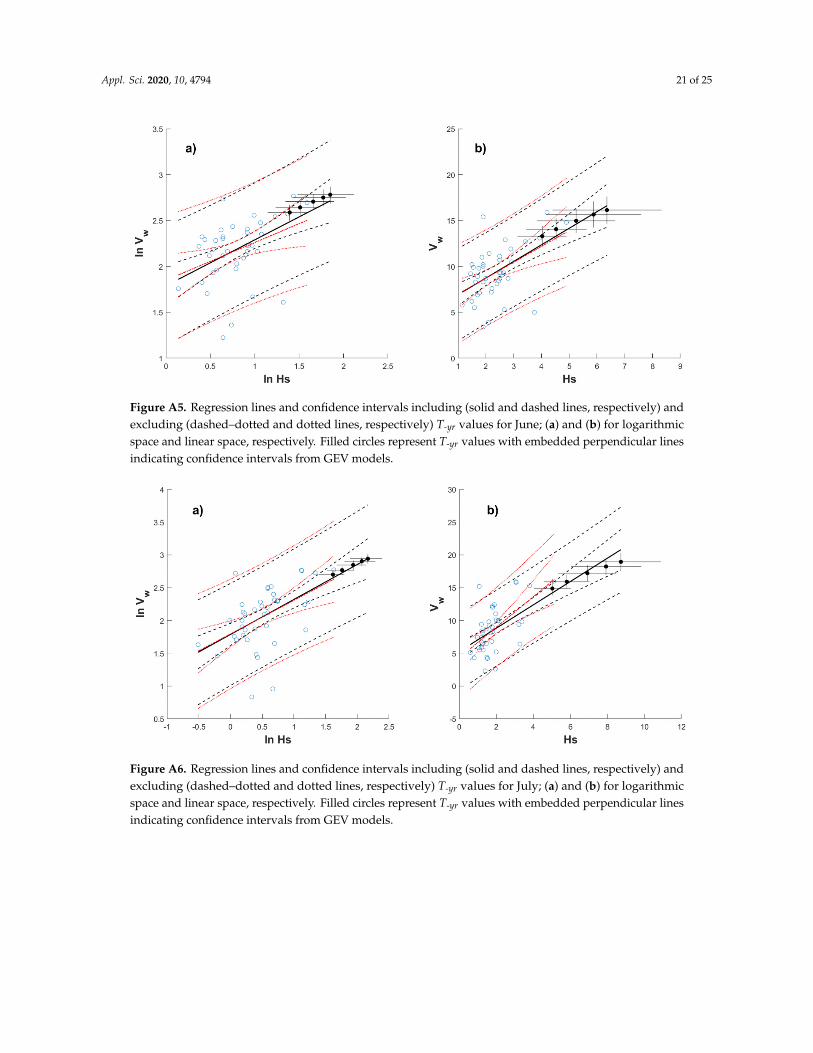
Appl. Sci. 2020, 10, 4794 21 of 25
A4l. Sci. 2020, 10, x FOR P9R REVIEW 21 of 25
Figure A4. Regression lines and confidence intervals including (solid and dashed lines, respectively) and excluding (dashed–dotted and dotted lines, respectively) T-yr values for May; (a) and (b) for logarithmic space and linear space, respectively. Filled circles represent T-yr values with embedded perpendicular lines indicating confidence intervals from GEV models.
Figure A5. Regression lines and confidence intervals including (solid and dashed lines, respectively) and excluding (dashed–dotted and dotted lines, respectively) T-yr values for June; (a) and (b) for logarithmic space and linear space, respectively. Filled circles represent T-yr values with embedded perpendicular lines indicating confidence intervals from GEV models.
Figure A5. Regression lines and confidence intervals including (solid and dashed lines, respectively) andexcluding (dashed–dotted and dotted lines, respectively) T-yr values for June; (a) and (b) for logarithmicspace and linear space, respectively. Filled circles represent T-yr values with embedded perpendicular linesindicating confidence intervals from GEV models.
A4l. Sci. 2020, 10, x FOR P9R REVIEW 22 of 25
Figure A6. Regression lines and confidence intervals including (solid and dashed lines, respectively) and excluding (dashed–dotted and dotted lines, respectively) T-yr values for July; (a) and (b) for logarithmic space and linear space, respectively. Filled circles represent T-yr values with embedded perpendicular lines indicating confidence intervals from GEV models.
Figure A7. Regression lines and confidence intervals including (solid and dashed lines, respectively) and excluding (dashed–dotted and dotted lines, respectively) T-yr values for September; (a) and (b) for logarithmic space and linear space, respectively. Filled circles represent T-yr values with embedded perpendicular lines indicating confidence intervals from GEV models.
Figure A6. Regression lines and confidence intervals including (solid and dashed lines, respectively) andexcluding (dashed–dotted and dotted lines, respectively) T-yr values for July; (a) and (b) for logarithmicspace and linear space, respectively. Filled circles represent T-yr values with embedded perpendicular linesindicating confidence intervals from GEV models.

Appl. Sci. 2020, 10, 4794 22 of 25
A4l. Sci. 2020, 10, x FOR P9R REVIEW 22 of 25
Figure A6. Regression lines and confidence intervals including (solid and dashed lines, respectively) and excluding (dashed–dotted and dotted lines, respectively) T-yr values for July; (a) and (b) for logarithmic space and linear space, respectively. Filled circles represent T-yr values with embedded perpendicular lines indicating confidence intervals from GEV models.
Figure A7. Regression lines and confidence intervals including (solid and dashed lines, respectively) and excluding (dashed–dotted and dotted lines, respectively) T-yr values for September; (a) and (b) for logarithmic space and linear space, respectively. Filled circles represent T-yr values with embedded perpendicular lines indicating confidence intervals from GEV models.
Figure A7. Regression lines and confidence intervals including (solid and dashed lines, respectively)and excluding (dashed–dotted and dotted lines, respectively) T-yr values for September; (a) and (b) forlogarithmic space and linear space, respectively. Filled circles represent T-yr values with embeddedperpendicular lines indicating confidence intervals from GEV models.
A4l. Sci. 2020, 10, x FOR P9R REVIEW 23 of 25
Figure A8. Regression lines and confidence intervals including (solid and dashed lines, respectively) and excluding (dashed–dotted and dotted lines, respectively) T-yr values for November; (a) and (b) for logarithmic space and linear space, respectively. Filled circles represent T-yr values with embedded perpendicular lines indicating confidence intervals from GEV models.
Figure A9. Regression lines and confidence intervals including (solid and dashed lines, respectively) and excluding (dashed–dotted and dotted lines, respectively) T-yr values for December; (a) and (b) for logarithmic space and linear space, respectively. Filled circles represent T-yr values with embedded perpendicular lines indicating confidence intervals from GEV models.
Appendix C
Table A3. Mean values of residuals for each month and regression scheme.
Month Log. Space Lin. Space January 7.8 × 10⁻¹⁷ –4.5 × 10⁻¹⁶
February 3.4 × 10⁻¹⁶ 1.9 × 10⁻¹⁵ March –5.1 × 10⁻¹⁶ 1.4 × 10⁻¹⁵ April 1.8 × 10⁻¹⁷ 1.4 × 10⁻¹⁵ May –3.3 × 10⁻¹⁶ 9.1 × 10⁻¹⁷ June 4.8 × 10⁻¹⁷ –1.3 × 10⁻¹⁵
Figure A8. Regression lines and confidence intervals including (solid and dashed lines, respectively)and excluding (dashed–dotted and dotted lines, respectively) T-yr values for November; (a) and (b) forlogarithmic space and linear space, respectively. Filled circles represent T-yr values with embeddedperpendicular lines indicating confidence intervals from GEV models.

Appl. Sci. 2020, 10, 4794 23 of 25
A4l. Sci. 2020, 10, x FOR P9R REVIEW 23 of 25
Figure A8. Regression lines and confidence intervals including (solid and dashed lines, respectively) and excluding (dashed–dotted and dotted lines, respectively) T-yr values for November; (a) and (b) for logarithmic space and linear space, respectively. Filled circles represent T-yr values with embedded perpendicular lines indicating confidence intervals from GEV models.
Figure A9. Regression lines and confidence intervals including (solid and dashed lines, respectively) and excluding (dashed–dotted and dotted lines, respectively) T-yr values for December; (a) and (b) for logarithmic space and linear space, respectively. Filled circles represent T-yr values with embedded perpendicular lines indicating confidence intervals from GEV models.
Appendix C
Table A3. Mean values of residuals for each month and regression scheme.
Month Log. Space Lin. Space January 7.8 × 10⁻¹⁷ –4.5 × 10⁻¹⁶
February 3.4 × 10⁻¹⁶ 1.9 × 10⁻¹⁵ March –5.1 × 10⁻¹⁶ 1.4 × 10⁻¹⁵ April 1.8 × 10⁻¹⁷ 1.4 × 10⁻¹⁵ May –3.3 × 10⁻¹⁶ 9.1 × 10⁻¹⁷ June 4.8 × 10⁻¹⁷ –1.3 × 10⁻¹⁵
Figure A9. Regression lines and confidence intervals including (solid and dashed lines, respectively)and excluding (dashed–dotted and dotted lines, respectively) T-yr values for December; (a) and (b) forlogarithmic space and linear space, respectively. Filled circles represent T-yr values with embeddedperpendicular lines indicating confidence intervals from GEV models.
Appendix C
Table A3. Mean values of residuals for each month and regression scheme.
Month Log. Space Lin. Space
January 7.8 × 10⁻¹⁷ –4.5 × 10⁻¹⁶
February 3.4 × 10⁻¹⁶ 1.9 × 10⁻¹⁵
March –5.1 × 10⁻¹⁶ 1.4 × 10⁻¹⁵
April 1.8 × 10⁻¹⁷ 1.4 × 10⁻¹⁵
May –3.3 × 10⁻¹⁶ 9.1 × 10⁻¹⁷
June 4.8 × 10⁻¹⁷ –1.3 × 10⁻¹⁵
July 1.4 × 10⁻¹⁶ 8.9 × 10⁻¹⁶
August 4.3 × 10⁻¹⁶ –3.2 × 10⁻¹⁵
September –4.4 × 10⁻¹⁶ 9.5 × 10⁻¹⁶
October 0.0 8.9 × 10⁻¹⁶
November 9.9 × 10⁻¹⁷ –1.4 × 10⁻¹⁵
December –5.6 × 10⁻¹⁷ –2.4 × 10⁻¹⁶
References
1. Castillo, E.; Hadi, A.S.; Balakrishnan, N.; Sarabia, J.M. Extreme Value and Related Models with Applications inEngineering and Science; Wiley: Hoboken, NJ, USA, 2004; Volume 4, pp. 1–362.
2. Hong, H.P. Estimate of extreme wind and wave loading and safety level of offshore structures. In Proceedingsof the Risk Analysis: Proceedings of a Symposium, Ann Arbor, MI, USA, 11–12 August 1994; University ofMichigan: Ann Arbor, MI, USA, 1994; Volume 4, pp. 107–117.
3. Nessim, M.A.; Hong, H.P.; Swail, V.R.; Henderson, C.A. Design criteria for offshore structures under combinedwind and wave loading. J. Offshore Mech. Arct. Eng. 1995, 117, 1–11. [CrossRef]
4. Shao, Z.; Liang, B.; Li, H.; Lee, D. Study of sampling methods for assessment of extreme significant wave heightsin the South China Sea. Ocean Eng. 2018, 168, 173. [CrossRef]

Appl. Sci. 2020, 10, 4794 24 of 25
5. Shao, Z.; Liang, B.; Li, H.; Wu, G.; Wu, Z. Blended wind fields for wave modeling of tropical cyclones in the theSouth China Sea and East China Sea. Appl. Ocean Res. 2018, 71, 20. [CrossRef]
6. Ludeno, G.; Serafino, F. Estimation of the Significant Wave Height from Marine Radar Images without ExternalReference. J. Mar. Sci. Eng. 2019, 7, 432. [CrossRef]
7. Chen, S.-T.; Wang, Y.-W. Improving Coastal Ocean Wave Height Forecasting during Typhoons by using LocalMeteorological and Neighboring Wave Data in Support Vector Regression Models. J. Mar. Sci. Eng. 2020, 8, 149.[CrossRef]
8. Gao, H.; Shao, Z.; Wu, G.; Li, P. Study of Directional Declustering for Estimating Extreme Wave Heights in theYellow Sea. J. Mar. Sci. Eng. 2020, 8, 236. [CrossRef]
9. Katalinic, M.; Parunov, J. Uncertainties of Estimating Extreme Significant Wave Height for EngineeringApplications Depending on the Approach and Fitting Technique—Adriatic Sea Case Study. J. Mar. Sci. Eng. 2020,8, 259. [CrossRef]
10. Cavaleri, L.; Barbariol, F.; Benetazzo, A. Wind–Wave Modeling: Where We Are, Where to Go. J. Mar. Sci. Eng.2020, 8, 260. [CrossRef]
11. Weisse, R.; Gaslikova, L.; Geyer, B.; Groll, N.; Meyer, E. Coastdat—Model data for science and industry.Kuste Westholsteinische Verl. Boyens Co. 2014, 81, 5–18.
12. Weisse, R.; Groll, N. A multi-decadal wind-wave hindcast for the North Sea 1949–2014: CoastDat2. Earth Syst.Sci. Data 2017, 9, 955.
13. Monish, N.T.; Rehana, S. Suitability of distributions for standard precipitation and evapotranspiration index overmeteorologically homogeneous zones of India. J. Earth Syst. Sci. 2020, 129, 25. [CrossRef]
14. Schardong, A.; Simonovic, S.P.; Gaur, A.; Sandink, D. Web-Based Tool for the Development of Intensity DurationFrequency Curves under Changing Climate at Gauged and Ungauged Locations. Water 2020, 12, 1243. [CrossRef]
15. Prakash, A.; Panchang, V.; Ding, Y.; Ntaimo, L. Sign Constrained Bayesian Inference for Nonstationary Models ofExtreme Events. J. Waterw. Port Coast. Ocean Eng. ASCE 2020, 146, 04020029. [CrossRef]
16. Kim, H.-J.; Suh, S.-W. Improved Hypothetical Typhoon Generation Technique for Storm Surge FrequencyAnalyses on the Southwest Korean Coast. J. Coast. Res. 2018, 85, 516. [CrossRef]
17. Weinan, H.; Shanshan, T.; Qiang, B.; Sheng, D. Bivariate Distribution Modelling for Wave Height and Period inJiaozhou Bay. In Proceedings of the ASME 2018 37th International Conference on Ocean, Offshore and ArcticEngineering 2018, Volume 11B: Honoring Symposium for Professor Carlos Guedes Soares on Marine Technologyand Ocean Engineering, Madrid, Spain, 17–22 June 2018. V11BT12A054. [CrossRef]
18. Sartini, L.; Besio, G.; Cassola, F. Spatio-temporal modelling of extreme wave heights in the Mediterranean Sea.Ocean Model. 2017, 117, 52. [CrossRef]
19. Muraleedharan, G.; Lucas, C.; Guedes Soares, C. Regression quantile models for estimating trends in extremesignificant wave heights. Ocean Eng. 2016, 118, 204. [CrossRef]
20. Ross, E.; Astrup, O.C.; Bitner-Gregersen, E.; Bunn, N.; Feld, G.; Gouldby, B.; Liu, Y.; Randell, D.; Vanem, E.;Jonathan, P. On environmental contours for marine and coastal design. Ocean Eng. 2020, 195, 1. [CrossRef]
21. Vanem, E. A simple approach to account for seasonality in the description of extreme ocean environments.Mar. Syst. Ocean Technol. 2018, 13, 63. [CrossRef]
22. Randell, D.; Feld, G.; Ewans, K.; Jonathan, P. Distributions of return values for the ocean wave characteristics inthe South China Sea using directional-seasonal extreme value analysis. Environmetrics 2015, 26, 442. [CrossRef]
23. Randell, D.; Turnbull, K.; Ewans, K.; Jonathan, P. Bayesian inference for nonstationary marginal extremes.Environmetrics 2016, 27, 439. [CrossRef]
24. Ross, E.; Randell, D.; Ewans, K.; Feld, G.; Jonathan, P. Efficient estimation of return value distributions fromnon-stationary marginal extreme value models using Bayesian inference. Ocean Eng. 2017, 142, 315. [CrossRef]
25. Anokhin, V.; Randell, D.; Ross, E.; Jonathan, P. Spatial and seasonal variability of metocean design criteria inthe southern south China Sea from covariate extreme value analysis. In Proceedings of the ASME 2019 38thInternational Conference on Ocean, Offshore and Artic Engineering, OMAE, Glasgow, Scotland, UK, 9–14 June2019; Volume 1.

Appl. Sci. 2020, 10, 4794 25 of 25
26. Bitner-Gregersen, E.M. Comparison of wind and wave climate in open sea and coastal waters. Ocean Eng. 2018,170, 199. [CrossRef]
27. National Data Buoy Center (NDBC). Available online: www.ndbc.noaa.gov (accessed on 30 June 2020).28. Calderón-Vega, F.; Vázquez-Hernández, A.O.; García-Soto, A.D. Analysis of extreme waves with seasonal
variation in the Gulf of Mexico using a time-dependent GEV model. Ocean Eng. 2013, 73, 68–82. [CrossRef]29. Coles, S.G. An Introduction to Statistical Modelling of Extreme Values, 1st ed.; Springer: London, UK, 2001; Volume 4,
pp. 1–208.30. Calderón Vega, F. Caracterización del Régimen Extremal del Oleaje en el Golfo de México Considerando la
Variación Estacional. Master’s Thesis, Universidad de Cantabria, Santander, Spain, 2009. (In Spanish)31. Bitner-Gregersen, E.M.; Gramstad, O. Potential Changes in the Joint Probabilistic Description of the North
Atlantic Wave Climate. In Proceedings of the ASME 2018 37th International Conference on Ocean, Offshore andArctic Engineering, Volume 11B: Honoring Symposium for Professor Carlos Guedes Soares on Marine Technologyand Ocean Engineering, Madrid, Spain, 17–22 June 2018. V11BT12A056. [CrossRef]
32. Hong, H.P.; Zimmerman, T.J.; Bach, L. Probabilistic basis of resistance factors for use in oriented strand board.In Proceedings of the 1st Structural Specialty Conference, Canadian Society of Civil Engineering, Edmonton, AB,Canada, 29 May–1 June 1996; pp. 1223–1235.
33. Jordaan, I. Decisions under Uncertainty: Probabilistic Analysis for Engineering Decisions, 1st ed.; Cambridge UniversityPress: Cambridge, UK, 2005; pp. 1–672.
34. Kottegoda, N.T.; Rosso, R. Applied Statistics for Civil and Environmental Engineers, 2nd ed.;Blackwell Publishing-Wiley: Oxford, UK, 2008; pp. 1–718.
35. Faber, M.H. Statistics and Probability Theory: In Pursuit of Engineering Decision Support, 2nd ed.; Springer: Dordrecht,The Netherlands; Heidelberg, Germany; London, UK; New York, NY, USA, 2012; pp. 1–190.
© 2020 by the authors. Licensee MDPI, Basel, Switzerland. This article is an open access articledistributed under the terms and conditions of the Creative Commons Attribution (CC BY)license (http://creativecommons.org/licenses/by/4.0/).

82
Paper B
Revisiting Two Simulation‐Based Reliability Approaches for Coastal and Structural Engineering Applications. Adrián‐David García‐Soto, Felícitas Calderón‐Vega, César Mösso, Jesús‐Gerardo Valdés‐Vázquez and Alejandro Hernández‐Martínez Applied Sciences. Appl. Sci. 2020, 10, 8176; doi:10.3390/app10228176.

Appl. Sci. 2020, 10, 8176; doi:10.3390/app10228176 www.mdpi.com/journal/applsci
Article
Revisiting Two Simulation‐Based Reliability
Approaches for Coastal and Structural
Engineering Applications
Adrián‐David García‐Soto 1,*, Felícitas Calderón‐Vega 1,2, César Mösso 2,3,
Jesús‐Gerardo Valdés‐Vázquez 1 and Alejandro Hernández‐Martínez 1
1 Department of Civil Engineering, Universidad de Guanajuato, Juárez 77, Zona Centro,
Guanajuato 36000, Gto., Mexico; [email protected] (F.C.‐V.); [email protected] (J.‐G.V.‐V.);
[email protected] (A.H.‐M.) 2 Laboratori d’Enginyeria Marítima, Universitat Politècnica de Catalunya, Jordi Girona 1‐3, Mòdul D1,
Campus Nord, 08034 Barcelona, Spain; [email protected] 3 Centre Internacional d’Investigació dels Recursos Costaners, Jordi Girona 1‐3, Mòdul D1, Campus Nord,
08034 Barcelona, Spain
* Correspondence: [email protected]; Tel.: +52‐473‐1020‐100 (ext. 2235)
Received: 17 October 2020; Accepted: 17 November 2020; Published: 18 November 2020
Featured Application: Normality polynomials can be used to compute reliabilities for coastal and
structural engineering applications, including the assessment of uncertainty in the estimated
reliability index. Additionally, multi‐linear regression can be applied to the simulated results to
determine design points and sensitivity factors. These applications can be potentially extended
to different engineering (or other) fields and to system reliability (e.g., for reinforced concrete
frame buildings).
Abstract: The normality polynomial and multi‐linear regression approaches are revisited for
estimating the reliability index, its precision, and other reliability‐related values for coastal and
structural engineering applications. In previous studies, neither the error in the reliability estimation
is mathematically defined nor the adequacy of varying the tolerance is investigated. This is
addressed in the present study. First, sets of given numbers of Monte Carlo simulations are obtained
for three limit state functions and probabilities of failure are computed. Then, the normality
polynomial approach is applied to each set and mean errors in estimating the reliability index are
obtained, together with its associated uncertainty; this is defined mathematically. The data is also
used to derive design points and sensitivity factors by multi‐linear regression analysis for given
tolerances. Results indicate that power laws define the mean error of the reliability index and its
standard deviation as a function of the number of simulations for the normality polynomial
approach. Results also indicate that the multi‐linear regression approach accurately predicts
reliability‐related values if enough simulations are performed for a given tolerance. It is concluded
that the revisited approaches are a valuable option to compute reliability‐associated values with
reduced simulations, by accepting a quantitative precision level.
Keywords: reliability index error; power law; normality polynomial; multi‐linear regression;
sensitivity factors; coastal engineering; structural engineering

Appl. Sci. 2020, 10, 8176 2 of 21
1. Introduction
Simulations are often used to estimate the probability of failure of structural elements and
systems because they are a very versatile option which is not restricted by complex and implicit limit
state functions (LSF), the use of sophisticated methods (e.g., finite element method), and/or highly
non‐linear structural behavior. However, millions of crude Monte Carlo simulations (MCS) could be
required to adequately estimate structural probabilities of failure, which may not be feasible; also,
the results could differ from a set of simulations to another. To cope with this issue, modified versions
of the crude simulation approach, surrogate modeling, subset simulation, and other techniques have
emerged and been used in the last decades not only for structural engineering but also in other fields.
To mention only a few studies which employ some of these techniques, optimization using surrogate
modeling, reliability analysis of deteriorating structural systems and the reliability assessment of a
structure affected by chloride attack are reported in the studies by [1–3], respectively. Importance
sampling has also been used to estimate the system reliability of deteriorating pipelines [4]. Other
kind of approaches are also reported in the literature to compute reliabilities [5]. The different
reliability methods can be applied not only to different fields in structural and geotechnical
engineering, as for the case of sudden column removal in reinforced concrete buildings and rockfall
protection structures [6–8], but also to many other research and engineering fields, for instance to
artic oil and gas facilities [9] and to coastal engineering applications [10]. This last case is used in the
present study to show the applicability of two revisited methods to obtain the reliability of coastal
structures.
Other simulation‐based reliability methods have not been given so much attention. In this study
a couple of these alternatives are revisited to inspect their feasibility and adequacy to estimate
reliability indices. One of them employs polynomial transformations of a nonnormal variable to a
normal one by fitting simulated data with fractile constraints and can be referred to as normality
polynomial approach [11]. The second approach was developed to derive the design point and
sensitivity factors (in the FORM, first order reliability method, perspective) from simulated data [12]
and it is referred to as the multi‐linear regression approach in this study. A similar approach to the
normality polynomial method was previously developed by Hong and Lind [13] and named normal
polynomial approach (note that the names are slightly different); unlike the normality polynomial
approach, the normal polynomial approach has been paid much more attention (judging by number
of citations), even very recently (e.g., [14]). Both methods are based on the fact [15,16] that a fractile
of a random variable can be expressed as polynomial of a fractile of a standard normal variable
(normal polynomial), and that a fractile of a standard normal variable can be expressed as a
polynomial of a fractile of a random variable (normality polynomial). Although the normal
polynomial approach [13] is not considered in the present study (we prefer to focus in the less
explored alternative), the findings here could be extended to do so.
To inspect the adequacy of the normality polynomial approach and the multi‐linear regression
approach (the methods revisited in the present study), three LSFs are considered. One is based on a
very simple classical case; other one is based on a structural application from a previous study and
the last one is related to the reliability of a coastal structure. Extensive simulations are performed to
estimate the error level by using the normality polynomial approach and its associated uncertainty;
neither of these was thoroughly carried out in previous studies, nor the application to coastal
engineering. The design point and sensitivity factors (also the reliability index) obtained from
simulated data are compared with those obtained from FORM; they are derived from a multi‐linear
regression of the simulated data. It is worth to mention that these methods, and others developed in
the 1990s, used to state that a large number of simulations were not feasible; nevertheless, the
computer power has increased substantially in the last decades, and the limitations of those days may
not be as restrictive as before and thus the applicability could be currently extended. Furthermore,
the commercial software available nowadays for engineering applications normally includes
amenable built‐in functions for linear and multi‐linear regression analysis which simplifies the
programming.

Appl. Sci. 2020, 10, 8176 3 of 21
The main objective of this study is to define the error statistics in the reliability index by using
normality polynomials and to reassess the feasibility and adequacy of this method and the multi‐
linear regression approach for estimating the reliability of structural and coastal engineering systems
including the determination of sensitivity factors.
This study is of significance to the coastal and structural engineering fields because the number
of simulations required to compute reliabilities can be reduced by accepting defined error levels
when using normality polynomials, which was not established in previous studies. This is possible
because the error in the estimation of the reliability index is mathematically defined as a function of
the number of simulations for the cases investigated. Additionally, other contribution is the use of
multi‐linear regression applied to simulated results as a mean to determine sensitivity factors, design
points and the probability of failure; not only a slightly modified (improved) version of the multi‐
linear regression approach but also the number of simulations and tolerances required to achieve
adequate results are provided for guidance.
2. Methods Revisited
2.1. Normality Polynomial
In this section the normality polynomial proposed in [11] is described. The mathematical form
is given by
𝑧 𝑎 𝑦 (1)
where zp denotes p‐fractile of a standard normal variable Z with probability density function (PDF),
Φ(z), and cumulative distribution function (CDF), Φ(z); yp denotes p‐fractile of a random variable Y
with PDF, fY(y), and CDF, FY(y); aj, j = 1, 2, …, r, are the coefficients of a rth‐order polynomial
determined by fractile fitting. The fractile fitting is based on considering the following fractile
constraints from a set of independent random observations of Y (i.e., y1, y2, … yi, … yn) arranged in
ascending order
𝑦 ,𝐹 𝑦 𝑦 ,𝑖
𝑛 1, 𝑖 1, 2, . . . ,𝑛 (2)
These fractile constraints can be mapped into a normal space by using
𝑧 Φ 𝐹 𝑦 , 𝑖 1, 2, . . . ,𝑛 (3)
where Φ−1(•) denotes the inverse of the standardized normal distribution function. The rth‐order
polynomial (Equation (1)) with r + 1 < n is used to model the distribution of the transformed random
variable Y. By considering the constraints in Equation (2), the coefficients aj in Equation (1) can be
determined using the least square method by minimizing the error εfit given by
𝜀 𝑧 𝑎 𝑦 (4)
where m is the number of constraints. The probability P (Y ≤ y0) is given by the CDF, i.e., F(y0), and
can be computed with
𝐹 𝑦 Φ 𝑧 (5)
where zp is obtained by substituting y0 instead of yp in Equation (1). If Y is the resulting random
variable of the LSF, the probability of failure, pf, is
𝑝 𝐹 0 Φ 𝑎 (6)
and the reliability index is [17]
𝛽 Φ 𝑝 (7)

Appl. Sci. 2020, 10, 8176 4 of 21
From Equation (7), it can be inferred that the reliability index can be readily obtained once the
coefficients aj are determined (i.e., β = −a0). This is so, because a0 has a similar meaning to the so‐called
generalized reliability index [11]. It is noted that the roots of the polynomial are not required [11]
(unlike in the method in [13]). In the applications shown later, a third‐order normality polynomial is
used [11].
It is pointed out that although the mathematical background of the normality polynomials is not
thoroughly described here, it is based on sound grounds [11], like the advance theory of statistics
[15,16] and the fact that fractile constraints hold by a combinatorial argument [18,19].
Before going to the applications, the second revisited approach in this study is described in the
following section.
2.2. Design Point and Sensitivity Factors from Simulations
The obtaining of the design point and sensitivity factors (from the FORM standpoint) based on
a previous study [12] is described herein. The basic idea is that simulated data close to the limit state
surface (within a prescribed tolerance, e) can be retrieved, as well as their associated sampled values
for each or the random variables given by the LSF (input values combinations considered as a point
in the hyperspace), and a multi‐linear regression is performed to approximate the linearized limit
state surface at the design point. Before the multi‐linear regression is performed to fit the hyperplane,
the considered points are mapped into a standard normal space. Such hyperplane is an
approximation of the LSF, g, and is used to assess the design point and sensitivity factors. The
mathematical formulation is given below.
A set of n independent random variables is denoted by X = (x1, x2, …, xn). Xj defines the j‐th
randomly generated value of X. For a given number of crude Monte Carlo simulations, nsim, Xjs which
satisfy the criterion below (slightly changed from the original formulation in [12]) are selected
|0 g 𝑿 | 𝑒 (8)
where Xk in the LSF is included to emphasize that it is a function of a set of random variables. Hong
and Nessim [12] used e = 0.05 (i.e., 5%) in their study (instead of el in Equation (8) and defined below).
However, it was noticed that this value could be inadequate depending on the units and magnitude
of the considered random variables. Therefore, the distance between zero and the smallest simulated
value of g in absolute terms (llow) is used to set the tolerance as the fraction given by llow multiplied by
e (i.e., el = e × llow is used instead of e in Equation (8)). The selected values of Xk based on the described
criterion are then mapped into a standard normal space [17] using
𝒁 𝑧 , 𝑧 , … , 𝑧 Φ 𝐹 𝑥 ,Φ 𝐹 𝑥 , … ,Φ 𝐹 𝑥 (9)
where Z is the image of X in standard normal space, Φ is the normal standard CDF and Fi, I = 1, 2, …,
n, are the CDFs of the random variables xi. In the standard normal space, a linear function is fitted to
the set of selected points using multi‐linear regression. Such linear function is given by
𝑏 𝑧 𝑐 0 (10)
where bi and c are constants to be determined in the multi‐linear regression analysis. The resulting
linear regression equation is to be used in the same sense as the FORM [17] to estimate the design
point and sensitivity factors. The latter are denoted by αi, i = 1, 2, …, n, and given by the gradient
vector of Equation (10) as indicated below
𝛼 𝑏∑ 𝑏
(11)
Note that the reliability index can also be estimated as the smallest distance between the linear
surface and the origin as
𝛽 𝑐∑ 𝑏
(12)
As regards the design point (in the normal space) it is given by

Appl. Sci. 2020, 10, 8176 5 of 21
𝑧 𝛼 𝛽 (13)
The design point in the original space can now be determined with the inverse transformation
of zid, as
𝑥 𝐹 Φ 𝑧 (14)
The subscript i in Equations (11)–(14) is associated to the random variable xi. The inverse
transformation in Equation (14) is dependent on the PDF of xid and, in the case of the Longuet‐Higgins
distribution [20] used for the coastal engineering example, the inverse transformations of zid requires
of a numerical approach to be determined.
The formulation in this section, and the one in the previous section, are to be applied to three
case studies in the following section to evaluate their adequacy for structural and coastal engineering,
and to assess their deviation with respect to the exact reliability index.
3. Applications and Results
3.1. A Classical Limit State Funtion
The two approaches described in the previous section are applied here to the simplest classical
LSF
𝑔 𝑅 𝐿 (15)
where R and L can be considered, in a broad sense, as random variables for the capacity and demand
of a system element. For the sake of simplicity and illustration purposes, units are skipped and both
random variables are assumed independent and characterized with lognormal distributions, with
mean values and standard deviations mR = 10, mL = 5.6, σR = 1, and σL = 0.75 for the capacity and
demand, respectively. These values are arbitrary, except by the fact that they lead to a reliability index
equal to practically 3.5, which is a common reference for code calibration and that can be computed
with the following expression [21,22]
𝛽𝑙𝑛 𝑚 1
2 ln 1 𝜐 𝑙𝑛 𝑚 12 ln 1 𝜐
ln 1 𝜐 ln 1 𝜐
ln𝑚 ln𝑚
𝜐 𝜐 (16)
where νR and νL are the coefficients of variation of R and L, respectively. This reliability index is shown
in Figure 1a (dashed line), as a reference to inspect how close are the βs obtained by crude Monte
Carlo simulations as a function of the number of simulations (shown in logarithmic scale in the
horizontal axis from 2 × 101 to 2 × 10⁷) to the exact value. The reliability index for Equation (15) using
Monte Carlo simulations (dashed‐dotted line in Figure 1a) is obtained by plugging into Equation (7)
the following probability of failure
𝑝𝑛
𝑛 (17)
which is simply the ratio of number of failures, nfail, to the total number of simulations. The latter (i.e.,
nsim) is also the number of fractile constraints when the reliability index is computed with the
normality polynomial approach, also depicted in Figure 1a (solid line).
Additional runs are shown in Figure 1b–d, which indicate that the results are different and
dependent on the generated random numbers of each run, but they stabilize if enough simulations
are performed or enough fractile constraints are used. Other observations from Figure 1 include that
β cannot always be computed with the Monte Carlo simulations (MCS) (not a single failure is
obtained), while the opposite occurs when using normality polynomials, although significant
deviations are observed for a limited number of simulations, that the fitted normality polynomials
tends to deviate less from the exact reliability index for fewer nsim, and that such error in the precision
may not be large for a relative small nsim, (e.g., 1 × 10³).

Appl. Sci. 2020, 10, 8176 6 of 21
Figure 1. Reliability index as a function of the number of simulations. (a), (b), (c) and (d) are different
runs for the MCS.
To quantitatively inspect these deviations, βRE is to be used as benchmark to assess the exactness
of the used methods (i.e., normality polynomials and MCS) in terms of the relative percentual error
given by
𝜀𝛽 𝛽
𝛽100 (18)
where βbench denotes the reliability index considered as benchmark and βoth is the reliability index
computed with any other method. A total of 1000 runs are performed for each nsim, and ε is computed
for each of the runs. Then, the mean values of the error and their uncertainties (the unbiased standard
deviation) are computed and plotted for the whole range of nsim in Figure 2 (solid lines and dashed
lines for normality polynomial and MCS mean errors, respectively), where the mean errors ± one
standard deviation are also depicted in grey lines.
Figure 2 shows that is not always possible to compute the statistics for the MCS; this happens
when not a single failure is reported in one or more of the 1000 runs for a given nsim (at least 5 × 10⁴
are necessary). This is not a problem when using the fitted polynomials. Additionally, the MCS
approach always tend to larger mean errors and standard deviations for a decreasing number of
simulations. This makes the normality polynomial approach more adequate for estimating the
reliability indices; however, for few simulations the errors are too large. Nevertheless, the designer
could decide which precision level (quantitatively) is willing to accept using information like the one
in Figure 2 as an aid (and reduce the number of required simulations as a function of such an accepted
error).

Appl. Sci. 2020, 10, 8176 7 of 21
Figure 2. Deviations from the exact reliability index as percentage error.
If desired, the curves in Figure 2 could be casted as a mathematical expression. For instance, the
following power equations fit very well the mean (με) and standard deviation (σε) of the error in
Figure 2 (by fitting from 2.5 × 10² simulations and over)
𝜇 257.2 𝑛 . (19)
𝜎 157.3 𝑛 . (20)
If the power in Equations (19) and (20) is assumed as −0.5 in both expressions, the coefficient of
variation of the error is νε ≈ 150/250 ≈ 0.6, i.e., it is constant and roughly independent of the number
of simulations; the actual νε obtained from the 1000 runs does exhibit such a roughly constant
behavior for this case, except that it is ≈0.7 (difference related to the actual different powers in
Equations (19) and (20)). Power equations like Equations (19) and (20) can be linearized by taking
logarithms on both sides. Therefore, if the involved variables are transformed into the logarithmic
space, a linear fitting can be performed. In this study, we simply used a built‐in function in the
commercial software for the fitting.
Coefficients for the fitted normality polynomial in Figure 1a are shown in Table 1 (upper set of
values) for selected values of nsim. The computing of these coefficients is based on minimizing the
error in Equation (4) and was implemented in the coded program by using a built‐in function of the
programming language employed (MATLAB). As mentioned before, the coefficients a0 can be linked
to the generalized reliability index. Coefficients for results in Figure 1b–d (or those associated to
Figure 2) were computed but not shown for brevity.
As regards the reliability index, design point and sensitivity factors derived from the simulations
(i.e., those obtained with Equations (11), (12), and (14)), they are compared with those obtained by
applying the FORM to Equation (15). They are summarized in Table 2 for selected values of nsim.
Results listed in Table 2 indicate that when the points obtained by applying the criterion in
Equation (8) were enough to successfully perform a multi‐linear regression (also with a built‐in
function, as in the case of the normality polynomial fitting), β did not deviate from the exact value,
but marginally, just like the reliability index obtained with FORM. However, a relatively large nsim
was required, usually at least 1 × 10⁵ simulations (by inspecting all the 1000 × nsim cases used to derived
Figure 2); this depends on each run (implicitly the generated random numbers in each simulation),
and sometimes less than 1 × 10⁵ simulations are required. For the considered runs, 2 × 10⁵ simulations
seem to guarantee the obtaining of the values reported in Table 2. In any case, when the muti‐linear
regression is successfully performed, the results are quite adequate and invariant for increasing
number of simulations; this is also the case for the coefficients of the regression (i.e., they remain
independent of nsim), which are c = 0.5837, b1 = 0.0998, and b2 = −0.1333.

Appl. Sci. 2020, 10, 8176 8 of 21
Table 1. Coefficients of the fitted normality polynomials.
Classic LSF, Equation (15)
nsim a0 a1 a2 a3 a4
1 × 10³ −3.1193 3.9078 3.6571 −1.9371 ‐‐‐‐
1 × 10⁴ −3.3195 4.9672 1.8106 −0.9905 ‐‐‐‐
1 × 10⁵ −3.4813 5.8709 0.2415 −0.1324 ‐‐‐‐
Structural LSF, Equation (21) rV/D = 0.4
nsim a0 a1 a2 a3 a4
1 × 10³ −3.0950 6.3170 × 10−07 3.8257 × 10⁻¹⁴ −3.2619 × 10⁻²¹ ‐‐‐‐
1 × 10⁴ −3.2923 7.3372 × 10−07 2.1457 × 10⁻¹⁴ −2.3097 × 10⁻²¹ ‐‐‐‐
1 × 10⁵ −3.3341 7.8972 × 10−07 5.2658 × 10⁻¹⁵ −1.0534 × 10⁻²¹ ‐‐‐‐
Structural LSF, Equation (21) rV/D = 0.4 4th‐order
nsim a0 a1 a2 a3 a4
1 × 10³ −2.8726 1.7464 × 10−07 2.7997 × 10⁻¹³ −5.0461 × 10⁻²⁰ 3.1134 × 10⁻²⁷
1 × 10⁴ −3.2802 6.7401 × 10−07 6.0193 × 10⁻¹⁴ −1.0616 × 10⁻²⁰ 5.7321 × 10⁻²⁸
1 × 10⁵ −3.2799 7.1276 × 10−07 3.6215 × 10⁻¹⁴ −5.7785 × 10⁻²¹ 2.4322 × 10⁻²⁸
Table 2. Design point, β and αi by using multi‐linear regression and first order reliability method
(FORM).
Design Point Sensitivity Factors
nsim β xR xL αR αL
1 × 10⁴ ‐‐‐‐ ‐‐‐‐ ‐‐‐‐ ‐‐‐‐ ‐‐‐‐
5 × 10⁴ ‐‐‐‐ ‐‐‐‐ ‐‐‐‐ ‐‐‐‐ ‐‐‐‐
1 × 10⁵ 3.5055 8.0699 8.0699 −0.5990 0.8007
2 × 10⁵ 3.5055 8.0699 8.0699 −0.5990 0.8007
1 × 10⁶ 3.5055 8.0699 8.0699 −0.5990 0.8007
FORM 3.5055 8.0670 8.0670 −0.5990 0.8007
If the tolerance el in Equation (8) is increased, the minimum number of required simulations can
be decreased. For instance, if e = 0.25 were used (instead of the actual used e = 0.05), 5 × 10⁴ simulations
would be enough for a successful multi‐linear regression. Moreover, the design point, sensitivity
factors and reliability index would be the same as those reported in Table 2. The opposite would
occur if e = 0.005 were used (instead of the actual used e = 0.05), i.e., a much larger number of
simulations would be required to determine the reliability parameters from the regression.
Therefore, this approach based on multi‐linear regression can be quite an adequate alternative
by itself to compute β, conditioned on the feasibility of performing enough simulations, the number
of which can be decreased by using a large e; with the additional advantage that the design point and
sensitivity factors can also be determined.
In the following section a more realistic LSF for a structural application is used to further
investigate the revisited methods.
3.2. Reliability of Reinforced Concrete Beam under Flexure Moment
In this section the approaches described before are applied to a reinforced concrete beam (RCB)
subjected to flexure moment. The example is the same investigated in a previous study [23] but
focused only in one design code [24] and three ratios of the mean live to the mean dead load effect
for the beam. The rectangular beam section information, LSF, and statistics are succinctly reproduced
below. The LSF is
𝑔 𝐵𝐴 𝑓 𝑑 1 0.59𝐴 𝑓𝑓 𝑏𝑑
𝐷 𝑉 (21)
where B is the modeling error, f’c is the concrete compressive strength, As is the reinforcement steel
area, fy is the yielding stress of the reinforcement steel, b is the section width, h is the effective depth,
and D and V are the dead load and live load effect, respectively (flexure moment). The information

Appl. Sci. 2020, 10, 8176 9 of 21
of all the independent variables in Equation (21) is summarized in Table 3. As is assumed
deterministic and equal to 3000 mm2. The PDFs of the random variables in Table 3 are based on
previous literature, which in turn reflects results from experimental projects, field information,
observed phenomena, and even the engineers experience to characterized these variables properly,
since such PDFs have a direct impact in the computed reliabilities, code calibration tasks, and
ultimately in the safety of real structures. More details can be found in [23] and the references therein.
Table 3. Random variables for the limit state functions (LSF) of the reinforced concrete beam (RCB) considered.
Random Variable Mean coeff. of var. PDF
B 1.01 0.06 Normal
f’c (MPa) 31.6 0.145 Normal
fy (MPa) 474 0.05 Lognormal
b (mm) 303 0.04 Normal
d (mm) 990 0.04 Normal
D (kN∙m) * 0.05 Normal
V (kN∙m) * 0.18 Gumbel
* denotes that these values are not determined until a rV/D value is selected and used together with Equation (22).
Mean values of D and V are not defined in Table 3, but they are derived by considering given
mean live load effect (mV) to mean dead load effect (mD) ratios (rV/D = 0.4, 1.0 and 2.0 are used in this
study) and the assumption that the RCB just meets the code requirement; thus, the following
expression is used to determine the mean values.
1.2𝑚 1.6𝑚 𝜙𝐴 𝑚 𝑚 0.59𝐴 𝑚
𝑚 𝑚 (22)
where m denotes the mean values of the variables in the corresponding subscripts, and Φ = 0.9.
Using the previous information, the normality polynomial approach is applied to Equation (21)
and the results are shown in Figures 3 and 4. These figures are analogous to Figures 1 and 2, except
that the reference reliability indices (dashed lines) correspond to the values computed using FORM,
that three cases of the ratio rV/D = mV/mD are depicted (the largest βs correspond to rV/D = 0.4 and the
smallest to rV/D = 2.0, as shown in Figure 3a) and that the error in Figure 4 is shown for rV/D = 0.4 (Figure
4a) and for rV/D = 2.0 (Figure 4b), which is computed by considering in Equation (18) βbench as the
average of the 1000 runs for nsim = 2 × 10⁷ (assumed as the exact value). MCS results are depicted with
dashed‐doted lines. To perform the MCS, mD and mV are defined using Equation (22) and rV/D as
mentioned before. Once they are determined, MCS can then be performed to obtain samples of D and
V (and all other random variables in Table 3) and the probability of failure as per Equation (17) can
be computed. As an example of the simulated bending moments, histograms of D and V are shown
in Appendix A (Figure A1) for 1 × 10⁶ MCS and rV/D = 1.0; it can be observed that the values are
comparable in average (because rV/D = 1.0 is considered), and that histograms for D and V clearly
resemble normal and Gumbel distributions, respectively, which is expected given that these variables
were sampled from such PDFs.
From Figures 3 and 4 similar conclusions to those drawn from Figures 1 and 2 can be extracted.
Some additional observations worth to mention are that nsim = 1 × 10⁴ seems a reasonable number of
simulations for the normality polynomial approach, if a compromise between nsim and error (in terms
of mean and standard deviation) is envisaged, that the fitted polynomials lead to better results than
the FORM for increasing nsim and that larger errors are obtained for smaller rV/D; this latter aspect
could be attributed to a better approximation of the failure surface for larger rV/D, since the first order
approximation to the failure surface by the other method shown in Figure 3 (i.e., the FORM), also
deviates more from the exact value for decreasing rV/D.
By observing Figure 4, it is pointed out once more that error and its uncertainty is less for
normality polynomial when decreasing nsim than for MCS for this case too and, as previously
mentioned, is not always possible to estimate the error for MCS for decreasing number of simulations.

Appl. Sci. 2020, 10, 8176 10 of 21
The error for β obtained with the normality polynomial approach exhibits an asymptotic behavior
towards approximately με = 1% for large nsim. As before, power laws fit adequately the error and its
uncertainty and are defined as
𝜇 𝛿 𝑛 1 (23)
𝜎 𝜅 𝑛 (24)
where δ = 656, 1103, and 1349, γ = 0.7401, 0.8493, and 0.9062, κ = 129.8, 201, and 179.1, τ = 0.4937,
0.5609, and 0.5703 for rV/D = 0.4, 1.0, and 2.0, respectively. In Equation (23) the constant unity is
included to shift the curve upwards to reproduce the asymptotic behavior mentioned; nonetheless,
it could be skipped, and the equations will still fairly adequately describe the mean error. The fitting
for με was performed for the whole range of nsim, while for σε, nsim from 250 and over was employed.
Note that although the range for the fitting could be established based on practical grounds and
fitting improvement, in any case the errors and their uncertainties follow a power law; this is the case
for the three case studies carried out in this study.
Figure 3. Reliability index as a function of the number of simulations for RCB. (a), (b), (c) and (d) are
different runs for the MCS.
It is noteworthy that the normality polynomial approach leads to comparable με and σε for
Figures 2 and 4, considering that the LSF for the RCB is a more complex (non‐linear) function, and
that it has much more random variables and several PDFs.

Appl. Sci. 2020, 10, 8176 11 of 21
Figure 4. Deviations from the exact reliability index as percentage error for RCB; (a) rV/D = 0.4 and (b)
rV/D = 2.0.
The fitted coefficients of the polynomials for Figure 3 (corresponding to rV/D = 0.4) and selected
nsim are listed in Table 1 (middle set of values). If normality polynomials of order higher than 3 are
used, no further accuracy is gained (or even higher inaccuracies could be obtained; [11]). This is
confirmed by carrying out a single case for rV/D = 0.4 using a 4th‐order polynomial, since the results
are comparable to those of the 3rd‐order polynomial case (Table 1, lower set of values). Note that the
order of the coefficients of the normality polynomials for the RCB problem can be very small
(compared to the classical LSF problem and to a coastal engineering application shown later); this
could be due to the units employed, and should not be understood as if the order of the polynomial
could be decreased, whereas obtaining comparable precision, because the use of at least third‐order
normality polynomials was illustrated and found adequate in [11].
To end this section, the results of using the multi‐linear regression approach for the LSF defined
in Equation (21) are listed in Table 4 for rV/D = 1.0. The subscripts in Table 4 (and the units of the design
point) are associated to the random variables in Table 3. The reported values correspond to the last
of the 1000 runs used to develop Figure 4. As an example of the coefficients obtained by multi‐linear
regression, the ones from the last of the 1000 runs (for deriving Figure 4) corresponding to rV/D = 1.0
and 1 × 10⁶ simulations resulted in c = 3.3635 × 10⁶, b1 = 4.0861 × 10⁵, b2 = 2.7767 × 10⁵, b3 = 1.1215 × 10⁵,
b4 = −1.1888 × 10⁵, b5 = −9.1330 × 10⁵, b6 = 3.1471 × 10⁴, and b7 = 2.8878 × 10⁵.
The previous information indicates that a similar conclusion to that of the previous example (i.e.,
for the case of Equation (15)) can be drawn, i.e., at least a sufficiently large number of simulations is
required for a successful multi‐linear regression. However, unlike in the previous example, the
design point and sensitivity factors are not invariant by varying nsim. The differences are not so
significant though; therefore, once a minimum number of simulations is ensured (around 8 × 10⁴
simulations) a very precise β is obtained; it is also observed that the required number of simulations
for adequately carrying out the multi‐linear regressions decreases with increasing rV/D (this could be
attributed to the same reason argued before about the larger errors obtained for smaller rV/D). If the
tolerance e is increased, the number of simulations can be reduced, but not as significantly as for the
classical LSF case (i.e., Equation (15)). For instance, an increment to e = 0.35 reduces nsim to around
5×10⁴; this also changes the values of the design point and sensitivity factors, but not substantially.
From Table 4, it is also observed that the values are in very good agreement with the FORM results,
with even higher precision from the regression approach for the reliability index. Therefore, it is
concluded that the multi‐linear regression by itself can be a very attractive alternative to compute β,
if a minimum nsim (similar to those mentioned above) is feasible; it is emphasized once more that an
additional advantage is that the design point and sensitivity factors are also determined.

Appl. Sci. 2020, 10, 8176 12 of 21
Table 4. Design point, β and αi by using multi‐linear regression and FORM for the RCB.
Design Point/(Sensitivity Factors)
nsim β xB/(αB) xfy/(αfy) xf’c/(αf’c) xD/(αD) xV/(αV) xb/(αb) xd/(αd)
1 × 10⁴ ‐‐‐‐ ‐‐‐‐ ‐‐‐‐ ‐‐‐‐ ‐‐‐‐ ‐‐‐‐ ‐‐‐‐ ‐‐‐‐
5 × 10⁴ ‐‐‐‐ ‐‐‐‐ ‐‐‐‐ ‐‐‐‐ ‐‐‐‐ ‐‐‐‐ ‐‐‐‐ ‐‐‐‐
1 × 10⁵ 3.0798 0.9429
(−0.3521)
455.528
(−0.245)
29.802
(−0.1248)
420.037
(0.1170)
534.156
(0.8520)
301.950
(−0.0276)
959.454
(−0.2453)
2 × 10⁵ 3.0747 0.9354
(−0.3732)
453.722
(−0.2575)
30.099
(−0.0992)
420.169
(0.1134)
539.456
(0.8395)
302.109
(−0.0223)
956.271
(−0.2580)
1 × 10⁶ 3.0842 0.9350
(−0.3747)
453.914
(−0.2546)
30.042
(−0.1028)
419.88
(0.1090)
539.275
(0.8375)
301.844
(−0.0289)
955.342
(−0.2648)
FORM 3.130 0.9424
(−0.3562)
455.332
(−0.2489)
30.393
(−0.0841)
419.026
(0.1019)
702.302
(0.8543)
302.151
(−0.0224)
958.785
(−0.2518)
One final application of the revisited described methods is performed for a coastal structure in
the following section.
3.3. Overtopping Reliability of a Breakwater
In this section, we consider for the coastal engineering application the example reported in [10],
where certain conditions are assumed and where the reader is referred to for further details and used
references. It is a breakwater with deterministic slope, tan τ = 1/1.5, and freeboard, Fb = 10 m. When
the water runs up the breakwater, overtopping could occur (i.e., the water surpasses the freeboard),
which is considered as a failure. This is defined by the LSF given by
𝑔 𝐹 𝐴 𝐻 1 𝑒.
√ (25)
where Au and Bu are coefficients characterized as independent normally distributed random
variables, with mean values equal to 1.05 and −0.67, respectively, and coefficients of variation both
equal to 0.2 [10]; H denotes de wave height and T represents wave period. H and T are random
variables probabilistically characterized by the joint Longuet‐Higgins distribution [20] with
parameter ν = 0.25. The joint PDF of the Longuet‐Higgins distribution is given by
𝑓 , 𝐻 ,𝑇 𝐿 𝜈2
𝜋 ⁄ 𝜈𝐻𝑇
𝑒 1 11𝑇
𝜈 (26)
where Hn = H/Hs and Tn = T/Tz are normalized wave heights and periods by considering Hs = 5 m and
Tz = 10 s, which are the significant wave height and the zero up‐crossing mean period, respectively,
which define the sea state [10]; L(ν) is a normalization factor implying only positive values of Tn and
defined by
𝐿 𝜈12
1 1 𝜈 ⁄ (27)
First, the FORM is applied to Equation (25). Salient points of performing the FORM to this
overtopping LSF are briefly described in the following. First, it is noted that since Hn and Tn are not
independent, the Rosenblatt transformation is performed for the joint distribution to map the
equivalent distribution parameters into the normal space by using [17]
𝑧 Φ 𝐹 𝐻
𝑧 Φ 𝐹 | 𝑇 |𝐻 (28)
where Φ • denotes the inverse of the CDF of a standard normal variable, 𝐹 𝐻 and
𝐹 | 𝑇 |𝐻 are the marginal distribution of Hn and the conditional distribution of Tn given Hn for
Equation(26), respectively, and defined by

Appl. Sci. 2020, 10, 8176 13 of 21
𝐹 𝐻 𝐻 𝐿 𝜈 𝑒 1 𝑒𝑟𝑓 𝑅 𝜈 (29)
𝐹 | 𝑇 |𝐻 2 𝜋 𝜈 1 𝑒𝑟𝑓 𝐻 𝜈𝐻𝑇
𝑒 / (30)
where the error function is given by
𝑒𝑟𝑓 𝐻 𝜈2
√𝜋𝑒 𝑑𝑡 (31)
In Equation (29) the equivalent version reported in [25], rather than the original version in [10],
is considered. This is so, simply because the error function used in [25] is more readily available in
current software. Then, to derive the conditional probability distribution, we divided Equation (26)
by Equation (29) yielding Equation (30) given above. Since the CDFs of Equation (29) and Equation
(30) are also required to obtain the equivalent parameters mapped in the standardized normal space,
other point to highlight is that they were obtained numerically at the design point, unlike for the
normal distributed random variables, where simple analytical expressions can be used (which is also
possible for other common PDFs).
Additionally, it is noted that as part of the procedure to obtain the reliability index in each
iteration of the FORM, usually a vector obtained by multiplying each partial derivative of the LSF
(i.e., Equation (25)), evaluated at the design point, by the equivalent second moment in the normal
space (for the corresponding random variable) is enough. However, this approach is not possible for
the joint random variables in this example. Therefore, the Jacobian (and its inverse) is required [17];
once the inverse of the Jacobian is computed, it is multiplied by the vector of partial derivatives
evaluated at the design point mentioned above, and the reliability index can then be obtained in each
iteration in the regular way for the FORM (i.e., as when the variables are independent). This approach
is followed in the present study. Note that for a set of jointly distributed random variables xi (zi in the
normalized space), the inverse of the Jacobian is a lower‐triangular matrix determined (often
numerically) as [17]
𝐽𝜕𝑧𝜕𝑥
⎩⎪⎪⎨
⎪⎪⎧
0, 𝑖 𝑗 𝑓 𝑥 |𝑥 , … ,𝑥
𝜙 𝑧𝜕𝐹𝜕𝑥 𝑥 |𝑥 , … , 𝑥
𝜙 𝑧, 𝑖 𝑗
, 𝑖 𝑗 (32)
where Φ (zi) is the PDF of a standard normal random variable, with the argument zi obtained in an
analogous way to Equation (28); fi and Fi refers to the PDF and CDF for the variable with subscript i,
respectively. It was noticed that for the present example, disregarding the elements outside the
Jacobian diagonal does not impact very significantly the computed reliability indices.
A few final important aspects regarding the FORM worth to mention, include that the order of
the variables in defining Equation (28) does matter, although similar results may be expected [17].
For instance, in [10] the marginal distribution of Tn and the conditional distribution of Hn given Tn are
used to define Equation (28) (i.e., the order of the variables is inverted as compared with this study),
which results in a reliability index, β, equal to 2.01 for the problem in question, whereas β = 2.10 is
obtained in this study with the FORM formulation described earlier, and adopted in the following; β
= 2.10 is also closer to the exact value to be discussed later. Another slight difference between [10]
and this study when applying the FORM, is that in the present work, when assuming initial design
points, one is determined by setting gbkw = 0, to ensure that the design point is on the failure boundary
(e.g., [26]).
To inspect the variation of β for different Fc values, the FORM is performed by varying the
freeboard between 9 m and 12 m and the resulting reliability index is shown in Figure 5a with a black
dashed line. As expected, it can be observed that β increases for increasing freeboard; if the slope of
the breakwater is increased to tan τ = 1/2�and the FORM is carried out for the same range of Fc, it

Appl. Sci. 2020, 10, 8176 14 of 21
further increases reliability levels, as shown by the dashed grey line in Figure 5a. These results are
used as reference and for comparison purposes, with respect to the results from the normality
polynomial and multi‐linear regression approaches revisited in this study.
Figure 5. Reliability of breakwater and error estimation in the reliability index. (a) Reliability index as
a function of Fc; (b) Reliability index as a function of nsim; (c) Computed error for the reliability index;
(d) Fitted mean and standard deviation for the error in the reliability index estimation.
The simulations for this coastal engineering application, used as the basis of the revisited
methods, are much more computationally intensive than for the classical and structural examples,
because of the dependency between the wave height and period and inclusion of the Longuet‐
Higgins distribution, which imposes numerical computing for the probability levels (e.g., values from
CDFs) and a different method for the sampling. This latter aspect, i.e., the generation of jointly
distributed random numbers when a set of xi variables are dependent, is based on expressing the joint
PDF as [22]
𝑓 𝑥 𝑓 𝑥 𝑓 𝑥 |𝑥 …𝑓 𝑥 |𝑥 , … , 𝑥 (33)
with the corresponding CDF given by
𝐹 𝑥 𝐹 𝑥 𝐹 𝑥 |𝑥 …𝐹 𝑥 |𝑥 , … , 𝑥 (34)
Using the previous concepts, and considering a set of values U generated from n independent
standard uniformly distributed random variables, the set of dependent random variables can be
determined as
⎩⎪⎪⎨
⎪⎪⎧
𝑥 𝐹 𝑢
𝑥 𝐹 𝑢 |𝑥 ...
𝑥 𝐹 𝑢 |𝑥 , … , 𝑥
(35)
where F−1(•) denotes the inverse of the CDF. The obtaining of this inverse of the CDF can be relatively
straightforward for some common probability distributions, where an analytical expression can be
used for Equation (35). This is not the case for the Longuet‐Higgins distribution. In this case, the
0.5
1.0
1.5
2.0
2.5
3.0
3.5
8.5 9 9.5 10 10.5 11 11.5 12 12.5
Reliability index
Freeboard (m)
Norm. Poly. slope=1/1.5 FORM slope=1/1.5
MCS slope=1/1.5 Norm. Poly. Slope=1/2
FORM slope=1/2 MCS slope=1/2
a)
1.6
1.8
2.0
2.2
2.4
2.6
2.8
3.0
1.E+01 1.E+02 1.E+03 1.E+04 1.E+05 1.E+06
Reliability index
Number of simulations
Norm. Poly.
MCS
Multi. Reg.
b)
0
5
10
15
20
25
30
35
40
45
50
1.E+01 1.E+02 1.E+03 1.E+04
Error (%
)
Number of simulations
Mean Norm.PolyMean MCS
c)
0
5
10
15
20
25
30
35
40
45
50
1.E+01 1.E+02 1.E+03 1.E+04
Error (%
)
Number of simulations
Mean (computed)
Std. dev. (computed)
Mean (fitted)
Std. dev. (fitted)
d)
1x101 1x10² 1x10³ 1x10⁴ 1x10⁵ 1x10⁶
1x101 1x10² 1x10³ 1x10⁴ 1x101 1x10² 1x10³ 1x10⁴
1x101 1x10² 1x10³ 1x10⁴ 1x10⁵ 1x10⁶
1x101 1x10² 1x10³ 1x10⁴ 1x101 1x10² 1x10³ 1x10⁴

Appl. Sci. 2020, 10, 8176 15 of 21
jointly distributed random wave height and period must be determined numerically. Figure 6 shows
samples of jointly generated random values of wave height and period in the normalized space (for
nsim = 1 × 10³, 5 × 10³; 1 × 10⁴ and 5 × 10⁴). A few contours of the theoretical Longuet‐Higgins distribution
(i.e., Equation (26)) are also shown in Figure 6; it can be observed that they are in good agreement.
The values in the non‐normalized space can be obtained simply by recognizing that Hn = H/Hs and Tn
= T/Tz.
Figure 6. Randomly generated joint values of Hn and Tn for (a) 1 × 10³, (b) 5 × 10³, (c) 1 × 10⁴, and (d) 5
× 104 simulations.
As mentioned before, the sampling procedure is significantly more time‐consuming than for the
LSFs in previous sections. Therefore, MCS are sampled only up to 1 × 10⁶ simulations for all the
variables of the LSF represented by Equation (25), and the reliability index is determined by
employing Equation (17) and Equation (7), only for the case reported in [10] (i.e., Fc = 10 m and tan τ
=1/1.5).�Nonetheless, results depicted in Figure 5b indicate that the reliability index stabilizes, from
approximately nsim = 1 × 10⁵ and over, to a reliability index practically equal to 2.2 (gray solid line).
Therefore, β = 2.2 is adopted as the exact value of the reliability index for the breakwater under
overtopping. This value is to be used to assess the error by estimating the reliability index with the
normality polynomial approach, and to compare versus the results obtained with the multi‐linear
regression approach. In fact, the results from these two approaches are also shown in Figure 5b (black
solid line for the normality polynomial; grey dashed line for the multi‐linear regression approach),
where it is observed that the normality polynomial approach converges to a stable value
(approximately β = 2.12) from about 2 × 10³ simulations on, leading in average to a slightly smaller
reliability index (i.e., in the conservative side) but closer to the exact value than by using the FORM.
The multi‐linear regression approach (like the MCS and unlike the normality polynomial) requires a
minimum number of simulations to be carried out, being this number 1 × 10³ for Figure 5b, but
sometimes more simulations are required; nevertheless, when a sufficient large number of
simulations is performed (e.g., about 3 × 10⁴ or more in Figure 5b), the results of the multi‐linear
regression leads to practically the exact β, and the design point and sensitivity factors can also be
determined.
For brevity, the coefficients of the polynomials and multi‐linear regression, design points and
sensitivity factors are not extensively listed in this section, but as an example values are given for a
single case of 2 × 10⁴ simulations, which led to coefficients for the normality polynomial of a0 = −2.164,
a1 = 0.3175, a2 = −0.0110 and a3= 0.0028, and for the multi‐linear regression of c = 1.4760, b1 = −0.3382, b2
= 0.1235, b3 = −0.5550 and b4 = −0.0633, as well as sensitivity factors equal to αAu = 0.5089, αBu = −0.1859,
αH = 0.8351, and αT = 0.0953 and design points equal to xAu = 1.2874, xBu = −0.7263, xH = 9.3045 m, and
xT = 10.2051 s, which compares very well with the corresponding sensitivity factors computed with

Appl. Sci. 2020, 10, 8176 16 of 21
the FORM, that are equal to 0.4959, −0.1712, 0.8466, and 0.0900, respectively, and also very well to the
design points from FORM equal to 1.2689, −0.7182, 9.0796 m, and 10.1933 s, respectively. These values
of sensitivity factors and design points are also very similar with those reported in [10].
It is noted that Figure 5b corresponds to only one set of simulations for every nsim, which may
vary for different sets of generated random numbers (as shown in Figures 1 and 3), implying an
uncertainty in the deviation from the exact value for different number of simulations. This
uncertainty is assessed as for the classical and structural LFSs in previous sections, i.e., by computing
the errors in the reliability index as per Equation (18) and fitting them to power laws with the
mathematical functional form represented in Equations (19) and (20) (or Equations (23) and (24)), but
with different values of the parameters. To do so, and unlike the case of the classical LSF and the
reinforced concrete beam under flexure moment, not 1000 but only 100 sets of simulations are
computed for each nsim, due to the more extensive required time and computational resources referred
to earlier (A comparison in terms of computing time (CPU time), a description and a discussion are
given in Appendix B and Figure A2 of the appendix). This leads to the mean errors shown in Figure
5c with a black solid line for the normality polynomial case (including mean values ± one standard
deviation indicated in black dashed lines), and with a grey dashed line for the MCS case (including
mean values ± one standard deviation indicated in grey dotted lines).
Even though errors reported in Figure 5c exhibit not as a smooth behavior as those observed in
Figures 2 and 4 (obtained in an analogous way but for 1000 sets of nsim), the qualitative trend is fairly
similar, especially for mean values and not so small nsim. Indeed, power laws can be adequately fitted
to με and σε, as shown in Figure 5d by fitting the computed errors from 1 × 10² simulations and over;
the mathematical functional form is analogous to that of Equations (23) and (24), except that the
constant 1 in Equation (23) is omitted. The obtained fitted parameters are δ = 23.62, γ = 0.2342, κ =
47.94 and τ = 0.4254. As observed in Figure 5d the fitting is very adequate for σε and adequate for με,
albeit only 100 sets of nsim were employed for the statistics.
From Figure 5c,d similar conclusions to those found before can be drawn, namely, that for
decreasing nsim the MCS tends to deviate more from the exact value than the normality polynomials
(in terms of ε), that for decreasing number of simulations the error for the MCS can be unknown and
that power laws are adequate to mathematically defined με and σε for the normality polynomial
approach. Therefore, a designer could for instance use the normality polynomial method to compute
the reliability index for a reduced number of simulations, whereas accepting an error in the
estimation. However, such an error could be estimated if expressions of με and σε (like the power
laws determined in this study) are known.
As an example, in Figure 5a nsim = 7 × 10² is used for the normality polynomial approach (black
solid line) and, as it is shown, this leads to reasonably adequate results (using a fairly small number
of simulations) when compared with the FORM and the MCS (also included in Figure 5a with a black
dotted line). Moreover, the fitted equations shown in Figure 5d can be used to quantitatively compute
the associated error and its standard deviation with respect to the exact reliability index, that is με =
5.09% and σε = 2.95%. This is strictly applicable only to Fc = 10 m; however, comparable errors may be
expected for a range of freeboard values by inspecting Figure 5a. Naturally, the contents of this paper
could be extended to investigate how the error changes by varying one or more parameters of the
LFSs. In such a case, one would expect that functional forms like those reported in this study can be
used to assess ε, but possibly with higher mean errors (and/or standard deviations) for higher
reliability levels, because usually more simulations are required for lower probabilities of failure.
This could be inferred from Figure 5a, where a last set of calculations is shown by increasing the
breakwater slope to 1/2 (dashed and dotted grey lines for the normality polynomial and MCS
techniques, respectively), where higher variations of the normality polynomial in relation to the
FORM are observed; this higher reliability levels also have the effect of decreasing the ability of the
MCS to capture the probability of failure, as also observed in Figure 5a for a wide range of Fc.
Additionally, although not shown in Figure 5a, it was observed that the minimum number of
simulations required to adequately performed the multi‐linear regression increases for higher
reliability levels (e.g., larger breakwater slopes).

Appl. Sci. 2020, 10, 8176 17 of 21
Overall, results in this section indicate that the revisited simulation‐based methods can be also
effective for coastal engineering applications.
4. Discussion
Results in the previous section suggest that the two revisited approaches based on simulations,
namely, the normality polynomial and the multi‐linear regression approaches, are effective in
reducing the number of required simulations while adequately computing the reliability index,
design point and sensitivity factors. It could be argued that still a relatively large number of
simulations are required. However, the computing power is becoming higher every year, and these
methods proposed at the end of the 1990s could become a feasible alternative for some complex
models two or three decades later.
The power law (Equations (19), (20), (23), and (24)), which describes the precision in computing
β for the normality polynomial approach, was found very adequate for the three LSFs considered.
Albeit it cannot be concluded that the underlaying error is based on the power law for every possible
LSF, since one of LSFs studied here was a simple classical case using only one type of PDF, and the
other LSFs were more complex (non‐linear functions), with much more random variables and
included several PDFs, as well as dependency between variables and the joint Longuet‐Higgins
distribution, it is reasonable to believe that the error for other LSFs for a wide range of coastal and
structural engineering applications could follow the power law. A designer could opt to reduce the
number of simulations while accepting an error level (including its uncertainty) by using the power
laws as an aid.
The multi‐linear regression approach was originally developed to derive the design point and
sensitivity factors not obtained when performing MCS; however, it is considered that it can be an
alternative by itself to compute β in an accurate way, conditioned on performing enough simulations
for a successful regression; the number of simulations can be reduced by increasing the tolerance e.
Values reported in this study can be used as a guide.
It is acknowledged that some differences with respect to the present study could be found when
other LSFs and applications are used. However, the values reported in this study could be used for
guidance, and it is believed that the power law may hold in many coastal and structural engineering
applications, since the normality polynomials are based in strong mathematical foundations, as
referenced before; nevertheless, future research to further inspect the findings in this study is
recommended by using mathematical LSFs considered as benchmark in the literature, but also more
ultimate and serviceability LSFs for other coastal and structural engineering applications. It is also
believed that the revisited methods and the findings in this study can be exported to other
engineering fields if practical applications can be posed as a capacity–demand problem and when
extensive simulations are required, including system reliability (for instance for reinforced concrete
frame buildings, among many other possibilities). Future research could also include a systematic
study for the multi‐linear regression approach by varying the tolerance, for given number of
simulations, so that the number of MCS can be limited to a minimum while guaranteeing the
obtaining of adequate reliability‐related values.
If more LSFs are investigated in future studies, perhaps it could be possible to infer general
bounds for a wider applicability of the findings in the present study.
5. Conclusions
Two reliability methods based on simulations are revisited. One method fits normality
polynomials to the simulated data with fractile constraints, and the other approximates the linearized
limit state surface at the design point using multi‐linear regression; for the latter, a slight modification
is proposed. Three limit state functions, a very simple one, other for a structural engineering
application and another for a coastal engineering application, are employed.
The most relevant findings of this study are that for the normality polynomial approach, a power
law was found to adequately represent the mean and standard deviation of the error in the estimated
reliability index as a function of the number of simulations. It could be used as an aid for decision

Appl. Sci. 2020, 10, 8176 18 of 21
makers to select a precision level (quantitatively) associated to a selected reliability index, thus
reducing the number of required simulations by expressively accepting an error level. Additionally,
it is found that the multi‐linear regression approach is an excellent option to obtained accurate
reliability levels, although a sufficiently large number of simulations is required (not prohibitive
though). It also has the advantage that the design point and sensitivity factors are determined.
Other findings in this study are:
1. When the normality polynomial approach is used, the reliability index is dependent on the
generated random numbers of each run, but it becomes stable for a large number of simulations.
2. The reliability index cannot always be determined with the Monte Carlo simulations, while the
opposite occurs when normality polynomials are used, although significant deviations from the
exact value are observed for small numbers of simulations. In general, for an intermediate
number of simulations (e.g., 1 × 10³), the fitted normality polynomials lead to a better estimate
of the reliability index than the Monte Carlo simulations.
3. When the mean relative error and its standard deviation are computed for the reliability index
(compared to the exact value), for decreasing number of simulations the Monte Carlo simulation
approach tend to larger mean errors and standard deviations than the normality polynomial
approach.
4. 3rd‐order normality polynomials were mostly used; when 4th order ones are used, the fitting
leads to comparable results.
5. When the multi‐linear regression approach is considered, a minimum number of simulations is
required for successfully performing the regression (in the order of 104 to 105simulations), but
once this is ensured, a very precise reliability index is obtained (more precise than by using the
first order reliability method (FORM)), and the design point and sensitivity factors are also
determined and in good agreement with those determined with the FORM.
6. If the tolerance for the multi‐linear regression approach is increased (i.e., if a wider range in the
nearest of the failure surface is stipulated to gather the vectors of simulated data), the number
of simulations can be reduced.
Author Contributions: Conceptualization, A.‐D.G.‐S., F.C.‐V., C.M., J.‐G.V.‐V. and A.H.‐M.; Formal analysis,
A.‐D.G.‐S., F.C.‐V., C.M., J.‐G.V.‐V. and A.H.‐M.; Funding acquisition, C.M., A.‐D.G.‐S.; Investigation, A.‐D.G.‐
S., F.C.‐V., C.M., J.‐G.V.‐V. and A.H.‐M.; Methodology, A.‐D.G.‐S., F.C.‐V., C.M., J.‐G.V.‐V. and A.H.‐M.; Project
administration, C.M.; Supervision, A.‐D.G.‐S. and C.M. All authors have read and agreed to the published
version of the manuscript.
Funding: The financial support from the Erasmus Mundus Coastal and Marine Engineering and Management
(CoMEM) programme for one of the authors of this study and from Universidad de Guanajuato (División de
Ingenierías and Campus Guanajuato) is gratefully acknowledged.
Acknowledgments: We thank Laboratori d’Enginyeria Marítima, Universitat Politècnica de Catalunya. We are
also very thankful to Sonja Marie Ekrann Hammer and Ø. Arntsen for their assistance, to one of the authors of
this study, through the Erasmus Mundus CoMEM programme procedure. We thank three anonymous reviewers
for their comments, suggestions and constructive criticism which help to improve this article. Finally, we also
thank guest Editor Valerio De Biagi and the editorial team of Applied Sciences for their help in the editorial
process.
Conflicts of Interest: The authors declare no conflict of interest.

Appl. Sci. 2020, 10, 8176 19 of 21
Appendix A
Figure A1. Histograms for 1 × 10⁶ Monte Carlo simulations (MCS) of bending moment due to (a) dead
load (D) and (b) live load (V).
Appendix B
Figure A2 shows the computing (CPU) time required for the classical and structural engineering
LSFs (Figure A2a) and for the coastal engineering LSF (Figure A2b). The CPU times include
computing of MCS and probabilities of failure, fitting of the normality polynomials and obtaining of
the reliability parameters by multi‐linear regression. The employed processor is an Intel(R) Core(TM)
i7‐9750H CPU @ 2.60 GHz with RAM of 16.0 GB and operating system of 64 bits.
It is highlighted that CPU times are for 1000 sets of nsim and for 100 sets of nsim (as indicated in
the horizontal axes of the figure) for the classical and RCB LFSs and overtopping LSF, respectively.
It can be observed in Figure A2 that the CPU times are significantly larger for the coastal engineering
application, as shown by the different ranges used in the vertical and horizontal axes and by the fact
that only 100 sets of nsim are used for this case (compared to 1000 sets for the others, as mentioned
before). This significant larger computing time is imposed by the joint distribution of wave heights
and periods and the Longuet‐Higgins distribution used to represent them, which must be solved
numerically and for which a different sampling technique is required, as indicated in the main body
of this article.
Figure A2 could assist the readers to establish feasible simulation schemes. It was noticed that
efficient computing time is obtained if 10,000 simulations at a time are considered for the overtopping
LSF. See for instance that for nsim = 100 in Figure A2b (which translates into 100 × 100 = 10,000 MCS),
a reasonable CPU time is required; in fact, it is shown in Figure A2b that over this threshold the CPU
time starts to increase to a much faster rate. Therefore, once the random numbers are simulated (this
is not a problem in terms of CPU times for millions of random numbers), a programming scheme
dividing the computing in 10,000 MCS can be used to improve the efficiency (e.g., subdividing the
tasks within the same program, running several windows simultaneously and/or using several
computers).

Appl. Sci. 2020, 10, 8176 20 of 21
Figure A2. Computing (CPU) time for the different LSFs; (a) classical and RCB LSFs and (b)
overtopping LSF.
References
1. Maliki, M.; Sudret, B. Surrogate‐assisted reliability‐based design optimization: A survey and a unified
modular framework. Struct. Multidiscip. Optim. 2109, 60, 2157.
2. Straub, D.; Schneider, N.; Bismut, E.; Kim, H. Reliability analysis of deteriorating structural systems. Struct.
Saf. 2020, 82, 101877.
3. Leira, B.; Thöns, S.; Faber, M.H. Reliability assessment of a bridge structure subjected to chloride attack.
Struct. Eng. Int. 2018, 28, 318–324.
4. Gong, C.; Zhou, W. Importance sampling‐based system reliability analysis of corroding pipelines
considering multiple failure modes. Reliab. Eng. Syst. Safe. 2018, 169, 199.
5. Huang, P.; Huang, H.‐Z.; Huang, T. A Novel Algorithm for Structural Reliability Analysis Based on Finite
Step Length and Armijo Line Search. Appl. Sci. 2019, 9, 2546.
6. Biagi, V.D.; Kiakojouri, F.; Chiaia, B.; Sheidaii, M.R. A Simplified Method for Assessing the Response of RC
Frame Structures to Sudden Column Removal. Appl. Sci. 2020, 10, 3081.
7. Marchelli, M.; Biagi, V.D.; Peila, D. Reliability‐Based Design of Protection Net Fences: Influence of Rockfall
Uncertainties through a Statistical Analysis. Geosciences 2020, 10, 280.
8. Biagi, V.D.; Marchelli, M.; Peila, D. Reliability Analysis and Partial Safety Factors Approach for Rockfall
Protection Structures. Eng. Struct. 2020, 213, 110553.
9. Naseri, M.; Barabady, J. An Expert‐Based Model for Reliability Analysis of Arctic Oil and Gas Processing
Facilities. ASME J. Offshore Mech. Arct. Eng. 2016, 138, 051602.
10. Losada, M.A. ROM 0.0, Puertos del Estado Level II and III Verification Methods. In General Procedure and
Requirements in the Design of Harbor and Maritime Structures, Part I, 1st ed; Puertos del Estado: Madrid, Spain,
2002; Volume 1, pp. 160–185.
11. Hong, H.P. Application of polynomial transformation to normality in structural reliability analysis. Can. J.
Civ. Eng. 1998, 25, 241.
12. Hong, H.P.; Nessim, M. The development of a design point and sensitivity factors from simulation results.
In Proceedings of the sixth international conference on applications of statistics and probability in civil
engineering, CERRA‐ICASP 6, Mexico City, Mexico, 17–21 June 1991; pp. 313–319.
13. Hong, H.P.; Lind, N. Approximate reliability analysis using normal polynomial and simulation results.
Struct. Saf. 1996, 18, 329.
14. Lima‐Castillo, I.F.; Gómez‐Martínez, R.; Pozos‐Estrada, A. Methodology to Develop Fragility Curves of
Glass Façades under Wind‐Induced Pressure. Int. J. Civ. Eng. 2019, 17, 347.
15. Hall, P. Inverting an Edgeworth expansion. Ann. Stat. 1983, 11, 569.
16. Kendall, M.; Stuart, A.; Ord, J.K. Kendall’s Advance Theory of Statistics; Oxford University Press: New York,
NY, USA, 1987; Volume I.
17. Madsen, H.O.; Krenk, S.; Lind, N.C. Methods of Structural Safety; Prentice‐Hall, Inc.: Englewood Cliffs, NJ,
USA, 1986.
0
100
200
300
400
500
600
700
800
1.00E+04 1.00E+05 1.00E+06
CPU tim
e (s)
nsim x 1000 sets
Classical LSF
Struct. Eng. LSF
0
1000
2000
3000
4000
5000
6000
7000
8000
1.00E+01 1.00E+02 1.00E+03
CPU tim
e (s)
nsim x 100 sets
Coastal Eng. LSF
a) b)

Appl. Sci. 2020, 10, 8176 21 of 21
18. Lind, N.C. Information Theory and maximum product spacings estimation. J. R. Stat. Soc. B 1994, 56, 341–
343.
19. Lind, N.C. Statistical method for concrete quality control. In Proceeding of the 2nd International Colloquia
on Concrete in Developing Countries, Bombay, India, 3‐8 January 1998; Volume 1, pp 21–26.
20. Longuet‐Higgins, M.S. On the Joint Distribution of Wave Periods and Amplitudes in a Random Wave
Field. Proc. R. Soc. Lond. 1983, 389, 241.
21. Rosenblueth, E.; Esteva, L. Reliability basis for some Mexican codes. Am. Concr. Inst. Spec. Publ. 1972, 31, 1–
42.
22. Hong, H.P. Risk Analysis and Decision Making in Engineering; Course Notes; Western University: London,
ON, Canada, 2008; 194p.
23. García‐Soto, A.D.; Hernández‐Martínez, A.; Valdés‐Vazquez, J.G. Reliability analysis of reinforced concrete
beams subjected to bending using different methods and design codes. Struct. Eng. Int. 2017 27, 300–307.
24. American Concrete Institute (ACI). Building Code Requirements for Structural Concrete; ACI 318‐14; American
Concrete Institute (ACI): Farmington Hills, MI, USA, 2014.
25. Zhang, H.D.; Soares, C.G. Modified Joint Distribution of Wave Heights and Periods. China Ocean Eng. 2016,
30, 359.
26. Nowak, A.S.; Collins, K.R. Reliability of Structures, 1st ed.; Mc Graw‐Hill: Boston, MA, USA, 2000; pp. 120–
129.
Publisher’s Note: MDPI stays neutral with regard to jurisdictional claims in published maps and institutional
affiliations.
© 2020 by the authors. Licensee MDPI, Basel, Switzerland. This article is an open access
article distributed under the terms and conditions of the Creative Commons Attribution
(CC BY) license (http://creativecommons.org/licenses/by/4.0/).

104
Book Chapter 1
Emerging Issues in Science and Technology Vol. 1. Chapter 11, Influence of an Atypical Value in the Extreme Wave Analysis Using Non-Stationary GEV Models. F. Calderón-Vega, C. Mösso and A. D. García-Soto Print ISBN: 978-93-89562-66-8, eBook ISBN: 978-93-89562-67-5. DOI: 10.9734/bpi/eist/v1

_____________________________________________________________________________________________________ 1Department of Civil Engineering, Universidad de Guanajuato, Juárez 77, Zona Centro, P.C. 36000 Guanajuato, Gto. Mexico. 2Laboratori d’Enginyeria Marítima, Universitat Politècnica de Catalunya, Jordi Girona 1-3, Mòdul D1, Campus Nord, 08034, Barcelona, Spain. 3Centre Internacional d'Investigació dels Recursos Costaners, Jordi Girona 1-3, Mòdul D1, Campus Nord, 08034, Barcelona, Spain. *Corresponding author: E-mail: [email protected], [email protected];
Chapter 11 Print ISBN: 978-93-89562-66-8, eBook ISBN: 978-93-89562-67-5
Influence of an Atypical Value in the Extreme Wave Analysis Using Non-Stationary GEV Models F. Calderón-Vega1,2*, C. Mosso2,3 and A. D. García-Soto1 DOI: 10.9734/bpi/eist/v1
ABSTRACT
In the present study an extreme value analysis of maximum significant waves recorded at a buoy located in the Pacific Ocean was carried out by including/excluding an atypical extreme wave height. The analysis was carried out using a non-stationary Generalized Extreme Value (GEV) model, which incorporates the monthly seasonality of maximum observed values in time increments; the maximum significant wave behavior was parameterized using harmonic functions for the distribution measures. A single buoy was considered for the scope of this paper. In the study differences in the seasonality effect were found due to the exclusion of the atypical value, which is especially significant because it occurred in a season with supposedly low wave heights values.
Keywords: GEV model; atypical value; non-stationary; seasonality; projections.
1. INTRODUCTION In the recent literature, [1] the Gumbel probability density function (PDF) is used to estimate the extreme maximum annual significant wave height. In [2] non-stationary GEV models are employed. In [3] design values for significant wave height accounting for direction and seasonality are proposed. In [4] the behavior of tropical cyclone is compared for two Chinese seas. In [5] peak over threshold (POT) methods are used for estimating significant wave heights for given reference periods. Several studies historically developed and extended the Extreme value theory [6,7,8,9,10,11,12,13, 14,15,16,17,18,19,20,21,22,23]. More recently these extreme value concepts have been applied to designing maritime structures [24]. The seasonality of extreme waves in the Gulf of Mexico has been investigated [25]. Seasonality effects can have an impact on the meteo-oceanographic variables [26,27].
The main objective of this study is to compare the effect of excluding an atypically large wave height value on the seasonality of such meteo-oceanographic variable. A single buoy site in the Pacific Ocean is used for this aim.
2. SINGLE BUOY CONSIDERED
Buoy number 51004 in the Pacific Ocean is considered, which is operated by the National Data Buoy Center (NDBC, www.ndbc.noaa.gov).
Fig. 1 shows the buoy location which is located to the south of the Hawaii islands. It has recorded wave heights from 1984 to 2017, except 2010. The significant wave height (Hs) is used within this study. This buoy recorded an atypically large Hs in July, 1986, when the largest values usually do not occur.

Emerging Issues in Science and Technology Vol. 1 Influence of an Atypical Value in the Extreme Wave Analysis using Non-Stationary GEV Models
150
Fig. 1. Buoy number 51004
3. COMPUTED VALUES 3.1 Simple Statistics Simple statistics were computed in a previous study [28] and are reproduced herein. In Fig. 2a (upper part) a main wave incidence to the NEE is observed. The atypical recorded Hs referred earlier is equal to 10.60 m; see Fig. 2b (lower part). The most frequently observed significant wave height is roughly 2 m.
(a)
(b)
Fig. 2. Basic Statistics of the buoy under study (after [28]) (a) Wave rose and, (b) time series data

Emerging Issues in Science and Technology Vol. 1 Influence of an Atypical Value in the Extreme Wave Analysis using Non-Stationary GEV Models
151
3.2 Analysis of Extreme Values 3.2.1 Generalized extreme value distribution The governing equations can be found in [29]. It is stated that the only non-degenerate family of distributions obtained from EVT are the well-known Weibull, Gumbel and Fréchet families for maxima, given by Maximal Weibull or Reversed Weibull:
�(�) = ���� �− �
���
��
��
1, ��ℎ������
� , �� � ≤ �, � > 0 (1)
Gumbel or Maximal Gumbel:
�(�) = exp �−��� ����
��� , − ∞ < � < ∞ (2)
Fréchet or Maximal Fréchet:
�(�) = �
0, �� � < �,
��� �− ��
����
�
� , �� � ≤ �, � > 0� (3)
where and are distributions parameters. The used GEV distribution e.g., [22,30], reduces to a single mathematical expression, the three well-known families of extreme distributions, as follows
0expexp)(
01exp)(
1
xxG
xxG
(4)
The PDF is defined by
�(�) =1
��1 + � �
� − �
���
�
������� �
��� �− �1 + � �� − �
���
�
����
� �� � ≠ 0
�(�) =�
���� �−
���
�� ��� �− ��� �−
���
��� �� � = 0 (5)
where −∞ <μ < ∞ is the location parameter, ψ > 0 is the scale parameter and ξ the shape parameter. The location parameter represents the mean values of the random variable, x, and defines the value with a non-exceedance probability exp(-1). The scale parameter denotes the sample dispersion. The shape parameter defines the distribution family as a function of the tail behavior; when ξ exists, G(x) includes two distribution families.

Emerging Issues in Science and Technology Vol. 1 Influence of an Atypical Value in the Extreme Wave Analysis using Non-Stationary GEV Models
152
3.2.2 Non-stationary GEV model GEV model is used for block maxima of a time interval for modelling Hs. The monthly maximum values are employed. Note that throughout this study; the methodology in [25] is used. The seasonality is defined as the cyclic changes during the year which is related to climatic patrons and usually repeats itself for many years and behaves in a sinusoidal way. However, sometimes atypical values do occur, as shown in Fig. 3 where it can be observed that a very large value happened in July, 1986.
Fig. 3. Seasonality of monthly maxima and atypical value For the assessment of time-dependency the successive monthly maxima are considered as independent random variables; homogeneity hypothesis is not necessary [28]. The maximum monthly value Zt of the observed Hs in month t is supposed to follow a GEV distribution, with location μ(t)>0, scale ψ(t)>0 and shape ξ (t) parameters being time-dependent.
The cumulative distribution function (CDF) of Zi is
��(�) = ����� �− �1 + �(�) �
���(�)
�(�)��
�
��
�(�)��
��� �− ��� �− ����(�)
�(�)���
� (6)
The non-stationarity of the models is introduced by means of
� = �
�(�) = �� + �� ���(2��) + �����(2��) + �� ���(4��) + �����(4��)
�(�) = �� + �� ���(2��) + �����(2��) + �� ���(4��) + �����(4��)
�(�) = �� + �� ���(2��) + �����(2��) + �� ���(4��) + �����(4��)
� (7)
where �(� > 0), 00 , and 0 are mean values; ii , y i (for i=1,2) are the harmonic
amplitudes; ii , y i (for i=3,4) are the subharmonic amplitudes and t is in years.

Emerging Issues in Science and Technology Vol. 1 Influence of an Atypical Value in the Extreme Wave Analysis using Non-Stationary GEV Models
153
In Fig. 4 the results from the variability analysis within a year of the maximum-likelihood estimators for the location, μ, scale, ψ, and shape, ξ, parameters along the year are depicted by including the atypical value. The line is obtained by regression fitting with two harmonics.
Fig. 4. Estimators for distribution parameters including atypical value 3.2.3 Non-stationary model fitting The maximum likelihood (MML) approach is employed to estimate the probability distribution parameters. Such approach is based in the search for point estimators () for the parameters of a X function, so that the probability of observing the sample data {x1,…xn} is maximum. The likelihood function L(x;θ) is the joint density function associated to all initial extreme values, from a previously selected distribution and, in general terms, is given by
�(�; �) = �(��, . . . ��; �) = ∏ �(��; �)�
��� (8)
The location μ(t)>0, scale ψ(t)>0 and shape ξ (t) parameters are expressed in terms of harmonic functions, whose amplitudes are regression parameters to be mathematically estimated [29].
For our case it is denoted with
it
i
iii
i
iii
ii
m
iii
t
txt
t
txt
ttxtl
1
111log11(log| (9)
Finding of the best model is based on a previous study [25,28], and leads to the values associated to a return period by using
0)()1log(log)()(
0)()1log(1)(
)()(
)(),(),(,
)(
tifqtt
tifqt
tt
tttXtX
t
(10)
where q is the exceedance probability defined from G t(x)=1-q and the estimated quantile, and Xq(t,θ) is the time-dependent value associated to the return period R=1/q.
4. EXCLUSION OF ATYPICAL VALUE AND DISCUSSION 4.1 Stationary Model
For reference only, considered the stationary case, in which the location, scale and shape parameters do not change with time. Table 1 lists the computed values of the distribution parameters, as well as

Emerging Issues in Science and Technology Vol. 1 Influence of an Atypical Value in the Extreme Wave Analysis using Non-Stationary GEV Models
154
the maximum recorded significant wave height, Hsmax, and the projected value for Hs associated to a return period of 30 years, by including or excluding the atypically large Hs.
Table 1. Parameters for the stationary model, Hsmax and Hs and Tr=30 years (including and excluding atypical value)
Hsmax (m) 10.60 Hsmax (m) 7.60 Hs (m) for Tr= 30 yr 5.60 Hs (m) for Tr= 30 yr 4.99 � 360.34 � 359.59 � 58.59 � 57.40 � 1x10⁻⁴ � 1x10⁻⁴
From the values reported in Table 1, it can be inferred that the stationary model is dominated by a Frechet type (heavy tail) distribution behavior, and that the exclusion of the atypical Hs leads to significant differences in the average value and corresponding projections to return periods of Hs. The impact on the model parameters is not captured by the stationary model. Similar conclusions can be drawn by observing Fig. 5.
4.2 Non Stationary Model The emphasis on the tail behavior is useful for engineering purposes, and the use of the GEV model is preferred as an adequate and objective criterion for the extremes [31], and the non-stationary GEV is useful to capture the seasonality effect. Using the non-stationary GEV model, the best fitted parameters for the distribution are obtained and shown in Fig. 6, where the red line shows the time-dependent quantile associated to a 30-year return period; the black line depicts the location parameter, the green line corresponds to the scale parameter and the yellow line corresponds to the shape parameter. The monthly maxima for Hs are shown by the black dots. Note that the inclusion (Fig. 6, left) or exclusion (Fig. 6, right) of the atypical Hs does not change the general qualitative trend of the values associated to a 30-year return period; however, it does have an important impact at a quantitative level, as can be observed in Fig. 6. Fitting to the empirical probabilities seem to improve by excluding the atypical value as shown in Fig. 7.
Fig. 5. Quantile values for Tr=30 years, monthly maximums and location, scale and shape parameters by including/excluding atypical Hs
Further comparisons in Fig. 8 (analogous to Fig. 6, but for 100-yr return period) and in Fig. 9 (confidence intervals for the month-to-month non-stationary GEV model), further support the findings previously discussed.

Emerging Issues in Science and Technology Vol. 1 Influence of an Atypical Value in the Extreme Wave Analysis using Non-Stationary GEV Models
155
Fig. 6. Fitting for the monthly maximum for the non-stationary GEV model (by including/excluding atypical Hs)
(a) (b)
(c) (d)
Fig. 7. Diagnostic plots for the non-stationary GEV model; (a and (c includes atypical value; b) and d) excludes atypical value

Emerging Issues in Science and Technology Vol. 1 Influence of an Atypical Value in the Extreme Wave Analysis using Non-Stationary GEV Models
156
Fig. 8. Quantiles comparison for 100-year return period and measured Hs
Fig. 9. 30-year return period quantile and 95% confidence interval for the non-stationary GEV model and the month-to-month stationary GEV
5. CONCLUSIONS In this study the impact of including or excluding an atypical significant wave height on a non-stationary GEV model is investigated using a single buoy located near the Hawaiian Islands in the Pacific Ocean.
For reference only, parameters using a stationary model were also included, and it was found that the stationary model is dominated by a Frechet type (heavy tail) distribution behavior, and that the exclusion of the atypical Hs leads to important differences in the average value and corresponding projections to return periods of Hs; nevertheless, the effect on the other model parameters is not captured by the stationary model.
By using the non-stationary GEV model the main finding of this study was found, namely, that the inclusion or exclusion of the atypical significant wave height may not change the general qualitative trend of the values associated to given return periods, but it does have a markedly important impact at a quantitative level. Also, fitting to the empirical probabilities seem to improve by excluding the atypical value.
ACKNOWLEDGEMENTS
The financial support from the Erasmus Mundus Coastal and Marine Engineering and Management (CoMEM) programme and from Universidad de Guanajuato is gratefully acknowledged. We are thankful for the comments, suggestions and constructive criticism from two anonymous reviewers, as well as to Ms. Ruma Bag and the Editorial team for their invitation and help in the editorial process.

Emerging Issues in Science and Technology Vol. 1 Influence of an Atypical Value in the Extreme Wave Analysis using Non-Stationary GEV Models
157
COMPETING INTERESTS Authors have declared that no competing interests exist.
REFERENCES 1. Shao Z, Liang B, Li H, Lee D. Study of sampling methods for assessment of extreme significant
wave heights in the South China Sea. Ocean Eng. 2018;168:173-184. DOI: 10.1016/j.oceaneng.2018.09.015
2. Vanem E. Non-stationary extreme value models to account for trends and shifts in the extreme wave climate due to climate change. Appl Ocean Res. 2015;52:201-211. DOI: 10.1016/j.apor.2015.06.010
3. Feld G, Randell D, Wu Y, Ewans K, Jonathan P. Estimation of storm peak and intrastorm directional-seasonal design conditions in the North Sea. Journal of Offshore Mechanics and
Arctic Engineering. 2015;137(2):021102. DOI: 10.1115/1.4029639.
4. Shao Z, Liang B, Li H, Wu G, Wu Z. Blended wind fields for wave modeling of tropical cyclones in the South China Sea and East China Sea. Appl Ocean Res. 2018;71:20-33. DOI: 10.1016/j.apor.2017.11.012.
5. Kapelonis Zacharias G, Gavriliadis Panagiotis N, Athanassoulis Gerassimos A. Extreme value análisis of dynamical wave climate projections in the Mediterranean Sea. Procedia Computer Science. YSC 4
th International Young Scientists Conference on Computacional Science. 2015;
66:210-219. 6. Chaplin RG. Abrasion resistant concrete floors. Advances in Concrete Slab Technology. Ed.
R.K. Dhir and J.G.L. Munday. 1980;164-72. 7. Chaplin RG. The influence of cement replacement materials. Fine Agregate and curing on the
abrasion resistance of industrial concrete floor slabs. Cement and Concrete Association, Slough, UK. 1986;32.
8. Bortkiewicz L Von. Variationsbreite und mittlerer Fehler, Sitzungsber. Berli. Math. Ges. 1922; 21:3-11.
9. Dodd EL. The greatest and the least variate under general laws of error. Tans. Amer. Math Soc. 1923;25:525-39.
10. Tippett LHC. On the extreme individuals and the range of samples taken from a normal population. Biometrika. 1925;17:364-387. Available:https://doi.org/10.1093/biomet/17.3-4.364
11. Fréchet M. Sur la loi de probabilité de l’écart máximum. Ann. Soc. Polon. Math. Cracovie. 1957;6:93-116.
12. Fisher RA, Tippett LHC. Limiting forms of the frequency distribution of the largest or smallest members of a sample. Proceedings of the Cambridge Philosophical Society. 1928;24:180-190.
13. De Finetti B, Obry S. L’optimum nella misura del riscatto, Atti del II Congresso Nazionale di Scienza delle Assicurazioni. Bardi, Trieste, Rome. 1932;2:99–123.
14. Gumbel EJ. Statistical theory of extreme values and some practical applications. Applied Mathematics 1954 Series. 33 (1st Ed.) U.S. Department of Commerce, National Bureau of Standards.
15. Gumbel EJ. Les valeurs extrêmes des distributions statistiques. Annales de l’Institut Henri Poincaré. 1935;5:115-158.
16. Mises R. Von. (1936) La distribution de la plus grande de n valeurs. Amer. Math. Soc Reproduced in Selected Papers of Richard von Mises, II. 1954;271-294.
17. Rice J. Mathematical statistics and data analysis. 2nd
Ed. Duxbury; 1994. 18. Gnedenko B. Sur la distribution limite du terme maximum d’une série aléatoire. Springer-Verlag.
1943;195-225. 19. Gumbel EJ. Statistics of extremes. Columbia University Press; 1958. 20. Galambos J. The asymptotic theory of extreme order statistics. Robert E. Krieger. Malabar,
Florida. 2nd
Ed.; 1987. 21. Leadbetter MR, Lindgrem G, Rootzén H. Extremes and related properties of random sequences
and series. Springer. Verlag, New York; 1983.

Emerging Issues in Science and Technology Vol. 1 Influence of an Atypical Value in the Extreme Wave Analysis using Non-Stationary GEV Models
158
22. Coles SG. An introduction to statistical modelling of extreme values. 1
st Ed.; Springer-Verlag:
London, UK. 2001;1-208. 23. Katz RW. Stochastic modeling of hurricane damage. J. of App. Meteor. 2002;41:754-762. 24. Johathan P, Ewans K. Statistical modelling of extreme ocean environments for marine design:
A review. Ocean Eng. 2013;91-109. DOI: 10.1016/j.oceaneng.2013.01.004
25. Calderón-Vega F, Vázquez-Hernández AO, García-Soto AD. Analysis of extreme waves with seasonal variation in the Gulf of Mexico using a time-dependent GEV model. Ocean Eng. 2013; 73:68-82. DOI: 10.1016/j.oceaneng. 2013.08.007.
26. Sanchez-Arcilla A, Sierra JP, Gracia V, Garcia M, Jimenez JA, Mösso C, Valdemoro H. Coastal sustainability for uncertain futures: A Spanish Mediterranean case from the RISES-AM project. A: Intenational Association for Hydraulic Research Congress. E-proceedings of the 36
th IAHR
World Congres. L’Haia. 2015;1-8. 27. Sanchez-Arcilla A, Sierra JP, Mösso C, Gracia V, Garcia M. Progress on climate change
detection and projections over Spain since the findings of the IPCC AR5. International Symposium CLIMATE-ES. 2015;146.
28. Calderón-Vega F, Mösso C, García-Soto AD, Delgadillo-Ruiz E. Single site extreme wave analysis in the pacific ocean comparing stationary and non-stationary GEV models. Current Journal of Applied Science and Technology. 2019;32(6):1-12. Available:https://doi.org/10.9734/cjast/2019/v32i630038.
29. Menéndez M, Méndez FJ, Izaguirre C, Luceño A, Losada IJ. The influence of seasonality on estimating return values of significant wave height. Ocean Eng. 2009;56:211-219. DOI: 10.1016/j.coastaleng.2008.07.004.
30. Castillo E, Hadi AS, Balakrishnan N, Sarabia JM. Extreme value and related models with applications in engineering and science. Wiley-Interscience. New Jersey; 2005.
31. Panchang V, Kwon Jeong Ch., Demirbilek Z. Analyses of extreme wave heights in the Gulf of Mexico for offshore engineering applications. J Offshore Mech Arct. 2013;135(3):1-15.
Biography of author(s)
F. Calderón-Vega Department of Civil Engineering, Universidad de Guanajuato, Juárez 77, Zona Centro, P.C. 36000 Guanajuato, Gto. Mexico and Laboratori d’Enginyeria Marítima, Universitat Politècnica de Catalunya, Jordi Girona 1-3, Mòdul D1, Campus Nord, 08034, Barcelona, Spain. She is a Ph.D Candidate at the Polytechnic University of Catalunya, Barcelona Tech. She is a Researcher at the University of Guanajuato in Guanajuato, Mexico. Her research interests include maritime engineering and structures, hydraulics, extreme value theory applied to meteo-oceanographic variables and others. She has published several technical papers in international journals.

Emerging Issues in Science and Technology Vol. 1 Influence of an Atypical Value in the Extreme Wave Analysis using Non-Stationary GEV Models
159
C. Mosso Laboratori d’Enginyeria Marítima, Universitat Politècnica de Catalunya, Jordi Girona 1-3, Mòdul D1, Campus Nord, 08034, Barcelona, Spain and Centre Internacional d'Investigació dels Recursos Costaners, Jordi Girona 1-3, Mòdul D1, Campus Nord, 08034, Barcelona, Spain. He is a Researcher at the Department of Civil and Environmental Engineering (hydraulics, maritime and environmental Section) at the Universitat Politècnica de Catalunya (UPC) BarcelonaTech, as well as in the Laboratori d'Enginyeria Marítima (LIM/UPC). His research interests include coastal engineering, climate change, maritime hydrodynamics among others. He has published several technical papers in international journals.
A. D. García-Soto Department of Civil Engineering, Universidad de Guanajuato, Juárez 77, Zona Centro, P.C. 36000 Guanajuato, Gto. Mexico. He is a Researcher at the University of Guanajuato in Guanajuato, Mexico. He holds a Ph.D. degree from the University of Western Ontario and a master’s degree from UNAM, Mexico. His research interests include structural reliability, live loads on bridges, seismic hazard and others. He has published several technical papers in international journals.
_________________________________________________________________________________ © Copyright (2019): Authors. The licensee is the publisher (Book Publisher International).

116
Book Chapter 2
New Ideas Concerning Science and Technology. Describing the Summary of Single Site Extreme Wave Analysis in the Pacific Ocean Comparing Stationary and Non-Stationary GEV Models. F. Calderón-Vega, C. Mösso, A. D. García-Soto and E. Delgadillo-Ruiz https://doi.org/10.9734/bpi/nicst/v4/2310E

_____________________________________________________________________________________________________ 1Department of Civil Engineering, Universidad de Guanajuato, Juárez 77, Zona Centro, P.C. 36000 Guanajuato, Gto. Mexico. 2Laboratori d’Enginyeria Marítima, Universitat Politècnica de Catalunya, Jordi Girona 1-3, Mòdul D1, Campus Nord, 08034, Barcelona, Spain. 3Centre Internacional d'Investigació dels Recursos Costaners, Jordi Girona 1-3, Mòdul D1, Campus Nord, 08034, Barcelona, Spain.
*Corresponding author: E-mail: [email protected], [email protected];
Chapter 11 Print ISBN: 978-81-949988-9-1, eBook ISBN: 978-81-949988-0-8
Describing the Summary of Single Site Extreme Wave Analysis in the Pacific Ocean Comparing Stationary and Non-Stationary GEV Models F. Calderón-Vega1,2*, C. Mösso2,3, A. D. García-Soto1 and E. Delgadillo-Ruiz1 DOI: 10.9734/bpi/nicst/v4/2310E
ABSTRACT
An extreme value analysis of maximum significant waves recorded at a buoy located in the Pacific Ocean is summarized from a previous study in this book chapter. The analysis was carried out from two perspectives, by considering a Generalized Extreme Value (GEV) model with stationary distribution (i.e., the time variations are not accounted for), and by considering a non-stationary GEV model, which incorporates the monthly seasonality of maximum observed values in time increments; the maximum significant wave behavior was parameterized using harmonic functions for the distribution measures. Both approaches were compared for a single buoy. In the study a seasonality effect was found, which was also present at the Gulf of Mexico in previous studies, and which cannot be captured by a stationary model. Future studies for more buoys and wider regions are desirable, to characterized extreme wave activity, aimed at improving the design and management of coasts and ports by including seasonality. Keywords: GEV model; stationary; non-stationary; seasonality; projections.
1. INTRODUCTION In a recent study, [1] used the Gumbel probability density function (PDF) together with maximum annual values to assess the extreme maximum annual significant wave height for projection purposes. [2] and [3] described the weather variability in the geophysical variables of events.
More recently [4] referred to the Bayesian inference for modelling extreme values of characteristic marine environments and for designing maritime structures. Calderón-Vega et al. [5] investigated the seasonality of extreme waves in the Gulf of Mexico; it was found that, for the Gulf of Mexico, there is indeed seasonality effects on the extreme values; moreover, two clear peaks were found which are associated to hurricanes and cold fronts in distinctives seasons of the year. The study was carried out for several buoy sites in the Gulf of Mexico, but it was not performed for buoys in the Pacific. The use of stationary models is very common when carrying out analyses of extremes, however, as already mentioned and found in a previous study [5], seasonality may play a role in the probabilistic characterization of meteo-oceanographic variables, and it may also have an impact on design, management and reliability-oriented tasks; furthermore, since meteo-oceanographic variables are directly linked to climate change detection, vulnerability, future projection and sustainability of coasts and coastal infrastructure [6,7], an impact due to seasonality effects would be expected on all these issues for extreme waves. The significant wave height of the sea surface is an important parameter of the “digital ocean”, and plays an important role in ocean environmental prediction and safety [8].

New Ideas Concerning Science and Technology Vol. 4 Describing the Summary of Single Site Extreme Wave Analysis in the Pacific Ocean Comparing Stationary and Non-Stationary
GEV Models
113
The main objective of this study is to select a single buoy site to compare stationary versus non-stationary GEV models for significant wave height projections and to inspect possible seasonality effects in the Pacific Coast for this meteo-oceanographic variable.
2. DATA USED Significant wave data recorded at 51004 buoy located at the Pacific Ocean are analyzed; the buoy is operated by the National Data Buoy Center (NDBC, www.ndbc.noaa.gov).
Fig. 1 shows the buoy location and general information. The 51004 buoy geographical coordinate are 17.602N 152.395W, and is located to the south of the Hawaii islands. It comprises a time window from 1984 to 2017 including all years, except 2010. The significant wave height (Hs) is obtained as the mean of the highest third for wave heights during a given sample time period, which is 20 minutes for the used NDBC data. The NDBC Hs is preliminarily processed for uniformizing the data series, so that they can be employed in the probabilistic model.
3. RESULTS AND DISCUSSION 3.1 Preliminary Analysis A preliminary analysis of the data is carried out to broadly inspect the behavior of the variable under study at the selected site. In Fig. 2a (upper part) a main wave incidence to the NEE is observed. The maximum recorded Hs is equal to 10.60 m; see Fig. 2b (lower part). The most frequently observed significant wave height fluctuates around 2 m.
Fig. 1. NOAA 51004 buoy
3.2 Extreme Value Model 3.2.1 GEV model The governing equations for the extreme value theory (EVT) can be found in [9] and they are used to establish feasible limit distributions for maxima. The only non-degenerate family of distributions obtained from EVT are the well-known Weibull, Gumbel and Fréchet families for maxima, and they are given below [9].
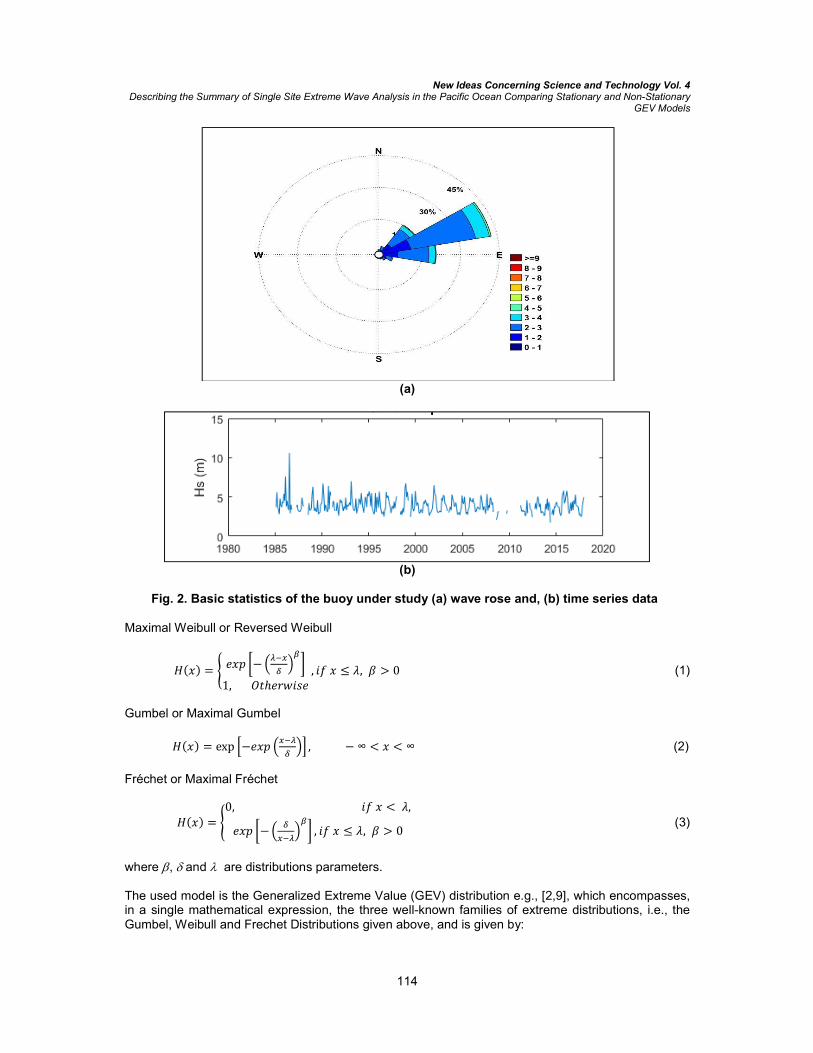
New Ideas Concerning Science and Technology Vol. 4 Describing the Summary of Single Site Extreme Wave Analysis in the Pacific Ocean Comparing Stationary and Non-Stationary
GEV Models
114
(a)
(b)
Fig. 2. Basic statistics of the buoy under study (a) wave rose and, (b) time series data
Maximal Weibull or Reversed Weibull
�(�) = ���� �− �
���
��
�
�
1, ��ℎ������
� , �� � ≤ �, � > 0 (1)
Gumbel or Maximal Gumbel
�(�) = exp �−��� ����
��� , − ∞ < � < ∞ (2)
Fréchet or Maximal Fréchet
�(�) = �
0, �� � < �,
��� �− ��
����
�
� , �� � ≤ �, � > 0� (3)
where , and are distributions parameters. The used model is the Generalized Extreme Value (GEV) distribution e.g., [2,9], which encompasses, in a single mathematical expression, the three well-known families of extreme distributions, i.e., the Gumbel, Weibull and Frechet Distributions given above, and is given by:

New Ideas Concerning Science and Technology Vol. 4 Describing the Summary of Single Site Extreme Wave Analysis in the Pacific Ocean Comparing Stationary and Non-Stationary
GEV Models
115
0expexp)(
01exp)(
1
xxG
xxG
(4)
The PDF is defined by means of
�(�) =�
��1 + � �
���
���
�
������� �
��� �− �1 + � ����
���
�
����
� �� � ≠ 0
�(�) =�
���� �−
���
�� ��� �− ��� �−
���
��� �� � = 0 (5)
where −∞ <μ < ∞ is the location parameter, ψ > 0 is the scale parameter and ξ the shape parameter. To develop the model, the lack of data should be accounted for, since this issue affects the parameters estimation stability for the extreme value distribution. Therefore, since it is known that data for some years may be absent (e.g., due to buoys maintenance), a minimum of data per time unit is considered to define the maximum values, by adopting the criterion of rejecting maximum monthly events with data blank spaces of up to 40% e.g. [5]. 3.2.2 Non-stationary GEV model
For modelling Hs the GEV is used for block maxima of a time interval. In this study, the monthly maximum values are used for the extreme value samples. Note that throughout this study, the methodology used and referenced by [5] is followed.
The seasonality is defined as the cyclic changes during the year. Usually, this cycle is linked to established climatic patrons; consequently, it repeats itself for many years and behaves in a sinusoidal way, as shown in Fig. 3. In Fig. 3 the marine weather variation is exhibited; in the winter the wave heights are larger than in the spring.
For the assessment of time-dependency an extension of traditional stationary models in extreme value theory is used. In this case the successive monthly maxima are considered as independent random variables, disregarding the need of the homogeneity hypothesis for the consecutive months, because they do not have identical distributions. It is assumed that the maximum monthly value Zt of the observed Hs in month t follows a GEV distribution, where the location μ(t)>0, scale ψ(t)>0 and shape ξ (t) parameters are time-dependent.
The cumulative distribution function (CDF) of Zi is given by
��(�) = ����� �− �1 + �(�) �
���(�)
�(�)��
�
��
�(�)��
��� �− ��� �− ����(�)
�(�)���
� (6)
The non-stationarity of the models is introduced in the GEV parameters as:

New Ideas Concerning Science and Technology Vol. 4 Describing the Summary of Single Site Extreme Wave Analysis in the Pacific Ocean Comparing Stationary and Non-Stationary
GEV Models
116
� =
⎩⎪⎪⎨
⎪⎪⎧
�(�) = �� + �� ���(2��) + �����(2��)
+�� ���(4��) + �����(4��)
�(�) = �� + �� ���(2��) + �����(2��)
+�� ���(4��) + �����(4��)
�(�) = �� + �� ���(2��) + �����(2��)
+�� ���(4��) + �����(4��)
� (7)
Where, �(� > 0) , 00 , y 0 are mean values, ii , and i (for i=1,2) are the harmonic
amplitudes; ii , and i (for i=3,4) are the subharmonic amplitudes and t is in years.
In Fig. 4 the results from the variability analysis within a year of the maximum-likelihood estimators for the location, μ, scale, ψ, and shape, ξ, parameters along the year are depicted. The circles represent the values computed with the stationary GEV model, month to month, and the line is the resulting function from the regression fitting with two harmonics. The location parameter exhibits maximum values in winter season, which indicates, in general terms, larger wave heights in November, December, January and February.
Fig. 3. Seasonality of monthly maxima
Fig. 4. Estimators for distribution parameters month to month by regression fitting

New Ideas Concerning Science and Technology Vol. 4 Describing the Summary of Single Site Extreme Wave Analysis in the Pacific Ocean Comparing Stationary and Non-Stationary
GEV Models
117
3.2.3 Non-stationary model fitting
To estimate the regression coefficients and the probability distribution parameters, the method of maximum likelihood (MML) is employed.
This method is based in the search for point estimators () for the parameters of a X function, so that the probability of observing the sample data {x1,…xn} is maximum. The likelihood function L(x;θ) is the joint density function associated to all initial extreme values, from a previously selected distribution and, in general terms, is given by
�(�; �) = �(��, . . . ��; �) = ∏ �(��; �)���� (8)
The location μ(t)>0, scale ψ(t)>0 and shape ξ (t) parameters are expressed in terms of harmonic functions, whose amplitudes are regression parameters to be mathematically estimated [10]. For our study the specific maximum likelihood function is given by
it
i
iii
i
iii
ii
m
iii
t
txt
t
txt
ttxtl
1
111log11(log|
(9)
3.2.4 Automatic selection, confidence intervals and return period values
To find the best model, a selective search methodology named Stepwise is carried out [5]. Standard errors and confidence intervals are used to deal with the uncertainty. Finally, with regard to the values associated to a return period of interest, the following equations are adopted
0)()1log(log)()(
0)()1log(1)(
)()(
)(),(),(,
)(
tifqtt
tifqt
tt
tttXtX
t
(10)
where q is the exceedance probability.
3.3 Discussion
3.3.1 Stationary model
For the stationary model the location, scale and shape parameters, which are invariant in time, are obtained. Table 1 lists the computed values of these parameters, the maximum recorded significant wave height, and the projected value for Hs associated to a return period of 30 years.
Table 1. Parameters for the stationary model, Hsmax and Hs and Tr=30 years Hsmax (m) 10.60 Hs (m) for Tr= 30 yr 5.60 � 360.34 � 58.59 � 1x10
-4
From Table 1, it can be inferred that the stationary model is dominated by a Frechet type distribution. Note that in Table 1, Hsmax = 10.60 m is an atypical value recorded on 23 July, 1986 during hurricane Estelle. It can be clearly observed in Fig. 5.
In Fig. 5 instantaneous quantiles for 30 years for the location and scale parameters are shown, the depiction corresponds to the stationary GEV over the monthly extreme values distributed month to month along the year; dots indicate the monthly maximum Hs; the red line the time-dependent quantile for a 30-year return period; the black, green and yellow lines location, scale and shape parameters, respectively.

New Ideas Concerning Science and Technology Vol. 4 Describing the Summary of Single Site Extreme Wave Analysis in the Pacific Ocean Comparing Stationary and Non-Stationary
GEV Models
118
QQ and probability Plots are shown in Fig. 6; for buoy 51004 the probability paper implies an adequate fit for the data.
Fig. 5. Estimated quantile values for Tr=30 years, monthly maximums and location, scale and shape parameters
(a) (b)
Fig. 6. (a) Probability and (b) quantile plots for the stationary GEV model
3.3.2 Non stationary model For the non-stationary model, it was found that values for the annual and semiannual cycles for the location and scale parameters are present, as well as the annual cycle for the shape parameter. The zero positive gamma value indicates that data exhibit a heavy-tailed Frechet type distribution, which is expected, if it is considered that the buoy maximum value is related to a hurricane activity, which is quite large as compared to the regular maximum recoded waves. Using the computed numerical values in the non-stationary GEV distribution equations, the best fitted parameters for the distribution are obtained. In Fig. 7 the red line shows the time-dependent quantile associated to a 30-year return period; the black line depicts the location parameter, the green line corresponds to the scale parameter and the yellow line corresponds to the shape parameter. The monthly maxima for Hs are shown by the black dots. An adequate fit for the studied case can be observed in Fig. 7. Note that the maximum Hs associated to hurricane Estelle (mentioned previously), does not significantly deviate the trend of the values associated to a 30-year return period. Nevertheless, it may lead to a smoother curve as compared with the trend for buoys in the Gulf of Mexico, where two peaks associated to cold fronts and hurricanes are shown; Fig. 7 also seems to show that kind of behavior, but the peaks may be somehow attenuated due to the atypical maximum Hs in July. Nevertheless, a seasonality effect does exist also in the Pacific Coast; it could be preliminarily concluded that seasonal trends are existent in both, the Gulf of Mexico and the Pacific Ocean.

New Ideas Concerning Science and Technology Vol. 4 Describing the Summary of Single Site Extreme Wave Analysis in the Pacific Ocean Comparing Stationary and Non-Stationary
GEV Models
119
In Fig. 8; the probability associated to the Gumbel distribution from the W(t) statistic is shown.
Fig. 7. Fitting for the monthly maximum for the non-stationary GEV model
(a) (b)
Fig. 8. Diagnostic plots (a and b) for the non-stationary GEV model
3.3.3 Comparison of stationary versus non-stationary GEV models In this section a comparison of the two employed models for the extreme value analysis is carried out. The basic stationary GEV model and the non-stationary GEV model. In Fig. 9 the most adequate fitting of the non-stationary GEV model to the data can be clearly observed, since the curve follows the seasonal trends; conversely, it can be seen that the stationary GEV model is unable to capture the seasonality of the significant wave heights. Fig. 10 shows also the best fitted results month-to-month, but for a 100-year return period. Fig. 11 shows 95% confidence intervals, where it can be observed that the bounds are more reduced for the non-stationary model and better correlated to the month-to month data. Results in Figs. 10 and 11 show the advantage of using the non-stationary GEV model, since the computed seasonal trend tend to capture the maximum values and fits better the data series. This is important, because extreme wave heights are applied to different engineering fields, for instance to offshore engineering applications [11].

New Ideas Concerning Science and Technology Vol. 4 Describing the Summary of Single Site Extreme Wave Analysis in the Pacific Ocean Comparing Stationary and Non-Stationary
GEV Models
120
A final Figure in this study, Fig. 12, shows that the best behavior (in terms of representing the selected meteo-oceanographic variable) for the used empirical data is obtained with the non-stationary GEV distribution, at least for the selected buoy, as observed by the goodness-of-fit for both models in Fig. 12 (left side column for the stationary model and right side column for the non-stationary model, respectively).
(a) (b) Fig. 9. Quantiles associated to 30-year return period for (a) the stationary and (b) non-
stationary GEV models
Fig. 10. Quantiles comparison for 100-year return period and measured Hs

New Ideas Concerning Science and Technology Vol. 4 Describing the Summary of Single Site Extreme Wave Analysis in the Pacific Ocean Comparing Stationary and Non-Stationary
GEV Models
121
Fig. 11. 30-year return period quantile and 95% confidence interval for the non-stationary GEV model and the month-to-month stationary GEV
Fig. 12. Goodness-of-fit plots for stationary (a) and non-stationary (b) models 4. CONCLUSION In this study a methodology for fitting empirical meteo-oceanographic data to extreme value models for projections purposes is published as a summary of a book chapter, based on a previous study. The selected meteo-oceanographic variable is significant wave height. The GEV model is used from two perspectives: stationarity and non-stationarity. A comparison is carried out between the two approaches for a single site. For the non-stationary GEV model the seasonality is model by means of sinusoidal curves for a single buoy in the Pacific Ocean. From the comparison of the stationary and non-stationary GEV models, it is concluded that the later leads to a better representation of the significant wave height, and also leads to larger projected return period values than the former for winter season. It is also concluded that, at least for the selected buoy and its recorded data, a seasonality trend is found, as it was the case for the Gulf of Mexico [5], although some differences are found in the trends. Future studies for more buoys and wider regions are desirable, to characterized extreme wave activity, aimed at improving the design and management of coasts and ports by including seasonality.
ACKNOWLEDGEMENTS The financial support from the Erasmus Mundus Coastal and Marine Engineering and Management (CoMEM) programme and from Universidad de Guanajuato is gratefully acknowledged. We are thankful for the comments, suggestions and constructive criticism from two anonymous reviewers.

New Ideas Concerning Science and Technology Vol. 4 Describing the Summary of Single Site Extreme Wave Analysis in the Pacific Ocean Comparing Stationary and Non-Stationary
GEV Models
122
We are also very thankful to Ms. Ruma Bag and the Editorial team for their invitation and help in the editorial process.
COMPETING INTERESTS Authors have declared that no competing interests exist.
REFERENCES 1. Shao Z, Liang B, Li H, Lee D. Study of sampling methods for assessment of extreme significant
wave heights in the South China Sea. Ocean Eng. 2018;168:173-184. DOI: 10.1016/j.oceaneng.2018.09.015.
2. Coles SG. An introduction to statistical modelling of extreme values. 1st ed.; Springer-Verlag: London, UK. 2001;1-208.
3. Katz RW. Stochastic modeling of hurricane damage. J. of App. Meteor. 2002;41:754-762. 4. Johathan P, Ewans K. Statistical modelling of extreme ocean environments for marine design:
A review. Ocean Eng. 2013;91-109 DOI: 10.1016/j.oceaneng.2013.01.004
5. Calderón-Vega F, Vázquez-Hernández AO, García-Soto AD. Analysis of extreme waves with seasonal variation in the Gulf of Mexico using a time-dependent GEV model. Ocean Eng. 2013;73:68-82. DOI: 10.1016/j.oceaneng. 2013.08.007
6. Sanchez-Arcilla A, Sierra JP, Gracia V, Garcia M, Jimenez JA, Mösso C, Valdemoro H. Coastal sustainability for uncertain futures: A spanish mediterranean case from the RISES-AM project. A: Intenational Association for Hydraulic Research Congress. E-proceedings of the 36
th IAHR
World Congres. L’Haia. 2015;1-8. 7. Sanchez-arcilla A, Sierra JP, Mösso C, Gracia V, Garcia M. Progress on climate change
detection and projections over Spain since the findings of the IPCC AR5. International Symposium CLIMATE-ES. 2015;146.
8. Peng Q, Jin S. Significant wave height estimation from space-borne cyclone-GNSS reflectometry. Remote Sensing. 2019;11(5):584.
9. Castillo E, Hadi AS, Balakrishnan N, Sarabia JM. Extreme value and related models with applications in engineering and science. Wiley-Interscience. New Jersey; 2005.
10. Menéndez M, Méndez FJ, Izaguirre C, Luceño A, Losada IJ. The influence of seasonality on estimating return values of significant wave height. Ocean Eng. 2009;56:211-219. DOI: 10.1016/j.coastaleng.2008.07.004.
11. Panchang V, Kwon Jeong Ch, Demirbilek Z. Analyses of extreme wave heights in the Gulf of Mexico for offshore engineering applications. J Offshore Mech Arct. 2013;135(3):1-15.

New Ideas Concerning Science and Technology Vol. 4 Describing the Summary of Single Site Extreme Wave Analysis in the Pacific Ocean Comparing Stationary and Non-Stationary
GEV Models
123
Biography of author(s)
F. Calderón-Vega Department of Civil Engineering, Universidad de Guanajuato, Juárez 77, Zona Centro, P.C. 36000 Guanajuato, Gto. Mexico and Laboratori d’Enginyeria Marítima, Universitat Politècnica de Catalunya, Jordi Girona 1-3, Mòdul D1, Campus Nord, 08034, Barcelona, Spain. She is a Ph.D. Candidate at the Polytechnic University of Catalunya, BarcelonaTech. She is a Researcher at the University of Guanajuato in Guanajuato, Mexico. Her research interests include maritime engineering and structures, hydraulics, extreme value theory applied to meteo-oceanographic variables and others. She has published several technical papers in international journals.
C. Mösso Laboratori d’Enginyeria Marítima, Universitat Politècnica de Catalunya, Jordi Girona 1-3, Mòdul D1, Campus Nord, 08034, Barcelona, Spain and Centre Internacional d'Investigació dels Recursos Costaners, Jordi Girona 1-3, Mòdul D1, Campus Nord, 08034, Barcelona, Spain. He is a Researcher at the Department of Civil and Environmental Engineering (hydraulics, maritime and environmental Section) at the Universitat Politècnica de Catalunya (UPC) BarcelonaTech, as well as in the Laboratori d'Enginyeria Marítima (LIM/UPC). His research interests include coastal engineering, climate change, maritime hydrodynamics among others. He has published several technical papers in international journals.
A. D. García-Soto Department of Civil Engineering, Universidad de Guanajuato, Juárez 77, Zona Centro, P.C. 36000 Guanajuato, Gto. Mexico. He is a Researcher at the University of Guanajuato in Guanajuato, Mexico. He holds a Ph.D. degree from the University of Western Ontario and a master’s degree from UNAM, Mexico. His research interests include structural reliability, live loads on bridges, seismic hazard and others. He has published several technical papers in international journals.

New Ideas Concerning Science and Technology Vol. 4 Describing the Summary of Single Site Extreme Wave Analysis in the Pacific Ocean Comparing Stationary and Non-Stationary
GEV Models
124
E. Delgadillo-Ruiz Department of Civil Engineering, Universidad de Guanajuato, Juárez 77, Zona Centro, P.C. 36000 Guanajuato, Gto. Mexico. He is currently a research professor at the University of Guanajuato Mexico. He has a Ph.D. in engineering with a terminal line in physical process modelling. His lines of research include the modelling of the components of the surface and underground water balance, as well as the study of the effects of global climate change. In addition, he belongs to the water resources and environmental engineering research group of the civil and environmental engineering department of the University of Guanajuato.
_________________________________________________________________________________ © Copyright (2021): Author(s). The licensee is the publisher (Book Publisher International).
DISCLAIMER This chapter is an extended version of the article published by the same author(s) in the following journal. Current Journal of Applied Science and Technology, 32(6): 1-12, 2019. Reviewers’ Information (1)Dr. Olumide Adesina, Olabisi Onabanjo University, Nigeria. (2)Zlatin Zlatev, Trakia University, Bulgaria.

130
APENDIX

131
Paper C
Single Site Extreme Wave Analysis in the Pacific Ocean Comparing Stationary and Non-stationary GEV Models. Current Journal of Applied Science and Technology. Calderón-Vega, C. Mösso, A. D. García-Soto and E. Delgadillo-Ruiz Current Journal of Applied Science and Technology. 32(6): 1-12, 2019; Article no.CJAST.47420

_____________________________________________________________________________________________________ *Corresponding author: E-mail: [email protected], [email protected]
Current Journal of Applied Science and Technology 32(6): 1-12, 2019; Article no.CJAST.47420 ISSN: 2457-1024 (Past name: British Journal of Applied Science & Technology, Past ISSN: 2231-0843, NLM ID: 101664541)
Single Site Extreme Wave Analysis in the Pacific Ocean Comparing Stationary and Non-stationary
GEV Models
F. Calderón-Vega1,2*, C. Mösso2,3, A. D. García-Soto1 and E. Delgadillo-Ruiz1
1Department of Civil Engineering, Universidad de Guanajuato, Juárez 77, Zona Centro, P.C. 36000 Guanajuato, Gto, Mexico.
2Laboratori d’Enginyeria Marítima, Universitat Politècnica de Catalunya, Jordi Girona 1-3, Mòdul D1,
Campus Nord, 08034, Barcelona, Spain. 3Centre Internacional d'Investigació dels Recursos Costaners, Jordi Girona 1-3, Mòdul D1, Campus
Nord, 08034, Barcelona, Spain.
Authors’ contributions
This work was carried out in collaboration between all authors. All authors designed the study, performed the statistical analysis, wrote the protocol, wrote the first draft of the manuscript, managed
the analyses of the study and managed the literature searches. All authors read and approved the final manuscript.
Article Information
DOI: 10.9734/CJAST/2019/v32i630038
Editor(s): (1) Dr. Vyacheslav O Vakhnenko, Professor, Division of Geodynamics of Explosion, Subbotin Institute of Geophysics, National
Academy of Sciences of Ukrainian, Ukraine. (2) Dr. João Miguel Dias, Assistant Professor, Habilitation in Department of Physics, CESAM, University of Aveiro, Portugal.
Reviewers: (1) Dr. Olumide Adesina, Olabisi Onabanjo University, Nigeria.
(2) Zlatin Zlatev, Trakia University, Bulgaria. Complete Peer review History: http://www.sdiarticle3.com/review-history/47420
Received 25 October 2018 Accepted 09 February 2019 Published 23 February 2019
ABSTRACT
The adequate knowledge of the weather behavior is very important for the design and management of socioeconomical, environmental and sustainability human interests in the coasts and oceans. In the present study an extreme value analysis of maximum significant waves recorded at a buoy located in the Pacific Ocean was carried out. The analysis was carried out from two perspectives, by considering a Generalized Extreme Value (GEV) model with stationary distribution (i.e., the time variations are not accounted for), and by considering a non-stationary GEV model, which incorporates the monthly seasonality of maximum observed values in time increments; the
Original Research Article

Calderón-Vega et al.; CJAST, 32(6): 1-12, 2019; Article no.CJAST.47420
2
maximum significant wave behavior was parameterized using harmonic functions for the distribution measures. Both approaches were compared for a single buoy. In the study a seasonality effect was found, which was also present at the Gulf of Mexico in previous studies, and which cannot be captured by a stationary model.
Keywords: GEV model; stationary; non-stationary; seasonality; projections. 1. INTRODUCTION The use of the extreme value theory has been widely extended in recent years to meteo-oceanographic variables. In a recent study, [1] used the Gumbel probability density function (PDF) together with maximum annual values to assess the extreme maximum annual significant wave height for projection purposes. [2] used non-stationary GEV models for investigating period trends in extreme waves. [3] developed design values for significant wave height accounting for direction and seasonality by means of a non-stationary model. [4] compared the behavior of tropical cyclone data (extreme values), obtained through simulations, versus those recorded at buoys located in the Meridional Chinese Sea and the Oriental Chinese Sea, and proposed an approach combining the set of data. [5] used peak over threshold (POT) methods and block maxima for the assessment of return values for significant wave heights. The Extreme value theory encompass methods and techniques to quantify and model the stochastic behavior, in terms of magnitude as well as in terms of frequency, of extreme events. [6,7] already mentioned the size effect on the materials strength, and in 1922 [8] introduced the concept of extreme values, while [9] studied the maximum and minimum distributions for a sample, problem which also [10] approached for normal samples. A keystone in the development of extreme value analysis was given by [11] and [12], who demonstrated that only three limiting parametric distribution families for maximum (and their minimum counterparts) are possible. [13], [14,15,16] and [17], worked on the problem of maximum and minimum distributions for a sample and found the generalized proof for [18] on the extremes type theorem. Gumbel [19] published the book "Statistics of extremes", one of the greatest contributions in the history of extreme value statistics. Later on, [20] and [21] incorporated the dependency and related results for the multivariate case. [22] and [23] described the weather variability in the geophysical variables of events.
More recently [24] referred to the Bayesian inference for modelling extreme values of characteristic marine environments and for designing maritime structures. Calderón-Vega et al. [25] investigated the seasonality of extreme waves in the Gulf of Mexico; it was found that, for the Gulf of Mexico, there is indeed seasonality effects on the extreme values; moreover, two clear peaks were found which are associated to hurricanes and cold fronts in distinctives seasons of the year. The study was carried out for several buoy sites in the Gulf of Mexico, but it was not performed for buoys in the Pacific. The use of stationary models is very common when carrying out analyses of extremes, however, as already mentioned and found in a previous study [25], seasonality may play a role in the probabilistic characterization of meteo-oceanographic variables, and it may also have an impact on design, management and reliability-oriented tasks; furthermore, since meteo-oceanographic variables are directly linked to climate change detection, vulnerability, future projection and sustainability of coasts and coastal infrastructure [26,27], an impact due to seasonality effects would be expected on all these issues for extreme waves. Although not pursued in the present study, the relation between extreme wave heights and sustainability (using stationary versus non-stationary models) could be explored in future projects; the present study can be considered as a first step in that direction. The main objective of this study is to select a single buoy site to compare stationary versus non-stationary GEV models for significant wave height projections and to inspect possible seasonality effects in the Pacific Coast for this meteo-oceanographic variable.
2. DATA USED Significant wave data recorded at 51004 buoy located at the Pacific Ocean are analyzed; the buoy is operated by the National Data Buoy Center (NDBC, www.ndbc.noaa.gov).

Calderón-Vega et al.; CJAST, 32(6): 1-12, 2019; Article no.CJAST.47420
3
Fig. 1 shows the buoy location and general information. The 51004 buoy geographical coordinate are 17.602N 152.395W, and is located to the south of the Hawaii islands. It comprises a time window from 1984 to 2017 including all years, except 2010. The significant wave height (Hs) is obtained as the mean of the highest third for wave heights during a given sample time period, which is 20 minutes for the used NDBC data. The NDBC Hs is preliminarily processed for uniformizing the data series, so that they can be employed in the probabilistic model.
3. RESULTS AND DISCUSSION 3.1 Preliminary Analysis A preliminary analysis of the data is carried out to broadly inspect the behavior of the variable under study at the selected site. In Fig. 2a (upper part) a main wave incidence to the NEE is observed. The maximum recorded Hs is equal to 10.60 m; see Fig. 2b (lower part). The most frequently observed significant wave height fluctuates around 2 m.
Fig. 1. NOAA 51004 buoy
(a)
(b)
Fig. 2. Basic statistics of the buoy under study (a) wave rose and, (b) time series data

Calderón-Vega et al.; CJAST, 32(6): 1-12, 2019; Article no.CJAST.47420
4
3.2 Extreme Value Model 3.1.1 GEV model The governing equations for the extreme value theory (EVT) can be found in [28] and they are used to establish feasible limit distributions for maxima. The only non-degenerate family of distributions obtained from EVT are the well-known Weibull, Gumbel and Fréchet families for maxima, and they are given below [28].
Maximal Weibull or Reversed Weibull
�(�) = ���� �− �
���
��
�
�
1, ��ℎ������
� , �� � ≤ �, � > 0 (1)
Gumbel or Maximal Gumbel
�(�) = exp �−��� ����
��� , − ∞ < � < ∞
(2) Fréchet or Maximal Fréchet
�(�) = �
0, �� � < �,
��� �− ��
����
�
� , �� � ≤ �, � > 0�
(3) where , and are distributions parameters. The used model is the Generalized Extreme Value (GEV) distribution e.g., [22,28], which encompass, in a single mathematical expression, the three well-known families of extreme distributions, i.e., the Gumbel, Weibull and Frechet Distributions given above, and is given by:
0expexp)(
01exp)(
1
xxG
xxG
(4)
The PDF is defined by means of
�(�) =�
��1 + � �
���
���
�
������� �
��� �− �1 +
��−��+−1��� �≠0
�(�) =�
���� �−
���
�� ��� �− ��� �−
���
��� �� � = 0
(5) where −∞ <μ < ∞ is the location parameter, ψ > 0 is the scale parameter and ξ the shape parameter. The location parameter represents the mean values of the random variable, x, and defines the value with a non-exceedance probability exp(-1). The scale parameter represents the sample dispersion. Finally, the shape parameter defines the distribution family as a function of the tail behavior; when ξ exists, G(x) includes two distribution families. To develop the model, the lack of data should be accounted for, since this issue affects the parameters estimation stability for the extreme value distribution. Therefore, since it is known that data for some years may be absent (e.g., due to buoys maintenance), a minimum of data per time unit is considered to define the maximum values, by adopting the criterion of rejecting maximum monthly events with data blank spaces of up to 40% e.g. [25]. 3.1.2 Non-stationary GEV model For modelling Hs the GEV is used for block maxima of a time interval. In this study, the monthly maximum values are used for the extreme value samples. Note that throughout this study, the methodology used and referenced by [25] is followed. The seasonality is defined as the cyclic changes during the year. Usually, this cycle is linked to established climatic patrons; consequently, it repeats itself for many years and behaves in a sinusoidal way, as shown in Fig. 3. In Fig. 3 the marine weather variation is exhibited; in the winter the wave heights are larger than in the spring.
For the assessment of time-dependency an extension of traditional stationary models in extreme value theory is used. In this case the successive monthly maxima are considered as independent random variables, disregarding the need of the homogeneity hypothesis for the consecutive months, because they do not have identical distributions. It is assumed that the maximum monthly value Zt of the observed Hs in month t follows a GEV distribution, where the location μ(t)>0, scale ψ(t)>0 and shape ξ (t) parameters are time-dependent.

Calderón-Vega et al.; CJAST, 32(6): 1-12, 2019; Article no.CJAST.47420
5
The cumulative distribution function (CDF) of Zi is given by
��(�) = ����� �− �1 + �(�) �
���(�)
�(�)��
�
��
�(�)��
��� �− ��� �− ����(�)
�(�)���
�
(6) The non-stationarity of the models is introduced in the GEV parameters as:
� =
⎩⎪⎪⎨
⎪⎪⎧
�(�) = �� + �� ���(2��) + �����(2��)
+�� ���(4��) + �����(4��)
�(�) = �� + �� ���(2��) + �����(2��)
+�� ���(4��) + �����(4��)
�(�) = �� + �� ���(2��) + �����(2��)
+�� ���(4��) + �����(4��)
�
(7)
Where, �(� > 0) , 00 , y 0 are mean
values, ii , y i (for i=1,2) are the harmonic
amplitudes; ii , y i (for i=3,4) are the
subharmonic amplitudes and t is in years.
In Fig. 4 the results from the variability analysis within a year of the maximum-likelihood estimators for the location, μ, scale, ψ, and shape, ξ, parameters along the year are depicted. The circles represent the values computed with the stationary GEV model, month to month, and the line is the resulting function from the regression fitting with two harmonics.
The location parameter exhibits maximum values in winter season, which indicates, in general terms, larger wave heights in November, December, January and February.
Fig. 3. Seasonality of monthly maxima
Fig. 4. Estimators for distribution parameters month to month by regression fitting

Calderón-Vega et al.; CJAST, 32(6): 1-12, 2019; Article no.CJAST.47420
6
3.1.3 Non-stationary model fitting
To estimate the regression coefficients and the probability distribution parameters, the method of maximum likelihood (MML) is employed. This method is based in the search for point estimators () for the parameters of a X function, so that the probability of observing the sample data {x1,…xn} is maximum. The likelihood function L(x;θ) is the joint density function associated to all initial extreme values, from a previously selected distribution and, in general terms, is given by
�(�; �) = �(��, . . . ��; �) = ∏ �(��; �)�
��� (8)
The location μ(t)>0, scale ψ(t)>0 and shape ξ (t) parameters are expressed in terms of harmonic functions, whose amplitudes are regression parameters to be mathematically estimated [29]. For our study the specific maximum likelihood function is given by
it
i
iii
i
iii
ii
m
iii
t
txt
t
txtttxtl
1
111log11(log|
(9)
3.1.4 Automatic selection, confidence intervals and return period values
To find the best model, a selective search methodology named Stepwise is carried out; the Stepwise is in turn based on combining two approaches denoted “Forward Selection” and “Backward Elimination”. Any probabilistic model should ideally incorporate some measure of uncertainty to evaluate the randomness or error from the selected model; for the present study standard errors and confidence intervals are used to deal with the uncertainty. Finally, with regard to the values associated to a return period of interest, the following equations are adopted,
0)()1log(log)()(
0)()1log(1)(
)()(
)(),(),(,
)(
tifqtt
tifqt
tt
tttXtX
t
(10)
where q is the exceedance probability defined from G t(x)=1-q and the estimated quantile, and
Xq(t,θ) is the time-dependent value associated to the return period R=1/q. A more detailed description can be found in the study by [25] and the references cited in that paper.
4. DISCUSSION 4.1 Stationary Model For the stationary model the location, scale and shape parameters, which are invariant in time, are obtained. Table 1 lists the computed values of the distribution parameters, as well as the maximum recorded significant wave height, Hsmax, and the projected value for Hs associated to a return period of 30 years.
Table 1. Parameters for the stationary model,
Hsmax and Hs and Tr=30 years
Hsmax (m) 10.60 Hs (m) for Tr= 30 yr 5.60
� 360.34 � 58.59 � 1x10⁻⁴
From the values reported in Table 1, it can be inferred that the stationary model is dominated by a Frechet type (heavy tail) distribution behavior. Note that in Table 1, Hsmax = 10.60 m is an atypical value recorded on 23 July, 1986 during hurricane Estelle (http://www.prh.noaa.gov/cphc/summaries/1986.php); it can be clearly observed in Fig. 5. In Fig. 5 the instantaneous quantiles for a return period of 30 years for the location and scale parameters are shown, the depiction corresponds to the stationary GEV over the monthly extreme values distributed month to month along the year. In Fig. 5, dots indicate the monthly maximum Hs; the red line represents the time-dependent quantile associated to a 30-year return period; the black, green and yellow lines depict the location, scale and shape parameters, respectively.
In addition to the previous figure, QQ and probability Plots are shown in Fig. 6, where it can be observed that for buoy 51004 the probability paper implies an adequate fit for the data; nonetheless, the QQ plot underestimates the quantiles of the extreme values.

Calderón-Vega et al.; CJAST, 32(6): 1-12, 2019; Article no.CJAST.47420
7
Fig. 5. Estimated quantile values for Tr=30 years, monthly maximums and location, scale and shape parameters
(a) (b)
Fig. 6. (a) Probability and (b) quantile plots for the stationary GEV model
Fig. 7. Fitting for the monthly maximum for the non-stationary GEV model
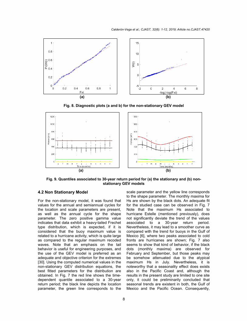
Calderón-Vega et al.; CJAST, 32(6): 1-12, 2019; Article no.CJAST.47420
8
(a) (b)
Fig. 8. Diagnostic plots (a and b) for the non-stationary GEV model
(a) (b)
Fig. 9. Quantiles associated to 30-year return period for (a) the stationary and (b) non-
stationary GEV models
4.2 Non Stationary Model
For the non-stationary model, it was found that values for the annual and semiannual cycles for the location and scale parameters are present, as well as the annual cycle for the shape parameter. The zero positive gamma value indicates that data exhibit a heavy-tailed Frechet type distribution, which is expected, if it is considered that the buoy maximum value is related to a hurricane activity, which is quite large as compared to the regular maximum recoded waves. Note that an emphasis on the tail behavior is useful for engineering purposes, and the use of the GEV model is preferred as an adequate and objective criterion for the extremes [30]. Using the computed numerical values in the non-stationary GEV distribution equations, the best fitted parameters for the distribution are obtained. In Fig. 7 the red line shows the time-dependent quantile associated to a 30-year return period; the black line depicts the location parameter, the green line corresponds to the
scale parameter and the yellow line corresponds to the shape parameter. The monthly maxima for Hs are shown by the black dots. An adequate fit for the studied case can be observed in Fig. 7 Note that the maximum Hs associated to hurricane Estelle (mentioned previously), does not significantly deviate the trend of the values associated to a 30-year return period. Nevertheless, it may lead to a smoother curve as compared with the trend for buoys in the Gulf of Mexico [6], where two peaks associated to cold fronts are hurricanes are shown; Fig. 7 also seems to show that kind of behavior, if the black dots (monthly maxima) are observed for February and September, but those peaks may be somehow attenuated due to the atypical maximum Hs in July. Nevertheless, it is noteworthy that a seasonality effect does exists also in the Pacific Coast and, although the results in the present study are limited to one site only, it could be preliminarily concluded that seasonal trends are existent in both, the Gulf of Mexico and the Pacific Ocean. Consequently,

Calderón-Vega et al.; CJAST, 32(6): 1-12, 2019; Article no.CJAST.47420
9
further studies to compare the trends for more buoys in the Pacific are strongly recommended.
To represent the adequacy of the fitting, the empirical probabilities obtained with the model and with the quantiles are shown in Fig. 8; the probability associated to the Gumbel distribution from the W(t) statistic is shown.
4.3 Comparison of Stationary Versus Non-stationary GEV Models
In this section a comparison of the two employed models for the extreme value analysis is carried out. The basic stationary GEV model and the non-stationary GEV model, which, unlike the former, captures seasonal variation for monthly maxima data series, are contrasted. In Fig. 9 the most adequate fitting of the non-stationary GEV model to the data can be clearly observed, since the curve follows the seasonal trends; conversely, it can be seen that the stationary GEV model is unable to capture the seasonality of the significant wave heights. Fig. 10 shows also the best fitted results month-to-month, but for a 100-year return period. In Fig. 10 the depicted quantile for a 100-year return period shows that the non-stationary model includes the extreme values and represents more adequately the seasonality of the used data (red line), as compared to the stationary model (green line), except by the extreme value in July (see black dots for monthly Hs). Fig. 11 shows 95% confidence intervals, where it can be observed that the bounds are more reduced for the non-stationary model and better correlated to the month-to month data.
Results in Figs. 10 and 11 show the advantage of using the non-stationary GEV model, since the computed seasonal trend tend to capture the maximum values and fits better the data series; the expected wave heights for TR=100 years computed for the non-stationary case are larger than those computed with the stationary one for the winter season, and the opposite occurs for the summer season; this is important, since an impact in design, management, reliability related tasks and sustainability related issues is expected. The reason of the smaller values with the stationary GEV model for some months, is that it does not effectively account for scarce and extreme wave heights associated to hurricanes. In contrast, the non-stationary GEV model can capture these extreme values (also included in the integrated quantile) by means of the sinusoidal trend.
A final Figure in this study, Fig. 12, shows that the best behavior (in terms of representing the selected meteo-oceanographic variable) for the used empirical data is obtained with the non-stationary GEV distribution, at least for selected buoy, as observed by the goodness-of-fit for both models in Fig. 12 (left side column for the stationary model and right side column for the non-stationary model, respectively). It is pointed out once more, that this is due to the fact that the non-stationary model try to capture the majority of extreme values through a sinusoidal computing scheme; also, the existent extreme wave values caused by hurricanes, which significantly alter the seasonal periodic variation, are more adequately incorporated by the non-stationary GEV model in general terms; moreover, the uncertainty induced by hurricane activity, is compensated by the non-stationary GEV model for the monthly data series.
Fig. 10. Quantiles comparison for 100-year return period and measured Hs

Calderón-Vega et al.; CJAST, 32(6): 1-12, 2019; Article no.CJAST.47420
10
Fig. 11. 30-year return period quantile and 95% confidence interval for the non-stationary GEV model and the month-to-month stationary GEV
(a) (b)
Fig. 12. Goodness-of-fit plots for stationary (a) and non-stationary (b) models
5. CONCLUSION In this study a methodology for fitting empirical meteo-oceanographic data to extreme value models for projections purposes is presented. The selected meteo-oceanographic variable is significant wave height. The GEV model is used from two perspectives: Stationarity and non-
stationarity. A comparison is carried out between the two approaches for a single site. For the non-stationary GEV model the seasonality is model by means of sinusoidal curves for a single buoy in the Pacific Ocean. The non-stationary GEV model predicts adequately the monthly maximum significant

Calderón-Vega et al.; CJAST, 32(6): 1-12, 2019; Article no.CJAST.47420
11
wave heights and reduce the uncertainty of the estimated quantiles; it also projects in a better way the wave heights associated to given return periods, since the methodology includes not only the point maxima, but also the peripheric values along the year. From the comparison of the stationary and non-stationary GEV models, it is concluded that the later leads to a better representation of the meteo-oceanographic variable, and also leads to larger projected return period values than the former for winter season. This is important, since implications in design of maritime structures, managements tasks, reliability and risk assessments, as well as sustainability related issues, are expected depending on the selected model.
It is also concluded that, at least for the selected buoy and its recorded data, a seasonality trend is found, as it was the case for the Gulf of Mexico [6], although some differences are found in the trends. Future studies for more buoys and wider regions are desirable, to characterized extreme wave activity, aimed at improving the design and management of coasts and ports by including seasonality. It is suggested to investigate the impact of selecting different models (i.e., stationary versus non-stationary models for extreme waves) in the sustainability of coasts and coast infrastructure. Further research for other meteo-oceanographic variables is also recommended.
ACKNOWLEDGMENTS
The financial support from the Erasmus Mundus Coastal and Marine Engineering and Management (CoMEM) programme and from Universidad de Guanajuato is gratefully acknowledged. We are thankful for the comments, suggestions and constructive criticism from two anonymous reviewers.
COMPETING INTERESTS
Authors have declared that no competing interests exist.
REFERENCES
1. Shao Z, Liang B, Li H, Lee D. Study of sampling methods for assessment of extreme significant wave heights in the South China Sea. Ocean Eng. 2018;168: 173-184. DOI: 10.1016/j.oceaneng.2018.09.015
2. Vanem E. Non-stationary extreme value models to account for trends and shifts in the extreme wave climate due to climate
change. Appl Ocean Res. 2015;52:201-211.
DOI: 10.1016/j.apor.2015.06.010 3. Feld G, Randell D, Wu Y, Ewans, K,
Jonathan P. Estimation of storm peak and intrastorm directional-seasonal design conditions in the North Sea. Journal of Offshore Mechanics and Arctic Engineering. 2015;137(2):021102.
DOI: 10.1115/1.4029639 4. Shao Z, Liang B, Li H, Wu G, Wu Z.
Blended wind fields for wave modeling of tropical cyclones in the South China Sea and East China Sea. Appl Ocean Res. 2018;71:20-33.
DOI: 10.1016/j.apor.2017.11.012 5. Kapelonis Zacharias G, Gavriliadis
Panagiotis N, Athanassoulis Gerassimos A. Extreme value análisis of dynamical wave climate projections in the Mediterranean Sea. Procedia Computer Science. YSC 4Th International Young Scientists Conference on Computacional Science. 2015;66:210-219.
6. Chaplin RG. Abrasion resistant concrete floors. Advances in Concrete Slab Technology. Ed. Dhir RK, Munday JGL. 1980;164-72.
7. Chaplin RG. The influence of cement replacement materials. Fine Agregate and curing on the abrasion resistance of industrial concrete floor slabs. Cement and Concrete Association. Slough, UK. 1986; 32.
8. Bortkiewicz L, von Variationsbreite, mittlerer Fehler, Sitzungsber. Berli. Math. Ges. 1922;21:3-11.
9. Dodd EL. The greatest and the least variate under general laws of error. Tans.Amer. Math Soc. 1923;25:525-39.
10. Tippett LHC. On the extreme individuals and the range of samples taken from a normal population, Biometrika. 1925;17: 364-387 Available:https://doi.org/10.1093/biomet/17.3-4.364
11. Fréchet M. Sur la loi de probabilité de l’écart maximum, Ann. Soc. Polon. Math. Cracovie. 1957;6:93-116.
12. Fisher RA, Tippett LHC. Limiting forms of the frequency distribution of the largest or smallest members of a sample. Proceedings of the Cambridge Philosophi-cal Society.1928;24:180-190.
13. De Finetti B, Obry S. L’optimum nella misura del riscatto, Atti del II Congresso

Calderón-Vega et al.; CJAST, 32(6): 1-12, 2019; Article no.CJAST.47420
12
Nazionale di Scienza delle Assicurazioni. Bardi, Trieste, Rome. 1932;2:99–123.
14. Gumbel EJ. Statistical theory of extreme values and some practical applications. Applied Mathematics Series. 33 (1st ed.) U.S. Department of Commerce, National Bureau of Standards; 1954.
15. Gumbel EJ. Les valeurs extrêmes des distributions statistiques. Annales de l’Institut Henri Poincaré. 1935;5:115-158.
16. Mises R. von. La distribution de la plus grande de n valeurs. Amer. Math. Soc Reproduced in Selected Papers of Richard von Mises, II. 1954. 1936;271-294.
17. Rice J. Mathematical statistics and data analysis. 2
nd ed. Duxbury; 1994.
18. Gnedenko B. Sur la distribution limite du terme maximum d’une série aléatoire. Springer-Verlag. 1943;195-225.
19. Gumbel EJ. Statistics of extremes. Columbia University Press; 1958.
20. Galambos J. The asymptotic theory of extreme order statistics, Robert E. Krieger. Malabar, Florida. 2nd ed; 1987.
21. Leadbetter MR, Lindgrem G, Rootzén H. Extremes and related properties of random sequences and series. Springer. Verlag, New York; 1983.
22. Coles SG. An introduction to statistical modelling of extreme values. 1st ed.; Springer-Verlag: London, UK. 2001;1-208.
23. Katz RW. Stochastic modeling of hurricane damage. J. of App. Meteor. 2002;41:754-762.
24. Johathan P, Ewans K. Statistical modelling of extreme ocean environments for marine design: A review. Ocean Eng. 2013;91-109.
DOI: 10.1016/j.oceaneng.2013.01.004 25. Calderón-Vega F, Vázquez-Hernández
AO, García-Soto AD. Analysis of extreme waves with seasonal variation in the Gulf of Mexico using a time-dependent GEV model. Ocean Eng. 2013;73:68-82. DOI: 10.1016/j.oceaneng. 2013.08.007
26. Sanchez-Arcilla A, Sierra JP, Gracia V, Garcia M, Jimenez JA, Mösso C, Valdemoro H. Coastal sustainability for uncertain futures: A Spanish Mediterra-nean case from the RISES-AM project. A: Intenational Association for Hydraulic Research Congress. E-proceedings of the 36th IAHR World Congres. L’Haia. 2015;1-8.
27. Sanchez-arcilla A, Sierra JP, Mösso C, Gracia V, Garcia M. Progress on climate change detection and projections over Spain since the findings of the IPCC AR5. International Symposium Climatees. 2015; 146.
28. Castillo E, Hadi AS, Balakrishnan N, Sarabia JM. Extreme value and related models with applications in engineering and science. Wiley-Interscience. New Jersey; 2005.
29. Menéndez M, Méndez FJ, Izaguirre C, Luceño A, Losada IJ. The influence of seasonality on estimating return values of significant wave height. Ocean Eng. 2009; 56:211-219. DOI: 10.1016/j.coastaleng.2008.07.004
30. Panchang V, Kwon Jeong Ch, Demirbilek Z. Analyses of extreme wave heights in the Gulf of Mexico for offshore engineering applications. J Offshore Mech Arct. 2013; 135(3):1-15.
_________________________________________________________________________________ © 2019 Calderón-Vega et al.; This is an Open Access article distributed under the terms of the Creative Commons Attribution License (http://creativecommons.org/licenses/by/4.0), which permits unrestricted use, distribution, and reproduction in any medium, provided the original work is properly cited.
Peer-review history: The peer review history for this paper can be accessed here:
http://www.sdiarticle3.com/review-history/47420

143
Paper D
Analysis of extreme waves with seasonal variation in the Gulf of Mexico using a time-dependent GEV model F.Calderón-Vega, A.O.Vázquez-Hernández, A.D.García-Soto Ocean Engineering. Ocean Engineering 73 (2013) 68–82

Analysis of extreme waves with seasonal variation in the gulf of Mexicousing a time-dependent GEV model
F. Calderón-Vega a, A.O. Vázquez-Hernández b,n, A.D. García-Soto c
a Universidad de Cantabria, Avda. de los Castros s/n, 39005 Santander, Spainb Instituto Mexicano del Petróleo, Deep Waters Explotation Department, Eje Central Lázaro Cárdenas Norte 152, Gustavo A. Madero,07730 Mexico City, Mexicoc Department of Applied Mechanics, Institute of Engineering, National Autonomous University of Mexico, Mexico City, Mexico
a r t i c l e i n f o
Article history:Received 24 November 2012Accepted 24 August 2013
Keywords:Extreme wave statisticsExtreme value distributionSignificant wave heightSeasonalityGEV distribution
a b s t r a c t
This paper considers a time-dependent GEV model to assess the extreme value of significant wave. Themodel incorporates the monthly seasonality of maximum values in a block of time of recorded events.The extreme value distribution parameters are fitted considering the seasonal behavior of the significantwave height using harmonic functions representing annual and semiannual cycles. The model is appliedto the records in 10 buoys in the Gulf of Mexico. The obtained results are compared with some of theavailable results in the literature.
& 2013 Elsevier Ltd. All rights reserved.
1. Introduction
Correct characterization of the maritime climate is crucial forthe design and operation of coastal and marine infrastructure.Seasonal variation of extreme values of waves influences the riskof flooding. It also affects the design, construction, installation andoperation activities of structures such as breakwaters, ports, andoil rigs. Often the design and operation of the structures requiresthe estimation of the extreme wave height for specified returnperiods. The selection and assignment of an appropriate prob-ability distribution based on available statistical data is of para-mount importance for the estimation of the return period valuesof the wave height.
According to the asymptotic theory, the maximum values ofrandom sequences could be adequately modeled by the general-ized extreme value (GEV) distribution, which is a reformulation ofthe limiting distributions originally developed by Fisher andTippet, and later systematized by Gumbel (Chakrabarti, 2001).It is important to note that, depending on the employed statisticalmethod, the available records and the sample selection cansignificantly influence the assessment of the extreme values(Prpiĉ-Orsîc et al., 2007; Martucci et al., 2010).
Several statistical models have been proposed to adequatelyrepresent the ocean behavior considering site conditions (Isaacsonand Mackenzie, 1981; Muir and ElShaarawi, 1986; Prevosto et al.,2000; Stansell, 2005; Tayfun and Fedele, 2007; Jensen et al., 2011;Mazas and Hamm, 2011; Muraleedharan et al., 2012; Solari andLosada, 2012; Soares and Carvalho, 2012). However, only a fewstudies have focused on the seasonal variation. For example,Mietus (1998) carried out an analysis of the seasonal variationon the surface level wind speed in the Baltic Sea. Jönsson et al.(2002) showed that there is a large seasonal variation in maximummonthly wave heights in the Baltic Sea. Méndez et al. (2008)presented a statistical model to characterize the long-termextreme value distribution of significant wave height, conditionedto the duration of the storm and accounting for seasonality; theybasically used a time-dependent version of the peak over thresh-old (POT) approach to build a model that considers the annual andsemiannual cycles parameterized in terms of harmonic functions.Mackay et al. (2010) showed that estimates of extreme waveconditions from stationary models have a lower bias and variancethan those from discrete seasonal models. They also showed thatthe estimations from discrete seasonal models tend to be highlybiased. Räämet and Soomere (2010) estimated the seasonal varia-tion in wave climate in the Baltic Sea using a high-resolutionversion of a wave model.
There are some studies for extreme wave heights in the Gulfof Mexico; most of them do not consider the seasonal variation.Although Jonathan and Ewans (2011) modeled the seasonality ofextreme waves in the Gulf of Mexico using a non-homogeneous
Contents lists available at ScienceDirect
journal homepage: www.elsevier.com/locate/oceaneng
Ocean Engineering
0029-8018/$ - see front matter & 2013 Elsevier Ltd. All rights reserved.http://dx.doi.org/10.1016/j.oceaneng.2013.08.007
n Corresponding author. Tel.: þ52 55 9175 8228; fax: þ52 55 9175 8258.E-mail addresses: [email protected], [email protected]
(A.O. Vázquez-Hernández).
Ocean Engineering 73 (2013) 68–82

Poisson model, it was carried out only for two unspecifiedlocations and considering only peak significant wave heightsfor storm events. They used information from GOMOS hindcastdata (2005) instead of NOAA buoys. They employed the general-ized Pareto distribution including shape and scale parametersonly, and concluded that seasonal variation may be dependenton the location in the Gulf of Mexico. Therefore, it wouldbe desirable to carry out a study considering the seasonalvariations of extreme wave heights during the year at severalsites in the Gulf of Mexico, and to incorporate the seasonalvariability in the probabilistic model. This can be important forthe design of maritime structures, coast management, andestimation of wave loading and reliability of offshore structures(e.g. Hong, 1994).
The main objective of this study is to characterize the seasonalbehavior of extreme wave heights in the Gulf of Mexico. It uses themodel presented by Méndez et al. (2008) but with additionalterms that take into account the seasonality of the shape para-meter of the GEV (i.e., time-dependent GEV model), throughharmonic functions that represents the annual and semiannualcycles (e.g. Menéndez et al., 2009). The seasonality is the maincovariate in this work, although it is acknowledged that othercovariates such as the directionality (e.g. Jonathan and Ewans,2007) could be important but are out of the scope of this study.The estimated extremes are compared with those presented byPanchang and Li (2006).
2. Extreme time-dependent GEV distribution
The GEV distribution for maximum values in a block of time isused for modeling the significant wave height (Leadbetter et al.,1983). The GEV distribution that in the extreme cases, becomesthe well-known Gumbel, Weibull and Frechet distributions, can beexpressed as (Coles, 2001)
GðxÞ ¼ exp � 1þξx�μψ
� �� ��1=ξ
þ
( )-ξa0
GðxÞ ¼ exp �exp � x�μψ
� �� �� �-ξ¼ 0 ð1Þ
The density function is defined by:
gðxÞ ¼ 1ψ
1þξx�μψ
� �� ��ð1þ1=ξÞ
þexp � 1þξ
x�μψ
� �� �ð�1=ξÞ
þ
( )-ξa0
gðxÞ ¼ 1ψexp �x�μ
ψ
� �exp �exp � x�μ
ψ
� �� �� �-ξ¼ 0 ð2Þ
where [a]þ implies max (a, 0), �1oμo1 is the locationparameter, ψ40 is the scale parameter and ξ is the shapeparameter, which defines the type of distribution; ξa0, corre-sponds to two distribution families: Fréchet for ξ40 and Weibullξo0; when ξ-0 the GEV tends to the Gumbel distribution.
The behavior of Weibull, Frechet and Gumbel distributionsin the tail of the distribution function differs. The tails arebounded, heavy and light, for the Weibull, Frechet and Gumbeldistributions, respectively. In the Gumbel distribution the taildecays exponentially, whereas in the Fréchet distribution the taildecays as a function of a power. Only one of the three extremevalue distributions is often selected for practical applications.
In this study, a time-dependent GEV distribution model,which takes into account the seasonality using independentmonthly maximum values, xi, observed at times ti, is employed.The consideration of independent monthly maximum series isadequate because: first, the seasonality for quasi-homogeneous
time distributed data could be modeled (Mendez et al., 2007),and second, because the monthly maxima provides additionalinformation about the upper tail of the distribution (Katz et al.,2002). The model is applied to the records of wave heights fromseveral buoys located in the Gulf of Mexico and described inTable 1.
The lack of data in the series must be taken into account toapply the model, because this affects the stability of the parameterestimation for the extreme value distribution. Since there areseasons without recorded data in the series, a minimum numberof data points per unit time (or a time interval in which themaximum value is extracted) is considered. For this, the criterionproposed in Mendez et al. (2007) is adopted. This criterion statesthat the record for a month is rejected if up to 40% of data of themonth is missing.
2.1. Regression model
The seasonal variation in this study is defined as the cyclicalchanges within one year. Authors such as Morton et al. (1997), andCarter and Challenor (1981), modeled the intra-annual variabilityby analyzing the seasonal behavior of extreme wave heights usingextreme value distribution. Räämet and Soomere (2010) devel-oped a model that adequately reproduced the seasonal patterns ofwave intensity and the probability distribution functions fordifferent wave heights. Normally, the seasonal variation is linkedto established weather patterns, so it is usually recurrent over theyears and has a sinusoidal behavior. The seasonal variability forgeophysic variables is manifested in different ways. However, apredominant factor is presented in all cases: the annual cycle,generally defined by the winter–summer variability. In Fig. 1,this cycle is observed in the monthly maxima wave heights forthe shown buoys in the Gulf of Mexico. It is also observed that theannual cycle clearly defines the variable behavior along the time.The semiannual cycle is not only referred to the winter–summervariability, but also to a systematic climate pattern during the year,such as the hurricanes.
After observing the boxplots in Fig. 1, it is considered that theseasonal variability can be modeled as a superposition of sinusoi-dal waves by using harmonic functions and include them in themodel. To justify the inclusion of the seasonality in the model, theone-year variability of the location, scale and shape parameters ofthe fitted time-independent GEV for every month has beenanalyzed.
The time dependency is introduced in the model parameters inthe GEV model by employing harmonic functions defined by
Table 1Information of the buoys used in the study.
Station(Buoy)
Recordedyears
No. ofrecordedyears
No. ofmonthlymaximumvalues
MaximumrecordedSWH (m)
Distanceto shore(Km)
Waterdepth(m)
42,001 1975–2011 36 393 11.2 334 324642,002 1973–2011 33 391 9.7 346 356642,003 1976–2011 35 374 11.04 307 323342,007 1981–2009 29 183 9.09 35 1442,019 1990–2011 22 228 6.30 92 8242,020 1990–2011 22 233 8.20 68 8842,035 1993–2011 19 223 6.03 25 1642,036 1994–2011 18 194 8.60 127 5442,039 1995–2011 17 143 12.05 114 30742,040 1995–2011 17 142 16.91 79 274
F. Calderón-Vega et al. / Ocean Engineering 73 (2013) 68–82 69

(Méndez et al., 2008; Menéndez et al., 2007; Menéndez et al.,2009),
θ¼μðtÞ ¼ β0þβ1 cos ð2πtÞþβ2 sin ð2πtÞþβ3 cos ð4πtÞþβ4 sin ð4πtÞψ ðtÞ ¼ α0þα1 cos ð2πtÞþα2 sin ð2πtÞþα3 cos ð4πtÞþα4 sin ð4πtÞξðtÞ ¼ γ0þγ1 cos ð2πtÞþγ2 sin ð2πtÞþγ3 cos ð4πtÞþγ4 sin ð4πtÞ
8><>:
ð3Þwhere ψ ðt40Þ. θ includes the three parameters: location, scaleand shape (μðtÞ, ψ ðtÞ and ξðtÞ), respectively. To simplify thenotation, in the following it is considered that θ represents thevector of all the model parameters involved in Eq. (3) that are to beestimated, θ¼ ðβ0;β1;β2;β3;β4;α0;α1;α2;α3;α4; γ0;γ1;; γ2; ; γ3;γ4;Þ.Note that β0;α0 and γ0 represent the mean of (μðtÞ, ψ ðtÞ andξðtÞ); βi;αi and γi (for i¼1,2) are the amplitudes of the harmonics;βi;αi andγi (for i¼3,4) are the amplitudes of the subharmonics,and t is given in years.
2.2. Fitting to the data
Different procedures to estimate the model regression coefficients,or to estimate the probability distribution parameters are available.
In this study the maximum likelihood method has been employedfor the analysis. In general, this technique results in adequatefitting, and in less biased and more efficient estimators, especiallyfor long return periods and for small data samples (Lettenmaierand Burges, 1982). The maximum likelihood method consists inestimating the point parameter estimators of a likelihood functionso that the likelihood of observing the samples {x1,…xn} ismaximum. More specifically, the likelihood function can beexpressed as (Benjamin and Cornell, 1970)
Lðθ; x1; x2; :::; xnÞ ¼ f ðx1; :::xn;θÞ ¼ ∏n
i ¼ 1f ðxi;θÞ ð4Þ
where Lðθ; x1; x2; :::; xnÞ is the likelihood function and f ðx1; :::xn;θÞrepresents the joint probability density function conditioned onthe model parameters θ. The last equality holds if the sample isindependent and identically distributed with density functionf ðx;θÞ. To simplify the computing, Eq. (4) can be re-written as,
lðθ; x1; x2; :::; xnÞ ¼ Σn
i ¼ 1log ½f ðx1; :::xn;θÞ� ð5Þ
where the log-likelihood function lðθ; x1; x2; :::; xnÞ � log Lðθ;x1; x2; :::; xnÞ.
Fig. 1. Boxplots for monthly maxima significant wave height in 42,001, 42,002, 42,035, and 42,040 buoys. Trapezoidal boxes have lines at the lower, median and upperquartile values. The whiskers extend to the 1.5 interquartile range, and crosses show unusual values.
F. Calderón-Vega et al. / Ocean Engineering 73 (2013) 68–8270

The maximum likelihood estimators, θ, that maximizes lðθ;x1; x2; :::; xnÞ is obtained by solving
Σn
i ¼ 1
∂∂θj
log ½f ðx1; :::xn;θÞ� ¼ 0 for j¼ 1;…; p ð6Þ
where p denotes the total number of parameters to be estimated.For the GEV model shown in Eq. (2), the log-likelihood function is
lðθjti; xiÞ ¼ � ∑n
i ¼ 1
(log ψ ðtiÞþð1þ1=ξðtiÞÞlog 1þξðtiÞ
xi�μðtiÞψ ðtiÞ
� �� �þ
þ 1þξðtiÞxi�μðtiÞψ ðtiÞ
� �� �ð�1=ξðtiÞÞ
þ
)ð7Þ
where x1,…,xn are defined as the n observations of maxima for ablock of time. The obtained distribution parameters μ, ψand ξ, forthe considered wave height data are shown in Fig. 2.
It can be observed from the figure that the location parameterpresents minimum values in summer and maximum values inwinter. This means that higher wave heights occur in November,December, January and February. The scale parameter shows aharmonic behavior in all buoys, which generally has a lower valuein summer. The shape parameter is also seasonally modulated;when it is not zero and adopts positive or negative values, itindicates that the sample behaves as a Frechet or Weibulldistribution, respectively.
2.3. Uncertainty
An estimate of the uncertainty associated with the pointestimate of the distribution model parameters are given below.This estimation is carried out using Hessian matrix of � l(x;θ)evaluated at θ, known as information matrix, I0,
I0 ¼
�∂2 lðθÞ∂θ1
2 … … � ∂2 lðθÞ∂θ1∂θp
⋮ ⋱ �∂2 lðθÞ∂θi∂θj
⋮
⋮ �∂2lðθÞ∂θj∂θi
⋱ ⋮
� ∂2 lðθÞ∂θp∂θ1
… … �∂2 lðθÞ∂θp
2
26666666664
37777777775¼ ð8Þ
where p is the number of estimated parameters defining thedistribution function. The I0 matrix is asymptotically equivalentto the Fisher information matrix (the same matrix but with thereal parameter values instead of the point estimators), showingthat the θ distribution is normal. The I0 matrix represents thesurface curvature of the approximated log-likelihood function, andthe square roots of the diagonal elements of its inverse, J ¼ I�1
0 ,represents the standard deviations of θ1::::; θp, which will bedenoted as (Coles, 2001),
seðθiÞ ¼ffiffiffiffiffiJi;j
qð9Þ
From the normality property of the maximum likelihood estima-tors, the confidence interval at level (1�α) for each estimator is
ciðθiÞ ¼ θi7zα=2seðθiÞ ð10Þ
where zα=2 is the quantil (1�α/2) of the standard normal dis-tribution function (1.96 for a confidence level of 0.05). AlthoughBootstrap approaches have been employed by some authors toquantify uncertainties (e.g. Chavez-Demoulin and Davison, 2005),we rather prefer to quantify them by using the above describedtheory (Coles, 2001).
2.4. Model selection
Once the parametric equations defining the different processesare determined, the next step is to find an optimal modelrepresenting the non-stationary behavior of the studied extremevalues. To achieve this, the parsimony principle must be satisfied.This means that the simplest possible model which results in agood fitting is pursued, and that a set covering all possibleparametric combinations must be found. However, this searchimplies the fitting of many candidate models.
In this study the largest parameterization with two sinusoidalharmonics is considered. There are a wide variety of models tochoose with several degrees of freedom. Following the geneticalgorithms nomenclature (Goldberg, 1989), a binary codification torepresent the model, according to the involved factors, is adopted.Every model is coded with a binary chromosome c¼[g1g2g3g4g5g6g7] where gi are the binary genes representing the givenfactors. Each gene, gi, has two possible values: gi¼1 when the ithfactor is turned on, and gi¼0 when it is turned off (Menéndezet al., 2009). The gene g1ðβ1;β2Þ represents the annual cycle for thelocation parameter; g2ðβ3;β4Þ represents the semiannual cycle forthe location parameter; g3ðα1;α2Þrepresents the annual cycle forthe scale parameter; g4ðα3;α4Þ represents the semiannual cycle forthe scale parameter; g5 is a gene representing a constant shapeparameter ðγ0a0Þ; g6ðγ1; γ2Þ represents the annual cycle for theshape parameter; and g7ðγ3; γ4Þ represents the semiannual cyclefor the shape parameter. To find the best model a search selectivemethodology denominated as Stepwise, a mixed of the ForwardSelection and Backward Elimination, is carried out. In this meth-odology, every time that a gene is activated in the ForwardSelection, the Backward Elimination is employed to check if thegene must be eliminated. This procedure allows the elimination ofan initially considered factor, which later on is not consideredrepresentative of the data variation. For more detailed informationon the binary codification and the search selective methodology,the reader is referred to Menéndez et al. (2009).
To select the preferred model the Akaike Information Criterion(AIC) (Akaike, 1973) given below is adopted,
AICi ¼�2lðθijti; xjÞþ2pi ð11Þ
where pi is the number of parameters and lðθijti; xjÞis the max-imum of the log-likelihood resulting from the model i for thesample fti; xjg; this equation holds for a particular model i with abinary chromosome ci and a corresponding vector parameter θi
(Menéndez et al., 2009). Note that the criterion that considers thenumber of free parameters and the maximum likelihood dictatethat the model with the lowest AIC is the preferred.
2.5. Model verification
To prove that the adopted model adequately represents theanalyzed extreme events, verification is carried out by establishingdiagnostic techniques. In this study the diagnostic is focused ondescriptive methods based on quantil–quantil plots (QQ) and theprobability plots. If a non-stationary behavior occurs, the lack ofhomogeneity in the hypothetically considered distributions foreach observation, leads to modifications before the QQ andprobability plots are employed. These modifications are based ona standardization of the data, aimed to simplify their diagnosticbehavior. The standardization varies depending on the parametricequation describing the distribution function for each model ofextremes.
A very convenient standardization for the extreme events,considering that there is special interest in the distribution tail,consists in transforming the statistical model distribution into a
F. Calderón-Vega et al. / Ocean Engineering 73 (2013) 68–82 71

Gumbel distribution. This allows representing a linearized process,so that it is easier to qualitatively describe how good the fitting is.The resulting statistics from this change of variable is denoted asW corresponding to the following equation:
WðtÞ ¼ 1
ξðtÞlog 1þ ξðtÞ x�μðtÞ
ψ ðtÞ
� �� �ð12Þ
where each of the maximum n observations {x1,…,xn} are denotedin a block time and occur at the times {t1,…,tn}.
If the studied variable is adequately modeled, the resultingstatistics represent a random standardize Gumbel variable.The representation of the W(t) statistics as a function of time,allows to asses the stationarity in the variable behavior.The probability associated to the Gumbel distribution based on
Fig. 2. Values of the estimators for the GEV distribution parameters for each month and the resulting functions from the regression fitting with one (gray line) and two (solidline) harmonics. 95% confidence bands (dashed lines) are shown only for two harmonics.
F. Calderón-Vega et al. / Ocean Engineering 73 (2013) 68–8272

the W(t) statistic is obtained with the equation
PrfWrxg ¼ expð�e�xÞ ð13ÞIn the probability plots, the probability values associated to theextreme values samples, f ~F ðxðiÞÞg, and the estimated probabilitiesby using the statistic W(t), are compared.
The QQ plots are obtained by sorting the sample values andplotting them; the quantiles obtained with the supposed theore-tical distribution of the model of extremes are also plotted. Withthe considered scaling, the resulting model quantiles will beW(i)¼W(x(i), t(i)), while the corresponding logarithmic transforma-tion must be applied to the direct sample values, in order to scale
Fig. 2. (continued)
F. Calderón-Vega et al. / Ocean Engineering 73 (2013) 68–82 73

them to Gumbel by using the following equation:
f� log ð� log ð ~F ðxðiÞÞÞÞ;W ðiÞg ð14Þ
2.6. Values associated to quantiles
The values associated with given return periods are deducedfrom the x variable equation in the time-dependent GEV distribu-tion function, Gt(x), resulting in (Menéndez et al., 2009)
Xqðt;θÞ ¼ XqðμðtÞ;ψ ðtÞ; ξðtÞÞ
¼μðtÞ�ψ ðtÞ
ξðtÞ 1�½� log ð1�qÞ��ξðtÞn o
if ξðtÞa0
μðtÞ�ψ ðtÞlog ½� log ð1�qÞ� if ξðtÞ ¼ 0
8<: ð15Þ
where q is the exceedance probability defined from Gt(x)¼1�q,and the estimated quantil Xq(t,θ), is the time dependent variablevalue associated to the return period R¼1/q.
3. Analysis of extreme waves in the Gulf of Mexico
In this section, recorded data at 10 locations detailed in Table 1and shown in Fig. 3 are employed. The significant wave height(SWH) data obtained from the NOAA (National Oceanic andAtmospheric Administration) buoys operated by the National DataBuoy Center (NDBC, www.ndbc.noaa.gov) are analyzed. SWH iscomputed as the mean of the highest third of wave height duringthe sampling period for a given time.
Considering the existent records for each buoy, it is possible tocarry out the models fitting by obtaining the chromosomesrepresenting the annual and semiannual cycle values for thelocation parameters, the annual and semiannual cycle for the scaleparameter, the constant value γ0 (defining the distribution type:GEV or Gumbel), and the annual cycle for the shape parameter.The estimated mean values, and the amplitudes of the harmonics
and subharmonics of the parameters obtained with the Stepwisemethod for each buoy are summarized in Table 2. The estimatedstandard errors associated with each parameter are also shown inTable 2.
It can be observed from the table that, for buoys 42,001, 42,003and 42,040 the location and scale parameters show annual andsemiannual cycles, while the shape parameter shows an annualcycle; the positive γ0 value indicates that for these buoys theFrechet distribution was the more adequate.
Note that significant wave heights for 42,003, 42,007, 42,039and 42,040 buoys were registered in the wake of Hurricane Ivanon September 2004. The values of waves caused by hurricanescould affect the type of distribution obtained with the time-dependent GEV model. For the mentioned buoys the distributiontype is Frechet.
The negative γ0 value for buoys 42,002 and 42,019 in Table 2indicates that the data is better characterized by Weibull ditribu-tions. These buoys also show annual and semiannual cycles for thelocation and scale parameters; and an annual cycle in the shapeparameter is observed only for buoy 42,002.
Annual cycles for the location, scale and shape parameters, andsemiannual cycles for the scale parameter can be observed forbuoys 42,036 and 42,039 (defined by Frechet distributions) inTable 2. On the other hand, annual and semiannual cycles for thelocation parameter, a semiannual cycle for the scale parameter andan annual cycle for the shape parameter can be observed for42,007 buoy. Finally, γ0 equal to zero, implying Gumbel distribu-tions, is observed for 42,020 and 42,035 buoys.
For the recorded wave heights at almost all the buoys there areannual and semiannual cycles for the location parameter; thissuggests two seasons of extreme events during the year.
Considering the values obtained with the time-dependent GEVdistribution equations, the parameters which best fit the distribu-tion model were determined and illustrated in Fig. 4. The bold linerepresents the 30-year return period value (i.e., (1�1/30)-quantile),
Fig. 2. (continued)
F. Calderón-Vega et al. / Ocean Engineering 73 (2013) 68–8274

Fig. 3. NOAA Buoys considered in the analysis.
Table 2Numerical values of the maximum likelihood estimates for the location, scale and shape parameters (with standard errors in brakets); final chromosome, maximum of thelog-likelihood function (l) number of involved parameters (p) and Akaike Information Criterion statistic (AIC) for the studied buoys.
Buoy Number 42,001 42,002 42,003 42,007 42,019 42,020 42,035 42,036 42,039 42,040
Cycle Chromosome [1,1,1,1,1,1,0] [1,1,1,1,1,1,0] [1,1,1,1,1,1,0] [1,1,0,1,1,1,0] [1,1,1,1,1,0,0] [1,1,1,0,0,1,0] [1,1,1,1,0,1,0] [1,0,1,1,1,1,0] [1,0,1,1,1,1,0] [1,1,1,1,1,1,0]
β0 2.795(4.84)
3.070(4.62)
2.728(4.40)
1.645(3.51)
3.009(5.37)
3.125(4.88)
2.083(3.26)
2.730(6.03)
2.884(7.19)
2.749(6.76)
Annual β1 1.012(6.00)
1.062(6.02)
1.036(5.64)
0.301(3.93)
0.789(7.02)
0.844(6.96)
0.291(4.45)
0.990(8.11)
0.979(9.57)
0.788(8.99)
β2 0.196(7.03)
0.210(6.85)
0.268(6.66)
0.078(4.69)
0.033(6.52)
0.077(7.03)
�0.026(4.73)
0.058(8.93)
0.0149(10.77)
0.192(9.41)
Semi annual β3 �0.173(5.91)
�0.278(6.00)
�0.147(5.80)
�0.138(4.36)
�0.269(6.72)
�0.210(6.55)
�0.080(4.19)
– – �0.171(8.09)
β4 �0.127(6.30)
�0.094(6.04)
�0.054(5.90)
0.002(4.55)
�0.053(6.62)
�0.060(5.93)
�0.096(4.16)
– – �0.026(8.63)
α0 0.837(3.55)
0.830(3.19)
0.751(3.31)
0.480(2.87)
0.701(3.94)
0.699(3.66)
0.442(2.45)
0.751(4.72)
0.780(6.00)
0.665(5.90)
Annual α1 0.174(4.16)
0.095(4.26)
0.100(4.16)
– �0.140(5.01)
�0.048(4.95)
�0.044(3.12)
0.099(6.16)
0.099(7.67)
�0.052(8.14)
α2 0.047(5.64)
�0.155(4.95)
�0.099(5.22)
– �0.184(4.67)
�0.173(5.20)
�0.134(3.38)
�0.114(6.84)
�0.139(8.74)
�0.189(8.50)
Semi annual α3 �0.145(4.99)
�0.093(4.04)
�0.146(4.41)
�0.076(3.65)
0.061(4.58)
– �0.027(3.08)
�0.042(5.78)
�0.083(8.45)
�0.001(7.72)
α4 0.195(5.09)
0.128(5.05)
0.037(5.19)
0.068(4.01)
0.200(5.06)
– 0.141(3.14)
0.113(5.90)
0.166(6.56)
0.149(7.90)
γ0 0.047(0.03)
�0.071(0.02)
0.11(0.03)
0.12(0.06)
�0.12(0.04)
0.00 0.00 0.08(0.05)
0.13(0.07)
0.18(0.07)
Annual γ1 �0.13(0.05)
�0.097(0.04)
�0.11(0.05)
�0.12(0.08)
– –0.34(0.06)
�0.26(0.07)
�0.20(0.07)
�0.33(0.09)
�0.13(0.12)
γ2 �0.16(0.04)
�0.041(0.03)
�0.09(0.04)
�0.26(0,08)
– 0.06(0.05)
0.03(0.05)
�0.15(0.10)
�0.12(0.10)
�0.24(0.12)
Semi annual γ3 – – – – – – – – – –
γ4 – – – – – – – – – –
l �2351.50 �2313.51 �2220.92 �1339.54 �1302.62 �1349.43 �2220.92 �1152.21 �1029.40 �1385.42p 13 13 13 11 11 10 12 11 11 13AIC 4729.01 4653.03 2627.24 2701.09 2627.24 2718.87 2390.75 2326.42 1737.17 1684.68
Location parameter μ(t): β0–β4 (m) Scale parameter ψ(t): α0–α4 (m) Shape parameter ξ(t): γ0–γ4
F. Calderón-Vega et al. / Ocean Engineering 73 (2013) 68–82 75

and the dashed lines represent the 95% confidence intervals, thelower dotted line represents the location parameter, and thelower solid line represents the scale parameter. The maximummonthly values of significant wave height are represented withdots.
In Fig. 4, a bimodal behavior for many of the buoys in the 30-year return period value (bold line) can be observed. The peakshappen approximately between February and April, and betweenAugust and October. This behavior may be related to two seasonalpatterns, the latter associated to hurricanes and the former asso-ciated to cold fronts. The assessment of this behavior can berelevant because, although the larger wave heights are associatedto the hurricanes, the values associated to the cold fronts can be
important during the construction phase of maritime and offshorestructures, for planning issues, etc. Results for other return periodsnot shown here for brevity present similar trends.
Fig. 4 also shows a good fitting of all the parameters forthe considered cases. To further illustrate the adequacy of thefit, comparison of the empirical distributions and fitted distri-butions is presented in Fig. 5 for data from each of theconsidered buoys.
It is observed that in 42,007 buoy, the model lightly over-estimated the maximum values. In the case of 42,001, 42,002 and42,003 buoys, the model underestimated the quantile. For themonthly maximum series of 42,019, 42,020, 42,035, 42,036, 42,039and 42,040 buoys, a very good fitting of the model is shown.
Fig. 4. Fittings for the monthly maximum values for 30-year return period quantiles (bold lines) within a year and 95% confidence intervals (dashed lines) including locationand scale parameters (lower dotted and lower solid lines respectively).
F. Calderón-Vega et al. / Ocean Engineering 73 (2013) 68–8276

4. Comparison with the study results from Panchangand Li (2006)
In this section some of the results from the statistical study byPanchang and Li (2006) for 11 buoys in the Gulf of Mexico (withinformation recorded by NDBC) are reproduced and comparedwith those obtained in this study (for 10 buoys only). Panchangand Li (2006) employed annual maximum and monthly maximumsignificant wave height (SWH) values and carried out an analysisof extremes by employing Weibull and Gumbel distributions. Theyreported that the wave heights associated to a return period of Nyears (SWHN) using the Weibull distribution are slightly lowerthan those estimated using the Gumbel distribution. In general,they found that the SWHN values were on the order of themaximum recorded SWH, as long as the data sets were not veryshort and for the return periods considered in their study (50–500years).
Particular attention is focused on large waves caused byHurricane Ivan; for example, it was found that at the locationsfor buoys 42,003, 42,007, 42,039 and 42,040 during this hurricane,the SWHS were the largest ever recorded. They noted that thedifferences in the maxima, in special at buoys 42,007 and 42,040,with those prior to Hurricane Ivan were considerable. They alsoreported SWHS up to 17.9 m in the vicinity of buoy 42,040measured by the Naval Research Laboratory. This measurementis the largest SWH ever recorded in U.S. waters.
Before describing the comparison with the work by Panchangand Li (2006), it is important to notice that in addition to Panchangand Li (2006) Jonathan and Ewans (2011) investigated the extremewaves in the Gulf of Mexico modeling the seasonality based on thehindcast data from GOMOS (2005) rather than records from the
NOAA buoys. They employed a Generalized Pareto distribution todescribe storm peak significant wave heights. The modeling wasperformed for two unknown locations in the Gulf of Mexico,covering two areas of about 80�180 km each. This makes difficultto carry out a quantitative comparison between the referred studyand the present one. Therefore, in the following, a quantitativecomparison is carried out, but only for the study by Panchang andLi (2006).
In Table 3 values of maximum monthly recorded SWH andSWH100 for Gumbel and Weibull distributions reported byPanchang and Li (2006) are reproduced. Table 3 also shows theresults from the time-dependent GEV-model for maximum sig-nificant wave heights associated to a return period of 100 yearsincluding their corresponding distribution types and 95% confi-dence interval values. This information is shown for the 10 buoysconsidered in this study, but in this case, information recorded upto 2004 was employed, so that the data is consistent with thatused by Panchang and Li (2006). Note that for buoys 42,007 and42,040 the analysis was performed including or excluding theSWH associated to Hurricane Ivan, as it was done by Panchang andLi (2006). Actually, for reasons which will be explained later, onemore analysis was carried out for buoy 42,040 excluding not onlythe SWH associated to Hurricane Ivan, but also the SWH asso-ciated to Hurricane Mitch. Note also that the SWH100 for the time-dependent GEV model in Table 3 are the maximumwithin the yearmonths.
When comparing SWH100 from both studies, it can be observedthat the values are similar. However, for the time-dependentGEV model the month when the expected value occurs can bedetermined, as indicated in brackets beside the SWH100 valuesin Table 3. In fact, the values for any month within the year
Fig. 4. (continued)
F. Calderón-Vega et al. / Ocean Engineering 73 (2013) 68–82 77

(not shown here for brevity) can be obtained. Moreover, the time-dependent GEV model directly determines the extreme distribu-tion type which best characterizes the data.
Panchang and Li (2006) computed the SWHN with or withoutthe SWH associated to Hurricane Ivan for buoys 42,007 and42,040. This was also considered in this study for comparisonpurposes. This led to obtaining two different distribution types forbuoy 42,007 by using the time-dependent GEV model, possiblybecause the maximum SWH with and without considering theHurricane Ivan vary significantly (9.09 m and 4.91 m, respectively).By excluding and including SWHs associated to the hurricane,Gumbel and Frechet distribution types are obtained, respectively.Results for the Frechet distribution are not included by Panchangand Li (2006).
For the case of buoy 42,040 a Frechet distribution type wasfound in both cases (with and without SWHs associated toHurricane Ivan). However, it was noted that the difference inmaximum SWH value was not as remarkable as for the case ofbuoy 42,007 (15.96 m and 10.88 m, respectively). This could beexplained because the maximum SWH after excluding HurricaneIvan, is still associated to another hurricane, in this case, theHurricane Mitch. A last row was included in Table 3 excludingboth, SWHs associated to Hurricanes Ivan and Mitch for buoy42,040. The new analysis, for a maximum SWH equal to 7.12 m,resulted in a Gumbel distribution. It is believed that this change inthe distribution type (from Frechet to Gumbel), depending onwhether a typical maximum SWHs are included in the analysis ornot, could be associated to the occurrence of infrequent events like
Fig. 5. Probability and QQ plots (left and right) for each buoy.
F. Calderón-Vega et al. / Ocean Engineering 73 (2013) 68–8278

Hurricanes at the site of interest. This point, however, deservesfurther research for more cases and more detailed analyses beforea sound conclusion could be drawn.
Note that the results presented in the comparison are from datarecorded up to 2004. In Section 3, by using data recorded up to2011, in some cases different distribution types were found for thesame buoys. Also, unlike the case of Table 3 (using buoys data upto 2011), Weibull distributions where found (42,002 and 42,019buoys). This means that the fitting could be sensible to the timeperiod considered in the analysis.
Panchang and Li (2006) considered 42,001, 42,002 and 42,003buoys to assess the recurrence interval for the maximum SWHreported in U.S. waters until now (17.9 m). Note that Panchang andLi (2006) computed the recurrence intervals using annual maxima.
In this work the return periods by using monthly maximumvalues, and the equations and distribution parameters given byPanchang and Li (2006), were obtained. Then, the return periodswere compared with those computed with the time-dependentGEV model, and are shown in Table 4.
Fretchet distributions using the GEV model for buoys 42,001,42,002 and 42,003 were obtained (see Table 3). As it waspreviously mentioned, the employed data is the same consideredby Panchang and Li (2006) (from 1973 to 2004). For the Panchangand Li model, Table 4 shows recurrence intervals of 75,000, 49,000and 63,000 years, for buoys 42,001, 42,002 and 42,003, respec-tively; whereas, for the time- dependent GEV model recurrenceintervals of 630, 95,000 and 15,000 years, for buoys 42,001, 42,002and 42,003, respectively, are shown. It is considered that these
Fig. 5. (continued)
F. Calderón-Vega et al. / Ocean Engineering 73 (2013) 68–82 79

dissimilar results are due to the different probability distribution(Gumbel vs Frechet) and the employed model (stationary vs non-stationary). It is noticeable that for buoy 42,001 the maximumSWH considering data up to 2004 was 11.2 m, however, the nextyear a maximum SWH equal to 11.1 mwas recorded; so, the returnperiod of 630 years obtained with the time-dependent GEV model,seems to be more reasonable than the 75,000 years return periodobtained with the stationary model. In fact, the recurrence intervalconsidering data up to 2011, by employing the non-stationarymodel, is even shorter and equal to 350 years.
As a last comparison, to emphasize the differences between thestationary and the time-dependent GEV models, Figs. 6 and 7 arepresented. Fig. 6 shows SWHs results from Panchang and Li (2006)for different return periods by using maximum monthly valuesand the Gumbel distribution; 95% confidence intervals are also
shown. Fig. 7 also shows SWHs for different return periods. Theseresults were also computed for the buoys data up to 2004. Incontrast to Fig. 6, Fig. 7 shows an evident non-stationary behaviorwhich is not possible to predict with the stationary model; a 95%of confidence interval is included for a return period of 1000 years.
5. Conclusions
A time-dependent GEV model is used to analyze the maximumsignificant wave height values with seasonal and monthly varia-bility. In the model, the seasonality of time-dependence is intro-duced by using the harmonic functions to represent the annualand semiannual cycles of the extreme waves. More specifically, itis considered that the scale, location and shape parameters in the
Fig. 5. (continued)
F. Calderón-Vega et al. / Ocean Engineering 73 (2013) 68–8280

GEV model vary from month to month. To select the preferredmodel and to reduce the number of free parameters to beestimated, the Akaike Information Criterion is employed.
The characteristics of the wave seasonality variation for eachsite are obtained by applying the mentioned model in 10 buoys inthe Gulf of Mexico, showing that the wave heights varies with theseason, resulting in the largest wave height for the fall-winterseason. The seasonality effect is examined by using the monthlymaximum wave height values, and expected wave height valuesfor different return periods. It is expected that the obtained resultscan be employed for a better understanding of the ocean waveheight for each season, and to anticipate the wave heights whichcould be used for structural design and coast risk management.
It was found that the recorded wave height at the examinedlocations have annual and semiannual cycles, suggesting twoseasons of extreme events during the year. The observed bimodalbehavior (the peaks at two different year seasons) in the signifi-cant wave height associated to a 30-year return period, could be
Fig. 5. (continued)
Table 3Comparison of quantiles for a 100 year return period for the analyzed models, vs maximum recorded values.
Buoy Maximum recorded SWH(m) Panchang and Li (2006) Time-dependent (GEV)
SWH100
(m) using GumbelSWH100 (m)using Weibull
SWH100 (m) Distributiontype
95% Confidence intervals
Lower Upper
42,001 11.20 10.56 9.30 10.47 (September) Fretchet 8.46 12.4942,002 9.70 10.89 8.54 7.96 (September) Fretchet 7.01 8.9342,003 11.04 10.59 9.24 8.41 (September) Fretchet 7.33 9.4942,007 (Without Hurricane Ivan) 4.91 5.28 4.78 5.88 Gumbel 5.49 6.2642,007 (With Hurricane Ivan) 9.09 5.47 5.66 6.57 (September) Frechet 6.41 7.1342,019 6.80 9.28 6.15 6.03 (August) Gumbel 5.63 7.3342,020 8.20 9.10 7.17 8.85 (July) Gumbel 7.01 10.7942,035 5.40 5.90 4.59 6.83 (August) Gumbel 6.40 7.2842,036 8.60 10.27 8.37 10.71 (August) Gumbel42,039 12.05 10.59 10.65 10.91 (August) Gumbel 9.83 12.0542,040 (Without Hurricane Ivan) 10.88 9.27 8.51 10.27 Frechet 9.79 10.7642040 (With Hurricane Ivan) 15.96 9.84 10.88 13.38 (August) Frechet 12.75 14.0542,040 (Without Hurricanes
Ivan and Mitch)7.12 – – 6.57 Gumbel 6.09 7.37
Table 4Comparison of the time-dependent GEV analysis vs. the Gumbel Analysis inPanchang and Li (2006).
Buoy Years to SWHmax¼17.9 m)
Gumbel (Panchang) Time-dependent GEV
42,001 E75,000 E63042,002 E49,000 E95,00042,003 E63,000 E15,000
Fig. 6. Return period (years) and 95% confidence intervals for 42,003 buoy formonthly maximum using Gumbel (Panchang and Li, 2006).
F. Calderón-Vega et al. / Ocean Engineering 73 (2013) 68–82 81

possibly related to hurricanes and cold fronts. The assessment ofthis behavior can be relevant for the construction phase ofmaritime and offshore structures, and for planning activities.
When comparing the time-dependent GEV model and thestationary model (Panchang and Li, 2006), it was observed thatthe values are similar. However, for the time-dependent GEVmodel the significant wave heights associated to a given returnperiod can be obtained for any month, whereas this is not possiblefor a stationary model. The time-dependent GEV model directlydetermines the extreme distribution type which best characterizesthe data.
The time-dependent GEV model appears to give more realisticrecurrence intervals for the maxima observed in the measureddata sets.
Acknowledgments
The financial support from the Consejo Nacional de Ciencia yTecnología, from Mexico, (CONACYT) is gratefully acknowledged.The authors are thankful to the National Buoy Data Center ofNational Oceanic and Atmospheric Administration (NOAA) for theuse of buoy data. The authors thank Melisa Menéndez, whosupervised the thesis (basis of part of this work) of one of theauthors at the Universidad de Cantabria. The authors are alsograteful to Professor H.P. Hong from The University of WesternOntario and two anonymous reviewers for their constructivecomments, suggestions and criticisms, which greatly improvedthe content of this study.
References
Akaike, H., 1973. Information theory and an extension of the maximum like-lihood principle. In: Petrov, B.N., Csaki, F. (Eds.), Proceedings of the SecondInternational Symposium on Information Theory. Akademia Kiado, Budapest,pp. 267–281.
Benjamin, J.R., Cornell, C.A., 1970. Probability, Satistics, and Decision for CivilEngineers. McGraw-Hill, Inc., New York.
Carter, D.J.T., Challenor, P.G., 1981. Estimating return values of environmentalparameters. Quarterly Journal of the Royal Meteorological Society 107,259–266.
Chakrabarti, S.K., 2001. Hydrodynamics of Offshore Structures. ComputationalMechanics Publication. WIT Press, Southampton.
Chavez-Demoulin, V., Davison, A.C., 2005. Generalized additive modeling of sampleextremes. Journal of the Royal Statistical Society: Series C (Applied Statistics), 54.
Coles, S.G., 2001. An Introduction to Statistical Modeling of Extreme Values.Springer, London p. 208.
Goldberg, D.E., 1989. Genetic Algorithms in Search, Optimization, and MachineLearning. Addison-Wesley, Reading, Mass p. 372.
GOMOS, 2005. Oceanweather, inc.Hong, H.P., 1994. Estimate of extreme wind and wave loading and safety level of
offshore structures. In: Proceedings of a Symposium, Risk Analysis, Universityof Michigan, Ann Arbor, Michigan, USA.
Isaacson, M., Mackenzie, N.G., 1981. Long-term distributions of ocean waves:a review. Journal of Waterway, Port, Coastal and Ocean Division, AmericanSociety of Civil Engineers 107, 93–109.
Jensen, J.J., Olsen, A.S., Mansour, A.E., 2011. Extreme wave and wind responsepredictions. Ocean Engineering 38, 2244–2253.
Jonathan, P., Ewans, K.C., 2007. The effect of directionality on extreme wave designcriteria. Ocean Engineering 34, 1977–1994.
Jonathan, P., Ewans, K.C., 2011. Modeling the seasonality of extreme waves in theGulf of Mexico. Journal of Offshore Mechanics and Arctic Engineering 133 (2).
Jönsson, A., Broman, B., Rahm, L., 2002. Variations in the Baltic Sea wave fields.Ocean Engineering 30, 107–126.
Katz, R.W., Parlange, M.B., Naveau, P., 2002. Statistics of extreme in hydrology.Advances in Water Resources 25, 1287–1304.
Leadbetter, M.R., Lindgrem, G., Rootzén, H., 1983. Extremes and Related Propertiesof Random Sequences and Series, Springer.
Lettenmaier, D.P., Burges, S.J., 1982. Gumbel's extreme value 1 distribution, a newlook. Journal of Hydraulics Division – ASCE 108, 502–504.
Mackay, E.B.L., Challenor, P.G., Bahaj, A.S., 2010. On the use of discrete seasonal anddirectional models for the estimation of extreme wave conditions. OceanEngineering 37 (5–6), 425–442.
Martucci, G., Carniel, S., Chiggiato, J., Sclavo, M., Lionello, P., Galati, M.B., 2010.Statistical trend analysis and extreme distribution of significant wave heightfrom 1958 to 1999 — an application to the Italian Seas. Ocean Science 6,525–538.
Mazas, F., Hamm, L., 2011. Multi-distribution approach to POT methods fordetermining extreme wave heights. Coastal Engineering 58 (5), 385–394.
Mendez, F.J., Menéndez, M., Luceño, Losada, I.J., 2007. Analyzing monthly extremesea levels with a time-dependent GEV model. Journal of Atmospheric andOceanic Tecnology 24, 894–911.
Méndez, F.J., Menéndez, M., Luceño, A., Medina, R., Graham, N.E., 2008. Seasonalityand duration in extreme value distributions of significant wave height. OceanEngineering 35 (1), 131–138.
Menéndez, M., Graham, N.E., Méndez, F., Losada, I., 2007. Long-term trends inextreme significant wave height in the Northeast Pacific Ocean — an applicationof extreme value theory. EGU General Assembly.
Menéndez, M., Méndez, F.J., Izaguirre, C., Luceño, A., Losada, I.J., 2009. The influenceof seasonality on estimating return values of significant wave height. CostalEngineering 56, 211–219.
Mietus, M., 1998. The climate of the Baltic Sea basinMarine Meteorology andRelated Oceanographic ActivitiesWorld Meteorological Organisation, Genevap. 64. (Report No. 41).
Morton, I.D., Bowers, J., Mould, G., 1997. Estimating return period wave heights andwind speeds using a seasonal point process model. Coastal Engineering 31,305–326.
Muir, J.R., ElShaarawi, A.H., 1986. On the calculation of extreme wave heights,a review. Ocean Engineering 13, 93–118.
Muraleedharan, G., Lucas, C., Soares, C.G., et al., 2012. Modeling significant waveheight distributions with quantile functions for estimation of extreme waveheights. Ocean Engineering 54, 119–131.
Panchang, V.G., Li, D., 2006. Large Waves in the Gulf of Mexico Caused by HurricaneIvan. American Meteorological Society 87, 481–489.
Prevosto, M., Krogstad, H.E., Robin, A., 2000. Probability distributions for maximumwave and crest heights. Coastal Engineering 40, 329–360.
Prpiĉ-Orsîc, J., Dejhalla, R., Turk, A., 2007. Design sea state assessment using geneticalgoritm approach. Ocean Engineering 34, 148–156.
Räämet, A., Soomere, T., 2010. The wave climate and its seasonal variability in theNortheastern Baltic Sea. Estonian Journal of Earth Sciences.
Soares, C.G, Carvalho, A.N., 2012. Probability distributions of wave heights andperiods in combined sea-states measured off the Spanish coast. OceanEngineering 52, 13–21.
Solari, S., Losada, M.A., 2012. Unified distribution models for met-ocean variables:Application to series of significant wave height. Coastal Engineering 68, 67–77.
Stansell, P., 2005. Distributions of extreme wave, crest and trough heightsmeasured in the North Sea. Ocean Engineering 32, 1015–1036.
Tayfun, M.A., Fedele, F., 2007. Wave-height distributions and nonlinear effects.Ocean Engineering 34 (11–12), 1631–1649.
Fig. 7. Return periods for monthly maximum for Tr¼10, 100 and 1000 years and95% confidence bands (dashed lines, for Tr¼1000 years only) for 42,003 buoy(Time-dependent GEV model).
F. Calderón-Vega et al. / Ocean Engineering 73 (2013) 68–8282