Universit`a degli Studi di Padova Dipartimento di Fisica … FOR TRANSIENT GRAVITATIONAL WAVE...
165
Universit` a degli Studi di Padova Dipartimento di Fisica “G.Galilei” SCUOLA DI DOTTORATO IN FISICA CICLO XXII SEARCH FOR TRANSIENT GRAVITATIONAL WAVE SIGNALS WITH UNKNOWN WAVEFORM IN THE LIGO VIRGO NETWORK OF INTEFEROMETRIC DETECTORS USING A FULLY COHERENT ALGORITHM Direttore della scuola: Ch.mo Prof. Attilio Stella Supervisore: Ch.mo Prof. Massimo Cerdonio Dott. Gabriele Vedovato Prof. Giovanni Andrea Prodi Dottorando: Marco Drago
Transcript of Universit`a degli Studi di Padova Dipartimento di Fisica … FOR TRANSIENT GRAVITATIONAL WAVE...

Universita degli Studi di Padova
Dipartimento di Fisica “G.Galilei”
SCUOLA DI DOTTORATO IN FISICACICLO XXII
SEARCH FOR TRANSIENT GRAVITATIONAL WAVE SIGNALSWITH UNKNOWN WAVEFORM
IN THE LIGO VIRGO NETWORK OF INTEFEROMETRICDETECTORS
USING A FULLY COHERENT ALGORITHM
Direttore della scuola: Ch.mo Prof. Attilio Stella
Supervisore: Ch.mo Prof. Massimo CerdonioDott. Gabriele VedovatoProf. Giovanni Andrea Prodi
Dottorando: Marco Drago


Contents
Introduzione V
Introduction IX
1 A brief introduction on Gravitational Waves 11.1 General Relativity . . . . . . . . . . . . . . . . . . . . . . . . . . . 11.2 Astrophysical Sources . . . . . . . . . . . . . . . . . . . . . . . . . . 3
1.2.1 Interesting source of Gravitational Waves . . . . . . . . . . . 5
2 Gravitational Waves Detectors 112.1 Virgo and the interferometric detectors . . . . . . . . . . . . . . . . 122.2 Noise sources for an interferometer detector . . . . . . . . . . . . . 14
2.2.1 Seismic noise . . . . . . . . . . . . . . . . . . . . . . . . . . 152.2.2 Shot noise . . . . . . . . . . . . . . . . . . . . . . . . . . . . 162.2.3 Radiation Pressure noise . . . . . . . . . . . . . . . . . . . . 172.2.4 Quantum noise . . . . . . . . . . . . . . . . . . . . . . . . . 172.2.5 Thermal Noise . . . . . . . . . . . . . . . . . . . . . . . . . 18
2.3 Detector response . . . . . . . . . . . . . . . . . . . . . . . . . . . . 19
3 Waveburst: an algorithm of Burst Search 233.1 Likelihood method . . . . . . . . . . . . . . . . . . . . . . . . . . . 25
3.1.1 A single detector . . . . . . . . . . . . . . . . . . . . . . . . 263.1.2 A network of detectors . . . . . . . . . . . . . . . . . . . . . 273.1.3 Network Antenna Patterns . . . . . . . . . . . . . . . . . . . 323.1.4 Regulators . . . . . . . . . . . . . . . . . . . . . . . . . . . . 323.1.5 Energy disbalance . . . . . . . . . . . . . . . . . . . . . . . . 373.1.6 Assumptions on the signal . . . . . . . . . . . . . . . . . . . 40
3.2 Production algorithms . . . . . . . . . . . . . . . . . . . . . . . . . 413.2.1 Data conditioning . . . . . . . . . . . . . . . . . . . . . . . . 423.2.2 Wavelet transform . . . . . . . . . . . . . . . . . . . . . . . 433.2.3 Multi-Resolution Analysis . . . . . . . . . . . . . . . . . . . 44
I

3.2.4 Time-shift analysis . . . . . . . . . . . . . . . . . . . . . . . 453.2.5 Calculation of the likelihood over the sky . . . . . . . . . . . 463.2.6 Reconstruction of waveform parameters . . . . . . . . . . . . 473.2.7 Calculation of observation time . . . . . . . . . . . . . . . . 49
3.3 Post-production analysis . . . . . . . . . . . . . . . . . . . . . . . . 493.3.1 Penalty . . . . . . . . . . . . . . . . . . . . . . . . . . . . . 503.3.2 Network correlation coefficient . . . . . . . . . . . . . . . . . 513.3.3 Effective Correlated SNR . . . . . . . . . . . . . . . . . . . . 513.3.4 Effects of post-production cuts . . . . . . . . . . . . . . . . . 52
3.4 Coherent Event Display . . . . . . . . . . . . . . . . . . . . . . . . 52
4 Waveform parameters reconstruction 574.1 Waveform reconstruction . . . . . . . . . . . . . . . . . . . . . . . . 604.2 PRC framework . . . . . . . . . . . . . . . . . . . . . . . . . . . . . 62
4.2.1 Data Set . . . . . . . . . . . . . . . . . . . . . . . . . . . . . 634.2.2 Network . . . . . . . . . . . . . . . . . . . . . . . . . . . . . 644.2.3 Simulated signals . . . . . . . . . . . . . . . . . . . . . . . . 644.2.4 Algorithms . . . . . . . . . . . . . . . . . . . . . . . . . . . 654.2.5 Reconstruction quantities . . . . . . . . . . . . . . . . . . . 66
4.3 Technical Issues . . . . . . . . . . . . . . . . . . . . . . . . . . . . . 684.3.1 How Regulators and Energy Disbalance affect Reconstruction 694.3.2 How Sky discretization affects Reconstruction . . . . . . . . 69
4.4 Results . . . . . . . . . . . . . . . . . . . . . . . . . . . . . . . . . . 70
5 LSC-Virgo Analysis 815.1 Data set . . . . . . . . . . . . . . . . . . . . . . . . . . . . . . . . . 81
5.1.1 Data Quality . . . . . . . . . . . . . . . . . . . . . . . . . . 835.1.2 Calibration Issues . . . . . . . . . . . . . . . . . . . . . . . . 87
5.2 Mock Data Challenge . . . . . . . . . . . . . . . . . . . . . . . . . . 895.2.1 Sine Gaussian MDC set . . . . . . . . . . . . . . . . . . . . 915.2.2 Second MDC set . . . . . . . . . . . . . . . . . . . . . . . . 92
5.3 Analysis procedure . . . . . . . . . . . . . . . . . . . . . . . . . . . 965.3.1 Down sampling . . . . . . . . . . . . . . . . . . . . . . . . . 965.3.2 Background study . . . . . . . . . . . . . . . . . . . . . . . . 995.3.3 Efficiency study . . . . . . . . . . . . . . . . . . . . . . . . . 1015.3.4 Thresholds tuning . . . . . . . . . . . . . . . . . . . . . . . . 102
5.4 Effects of Calibration Systematics on results . . . . . . . . . . . . . 1075.5 Sanity and Consistency checks . . . . . . . . . . . . . . . . . . . . . 112
5.5.1 Events reconstructed outside Category II segments . . . . . 1135.5.2 Consistency between odd and even lags . . . . . . . . . . . . 1135.5.3 Missing Loud Injections . . . . . . . . . . . . . . . . . . . . 115

5.5.4 Comparison with LF search . . . . . . . . . . . . . . . . . . 1165.6 Results . . . . . . . . . . . . . . . . . . . . . . . . . . . . . . . . . . 117
Conclusions and future prospectives 125
A Pipeline line by line 129A.1 NET.Coherence . . . . . . . . . . . . . . . . . . . . . . . . . . . . . 130A.2 NET.likelihood . . . . . . . . . . . . . . . . . . . . . . . . . . . . . 131
B Relation between a general frame and the DPF 133B.1 Weak regulator . . . . . . . . . . . . . . . . . . . . . . . . . . . . . 134B.2 Soft regulator . . . . . . . . . . . . . . . . . . . . . . . . . . . . . . 136B.3 Hard regulator . . . . . . . . . . . . . . . . . . . . . . . . . . . . . 136B.4 Mild regulator . . . . . . . . . . . . . . . . . . . . . . . . . . . . . . 137B.5 Intermediate regulators . . . . . . . . . . . . . . . . . . . . . . . . . 137
C Energy disbalance approximations 139
III

IV

Introduzione
La teoria della Relativita Generale prevede l’esistenza delle Onde Gravitazionali(OG) come perturbazioni dello spazio-tempo generate da movimenti di masse al-meno di ordine quadrupolare. La relativita prevede che l’energia delle OG generateda questo tipo di processi sia una piccolissima frazione della massa della sorgentee che la loro interazione con la materia sia estremamente debole. Questi aspettisono contemporaneamente vantaggiosi e svantaggiosi. Lo svantaggio piu grandeconsiste nell’impossibilita di produrre OG in laboratorio, in quanto necessiteremmodi masse ed energie tipiche di sorgenti astrofisiche.
Tuttavia, la debole interazione delle OG con la materia fa sı che le stesse OGmantengano inalterate le informazioni sulla sorgente generatrice, contrariamente aquanto accade per la radiazione elettromagnetica. Sfortunatamente, il rate attesodi eventi nell’universo strettamente vicino alla terra e cosı basso che una possibilerivelazione e alquanto difficile.
La comunita scientifica ha sviluppato strumenti sofisticati allo scopo di rivelarele OG generate nel vicino universo. Tuttavia, la rivelazione e resa alquanto difficiledalla presenza di una vasta varieta di sorgenti di rumore: dagli inevitabili rumoristrumentali (termico, elettronico, ecc...) a quelli ambientali (temporali, movimentisismici, passaggio di aeroplani, attivita umana nelle vicinanze, etc...).
Tutti questi fattori contribuiscono alla complessita di rivelazione di un’OG.Esiste, tuttavia, una rivelazione indiretta fornita nel 1993 da R. Hulse e J. Taylor,i quali analizzarono il periodo orbitale del sistema binario composto da due pul-sar chiamato PSR1913+16. I due scienziati constatarono che la diminuizione delperiodo da loro osservata e, in effetti, in ottimo accordo con la generazione di OGprevista dalla teoria della Relativita.
Il primo tentativo di rilevare un’OG proveniente dallo spazio e stato realizzatoda J. Weber nel 1957. Il suo prototipo di rivelatore si basava sulla misura delleoscillazioni di una barra cilindrica di alluminio, convertite poi in segnali elettricimediante un trasduttore. Era il primo rivelatore acustico a barra risonante. Inseguito, vennero progettati gli interferometri: rivelatori che utilizzano il principiodell’interferenza della luce per rivelare il passaggio dell’onda. Questo tipo di rivela-tori presenta caratteristiche migliori di quelli acustici: una sensibilita maggiore ad
V

una banda piu larga di frequenza. Al giorno d’oggi, esistono cinque interferometrioperativi sul pianeta.
Virgo e situato a Pisa, in Italia, ed e un progetto comune di CNRS e INFN,gestito dalla Collaborazione Virgo dell’European Gravitational Observatory [1].
Il Laser Interferometer Gravitational-Wave Observatory (LIGO) e una collab-oratione Caltech-MIT supportata dalla National Science Foundation [2]. Esso sicompone di tre rivelatori dislocati negli USA: il primo (L1) presso Livingston,Lousiana, e gli altri due (H1 e H2) presso Hanford, Washington; e di un rivelatore(GEO) situato ad Hannover, in Germania, il quale e gestito da una collaborazioneInglese e Tedesca [3].
Ultimo rivelatore funzionante e TAMA, situato vicino a Tokyo, in Giappone[4]. Tuttavia la sensibilta degli ultimi due non e comparabile con gli altri, per cuigli ultimi risultati scientifici utilizzano solamente i dati dei LIGO americani e diVirgo, secondo l’accordo stipulato dalle due collaborazioni iniziato con il quintorun scientifico di LIGO (S5) e il primo di Virgo (VSR1). S5 ha occupato il periododa Novembre 2005 a Settembre 2007, con i rivelatori continuamente in presa dati ealla sensibilita progettata. Virgo si e unito a Maggio 2007, con una sensibilita com-parabile a quella degli altri tre nella banda di alta frequenza (> 2 kHz, vedi Sec. 2).
Il coinvolgimento di piu rivelatori aumenta l’affidabilita di rivelazione di OGrispetto all’utilizzo di un singolo strumento. Per questo motico, i gruppi di AnalisiDati hanno sviluppato algoritmi di ricerca che possono essere applicati sui dati dipiu rivelatori, come Waveburst, che illustreremo in dettaglio piu avanti (Sec 3).In questa tesi ci concentremo sull’Analisi dei Dati volta a ricercare OG di brevedurata (inferiore al secondo), chiamati Bursts, in particolare sulla banda di altafrequenza (High Frequency), ossia sopra i 1280 Hz.
Nel primo capitolo introdurremo la fisica delle OG, partendo dalla trattazionedella Relativita Generale fino ad elencare una lista di sorgenti astrofisiche dimaggiore interesse per il lavoro trattato. Continueremo nel secondo capitolo de-scrivendo i rivelatori di tipo interferometrico. Nel terzo capitolo tratteremo unabreve introduzione della ricerca di tipo Bursts, per passare poi ad una descrizionedettagliata dell’algoritmo Waveburst. Esso si basa sul linguaggio ad oggetti C++,e permette di eseguire analisi complesse sui dati dei rivelatori con un utilizzo limi-tato di risorse macchina, specialmente riguardo alla memoria utilizzata e al tempodi calcolo. Nelle appendici vengono riportate alcune caratteristiche tecniche. Lostudio dell’algoritmo in tutte le sue parti ha richiesto un grande sforzo, che tuttaviaha permesso di comprenderne le capacita e prestazioni, con lo scopo di procederead una revisione del codice e di implementare cambiamenti o nuovi metodi con loscopo di migliorarne le prestazioni stesse.
Il quarto capitolo tratta delle modifiche implementate al codice per migliorare la
VI

ricostruzione della direzione dell’onda incidente, ovvero della sorgente generatrice.Questo e un lavoro ancora in corso d’opera, in quanto l’obiettivo prefissato none ancora stato raggiunto. Per questo progetto sono state necessarie modifichesostanziali alla parte di codice riguardante la ricostruzione della posizione, nonchela creazione di strumenti o figure di merito atte allo scopo di caratterizzare leprestazioni dell’algoritmo su questo aspetto.
L’ultimo capitolo riporta i risultati dell’applicazione dell’algoritmo sui dati re-ali alla ricerca di possibili rivelazioni di OG. La procedura utilizzata, chiamatablind search, consiste nell’implementazione di un’analisi statistica rivolta ad ot-tenere una stima sulla presenza di un possibile candidato nel periodo considerato.Quest’analisi statistica comprende uno studio dettagliato sui dati dei rivelatoricoinvolti per caratterizzare le prestazioni di rivelazione dell’algoritmo e il livellodi rumore dei rivelatori durante il periodo analizzato. Questo studio preliminarepermette di stabilire delle regole di decisione sull’eventuale presenza di un can-didato, il cui risultato apre due possibili scenari: in caso di presenza, uno studiopiu accurato applicato ai dati per determinare la confidenza di rivelazione; oppure,in caso di assenza, il calcolo degli upper limits sulle forme d’onda testate.
L’ultimo capitolo contiene il riassunto dei risultati ottenuti e una breve trat-tazione sulle questioni aperte sui progetti in corso, concludendo con un accenno aiprogetti futuri che nascono dagli sviluppi della collaboratione negli ultimi mesi.
VII

VIII

Introduction
The theory of General Relativity (GR) predicts the existence of GravitationalWaves (GW) as perturbations of the space-time metric generated by mass motionsof quadrupolar order. The theory predicts that the energy of a GW generated froma certain process is a very small fraction of the source mass and that their inter-action with the matter is extremely weak. These aspects give both advantangesand disadvantages. The most obvious disadvantage is that we cannot produceGW in laboratories because we would need the typical amount of mass and energycharacterizing astrophysical objects.
However, as a conseguence of such weak interaction with matter, GWs containinalterate informations on the source, contrarily to what happens with electromag-netic radiation. Unfortunately, the rate of GW generating processes in the nearbyuniverse is so low that detections are difficult.
The scientific community has developed sophisticate instruments to detect GWfrom the nearby universe. However, these instruments are affected by a lot ofnoise sources: infact, to the unavoidable instrumental noises (such as electrical,thermal, etc..) due to the complicated design, we have to add environmentalnoises, generated by external sources, like bad weather, airplanes, seismic andhuman activity, etc...
This explains why GW detection is so difficult. An indirect proof of their ex-istence has been given by R. Hulse and J. Taylor, in 1993, analysing the orbitalperiod of the binary pulsar PSR1913+16. This observed decrease is consistentwith the predicted generation of gravitational waves.
The first attempt to detect GW from the universe was performed by J. We-ber, in 1957. The detecting principle was based on the measure of the oscillationsof an aluminium cyilinder, which were then converted in electrical signals by atransductor. This was the first proyotype of the acoustic detectors. During fol-lowing years, the community developed alternative detectors based on the lightinterference: such devices are called interferometers, and they are characterizedby a larger band and a better sensitivity with respect to the acoustic ones. At thepresent time, there are five operating interferometers on the Earth.
IX

The Virgo detector is a joint project of the CNRS and INFN, operated by theVirgo Collaboration at the European Gravitational Observatory [1], located nearPisa (Italy).
The Laser Interferometric Gravitational-Wave Observatory (LIGO) is a jointCaltech-MIT project supported by the National Science Foundation [2]. It is com-posed by four interferometers; three situated in the USA: one (L1) in Livingston,Lousiana and two (H1 and H2) in Hanford, Washington. The last one (GEO) islocated in Hannover, Germany and it is a British-German collaboration [3].
The last detector is the Japanese TAMA, located near Tokyo, Japan [4]. Since,the current sensitivity of the last two mentioned detector is not comparable withthe others, the latest scientific observational results are based on the jointly anal-ysis involving the LIGO and Virgo interferometers. This agreement started withthe fifth LIGO scientific run (S5) at the first Virgo run (VSR1). S5 run tookplace between November 2005 and September 2007 in continuos data-taking modeand designed sensitivity. The VSR1 run joined in May-September 2007, with asensitivity comparable to LIGO detectors in the high frequency band (Sec. 2).
The use of multiple detectors increase the reliability of GW detection respect toa single one. Data Analysis groups have developed search algorithms based on thejoint analysis of data from multiple detectors. One example of these algorithmsis Waveburst, which will be illustrated in detail in this thesis (Sec. 3). DataAnalysis is performed by four LIGO-Virgo search physics groups which focus ondifferent targets: Bursts, Compact Binary Coalescences, Continuous Waves andStochastic Background. In this thesis we concentrate on the first one, the Burstsearch, in particular on the so-called High Frequency band, i.e. over 1280 Hz.
The first chapter is a brief introduction on the GW physics, from the GRtheory to a list of interesting astrophysical sources. The second chapter describesthe main characteristics of GW detectors, in particular the interferometers. After abrief introduction on the Burst Search characteristics, the third chapter describesin details the framework of Waveburst. Waveburst is an object oriented codebased on C++ language. Its structure allows to perform complicate analyses ondetector data streams, reducing the computational load in time and memory. Sometechnical characteristics are reported in the Appendices. A great effort has beendevoted to understand all its capabilities and performances. The goal of this workis to revise the code (from bugs, etc...) and implement new features and methodsto improve the performances of the algorithm.
The fourth chapter describes the implemented modifications of the code toimprove the calculation of the sky direction of the source generating the GW.Such work has not yet been completed, because the established goals were notreached. A big effort was dedicated to the code part involved with the coordinate
X

reconstruction. For this work it has been also necessary the implementation ofinstruments and adapted figures of merit to characterise algorithm performances.
The last chapter regards the application of the algorithm to real data from anetwork of interferometric detector, searching for possible detections. We adopteda blind search procedure, i.e. an implementation of a statistical analysis fittedto make a confidential decision on the presence of a possible candidate in theanalyzed data. This statystical analysis includes a deep study on the detectorsdata to characterize the algorithm detection performances and the data noise level.This preliminary study allows to establish the decision rules to declare a possibilepresence of an interesting candidate. The possible presence decide the followingsteps: a more accurate study of the data to characterise the confidence of thefound candidate, or the calculation of the upper limits on the tested GWs.
Finally, in the conclusions we resume the results we have reached up so far andthe open issues on the on-going works and on the future projects that we havebeen developing in the last months.
XI

XII
Chapter 1
A brief introduction on GravitationalWaves
Gravitational Waves (GW) are perturbations of the space-time metric predictedby the theory of General Relativity. We examine in this paragraph the analythicalderivation of GW from Einstein’s equation and we list the astrophysical sourcesof interest for the existing detector on the earth.
1.1 General Relativity
Starting from the assumptions that any arbitrary coordinate system can be used todescribe the equations of physics and that, passing from one frame to another thecoordinate definitions and the metric tensor change but the space-time distanceremains invariate, it follows that the light velocity in vacuum is constant for allcoordinate frames (also assumed in the Special Relativity) and that there is arelation between matter and space-time curvature. This relation is matematicallydescribed by the Einstein’s equations:
Rij −1
2Rgij =
8πG
c4Tij, (1.1)
where Rij is the Ricci tensor, gij is the metric tensor, R the Rienmann scalarand Tij the energy-momentum tensor. The left part of this equation refers to thespace-time curvature (and it is usually called Eintein tensor Gij), while the rightpart is related to the energy distribution.These equations are invariant, i.e. same form in each coordinate frame, and aresecond order equations, being the Ricci tensor and the Rienmann scalar linearcombinations of first and second derivative of the metric tensor.1 They are there-
1The Riemann scalar is the contraction of the Rienmann tensor: Rijkl = ∂Γijk
∂xm −∂Γi
jm
∂xk +ΓiksΓsjl−
1

CHAPTER 1. A BRIEF INTRODUCTION ON GRAVITATIONAL WAVES
fore difficult to solve, it is better to introduce approximations: in this case, we usethe linear approximation:
gij = ηij + hij (1.2)
where ηij is the Minkowski’s metric and hij is a small perturbation (|hij| << 1).To simplify expression, we define the following tensor:
hij = hij −1
2ηijh (1.3)
(h = gijhij), and we use a convenient gauge.
A gauge choice is equivalent to a change of coordinate frame. A coordinatechange is given by the relationhship: x′i = xi + ξi, where x′i and xi are respectivelythe new and old coordinates. Under this coordinate change, a generic tensor T istrasformed in the way:2 T ′i,j = Ti,j − 2∂(iξj).In this case it is convenient to use the Lorentz Gauge, defined by the followinguguagliance:3
h′lk,l = 0 (1.4)
So the Einstein tensor can be written:
Gij = −1
22h′ij (1.5)
Additionally, introducing the assumption Ti,j = 0, i.e. in the vacuum (so theenergy momentum has null components), the equations become:
2h′ij = 0 (1.6)
We can write solutions of the last equation as a linear waves combination:
h′ij = Re
∫d3kAij(k)ei(k·x−ωt) (1.7)
where we have introduced two quantities:
� ki, the four dimensions vector that describes the wave: ki = (ω,k)
� Aij, a tensor that does not depend on the space-time, but only on the spacevector k
ΓilsΓsjk. Γijk are the Christoffel’s symbols: Γijk = 1
2gis
(∂gjs
∂xk + ∂gks
∂xj − gjk
∂xs
)2The round brackets indicate symmetric sum: T(ij) = Tij + Tji3The comma simbol is used to identify the partial derivative: (·),l = ∂l·
2

1.2. ASTROPHYSICAL SOURCES
The Lorentz Gauge assures that these quantities satisfy the equation kiAij = 0,which is the transverse property of the wave.From the previous considerations, we realize that the tensor h′ij has only twoindipendent components, and we can choose the coordinate frame such that:
� h′0j = 0: null time component
� h′ii = 0: null trace
This is called the Transverse-Traceless Gauge (TT).Usually the two indipendent components are described in the following way. If weconsider a frame where the wave propagates on the z-axis, h′ij = h′ij(t − z), and
from transverse propriety ∂zh′zi = 0 we have that h′ij(t− z) is constant and we canassume that this constant is null because, when the distance tends to infinite, thecomponents of the tensor vanish.We therefore have that the only non-trivial components are: hxx, hxy, hyx, hyy.From Traceless assumption hxx = −hyy ≡ h+ and from simmetry of the tensor:hxy = hyx ≡ h×.These two quantities (h+ and h×) are the two wave polarizations.
1.2 Astrophysical Sources
We have introduced the linear approximation to the Einstein equation and usedthe Lorentz Gauge to write in a simpler way the Einstein tensor (Eq. 1.5). In theprevious paragraph we have considered the case of a point far from the source,i.e. the energy-momentum tensor has null components. Now we are interested inthe sources generating GWs, so the second part of Einstein equations is not zero.Combining Eq. 1.1 and Eq. 1.5 we can write:
2hij = −16πG
c4Tij (1.8)
where we have omitted the signs˜and ’ for simplicity.
In general, equations as
2f(x, t) = s(x, t) (1.9)
where f(x, t) is the radiative field and s(x, t) is the source, can be solved byintroducing the Green function G(x, t′,x’, t′) defined as:
2G(x, t′,x’, t′) = δ(t− t′)δ(x− x’) (1.10)
3

CHAPTER 1. A BRIEF INTRODUCTION ON GRAVITATIONAL WAVES
and the expression of the radiative field f(x, t) can be calculated solving the inte-gral:
f(x, t) =
∫dt′d3x′G(x, t′,x’, t′)s(x’, t′) (1.11)
Using these informations, we can solve Eq. 1.8. The Green function associatedto this equation is:
G(x, t′,x’, t′) =δ(t′ − [t− |x− x′|]/c)
4π|x− x′|(1.12)
and the wave equation is solved by:
hij(t,x) = 4
∫d3x′
Tij(t− |x− x′|,x′)|x− x′|
(1.13)
We can approximate this formula for the case of great distances from the source.We define r = |x|, so |x−x′| = r−nix′i+O(1/r) where ni = xi/r and the previousexpression becomes:
hij(t,x) =4
r
∫d3x′Tij
(t− r
c,x′
)(1.14)
This is the first term of the multipolar expansion. We show now that it is thequadrupolar order.
Using the properties of the energy-momentum tensor, in particular the identity:∂iT
ij = 0:−∂tT tt + ∂iT
it = 0−∂tT ti + ∂jT
ji = 0
}∂2t T
tt = ∂k∂lTkl (1.15)
and multiplying the last equation for xixj, after some calculation, we obtain:
∂2t (T
ttxixj) = ∂k∂l(Tklxixj)− 2∂k(T
ikxj + T kjxi) + 2T ij (1.16)
which can be inserted in the Eq. 1.14 to obtain:
4
r
∫d3x′Tij =
4
r
∫d3x′
1/2∂2t (T
ttx′ix′j)+∂k(T
ikx′j + T kjx′l)+−1/2∂k∂l(T
klx′ix′j)
=
=2
r
∫d3x∂2
t (Tttx′ix′j) =
=2
r
∂2
∂t2
∫d3x′T ttx′ix′j =
=2
r
∂2
∂t2
∫d3x′ρx′ix′j =
=2
r
∂2
∂t2I ij
(1.17)
4

1.2. ASTROPHYSICAL SOURCES
We have associated the wave tensor to the mass distribution of the source:
hij(t,x) =2
r
d2Iij(t− r/c)
dt2(1.18)
Subtracting from the tensor Iij its trace4 I, we obtain the quadrupole momenttensor :
Iij = Iij −1
3δijI (1.19)
and if we introduce the tensor Pij = δij − ninj (remember that ni = xi/r) we canwrite:
hij(t,x) =2
r
d2Ikl(t− r/c)
dt2Pik(n)Pjl(n) (1.20)
This means that Gravitational Waves are generated by mass motion of quadrupolarorder.
However, the power P produced by the gravitational wave:
P =G
5c5<
...I ij
...Iij> (1.21)
is very low, being the factor G/5c5 of the order of 10−53 W−1, so small that it isnot possibile to produce gravitational waves in laboratories.
In the following paragraphs we list the most interesting sources of gravitationalwaves, focusing on the frequency band we are interested in this work.
1.2.1 Interesting source of Gravitational Waves
There are many theoretical models predicting transient gravitational wave emissionin the few-kiloherzs range.
One of them is the gravitational collapse, including core-collapse supernovaand long-soft gamma-ray burst scenarios, which are thought to emit gravitationalwaves in a frequency range above 1 kHz [8]. This process occurses when theiron core produced in the final stage of the nuclear burning exceeds the effectiveChandrasekar limit [9, 10]. The object becomes gravitationally instable and thecollapse happens, leading to dynamical compression of the inner core material tonuclear densities. According to the nuclear equation of state a rebound of theinner core takes place. A hydrodinamical shock wave propagates outward the corebut the shock quickly loses energy, thanks to the dissociation of heavy nuclei andthe production of neutrinos, so it stalls and must be revived to plow through thestellar envelope. The shock blows up the star and produces a Supernova explosion,behind a Neutron Star or a Black Hole.
4The trace of tensor Aij is defined as A = gijAij
5

CHAPTER 1. A BRIEF INTRODUCTION ON GRAVITATIONAL WAVES
GW emission ProcessPotential explosion mechanism
Magneto Rotational Neutrino AcousticRotating collapse and Bounce Strong None/Weak None/Weak
3d Rotational instabilities Strong None NoneConvection None/Weak Weak Weak
Proto Neutron Stars g-modes None/Weak None/Weak Strong
Table 1.1: Overview on prominent GW emission processes in core-collapse Supernovaeand their detection from Earth interferometers. For a galactic Supernova, ’strong’ cor-responds to probably detectable by initial and advanced LIGO [19], ’weak’ means probablymarginally detectable by advanced LIGO and ’none’ means absent or probably not de-tectable by advanced LIGO.
Iron core collapses are the most energetic astrophysical processes in the modernuniverse, liberating about 1053 erg of gravitational energy [8]. However, only 1%goes into the asymptotic energy of the Supernova explosion and becomes visible inthe electromagnetic spectrum. It is not still clear which fraction of gravitationalenergy is transferred to revive the shock and ultimately unbind the stellar envelope.Three Supernova mechanisms are discussed in literature: the neutrino mechanism[10, 11], the magneto-rotational mechanism [12, 13] and the acoustic mechanism[14]. In iron core collapse and postbounce SN evolution, the emission of GWs isexpected primarly from rotating collapse and bounce, non-axisymmetric rotationalinstabilities and proto neutron star pulsation. Additionally, anisotropic neutrinoemission, global precollapse asymmetries in the iron core and surrounding burningshells, aspherical mass ejection, magnetic stresses and the late-time formation ofblack hole may contribute to the overal GW signature. While the Supernova ratein the Milky Way and the local group of galaxies is rather low and probably lessthan 1 Supernova per two decades [15], it could be 1 Supernova per year between3-5 Mpc from Earth [16].
In particular, neutron star collapses resulting in rotating black holes emit GWswith a frequency greater than 2 kHz. From [17, 18] we can estimate the feasibility ofthese source detections. For an interferometric detector with the Virgo sensisitivityand for the signal coming only from the gravitational collapse of a rapidly anduniformly-rotating polytropic star at 10 kpc, we set a upper limit on the resultingsignal-to-noise ratios of SNR ≈ 0.27÷ 2.1 for Virgo/LIGO and SNR ≈ 1.2÷ 11for advanced LIGO [19].
Another potential class of high frequency gravitational wave sources is nonax-isymmetric hypermassive neutron stars resulting from neutron star-neutron starmergers. If the equation of state is sufficiently stiff, a hypermassive neutron staris formed as an intermediate step before a final collapse to a black hole, while a
6

1.2. ASTROPHYSICAL SOURCES
Figure 1.1: h+ (top) and h× (bottom) multiplied by distance D as seen by observersalong the equator (black) and along the pole (red) of the source for the model S20A2B4from [20]. Note that the GW burst signal from core bounce is purely axisymmetric, sincean axisymmetric system has vanishing h× and vanishing GW emission along the axis ofsymmetry.
softer equation of state leads to immediate formation of a black hole. Some modelspredict gravitational wave emission in the 2 ÷ 4 kHz range from this intermedi-ate hypermassive neutron star, but in many other cases higher frequency emission(6÷ 7 kHz) from a promptly formed black hole are foreseen [21, 22].
Other interesting sources of GWs are the binary sistems, composed by twoastrophysical objects orbiting their mass center. Gravitational waves emissionoccurs during three phases: inspiral, merger and ringdown. In the inspiral phase,the two objects spiral towards one another and emit gravitational waves. GWssubstract energy and angular momentum to the binary system and this loss causesa decrease of the rotation radius, with the two objects that start approaching eachother. At a certain radius [21], they cannot fight the mutual gravitational forceand they collapse and merge. The characteristics of the signal emitted duringthe collision are not exactly known, but numerical simulations calculate that the
7

CHAPTER 1. A BRIEF INTRODUCTION ON GRAVITATIONAL WAVES
emission period is very short (some millisecond). The last stage is the ringdownprocess, when the final object finds an equilibrium state, which is characterizedby a series of oscillations of the object itself, the quasinormal modes.
During the inspiral phase, the two polarization components of the emitted wavedepend on the various parameters involved in the motion.
Considering the following quantities:
� The Masses
– The two object masses: M1 and M2
– The total mass: Mtot = M1 +M2
– The reduced mass: µ = M1M2
M1+M2
– The chirp mass: M = µ3/5M2/5tot
� The direction of wave propagation respect to the rotation plane
– ι is the angle between propagation direction and rotation plane
� The distance R
� The coalesce time tc
the two polarization components assume the values: [23]
h+(t) = 4(GM)5/3
Rc41+cos2ι
2(πf(t))2/3 cosψ(t)
h×(t) = 4(GM)5/3
Rc4cosι (πf(t))2/3 sinψ(t)
(1.22)
where f(t) is the rotation frequency and ψ(t) is the wave phase, defined as:
f(t) =1
π
(256
5
(GM)5/3
c5(tc − t)
)−3/8
(1.23)
ψ(t) = −2
(G5/3
c5
)−3/8 (tc − t
5M
)5/8
+ cost (1.24)
It is not easy to obtain an equation of the merge process, however numericalsimulations can describe this process and the corresponding wave emission.
The Ringdown process, instead, is well characterized. The wave amplitude isexpressed by the following relation: [24, 25]
h(t, ι, ψ0) =A(ε, f0, Q)
re−
πf0Qtcos(2πf0t− ψ0) (1.25)
8

1.2. ASTROPHYSICAL SOURCES
where we have defined:f0 = c3
2πGM[0.63(1− a)3/10]
Q ≈ 2(1− a)−9/20
a = S cGM2
(1.26)
The detectability of such processes are calculated in [21] for a distance of 10kpc and an energy efficiency in emission of gravitational radiation equal to E ≈10−7 ÷ 10−6. The expected SNR assumes a value of 5 for interferometer with thesame sensitivity as LIGO. Considering a minimal value of 3 for a detection in casethe preceding inspiral chirp has been measured, such GW signals may be identifiedup to 35 Mpc. According to [26, 27] these distances correspond to event rates of0.004÷ 0.5 per year.
Figure 1.2: h+ (top) and x× (bottom) for several models of binary merging ((a)APR1414H, (b) APR1515H, (c) APR1316H, (d) APR134165H, see [22] for details).Solid and dashed curves denote respectively the waveforms calculated by the simulationand a formula using Taylor expansion.
The merging of a binary system is related also to the Gamma Ray Bursts
9

CHAPTER 1. A BRIEF INTRODUCTION ON GRAVITATIONAL WAVES
(GRB) which are of great interest for the GW physics. GRBs are short intenseflashes of soft (∼ MeV) γ-rays. The observed bursts arrive from apparently ran-dom directions in the sky and they last between tens of milliseconds and thousandof seconds. GRB duration follows a bimodal distribution with a minimum aroundtwo seconds. Oservations have shown that bursts with duration shorter than thisminimum are composed, on average, of higher energy photons than longer bursts.There two populations (usually labelled with short and long) are related to dif-ferent physical phenomena. Long GRB are produced by a catastrophic eventinvolving a stellar-mass object or system that releases a wast amount of energy(& 10−3M�s) in a compact region (< 100 km) on time scales of seconds to min-utes [29, 30, 31]. Regarding the short GRB, the leading progenitor candidateis the coalescence of a neutron star with another neutron star or with a blackhole [30, 32, 33, 34, 35]. Since the GRB source are related to the emission ofGW, GRBs are considered of great interest by the GW community, being electro-magnetic counterparts of the most accessible GW sources for ground-based GWobservatories. Short GRBs may emit GWs also if the progenitor is not a compactbinary merger, like a collapse of a rotating compact object to a black hole. How-ever, the amplitude of these waves is highly uncertain [36].
Other possible source of few-kilohertz gravitational wave emission include neu-tron star normal modes (in particular f-mode) [37] as well as neutron stars undergo-ing torque-free precession as a result of accreting matter from a binary companion[38] or some scenarios for gravitational emission from cosmic string cusps [39].
10

Chapter 2
Gravitational Waves Detectors
GW detectors aim to measure the distance variation caused by the passing of agravitational wave. The first who tried to detect gravitational waves was JosephWeber who in 1957 developed the first prototype of the acoustic detectors. Acous-tic detectors measure the oscillations of a bar which resonates at the passage of agravitational wave. Acoustic vibrations are converted in electronic signals and someasured. The bar must be seismically and thermically isolated to decrease theeffect of thermal and enviromental noise.Acoustic detectors present limited sensitivity in a very narrow frequency band ofdetection and it is very difficult to extend the frequency range of sensitivity. AU-RIGA [40], the most sensitive acoustic detector at the present time, has a frequencyrange of about 100 Hz near the 1 kHz with a sensitivity of about 2 · 10−21Hz−1/2.It is therefore supposed to detect GWs from strong astrophysical sources in theMilky-Way galaxy, such as supernova collapses, see [41].
The GW community has developed a different type of detectors, the interfero-metric ones. Such detectors use the principle of the light interference of Michelson-Morley experiment. A laser beam is splitted in two components which follow twoperpendicolar arms. If a gravitational wave interacts with the detector, the twoarms will modify their length, and the two components of the beam will cre-ate a not null interference figure. The measure of this interference can be con-nected to the effect of the gravitational wave. Because of the small values involved(∆L/L ≈ 10−21) the interferometer arms are constructed as long as possible withrespect to the Earth curvature and to the construction issues and they reach thelength of few kilometers. Some examples of such detectors are Virgo (in Italy)[42], the three LSC located in the USA [43], GEO (in Germany) [44] and TAMA[45] in Japan. GW community is planning to construct another earth detector,AIGO [46] in Australia. Additionally, a space detector is under study, LISA [47]that will consist of three satellites marking the vertices of an equilater triangle andorbiting around the sun. Hovewer, the LISA detector is designer to study the very
11

CHAPTER 2. GRAVITATIONAL WAVES DETECTORS
low frequency: 10−4 ÷ 10−1 Hz.
Figure 2.1: Location of the working earth interferometers: LSC Livingston (L1) andHanford (H1), Virgo (V1), GEO600 (GEO) and TAMA. Established location of theprojected detector AIGO.
2.1 Virgo and the interferometric detectors
For this work we considered data of the Virgo and LSC detectors.Virgo (V1) is an interferometric detector located in Cascina (Pisa, Italy), con-
structed by an Italian-French collaboration. Its arms are of 3 km length.One of the LSC interferometers (L1) is located at Livingstone (Lousiana) and
the other two (H1 and H2 ) are co-located in the same site at Hanford (WashingtonState). L1 and H1 arms are 4 km, while H2 arms are only 2 km long. H2 has notbeen working during the last period (mid-2009).
The different detectors have similar characteristics, such as: the beam-splitter,the reflecting mirrors and vacuum tubes for the laser beam. The arms containFabry-Perot cavities which increase the beam optic length. The reflecting mir-rors are smoothed with a high precision and their absortion and diffusion are verysmall. The laser power and environmental noises produce disturbing motion of themirrors that are attenuated by seismic isolators. These detectors present sensitiv-ity less than 10−20 Hz−1/2 up to about 40 Hz.
12

2.1. VIRGO AND THE INTERFEROMETRIC DETECTORS
We describe the main characteristic of an interferometric detector focusing onVirgo properties.
Virgo optical scheme is composed of a laser with power equal to 20W emittingat 1064 nm. The laser radiation is phase modulated at 6 and 14 MHz beforeentering in the void system through the injection bank. The light is stabilizedwith a mode-cleaner using the Pound Drever Hall method [48, 49]. A stabilizationat low frequency is made to lock the laser frequency on the length of 30 cm on thereference triangular monolithical cavity (RFC), which is suspendend in the void.The laser light that is emitted by the injection system enters in the interferometer(ITF) passing through the recycling mirror (PR). This mirror reflects the lightincoming from the interferometer, so it increases the circulating light.
Then the laser passes through the Beam Splitter, a particular mirror whichsplits the laser in two components that enter in the two orthogonal Fabry-Perotcavities. The Fabry Perot cavities have a length of 3 km and an optical recyclinggain equal to 50. At the end, the circulating power in the interferometer is about16kW.
The gravitational signal is extracted by the detection bench (DB) which worksin normal pression conditions. From the principal beam detected by the DB, otherminor beams are extracted for control purpouses.
The Virgo interferometer is a null-instrument, i.e. it works in the dark fringe.This means that when the signal is absent, the detector gives no signal, otherwisethe signal is not zero when the GW is present. This is made possible using thedetection technic called Pound-Dreiver, that gives in exit an electrical signal, whichis linearly coupled with other signals when the GW is present.
Virgo has implemented a particular attenuation system: the super-attenuator(SA). This is a passive attenuation system composed of a chain of five attenutionphases and an initial one: the superfilter. The last has the same characteristicsof the others, and it is supported by an inverted pendulum with three legs. Theworking principle is that for a pendulum when the force frequency f is far fromthe resonance frequency f0 the transfer function is proportional to (f0/f)2. Fora chain of N pendulums the attenuation of seismic noise on the suspension pointwith respect to the mirror is proportional to (f0/f)2N .
However, the horizontal and vertical components of the seismic noise are com-parable at Cascina, so an attenuation on the vertical motion is necessary, to avoidcoupling between vertical and horizontal motions of the mirrors. This is realizedby the combined effect of a system of metallic blades and magnetics anti-springsthat allows to reach the desidered sensibility [50].
The coupling between horizontal and rotational degrees of freedom is reducedby the large inertia momentum of each filter, and by reducing the arms of theturning momentum on each filter. The SA has been projected with five pendulums
13

CHAPTER 2. GRAVITATIONAL WAVES DETECTORS
to reach the desidered sensitivity at 10 Hz. The transfer function is well attenuatedat high frequencies, but not at lower frequencies. The superfilter is projected toreduce the resonance frequency. The three legs with length of 6 m are substained ona ring with elastic joints. A shift on the superfilter is related to a small deformationon the joints. So, the elastic force on the joints is very small, and this decreasesthe resonance frequency of the system.
The test masses should be continously mantained on the working point, to-gether to the interferometer. This is realised with a damping active procedure bya control system regulated by accelerometers which measure the system accelera-tion on vertical, horizontal and rotational movements. These accelerometers areposed on the superfilter and on the ring on which are the three legs. This systemcomposed by three legs and superfilter is an optimal system which induces bigmovements on the suspension point in a soft way, i.e. low frequency motions usinga small force on the joints. Moreover, the ring is mantained continuosly horizontalwith the use of motors.
The last phase is composed by the marionetta, which is connected by cablesof length 1 m. With the marionetta, the test mass is posizioned on the 6 degressof freedom with movements on the order of the laser length wave. In this way itis possible to compensate the seismic residual noise on the SA chain. These shiftsare made using electromagnetical attenuators located on the last phase of the SAor on a reference mass suspended on the marionetta.
2.2 Noise sources for an interferometer detector
An instrument with such a complex structure is affected by many noise sources.In this chapter we treat the main sources of noise for interferometers detectors.We suppose that the stochastic process associated to noise sources is gaussianand stationary, so we can study the processes with approximations of low order(gaussianity) and describe them in the frequency domain (stationariety). We cantherefore use the noise spectral density to describe the noise contributes to the totalsensitivity. If h(t) is the temporal series of the detector, we define the sensitivityas:
h(f) =√
2Sh(f) (2.1)
where Sh(f) is the two-sided spectrum1, defined as:
Sh(f) = limT→∞
∣∣∣∣∣ 1
T
∫ T/2
−T/2h(t)e2iπftdt
∣∣∣∣∣2
(2.2)
1The 2 factor is introduced because we consider only the spectrum with positive frequencies(one-sided spectrum).
14

2.2. NOISE SOURCES FOR AN INTERFEROMETER DETECTOR
The behaviour of the Virgo sensitivity curve as a function of frequency is reportedin the Fig. 2.2.
Figure 2.2: Virgo design sensitivity curve including the noise sources
Here we list the main contributions of the noise sources for an interferometerdetector.
2.2.1 Seismic noise
This noise dominates at low frequency and it is due to human and geology ac-tivity. In the 1 ÷ 10 Hz band this noise is primarly produced by winds, localtraffic, train passage, etc...[51]. Atmosferic cyclones produce fluctuations at lowerfrequencies. The spectral amplitude of the seismic noise has two main peaks: onthe oceanic wave period (12s) and on double frequency, while in the 1÷ 10 Hz canbe approximed by a decreasing power law.
In the Cascina site the seismic noise can be parametrized with the spectrum:
|xseismic(f)| =
10−10
f3 f < 0.05 Hz
10−6 0.05 < f < 0.3 Hz10−7
f2 f < 0.3 Hz
(2.3)
15

CHAPTER 2. GRAVITATIONAL WAVES DETECTORS
The seismic noise is attenuated by the pendulum chain which holds the test masses.Taking into account the superattenuator transfer function (TF ), the sensitivity canbe expressed by:
h(f) =2
LTFσh−v|xseismic(f)| (2.4)
where σh−v = 10−2 is the coupling constant between superattenuator horizzontaland vertical motions and L is the interferometer arms length.
2.2.2 Shot noise
The optical length difference between the light path along the two arms is measuredwith the optical power variation at the end of interferometer. Thus, the sensitivityof GW detection depends on the minimal power variation we are able to measure,i.e. the precision of the counted number of photons that arrive to the photodiode.
The distribution of photons follows the Poisson statystics that can be approx-imed for large number of photons to a Gaussian distribution with standard devi-ation σ =
√N if N is the mean number of photons. If we consider as a working
point the laser power on the exit Pout, which is a half of the laser power on entrancePin, the mean number of photons can be expressed as:
N =λ
2π~cPin2τ (2.5)
where λ is the wave length of the laser, and τ the measure time. The fluctuationon the differences of test masses position is:
σδL =σ
N/
1
Pout
dPoutdL
=
√~cλ
4πPinτ(2.6)
and from this equation, considering that Pout/dL = 2πλPin we can write therelative fluctuation in sensitivity:
σh =σδLLe
=1
Le
√~cλ
4πPinτ(2.7)
where Le is the effective optical length of the interferometer arms.Since no characteristic scale of this noise is present, the spectral density is
constant with amplitude:
h(f) =1
Le
√~cλ
4πPinτ(2.8)
for a two-side spectrum. For high frequencies, i.e. small measured times, thisapproximation is not more valid because the photon number is too small.
16

2.2. NOISE SOURCES FOR AN INTERFEROMETER DETECTOR
From equation 2.7 we can see that we can improve the sensitivity increasingthe optical length. This is why the Virgo team has introduced the Fabry-Perotcavities [52], we have in fact that:
Le =2
πFL (2.9)
where F is the cavity finesse and L the physical arms length. However, the effectivelength should not be too long, because this would increase the storage time in thecavity. If the storage time is comparable to the GW period, the cavity meansthe GW received signal on more periods. For high frequencies the interferometersensitivity descreases and the shot noise can be written as:
h(f) =π
2FL
√~cλ
4πPinτ
√1 +
(f
fc
)2
(2.10)
where fc ∼= 500 Hz.
2.2.3 Radiation Pressure noise
The shot noise can be reduced by increasing the laser power. However, the lightproduces a force effect on the mirrors which is proportional to the laser power(Frad = P/c). This force produces a mirror fluctuation:
h(f) =1
m(2πf)2F (f) (2.11)
where the transfer function is considered far from the resonance frequency. Thefluctuation on the two arms are uncorrelated, so the spectral density amplituderelated to this noise is given by:
hrad(f)1
mf2L
√~Pin2π3cλ
(2.12)
2.2.4 Quantum noise
Radiation pressure noise dominates at low frequencies, while for high frequenciesthe shot noise dominates. When these two contributes are equal (at a certainfrequency) the total spectral density assumes a minimum value, sum of the twocontributes. This is verified if we choose the power in entrance:
Pin(f) = πcλmf 2 (2.13)
17

CHAPTER 2. GRAVITATIONAL WAVES DETECTORS
In this case we say that the quantum limit is reached:
h(f) =
√1
πfL
√~m
(2.14)
This is not a true pover density, but only a limit curve which could be reachedonly at a certain frequency if we conveniently choose the laser power.
2.2.5 Thermal Noise
The detector components work at a environmental temperature, so they are in-fluenced by the thermal noise, related to the dissipating part of the system. Thisrelation can be expressed by the Fluctuation and Dissipation theorem [53], ifwe suppose that the system is linear and in thermodinamic equilibrium.
If the system is subjected to an external force Fext(f) it will move at the velocityv(f). Because of the linearity of the system, we can write:
Fext(f) = Zv(f) (2.15)
where Z is the system impedance.The fluctuation-dissipation theorem says that the power spectrum F 2
thermal(f)of the acting force is given by:
F 2thermal(f) = 4KBTRe(Z(f)) (2.16)
where t is the system temperature, kB the Boltzmann constant and Re(Z(f)) isthe impedance real part (i.e. the dissipative part). This theorem allows to obtainan estimation of the thermal noise without knowing the microscopic processes thatcause the dissipation, but only introducing a macroscopic model of impedance asa function of frequency.
Using this theorem we can calculate the thermal noise due to the mirror move-ments [54], that are due to three main factors:
� pendulum motion: xp
� normal modes of the test masses: xs
� violin mode: xv
The total contribution to the sensitivity is given from:
hthermal(f) =1
L
√xp(f)2 + xs(f)2 + xv(f)2 (2.17)
An example of the sensitivity curves of LIGO-Virgo detectors during S5/VSR1is reported in Fig. 2.3
18

2.3. DETECTOR RESPONSE
Figure 2.3: V1, L1, H1 and H2 real sensitivity curves during S5-VSR1 run.
2.3 Detector response
The response of a single detector X(t) is the sum of the noise n(t) and of theeventual contribution due to the GW interaction ξ(t): X(t) = ξ(t) + n(t). Forinstance, for an interferometer with equal arms of length L:
ξ(t) = [δLx(t)− δLy]/L (2.18)
where δLx,y are the displacements produced by the GW. A very useful mathemat-ical tool is the detector tensor Dij which allows to express the relation betweenthe scalar output ξ(t) and the GW tensor hij(t):
ξ = Dijhij(t) (2.19)
In the TT gauge the detector tensor assumes a simple form, and so the responsecan be written as:
ξ(t) = F+h+(t) + F×h×(t) (2.20)
where F+, F× are called Antenna Pattern and depend only on the relationbetween the source direction and the interferometer orientation. If we consider
19

CHAPTER 2. GRAVITATIONAL WAVES DETECTORS
the Euler Angles defined in Fig. 2.4 between the wave frame and the detectorarms (which have directions of the x, y-axis), the antenna patterns assume theform: [55]{
F+(Θ,Φ,Ψ) = 12(1 + cos2Θ)cos2Φcos2Ψ− cosΘsin2Φsin2Ψ
F×(Θ,Φ,Ψ) = 12(1 + cos2Θ)cos2Φsin2Ψ + cosΘsin2Φcos2Ψ
(2.21)
Figure 2.4: Relationship between TT wave frame and detector frame. For an interfer-ometer, the arms are located at the x, y-axis. The angle (θ, φ, ψ) are the Euler Angle ofthe transformation between detector frame and wave frame.
The Fig. 2.5 shows the√F 2
+ + F 2× quantity for the single detectors. The
values of antenna patterns vary according to the points on the earth were they arecalculated. The sensitivity of the single detector depends on the arms orientation:the more sensitive directions are the orientations orthogonal to the plane definedby the two arms, whereas the less sensitive directions are the bisectors between thearms on the arm plane (cosΘ = cos2Φ = 0). This can be easily seen on the Fig.2.5, the more sensitive zones (greater z-axis values) are near the earth position ofthe detectors.
20

2.3. DETECTOR RESPONSE
Figure 2.5: Variation of√F 2
+ + F 2× quantity following earth coordinate. On x-axis is
reported the longitude, and on y-axis the latitude. Coloured axis reports valued of antennapatterns. From top to bottom the detectors are: L1, H1, V1.
21


Chapter 3
Waveburst: an algorithm of BurstSearch
With the word Burst we indicate signals with short duration, i.e. less than 1second. This collection includes a large variety of possible waveforms, which couldbe wide or narrow banded in the frequency domain. We have just explained howBursts GWs could be generated by complex astrophysical processes, such as Super-novae collapse or merging of binary systems. Hence, in general, analysis methodsearching for Bursts must be robust with respect to the expected waveforms. Thismeans that we should be ready to the unexpected, because we do not know exactlyall the GW types that could be detected from the detectors. We can relax thealgorithm robustness in case some informations about the source are known thanksto other astrophysicals observation. However, it is convenient that the algorithmsremain as robust as possibile against the possible variety of waveforms even if wehave accurate informations on the espected GW, to keep the algorithm as generalas possible.
According to the main expected sources of GW Bursts, there are principallytwo methods of search applied for bursts. The first does not make assumptionsabout the signal (for instance: direction source, waveform type, time of arrival...),the second takes into account the informations from an external trigger (in thiscase source location and timing are known). For both the cases, the common partsare the main step of the analysis: from the generation of triggers to the estimationof efficiency and accidental background.
The trigger generator algorithms (or analysis pipelines) searches at local ex-cesses of energy in the calibrated h(t) time series [56, 57, 58, 59]. Up to now, thealgorithms involve data from sets of detectors (networks), since detections fromsingle detector cannot be as realiable as those from multiple detectors. This isdue to different factors: one is that no GWs have been detected so far, so we haveno possibility to comparisons. Another is the difficulty to extract a possible GW
23

CHAPTER 3. WAVEBURST: AN ALGORITHM OF BURST SEARCH
signal from the various noise sources characteristics of each detectors (Sec. 2.2).For these reasons using a single detector it is not so easy to understand if a noiseexcess is due to a GW or to an enviromental disturbance. But if this noise excessis seen by two or more detectors in the same time, it could be due to a certaincorrelation within the different detectors. Otherwise, this correlation could alsobe accidental. There are two ways to combine network data: incoherently andcoherently. The incoherent pipelines generate the triggers individually for eachdetector, while the coherent ones generate a unique list of triggers combiningdata from several detectors. In the first case, various decision rules (time coin-cidences, time-frequency coincidences, cross-correlation data stream, ...) selectcoincident triggers from all detectors and consider them as network events. Alsosemi-coherent approaches have been adopted, starting with a separate generationof triggers and using a data coherent combination from such triggers. An exampleof semi-coherent approach can be found in [60].
Coherent methods allow to implement more consistency relationship on thedata stream between detector signals, so it is possible to reconstruct the burstwaveform and the source location in a more reliable way with respect to inco-herent pipelines. However, also with incoherent methods it is possible to identifythe source coordinates using a network composed of almost three detectors, witha certain error which depends on algorithm method and on data noise. Recentstudies show that the typical angular accuracy is of the order of a few degrees,depending of the GW direction with respect to the detector plane [61, 62].
The search of GW Bursts is based on the estimation of a detection confidencefor a definite false alarm. This is implemented characterising the detection effi-ciency and the background estimation. To get the efficiency, “fake” waveforms areinjected in the data stream adding the wave amplitude to the noise data; then thealgorithm is applied to count how many injected signals are detected. Generally,for these tests, the predicted astrophysical waveforms are substituted by genericsignals such as Gaussian or SineGaussian pulses. These kinds of signals are inter-esting because they span the detector bandwidth and provide a good sensitivityestimate for the whole range of accessible frequencies. A useful quantity to char-acterize the injected signal is the so called “hrss”, which corresponds to the totalGW signal energy:
hrss =
√∫ +∞
−∞h(t)2dt (3.1)
in units of Hz−1/2. We can compare it directly to the detector sensitivities (am-plitude spectral densities), expecially when the injected waveform is well localizedin frequency.
The background is estimated by shifting one or more detectors data with re-
24

3.1. LIKELIHOOD METHOD
spect to the others and processing these time shifted data sets with the searchalgorithms. The relative time shifts are chosen to be much larger than the lighttimes of flight between the detectors and than the expected signal durations, tobe sure that reconstructed events cannot be due to real GW passage, but they arefalse alarms, or glitches. We can select events by making use of decision rules toobtain a definite false alarm rate, and apply these rules to the not shifted stream(zero lag); the final list is the list of candidate events at a confidence level givenby the previously chosen false alarm rate.
For the triggered search, this procedure is quite different, because the data aresplit into an on-source region where the GW is expected and on a backgroundregion where the noise is expected to be statistically similar to the one in theon-source region. The background region generally consists of a few hours dataset taken at each side of the on-source region. All the efficiency and backgroundstudies are performed with the background data set.
The rejection of loud glitches is performed applying data quality flags and eventby event vetoes. The first indicate when one interferometer is not working properlyduring a certain period of time. The seconds are imposed when an excess ofcoincidence is found between the gravitational strain channel triggers and auxiliary(enviromental) channel events. Data quality and event by event vetoes are notgenerated by the search pipeline, but by different algorithms, and allow to disregardshort time intervals, saving therefore the rest of the detector observation time.
The LSC-Virgo collaboration has implemented various algorithms of BurstSearch. In this chapter we explain the Waveburst pipeline, an algorithm ofdata analysis developed into the LSC collaboration that does not make a prioriassumptions on the signal. The algorithm is targeted to short signals, i.e. withduration less than one second. This method has been first designed as an inco-herent algorithm [56, 63], with the possibility to apply it to a single detector or tomake time-frequency coincidence between more than one; then it has been modi-fied to implement a coherent analysis on a network of detectors using a likelihoodmethod [57, 64].
The pipeline consists of two stages: the production stage, when the bursttriggers are generated, and the post-production stage, when addictional selectioncuts are applied to distinguish GW candidates from the background events.
3.1 Likelihood method
Coherent Waveburst (cWB) introduces a coherent approach to combine datastream from different detectors, based on the Constrained Likelihood methodto combine coherently the detector data stream [57, 64].
It is convenient to introduce a useful formalism to calculate the likelihood
25

CHAPTER 3. WAVEBURST: AN ALGORITHM OF BURST SEARCH
definition. We recall the definition of the detector response to a gravitationalsignal ξ:
ξ = F+h+ + F×h× (3.2)
To simplify notations, we can define complex waveforms and antenna patterns as:
ζ = h+ + ih× (3.3)
A =1
2F+ + iF× (3.4)
where i is the imaginary unity. With such notation, the detector response becomes:
ξ = ζ · A+ ζ · A (3.5)
and a coordinate transformation in the wave coordinate frame is performed by arotation of the type:
A′ = eiψAζ ′ = eiψζ
(3.6)
hence, a coordinate transformation does not change the detector response.
3.1.1 A single detector
We start calculating the Likelihood for a single detector, so that we can apply thehypothesis test. This test requires the definition of a decision rule to select one ofthe two mutually exclusive hypotheses: the absence (H0, null) and the presence(H1, alternative) of the signal in the data stream.Considering x = {x[1], x[2], ..., x[I]} as the detector data, the H0 and H1 aredescribed by the two probability densities p(x|H0) and p(x|H1). Any decision ruleis associated to a threshold applied to these densities, and it is characterized bythe table below.
Signal presenceYes No
HypothesisYes True Alarm False AlarmNo False Dismissal True Dismissal
Table 3.1: Right and wrong possible outcomes from decision rules. Each outcome hasan associated probability.
The Neyman-Pearson criterion says that when H1 is a simple hypothesis, theoptimal decision rule has the lowest false dismissal probability for fixed false alarm
26

3.1. LIKELIHOOD METHOD
probability, i.e. the rule rejects H0 when the likelihood ratio Λ(x) , defined as:1
Λ(x) =p(x|H1)
p(x|H0)(3.7)
is greater than a threshold value fixed by the specified false alarm probability.In the GW data analysis, under the assumption of Gaussian white noise with
zero mean, the probability densities associated to the two hypotheses H0 and H1
are:
p(x|H0) =I∏i=1
1√2πσ
exp
(−x
2[i]
2σ2
)(3.8)
p(x|H1) =I∏i=1
1√2πσ
exp
(−(x[i]− ξ[i])2
2σ2
)(3.9)
where σ is the standard deviation of the noise.We use the logaritmic value of the likelihood ratio, which we call likelihood
functional (o simply likelihood):
L = ln(Λ(x)) =I∑i=1
1
σ2
(x[i]ξ[i]− 1
2ξ2[i]
)(3.10)
3.1.2 A network of detectors
There are no theorems that extend the Neymann-Pearson criterion from one tomore detectors. However, we apply the same formalism for a network of N detec-tors as a starting point for the likelihood approach. Detector response of the kth
detector is given by:
ξk = ζk · Ak + ζk · Ak (3.11)
and the total likelihood becomes:
L =N∑k=1
I∑i=1
1
σ2k
(xk[i]ξk[i]−
1
2ξ2k[i]
)(3.12)
where we suppose that noises from different detectors are uncorrelated.To simplify notations, we introduce a N-dimensional space, where each dimen-
sion represents a particular detector. In this space, each network vector has N
1In the case that H1 is a multiple hypothesis, we cannot use this approach. However,Neymann-Pearson have demonstrated that we can substitute the likelihood ratio with the ratioof maxima among the two hypothesis distributions.
27

CHAPTER 3. WAVEBURST: AN ALGORITHM OF BURST SEARCH
components. So:F+ = {F1+, F2+, ..., FN+}F× = {F1×, F2×, ..., FN×}σ = {σ1, σ2, ..., σN}ζ = {ζ1, ζ2, ..., ζN}A = {A1, A2, ..., AN}
(3.13)
We introduce also the normalized vectors:
f+ ={F1+
σ1, ..., FN+
σN
}f× =
{F1×σ1, ..., FN×
σN
}Aσ =
{A1
σ1, ..., AN
σN
} (3.14)
and the so called network antenna patterns:
gr =N∑k=1
Ak · Akσ2k
(3.15)
gc =N∑k=1
A2k
σ2k
(3.16)
We focus on the transformation gc → g′c which makes the imaginary part ofg′c null. This transformation is useful because it simplifies some equations (someterms become null), as we see in the following considerations. If gc = |gc|e2iγ thetransformation is: A′
k = Ake−iγ and, conseguently,
F ′k+ = Fk+Cos(γ) + Fk×Sin(γ)
F ′k× = −Fk+Sin(γ) + Fk×Cos(γ)
(3.17)
The transformation is analogous for the normalized antenna pattern: A′σk =
Aσke−iγ
f ′k+ = fk+Cos(γ) + fk×Sin(γ)f ′k× = −fk+Sin(γ) + fk×Cos(γ)
(3.18)
A null imaginary part of g′c is equivalent to the orthogonality of the vectors f ′+ andf ′×, as it can be easily shown:
A′2σ = A′
σ · A′σ =
= (f ′+ + if ′×) · (f ′+ + if ′×) =
= f ′2+ − f ′2× + 2i(f ′+ · f ′×)
(3.19)
We call this frame Dominant Polarization Frame (DPF).
28
3.1. LIKELIHOOD METHOD
From the previous equation we can define the transformation from a generalframe (f+, f×) to the DPF frame (f ′+, f
′×), i.e. we express the angle γ as a function
of (f+, f×).
f 2+ − f 2
× + 2i(f+ · f×) = A2σ = (A′
σeiγ)2 = |A′2
σ |e2iγ = |A′2σ |[Cos(2γ) + iSin(2γ)]
(3.20)From this we have2:
Cos(2γ)|A2σ| = (f 2
+ − f 2×)
Sin(2γ)|A2σ| = 2(f+ · f×)
(3.21)
These are the transformation from the generic frame (f+, f×) to the DPF frame.We should calculate from these equalities the expression of Cos(γ) and Sin(γ),but we are not interested in it, as we will expose now.
We can easily see that these transformations assure the orthogonality of f+
and f× vectors. Infact:
f ′+ · f ′× = (f+Cos(γ) + f×Sin(γ)) · (−f+Sin(γ) + f×Cos(γ)) =
= −(f2+ − f 2
×)Cos(γ)Sin(γ) + (f+ · f×)(Cos2(γ)− Sin2(γ)) =
= −(f2+ − f 2
×)Sin(2γ)/2 + (f+ · f×)Cos(2γ) = 0
(3.22)
We can see that the antenna patterns defined in the DPF are related to thosedefined in the generic frame (Eq: 3.15 and 3.16).
|f ′+|2 = |f+Cos(γ) + f×Sin(γ)|2 =
= f 2+Cos
2(γ) + f 2×Sin
2(γ) + (f+ · f×)Cos(γ)Sin(γ) =
= f 2+
1 + Cos(2γ)
2+ f 2
×1− Cos(2γ)
2+ (f+ · f×)
Sin(2γ)
2=
=1
2((f2
+ + f 2×) + |A2
σ|) =1
2(|Aσ|2 + |A2
σ|) =1
2(gr + |gc|)
(3.23)
and for |f ′×|2
|f ′×|2 =1
2(|Aσ|2 − |A2
σ|) =1
2(gr − |gc|) (3.24)
and from these relations we obtain an important property of the f ′+, f ′× vectors
|f ′+|2 ≥ |f ′×|2 → 0 ≤ |f ′×|2
|f ′+|2≤ 1 (3.25)
and we can make the following considerations.If |f ′×| = 0 the detectors see the same plus and cross components, as they would
have parallel arms. This follows from the inverse of Eq. 3.18, where we obtain:
fk+ = f ′k+Cos(γ)fk× = f ′k+Sin(γ)
(3.26)
2From relation A′k = Ake−iγ it follows that |A′σ| = |Aσ|
29

CHAPTER 3. WAVEBURST: AN ALGORITHM OF BURST SEARCH
i.e. the ratios between plus and cross components are the same for all detectors.Moreover, if |f ′+| = |f ′×|, this is valid for a generic frame. Infact from Eqs. 3.23
and 3.24 it follows that |A2σ| = 0 and this conditions is satisfied if the real and
imaginary part of Eq. 3.19 are null:
f 2+ = f 2
×f+ · f× = 0
(3.27)
i.e. the antenna patterns in the general frames are orthogonal and with the samemodule.
In the DPF, the likelihood assumes a simple expression.3
If we define the normalized vector: X ={x1
σ1, ..., xn
σN
}and ξσ =
{ξ1σ1, ..., ξn
σN
}, the
likelihood becomes:
L =
(X · ξσ −
1
2ξσ · ξσ
)=
=
[X · (f ′+h+ + f ′×h×)− 1
2(f ′+h+ + f ′×h×) · (f ′+h+ + f ′×h×)
]=
=
[X · f ′+h+ +X · f ′×h× −
1
2(f
′2+ h
2+ + f
′2× h
2×)
] (3.28)
where the last relation holds only in the DPF. The maximum likelihood is calcu-lated from the first derivatives δL
δh+= 0 and δL
δh×= 0:
δLδh+
= X · f ′+ − |f ′+|2h+ = 0δLδh×
= X · f ′× − |f ′×|2h× = 0(3.29)
which give the solutions:
h+ =X·f ′+|f ′+|2
h× =X·f ′×|f ′×|2
(3.30)
The maximum likelihood is obtained by introducing such values in the Eq. 3.28:
Lmax =
[X · f ′+h+ +X · f ′×h× −
1
2(f
′2+ h
2+ + f
′2× h
2×)
]=
=
[X · f ′+
X · f ′+|f+|2
+X · f ′×X · f ′×|f ′×|2
− 1
2
(f′2+
(X · f ′+)2
|f+|4+ f
′2×
(X · f ′×)2
|f ′×|4
)]=
=
((X · f ′+)2
|f ′+|2+
(X · f ′×)2
|f ′×|2
)(3.31)
3For the sake of simplicity we do not explicitily write∑i.
30

3.1. LIKELIHOOD METHOD
So, the detector response of the solution is:
ξσ = h+f′+ + h×f
′×
=X · f ′+|f ′+|2
f ′+ +X · f ′×|f ′×|2
f ′×
= e′+X · f ′+|f ′+|
+ e′×X · f ′×|f ′×|
(3.32)
where e′+ and e′× are the unitary vector e′+ =f ′+|f ′+|
and e′× =f ′×|f ′×|
. The detector
response is the projection of the x vector on the plane defined by f ′+ and f ′× andthe Likelihood Ratio is equivalent to the module of this projection (see Fig. 3.1);
Lmax =(X · ξσ)2
|ξσ|2(3.33)
Figure 3.1: Dominant Polarization Frame
We can see that the maximum likelihood is related to the SNR values of thesingle detectors. Considering the detector k, the SNR is calculated from detector
response ξk and noise variance σk: SNR2k =
ξ2kσ2
k. We can write the square sum of
detector SNR with the vector notation:∑k
SNR2k =
∑k
ξ2k
σ2k
=∑k
ξ2σk = ξσ · ξσ (3.34)
31

CHAPTER 3. WAVEBURST: AN ALGORITHM OF BURST SEARCH
The two vectors ξσ and X are related: X = ξσ + n, where n is the noise, and wecan write:
X · ξσ = ξσ · ξσ + n · ξσ = ξσ · ξσ (3.35)
where we have applied the orthogonality between ξ and n. Using this definitionwe can find the relation between detector SNR and likelihood:
L =(X · ξσ)2
|ξσ|2=
(ξσ · ξσ)2
|ξσ|2= ξσ · ξσ =
∑k
SNR2k (3.36)
i.e., the maximum likelihood is the sum over detectors of the squared SNRs.
3.1.3 Network Antenna Patterns
In the previous section we have explained how network antenna pattern is built upin Waveburst. In Fig. 2.5 we report the
√|f ′+|2 + |f ′×|2 quantity of the individual
detectors L1, H1, V1, which are those of interest in this thesis. We do not reportthe H2 detector because its antenna pattern is the same as H1.
In Fig 3.2 we report the module of the plus component of the network antennapattern considering the three couples of detectors: H1L1, H1V1, L1V1. The areawhich network are more sensitive (red colour) increase with respect to the singledetector case. This immediately shows the advantage of using more than onedetector.
Moreover, we report in Fig. 3.3 the same quantity for the network including allthe available detectors4 and the ratio |f ′×|/|f ′+|. We see that the plus componentis always greater than the cross component, and that in most of the sky the crosscomponent is small with respect to the plus component (blue zones in the bottomof the figure). This is equivalent to the situation in which |f ′×| is almost null.
3.1.4 Regulators
We have defined the maximum likelihood starting from the definition of usefulquantities: ξσ, f+, f×, L = (X · ξσ)2/|ξσ|2. We have assumed that the noise is onthe sub-space orthogonal to the plane (f ′+, f ′×), but a part of the noise could bealso on this plane. Referring to Fig. 3.4, the blue vector is the projection of xvector on the plane, which we suppose disturbed by noise, and the brown vectoris the corrected one not affected by the residual noise (the dashed green line).
To address this problem we introduce the Regulators: i.e. some assumptionson the network properties, with the purpose to exclude unphysical solutions dueto the variation of the likelihood functional.
4We remind that we do not consider GEO600 because its sensitivity is not as the same levelof the other detectors
32

3.1. LIKELIHOOD METHOD
Figure 3.2: Variation of plus component of antenna patterns following earth coordinatefor a network of two detectors. On x-axis is reported the longitude, and on y-axis thelatitude. Coloured axis reports valued of antenna patterns. From top to bottom thenetworks are: H1L1, H1V1, L1V1.
The idea is to make statystical assumptions about the position of the detectorresponse on the (f ′+, f
′×) plane and it assumes a uniform distribution varying the
33

CHAPTER 3. WAVEBURST: AN ALGORITHM OF BURST SEARCH
Figure 3.3: Variation of L1H1V1 network antenna patterns in the DPF following earthcoordinate: |f ′+| on the top and |f ′×|/|f ′+| on the bottom. On x-axis is reported thelongitude, and on y-axis the latitude. Coloured axis reports valued of antenna patterns.
polarization angle. A gravitational wave, in fact, could assume any possible posi-tion on this plane. The detector response, however, is affected from the antennapatterns, so it would be distributed preferably on the component with the greatermodule of the antenna pattern (the plus component in the Dominant PolarizationFrame, according to Eq. 3.25).
These considerations are visually esplained in Fig. 3.5. Consider, for instance,a generic signal h+,× with a circular polarization. When projecting it in the DPF,this signal would have a uniform distribution in amplitude and angle. However,detector response ξ depends also on the antenna pattern (ξ = h+f
′+ + h×f
′×)
so its distribution on DPF is not more uniform. Its module, in fact, changesvarying its direction on the plane. Regarding the angular distribution, consider,for instance, the position in the plane with an angle of π/4 respect to the f ′+
34

3.1. LIKELIHOOD METHOD
Figure 3.4: Detector response affected by noise (blue) and solution not affected by noise(brown) in the Dominant Polarization Frame
vector. This describes h+ = h×, but if we consider the corresponding position ofξ = h+f
′+ + h×f
′×, this vector has a different angle with the f ′+ axis, depending on
the ratio |f ′×|/|f ′+|. So, the angular distribution of ξ is not more uniform, but itpreferrably assumes values related to positions in the plane near the f ′+ axis.
Figure 3.5: Visualization of a circularly polarized signal (red) and of the related detectorresponse (blue) in the Dominant Polarization Frame. Plus component is greater becauseof the definition of DPF.
35

CHAPTER 3. WAVEBURST: AN ALGORITHM OF BURST SEARCH
So, the space of possible solutions is limited, following the assumptions on thenetwork. The goal is to improve the detection for the most part of the sourcesexpecting to loose a small fraction of the real GW signals [64].
For the definition of the regulator is it useful to introduce a new vector onthe (f ′+, f
′×) plane, as suggested from Eq. 3.33. We define the vector u so that,
substituting it to the ξσ vector, the Maximum Likelihood assumes the form:
Lmax =(X · u)2
|u|2(3.37)
The u vector is a useful tool because the normalization by |u| allows us todisregard its module and to be interested only in its direction. With this vectorit is also possible to calculate the likelihood also in any generic frame, withoutcalculating vectors in the DPF. We see in the Appendix B how this is possible.
Regulators are defined by changing the definition of u vector. The possiblechoices in coherent Waveburst are:
� weak: uweak = (X · e′+)e′+ + (X · e′×)e′×
� soft: usoft = (X · f ′+)f ′+ + (X · f ′×)f ′×
� hard: uhard = f ′+
� mild: umild = f ′+ ± f ′×
The choice of the ± sign for mild regulator depends on where the projection ofX lies in the (f ′+, f ′×) plane, if it is on the first/third or second/fourth quadrant.The weak regulator corresponds to the likelihood approach we have previouslyintroduced, the hard regulator imposes the signal has only the plus component,instead the others are intermediate situations between weak and hard dependingon the ratio between |f ′×|/|f ′+|.
Considering the soft definition, if |f ′×|/|f ′+| = 0, this regulator becomes thehard one. However, if |f ′×|/|f ′+| = 1 we can write:
usoft = (X · f ′+)f ′+ + (X · f ′×)f ′× =
= |f ′+|2(X · e′+)e′+ + |f ′×|2(X · e′×)e′× =
= |f ′+|2 uweak(3.38)
Also the mild regulator becomes the hard one when the |f ′×|/|f ′+| = 0. More-over, when |f+| � |f×| it approaches the weak regulator. In fact, the networkresponse ξ depends on the antenna patterns, so, if |f+| � |f×| also the networkresponse ξ ≈ h+f+, and mild regulators approx weak one. Only when |f+| and
36

3.1. LIKELIHOOD METHOD
|f×| are comparable, weak and mild regulator can differ substantially.
Unfortunately, in general, there is no optimal rule to select the right regulator.A chosen regulator is better for certain situations but can be worst for others.For instance, the hard regulator imposes that the |f ′×| = 0, which is equivalentto assume that the GW has only the h+ component, or that the source directionis such that the network is not sensible to the h× polarization. This is certainlytrue for some directions in the sky, but there are also certain directions for which|f ′×| ≈ |f ′+| and the hard regulator is therefore not efficient.
However, the role of regulators is to obtain a good efficiency and a low detectionof glitches (and a good estimation of source direction, of course!). Different reg-ulators assumes several signal characteristic that provide better/worse efficiencyand at the same time increase/decrease glitches detection. For instance, the weakregulator is the one that better fits the signal, because for each pixel it projects thedata vector on the network antenna pattern plane. However, for the same reason,such feature causes a huge number of detected glitches, because of its capabilityto adapt to the signal characteristics, including noise. When we use a network oftwo detectors, the algorithm is not able to find the right position on the (f ′+, f
′×)
plane, so it is necessary to use a regulator, more specifically the hard one, that formost of the direction in the sky is a good approximation (see Fig. 3.2).
Hard regulator uses more limited assumptions and glitches detection is there-fore lower than weak regulator, but, as we have already realized for some situations,this is not a good feature. Also mild regulator effects on glitches detection are morestringent than weak. This is due to the fact the mild regulator imposes that thedetector response is affected by the antenna pattern.
3.1.5 Energy disbalance
Regulators use information about the network but unfortunately they are notenough to find the solution of the likelihood calculation and represent only a start-ing point. To find a more realistic solution, we take into account some propertiesthat follow from the likelihood approach, introducing a new quantity: the EnergyDisbalance.
We remind the expression of the likelihood:
L =∑k
(x2k
σ2k
− (xk − ξk)2
σ2k
)(3.39)
and the following definitions:
fk+ = Fk+
σkfk× = Fk×
σkX = xk
σk(3.40)
37

CHAPTER 3. WAVEBURST: AN ALGORITHM OF BURST SEARCH
With this notations the normalixed detector response can be written: ξσ = f+h++f×h×, where the two vectors ξσ e X are related to the detectors noise (X = ξσ+n).
We now consider the null stream:
n2k = (Xk − ξσk)
2 = X2k − ξ2
σk − 2(Xkξσk − ξ2σk) (3.41)
where we call the last term detector energy disbalance
∆k = Xkξσk − ξ2σk (3.42)
From the likelihood analysis it follows that:
Lmax =∑
Xkξσk =∑
ξ2σk (3.43)
so the total energy disbalance∑
∆k is equal to zero. This follows from the like-lihood analysis, in fact, the likelihood calculation impose the minimization of thenull stream. The total energy disbalance is the scalar product between the nullstream and the detector response:∑
∆k =∑k
Xkξσk − ξ2σk = (X − ξσ) · ξσ = n · ξ = 0 (3.44)
Such results does not guarantee that for each individual term ∆k = 0, and un-constrained likelihood variation may result in unphysical solutions when ∆k � 0.In this case the energy of reconstructed detector response ξ2
σ can be much greaterthan the energy of the detector data stream X2.
To face this problem we consider the solution that minimizes the quantity∑k(Xkξσk − ξ2
σk)2. From Fig. 3.6 we start from the position in the (f ′+, f ′×)
defined by the chosen regulator (u) and we find the nearest position which has aminimum of energy disbalance quantitity (u′).
We therefore define the energy disbalance:5
qk =Xkξσk − ξ2
σk
h= Xkuk − u2
kh (3.45)
which depends on the u vector. We can express this dependence considering theangle ψ defined by the two vectors u and u0, where u0 is the direction selected bythe regulator. Then we introduce the vector v = ∂u
∂ψ(orthogonal to u) and we can
write:u = u0Cos(ψ) + v0Sin(ψ)v = −u0Sin(ψ) + v0Cos(ψ)
(3.46)
5We decide to divide the quantity Xkξk − ξ2σk to h because in this way we do not considerthe solution: h = 0
38

3.1. LIKELIHOOD METHOD
Figure 3.6: Position of the u0 vector of a regulator and of the associated u vector givenfrom the minimization of the energy disbalance, ψ is the angle between the vector andthe f ′+ axis.
where v0 is the direction orthogonal to u0.
We find the minimum of the expression: ∂∂ψ
(q · q) = 0. We define the vector p
such as ∂∂ψ
(q · q) = −2q · p, i.e.:
qk = Xkuk − u2kh
pk = (2ukh−Xk)vk + u2k(X · v)/|u|2 (3.47)
Infact
pk = −∂qk∂ψ
= − ∂
∂ψ(Xkuk − u2
kh)
= −[Xk
∂uk∂ψ
− 2ukh∂uk∂ψ
− u2k
|u|2
(X · ∂uk
∂ψ
)]= −[Xkvk − 2ukhvk − u2
k(X · v)/|u|2] = (2ukh−Xk)vk + u2k(X · v)/|u|2
(3.48)
We normalize the disbalance by the quantity Xk
X2k+δ
to let the detectors in the
network be comparable (otherwise a detector with a big disbalance could be presentor a small SNR could modify consistently the minimum).
If we assume ψ ∼ 0, the definition of q and p can be approximated with: (seeAppendix C)
q ∼ q0Cos(ψ)− p0Sin(ψ)p ∼ q0Sin(ψ) + p0Cos(ψ)
(3.49)
39

CHAPTER 3. WAVEBURST: AN ALGORITHM OF BURST SEARCH
where q0 = q(u0, v0) and p0 = p(u0, v0). Using these approximations, the conditionq · p = 0 is satisfied by:
Cos(2ψmin) ∼ p20 − q2
0
Sin(2ψmin) ∼ 2(q0 · p0)(3.50)
The angle ψmin is related to a minimum of q · q, as it can be easily shown bycalculating the second derivative:
∂2
∂ψ2(q · q) = −2
∂
∂ψ(q · p) =
= −2
(∂q
∂ψ· p+
∂p
∂ψ· q
)=
∼ −2 (−p · p+ q · q)
(3.51)
where we have used the approximated definition of p ≈ q0Sin(ψ)+p0Cos(ψ), fromwhich we find ∂p
∂ψ= ∂
∂ψ(q0Sin(ψ) + p0Cos(ψ)) = q0Cos(ψ) − p0Sin(ψ) = q. The
second derivative becomes:
p · p− q · q = (q20Sin
2(ψ) + p20Cos
2(ψ) + 2q0 · p0Cos(ψ)Sin(ψ))+
− (q2oCos
2(ψ) + p20Sin
2(ψ)− 2q0 · p0Cos(ψ)Sin(ψ)) =
= 4q0 · p0Cos(ψ)Sin(ψ) + (p20 − q2
0)(Cos2(ψ)− Sin2(ψ))
(3.52)
Using Eq. 3.50 to calculate this expression for ψ = ψmin
(p · p− q · q)|ψmin= (2q0 · p0Sin(2ψ) + (p2
0 − q20)Cos(2ψ))|ψmin
=
= 4(q0 · p0)2 + (p2
0 − q20)
2 =
= (p20 + q2
0)2 > 0
(3.53)
Secund derivative is always positive, so ψmin refers to a minimum.
We can therefore calculate the maximum likelihood, defined as the projectionof X on u:
L =(X · u(ψmin))2
|u(ψmin)|2(3.54)
3.1.6 Assumptions on the signal
Up to now, we did not make any assumption on the signal characteristics. Wave-burst includes the possibility to use a priori assumptions on the signal when cal-culating the maximum likelihood. In particular, these assumptions regard thesignal polarization, which could be random (no assumptions), elliptical, circular,or linear. Following this order, the algorithm becomes more restrictive, so the
40

3.2. PRODUCTION ALGORITHMS
set of targeted signal decreases. As for regulators, if we impose more rescrictiveconditions, glitches decrease and efficiency detection depends more strictly on thewaveform properties. So, if we use the linear assumption we expect that detectionfor signals with random polarization would be very low.
We use the word constrain to refer to an assumption on the signal polarization.Even if we do not make assumptions, we will say that we use the unmodelledconstrain. For the other assumptions, we use the polarization type (elliptical,circular, linear).
To identify the different constrains, we introduce labels, which are listed in theTab. 3.2
Polarization Labelunmodelled B
linear Scircular Gelliptical I
Table 3.2: Constrains used in Coherent Waveburst and their relative label.
To apply a constrain, the algorithm considers the signal composed by twoothogonal components, that we call X00 and X90. Then the likelihood functionis calculated for both the components along the sky locations. The maximumlikelihood over the sky is calculated combining the L00 and L90 according to thepolarisation type considered. For the unmodelled constrain, only the X00 and L00
are considered.
3.2 Production algorithms
In this section we describe with more details the production stage of the cWBpipeline. cWB starts from the raw data and produces a list of triggers whichare saved as output in a ROOT file. ROOT [65] is a library collection basedon the C++ language developed by the CERN for the High Energy Analysis.The ROOT structure is well suitable also for the GW Data Analysis, thanks totheir graphycal and mathematical libraries. Moreover, ROOT includes a commandinterpreter which allows to run scripts in the interactive way, i.e. without compilingthem. This characteristic makes the instrument adjustable also to faster and notcomplicated analysis and allows to make a large variety of small tests.
The likelihood method introduced in the previous paragraph requires high com-putational load and use of memory, so a great effort has been used to introduceuseful approximations or matematical tricks to makes the analysis faster and with
41

CHAPTER 3. WAVEBURST: AN ALGORITHM OF BURST SEARCH
low computational load. For instance, it is possible to run multiple analyses (jobs)on different time periods (segments) exploiting the use of more machines. Timesegments have a limited length, usually between 300 and 600 s. The lower limitis established taking into account that too small periods can introduce danger-ous approximations (especially on the Wavelet Transform, see the next section),whereas the upper limit is chosen to reduce computational load.
The algorithm allows the possibility to receive in input a list of times to analysewhich excludes disturbed periods present in the segments which it is better to avoidfor the data analysis. For more details, see the Sec. 5.1.1.
Each job produces a respective ROOT file, all the events included in ROOTfiles referring to the same analysis can be collected in a unique ROOT file (mergingprocedure).
The production stage of the pipeline can be summarized in the following list:
� Data conditioning
� Wavelet transformation
� Multi-Resolution analysis
� Time-shift analysis
� Calculation of the likelihood over the sky
� Reconstruction of waveform parameters
3.2.1 Data conditioning
The pipeline is designed to run on calibrated data (called h(t)). Running thepipeline on raw data would affect negatively the detection efficiency and recon-struction parameters. A previous version of Waveburst include the possibility touse uncalibrated data, but this procedure is not used anymore [66].
This part includes the following steps:
� Linear Prediction Error (LPE) filter. This filter is used to remove“predictable” components from a time series, for instance lines of stationarynoise. The LPE filter is used in wavelet domain individually for each waveletlayer. The procedure has been developed in the incoherent version [67, 58].
� Whitening. The standard incoherent Waveburst procedure is applied toproduced whitened wavelet series [67, 68]. The whitening is performed forthe different wavelet layers and should be used for the likelihood calculation.Applying inverse wavelet transform to normalized wavelet amplitudes rij thepipeline produces whitened time series.
42

3.2. PRODUCTION ALGORITHMS
3.2.2 Wavelet transform
The main idea of the Waveburst algorithm is to use the Wavelet Transform [69], auseful tool that allows to describe the signal both in time and frequency domainsat the same time. The advantages to introduce Wavelet Transform are:
� the possibility to use several time-frequency resolutions to find an optimalcharacterization of the signal;
� the use of an orthogonal representation, i.e. complete and not redundant;
� low computational usage.
The Discrete Wavelet Transform (DWT) is a linear combination of a chosenfunction (called mother wavelet) which is rescaled and traslated according to asampling procedure applied on the Continue Wavelet Transform. The samplinggrid is defined as: {
s = 2−j j ∈ Zτ = n2−j n ∈ Z, j ∈ Z (3.55)
The DWT of the function x(t) is defined as:
DWT (x) =∑s,τ
ds,τψs,τ (t) (3.56)
where we define:
ψs,τ (t) =1√sψ
(t− τ
s
). (3.57)
from the wavelet mother ψ(t). This function should satisfy admissibility condi-tion6, i.e. the inverse wavelet transform coincides with the original function. Thedj,n coefficient are defined from:
dj,n =
∫ +∞
−∞x(t)ψ∗j,n(t)dt, (3.58)
The couple (s, τ) defines a time-frequency pixel, i.e. a time interval and afrequency band centered in definite time and frequency. The square of coefficientd(s, τ) is the energy of the signal related to the time-frequency pixel which isassociated to the couple (s, τ).
The time-frequency resolutions (i.e. the width of the time interval and fre-quency band) are related to the couple (s, τ). It is not possible to choose anarbitrary resolution, this quantity depends on the used decomposition level and
6Cψ =∫ +∞0
|Ψ(ω)|2|ω| dω should be a finite value, where Ψ(ω) is the Fourier Transform of ψ(t)
43

CHAPTER 3. WAVEBURST: AN ALGORITHM OF BURST SEARCH
Figure 3.7: Example of a Wavelet Tranform on the data stream selecting the frequencyband [1280, 6000] Hz. The detector considered is V1.
the central frequency. However, it is possible to use linear combination of waveletfunctions to have at each decomposition level the same time-frequency resolutionat all frequencies: this procedure is called Wavelet Packet. Each decompositionlevel is an indipendent and complete characterization of the original signal. Pass-ing from one level to the next, time resolution doubles and frequency resolutionhalves.
3.2.3 Multi-Resolution Analysis
Waveburst uses different decomposition levels for the same data stream, so to havedifferent characterizations of the signal and find the optimal one. The algorithmconsiders which is the optimal decomposition level according to the characteristicof the signal and calculates the likelihood on this optimal level.
After the application of the Wavelet Transform, the algorithm selects the mostenergetic pixels (core) and their neighbours7 (halo). Core pixels are chosen ifthe corresponding energy is above a threshold which depends on the noise level.This threshold in fact is adapted according to the total energy of the waveletdecomposition. This is somewhat equivalent to choose a percentage of the mostenergetic pixels for each level, and this percentage is almost constant among thelevels.
7The neighbours of a pixel are that ones that have in common a side or a vertex with thispixel.
44

3.2. PRODUCTION ALGORITHMS
Core and halo pixels are combined in a cluster, which represents an eventreconstructed by a detector at the related time-frequency resolution. The clustersbelonging to different decomposition levels are combined in super-clusters and onthese super-cluster the algorithm applies the Likelihood calculation.
The likelihood method can be applied to the different levels of the multi-resolution analysis: pixel, cluster, multi-cluster. So, we can perform several checksat each level to verify the coherence of the single components. The general Eq.3.12 can be written as:
Lc =∑ij
L(i, j, θ, φ) (3.59)
where i, j refers to the time-frequency position in the wavelet layer and θ, φ to thesource coordinate. The single term can be written as:
L(i, j, θ, φ) =N∑k=1
1
σ2k(i, j)
(xk(i, j, τk)ξk(i, j, θ, φ)− 1
2ξ2k(i, j, θ, φ)
)(3.60)
The likelihood approach is applicable to the functional above, so we can findthe maximum likelihood statistic for a given time location (i, j), maximiminglikelihood functional over the source coordinates θ and φ (Lm(i, j)). The set ofthese maximum likelihood values for each time and frequency gives the likelihoodtime-frequency map (LTF).
From these pixels we define coherent clusters, which are made pixels whichhave a maximum likelihood Lm(i, j) greater than a chosen threshold, and it iscomposed of pixels belonging to all detectors involved in the network.
Final clusters are used to reconstruct the gravitational wave signal.
3.2.4 Time-shift analysis
In order to estimate the statistical properties of the background, the pipelineapplies relative time shifts to data set. Each time shift is considered as a separateanalysis producing indipendent triggers, but the pipeline is optimized to implementat the same time more analyses with different time shifts without increasing toomuch the computational load.
This goal is obtained by shifting only one detector: the reference detector.Usually a time shift Tk applied to data stream is characterized by the time stepts and the lag number k: Tk = kts. The maximum time shift Kts depends on theminimum duration of a processed data segment (K is the total number of appliedtime lags). For cWB the time shift step should be selected to be proportional to theminimum time resolution ∆tj among the TF maps of the considered decompositionlevel: ts = m∆tj min, m is an integer. For each lag number k, reference detectordata stream is shifted with respect to the others by the time Tk. In case when the
45

CHAPTER 3. WAVEBURST: AN ALGORITHM OF BURST SEARCH
index i+mk runs outside of the data segment selected for the analysis, the pipelineperform cycle time shifts starting from the beginning of the segment. The timeshifts are applied circularly, this means that, when applying a time shift equal toTs, the last Ts seconds on the buffer are placed at the beginning, so no data streamis lost.
Figure 3.8: Example before (left) and after (right) applying Time Shift on the referencedetector (black line on the top). Blue interval is the time step ts, red interval is the timeshift Tk. In this case k = 3.
This multiple time shifts are performed only for the reference detector. It ispossible to apply a constant time shift δTk for each detector, but this cannot bemodified during the cWB run.
3.2.5 Calculation of the likelihood over the sky
The likelihood depends on the antenna pattern, so its value varies according tothe position in the sky where we suppose there is the source. For each cluster, thelikelihood is calculated for all the sky positions, to locate what is the most likelylocation for the related event. Different directions imply different time delaysbetween detectors, so it is necessary to implement a procedure to apply short timedelays to data stream.
It is preferable to calculate time delays in wavelet domain, to simplify calcula-tion of network likelihood matrix. However, if the detector data stream is delayed,the distribution of wavelet amplitude is different from the original one. If we con-sider a time shift τ applied to the data stream, the TF pixel (i, j) of a certainwavelet layer and detector k assumes the value xk(i, j, τ) according to:
xk(i, j, τ) =∑lp
Dlp(τ, j)xk(i+ l, j + p) (3.61)
where Dlp(τ) are the delay time filters, which are constructed individually for eachwavelet layer. The delay filter construction procedure is the following:
46

3.2. PRODUCTION ALGORITHMS
� create blank wavelet series with only one coefficient at the TF location (i, j)set to unity
� apply the inverse wavelet transformation, which will reconstruct a waveletfunction Φj(t) in time domain
� shift Φj(t) by time delay τ
� do wavelet decomposition of Φj(t+ τ)
� the resulting wavelet amplitudes at TF locations (i+l, j+p) give the delayfilter coefficients Dlp(τ, j) for the wavelet layer j.
Figure 3.9: Example of the likelihood behaviour as a function of sky coordinates for anevent reconstructed from a background analysis.
To reduce computational load, delay time filters are applied to the not referencedetectors. This, in fact, allows to use the same delays coefficient for all the lagson the reference detector. More details on App. A.1
3.2.6 Reconstruction of waveform parameters
Waveburst uses this likelihood approach to give a complete reconstruction of thewaveform. When we use the word reconstruction we mean that the algorithm isable to estimate all the information related to the wave, such as: time, frequency,hrss, SNR, and source coordinates.
47

CHAPTER 3. WAVEBURST: AN ALGORITHM OF BURST SEARCH
The reconstruction of waveform parameters can be divided in two principalaspects: the waveform and the source coordinates.
The waveform reconstruction is performed using the properties of the WaveletTransform. In principle, the desired goal should be to reconstruct the h(t) of theGW waveform, but this is not an easy problem, because it requires getting inversesolution of the likelihood equation. To avoid this problem, the algorithm recon-structs the response of each detector, which is easier to calculate. So, we obtainN reconstructions, each referred to the related detector.
From any of the used decomposition levels we can always apply the InverseWavelet Transform to obtain the original signal in the time domain. Once made acluster and that cluster has passed all the internal thresholds, the algorithm selectsonly the pixels belonging to this cluster and apply the Inverse Wavelet Transform.In this way Waveburst turns in the time domain only the part of the data streamreferring to the reconstructed signal.
Figure 3.10: Example of a reconstructed waveform for an event from a backgroundanalysis. The red line is the reconstructed signal, the black is the original data. Left: L1detector, right: V1 detector
Once obtained the original waveform, we can calculate all the related informa-tions: frequency, time, etc... Waveburst defines the quantity of central frequencyand central time, that are calcolated with a weighted mean of the times or fre-quencies associated to the pixels composing the cluster. The amplitude pixels areused as weights.
The source coordinates reconstruction is performed using the informationfrom the likelihood calculated over the sky. The used principle is to define arank on the sky positions and associate the reconstructed direction to the firstpositions given by the ranking. For each reconstructed event, given a sky position
48

3.3. POST-PRODUCTION ANALYSIS
i, Waveburst ranks it defining the Sky Statistic:
Si =Li · cc · P
E(3.62)
where Li is the likelihood on the sky position i, cc the network correlation coeffi-cient (Sec. 3.3.2), P the Pearson correlation penalty defined as:
P =X · ξσ√
X ·X√ξσ · ξσ
(3.63)
and E the total energy of the reconstructed event.The source coordinates reconstruction is not performing as well as desired, so
there is a dedicated study on this aspect. We discuss in Sec. 4 in a detailed waywhat has been done to improve the reconstruction of source coordinates.
3.2.7 Calculation of observation time
The calculation of the observation time is not related to the event reconstruction,but are useful for other quantities, for instance the rate of events in the consideredperiod.
Live time is determined by a coincident lock segment of all detectors in thenetwork and by the data quality flags (DQ), which are list of time period whenanalysis is applied. Primary data segments (science mode segments with someDQ flags included) are used to generate a list of shorter segments in order torun the cWB jobs. Final data segments (with all DQ flags included) are usedduring the producton stage to set the time segments to analyse. Calculation oflive time, especially for non-zero lag, is not so trivial, when final data quality isapplied. Procedure can be simplified calculating live time during the productionstage. From the list of final data segments, the pipeline defines a time-frequencyarray (veto[i, j]) where pixels are set equal to 0/1 if their time is outside/insidethe data quality intervals. When the analysis of the LTF pixels is performed, theyare accepted or rejected according to the array. Live time is defined as the ratiobetween accepted pixels and the total number of data samples multiplied for theduration of the data segment. Live time is stored in the output cWB file with thetriggers produced by the job.
3.3 Post-production analysis
When the detector noise is Gaussian and stationary, the maximum likelihood isthe only statistical tool required for detection and selection of the GW burst trig-gers. In this case the pipeline false alarm and false dismissal probabilites can be
49

CHAPTER 3. WAVEBURST: AN ALGORITHM OF BURST SEARCH
controlled by setting a threshold on likelihood at the output of the coherent eventgenerator. Unfortunately, the detector outputs are contaminated by glitches andadditional selection cuts need to be applied to distinguish glitches from GW sig-nals. These selection cuts are an ad hoc procedure and depend on the networkconfiguration and on the search parameters. Pipeline has therefore been dividedinto two stages: the coherent event generator and the post-production analysis.The coherent analysis is performed at the production stage and all the coherentstatistics such as likelihood, null stream, etc, are stored in the output trigger files.The post-production stage deals with the selection of the optimal set of statisticsand does not require to run the coherent algorithms.
Here we define the consistency cuts applied to the second part of the pipeline.
3.3.1 Penalty
In a previous paragraph we have introduced the energy disbalance for the singlepixel (Eq. 3.44). We can generalize the definition for the reconstructed eventincluding all the pixels belonging to the cluster:∑
k
∑i,j
(Xk[i, j]ξσk[i, j]− ξ2σk[i, j]) = 0 (3.64)
where k is the detector index and i, j refer to the pixels. We know from likelihoodanalysis that this relation is equivalent to te orthogonality between detector re-sponse and null stream, i.e.
∑i,j(X[i, j]− ξσ[i, j]) · ξσ[i, j] = 0. However, this is a
network quantity, that does not assure that the same equality is satysfied for eachdetector.
We should require the orthogonality between signal and noise separately foreach detector. The reason for this is to prevent the reconstruction of un-phyisicaldetections when the response energy is greater than the total energy in the detectordata stream, i.e. we require:
Ek > Sk −→{Ek =
∑i,iX
2k [i, i]
Sk =∑
i,i ξ2σk[i, i]
(3.65)
These constraints are particularly important for all sky searches to find a correctsource location and help to reduce the false alarm rate. For cWB these constraintsare applied in the form of a penalty factor, by penalyzing those points in the skywhere the constraint is not satisfied.
Pf = maxkPk; Pk =
{√Ek
SkEk < Sk
1 Ek > Sk(3.66)
In the post-production it is required that Pf > Pth
50

3.3. POST-PRODUCTION ANALYSIS
3.3.2 Network correlation coefficient
The Likelihood is a quadratic form and we can write it in a matrix form.
L = (X · e′+)2 + (X · e′×)2 =
=∑mn
[(Xme′+mXne
′+n) + (Xme
′×mXne
′×n)] =
=∑mn
Lmn
(3.67)
where the ′ terms are defined in the DPF.The sum of the off-diagonal terms is the coherent energy Ec.
Ec =∑m6=n
Lmn (3.68)
We can costruct a correlation coefficient using coherent energy and the total re-constructed energy of noise in units of the noise RMS (Null):
Null = |X − ξσ|2 (3.69)
We define the network correlation coefficient as:
cc =Ec
Ec +Null
(3.70)
By setting a threshold on the correlation coefficient cc one effectively comparesthe null energy with the coherent energy. This is a much safer selection cut thana null stream cut (where the null energy is compared with the estimated noiseenergy) because in any realistic data analysis there is always some residual energyleft in the null stream. For strong gravitational waves the energy of the residualsignal can be much larger than the noise energy resulting in the false rejection ofthe GW signal.
3.3.3 Effective Correlated SNR
As the network correlation coefficient, we can define Pearson’s correlation coeffi-cient:
rmn =Lmn
2√LmmLnn
(3.71)
using these coefficients we construct the reduced correlated energy
ec =∑m6=n
Lmn|rmn| (3.72)
51

CHAPTER 3. WAVEBURST: AN ALGORITHM OF BURST SEARCH
We use this quantity to define effective correlated SNR
ρ =
√ecN
cc (3.73)
where N is the number of detector.The Effective Correlated SNR is related to the Likelihood values, which is
the sum of square SNR of single detectors (Eq. 3.1.2). Infact, if we consider atotally correlated signal (cc = 1) ec = L/2, so ρ =
√L/2N =
√∑i SNR
2i /2N .
This equality follows from the consideration that for a totally correlated signal thesum of off-diagonal elements of likelihood matrix is equal to the the diagonal. Thecoherent energy (off-diagonal terms) cannot be larger than the uncorrelated energy(diagonal terms), this would be a unphysical situation. The maximum value of theuncorrelated energy is equal to correlated one, and it is reached when the signalis completelly coherent, conseguently the ec values is equal to half of likelihoodvalue. If the signal is not completelely coherent it is satisfied by the followingdisuguagliance: ρ <
√∑i SNR
2i /2N . So, assuming that for the most part of
the signals the network correlation is near to one, and ρ ≈√∑
i SNR2i /2N , the
Effective Correlated SNR is proportional to the network SNR.
3.3.4 Effects of post-production cuts
The effective correlated SNR and the network correlation coefficient are very usefulto charcterize the events reconstructed from background or simulated events. Weexpect that noise excesses should not be correlated, so the cc value should be small.Where are GW should be very correlated, and so their cc values should be near toone.
The value of effective correlated SNR depends strongly on the energy of thesignal, so its value could be great both for energetic GW and for great noiseexcesses. However, we expect that glitches with large value of ρ tipically havelow value of the correlation coefficient. Morevoer, background triggers with largevalues of cc are usually produced by casual fluctuations of the detector noise whichare not energetic, so they can be effectively removed by setting a threshold on ρ(Fig. 3.11).
3.4 Coherent Event Display
The list of triggers resulting from a certain analysis can be used to perform inter-esting checks regarding the noise detector or the algorithm performances. After abackground analysis, for instance, it is a good idea to study the characteristics ofthe loudest reconstructed events, to understand their origin. If these events have
52

3.4. COHERENT EVENT DISPLAY
Figure 3.11: Distribution of ρ and cc quantities for background events (black) andsimulations (coloured dots). Network is composed of the detectors: L1, H1, H2, V1.
high SNR, this could be due to particularly noisy data stream, or to undiscoveredbugs on the algorithm, or simply to the statistics. So, it is useful to have completeinformations about these events.
However, the informations stored in the merger ROOT files are not enough toperform this depth study, since they are not present useful informations like thecomparison between the original and the reconstructed h(t), the Time-Frequencymap, the likelihood skymap, the sky statistics, and so on... Otherwise it is notnecessary to keep these informations for all the events belonging to the trigger lists(it would be too computationally expensive).
To resolve these issues it has been developed a useful tool which products andsaves additional informations about the reconstructed events. This instrumentis called Coherent Event Display (CED) [70] and it belongs to Waveburstlibraries.
The CED is enabled by a designed bool variable in the parameter file andcreates for each reconstructed event a directory where it saves esplicative figurescontaining the informations listed in the following sections. A complete descriptionof all the reconstructed parameters can be found in the CED Technical Documen-tation [71], in the following sections we list briefly what they are.
53

CHAPTER 3. WAVEBURST: AN ALGORITHM OF BURST SEARCH
Jobs and Event parameters
This first section details the parameters which are specific for the job and for theevent we are interested for:
� Event times: start, stop and central GPS, recorded along with the centraltime relative to the start of the data job used;
� hrss which represents the reconstructed strain;
� Likelihood (Eq. 3.10);
� Network correlation (Eq. 3.70);
� Reconstructed sky locations (θ, φ). The coordinate system is the Earthfixed frame with φ = 0 corresponding to the Greenwich Meridian, θ = 90corresponding to the equator;
� Size: the number of pixels in the appropriate TF decomposition level thatmake up the detected event;
� Frequency informations: the low and high frequency limits of the events, thecentral frequency as wighted by the likelihood, the total bandwidth and thewavelet decomposition requency.
Network Data Matrix
This section contains what we call Network Data Matrix (Eq. 3.67), which rep-resents the total detected energy of the event. The diagonal components of thematrix constribute to the incoherent energy while the off-diagonal components tothe coherent energy.
Time-Frequency Maps
This section shows the wavelet coefficients normalised by the noise RMS as afunction of time and frequency for each detector.
Likelihood Time-Frequency Maps
This section contains the Likelihood (Eq. 3.10) as a function of time and frequencyfor the whole network. There are three different plotting styles for this figure:Pixel, Shaded and Cluster. The Pixel shows all the pixels in a time-frequencyrange near the event; the Shaded interpolates between adjacent data points togive a smoother appearance to the map, and the Cluster shows only the eventcluster requested.
54

3.4. COHERENT EVENT DISPLAY
Reconstructed Detector Response
This section contains three tpyes of plots: one of this shows the reconstructedstrain for the detected event, while the others contain the comparison between twodifferent reconstructed waveforms, the reconstructed strain and the band limiteddetector output. The difference between these two plots is that the former useonly the reconstructed signal and the latter uses both the signal and the noise tomake this comparison.
Sky Maps
Several reconstructed parameters have a dependency on the sky locations, so thissection shows a series of skymaps with the values of the parameter as a functionof the sky location. The list of such figures are:
� Network Sensitivity to plus and cross polarization, defined in the DominantPolarization Frame (Eq. 3.17);
� Pearson Correlation Penalty (Eq. 3.63);
� Network correlation (Eq. 3.70);
� Likelihood (Eq. 3.10);
� Sky Statistics (Eq. 3.62);
� Coherent Energy, as the sum of off-diagonal elements of Network Data Matrix(Eq. 3.67);
� Null stream (Eq. 3.69);
� Total Energy Disbalance (Sec. 3.1.5):
S =∑k
|∆k| (3.74)
� Disbalance Asymmetry:
LmLM
where:
{Lm =
∑k min(Xkξσk, ξ
2σk)
LM =∑
k max(Xkξσk, ξ2σk)
(3.75)
The two quantities Lm and LM we have just introduced are related to themaximum likelihood Lmax (Eq. 3.43) and the total energy disbalance S. Infact wecan write:
Lmax =∑
Xkξσk =∑
ξ2σk = (Lm + LM)/2 (3.76)
55

CHAPTER 3. WAVEBURST: AN ALGORITHM OF BURST SEARCH
andS =
∑k
|∆k| =∑
|Xkξσk − ξ2σk| = LM − Lm (3.77)
Finally we can write: {Lm = 2L−S
2
LM = 2L+S2
(3.78)
and the Disbalance Asimmetry:
LmLM
=2L− S
2L+ S(3.79)
56

Chapter 4
Waveform parametersreconstruction
In the present chapter we focus on the problem of reconstructing the waveform pa-rameters and the source sky coordinates. This is an extremely challenging purposein the GW data analysis because the knowledge about the source and waveformphysical characteristics enhances the detection confidence of the signal and offersthe chance to interact with other observational experiments that could produce anoptical or electromagnetic (EM) counterpart of the particular event at the selectedsky location.
In fact, we would generically expect some release of energy in the EM spectrumfor many gravitationally detectable astrophysical processes (but not all). So, it isplausible to expect a detectable EM transient to accompany a detectable GWburst. Moreover, the detection of EM emission is easier than the GW detection.Some dual GW/EM source mechanisms that we can expect are [72]:
� Merger of double neutron stars of black hole/neutron star. Models andnumerical simulations [73, 74, 75] have speculated the ejection of neutronrich matter from such processes which would then decay, fueling a nuclearfireball. However, there is no empirical evidence on this: the above modelsare based on expected radiactive decay of ejecta from mergers.
� Supernovae. Comparison of expected GW emission and observed super-nova EM emission shows that taking into account the predicted detectorsensitivity from mid-2009 any supernova detectable in GW would be quitebright in the EM spectrum [76].
� Short Gamma Ray Bursts (GRB) [77] are of particular interest to gravi-tational wave physics. These events are believed to be associated with doubleneutron star mergers, an so they emit significant gravitational radiation [78].
57

CHAPTER 4. WAVEFORM PARAMETERS RECONSTRUCTION
The potential benefit of coupling EM observations with GW is the opportu-nity to link a GW event candidate with a high-energy astrophysiscal event, thuspromoting an otherwise speculative candidate to a true detection. This may beconsidered as an additional coincidence test. A recent estimate [79] found that thisapproach would have doubled the volume of space searched in joint period from2006 to 2007 of the Ligo-Virgo collaboration. Moreover, from mid-2009, whenthe expected sensitivity is significantly increased [80], such efforts are critical toimprove the effective reach.
In the case of a confirmed gravitational wave burst, the extractable informationsincrease dramatically if the burst is coupled with an EM counterpart. Modelingan astrophysical source mechanism is best accomplished with the aid of “multi-messenger” astronomy. The rich possibilities of multi-messenger astronomy in thecontext of gravitational waves has attracted much attention lately [81] and was thetheme of the 2008 and 2009 Gravitational Wave Data Analysis Workshop [82, 83].The EM counterpart to a GW signal could provide from the sky position the hostgalaxy type and the distance of the source; moreover, the emission characteristics(light curve, spectrum, ...) could provide additional clues to the underlying sourcemechanism.
LSC collaboration uses regularly GRB and Soft Gamma Repeaters (SGR) toperform sensitive searches for GW Bursts [84, 85, 86]. These searches (called Ex-Trig) have been highly successful in demonstrating the power of using EM coinci-dence to improve GW sensitivity. However ExTrig searches demand a detectablegamma-ray signal and there is no reason to expect that all GW/EM sources emitin gamma-rays.
The plan of the LIGO-Virgo collaboration is to implement an on-line analysis[87]: data from the three site network is analyzed in pace with real time, obtainingsignificant triggers with a time-lag of 10-30 minutes. The reconstruction of triggersincludes an estimation of source position in the sky, which includes the most likelyposition and a uncertainty region. Optical followup observations are initiated forevent candidates which are sufficiently well localized, in the field of view of asuitable telescope, and above some significant thresholds, which are adjusted tolimit the rate of candidate events. Then the contacted telescopes would captureimages at sky positions based on the GW trigger informations.
The choice of partner telescopes is affected by the expected reconstructionperfomances of the GW detectors, which is at the level of a few degrees [88]. Thissuggests to seek partner telescopes with comparably large fields of view (FOW).Further, we wish to perform many short observations at times which cannot bespecified in advance, so automated or semi-automated telescopes are desiderable,preferably those that are designed with responding to triggers in mind. It ispreferrable to target telescopes with the capability to image any region of the
58

Name FOV (degrees) Aperture (m)Swift 0.3x0.3 2.7ROTSE III 1.85x1.85 0.45TAROT 1.85x1.85 0.25SkyMapper 2.4x2.4 1.3QUEST 4.5x3.5 2.2Palomar Transient Factory 3.4x2.3 1.2Pi of the Sky (prototype) 20x20 0.07 (effective)Pi of the sky (final) 20x20 or 40x40 0.28 or 0.14 (effective)
Table 4.1: Table of wide-filed optical telescopes with few of degrees (FOV) of at least afew square degrees.
sky at any time. Some telescopes which satisfies these requirements are: ROTSE[89], TAROT [90], SkyMapper [91], Palomar Transient Factory [92], QUEST [93]and Pi of the Sky [94]. Their main characteristics are reported in the Tab 4.1.Others interesting telescopes could be: LONEOS [95] and Zadko [96], the last oneis dedicated to transient searches and collaborates with TAROT.
An interesting telescope is the Swift Gamma Ray Burst Explorer (or simplySwift [97]), which is capable of performing multi-wavelength observations of GWBsand their aftermath. It is composed of three different telescopes: BAT whichtriggers the events and calculates the direction coordinates; XRT, that detectsthe X-ray emission; and UVOT, which studies the emission in the visible andultra-violet frequency band. Involving this telescope, there are three targets ofopportunity observations granted for the cycle of detection in the time periodbetween April 2009 and March 2010.
As we have just esplained in Sec. 3.2.6, waveform parameter reconstructioncan be described by two principal aspects: the waveform and source directions. Inthis section we will focus on the modifications made on cWB algorithm made toimprove the performances related to these aspects. This is an on-going work, sothe presented results are not final, and the group is continuously working on it toobtain the desired goal. This could include also strong modifications on Waveburstthat would change in a significant way the algorithm implementation with respectto the one reported in the Sec. 3.
In particular, regarding the source direction reconstruction performances theLIGO-Virgo collaboration has started a project: the Position ReconstructionChallenge (PRC) which has the goal to give a reliable reconstruction of sourcesky position. So, in this chapter we will explain the PRC framework whose goalswe have just described above.
In this chapter we test the algorithm performances on two waveform types:
59

CHAPTER 4. WAVEFORM PARAMETERS RECONSTRUCTION
Sine Gaussian and White Noise Bursts. We postpone to a following chapter (5.2)the characteristics of these waveforms and the motivations behind this choice. Webriefly explain now their main characteristics.
Sine Gaussians (SG) are linear or circular polarization waveforms described byan equation of the type:
h = e−(t/τ)2Sin(2πft) (4.1)
where the decay time is related to the central frequency: τ = Q√2πf
. We usually
describe a particular Sine Gaussian giving the values of frequency f and Q. Inthis chapter we test performances on SGQ9 and SGQ3 with linear polarization,and SGQ9 with circular polarization (specified with the label “C” in the name).
White Noise Bursts (WNB) are composed of random polarization white noisewhich are restricted in defined frequency band and time period. To describe them,we list the starting frequency, the frequency band and the duration.
Before introducing the PRC project, which is the main subject of this chapter,we briefly describe some issues about the waveform reconstruction.
4.1 Waveform reconstruction
We have introduced in Sec. 3.2.6 how the algorithm reconstructs the waveform:it applies the inverse wavelet transform to the cluster pixels obtaining the signalin the time domain. An example is reported in Fig. 4.1, where the red line is theinjected signal, and the blue line is the reconstructed one.
Figure 4.1: Example of waveform reconstruction applied on a Sine Gaussian signalwith f = 235 Hz and Q = 9. Red curve is the injected signal, and blue curve is thereconstructed one.
We can see that reconstructed signal shows noise tails outside the duration ofthe original signal. In principle these tails could affect the likelihood calculation,introducing a small bias on the reconstruction of source direction. However, these
60

4.1. WAVEFORM RECONSTRUCTION
noise tails carry a small percentage of the total signal energy, so we do not expectgreat biases.
To characterize the waveform reconstruction performances we have introduceda new quantity, Norm which is defined taking into account the difference betweenthe amplitudes of reconstructed and injected waveforms:
Norm =
∑n(Recn − Injn)
2∑n(Injn)
2(4.2)
where Recn and Injn are respectively the reconstructed and injected sampledamplitude, and n refers to the sum on the samples. This quantity is a sort ofpercentage error on the reconstruction.
Results are shown in Fig. 4.2 where we report the median value of Norm asa function of the network SNR. We can see that the value of Norm decreaseswhen SNR increases, as we expect, because for higher SNRs the signal is betterlocalized in the TF map and so reconstruction is better performed. However, forSNR greater than a great value (∼ 100) the Norm becomes almost constant. Thisis due to the contribute of the noise tails.
Figure 4.2: Norm as a function of SNR for some waveforms with characteristic frequencynear 200 Hz. Applied constrains are listed in the figure.
The effect of the noise tails can be estimated calculating the Norm quantitydiscarding the amplitude pixels outside the signal duration. Referring to Fig. 4.1,this means to consider only the times belonging the red curve, which we call BulkSignal, with respect to the blue curve, called Full Signal. Fig. 4.3 shows that
61

CHAPTER 4. WAVEFORM PARAMETERS RECONSTRUCTION
Norm values for Bulk Signals is less than Full Signal ones. This difference is moresignificant for high SNRs, due to the fact that noise tails contribute more for thiscase. However, the Norm constant behaviour for high SNR is visible also for BulkSignal, due to the fact that reconstruction is affected by the unavoidable detectornoise.
Figure 4.3: Comparison of Norm for Full (continous line) and Bulk (dashed line) as afunction of SNR for some waveforms with characteristic frequency near 200 Hz. Appliedconstrains are listed in the figure.
4.2 PRC framework
A single GW detector is not able to reconstruct the coordinate of the sourcegenerating the GW that it has eventually detected. We need a network of moredetectors to implement a procedure of source coordinates reconstruction. Oneexample is based on triangulation [98] which calculats the source coordinates fromdelays between detection times of the involved detectors. We explain now theimplementation of this method.
Using the delay time between two detectors we can reconstruct a circle ofpossible source positions on the sky, centered on the ideal line joining the twodetectors sites. Adding another detector, we can reconstruct three circles, one foreach couple. In this case, the intersection points of these circles correspond to thesource location and to its so-called mirror position, i.e. there is still the ambiguityleft (Fig. 4.4). There are some possibilities to remove this ambiguity, one of this is
62

4.2. PRC FRAMEWORK
to add a fourth detector to the network (outside of the plane defined the others).Another possibility is to use informations from antenna patterns to relate them tothe characteristics of the signal in the three detectors.
Figure 4.4: Geometry of the network composed of the three LIGO-Virgo detectors (H,L, V). The locus of constant time delay between two detectors form a ring on the skyconcentric about the baseline between two sites. For three detectors, these rings normallyintersect in two locations: the source one (S) and the mirror image (S’). For four ormore detectors there is a unique intersection points of all the rings.
However, all of these approaches are affected by imperfect estimation of thesignal characteristics, due to the noise. The triangulation method supposes toconstruct the time passage of the wave in each detector with a great precision. Theother approach supposes to have a good estimation of the signal characteristics.
Coherent Waveburst approaches both these methods: likelihood, in fact, iscalculated using the detectors antenna patterns and over the entire sky, which isequivalent to take into account the time differences between involved detectors.
In the following sections we explain what are the main characteristics of thePRC project.
4.2.1 Data Set
The PRC has been extensively tested on a small data set including 4 days of datajointly collected during May 2007 by LIGO and Virgo and called Joint Week 1(JW1). However, the project is directed to a following period, started on mid-2009 and called S6/VSR2, where it is predicted that Virgo sensitivity should be
63

CHAPTER 4. WAVEFORM PARAMETERS RECONSTRUCTION
comparable to the LSC detectors. So, some tests have been performed simulating4 days using the same simulated sentitivity for all the detectors according thepredicted S6/VSR2 sensitivity. Because of internal agreement of the LIGO-Virgocollaboration, in this thesis we will report only the results on simulated data.
4.2.2 Network
The network contains the three LSC-Virgo sites: L1, H1, V1. We do not include H2detector because we do not expect significant improvements adding this detectors.Indeed H1 and H2 are co-located, so adding H2 on the network could improveglitches rejection, but not the coordinate reconstruction.
4.2.3 Simulated signals
We used simulated waveforms to test the efficiency of reconstruction. These wave-forms belong to four different set, which we call MDC. We explain in Sec. 5.2in details the characteristics of these waveforms and the motivations regards thechoice. Each waveform is characterized by its frequency, and it shape. Threeof the four sets are composed of Sine Gaussian waveforms, linearly or circularlypolarized, the other is composed of randomly polarized White Noise Bursts.
In the Tab. 4.2 we list the waveform characteristics for each set.
Name Polarization Low Frequency High FrequencySGQ9 Linear SG235Q9 SG1053Q9
SGCQ9 Circular SGC235Q9 SGC1053Q9SGQ3 Linear SG235Q3 SG1053Q3WNB Random WNB 250 100 0d1 WNB 1000 100 0d1
Table 4.2: Waveforms used in the PRC framework for efficiency tests. For the expla-nation of the name label see Sec. 5.2
We inject signals with hrss amplitude at Earth rescaled with respect to thereference value 2.5 · 10−21 1/
√Hz. In particular we use 14 rescaled amplitudes
spaced in multiples of√
2 where we expect steep change, and a factor of 2 spacingat the ends to increase the range. We inject signals in 46 different directions,roughly uniformly distributed in the sky (Fig. 4.5). The livetime of the periodanalysed is about 4 days and injections are made every 30 seconds. So, for eachset of waveforms and each of the 46 sky positions, we have about 250 injectionsduring the considered period for each injected amplitude factor.
Moreover, we realised that this chosen set of directions is well representing theentire sky. In fact, we performed analyses considering sets of waveformes uniformly
64

4.2. PRC FRAMEWORK
Figure 4.5: The 46 sky positions chosen for the tests of PRC. Coloured background is|f+| (top) and |f×|/|f+| (bottom) values over the sky, where f+,× are network antennapattern defined in the Dominant Polarization Frame.
distributed in the sky, verifying that on average the reconstruction performancesare the same for the two cases.
4.2.4 Algorithms
Three Algorithms are involved in the PRC projects: Coherent Waveburst [57],Triangulation [61] and Bayesian [100]. In this thesis we focus only on the firstone discarding on the performances of the others. We are not interested in thiswork to compare results from the different pipelines or find out what is the bestperforming.
65

CHAPTER 4. WAVEFORM PARAMETERS RECONSTRUCTION
4.2.5 Reconstruction quantities
The PRC group has introduced the following quantities to characterize the perfor-mances and improvements of the algorithms. The first is the so called EffectiveError Angle, which indicates the reconstruction error between the injection andthe reconstructed directions. More this quantity is smaller, more the algorithmsreconstruction perfomances are better. A way to define this quantity is to takethe solid angular difference between these two sky positions. However, not alwaysthe algorithm is able to resolve the ambiguity between source and mirror position,so this quantity could assume meaningless values. A more reliable way to defineError Angle is to take from the Sky Statistic (Eq. 3.62) the integrated area of thepixels which have likelihood value greater than the injection one. In other words,we rank the sky positions according to the corresponsing value of Sky Statistic,we define Error Angle as the area including pixels with Sky Statistic value greaterthan the injected (Fig. 4.6). With this definition this quantity can be considered asthe minimal area in which we are sure to include the injection direction accordingto the established ranking. Error Angle strictly depends on the tested waveform,because it could be defined only using simulated signal. It would be desiderableto have a quantity that has a general definition, i.e. is not dependent of the testedwaveforms.
Figure 4.6: Sky Statistic with definition of Error Angle.
66

4.2. PRC FRAMEWORK
The PRC group has introduced the idea of a new quantity to resolve this issue.This is called Error Region: defined as an area in the sky that has a certainprobability to contain the right direction. This approach could resolve also theambiguity problem: Error Region could be a not connected region, so it couldcontains both the injection and the mirror positions when the algorithm is notable to resolve the ambiguity.
Each algorithm has a different method to calculate the Error Region, for Co-herent Waveburst it is calculated converting the Sky Statistic to a ProbabilitySky Map, so to have a definition which is not dependent on the tested waveform.However, the algorithm performances are anyway related to the tested waveforms:it would be more general to have a test on a wider range of waveforms to generalizealgorithm performances. However, this is only a starting point of the project, inthe future we will sure extend tests to a wider range.
Sky Statistic is trasformed to Probability introducing a conversion func-tion. The conversion function is defined empirically from theoretical considera-tions based on the simulations tests we have performed during this work. Thismeans that the definition explained here would be probably changed in the future,according to the reconstruction performances, or to theoretical motivations whichcould lead to an alternative way to define the probability.
The conversion function associates to each sky pixel i a value depending onthe Likelihood and other quantities related to the entire sky. For each pixel i weintroduce the exponential function Pi = e−aNi where the Ni term is the null streamof the reconstructed signal, which can be calculated as the difference betweencoherent energy and likelihood.
Ni = E − Li ≈ E(1− Si) (4.3)
where we have substituted to the Likelihood the Sky Statistic, considering thatSi ≈ Li/E. The idea is that the minimal null stream associates the maximumprobability. The a term is introduced to normalize the probability (
∑i Pi = 1).
Simulations tests suggest to introduce the null stream variance N0 in this way:
Pi = e−a(Ni/N0) (4.4)
where the null variance is defined as:
N0 = n(K +K0) + pr · E (4.5)
where K is the cluster size, n is the number of detectors, K0 and pr are twoparameters. The idea is that the null variance can be calculated as the sumof variance of the single pixels componing the cluster. Since pixels amplitude
67

CHAPTER 4. WAVEFORM PARAMETERS RECONSTRUCTION
are normalized for the noise, the variance of the single pixel is equal to one, sothe total variance is simply the sum of the total pixel in the cluster multipliedby the number of involved detectors. The introduction of K0 and pr are dueto algorithm approximations, which we estimate as a constant term (K0) and aenergy depending term (pr · E). There is no theorically way to select K0 and pr,so their values are chosen according to test results.
Once obtained this Probability Sky Map, Error Regions are defined as the areacontaining the integrated probability. Error Region X% is the area in which theintegrated probability is X% (Fig. 4.7).
Figure 4.7: Probability Sky Map with definition of Error Region.
4.3 Technical Issues
Following the PRC project characteristics, the pipeline has been modified to im-prove direction reconstruction without reducing the efficiency detection of thestarting version. In particular, the algorithm has been mainly modified in twoparts: where likelihood is calculated, and what is regarding the sky representa-tion. Moreover, Error Regions calculation has been implemented in the code.
In this section we deal about some of these innovations and the problems orissues related to them.
68

4.3. TECHNICAL ISSUES
4.3.1 How Regulators and Energy Disbalance affect Recon-struction
We have introduced the Chapter 3.1.4 the definitions of Regulators used by cWB,explaining how the performances change according to the regulator chosen, consid-ering the fact that if we introduce more assumptions we increase glitches rejectionbut we decrease detection efficiency and we do not want to penalize too much thedetection efficiency.
The best reconstruction is performed by the weak regulator, which gives alsothe greatest number of background glitches. We know that a certain pipeline ispreferable when it has higher efficiency for lower glitches number. The regulatorwhich shows the smallest number of glitches is the hard one, because it consideronly signals with plus polarization. This conditions is satisfyed for some positionsin the sky, but it is unfavourable for others. However, the hard regulator is a goodchoice for a network of two detectors, instead for three detectors the efficiency istoo much penalized.
A good compromise seems the mild regulator, which is strongly dependent onantenna patterns, and so it is strictly affected by a great probability to describethe direction of a GW signal.
However, only simulation tests can give us the information of what is theoptimal choice of regulator to have a good reconstruction and efficiency and a lowfalse alarm rate.
4.3.2 How Sky discretization affects Reconstruction
Coherent Waveburst calculates likelihood functional over all the sky locations tofind the source direction and also to construct sky probability which is used todefine Error Regions. This procedure is made on a finite number of points in thesky. The set of these points is related to sky discretization.
A point of the sky is labelled by polar coordinates θ and φ. In this thesiswe adopt the Earth fixed coordinate system, where θ = −90◦ refers to South Pole,θ = 0◦ is the equator line and θ = 90◦ is the North Pole. The angle φ goesfrom 0 to 360◦, the 180◦ angle corresponds to the Greenwich meridian. Selectingan arbitrary angle resolution, we can discretize sky positions using step valuesof polar angles. For, instance, if we consider an angular resolution of 0.5 × 0.5,the sky discretization is composed of (180 / 0.5) × (360 / 0.5) points. The sameprinciple is adopted for all the possible angular resolutions. The chosen resolutiondefines what is the minimal error on the coordinate estimation.
However, in this way the angular resolution is not constant for all sky positions,because polar angles are defined on a spherical surface. This is the same situations
69

CHAPTER 4. WAVEFORM PARAMETERS RECONSTRUCTION
of meridian and parallel length, which decreases approaching the pole. The ideais to change nominal φ resolution varying θ angle to mantain the same effectiveresolution. So, if r is the Earth radius, the length of the parallel at latitude θ is2πrcos(θ). So, the mantain the same effective resolution, it is necessary to definea nominal resolution of the type: (∆θ, ∆φ) = (0.5, 0.5/cos(θ)). So, the numberof points considered for each theta is equal to the near integer of 360/0.5×cos(θ).With this definition, considering a nominal resolution of (0.5×0.5) degrees, thenumber of considered directions in the sky is equal to 165013.
This is the resolution we adopt for this thesis. Likelihood and sky statistics iscalculated for all of these sky positions. We know, therefore, that the likelihoodis calculated over the sky, using time delays on the data (Sec. 3.2.5), which arediscretised. For instance, considering a sample rate equal to 16384 Hz, the timedelay discretization is ≈ 61µs. We can construct a correspondence between timedelays and polar angles, using the triangulation principle, so that each sky posi-tion can be defined by time delays1. Discretizing time delays, we discretize skypositions. So, using two time delays we have a number of discretized points equalto the square of the sample rate used, but the discretization is not uniform inthe sky as the previous one, because the correspondence between time delays andpolar angles is not linear.
This creates a problem, because for each position given by the angular dis-cretisation Waveburst calculates the likelihood using the time delays couple whichidentifies the nearest sky position. However, for some regions in the sky (espe-cially near the detector plane) time delay discretization is less performing, so morepoints from angular set are associated to the same point from delay discretization(Fig. 4.8). This can create problems on direction reconstruction.
4.4 Results
The Coherent Waveburst algorithm has been modified significantly during thedevelopment of PRC project. As usually, an important modification is referred bya change of version. When the project starts, the cWB version was the one usedfor S5/VSR1 analysis (wat-4.7.3), the mean changes performed from that versionregard about the introduction of new regulators (Section 3.1.4) and constrains(Section 3.1.6) and about the definition and implementation of Error Regions(Section 4.2.5). In this thesis we report results using the Waveburst version wat-5.0.9.
1This is not a bi-univoc transformation, because we know that a couple of time delays corre-spond to two different positions in the sky, it is the ambiguity problem.
70

4.4. RESULTS
Figure 4.8: Black points: sky discretization using a nominal angular resolution of0.5×0.5 degrees. Red Points: sky positions corresponding to time delay discretizationassuming a sample rate equal to 8192 Hz. The figures show different sky regions: farfrom the detector plane (top) and near the detector plane (bottom). In the top figures itis clearly visible that for each black point there is a corresponding (sufficiently close) redone. The same does not hold for the bottom figures, where it is not always possible toassociate a close red point for each black one.
We decide to use for each MDC set the mild regulator and the unmodelledconstrain, this because this situation is adopted by the on-line analysis. How-ever, for Sine Gaussian waveforms we implement test also using linear, circularor elliptical constrains, to test their effects on reconstruction. In these cases,
71

CHAPTER 4. WAVEFORM PARAMETERS RECONSTRUCTION
moreover, we used the weak regulator because the adopted constrain is enoughselective on the ellipticity to have a good rejection of glitches. We expect thatthese tests show better results than for unmodelled constrain, and we call theBest choice when we adapt the constrain to the polarization of the injected signal(Tab 4.3).
MDC TypeBest
Constrain RegulatorWNB unmodelled (B) mildSGQ9 linear (S) weakSGQ3 linear (S) weak
SGCQ9 circular (G) weak
Table 4.3: Constrains and Regulators for the Best choice adapted to the MDC type.
Effective Error Angle
We report Effective Error Angle results using the following Figures of Merit (FOM)
� Cumulative curvesCumulative curves show for each point the percentage of events which havea certain value smaller than the one reported in the x-axis.
� Sky MapsThese figures show the behaviour of a certain quantity related for each forthe 46 injections directions. On the axis there are θ and φ values, and foreach directions a number or a circle (with width proportional to the number)indicates the related value. Instead of the previous figures, which show thegeneral behaviour of the involved quantities, these FOM show characteristicrelated to the injection directions and can be used to understand or verifyproblems related to some particular sky directions.
� SNR dependenceThese figures show the median value of Effective Error Angle as a functionof Energy. From this plot we have more informations: the median valueat several energies (especially if we are interested in a particular energy),the asymptotic value of these quantities (and at what energy it is reached),and so on. So, this figure is useful to verify more aspects regarding theperformances of the pipeline.
72

4.4. RESULTS
We use an empyrical equation to fit the behaviour of Effective Error Anglevs Energy:
Median = A+B2
SNR2(4.6)
We report in Figs. 4.9 and 4.10 cumulative curves for all the waveforms. Weuse the Bmild search for WNB, and the Iweak search for SG. The green line islocated at y-axis value equal to 50%, i.e. the median value. The Median value isreported in the legend for each waveform. The step on 0.5 degrees is related tothe sky angular resolution used in the analysis.
Figure 4.9: Cumulative curves of Effective Error Angle for LF waveforms. Bmild searchis used for WNB, and Iweak search for SG. Brown line is equal to 50% of y-axis.
We report in Fig. 4.11 the median Effective Error Angle for WNB and SGQ9LF waveforms. This figure shows that the value is not uniform over the sky, butit is affected by the source direction, and also by the tested waveforms. Resultsare similar for the other waveforms.
The erA(0) value depends strongly on the SNR of the waveform: more SNR islarger, it is easier to identify the waveform, and conseguently all its characteristics.For small SNR, erA(0) assumes greater values, and increasing SNR it assumes anasymptotic value, which cannot be smaller than the applied angular resolution.In general, the asymptotic value is reached for SNR near 40÷ 60 (Figs. 4.12 and4.13). However, this SNR value is quite big respect to the one espected from aprobable detection. An useful value is the Median erA(0) for SNR near to 20, as
73

CHAPTER 4. WAVEFORM PARAMETERS RECONSTRUCTION
Figure 4.10: Cumulative curves of Effective Error Angle for HF waveforms. Bmildsearch is used for WNB, and Iweak search for SG. Brown line is equal to 50% of y-axis.
reported in the Tab. 4.4, where the values show that results are quite far from theexpected.
MDC Type Median ErA(0) (◦)
Type Freq (Hz)B mild Best
SNR=20 Asymptote SNR=20 Asymptote
WNB250 5.4 1.5 5.4 1.51000 3.8 0.8 3.8 0.8
SGQ9235 7.1 1.6 3.5 0.71053 4.2 1.4 2.8 0.7
SGQ3235 5.1 1.7 2.6 0.71053 3.2 1.0 2.0 0.7
SGCQ9235 7.2 3.3 2.0 0.51053 3.6 1.4 1.2 0.6
Table 4.4: Median ErA(0) from the fitting Eq. 4.6 for SNR=20 and Asymptotic value,B mild and Best search
In general higher frequency waveforms show better results than lower frequencyones. This is due to the fact that the likelihood peaks in the sky map are narrowerfor the high frequency cases. So, passing from one peak to the near one, the angular
74

4.4. RESULTS
Figure 4.11: Median Effective Error Angle for the 46 tested sky positions for WNB (top)and SGQ9 (bottom) LF waveforms: Bmild search is used for WNB, and Iweak searchfor SG.
difference is lower for high frequency. This is why generally high frequency showsbetter direction reconstruction.
As espected, the Best choice shows better results than B mild. The asymptoticvalue for the best choice is about 0.6÷0.7, and we cannot espect lower values thanthe angular resolution applied (0.5 degrees). The improvement of Best choice isvisibile also for lower SNR, where we see a reduction of about two, especially forlower frequency waveform.
Moreover, results are not satisfying, the goal is to decrease the value of EffectiveError Angle, i.e. to improve the reconstruction performances, such a way to givea more realible estimation of the reconstructed direction.
75
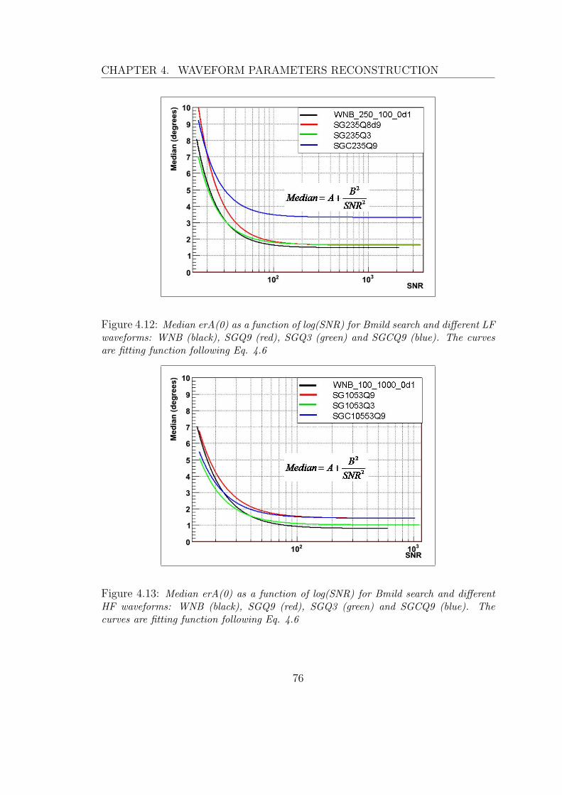
CHAPTER 4. WAVEFORM PARAMETERS RECONSTRUCTION
Figure 4.12: Median erA(0) as a function of log(SNR) for Bmild search and different LFwaveforms: WNB (black), SGQ9 (red), SGQ3 (green) and SGCQ9 (blue). The curvesare fitting function following Eq. 4.6
Figure 4.13: Median erA(0) as a function of log(SNR) for Bmild search and differentHF waveforms: WNB (black), SGQ9 (red), SGQ3 (green) and SGCQ9 (blue). Thecurves are fitting function following Eq. 4.6
76

4.4. RESULTS
Error Region
The introduction of Error Region is a useful trick to consider the reconstructionerrors due to algorithm approximations and the network geometry: its definitionis like an error area on reconstruction. However, the definition should satisfy twoconditions:
� well defined: the coverage of Error Region is corrected (Probability relatedto Error Region X is equal to X%, and not more or less);
� the Error Region is enough small (a few degrees).
These two conditions can be verified only with simulation tests.First of all we have to find a way to define Error Region for each reconstructed
events. We have just esplained before how we can do it: we convert the LikelihoodSky Map to a Probability Sky Map introducing a conversion function (Sec. 4.2.5).We can change the values of K and pr to change the performances. For wat-5.0.9tests the used values are:
� K0 = 10
� pr = 0.001
First of all we can compare the Error Region behaviour with Effective ErrorAngle using cumulative curves (Figs. 4.14 and 4.15). These figures report themedian value over all the directions of the Error Region (dashed curves) withrespect to the Effective Error Angle (continuous curves). A good definition ofError Region would make that the continuous and dashed curves cross at y-valueequal to 0.5, so that the Error Region cover the 50% of the injections direction.Moreover, if the corresponding value on x-axis is small (a few degrees) this makethe Error Region value usable. However, these conditions are quite satisfyed,because sometimes the Error Region is over estimated (the cross is over 0.5).
This fact could be accettable if the median behaviour is realized also for thesingle sky positions. In fact, the median value of Error Region reported in Fig.4.16 does not depend on the source directions. This means that the Error Region,if well defined, could be usable, because, even if the reconstruction is affected bythe network geometry, the Error Region does not care about it, so its performancesare general over the sky.
To verify if the Error Region is right defined, we must consider its coverage.This quantity is defined as the fraction of reconstructed events for which the ErrorRegion includes the injection position (i.e Error Region is bigger than Effective Er-ror Angle). If the coverage is equal to 50% of reconstructed events, Error Regionis well defined, otherwise it is under estimated (<50%) or over estimated (>50%).
77

CHAPTER 4. WAVEFORM PARAMETERS RECONSTRUCTION
Figure 4.14: Cumulative curves of Effective Error Angle (continuous) and Error Regiondashed) for WNB and SGQ9 LF waveforms. Bmild search is used for WNB, and Iweaksearch for SG. Brown line is equal to 50% of y-axis.
Figure 4.15: Cumulative curves of Effective Error Angle (continuous) and Error Regiondashed) for WNB and SGQ9 HF waveforms. Bmild search is used for WNB, and Iweaksearch for SG. Brown line is equal to 50% of y-axis.
78

4.4. RESULTS
Figure 4.16: Error Region for the 46 tested sky positions and WNB LF waveform, Bmildconstrain.
In Fig 4.17 we report the estimated coverage over the source directions. The figureshows that the quantity is strongly depending on the sky directions, which meansthat Error Region is not well defined over all the sky, but for some directions isunder estimated, and for others is over estimated.
Figure 4.17: Error Region coverage for the 46 tested sky positions and WNB LF wave-form, Bmild constrain.
In conclusion, Error Region definition does not satisfy all the desired goals,and so it is not usable. This carries out to two possibilities: try to improve theError Region definition to reach the desired goal, or leave behind this quantity
79

CHAPTER 4. WAVEFORM PARAMETERS RECONSTRUCTION
and implement an alternative option to substitute it. A probable solution is to useEffective Error Angle as a “frequentist” Error Region defined from simulations.However, this holds on the limitations which we described above: this quantity isnot general, because it is strongly dependent on the tested waveforms.
80

Chapter 5
LSC-Virgo Analysis
In this section we discuss the results of the first long term arch for GW burstsby the network of four detectors (V1, L1, H1, H2) belonging to Virgo and LSCcollaborations. The version of coherent WaveBurst used to analyze these data isnot as recent as the pipeline described in the previous section, which has beendeveloped after this analysis; in particular, the features of reconstruction of signalparameters were not comparable and the investigation of the accidental backgoundwas much more limited. However, this older version was already well performingfor what concerns the capability of identification of GW candidates and rejectionof accidental events, being the most advanced pipeline available at that time witha computational efficiency suitable for the analysis of a long term observation overa broad frequency bandwidth.
The search is targeted to GW bursts in the frequency range of 2 ÷ 6 kHz.We call this band High Frequency (HF) in opposition with the Low Frequency(LF), which considers frequencies lower than 2 kHz (Fig. 5.1). The cWB versionused for this work is the WAT 4.7.3 [101], adapted to run over a larger frequencyband than previously used. This has been the first coherent search in the HF bandand its responsibility was assigned to our Virgo group.
We describe in the following the data stream analysed (S5/VSR1), the MDCtested for the efficiency results and upper limits, the tuning procedure of the post-production thresholds and finally the results on zero lags.
5.1 Data set
The high sensitivity required for the GW detection implies that data are signifi-cantly affected by noise (Chapter 2.1). Interferometers are continuously checkedand commissioning work is regularly planned. When a particular test is performed,or the instrument is off to permit an hardware modification, the data stream is
81

CHAPTER 5. LSC-VIRGO ANALYSIS
Figure 5.1: Sensitivity curves for H1 (red), H2 (blue), L1 (green), V1(purple) duringJW1, a week joint period of data acquisition between Virgo and LSC. At 6 kHz the LSCdata show some sort of a ”cut-off” probably due to the calibration.
not usable for the detection of GWs. We use the word Science Mode to identifydata which can be used for GW detection.
A science run is a definite time period where the detector is in science mode.Start and stop run times are set to meet the scientific motivations decided for thatrun. This work uses the data stream belonging to the second year of the fifth LSCrun (S5Y2) and the whole first Virgo run (VSR1) according to the agreementbetween LSC and Virgo collaboration. We report in the Tab. 5.1 the starting andending times of these scientific runs.
RunStart Stop
GPS UTC GPS UTCS5Y2 847555214 2007-11-14 16:00:00 875289614 2007-10-01 16:00:00VSR1 863558950 2007-05-18 21:00:00 875253398 2007-10-01 05:56:24
Table 5.1: Start and stop in GPS and UTC times of the S5Y2 and VSR1 runs.
An subperiod of the S5Y2/VSR1 has been selected to perform pilot tests, the so
82

5.1. DATA SET
called JW1 (Joint Week 1, Tab. 5.2), about five days of coincidence time betweenthe four detectors (V1, H1, H2 and L1). In fact, this small period is representativeof the whole S5Y2/VSR1 for what concerns the detection efficiency. Therefore, itcan be used to compare the sensitivity of different settings of cWB parameters aswell as the robustness of cWB against calibration systematic errors with a limitedcomputational load perform mis-calibration tests, or to tune cWB parameters forthe analysis (this allows to decrease the computational load). Unfortunately, JW1background is not representative of the whole S5Y2/VSR1 period, so we cannotperform background tests on JW1 period and extend result considerations on thewhole S5Y2/VSR1, as for efficiency tests.
RunStart Stop
GPS UTC GPS UTCJW1 870052940 2007-08-02 01:22:06 870623383 2007-08-08 15:49:08
Table 5.2: Start and stop in GPS and UTC times of the JW1 period.
The data stream calibration to reconstruct h(t) is a remanding task, and itis very important for the correct use of a coherent data analysis to identify andestimate GW parameters. However, the calibration is not static, but revisions andadjustements produces new versions when possible. For this work we used the mostrecent calibration version available at the time of the analysis: the RDS C03 L2for LSC, the so called V3 [102], and the Hrec V2, also known as V2 [103] forVirgo. More details on the calibration are on the Sec. 5.1.2.
5.1.1 Data Quality
When a detector is in data taking mode, not all the data stream are consideredof good enough quality to be used for searching GW. The time list of data streamthat can be used for the analysis is provided by the Detector Characterizationand Data Quality Groups, according to the behaviour of the different detectorchannels. The various time lists referring to useful/not useful data stream can befound using the web interface provided by the group [104].
Lists can be collected in four main classes: Science Mode, Injection Mode,Locked Mode and Data Quality [105]. Each list is organised in segments, i.e. timeperiods of variable length which define the GPS times in which detector datastream are in good or bad quality. Start and stop times for each segment aredefined with 1 second resolution.
The informations stored for each list segments are:
� run tag (VSR1,...)
83

CHAPTER 5. LSC-VIRGO ANALYSIS
Figure 5.2: Definition of the segment’s boundaries. Starts and stops are respectivelyincluded and excluded from the segment.
� a progressive number (1, 2, 3)
� GPS start time
� GPS stop time
� state (-1, 0, 1)
where the state value is set according to Tab. 5.3
List type +1 0 -1Science Mode science mode not science mode not definedData Quality bad quality good quality not defined
Table 5.3: State definition for Science Mode and Data Quality segments. Not definedmeans that data have not yet been tested.
The output can be reported also in an ASCII file, in this case the list containsthe following values:
� segment number (1, 2, 3)
� GPS start time
� GPS stop time
� duration (optional)
84

5.1. DATA SET
We report now some informations on the different segment classes, focusing onVirgo detector.
Science Mode
Science Mode segments are the baseline lists for all data analysis. Segments belong-ing to this group are defined by the value of the Qc Moni ScienceMode channel,as recorded in the trend data frame files. This channel is derived online from theraw data, to be reliable and faster to read.
Definition of science mode is static (so there is no version number).
If the case of missing frame data or missing Qc Moni ScienceMode data, thescience mode status is defined as the last available status before interruption,except if the detector leaves science mode during the period of missing data.
In some cases, missing data segment could be long enough that the detectorcould leave and return to science mode during a single instance of missing data.In these cases the science status is manually double checked during the periods ofmissing data. If it is found that data are incorrectly marked as science mode, thisis handled by a specific data quality flag.
Injection Mode
This group identify time periods when simulated GW signals are physically injectedinto the detector. A flag (Alp Cali EVentInj STATUS) is produced and stored inthe raw data files. The missing data policy is similar to the one defined for thescience segment. The list of injections details (time, SNR, ...) are mantained inthe database indipendently of the segment list.
Locked Mode
This list corresponds to the time period when the detector is locked (see Sec.2.1). These segments could be useful for running online analysis in order tosupport commisioning activities. They could be interesting also to follow-upinteresting candidates identified by other detectors. The channel used is theAlp Main LOCK STEP STATUS. When this channel is set equal to 12, the flag inVirgo DataBase is set equal to 1, otherwise it set 0. If the channel is not available,the flag is set equal to −1. It is possible that for server problems the interfometeris not locked while Alp Main LOCK STEP STATUS=12. In this case a specificquality flag is produced to tag these time periods.
85

CHAPTER 5. LSC-VIRGO ANALYSIS
Data quality
The purpose of these segments is to identify periods of poor data quality or knownproblems that affect science mode segments. Some examples of data quality flagsare:
� incorrect science mode
� unmarked injections
� missing data
� bad h reconstruction
� airplane or helicopter overflight
� electrical power glitch
Data quality segments are used in conjunction with science mode segments torestrict the list of usable segments. These flags can be related to different thresh-olds (WIND OVER 40KPH, WIND OVER 50KPH) or different frequency bands(IBZ BRMS 60 300HZ, IBZ BRMS 600 700HZ), in this case they are imple-mented as separate flags. The newest version of a dataquality flag supercedesall previous versions and the database returns the most recent version unless auser explicitly requests an earlier version.
Data Quality flags are collected in several categories depending of the type ofusage and the characteristics (mainly efficiency and dead time):
� Category I: flag should be applied on data segments before event process-ing since we expect abnormal data characteristics that could jeopardize theperformances of the pipeline in adjacent periods.
� Category II: flag can be applied on the resulting triggers during the analysisor during the production stage. This category corresponds to well understoodmisfunctioning of the detector. The deadtime remains small (few %).
� Category III: flag should be applied to veto triggers after the analysis.It flags disturbances in environmental and instrumental auxiliary channelswhich are statistically correlated to excess noise and triggers on the gravita-tional wave channel, though their casual relation is not proved. Dead timemay be large and the interest of the DQ depends on the analysis. This cate-gory flag is used to select a subset of triggers with greater overall confidencesas GW candidates; however, any single trigger vetoed by a cat 3 cannot beconsidered a fake signal, given the statistical nature of the relationship with
86

5.1. DATA SET
disturbances. In fact, the use percentage, i.e. the fraction of Category IIIvetoes which succefully kill triggers in the GW channel, is low. This categorycould help in assessing an a posteriori confidence on plausibility for a GWcandidate.
We can include in this Category also the event by event vetoes [106]which are applied in the post-processing phase of the analysis. However,veto lists are different from DQ, in fact the start and stop times are notinteger numbers, but they reach the ms resolution. This because veto listsare constructed in different way and with the aim the select precisely definedtime periods which are particularly noising.
The same flag can be put in different categories for different analysis, howeverthere is a “recommended” category for each flag and standard analyses.
For this work we considered the Virgo VH2 [107] and the LIGO DQ 2.5[108]. Category I segments have been used to define the job segments, whereasCategory II have been used to define time periods during production analysis.
Data Quality flags are set separately for each considered detector, their in-tersection define the livetime of network configurations made by different sets ofdetectors. In the Tab. 5.4 we report the exclusive1 live times for all the possiblenetwork configurations considering the four detectors after applying the LSC andVirgo DQ Category II.
We have decided to analyses network configurations with sufficient duty time(in red in the Tab. 5.4), including the H1L1V1 network, for the possibility forthis configuration to increase statistic adding a fixed shift on the second detector(Section 5.3.2).
5.1.2 Calibration Issues
The reconstructed h(t) data stream is affected by a frequency dependence cali-bration uncertainty for the amplitude and phase (or time offset). The amplitudeuncertainty is reported as estimated deviation plus its one sigma estimate. In fact,different calibration measurements show that the mis-calibration in amplitude ofeach detector apparently fluctuates from time to time in a random way. It is notknown how much of these fluctuations are due to the actuators which force themirrors to inject reference signals during the calibration measurements or insteadto a true change in calibration of the GW sensing of the interferometer.
1The H1H2L1V1 concidence period is inside the H1H2L1 one. The H1H2L1 esclusive time isdefined as the entire H1H2L1 coincidence time excluding the H1H2L1V1 time. Same definitionis applied for the other networks.
87

CHAPTER 5. LSC-VIRGO ANALYSIS
Number of Network Live timedetectors [days]
4 H1 H2 L1 V1 68.9
3
H1 H2 L1 124.5H1 H2 V1 15.8H1 L1 V1 4.5H2 L1 V1 1.3
2
H1 H2 35.4H1 L1 7.2H2 L1 3.8H1 V1 1.8H2 V1 0.8L1 V1 6.3
Table 5.4: Exclusive live times for all network configurations during S5Y2/VSR1 period.In red the network that have been analysed for this work.
These fluctutations of amplitude calibration should than be considered becausethey may affect the estimation of the efficiency and upper limits. To consider thisfact simulation tests are made injecting “ad-hoc” simulated signals. In practicewe mimic the effect of calibration systematics on the detection eficiency of thenetwork by injecting sotware GW signals with uncalibrated amplitude and phasecharcteristics in different detectors (Sec. 5.4). In this work we considered twoeffects:
� the use of not final calibration versions. In fact, when we started the analysis,the LSC V4 and Virgo V2 calibrations were not ready. Luckily, the Virgo V2was ready in time to re-run the analysis, but for LIGO detectors we had tostick to the V3 calibration and then take into account the known systematicsbetween V3 and V4 calibration [109] as a sistematic uncertainty on the V3.
� the rated uncertainties of the final calibration versions. Virgo reports asimple upper limit on the expected amplitude and phase/time calibrationsystematics. LIGO reports the rms taken from the calibration measurements.
The systematic errors expected for Virgo V2 [103] are:
� amplitude: 6%
� time: 6µs above 1.9 kHz
These are meant as upper limits, but to be conservative we considered them asstandard deviations.
88
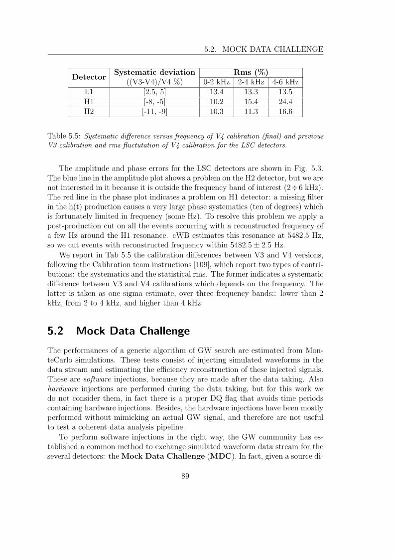
5.2. MOCK DATA CHALLENGE
DetectorSystematic deviation Rms (%)
((V3-V4)/V4 %) 0-2 kHz 2-4 kHz 4-6 kHzL1 [2.5, 5] 13.4 13.3 13.5H1 [-8, -5] 10.2 15.4 24.4H2 [-11, -9] 10.3 11.3 16.6
Table 5.5: Systematic difference versus frequency of V4 calibration (final) and previousV3 calibration and rms fluctutation of V4 calibration for the LSC detectors.
The amplitude and phase errors for the LSC detectors are shown in Fig. 5.3.The blue line in the amplitude plot shows a problem on the H2 detector, but we arenot interested in it because it is outside the frequency band of interest (2÷6 kHz).The red line in the phase plot indicates a problem on H1 detector: a missing filterin the h(t) production causes a very large phase systematics (ten of degrees) whichis fortunately limited in frequency (some Hz). To resolve this problem we apply apost-production cut on all the events occurring with a reconstructed frequency ofa few Hz around the H1 resonance. cWB estimates this resonance at 5482.5 Hz,so we cut events with reconstructed frequency within 5482.5± 2.5 Hz.
We report in Tab 5.5 the calibration differences between V3 and V4 versions,following the Calibration team instructions [109], which report two types of contri-butions: the systematics and the statistical rms. The former indicates a systematicdifference between V3 and V4 calibrations which depends on the frequency. Thelatter is taken as one sigma estimate, over three frequency bands:: lower than 2kHz, from 2 to 4 kHz, and higher than 4 kHz.
5.2 Mock Data Challenge
The performances of a generic algorithm of GW search are estimated from Mon-teCarlo simulations. These tests consist of injecting simulated waveforms in thedata stream and estimating the efficiency reconstruction of these injected signals.These are software injections, because they are made after the data taking. Alsohardware injections are performed during the data taking, but for this work wedo not consider them, in fact there is a proper DQ flag that avoids time periodscontaining hardware injections. Besides, the hardware injections have been mostlyperformed without mimicking an actual GW signal, and therefore are not usefulto test a coherent data analysis pipeline.
To perform software injections in the right way, the GW community has es-tablished a common method to exchange simulated waveform data stream for theseveral detectors: the Mock Data Challenge (MDC). In fact, given a source di-
89

CHAPTER 5. LSC-VIRGO ANALYSIS
Figure 5.3: Amplitude and phase systematics as a function of frequency for the threeLSC detectors. Blue line in amplitude shows a problem on the H2 detector. Phase errorshown in red at 5.5 kHz for H1 indicates a problem with the filters used in the h(t)production.
rection in the sky, the wavefron will hit the detectors at different times. Morevoer,each detector senses a different combination of + and × polarizations, due to thedifferent orientations of the detector’s arms (Eq. 2.3). The MDC data streamcontains a set of gravitational waveforms to be added in each detector data streamlisting the following parameters:
� the source direction
� time arrival at each detector, and at the earth center
90

5.2. MOCK DATA CHALLENGE
� h+ and h× polarization waveforms at earth
� F+ and F× directional sensitivity components for each detector
� hrss values at the earth
MDC are produced by a software developed in the LIGO group: the Burst-MDC package [110].
We cannot test the pipeline over all possible GW Burst Waveforms nor we canprovide any “complete” set of waveforms.
We have produced two sets, which we have identified with the label SGQ9 andMDC2 and we explained in details in the following sections.
5.2.1 Sine Gaussian MDC set
This set is composed of Sine Gaussian waveforms. The general formula of a SineGaussian is:
h = e−(t/τ)2Sin(2πft) (5.1)
where the decay time depends on central frequency f : τ = Q√2πf
. So usually the
set is identified with the value of Q chosen.SineGaussians have been chosen because thay are compact signals in the time-
frequency plane. Moreover, by varying the central frequency and Q value, theycan probe systematically a reasonable large burst parameter space.
For our test we use the HSG7 S5 R3 version [111], with the following char-acteristics:
� 13 central frequencies, approximately equally spaced in logarithmic frequencyin the HF band (Tab. 5.6 and Fig. 5.4). The choice of frequency was fixedin a previous analysis.
� Q=9, if f ≈ 1415÷ 6000 Hz, τ ≈ 0.34÷ 1.43 ms.
� Reference strength: hrss=2.5 · 10−21 1/√Hz.
� Injections every 100 s, injection time randomly chosen within± 10 s of center.
� Random selection of the 13 waveforms at each injection time, so that themean rate of each waveform is 1/1300 s.
� Input waves are linearly polarized signals.
� Simulation randomly selects sky directions from a uniform distribution in thesky and polarization angle from a uniform distribution in [0, ψ], thereforegetting a random combination of h+ and h× polarizations at earth.
91

CHAPTER 5. LSC-VIRGO ANALYSIS
We distinguish each waveform indicating the central frequency and the Q. So,a generic SineGaussian is named SGXXXXQY, where X is the central frequency,and Y the Q.
SGQ9SG1415Q9 SG1615Q9 SG1797Q9 SG2000Q9 SG2226Q9SG2477Q9 SG2756Q9 SG3067Q9 SG3413Q9 SG3799Q9SG4225Q9 SG5000Q9 SG6000Q9
Table 5.6: List of waveforms belonging to SGQ9 set.
Figure 5.4: Fourier Transform of SGQ9 set. Frequencies are spaced according to thebandwidths of the waveforms.
This set has been used to tune the post-production parameters of the cWB forthe several network configurations (Chapter 5.3.4).
5.2.2 Second MDC set
It is preferable to test the pipeline also on other waveforms with different time-frequency characteristics, to mimic a larger fraction of possible astrophysical pro-
92

5.2. MOCK DATA CHALLENGE
cesses. For this purpose we have prepared a second MDC set, which contains thefollowing waveform:
� Sine Gaussian (SG) wih shorter and longer duration;
� White Noise Bursts (WNB);
� Ring Downs (RD);
� Numerical Supernova Waveforms (SN).
We planned to use a unique set including these waveforms to reduce the compu-tational load, mantaining a sufficient statistic to obtain reliable efficiency curves.However, some technical problems with BurstMDC force us to divide the wave-forms in two separate sets (HBRST1 and HBRST2), so we decide to halve theinjection rate of signals (1 every 200 s instead of 100 s) to mantain the plannedcomputational load. Other characteristics are the same for the SGQ9 set. In theTab. 5.7 there is the list of waveforms for the two sets.
HBRST1
RD
RDL 200 1590 RDL 200 2090 RDL 200 2590RDC 200 1590 RDC 200 2090 RDC 200 2590RDL Q9 2000 RDL Q9 3067 RDL Q9 5000RDC Q9 2000 RDC Q9 3067 RDC Q9 5000
WNBWNB 2000 1000 0d01 WNB 3500 1000 0d01 WNB 5000 1000 0d01WNB 2000 100 0d1 WNB 2500 100 0d1 WNB 5000 100 0d1
HBRST2
SGSG1615Q3 SG2000Q3 SG2477Q3 SG3067Q3 SG5000Q3
SG1615Q100 SG2000Q100 SG2477Q100 SG3067Q100 SG5000Q100SN D1 D4
Table 5.7: List waveforms belonging to MDC2 set.
Sine Gaussians
The name convention for the SineGaussian are the same as the SGQ9 set. Inthis set we use waveforms with different Q: 3 and 100. In the range centralfrequency 1415 ÷ 6000 we obtain decay times for Q=3 (100) between 0.11 ÷ 0.47(3.75 ÷ 15.90) ms. These waveforms are used to test the pipeline on differentduration and bandwidth scales with respect to SGQ9.
93

CHAPTER 5. LSC-VIRGO ANALYSIS
White Noise Bursts
These waveforms are Bursts built by bandpassing in a selected bandwidth a whitenoise of selected duration with independent polarization amplitudes. These areconsidered as the limiting case signals, since they have a close resemblance tothe noise of each detector and stand up in the network data analysis just be-cause they partially correlate the detector responses. The name convention is:WNB startfreq bandwidth duration. Each waveform type is made by a pair ofrandom h+ and indipendent random h×. This is accomplished bt sampling ran-domly the h+ and h× waveforms from a set of 30 scalar waveforms, thereforeobtaining 30x29 independent h+/× couples.
Ring Down
Ring Down waveform are expected from processes like f-modes of NS, or during theRing-Down of newly formed BH/NS during the post merger phase after coalesce(Chapter 1.2.1), or produced in SN star-quakes related to Soft Gamma Repeaters(SGR). They are characterized by frequency, τ or Q (similarly to SG) and polar-ization. The name convention is: RD* tau frequency or RD* Q frequency, wherethe * indicates the polarization: “L” stands for linear polarization (h× = 0) and“C” for circular polarization.
The expression for Ring Down waveform with circular polarization is:(h+
h×
)=hrssπfτ
√1 + 4π2f 2τ 2
τ(1 + e−1/(2fτ))e−t/τ
(Cos2ψ −Sin2ψSin2ψ Cos2ψ
) (1+cos2ι
2Θ(t− 1
4f)Cos(2πft)
Cos(ι)Θ(t)Sin(2πft)
)(5.2)
where we have defined:
h2rss =
∫ ∞
0
(|h+(t)|2 + |h×(t)|2)dt (5.3)
the angle ψ is an arbitrary GW polarization uniformly distribuited in [0, π] andthe angle ι an arbitrary inclination of the system wich originates the burst withrespect to the line of sight. If we assume a random orientation in space of the axisof symmetry of the emitting system the cos(ι) should be uniformly distribuitedin [-1, 1]. The Θ function is introduced to avoid a discontinuity at the beginningof the waveform which would result into a infinite energy. Linearly polarized RDconsider only the h+ component in the expression above
SN waveforms
These waveforms are predicted from processes of SN core collapse. We have con-sidered two waveforms among the great variety in literature, which we indicate
94

5.2. MOCK DATA CHALLENGE
with the name D1 and D4 [112]. The first is generated by the collapse of a 1.26solar mass star that is almost spherical at the time of the transition into a BH,while the latter is generated by the collapse of a 1.86 solar mass star that is max-imally deformed at the time of the transition into a BH. Only the h+ componentis considered, because the h× is smaller by more than an order of magnitude (Fig.5.5).
Figure 5.5: D1 (up) and D4 (down) waveforms in time domain, plus (left) and cross(right) components. The possible sources are at a distance of 10 kpc.
All the waveforms are generated with a reference amplitude hrss = 2.5 · 10−21
Hz−1/2 except for the SN. In this case the signal amplitude is set by the numericalsimulations of the source, so that changing the injected hrss at earth is equivalent
95
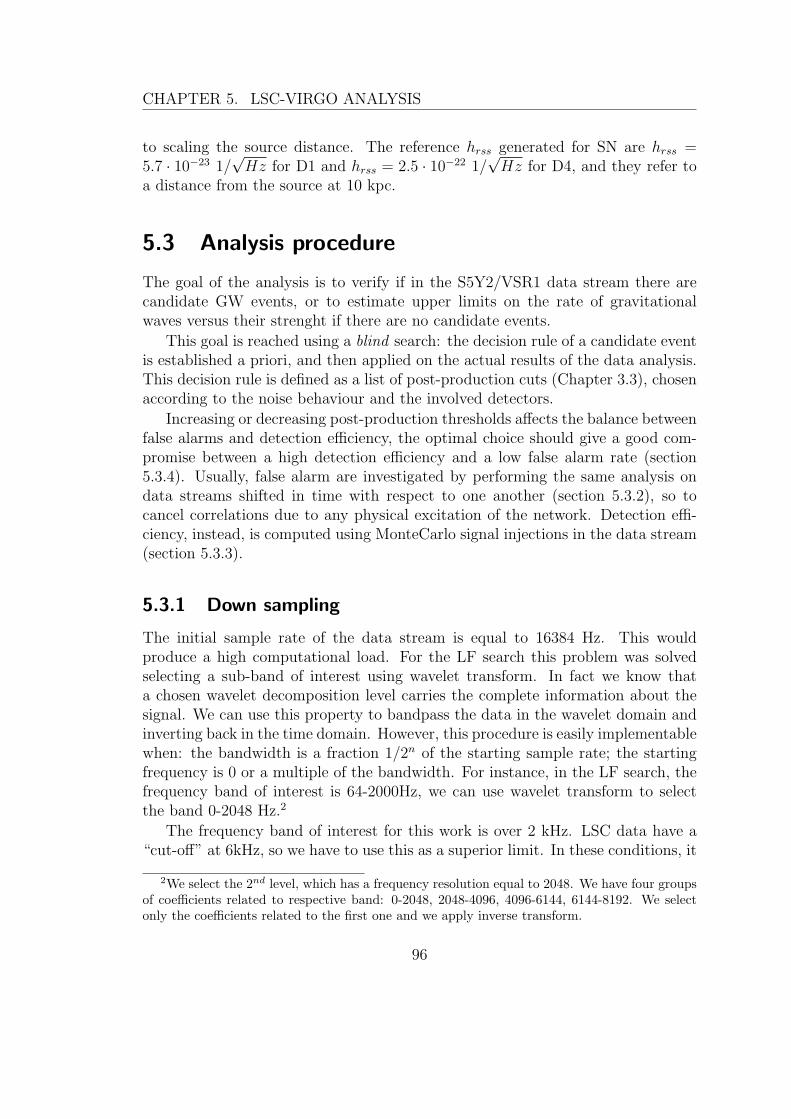
CHAPTER 5. LSC-VIRGO ANALYSIS
to scaling the source distance. The reference hrss generated for SN are hrss =5.7 · 10−23 1/
√Hz for D1 and hrss = 2.5 · 10−22 1/
√Hz for D4, and they refer to
a distance from the source at 10 kpc.
5.3 Analysis procedure
The goal of the analysis is to verify if in the S5Y2/VSR1 data stream there arecandidate GW events, or to estimate upper limits on the rate of gravitationalwaves versus their strenght if there are no candidate events.
This goal is reached using a blind search: the decision rule of a candidate eventis established a priori, and then applied on the actual results of the data analysis.This decision rule is defined as a list of post-production cuts (Chapter 3.3), chosenaccording to the noise behaviour and the involved detectors.
Increasing or decreasing post-production thresholds affects the balance betweenfalse alarms and detection efficiency, the optimal choice should give a good com-promise between a high detection efficiency and a low false alarm rate (section5.3.4). Usually, false alarm are investigated by performing the same analysis ondata streams shifted in time with respect to one another (section 5.3.2), so tocancel correlations due to any physical excitation of the network. Detection effi-ciency, instead, is computed using MonteCarlo signal injections in the data stream(section 5.3.3).
5.3.1 Down sampling
The initial sample rate of the data stream is equal to 16384 Hz. This wouldproduce a high computational load. For the LF search this problem was solvedselecting a sub-band of interest using wavelet transform. In fact we know thata chosen wavelet decomposition level carries the complete information about thesignal. We can use this property to bandpass the data in the wavelet domain andinverting back in the time domain. However, this procedure is easily implementablewhen: the bandwidth is a fraction 1/2n of the starting sample rate; the startingfrequency is 0 or a multiple of the bandwidth. For instance, in the LF search, thefrequency band of interest is 64-2000Hz, we can use wavelet transform to selectthe band 0-2048 Hz.2
The frequency band of interest for this work is over 2 kHz. LSC data have a“cut-off” at 6kHz, so we have to use this as a superior limit. In these conditions, it
2We select the 2nd level, which has a frequency resolution equal to 2048. We have four groupsof coefficients related to respective band: 0-2048, 2048-4096, 4096-6144, 6144-8192. We selectonly the coefficients related to the first one and we apply inverse transform.
96
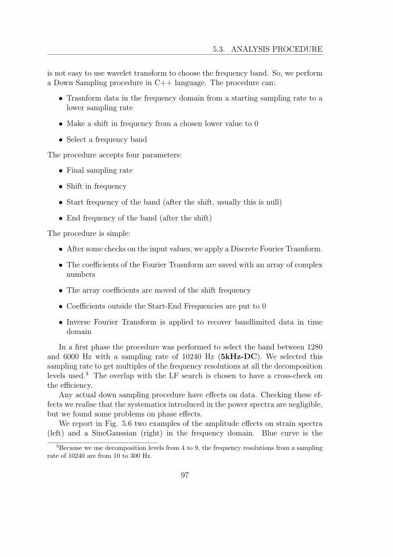
5.3. ANALYSIS PROCEDURE
is not easy to use wavelet transform to choose the frequency band. So, we performa Down Sampling procedure in C++ language. The procedure can:
� Trasnform data in the frequency domain from a starting sampling rate to alower sampling rate
� Make a shift in frequency from a chosen lower value to 0
� Select a frequency band
The procedure accepts four parameters:
� Final sampling rate
� Shift in frequency
� Start frequency of the band (after the shift, usually this is null)
� End frequency of the band (after the shift)
The procedure is simple:
� After some checks on the input values, we apply a Discrete Fourier Trasnform.
� The coefficients of the Fourier Trasnform are saved with an array of complexnumbers
� The array coefficients are moved of the shift frequency
� Coefficients outside the Start-End Frequencies are put to 0
� Inverse Fourier Transform is applied to recover bandlimited data in timedomain
In a first phase the procedure was performed to select the band between 1280and 6000 Hz with a sampling rate of 10240 Hz (5kHz-DC). We selected thissampling rate to get multiples of the frequency resolutions at all the decompositionlevels used.3 The overlap with the LF search is chosen to have a cross-check onthe efficiency.
Any actual down sampling procedure have effects on data. Checking these ef-fects we realise that the systematics introduced in the power spectra are negligible,but we found some problems on phase effects.
We report in Fig. 5.6 two examples of the amplitude effects on strain spectra(left) and a SineGaussian (right) in the frequency domain. Blue curve is the
3Because we use decomposition levels from 4 to 9, the frequency resolutions from a samplingrate of 10240 are from 10 to 300 Hz.
97

CHAPTER 5. LSC-VIRGO ANALYSIS
Figure 5.6: Effect of 5kHz-DC on amplitude for Virgo spectra (left) and SG3067Q9(right). Blue curve is the amplitude of original data (16384 Hz) applying a Blackman-Harris window, the black curve represents the differences between FFT converted to thesample rate of 10240 Hz and the original one (16384 Hz).
original amplitude applying a Blackman-Harris window, the black curve representsthe differences between FFT converted to the sample rate of 10240 Hz and theoriginal one. Effects are small by orders of magnitude.
Unfortunately, the Down Conversion has a great distortion on the carrier part,whose frequency is shifted by the value of the start frequency. For instance, aSineGaussian with initial central frequency equal to 2000 Hz is down converted toa central frequency of 720 Hz (2000-1280). This is not a big problem, because thesignal envelope is preserved, the waveform mantains the same duration and thearrival time does not change in a significant way. The problem is that the signalshape is modified depending on the phase of arrival of its carrier with respect to thereference frequency of the down-sampling (1280 Hz). If the SineGaussian phaseis incoming π/2 later with respect to the 1280 Hz reference, the down convertedsignal becomes a CosineGaussian (Fig. 5.7).
We cannot neglect this effect because cWB considers the signal shape to makecoeherent considerations and reconstruct the waveform. In practice, the recon-struction of the signal characteristics, e.g. the source direction and signal wave-forms, turns out to be severely jeopardized and the resulting sensitivity gets worse,typically requiring signal amplitudes greater by 10% to get the same detection effi-ciency with respect to the analysis without downsampling. To avoid this problemwe had to eliminate the frequency shift, and we chose a final sample rate of 12800Hz, selecting all the band between 0-6400 Hz. The choice of frequency band of1280-6000 Hz is made using cWB selections in the wavelet domain. The samplerate of 12800 Hz has been chosen making the same considerations about frequencyresolutions of the decomposition levels. Using this sample rate, and decompositionlevels from 4 to 9, we obtain a frequency resolution from 12.5 to 400 Hz (and a
98
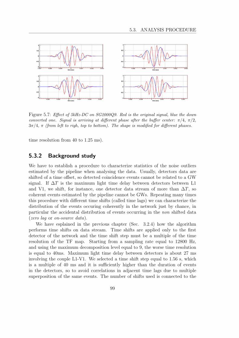
5.3. ANALYSIS PROCEDURE
Figure 5.7: Effect of 5kHz-DC on SG2000Q9. Red is the original signal, blue the downconverted one. Signal is arriving at different phase after the buffer center: π/4, π/2,3π/4, π (from left to righ, top to bottom). The shape is modified for different phases.
time resolution from 40 to 1.25 ms).
5.3.2 Background study
We have to establish a procedure to characterize statistics of the noise outliersestimated by the pipeline when analysing the data. Usually, detectors data areshifted of a time offset, so detected coincidence events cannot be related to a GWsignal. If ∆T is the maximum light time delay between detectors between L1and V1, we shift, for instance, one detector data stream of more than ∆T , socoherent events estimated by the pipeline cannot be GWs. Repeating many timesthis procedure with different time shifts (called time lags) we can characterize thedistribution of the events occuring coherently in the network just by chance, inparticular the accidental distribution of events occurring in the non shifted data(zero lag or on-source data).
We have esplained in the previous chapter (Sec. 3.2.4) how the algorithmperforms time shifts on data stream. Time shifts are applied only to the firstdetector of the network and the time shift step must be a multiple of the timeresolution of the TF map. Starting from a sampling rate equal to 12800 Hz,and using the maximum decomposition level equal to 9, the worse time resolutionis equal to 40ms. Maximum light time delay between detectors is about 27 msinvolving the couple L1-V1. We selected a time shift step equal to 1.56 s, whichis a multiple of 40 ms and it is sufficiently higher than the duration of eventsin the detectors, so to avoid correlations in adjacent time lags due to multiplesuperposition of the same events. The number of shifts used is connected to the
99

CHAPTER 5. LSC-VIRGO ANALYSIS
maximum time shift we can apply to data, i.e. 300 s, which is the minimum lengthof a job segments. In fact, as discussed in Chapter 3.2.4, the reference detector isshifted circularly within the segment and a shift equal to segment duration wouldjust be equivalent to the zero lag. According to these considerations, maximumlag number used is 192 (192 · 1.56 < 300 < 193 · 1.56). In case a larger statistics isneeded to investigate the distribution of accidental triggers, when three or moresites are involved we can repeat the time slides on the same reference detectorapplying a fixed time offset to another site. We used this possibility for the V1H1L1network: also the H1 detector has been shifted by a time of 1.56 s and 3.12 s. Inthis way we obtain three indipendent analyses composed of 192 lags each and wetriplicate the livetime.
In the following considerations we indicate reference detector as the first in thename of each configuration. For instance, the reference detector for the networkV1H1H2L1 is V1, for L1H1H2 is L1, and so on. We have not a complete freedomfor the choice of reference detector: co-located detectors show a foreground noisemade by correlated local disturbances, so they should not be shifted one with re-spect to the other. In fact, the existing foreground noise of H1 and H2 is a sourceof accidental triggers for the network configurations which include that pair ofdetectors, and shifting H1 with respect to H2 would eliminate this contribution.Another consequence of the H1H2 foreground noise is that time lag analysis can-not be used to measure the false alarm probability of H1H2 on-source candidates.Therefore, since we are lacking a robust estimate of its accidental background dis-tribution, the H1H2 configuration has been analyzed only for setting a conservativeupper limit on the GWs.
Background analyses have been used to tune the analysis thresholds. We decideto divide the background events list in two equal parts: the one belonging to theodd lags and the other belonging to the even. Only the first list has been used totune the post production cuts (tuning set) at a chosen false alarm rate, while thesecond has been kept undisclosed until the tuning was frozen (estimation set).Then we apply post production cuts to the second set to estimate the actual falsealarm rate of set by the chosen thresholds as well as the false alarm rate of anyfound candidate for each network configuration. In this way we avoid the risk ofbiding the false alarm estimate and can also verify the consistency between oddand even lags regarding the false alarm estimation.
For network configurations involving both V1 and L1, we decided to shift V1.This choice was made according to preliminary tests on JW1 period, which showa better efficiency at the same post-production thresholds when V1 is used a refer-ence detector. This is related to the asymmetric location of the detectors involvedin the network. Light travel time between detectors is almost equal consideringthe couples V1-L1 and V1-H1 (about 27 and 24 ms), while between Hanford and
100

5.3. ANALYSIS PROCEDURE
Livingston it is significantly shorter (about 10 ms). The algorithm computes thelikelihood over the sky in the time reference of the first detector, i.e. the data ofthe other detectors gets shifted by the light travel time corresponding to a grid ofsky directions (App. A.1). When choosing V1 as a reference detector the pipelinereconstructs sky directions using time delays bounded within ± 27 and 24 ms, in-stead if we choose L1, one of the maximum time delays is significant smaller. Thechoice of V1 as reference detector then gives more possibilities to the algorithmto look for coherent signals, so that in the ideal case one would expect a higheraccidental background and the same detection efficiency for real GW signals. Itturns out, however, that this is not the case and that it is convenient to keep V1 asreference, since the background increase is negligible and instead the measured de-tection efficiency gets improved, as demonstrated in tests on the JW1 period. Thisis likely due to the approximations used within the algorithm to find candidatecoherent signals.
Tuning procedures for all the network configurations (included H1H2, which isslightly different from the others) are explained in the Chapter 5.3.4.
Figure 5.8: Background behaviour of V1H1H2L1: ρ versus frequency (left) and rateversus lag (right). In this test, the post-production thresholds are set low enough tostudy also the background at low SNRs. The frequency dependence shows that accidentalevents are not white, but instead occur in frequency bands related to disturbances atdifferent detectors. The overal count of accidental event per lag are however Poissondistributed and do not show a dependence on the time shift.
5.3.3 Efficiency study
Detection efficiency depends on multiple factors: signal injection hrss, frequency,waveform, pipeline, in particular on the post production thresholds. We have justesplained the reasons on the choice to test cWB on SGQ9 set (Chapter 5.2.1). This
101

CHAPTER 5. LSC-VIRGO ANALYSIS
set is produced with a fixed hrss equal to 2.5 · 10−21 1/√Hz. To test a wide range
of signal amplitudes, cWB uses a grid of factors to scale the reference amplitudeand repeat the software signal injections of the same MDC set. In this way, weconstruct an efficiency curve for each waveform, i.e. a plot showing the efficiencyvalue as a function of injected hrss (or amplitude scaling factor). The range ofthese scaling fatcors should cover the entire detection efficiency curve, from near0% to near 100% efficiency per each waveform.
We have chosen 18 amplitude factors, logaritmically spaced which allow thisinvestigation for almost all tested waveforms (Fig. 5.9).
Figure 5.9: Efficiency curves for SGQ9 set, V1H1H2L1 network, JW1 period. This is atest, post-production thresholds correspond to a higher false alarm rate with respect whatis required for a GW search.
From efficiency curves, we fit the values of injected hrss correponding to the10%, 50% and 90% of efficiency and we consider these values as figure of meritsamong different waveforms or searches.
Efficiency curves also guide the astrophysical implementation of the searchresults.
5.3.4 Thresholds tuning
The main goal of the tuning procedure is to select events making a balance betweenthe probability of false alarm and the detection efficiency.
102

5.3. ANALYSIS PROCEDURE
The adopted tuning procedure is the following:
� target a false alarm rate suitable for foreground investigations and for settingupper limits, which is approximately 5 · 10−9 1/s (∼1 over 6 years);
� select post production thresholds so to maximize the detection efficiency forSGQ9 keeping approximately constant the target FAR;
� estimate the false alarm rate of events passing the threshold of previousstep by a procedure defined a priori, which ranks the significance of selectedevents as a function of their ρ. The number of time lags will be increased asneeded to ensure the statistical uncertatinty on FA.
We remind here the post production thresholds (Chapter 3.3):
� Penalty: p > pth
� Effective Correlated SNR: ρ > ρth
� Network Correlation Coefficient: cc > ccth
in addition we have added a frequency cut on networks involving H1 to consideronly events with central frequency outside the band [5482.5 - 2.5, 5482.5 + 2.5] Hzfor calibration problems on H1 (Chapter 5.1.2). Events which satisfy the condition|f − 5482.5Hz| > 2.5 Hz pass this cut (f is the estimated central frequency).
We remind that penalty cut (Sec 3.3.1) is is defined as the square root ofthe fraction between the total energy in the detector and the reconstructed energyresponse and it is used to avoid unphysical solutions when energy response isgreater than total energy in the detector data stream. This is a general conditionand it is not necessary to tune it for the different networks, so we decide to adoptthe threshold used in the LF frequency, which has been previously tested in theLF band. We do not expect relevant differences regarding this cut. The pth is setequal to 0.6 for all networks.
The other two thresholds, instead, have to be tuned depending on the per-formances of the detector configurations. Results performances gets better whenthe number of detectors involved is higher, because the network gives more infor-mation to the pipeline. We cannot use the same post production cuts of the LFsearch, because noise behaviour between detectors on HF is different from LF.
We adopt a common procedure to choose the values of ρth and ccth for eachconfiguration, and we apply this procedure on tuning set (odd lag) and SGQ9simulations.
First we consider the ρ versus cc distribution of background and SGQ9 events(Fig. 5.10). From this plot we select some convenient cc thresholds (usually
103

CHAPTER 5. LSC-VIRGO ANALYSIS
4 thresholds with a coarse step of 0.5) which can separate the populations ofreconstructed injections and of accidental triggers. Referring to Fig. 5.10, ccthtoo near to unity would eliminate too many SGQ9 events, otherwise for very lowvalues of ccth too many background events would pass.
Figure 5.10: Distribution of ρ and cc values for background (black) and SGQ9(coloured) events for V1H1H2L1 network. Coloured lines show candidate thresholds oncc: black→0.5, red→0.55, green→0.6, blue→0.65.
For each value of cc thresholds chosen we produce the accidental event rateversus ρ (Fig. 5.11) and we find the corresponding ρth ensuring the target falsealarm rate.
We compare the resulting hrss 90% detection efficiencies of these different [ρ,cc] settings for the SGQ9 set (Fig. 5.12) and select the one that performs best inthe band 2-6 kHz.
Final thresholds are selected automatically using an implemented procedure.This ranking procedure scores more the lowest hrss 90%. It considers the couples[ρi, cci] for each network i. Then, for each SGQ9 frequency, we have hrss 90%values corresponding to each couple: hrss90%[1] and hrss90%[2]. The procedureassigns a score to the couple [ρi, cci] that at each frequency beats by at least 10%the hrss90% of the others. After calculating the scores for each [ρi, cci] couple, theprocedure selects the couple with higher score. If two or more couples have thesame score, the procedure choose the one with lowest cc value.
For the V1H1L1 network a difference between tuning and estimation sets of
104

5.3. ANALYSIS PROCEDURE
Figure 5.11: Accidental event rate versus ρ for V1H1H2L1 network. The red line showsthe target false alarm rate of ∼1/6 years.
Figure 5.12: Hrss 10-50-90% efficiency for SGQ9, V1H1H2L1 network, per each pairof (ρ, cc) thresholds which match the target false alarm rate.
the background forced us to set more conservative thresholds with the respect tothe automatic procedure. This is described in section 5.5.2.
Final thresholds for all configurations are on Tab. 5.8
105

CHAPTER 5. LSC-VIRGO ANALYSIS
Network pth ccth ρth
V1H1H2L1 0.6 0.6 4.3L1H1H2 0.6 0.6 4.1V1H1H2 0.6 0.7 4.6V1H1L1 0.6 0.6 6.0H1H2 0.6 0.5 5.0
Table 5.8: Final values of pth, ρth and ccth for the different network configurations.
H1H2 Tuning
The tuning of H1H2 configuration cannot be performed in the same way as theother configurations. This is due to the fact that we cannot characterize H1H2background with time lags between the two detectors, as we have previously de-cided. We decide to make statistical analysis on H1H2 configuration with the goalto compute upper limits on GW, so the tuning procedure is slightly different: giventhe unknown foreground systematics, we select more conservative thresholds withrespect to the accidental event distribution obtained from time lags.
We decide to characterize background with different H1H2 analyses:
� zero lag playground: zero lag analysis on time periods corresponding toV1H1H2L1, L1H1H2 and V1H1H2 network observative time (approximative208 days). Since a null results has been achieved for these configurations,this is almost an off-source sample for GWs. We are not assured of a nullresult for H1H2, but it is very likely.
� off-source playground: 192 lag analysis on time periods corresponding toV1H1H2L1, L1H1H2 and V1H1H2 network observative time. This is an off-source sample, but any foreground noise due to correlated H1H2 responsesis canceled as well
� off-source background: 192 time lags on the H1H2 exclusive live time.
We select final thresholds in the following way. Looking at the scatter plotof accidental events and MDC SGQ9 injections (Fig. 5.13), we fix a priori thecc threshold equal to 0.5. In fact, the ρ threhold is set extrapolating above theloudest event among the three analysis considered (off-source background, Fig.5.14). We consider both the odd and even lags (no separation between tuning andestimation set) for each of the three analysis to have more statistics, in fact thenumber of background events is very small, respect to the other configurations ofdetectors (Figs. 5.12 and 5.13). This is due to the fact that they are colocated,so that the expected coherent response in the two detectors is so well constrained
106

5.4. EFFECTS OF CALIBRATION SYSTEMATICS ON RESULTS
that makes much less likely for accidental triggers and for foreground triggers topass the coherent analysis and conseguently the reconstructed background eventsare reduced.
Figure 5.13: Distribution of ρ and cc values for background (black) and SGQ9 (coloured)events for H1H2 network. Off-source background on left and off-source playground onright.
Comparing SGQ9 efficiency results for different ρ thresholds (Fig. 5.15) werealize that the choice of ρth can be conservative, without paying too much on theefficiency side. The loss in efficiency is very small increasing ρ threshold from 4 to5, so we can choose the most conservative value, i.e. above the loudest event, forour goal. So the chosen ρth is equal to 5.0.
5.4 Effects of Calibration Systematics on results
To test the robustness of our detection efficiency results with respect to calibrationsystematic uncertainties, we performed MonteCarlo software injections using adhoc mis-calibrated signals. The difference in hrss 50% between calibrated and mis-calibrated data can be used as an error of the efficiency estimate due to calibrationuncertainties.
The pipeline has been sligthly modified to perform mis-calibration tests. Foramplitude/phase mis-calibrations, before injecting MDC waveforms in the datastream, we modify on the fly their amplitudes/phases according to the availableestimate of calibration systematics. Usually we indicate applied mis-calibrations
107

CHAPTER 5. LSC-VIRGO ANALYSIS
Figure 5.14: Accidental event rate versus ρ for H1H2 network and off-source background(black), off-source playground (red), zero lag playground (green). Zero lag playground hasa very poor statistics but anyway does not contradict the other estimated. The off-sourceplayground and background are in agreement in the tail and the former corresponds to amuch longer livetime and therefore can investigate lower False Alarm Rates.
Figure 5.15: Hrss 10-50-90% efficiency for SGQ9, H1H2 network, obtained using dif-ferent ρ thresholds and the same cc.
with the relative fraction respect to the original amplitude or with the equivalentnumber of samples for the phase.
As a matter of fact, phase shifts are technically implemented by delaying or
108

5.4. EFFECTS OF CALIBRATION SYSTEMATICS ON RESULTS
anticipating the waveform by an integer number of samples. Minimum time shiftdepends on the sample rate. Starting from a sample rate equal to 16384 Hz4, theminimum time shift applcable would be about 60 µs, which corresponds to about40 degrees at 2 kHz and 120 degrees at 6 kHz. We considered this too coarse, so weup-converted MDC stream to a sample rate of 4*16384, in this way the minimumtime shift is about 15 µs.
These tests are performed on JW1 period and mis-calibrations values dependon calibrations version Estimated errors are in the Tab. 5.5
Amplitude mis-calibrations tested are of ± 10% for the several detectors inthe different networks. We considered a maximum phase difference of 32◦ at 6kHzbetween LSC detectors, which correspond to a time shift of 15 µs. To test the effectof much greater systematics in between LSC detectors and Virgo, we considereda delay time of 180 µs between V1 and L1. Applied Amplitude and Phase shiftsare listed in the Tab. 5.9
Results of these tests show the robustness of the algorithm respect to mis-calibrations. Significative loss on efficiency are present when co-located detectorsare mis-calibrated to each other, especially for the phase shift (Fig. 5.17). This isdue to the fact that introducing a time shift for co-located detectors their responsebecome incoherent, being out of phase.
These tests are useful to test the robustness of the algorithm, but they are notsufficient for the estimation of efficiency results. For the calculation of upper limit,in fact, we have to take into account the estimation error due to mis-calibrationeffects. For this purpose, we consider the calibration errors at each frequency dueto LSC-V4 and Virgo-V2 uncertainties and systematic differences between LSC-V3 and V4. The former can be modeled as one sigma uncertainties (estimated byrms of calibration results) while the latter is a mean of systematic deviation (Tab.5.5).
We developed a new procedure to estimate the effects of the known calibrationsystematic uncertainties on the detection efficiency of each network configuration.This procedure aims at folding the effects of calibration systematics in the measure-ment of the detection efficiency. This is accomplished by sampling the amplitudeof each software signal injection of the SGQ9 MDC set from a Gaussian distri-bution, whose mean and sigma are the best estimate of the amplitude calibrationdeviation and its rms fluctuations at each detector (Tab 5.5). In this way, per eachSGQ9 central frequency, we get a detection efficiency measurement of each networkconfiguration which includes the effects from known calibration systematics.
To have an actual estimate of the uncertainty of the resulting detection ef-ficiency, this procedure was repeated more times, each time sampling only oncethe amplitude deviation for all injections from the assumed gaussian distribution
4Mis-calibrations are implemented before Down Conversion.
109
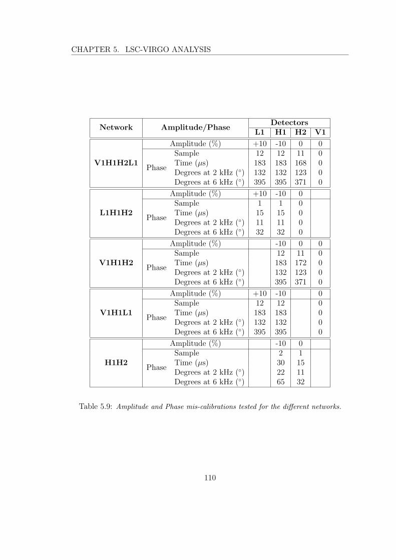
CHAPTER 5. LSC-VIRGO ANALYSIS
Network Amplitude/PhaseDetectors
L1 H1 H2 V1
V1H1H2L1
Amplitude (%) +10 -10 0 0
Phase
Sample 12 12 11 0Time (µs) 183 183 168 0Degrees at 2 kHz (◦) 132 132 123 0Degrees at 6 kHz (◦) 395 395 371 0
L1H1H2
Amplitude (%) +10 -10 0
Phase
Sample 1 1 0Time (µs) 15 15 0Degrees at 2 kHz (◦) 11 11 0Degrees at 6 kHz (◦) 32 32 0
V1H1H2
Amplitude (%) -10 0 0
Phase
Sample 12 11 0Time (µs) 183 172 0Degrees at 2 kHz (◦) 132 123 0Degrees at 6 kHz (◦) 395 371 0
V1H1L1
Amplitude (%) +10 -10 0
Phase
Sample 12 12 0Time (µs) 183 183 0Degrees at 2 kHz (◦) 132 132 0Degrees at 6 kHz (◦) 395 395 0
H1H2
Amplitude (%) -10 0
Phase
Sample 2 1Time (µs) 30 15Degrees at 2 kHz (◦) 22 11Degrees at 6 kHz (◦) 65 32
Table 5.9: Amplitude and Phase mis-calibrations tested for the different networks.
110

5.4. EFFECTS OF CALIBRATION SYSTEMATICS ON RESULTS
of systematic uncertainties. The rms fluctuations of these different detection ef-ficiency are then estimates of one sigma uncertainties on the detection efficiencydue to amplitude calibration uncertainties.
The assumption of Gaussian distribution is coarse and it is good only for 1σestimates. However, this procedure is particularly well suited to fold calibrationsystematics in the results of coherent searches. In fact, in coherent searches it isdifficult to select a priori which micalibration conditions may give worst results:in addition to the naive worsening due to a systematic underestimation of the h(t)data streams a coherent algorithm sensitive also to mis-balance in calibrationsamong detectors.
The actual MDC simulations have been performed on the JW1 data set to savecomputational time, since detection efficiency of JW1 data is representative of allthe S5Y2/VSR1 period.
Figure 5.16: Efficiency curves (top) and Hrss10-50-90% (bottom) resulting from Gaus-sian mis-calibrated tests. The error bars on efficiency are calculated from analyses madeselecting randomly 18 values of mis-calibrations sampled from the Gaussian distribution.V1H1H2L1 on the left and L1H1H2 on the right.
111

CHAPTER 5. LSC-VIRGO ANALYSIS
Figure 5.17: Hrss 10-50-90% for selected amplitude (left) and phase (right) mis-calibration effects. From top to bottom: V1H1H2L1, L1H1H2, V1H1H2, V1H1L1, H1H2.
5.5 Sanity and Consistency checks
Checks on results are useful to verify the correctness of work. A comparisonbetween odd and even lags, for instance, gives an idea on the quality to the
112

5.5. SANITY AND CONSISTENCY CHECKS
choice of post-production thresholds (consistency). Other checks (loud injec-tions, events reconstructed outside Category II segments) can test for bugs in thepipeline (sanity).
5.5.1 Events reconstructed outside Category II segments
Central time of reconstructed events should occur within the useful science data(Category II segments), otherwise this could be an alarm for bugs in the pipeline.This check has been performed both for background and SGQ9 simulations. Wefound a small fraction of events oustide the Category II segments (Tab. 5.10).Analysing the reconstructed times of these events, we found that their differencesbetween the start (or stop) of the nearest segment is less than 20 ms. This isconsistent with the cWB method to select time periods. The algoritm selectstime (and also frequency) making boundary cuts on time-frequency planes, afterthe application of the Wavelet Transform. This selection is not exactly appliedto the desired time, but it is approximated to the time resolution of the waveletdecomposition level at which we apply the boundary cuts. Starting from a samplerate of 12800 Hz and using from 4 to 9 decomposition levels, the maximum timeresolution is about 40 ms. So we can expect a small fraction of events with acentral time outside of the segments less than half this value. This because pixeltime is centered on the pixel.
NetworkBackground Simulations
Total Outside Total OutsideV1H1H2L1 5857829 218 803845 182L1H1H2 1134043 3 1223954 12V1H1H2 398698 4 165665 58V1H1L1 2201361 117 61358 25H1H2 504 0 288947 0
Table 5.10: Number of events with a central time outside Category II for Backgroundand SGQ9 simulations.
5.5.2 Consistency between odd and even lags
The tuning and estimation sets for each network should be two indipendent samplesof the accidental background distribution. We use the tuning set to choose post-production thresholds and the estimation set to calculate false alarms avoidingany possible statistical biases introduced by the tuning process. Before applying
113

CHAPTER 5. LSC-VIRGO ANALYSIS
post-production thresholds to the zero lag, we verify if the statistical properties ofthe two samples match for all the networks (excluding H1H2 network). Fig. 5.18shows the comparison between odd (black) and even (red) false alarm rate as afunction of ρth. Rate behaviour is compatible between odd and even lags for allnetworks except for the V1H1L1 one.
Figure 5.18: Consistency between odd (black) and even (red) lags background rate as afunction of ρth for different newtork. From left to right and tob to bottom: V1H1H2L1,L1H1H2, V1H1H2, V1H1L1.
We investigate the cause of this behaviour and we find a bump of noisy eventswith high ρ and cc (Fig. 5.19, left). These events are well localized in time (Fig.5.19, right), so we suspect a non standard behaviour of some instruments notspotted by the Data Quality cuts. This inconsistency between odd and even lagsfor this configuration is an evidence that the statistical uncertainties estimated forthe odd and even sets are underestimated. So we decided to set more restrictivethresholds using also the information from the even lag set, which dominates theempirical distribution of the loudest accidental events.
114

5.5. SANITY AND CONSISTENCY CHECKS
Figure 5.19: Scatter plot of ρ and cc (left) and ρ versus time (right) for the V1H1L1estimation set. The plot on the left reporst events with cc > 0.5.
5.5.3 Missing Loud Injections
We call “Loud Injections” the ones with the highest hrss amplitude at earth, cor-responding to the largest amplitude factor of the MDC injections. In fact, giventheir high hrss level, we espect that these loud injections should be correctly iden-tified by the analysis, with a few exceptions in case they occur from polarizationand sky locations which show a very unfavorable antenna pattern.
Simulation tests show a low number of missing lound injections. There aretwo ways which a Loud Injections can be missed: either the algorithm fails toreconstruct it, or it misses it because it not pass the post-production thresholds(Tab. 5.11).
Network Injected Found Not Pass Not RecV1H1H2L1 58613 58024 563 26
99% 0.96% 0.04%L1H1H2 104523 102356 1867 300
97.9% 1.8% 0.3%
Table 5.11: Loud Injections for V1H1H2L1 and L1H1H2: Injected, Found, Recon-structed but not passing Thresholds (Not Pass), Not Reconstructed (Not Rec).
We can verify that the events that are not reconstructed by the algorithmhave unfavourable antenna patterns. Whereas, events not passing post-productionthresholds shows a high disbalance among reconstructed signal energies in differentdetectors. Fig. 5.20 report on the left the value of |f×|/|f+| in the DominantPolarization Frame: events that are not reconstructed have source sky positions
115

CHAPTER 5. LSC-VIRGO ANALYSIS
where this value is almost null. On the right there is a scatter plot of V1 andH1 SNRs. Black points are reconstructed events passing threholds, instead redpoints are reconstructed events not passing thresholds. This last group shows ahigh disbalance on detectors SNR values.
Figure 5.20: Left: Fraction of plus and cross antenna pattern defined in the DPF. Blackdots are not reconstructed events. Right: V1 SNR versus H1 SNR for reconstructedevents passing (black) and not passing (red) thresholds.
5.5.4 Comparison with LF search
Low and High Frequency analyses have an overlapping frequency band between1280 and 2048 Hz. This overlapping band can be used to verify the consistencybetween the two analyses. We remind that post-production thresholds are notequal between LF and HF searches, because sensitivity curves and glitches dependon frequency (LF search has performed two separate tunings for frequency band[0Hz, 200Hz] and [200Hz, 2048Hz]). Discrepancies in the final detection efficienciesfor waveforms in the common bandwidth should be small, given the similar choiceof post production thresholds. For SGQ9 we have two common waveforms inthis frequency band: SG1615Q9 and SG2000Q9. We report in the Tab. 5.12the comparison of Hrss50% and Hrss90% for each network, values are compatible.However, we expect more discrepancies on the SG2000Q9 waveform, due to thefrequency band choice on the LF: [64, 2048] Hz. In fact, because of this frequencyband selection, about a 40% of the signal is lost (without taking into account thenoise). This could causes a loss on efficiency, especially for less energetic signals(lower values of injected hrss). So, we expect worse values of Hrss50% and Hrss90%for the LF results, as it is on Tab. 5.12.
116

5.6. RESULTS
Network WaveformLF (10−21 1/
√Hz) HF (10−21 1/
√Hz)
Hrss50% Hrss90% Hrss50% Hrsss90%
V1H1H2L1SG1615Q9 3.08 8.51 3.07 8.26SG2000Q9 4.43 12.4 3.94 10.4
L1H1H2SG1615Q9 3.32 14.9 3.88 16.8SG2000Q9 4.76 20.5 3.88 16.8
V1H1H2SG1615Q9 3.18 14.6 3.55 12.6SG2000Q9 5.40 22.5 4.42 17.5
V1H1L1SG1615Q9 4.62 1.47 4.76 1.74SG2000Q9 5.74 1.63 5.93 1.57
H1H2SG1615Q9 3.60 17.8 4.11 19.6SG2000Q9 5.02 23.7 5.08 23.7
Table 5.12: Comparison between Hrss50% and Hrss90% for LF and HF searches. TheSG2000Q9 shows in general larger differences, due to the fact the for the LF it is applieda frequency band selection on [64, 2048] which cuts about 40% of the signal.
5.6 Results
Once chosen the post-production thresholds for each network and performed theabove checks on the analysis, we are ready to analyze the on-source data. For eachnetwork we apply post-production thresholds to zero lag triggers and we verify itthere are candidate surviving the thresholds.
In case candidate events are found above the final thresholds, they would beconsidered for further investigations. In particular their false alarm rate wouldbe estimated against the empirical distribution of accidental events by ranking ac-cording to their ρ, and eventually excluding to a detection check list (DQ CategoryIII, see Sec. 5.1.1) whose aim is to perform deeper sanity checks and provide a pos-teriori information on the characteristics of the detectors and of the reconstructedsignal which could help in assessing an a posteriori confidence or plausibility for aGW or mondane nature of the candidate. In fact, the statistical study esplainedabove is not able to discriminate the nature of selected candidates, in particulara GW signal or a foreground event, the detection check list should help to shedlight on the physical source of the candidate signal.
Moreover, the candidate is checked with the “Blind Injection”, which is a list ofhardware injections not considered by DQ. These injections times are not unveileduntil the boxes are opened and they are used as a check on the algorithms perfor-mances. Blind injections have the same characteristics of an expected GW signal,so they should be detected and considered candidate events if strong enough, unlessthey occur at times later excluded by DQ vetoes. Unfortunately, when they are
117

CHAPTER 5. LSC-VIRGO ANALYSIS
injected, DQ segments are not ready, so it is possible that the blind injections areexcluded by the DQ vetos, and so they are not reconstructed by each algorithm.
If no events pass post-production thresholds, or if no candidates are acceptedas GW detection candidates, the results of the counting experiment will be used toset upper limits on the rate on GW events. This is accomplished by setting a upperlimit to the counting experiment according to the unified approach by Feldmanand Cousins [113]. Then this upper limit is interpreted in terms of rate versussignal strength at earth per each waveform by taking into account the measureddetection efficiency and the observation time. Here the rate of GWs is intendedas the random rate of a Poisson point process.
For the five networks analysed, we have null results on zero lag, i.e. nocandidate events. Fig. 5.21 shows the comparison between rate as a functionof ρth for background (black) and zero lag (red). The distributions of eventsrate versus rho at zero lag are in agreement with the measured distributions ofaccidental events within the expected statistical uncertainties. The events herehave been selected above the ccth and the comparison have been performed, usingall reconstructed triggers, below the ρth threshold. The zero lags appear thereforejust as samples of the expected accidental distributions. Moreover, a null resultsin all the trials is in agreement with the overall false alarm probability (FAP) ofthe search, which is about FAP ≈ 7.089 · 10−2.
In fig. 5.22 there are the efficiency curves for SGQ9 waveforms. These figuresare calculated at the final post-production thresholds.
From these results we can calculate upper limits for the injected waveforms.Upper limits is a confidence interval: in particular the upper limit will ensurea chosen conservative coverage, i.e. results would surpass by chance the upperlimit with probability less or equal to 1-coverage when only accidental events arepresent.
Upper limit can be easily calculated from a single pipeline considering therate of a Poisson-distributed process. We consider an experiment that measuresthe number of events of a specific random process that occurs in a time T. Weintroduce the following quantities: a mean rate µ of foreground events (that occurindependently from each others and is unknown); the efficiency ε of successfullydetecting any given event; a mean number b of background events in the time T.We assume that the total number of events (foreground plus background) countedin a given time is Poisson distributed. So, the probability of detecting N eventsover the full period T is given by:
P (N |ελ+ b) =
((ελ+ b)N
N !
)e−(ελ+b) (5.4)
where we have defined λ = µT as the expected mean number of foreground events.
118

5.6. RESULTS
Figure 5.21: Rate versus ρth at the final ccth for the network. From left to righ and topto bottom: V1H1H2L1, L1H1H2, V1H1H2, V1H1L1, H1H2.
The Feldman-Cousins approach [113] is to define a confidence interval [µ1, µ2]which is a member of a set, such that set has the property that:
P (µ) ∈ [µ1, µ2] = α (5.5)
Here, µ1 and µ2 are functions of the measured variable and the Eq. 5.5 refers tothe varying confidence intervals from an ensemble of experiments with fixed µ. Fora set of confidence intervals, Eq. 5.5 is true for every allowed µ. If the Eq. 5.5is satysfied, then we say that the intervals covers µ at the stated confidence, orequivalently, that the set of intervals has the correct coverage.
119

CHAPTER 5. LSC-VIRGO ANALYSIS
Figure 5.22: Efficiency curves at final ρth and cc for the network. From left to righ andtop to bottom: V1H1H2L1, L1H1H2, V1H1H2, V1H1L1, H1H2. In the table of eachfigure are reported the Hrss50% values for each waveforms.
So, selected a confidence level α and given n measured events, the frequentistupper limit λα at a confidence level α is the value at which there is a probability
120
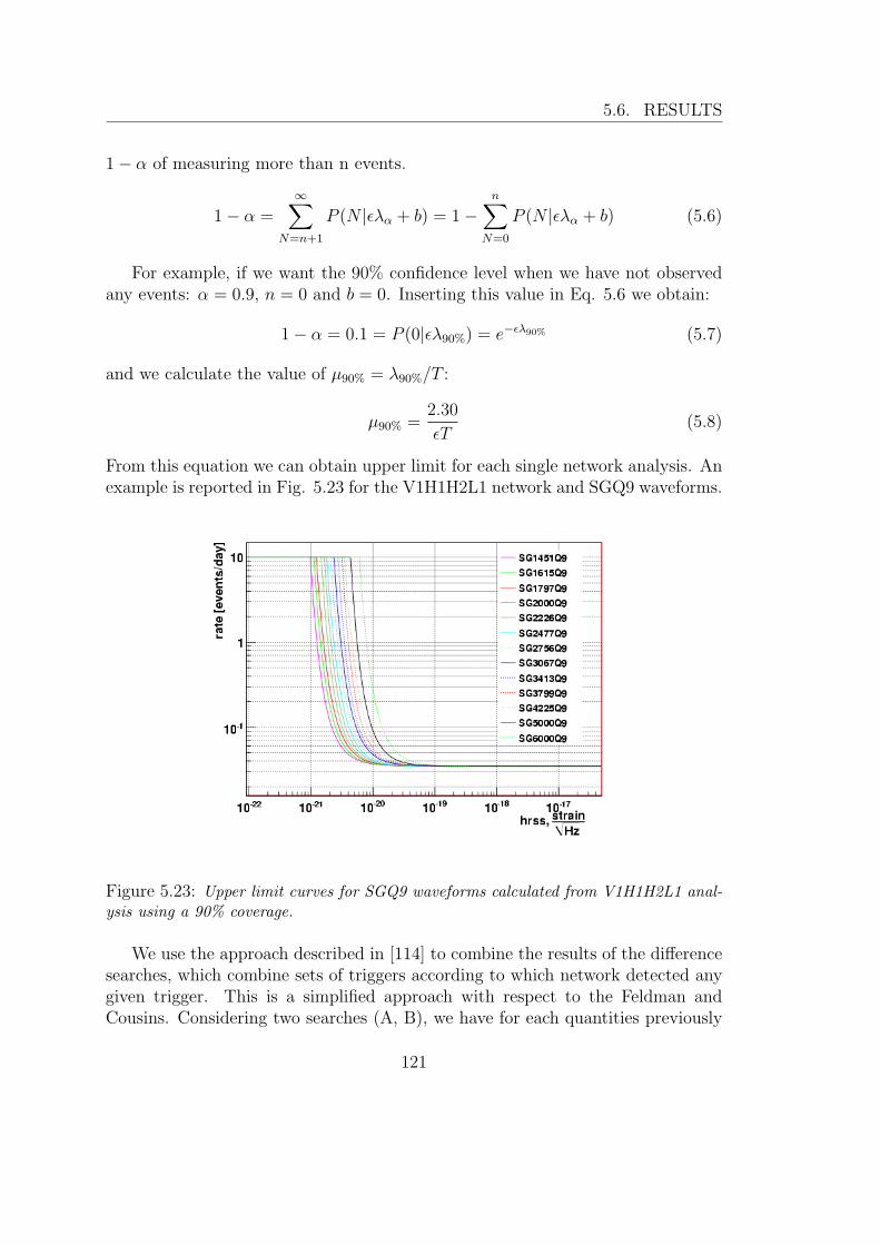
5.6. RESULTS
1− α of measuring more than n events.
1− α =∞∑
N=n+1
P (N |ελα + b) = 1−n∑
N=0
P (N |ελα + b) (5.6)
For example, if we want the 90% confidence level when we have not observedany events: α = 0.9, n = 0 and b = 0. Inserting this value in Eq. 5.6 we obtain:
1− α = 0.1 = P (0|ελ90%) = e−ελ90% (5.7)
and we calculate the value of µ90% = λ90%/T :
µ90% =2.30
εT(5.8)
From this equation we can obtain upper limit for each single network analysis. Anexample is reported in Fig. 5.23 for the V1H1H2L1 network and SGQ9 waveforms.
Figure 5.23: Upper limit curves for SGQ9 waveforms calculated from V1H1H2L1 anal-ysis using a 90% coverage.
We use the approach described in [114] to combine the results of the differencesearches, which combine sets of triggers according to which network detected anygiven trigger. This is a simplified approach with respect to the Feldman andCousins. Considering two searches (A, B), we have for each quantities previously
121

CHAPTER 5. LSC-VIRGO ANALYSIS
introduced three subsets: A, B, AB. For instance: nA is the number of eventsdetected by search A but not by B; nB is the number of events detected by searchB but not by A; and nAB is the number of events detected by both the searches.The same definitions are applied for the efficiencies (εA, εB, εAB). This can beeasily extendend to a general number p of searches, where we have 2p − 1 distintcombinations by which an event may be detected.
Introducing the vector notations ~N , ~ε and ~b whose components i = {1, ..., q}refer to different searches, we have:
P ( ~N |λ~ε+~b) =
p∏i=1
P (Ni|λεi + bi) (5.9)
To set a upper limit, one must decide a priori how to rank all possible obser-vations, so as to determine whether a given observation contains more or fewerevents than some other observations. Chosen the ranking function ζ(n), the rateupper limit Rα at confidence level α is given by:
1− α =∑
ζ( ~N)≤ζ(~n)
P ( ~N |~ε, Rα~T ) (5.10)
where P ( ~N |ε, Rα~T ) is the prior probability of observing ~N given the true GW rate
Rα, the livetimes of different data sets ~T and the detection efficiencies ε. The sumis taken over all N for which ζ( ~N) ≤ ζ(~n), i.e. over all possible outcomes ~N thatresults in fewer events than were actually observed.
For our case, we combine upper limits from the same pipelines applied todifferent networks which operates in disjoint time periods. So, the combinationis simplified, because it is not possible to detect the same event from differentnetworks (AB case mentioned above is not possible). So the formula assumes thesimple form:
µTOT90% =2.30∑i εiTi
(5.11)
where i refers to the networks.An example on the combinations of multiple pipelines for the SG3067Q9 is
provided in Fig. 5.24.The final upper limits for the SGQ9 MDC set calculated combining all the
networks involved are shown in Fig. 5.25
In this work we have summarized results of the all-sky search for gravitationalburst signal performed on the LIGO S5 second year and Virgo VSR1 data collectedin 2006-2007, on the frequency band [1280, 6000] Hz, applying the Waveburstalgorithm. The quality of the data and the sensitivity of the search algorithms have
122

5.6. RESULTS
Figure 5.24: Upper limit curves for SG3067Q9 combined from single networks using a90% coverage.
Figure 5.25: Upper limit curves for SGQ9 combined from single networks using a 90%coverage.
improved since similar searches of the previous LIGO S4 run [115] and even sincethe first year of S5 [116, 117]. This is reflected in an improved strain sensitivitywith Hrss50% as low as 5.6 · 10−22 1/
√Hz for certain LF waveforms, compared to
123

CHAPTER 5. LSC-VIRGO ANALYSIS
best values of 1.3·10−21 1/√Hz and 6.0·10−22 1/
√Hz for S4 and S5Y1 respectively.
Moreover, the S5Y2/VSR1 search also covers an extendend frequency band up to6 kHz, and the Hrss50% for S5Y2/VSR1 is improved of about 30% respect to S5Y1high frequency.
No plausible gravitational wave candidates have been identified in this search.Combined with the S5Y2 results, which had comparable observation time, thisyields an improved upper limit on the rate of bursts of 2.2 events per year at 90%confidence for the [2000, 6000] Hz band, which is about an half with respect to theS5Y1 upper limit of 5.4 per year for the frequency band [1000, 6000] Hz.
124

Conclusions and future prospectives
Gravitational Wave physics is a continuos improving science field that could givemany informations on the astrophysical objects and their caracteristichs that arenot available from electromagnetic radiation. However, the weak interaction of theGW with the matter is a huge obstacle on the GW detection.
This is the main reason which forces the scientific community to develop highsentivity intruments and search algorithms to allows the possibility to identify witha sure reliability a GW detection.
In spite of the great effort of scientists addressed to this goal, a GW detectionhas not yet declared. This creates also a lack of comparison term, which makesmore difficult to establish a sure method to declare a detection of a GW. More-over, the complicated resolution of Einstein’s equation applied to astrophysicalprocesses, often requires the use of approximated numerical simulations, whichcannot describe all the possible scenarios of GW generating processes. This ex-plains the importance of introducing an algorithm which does not require particularassumptions on the expected signal we want to detect, i.e. what we have called inthis thesis un-modelled search.
Moreover, these issues are strictly related to the importance of improving de-tector perfomances. In particular, the GW community planned to improve by anorder of magnitude the sensitivity of LIGO and Virgo detectors with respect to thepresent ones (Advanced LIGO [19] and Advanced Virgo [118]). This would allowto increase by the same order the observable horizon and by three orders of magni-tude the observable sky volume, with an expected rate of 10s/100s events per year.
In this work we have presented the Waveburst algorithm, focusing on theCoherent version, we have realised, in fact, that coherent pipelines are by far moreefficient on discarding false alarms respect to the incoherent ones. Waveburst usesthe wavelet properties and the likelihood ratio approach to identify significanttriggers in the data stream, and it is able to adapt the search to the spectraland directional sensitivity of the network (use of regulator) or make particularassumptions on the waveform characteristics (use of constrains).
We have applied the Coherent Waveburst algorithm to the LIGO-Virgo collab-
125
CHAPTER 5. LSC-VIRGO ANALYSIS
oration detector on the first long term observation of LSC and Virgo detectors,S5Y2/VSR1, to search for GW transient signals in the High Frequency band-width (2 ÷ 6 kHz). With respect to previous analysis in the same bandwidth,this is the first coherent analysis, which is an important feature when detectorswith so different directional sensitivities are in joint observation. The analysis hasbeen performed on data from different network configurations, i.e. combinationsof the four involved detectors (L1, H1, H2, V1). Each configuration is analysedin its exclusive livetime, i.e. the observation time covered by only that specificconfiguration of detectors in science mode. Only networks with enough live timehas been analysed (L1H1H2V1, L1H1H2, V1H1H2, L1H1V1, H1H2). For eachnetwork, background and simulations tests have been performed, in such a wayto give a reliable confidence of a possible detection and to give an interpretationof the results in terms of some classes of signal models. Sine Gaussian waveformshave been used as reference efficiency waveforms for the tuning of the post pro-duction parameters, whereas we have tested also the efficiency detection for moreinteresting astrophysical signals (such as Ring Down waveforms or Supernova Col-lapse). No events candidate have been found. The direct scientific output is thebest upper limit for this bandwidth.
The pipeline version used for the S5/VSR1 analysis had the most advancedperformances available for what concerns the capability of discriminating signalsfrom accidental triggers. However, its performances for what concerns the recon-struction of the characteristics of an identified GW candidate were still far fromoptimal. We then started a research and development study to improve the ca-pabilities of the algorithm to estimate the GW direction and we took part tothe project Position Reconstruction Challenge, whose goals was to stimulate pro-gresses on position reconstruction with LSC and Virgo detectors and compare theresults from different algorithms. We achieved progresses of one order of magni-tude better with respect to previous angular reconstruction. Today, error anglesfor a wide class of signal waveforms are typically of the order of one degree at highsignal to noise ratio. However, further progresses are needed to easy the start ofa multimessenger astronomy, in particular to allow a follow up of GW candidatesby other astronomical instruments from X and gamma-ray satellites to wide fieldsoptical based instruments.
The current work on reconstruction capabilities is also targeting procedures toset sky Error Region on source position coverage (probability of detecting signal).In addition, to the position reconstruction problem, we recently started to addressthe issue of reconstructing the waveform information from detected signals, whichwill be as important as source location for the GW astronomy.
126

5.6. RESULTS
We are currently analyzing the second long term observation of the LSC-Virgodetectors (started on July 2009, planned to the end of 2010). The first results arebeing internally reviewed by the collaboration. For this transient signal search, themain structure of the algorithm has been improved in other two aspects which arerelevant for the identification of signal candidates. Any position in the earth framecan now be used as reference for the delays in arrival time of the GW wavefront,so that the Likelihood Sky Map can be computed from any such reference, e.g.any detector. The time slide procedure to sample the background has been gener-alized so that any detector can be time shifted with respect to the others. Thesesymmetrizations of the scheme of the pipeline allow a much better estimation ofthe accidental background of the searches both from what concerns statistical andsystematic errors.
127


Appendix A
Pipeline line by line
This is a summary of the principal actions of the pipeline, following line by linethe C++ macro. Some commands are applied only for simulation tests injectingMDC. In this case we use the label “(SIM)”.
InizializationInitialization of the useful elements: mother wavelet, arrays (time, MDC, noise,detectors).Inizialization of the network and all the elements connected to it.Inizialization of trees1: mdc, livetime, bursts, variability, noise.Reading of the file containing information about time and data for the selectedjob. The pipeline calculated the start and stop of the segment.Correction of lags number to avoid time shifts greater than length segment.NET.setTimeShifts: set parameters for time shift analysis.(SIM) MDC log file is read.Data frames are uploaded, the interesting bandwidth is selected using waveletdown conversion and then data are saved at a chosen wavelet decomposition level.6 kHz Down conversion is applied at this step.(SIM) Same procedure as the previous line for MDC data frames.Assignations output and temporary ROOT file names.Starting of loop for amplitude injection factors. The following commands arerelated to a single amplitude factor.
Data ConditioningUploading of Down Converted data saved previously.(SIM) Uploading of MDC Down Converted data saved previously. Data amplitudesare multiplied for the amplitude factor. MDC is injected in the noise data stream.
1A tree is a ROOT object which records for each event all its characteristics (called leaves)for a simple visualization.
129

APPENDIX A. PIPELINE LINE BY LINE
Line Predictor Filter and Whitening of the data stream.A band pass filter is applied, to select the frequency band of interest previouslydeclared (parameter file).NET.SetVeto: set time periods which are not processed because excluded by vetofile.
Inizialization of the output filesFinal ROOT files are created, and finals trees are associated to them.
Start of the coeherent searchStarting of loop for TF levels. The follosing commands are related to a singledecomposition level.Uploading of time delay filters.NET.threshold: calculates Waveburst threshold as a function of resolution andmaximum delay.NET.coherence: selects time-frequency samples.NET.cluster: produces time-frequency cluster as a swingle time-frequency resolu-tion.NET.likelihood(E)Ending of loop for TF levels.
Supercluster analysispwc=NET.getwc, pwc->supercluster: constructs the superclusters.NET.events: returns number of events.
LikelihoodNET.likelihood()NET.netcut(netRHO,r,0,1): selection of clusters based on threshold on rho.NET.netcut(netCC,c,0,1): selection of clusters based on threshold on network cor-relation coefficient.NET.events: return number of events.(SIM) NET.printwc: save the properties of the events.
Save data in root fileEvents are saved in output files.Temporary files used for the analysis are deleted.
A.1 NET.Coherence
This functions selects the pixels with compose the clusters, tagging them with aboolean array of values. Only the selected pixels are used to compute likelihood(NET.likelihood function).
Without considering line by line this function, the procedure of selecting pixelis based on the coherence between corresponding pixels belonging to different de-
130

A.2. NET.LIKELIHOOD
tectors. The first detector is used as reference one, and its pixels are tagged by theboolean array. The function takes one pixel of the first detector and it calculatesthe corresponding pixels of the other detectors associated to a certain position inthe sky, using the delay time filters (Cap. 3.2.5). For a pixel of the first detectorlocated at the time t0, the corresponding pixels of another one refer to a timeperiod [t0 − δt10, t0 + δt10], where δt10 is the maximum delay time between thetwo detectors. This means that the generic pixel t0 of the reference detector iscombined with:* N1 pixels inside [t0 − δt10, t0 + δt10] of detector 1,* N2 pixels inside [t0 − δt20, t0 + δt20] of detector 2,and so on for all the detectors involved.
Each set of the type: {t0, t1k, t2k, ...} indicates a position (k) in the sky.Varying each tik, i > 0 inside the periods [t0 − δt1i, t0 + δt1i] we can select all thesky positions. The pixel t0 is selected if there is at least position in the sky wherethe sum of square amplitude of the pixels t0, t1, t2, ... is greater than a definitethreshold.
This procedure is repeated for all the pixels of all the decomposition levels.
This function is computationally heavy, so the pipeline uses some tricks todecrease the computational loading. Consider the pixel t0, we have to calculateall the quantities Sk =
∑Ni=0A(tik), where N is the number of detectors and A(p)
is the amplitude of the pixel p. If the maxk Sk > threshold the pixel is selected.We can write Sk = A(t0) +
∑Ni=1A(tik) so the previous condition can be written
maxk S′k > threshold −A(t0) where S ′k =
∑Ni=1A(tik). This allows us to reduce
computational load when applying time shift. In fact, if we have M lags of ∆ timeshift, the maxk S
′k has the same value for the different t0 +m∆ (0 ≤ m ≤M) and
we can calculate one time for all the shifts applied.Computational time is reduced also considering that maxk S
′k <
∑Ni=1 maxk A(tik),
so we can make a pre-selection of pixels considering the disequality∑N
i=1 maxk A(tik) >threshold. Pixels that do not survive to this disequality cannot surely be tagged asusable. This pre-selection reduces significantly the number of pixels to be selected(a factor of the order of 103).
A.2 NET.likelihood
This function calculates the likelihood ratio on the cluster composed by the se-lected pixels. The NET.likelihood function is applied twice in the pipeline, thefirst time (when it accepts the parameter ’E’) it operates a selection on the clustereliminating the ones which have a large discrepancy between the detector con-tributes.
131

APPENDIX A. PIPELINE LINE BY LINE
The second times the function is applied the algorithm calculates the likelihoodratio for each event (an event is represented by the correspondind super cluster)over all the sky locations. The maximum value of the likelihood location overthe sky is considered as the starting point to calculate all the parameters that weassociate to the reconstruct events. The likelihood ratio is calculated according tothe chosen regulator and constrain (See Chapter 3.1.4 and Appendix B).
132

Appendix B
Relation between a general frameand the DPF
We have introduced the DPF in the section 3.1.2, demonstrating that in thiscoordinate the Likelihood functional assumes a simple form. However, it is notnecessary to transpose all the vectors in this frame, but it is possible to calculatethe Likelihood functional and all the interesting quantities also in the generalframe. We remember now useful consideration.
� In the general frame, the vectors f+ and f× are not orthogonal.
� The transformation between the general frame and DPF are given by:
f ′k+ = fk+Cos(γ) + fk×Sin(γ)f ′k× = −fk+Sin(γ) + fk×Cos(γ)
(B.1)
whereCos(2γ)|Aσ|2 = (f 2
+ − f 2×)
Sin(2γ)|Aσ|2 = 2(f+ · f×)(B.2)
� We are more interested in direction of vectors than in module, because wecan always normalize them. This means that sometimes we will calculatethe quantity αv instead of v if it is easier computable.
� The Maximum Likelihood is given by:
L =(X · u)2
|u|2(B.3)
where u is defined in the (f ′+, f ′×) plane by regulators.
� (f ′+, f ′×) and (f+, f×) are the same plane, because the f ′+ and f ′× vectors arelinear combinations of f+ and f×.
133

APPENDIX B. RELATION BETWEEN A GENERAL FRAME AND THEDPF
From these considerations we can obtain the formula of the Likelihood functionalin the general frame, calculating the expression of vector u in the general framefor the different regulators considered.
The vector u can be expressed as a linear combination of the two vectors f+
and f×:
u = ucf+ + usf× (B.4)
so in the following considerations we will find the expression of uc and us for thedifferent regulators definitions.
Figure B.1: Dominant Polarization Frame, v is a vector perpendicolar to u in the plane(f ′+, f ′×)
B.1 Weak regulator
The weak regulator consider u as the projection of X in the (f+, f×) plane.Because f+ and f× are not orthogonal, we cannot write u = u·f+
|f+| e+ + u·f×|f×| e×
1
as we can do in the DPF. We can avoid this problem using the vector product.
1e+ and e× are versor with the same direction as f+ and f×.
134

B.1. WEAK REGULATOR
Referring to Fig. B.1, we consider the vector f+×f×, which describe the sub-spaceorthogonal to the plane (f+, f×). Then we define the vector v
v = X × (f+ × f×) (B.5)
This vector is on the plane (f+, f×) and it is orthogonal to X. So, if we define thevector
u = −v × (f+ × f×) (B.6)
u is on the plane (f+, f×) (because it is orthogonal to f+×f×) and (apart from themodule) it is the projection of X (because it is othogonal to v, which is orthogonalto X). This is the vector we are interested in, except for the module, but we candisregard about it.
Mathematically, we use the property of triple vector product:
a× (b× c) = b(a · c)− c(a · b) (B.7)
we have:
u = −v × (f+ × f×) = −f+(v · f×) + f×(v · f+) (B.8)
Comparing this equality with u = f+uc+f×us we have: uc = −v·f× and us = v·f+.Remebering the definition of v:
v = X × (f+ × f×) = f+(X · f×)− f×(X · f+) = f+X× − f×X+ (B.9)
where we have defined the quantities: X+ = X · f+ and X× = X · f×. Then:
−v · f× = −(f+X× − f×X+) · f× = X+(f× · f×)−X×(f+ · f×)v · f+ = (f+X× − f×X+) · f+ = X×(f+ · f+)−X+(f× · f+)
(B.10)
Finally:
uc(weak) = X+(f× · f×)−X×(f+ · f×)us(weak) = X×(f+ · f+)−X+(f× · f+)
(B.11)
135
APPENDIX B. RELATION BETWEEN A GENERAL FRAME AND THEDPF
B.2 Soft regulator
The soft regulator defines u = (X · f ′+)f ′+ + (X · f ′×)f ′×. So we can write:
u = [X · (f+Cos(ψ) + f×Sin(ψ))](f+Cos(ψ) + f×Sin(ψ))+
+ [X · (−f+Sin(ψ) + f×Cos(ψ))](−f+Sin(ψ) + f×Cos(ψ)) =
= [X+Cos(ψ) +X×Sin(ψ)](f+Cos(ψ) + f×Sin(ψ))+
+ [−X+Sin(ψ) +X×Cos(ψ)](−f+Sin(ψ) + f×Cos(ψ)) =
= [X+Cos2(ψ) +X×Cos(ψ)Sin(ψ) +X+Sin
2(ψ)−X×Cos(ψ)Sin(ψ)]f++
+ [X+Cos(ψ)Sin(ψ) +X×Sin2(ψ)−X+Cos(ψ)Sin(ψ) +X×Cos
2(ψ)]f× =
= X+f+ +X×f×(B.12)
So, the definition of u for the soft regulator is:
uc(soft) = X+
us(soft) = X×(B.13)
B.3 Hard regulator
The hard regulator assumes that u has the same direction as f ′+ in the DPF. So,u = f ′+, and from Eq. 3.17 we have that f ′+ = f+Cos(γ) + f×Sin(γ). Because weare interested only in direction, we calculate the quantity Cos(γ)u instead of u:
Cos(γ)u = f+Cos2(γ) + f×Sin(γ)Cos(γ) = f+
1
2[1 + Cos(2γ)] + f×
1
2Sin(2γ)
(B.14)and from Eq. 3.21 we have:
Cos(γ)u = f+1
2
[1 +
f 2+ − f 2
×
|A2σ|
]+ f×
f+ · f×|A2
σ|(B.15)
So, multipling by |A2σ| and discarding the factors on the left part we have the
expression for uc and us:
uc(hard) = 12|A2
σ|+ 12(f2
+ − f 2×)
us(hard) = f+ · f×(B.16)
136

B.4. MILD REGULATOR
B.4 Mild regulator
Finally the mild regulator defines u = f ′+±f ′×. We can repeat the same procedurefor the hard regulator.
Cos(γ)u = Cos(γ)(f ′+ ± f ′×) =
= (f+Cos2(γ) + f×Cos(γ)Sin(γ))± (−f+Cos(γ)Sin(γ) + f×Cos
2(γ)) =
= f+(Cos2(γ)∓ Cos(γ)Sin(γ)) + f×(Sin(γ)Cos(γ)± Cos2(γ)) =
= f+
[1
2
(1 +
f 2+ − f 2
×
|A2σ|
)∓ f+ · f×
|A2σ|
]+ f×
[f+ · f×|A2
σ|± 1
2
(1 +
f 2+ − f 2
×
|Aσ|2
)](B.17)
Multipling for |A2σ| and discarding the common factor, we obtain the final form:
uc(mild) = 12(|A2
σ|+ (f2+ − f 2
×))∓ (f+ · f×)us(mild) = (f+ · f×)± 1
2(|A2
σ| − (f 2+ − f 2
×))(B.18)
The ± sign depends on what quadrants of the f+,f× plane the X vector is pro-jected. So, if the projection of X is on the first or third quadrant the sign is +,otherwise this sign is −. This conditions can be expressed using the inequalitieson the Tab. B.1:
Condition Sign(X · f ′+)(X · f ′×) > 0 +(X · f ′+)(X · f ′×) < 0 -
Table B.1: Conditions for the choice of ± sign of the mild regulator
B.5 Intermediate regulators
It is possible to choose intermediate situations between regulators using variableparameters. For instance in the definition of mild regulators: uc(mild) = 1/2|A2
σ|+1/2(f 2
+ − f 2×) ∓ (f+ · f×) we can define a parameter called mild in the following
way: uc(mild) = 1/2|A2σ| + 1/2(f 2
+ − f 2×) ∓ mild(f+ · f×). Changing the value of
the parameter mild from 0 to 1 we can use an intermediate regulator from mild(mild=1) to hard (mild=0) definitions. Generally we can define an single definition
137

APPENDIX B. RELATION BETWEEN A GENERAL FRAME AND THEDPF
of uc and us including all the regulators:
uc(all) = softX++
+ mild(f+ · f×)gg+
+hard
(f 2+ + f 2
×)/2 + |A2σ|
[X+
(|A2
σ|+f 2
+ − f 2×
2
)+X×(f+ · f×)
]us(all) = softX×+
+ mild
(|A2
σ|+f 2
+ − f 2×
2
)gg+
+hard
(f 2+ + f 2
×)/2 + |A2σ|
[X×
(|A2
σ| −f 2
+ − f 2×
2
)+X+(f+ · f×)
](B.19)
where gg is defined as:
gg =1(
|Aσ|2 +f2+−f2
×2
)2
+ (f+ · f×)2
·
{[X×
(|A2
σ|+f 2
+ − f 2×
2
)−X+(f+ · f×)
]±
[X+
(|A2
σ|+f 2
+ − f 2×
2
)+X×(f+ · f×)
]}(B.20)
Using intermediate values of the parameters we can use superimposition ofregulators, in particular we can define a new parameter (δ) and varying this wecan choose a regulator o a superimposition between regulators (Tab B.2).
δ range Regulator soft mild hardδ = -1 soft 1 0 -1-δ=0
-1 < δ < 0 soft-weak 1 0 -1-δδ = 0 weak 1 δ=0 δ-1=-1
0 < δ < 1 weak-mild 1 δ δ-1δ = 1 mild 1-hard=1 1-hard=1 δ-1=0
1 < δ < 2 mild-hard 1-hard 1-hard δ-1δ ≥ 2 hard 0 0 1
Table B.2: Relationship between δ and parameter values to obtain regulators from Eq.B.19. Red cases refer to pure regulator definition, blue cases refer to superimpositionsbetween regulators.
138

Appendix C
Energy disbalance approximations
Equation 3.49 is an approximation of 3.47 for ψ ≈ 0. Reminding the quantitiesinvolved:
uk = uk0Cos(ψ) + vk0Sin(ψ)vk = ∂u
∂ψ= −uk0Sin(ψ) + vk0Cos(ψ)
qk = Xkuk − u2kh
pk = −∂qk∂ψ
= (2ukh−Xk)vk + u2k(X · v)/|u|2
(C.1)
where the index k refers to a certain detector, and the scalar product ( · ) substi-tutes the sum between indexes k, as we have previously introduced.
Now we approximate the definitions of pk and qk for small angles ψ. We remindthat in the limit ψ → 0, then Sinn(ψ) ∼ 0 for n ≥ 2:
Sin2(ψ) ∼ 0Cos2(ψ) = 1− Sin2(ψ) ∼ 1
(C.2)
The module of u remains constant changing the value of ψ angle, in fact this isonly a rotation on the plane. Matemathically:
∂|u|2
∂ψ=∂(u · u)∂ψ
= 2(u · v) = 0 (C.3)
139

APPENDIX C. ENERGY DISBALANCE APPROXIMATIONS
Considering the definition of qk and using the previous approximations:
qk = Xkuk − u2kh =
= Xk(uk0Cos(ψ) + vk0Sin(ψ))+
− (uk0Cos(ψ) + vk0Sin(ψ))2X · (u0Cos(ψ) + v0Sin(ψ))
|u|2≈
= Xkuk0Cos(ψ) +Xkvk0Sin(ψ)+
− (u2k0Cos
2(ψ) + 2uk0vk0Cos(ψ)Sin(ψ))(X · u0)Cos(ψ) + (X · v0)Sin(ψ)
|u0|2=
= Cos(ψ)
[Xkuk0 − u2
k0
X · u0
|u0|2
]+
+ Sin(ψ)
[Xkvk0 − u2
k0
X · v0
|u0|2− 2uk0vk0
X · u0
|u0|2
]=
= qk0Cos(ψ)− pk0Sin(ψ)
(C.4)
The approssimation for pk is calculated from its definition:
pk = −∂qk∂ψ
∼ − ∂
∂ψ(qk0Cos(ψ)− pk0Sin(ψ))
= q0Sin(ψ) + p0Cos(ψ)
(C.5)
140

Bibliography
[1] F. Acernese et al., The Virgo status, Class. Quantum Grav. 23 (2006) S635
[2] B.P. Abbott et al., LIGO, the Laser Interfometry Gravitational-Wave Obser-vatory, Rep. Prog. Phys.72 (2009) 076901
[3] H. Luck et al., Status of the GEO600 detector, Class. Quant. Grav. 23 S71
[4] R. Takahashi, Status of TAMA 300, Class. Quant. Grav 21 (2004) S403
[5] K. S. Thorne, Gravitational waves from compact bodies, in Proc. of IAU Sym-posiusm 165, Compact Star in Binaries, (1995)
[6] K. S. Thorne, in 300 Years of Gravitations, Hawking and W. Israel eds, Cam-bridge Univ. Press (1987)
[7] J. Hartle, Gravity, an introduction to Einstein’s general relativity, AddisonWesley, 2003.
[8] C. D. Ott, The gravitational-wave signature of core-collapse supernovae, ClassQuantum Grav. 26, 063001 (2009)
[9] E. Baron and J. Copperstein, Astrophys. J. 353, 597 (1990)
[10] H. A. Bethe, Supernova mechanism, Rev. Mod. Phys. 62, 801 (1990)
[11] H-T Janka et al., Theory of core-collapse supernovae, Phys Rep 442, 38 (2007)
[12] J.M LeBlanc and J.R. Wilson, Astrophys J. 161, 541 (1970)
[13] H Swai et al., Astrophys J 672, 465 (2008)
[14] A. Burrows et al., Multi-dimensional explorations in supernova theory, Phys.Rep. 442, 23 (2007)
[15] S. van den Bergh and G.A. Tammanm, Galactic and Extragalactic SupernovaRates, Ann. Rev. Astron. Astroph. 29, 363 (1991)
141

BIBLIOGRAPHY
[16] S. Andoet al, Astron. Astroph. 246, 47 (1991)
[17] L. Baiotti and L. Rezzolla, Challenging the Paradigm of Singularity Excisionin Gravitational Collapse, Phys. Rev. Lett. 97, 141101 (2006)
[18] L. Baiotti et al., On the gravitational radiation from the collapse of a neutronstars to rotating black holes, Class. Quantum Grav. 24, S187 (2007)
[19] P. Fritschel, Second generation instruments for the Laser Interferometer Grav-itational Wave Observatory (LIGO), Proceedings of SPIE, Vol. 4856, p. 282(2003)
[20] C. D. Ott, Stellar iron core collapse in 3+1 general relativity and the grav-itational wave signature of core-collapse supernovae, PhD Thesis UniversitatPotsdam, Germany
[21] R. Oechslin and H-J Janka, Gravitational Waves from Relativistic Neutron-Star Mergers with Microphysical Equations of State, Phys. Rev. Lett. 99,121102 (2007)
[22] K. Kiuchi et al., Longterm general relativistic simulation of binary neutronstars collapsing to a black hole, submitted to Phys. Rev. D, arXiv:0904.4551
[23] A. Buonanno et al., Detection template families for gravitational waves fromthe final stages of binary-black-hole inspirals: Nonspinning case, arXiv:gr-gc/0205122v3 (2006)
[24] N. Andersson e K.D. Kokkotas, Gravitational-wave astronomy: the high-frequency window, General Relativity and Quantum Cosmology, 2004.
[25] V. Ferrari, G. Minuitti and J.A. Pons, Gravitational waves from newly born,hot neutron stars, Mon. Not. R. Astron. Soc. 2006.
[26] V. Kalogera et al. Astrophys J. 601, L179 (2004)
[27] C. Kim et al., The Probability Distribution of Binary Pulsar CoalescenceRates., Astrophys J. 584, 985 (2003)
[28] K. T. Inoue and T. Tanaka, Gravitational Waves from Sub-Lunar-Mass Pri-mordial Black-Hole Binaries: A New Probe of Extradimensions, Phys. Rev.Lett. 91, 021101 (2003)
[29] S. E. Woosley, Astrophys. J. 405, 273 (1993)
[30] B. Paczynski, Astrophys. J. 494, L45 (1998)
142

BIBLIOGRAPHY
[31] A. I. MacFadyen and A. I. Woosley, Collapsars: Gamma-Ray Bursts andExplosion in “Failed Supernovae”, Astrophys. J. 524, 262 (1999)
[32] S. I. Blinnikov et alt., Sov. Astron. Lett. 10, 177 (1984)
[33] J. Goodman, Astrophys. J. 308, L47 (1986)
[34] J. Goodman et al., Astrophys. J. 314, L7 (1987)
[35] D. Eichler, Mon. Not. Roy. Astron. Soc. 335, 883 (2002)
[36] R. F. Stark and T. Piran, Gravitational-Wave Emission from Rotating Grav-itational Collapse, Phys. Rev. Lett. 55, 891 (1985)
[37] B. F. Schultz, Class. Quantum Grav. 16, A131 (1999)
[38] J. G. Jernigan, KiloHerts QPO and Gravitational Wave Emission as the Sig-nature of the Rotation and Precession of a LMXB Neutron Star Near Breakup,AIP Conf. Proc. 586, 805 (2001)
[39] H. J. Mosquera Cuesta and D. M. Gonzales, Bursts of Gravitational Radiationfrom Superconducting Cosmic Strings and the Nuetrino Mass Spectrum, Phys.Lett. B 500, 215-221 (2001)
[40] www.auriga.lnl.infn.it
[41] Ott C, Burrows A, Dessart L and Livne E, Physical Review Letters, 96 201102,2006.
[42] www.virgo.infn.it
[43] www.ligo.caltech.edu
[44] www.geo600.uni-hannover.de
[45] http://tamago.mtk.nao.ac.jp
[46] http://www.gravity.uwa.edu.au
[47] http:///www.lisa.jpl.nasa.gov
[48] R. V. Pound, Electronic frequency stabilization of microwave oscillators, Rev.Sci. Instrum. 17, 490-505 (1946)
[49] R. W. P. Drever et al., Laser phase and frequency stabilization using an opticalresonator, Appl. Phys. B 31, 97-105 (1983)
143

BIBLIOGRAPHY
[50] Virgo Collaboration, Extending the virgo gravitational wave detection banddown to a few Hz: metal blade springs and magnetic antisprings, Nucl. Instrum.and Meth. in Phys. Red. A, 394:397-408 (1997)
[51] J. N. Brune and J. Oliver, The seismic noise of the earth’s surface, Bull.Seism. Soc. Am. 49 (1959)
[52] Virgo collaboration, The virgo interferometer, Class. Quantum Grav. 14, 1461(1997)
[53] H. B. Callen and T. A. Welton, Phys. Rev. 83 (1951)
[54] C. Cagnoli, L. Gammaiotni, J. Kovalik, F. Marchesoni and M. Punturo, TheVirgo sensitivity curve, virgo note, Perugia March 1997
[55] M. Maggiore, Gravitational Wave Experiments and Early Universe Cosmol-ogy, arXiv:gr-qc9909001 (2000)
[56] S.Klimenko e G. Mitselmakher, A Wavelet method for detection of gravita-tional wave bursts, Class. Quantum Grav. 21 (2004) S1819-S1930.
[57] S. Klimenko et al., A coherent method for detection of gravitational wavebursts, Class. Quantum Grav. 25:S114029 (2008)
[58] S.Chatterji Multiresolution techniques for the detection of gravitational-wavebursts, Class. Quantum Grav. 21, (2004) S1809
[59] A. Clapson et al., EGC: a time-frequency augmented template-based methodfor gravitational wave burst search in ground based interferometers, Class.Quant. Grav 25:S035002 (2008)
[60] M.Bignotto et al., A cross-correlation method to search for gravitational waveburts with AURIGA-Virgo, Class Quantum Grav. 25, 114046 (2008)
[61] J. Markowitz et al., Gravitational wave burst source direction estimation usingtime and amplitude information, Phys. Rev. D 78 122003 (2008)
[62] F. Cavalier et al., Reconstruction of source location in a network of gravita-tional wave interferometric detectors, Phys. Rev. D. 78:082004 (2006)
[63] S. Klimenko et al., Waveburst, version 5, Technical Note LIGO-T050222-00-Z,Sept 25, 2005.
[64] S. Klimenko et al., Constraint likelihood analysis for a network of gravitationalwave detectors, Phys. Rev. D 72, 122002 (2005)
144

BIBLIOGRAPHY
[65] http://root.cern.ch
[66] S. Klimenko, I. Yakusin and G. Mitselmakher, Waveburst, LIGO noteT040040-00-Z
[67] S. Klimenko, I. Yakusin and G. Mitselmakher, Waveburst, S5 version, LIGOnote T060112-00-Z
[68] S. Klimenko, I. Yakusin and G. Mitselmakher, Waveburst, version 5, LIGOnote T050222-00-Z
[69] S. Mallat, A wavelet tour of signal processing, Academic Press, 1998.
[70] R. A. Mercer and S. Klimenko Visualising gravitational-wave event candidatesusing the Coherent Event Display, Class. Quantum Grav. 25, (2008) 184025
[71] R. A. Mercer and S. Klimenko, The Coherent Event Display, LIGO noteT080077-00-Z, 2008
[72] J. Sylvestre, Prospects for the detection of electromagenic counterparts to grav-itational wave events, Astrophys. J. 591, 1152-6 (2003)
[73] L. Li and B. Pacyznski, Astrophys. J. 507, L59-62 (1998)
[74] H. T. Janka and M. Ruffert, Detectable Signals from Mergers of CompactStars, ASP Conf. Ser. 263, 333 (2002)
[75] S. Rosswog, Mergers of Neutron Star-Black Hole Binaries with small MassRatios: Nucleosynthesis, Gamma-Ray Bursts, and Electromagnetic Transients,Astrophys. J. 634, 1202-13 (2005)
[76] J. Kanner et al., LOOC UP: locating and observing optical counterparts togravitational wave bursts, Class. Quantum. Grav. 25, 184034 (2008)
[77] N. Gehrels et al., Gamma-ray bursts in the Swift era, New Journal of Physics9, 37 (2007)
[78] E. Nakar, Short Hard gamma-ray Bursts, Physics Reports 442, 166-236 (2007)
[79] http://www.ligo.caltech.edu/docs/ScienceDocs/G/G080465-02/G080465-02.pdf
[80] A. Sadowsky et al., Simulations of Dynamo Action in Fully Convective Stars,Astrophys. J. 676, 1162-69 (2008)
145

BIBLIOGRAPHY
[81] J. s. Blooms et al, Astro2010 Decadal Survey Whitepaper, Coordinated Sciencein the Gravitational and Electromagnetic Skies, arXiv:0902.1527 (2009)
[82] http://gwdaw12.mit.edu
[83] http://cgwa.phys.utb.edu/gwdaw13/
[84] B. Abbott et al., Implications for the Origin of GRB 070201 from LIGOObservations, Astrophys. J. 681, 1419 (2008)
[85] B. Abbott et al., Search for gravitational waves associated with 39 gamma-raybursts using data from the second, third, and fourth LIGO runs, Phys. Rev. D77, 062004 (2008)
[86] B. Abbott et al., Search for Gravitational-Wave Bursts from Soft GammaRepeaters, Phys. Rev. Lett. 101, 211102 (2008)
[87] https://www.lsc-group.phys.uwm.edu/twiki/bin/view/Bursts/Online
[88] https://www.lsc-group.phys.uwm.edu/twiki/bin/view/Bursts/PosRec
[89] http://www.rotse.net
[90] http://tarot.obs-hp.fr
[91] http://msowww.anu.edu.au/skymapper
[92] http://www.mpa-garching.mpg.de/grb07/Presentations.Kulkarni.pdf
[93] http://hepwww.physics.yale.edu/quest
[94] http://grb.fuw.edu.pl/
[95] http://www.lowell.edu./users/elgb/loneos disc.html
[96] http://www.zt.science.uwa.edu.au/
[97] http://www.nasa.gov/swift
[98] Y. Gursel and M. Tinto, Near optimal solution to the inverse problem forgravitational-wave burst, Phys. Rev. D 40, 3884-3938 (1989)
[99] http://tamago.mtk.nao.ac.jp
[100] A. C. Searle et al., Robust Bayesian detection of unmodelled burst, Class.Quantum Grav. 25, 114038 (2008)
146

[101] S. Klimenko et al., Coherent Waveburst, wat version 4.7.0, Technical NoteLIGO-T080011-00-Z, May 8, 2008.
[102] J. Betswieser et al., S5 V3 h(t) review and validation, Technical note LIGO-T080242-00-R, Sept, 23, 2008
[103] F. Marion et al., h(t) reconstruction for VSR1; Version 2 and 3, VIR-078A-08, Sept 19, 2008
[104] http://www.vdb.virgo.infn.it/VDB/main.php
[105] M. A. Bizouard et al. Science, injection, and data quality segments for Virgo,VIR-XXX-08, Jan 14, 2008
[106] http://www.lsc-group.phys.uwm.edu/twiki/bin/view/Bursts/S5y2VSR1vetosegs
[107] http://wwwcascina.virgo.infn.it/DataAnalysis/VDBdoc/BURST/VSR1 DQ BURST LIST 20080726.html
[108] http://lancelot.mit.edu/∼cadonati/S5/DQ-Summary-v5/Summary.html
[109] http://emvogil-3.mit.edu/∼bhughey/high freq search/v3v4/v3v4strainamplitude.html
[110] http://www.gravity.phys.uwm.edu/cgi-bin/cvs/viewcvs.cgi/matapps/src/simulation/BurstMDC/documentation/?cvsroot=lscsoft
[111] https://gravity.psu.edu/∼psurg/sims/BurstMDC/Generated Burst MDCs.html#HSG7 R3
[112] L. Baiotti et al., On the gravitational radiation from the collapse of neutronstars to rotating black holes, Class. Quant. Grav 24 (2006), S187-S206
[113] G. J. Feldman and R. D. Cousins, Unified approach to the classical statisticalanalysis of small signals, Phys. Rev. D 57, 3873 (1998)
[114] P. Sutton, Upper Limits from Counting Experiments with Multiple Pipelines,arXiv:0905.4089 (2009)
[115] B. P. Abbott et al., Search for gravitational-wave bursts in LIGO data fromthe fourth science run, Class. Quantum Grav. 24, 5343 (2007)
[116] B. P. Abbott et al., Search for gravitational-wave bursts in the first yearf othe fifth LIGO science run, Phys. Rev. D 80, 102001 (2009)
[117] B. P. Abbott et al., Search for high frequency gravitational-wave bursts inthe first calendar year of LIGO’s fifth science run, Phys. Rev. D 80, 102002(2009)
[118] G. Losurdo et al., Advanced Virgo Preliminary Design, VIR-089A-08 (2008)


Acknowledgements
I would thanks the destiny who has allowed me to carry out my thesis during aninteresting time for data analysis of LIGO-Virgo detectors. Thanks to the factthat the Padova-Trento-Hannover group has joined the Virgo collaboration, I hadthe possibility to discover new esperiences during these three years. I am gratefulto Massimo, who has accepted to be my supervisor, for another time, and to allthe group members: Gabriele, Giovanni, Francesco, Virginia, and Giulio, who hasrecently joined. This group surely gives rise to interesting discussions and projectsfor working, which are very useful in my process of being formed. I recognizewith gratitude Sergey, who is, in addition to the main Waveburst developer, astimulating and helpful person.
I remember also the nice people who share the working place at the Legnarolaboratories: Stefano, Livia, Luca, Jean, Nicola, Roberto, Basheed. Their com-pany surely make days better.
I cannot forget many people belonging to LIGO-Virgo collaboration, met onthe various workshops. I prefer not to list them, otherwise I should fill all thepage. I would only mention Irene, who is always a pleasant company.
However, these three years I spent my time also outside the work office, whereI received many satisfactions and surprises. I am particular grateful to my family,that is my first support, and to my friends. I would also mention the young peopleof Agna parsonage, with which I continue to collaborate for what we trust, in spiteof troubles, but receiving also gratifications.
Finally I would remember people who support my writer career, therefore Icannot state I am very famous. To all who has read or only bought my novel, andto all who continuosly ask me if the next story is ready. Be hopeful.
Because, if I am arrived to this goal, it’s not only thanks to me, but also toyou.
149

Ringraziamenti
Non posso che ringraziare il destino che mi ha permesso di svolgere il dottoratoin un periodo di tempo particolarmente favorevole per l’analisi dati del gruppocongiunto LIGO-Virgo. L’entrata in Virgo del gruppo di Padova-Trento-Hannoverproprio in questo periodo mi ha permesso di scoprire nuove prospettive e di sper-imentare esperienze importanti in questi tre anni. Di certo la maggior parte diquesti ringraziamenti va a Massimo, che ancora una volta si e reso disponibile afare da supervisore della tesi, nonche ai componenti del gruppo: Gabriele, Gio-vanni, Francesco e Virginia, e al nuovo arrivato Giulio. E sicuramente un gruppoche offre molti spunti di lavoro e discussione, fattori molto utili nella mia for-mazione. Devo molto anche a Sergey, che, oltre ad essere il principale sviluppatoredi Waveburst, e una persona di molte risorse e disponibile.
Non posso pero dimenticare le persone che accompagnano le mie giornatenell’ufficio dei laboratori di Legnaro: Stefano, Livia, Luca, Jean, Nicola, Roberto,Basheed. Una buona compagnia tra colleghi favorisce positivamente le giornate dilavoro.
Come potrei tralasciare, inoltre, molte persone della collaborazione LIGO-Virgo, che ho conosciuto nei vari congressi, e che non posso elencare per nome, pernon occupare tutta la pagina. Voglio pero nominare in particolare Irene, che offresempre una splendida compagnia.
Ma questi tre anni non sono di certo passati solo in ufficio, e sono stati pienidi sorprese e soddisfazioni. Non posso dimenticare in questo l’appoggio della miafamiglia, che sono il mio primo sostegno, e dei miei amici. Ricordo inoltre glianimatori del vicariato di Agna, con i quali continuiamo a lavorare insieme per cioin cui crediamo, nonostante le difficolta, ma anche con molta soddisfazione.
E infine, voglio ringraziare coloro che sostengono la mia attivita di scrittore,anche se non posso dire che sia cosı affermata... A coloro che hanno letto o so-lamente comprato il mio libro, e a coloro che continuamente mi chiedono quandosara disponibile il seguito. Abbiate fiducia.
Perche se sono arrivato a questo punto, non lo devo solo a me stesso, ma anchea tutti voi.
151