Universidad Complutense de Madrid - UCMnuclear.fis.ucm.es/webgrupo_2007/TRABAJOS...
210
Universidad Complutense de Madrid Facultad de Ciencias Físicas Dpto. de Física Atómica, Molecular y Nuclear Grupo de Física Nuclear (Unidad asociada al Instituto de Estructura de la Materia, CSIC) CARACTERIZACIÓN, MEJORA Y DISEÑO DE ESCÁNERES PET PRECLÍNICOS ESTHER VICENTE TORRICO Tesis dirigida por: Madrid 2012 Dr. José Manuel Udías Moinelo Dr. Joaquín López Herraiz Dr. Juan José Vaquero López
Transcript of Universidad Complutense de Madrid - UCMnuclear.fis.ucm.es/webgrupo_2007/TRABAJOS...

Universidad Complutense de Madrid
Facultad de Ciencias Físicas
Dpto. de Física Atómica, Molecular y Nuclear
Grupo de Física Nuclear
(Unidad asociada al Instituto de Estructura de la Materia, CSIC)
CARACTERIZACIÓN, MEJORA Y DISEÑO DE ESCÁNERES PET
PRECLÍNICOS
ESTHER VICENTE TORRICO
Tesis dirigida por:
Madrid 2012
Dr. José Manuel Udías Moinelo Dr. Joaquín López Herraiz Dr. Juan José Vaquero López


Übung macht den Meister
Anonymous


Contents
MOTIVATION AND OBJECTIVES .................................................................................................................. 1
THESIS OUTLINE ............................................................................................................................................... 3
1. INTRODUCTION ........................................................................................................................................ 5
1.1. PRINCIPLES OF PET I - PHYSICS BACKGROUND ...................................................................................... 6 1.1.1. Beta decay ................................................................................................................................ 6 1.1.2. PET Radionuclides ................................................................................................................... 7 1.1.3. Interaction of gamma radiation with matter ............................................................................ 8
1.2. PRINCIPLES OF PET II - DETECTORS ..................................................................................................... 11 1.2.1. Scintillators ............................................................................................................................ 11 1.2.2. Photosensors .......................................................................................................................... 13 1.2.3. Electronics .............................................................................................................................. 14
1.3. PRINCIPLES OF PET III - CORRECTIONS ................................................................................................ 17 1.3.1. Decay ...................................................................................................................................... 17 1.3.2. Attenuation ............................................................................................................................. 17 1.3.3. Scatter ..................................................................................................................................... 18 1.3.4. Random coincidences ............................................................................................................. 18 1.3.5. Normalization ......................................................................................................................... 19 1.3.6. Dead-time ............................................................................................................................... 20 1.3.7. Pile-up .................................................................................................................................... 20
1.4. MONTE CARLO SIMULATIONS .............................................................................................................. 21 1.4.1. Random numbers and probability distribution function ......................................................... 22 1.4.2. Monte Carlo Packages for Nuclear Medicine ........................................................................ 22
1.5. BASICS OF IMAGE RECONSTRUCTION ................................................................................................... 24 1.5.1. Data organization ................................................................................................................... 24 1.5.2. Analytical methods ................................................................................................................. 26 1.5.3. Iterative methods .................................................................................................................... 28
1.6. REFERENCES ........................................................................................................................................ 31
2. MATERIALS .............................................................................................................................................. 35
2.1. THE RPET SCANNER ............................................................................................................................. 35 2.1.1. System description .................................................................................................................. 35 2.1.2. Data acquisition and processing ............................................................................................ 36
2.2. THE ARGUS PET/CT SCANNER ............................................................................................................ 38 2.2.1. System description .................................................................................................................. 38 2.2.2. Data acquisition ..................................................................................................................... 39
2.3. MONTE CARLO SIMULATIONS: PENELOPET ......................................................................................... 40 2.3.1. Main features of PeneloPET................................................................................................... 40 2.3.2. PENELOPE ............................................................................................................................ 43
2.4. IMAGE RECONSTRUCTION: FIRST ........................................................................................................ 45 2.4.1. Main features of the FIRST algorithm .................................................................................... 45 2.4.2. GFIRST: GPU-Based Fast Iterative Reconstruction of Fully 3-D PET Sinograms ............... 46
2.5. REFERENCES ........................................................................................................................................ 49
3. PERFORMANCE EVALUATION OF PRECLINICAL PET SCANNERS ........................................ 51
3.1. CHARACTERIZATION OF RPET & ARGUS SCANNERS ............................................................................ 52 3.1.1. Materials & Methods .............................................................................................................. 52 3.1.2. Results .................................................................................................................................... 59 3.1.3. Conclusions ............................................................................................................................ 65
3.2. SCATTER FRACTION ESTIMATION USING 18
F AND 68
GA SOURCES .......................................................... 66 3.2.1. Materials & Methods .............................................................................................................. 66 3.2.2. Results .................................................................................................................................... 68 3.2.3. Conclusions ............................................................................................................................ 72
3.3. REFERENCES ........................................................................................................................................ 74
4. DATA-CORRECTIONS IN PRECLINICAL PET ................................................................................. 75

4.1. MODELING OF PILE-UP AND DEAD-TIME FOR SMALL ANIMAL PET SCANNERS ...................................... 76 4.1.1. Materials & Methods .............................................................................................................. 79 4.1.2. Results .................................................................................................................................... 82 4.1.3. Conclusions ............................................................................................................................ 87 4.1.4. Appendix 4.1A. Linear relationship between and SCR ........................................................ 88 4.1.5. Appendix 4.1B. Relative error in the corrected count rates as a function of the error in the
effective dead-time .................................................................................................................. 89 4.2. MEASUREMENT OF MISALIGNMENTS IN SMALL-ANIMAL PET SCANNERS BASED ON ROTATING
PLANAR DETECTORS AND PARALLEL-BEAM GEOMETRY ....................................................................... 90 4.2.1. Monte Carlo simulations using PeneloPET ........................................................................... 91 4.2.2. Study of the effect of misalignments........................................................................................ 92 4.2.3. Calibration algorithm ........................................................................................................... 104 4.2.4. Evaluation ............................................................................................................................ 107 4.2.5. Conclusions .......................................................................................................................... 110
4.3. ATTENUATION CORRECTION OF PET IMAGES USING CT DATA IN THE SMALL ANIMAL PET
SCANNER ARGUS PET/CT .................................................................................................................. 111 4.3.1. Materials & Methods ............................................................................................................ 111 4.3.2. Results .................................................................................................................................. 114 4.3.3. Conclusions .......................................................................................................................... 116
4.4. REFERENCES ...................................................................................................................................... 117
5. DESIGN OF SMALL ANIMAL PET PROTOTYPES ......................................................................... 121
5.1. ZOOM-IN PET SCANNER ..................................................................................................................... 122 5.1.1. Setup description .................................................................................................................. 123 5.1.2. Main modifications to PeneloPET to consider the Zoom-in PET system ............................. 124 5.1.3. Simulated study of the performance of the scanner .............................................................. 127 5.1.4. Results .................................................................................................................................. 129 5.1.5. Conclusions .......................................................................................................................... 134
5.2. NIH PPI SCANNER .............................................................................................................................. 135 5.2.1. Setup description .................................................................................................................. 135 5.2.2. Image Reconstruction for the PPI ........................................................................................ 137 5.2.3. Simulated study of the performance of the scanner .............................................................. 141 5.2.4. Results .................................................................................................................................. 144 5.2.5. Conclusions .......................................................................................................................... 153
5.3. REFERENCES ...................................................................................................................................... 154
CONCLUSIONS OF THIS THESIS ............................................................................................................... 157
PUBLICATIONS DERIVED FROM THIS THESIS .................................................................................... 159
LIST OF FIGURES .......................................................................................................................................... 163
LIST OF TABLES ............................................................................................................................................ 169
APPENDIX A. -DESCRIPTION OF THE PHANTOMS ............................................................................. 171
BIBLIOGRAPHY ............................................................................................................................................. 173
RESUMEN EN CASTELLANO ....................................................................................................................... R1
AGRADECIMIENTOS
Si he de poner fecha de inicio a cómo he llegado hasta aquí, ésa debería ser en mis últimos años
de carrera, cuando asistí a la defensa de una tesis y, tras terminar casi hundida en la silla en la fase de
preguntas, tuve claro lo que quería hacer tras terminar la carrera: todo menos un doctorado. Y es así,
queridos lectores, como empecé mi trayectoria de seguir fielmente mis primeras impresiones. A esto
hay que añadir que en mi último año de carrera quería buscar un trabajo académicamente dirigido (o
pseudo proyecto de fin de carrera, para que los ingenieros me entiendan) que uniera las dos
especialidades que había estudiado: Astrofísica y Física Fundamental. Así fue como me fui a hablar
con José Luis Contreras, quien trabajaba en proyectos relacionados con Física de altas energías y
astropartículas (que bien unificaban mis dos especialidades). Fue en esa conversación cuando oí por
primera vez hablar de PET y me encandiló (por ser cursi, que en los agradecimientos no te lo toman
tan a mal) y, continuando con mi trayectoria de seguir fielmente mis primeros pensamientos, ya no
pude escuchar nada más. Adiós Astrofísica, hola Física Médica. Gracias, José Luis, por aquella
conversación y por toda tu ayuda e interés durante estos años.
Una vez abierta la veda de agradecimientos, abróchense los cinturones porque va para largo:
Gracias, José Manuel, por escribirme ese mail en el que me invitabas a continuar trabajando en
PET tras el trabajo dirigido; por esos primeros meses y por los siguientes años que sucedieron a mi
paso por el hospital hasta ahora, en los que he aprendido mucho. Gracias, Samuel y Joaquín, porque
fuisteis mis primeros compañeros en este largo viaje; he aprendido muchísimo con vosotros y de
vosotros; pero sobre todo, gracias por vuestra amistad. Gracias a ti, Rosa, ‘la hija del conserje’, la
sevillana más salá que siempre tiene una palabra de ánimo y un ‘qué bien lo pasamos’. Gracias a mis
compañeros de doctorado, con los que pasé tan buenos momentos por Sevilla, Madrid y Salamanca.
Gracias a toda la gente del LIM, donde tuve el honor de aprender durante dos años de un grupo
tan heterogéneo y multidisciplinar: a Manolo por darme la oportunidad de trabajar en su laboratorio y
por sus sabios consejos; a Juanjo por guiarme en mi paso por el LIM y por esos momentos
inolvidables en SUINSA (por aquél entonces no era aún SEDECAL) en los que medíamos el tiempo
de decaimiento del mismo Derenzo, tras observar la poca resistencia de las bolsas de basura al ser
usadas como centrifugadoras. Gracias a mis compañeros del LIM: a Mónica, mi compi de mesa
‘desalineada’; a David, que aunque estuvo muy poco tiempo, dejó un poso muy grande y siempre será
recordado como ‘blandito’; a Lorena Ricón por su dulzura y su incansable risa contagiosa:
Spidercerdo! (ella me entiende); a Trajana por su tremenda eficiencia y mucho más por su gran apoyo
y su amistad; a Jesús por toda su ayuda y cariño en el tiempo que estuvo por el LIM; a Edu y Cleo (te
ha tocado en el lote del LIM, guapa), mis ex-vecinillos de barrio, de esas parejas entrañables con las
que da gusto pasar el rato (¡qué bien lo pasamos por Costa Rica!); a Santi Redondo (o Santi pequeño),
Gus, Gonzalo y Rebe, por mil situaciones divertidas y entrañables, en especial que vinieran a Valencia
a mi DEA, lo recuerdo con gran cariño; a Angelico, por ser siempre el alma de la fiesta y contagiar a
todo el mundo su buen humor; a Vero, la del plan de dominar el mundo, por preocuparse siempre por
mí y estar siempre dispuesta ayudar; a Chemaco, por su ingenio y astucia, porque siempre que se
estropea algo en el LIM es culpa suya (¡jeje!) y por su destreza con la guitarra (Chema, ¿cuándo
ensayamos?); a Irina, mi gran compañera de voz; a Cris, por su alegría que contagia (y hablando de
voz… ¿alguien ha dicho karaoke?); a Paula por su dulzura, a Juanolas, por su sentido del humor y lo
fácil que es ‘colarle’ una rima (¡coorrecto!), a Judit por preocuparse por mí y tener siempre una
palabra de ánimo y de cariño; a los antiguos buffer: Alvarico, Josete (¡vaya dúo!) y Javi Mora, por la
alegría que siempre transmitían; a Joost, el holandés entrañable con el que me encanta hablar de la
vida en general acompañados de una cerveza fresquita y a Ana (¡eres parte del LIM!), que siempre es
una alegría cuando se pasa a vernos; a Javi Navas, mi cuentachistes preferido, por hacerme reír y
tratarme siempre con tanto cariño; a Quique y María (otra para el lote del LIM), que aún siguen siendo
mis vecinillos, porque siempre es genial quedar con ellos y tomarse unas ‘tapas’; a Yasser, nuestro
querido cubano, que allá por el año 2006 era joven y que hace unos ‘puecos’ alucinantes; a Fidel,

persona divertida donde las haya (¡eres un grande!); a Sandrica, por todas las adquisiciones que me ha
ayudado a hacer y por la dulzura y cariño con que siempre me trata; a María La Calle, una gran guía
turística de Montreal y genial maestra de biología (tú también, Javi, ¡no te pongas celosón!); a Eu, por
su disponibilidad (‘dime sitio y hora y allí estaré’) y sonrisa de oreja a oreja; a Eva, esa marchosilla
con tantísimo encanto; a Marina, porque siempre supo apagar la vela; a Alexia, Juan Abascal, Marco,
Lorena, Carmen, Elena, Ángela, Gonzalo Higuera y a los más nuevos, que aún no conozco mucho,
pero nos quedan muchas ocasiones: Natalia, Aurora, Claudia, Carlos Crespillo, Juanjo Sánchez y
otros, que aún no conozco sus nombres. Gracias también a las ‘psicolocas’: Aran, María Mayoral,
Olaya y Maite y a Javier Pascau, Javi Sánchez, Marisa, Cristina Santa Marta (¡esa física que resuena
un montón!) y Carlos Antoranz. Y muy especialmente a Santi Reig, una bellísima persona que se nos
fue demasiado pronto.
Un punto y aparte, porque cambio de grupo, pero no cambien de ‘canash’ que aún hay mucho
‘mash’:
Tras mi paso por el LIM, volví al GFN, donde pude conocer a Elenita, pequeñita de estatura pero
una grandísima compañera y amiga; gracias por estar siempre ahí, en lo bueno y en lo malo. Gracias
también a Cristina, la lepera más simpaticona; a César, siempre dispuesto a echar una mano o… una
casa en Boston (¡mil gracias por aquello!); a Laura, por su risa contagiosa; a Oscar, porque desde los
cursos de doctorado puse cara a la genial persona que se escondía tras el ‘otro Oscar’; a Paloma, por su
gran eficiencia y, sobre todo, por su buen humor y la gracia con la que cuenta sus anécdotas de
sonámbulos (o de lo que sea), divirtiendo a todo el mundo en las cenas de grupo; a Pablo (‘qué callao
estoy hoy, Pablo’) por sus canciones y comentarios y por cambiarme los tóners (te dije que lo pondría,
¿no?); a Jacobo (‘¿qué?’), el galleguiño despistadillo; a Esteban, por acercarnos la calidez que
caracteriza a los ticos; a Bruno, ese chiquillo callado que estuvo al principio en mi despacho con los
mismos espectros todos los días (y no te preocupes, hombre, que ya no me acuerdo que me llamaste
‘rajada’ el día que me dio la apendicitis, jeje) y a Luis Mario, por su apoyo e interés y su buen humor
(a ratos… jeje, ¡es broma!). Gracias también a Joaquín Retamosa, José María y Elvira. Para los que
prefieren la lengua de Shakespeare en vez de la de Cervantes (o más bien, la entienden mejor): thank
you, Martin (the ‘football porra’ winner) for being always so nice; Khaled: thank you for being my
taxi-driver!, and for the nice conversations during each trip and thank you, Henryk, the locksmith of
the group. Gracias a los ‘nuevos’ (y será así para siempre, jeje) porque le habéis devuelto la vidilla al
grupo: a mis gallinitas, mis geniales compañeras de despacho (tú también estás en este lote, Elena, no
te pongas nerviosa…): a Vicky (Victoooria!), por su dulzura e inocencia (pero cuidadito como te coja
el cepillo de dientes…) y a Paulyn, perdón, digo, a Paula y a Mailyn: a Paula (she loves cats!) por su
alegría y porque pierde el autobús si es necesario para que no decaiga el momento y a Mailyn por su
risa tan sincera (como todo en ella) y su acento… encantador. Ah! Y gracias al ‘acoplado’, Edu, un
químico que siempre quiso ser físico, aunque aún no se ha dado cuenta. Siguiendo con los ‘nuevos’:
gracias a Vadym, porque es una fuente de ingresos seguros cuando apuestas con él (y esto es muy
valioso en época de crisis, oiga); a Richi, que las mata callando, porque es emo… cionante acudir a sus
fiestas y gracias a Raúl, ‘pa que veas que has calao, mi arma’ (aunque no te quedes a mi tesis). Gracias
a los que estuvieron en el grupo y ya se fueron (¡se os echa de menos!): Rosita: la bondad
personificada, Borja: el viajante del tiempo (pero sólo 5 minutos… ¿hacia adelante o hacia atrás?),
Paloma, Dani, Marta, Miguelito, Joaquín III, Javi, Raquel: la reina de los plátanos y Armando, nuestro
gran escritor, por las agradables conversaciones de regreso a casa y por enseñarnos a salvar el mundo
con un hipercubo. Y no podría dejar de dar las gracias a Mary, Bea, Yotuella y Sofi, porque han
contribuido a mantener mi ánimo durante estos últimos meses de escritura.
Gracias a toda la gente del Instituto de la Materia del CSIC con las que he tratado gracias a mi
beca, porque me han tratado siempre fenomenal y con mucho cariño: a Eduardo Garrido, mi tutor, por
interesarse siempre por cómo me van las cosas y por los cafés tan agradables que nos tomábamos en
mis visitas al CSIC y a María Teresa, Eva, Concha y Carmen, por su siempre cálida ayuda.
A toda la gente que conocí en mis estancias, que también prefieren a Shakespeare (pobres, no
tienen ni idea…): From Davis: Thank you, Dr. Qi, for giving me the opportunity of working in your

Lab; thanks to everyone in the group, specially: thank you, Michel: my favorite English teacher and a
very good friend, Andrea: my favorite Italian friend, Anita and Jessica (I miss you guys!). From
Maryland: Thank you Jurgen and Mike for letting me work with you and being so kind with me. Y al
resto, en español, que lo entienden perfectamente: gracias a Esther, mi tocaya del labo, por su gran
ayuda y cercanía y tratarme con tanto cariño; gracias a Laura y Antonio por hacer que nuestra estancia
fuera tan especial (¡sois estupendos!), al igual que Irene y Pepe (genial la casualidad de cómo nos
conocimos), por lo bien que lo pasamos.
Gracias a mis hermanitas postizas: Afri (preguntadle cómo se cerró un cliclo cuando estuvimos
viviendo juntas, jeje), por ser desde hace tantos años mi mejor amiga que, aunque no vea mucho,
siempre está presente (¡la vaaaaaaaaaca!). Y gracias a Rocío, mi hermanita pequeña, por estar siempre
pendiente de cómo me va todo y por su espíritu emprendedor, digno de imitar.
Gracias también a mis compis del cole, de la facultad (compañeros de carrera y compañeros de
ahora, de otros departamentos), amiguetes varios del CSIC, a toda la pandilla Goofy y a todas las
personas que se han cruzado en mi camino en este tiempo.
Y por último, pero no por ello menos importante, gracias a mi familia, en especial a mis padres,
Alfonso y Mariví, dos grandísimas personas (y no es porque sean mis padres), por su cariño, apoyo y
confianza. Y gracias a ti, Alex, por estar siempre ahí, en lo bueno y en lo malo, por apoyarme, por
aguantarme (¡que no es poco!), por hacerme reír, por toda tu ayuda y por hacerme sentir segura y
confiar más en mí misma.
No puedo, aunque me gustaría (porque ya sabéis lo que me gusta enrollarme cual persiana, como
acabo de demostrar), personalizar todos los momentos y situaciones particulares por las que os debo
tanto a cada uno de vosotros, porque quedaría raro si la sección de agradecimientos fuera más larga
que la tesis en sí, pero sabed que sin todos y cada uno de vosotros hoy no estaría aquí y esta tesis no
habría sido posible. Por todo ello:
¡UN MILLÓN DE GRACIAS!


Motivation and Objectives &Thesis Outline
1
Motivation and Objectives
In 1953, the young daughter of a Rhode Island farmer traveled to Boston to find a doctor to
diagnose a neurological problem that left her unable to read. When her neurosurgeon at Massachusetts
General Hospital could not help her, he enlisted the help of a colleague, Dr. Gordon L. Brownell. As
Time magazine reported the following year, Dr. Brownell along with William H. Sweet developed a
scanning machine [Sweet, 1951, Brownell et al., 1969, Burnham and Brownell, 1972] that isolated,
within a third of an inch (8.5 mm), the location of a tumor that the neurosurgeon successfully removed
from the girl’s brain. The technology Dr. Brownell invented was the basis of positron emission
tomography (PET). A few years later, in 1973, Michael E. Phelps and collaborators built the first PET
tomograph, known as PETT I [Ter-Pogossian et al., 1975, Phelps et al., 1975]. Phelps was one of the
first to show how different parts of the brain are activated when performing mental tasks.
Since this first PET scanner, positron emission tomography has been established in oncology,
cardiology and neurology. The extension of this technique to preclinical research has represented a
great challenge ever since the development of the first dedicated small-animal PET system in the mid
1990s ([Watanabe et al., 1992, Pavlopoulos and Tzanakos, 1993, 1996, Tzanakos and Pavlopoulos,
1993, Bloomfield et al., 1995]), with the required improvement in performance in terms of spatial
resolution and sensitivity. The interest of this improvement lies in the fact that images with higher
resolution can improve our capability of studying human diseases using animal models.
Besides the higher resolution requirements, many small-animal PET system designs deal with
new geometries which may also hinder direct application of algorithms initially developed for clinical
scanners. This poses the necessity of developing protocols adapted to the specific small animal
systems in use and, at the same time, leads to questions about how the typical sources of error in
clinical scanners scale to small animal systems.
In order to improve the quantification properties of PET images in clinical and preclinical
practice, data- and image-processing methods are subject of intense research and development. The
evaluation of such methods often relies on the use of simulated data and images since these offer
control of the ground truth. Monte Carlo simulations are widely used for PET since they can take into
account all the processes involved in PET imaging, from the emission of the positron to the detection
of the photons by the detectors. Simulation techniques have become an indispensable complement to a
wide range of problems that could not be addressed by experimental or analytical approaches [Rogers,
2006].
Simulations of PET scanners with Monte Carlo methods also allow the optimization of the design
of new scanners, the study of singled-out factors affecting image quality and the validation of
correction methodologies for effects such as pile-up and dead-time, scatter, attenuation, detector
misalignments, partial volume, etc; everything with the aim of improving image quantification, as well
as developing and testing new image reconstruction algorithms. Another major advantage of
simulations is that they make possible to study parameters that are not measurable in practice.
This thesis is embedded in one of the research lines carried out at the Nuclear Physics Group
(Grupo de Física Nuclear, GFN) of the Universidad Complutense de Madrid in close collaboration
with the Medical Imaging Laboratory (Laboratorio de Imagen Médica, LIM) of Hospital General
Universitario Gregorio Marañón, whose objectives are to design, develop and evaluate new systems of
data acquisition, processing and reconstruction of images for applications in biomedical research. In
this context, the present thesis deals with the study and performance evaluation of the specific small-
animal PET systems available at the Medical Imaging Laboratory, the study of the sources of error that
limit the quality of the images with the investigation of algorithms to compensate them, and the study
of new scanner designs in collaboration with two more research centers: Department of Biomedical

Motivation and Objectives &Thesis Outline
2
Engineering, University of California, (Davis, CA) and the National Institutes of Health (NIH),
Bethesda, MD [Molecular Imaging Program, National Cancer Institute], where the author of this thesis
was working as a part of an internship of the JAEPredoctoral (2008) program1.
The main goal of this thesis is to contribute to the improvement of the quality of PET images for
preclinical research with small animals by means of intensive use of Monte Carlo simulations, either
for studying limiting problems in existing scanners, providing methods to compensate them, either for
guiding in the design of new prototypes, analyzing advantages and drawbacks before taking the final
decision. Specific objectives are as follows:
1. To evaluate the performance of two of the small-animal PET systems available at the
Medical Imaging Laboratory, following, as far as possible, a standard methodology in
order to compare systems between them and with other commercial preclinical systems
under similar conditions [Vicente et al., 2006 , Goertzen et al., 2012, Vicente et al.,
2010a].
2. To study the sources of error that limit the quality of reconstructed PET images using
Monte Carlo simulations and to investigate new methods and algorithms to compensate
for these errors [Vicente et al., 2011, Vicente et al., 2012a, Abella et al., 2012, Vicente et
al., 2010b].
3. To use Monte Carlo simulations for the design of new prototypes, performing the
necessary modifications in the Monte Carlo package employed (peneloPET, [España et
al., 2009]) and in the reconstruction methods (as GFIRST [Herraiz et al., 2011]) in order
to make them suitable for the non-conventional geometries of the new designs [Vicente et
al., 2012b].
The algorithms developed in this thesis are not exclusive of any scanner in particular; they have
been designed to be flexible and suitable for different architectures with only a few constrains.
However, since this work takes advantage of the access to real data collected by the specific systems
available at the Medical Imaging Laboratory, the development and testing of the different methods
were adapted to the particular geometry of these systems ([Wang et al., 2006b, Vaquero et al.,
2005a]).
As a final consideration, it is worth mentioning that significant part of the results presented in this
thesis, besides giving rise to scientific publications, are being incorporated into the preclinical high-
resolution systems manufactured by SEDECAL and distributed worldwide under technology transfer
agreements with the Medical Imaging Laboratory of the Hospital General Universitario Gregorio
Marañón and the Nuclear Physics Group of the Universidad Complutense de Madrid.
1 Ph.D. fellowship from Instituto de Estructura de la Materia, Consejo Superior de Investigaciones Científicas
(CSIC), Madrid, Spain

Motivation and Objectives &Thesis Outline
3
Thesis Outline
After a brief general theoretical introduction in Chapter 1, Chapter 2 presents the description of
the materials used in this work. Specifically, we describe the two scanners employed for the
characterization (Chapter 3) and the study of several data corrections (Chapter 4). Moreover, we
present the main features of the Monte Carlo simulation tool, PeneloPET [España et al., 2009] and the
3D-OSEM reconstruction method, FIRST [Herraiz et al., 2006a], used in this thesis.
Chapter 3 presents the characterization of rPET [Vaquero et al., 2005a] and Argus scanners
[Wang et al., 2006b] and a detailed study of the accuracy of the NEMA NU 4-2008 standard [NEMA-
NU4, 2008] to estimate the scatter fraction with 18
F and with a radionuclide with a lager positron range
such as 68
Ga.
In Chapter 4 we study some of the most important corrections that should be applied to PET data.
The correction algorithms have been developed for the two scanners whose performance evaluation is
presented in Chapter 3, but they can be applied to other systems. The main contributions resulting
from this part of the thesis are a new method to correct pile-up and dead-time effects, a study of the
effect of mechanical misalignments of PET scanners and a protocol to detect and measure them, and
an attenuation correction method based on CT images.
Chapter 5 presents the study and the performance characterization of new preclinical PET scanner
prototypes using Monte Carlo simulations (PeneloPET). This chapter shows examples of the
modifications on simulation codes and reconstruction methods needed to adapt the existing codes to
the non-conventional geometry of some designs.
At the end of this manuscript we present the general conclusions of the thesis, the publications
derived from the work presented here and the lists of figures and tables shown in the document.

Motivation and Objectives &Thesis Outline
4
References Abella, M., Vicente, E., Rodríguez-Ruano, A., España, S., Lage, E., Desco, M., Udias, J. M. & Vaquero, J. J. 2012.
Misalignments calibration in small-animal PET scanners based on rotating planar detectors and parallel-beam
geometry. Phys Med Biol (Submitted).
Bloomfield, P. M., Rajeswaran, S., Spinks, T. J., Hume, S. P., Myers, R., Ashworth, S., Clifford, K. M., Jones, W. F., Byars,
L. G., Young, J. & et al. 1995. The design and physical characteristics of a small animal positron emission
tomograph. Phys Med Biol, 40, 1105-26.
Brownell, G. L., Burnham, C. A., Wilensky, S., Aronow, S., Kazemi, H. & Streider , D. 1969. New developments in positron
scintigraphy and the application of cyclotron produced positron emitters. In: Medical Radioisotope Scintigraphy,
1969 Vienna, Austria. International Atomic Energy Agency, 163–176.
Burnham, C. A. & Brownell, G. L. 1972. A Multi-Crystal Positron Camera. Nuclear Science, IEEE Transactions on, 19, 201-
205.
España, S., Herraiz, J. L., Vicente, E., Vaquero, J. J., Desco, M. & Udias, J. M. 2009. PeneloPET, a Monte Carlo PET
simulation tool based on PENELOPE: features and validation. Phys Med Biol, 54, 1723-42.
Goertzen, A. L., Bao, Q., Bergeron, M., Blankemeyer, E., Blinder, S., Cañadas, M., Chatziioannou, A. F., Dinelle, K.,
Elhami, E., Jans, H.-S., Lage, E., Lecomte, R., Sossi, V., Surti, S., Tai, Y.-C., Vaquero, J. J., Vicente, E., Williams,
D. A. & Laforest, R. 2012. NEMA NU 4-2008 Comparison of Preclinical PET Imaging Systems. The Journal of
Nuclear Medicine (Accepted).
Herraiz, J. L., Espana, S., Vaquero, J. J., Desco, M. & Udias, J. M. 2006a. FIRST: Fast Iterative Reconstruction Software for
(PET) tomography. Phys Med Biol, 51, 4547-65.
Herraiz, J. L., España, S., Cabido, R., Montemayor, A. S., Desco, M., Vaquero, J. J. & Udias, J. M. 2011. GPU-Based Fast
Iterative Reconstruction of Fully 3-D PET Sinograms. Nuclear Science, IEEE Transactions on, 58, 2257-2263.
National Electrical Manufacturers Association (NEMA). 2008. Performance Measurements of Small Animal Positron
Emission Tomographs. NEMA Standards Publication NU4-2008. Rosslyn, VA. National Electrical Manufacturers
Association
Pavlopoulos, S. & Tzanakos, G. 1993. Design and performance evaluation of a high resolution small animal positron
tomograph. In: Nuclear Science Symposium and Medical Imaging Conference, 1993., 1993 IEEE Conference
Record., 31 Oct-6 Nov 1993 1993. 1697-1701 vol.3.
Pavlopoulos, S. & Tzanakos, G. 1996. Design and performance evaluation of a high-resolution small animal positron
tomograph. Nuclear Science, IEEE Transactions on, 43, 3249-3255.
Phelps, M. E., Hoffman, E. J., Mullani, N. A. & Ter-Pogossian, M. M. 1975. Application of annihilation coincidence
detection to transaxial reconstruction tomography. J Nucl Med, 16, 210-24.
Rogers, D. W. 2006. Fifty years of Monte Carlo simulations for medical physics. Phys Med Biol, 51, R287-301.
Sweet, W. H. 1951. The uses of nuclear disintegration in the diagnosis and treatment of brain tumor. N Engl J Med, 245, 875-
8.
Ter-Pogossian, M. M., Phelps, M. E., Hoffman, E. J. & Mullani, N. A. 1975. A positron-emission transaxial tomograph for
nuclear imaging (PETT). Radiology, 114, 89-98.
Tzanakos, G. & Pavlopoulos, S. 1993. Design and performance evaluation of a new high resolution detector array module for
PET. In: Nuclear Science Symposium and Medical Imaging Conference, 1993., 1993 IEEE Conference Record.,
31 Oct-6 Nov 1993 1993. 1842-1846 vol.3.
Vaquero, J. J., Lage, E., Ricon, L., Abella, M., Vicente, E. & Desco, M. 2005a. rPET detectors design and data processing.
In: Nuclear Science Symposium Conference Record, 2005 IEEE, 23-29 Oct. 2005 2005a. 2885-2889.
Vicente, E., Herraiz, J. L., Canadas, M., Cal-Gonzalez, J., Espana, S., Desco, M., Vaquero, J. J. & Udias, J. M. 2010a.
Validation of NEMA NU4-2008 Scatter Fraction estimation with 18F and 68Ga for the ARGUS small-animal PET
scanner. In: Nuclear Science Symposium Conference Record (NSS/MIC), 2010 IEEE, Oct. 30 2010-Nov. 6 2010
2010a. 3553-3557.
Vicente, E., Herraiz, J. L., Espana, S., Herranz, E., Desco, M., Vaquero, J. J. & Udias, J. M. 2011. Deadtime and pile-up
correction method based on the singles to coincidences ratio for PET. In: Nuclear Science Symposium and
Medical Imaging Conference (NSS/MIC), 2011 IEEE, 23-29 Oct. 2011 2011. 2933-2935.
Vicente, E., Herraiz, J. L., España, S., Herranz, E., Desco, M., Vaquero, J. J. & Udías, J. M. 2012a. Improved effective dead-
time correction for PET scanners: Application to small-animal PET. Phys Med Biol (Submitted).
Vicente, E., Herraiz, J. L., Seidel, J., Green, M. V., Desco, M., Vaquero, J. J. & Udias, J. M. 2012b. Regularization of 3D
Iterative Reconstruction for a Limited-Angle PET Tomograph. In: Nuclear Science Symposium Conference
Record (NSS/MIC), 2012 IEEE (Accepted), 2012b.
Vicente, E., Udías, A. L., Herraiz, J. L., Desco, M., Vaquero, J. J. & Udías, J. M. 2010b. Corrección de atenuación de
imágenes PET usando datos de TAC en el escáner para animales pequeños Argus PET/CT. Libro de Actas,
CASEIB 2010.
Vicente, E., Vaquero, J. J., Lage, E., Tapias, G., Abella, M., Herraiz, J. L., España, S., Udías, J. M. & Desco, M. 2006
Caracterización del Tomógrafo de Animales rPET. Libro de Actas, CASEIB 2006.
Wang, Y., Seidel, J., Tsui, B. M., Vaquero, J. J. & Pomper, M. G. 2006b. Performance evaluation of the GE healthcare
eXplore VISTA dual-ring small-animal PET scanner. J Nucl Med, 47, 1891-900.
Watanabe, M., Uchida, H., Okada, H., Shimizu, K., Satoh, N., Yoshikawa, E., Ohmura, T., Yamashita, T. & Tanaka, E. 1992.
A high resolution PET for animal studies. Medical Imaging, IEEE Transactions on, 11, 577-580.

CHAPTER 1 - Introduction
5
1. Introduction
Positron Emission Tomography (PET) [Cherry et al., 2003] is a nuclear medicine technique that
uses radioactive substances for the diagnosis and staging of diseases. These radioactive substances
consist of a radionuclide (tracer), chemically bound to a biologically active molecule. Once
administered to the patient, the molecule concentrates at specific organs or cellular receptors with a
certain biological function. This allows nuclear medicine to image the location and extent of a disease
in the body, based on the cellular and physiologic functions. PET is considered essential in the
management of many human cancers [Papathanassiou et al., 2009]. This ability to visualize
physiological function separates nuclear medicine imaging techniques from traditional anatomic
imaging techniques, such as Computed Tomography (CT). When combined with anatomic imaging,
such as CT or Magnetic Resonance Imaging (MRI), PET provides the best available information on
tumor staging and assessment of many common cancers [Macmanus et al., 2009].
PET is based on the decay mechanism of positron-emitting nuclides. The emitted positron
interacts with an electron of the surrounding matter, resulting in an annihilation of the positron and the
electron. In this annihilation process energy and momentum are conserved. Therefore, two gamma
rays are emitted, each having an energy equal to the rest mass of the electron or the positron (mc2 =
511keV), which propagate in the opposite direction of each other. These two gamma rays are
registered in coincidence by the ring detectors of the tomograph (Figure 1) defining a line of response
(LOR) where the positron annihilation took place. The information recorded in every LOR is
assembled and it is employed to produce an image of the activity and thereby of the functionality of
the organism.
Figure 1. Schematic representation of a PET scanner and data processing principles [Ter-Pogossian,
1982].
This chapter describes a brief theoretical introduction required to follow the contents of this
thesis. The explanation includes some notions of the physics background, detection system, main
corrections as well as the tools used to simulate and reconstruct PET data.
CHAPTER 1 - Introduction
6
1.1. Principles of PET I - Physics Background
Two main physical effects are involved in PET. One is the beta decay of the radioisotope and the
annihilation of the positron with electrons in the tissue generating two gamma rays. The other one is
the interaction of these gamma rays with matter. Both effects are discussed in more detail in this
section, along with a short description of the radioisotopes used in PET and its production.
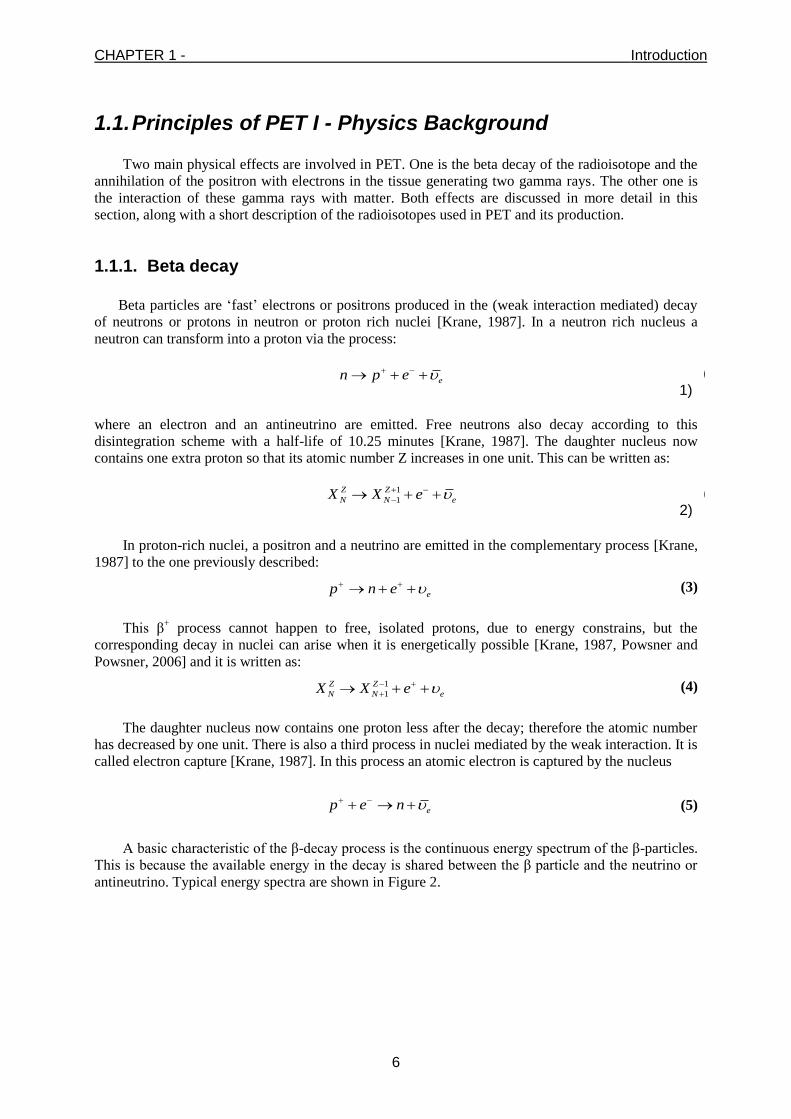
1.1.1. Beta decay
Beta particles are ‘fast’ electrons or positrons produced in the (weak interaction mediated) decay
of neutrons or protons in neutron or proton rich nuclei [Krane, 1987]. In a neutron rich nucleus a
neutron can transform into a proton via the process:
en p e (1)
where an electron and an antineutrino are emitted. Free neutrons also decay according to this
disintegration scheme with a half-life of 10.25 minutes [Krane, 1987]. The daughter nucleus now
contains one extra proton so that its atomic number Z increases in one unit. This can be written as:
1
1
Z Z
N N eX X e
(2)
In proton-rich nuclei, a positron and a neutrino are emitted in the complementary process [Krane,
1987] to the one previously described:
ep n e (3)
This β
+ process cannot happen to free, isolated protons, due to energy constrains, but the
corresponding decay in nuclei can arise when it is energetically possible [Krane, 1987, Powsner and
Powsner, 2006] and it is written as:
1
1
Z Z
N N eX X e
(4)
The daughter nucleus now contains one proton less after the decay; therefore the atomic number
has decreased by one unit. There is also a third process in nuclei mediated by the weak interaction. It is
called electron capture [Krane, 1987]. In this process an atomic electron is captured by the nucleus
ep e n (5)
A basic characteristic of the β-decay process is the continuous energy spectrum of the β-particles.
This is because the available energy in the decay is shared between the β particle and the neutrino or
antineutrino. Typical energy spectra are shown in Figure 2.
CHAPTER 1 - Introduction
7
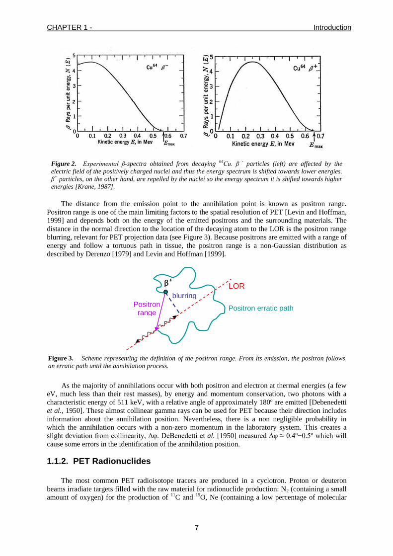
Figure 2. Experimental β-spectra obtained from decaying 64
Cu. β -
particles (left) are affected by the
electric field of the positively charged nuclei and thus the energy spectrum is shifted towards lower energies.
β+ particles, on the other hand, are repelled by the nuclei so the energy spectrum it is shifted towards higher
energies [Krane, 1987].
The distance from the emission point to the annihilation point is known as positron range.
Positron range is one of the main limiting factors to the spatial resolution of PET [Levin and Hoffman,
1999] and depends both on the energy of the emitted positrons and the surrounding materials. The
distance in the normal direction to the location of the decaying atom to the LOR is the positron range
blurring, relevant for PET projection data (see Figure 3). Because positrons are emitted with a range of
energy and follow a tortuous path in tissue, the positron range is a non-Gaussian distribution as
described by Derenzo [1979] and Levin and Hoffman [1999].
Figure 3. Scheme representing the definition of the positron range. From its emission, the positron follows
an erratic path until the annihilation process.
As the majority of annihilations occur with both positron and electron at thermal energies (a few
eV, much less than their rest masses), by energy and momentum conservation, two photons with a
characteristic energy of 511 keV, with a relative angle of approximately 180º are emitted [Debenedetti
et al., 1950]. These almost collinear gamma rays can be used for PET because their direction includes
information about the annihilation position. Nevertheless, there is a non negligible probability in
which the annihilation occurs with a non-zero momentum in the laboratory system. This creates a
slight deviation from collinearity, Δφ. DeBenedetti et al. [1950] measured Δφ ≈ 0.4º−0.5º which will
cause some errors in the identification of the annihilation position.
1.1.2. PET Radionuclides
The most common PET radioisotope tracers are produced in a cyclotron. Proton or deuteron
beams irradiate targets filled with the raw material for radionuclide production: N2 (containing a small
amount of oxygen) for the production of 11
C and 15
O, Ne (containing a low percentage of molecular
LOR +
blurring
Positron erratic path Positron
range

CHAPTER 1 - Introduction
8
fluorine) and 18
O enriched water for the production of 18
F [Stöcklin and Pike, 1993].
There are other isotopes like 82
Rb, 68
Ga which are obtained from generators. These generators
contain relatively long-life mother isotopes, producing the desired isotopes as a result of their decay
process. The separation of the daughter nuclei is made through a chemical processes.
The choice of the radionuclide is imposed by its physical and chemical characteristics and its
availability [Raichle, 1983]. Table 1 lists the most frequently used positron emitting radionuclides
with some of their physical characteristics. The positron energy and its resulting range in water are
inversely correlated with the PET image resolution obtained, especially when using high resolution
PET for small animal imaging. Before application to the patient, the tracer must be tested for
radionuclidic, radiochemical, chemical, and pharmaceutical quality, as well as for sterility. Details on
the quality control of radiopharmaceuticals can be found for example in [Stöcklin and Pike, 1993].
Table 1. Physical properties of positron emitters. (Adapted from [Bailey, 2005] and [Cherry et al., 2003]).
Radionuclide Half-life (min) Production Range in water (mm) Max.
Emission energy (MeV) Max Mean
11C 20.4 cyclotron 4.1 1.1 0.959
13N 9.97 cyclotron 5.1 1.5 1.197
15O 2.03 cyclotron 7.3 2.5 1.738
18F 109.8 cyclotron 2.4 0.6 0.633
82Rb 1.25 generator 14.1 5.9 3.400
68Ga
68 generator 8.9 2.9 1.899
1.1.3. Interaction of gamma radiation with matter
When a monoenergetic gamma beam with intensity I0 passes through matter, the most relevant
interaction occurs with the electrons of the material. As a result of these interactions, some gamma
rays will be removed out of the incident beam by either photoelectric absorption (absorption
coefficient τ), Compton or Rayleigh effects (absorption coefficient σ), or pair production (absorption
coefficient κ) [Knoll, 2000]. An overall absorption coefficient µ results from these three individual
absorption coefficients:
(6)
Thus, the overall absorption can be described by:
0
xI I e (7)
where I0 is the incident and I the resulting intensity after crossing a distance x of material.
CHAPTER 1 - Introduction
9
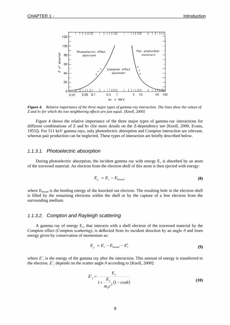
Figure 4. Relative importance of the three major types of gamma-ray interaction. The lines show the values of
Z and hν for which the two neighboring effects are just equal. [Knoll, 2000]
Figure 4 shows the relative importance of the three major types of gamma-ray interactions for
different combinations of Z and hν (for more details on the Z-dependency see [Knoll, 2000, Evans,
1955]). For 511 keV gamma rays, only photoelectric absorption and Compton interaction are relevant,
whereas pair production can be neglected. These types of interaction are briefly described below.
1.1.3.1. Photoelectric absorption
During photoelectric absorption, the incident gamma ray with energy Eγ is absorbed by an atom
of the traversed material. An electron from the electron shell of this atom is then ejected with energy:
boundeE E E
(8)
where Ebound is the binding energy of the knocked out electron. The resulting hole in the electron shell
is filled by the remaining electrons within the shell or by the capture of a free electron from the
surrounding medium.
1.1.3.2. Compton and Rayleigh scattering
A gamma ray of energy Eγ, that interacts with a shell electron of the traversed material by the
Compton effect (Compton scattering), is deflected from its incident direction by an angle θ and loses
energy given by conservation of momentum as:
boundeE E E E
(9)
where E’γ is the energy of the gamma ray after the interaction. This amount of energy is transferred to
the electron. E’γ depends on the scatter angle θ according to [Knoll, 2000]:
cos11
'
2cm
E
EE
e
(10)

CHAPTER 1 - Introduction
10
mec2 being the rest-mass energy of the electron (511 keV). The maximum energy transferred to the
electron occurs when the scattering angle θ = π:
2
2,max
2
1 2
e
ee
E m cE E
E m c
(11)
This gives rise to the Compton edge in the energy spectrum of monoenergetic gamma rays as
seen in detectors of finite size [Knoll, 2000].
When elastic scattering occurs, the incident photon is scattered without ionizations or other
energy losses in excitations of the internal states of the constituents of the material. This process is
known as Rayleigh scatter.
1.1.3.3. Pair production
The energy threshold for pair production
e e (12)
is 2×511 keV = 1.022 MeV. This interaction can only take place in the presence of a nucleus to pick
up recoiling energy and momentum so that energy-momentum conservation can be verified.
Additional energy of the gamma ray will be converted into kinetic energy of the electron, positron and
recoiling partner. As this latter is usually a relatively heavy nucleus, its recoiling energy can be
neglected. Both electrons and positrons produced will undergo interactions with matter, and
additionally these positrons will finally produce annihilation radiation at the end of their paths.
CHAPTER 1 - Introduction
11
1.2. Principles of PET II - Detectors
Detection systems are key components of any imaging system, and an understanding of their
properties is important for establishing appropriate operating criteria or designing schemes.
Scintillation detectors are widely used as radiation detectors in PET imaging. They are very fast, can
have high stopping power and exhibit low electronic noise. A scintillation detector primarily consists
of a crystal that produces scintillation light after interaction with radiation, and a photodetector that
converts the scintillation light into an electrical signal [Wernick and Aarsvold, 2004, Melcher, 2000].
This section primarily discusses the scintillation detector components and design considerations.
1.2.1. Scintillators
Gamma rays can be detected with scintillators, which produce scintillation photons in the visible
and ultraviolet range of wavelengths (100 - 800 nm). As discussed in the previous section, only
photoelectric absorption and Compton scattering are relevant interaction mechanisms for detecting 511
keV gamma photons [Knoll, 2000]. During a photoelectric absorption, the entire energy of the gamma
photon is converted to the release of a photoelectron, a knock-on electron. This electron then excites
higher energy states of the crystal lattice, which decay by emitting lower energy scintillation photons.
During Compton scatter, only part of the energy of the gamma photon is converted to the knock-on
electron. The rest of the energy is taken by the scattered, ‘degraded’ photon. This scattered photon in
turn can produce additional scintillation centers by the Compton and photoelectric effect. Compton
scattering inside the scintillation crystal can thus produce various scintillation centers. This position
blurring affects the position determination. Unlike Compton scatter, the photoelectric effect produces
a single scintillation center and is the preferred interaction process. The photoelectric cross section p
is a function of the density and of the effective atomic number Zeff of the crystal. The photoelectric
cross section is proportional to (Zeff)x, with the power x varying with gamma-ray energy between 3
and 4, typically. In contrast, the Compton cross section is linearly related to the electron density, and
thus proportional to [Eijk, 2002].
A scintillator should thus have a high density for a high absorption probability and a high atomic
number for a large fraction of photons undergoing photoelectric absorption. These two requirements
are commonly parametrized as the attenuation length 1/µ (the distance where the probability that a
particle has not been absorbed drops to 1/e) and photoelectric absorption probability PE or
photofraction, defined as the probability that a gamma photon interacts by the photoelectric effect PE
= 100 [p /(p + c)]
High light yield (number of emitted scintillation photons per MeV absorbed energy) is another
important requirement for PET. A large number of detected scintillation photons Nph imply a better
energy, timing and position resolution. This is because photon counting is dominated by Poisson
statistics, such that the relative statistical spread is proportional to phN1 .
Associated with the light yield requirement is a high light collection efficiency of the crystal, such
that a large fraction of the emitted scintillation photons are detected. Optical self-absorption of the
scintillation photons should therefore be minimal. Furthermore, the scintillator can be surrounded by a
reflector at all surfaces except that at which the photosensor is located, to recapture the light that
would otherwise escape from the crystal. Also, the emission spectrum should overlap with the spectral
sensitivity of the photodetector. It is further desirable that the light output is proportional to the
deposited energy. If this would not be the case, the light output would be different for a full 511 keV
energy absorption by a single photoelectric effect, compared to a full energy absorption by multiple,
lower energy, Compton interactions. This would broaden the full energy peak.
CHAPTER 1 - Introduction
12
The time structure of the light emitted by scintillators can often be approximated by [Ljungberg et
al., 1998]:
0( )RISEFALL tt
FALL RISE
e eN t N
(13)
where N(t) is here the number of photons emitted by the scintillators at time t, N0 is the total number of
photons emitted, and τFALL and τRISE are fall and rise constants of the scintillator.
A fast decay time allows a high count rate performance of the detector. This is especially
important for 3D-mode PET, where high counting rates exist and the system sensitivity will be limited
by pulse pile-up (see section 1.3.7) if slow scintillators are used. Additionally, a fast decay time (as
well as a high light yield) implies a large initial scintillation photon emission rate N0. The rise time,
τRISE, is associated with the luminescence process in scintillators. It should be fast enough to allow a
short coincidence time window to limit the amount of random coincidences (see section 1.3.4). Like a
fast decay time, a fast rise time is associated with a large initial scintillation photon emission rate N0,
and thus a high timing resolution can be obtained for TOF-PET (PET with time-of-flight).
Scintillator materials can be organic-based (liquid or plastic) or inorganic. Organic scintillators
are generally fast, but have a low light yield. Inorganic scintillators have a higher light yield, but are
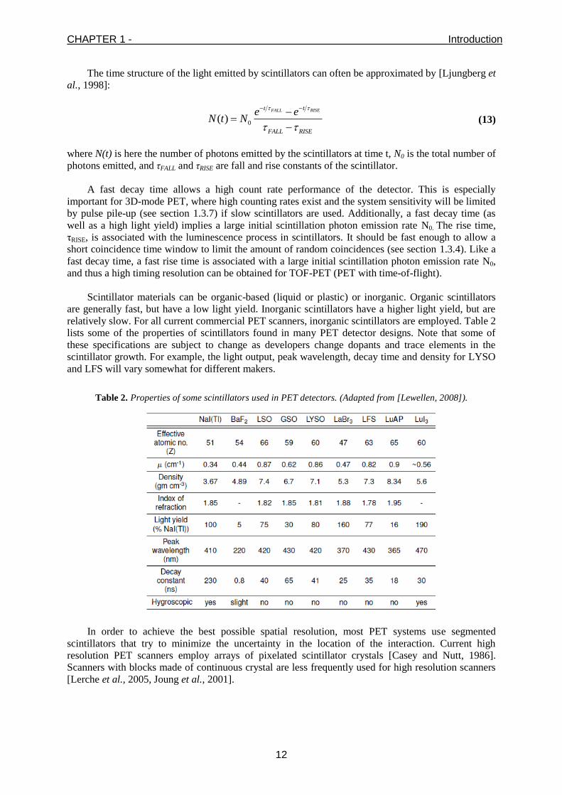
relatively slow. For all current commercial PET scanners, inorganic scintillators are employed. Table 2
lists some of the properties of scintillators found in many PET detector designs. Note that some of
these specifications are subject to change as developers change dopants and trace elements in the
scintillator growth. For example, the light output, peak wavelength, decay time and density for LYSO
and LFS will vary somewhat for different makers.
Table 2. Properties of some scintillators used in PET detectors. (Adapted from [Lewellen, 2008]).
In order to achieve the best possible spatial resolution, most PET systems use segmented
scintillators that try to minimize the uncertainty in the location of the interaction. Current high
resolution PET scanners employ arrays of pixelated scintillator crystals [Casey and Nutt, 1986].
Scanners with blocks made of continuous crystal are less frequently used for high resolution scanners
[Lerche et al., 2005, Joung et al., 2001].
CHAPTER 1 - Introduction
13
1.2.2. Photosensors
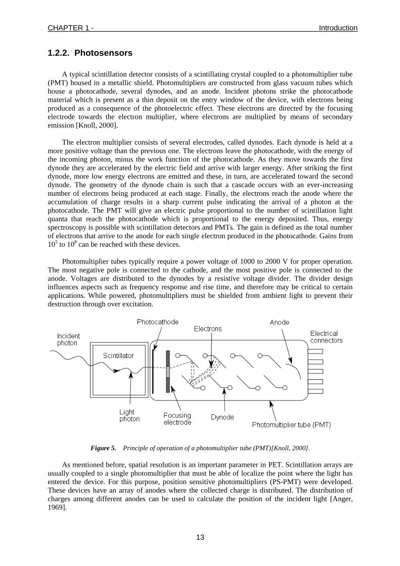
A typical scintillation detector consists of a scintillating crystal coupled to a photomultiplier tube
(PMT) housed in a metallic shield. Photomultipliers are constructed from glass vacuum tubes which
house a photocathode, several dynodes, and an anode. Incident photons strike the photocathode
material which is present as a thin deposit on the entry window of the device, with electrons being
produced as a consequence of the photoelectric effect. These electrons are directed by the focusing
electrode towards the electron multiplier, where electrons are multiplied by means of secondary
emission [Knoll, 2000].
The electron multiplier consists of several electrodes, called dynodes. Each dynode is held at a
more positive voltage than the previous one. The electrons leave the photocathode, with the energy of
the incoming photon, minus the work function of the photocathode. As they move towards the first
dynode they are accelerated by the electric field and arrive with larger energy. After striking the first
dynode, more low energy electrons are emitted and these, in turn, are accelerated toward the second
dynode. The geometry of the dynode chain is such that a cascade occurs with an ever-increasing
number of electrons being produced at each stage. Finally, the electrons reach the anode where the
accumulation of charge results in a sharp current pulse indicating the arrival of a photon at the
photocathode. The PMT will give an electric pulse proportional to the number of scintillation light
quanta that reach the photocathode which is proportional to the energy deposited. Thus, energy
spectroscopy is possible with scintillation detectors and PMTs. The gain is defined as the total number
of electrons that arrive to the anode for each single electron produced in the photocathode. Gains from
105 to 10
8 can be reached with these devices.
Photomultiplier tubes typically require a power voltage of 1000 to 2000 V for proper operation.
The most negative pole is connected to the cathode, and the most positive pole is connected to the
anode. Voltages are distributed to the dynodes by a resistive voltage divider. The divider design
influences aspects such as frequency response and rise time, and therefore may be critical to certain
applications. While powered, photomultipliers must be shielded from ambient light to prevent their
destruction through over excitation.
Figure 5. Principle of operation of a photomultiplier tube (PMT)[Knoll, 2000].
As mentioned before, spatial resolution is an important parameter in PET. Scintillation arrays are
usually coupled to a single photomultiplier that must be able of localize the point where the light has
entered the device. For this purpose, position sensitive photomultipliers (PS-PMT) were developed.
These devices have an array of anodes where the collected charge is distributed. The distribution of
charges among different anodes can be used to calculate the position of the incident light [Anger,
1969].

CHAPTER 1 - Introduction
14
Other devices such as APDs [Pichler et al., 1997], PIN-DIODES or more recently SiPMs are also
being used [Otte et al., 2005, España et al., 2008, España et al., 2010].
1.2.3. Electronics
1.2.3.1. Pulse processing
In order to measure time intervals precisely, the arrival times of different events must be recorded
to achieve optimal time resolution. To obtain good timing signals, Constant Fraction Discriminators
(CFD) may be employed. The output pulse coming from the anode of the PMT, is fed to the input of
the CFD. The principle of operation of a CFD is illustrated in Figure 6.
Figure 6. The formation of the constant-fraction signal [Knoll, 2000].
The CFD is designed to trigger on a certain optimum fraction of the pulse height, thus making the
performance (labeling of the onset of the pulse) of the CFD independent of pulse amplitude2.
Furthermore, leading-edge discriminators (LED) are employed to provide energy selection. Events
with energy below the threshold will not give rise to a signal from the CFD and thus will be excluded.
The events triggered in a detector are fed into coincidence units that test whether each event is
close enough in time to other events from other detectors, so that they can be considered as
coincidence events. The time-of-flight taken by the gamma photons from the positron annihilation
time to the detector is of the order of hundreds of picoseconds, less than the time resolution of most of
PET scanners. However, scanners with time-of-flight (TOF) capabilities have been developed
[Allemand et al., 1980, Mullani et al., 1981, Moszynski et al., 2006]. The time resolution achievable
by the scanner is the result of a convolution of the time resolution of each scintillator, PMT and
2 Assuming all pulses have the same shape. Noise and baseline shifts can prevent this.
CHAPTER 1 - Introduction
15
electronics. It is usually of the order of a few nanoseconds [Knoll, 2000]. However, modern PET
scanners can reach below 500 ps time resolution [Lois et al., 2010, Jakoby et al., 2011].
1.2.3.2. Data acquisition system
Once pulses have passed all discriminators, the amplitude of the signal, that contains the energy
information for the event, must be obtained. All output lines of the PS-PMT that have been triggered
are integrated to obtain the total charge for the energy calculation and the location of the interaction.
This is usually performed by electronic modules that, first, integrate the charge of each output line and
convert the resulting integrated charge into a digital number (ADC conversion) that is transmitted and
stored in a PC. The transmission of this information to the PC may be performed via Ethernet,
fireware, USB, PCI-X or other connections [Lewellen et al., 2001, Lage et al., 2010].
1.2.3.3. Event classification
There are different kinds of events that can be recorded in a PET acquisition:
Single Event (si): A single gamma ray is detected in one of the detectors independently of its
associated second gamma ray.
True Event (T): Two gamma rays that originate from the same e+e
− annihilation and leave the
body without interaction are measured within the same coincidence timing window (τ) (Figure
7a).
However, due to limitations of the detectors used in PET and the possible interaction of the
511 keV photons in the body before they reach the detector, the coincidences measured are
contaminated with undesirable events which includes scattered, random and multiple
coincidences. All these events degrade the quality of the measurement and need to be corrected in
order to produce an image that represents as closely as possible the true radioactivity
concentration under measurement.
Another point to consider is that the vast majority of photons detected by PET scanners are
single events, for which only one of the two annihilation photons is registered. The partner photon
may be on a trajectory such that it does not intersect a detector (most PET scanners provide
relatively modest solid angle coverage around the object), it can be attenuated in the patient or
object placed in the FOV, or the photon may not deposit sufficient energy in a detector to be
registered or may not interact at all. These single events are not accepted by the PET scanner, but
they are responsible for random, multiple coincidence and pile-up events. Because they must still
be processed by the electronics to see if they form part of a coincidence pair, they are an
important contribution to detector dead-time (see sections 1.3.6 and 4.1).
Scatter Event (S): Like a true event, the scatter event originates from a single e+e
− annihilation,
but one (or both) gamma ray undergoes a scatter process while passing through the body. As a
result, the gamma is deflected by an angle θ and its energy decreases according to equation (10).
In a case where this energy is still within the energy window of the PET scanner, the assigned
LOR does not contain any information about the origin of the positron decay (Figure 7e),
resulting in reduction of spatial resolution and image contrast. If not corrected, scattered events
produce a low spatial frequency background that reduces contrast. The distribution of scattered
events depends on the distribution of the radioactivity and the properties of the scattering medium
but it does not depend on the amount of activity administered. In clinical studies, the scatter-to-
true coinicidence ratio ranges from 0.2 to 0.5 for brain and form 0.4 to 2 for abdominal imaging;
in preclinical studies it ranges from 0.1 to 0.6, depending on the size of the object and the
geometry and energy resolution of the PET scanner [Cherry et al., 2003].

CHAPTER 1 - Introduction
16
Figure 7. Illustration of the main coincidence event types: a) true; b) multiple; c) single; d) random and
e) scattered. (Adapted from [Cherry et al., 2003]).
Random Event (R): A random, or accidental, coincidence occurs when two positrons annihilate
and one gamma ray from each annihilation is detected. If the two events occur close enough in
time, then the coincidence electronics will register the event as a coincidence (or a prompt event).
However, such randoms are distributed uniformly in time and only the portion of random events
included in the prompt window contaminates the primary dataset. The assigned LOR again does
not include useful information about the tracer distribution (Figure 7d).
Multiple Event (M): Multiple events result from more than one annihilation and correspond to
the detection, within the same coincidence window, of three or more gamma rays (Figure 7b).
Since there is an ambiguity in deciding which photons make a valid pair, resulting from the same
annihilation, these events are usually discarded by the system.
Pile-up Event (Pu): This kind of event occurs in the detection process if one (or both) gamma
ray is being integrated and an extra gamma ray deposits its energy in the same detector. If the
final energy of the pile-up event is still inside the energy window, it will cause mispositioning of
the true event so the assigned LOR will not contain accurate information about the tracer
distribution.
Prompt Event (P): All coincident events, measured by the coincidence controller, are called
prompt events:
PuRSTP (14)
These events consist of true, scattered, and accidental coincidences where the true
coincidences are the only ones that carry information regarding the spatial distribution of the
radiotracer. It is, therefore, necessary to estimate what fraction of the measured prompt
coincidences arises from scattered and accidental coincidences for each of the LORs [Sorenson
and Phelps, 1987, Tarantola et al., 2003, Bailey, 2005, Valk et al., 2006]

CHAPTER 1 - Introduction
17
1.3. Principles of PET III - Corrections
Quantitative and artifact-free images require applying several corrections to the acquired data.
This section introduces some of the corrections that are commonly applied to PET acquisitions.
1.3.1. Decay
Correcting for decay is often required in procedures involving radioactivity. During a study, the
tracer activity decreases due to radioactive decay of the radionuclide. Therefore, it is necessary to
scale the acquired data by a decay correction factor, Di, which can be calculated as follows [Bailey,
2005]:
The number (N) of counts measured during the acquisition time Δti is:
00( ) 1
i i i ii i
i i
t t t tt tt
t t
AN A t A e e e
(15)
with Δti the duration of the frame that was started at time ti, A0 the initial activity and the decay
constant. If Ai is the mean tracer activity during frame i, we can also write:
i iN A t
(16)
Using (15) and (16) we can obtain:
0 i iA A D (17)
where Di is the decay correction factor:
1
i
i
t
ii t
t eD
e
(18)
This correction factor depends on the duration of the frame, Δti, and the decay constant of the
isotope. This information is usually stored in acquisition files.
1.3.2. Attenuation
Annihilation photons in PET are subject to attenuation as they travel through the imaged object
reducing the number of photons detected in each line of response (LOR). If the anatomical properties
of the object/subject are known, the measurement along each line of response can be corrected for this
attenuation effect [Huang et al., 1979]. A coincidence event requires the simultaneous detection of
both photons coming from the annihilation of a positron. If either photon is absorbed within the body
or scattered out of the field of view, the coincidence will be lost. For this reason, the probability of
detection depends on the combined path of both photons. Since the total path length is the same for all
sources lying on the line that joins two detectors, the probability of attenuation is the same for all such
sources, independently on the source position.
Therefore, the problem of correcting for photon attenuation within the body is equivalent to the
determination of the probability of attenuation for all sources lying along every line of response
CHAPTER 1 - Introduction
18
[Bailey, 2005]. The probability of attenuation for each LOR can be determined by using an external
(transmission) source. With the advent of dual modality scanners capable of acquiring PET and CT
data during the same imaging session, there has been considerable effort put into the development of
methods to employ CT data for PET attenuation correction.
A more detailed description of this correction is depicted in chapter 4 (section 4.3).
1.3.3. Scatter
When a positron annihilates in the body, there is a finite probability that one or both of the
annihilation photons scatter in the body or in the detector itself. At the energy of annihilation photons
(511 keV), the most likely type of interaction is Compton scattering. As it was mentioned in section
1.2.3.3, since the scattered LOR is no longer collinear with the annihilation point, such events degrade
the quality of PET image. Indeed, except for high energy resolution detectors (CZT, HPGe, Si(Li),
BrLa(Ce)) [Vaska et al., 2005, Cooper et al., 2007], scattered coincidences are not easily
discriminated from unscattered ones, solely based on their energy, and thus may significantly degrade
both image quality (due to loss of contrast) and quantitative accuracy [Wirth, 1989]. The fraction of
accepted coincidences which have undergone Compton scattering prior to detection, is named as the
scatter fraction and its magnitude depends on several factors, including size and density of the
scattering medium, geometry of the PET scanner and width of the energy acceptance window. There
are several characteristics of scattered coincidences which can be exploited to estimate their
distribution (and potentially correct for them) in the measured data [Bailey, 2005]:
LORs recorded outside object boundaries can only be explained by scatter in the
object, assuming that random coincidences (see next subsection) have been subtracted.
The distribution of scatter counts is very smooth, i.e., it contains mainly low spatial
frequencies.
The region of the coincidence energy spectrum below the photopeak has a large
contribution from scattered events.
Scattered coincidences that fall within the photopeak window are mainly due to
photons that have scattered only once.
These various characteristics have given rise to a wide variety of approaches for estimating and
correcting scattered coincidences in PET data [Bailey and Meikle, 1994, Levin et al., 1995, Cherry et
al., 1993].
1.3.4. Random coincidences
As explained in section 1.2.3.3, random coincidences arise when two unrelated photons are
detected in opposing detectors, close enough in time to be accepted by the time-window criteria that
the system employs to identify coincidences. Random coincidences add uncorrelated background
counts to PET images and hence decrease image contrast, if no correcting measures are taken [Bailey,
2005].
The number of random coincidences detected can be reduced by choosing the scanner geometry
so that the field of view (FOV) for single events is reduced [Badawi et al., 2000] or by reducing as
much as possible the time coincidence window of the system. The noise introduced by random
coincidences can also be reduced by estimating the number of random counts on each LOR and taking
this estimation into account during reconstruction. The number of random coincidences on a particular
LOR can be estimated in different ways [Cooke et al., 1984]. For instance, the rate of random

CHAPTER 1 - Introduction
19
coincidences Rij on a LOR joining two detectors i and j is:
jiij ssR 2 (19)
where si and sj are the uncorrelated singles rates on detectors i and j respectively [Oliver and Rafecas,
2008], and τ is the width of the logic pulses produced when a photon is absorbed in the detector. The
term 2τ is often referred to as the coincidence timing window [Knoll, 2000]. When the single rate is
measured, all correlated and uncorrelated events are detected. Thus, correlated single events, those that
produce true coincidence events, must be substracted from the total singles rate in order to achieve a
more accurate estimation of random coincidences.
Another way of estimating random coincidences employs delayed coincidence measurements. In
this scheme, timing signals from one detector are delayed by a time significantly greater than the time
coincidence window. In this way, all detected coincidences will be uncorrelated and the number of
coincidences found will be a good estimate of the number of random coincidences in the prompt
signal. This resulting estimate is then subtracted from the number of prompt coincidences to yield the
combined number of true and scattered coincidences [Knoll, 2000]. The advantage of this method is
that the delayed channel has identical dead-time (see section 1.3.6) properties to the prompt channel.
The disadvantage is that the statistical quality of the random coincidences estimate is poorer, as Rij, si
and sj are subject to Poisson statistics and Rij may be a significantly smaller quantity than either si or sj
[Casey and Hoffman, 1986].
More information about methods to estimate and correct the effects of random coincidences in
PET studies can be found for example in [Williams et al., 1979, Badawi et al., 1999, Stearns et al.,
2003, Brasse et al., 2005].
1.3.5. Normalization
LORs in PET datasets have different sensitivity due to variations in detector efficiency, solid
angle subtended, etc [Bailey, 2005]. Information on these variations is required for the reconstruction
of quantitative, artifact-free images. Indeed, most algorithms require that these variations are removed
prior to reconstruction. The process of correcting for these effects is usually known as normalization
[Hoffman et al., 1989, Badawi and Marsden, 1999a] .
In a block detector system, detector elements vary in efficiency because of position of the element
in the block, physical variations in the crystal and light guides and variations in the gains of the
photomultiplier tubes or corresponding detector elements. Other causes of differenced sensitivity are
the energy window selected for each crystal element and the time window alignment [Bailey, 2005].
Accurate normalization is essential for good quantitation in PET. Traditional solutions to the
normalization problem include direct [Defrise et al., 1991b, Vicente et al., 2006], component-based
[Hoffman et al., 1989, Casey et al., 1996, Badawi and Marsden, 1999a] or iterative methods
[Hermansen et al., 1997, Bai et al., 2002]. With direct methods, a known source of activity is scanned,
then the normalization factors are estimated as the ratio between the known ideal number of
coincidences and those actually measured [Defrise et al., 1991a]. The main problem with this method
is that it requires the accumulation of a very large number of counts in order to achieve acceptable
statistical accuracy for each LOR. Component-based methods divide the normalization factors into
detector efficiency and spatial distortion correction, intrinsic detector efficiency, geometric factors,
crystal interference, dead-time factors, etc [Badawi and Marsden, 1999a] .

CHAPTER 1 - Introduction
20
1.3.6. Dead-time
PET scanners may be regarded as a series of subsystems, each of which requires a minimum
amount of time to elapse between successive events, for them to be registered as separated. Since
radioactive decay is a random process, there is always a finite probability that successive events will
occur within any minimum time interval, and at high count-rates, the fraction of events falling in this
category can become very significant. The main effect of this phenomenon is a loss of the linear
relationship between the number of coincidence events registered by the PET scanner and the total
activity inside the FOV. The parameter that characterizes the counting behavior of the system at high
event rates is known as dead-time [Knoll, 2000]. The fractional dead-time of a system at a given
count-rate is defined as the ratio of the measured count-rate and the count-rate that would have been
obtained if the system behaved in a linear manner [Casey et al., 1996].
Dead-time correction schemes are usually constructed measuring the live-time (1–fractional dead-
time) for each subsystem. If this is not possible, an analytic model incorporating knowledge of the
system architecture is constructed, and fitted to data from decaying source experiments. The decay
correction scheme then consists of applying a set of measured and modeled correction factors to the
data acquired.
Dead-time models usually treat system dead-time as being separable into two components,
described as paralyzable and non-paralyzable [Knoll, 2000]. The paralyzable component describes the
situation where the system is unable to process events for a fixed amount of time τ3 after each event. If
one event arrives while the system is busy due to a preceding event, the system remains dead for a
further τ seconds from the time of arrival of the second event. The relationship between the measured
event rate m, the actual event rate n, and the dead-time resulting from a single event is given by:
nm ne (20)
In the non-paralyzable case, the system is again rendered dead for a time τ after each event, but
while the system is dead, further events have no effect. For such systems, the measured count rate
tends asymptotically to a limiting value of τ-1 as the actual count-rate increases, and the relationship
between m, n and τ is given by [Knoll, 2000]:
1
nm
n
(21)
1.3.7. Pile-up
As it was mentioned before, pulse pile-up occurs when a photon deposits energy in the detector
crystal while the signal from the previous event is still being integrated. Pile-up events cause two types
of errors in PET data. The first one occurs when the pile-up event provides a large enough signal to
fall outside the energy window and the event is lost. Under this situation, deadtime corrections will be
required for quantitative measurement. The second error is interaction mispositioning. In detection
systems, which employ a 2-D matrix of crystals and analog logic to identify the crystal of interaction,
the scintillation photons from all crystals are processed as a single event, and for pile-up events the
apparent location of the interaction results from an average of the crystals that absorbed radiation. If
these events are not rejected, they will cause mispositioning of valid coincidence events. This will
cause loss of resolution and contrast in the image, and a transfer of counts between image planes,
leading to loss of counts in the originating plane and additional background events in the destination
plane [Germano and Hoffman, 1990, Badawi and Marsden, 1999b].
For more information about pile-up and dead-time corrections see chapter 4, section 4.1.
3 Although we use the same notation ‘’ to refer to dead-time and coincidence time window, these two
parameters have totally different meaning, as the reader can figure out from the explanation above.

CHAPTER 1 - Introduction
21
1.4. Monte Carlo Simulations
Monte Carlo simulation methods can be described as statistical methods that use random numbers
as a base to model problems involving stochastic processes [Kalos and Whitlock, 1986]. The name of
the technique was chosen during the World War II Manhattan Project due to the close connection to
games of chance and the location of the famous casino in Monte Carlo. The general concept of Monte
Carlo simulation is to create a model, as similar as possible to the real system and to simulate
interactions with that system based on a priori known probabilities of occurrence through random
sampling of Probability Density Functions (PDFs).
Due to the stochastic nature of radiation emission and detection processes, the Monte Carlo
method is particularly interesting for medical physics in areas such as radiotherapy, radiation
protection and nuclear medicine [Andreo, 1991]. In fact, this simulation technique is nowadays an
essential research tool in nuclear medicine to study the response of imaging systems, like PET and
SPECT (Single Photon Emission Computer Tomography) scanners, predicting the performance of new
detectors and optimizing their design [Zaidi, 1999]. In addition, Monte Carlo data is currently essential
for the development, validation and comparative evaluation of image reconstruction techniques and for
the assessment of correction methods such as photon attenuation and scattering. One of the advantages
of Monte Carlo simulations is the possibility to change different parameters and to investigate the
effects of such modifications on the performance of scanners, allowing testing several detection
configurations that may be impracticable using an experimental approach. Following the development
of more powerful computing systems, Monte Carlo has recently been used to produce simulation data
that allows to anticipate the lesion detectability performance of imaging systems under development as
well as to calculate the system matrix for image reconstruction algorithms, as an alternative to
analytical models.
The success of this approach is due to the ability of Monte Carlo techniques to accurately
describe the physics of the interaction of particles with matter by using pseudo–random number
generators, and rules to sample probability distributions and cross–sections to determine the
interaction probability of particles traveling through a given material. When simulating photon
interactions, the partial and total cross section data (based on the material constitution) represent such
information and are used to calculate the path length and type of interaction for this particle.
Afterwards, the PDFs are sampled by predefined sampling rules using randomly generated numbers.
The energy of such a photon can be dissipated along its path or the photon can cross all scattering and
attenuating media to reach the detector where a new PDF sampling decides whether it should be
accounted for in the scoring region or be discarded [Zaidi, 1999, Buvat and Castiglioni, 2002].
A detailed description of the general principles and applications of the Monte Carlo method can
be found in [Andreo, 1991, Ljungberg et al., 1998, Zaidi, 1999, Zaidi and Sgouros, 2003, Zaidi, 2006].
CHAPTER 1 - Introduction
22
1.4.1. Random numbers and probability distribution function
Monte Carlo simulations employ random numbers. A sequence of random numbers is such that it
is impossible to predict which will be the next number in the sequence. Sequences of perfectly random
numbers are almost impossible to generate in a computer, by definition. Instead, pseudo-random
numbers are employed. These pseudo-random numbers are generated by an algorithm that produces
sequences of reasonably unpredictable appearance and with very long repetition cycles. These
algorithms use a seed or initial number as a starting point for the generation of the sequence. Two
sequences will be identical if they are generated from the same seed and algorithm and therefore,
different seeds must be used in each simulation. In addition, these sequences of random numbers are
often built so that they produce random variables that follow an uniform distribution in a specific
range of values, that is, the probability of appearance of any number in the interval would be the same
[Kalos and Whitlock, 1986].
Most programming languages include algorithms to generate sequences of random numbers
uniformly distributed in the interval (0, 1). These are used as the basis for the generation of more
complex distributions suitable for Monte Carlo methods. In what follows we introduce a few statistical
definitions that will be useful for Monte Carlo methods.
The mentioned probability distribution function (PDF) of a continuous variable x (p(x)) is the
function that contains the probability for x taking a specific value. This function must be positive and
normalized to unity in a range of values (xmin, xmax) [Ljungberg et al., 1998].
max
min
0 1x
xp x p x dx
(22)
The cumulative distribution function (CDF) of a variable x is the function that contains the
probability that the value of the random variable falls within a particular interval [xmin, x]. It is
therefore a non-decreasing function from P(xmin)=0 to P(xmax)=1[Ljungberg et al., 1998].
min
x
xx p x dx (23)
The first ingredient of a Monte Carlo calculation is the numerical sampling of random variables
with specified PDFs. Different techniques to generate random values of a variable x, distributed in the
interval (xmin, xmax) according to a given PDF, p(x), are explained in more detail for instance in
[Sempau et al., 2003a].
1.4.2. Monte Carlo Packages for Nuclear Medicine
Several Monte Carlo computer codes for the simulation of radiation transport are available in the
public domain. The majority of Monte Carlo codes were initially designed for high energy physics
experiments or nuclear physics that later found applications also outside their original domain. For that
reason, there is a large community of researchers continuously maintaining and improving these codes
as well as contributing to their validation.
Currently there are many Monte Carlo simulation packages with different characteristics, suitable
for either PET or SPECT processes, at different levels of reliability. Accurate and versatile general-
purpose simulation packages such as EGS4 [Rogers, 1984], MCNP [Briesmeister, 1993], and most
recently PENELOPE [Baró et al., 1995] and Geant4 [Agostinelli, 2003] have been made available.
These latter packages require a lot of expertise in order to model emission tomography configurations.
Further, SimSET [Harrison et al., 1993], GATE [Jan et al., 2004b], Eidolon [Zaidi and Scheurer,
1999], PETSIM [Thompson et al., 1992b], PeneloPET [España et al., 2009], and GAMOS [Arce et al.,

CHAPTER 1 - Introduction
23
2008] are powerful simulation codes for specific applications in PET and SPECT. Nowadays, SimSET
and GATE are probably the most extensively used [Barret et al., 2005, Du et al., 2002, Lazaro et al.,
2004, Chen et al., 2006]. Table 3 shows the principal features of these Monte Carlo codes.
Table 3. Main features of PET Monte Carlo codes. Voxelized attenuation body and activity distributions are
employed to define very complex geometries. Simulation of positron range and non-collinearity is mandatory to
achieve realistic results. If pixelated detector capability is included, the reflector material placed among crystals
can be considered. Random coincidences are very important when simulating high count rates. Some of the
codes have been validated against experimental data.
Reference Voxelized att / act distrib.
Positron Range / Non-
collinearity
Pixelated Detectors
Randoms
Validated
PETSIM [Thompson et
al., 1992b] No Yes Yes Yes No
GATE [Jan et al.,
2004b] Yes Yes Yes Yes Yes
Eidolon [Zaidi and
Scheurer, 1999] Yes Yes Yes No No
SimSET [Harrison et al.,
1993] Yes Yes No No Yes
PeneloPET [España et al.,
2009], No / Yes Yes Yes Yes Yes

CHAPTER 1 - Introduction
24
1.5. Basics of Image Reconstruction
Tomographic images are 2D representations of structures lying within a selected plane in a 3D
object. Tomography projective systems use detectors placed (or rotated) around the object to acquire
many angular views (also known as projections) of a certain property of the object under study.
Mathematical algorithms are then used to reconstruct the object.
Tomography image reconstruction is a problem that has attracted a lot of attention in the last forty
years producing numerous reconstruction schemes. There are two basic approaches to image
reconstruction. One approach is analytic in nature and utilizes the mathematics of computed
tomography that relates line integral measurements to the activity distribution in the object. These
algorithms have a variety of names, including Fourier reconstruction and filtered backprojection
(FBP). The second approach is to use iterative methods that model the data collection process in a PET
scanner and attempt, in a series of successive iterations, to find the image that is most consistent with
the measured data. Figure 8 shows a possible classification of the reconstruction algorithms based on
their mathematical foundation. In this section, the main features of these methods are briefly described
along with different methods to sort PET data.
Figure 8. Classification of image reconstruction algorithms [Fessler, 2008].
Currently, the most commonly used image reconstruction methods are FBP and OSEM. They
have been the ones employed in this thesis and will be explained in more detail in the following
sections.
1.5.1. Data organization
1.5.1.1. List-mode data
The quantity of interest in PET is the 3D spatial distribution of a tracer inside the body, f (x,y,z).
The raw data collected by a PET scanner are a list of ‘coincidence events’, representing near-
simultaneous detection of annihilation photons by a pair of detectors. Each coincidence event defines a
line in space along which the positron emission occurred, referred to as line of response (LOR), as it
was introduced before.
One way to store the measured coincidence events for further processing is to write the
information from prompt events in order of occurrence in the acquisition system. An event packet
would include crystal number, energy, positioning, etc. In addition, gantry information (e.g. count rate

CHAPTER 1 - Introduction
25
and time information) as well as external data (e.g. gating and patient motion information) can be
included into the list-mode stream in the form of tag words [Byme, 2001, Parra and Barrett, 1998].
The event packets stored are processed afterwards and eventually transformed into sinogram
datasets (see section 1.5.1.2) or LOR histograms [Kadrmas, 2004], while the timing information is
analyzed so that the dataset can be split into different time frames.
1.5.1.2. Projections and sinograms
Considering the two dimensional case, a projection is defined as the number of counts in a set of
parallel LORs at a specific angle [Bailey, 2005]
p s, f x, y dyr
(24)
where f (x,y) is a two-dimensional representation of the activity distribution, s is the radial coordinate,
and yr is the transversal direction coordinate. Projections from all angles can be arranged in a matrix.
Because a point source will describe a sinusoidal trajectory in this matrix representation (see Figure 9),
the matrix is called a sinogram [Bailey, 2005, Bendriem and Townsend, 1998]. Sinograms are the
basis of most of the image reconstruction schemes [Bendriem and Townsend, 1998].
Figure 9. The projections of a point source at different angles (right) are represented with a sine curve in
a sinogram representation the data acquired [Bailey, 2005].
1.5.1.3. Data rebinning
Rebinning algorithms allow for the sorting of data from oblique sinograms of a 3D dataset into
the corresponding planes of a 2D dataset. This way, it is possible to reconstruct a 3D dataset with
conventional 2D reconstruction schemes, while maintaining the sensitivity of 3D acquisitions. Mainly
two approaches are used in clinical routine: single slice rebinning (SSRB) [Daube-Witherspoon and
Muehllehner, 1987] and Fourier rebinning (FORE) [Defrise et al., 1997].
CHAPTER 1 - Introduction
26
Single-Slice Rebinning (SSRB)
This approximate algorithm [Daube-Witherspoon and Muehllehner, 1987] is based on the
assumption that each oblique LOR measured crosses only a single transaxial section within the support
of tracer distribution. SSRB defines the rebinned sinograms by [Bailey, 2005]:
max
maxmax
1, , , , ,
2 ,ssrb sp s z p s z d
s z
(25)
max2 2
min ,, arctan
d
z L zs z
R s
(26)
where θmax is the maximum axial aperture for a LOR at a distance s from the axis in slice z, Rd is the
scanner radius, and L the number of transaxial sections sampled. The algorithm is exact for tracer
distributions which are linear in z. For realistic distributions, the accuracy of the approximation will
decrease with increased transaxial FOV radius and with increased θmax. Axial blurring and transaxial
distortions, which increase with the distance to the axis of the scanner and θ, are the main drawbacks
of the SSRB approximation.
Fourier rebinning (FORE)
The approximate Fourier rebinning algorithm [Defrise et al., 1997] is more accurate than the
SSRB algorithm and extends the range of 3D PET studies that can be processed using rebinning
algorithms. The main characteristic of FORE is that it proceeds via a 2D Fourier transform of each
oblique sinogram. Rebinning is based on the following relation between Fourier transforms of oblique
and direct sinograms [Bailey, 2005]
,2/tankz,k,P0,z,k,P ss (27)
where k is the azimuthal Fourier index. The FORE method slightly amplifies the statistical noise, as
compared to SSRB, but results in significantly less azimuthal distortion.
1.5.2. Analytical methods
The central-section theorem states that, in a 2D slice, the Fourier transform of a one-dimensional
projection is equivalent to a section, or profile, at the same angle through the center of the two-
dimensional Fourier transform of the object [Kak and Slaney, 1988]. Figure 10 shows a pictorial
description of the central-section theorem, where F1{ p(s,) } is the one–dimensional Fourier
transform of a projection, F2{ f (x,y) } is the two-dimensional Fourier transform of the image, and υx is
the Fourier space conjugate of x. The central-section theorem indicates that if we know P( S ,) at all
angles, then we can fill in values for F( x , y ). The inverse two dimensional Fourier transform of
F( x , y ) will give f (x,y).
P s , 1 p s, 2 f x, y F x ,y
(28)
Backprojection is the adjoint operation to the forward projection process that yields the

CHAPTER 1 - Introduction
27
projections of the object. Figure 11 shows the backprojection along a fixed angle . Conceptually,
backprojection can be described as placing a value of p(s,) back into an image array along the
appropriate LOR but, since the knowledge of where the values came from was lost in the projection
step, a constant value is placed into all elements along the LOR [Henkin et al., 2006].
Figure 10. Pictorial illustration of the two-dimensional central-section theorem, showing the equivalency
between the one-dimensional Fourier transform (top right) of a projection at angle (top left) and the central-
section at the same angle (bottom left) through the two-dimensional Fourier transform of the object (bottom
right) [Bailey, 2005].
A simple backprojection of all the collected projections is not enough to obtain a good image due
to the oversampling in the center of the Fourier space. This oversampling in the center of Fourier
space needs to be filtered in order to have equal sampling throughout the Fourier space. Basically, the
Fourier transform of the backprojected image must be filtered with a ramp filter 2
y
2
x . This
cone filter accentuates the values at the edge of the Fourier space and reduces the ones at the center.
Figure 11. Backprojection, b(x,y;), into an image reconstruction array of all values of p(s,) for a fixed value
of [Henkin et al., 2006].
CHAPTER 1 - Introduction
28
The filtered-backprojection (FBP) reconstruction algorithm is the most well-known method for
image reconstruction which applies the concept of backprojection and filtering explained before.
Within FBP, the general expression employed to calculate the source distribution from projection data
is [Herman, 1980]:
1
1 1
0
, ,sf x y p s d
(29)
In order to reduce the noise in the images, additional filters like Hanning or Butterworth are
commonly used [Cherry et al., 2003].
The advantages of FBP consist on its linearity, reproducibility, relatively easy implementation,
and low computational cost. As it is considered the standard reconstruction method, it employed in to
compair scanners [Goertzen et al., 2012]. However, it has some important disadvantages in PET: it
assumes Gaussian, instead of Poisson noise, therefore may create streak artifacts [Cherry et al., 2003],
it does not allow resolution recovery as iterative methods do. Additionally it may produce images with
spurious negative values. In this thesis FBP has been used at times to evaluate the performance of
different scanners.
1.5.3. Iterative methods
The imaging process of estimating the y(i) counts on each of the i pair of detectors, from an object
discretized in x(j) voxels, can be described by the operation:
,j
y i A i j x j
(30)
where A(i,j) is the system response matrix (SRM). The vector x(j) corresponds to the voxelized image
and y(i) to the measured data, equivalent to f(x,y) and p(s,) respectively in the analytical
reconstruction framework. Notation has been modified to keep the text congruent with most of the
iterative reconstruction methods in literature.
Each element A(i,j) is defined as the probability of detecting an annihilation event coming from
image voxel j by a detector pair i. This probability depends on factors such as the solid angle
subtended by the voxel to the detector element, the attenuation and scatter in the source volume and
the detector response characteristics.
The forward projection operation just introduced above, estimates the projection data from a
given activity distribution of the source. Backward projection estimates a source volume distribution
of activity from the projection data. The operation corresponds to:
i
)i(y)j,i(A)j(b (31)
where b(j) denotes an element of the backward projection image. Both the forward and backward
projection operations require the knowledge of the SRM [Frese et al., 2001, Rafecas et al., 2004].
Iterative reconstruction algorithms repeatedly use the forward and backward projection operations,
which are the most time-consuming parts of iterative reconstruction programs. Some implementations
trade accuracy for speed by making approximations that neglect some physical processes, such as
positron range, scatter and fractional energy collection at the scintillators or visible light loses in the
detectors [Vaquero et al., 2004, Lee et al., 2000, Yamaya et al., 2003]. This approach simplifies these
operations to gain speed, but this tradeoff often leads to non-optimal images.

CHAPTER 1 - Introduction
29
1.5.3.1. EM-ML
The most widely applied algorithm for finding the maximum-likelihood (ML) estimation of
activity f given the projections p, is the expectation maximization (EM). This was first applied to the
emission tomography problem by Shepp and Vardi [Shepp and Vardi, 1982]. ML, though, is a general
statistical method, formulated to solve many different optimization problems in physics, biology,
economy and others. The EM-ML algorithm can be written as [Herraiz et al., 2006b]:
i
i
'j
it
it1it
)j,i(A
)'j(x)'j,i(A
)i(y)j,i(A
)j(x)j(x (32)
where x
it(j) is the expected value of voxel j at iteration it. The accuracy of the SRM will be extremely
important for the quality of the images resulting from the reconstruction method [Mumcuoglu et al.,
1996].
Usually, iterative algorithms based on ML statistical models assume that the data being
reconstructed retain Poisson statistics [Shepp and Vardi, 1982]. However, to preserve the Poisson
statistical nature of data, it is usually necessary to avoid pre-corrections [Qi et al., 1998] to the data.
Corrections for randoms, scatter and other effects should be incorporated into the reconstruction
procedure itself, rather than being applied as pre-corrections to the data. At times, sophisticated
rebinning strategies are employed to build sinograms into radial and angular sets. This also changes
the statistical distribution of the data, which may no longer be Poisson like [Kadrmas, 2004].
A serious disadvantage of the EM procedure is its slow convergence [Lewittt et al., 1994].
Typically, hundreds of image updates are required. This is due to the fact that the image is updated
only after a full iteration is finished, that is, when all the LORs have been projected and back projected
at least once. In the ordered subset EM (OSEM) algorithm, proposed by [Hudson and Larkin, 1994],
the image is updated more often, which has been shown to reduce the number of necessary iterations
to achieve a convergence equivalent to that of EM:
convergence : Subiterations Iterations Subsets
According to the literature, EM methods have another important drawback: noisy images are
obtained from over-iterated reconstructions, and this is usually attributed to either the fact that there is
no stopping rule in this kind of iterative reconstruction [Johnson, 1987] or to the statistical (noisy)
nature of the detection process and reconstruction method [Bettinardi et al., 2002, Biemond et al.,
1990]. In practice, an image of reasonable quality is obtained after a few iterations [Hudson and
Larkin, 1994].
Several techniques have been proposed to address the noisy nature of the data: filtering the image
either after completion of the reconstruction, during iterations or between them [Slijpen and Beekman,
1999], removal of noise from the data using wavelet based methods [Mair et al., 1996] or smoothing
the image with Gaussian kernels (Sieves method) [Snyder et al., 1987, Liow and Strother, 1991].
Maximum a priori (MAP) algorithms are also widely used [Green, 1990]. MAP adds a priori
information during the reconstruction process, the typical assumption being that due to the inherent
finite resolution of the system the reconstructed image should not have abrupt edges. Thus, MAP
methods apply a penalty function to those voxels which differ too much from their neighbours.
Whether the maximum effective resolution achievable is limited, or even reduced, by the use of these
methods is still an open issue [Alessio et al., 2003]. On the other hand, a proper choice of the

CHAPTER 1 - Introduction
30
reconstruction parameters, such as the number of iterations, the use of an adequate system response
and a smart choice of subsetting, allows high quality images to be obtained by the EM procedure
[Herraiz et al., 2006b].
In this thesis the iterative method has been extensively used because it produces images with
higher quality. Futhermore, a new regularization procedure has been implemented in order to get a
more uniform resolution in the image for certain scanner configurations.

CHAPTER 1 - Introduction
31
1.6. References Agostinelli, S. 2003. GEANT4 - a simulation toolkit. Nucl. Inst. Meth. In Phy. Res. A, 506, 250-303.
Alessio, A., Sauer, K. & Bouman, C. A. 2003. MAP reconstruction from spatially correlated PET data. Nuclear Science,
IEEE Transactions on, 50, 1445-1451.
Allemand, R., Gresset, C. & Vacher, J. 1980. Potential advantages of a Cesium Floride scintillator for time-of-flight
positron camera. J. Nucl. Med., 21, 153-5.
Andreo, P. 1991. Monte Carlo techniques in medical radiation physics. Physics in Medicine and Biology, 36, 861.
Anger, H. O. 1969. Scintillation Camera and Multiplane Tomographic Scanner. Kaku Igaku, 62, 125-48.
Arce, P., Rato, P., Canadas, M. & Lagares, J. I. 2008. GAMOS: A Geant4-based easy and flexible framework for nuclear
medicine applications. In: Nuclear Science Symposium Conference Record, 2008. NSS '08. IEEE, 19-25 Oct. 2008
2008. 3162-3168.
Badawi, R. D., Kohlmyer, S. G., Harrison, R. L., Vannoy, S. D. & Lewellen, T. K. 2000. The effect of camera geometry on
singles flux, scatter fraction and trues and randoms sensitivity for cylindrical 3D PET-a simulation study. Nuclear
Science, IEEE Transactions on, 47, 1228-1232.
Badawi, R. D. & Marsden, P. K. 1999a. Developments in component-based normalization for 3D PET. Physics in
Medicine and Biology, 44, 571.
Badawi, R. D. & Marsden, P. K. 1999b. Self-normalization of emission data in 3D PET. IEEE Transactions on Nuclear
Science, 46, 709-712.
Badawi, R. D., Miller, M. P., Bailey, D. L. & Marsden, P. K. 1999. Randoms variance reduction in 3D PET. Phys Med
Biol, 44, 941-54.
Bai, B., Li, Q., Holdsworth, C. H., Asma, E., Tai, Y. C., Chatziioannou, A. & Leahy, R. M. 2002. Model-based
normalization for iterative 3D PET image reconstruction. Physics in Medicine and Biology, 47, 2773.
Bailey, D. L. 2005. Positron emission tomography: basic sciences, Springer.
Baró, J., Sempau, J., Fernández-Varea, J. M. & Salvat, F. 1995. PENELOPE: An algorithm for Monte Carlo simulation of
the penetration and energy loss of electrons and positrons in matter. Nucl. Inst. Meth. In Phy. Res. B, 100, 31-46.
Barret, O., Carpenter, T. A., Clark, J. C., Ansorge, R. E. & Fryer, T. D. 2005. Monte Carlo simulation and scatter
correction of the GE Advance PET scanner with SimSET and Geant4. Phys. Med. Biol., 50, 4823-40.
Bendriem, B. & Townsend, D. W. 1998. The theory and practice of 3D PET. Kluwer Academic.
Bettinardi, V., Pagani, E., Gilardi, M. C., Alenius, S., Thielemans, K., Teras, M. & Fazio, F. 2002. Implementation and
evaluation of a 3D one-step late reconstruction algorithm for 3D positron emission tomography brain studies using
median root prior. Eur. J. Nucl. Med. Mol. Imaging, 29, 7-18.
Biemond, J., Lagendijk, R. & Mersereau, R. 1990. Iterative methods for image deblurring In: IEEE NSS-MIC, 1990. 856-
883.
Brasse, D., Kinahan, P. E., Lartizien, C., Comtat, C., Casey, M. & Michel, C. 2005. Correction methods for random
coincidences in fully 3D whole-body PET: impact on data and image quality. J Nucl Med, 46, 859-67.
Briesmeister, J. F. 1993. MNCP 4 A, Monte Carlo N-Particle Transport System. Los Alamos, New Mexico: Los Alamos
National Laboratory.
Buvat, I. & Castiglioni, I. 2002. Monte carlo simulations in spet and pet. The quarterly journal of nuclear medicine, 46, 48–
61.
Byme, C. L. 2001. Likelihood maximization for list-mode emission tomographyc image reconstruction. IEEE Trans. Med.
Imaging, 20, 1084-92.
Casey, M. E., Gadagkar, H. & Newport, D. 1996. A component based method for normalization in volume PET. In:
GRANGEAT, P. & AMANS, J. L., eds. Three-Dimensional Image Reconstruction in Radiology and Nuclear Medicine,
1996 Aix-Les-Bains, France. Kluwer Academic, 66-71.
Casey, M. E. & Hoffman, E. J. 1986. Quantitation in positron emission computed tomography: 7. A technique to reduce
noise in accidental coincidence measurements and coincidence efficiency calibration. J Comput Assist Tomogr, 10,
845-50.
Casey, M. E. & Nutt, R. 1986. A Multicrystal Two Dimensional BGO Detector System for Positron Emission
Tomography. IEEE Trans. Nuc. Sci., 33, 460-463.
Cooke, B. E., Evans, A. C., Fanthome, E. O., Alarie, R. & Sendyk, A. M. 1984. Performance Figures and Images from the
Therascan 3128 Positron Emission Tomograph. Nuclear Science, IEEE Transactions on, 31, 640-644.
Cooper, R., Turk, G., Boston, A., Boston, H., Cresswell, J., Mather, A., Nolan, P., Hall, C., Lazarus, I. & Simpson, J. 2007.
Position sensitivity of the first SmartPET HPGe detector. Nuclear Instruments and Methods in Physics Research
Section A: Accelerators, Spectrometers, Detectors and Associated Equipment, 573, 72-75.
Chen, Y., Liu, B., O'Connor, M., Didier, C. S. & Glick, S. J. 2006. Comparison of Scatter/Primary Measurements with
GATE Simulations for X-Ray Spectra in Cone Beam CT Mammography. In: IEEE NSS-MIC, 2006 San Diego.

CHAPTER 1 - Introduction
32
USA, 3909-14.
Cherry, S. R., Sorenson, J. A. & Phelps, M. E. 2003. Physics in nuclear medicine, Saunders.
Daube-Witherspoon, M. E. & Muehllehner, G. 1987. Treatment of axial data in three-dimensional PET. J Nucl Med, 28,
1717-24.
DeBenedetti, S., Cowan, C. E., Konneker, W. R. & Primakoff, H. 1950. On the angular distribution of two-photon
annihilation radiation. Physical Review, 77, 205-212.
Defrise, M., Kinahan, P. E., Townsend, D. W., Michel, C., Sibomana, M. & Newport, D. F. 1997. Exact and approximate
rebinning algorithms for 3-D PET data. Medical Imaging, IEEE Transactions on, 16, 145-158.
Defrise, M., Townsend, D. & Clack, R. 1991a. Favor: a fast reconstruction algorithm for volume imaging in PET. In:
Nuclear Science Symposium and Medical Imaging Conference, 1991., Conference Record of the 1991 IEEE, 2-9
Nov 1991 1991a. 1919-1923 vol.3.
Defrise, M., Townsend, D. W., Bailey, D., Geissbuhler, A. M. C. & Jones, T. 1991b. A normalization technique for 3D
PET data. Physics in Medicine and Biology, 36, 939.
Derenzo, S. E. 1979. Precision measurement of annihilation point spread distributions for medically important positron
emitters. In: 5th Int. Conf. of Positron Annihilation, 1979 Lake Yamanaka, Japan. 819–23.
Du, Y., Frey, E. C., Wang, W. T., Tocharoenchai, C., Baird, W. H. & Tsui, B. M. W. 2002. Combination of MCNP and
SimSET for Monte Carlo simulation of SPECT with medium- and high-energy photons. IEEE Trans. Nuc. Sci., 49,
668-74.
Eijk, C. W. E. v. 2002. Inorganic scintillators in medical imaging. Physics in Medicine and Biology, 47, R85.
España, S., Fraile, L. M., Herraiz, J. L., Udías, J. M., Desco, M. & Vaquero, J. J. 2010. Performance evaluation of SiPM
photodetectors for PET imaging in the presence of magnetic fields. Nuclear Instruments and Methods in Physics
Research Section A: Accelerators, Spectrometers, Detectors and Associated Equipment, 613, 308-316.
España, S., Herraiz, J. L., Vicente, E., Vaquero, J. J., Desco, M. & Udias, J. M. 2009. PeneloPET, a Monte Carlo PET
simulation tool based on PENELOPE: features and validation. Phys Med Biol, 54, 1723-42.
España, S., Tapias, G., Fraile, L. M., Herraiz, J. L., Vicente, E., Udias, J., Desco, M. & Vaquero, J. J. 2008. Performance
evaluation of SiPM detectors for PET imaging in the presence of magnetic fields. In: Nuclear Science Symposium
Conference Record, 2008. NSS '08. IEEE, 19-25 Oct. 2008 2008. 3591-3595.
Fessler, J. A. 2008. Iterative Methods for Image Reconstruction (ISBI Tutorial).
Frese, T., Rouze, N. C., Bouman, C. A., Sauer, K. & Hutchins, G. D. 2001. Quantitative comparison of FBP, EM, and
Bayesian reconstruction algorithms, including the impact of accurate system modeling, for the IndyPET scanner.
In: Nuclear Science Symposium Conference Record, 2001 IEEE, 2001 2001. 1806-1810.
Germano, G. & Hoffman, E. J. 1990. A study of data loss and mispositioning due to pileup in 2-D detectors in PET.
Goertzen, A. L., Bao, Q., Bergeron, M., Blankemeyer, E., Blinder, S., Cañadas, M., Chatziioannou, A. F., Dinelle, K.,
Elhami, E., Jans, H.-S., Lage, E., Lecomte, R., Sossi, V., Surti, S., Tai, Y.-C., Vaquero, J. J., Vicente, E., Williams,
D. A. & Laforest, R. 2012. NEMA NU 4-2008 Comparison of Preclinical PET Imaging Systems. The Journal of
Nuclear Medicine (Accepted).
Green, P. J. 1990. Bayesian reconstructions from emission tomography data using a modified EM algorithm. Medical
Imaging, IEEE Transactions on, 9, 84-93.
Harrison, R. L., Vannoy, S. D., Haynor, D. R., Gillispie, S. B., Kaplan, M. S. & Lewellen, T. K. 1993. Preliminary
Experience With The Photon History Generator Module Of A Public-domain Simulation System For Emission
Tomography. In: Nuclear Science Symposium and Medical Imaging Conference, 1993., 1993 IEEE Conference
Record., 31 Oct-6 Nov 1993 1993. 1154-1158.
Henkin, R. E., Bova, D., Dillehay, G. L. & Karesh, S. M. 2006. Nuclear medicine, Philadelphia, Elsevier Health Sciences.
Herman, G. T. 1980. Image reconstruction from projections: the fundamentals of computerized tomography, Academic
Press.
Hermansen, F., Spinks, T. J., Camici, P. G. & Lammertsma, A. A. 1997. Calculation of single detector efficiencies and
extension of the normalization sinogram in PET. Phys Med Biol, 42, 1143-54.
Herraiz, J. L., España, S., Vaquero, J. J., Desco, M. & Udias, J. M. 2006b. FIRST: Fast Iterative Reconstruction Software
for (PET) tomography. Phys. Med. Biol., 51, 4547-4565.
Hoffman, E. J., Guerrero, T. M., Germano, G., Digby, W. M. & Dahlbom, M. 1989. PET system calibrations and
corrections for quantitative and spatially accurate images. Nuclear Science, IEEE Transactions on, 36, 1108-1112.
Huang, S. C., Hoffman, E. J., Phelps, M. E. & Kuhl, D. E. 1979. Quantitation in positron emission computed tomography:
2. Effects of inaccurate attenuation correction. J Comput Assist Tomogr, 3, 804-14.
Hudson, H. M. & Larkin, R. S. 1994. Accelerated image reconstruction using ordered subsets of projection data. Medical
Imaging, IEEE Transactions on, 13, 601-609.
Jakoby, B. W., Bercier, Y., Conti, M., Casey, M. E., Bendriem, B. & Townsend, D. W. 2011. Physical and clinical
performance of the mCT time-of-flight PET/CT scanner. Phys Med Biol, 56, 2375-89.
Jan, S., Santin, G., Strul, D., Staelens, S., Assie, K., Autret, D., Avner, S., Barbier, R., Bardies, M., Bloomfield, P. M.,

CHAPTER 1 - Introduction
33
Brasse, D., Breton, V., Bruyndonckx, P., Buvat, I., Chatziioannou, A. F., Choi, Y., Chung, Y. H., Comtat, C.,
Donnarieix, D., Ferrer, L., Glick, S. J., Groiselle, C. J., Guez, D., Honore, P. F., Kerhoas-Cavata, S., Kirov, A. S.,
Kohli, V., Koole, M., Krieguer, M., van der Laan, D. J., Lamare, F., Largeron, G., Lartizien, C., Lazaro, D., Maas,
M. C., Maigne, L., Mayet, F., Melot, F., Merheb, C., Pennacchio, E., Perez, J., Pietrzyk, U., Rannou, F. R., Rey, M.,
Schaart, D. R., Schmidtlein, C. R., Simon, L., Song, T. Y., Vieira, J. M., Visvikis, D., Van de Walle, R., Wieers, E.
& Morel, C. 2004b. GATE: a simulation toolkit for PET and SPECT. Phys Med Biol, 49, 4543-61.
Johnson, V. E. 1987. A note on stopping rules in EM-ML reconstructions of ECT images. IEEE Trans. Med. Imaging, 13,
569-71.
Joung, J., Miyaoka, R. S. & Lewellen, T. K. 2001. cMiCE:a high resolution animal PET using continuous LSO with a
statistics based positioning scheme. In: IEEE NSS-MIC, 2001. 1137-1141 vol.2.
Kadrmas, D. J. 2004. LOR-OSEM: statistical PET reconstruction from raw line-of-response histograms. Phys. Med. Biol.,
49, 4731-4744.
Kak, A. C. & Slaney, M. 1988. Principles of Computerized Tomographic Imaging, New York, Society for Industrial
Mathematics.
Kalos, M. H. & Whitlock, P. A. 1986. Monte Carlo Methods, vol. 1, New York, Wiley.
Knoll, G. F. 2000. Radiation detection and measurement / Glenn F. Knoll, New York :, Wiley.
Krane, K. S. 1987. Introductory Nuclear Physics, New York, Wiley.
Lage, E., Tapias, G., Villena, J., Desco, M. & Vaquero, J. J. 2010. Data acquisition electronics for gamma ray emission
tomography using width-modulated leading-edge discriminators. Physics in Medicine and Biology, 55, 4291.
Lazaro, D., Buvat, I., Loudos, G., Strul, D., Santin, G., Giokaris, N. & Donnarieix, D. 2004. Validation of the GATE
Monte Carlo simulation platform for modelling a CsI(Tl) scintillation camera dedicated to small-animal imaging.
Phys. Med. Biol., 49, 271-285.
Lee, J., Vaquero, J. J., Barbosa, F. J., Seidel, J. & Green, M. V. 2000. High performance phoswich detector module for
small animal PET. J. Nucl. Med., 41.
Lerche, C. W., Benlloch, J. M., Sanchez, F., Pavon, N., Escat, B., Gimenez, E. N., Fernandez, M., Torres, I., Gimenez, M.,
Sebastia, A. & Martinez, J. 2005. Depth of γ-ray interaction within continuous crystals from the width of
its scintillation light-distribution. Nuclear Science, IEEE Transactions on, 52, 560-572.
Levin, C. S. & Hoffman, E. J. 1999. Calculation of positron range and its effect on the fundamental limit of positron
emission tomography system spatial resolution. Phys. Med. Biol., 44, 781-799.
Lewellen, T. K. 2008. Recent developments in PET detector technology. Phys Med Biol, 53, R287-317.
Lewellen, T. K., Laymon, C. M., Miyaoka, R. S., Ki Sung, L. & Kinahan, P. E. 2001. Design of a Firewire based data
acquisition system for use in animal PET scanners. In: Nuclear Science Symposium Conference Record, 2001
IEEE, 2001 2001. 1974-1978.
Lewittt, R. M., Muehllehner, G. & Karpt, J. S. 1994. Three-dimensional image reconstruction for PET by multi-slice
rebinning and axial image filtering. Phys Med Biol, 39, 321-39.
Liow, J. S. & Strother, S. C. 1991. Practical tradeoffs between noise, resolution and quantitation, and number of
iterationsfor maximum likelihood reconstructions. IEEE Trans. Med. Imag., 10, 563-571.
Ljungberg, M., Strand, S. E. & King, M. A. 1998. Monte Carlo calculations in nuclear medicine: applications in
diagnostic imaging, Institute of Physics Pub.
Lois, C., Jakoby, B. W., Long, M. J., Hubner, K. F., Barker, D. W., Casey, M. E., Conti, M., Panin, V. Y., Kadrmas, D. J.
& Townsend, D. W. 2010. An assessment of the impact of incorporating time-of-flight information into clinical
PET/CT imaging. J Nucl Med, 51, 237-45.
MacManus, M., Nestle, U., Rosenzweig, K. E., Carrio, I., Messa, C., Belohlavek, O., Danna, M., Inoue, T., Deniaud-
Alexandre, E., Schipani, S., Watanabe, N., Dondi, M. & Jeremic, B. 2009. Use of PET and PET/CT for radiation
therapy planning: IAEA expert report 2006-2007. Radiother Oncol, 91, 85-94.
Mair, B. A., Carroll, R. B. & Anderson, J. M. M. 1996. Filter banks and the EM algorithm. In: Nuclear Science
Symposium, 1996. Conference Record., 1996 IEEE, 2-9 Nov 1996 1996. 1747-1751 vol.3.
Melcher, C. L. 2000. Scintillation crystals for PET. J Nucl Med, 41, 1051-5.
Moszynski, M., Kapusta, M., Nassalski, A., Szczesniak, T., Wolski, D., Eriksson, L. & Melcher, C. L. 2006. New
Prospects for Time-of-Flight PET with LSO Scintillators. IEEE Trans. Nuc. Sci., 53, 2484-8.
Mullani, N. A., Ficke, D. C., Hartz, R., Markham, J. & Wong, G. 1981. System design of a fast PET scanner utilizing time-
of-flight. IEEE Trans. Nuc. Sci., NS-28, 104-7.
Mumcuoglu, E. U., Leahy, R. M. & Cherry, S. R. 1996. Bayesian reconstruction of PET images: methodology and
performance analysis. Phys Med Biol, 41, 1777-807.
Oliver, J. F. & Rafecas, M. 2008. Revisiting the singles rate method for modeling accidental coincidences in PET. In:
Nuclear Science Symposium Conference Record, 2008. NSS '08. IEEE, 19-25 Oct. 2008 2008. 4288-4291.
Otte, A. N., Barral, J., Dogolshein, B., Hose, J., Klemin, S., Lorenz, E., Mirzoyan, R., Popova, E. & Teshima, M. 2005. A
Test of Silicon Photomultipliers as Readout for PET. Nucl.Instrum.Meth.A, 705-715.

CHAPTER 1 - Introduction
34
Papathanassiou, D., Bruna-Muraille, C., Liehn, J. C., Nguyen, T. D. & Cure, H. 2009. Positron Emission Tomography in
oncology: present and future of PET and PET/CT. Crit Rev Oncol Hematol, 72, 239-54.
Parra, L. & Barrett, H. H. 1998. List-mode likelihood: EM algorithm and image quality estimation demonstrated on 2D
PET. IEEE Trans. Med. Imag., 17, 228-35.
Pichler, B., Lorenz, E., Mirzoyan, R., Pimpl, W., Roder, F., Schwaiger, M. & Ziegler, S. I. 1997. Performance test of a
LSO-APD PET module in a 9.4 Tesla magnet. In: Nuclear Science Symposium, 1997. IEEE, 9-15 Nov 1997 1997.
1237-1239 vol.2.
Powsner, R. & Powsner, E. 2006. Essential Nuclear Medicine Physics, Haryana, Blackwell Publishing.
Qi, J., Leahy, R. M., Cherry, S. R., Chatziioannou, A. & Farquhar, T. H. 1998. High-resolution 3D Bayesian image
reconstruction using the microPET small-animal scanner. Phys Med Biol, 43, 1001-13.
Rafecas, M., Mosler, B., Dietz, M., Pogl, M., Stamatakis, A., McElroy, D. P. & Ziegler, S. I. 2004. Use of a Monte Carlo-
based probability matrix for 3-D iterative reconstruction of MADPET-II data. Nuclear Science, IEEE Transactions
on, 51, 2597-2605.
Raichle, M. E. 1983. Positron Emission Tomography. Ann. Rev. Neurosci., 6, 249-267.
Rogers, D. W. O. 1984. Low energy electron transport with EGS. Nucl. Inst. Meth. In Phy. Res. A, 227, 535-48.
Sempau, J., Fernández-Varea, J. M., Acosta, E. & Salvat, F. 2003a. Experimental benchmarks of the Monte Carlo code
penelope. Nuclear Instruments and Methods in Physics Research Section B: Beam Interactions with Materials and
Atoms, 207, 107-123.
Shepp, L. A. & Vardi, Y. 1982. Maximum Likelihood Reconstruction for Emission Tomography. Medical Imaging, IEEE
Transactions on, 1, 113-122.
Slijpen, E. T. P. & Beekman, F. J. 1999. Comparison of post-filtering and filtering between iterations for SPECT
reconstruction. Nuclear Science, IEEE Transactions on, 46, 2233-2238.
Snyder, D. L., Miller, M. I., L. J. Thomas, J. & Politte, D. G. 1987. Noise and edge artifacts in maximum-likelihood
reconstruction for emission tomography. IEEE Trans. Nuc. Sci., MI-6, 228-238.
Sorenson, J. A. & Phelps, M. E. 1987. Physics in nuclear medicine, Grune & Stratton.
Stearns, C. W., McDaniel, D. L., Kohlmyer, S. G., Arul, P. R., Geiser, B. P. & Shanmugam, V. 2003. Random coincidence
estimation from single event rates on the Discovery ST PET/CT scanner. In: Nuclear Science Symposium
Conference Record, 2003 IEEE, 19-25 Oct. 2003 2003. 3067-3069 Vol.5.
Stöcklin, G. & Pike, V. W. 1993. Radiopharmaceuticals for positron emission tomography: methodological aspects,
Kluwer Academic Publishers.
Tarantola, G., Zito, F. & Gerundini, P. 2003. PET instrumentation and reconstruction algorithms in whole-body
applications. J Nucl Med, 44, 756-69.
Ter-Pogossian, M. M. 1982. Positron emission tomography (PET). J Med Syst, 6, 569-77.
Thompson, C. J., Moreno-Cantu, J. & Picard, Y. 1992b. PETSIM: Monte Carlo simulation of all sensitivity and resolution
parameters of cylindrical positron imaging systems. Phys Med Biol, 37, 731-49.
Valk, P. E., Delbeke, D. & Bailey, D. L. 2006. Positron emission tomography: clinical practice, Springer.
Vaquero, J. J., Molins, A., Ortuño, J., Pascau, J. & Desco, M. 2004. Preliminary results of the small animal rotational
positron emission tomography scanner. In: Mol. Imag. Biol., 2004. 102.
Vaska, P., Bolotnikov, A., Carini, G., Camarda, G., Pratte, J. F., Dilmanian, F. A., Park, S. J. & James, R. B. 2005. Studies
of CZT for PET applications. In: Nuclear Science Symposium Conference Record, 2005 IEEE, 23-29 Oct. 2005
2005. 2799-2802.
Vicente, E., Vaquero, J. J., Espana, S., Herraiz, J. L., Udias, J. M. & Desco, M. 2006. Normalization in 3D PET:
Dependence on the Activity Distribution of the Source. In: Nuclear Science Symposium Conference Record, 2006.
IEEE, Oct. 29 2006-Nov. 1 2006 2006. 2206-2209.
Wernick, M. N. & Aarsvold, J. N. 2004. Emission tomography: the fundamentals of PET and SPECT, Elsevier Academic
Press.
Williams, C. W., Crabtree, M. C. & Burgiss, S. G. 1979. Design and Performance Characteristics of a Positron Emission
Computed Axial Tomograph--ECAT®-II. Nuclear Science, IEEE Transactions on, 26, 619-627.
Wirth, V. 1989. Effective energy resolution and scatter rejection in nuclear medicine. Phys Med Biol, 34, 85-90.
Yamaya, T., Hagiwara, N., Obi, T., Yamaguchi, M., Kita, K., Ohyama, N., Kitamura, K., Hasegawa, T., Haneishi, H. &
Murayama, H. 2003. DOI-PET image reconstruction with accurate system modeling that reduces redundancy of the
imaging system. Nuclear Science, IEEE Transactions on, 50, 1404-1409.
Zaidi, H. 1999. Relevance of accurate Monte Carlo modeling in nuclear medical imaging. Med Phys, 26, 574-608.
Zaidi, H. 2006. Quantitative analysis in nuclear medicine imaging, Springer.
Zaidi, H. & Scheurer, C. 1999. An object-oriented Monte Carlo simulator for 3D cylindrical positron tomographs. Comput.
Methods Programs Biomed., 58, 133-45.
Zaidi, H. & Sgouros, G. 2003. Therapeutic applications of Monte Carlo calculations in nuclear medicine, IOP, Institute of
Physics Pub.
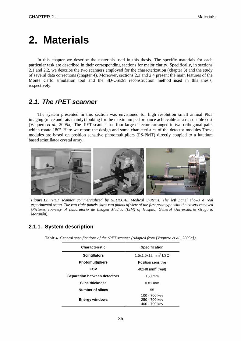
CHAPTER 2 - Materials
35
2. Materials
In this chapter we describe the materials used in this thesis. The specific materials for each
particular task are described in their corresponding sections for major clarity. Specifically, in sections
2.1 and 2.2, we describe the two scanners employed for the characterization (chapter 3) and the study
of several data corrections (chapter 4). Moreover, sections 2.3 and 2.4 present the main features of the
Monte Carlo simulation tool and the 3D-OSEM reconstruction method used in this thesis,
respectively.
2.1. The rPET scanner
The system presented in this section was envisioned for high resolution small animal PET
imaging (mice and rats mainly) looking for the maximum performance achievable at a reasonable cost
[Vaquero et al., 2005a]. The rPET scanner has four large detectors arranged in two orthogonal pairs
which rotate 180º. Here we report the design and some characteristics of the detector modules.These
modules are based on position sensitive photomultipliers (PS-PMT) directly coupled to a lutetium
based scintillator crystal array.
Figure 12. rPET scanner commercialized by SEDECAL Medical Systems. The left panel shows a real
experimental setup. The two right panels show two points of view of the first prototype with the covers removed
(Pictures courtesy of Laboratorio de Imagen Médica (LIM) of Hospital General Universitario Gregorio
Marañón).
2.1.1. System description
Table 4. General specifications of the rPET scanner (Adapted from [Vaquero et al., 2005a]).
Characteristic Specification
Scintillators 1.5x1.5x12 mm3 LSO
Photomultipliers Position sensitive
FOV 48x48 mm2 (real)
Separation between detectors 160 mm
Slice thickness 0.81 mm
Number of slices 55
Energy windows 100 - 700 kev 250 - 700 kev 400 - 700 kev

CHAPTER 2 - Materials
36
rPET detectors are based on 1.5×1.5×12 mm3 MLS crystals (Glendfield Partners, Canada) with
all the facets mechanically polished (Figure 13A). MLS is a not-hygroscopic and rugged material
based on lutetium, what makes it radioactive, producing a background of around 260 cps per cubic
centimeter [Miyaoka et al., 2001, Melcher and Schweitzer, 1992]. The individual crystals are
assembled on a 30×30 matrix with 100 microns thick Lumirror reflector (Toray Corp., Japan) between
crystals, achieving a packing fraction of 88%. The array is optically coupled to an H8500 flat-panel
PS-PMT (Hamamatsu, Japan) [Engels et al., 2003, Inadama et al., 2004] using silicon grease BC-630
(Bicron/SaintGobain, The Netherlands) which index of refraction is 1.465. Weighted position readout
circuits preprocess the 64 signals from the 8×8 anodes matrix which, in turn, are amplified without
shaping and digitized using a charge integrating converter (A&D Precision, MA). This readout
scheme, although in its current implementation suffers from the same detector dead-time limitation
described in [Riboldi et al., 2003], implements a modified center of gravity (COG) calculation for the
event positioning [Pani et al., 2003, Olcott et al., 2003, Majewski et al., 2001, Popov et al., 2003,
Siegel et al., 1996, Lage et al., 2010], and integrates gain compensation for each individual anode.
The amplification electronics, including the trigger signal for coincidence detection and the high
voltage supply are contained in three stacked PCBs (Printed Circuit Boards), forming a base attached
to the back of the PS-PMT (Figure 13B). The whole assembly is enclosed in a light tight, lead-
shielded aluminum box that doubles as an EM screen. Previous works referenced in the literature
[Miyaoka et al., 2001, Vaquero et al., 1998, Majewski et al., 2001] have demonstrated that this
combination of PS-PMTs, high light output scintillators arrays and charge sensitive readouts schemes
is well suited for high resolution, high sensitivity PET imaging systems.
(A) (B)
Figure 13. (A): MLS crystals matrix. (B): rPET detector module. The crystal array and the PS-PMT are
packed together in a black Delrim enclosure, with the detector electronics directly coupled to the PS-PMT
sockets (front). This assembly fits on the aluminum Pb-shielded box (back-right) in which the detector is
locked. The RF shield (back-left) closes the detector box. (Pictures courtesy of LIM of Hospital General
Universitario Gregorio Marañón).
2.1.2. Data acquisition and processing
Figure 14 shows a flowchart of the data processing in rPET scanner. The analog base output is
directly connected to the charge integrating ADCs (Analog-to-digital converters) with a multi-coaxial
cable, and the digitized events are screened and histogramed. A modified COG algorithm eliminates
from the position calculation those anode signals with poor signal-to-noise ratio. The method used to
filter these signals is based on a dynamic threshold value, calculated for each event. If the integrated
charge for any given signal is greater than the calculated threshold, it is included in the COG
calculation; otherwise the anode signal is excluded. The resulting position value is mapped to an
individual crystal by means of a look-up table (LUT) previously computed, and the energy value for
that event is histogramed on the corresponding crystal spectrum.

CHAPTER 2 - Materials
37
Figure 14. Flowchart of the data processing in rPET scanner (Adapted from [Vaquero et al., 2005a]).
The data acquisition trigger is done using the signal from the last dynode of the PS-PMT,
amplified at the base and filtered by a high/low discriminator that selects those events whose energy is
within the hardware energy window (50-800 keV). This single, wide energy window is set for the
whole PS-PMT, preventing the truncation of individual crystal spectra with different gains. This
scheme allows compensating for gain variation across the detector FOV by means of a variable
software energy window whose variation follows the gain variation pattern.
The rPET system acquires data in 3D-mode only, and images are reconstructed by either single
slice rebinning (SSRB) followed by 2D filtered backprojection or 2D-OSEM, or by 3D-OSEM.

CHAPTER 2 - Materials
38
2.2. The Argus PET/CT scanner
The Sedecal Argus, formerly marketed by GE Healthercare as the GE eXplore Vista [Wang et al.,
2006b], is based on the design of the National Institutes of Health ATLAS preclinical PET system
[Seidel et al., 2003].
Figure 15. Argus scanner commercialized by SEDECAL Medical Systems. (Picture courtesy of SEDECAL4).
2.2.1. System description
The system, described in Table 5, consists of 36 detector modules arranged in two rings around a
circle such that the face-to-face diameter of each ring is 11.8 cm. Each detector module is placed in
time coincidence with the 14 opposite modules to give an effective transverse field of view of 6.7 cm
and an axial FOV of 4.8 cm. Each detector module consists of a 13×13 array of 1.45×1.45 mm2 by 15
mm long elements optically isolated from each other by reflective material. A notable feature is its
depth of interaction (DOI) or parallax-correcting capability, implemented by dual-scintillator phosphor
sandwich (phoswich) detector modules [Carrier et al., 1988, Dahlbom et al., 1997, Seidel et al., 1999,
Dahlbom et al., 1998]. These modules comprise densely packed, square arrays of small-crosssection
phoswich elements, each element created by optically joining together end to end two different
scintillators. In Argus, this crystal pair is cerium-doped lutetium–yttrium orthosilicate (LYSO) in the
front crystal layer and cerium-doped gadolinium orthosilicate (GSO) in the rear layer. The GSO layer
is optically coupled to a Hamamatsu R8520-C12 PSPMT to create the Argus detector module.
These phoswich elements play the role of the usual single scintillation crystal in other types of
small-animal PET scanners. Scintillation light from a phoswich element, each optically isolated from
its neighbors, decays with the characteristic light decay time (LYSO, 40 ns; GSO, 60 ns) of the
scintillator in which the annihilation -ray from the target interacted. Thus, if the light decay time of
the event can be determined for every event, then the interaction site can be assigned to one or the
other phoswich scintillator, front or back. This knowledge, in turn, locates the interaction site to the
center of either scintillator and provides a two-valued estimate of the (radial) DOI of the event.
Knowledge of this depth, in turn, allows for partial compensation of the DOI effect (or parallax error)
that progressively degrades radial spatial resolution with increasing radial position in all PET scanners
with cylindrical geometry. Thus, a DOI correcting system can use crystal elements of greater
(combined) depth to improve sensitivity while at the same time suppressing resolution and resolution
uniformity degradation with increasing radial position—effects that otherwise occur in machines with
4 http://www.sedecal.com

CHAPTER 2 - Materials
39
identical geometry but without this capability.
Table 5. Sedecal Argus PET System description [Wang et al., 2006b]
The Argus PET/CT model integrates, besides the PET modality, a fully functional CT system.
The CT is composed of a micro-focus X-ray tube and a digital flat panel detector (flat panel CMOS
technology with a micro-columnar CsI:Tl scintillator plate) on a rotary gantry. Table 6 reports the
main characteristics of the Argus CT system.
Table 6. Sedecal Argus CT System description. (Adapted from [Vaquero et al., 2008])
Item Characteristic Specification
FOV 75 75 mm
Detector Detector Active Area 120 120 mm
Pixel Size 50, 100, 200 μm
Scintillation Material Csl:Tl
X-Ray Source Focal Spot 35 μm
X-Ray Peak energy 0-50 kV (Variable)
Max Current 1 mA
Max Power 50 Watts continuous
2.2.2. Data acquisition
ARGUS PET system acquires coincidence events in 3D using a data acquisition system based on
charge integrating ADC modules (A&D Precision, MA) and a custom coincidence logic controller, all
of them connected to the main signal processor using high-speed Ethernet links. The user may select
the CT only, PET only or dual scan in any order. Dataset are intrinsically registered and fusion display
tools are available in a single workstation.
Argus PET images are reconstructed either by Fourier rebinning (FORE) followed by 2D filtered
backprojection or 2D-OSEM, or by 3D-OSEM.

CHAPTER 2 - Materials
40
2.3. Monte Carlo simulations: PeneloPET
As it was discussed in chapter 1 (section 1.4), there are several Monte Carlo codes that simulate
the transport of radiation through matter, e.g. GEANT4 [Agostinelli, 2003], MCNP [Briesmeister,
1993], EGS4 [Kawrakow and Bielajew, 1998], and PENELOPE [Baró et al., 1995, Salvat et al.,
2006]. Either based upon these codes, or in tables of photon cross-sections, a number of tools for PET
simulation have been developed, such as SIMSET [Harrison et al., 1993], PETSIM [Thomson et al.,
1992] or Eidolon [Zaidi and Scheurer, 1999], based on MCNP, and GATE, based in GEANT4 [Jan et
al., 2004a]. Probably one of the most widely known is GATE which, being based in GEANT4, can
include a large variety of photon detectors and targets the large community of high energy and nuclear
physics users that have acquaintance with GEANT4 [Buvat and Lazaro, 2006]. GEANT4 is powerful
and flexible enough to simulate PET scanners; however, its learning curve is both steep and long. A
superficial knowledge of C++ is insufficient to optimally use GEANT4, and the installation process
requires more than basic computer skills. This is why GATE was developed. GATE consists of
hundreds of classes that provide useful functionalities for PET simulations. No C++ programming is
involved and thus it is easier to learn and use, unless there is a need to create new classes to address
specific problems.
However, we chose PeneloPET [España et al., 2009] as our PET simulation tool. PeneloPET is
based on PENELOPE [Baró et al., 1995], a Monte Carlo code which is written using FORTRAN.
PENELOPE is a Monte Carlo code for the simulation of the transport in matter of electrons, positrons
and photons with energies from a few hundred eV to 1 GeV. It is then less generally aimed as
GEANT4, but it suits well PET needs, it is fast and robust, and it is extensively used for other medical
physics applications, particularly for dosimetry and radiotherapy [Sempau and Andreo, 2006,
Panettieri et al., 2007, Vilches et al., 2007].
We chose PeneloPET, instead of another simulation tool, because it was developed by our group
(GFN, Universidad Complutense Madrid), which means a benefit whether modifications are required
in order to fit our needs of this work. Besides, PeneloPET is an easy to use simulation package. It
allows for realistic simulations, including high detail in physics and electronics processing of detector
pulses. The ample variety of detector configurations allowed by the combination GEANT/GATE is
appealing, but it comes at the cost of increased need for computing resources [Buvat and Lazaro,
2006]. However, thanks to the reduction of simulation time in PeneloPET, faster simulations are
achieved without loss of simulation detail. For its versatility, speed, and easy-to-analyze outputs,
PeneloPET is a tool useful for scanner design, system response calculations, development of
corrections methods, and many other applications. In this section we describe briefly some of the main
characteristics of PeneloPET. For further details see [España et al., 2009]
2.3.1. Main features of PeneloPET
The basic components of a PeneloPET simulation are detector geometry and materials definition
(including non-detecting materials, like shiedls), source definitions, non-active materials in the field of
view of the scanner, and electronic chain of detection. All these components are defined using
parameters in the input files. Different levels of output data are available for analysis, from sinogram
and LORs histogramming to fully detailed list-mode. These data can be further exploited with the
preferred programming language, including ROOT. The detailed list-mode generates a file with all the
hits, single or coincidence events, and the corresponding information about interaction coordinates,
deposited energy in the detectors, and time and type of coincidence: random, scatter, true, with pile-
up, etc [España et al., 2009].
CHAPTER 2 - Materials
41
2.3.1.1. PeneloPET structure
The source code consists of two main modules. The first one deals with the PENELOPE
simulations and the level of detail chosen for these, and takes care of the information about scanner
detectors and materials, source and decay. This module includes the routines involved in the
distribution of isotopes and emission of particles generated in the decay processes, as well as their
interactions.
The second module post-processes the decay and interaction data generated by the first module. It
takes into account, for instance, Anger logic for positioning the interaction inside the crystal array,
detector pile-up, energy resolution in the scintillator, and aspects of the electronics, such as
coincidence time window, dead-time, time resolution, and integration time. No PENELOPE routines
are generally involved in this second module. Energy windows can be applied in this second module.
Continuous or pixelated detectors can be managed by this second stage of the simulation package.
In order to run the simulations on clusters of computers, a simple and portable Python5 script is
provided with the code. The use of Python enables to run the script under Windows, Linux/Unix, and
Mac OS X. After configuring PeneloPET for the execution of the desired setup in a single-CPU, the
Python script launches the simulation on the number of CPUs desired, with different random seeds,
and takes care of the initial activity and acquisition time for each sub-process, in order to simulate the
same number of decay events as the equivalent single-CPU run. In this way, the simulation time is
reduced proportionally to the number of CPUs employed.
2.3.1.2. Description of PeneloPET input files
Four input files have to be prepared by the user in order to set up a simulation. As an example,
Table 7 shows these input files for the simulation of a point source in the previously described rPET
scanner (section 2.1, [Vaquero et al., 2005a]).
The first input file in Table 7 (main.inp) contains the general parameters of the simulation, such
as the acquisition protocol and acquisition time. It also enables simulation of secondary particles, if
desired, and controls whether positron range and non-collinearity are taken into account. This file
contains options also for scanner rotation, energy and coincidence windows, contributions to dead
time, output format, and type of study.
In the second file (scanner.inp), which contains the scanner definition, multiple rings and layers
of crystals can be specified. Although our main goal was to simulate pixelated detectors for high-
resolution small animal PET imaging, PeneloPET is also suitable for continuous scintillator blocks or
even detectors not based on scintillators (such as CZT or silicon strips) with small or no changes.
Non-radioactive materials other than the scintillator (already defined in the file scanner.inp), such
as surrounding materials and shielding, are defined in a third file (object.inp). The radioactive source
is defined separately in a fourth input file (source.inp), which contains source geometry and
information about activity and isotope. Keeping separated definitions for sources and materials
simplifies the comparison of simulations of ideal sources, without scatter or attenuation, to more
realistic sources. Details about PeneloPET input files and options can be found in the PeneloPET
manual6.
Typical materials for crystals, shielding and phantoms are predefined in PeneloPET and, if
necessary, new materials can be created in a straightforward way. The visualization tools built in
PENELOPE (gview2d, gview3d [Salvat et al., 2006]) are also available in PeneloPET to display and
test geometries. This is especially useful during scanner design stages.
5 http://www.python.org/
6 http://nuclear.fis.ucm.es/penelopet/

CHAPTER 2 - Materials
42
Although the work presented in this thesis deal with preclinical scanners, PeneloPET is also
capable of simulating clinical PET scanners. [Abushab et al., 2011]
Table 7. PeneloPET input files needed to simulate a point source in the rPET scanner [Vaquero et al., 2005a].
Full detail about these input files and options can be found in the PeneloPET manual7. In this input file, ‘F’
stands for false or disabled option, while ‘T’ stands for true or enabled option.
--- GENERAL PARAMETERS --- (main.inp)
12345 54321 !Random number generator seeds 9000 1 F !Acquisition time (sec); Number of Frames; Read Frame List File 1000 !Limit number of interactions for each particle F T T !Secondary Particles Simulation; Positron Range; Non-Collinearity 0 180 3000 40 !Initial & Final and pos (deg); Numb of Steps per cycle; time per cycle (sec) 0. !Lower Level Energy Threshold (eV) 1000000. !Upper Level Energy Threshold (eV) 5 !Coincidence Time Window (ns) 0.1 !Trigger’s Dead-Time (ns) 150 !Integration Time (ns) 1200 !Coincidence’s Dead-Time (ns) F F T !Hits LIST; Singles LIST; Coincidences LIST F !Write LOR Histogram T 117 190 4.49684 !Write Sinogram; radial bins; angular bins; maximum radio F 99 99 55 4.48 4.2 !Write Emission Image; X Y Z voxels, Transaxial & Axial FOV (cm) F !Hits checking T !Verbose F !Neglecting events if more than 2 singles in the coincidence time window
--- SCANNER PARAMETERS --- (scanner.inp)
4 !Number of Detectors per Ring 1 !Number of Detectors in Coincidence in the same Ring 1 !Number of Rings 0. !Gap Between Rings (cm) 30 !Number of transaxial crystals per detector (columns) 30 !Number of axial crystals per detector (rows) 1 !Number of crystal layers per detector 1.2 13 0.26 1 40 0.01 !LAYER: Length (cm); Mat; E Resol.; Rise & Fall Tim (ns); Tim Error (ns) 0.16 0.16 !Pitch: Distance between centres of adjacent crystals (cm) 8. !Radius: Centre FOV - Centre Front of Detector (cm)
--- BODY PARAMETERS --- (object.inp)
C 1 0. 0. 0. 0. 1.62 5.0 0. 0. !Shape Mat X Y Z R1 R2 HEIGHT (cm) PH TH (deg)
--- SOURCE PARAMETERS --- (source.inp)
P 1E6 F 1 0.5 1. 2. 0. 0. 0. 0. 0. 0. 0. 0. 180 ! Shap Act Units Isot X Y Z R1 R2 H PH TH TH1 TH2
2.3.1.3. Description of PeneloPET output files
Output files generated by PeneloPET can offer three different levels of detail. At the highest
level, all the information about each interaction is recorded for further analysis. At the intermediate
level, just the single events and the information needed for their analysis are recorded. The possibility
of pile-up and cross talk is taken here into account. At the third, and lowest, level of detail, only
coincidence events are recorded in a compact List-mode. Information about pile-up, scatter, random
and self-coincidence events, obtained from the simulation, is also summarily available.
A coincidence event is labeled as pile-up when at least one of the single events has suffered pulse
pile-up. A coincidence is considered to be a scatter coincidence when at least one of the photons that
trigger the detectors has interacted before reaching the scintillator. A coincidence is considered a
7 http://nuclear.fis.ucm.es/penelopet/

CHAPTER 2 - Materials
43
random when the two photons in the coincidence pair come from two different, uncorrelated,
annihilation processes. Self-coincidence events may arise when the same photon, after scattering in a
first detector, reaches a second detector. If the energy deposited in each detector is above the detection
threshold, it may trigger two single events and yield a self-coincidence count. The remaining
coincidences are considered as true events.
PeneloPET generates several output histograms that help to understand the results of the
simulations, as for instance sinogram projections, LOR histogram, single and coincidence maps, and
energy spectrum. In order to simplify the reconstruction of simulated data, the format of the sinograms
conforms to that expected by the STIR library8.
ROOT [Brun and Rademakers, 1997] is an object-oriented data analysis framework that provides
tools for the analysis of experimental data. PeneloPET LIST files can be converted into ROOT format.
2.3.2. PENELOPE
As it was mentioned, PENELOPE is the core of PeneloPET. PENELOPE [Salvat et al., 2006]
consists of a package of subroutines, invoked by a main program that controls the evolution of the
stories of particle counters and accumulates the magnitudes of interest for each specific application.
These subroutines are written in the FORTRAN77 programming language, and are distributed by
Nuclear Energy Agency - Organization for Economic Co-operation and Development (NEA-OECD).
The authors are Francesc Salvat and Jose M. Fernández-Varea of the Physics Department of the
Universidad de Barcelona and Josep Sempau of the Institute of Energy of the Universidad Politécnica
de Cataluña.
The simulation of electrons and positrons includes the following types of interactions:
Hard elastic collision (θ > θ c).
Hard inelastic collision (θ > θ c).
Hard Bremsstrahlung emission.
Delta interaction.
Artificially soft event (θ<θc).
Inner-Shell impact ionization.
Annihilation (only for positrons).
Auxiliary interaction (an additional mechanism that may be defined by the user, e.g., to
simulate photonuclear interactions).
The simulation of photons includes the following interactions:
Coherent scattering (Rayleigh).
Incoherent scattering (Compton).
Photoelectric absorption.
Electron-Positron pair production.
Delta interaction.
Auxiliary interaction.
For further explanation of the physics included in these interactions the reader is referred to
[Sempau et al., 2003b].
Each interaction can lead to secondary particles which can be later tracked and simulated. For
example, the positron annihilation leads to γ photons and the photoelectric effect will lead to free
8 http://stir.sourceforge.net

CHAPTER 2 - Materials
44
electrons.
The use of PENELOPE requires preparing a main program which will be responsible for calling
PENELOPE subroutines and for storing the information about the trajectories of the particles
simulated. The main program should provide PENELOPE with the information about the geometry
and materials, and also other parameters such as type of particle, energy, position and direction of
movement of the particle to be simulated. Through appropriate use of these tools, the user can create a
simulation environment to carry out the desired studies. PENELOPE is of relatively common use in
experimental nuclear physics and medical physics [Panettieri et al., 2007].
PENELOPE includes a subroutine for generating sets of random numbers, that is based in an
algorithm due to [L'ecuyer, 1988]. This algorithm yields 32-bit real numbers distributed uniformly
over an open interval between zero and one. Its period is approximately 1018
, which can be considered
as infinite for most practical purposes.

CHAPTER 2 - Materials
45
2.4. Image reconstruction: FIRST
Small animal PET scanners require high spatial resolution and good sensitivity. To reconstruct
high-resolution images in 3D-PET, iterative methods, such as OSEM, are superior to analytical
reconstruction algorithms, although their high computational cost is still a serious drawback [Johnson
et al., 1997, Herraiz et al., 2006b]. The performance of modern computers could make iterative image
reconstruction fast enough and able of dealing with the large number of probability coefficients of the
system response matrix, in high-resolution PET scanners, which is a difficult task that prevents the
algorithms from reaching peak computing performance. As it was discussed in chapter 1 (section
1.5.3), one of the key advantages of iterative reconstructions is the ability to incorporate accurate
models of the PET acquisition process through the use of the system response matrix (SRM).
However, SRM for 3D systems are of the order of several billions of elements, which imposes serious
demands for statistical iterative methods in terms of the time required to complete the reconstruction
procedure and the computer memory needed for the storage of the SRM.
In this section we describe the FIRST algorithm, the 3D-OSEM reconstruction method used in
this thesis. Section 2.4.1 presents the main features of the standard FIRST algorithm and section 2.4.2
depicts an adaptation of FIRST algorithm, GFIRST, which uses the computing capabilities of Graphic
Processing Units (GPUs).
2.4.1. Main features of the FIRST algorithm
FIRST (Fast Iterative Reconstruction Software for (PET) tomography) is a fully 3D-OSEM non-
sinogram-based reconstruction algorithm implemented by our group (GFN, Universidad Complutense
Madrid) [Herraiz et al., 2006b], which uses a compressed SRM that contains the resolution recovery
properties of EM. This reconstruction method includes the possibility of MAP by means of a
generalized one-step late MAP-OSEM algorithm, similar to the one described in Lewitt and Matej
[2003] and Kadrmas [2004]:
, 1 ,
,
, 1 ,
ni SubsetSi in s n s
i SubsetS
y iA i j
R Sx j x j
A i j Penalty j n
(33)
where the x(j) is the activity of voxel j (j = 1, maximum voxel number V), xn,s
(j) is the expected value
of voxel j at iteration n and subiteration s, A(i, j) is the SRM, y(i) is the projection from the object
measured at LOR i (experimental data), Si is the object scatter + random coincidences at LOR i,
Penalty(j,n) is the penalty value at voxel j and iteration n, Rin is the projection estimated for the image
reconstructed at iteration n:
1
,Voxels
n n
i
j
R A i j x j
(34)
This MAP-OSEM algorithm can be considered as a generalization of the ML–EM. It incorporates
a penalty MAP function which can be chosen in different ways [Stayman and Fessler, 2001, Yu and
Fessler, 2002, Nuyts and Fessler, 2003], and scatter and random counts estimates, that may require
additional modeling of these processes. OSEM reconstruction without MAP regularization is obtained
by setting the penalty function to zero.

CHAPTER 2 - Materials
46
As it was introduced before, an important problem of iterative methods is the size of the SRM. If
the SRM does not fit in RAM, the performance of the reconstruction is affected significantly, due to
the large time required to access the hard disk. For example, for the Argus scanner described in section
2.2 [Wang et al., 2006b], for a nominal image resolution of 175 × 175 × 62 voxels (near 1.9 millions
of voxels), the number of elements in the SRM (number of LORs × number of voxels) is of the order
of 5 × 10¹³
. Storing all the elements of the SRM would require more than 10 TB. This exceeds the
resources of any ordinary workstation, making it necessary to disregard all redundant elements and to
perform approximations in order to be able to store the SRM in the limited amount of RAM of
ordinary workstations. To achieve this goal, three techniques were used in the FIRST algorithm:
null or almost-null element removal (matrix sparseness),
intensive use of system symmetries,
compression of the resulting SRM employing quasi-symmetries.
Using these techniques, it was possible to reduce the memory needed to store the SRM well
below 150 MB, being the reconstructed images indistinguishable from the ones obtained without
compression. This fact allows keeping the whole response matrix of the system inside the RAM
present in ordinary industry-standard computers, so that the reconstruction algorithm can achieve near
peak performance. Besides, the elements of the SRM are stored as cubic spline profiles and matched to
voxel size during reconstruction. In this way, the advantages of on-the-fly calculation and of fully
stored SRM are combined. The on-the-fly part of the calculation (matching the profile functions to
voxel size) of the SRM accounts for 10–30% of the reconstruction time, depending on the number of
voxels chosen.
In addition, the FIRST algorithm can include the usage of the message passing interface (MPI)
protocol [Gropp et al., 1999] to launch parallel tasks on the available CPUs (or CPU cores) in a cluster
of computers.
The flexibility, reduced reconstruction time, accuracy and resolution of the resulting images
prove that the methodologies used to implement the FIRST reconstruction can be applied to real
studies of high-resolution small animal PET scanners.
2.4.2. GFIRST: GPU-Based Fast Iterative Reconstruction of Fully 3-D PET Sinograms
Graphics Processing Units (GPU) has been proposed for many years as potential accelerators in
complex scientific problems [General-Purpose Computing on Graphics Processing Units repository]
like image reconstruction, with large amount of data and high arithmetic intensity. Indeed,
tomographic reconstruction codes are suitable for massive parallelization, as the two main time-
consuming parts of the code (forward and backward projection) can be organized as single instruction
multiple data (SIMD) tasks and distributed among the available processing units by assigning part of
the data to each unit [Jones and Yao, 2004, Hong et al., 2007].
GFIRST is an adaptation of FIRST to use the efficient computing capabilities of GPUs developed
by our group [Herraiz et al., 2011]. The main goal was to obtain a significant acceleration of the
algorithm without compromising the quality of the reconstructed images, and with speed-ups large
enough to compete with the reconstruction times obtained in a cluster of CPUs. The code does not
have GPU-specific optimizations, allowing possible future modifications with no significant additional
effort. Besides, the GPU code is as similar as possible to the CPU code, what makes it easier to handle
and debug. Indeed, approximations in the forward and backward projection kernels were avoided and
the same SRM as in the original CPU code was used in order to avoid a loss of accuracy or artifacts in
the final images.

CHAPTER 2 - Materials
47
At variance with previously proposed reconstruction codes for the GPU [Pratx et al., 2009,
Reader et al., 2002] which dealt with list-mode data, GFIRST was designed to work with sinograms
[Fahey, 2002]. Although list-mode data, for which all the relevant information from each detected
coincidence is stored, might provide optimal images, sinogram data organization also has some
interesting features. First, sinograms are commonly used in most of the current commercial scanners
[Fahey, 2002], and they are often easily available to the user. Usually, their size is smaller than list-
mode files, so they are easier to handle and store. Furthermore, in a sinogram, data are spatially
ordered and can thus be accessed in a simple and ordered way. This allows for very fast backward
projection implementations. Finally, under certain approximations imposed by the sinogram, the
simulated system exhibits many symmetries, thus reducing the size of the SRM.
The code is implemented in CUDA [NVIDIA CUDA Programming Guide v.2.5.0], an application
programming interface (API), which allows writing programs in C language with extensions to
execute part of them (CUDA kernels) on the GPU. Since forward and backward projections take up
most of the reconstruction time, only these two steps are implemented as CUDA kernels called from
the main reconstruction C code, running in the CPU. Figure 16 shows the data flow between CPU and
GPU.
Figure 16. Flowchart of the implementation of the code in the GPU [Herraiz et al., 2011].
Due to the large number of threads that can be executed in parallel on GPUs, the usual
bottlenecks of these implementations are memory access. GFIRST uses texture memory, a kind of
global memory available in the GPU that is allocated and indexed for fast access [Sanders and
Kandrot, 2010 ].
As shown in Figure 16, three 3-D textures are defined in GFIRST: one for the image being
reconstructed, another for the SRM, and a third corresponding to the corrections obtained after
comparing measured and estimated data. The SRM is uploaded into GPU global memory as a 3-D
array and then attached to a 3-D texture at the start of the program.
With GFIRST we achieved a very significant improvement in reconstruction time (with a speed-
up factor of up to 72, see Table 8) for the fastest GPU compared to a single core of a high-end CPU.
This is remarkable, as FIRST had already been shown to be a highly optimized reconstruction code.

CHAPTER 2 - Materials
48
Table 8. Reconstruction time for one image (one bed, one-frame acquisition, one full iteration) for different
architectures [Herraiz et al., 2011].
For further information about the GFIRST implementation the reader is referred to [Herraiz et al.,
2011].
In this thesis (see chapter 5, section 5.2) we use an adaptation of GFIRST, which instead of using
the SRM, uses the PSF information with a new regularization method [Vicente et al., 2012b].
CHAPTER 2 - Materials
49
2.5. References Agostinelli, S. 2003. GEANT4 - a simulation toolkit. Nucl. Inst. Meth. In Phy. Res. A, 506, 250-303.
Baró, J., Sempau, J., Fernández-Varea, J. M. & Salvat, F. 1995. PENELOPE: An algorithm for Monte Carlo simulation of the
penetration and energy loss of electrons and positrons in matter. Nucl. Inst. Meth. In Phy. Res. B, 100, 31-46.
Briesmeister, J. F. 1993. MNCP 4 A, Monte Carlo N-Particle Transport System. Los Alamos, New Mexico: Los Alamos
National Laboratory.
Brun, R. & Rademakers, F. 1997. ROOT - An object oriented data analysis framework. Nucl. Inst. & Meth. in Phys. Res. A,
389, 81-86.
Buvat, I. & Lazaro, D. 2006. Monte Carlo simulations in emission tomography and GATE: An overview. Nucl. Inst. Meth. In
Phy. Res. A, 569, 323-29.
Carrier, C., Martel, C., Schmitt, D. & Lecomte, R. 1988. Design of a high resolution positron emission tomograph using solid
state scintillation detectors. Nuclear Science, IEEE Transactions on, 35, 685-690.
Dahlbom, M., MacDonald, L. R., Eriksson, L., Paulus, M., Andreaco, M., Casey, M. E. & Moyers, C. 1997. Performance of a
YSO/LSO phoswich detector for use in a PET/SPECT system. Nuclear Science, IEEE Transactions on, 44, 1114-
1119.
Dahlbom, M., MacDonald, L. R., Schmand, M., Eriksson, L., Andreaco, M. & Williams, C. 1998. A YSO/LSO phoswich
array detector for single and coincidence photon imaging. Nuclear Science, IEEE Transactions on, 45, 1128-1132.
Desco, M. Cursos 97-98, 98-99, 00-01. Asignatura "Bioestadística" (Especialidad de Laboratorio). Escuela Técnico
Profesional de la Salud de la Comunidad de Madrid. Hospital General Universitario Gregorio Marañón.
Engels, R., Clemens, U., Kemmerling, G. & Schelten, J. 2003. High spatial resolution scintillation detector based on the
H8500 photomultiplier. In: Nuclear Science Symposium Conference Record, 2003 IEEE, 19-25 Oct. 2003 2003.
692-695 Vol.1.
España, S., Herraiz, J. L., Vicente, E., Vaquero, J. J., Desco, M. & Udias, J. M. 2009. PeneloPET, a Monte Carlo PET
simulation tool based on PENELOPE: features and validation. Phys Med Biol, 54, 1723-42.
Fahey, F. H. 2002. Data acquisition in PET imaging. J Nucl Med Technol, 30, 39-49.
General-Purpose Computing on Graphics Processing Units repository [Online]. Available: www.gpgpu.org. [September
2010].
Gropp, W., Lusk, E. & Skjellum, A. 1999. Using MPI: portable parallel programming with the message-passing interface,
MIT Press.
Harrison, R. L., Vannoy, S. D., Haynor, D. R., Gillispie, S. B., Kaplan, M. S. & Lewellen, T. K. 1993. Preliminary
Experience With The Photon History Generator Module Of A Public-domain Simulation System For Emission
Tomography. In: Nuclear Science Symposium and Medical Imaging Conference, 1993., 1993 IEEE Conference
Record., 31 Oct-6 Nov 1993 1993. 1154-1158.
Herraiz, J. L., España, S., Cabido, R., Montemayor, A. S., Desco, M., Vaquero, J. J. & Udias, J. M. 2011. GPU-Based Fast
Iterative Reconstruction of Fully 3-D PET Sinograms. Nuclear Science, IEEE Transactions on, 58, 2257-2263.
Herraiz, J. L., España, S., Vaquero, J. J., Desco, M. & Udias, J. M. 2006b. FIRST: Fast Iterative Reconstruction Software for
(PET) tomography. Phys. Med. Biol., 51, 4547-4565.
Hong, I. K., Chung, S. T., Kim, H. K., Kim, Y. B., Son, Y. D. & Cho, Z. H. 2007. Ultra Fast Symmetry and SIMD-Based
Projection-Backprojection (SSP) Algorithm for 3-D PET Image Reconstruction. Medical Imaging, IEEE
Transactions on, 26, 789-803.
Inadama, N., Murayama, H., Watanabe, M., Omura, T., Yamashita, T., Kawai, H., Umehara, T., Kasahara, T., Orita, N. &
Tsuda, T. 2004. Performance of a PET detector with a 256ch flat panel PS-PMT. Nuclear Science, IEEE
Transactions on, 51, 58-62.
Jan, S., Santin, G., Strul, D., Staelens, S., Assié, K., Autret, D. & Avner, S. 2004a. GATE: a simulation toolkit for PET and
SPECT. Phys. Med. Biol., 49, 4543-4561.
Johnson, C. A., Seidel, J., Carson, R. E., Gandler, W. R., Sofer, A., Green, M. V. & Daube-Witherspoon, M. E. 1997.
Evaluation of 3D reconstruction algorithms for a small animal PET camera. IEEE Trans. Nuc. Sci., 44, 1303-1308.
Jones, M. D. & Yao, R. 2004. Parallel programming for OSEM reconstruction with MPI, OpenMP, and hybrid MPI-
OpenMP. In: Nuclear Science Symposium Conference Record, 2004 IEEE, 16-22 Oct. 2004 2004. 3036-3042.
Kadrmas, D. J. 2004. LOR-OSEM: statistical PET reconstruction from raw line-of-response histograms. Phys. Med. Biol., 49,
4731-4744.
Kawrakow, I. & Bielajew, A. F. 1998. On the condensed history technique for electron transport. Nucl. Inst. Meth. In Phy.
Res. B, 142, 253-280.
L'Ecuyer, P. 1988. Efficient and portable combined random number generators. In: ACM, 1988 New York. ACM, 742-51.
Lage, E., Tapias, G., Villena, J., Desco, M. & Vaquero, J. J. 2010. Data acquisition electronics for gamma ray emission
tomography using width-modulated leading-edge discriminators. Physics in Medicine and Biology, 55, 4291.
Lewitt, R. M. & Matej, S. 2003. Overview of methods for image reconstruction from projections in emission computed
tomography. In: IEEE NSS-MIC, 2003. 1588-1611.
Majewski, S., Kieper, D., Curran, E., Keppel, C., Kross, B., Palumbo, A., Popov, V., Wisenberger, A. G., Welch, B., Wojcik,
R., Williams, M. B., Goode, A. R., More, M. & Zhang, G. 2001. Optimization of dedicated scintimammography
procedure using detector prototypes and compressible phantoms. Nuclear Science, IEEE Transactions on, 48, 822-
829.
Melcher, C. L. & Schweitzer, J. S. 1992. Cerium-doped lutetium oxyorthosilicate: a fast, efficient new scintillator. Nuclear
Science, IEEE Transactions on, 39, 502-505.
CHAPTER 2 - Materials
50
Miyaoka, R. S., Kohlmyer, S. G., Jinhun, J. & Lewellen, T. K. 2001. Performance characteristics of a second generation
micro crystal element (MiCE2) detector. In: Nuclear Science Symposium Conference Record, 2001 IEEE, 4-10
Nov. 2001 2001. 1124-1127 vol.2.
Nuyts, J. & Fessler, J. A. 2003. A penalized-likelihood image reconstruction method for emission tomography compared to
postsmoothed maximum-likelihood with matched spatial resolution. IEEE Trans Med Imaging, 1042-1052.
NVIDIA CUDA Programming Guide v.2.5.0 [Online]. Available:
http://developer.nvidia.com/object/gpu_programming_guide.html. [September 2010].
Olcott, P. D., Talcott, J. A., Levin, C. S., Habte, F. & Foudray, A. M. K. 2003. Compact readout electronics for position
sensitive photomultiplier tubes. In: Nuclear Science Symposium Conference Record, 2003 IEEE, 19-25 Oct. 2003
2003. 1962-1966 Vol.3.
Panettieri, V., Wennberg, B., Gagliardi, G., Duch, M. A., Ginjaume, M. & Lax, I. 2007. SBRT of lung tumours: Monte Carlo
simulation with PENELOPE of dose distributions including respiratory motion and comparison with different
treatment planning systems. Phys Med Biol, 52, 4265-81.
Pani, R., Pellegrini, R., Cinti, M. N., Trotta, C., Trotta, G., Garibaldi, F., Scafè, R. & Del Guerra, A. 2003. Flat Panel PMT
for photon emission imaging. Nuclear Instruments and Methods in Physics Research Section A: Accelerators,
Spectrometers, Detectors and Associated Equipment, 505, 590-594.
Popov, V., Majewski, S. & Weisenberger, A. G. 2003. Readout electronics for multianode photomultiplier tubes with pad
matrix anode layout. In: Nuclear Science Symposium Conference Record, 2003 IEEE, 19-25 Oct. 2003 2003.
2156-2159 Vol.3.
Pratx, G., Chinn, G., Olcott, P. D. & Levin, C. S. 2009. Fast, Accurate and Shift-Varying Line Projections for Iterative
Reconstruction Using the GPU. Medical Imaging, IEEE Transactions on, 28, 435-445.
Reader, A. J., Ally, S., Bakatselos, F., Manavaki, R., Walledge, R. J., Jeavons, A. P., Julyan, P. J., Sha, Z., Hastings, D. L. &
Zweit, J. 2002. One-pass list-mode EM algorithm for high-resolution 3-D PET image reconstruction into large
arrays. Nuclear Science, IEEE Transactions on, 49, 693-699.
Riboldi, S., Seidel, J., Green, M., Monaldo, J., Kakareka, J. & Pohida, T. 2003. Investigation of signal readout methods for
the Hamamatsu R8500 flat panel PSPMT. In: Nuclear Science Symposium Conference Record, 2003 IEEE, 19-25
Oct. 2003 2003. 2452-2456 Vol.4.
Salvat, F., Fernández-Varea, J. M. & Sempau, J. 2006. PENELOPE-2006: A Code System for Monte Carlo Simulation of
Electron and Photon Transport, France, NEA.
Sanders, J. & Kandrot, E. 2010 CUDA by Example: An Introduction to General-Purpose GPU Programming, Addison-
Wesley.
Seidel, J., Vaquero, J. J. & Green, M. V. 2003. Resolution uniformity and sensitivity of the NIH ATLAS small animal PET
scanner: Comparison to simulated LSO scanners without depth-of-interaction capability. Nuclear Science, IEEE
Transactions on, 50, 1347-1350.
Seidel, J., Vaquero, J. J., Siegel, S., Gandler, W. R. & Green, M. V. 1999. Depth identification accuracy of a three layer
phoswich PET detector module. Nuclear Science, IEEE Transactions on, 46, 485-490.
Sempau, J. & Andreo, P. 2006. Configuration of the electron transport algorithm of PENELOPE to simulate ion chambers.
Phys Med Biol, 51, 3533-48.
Sempau, J., Fernández-Varea, J. M., Acosta, E. & Salvat, F. 2003b. Experimental benchmarks of the Monte Carlo code
PENELOPE. Nucl. Inst. Meth. In Phy. Res. B, 207, 107-123.
Siegel, S., Silverman, R. W., Yiping, S. & Cherry, S. R. 1996. Simple charge division readouts for imaging scintillator arrays
using a multi-channel PMT. Nuclear Science, IEEE Transactions on, 43, 1634-1641.
Stayman, W. & Fessler, J. A. 2001. Nonnegative Definite Quadratic Penalty Design for Penalized-Likelihood Reconstruction.
In: IEEE Nuc. Sci. Symp., 2001.
Thomson, C. J., Moreno-Cantu, J. & Picard, Y. 1992. PETSIM: Monte Carlo simulation of all sensitivity and resolution
parameters of cylindrical positron imaging systems. Phys. Med. Biol., 37, 731-749.
Vaquero, J. J., Lage, E., Ricon, L., Abella, M., Vicente, E. & Desco, M. 2005a. rPET detectors design and data processing.
In: Nuclear Science Symposium Conference Record, 2005 IEEE, 23-29 Oct. 2005 2005a. 2885-2889.
Vaquero, J. J., Redondo, S., Lage, E., Abella, M., Sisniega, A., Tapias, G., Montenegro, M. L. S. & Desco, M. 2008.
Assessment of a New High-Performance Small-Animal X-Ray Tomograph. Nuclear Science, IEEE Transactions
on, 55, 898-905.
Vaquero, J. J., Seidel, J., Siegel, S., Gandler, W. R. & Green, M. V. 1998. Performance characteristics of a compact position-
sensitive LSO detector module. Medical Imaging, IEEE Transactions on, 17, 967-978.
Vicente, E., Herraiz, J. L., Seidel, J., Green, M. V., Desco, M., Vaquero, J. J. & Udias, J. M. 2012b. Regularization of 3D
Iterative Reconstruction for a Limited-Angle PET Tomograph. In: Nuclear Science Symposium Conference
Record (NSS/MIC), 2012 IEEE (Accepted), 2012b.
Vilches, M., García-Pareja, S., Guerrero, R., Anguiano, M. & Lallena, A. M. 2007. Monte Carlo simulation of the electron
transport through thin slabs: A comparative study of PENELOPE, GEANT3, GEANT4, EGSnrc and MCNPX.
Nucl. Inst. Meth. In Phy. Res. B, 254, 219-30.
Wang, Y., Seidel, J., Tsui, B. M., Vaquero, J. J. & Pomper, M. G. 2006b. Performance evaluation of the GE healthcare
eXplore VISTA dual-ring small-animal PET scanner. J Nucl Med, 47, 1891-900.
Yu, D. F. & Fessler, J. A. 2002. Edge-preserving tomographic reconstruction with nonlocal regularization image processing.
IEEE Trans Med Imaging, 21, 159-173.
Zaidi, H. & Scheurer, C. 1999. An object-oriented Monte Carlo simulator for 3D cylindrical positron tomographs. Comput.
Methods Programs Biomed., 58, 133-45.

CHAPTER 3- Performance Evaluation of Preclinical PET Scanners
51
3. Performance Evaluation of Preclinical PET Scanners
Due to the nature of the underlying physical phenomena, design and engineering of PET systems
involve a compromise of sensitivity and spatial resolution specifications which are difficult to
optimize simultaneously. For this reason, it can be found in the literature multiple architectures and
designs aiming to different performance balance depending on the final application of the system
[Weber and Bauer, 2004, Vaquero and Desco, 2005]. In order to compare systems it is necessary to
characterize the performance of the scanners in terms of objective parameters.
The evaluation of a PET tomograph consists of quantitative measurements with a standardized
methodology, which sets a baseline of system performance under typical imaging conditions. The
measurement procedure should be as independent as possible of the PET scanner under test and
applicable to a wide range of models and geometries. Standardization facilitates acceptance testing,
routine performance monitoring and comparison among systems from different vendors or different
designs from a given vendor [Goertzen et al., 2012]. To address this need for a standard set of
measurements the NEMA NU 4 standard was published in 2008 [NEMA-NU4, 2008]. Prior to this,
there was no agreed upon method to evaluate the performance of preclinical PET systems and as a
result manufacturers could not provide specifications for these PET systems in the same way in which
specifications for clinical systems could be provided under the NEMA NU 2-1994 [NEMA-NU2,
1994] and NU 2-2001 [NEMA-NU2, 2001] standards. An additional consequence of the previous lack
of a NEMA standard for preclinical PET systems is that performance evaluation papers of earlier
preclinical PET systems used ad-hoc modifications from the NEMA standard specified for clinical
PET systems making it difficult to compare these early systems both to each other and to newer
scanners.
The standard protocols to measure performance include two types of tests, some designed to
study the intrinsic parameters of the scanner such as spatial resolution or sensitivity, and others aiming
to estimate the accuracy of the corrections involved in the reconstruction of images. These tests
estimate the following standardized performance parameters:
Sensitibity
Spatial resolution
Energy resolution
Scatter Fraction
Noise equivalent count (NEC) rate
Image quality from a standard phantom
Comparison of scanners based upon standardized procedures, and analysis of the ability of these
procedures to measure the performance of the scanner is of paramount importance in PET design
research. In this chapter we survey the contributions in this area made by this thesis. In section 3.1 of
this chapter we present an application of the standard evaluation protocols to the characterization of
the rPET [Vaquero et al., 2005b] and the Argus [Wang et al., 2006b] scanners. Further, section 3.2
shows a study of the evaluation protocol itself, by assessing the accuracy of the NEMA NU 4-2008
procedure to estimate the scatter fraction from 18
F acquisitions and also the problems it faces when a
radionuclide with a lager positron range as 68
Ga is used.

CHAPTER 3- Performance Evaluation of Preclinical PET Scanners
52
3.1. Characterization of rPET & Argus scanners
As it was mentioned above, in this section we present the performance evaluation of rPET and
Argus preclinical PET scanners [Vicente et al., 2006 , Goertzen et al., 2012]. Since part of this work
was done prior to the publication of the final version of the NEMA NU 4-2008 standard, some of the
tests were performed in slightly different ways for each scanner. This was taken into account during
the interpretation of the results of both scanners.
3.1.1. Materials & Methods
3.1.1.1. Sensitivity
The sensitivity of a PET scanner represents its ability of detecting coincident photons emitted
from inside the FOV of the scanner. It is mainly determined by two parameters of the scanner:
geometry and detection efficiency for 511 keV photons. The scanner geometry defines the fraction of
the total solid angle covered. Small-diameter and large axial FOV geometries typically lead to high-
sensitivity scanners. Given the geometry, the efficiency of a PET detector depends on the type of
detector being used. Usually, high density and atomic number scintillation detectors provide high
stopping power for PET imaging with acceptable energy resolution. A high stopping power, which
allows for shorter crystals, is also desirable for the reduction of parallax error due to depth of
interaction [Bailey, 2005].
Acquisition method
The NU 4-2008 protocol for measuring sensitivity (section 5 of [NEMA-NU4, 2008]) uses a 22
Na
point source. However, in previous versions of the draft, a line source was proposed and this was the
method used for both scanners. Table 9 shows the acquisitions done with each scanner.
Table 9. Acquisitions employed to measure the sensitivity of rPET and Argus scanners
rPET scanner Argus scanner
Phantom
Line source (capillary)
Inner diameter 1.0 mm Length = 7.3 cm
Line source (capillary)
Inner diameter 1.0 mm Length = 6 cm
Isotope 18
F 18
F
Activity (Ci) 7 27 25 23
Energy Windows (keV) 100 - 700 100 - 700 250 - 700 400 - 700
Comments
The line source is placed at the center of the FOV aligned along the geometric axis of the scanner.
The line source is wrapped in 10 layers of Al foil and placed at the center of the FOV aligned along the geometric axis of the scanner.

CHAPTER 3- Performance Evaluation of Preclinical PET Scanners
53
Data processing and analysis
The absolute central point sensitivity (ACS) was computed from the following expression:
100
·
2(%)
BRAL
FOV
CACS
axial
(35)
where: C: Measured count rate (cps)
L: Capillary length filled with 18
F solution
A: Activity of the source (Bq)
BR: Branching ratio of the source (BR(18
F) = 0.97)
FOVaxial: FOV length in axial direction.
The factor 2 is needed to estimate the ACS from a line source measurement as it is explained in
[Cherry et al., 2003]. This assumes simple scanner geometries but it has been tested with simulations
that the factor of 2 is accurate enough for both scanners presented here.
3.1.1.2. Spatial resolution
Spatial resolution can be defined as the minimum distance at which two point sources can be
acquired and disentangled by the scanner [Bailey, 2005]. Spatial resolution is usually measured from
the width of the profile obtained when an object much smaller than the expected resolution of the
system is imaged. A common method consists of imaging a point source and measuring the point
spread function (PSF). This measurement corresponds to the best resolution of the system under ideal
conditions. Usually, the resolution is expressed as the full width at half maximum (FWHM) of the
profile. Very often this profile is approximated by a Gaussian function [Bailey, 2005].
There are many factors that influence resolution:
Non-zero positron range after radionuclide decay.
Non-collinearity of the annihilation photons due to the residual momentum of the
positron.
Distance between detectors.
Width of detectors.
Stopping power of the scintillator.
Incident angle of the photon at the detector.
Depth of the interaction of the photon.
Number of angular samples.
Reconstruction parameters (matrix size, reconstruction filter, ...).
Usually, the resolution is measured along several directions across the FOV of the PET scanner
such as transaxial and axial, as sampling is not necessarily equal in all directions. Generally, ring-PET
systems are over-sampled transaxially (in the x-y plane), while axial (z-direction) sampling is just
enough to realize the intrinsic resolution of the detectors. Transaxial resolution is often measured for
both radial and tangential directions at different distances off the central axis of the scanner, as it
changes in ring geometries at different locations in the x-y plane [Bailey, 2005].

CHAPTER 3- Performance Evaluation of Preclinical PET Scanners
54
Acquisition method
The section 3 of NU 4-2008 protocol [NEMA-NU4, 2008] proposes to use a 22
Na point source to
measure the spatial resolution. This was the procedure employed in rPET scanner; however, since the
Argus spatial resolution was measured before the publication of the final version of this protocol, for
this scanner the measurement was performed using a line source. For this reason, axial resolution
could not be measured in this case. Table 10 describes the acquisitions performed to measure the
spatial resolution with each scanner.
Table 10. Acquisitions employed to measure the spatial resolution of rPET and Argus scanners.
rPET scanner Argus scanner
Phantom
Point source Diameter = 0.3 mm
(encapsulated in a 1 cm3
epoxy box)
Line source (capillary) Inner diameter = 0.35 mm Outer diameter = 1.22 mm
Length = 6 cm
Isotope 22
Na 18
F
Activity (Ci) 20 20
Energy Window (keV) 100 - 700 100 – 700
Comments
Acquisitions of 10 minutes were performed with the source placed at the center of the FOV and at different radial positions towards the edge of the FOV (at the central slice).
Data processing and analysis
Data were reconstructed using FBP and RAM-LAK filter without additional corrections. Activity
profiles were drawn in the images in three directions, two in the transverse plane (to obtain radial and
tangential resolution) and one in the axial direction (only in rPETsystem). These profiles were fitted to
Gaussians and the FWHM was obtained from the Gaussian fits.
3.1.1.3. Energy resolution
Energy resolution indicates the precision of the system in determining the energy deposited by
incident photons. It is defined as the width at half maximum or FWHM of the photopeak (E = 511
keV for PET gamma-rays) and is expressed as:
100E
E(%)FWHM
(36)
Energy resolution is usually measured by histograming the energy of the events acquired and
plotting the number of events versus its energy. In scintillation detectors energy resolution depends on
the light output of the scintillator, as well as its intrinsic energy resolution. This intrinsic energy
resolution accounts for non-statistical effects that arise in the gamma detection process. Good energy
resolution is necessary for a PET detector in order to achieve good image contrast and to reduce
background counts [Levin et al., 2006].
CHAPTER 3- Performance Evaluation of Preclinical PET Scanners
55
Data processing and analysis
Energy resolution measurements were performed on single crystal spectra as well as on the
average spectrum obtained by scaling and aligning the spectra of all crystals of the same detector to a
known reference once the energy calibration was performed.
3.1.1.4. Scatter fraction (SF) and Noise equivalent count (NEC)
The scatter fraction (SF) is defined as the ratio between the number of events scattered over all
the measured events (scattered or not), provided the rate of random events is vanishingly small
[Bailey, 2005, NEMA-NU4, 2008]. Scattered events decrease image contrast in PET by misplacing
events, and cause errors in the distribution of reconstructed radioactivity. As discussed in the
introduction (section 1.2.3.3), scatter can arise from three major sources: scatter inside the object,
scatter at detector elements, and scatter from the gantry and surrounding materials and shiedls. The SF
measures the system ability to reject these scattered events which deteriorate image quality.
The SF is a critical component of the noise equivalent count (NEC) rate computation, widely used
as a golden measure to optimize acquisition parameters such as timing and energy windows, and for
making comparisons among different clinical [NEMA-NU2, 2001] or preclinical [NEMA-NU4, 2008]
scanners.
The noise equivalent count (NEC) rate [Strother et al., 1990] represents the effective performance
of a counting system, taking into account the random and scattered events, and reflecting dead-time
effects of the system. It is related to the time that the system needs to process a photon. After a photon
is detected in the crystal, a series of optical and electronic steps take place, each of which requires a
finite amount of time. As these combine in series, a slow component in the chain can introduce a
significant dead time. NEC curve is a measurement defined by the NEMA standard (section 4 of
[NEMA-NU4, 2008]) according to the following expression:
kRST
TNEC
2
(37)
where, as we defined in chapter 1 (section 1.2.3.3), T, S and R are the true, scattered and random count
rates respectively and k is a factor which depends on the way of estimating random counts, being
1k when direct subtraction is made, or 2k when variance reduction techniques are used to
estimate the ramdom counts distribution. Some caution is required when comparing NEC results from
various systems, namely which value of scatter fraction was used and how it was determined, how the
random fraction (R) was determined and how random subtraction was applied. However, NEC curves
allow count rate comparisons, and therefore are often employed to compare count rate performance
among systems [Bailey et al., 1991, Goertzen et al., 2012].
Acquisition method
The method employed in PET for count rate and dead-time determination uses a source of a
relatively short-lived tracer in a multi-frame dynamic acquisition protocol. A number of short duration
data frames are recorded spanning several half-lives of the source. Often, a cylinder containing a
solution of 18
F in water is used. From these data, count rates are determined for true, random, and
scatter components [Strother et al., 1990, Watson et al., 2004].
In the results we present here, two NEMA phantoms were used to measure the NEC; the mouse
and rat sized phantoms (see Appendix A) for the Argus scanner. However, since the transaxial FOV of
rPET scanner was not large enough, only the mouse phantom was used. The phantom was placed in
the FOV with its long axis parallel to the axis of the scanner and several acquisitions were made.
CHAPTER 3- Performance Evaluation of Preclinical PET Scanners
56
Data processing and analysis
According to section 4 of [NEMA-NU4, 2008], the analysis to get the SF and the NEC was
performed on data arranged in sinograms without any correction. For further information about how
the SF is obtained see section 3.2.1.2.
For each acquisition j, the system total event rate RTOT,j is computed as the sum of RTOT,i,j over all
slices i:
jacq
ijiTOT
jTOTT
C
R,
,,
,
(38)
where Tacq,j is the acquisition time (notation has been modified to be consistent with the NU 4-2008
standard) .
Similarly, true (Rt), random (Rr) and scatter (Rs) count rates are respectively computed as:
jacq
ijisrjiTOT
jtT
CC
R,
,,,,
,
(39)
i i
jit
jiTOTjrSF
RRR
1
,,
,,,
(40)
i
jit
i
ijs R
SF
SFR ,,,
1
(41)
where SFi is the Scatter Fraction in the slice i.
Finally, the NEC is computed as:
i jiTOT
jit
jNECR
RR
,,
2
,,
,
(42)
3.1.1.5. Image Quality
Because of the complex interplay of different aspects of system performance, it is desirable to be
able to compare the image quality of different imaging systems for a standardized imaging situation.
In order to achieve this aim, a set of measurements are carried out on a given phantom with different
regions simulating a whole-body study. Contrast recovery coefficients measured in hot regions are
indicative of the resolution and sensitivity of the system. Noise in the uniform region (background) is
used to calculate the signal to noise ratio (SNR), while uniformity measurements in this uniform
region gives information about accuracy of attenuation and scatter correction, also obtained from
contrast measurements in cold regions.

CHAPTER 3- Performance Evaluation of Preclinical PET Scanners
57
Acquisition method
The image quality measurements were made using the NEMA Image quality phantom (see
Appendix A). The total activity inside the phantom was about 200 Ci, distributed between the hot
cylinder of the upper part of the phantom (see Figure 17), the uniform region and the five rods placed
at the inferior part of the phantom (see Figure 18). The uniform region is connected with the five rods,
so the activity concentration in the uniform region and in the five cylinders was the same. Regarding
the two cylinders of the upper part of the phantom, one was filled with non-radioactive water (cold
cylinder) to simulate attenuation only and the other one was filled with 4 times the activity
concentration of the uniform area (hot cylinder).
Static studies of 20 minutes acquisitions were performed with the phantom placed at the center of
the FOV aligned along the geometric axis of the scanner.
Data processing and analysis
Values of hot/cold contrasts, image uniformity and recovery coefficients were extracted. We used
a different method than the one proposed in the section 6 of NEMA NU4-2008 because the
measurements were performed before the publication of the final version of this protocol. This
alternate method is described below.
A) Contrast and uniformity measurements
The analysis was performed in the upper part of the phantom image (see Figure 17)
Figure 17. Coronal and transverse cross sections of upper part of image quality phantom.
A circular region of interest (ROI) of 8 mm (the diameter of the cylinders) was drawn in the
central slice of each cylinder. ROIs of the same size were also drawn on the surrounding uniform
activity area. The same procedure was made on two more slices at ± 4 mm. The average of counts in
each region was used to determine the value of the contrast Q and the standard deviation to measure
uniformity in the uniform region:
100*
1
1
(%)
B
H
B
H
H
AA
CC
Q (43)
where: QH: hot cylinder contrast,
CH: average of counts in hot cylinder ROIs,
CB: average of counts in background ROIs,
AH: activity concentration in hot cylinder,

CHAPTER 3- Performance Evaluation of Preclinical PET Scanners
58
AB: activity concentration in the background area.
100*1(%)
B
CC
C
CQ (44)
where: QC: cold cylinder contrast,
CC: average of counts in cold cylinder ROIs,
CB: average of counts in background ROIs.
100*(%)B
C
SDN (45)
where: N: Uniformity (percent background variability)
SD: standard deviation of the background ROI counts calculated as:
1
2
1
,
K
CC
SD
K
j
BjB
(46)
where K is the number of background ROIs (6 in our case).
B) Recovery Coefficients (RC)
The recovery coefficients (RC) measure the variability of the activity concentration seen in the
image as a function of the volume (partial volume effect). The analysis was performed in the image
corresponding to the lower part of phantom (see Figure 18)
Figure 18. Coronal and transverse cross sections of lower part of image quality phantom.
ROIs with same diameter than the cylinders were drawn on each one of them (2, 3, 4 and 5 mm
respectively) in their central slice. The ROI on the cylinder of 1 mm was not drawn because it was not
well solved for the rPET scanner. The same procedure was made on two more slices (at ± 4 mm). The
average of counts was calculated in each ROI to study the activity concentration variability in function
of the volume. Background activity concentration was measured on the intermediate region of the
phantom drawing circular ROIs of 20 mm diameter in several slices and the average was calculated.
Recovery coefficients were calculated using the expression [Kisung et al., 2004]:
B
ii
C
CRC (47)

CHAPTER 3- Performance Evaluation of Preclinical PET Scanners
59
where: Ci: counts concentration in the cylinder with diameter i (with i = 2, 3, 4 y 5)
CB: background concentration.
C) Recovery Coefficients (NEMA NU4-2008)
We should be aware of the fact that different methods to estimate performance parameters or
scanner specifications can lead to very different results. To show a typical example of this, we
computed, for the Argus scanner, the values of RC both with the method described in the previous
subsection and using the NU4-2008 methodology. In the NU4-2008 protocol, cylindrical volumes of
interest (VOIs) are drawn over the 5 rods with a diameter twice the diameter of the rod. The maximum
values in each plane of the VOIs are measured and the ratios of these values with respect to the
average activity concentration in the uniform region (22.5 mm diameter ROI) are calculated.
3.1.2. Results
3.1.2.1. Sensitivity
The computed absolute central point sensitivity (ACS) is reported in Table 11 for both scanners
along with the sensitivity for other commercial scanners. The uncertainties in the ACS values were
computed from the uncertainties of the measurements, namely [see eq. (35)] the measured count rate
(±5%), the capillary length and FOV length in axial direction (±0.05 cm each one) and the activity of
the source (±5%).
As expected, the sensitivity for rPET is lower than the Argus one. However, 2.2% is a reasonable
value for a partial-ring system and improves the sensitivity of other systems based on rotating planar
detectors as, for example, YAP-(S)PET (see Table 11). On the other hand, the Argus system has a very
competitive ACS value showing similar or improved sensitivity compared to other full-ring scanners,
some of them with greater axial FOV. Some examples are shown in Table 11.
Table 11. Absolute central point sensitivity (ACS) results for rPET and Argus systems and comparison with
other small animal PET scanners.
System Reference Energy Window (keV) ACS (%)
rPET [Vicente et al., 2006 ] 100-700 2.2 ± 0.3
Argus [Goertzen et al., 2012]
100-700 6.8 ± 0.8
250-700 4.3 ± 0.5
400-700 2.3 ± 0.3
YAP-(S)PET [Del Guerra et al., 2006] 50-850 1.87
microPET P4 [Tai et al., 2001] 250-750 2.3
microPET R4 [Knoess et al., 2003] 250-750 4.4
Mosaic HP [Surti et al., 2005] 250-665 3.6
3.1.2.2. Spatial resolution
Figure 19 and Table 12 show the spatial resolution (FWHM) in the three directions (two for
Argus, as commented in section 3.1.1.2) measured at several radial positions. The values at 25 mm
off-center are only reported for Argus scanner since rPET has a smaller transaxial FOV. The
uncertainties in the resolution measurements reported in Table 12 were estimated from several
measurements in each position. We can see that all the FWHM values are better than 2.3 mm in all

CHAPTER 3- Performance Evaluation of Preclinical PET Scanners
60
directions for both scanners. This means a good resolution for preclinical scanners.
In the rPET scanner the best resolution is achieved along the radial direction, with values between
1.5 and 1.8 mm, because the planar detectors and parallel-beam geometry degrade the resolution more
slowly with increasing radial position than in full-ring scanners (with parallax error), where the depth
of interaction (DOI) progressively degrades radial spatial resolution.
In the Argus system, on the other hand, the best resolution is achieved along the tangential
direction with values below 1.7 mm, even at the edge of the transaxial FOV. The radial resolution is a
little worse but is degraded more slowly than in other full-ring scanners due to the DOI compensation
capability of the phoswich detector modules (see Table 12).
Figure 19. Spatial resolution for rPET and Argus systems.
Table 12. Spatial resolution for rPET and Argus systems at different radial offsets.
System Reference FWHM (mm)
Radial offset (mm)
0 5 10 15 25
rPET
(SSRB+2DFBP) [Vicente et al.,
2006 ]
Radial 1.5 ± 0.1 1.7 ± 0.1 1.7 ± 0.1 1.8 ± 0.1 --
Tangencial 1.5 ± 0.1 1.9 ± 0.1 1.9 ± 0.1 2.0 ± 0.3 --
Axial 1.8 ± 0.3 2.0 ± 0.3 2.1 ± 0.3 2.2 ± 0.3 --
Argus
(FORE+2DFBP) [Goertzen et
al., 2012]
Radial 1.5 ± 0.1 1.6 ± 0.1 1.7 ± 0.1 1.9 ± 0.1 2.1± 0.2
Tangencial 1.6 ± 0.1 1.7 ± 0.1 1.7 ± 0.1 1.7 ± 0.1 1.7± 0.2
Inveon
(FORE+2DFBP)
[Bao et al.,
2009a] Radial 1.5 1.6 1.8 2.0 2.5
Mosaic HP
(3D-FRP) [Surti et al.,
2005] Radial 2.3 2.3 2.5 2.4 2.6
microPET P4
(FORE+2DFBP)
[Tai et al.,
2001] Radial 1.8 2.3 2.4 2.4 2.6
microPET R4
(FORE+2DFBP) [Knoess et al.,
2003] Radial 1.7 2.1 2.3 2.9 3.3
3.1.2.3. Energy resolution
Average energy resolution across the tube surface in rPET system, once excluded outlier crystals
at the edges, was 16.5 % with a standard deviation of 2%. The worst crystal energy resolution in this
detector was 23.4 %, while the best one was 12.7 %. Figure 20 shows on the left, the energy spectrum
for one of the central crystals for which the energy resolution is 13.5 %, and on the right the averaged

CHAPTER 3- Performance Evaluation of Preclinical PET Scanners
61
spectrum for the whole tube after all the photopeaks were scaled and aligned; the energy resolution
measured on this averaged spectrum is 19.6%.
We did not measure the energy resolution in the Argus scanner, however to compare with rPET
results we quote here the performance evaluation of Wang et al. [2006b]. Argus energy resolution
averaged over all crystals in the LYSO layer was 26%, and in the GSO layer it was 33% (29.6%
average system energy resolution). Many factors can explain these differences in energy resolution
such as differences between PMT designs, packing fraction and quantum efficiency of the crystals.
Besides, visible photons generated at the LYSO layer in Argus scanner have to cross the GSO layer
prior to reach the photomultiplier and they can therefore be attenuated during their path. This
attenuation process contributes to decrease the number of photoelectrons generated in the
photocathode, decreasing the energy resolution.
3.1.2.4. Scatter fraction (SF) and Noise equivalent count (NEC)
Table 13 summarizes the results of the count rate test for the mouse and rat sized phantoms. For
rPET scanner the NEC curve was only measured in the 100-700 keV energy window. For each system
and phantom tested we report RNEC,peak, the peak NEC value, Apeak, the activity at which RNEC,peak
occurs, and SF, the scatter fraction. In addition, as it was done in [Goertzen et al., 2012], we report the
value of RNEC at 3.7 MBq for the mouse phantom and 10 MBq for the rat phantom. These activity
levels correspond to typical values encountered in routine imaging of mice and rats.
As expected, the peak NEC values are higher for the Argus scanner in all the energy windows,
even for the 400-700 keV, whose ACS is similar to the rPET one in the 100-700 keV window, as
shown in section 3.1.2.1. Differences between these two latter curves are mainly due to coincidence
time window, dead-time and integration time differences between both scanners and because the line
source is placed in the mouse sized phantom 1 cm-off-center, where the sensitivity is slightly lower in
rPET (100-700 keV) than in Argus (400-700 keV).
However, the SF value (mouse sized phantom) for rPET (100-700 keV) is smaller than for Argus
for the same energy window and equal to the Argus value in the 250-700 keV energy window. This is
most likely due to the fact that rPET is a partial ring system so that there is significantly less scatter
from the materials of the gantry. This is consistent with the work of Yang and Cherry [2006], who
showed that for mouse sized phantoms imaged in the microPET II system, the dominant source of
scattered events was scatter on the gantry. Another example of this fact can be found in the next
(A) (B)
Figure 20. (A): energy spectrum for one of the central crystals in rPET. (B): averaged energy
spectrum for the block detector in rPET, after all the individual crystals were scaled and aligned
to a common reference channel.

CHAPTER 3- Performance Evaluation of Preclinical PET Scanners
62
section (see Table 17 in section 3.2.2.2) where the importance of the contribution to the total SF due to
shiedls is shown using simulations of the mouse sized phantom in the Argus system.
Table 13. Summary of count rate tests results for the mouse and rat phantoms.
Mouse Phantom Rat Phantom
System Energy Window
(keV)
RNEC,peak (kcps)
Apeak (MBq)
RNEC @ 3.7 MBq (kcps)
SF (%) RNEC,
peak (kcps)
Apeak (MBq)
RNEC @ 10 MBq (kcps)
SF (%)
rPET 100-700 70 25 <20 21 -- -- -- --
Argus
100-700 126 33 32 28 38 32 24 48
250-700 117 35 26 21 40 34 23 34
400-700 86 46 18 9 33 37 19 17
Figure 21 shows the NEC curves for the systems for the mouse (left) and rat (right) phantoms
respectively. The general shape of the curves is similar for both systems, exhibiting a near-linear range
of the NEC vs. activity below the peak NEC value. This region covers at least up to an activity of 20
MBq for both systems, which is sufficient for routine rodent imaging studies.
(A) (B)
Figure 21. Plot of the NEC vs. activity in different energy windows. (A): Mouse sized phantom. (B): Rat sized
phantom (only for Argus scanner).
It is worth commented on the very similar NEC curves in 100-700 and 250-700 keV energy
windows for the rat sized phantom of the Argus system (Figure 21B). Many scanners show higher
NEC values for the wider energy windows, usually due to the higher sensitivity. But one must be
aware that NEC is the result of cancellation of several effects and it is not obvious at first sight what
the behavior one should expect is. In order to study in more detail these curves, we plot in Figure 22
the count rates for both energy windows (prompts (triangled symbols), scatter+randoms (squared
symbols) and true (circled symbols) rates). We can see that, as expected because of the higher
sensitivity, all the count rates are higher in 100-700 keV. Scatter+randoms rate is much higher because
the scatter detected is higher in the wider energy window. The true rate is only slightly greater in the
100-700 keV window. It is straight forward to see that, if there are more scatter (and maybe randoms)
and true events, the prompts rate will be higher. Thus, we can state that the scanner is working
correctly, but the relationship TotalTrue 2)( happens to be almost the same for both energy windows
for this scanner and this phantom.

CHAPTER 3- Performance Evaluation of Preclinical PET Scanners
63
Figure 22. Comparison of the count rates in 100-700 and 250-700 keV energy windows for the Argus scanner
(rat sized phantom).
3.1.2.5. Image Quality
It is important to remark in this section that the results of image quality tests depend on the
reconstruction algorithm and the corrections applied to the data. The variability observed in the results
from each system shows that caution must be used when comparing results of image quality phantom
across systems. Table 14 describes the main features of the different reconstruction methods employed
in this section for each system.
Table 14. Main features of the reconstruction methods employed in each system.
System Reconstruction method Description Image resolution
rPET SSRB + 2D-FBP
Axial difference (SSRB): 10 Filter: Butterworth { order: 12, cut-off: 0.35} Applied corrections: {dead-time, decay}
555555 bins
(0.810.810.81 mm3)
3D-FBP Axial difference: 14 Filter: RAM-LAK Applied corrections: {dead-time, decay}
555555 bins
(0.810.810.81 mm3)
3D-OSEM Iterations: 1 Subsets: 75 Applied corrections: {dead-time, decay}
999955 bins
(0.450.450.81 mm3)
Argus FORE + 2D-FBP
FORE: {span: 3, max. difference: 13} Filter: Hanning { alpha: 1.00, cut-off: 1.00} Applied corrections: {dead-time, decay}
17517561 bins
(0.38750.38750.7750 mm3)
FORE + 2D-OSEM
FORE: {span: 3, max. difference: 13 } Filter: none Iterations: 2 Subsets: 32 subsets Applied corrections: {dead-time, decay}
17517561 bins
(0.38750.38750.7750 mm3)
FORE + 2D-OSEM-SC (2D-OSEM with scatter correction)
FORE: {span: 3, max. difference: 13 } Filter: none Iterations: 2 Subsets: 32 subsets Applied corrections: {dead-time, decay, scatter } Method of scatter correction: linear background subtraction
17517561 bins
(0.38750.38750.7750 mm3)
3D-OSEM
Iterations: 1 Subsets: 50 Filter: Gaussian (sigma: 0.58 mm [1.5 pix]) Applied corrections: {dead-time, decay, attenuation}
17517561 bins
(0.38750.38750.7750 mm3)

CHAPTER 3- Performance Evaluation of Preclinical PET Scanners
64
A) Contrast and uniformity measurements
Table 15 reports the values of the hot contrast measured in the hot rod (QH), the cold contrast
measured in the cold cylinder (QC) and the uniformity (N) for both scanners and different
reconstruction methods (see Table 14) . These results indicate that in principle cold lesions can be
detected more easily than hot ones for both scanners, but this depends on the size of the lesion. Indeed,
small hot lesions generally have better detectability than cold ones [Cherry et al., 2003].
Table 15. Contrast for the hot (QH) and cold (QC) cylinders and background variability (N).
System Energy Window
(keV) Reconstruction method QH (%) QC (%) N (%)
rPET 100-700
SSRB + 2D-FBP 57 73 7
3D-FBP 58 77 5
3D-OSEM 65 81 8
Argus
100-700
FORE + 2D-FBP 62 79 3
FORE + 2D-OSEM 64 79 3
FORE + 2D-OSEM-SC 66 81 4
250-700
FORE + 2D-FBP 66 85 6
FORE + 2D-OSEM 67 84 7
FORE + 2D-OSEM-SC 68 85 6
400-700
FORE + 2D-FBP 67 88 1
FORE + 2D-OSEM 69 86 2
FORE + 2D-OSEM-SC 69 86 2
Even though there is a strong dependence on the reconstruction method, as already mentioned, we
see that contrast and uniformity are slightly better for the Argus scanner.
B) Recovery Coefficients (RC)
Figure 23 plots the recovery coefficients obtained from different reconstruction methods for each
scanner. Again we can see a strong dependence on the reconstruction method used. However, as the
recovery coefficients are a measurement of the partial volume effect and this effect is tightly related
with the spatial resolution, there is no wonder that RCs are higher for the Argus system.
(A) (B)
Figure 23. Recovery coefficients as a function of the rod diameter. (A): Comparison between rPET and Argus
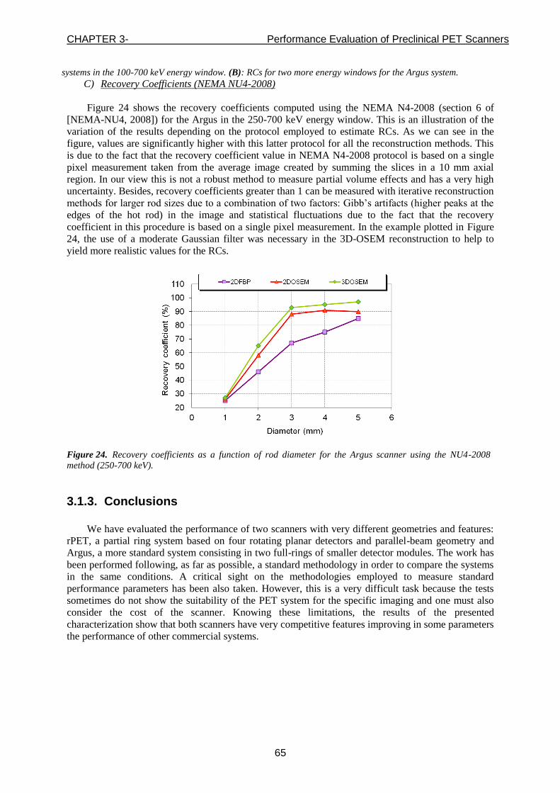
CHAPTER 3- Performance Evaluation of Preclinical PET Scanners
65
systems in the 100-700 keV energy window. (B): RCs for two more energy windows for the Argus system.
C) Recovery Coefficients (NEMA NU4-2008)
Figure 24 shows the recovery coefficients computed using the NEMA N4-2008 (section 6 of
[NEMA-NU4, 2008]) for the Argus in the 250-700 keV energy window. This is an illustration of the
variation of the results depending on the protocol employed to estimate RCs. As we can see in the
figure, values are significantly higher with this latter protocol for all the reconstruction methods. This
is due to the fact that the recovery coefficient value in NEMA N4-2008 protocol is based on a single
pixel measurement taken from the average image created by summing the slices in a 10 mm axial
region. In our view this is not a robust method to measure partial volume effects and has a very high
uncertainty. Besides, recovery coefficients greater than 1 can be measured with iterative reconstruction
methods for larger rod sizes due to a combination of two factors: Gibb’s artifacts (higher peaks at the
edges of the hot rod) in the image and statistical fluctuations due to the fact that the recovery
coefficient in this procedure is based on a single pixel measurement. In the example plotted in Figure
24, the use of a moderate Gaussian filter was necessary in the 3D-OSEM reconstruction to help to
yield more realistic values for the RCs.
Figure 24. Recovery coefficients as a function of rod diameter for the Argus scanner using the NU4-2008
method (250-700 keV).
3.1.3. Conclusions
We have evaluated the performance of two scanners with very different geometries and features:
rPET, a partial ring system based on four rotating planar detectors and parallel-beam geometry and
Argus, a more standard system consisting in two full-rings of smaller detector modules. The work has
been performed following, as far as possible, a standard methodology in order to compare the systems
in the same conditions. A critical sight on the methodologies employed to measure standard
performance parameters has been also taken. However, this is a very difficult task because the tests
sometimes do not show the suitability of the PET system for the specific imaging and one must also
consider the cost of the scanner. Knowing these limitations, the results of the presented
characterization show that both scanners have very competitive features improving in some parameters
the performance of other commercial systems.

CHAPTER 3- Performance Evaluation of Preclinical PET Scanners
66
3.2. Scatter Fraction estimation using 18
F and 68
Ga sources
As it was mentioned in section 3.1.1.4, the scatter fraction (SF) in PET data represents the
fraction of coincidence events in which at least one of the two emitted photons have been scattered
before being detected. Scattered events decrease image contrast in PET by misplacing events during
reconstruction, and cause errors in the reconstructed radioactivity concentration. Scatter can arise from
three major sources: scatter inside the object, detector backscatter, and scatter from the gantry and
surrounding environment. A good understanding of the contributions from the three sources is
essential to accurately correct for scatter in PET imaging.
In this section we present an evaluation of the procedure proposed by NEMA (section 4 of
[NEMA-NU4, 2008]) to estimate SF with 18
F. Further, we study the case of employing 68
Ga for this
estimation. The main advantage of 68
Ga over 18
F is that it can be obtained on-site, since it is extracted
from a gallium-68 generator, and a cyclotron is not necessary and it is becoming increasingly
employed. However 68
Ga is a radionuclide with lager positron range and this fact may have an impact
in the determination of scatter fraction and other performance parameters. We will try to see whether
using the same protocols as with 18
F, the values obtained can be compared to the ones determined from 18
F acquisitions [Vicente et al., 2010a].
For this study, experimental data acquired with the Argus small-animal PET scanner ([Wang et
al., 2006b], section 2.2) as well as peneloPET simulations ([España et al., 2009], section 2.3) are used.
3.2.1. Materials & Methods
3.2.1.1. Real and simulated data
In order to estimate SF with the protocol proposed by NEMA (section 4 of [NEMA-NU4, 2008]),
real data acquired with the Argus small-animal PET scanner (see section 2.2) as well as simulations of
the same scanner using peneloPET (see section 2.3), were used. The results were obtained using the
mouse sized phantom (see Appendix A) and a wide energy window (100-700 keV). The activity in the
line source inserted in the phantom was low to ensure that the number of random counts was
negligible (less than 1% of true rates). Simulated data were obtained with and without scanner
shielding and animal bed materials.
Figure 25. Diagram of Argus PET/CT and phantom.
An accurate simulation of the positron range, taking into account the small region of air between
the line source tube and the polyethylene phantom, was necessary to reproduce the width of the line
source profiles measured for both radionuclides, especially in the case of the 68
Ga.
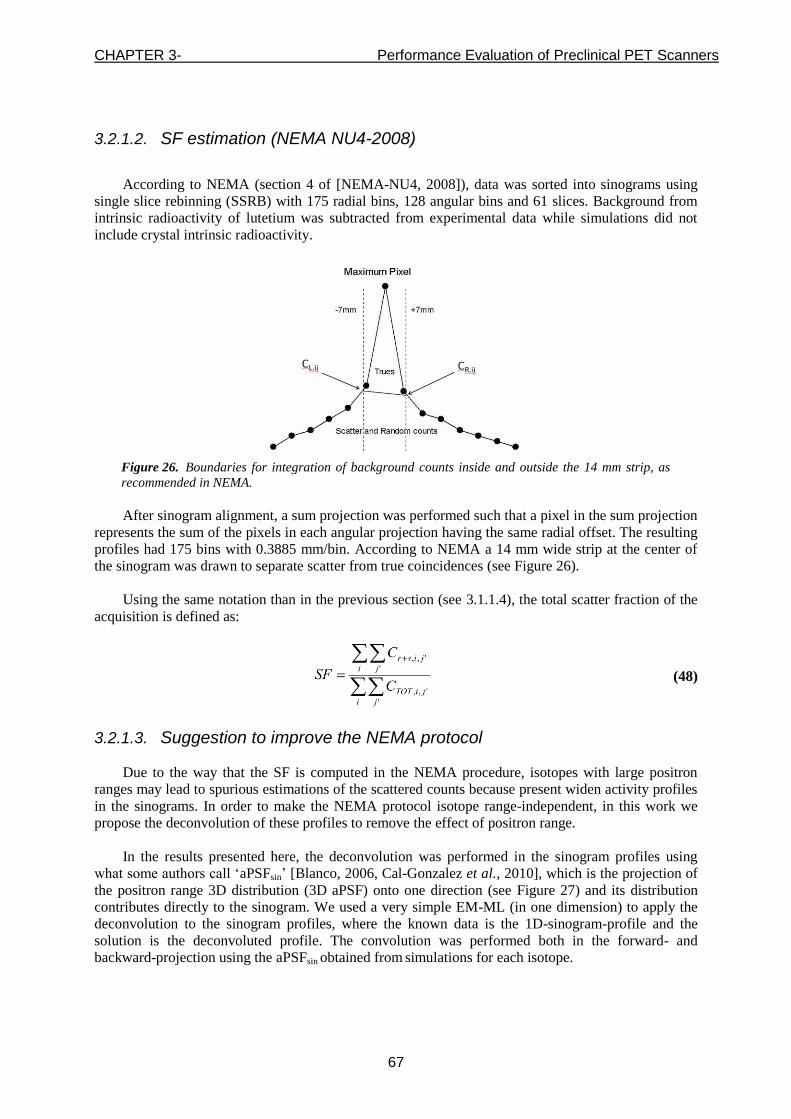
CHAPTER 3- Performance Evaluation of Preclinical PET Scanners
67
3.2.1.2. SF estimation (NEMA NU4-2008)
According to NEMA (section 4 of [NEMA-NU4, 2008]), data was sorted into sinograms using
single slice rebinning (SSRB) with 175 radial bins, 128 angular bins and 61 slices. Background from
intrinsic radioactivity of lutetium was subtracted from experimental data while simulations did not
include crystal intrinsic radioactivity.
Figure 26. Boundaries for integration of background counts inside and outside the 14 mm strip, as
recommended in NEMA.
After sinogram alignment, a sum projection was performed such that a pixel in the sum projection
represents the sum of the pixels in each angular projection having the same radial offset. The resulting
profiles had 175 bins with 0.3885 mm/bin. According to NEMA a 14 mm wide strip at the center of
the sinogram was drawn to separate scatter from true coincidences (see Figure 26).
Using the same notation than in the previous section (see 3.1.1.4), the total scatter fraction of the
acquisition is defined as:
(48)
3.2.1.3. Suggestion to improve the NEMA protocol
Due to the way that the SF is computed in the NEMA procedure, isotopes with large positron
ranges may lead to spurious estimations of the scattered counts because present widen activity profiles
in the sinograms. In order to make the NEMA protocol isotope range-independent, in this work we
propose the deconvolution of these profiles to remove the effect of positron range.
In the results presented here, the deconvolution was performed in the sinogram profiles using
what some authors call ‘aPSFsin’ [Blanco, 2006, Cal-Gonzalez et al., 2010], which is the projection of
the positron range 3D distribution (3D aPSF) onto one direction (see Figure 27) and its distribution
contributes directly to the sinogram. We used a very simple EM-ML (in one dimension) to apply the
deconvolution to the sinogram profiles, where the known data is the 1D-sinogram-profile and the
solution is the deconvoluted profile. The convolution was performed both in the forward- and
backward-projection using the aPSFsin obtained from simulations for each isotope.

CHAPTER 3- Performance Evaluation of Preclinical PET Scanners
68
Figure 27. Schematic procedure to obtain aPSFsin and aPSFimg from the original 3D aPSF [Cal-Gonzalez et
al., 2010].
3.2.2. Results
3.2.2.1. Experimental results
In Figure 28, 18
F and 68
Ga sinogram profiles for low activity concentrations are compared for
experimental acquisitions. It can be observed a wider line source profile for 68
Ga due to the positron
range effect.
Figure 28. 18F and
68Ga radial profiles for experimental acquisitions in the ARGUS system.
Y-axis is in logarithmic scale. Profiles are normalized dividing by the total counts of the
profile
Profiles were normalized dividing by the total counts of the profile. The two vertical lines show
the edges of the 14 mm wide strip which was used to estimate, using the NEMA NU4-2008 protocol,
the scatter coincidences distribution or ‘scatter (NEMA)’ as we call it in this work. This ‘scatter
(NEMA)’ is shown in the plot using dashed lines, and reported in Table 16 for both isotopes. We can
see that the SF value obtained using 68
Ga is higher than using 18
F. However, the SF is the same for
both isotopes, as we can see from the results of the simulations (Table 17, third column), where the
scatter fraction is computed from the actual scatter counts, known in a simulation, instead from
estimations as in the real case. The increased width of the 68
Ga profile due to positron range leads to a
spurious estimation of the fraction of scattered counts because contributions coming from the tail of
the profile of true counts contaminate the ‘scatter region’ defined by NEMA.

CHAPTER 3- Performance Evaluation of Preclinical PET Scanners
69
Table 16. Scatter Fraction values for real data using NEMA NU4-2008 protocol
Isotope SF (%) (NEMA)
18F 28
68Ga 35
3.2.2.2. Analysis using simulations
(A) (B)
Figure 29. Radial profiles of positron annihilation events in water and in water plus the observed air gap.
(A): 18
F isotope. (B): 68
Ga isotope.
Figure 29 shows the radial profiles of positron range in water and in water plus the observed air
gap in the experimental setup in between the capillary tube and the phantom. These profiles were used
in the simulations.
Figure 30 and Figure 31 show a comparison between real and simulated data (with and without
scanner shields and two different positron range profiles (Figure 29)) for 18
F (Figure 30) and 68
Ga
(Figure 31) respectively. For each plot, it is shown, besides the sinogram profiles of the total number
of coincidences (red and blue solid lines for real and experimental data respectively), the scatter
estimation using the NEMA method (scatter (NEMA), purple and orange dashed lines for real and
experimental data respectively), and the scatter estimated from the simulation (scatter (in sim.), green
dashed line).

CHAPTER 3- Performance Evaluation of Preclinical PET Scanners
70
Differences between simulations (with shields and realistic positron range) and real data are
probably due to additional shields not considered in the simulation. We did not find these differences
in the rPET scanner as it is shown in [España et al., 2009]. Despite these differences, simulated data
reveal interesting results:
Simulated sinogram profiles in left plots (A and C) were performed using simulations of
positron range in water. On the other side, right plots (B and D) were performed using a more
realistic simulation of the positron range which took into account the air gap in between the
capillary tube and the phantom (water plus a thin air layer). No significant differences are
observed in 18
F profiles (Figure 30), however, the 68
Ga profile using ‘water plus a thin air layer
positron range simulation’ resembles more closely the experimental profile (Figure 31D).
Taking into account the contribution from the shields, plots in the upper side (A and B) were
simulated without shields, while in the bottom plots (C and D) an approximation of the gantry
and the environment surrounding the scanner (what we call ‘shields’) were introduced in the
simulation. Flat scatter profiles are the result of having no shield as we can see in the green
dashed line profiles in both Figure 30 and Figure 31, A and B. Nevertheless, peaked profiles
are obtained for both isotopes when shields are a simulated. This peak (close to the line source
location) is due to low angle scatter at the shields.
Figure 30. 18F radial profiles for real acquisitions compared to different simulations: (A): Scanner without
shields. Positron range in water. (B): Scanner without shields. Positron range in water plus a thin air layer.
(C): Scanner with shields. Positron range in water. (D): Scanner with shields. Positron range in water plus a
thin air layer.
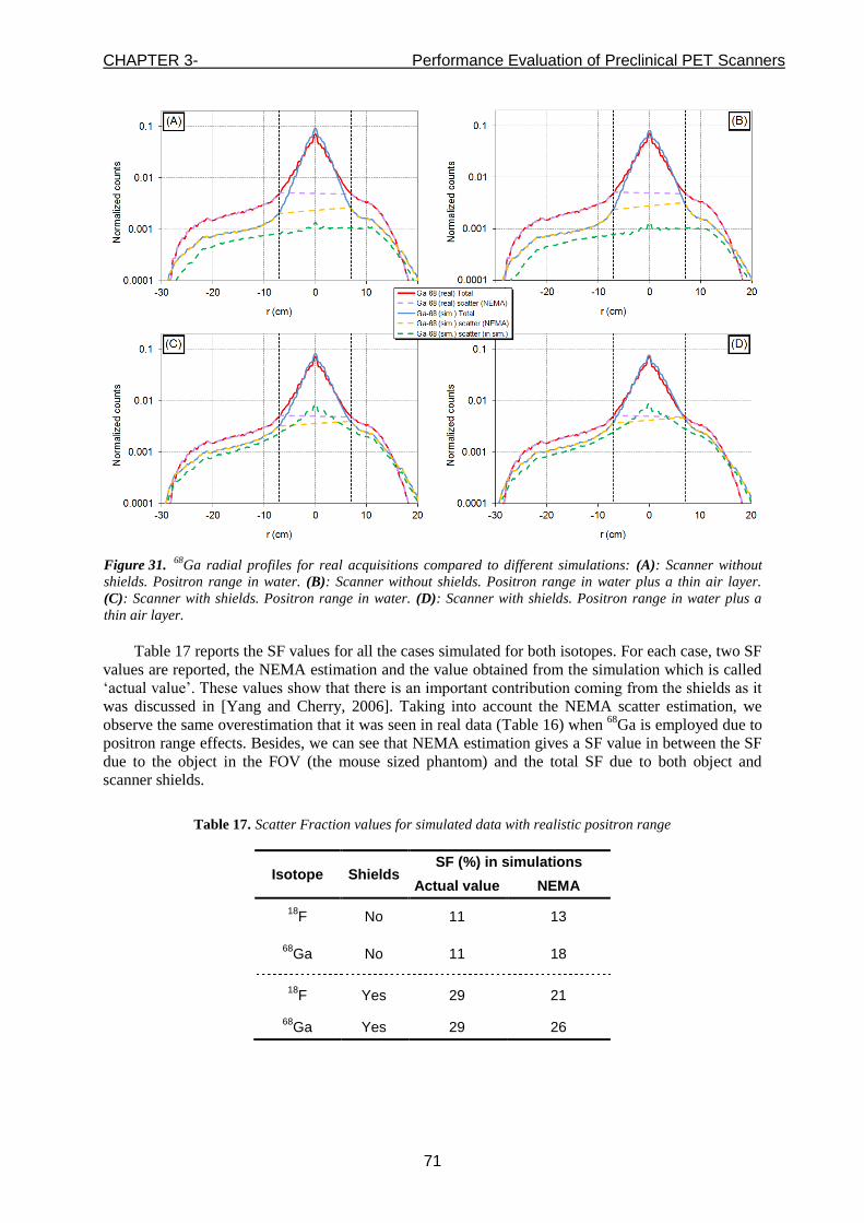
CHAPTER 3- Performance Evaluation of Preclinical PET Scanners
71
Figure 31. 68Ga radial profiles for real acquisitions compared to different simulations: (A): Scanner without
shields. Positron range in water. (B): Scanner without shields. Positron range in water plus a thin air layer.
(C): Scanner with shields. Positron range in water. (D): Scanner with shields. Positron range in water plus a
thin air layer.
Table 17 reports the SF values for all the cases simulated for both isotopes. For each case, two SF
values are reported, the NEMA estimation and the value obtained from the simulation which is called
‘actual value’. These values show that there is an important contribution coming from the shields as it
was discussed in [Yang and Cherry, 2006]. Taking into account the NEMA scatter estimation, we
observe the same overestimation that it was seen in real data (Table 16) when 68
Ga is employed due to
positron range effects. Besides, we can see that NEMA estimation gives a SF value in between the SF
due to the object in the FOV (the mouse sized phantom) and the total SF due to both object and
scanner shields.
Table 17. Scatter Fraction values for simulated data with realistic positron range
Isotope Shields SF (%) in simulations
Actual value NEMA
18F No 11 13
68Ga No 11 18
18F Yes 29 21
68Ga Yes 29 26

CHAPTER 3- Performance Evaluation of Preclinical PET Scanners
72
3.2.2.3. Suggestion to improve the NEMA protocol
Table 16 and Table 17 show that the NEMA protocol overestimates the SF for 68
Ga due to its
large positron range. In order to make the NEMA protocol isotope range-independent, in this work we
propose the deconvolution of the radial profiles to remove the effect of positron range from the profile
(Figure 32).
Figure 32. 68Ga (left) and
18F (right) radial profiles and SF values with and without positron range correction
The results of the NEMA SF values with and without positron correction for both isotopes are
shown in Table 18. We can see that for 18
F there are not differences in SF values with and without the
correction but SF for 68
Ga provides the same value than 18
F after positron range correction. Correcting
the profiles for range effect (a relatively simple procedure), would allow using isotopes with relatively
large range together with the NEMA protocol.
Table 18. Scatter Fraction values for simulated data with and without positron range correction
Isotope Range correction SF (%) (NEMA)
68Ga
No 26
Yes 21
18F
No 21
Yes 21
3.2.3. Conclusions
Positron range corrections are necessary if isotopes with significantly large positron range (as 68
Ga) are used to estimate the SF using the NEMA protocol.
Simulations show that scatter profiles are quite flat when no shields are taken into account, which
means that the scatter coming from the object produces a relatively flat count distribution background.
On the other hand, peaked scatter profiles (with the peak close to the line source location) are observed
when shields are simulated, having the scatter in the shields a very important contribution to the total
scatter fraction. In order to reproduce adequately the experimental data, simulations should model
shields accurately. Counts scattered on the shields would be taken for true counts when analyzed in

CHAPTER 3- Performance Evaluation of Preclinical PET Scanners
73
terms of the NEMA SF protocol, which was designed assuming a flat scatter background. This seems
to be the main reason for the underestimation of the total SF in the NEMA NU4-2008 protocol.
Results obtained with this method yield a value in between the SF due to the object solely and the total
SF due to the object and the scanner shields.
As a summary of this chapter, we have argued for the importance of standardized protocols to
assess the performance of scanner systems and used them to compare two PET scanners between them
and to other scanners available on the market. We have also shown that we should be aware that these
protocols are not flawless. We have analyzed in detail some examples and, with the help of very
detailed and realistic simulations, we have been able to propose improvements to these protocols.

CHAPTER 3- Performance Evaluation of Preclinical PET Scanners
74
3.3. References Bailey, D. L. 2005. Positron emission tomography: basic sciences, Springer.
Bailey, D. L., Jones, T., Spinks, T. J., Gilardi, M.-C. & Townsend, D. W. 1991. Noise equivalent count measurements in a
neuro-PET scanner with retractable septa. IEEE Trans. Med. Imaging, 10, 256-60.
Bao, Q., Newport, D., Chen, M., Stout, D. B. & Chatziioannou, A. F. 2009a. Performance evaluation of the inveon dedicated
PET preclinical tomograph based on the NEMA NU-4 standards. J Nucl Med, 50, 401-8.
Cherry, S. R., Sorenson, J. A. & Phelps, M. E. 2003. Physics in nuclear medicine, Saunders.
Del Guerra, A., Bartoli, A., Belcari, N., Herbert, D., Motta, A., Vaiano, A., Di Domenico, G., Sabba, N., Moretti, E.,
Zavattini, G., Lazzarotti, M., Sensi, L., Larobina, M. & Uccelli, L. 2006. Performance evaluation of the fully
engineered YAP-(S)PET scanner for small animal imaging. Nuclear Science, IEEE Transactions on, 53, 1078-
1083.
España, S., Herraiz, J. L., Vicente, E., Vaquero, J. J., Desco, M. & Udias, J. M. 2009. PeneloPET, a Monte Carlo PET
simulation tool based on PENELOPE: features and validation. Phys Med Biol, 54, 1723-42.
Goertzen, A. L., Bao, Q., Bergeron, M., Blankemeyer, E., Blinder, S., Cañadas, M., Chatziioannou, A. F., Dinelle, K.,
Elhami, E., Jans, H.-S., Lage, E., Lecomte, R., Sossi, V., Surti, S., Tai, Y.-C., Vaquero, J. J., Vicente, E., Williams,
D. A. & Laforest, R. 2012. NEMA NU 4-2008 Comparison of Preclinical PET Imaging Systems. The Journal of
Nuclear Medicine (Accepted).
Kisung, L., Kinahan, P. E., Miyaoka, R. S., Jae-Seung, K. & Lewellen, T. K. 2004. Impact of system design parameters on
image figures of merit for a mouse PET scanner. Nuclear Science, IEEE Transactions on, 51, 27-33.
Knoess, C., Siegel, S., Smith, A., Newport, D., Richerzhagen, N., Winkeler, A., Jacobs, A., Goble, R. N., Graf, R., Wienhard,
K. & Heiss, W. D. 2003. Performance evaluation of the microPET R4 PET scanner for rodents. Eur J Nucl Med
Mol Imaging, 30, 737-47.
Levin, C. S., Foudray, A. M. K. & Habte, F. 2006. Impact of high energy resolution detectors on the performance of a PET
system dedicated to breast cancer imaging. Physica Medica, 21, 28-34.
National Electrical Manufacturers Association (NEMA). 1994. Performance Measurements of Positron Emission
Tomographs. NEMA Standards Publication NU2-1994. Rosslyn, VA. National Electrical Manufacturers
Association
National Electrical Manufacturers Association (NEMA). 2001. Performance Measurements of Positron Emission
Tomographs. NEMA Standards Publication NU2-2001. Rosslyn, VA. National Electrical Manufacturers
Association
National Electrical Manufacturers Association (NEMA). 2008. Performance Measurements of Small Animal Positron
Emission Tomographs. NEMA Standards Publication NU4-2008. Rosslyn, VA. National Electrical Manufacturers
Association
Strother, S. C., Casey, M. E. & Hoffman, E. J. 1990. Measuring PET scanner sensitivity: relating countrates to image signal-
to-noise ratios using noise equivalents counts. Nuclear Science, IEEE Transactions on, 37, 783-788.
Surti, S., Karp, J. S., Perkins, A. E., Cardi, C. A., Daube-Witherspoon, M. E., Kuhn, A. & Muehllehner, G. 2005. Imaging
performance of a-PET: a small animal PET camera. Medical Imaging, IEEE Transactions on, 24, 844-852.
Tai, C., Chatziioannou, A., Siegel, S., Young, J., Newport, D., Goble, R. N., Nutt, R. E. & Cherry, S. R. 2001. Performance
evaluation of the microPET P4: a PET system dedicated to animal imaging. Phys Med Biol, 46, 1845-62.
Vaquero, J. J. & Desco, M. 2005. Limitaciones tecnológicas de la tomografía por emisión de positrones (PET) para pequeños
animales de laboratorio. [Technical limitations of the positron emission tomography (PET) for small laboratory
animals]. Rev Esp Med Nucl, 24, 334-47.
Vaquero, J. J., Lage, E., Ricón, L., Abella, M., Vicente, E. & Desco, M. 2005b. rPET Detectors Design and Data Processing.
IEEE Nuclear Science Symposium Conference Record.
Vicente, E., Herraiz, J. L., Canadas, M., Cal-Gonzalez, J., Espana, S., Desco, M., Vaquero, J. J. & Udias, J. M. 2010a.
Validation of NEMA NU4-2008 Scatter Fraction estimation with 18F and 68Ga for the ARGUS small-animal PET
scanner. In: Nuclear Science Symposium Conference Record (NSS/MIC), 2010 IEEE, Oct. 30 2010-Nov. 6 2010
2010a. 3553-3557.
Vicente, E., Vaquero, J. J., Lage, E., Tapias, G., Abella, M., Herraiz, J. L., España, S., Udías, J. M. & Desco, M. 2006
Caracterización del Tomógrafo de Animales rPET. Libro de Actas, CASEIB 2006.
Wang, Y., Seidel, J., Tsui, B. M., Vaquero, J. J. & Pomper, M. G. 2006b. Performance evaluation of the GE healthcare
eXplore VISTA dual-ring small-animal PET scanner. J Nucl Med, 47, 1891-900.
Weber, S. & Bauer, A. 2004. Small animal PET: aspects of performance assessment. Eur J Nucl Med Mol Imaging, 31, 1545-
55.
Yang, Y. & Cherry, S. R. 2006. Observations regarding scatter fraction and NEC measurements for small animal PET.
Nuclear Science, IEEE Transactions on, 53, 127-132.

CHAPTER 4- Data-Corrections in Preclinical PET
75
4. Data-Corrections in Preclinical PET
As it was introduced in chapter 1, (section 1.3), in order to provide quantitative images from PET
scanners, the data must be processed taking into account physical effects such as attenuation, scatter,
or decay time of the radioactive source. Furthermore, the scanner electronics produces random counts,
pile-up and dead-time effects, and the efficiency of individual detector elements as well as the exact
geometry of the scanner may differ slightly from the ideal expectation, due to statistical variations in
the properties of the detectors and unavoidable variations during construction of scanner and detector
elements. All of these effects cause the scanner to depart from the ideal behavior and they must be
taken into account to reproduce a linear relation between tracer activity in the scanner and activity
measured.
In this chapter we study in detail some of these corrections, with examples taken from the two
scanners whose performance evaluations were presented in the previous chapter, but they can be also
applied to other systems. In section 4.1we introduce a novel method to take into account pile-up and
dead-time effects. Section 4.2 presents a quantitative study of the effect on the image quality of small
mechanical misalignments in rotating PET systems made of planar detectors and a calibration protocol
to correct for them. This later correction was not described in chapter 1 since it is not such a usual
correction in PET systems as it is for CT and SPECT scanners. Finally, in section 4.3 we describe an
attenuation correction method based on CT images. This is a rather standard implementation based on
previous works, but we wanted to include it in this thesis as an example of the software developed by
our group and that is being commercialized as part of the reconstruction software for the Argus
System.
CHAPTER 4- Data-Corrections in Preclinical PET
76
4.1. Modeling of pile-up and dead-time for small animal PET scanners
In a photon detector system, pile-up occurs when a photon deposits energy in the detector while
the signal from a previous event is still being integrated [Knoll, 2000]. Pile-up effects are more
significant at high count rates. They become increasingly important when large-area detectors are used
[Mankoff et al., 1989, Smith et al., 1994, Vicente et al., 2007, Vicente et al., 2008], where every
channel of the electronic acquisition system is employed to read a substantial detector area, making the
possibility of achieving high count rates per electronic channel more likely.
Pile-up events induce two kinds of errors in PET data [Furrer et al., 1984]. On one hand, they
worsen resolution and contrast in detection systems which employ position sensitive block detectors
(either pixelated or monolithic) when they are read with multiplexed electronics using analog logic to
identify the position of interaction. If additional photons reach the detector after the trigger event and
during the integration time, they will be processed along with the photon which originated the trigger
as part of the same single event. For these pile-up events, the apparent location of the interaction will
be inaccurate and, if they are not rejected, will cause miss-positioning of coincidence events [Germano
and Hoffman, 1990, Badawi and Marsden, 1999b].
Figure 33C shows the distribution of pile-up events at high activity (2400 Ci in the Field of
View (FOV)) in a simulated flood histogram for a Hamamatsu H8500 flat-panel PS-PMT coupled to
an array of 28×28 LYSO crystals irradiated with a uniform source. Pile-up events would yield energy
to two different crystals of the same detectors. One can easily show that if we pick two crystals at
random and draw the mid-point of the segment joining both crystals, this mid-point tends to be located
on average at the central region of the surface of the detector. Thus, when there is noticeable pile-up in
the acquisition, the distribution of counts recorded in the detector tends to concentrate in the central
crystals of the array. At low activities (Figure 33, A and B), where pile-up is not significant, the count
distribution is uniform.
On the other hand, if the pile-up event provides a signal large enough to fall beyond the Upper
Level Discriminator (ULD) of the energy window employed in the acquisition, the event will be
rejected. When this happens, the number of coincidences acquired is reduced and consequently the
count statistics of the image. Moreover, as pile-up is a non-linear effect, if it is not taken into account,
quantification may be compromised.
In Figure 33D energy spectra for the same three acquisitions above-mentioned are shown.
Profiles are normalized to the same number of coincidences. The spectra for low activities (dotted and
light-color curves) are quite similar, but we can see in the 240 Ci spectrum a lower photopeak height
and a slight excess of counts around the 1022 keV peak, corresponding to the pile-up of two photons
of 511 keV each one. At 2400 Ci (dark line), count losses at the photopeak and below 200 keV are
very important and there is an evident excess of counts above the photopeak, due to all the photon
pile-up combinations, having the 1022 keV peak higher probability.

CHAPTER 4- Data-Corrections in Preclinical PET
77
(A) (B)
(C) (D)
Figure 33. (A), (B) and (C): Simulated flood histogram for a Hamamatsu H8500 flat-panel PS-PMT
coupled to an array of 28×28 LYSO crystals with 24, 240 and 2400 Ci inside the FOV, respectively.
(D): Energy spectra for the same three activities. Profiles are normalized to the same number of
coincidences.
We classify in more detail, as a function of the effect within the energy window used, the
different situations that may arise when one of the two singles of a coincidence is affected by pile-up.
Let E1 and E2 be the energy of each photon of the pile-up event (assuming pile-up of 2 photons) and
LLD and ULD the Lower and Upper Level Discriminators of the energy window respectively. Let us
assume that the photon with energy E1 is the one which is in true coincidence (before filtering by the
energy window) with another photon (E3 [LLD, ULD], for simplicity). We can distinguish three
cases, as shown in Table 19, with regard to the effect of pile-up in the count rate:
Table 19. Classification of pile-up events.
CASE 1
LLDEE 21
CASE 2
ULDEELLD 21
CASE 3
21 EEULD
A) E1 < LLD No effect Coincidence gain.
Distorted position and energy information
No effect
B) E1 [LLD,ULD] --- No Coincidence gain.
Distorted position and energy information
Coincidence loss
C) E1 > ULD --- --- No effect
There are different ways to reduce pile-up effects at the hardware level [Smith et al., 1994]. One
way is to use the shortest possible integration time to reduce the probability of pile-up. But integration
time cannot be arbitrarily short since enough light has to be integrated to keep acceptable spatial and

CHAPTER 4- Data-Corrections in Preclinical PET
78
energy resolutions. This measure relies on finding scintillators with shorter light decay times. Another
way to reduce the effect of pile-up on the count rate capability of the system is to use a restricted
energy window. Another method is increasing the number of electronic channels which read the
detectors, so that the count rate associated to every electronic channel is reduced, for the same count
rate in the dectector. Further methods to reject pile-up events can be found, for example, in [Germano
and Hoffman, 1991, Sjöland and Kristiansson, 1994, Imperiale and Imperiale, 2001]. Pile-up rejection
mechanisms can significantly reduce the spectral distortions associated to pile-up, but count losses
must be still corrected in the quantitative analysis.
The count rate in a PET scanner as a function of the activity in the Field of View (FOV) has non-
linear contributions coming not only from pile-up, but also from dead-time and random coincidences [Knoll, 2000, Cherry et al., 2003]. An accurate estimation of these non-linear effects is essential for
quantitative PET studies [Bendriem and Townsend, 1998]. Methods to estimate and correct the effects
of random coincidences in PET studies can be found in [Knoll, 2000, Williams et al., 1979, Casey and
Hoffman, 1986, Badawi et al., 1999, Stearns et al., 2003, Brasse et al., 2005]. In this work we focus
on pile-up and dead-time effects, what we call ‘effective dead-time’, as they are closely related. By
dead-time we refer to the loss of counts due to the inability of detectors, electronics, computer disk and
software, or any other part of the signal chain, of processing all physical valid events because the
system is busy processing a previous event. In a sense, pile-up, when causing loss of counts, can be
considered as an ingredient of a general dead-time concept. Such is the case that it is often found in the
literature that both dead-time and pile-up effects are referred to simply as dead-time.
Several methods for characterizing the count rates of a PET scanner and data losses due to pile-up
and dead-time effects have been proposed. For instance, in Hoffman et al. [1983], corrections for
dead-time loss are calculated from the ‘on-line’ measurement of triple coincidence events. Stearns et
al. [1985] measured dead-time losses for both single events and total coincidence events independently
to obtain the total dead-time. Mazoyer et al. [1985] proposed a scheme which was based on the
paralyzing dead-time model using the total coincidence rate correcting both, the emission and
transmission data (used for attenuation correction). Yamamoto et al. [1986] proposed a method to
correct dead-time using a nonlinear function of the ‘off-line’ measured random coincidences. They
showed that the dead-time is a function of the object size as is the random count rate. Daube-
Witherspoon et al. model [1991], for emission and transmission 2D PET scanners, takes into account
coincidence losses due to singles losses and multiple events, as well as misspositioning errors at higher
count rates caused by pulse pile-up within a detector block. Eriksson et al. [1994] model assumes that
data losses can be factorized into two components, one part coming from the detector processing
system and one part coming from the data processing system.
As it can be seen from these examples, corrections of count losses due to dead-time and pile-up is
usually derived from a combination of analytical models that describe the individual electronics
components and empirical data derived from scanning phantoms at various input count rates. Dead-
time models usually treat system dead-time as being separable into two components, paralyzable and
non-paralyzable [Knoll, 2000].
Nevertheless, to the best of our knowledge, there are no simple protocols to estimate and to take
into account pile-up effects valid for a general acquisition since it depends on the material and object
size placed in the FOV and the source distribution (inside/outside the FOV) because it changes the
ratio between the number of coincidences and the number of singles. This means that the
quantification properties of images obtained from high-activity acquisitions (with large pile-up effects)
are usually compromised by pile-up effects. In the method outlined by Yamamoto et al. [1986] this is
taken into account, but in their procedure it is necessary to measure the ‘off-line’ random
coincidences, which is not always possible or practical.
In this work [Vicente et al., 2012a, Vicente et al., 2011] we propose to use an effective dead-time,
, which can be easily computed for any acquisition and scanner, and linearizes the dependence of the
count rates with the activity. This effective dead-time takes into account pile-up losses and gains and

CHAPTER 4- Data-Corrections in Preclinical PET
79
dead-time losses. The method requires only two calibration acquisitions and is based on the linear
relationship between and the Singles-to-Coincidences ratio (SCR). We have verified that the method
is valid even when the effects of pile-up are important, as it is the case of one of the scanners used in
this study, rPET [Vaquero et al., 2005b], with large area detectors and without electronic pile-up
rejection. We present results for this specific scanner, but the method was also applied to other
systems, such as SEDECAL Argus scanner (formerly GE eXplore Vista) [Wang et al., 2006b],
demonstrating its applicability.
4.1.1. Materials & Methods
4.1.1.1. Count rate linearization
The decaying source method to estimate the effective dead-time
Dead-time behaviour in a PET scanner as a function of the count rate is often estimated by means
of a decaying source experiment [Knoll, 2000]. Repeated measurements of total coincidence rates are
obtained for different activities of a decaying source. In the limit of very low activities, when dead-
time (and other nonlinear effects) vanishes, the measured count rate, m(t), would coincide with the true
incident count rate n(t). Since the true incident count rate for larger activities can be easily calculated
according to the decay time correction, the ratio of incident to measured counts ([m(t)]d /[n(t)]d, where
the subscript d stands for decay corrected) can be estimated for any activity. This allows to obtain
empirically a dead-time correction for a given acquisition and scanner. It is a common procedure to fit
this dead-time correction factor [m(t)]d /[n(t)]d to an analytic expression containing an effective dead-
time , using either paralyzable, non paralyzable or mixed models [Knoll, 2000].
Sometimes dead-time corrections for a given scanner are obtained by means of a reference
acquisition of an intermediate size phantom [Knoll, 2000, Germano and Hoffman, 1988]. Once the
effective dead-time is obtained from this phantom, corrections evaluated with the same value of are applied to all acquisitions performed by the same scanner. In what follows, we refer to this method
as ‘single-parameter method’.
New method to estimate effective dead-times: the SCR-based method
Yamamoto et al [1986] and Thompson and Meyer [1987] studied the dependence of on the size
of the object in the FOV. We deepened on this study, performing simulations of decaying sources with
different materials and sizes of the phantoms, and different energy windows for the acquisition. Table
20 summarized the simulated phantoms used, ranging from point sources to capillary sources in
cylinders of different materials and sizes. The effective dead-time for each phantom acquisition was
obtained with the decaying source method explained in the previous section. We expected these
effective dead-time values to depend on the Singles-to-Coincidences ratio (SCR) for each
acquisition. Thus, we plotted effective dead-times against the true SCR9 values for each acquisition.
By ‘true’ we mean SCR free from dead-time, pile-up and random count effects. These can be easily
obtained from a decaying source experiment in the limit of vanishing activity.
It can be shown that a linear relationship between the effective dead-time, , and the SCR exists
(see Appendix 4.1A). This relationship can be explained as the result of two contributions: a dead-time
involving only events from detected coincidences, C, and an additional dead-time which affects every
single event, irrespectively of whether it results or not in an actually detected coincidence, represented
by the singles effective dead-time, S, which accounts for pile-up effects. Namely the expression is:
9 No energy window was applied to measure the singles rates.

CHAPTER 4- Data-Corrections in Preclinical PET
80
Cs SCR 2 (49)
Thus, the method proposed is based on two parameters (C and S) unlike the single-parameter
presented in the previous section. We propose to correct for pile-up and dead-time using two
calibration acquisitions, one with high SCR and one with low SCR, in order to estimate the C and S,
parameters which can be used to compute the effective dead-time, , of any other acquisition
following equation (49)(See Figure 34). We call this procedure the ‘SCR-based method’.
Figure 34. Flowchart of the SCR-based method to obtain the effective dead-time correction.
Table 20. Description of the phantoms simulated. Notation: PS: point source; SC: small cylinder; LC: large
cylinder; LS: line source; C: cylinder; d: cylinder diameter in cm (d=[0.4, 1, 2, 3, 4, 5]); : cylinder diameter;
h: cylinder height.
Phantom Name
Descriptiona Dimensions
Source (Isotope:
18F)
Object Source
/ h (cm)
Object
/ h (cm)
PS Point source Water cubic box 0.05 / -- x = 1 y = 1 z = 1
Water (SC)
Small cylinder (SC)
Small water cylinder
0.9 / 6.5
0.9 / 6.5
Al (SC) Small aluminium cylinder 0.9 / 6.5
GSO (SC) Small GSO cylinder 0.9 / 6.5
Pb (SC) Small lead cylinder 0.9 / 6.5
Water (LC) Large cylinder
(LC) Large water cylinder 5.5 / 5.0 5.5 / 5.0
Water (SL&Cd) d=[0.4,1,2,3,4,5]
Line Source (LS)
Water cylinder (C)
0.2 / 0.4
d / 4.0
Al (SL&Cd) d=[0.4,1,2,3,4,5]
Aluminium cylinder (C) d / 4.0
aAll phantoms (sources and objects) are placed at the centre of the FOV
CHAPTER 4- Data-Corrections in Preclinical PET
81
Validation of the SCR-based method
In order to evaluate the method proposed to correct by dead-time and pile-up effects we first
analyzed the decaying source method using both real data and simulations for the Water (SC) phantom
acquired with the rPET scanner [Vaquero et al., 2005b]. In this work we assumed a non-paralyzable
behaviour, although similar results are achieved with paralyzable expressions when the values of the
dead-time correction factor are not extreme, as it is the case of the scanners analyzed in this work
under their usual operational ranges. We performed a decaying source experiment with the rPET
system using a small cylinder (SC) phantom (0.9 cm diameter, 6.5 cm length) filled with 18
F in water
(‘Water (SC)’) placed at the centre of the FOV of the scanner. For reference, although it is not needed
in the procedure, the initial activity was measured in a well-counter with an accuracy of ±5%. Several
consecutive acquisitions of 5 minutes with an energy window of 400-700 keV were taken, starting
from an initial activity of 900 Ci, with an activity concentration of 254.6 Ci/cc and a total count rate
of 130 kcps. Also, acquisitions of this source were simulated with PeneloPET [España et al., 2009]
mimicking the experimental setup. In the simulations, we used a coincidence dead-time of 1.6 s,
which includes the conversion time of the ADC and an integration time of 0.22 s, values which suit
rPET hardware. From the simulations it is possible to estimate the individual contributions to the total
effective dead-time that can be split into three components: strict dead-time (DT ), pile-up losses
(p(loss)) and pile-up gains (p(gain)), according to:
)gain(p)loss(pDT (50)
The simulated phantoms described in Table 20 were used to study and validate the SCR-based
method. The effective dead-time for each phantom acquisition was estimated with the decaying source
method. The SCR-based method was applied using the PS and the Water (LC) phantoms as the two
calibration experiments, for both scanners described in chapter 2: rPET [Vaquero et al., 2005b] and
Argus [Wang et al., 2006b] systems. Random counts in the Argus scanner were removed from the
acquisition prior to the analysis of data to compute . For the rPET scanner this was not necessary as
the fraction of random counts for this scanner was negligible.
We also estimated the error introduced when the effective dead-time obtained for a particular
phantom is employed to correct dead-time for another phantom with different SCR, that is, when the
single-parameter method is employed, comparing the results with the ones obtained correcting with
effective dead-times estimated with the SCR-based method.
Besides simulations, the relationship between and SCR for the rPET scanner was explored also
with real data. The Water (SC) and Water (LC) phantoms were used as calibration acquisitions for the
SCR-based method to calculate the calibration parameters, C and S from eq. (49). A further
acquisition of a Hot Derenzo phantom (see Appendix A) was employed to compare the value
obtained from the decaying source method and the one obtained using the computed C and S from
eq. (49) (SCR-based method).
4.1.1.2. Activity calibration with reference data (Calibration curve)
Ideally, activity calibration is accomplished by measuring a phantom containing a known,
homogeneous activity concentration determined from an external independent measurement, using a
well-counter for example [Cherry et al., 2003].
For the activity calibration of the rPET scanner, the Water (SC) phantom was used. The
acquisition was reconstructed with a 3D-OSEM algorithm [Herraiz et al., 2006a]. Images from all
frames were obtained. Several regions of interest (with a size of a few cc to prevent partial volume
effects) were chosen at different places in the interior of the cylinder and at different slices and the

CHAPTER 4- Data-Corrections in Preclinical PET
82
mean value and the statistical error were computed for each frame. The counts per cubic centimeter
and second (cps/cc) obtained were compared to the known specific activity (uCi/cc) in the inner region
of the cylinder and the data were fit to a linear calibration curve, looking for the proportionality
constant relating the specific rate measured in the image to the known specific activity for each frame.
A linear fit assumes that non-linear effects have been removed.
4.1.2. Results
4.1.2.1. Count rate linearization
(A) (B)
0
20
40
60
80
100
120
140
160
180
0 5 10 15 20 25 30 35
Activity (MBq)
To
tal co
un
t ra
te (
kcp
s)
.
Ideal
measured (w/o correc.)
w pile-up(G) correc.
w pile-up(G) + DT correc.
w pile-up(G) + DT + pile-up(L) correc.
Figure 35. (A): Linear fits employed to derive for the Water (SC) phantom using the rPET scanner with a 400-
700 keV energy window. The dead-time correction factor [m(t)]d/[n(t)]d is plotted against measured count rates,
exhibiting an approximate linear behaviour in the range considered. The effective is obtained from the slope.
(B): Simulated study showing the different contributions to effective dead-time for the same case shown in (A), as
a function of activity in the FOV.
Figure 35A shows the linear fits where the deacaing source method and the non-paralyzable
model were used to estimate the effective dead-time of the Water (SC) phantom for real and
simulated data for rPET scanner. The resulting values are reported in Table 21 In the case of the
simulation, it is possible to estimate the contributions: dead-time and pile-up losses and gains.
Equation (50) was used to yield the total and this value is compared with the one obtained from the
fit using the deacaing source method. Two main results are worth mentioning:
1) A very good agreement of the value of the fitted effective between the simulation and the
experimental data is seen.
2) For the simulation, the obtained from the fit using the non-paralyzable model and the one
computed from the dead-time and pile-up (losses and gains) contributions using Eq. (50) are in
good agreement. This result indicates the consistency of the parameters inputted in the
simulation and the use of Eq. (50) to compute the total effective dead time.
Figure 35B shows the count rates of the simulated Water (SC) phantom in the 400-700 keV
energy window and the different corrections applied as a function of actual activity in the FOV. No
random correction was applied since, as we can see in Figure 36A, the percentage of random counts is
less than 3% for all count rates considered. Figure 35B shows the suitability of the obtained effective since the corrected count rates do not show significant differences from the ideal curve for both high
and low count rates.
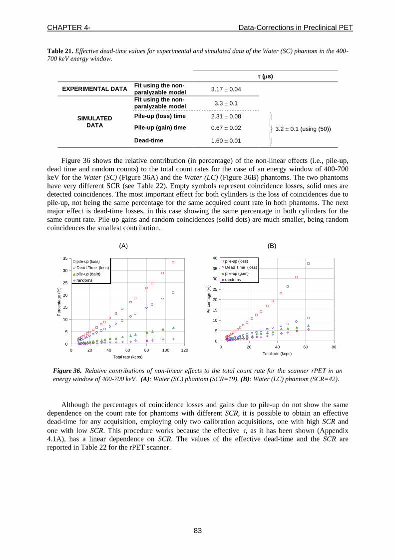
CHAPTER 4- Data-Corrections in Preclinical PET
83
Table 21. Effective dead-time values for experimental and simulated data of the Water (SC) phantom in the 400-
700 keV energy window.
(s)
EXPERIMENTAL DATA Fit using the non-paralyzable model
3.17 0.04
SIMULATED DATA
Fit using the non-paralyzable model
3.3 0.1
Pile-up (loss) time 2.31 0.08
3.2 0.1 (using (50)) Pile-up (gain) time 0.67 0.02
Dead-time 1.60 0.01
Figure 36 shows the relative contribution (in percentage) of the non-linear effects (i.e., pile-up,
dead time and random counts) to the total count rates for the case of an energy window of 400-700
keV for the Water (SC) (Figure 36A) and the Water (LC) (Figure 36B) phantoms. The two phantoms
have very different SCR (see Table 22). Empty symbols represent coincidence losses, solid ones are
detected coincidences. The most important effect for both cylinders is the loss of coincidences due to
pile-up, not being the same percentage for the same acquired count rate in both phantoms. The next
major effect is dead-time losses, in this case showing the same percentage in both cylinders for the
same count rate. Pile-up gains and random coincidences (solid dots) are much smaller, being random
coincidences the smallest contribution.
(A) (B)
0
5
10
15
20
25
30
35
0 20 40 60 80 100 120
Total rate (kcps)
Pe
rce
nta
ge
(%
)
pile-up (loss)
Dead Time (loss)
pile-up (gain)
randoms
0
5
10
15
20
25
30
35
40
0 20 40 60 80
Total rate (kcps)
Pe
rce
nta
ge
(%
)
pile-up (loss)
Dead Time (loss)
pile-up (gain)
randoms
Figure 36. Relative contributions of non-linear effects to the total count rate for the scanner rPET in an
energy window of 400-700 keV. (A): Water (SC) phantom (SCR=19), (B): Water (LC) phantom (SCR=42).
Although the percentages of coincidence losses and gains due to pile-up do not show the same
dependence on the count rate for phantoms with different SCR, it is possible to obtain an effective
dead-time for any acquisition, employing only two calibration acquisitions, one with high SCR and
one with low SCR. This procedure works because the effective , as it has been shown (Appendix
4.1A), has a linear dependence on SCR. The values of the effective dead-time and the SCR are
reported in Table 22 for the rPET scanner.

CHAPTER 4- Data-Corrections in Preclinical PET
84
1.5
2.0
2.5
3.0
3.5
4.0
4.5
5.0
5.5
0 10 20 30 40 50 60
SCR
rPE
T (
s)
0.5
0.6
0.7
0.8
0.9
1
1.1
1.2
1.3
rPET data
Argus data
Arg
us s)
Figure 37. Effective dead-time versus SCR for different acquisitions of rPET (diamonds, left Y axis) and Argus
(triangles, right Y axis) scanners (400-700 keV). The dashed line is a linear fit to all rPET points, and the solid
line is obtained from the two calibration points of the SCR-based method at the extreme values of SCR, namely
PS and Water (LC) phantoms in rPET. A similar line is also shown for the Argus scanner.
In Figure 37 we plot the effective dead-times obtained from simulations of the decaying
phantoms described in Table 20, for the case of the rPET scanner (diamonds), and for the Argus one
(triangles), against SCR. As expected, a linear behaviour is seen for both scanners. (Argus data results
are discussed at the end of this section). In this figure we also plot with solid lines the relationship
between the effective dead-time and the SCR estimated using our proposed SCR-based method using
two calibration acquisitions, namely the PS and the Water (LC) cylinder. These phantoms are
representative of both extreme sides of the SCR range. We used these two points to estimate the linear
relationship with SCR, although some points are slightly underestimated, because we found that an
error in the effective dead-time, , results in a lower error in the corrected count rates, n(t), when
< 0 (underestimation) than > 0 (overestimation). (For more details see Appendix 4.1B). The
calibration-estimated line lies slightly below the linear fit using all rPET phantoms (dashed line), but
with similar slope. The relative error between their intercept values is 6%. Despite this error in the
intercept, we found that using the SCR-based calibration method to compute each effective , the error
in the corrected count rate is less than 7%, even for high count rates, for all phantoms considered. An
example of this is shown in Figure 38.
Table 22. Singles-to-coincidence ratio (SCR) and effective dead-time () in the 400-700 keV energy window for
the simulated phantoms described in Table 20 for rPET scanner.
Phantom Name SCR (s) Phantom Name SCR (s)
PS 6.7 0.1 2.52 0.03 Water (SL&C3.0) 14.3 0.2 2.98 0.07
Water (SC) 19.0 0.3 3.4 0.1 Water (SL&C4.0) 15.5 0.3 3.22 0.08
Al (SC) 21.3 0.3 3.5 0.1 Water (SL&C5.0) 17.0 0.2 3.19 0.07
GSO (SC) 26.7 0.6 3.7 0.2 Al (SL&C0.4) 11.6 0.2 2.93 0.06
Pb (SC) 37 1 4.7 0.5 Al (SL&C1.0) 13.7 0.2 3.09 0.07
Water (LC) 42.4 0.7 4.6 0.2 Al (SL&C2.0) 17.3 0.3 3.5 0.1
Water (SL&C0.4) 10.9 0.2 2.86 0.05 Al (SL&C3.0) 21.6 0.4 3.6 0.1
Water (SL&C1.0) 11.7 0.2 2.97 0.05 Al (SL&C4.0) 26.4 0.7 3.8 0.2
Water (SL&C2.0) 13.0 0.2 2.98 0.06 Al (SL&C5.0) 31.2 0.7 4.0 0.2

CHAPTER 4- Data-Corrections in Preclinical PET
85
We show in Figure 38 a comparison between the single-parameter method (1-param. correction)
and the one proposed in this work (SCR-based method), for the rPET scanner in the 400-700 keV
energy window. For the single-parameter method, we used the Water (SC) phantom to get the fixed
value. In the figure we plot the ratios of corrected over ideal count rates for two situations: a point
source (PS) and the small cylinder of lead (Pb (SC)). The PS was chosen to show the magnitude of the
error in the corrected count rates when the effective dead-time is overestimated, as it happens when
using the dead-time obtained with the single-parameter method from the Water (SC) to correct the
count rates of the PS acquisition. The second example, Pb (SC), was selected because this is the point
with the worse fit to the calibration-estimated line for rPET scanner in the SCR-based method (see
Figure 37, point: (37, 4.7)). We can see that in both cases the SCR-based method provides more
accurate results, with a relative error smaller than 7% for the Pb (SC) phantom and less than 6% for
the PS, compared to deviations of 10% for the Pb (SC) phantom and even up to 100% (PS) when the
1-parameter correction is employed. This example shows that the 1-parameter correction introduces a
bias in the corrected count rates. This error is large if the used for the correction overestimates the
one of the acquisition and will be more significant for large detector blocks, so the SCR-based method
would be highly recommended for clinical dedicated-breast PET scanners (or PEM cameras) as for
example the ones described in [Wang et al., 2006a, Wu et al., 2009] or for high sensitivity preclinical
PET scanners with detectors particularly close as, for example the ones described in [Seidel et al.,
2010, Zhang et al., 2011].
0.80
0.90
1.00
1.10
1.20
1.30
1.40
1.50
1.60
1.70
1.80
1.90
2.00
2.10
0 5 10 15 20 25 30
Activity (MBq)
(Co
rr.
co
un
ts r
ate
) /
(Id
ea
l co
un
ts r
ate
s)
.
Pb (SC) [SCR-based method]
PS [SCR-based method]
Pb (SC) [1-param. correction]
PS [1-param. correction]
Figure 38. Comparison of the ratio of corrected over ideal rates for the SCR-based method (solid points) and
the single-parameter method which uses only one value for the effective dead-time (1-param. correction, empty
points) for the PS and the Pb (SC) phantoms. It can be observed that in both cases the SCR-based method
provides more accurate results, with a relative error smaller than 7% for the Pb (SC) phantom and 6% for the
PS one.
The linear behavior between and SCR was also studied for other two energy windows of the
rPET scanner, 100-700 keV and 250-700 keV, finding a good estimation of the dead-time as well. In
Table 23 we compare the parameters of the linear fits (intercept C and slope 2S) for three different
energy windows. Several phantoms were used to determine the parameters of the fits.
We can see in the table an almost constant slope (column 3) in all the cases for the rPET scanner.
This is due to the fact that the slope depends on the effective dead-time for singles and no energy
window was applied to the singles measurements. We can also observe that the coincidences-only
dead-time (intercepts) approaches the conversion time of the ADC of the scanner (C = 1.6 s as we
mentioned before) for the wider energy window, and increases with narrower energy windows. This is
due to the way the rPET system works. Events that are identified as part of a coincidence are
integrated, converted and further processed. It is after conversion when the energy window is applied.

CHAPTER 4- Data-Corrections in Preclinical PET
86
For the narrower energy windows some events are integrated and afterwards discarded because they
fall outside the energy window. Thus, there are counts keeping the acquisition electronics busy,
contributing to dead-time, but they will not remain in the acquired data. The effective coincidence
dead-time increases approximately as the inverse of the fraction of counts that survives the energy
window.
Table 23. Linear fits to get the effective dead-time as a function of the SCR for three energy windows using
simulated data (rPET scanner).
Energy window (keV)
Linear fit parameters
Intercept: C (s) Slope: 2S (s)
100-700 1.66 0.09 0,048 0.009
250-700 2.05 0.07 0.046 0.006
400-700 2.20 0.09 0.059 0.008
Besides simulations, the relationship between and SCR for the rPET scanner was explored also
with real data. Table 24 shows the parameters (calculated using the decaying source method) and
SCR from the Water (SC) and the Water (LC) phantoms in the 400-700 keV energy window. These are
the two acquisitions employed in the calibration phase of the SCR-based method. The effective obtained from the Derenzo decaying experiment and the one estimated from the SCR-based method
differ about 3%. Also, the experimental values of the effective dead-time for these rPET acquisitions
are within 8% of the ones of the simulations, presented in Table 23.
Table 24. SCR (measured at low activity) and effective dead-time from real acquisitions of the rPET scanner in
the 400-700 keV energy window. The Water (SC) and Water (LC) phantoms were used to calibrate (intercept C
and slope 2S) the SCR-based method.
Phantom name SCR (s) fit (s)
Water (SC) 20 3.17 0.04 = 0.053·SCR + 2.11
Water (LC) 43 4.4 0.2
Derenzo 36 3.9 0.2 4.0 (Relative error: 3%)
Further, as we showed in Figure 37, the procedure is illustrated with simulated data from another
PET scanner with more conventional geometry, the Sedecal Argus scanner [Wang et al., 2006b].
Simulations of several phantoms listed in Table 20 were used. It is important to remark that, contrarily
to what it was found for the rPET scanner, the random counts fraction in Argus scanner is not
negligible in comparison with the other non-linear effects. Thus, it was necessary to apply a previous
random correction to the data before computing . This does not mean a loss of generality, because
most PET scanners have procedures to remove or correct for random counts in the acquisition. This
result shows that the method can be applied to different PET scanners provided that a random
correction is performed to the coincidences rates when the random counts fraction is not negligible in
comparison with other non-linear effects.
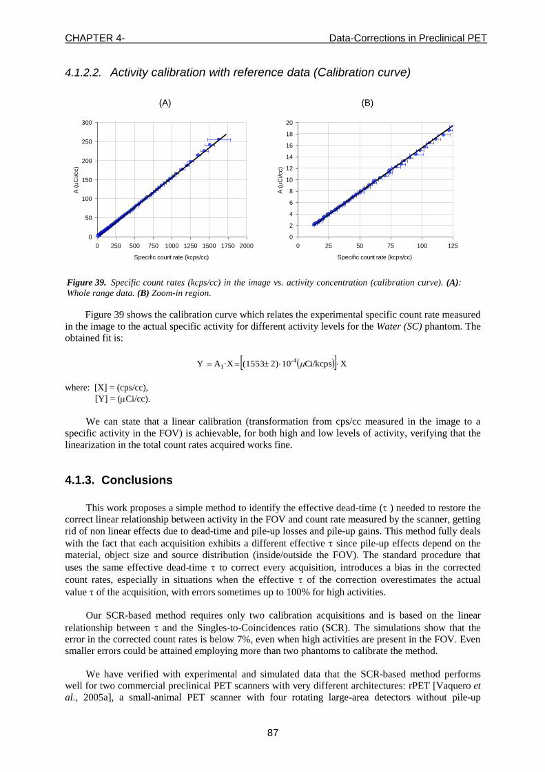
CHAPTER 4- Data-Corrections in Preclinical PET
87
4.1.2.2. Activity calibration with reference data (Calibration curve)
Figure 39 shows the calibration curve which relates the experimental specific count rate measured
in the image to the actual specific activity for different activity levels for the Water (SC) phantom. The
obtained fit is:
X Ci/kcps102) (1553 ·XA Y -41
where: [X] = (cps/cc),
[Y] = (Ci/cc).
We can state that a linear calibration (transformation from cps/cc measured in the image to a
specific activity in the FOV) is achievable, for both high and low levels of activity, verifying that the
linearization in the total count rates acquired works fine.
4.1.3. Conclusions
This work proposes a simple method to identify the effective dead-time ( ) needed to restore the
correct linear relationship between activity in the FOV and count rate measured by the scanner, getting
rid of non linear effects due to dead-time and pile-up losses and pile-up gains. This method fully deals
with the fact that each acquisition exhibits a different effective since pile-up effects depend on the
material, object size and source distribution (inside/outside the FOV). The standard procedure that
uses the same effective dead-time to correct every acquisition, introduces a bias in the corrected
count rates, especially in situations when the effective of the correction overestimates the actual
value of the acquisition, with errors sometimes up to 100% for high activities.
Our SCR-based method requires only two calibration acquisitions and is based on the linear
relationship between and the Singles-to-Coincidences ratio (SCR). The simulations show that the
error in the corrected count rates is below 7%, even when high activities are present in the FOV. Even
smaller errors could be attained employing more than two phantoms to calibrate the method.
We have verified with experimental and simulated data that the SCR-based method performs
well for two commercial preclinical PET scanners with very different architectures: rPET [Vaquero et
al., 2005a], a small-animal PET scanner with four rotating large-area detectors without pile-up
(A) (B)
0
50
100
150
200
250
300
0 250 500 750 1000 1250 1500 1750 2000
Specific count rate (kcps/cc)
A (
uC
i/cc)
0
2
4
6
8
10
12
14
16
18
20
0 25 50 75 100 125
Specific count rate (kcps/cc)
A (
uC
i/cc)
Figure 39. Specific count rates (kcps/cc) in the image vs. activity concentration (calibration curve). (A):
Whole range data. (B) Zoom-in region.

CHAPTER 4- Data-Corrections in Preclinical PET
88
rejection in the electronics, for which pile-up is relatively important, and the Argus scanner [Wang et
al., 2006b], a small-animal PET with more conventional geometry (two full rings) and small-area
detectors. The SCR-based method might be applied to any other scanner, including clinical scanners,
with higher interest in scanners with large detector blocks, as for instance clinical dedicated-breast
PET scanners (or PEM cameras) [Wang et al., 2006a, Wu et al., 2009] or high sensitivity preclinical
PET scanners with close-up detectors [Seidel et al., 2010, Zhang et al., 2011].
4.1.4. Appendix 4.1A. Linear relationship between and SCR
In the limit of low rates, the fraction of coincidences that are free of pile-up and dead-time, fc, can
be written as [Knoll, 2000]:
n1fc (51)
where n is the incident coincidences rate and the effective dead-time for coincidences. Quite
generally in any scanner we can consider a dead-time component (possibly including pile-up effects)
which affects every single event recorded by the scanner. This would be characterized by the ‘singles’
dead-time S. Further, there may be additional dead-time contributions coming from the further
processing of events identified as being part of a coincidence event. This would be an ‘only-
coincidences’ dead-time C. For instance, in a scanner working in singles mode, for which every single
event detected is converted, processed and stored in disk, c would be negligible and the effective
dead-time seen in the recorded coincidences would be just due to the loss of single events. On the
other extreme, there may be scanners working in ‘coincidence only’ mode, which would convert and
store just the events that are identified as being part of a valid coincidence event. In the limit of low
rates, the fraction of coincidences which remains free from dead-time (and pile-up) is related to the
fraction of singles free of dead-time (and pile-up), 1- ns s, as follows:
)1·()1(1 2
Cssc nnnf (52)
where ns is the incident singles rate. This equation just indicates that, in order to record a coincidence,
both single events belonging to it must survive to singles dead-time effects and, further, the resulting
coincidence must survive any coincidence-only dead-time effects. If we work out Eq. (52) to find the
value of , we get in the limit of low count rates (disregarding the terms of second and higher order in
C and s):
Cs
sn
n 2 (53)
We define the Singles-to-Coincidences (SCR) ratio for the incident rates (n) as SCR=ns/n so that Eq.
(53) reads:
Cs SCR 2 (54)
Eq. (54) has been derived here in the limit of low count rates (nss<<1 and nC<<1) and in this
limit it is valid for both the paralyzable and non-paralyzable models. It is straightforward to show that
it is also exactly valid (that is, for any rate) in the case of paralyzable dead-time systems, being the
deviations from (54) relatively small (of logarithmic order) for the case of non-paralyzable dead-time
systems.

CHAPTER 4- Data-Corrections in Preclinical PET
89
Eq. (54) shows that under rather general grounds, a linear relationship between the effective dead-
time seen in the acquired coincidences and SCR emerges. It also shows that the slope and intercept of
a linear fit of the effective against SCR will estimate the effective singles dead-time, which may
include pile-up effects, and the coincidences-only dead-time, respectively.
4.1.5. Appendix 4.1B. Relative error in the corrected count rates as a function of the error in the effective dead-time
Let n be the count rates corrected by the true value of the effective dead-time, , for one
acquisition and n’ the count rates corrected by the estimated effective dead-time, ( +), being the
error in the effective dead-time. We can write:
m
mn
1 and
m
mn
1' (55)
where these two count rates are related by:
n
nn
1' (56)
So the relative error of the corrected count rates is:
n
n
n
nnEr
1
' (57)
Equation (57) shows that the relative error increases much faster with n when is overestimated
( > 0) than when it is underestimated ( < 0).

CHAPTER 4- Data-Corrections in Preclinical PET
90
4.2. Measurement of misalignments in small-animal PET scanners based on rotating planar detectors and parallel-beam geometry
The increasing number of animal models of human diseases used in translational research makes
small-animal imaging an essential tool to assess biological functions. This approach makes it possible
to carry out new types of studies, such as monitoring of transgenic expression in genetically modified
mice or in vivo monitoring of tumor response to therapy [Lewis and Achilefu, 2002, Pomper, 2001,
Massoud and Gambhir, 2003]. In these systems, the dimensions of the structures whose biochemical
functions we want to analyze impose additional system requirements not shared by clinical scanners
[Lecomte, 2004]. To address the same biological questions that are already being investigated in
humans, both systems must provide similar relation between spatial resolution and size of the organ
under study, which is know as ‘image equivalence’ [Jagoda et al., 2004]. This suggests that a small-
animal system would have to reconstruct images with a resolution below 1 mm in all directions,
whereas systems for imaging human tissue typically have a resolution of ~4-10 mm. Therefore, exact
geometric characterization is critical in small-animal scanners, as even submillimetric misalignments
of the detectors may result in noticeable degraded image resolution and artifacts. Figure 40 illustrates
this effect with a rat study affected by a detector misalignment in the range of half the crystal pitch
size (one detector was misplaced by 0.8 mm). Acquired data were reconstructed with FBP with a
sinogram bow-tie filtering scheme [Abella et al., 2009].
Figure 40. Coronal, sagittal, and axial views of an FDG rat study acquired with the rPET scanner and
reconstructed with FBP with a bow-tie filtering scheme. Reconstructed volume was 55x55x55 with isotropic 0.8
mm pixel size. Result before (top) and after (bottom) correcting for misalignments in the range of half the crystal
pitch size (one detector was misplaced by 0.8 mm).
Methods for estimating geometrical parameters of tomography scanners have been investigated
since 1987, mainly for CT and SPECT systems based on fan-beam geometry [Hsieh, 1992, Gullberg et
al., 1987] and cone-beam geometry [Gullberg et al., 1990, Noo et al., 2000, Beque et al., 2003, Sun et
al., 2007]. Systems based on parallel-beam geometry have received little attention. In [Azevedo et al.,
1990] the authors studied methods for estimating the center of rotation (COR) in CT using sinogram
data; [Busemann-Sokole, 1987] proposed a method for the determination of collimator hole
angulations in SPECT scanners, and, more recently, [Donath et al., 2006] presented an iterative
procedure for the determination of the position of the optimum COR intended for any tomography
system. Few contributions have been made on the specific case of rotating PET systems, except for a

CHAPTER 4- Data-Corrections in Preclinical PET
91
preliminary study of the effect of misalignments by our group [Abella et al., 2006]. More recently,
Pierce et al. proposed a new calibration method to determine block positions in a system based on a
ring of PET detectors [Pierce et al., 2009]. To the best of our knowledge, there are no systematic
studies of the effect of all possible misalignments in a tomography system based on rotating planar
detectors.
Calibration techniques are usually based on analytical expressions applicable to the acquisition of
ad-hoc phantoms, which sometimes require precise positioning in the field of view (FOV). In our
experience, these analytic algorithms should only be used to provide an initial appraisal of
misalignment parameters, as most of them make assumptions of ideal or negligible conditions that
may not hold in real scanners, and usually require further fine tuning.
We analyzed misalignment effects in PET systems based on rotating detectors with parallel-beam
geometry and defined a robust and easy-to-implement protocol for geometric characterization [Abella
et al., 2012]. The result of the calibration step can then be used to generate the correct 3D-sinogram
from the acquired list-mode data. Section 4.2.1 presents a description of the simulations used. Section
4.2.2 describes the misalignments considered in this work and provides a theoretical study of the
effects of these misalignments on projection data and of the tolerance of the system to each one, in
order to define an easy way for detection and calibration. Section 4.2.3 proposes the algorithm to
measure these misalignments in a real scanner. Finally, section 4.2.4 presents an evaluation of the
calibration tool proposed.
4.2.1. Monte Carlo simulations using PeneloPET
In order to study and quantify the effects of the different geometrical misalignments and to
evaluate the proposed algorithm, we used the simulation package PeneloPET (see chapter 2, section
2.3). In the simulations, detector blocks can be displaced from their regular positions in order to build
non-regular complex geometries or to introduce misalignments of detectors [España et al., 2009].
Simulations were done based on the high-resolution animal rPET scanner (see chapter 2, section
2.1). In this system, 3D data approximate line integrals of the radioactive tracer distribution along
lines of response (LOR) that are not restricted to transaxial planes. Data measured by each detector
pair are rearranged into a set of direct 2D sinograms, which only include LORs from transaxial slices,
and oblique 2D sinograms, which traverse several slices, thus conforming a 3D sinogram as a function
of three variables (ρ, θ, s). ρ is the distance between the LOR and the COR (ranging from 0 to R
(radius of the FOV)), θ is the azimuthal angle between the LOR and the Y0-axis (ranging from 0 to
180 degrees (Figure 41, left), and s is an integer variable which accounts for the different 2D
sinograms (ranging from 0 to 282). These sinograms cover all the possible combinations formed by the
events registered by detector elements on different rows.
Data for angles over 360 degrees are reallocated at the corresponding 2D sinogram position in the
range 0-180 degrees, as derived from the symmetry property
),(),( pp (58)
where ),( p is the data measured in an LOR defined by the pair ),( for a given s. As a result,
there is a region where the extra 14 degrees from the first and last position of the detectors overlap
(Figure 41, right). Each 2D sinogram has 55 radial and 120 angular bins, resulting in a spacing of 0.8
mm and 1.5 degrees in the radial and angular directions, respectively.

CHAPTER 4- Data-Corrections in Preclinical PET
92
Figure 41. Left: Transaxial view showing the 2D sinogram variables ρ and θ used to parameterize the LORs.
Right: Rearrangement of the data, from a 360-degree 2D sinogram into a 180-degree 2D sinogram.
Two point source studies with different misalignment configurations were simulated: one located
at the center of the FOV and the other one at 10 mm from the center of the FOV, both in the central
axial slice. The point source consisted of a sphere (0.5 mm of diameter) of 18
F of 30 uCi in a cubic
phantom (111 cm3) of water. We chose an acquisition time of 320 s, which provided a total number
of acquired coincidences of around 7·106 (center) and 6·10
6 (1 cm off-center).
Finally, a Hot Derenzo Phantom (see Appendix A) acquisition was simulated with and without
misalignments to evaluate the effect of the remaining misalignments within the tolerance of the
presented method on the corrected image quality. The initial activity was 11.2 MBq (300 μCi) and the
acquisition time 560 s (total number of acquired coincidences: 3·107). The misalignments used in this
simulation are listed below:
x1 = 0.0, x2 = 5.0, x3 = 2.5, x4 = -2.5,
y1 = 0.0, y2 = 1.6, y3 = 0.8, y4 = -0.8,
z1 = 0.0, z2 = 0.0, z3 = 0.0, z4 = 0.0,
Фoffset = 88.0
4.2.2. Study of the effect of misalignments
Figure 42. Left: Detector attached to the rotating gantry showing the three possible sources of angular errors
in the detector position in relation to the gantry: σ, , and . Right: Axial view of the system showing the
coordinate systems used: X0, Y0, and Z0 are absolute coordinates and (x1,y1,z1) and (x2,y2,z2) are coordinates
relative to detectors 1 and 2, respectively.
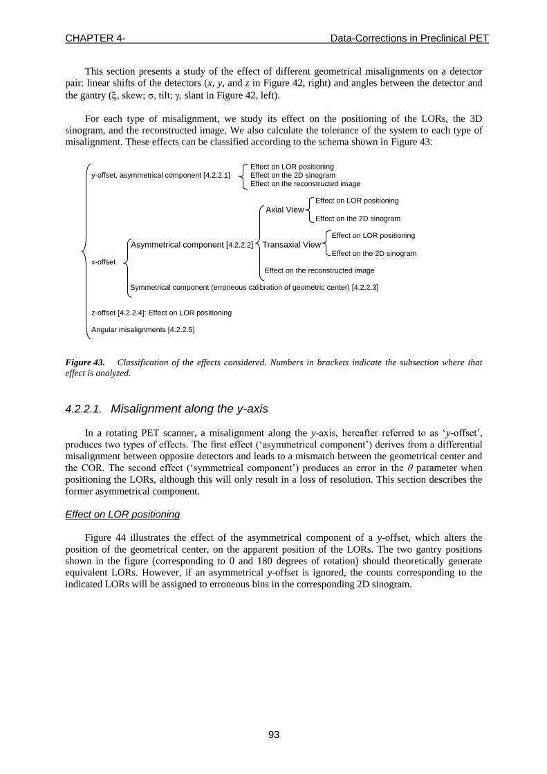
CHAPTER 4- Data-Corrections in Preclinical PET
93
This section presents a study of the effect of different geometrical misalignments on a detector
pair: linear shifts of the detectors (x, y, and z in Figure 42, right) and angles between the detector and
the gantry (, skew; σ, tilt; slant in Figure 42, left).
For each type of misalignment, we study its effect on the positioning of the LORs, the 3D
sinogram, and the reconstructed image. We also calculate the tolerance of the system to each type of
misalignment. These effects can be classified according to the schema shown in Figure 43:
Figure 43. Classification of the effects considered. Numbers in brackets indicate the subsection where that
effect is analyzed.
4.2.2.1. Misalignment along the y-axis
In a rotating PET scanner, a misalignment along the y-axis, hereafter referred to as ‘y-offset’,
produces two types of effects. The first effect (‘asymmetrical component’) derives from a differential
misalignment between opposite detectors and leads to a mismatch between the geometrical center and
the COR. The second effect (‘symmetrical component’) produces an error in the θ parameter when
positioning the LORs, although this will only result in a loss of resolution. This section describes the
former asymmetrical component.
Effect on LOR positioning
Figure 44 illustrates the effect of the asymmetrical component of a y-offset, which alters the
position of the geometrical center, on the apparent position of the LORs. The two gantry positions
shown in the figure (corresponding to 0 and 180 degrees of rotation) should theoretically generate
equivalent LORs. However, if an asymmetrical y-offset is ignored, the counts corresponding to the
indicated LORs will be assigned to erroneous bins in the corresponding 2D sinogram.
Effect on LOR positioning y-offset, asymmetrical component [4.2.2.1] Effect on the 2D sinogram Effect on the reconstructed image
Effect on LOR positioning
Axial View Effect on the 2D sinogram
Effect on LOR positioning
Asymmetrical component [4.2.2.2] Transaxial View Effect on the 2D sinogram
x-offset Effect on the reconstructed image
Symmetrical component (erroneous calibration of geometric center) [4.2.2.3]
z-offset [4.2.2.4]: Effect on LOR positioning Angular misalignments [4.2.2.5]

CHAPTER 4- Data-Corrections in Preclinical PET
94
Figure 44. Drawing of a detector pair in two gantry positions that should theoretically generate coincident
LORs. The star represents an annihilation event. Detector 1 has a y-offset of y1 = -3.2 mm (two-crystal
widths). The panels labeled (a) show the LOR in the real position of the detectors, while the panels labeled (b)
show the apparent LOR that would be obtained if the offset were ignored. Panel (c) shows the shift
quantification. 1 is the radial coordinate in the 2D sinogram corresponding to the apparent LOR when the
detectors are at 0 degrees and 2 corresponds to the apparent LOR with the detectors at 180 degrees.
Effect on the 2D sinogram
Figure 45 shows the consequence of this type of LOR positioning error on the 180-degree 2D
sinogram in our experimental setup: the region of overlap (zoomed-in view in Figure 45 (a)) shows a
discontinuity that we refer to as ‘radial gap’ in the bins corresponding to gantry positions with 180
degrees of difference. This gap is only visible in the 14-degree sector, which is scanned twice in one
rotation, as explained above. Data at the left side of the radial gap (1 in Figure 45 (a)) correspond to
events read while the detectors were at the 0-degree gantry position, and data to the right of the radial
gap (2 in Figure 45 (a)) were acquired with the detectors at 180 degrees. The y-offset, Δy, is directly
related to the number of radial bins, n, in the sinogram spanned by the discontinuity, according to:
nby (59)
where b is the radial bin size in mm and y is the y-offset. Due to the binning in the sinogram, n is an
integer value, and it can be seen from equation Figure 45 that the estimate for y will be discredited
(size of the radial bin, b). The value n only depends on the amount of mismatch between the geometric
center and the COR, which is a function of the relative displacement between detectors. The ‘sign’ of
the radial gap is related to the direction of the mismatch between the geometric center and the COR.

CHAPTER 4- Data-Corrections in Preclinical PET
95
Figure 45. Example of a y-offset with an asymmetrical component (mismatch between the geometrical center
and the COR). (a) Zoomed-in view of the overlap region, showing the radial gap. Labels 1 and 2 identify data
acquired at positions 1 (detectors at 0 degrees) and 2 (detectors at 180 degrees) in Figure 44. (b) Radial profile
across the gap region.
Effect on the reconstructed image
Figure 46 shows the effect of a mismatch between the COR and the geometric center on the
reconstructed image of a point source, which is a ‘crescent’ shape of the image that deteriorates
resolution. The simulation corresponds to a point source located at 10 mm from the center of the FOV
in the central slice.
Figure 46. Effect of a y-offset on the reconstructed image resolution. Left: transaxial view of a simulated point
source for a y-offset of 1.6 mm showing a ‘crescent’ shape. Right: FWHM of profiles drawn along the Yo-axis for
different values of the y-offset.
A summary of the effects and tolerance for the y-offset is presented in Table 25 (rows 1 and 2).
4.2.2.2. Misalignment along the x-axis with mismatch between geometric center and COR
The misalignment along the x-axis, hereafter referred to as ‘x-offset’, may also lead to two types
of effect. The first one derives from a differential misalignment between opposite detectors and leads
to a mismatch between the geometrical center and the COR (‘asymmetrical component’). The second
one occurs when both detectors are misplaced the same amount in opposite directions and leads to
erroneous calibration of the distance between detectors (see section 4.2.2.3). This section describes the
asymmetrical component.
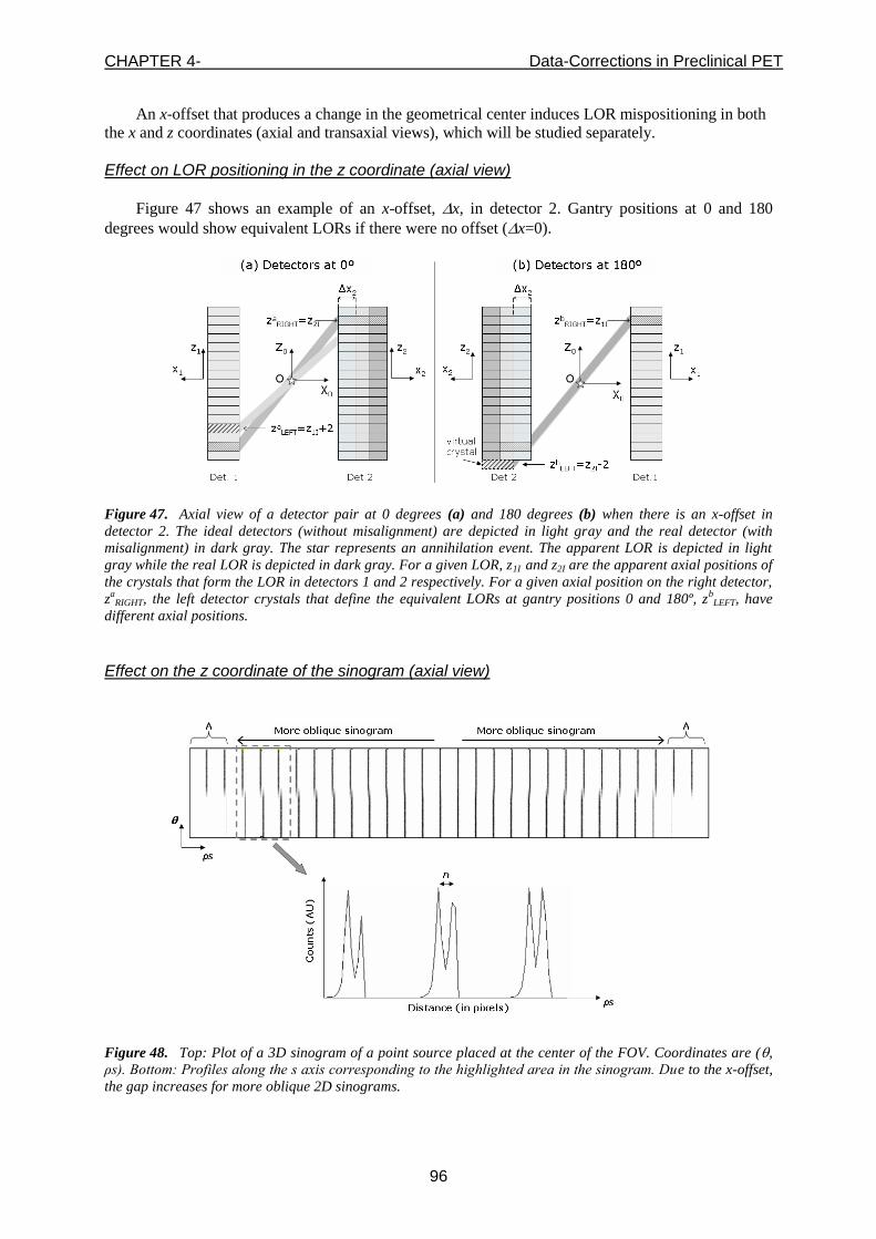
CHAPTER 4- Data-Corrections in Preclinical PET
96
An x-offset that produces a change in the geometrical center induces LOR mispositioning in both
the x and z coordinates (axial and transaxial views), which will be studied separately.
Effect on LOR positioning in the z coordinate (axial view)
Figure 47 shows an example of an x-offset, x, in detector 2. Gantry positions at 0 and 180
degrees would show equivalent LORs if there were no offset (x=0).
Figure 47. Axial view of a detector pair at 0 degrees (a) and 180 degrees (b) when there is an x-offset in
detector 2. The ideal detectors (without misalignment) are depicted in light gray and the real detector (with
misalignment) in dark gray. The star represents an annihilation event. The apparent LOR is depicted in light
gray while the real LOR is depicted in dark gray. For a given LOR, z1I and z2I are the apparent axial positions of
the crystals that form the LOR in detectors 1 and 2 respectively. For a given axial position on the right detector,
za
RIGHT, the left detector crystals that define the equivalent LORs at gantry positions 0 and 180º, zbLEFT, have
different axial positions.
Effect on the z coordinate of the sinogram (axial view)
Figure 48. Top: Plot of a 3D sinogram of a point source placed at the center of the FOV. Coordinates are (,
ρs). Bottom: Profiles along the s axis corresponding to the highlighted area in the sinogram. Due to the x-offset,
the gap increases for more oblique 2D sinograms.

CHAPTER 4- Data-Corrections in Preclinical PET
97
Figure 48 shows a plot of a 3D sinogram for coordinates θ (120 bins) and ρs (55×282 bins). Note
that the most oblique 2D sinograms containing the point source (A in Figure 48) lack half of the
angular positions. This is because that there is no opposite crystal to conform the LOR in those
extreme positions (Figure 47b).
Since the size of these discontinuities in the sinogram is directly related to the x-offset, it is
possible to estimate this offset from the axial gaps measured on the sinograms. Figure 49 shows a
zoomed-in picture of the top half of one detector, depicting the real and apparent detector positions.
Figure 49. Diagram of the top half of one detector showing the rationale for the estimation of the x-offset. In
light gray we have The detector in the ideal position is shown in light gray and the detector in the real position
(with misalignment) is shown in dark gray. R is the radius of rotation, p the pitch size, N the number of crystals
in the axial direction, l the crystal thickness, and Δx the x-offset of the detector.
The value of Δx can be obtained from simple trigonometric relations. For the upper crystal row of
the detector we have:
2
5.02/
2
5.02/
lR
nNp
xlR
Np
(60)
where R is the radius of rotation, N is the number of crystals in the detector along the z-axis, l is the
crystal thickness, p is the pitch size, and n is the number of crystals by which the LOR is misplaced
(equal to half the axial gap in sinogram bins). Thus, the value of Δx can be calculated as
nN
nlRx
5.02
)2/( (61)
This effect will appear in the 3D sinogram if there is a minimum change of one crystal in the
position of the LORs, i. e. n=1. Equation (61) shows that the minimum value for the calculated x-
offset, Δx, to have an effect is about 7 mm.
Knowledge of the position of the detectors along the x-axis enables a software correction that will
lead to correct positioning of the counts in the sinogram. Thus, good quality images can be
reconstructed despite the physical mismatch between the geometrical center and the COR. The gap
size can be used to obtain a rough estimate of the asymmetrical component of an x-offset, as explained
above. In order to refine this estimate we can use the effect on the ‘transaxial view’ (see following
section).

CHAPTER 4- Data-Corrections in Preclinical PET
98
Effect on LOR positioning in the x coordinate (transaxial view)
In the case of an asymmetrical x-offset, the LORs corresponding to the initial and final rotating
positions (gantry at 0 and 180 degrees), which should be equivalent, will show the same θ value but a
different ρ value in the 2D sinogram (Figure 50c).
Figure 50. Axial view of a detector pair at gantry positions corresponding to 0 degrees (a) and 180 degrees
(b). The real detector (with misalignment) is depicted in dark gray while the ideal one is depicted in light gray.
The star represents an annihilation event. For a given crystal position in detector 1, y1A, and a given angle, θ,
the real LOR is depicted in dark gray and the apparent LOR if the x-offset were ignored is depicted in light gray.
In (c), we see that the apparent LORs read at 0 and 180 degrees that should coincide show the same angle but
different ρ value.
Effect on the 3D sinogram in the x coordinate (axial view)
The error in the LOR positioning explained above results in a widening of the 2D sinogram. In
our experimental setup, due to the arrangement in a 180-degree sinogram, the sinogram area
corresponding to the initial and final gantry positions shows a characteristic shape (gray dotted square
in Figure 51, left). The right panel of Figure 51 shows that the trajectory followed by the center of
mass along the ρ-coordinate presents a deviation from the expected profile at the overlap area. The
amount of deviation corresponds to half the differential x-offset of the system. This value also reflects
the difference between the COR and center of the FOV.
Figure 51. Left: Sum of all oblique 2D sinograms for different x-offset values {1, 2, 3 cm}. Right: Center of
mass vector for each 2D sinogram on the left.
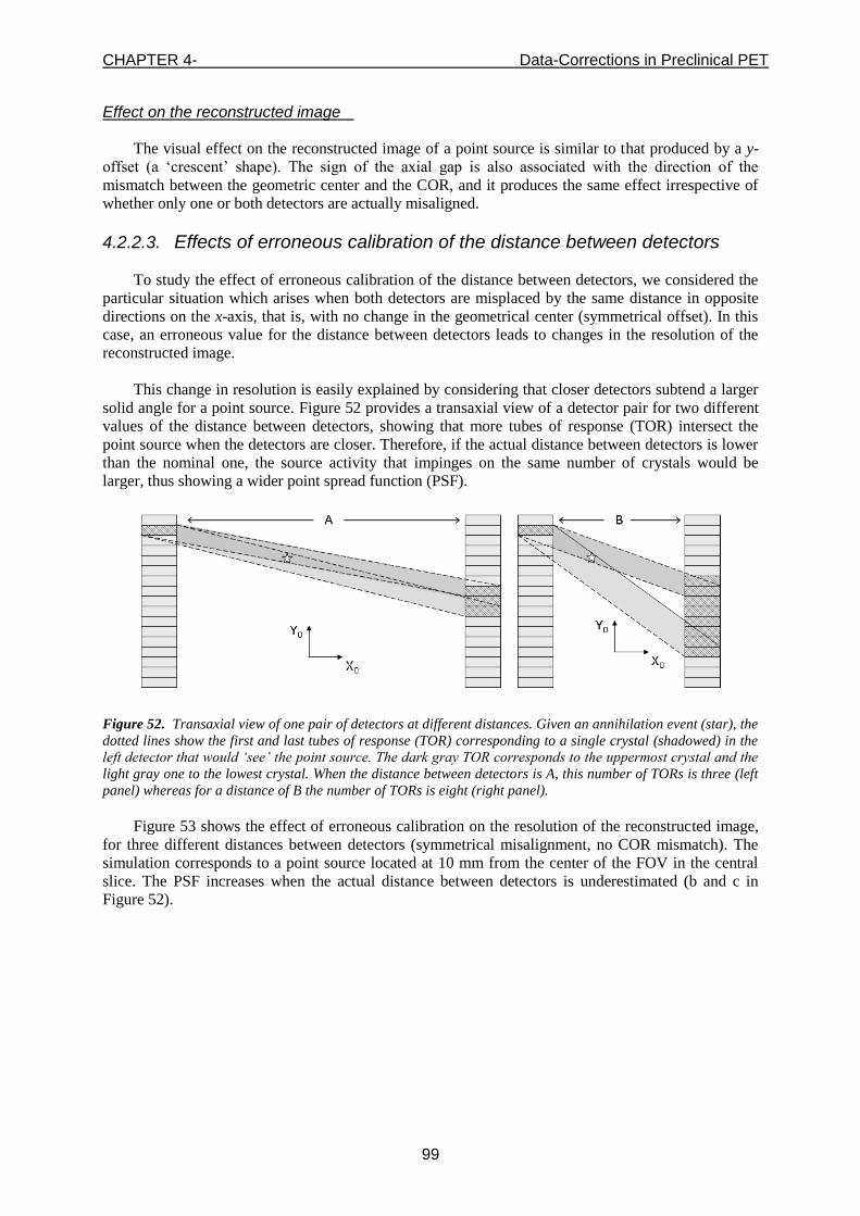
CHAPTER 4- Data-Corrections in Preclinical PET
99
Effect on the reconstructed image
The visual effect on the reconstructed image of a point source is similar to that produced by a y-
offset (a ‘crescent’ shape). The sign of the axial gap is also associated with the direction of the
mismatch between the geometric center and the COR, and it produces the same effect irrespective of
whether only one or both detectors are actually misaligned.
4.2.2.3. Effects of erroneous calibration of the distance between detectors
To study the effect of erroneous calibration of the distance between detectors, we considered the
particular situation which arises when both detectors are misplaced by the same distance in opposite
directions on the x-axis, that is, with no change in the geometrical center (symmetrical offset). In this
case, an erroneous value for the distance between detectors leads to changes in the resolution of the
reconstructed image.
This change in resolution is easily explained by considering that closer detectors subtend a larger
solid angle for a point source. Figure 52 provides a transaxial view of a detector pair for two different
values of the distance between detectors, showing that more tubes of response (TOR) intersect the
point source when the detectors are closer. Therefore, if the actual distance between detectors is lower
than the nominal one, the source activity that impinges on the same number of crystals would be
larger, thus showing a wider point spread function (PSF).
Figure 52. Transaxial view of one pair of detectors at different distances. Given an annihilation event (star), the
dotted lines show the first and last tubes of response (TOR) corresponding to a single crystal (shadowed) in the
left detector that would ‘see’ the point source. The dark gray TOR corresponds to the uppermost crystal and the
light gray one to the lowest crystal. When the distance between detectors is A, this number of TORs is three (left
panel) whereas for a distance of B the number of TORs is eight (right panel).
Figure 53 shows the effect of erroneous calibration on the resolution of the reconstructed image,
for three different distances between detectors (symmetrical misalignment, no COR mismatch). The
simulation corresponds to a point source located at 10 mm from the center of the FOV in the central
slice. The PSF increases when the actual distance between detectors is underestimated (b and c in
Figure 52).
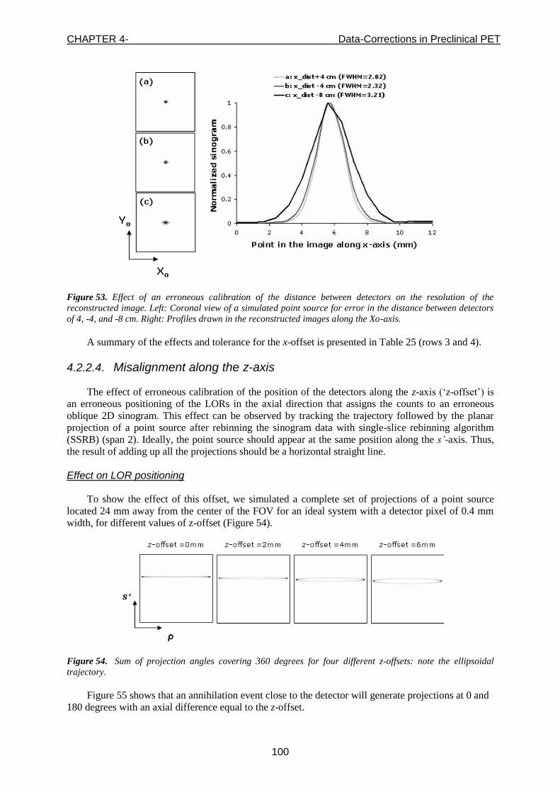
CHAPTER 4- Data-Corrections in Preclinical PET
100
Figure 53. Effect of an erroneous calibration of the distance between detectors on the resolution of the
reconstructed image. Left: Coronal view of a simulated point source for error in the distance between detectors
of 4, -4, and -8 cm. Right: Profiles drawn in the reconstructed images along the Xo-axis.
A summary of the effects and tolerance for the x-offset is presented in Table 25 (rows 3 and 4).
4.2.2.4. Misalignment along the z-axis
The effect of erroneous calibration of the position of the detectors along the z-axis (‘z-offset’) is
an erroneous positioning of the LORs in the axial direction that assigns the counts to an erroneous
oblique 2D sinogram. This effect can be observed by tracking the trajectory followed by the planar
projection of a point source after rebinning the sinogram data with single-slice rebinning algorithm
(SSRB) (span 2). Ideally, the point source should appear at the same position along the s’-axis. Thus,
the result of adding up all the projections should be a horizontal straight line.
Effect on LOR positioning
To show the effect of this offset, we simulated a complete set of projections of a point source
located 24 mm away from the center of the FOV for an ideal system with a detector pixel of 0.4 mm
width, for different values of z-offset (Figure 54).
Figure 54. Sum of projection angles covering 360 degrees for four different z-offsets: note the ellipsoidal
trajectory.
Figure 55 shows that an annihilation event close to the detector will generate projections at 0 and
180 degrees with an axial difference equal to the z-offset.

CHAPTER 4- Data-Corrections in Preclinical PET
101
Figure 55. Axial view of a detector pair at 0 degrees (a) and 180 degrees (b) when there is a z-offset of Δz1 in
detector 1. The star represents an annihilation event. When the gantry is at the starting position (a), the ‘direct’
LOR that contains the event is different from the one at 180 degrees. For this reason, projection at different
angles will show the point source at different axial positions.
For annihilation events originated at a distance R from the axis of rotation, we can derive a
formula to estimate the z-offset, by applying simple trigonometric relations, as follows:
RDBD
axialdiffDBDoffsetz
RDBD
axialdiff
DBD
offsetz
22
(62)
where DBD is the distance between detectors, R is the distance to the COR, and axialdiff is the length
of the short axis of the ellipsoidal trajectory.
Since the achievable resolution in the projections with the scanner under study is only about 0.8
mm, the ellipsoidal shape of the trajectory is barely visible. Thus, the effect of a z-offset in practice
will appear as an increase in the FWHM of the profile along the z-axis. This increase will only be
visible when there is a change in the axial positions of the LORs that requires a z-offset higher than the
crystal pitch. A summary of the effects and tolerance for the z-offset is presented in Table 25 (row 5).
4.2.2.5. Angular misalignments
As shown in the left panel of Figure 42, the detector may have angular misalignments around the
three axes, Xo, Yo, Zo.
Effect of slant and tilt
Both slant and tilt, (angular rotations around Yo and around Zo), produce the same effect in a
system with planar detectors. From Figure 56 we can see that the minimum value of σ that would
generate a noticeable effect, i.e. that would change the identification of the crystals involved in the
LOR, is given by the equation:
2/)tan( min
l
pitch (63)
where pitch is the distance between the center of two adjacent crystals and l is the crystal length.
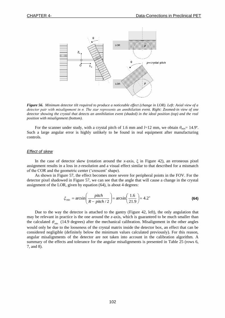
CHAPTER 4- Data-Corrections in Preclinical PET
102
Figure 56. Minimum detector tilt required to produce a noticeable effect (change in LOR). Left: Axial view of a
detector pair with misalignment in σ. The star represents an annihilation event. Right: Zoomed-in view of one
detector showing the crystal that detects an annihilation event (shaded) in the ideal position (top) and the real
position with misalignment (bottom).
For the scanner under study, with a crystal pitch of 1.6 mm and l=12 mm, we obtain θmin= 14.9º.
Such a large angular error is highly unlikely to be found in real equipment after manufacturing
controls.
Effect of skew
In the case of detector skew (rotation around the x-axis, ξ in Figure 42), an erroneous pixel
assignment results in a loss in z-resolution and a visual effect similar to that described for a mismatch
of the COR and the geometric center (‘crescent’ shape).
As shown in Figure 57, the effect becomes more severe for peripheral points in the FOV. For the
detector pixel shadowed in Figure 57, we can see that the angle that will cause a change in the crystal
assignment of the LOR, given by equation (64), is about 4 degrees:
o
min 2.49.21
6.1arcsin
2/arcsin
pitchR
pitch (64)
Due to the way the detector is attached to the gantry (Figure 42, left), the only angulation that
may be relevant in practice is the one around the z-axis, which is guaranteed to be much smaller than
the calculated min (14.9 degrees) after the mechanical calibration. Misalignment in the other angles
would only be due to the looseness of the crystal matrix inside the detector box, an effect that can be
considered negligible (definitely below the minimum values calculated previously). For this reason,
angular misalignments of the detector are not taken into account in the calibration algorithm. A
summary of the effects and tolerance for the angular misalignments is presented in Table 25 (rows 6,
7, and 8).

CHAPTER 4- Data-Corrections in Preclinical PET
103
Figure 57. Rotation of one detector around the x-coordinate.
4.2.2.6. Summary
Table 25 summarizes our results, indicating the formula for the minimum value necessary to
produce a visible effect (what we call ‘tolerance’) and the value for the particular case of the rPET
system studied.
Table 25. Summary of the study of misalignments. For each misalignment type the table indicates the simulation
study used to assess its effect on the sinogram and on the reconstructed image, the tolerance formula (minimum
value to produce a noticeable effect) and its value for the particular case of the rPET system.
Misalignment Acquisition Effect on sinogram
Effect on image Tolerance Value for the rPET system
y-offset, affecting COR (asymmetrical)
Non-centered
point source Radial gap Crescent shape Half pitch size 0.8 mm
y-offset, not affecting COR (symmetrical)
Non-centered
point source
Higher FWHM in coronal view
Transaxial resolution loss
Not considered Not
considered
x-offset, affecting COR (asymmetrical)
Centered-FOV point
source
Axial gap Center of mass
modified Higher FWHM in
coronal view
Crescent shape
5.12
1
2 NlRx
7 mm
x-offset, not affecting COR (symmetrical)
Non-centered
point source
Higher FWHM in coronal view
Axial and transaxial
resolution loss Not considered
Not considered
z-offset Any point
source Higher FWHM in
sagittal view Axial resolution
loss Pitch size 1.6 mm
Tilt (along y-axis) Non
centered point source
Radial gap Axial resolution
loss )2/(arctanmin
l
pitch
14.9º
Slant (along z-axis) Any known
point source location
Higher FWHM in sagittal view
Crescent shape )2/(
arctanminl
pitch 14.9º
Skew
Non-centered
point source (both in x-y
and z)
Radial gap and higher FWHM in
axial view
Transaxial and axial resolution
loss
2/arcsinmin
pitchR
pitch
4.2º
All the misalignments in Table 25 correspond to a single pair of detectors. In a system with more
than one pair of detectors, such as the one under study here, there are two additional calibration

CHAPTER 4- Data-Corrections in Preclinical PET
104
parameters to measure: the z-offset between detector pairs and the angle between detector pairs (angle
Фoffset in Figure 42, right). We did not perform any simulation of these two misalignments, since the
procedure to obtain their values is straightforward (explained below).
4.2.3. Calibration algorithm
The results of the presented study enabled us to develop a calibration algorithm to calculate
scanner misalignments. The input data for the algorithm are two acquisitions in coincidence list-mode
of a small spherical 22
Na point source (in our case, 0.3 mm in diameter, encapsulated in a 1-cm3 epoxy
box. In the first acquisition, the source is placed at the center of the FOV (‘centered acquisition’) and
in the second one the source is located 11 mm away from that center in the transaxial plane (‘non-
centered acquisition’). Intermediate reconstructions are generated by means of SSRB with span 1,
followed by a 2D filtered back-projection (FBP) with a ramp filter. For the rPET scanner, the voxel
size of the resulting image is 0.8 mm isotropic. The result of the calibration algorithm is a file
containing the misalignment values. This file is used by subsequent reconstructions to generate a
corrected sinogram, in which the position of each LOR is relocated according to the actual
misalignments. Figure 58 shows a flowchart of the calibration process and the interface of the
calibration tool at the end of the process.
Figure 58. Flowchart of the calibration algorithm. Dotted lines indicate iterative paths for a fine tuning of
the offset values.Left: Interface of the calibration tool at the end of the process showing the sinogram from
each pair of detector and the summed sinogram, the misalignment values found, and the resulting resolution.
For each offset, the program makes a first estimate and guides the user through an interactive
tuning procedure. After an initial estimation of all the offsets, in a process called coarse tuning, the
software offers the user the possibility of performing more iterations of the calibration algorithm using
smaller offset values (fine tuning) until the result is satisfactory. When this process has finished for all
the possible offsets, the final values are stored.
The following subsections present a detailed explanation of the processing performed at each step
of the flow chart.
4.2.3.1. Estimation of z-offset
For the measurement of the z-offset between the two detectors of a pair, the calibration protocol
makes use of the centered acquisition and generates sinograms for different values of the detector 1
position along the z-axis, z’1, as follows:
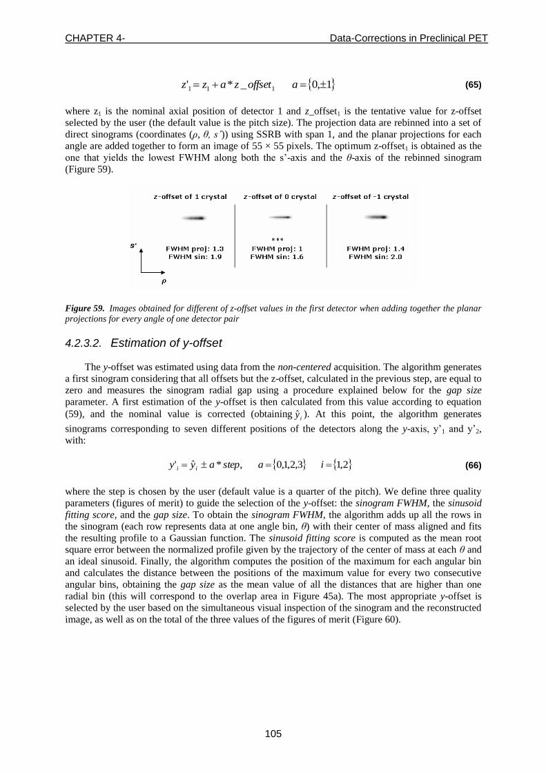
CHAPTER 4- Data-Corrections in Preclinical PET
105
1,0_*' 111 aoffsetzazz (65)
where z1 is the nominal axial position of detector 1 and z_offset1 is the tentative value for z-offset
selected by the user (the default value is the pitch size). The projection data are rebinned into a set of
direct sinograms (coordinates (ρ, θ, s’)) using SSRB with span 1, and the planar projections for each
angle are added together to form an image of 55 × 55 pixels. The optimum z-offset1 is obtained as the
one that yields the lowest FWHM along both the s’-axis and the θ-axis of the rebinned sinogram
(Figure 59).
Figure 59. Images obtained for different of z-offset values in the first detector when adding together the planar
projections for every angle of one detector pair
4.2.3.2. Estimation of y-offset
The y-offset was estimated using data from the non-centered acquisition. The algorithm generates
a first sinogram considering that all offsets but the z-offset, calculated in the previous step, are equal to
zero and measures the sinogram radial gap using a procedure explained below for the gap size
parameter. A first estimation of the y-offset is then calculated from this value according to equation
(59), and the nominal value is corrected (obtainingiy ). At this point, the algorithm generates
sinograms corresponding to seven different positions of the detectors along the y-axis, y’1 and y’2,
with:
2,13,2,1,0,*ˆ' iastepayy ii (66)
where the step is chosen by the user (default value is a quarter of the pitch). We define three quality
parameters (figures of merit) to guide the selection of the y-offset: the sinogram FWHM, the sinusoid
fitting score, and the gap size. To obtain the sinogram FWHM, the algorithm adds up all the rows in
the sinogram (each row represents data at one angle bin, θ) with their center of mass aligned and fits
the resulting profile to a Gaussian function. The sinusoid fitting score is computed as the mean root
square error between the normalized profile given by the trajectory of the center of mass at each θ and
an ideal sinusoid. Finally, the algorithm computes the position of the maximum for each angular bin
and calculates the distance between the positions of the maximum value for every two consecutive
angular bins, obtaining the gap size as the mean value of all the distances that are higher than one
radial bin (this will correspond to the overlap area in Figure 45a). The most appropriate y-offset is
selected by the user based on the simultaneous visual inspection of the sinogram and the reconstructed
image, as well as on the total of the three values of the figures of merit (Figure 60).

CHAPTER 4- Data-Corrections in Preclinical PET
106
Figure 60. Estimation of the y-offset. Example of calculated values for ‘gap size’, ‘sinogram FWHM’, and
‘sinusoid fitting score’ (left), reconstructed image (middle), and sinograms (right) for different values of y-offset.
4.2.3.3. Estimation of x-offset
The calibration protocol estimates the x-offset using the centered acquisition data. The algorithm
generates a sinogram corrected for the offsets already estimated (z- and y-offset) and provides an
initial estimation of the x-offset according to equation (61) and the axial gap size in the sinogram.
The algorithm then generates sinograms corresponding to seven different positions of detector 1
along the x-axis, x’1, assuming that position of detector 2 along the x-axis is correct (thus, ignoring the
symmetrical component), as follows:
2,13,2,1,0,*ˆ' 11 iastepaxx (67)
where
1x is the ideal value corrected with the initial estimate of x-offset and the step is chosen by the
user (default value is 2 mm).
For each sinogram, the algorithm calculates two figures of merit: the sinogram FWHM, explained
above, and the deviation of the center of mass shown in Figure 51, right. The selection of the
appropriate x-offset is made by the user based on the visual inspection of the sinogram, the
reconstructed image, and the figures of merit defined, for each tested value.
4.2.3.4. Estimation of z-offset between detector pairs
Once each pair of detectors is corrected for x- and y-offsets, the calibration algorithm determines
the z-offset between detector pairs. For each detector pair, the algorithm generates an image by adding
up the planar projections for every angle. The z-offset between detector pairs is calculated as the
difference between the center of mass along the z-axis for each image, as shown in Figure 61.

CHAPTER 4- Data-Corrections in Preclinical PET
107
Figure 61. Images obtained by adding-up the planar projection for every angle of the two detector pairs, for
different values of z-offset between detectors.
4.2.3.5. Estimation of the angle between blocks
The last step is to determine the angle between detector pairs, which theoretically is 90 degrees
(angle Фoffset in Figure 42, right). To this end, the algorithm compares the trajectory drawn by the
center of mass for every angle bin (θ dimension) of one detector pair with that obtained from other
detector pair with different shift values, θshift. The shift value that leads to the least error (first column
in Figure 62), two coincident trajectories (second column in Figure 62), and two coincident sinograms
(third column in Figure 62) is selected as the Фoffset.
Figure 62. Center of mass trajectory for each detector pair and difference image of both sinograms. The
central row shows the optimum value.
4.2.4. Evaluation
As mentioned above, the method proposed only detects absolute misalignments, without
discriminating if it was produced by one or both detectors within the pair. We estimated the effect of
the uncertainty provided by the method on the relative misalignment of each single detector by using
the Hot Derenzo Phantom simulation described before (with and without misalignments). The
simulation cases are described in Table 26. All the misalignments were properly corrected except

CHAPTER 4- Data-Corrections in Preclinical PET
108
those listed in column 3. For each case we computed the root mean square error (RMSE) inside the
FOV relative to the maximum value of the image without misalignments. The analysis was performed
by adding up 45 slices of the reconstructed image.
Table 26. Results on reconstructed images from the Hot Derenzo Phantom simulation. For each case the table
indicates a brief description of the analyzed image, the estimated misalignment values used in the
reconstruction, and the computed MSE relative to the image without misalignments.
Study name Description Estimated misalignments (mm) Relative MSE (%)
Without misalignments No misalignments were simulated
--- 0.0
Without any correction None of the misalignments
were corrected No corrections 11.2
No x-y correction (pair 1) Misalignments in detector pair 1
(detectors 1 and 2) were not corrected
No correction in pair 1:
x1 = 0.0, x2 = 0.0,
y1 = 0.0, y2 = 0.0
7
Misalignments corrected All the misalignments were
corrected --- 2.4
x corrected – y (opt 1) Equivalent correction (option 1) for
y1 and y2 (pair 1)
Equivalent correction (opt 1):
y1 = -0.8, y2 = 0.8 2.6
x corrected - y (opt 2) Equivalent correction (option 2) for
y1 and y2 (pair 1)
Equivalent correction (opt 2):
y1 = 0.0, y2 = -1.6 2.9
y corrected - x (opt 1) Equivalent correction (option 1) for
x1 and x2 (pair 1)
Equivalent correction (opt 1):
x1 = -2.5, x2 = 2.5 2.4
y corrected - x (opt 2) Equivalent correction (option 2) for
x1 and x2 (pair 1)
Equivalent correction (opt 2):
x1 = -5.0, x2 = 0.0 2.4
x (opt 1) - y (opt 1) Equivalent correction (option 1) for
x1, x2, y1 and y2 (pair 1)
Equivalent correction (opt 1):
x1 = -2.5, x2 = 2.5
y1 = -0.8, y2 = 0.8
2.7
We can see that the relative RMSE decreases when the exact correction of the misalignments is
applied, with no significant changes between the different equivalent corrections in x and y
coordinates (or both of them) and the exact one. The highest deviations obtained were at the edge of
the transaxial FOV because the misalignments can change the ideal FOV hindering the correct
visualization of some structures at the edge. However, these errors are not so critical in pre-clinical
studies in which usually no important structures are placed at the edge of the FOV. These results show
that an equivalent correction in x and y coordinates does not affect to the final quality of the image.
Nevertheles, we can see important differences in the case where the misalignments were not corrected.
The same effect is observed when studying image profiles along a row of rods of 1.6 mm on the
Hot Derenzo Phantom images, plotted in Figure 63. Important differences are present when the
misalignments are not corrected (as expected, as more misalignments uncorrected, the greater the
error) and no significant differences between all the equivalent cases studied.

CHAPTER 4- Data-Corrections in Preclinical PET
109
Figure 63. Profiles along a row of rods of 1.6 mm on the Hot Derenzo Phantom images with different
corrections.
To evaluate the performance of the proposed tool four users performed the calibration of three
simulated situations, described by the misalignments given in Table 27.
Table 27. Misalignment values for the three cases simulated to evaluate the performance of the proposed tool.
Each case consists of two studies, one is non-centered point source and the other one is a point source in the
center of the field of view.
Misalignment Case 1 Case 2 Case
3
offset_tube1_y (mm) 1.0 0.0 0.0
offset_tube2_y (mm) 0.0 2.0 1.6
offset_tube3_y (mm) 0.8 1.8 0.8
offset_tube4_y (mm) -0.8 -0.8 -0.8
offset_tube1_z (mm) 0.0 0.0 0.0
offset_tube2_z (mm) 1.6 -2.0 0.0
offset_tube3_z (mm) 3.2 3.0 0.0
offset_tube4_z (mm) 1.6 0.0 0.0
offset_tube1_x (mm) 0.0 -10.0 0.0
offset_tube2_x (mm) 7.0 0.0 5.0
offset_tube3_x (mm) -3.0 5.0 2.5
offset_tube4_x (mm) 5.0 -5.0 -2.5
angle_between_blocks (degrees)
88.0 91.0 88.0
0 5 10 15 20 25
Line profile (mm)
Pix
el va
lue
(a
.u.)
.
Misalignments corrected Y corrected - X (opt 1)
Y corrected - X (opt 2)
0 5 10 15 20 25
Line profile (mm)
Pix
el va
lue
(a
.u.)
.
Without misalignments Without any correction
Misalignments corrected No X-Y correction (pair 1)
0 5 10 15 20 25
Line profile (mm)
Pix
el va
lue
(a
.u.)
.
Misalignments corrected X corrected - Y (opt 1)
X corrected - Y (opt 2)
0 5 10 15 20 25
Line profile (mm)
Pix
el va
lue
(a
.u.)
.
Misalignments corrected X (opt 1) - Y (opt 1)
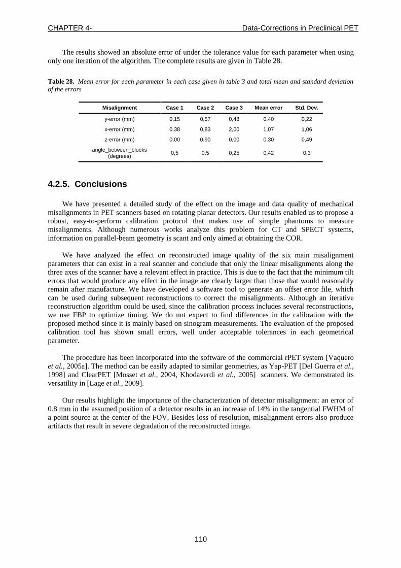
CHAPTER 4- Data-Corrections in Preclinical PET
110
The results showed an absolute error of under the tolerance value for each parameter when using
only one iteration of the algorithm. The complete results are given in Table 28.
Table 28. Mean error for each parameter in each case given in table 3 and total mean and standard deviation
of the errors
Misalignment Case 1 Case 2 Case 3 Mean error Std. Dev.
y-error (mm) 0,15 0,57 0,48 0,40 0,22
x-error (mm) 0,38 0,83 2,00 1,07 1,06
z-error (mm) 0,00 0,90 0,00 0,30 0,49
angle_between_blocks (degrees)
0,5 0,5 0,25 0,42 0,3
4.2.5. Conclusions
We have presented a detailed study of the effect on the image and data quality of mechanical
misalignments in PET scanners based on rotating planar detectors. Our results enabled us to propose a
robust, easy-to-perform calibration protocol that makes use of simple phantoms to measure
misalignments. Although numerous works analyze this problem for CT and SPECT systems,
information on parallel-beam geometry is scant and only aimed at obtaining the COR.
We have analyzed the effect on reconstructed image quality of the six main misalignment
parameters that can exist in a real scanner and conclude that only the linear misalignments along the
three axes of the scanner have a relevant effect in practice. This is due to the fact that the minimum tilt
errors that would produce any effect in the image are clearly larger than those that would reasonably
remain after manufacture. We have developed a software tool to generate an offset error file, which
can be used during subsequent reconstructions to correct the misalignments. Although an iterative
reconstruction algorithm could be used, since the calibration process includes several reconstructions,
we use FBP to optimize timing. We do not expect to find differences in the calibration with the
proposed method since it is mainly based on sinogram measurements. The evaluation of the proposed
calibration tool has shown small errors, well under acceptable tolerances in each geometrical
parameter.
The procedure has been incorporated into the software of the commercial rPET system [Vaquero
et al., 2005a]. The method can be easily adapted to similar geometries, as Yap-PET [Del Guerra et al.,
1998] and ClearPET [Mosset et al., 2004, Khodaverdi et al., 2005] scanners. We demonstrated its
versatility in [Lage et al., 2009].
Our results highlight the importance of the characterization of detector misalignment: an error of
0.8 mm in the assumed position of a detector results in an increase of 14% in the tangential FWHM of
a point source at the center of the FOV. Besides loss of resolution, misalignment errors also produce
artifacts that result in severe degradation of the reconstructed image.
CHAPTER 4- Data-Corrections in Preclinical PET
111
4.3. Attenuation correction of PET images using CT data in the small animal PET scanner Argus PET/CT
Attenuation correction is an important correction required for quantitative analysis of PET.
Although the magnitude of this correction for small animal subjects is much smaller than in humans
[Chow et al., 2002], it is important to correct the data for quantitative analysis of the tracer distribution
[Kinahan et al., 2003].
There are several methods to correct for attenuation in PET [Kinahan et al., 2003, Zaidi et al.,
2004]. The material properties of the object/subject can be obtained using transmission images, which
can be acquired either with a PET or an x-ray CT scanner. For PET transmission, the source is usually
a gamma-emitter isotope (137
Cs for example) while for CT transmission, the source is an X-ray tube.
Even though the transmission image obtained using 137
Cs source provides a good overview of the
structure, the quality of the attenuation correction obtained can be improved further by using an image
obtained from a CT scanner [Chow et al., 2002]. The potential benefits of using CT based attenuation
correction method over the PET based method include: (a) Lower statistical noise in transmission
images acquired on CT versus PET, since the photon flux is higher; (b) availability of high quality
anatomical information; (c) faster acquisitions; (d) less background due to the radioactivity injected to
the patient; (e) transmission scan using PET scanner requires handling of radioactive source. On the
other hand, using CT images to correct the attenuation in PET requires an energy scaling since the
attenuation depends on the photon energy besides on the material properties of the object/subject
[Valk et al., 2006, Kinahan et al., 1998].
In this section we describe a procedure to correct the attenuation based on a CT image for the
SEDECAL Argus PET/CT scanner described in chapter 2, section 2.2. The images are reconstructed
using FIRST code (see chapter 2, section 2.4), but the correction can be used with any other
reconstruction method [Vicente et al., 2010b].
4.3.1. Materials & Methods
4.3.1.1. Mathematical description of the attenuation
The transmission of the photons through the matter can be characterized with the linear
attenuation coefficient, . This coefficient depends on the photon energy E and the atomic number of
the material. A well-collimated mono-energetic beam with an input intensity of I0 passing through a
length of material along any desired line of response (LOR) has an output intensity I of [Valk et al.,
2006]:
LORdx)E,x(
0 eII
(68)
It can be seen from eq. (68) that the photon fraction transmitted through a tissue depends on its
attenuation coefficient and the length of the trajectory.
For PET scanning of homogenous material (), the detection probability (0I
IP ) of
coincidental photon pair is:
DxDx eeeP (69)

CHAPTER 4- Data-Corrections in Preclinical PET
112
where D is the material thickness. Note that the probability that both photons will reach the detector is
independent of the source location along the line of response (Figure 64).
Figure 64. Probability that both photons of a PET coincidence will reach the detectors (A and B), separated a
distance D.
4.3.1.2. Attenuation correction based on a CT image
CT image is a map of the effective linear attenuation coefficient, μ(E), at each point in the body,
and represented as CT numbers in Hounsfield units (HU)
10001)E(
)E(HU
OH2
(70)
The transformation of the CT attenuation coefficient μ(CT) (energies of tens of keV) to μ(PET)
(511 keV) is not completely straightforward. This is because the mechanism of attenuation is different
for energies around 511 keV (with higher probability of Compton) and low energies (where, besides
the Compton scatter, photoelectric absorption and Rayleigh scatter are important contributions as well)
[Valk et al., 2006].
There are several methods to perform this transformation, from the simplest based on a linear
transformation using the attenuation coefficient of water (similar to soft tissue) to the most elaborate
using a detailed segmentation of different tissue types.
In this work we have computed the transformation with a bilinear approximation from the HU
values of air, water and bone (cortical) and the corresponding linear attenuation coefficients () for
photons of 511 keV (Kinahan et al., 1998). The attenuation value for any other material is estimated
using this bilinear transformation and its corresponding HU value (Figure 65).

CHAPTER 4- Data-Corrections in Preclinical PET
113
Figure 65. Bilinear approximation to compute the linear attenuation coefficients.
4.3.1.3. Application of the attenuation correction
The attenuation correction is applied to data before reconstructing the PET images. To carry out
the correction, the attenuation map is forward projected to get the attenuation correction factor (ACF)
for each LOR:
( , )LOR
x E dx
ACF e (71)
The correction is accomplished by multiplying by the ACF of each LOR the data on the same
LOR.
4.3.1.4. Data acquisition and processing
Both acquisitions, PET and CT, were performed using the multimodality scanner Sedecal Argus
PET/CT [Wang et al., 2006b, Vaquero et al., 2008] described in chapter 2, section 2.2. Figure 66
shows a simplified workflow with the necessary steps to correct attenuation in the Argus scanner using
CT images.
Figure 66. Workflow for the attenuation correction using CT images for the SEDECAL Argus PET/CT.

CHAPTER 4- Data-Corrections in Preclinical PET
114
Several phantom studies were performed for validation purposes. In this work we show, as an
example, an acquisition of the NEMA Image quality phantom (more details of the phantom can be
found in Appendix A). The phantom was filled with 18
F except for two small cylindrical cavities
(diameter: 8 mm). One of them was filled with water, and the second one remained empty. The
reconstruction was carried out with FIRST [Herraiz et al., 2006a] with 1 iteration and 50 subsets.
For the Argus scanner, FIRST code includes an attenuation correction of a FOV-sized water
cylinder by default. This default correction is an initial approximation since it does not take into
account the different materials and their distribution in the FOV. In this work we compare the results
of this default correction with the one that we get with a more accurate correction based on a CT
image.
The 2 is a useful parameter in order to verify if the applied corrections or improvement in a
reconstruction algorithm allow for a better description of the data. This quantity is defined as:
LN
1i i
2ii
VL
2
Y
yY
NN
1
(72)
where NL is the number of LORs (independent data acquired), NV is the number of voxels in the
image, being (NL - NV) the degrees of freedom, Yi is the number of counts per LOR, and yi represents
the estimated data, that is, the projection of the object recovered by the reconstruction. High values of
2 imply a disagreement between the estimation and the data and point out inaccuracies in the system
model, failures in the system (a detector not working properly, for instance) and/or some effects not
considered in the reconstruction [Herraiz et al., 2006a].
4.3.2. Results
Figure 67 (top-left) shows the attenuation map for the NEMA Image quality phantom that we got
using the CT image. This map was used to get the ACFs. The second image in Figure 67 is the PET
image with the default attenuation correction, and the next one (top-right) shows the PET image with
the attenuation correction based on the CT image.
Figure 67. NEMA QC phantom analysis. Top, from left to right: Attenuation map obtained from the CT image,
PET image with attenuation correction based on a FOV-sized water cylinder, and PET image with attenuation
correction based on the CT image. Bottom: Normalized profiles through the blue line drawn in the PET images.
FOV-SIZED CORR. CT IMAGE CORR.

CHAPTER 4- Data-Corrections in Preclinical PET
115
The two PET images do not seem to differ significantly to the naked eye, but we can see in a
profile (Figure 67, bottom) through the two small cylindrical cavities (blue dashed line on the PET
images) that there are differences in the air region. If the attenuation correction does not take into
account the different materials in the phantom (as the default correction does, when no CT image is
available), the result is an excess of counts in the air region. The attenuation correction based on the
CT image corrects this problem and after applying it, the two cold regions have a similar number of
counts.
Figure 68 plots the 2 evolution with the number of image updates (number of subsets). We can
see that the attenuation correction based on the CT image reduces sizeably the 2 parameter. This
indicates that the attenuation correction improves the consistency between the reconstructed image and
the acquired data.
Figure 68. 2 evolution with the number of image updates.
Finally, since the procedure has been incorporated into the software of the commercial
Argus PET/CT system, we present in Figure 69 a few screenshots of the 3D-OSEM user
console to show how easy is to perform the correction for a final user. First of all, the user
needs to select, in the ‘upload’ menu (Figure 69A), the acquisition file using the ‘browse’
button. (Figure 69B, ‘Acquisition file to be reconstructed’ label). After that, the user has to
select the attenuation map using the ‘browse’ button (Figure 69C, ‘Attenuation file map’
label). If no attenuation map is selected, the default correction (FOV-sized water cylinder) will
be applied.

CHAPTER 4- Data-Corrections in Preclinical PET
116
(A) (B)
(C)
Figure 69. Screenshots of the 3D-OSEM user console incorporated in the commercial Argus PET/CT
4.3.3. Conclusions
PET data are affected by attenuation which reduces the number of photons detected in each line
of response (LOR). Nowadays, attenuation correction based on CT images is the most practical
method due to the availability of high quality CT images with the low acquisition time.
In this work we have compared a simple attenuation correction method based on a FOV-sized
water cylinder with a more accurate method based on CT images. The attenuation correction based on
CT images not only provides a better quantification, but also reduces the 2 parameter, what means a
better consistency between the reconstructed image and the acquired data. The procedure has been
incorporated into the software of the commercial Argus PET/CT system.

CHAPTER 4- Data-Corrections in Preclinical PET
117
4.4. References Abella, M., Vaquero, J., Soto-Montenegro, M., Lage, E. & Desco, M. 2009. Sinogram Bow-Tie Filtering in FBP PET
Reconstruction. Med. Phys., 36, 1663-71.
Abella, M., Vaquero, J. J., Vicente, E., Álvarez, J., Lage, E. & Desco, M. 2006. Effect of misalignments in small animal PET
scanners based on rotating planar detectors. Mol. Ima. Biol., 8, 75-6.
Abella, M., Vicente, E., Rodríguez-Ruano, A., España, S., Lage, E., Desco, M., Udias, J. M. & Vaquero, J. J. 2012.
Misalignments calibration in small-animal PET scanners based on rotating planar detectors and parallel-beam
geometry. Phys Med Biol (Submitted).
Azevedo, S. G., Schneberk, D. J., Fitch, J. P. & Martz, H. E. 1990. Calculation of the rotational centers in computed
tomography sinograms. Nuclear Science, IEEE Transactions on, 37, 1525-1540.
Badawi, R. D. & Marsden, P. K. 1999b. Self-normalization of emission data in 3D PET. IEEE Transactions on Nuclear
Science, 46, 709-712.
Badawi, R. D., Miller, M. P., Bailey, D. L. & Marsden, P. K. 1999. Randoms variance reduction in 3D PET. Phys Med Biol,
44, 941-54.
Bendriem, B. & Townsend, D. W. 1998. The theory and practice of 3D PET. Kluwer Academic.
Beque, D., Nuyts, J., Bormans, G., Suetens, P. & Dupont, P. 2003. Characterization of pinhole SPECT acquisition geometry.
IEEE Trans. Med. Imaging, 22, 599–612.
Brasse, D., Kinahan, P. E., Lartizien, C., Comtat, C., Casey, M. & Michel, C. 2005. Correction methods for random
coincidences in fully 3D whole-body PET: impact on data and image quality. J Nucl Med, 46, 859-67.
Busemann-Sokole, E. 1987. Measurement of collimator hole angulation and camera head tilt for slant and parallel-hole
collimators used in SPECT. J. Nucl. Med., 28, 1592–8.
Casey, M. E. & Hoffman, E. J. 1986. Quantitation in positron emission computed tomography: 7. A technique to reduce
noise in accidental coincidence measurements and coincidence efficiency calibration. J Comput Assist Tomogr, 10,
845-50.
Cherry, S. R., Sorenson, J. A. & Phelps, M. E. 2003. Physics in nuclear medicine, Saunders.
Chow, P. L., Rannou, R. & Chatziioannou, A. 2002. Attenuation correction for a 3D small animal PET tomograph, using x-
ray microCT. Mol. Imag. Biol., 4, S17–S18.
Daube-Witherspoon, M. E. & Carson, R. E. 1991. Unified deadtime correction model for PET. IEEE Trans Med Imaging, 10,
267-75.
Del Guerra, A., Di Domenico, G., Scandola, M. & Zavattini, G. 1998. YAP-PET: first results of a small animal positron
emission tomograph based on YAP:Ce finger crystals. Nuclear Science, IEEE Transactions on, 45, 3105-3108.
Donath, T., Beckmann, F. & Schreyer, A. 2006. Automated determination of the center of rotation in tomography data. J.
Opt. Soc. Am., 23, 1048-1057.
Eriksson, L., Wienhard, K. & Dahlbom, M. 1994 A simple data loss model for positron camera systems. IEEE Transactions
on Nuclear Science, 41, 1566 - 1570
España, S., Herraiz, J. L., Vicente, E., Vaquero, J. J., Desco, M. & Udias, J. M. 2009. PeneloPET, a Monte Carlo PET
simulation tool based on PENELOPE: features and validation. Phys Med Biol, 54, 1723-42.
Furrer, M., Gostely, J. J. & Lerch, P. 1984. Timing problems due to pile-up in coincidence counting. Nuclear Instruments
and Methods in Physics Research Section A: Accelerators, Spectrometers, Detectors and Associated Equipment,
226, 455-462.
Germano, G. & Hoffman, E. J. 1988. Investigation of count rate and deadtime characteristics of a high resolution PET
system. J Comput Assist Tomogr, 12, 836-46.
Germano, G. & Hoffman, E. J. 1990. A study of data loss and mispositioning due to pileup in 2-D detectors in PET.
Germano, G. & Hoffman, E. J. 1991. An investigation of methods of pileup rejection for 2-D array detectors employed in
high resolution PET. IEEE Trans Med Imaging, 10, 223-7.
Gullberg, G. T., Tsui, B. M. W., Crawford, C. R., Ballard, J. G. & Hagius, J. T. 1990. Estimation of geometrical parameters
and collimator evaluation for cone beam tomography. Med. Phys., 17, 264–72.
Gullberg, G. T., Tsui, B. M. W., Crawford, C. R. & Edgerton, E. 1987. Estimation of geometrical parameters for fan-beam
tomography. Phys. Med. Biol., 32, 1581–94.
Herraiz, J. L., Espana, S., Vaquero, J. J., Desco, M. & Udias, J. M. 2006a. FIRST: Fast Iterative Reconstruction Software for
(PET) tomography. Phys Med Biol, 51, 4547-65.
Hoffman, E. J., Phelps, M. E. & Huang, S. C. 1983. Performance evaluation of a positron tomograph designed for brain
imaging. J Nucl Med, 24, 245-57.
Hsieh, Y.-L. 1992. Calibration of fan-beam geometry for single photon emission computed tomography. University of Utah.
Imperiale, C. & Imperiale, A. 2001. On nuclear spectrometry pulses digital shaping and processing. Measurement, 30, 49-73.
Jagoda, E. M., Vaquero, J. J., Seidel, J., Green, M. V. & Eckelman, W. C. 2004. Experiment assessment of mass effects in
the rat: implications for small animal PET imaging. Nuclear Medicine and Biology, 31, 771-9.
Khodaverdi, M., Weber, S., Streun, M., Parl, C., Larue, H., Brandenburg, G., Bauer, A., Dehnhardt, M., Auffray, E.,
Boutemeur, M., Bruyndonckx, P., Choi, Y., D'Asseler, Y., Devroede, O., Dujardin, C., Fedorov, A., Heinrichs, U.,
Janier, M., Jung, J. H., Korjik, M., Krieguer, M., Largeron, G., Lartizien, C., Lecoq, P., Lemaitre, C., Leonard, S.,
Loude, J. F., Morel, C., Mosset, J. B., Pedrini, C., Petrosyan, A. G., Rey, M., Sappey-Marinier, D., Roldan, P. S.,
Simon, L., Song, T. Y., Staelens, S., Tavernier, S., Trummer, J., Van Holen, R., Vieira, J. M., Wieers, E.,
Wisniewska, M., Wisniewski, D., Wu, Y., Pietrzyk, U. & Ziemons, K. 2005. High resolution imaging with
ClearPET™ Neuro - first animal images. In: Nuclear Science Symposium Conference Record, 2005 IEEE,

CHAPTER 4- Data-Corrections in Preclinical PET
118
23-29 Oct. 2005 2005. 4 pp.
Kinahan, P. E., Hasegawa, B. H. & Beyer, T. 2003. X-ray-based attenuation correction for positron emission
tomography/computed tomography scanners. Semin Nucl Med, 33, 166-79.
Kinahan, P. E., Townsend, D. W., Beyer, T. & Sashin, D. 1998. Attenuation correction for a combined 3D PET/CT scanner.
Med Phys, 25, 2046-53.
Knoll, G. F. 2000. Radiation detection and measurement / Glenn F. Knoll, New York :, Wiley.
Lage, E., Vaquero, J. J., Sisniega, A., Espana, S., Tapias, G., Abella, M., Rodriguez-Ruano, A., Ortuno, J. E., Udias, A. &
Desco, M. 2009. Design and performance evaluation of a coplanar multimodality scanner for rodent imaging. Phys
Med Biol, 54, 5427-41.
Lecomte, R. 2004. Technology challenges in small animal PET imaging. Nucl. Instrum. Meth. Phys. Res. A, 527, 157-165.
Lewis, J. S. & Achilefu, S. 2002. Small Animal Imaging: Current Technology and Perpectives for Oncological Imaging. Eur.
J. Cancer, 38, 2173-88.
Mankoff, D. A., Muehllehner, G. & Karp, J. S. 1989. The high count rate performance of a two-dimensionally position-
sensitive detector for positron emission tomography. Phys Med Biol, 34, 437-56.
Massoud, T. F. & Gambhir, S. S. 2003. Molecular imaging in living subjects: seeing fundamental biological processes in a
new light. Gene. Dev., 17, 545-80.
Mazoyer, B. M., Roos, M. S. & Huesman, R. H. 1985. Dead time correction and counting statistics for positron tomography.
Phys Med Biol, 30, 385-99.
Mosset, J. B., Devroede, O., Krieguer, M., Rey, M., Vieira, J. M., Jung, J. H., Kuntner, C., Streun, M., Ziemons, K., Auffray,
E., Sempere-Roldan, P., Lecoq, P., Bruyndonckx, P., Loude, J. F., Tavernier, S. & Morel, C. 2004. Development of
an optimised LSO/LuYAP phoswich detector head for the ClearPET camera. In: Nuclear Science Symposium
Conference Record, 2004 IEEE, 16-22 Oct. 2004 2004. 2439-2443 Vol. 4.
Noo, F., Clackdoyle, R., Mennessier, C., White, T. A. & Roney, T. J. 2000. An analytic method based on identification of
ellipse parameters for scanner calibration in conebeam tomography. Phys. Med. Biol., 45, 3489-3508.
Pierce, L., Miyaoka, R., Lewellen, T., Alessio, A. & Kinahan, P. 2009. Determining Block Detector Positions for PET
Scanners. IEEE Nucl. Sci. Symp. Conf. Rec.
Pomper, M. G. 2001. Molecular Imaging: and Overview. Acad. Radiol., 8, 1141-53.
Seidel, J., Wenze, X., Kakareka, J. W., Pohida, T. J., Green, M. V. & Choyke, P. L. 2010. A positron projection imager for
whole-body mouse imaging. In: Nuclear Science Symposium Conference Record (NSS/MIC), 2010 IEEE, Oct. 30
2010-Nov. 6 2010 2010. 2206-2209.
Sjöland, K. A. & Kristiansson, P. 1994. Pile-up and defective pulse rejection by pulse shape discrimination in surface barrier
detectors. Nuclear Instruments and Methods in Physics Research Section B: Beam Interactions with Materials and
Atoms, 94, 333-337.
Smith, R. J., Karp, J. S. & Muehllehner, G. 1994. The countrate performance of the volume imaging PENN-PET scanner.
IEEE Trans Med Imaging, 13, 610-8.
Stearns, C. W., Chesler, D. A., Kirsch, J. E. & Brownell, G. L. 1985. Quantitative Imaging with the MGH Analog Ring
Positron Tomograph. IEEE Transactions on Nuclear Science, 32, 898-901.
Stearns, C. W., McDaniel, D. L., Kohlmyer, S. G., Arul, P. R., Geiser, B. P. & Shanmugam, V. 2003. Random coincidence
estimation from single event rates on the Discovery ST PET/CT scanner. In: Nuclear Science Symposium
Conference Record, 2003 IEEE, 19-25 Oct. 2003 2003. 3067-3069 Vol.5.
Sun, Y., Hou, Y. & Hu, J. 2007. Reduction of Artifacts Induced by Misaligned Geometry in Cone-Beam CT. IEEE Trans.
Bio. Eng., 54, 1461-71.
Thompson, C. J. & Meyer, E. 1987. The effect of live time in components of a positron tomograph on image quantification.
Valk, P. E., Delbeke, D. & Bailey, D. L. 2006. Positron emission tomography: clinical practice, Springer.
Vaquero, J. J., Lage, E., Ricon, L., Abella, M., Vicente, E. & Desco, M. 2005a. rPET detectors design and data processing.
In: Nuclear Science Symposium Conference Record, 2005 IEEE, 23-29 Oct. 2005 2005a. 2885-2889.
Vaquero, J. J., Lage, E., Ricón, L., Abella, M., Vicente, E. & Desco, M. 2005b. rPET Detectors Design and Data Processing.
IEEE Nuclear Science Symposium Conference Record.
Vaquero, J. J., Redondo, S., Lage, E., Abella, M., Sisniega, A., Tapias, G., Montenegro, M. L. S. & Desco, M. 2008.
Assessment of a New High-Performance Small-Animal X-Ray Tomograph. Nuclear Science, IEEE Transactions
on, 55, 898-905.
Vicente, E., Espana, S., Lopez Herraiz, J., Herranz, E., Desco, M., Vaquero, J. J. & Udias, J. M. 2008. Nonlinear effect of
pile-up in the quantification of a small animal PET scanner. In: Nuclear Science Symposium Conference Record,
2008. NSS '08. IEEE, 19-25 Oct. 2008 2008. 5391-5395.
Vicente, E., Herraiz, J. L., Espana, S., Herranz, E., Desco, M., Vaquero, J. J. & Udias, J. M. 2011. Deadtime and pile-up
correction method based on the singles to coincidences ratio for PET. In: Nuclear Science Symposium and
Medical Imaging Conference (NSS/MIC), 2011 IEEE, 23-29 Oct. 2011 2011. 2933-2935.
Vicente, E., Herraiz, J. L., España, S., Herranz, E., Desco, M., Vaquero, J. J. & Udías, J. M. 2012a. Improved effective dead-
time correction for PET scanners: Application to small-animal PET. Phys Med Biol (Submitted).
Vicente, E., Soto-Montenegro, M., España, S., Herraiz, J. L., Herranz, E., Vaquero, J. J., Desco, M. & Udias, J. M. 2007.
Influence of random, pile-up and scatter corrections in the quantification properties of small-animal PET scanners.
In: Nuclear Science Symposium Conference Record, 2007. NSS '07. IEEE, Oct. 26 2007-Nov. 3 2007 2007. 3964-
3968.
Vicente, E., Udías, A. L., Herraiz, J. L., Desco, M., Vaquero, J. J. & Udías, J. M. 2010b. Corrección de atenuación de
imágenes PET usando datos de TAC en el escáner para animales pequeños Argus PET/CT. Libro de Actas,
CASEIB 2010.
Wang, G. C., Huber, J. S., Moses, W. W., Qi, J. & Choong, W. S. 2006a. Characterization of the LBNL PEM camera.

CHAPTER 4- Data-Corrections in Preclinical PET
119
Nuclear Science, IEEE Transactions on, 53, 1129-1135.
Wang, Y., Seidel, J., Tsui, B. M., Vaquero, J. J. & Pomper, M. G. 2006b. Performance evaluation of the GE healthcare
eXplore VISTA dual-ring small-animal PET scanner. J Nucl Med, 47, 1891-900.
Williams, C. W., Crabtree, M. C. & Burgiss, S. G. 1979. Design and Performance Characteristics of a Positron Emission
Computed Axial Tomograph--ECAT®-II. Nuclear Science, IEEE Transactions on, 26, 619-627.
Wu, Y., Bowen, S. L., Yang, K., Packard, N., Fu, L., Burkett, G., Qi, J., Boone, J. M., Cherry, S. R. & Badawi, R. D. 2009.
PET characteristics of a dedicated breast PET/CT scanner prototype. Phys Med Biol, 54, 4273-87.
Yamamoto, S., Amano, M., Miura, S., Iida, H. & Kanno, I. 1986. Deadtime correction method using random coincidence for
PET. J Nucl Med, 27, 1925-8.
Zaidi, H., Montandon, M. L. & Slosman, D. O. 2004. Attenuation compensation in cerebral 3D PET: effect of the attenuation
map on absolute and relative quantitation. Eur J Nucl Med Mol Imaging, 31, 52-63.
Zhang, H., Bao, Q., Vu, N. T., Silverman, R. W., Taschereau, R., Berry-Pusey, B. N., Douraghy, A., Rannou, F. R., Stout, D.
B. & Chatziioannou, A. F. 2011. Performance evaluation of PETbox: a low cost bench top preclinical PET scanner.
Mol Imaging Biol, 13, 949-61.

CHAPTER 4- Data-Corrections in Preclinical PET
120

CHAPTER 5- Design of Small Animal PET Prototypes
121
5. Design of Small Animal PET Prototypes
Small animal PET tomographs play an important role in biology [Myers, 2001, Herschman, 2003]
and studies of in vivo tracer pharmacokinetics and metabolism [Wang and Maurer, 2005, Sossi and
Ruth, 2005, Toyama et al., 2005, Kenanova et al., 2007]. Pavlopoulos and Tzanakos [Pavlopoulos and
Tzanakos, 1993, 1996] were among the first to suggest, in 1992, a small animal PET with highly
segmented detector blocks [Tzanakos and Pavlopoulos, 1993], based on BGO and a new position
sensitive photomultiplier (PSPMT), the Hamamatsu R2487. Theirs was a computer aided design made
possible by the use of a newly developed Monte Carlo package [Tzanakos and Pavlopoulos, 1991],
which simulated the individual blocks as well as the whole PET system. Other Monte Carlo packages
designed for special studies in PET appeared in the literature at the same time [Thompson et al.,
1992a]. Soon, the first realization of a small animal PET scanner by Watanabe et al. was published in
[Watanabe et al., 1992].
Ever since this first small animal PET system appeared, small animal PET scanners are in
continuous development. New systems are produced with higher sensitivity, spatial resolution, and
count rate capabilities [Wang et al., 2006b, Bao et al., 2009a]. The design of a new small animal PET
scanner is a very complex process that requires taking decisions of several natures. Monte Carlo
simulation have turned into an invaluable tool for all the stages of the PET scanners design, allowing
for exhaustive studies which take into account all the elements of the scanner [Heinrichs et al., 2003].
A considerable number of Monte Carlo packages with different characteristics are available
nowadays, suitable for the simulation of either PET or SPECT physical processes, with different detail
level [Rogers, 1984, Briesmeister, 1993, Baró et al., 1995, Agostinelli, 2003, Harrison et al., 1993, Jan
et al., 2004b, Zaidi and Scheurer, 1999, Thompson et al., 1992b, España et al., 2009]. Although most
of these packages are very flexible, it is virtually impossible that they cover every conceivable
variation of design of a PET scanner. Thus it is often necessary to introduce extensions in the MC
codes to make them able of simulating non-standard geometries of some prototypes.
Besides the simulation of raw data, it is necessary to develop appropriate reconstruction methods
to process this data in order to evaluate the performance of the system, such as the spatial resolution,
and to assess the quality of the final images. To this end, existing reconstruction methods have to be
modified and extended to adapt the existing codes to the non-conventional geometry of some designs.
Examples of these modifications on simulation and reconstruction codes to suit particularly
creative or non-standard geometries are presented in this chapter whose purpose is the study, by means
of Monte Carlo simulations, of the main features and fine tune of design of two new small animal PET
prototypes under development in two different centers where the author of this thesis was working as a
part of an internship program. The two studied prototypes are:
Zoom-in PET system (section 5.1), proposed and designed by the Department of Biomedical
Engineering, University of California, (Davis, CA, USA) [Zhou and Qi, 2009, 2010, 2011, Qi
et al., 2011]. The system incorporates a high-resolution detector into an existing PET scanner
to obtain high-resolution images of a region of interest.
NIH PPI system (section 5.2) developed at the National Institutes of Health (NIH), Bethesda,
MD, USA (Molecular Imaging Program, National Cancer Institute) [Seidel et al., 2010]. It is a
low cost bench top preclinical PET scanner dedicated to mouse studies which employs a non-
rotating compact dual-head geometry similar to those of positron emission mammography
(PEM) systems.
CHAPTER 5- Design of Small Animal PET Prototypes
122
5.1. Zoom-in PET scanner
Small animal PET systems have been improved significantly in terms of spatial resolution and
sensitivity since their first development in the mid 1990s. Images with higher resolution can improve
our capability of studying human diseases using animal models. For instance, sub-millimeter
resolution is required in order to detect small metastases or study brain function in mice. This explain
the never ending quest for improved resolution in small animal PET scanners.
Most current systems use scintillator-based detectors because of their ability to achieve high
performance with a relatively compact geometry and at an acceptable cost [Chatziioannou, 2002].
Some research systems have reported sub-millimeter spatial resolutions in animal studies using arrays
of small scintillator elements [Tai et al., 2003, Rouze et al., 2004, Miyaoka et al., 2005]. However, the
resolution of these systems is still mainly limited by the physical size of the scintillator elements and
the intrinsic spatial resolution of the detectors [Stickel and Cherry, 2005]. Using smaller scintillator
elements in close proximity to the object is useful to obtain both higher spatial resolution and
sensitivity, but one has to keep in mind that these two performance goals (high resolution and high
sensitivity) are in competency. Simulations help to decide the best tradeoff between resolution and
sensitivity. Successful instances have been presented where high-resolution detectors are either
inserted into an existing whole body PET scanner [Janecek et al., 2006, Wu et al., 2008c] or a small-
animal PET device prepared to be as close as possible to the object being imaged [Clinthorne et al.,
2003, Park et al., 2007, Wu et al., 2008b] to improve the system performance in a smaller field of
view (FOV). The effect of high-resolution inserts on system resolution was analyzed by [Tai et al.,
2008]. Related work on modeling of a half-ring PET insert was presented in [Keesing et al., 2008].
While these approaches have been successful, there is clearly room for improvement. First, most
PET-inserts require a large number of high-resolution detectors (either partial or full ring) to be placed
within the gantry of an existing system, which significantly increases the complexity of the system
(e.g., number of electronic channels) and the cost. Second, most existing PET inserts use short
scintillation crystals (e.g., 3.75 mm for the micro-insert described in [Wu et al., 2008b]) to avoid the
depth of interaction (DOI) effect, yielding a fairly low sensitivity for the high-resolution detector,
which limits the potential gain of using the insert. In addition, high-resolution detectors are usually
placed in a ring at a fixed radius, so it may not be possible to position the animal right up against the
high-resolution detectors to take full advantage of the resolution available.
In this section we study a new prototype, the ‘Zoom-in PET’ system (or ZiPET), proposed and
designed by the Department of Biomedical Engineering, University of California, (Davis, CA) [Zhou
and Qi, 2009, 2010, 2011, Qi et al., 2011], where the author of this thesis was working during the
summer of 2010. The system integrates a single high-resolution detector into an existing microPET
scanner that acts analogously to a ‘magnifying glass’ in order to obtain high-resolution data of a small
portion of the FOV defined by a region of interest around the face of the insert (see Figure 70). The
proposed design can offer a cost-effective solution to obtain high-resolution images for a targeted
region without building a full-ring PET system. Such a system can be useful for studying human
tumors with animal models where tumors are often grown near the surface of the skin of the animal
and therefore they can be placed very close to the high-resolution detector.
In this work we use Monte Carlo simulations with PeneloPET (see chapter 2, section 2.3) to
characterize the impact of the insert in the performance of the system. It was necessary to introduce
several modifications in the PeneloPET code due to the non-standard geometry of the system with two
different sets of block detectors at different radial positions. The improvement in spatial resolution was
already studied in previous works using theoretical analysis and basic simulations [Zhou and Qi,
2009], and experimental measurements [Qi et al., 2011].
This section is organized as follows. Section 5.1.1 describes in detail the setup of the ZiPET
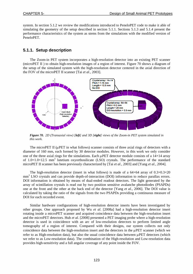
CHAPTER 5- Design of Small Animal PET Prototypes
123
system. In section 5.1.2 we review the modifications introduced to PeneloPET code to make it able of
simulating the geometry of the setup described in section 5.1.1. Sections 5.1.3 and 5.1.4 present the
performance characteristics of the system as stems from the simulations with the modified version of
PeneloPET.
5.1.1. Setup description
The Zoom-in PET system incorporates a high-resolution detector into an existing PET scanner
(microPET II ) to obtain high-resolution images of a region of interest. Figure 70 shows a diagram of
the setup of the simulated system with the high-resolution detector centered in the axial direction of
the FOV of the microPET II scanner [Tai et al., 2003].
Figure 70. 2D (Transaxial view) [left] and 3D [right] views of the Zoom-in PET system simulated in
this work.
The microPET II (PET in what follows) scanner consists of three axial rings of detectors with a
diameter of 160 mm, each formed by 30 detector modules. However, in this work we only consider
one of the three axial rings for the simulations. Each PET detector module consists of a 14×14 array
of 1.0×1.0×12.5 mm3 lutetium oxyorthosilicate (LSO) crystals. The performance of the standard
microPET II scanner has been previously characterized by [Tai et al., 2003] and [Yang et al., 2004].
The high-resolution detector (insert in what follows) is made of a 64×64 array of 0.3×0.3×20
mm3 LSO crystals and can provide depth-of-interaction (DOI) information to reduce parallax errors.
DOI information is obtained by means of dual-ended readout detectors. The light generated by the
array of scintillation crystals is read out by two position sensitive avalanche photodiodes (PSAPDs)
one at the front and the other at the back end of the detector [Yang et al., 2006]. The DOI value is
calculated by taking the ratio of the signals from the two PSAPDs providing a continuous measure of
DOI for each recorded event.
Similar hardware configurations of high-resolution detector inserts have been investigated by
other groups. One approach proposed by Wu et al. [2008a] had a high-resolution detector insert
rotating inside a microPET scanner and acquired coincidence data between the high-resolution insert
and the microPET detectors. Huh et al. [2008] presented a PET imaging probe where a high-resolution
detector is used in coincidence with an arc of low-resolution detectors to perform limited angle
tomography of a region of interest. Compared with their designs, our system collects not only
coincidence data between the high-resolution insert and the detectors in the PET scanner (which we
refer to as High-resolution data), but also the usual coincidence data between PET detectors (which
we refer to as Low-resolution data). The combination of the High-resolution and Low-resolution data
provides high-sensitivity and a full angular coverage of any point inside the FOV.
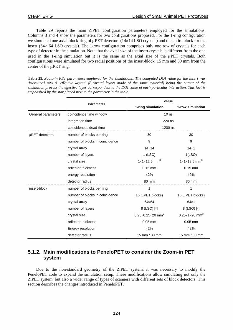
CHAPTER 5- Design of Small Animal PET Prototypes
124
Table 29 reports the main ZiPET configuration parameters employed for the simulations.
Columns 3 and 4 show the parameters for two configurations proposed. For the 1-ring configuration
we simulated one axial block-ring of PET detectors (1414 LSO crystals) and the entire block for the
insert (64 64 LSO crystals). The 1-row configuration comprises only one row of crystals for each
type of detector in the simulation. Note that the axial size of the insert crystals is different from the one
used in the 1-ring simulation but it is the same as the axial size of the PET crystals. Both
configurations were simulated for two radial positions of the insert-block, 15 mm and 30 mm from the
center of the PET ring.
Table 29. Zoom-in PET parameters employed for the simulations. The computed DOI value for the insert was
discretized into 8 ‘effective layers’ (8 virtual layers made of the same material) being the output of the
simulation process the effective layer correspondent to the DOI value of each particular interaction. This fact is
emphasized by the star placed next to the parameter in the table.
Parameter
value
1-ring simulation 1-row simulation
General parameters coincidence time window 10 ns
integration time 220 ns
coincidences dead-time 1200 ns
PET detectors number of blocks per ring 30 30
number of blocks in coincidence 9 9
crystal array 1414 141
number of layers 1 (LSO) 1(LSO)
crystal size 1112.5 mm3 1112.5 mm
3
reflector thickness 0.15 mm 0.15 mm
energy resolution 42% 42%
detector radius 80 mm 80 mm
insert-block number of blocks per ring 1 1
number of blocks in coincidence 15 (PET blocks) 15 (PET blocks)
crystal array 6464 641
number of layers 8 (LSO) [*] 8 (LSO) [*]
crystal size 0.250.2520 mm3 0.25120 mm
3
reflector thickness 0.05 mm 0.05 mm
Energy resolution 42% 42%
detector radius 15 mm / 30 mm 15 mm / 30 mm
5.1.2. Main modifications to PeneloPET to consider the Zoom-in PET system
Due to the non-standard geometry of the ZiPET system, it was necessary to modify the
PeneloPET code to expand the simulation setup. These modifications allow simulating not only the
ZiPET system, but also a wider range of types of scanners with different sets of block detectors. This
section describes the changes introduced in PeneloPET.
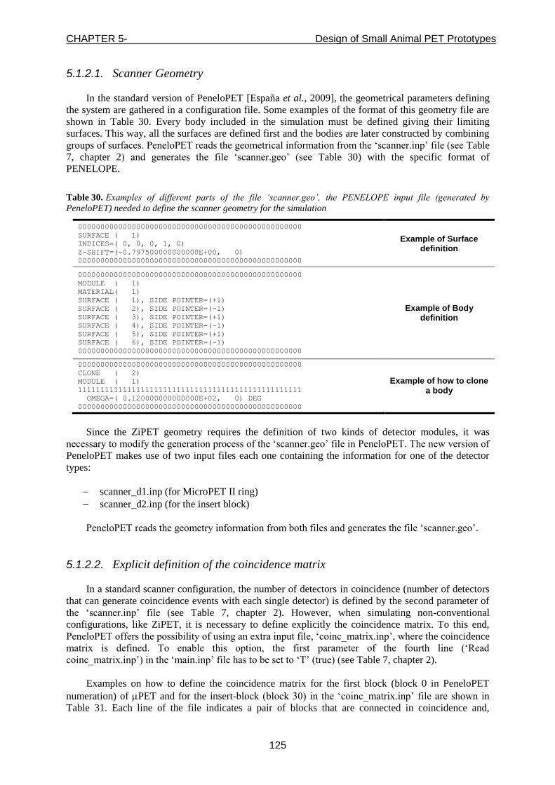
CHAPTER 5- Design of Small Animal PET Prototypes
125
5.1.2.1. Scanner Geometry
In the standard version of PeneloPET [España et al., 2009], the geometrical parameters defining
the system are gathered in a configuration file. Some examples of the format of this geometry file are
shown in Table 30. Every body included in the simulation must be defined giving their limiting
surfaces. This way, all the surfaces are defined first and the bodies are later constructed by combining
groups of surfaces. PeneloPET reads the geometrical information from the ‘scanner.inp’ file (see Table
7, chapter 2) and generates the file ‘scanner.geo’ (see Table 30) with the specific format of
PENELOPE.
Table 30. Examples of different parts of the file ‘scanner.geo’, the PENELOPE input file (generated by
PeneloPET) needed to define the scanner geometry for the simulation
00000000000000000000000000000000000000000000000000
SURFACE ( 1)
INDICES=( 0, 0, 0, 1, 0)
Z-SHIFT=(-0.797500000000000E+00, 0)
00000000000000000000000000000000000000000000000000
Example of Surface definition
00000000000000000000000000000000000000000000000000
MODULE ( 1)
MATERIAL( 1)
SURFACE ( 1), SIDE POINTER=(+1)
SURFACE ( 2), SIDE POINTER=(-1)
SURFACE ( 3), SIDE POINTER=(+1)
SURFACE ( 4), SIDE POINTER=(-1)
SURFACE ( 5), SIDE POINTER=(+1)
SURFACE ( 6), SIDE POINTER=(-1)
00000000000000000000000000000000000000000000000000
Example of Body definition
00000000000000000000000000000000000000000000000000
CLONE ( 2)
MODULE ( 1)
11111111111111111111111111111111111111111111111111
OMEGA=( 0.120000000000000E+02, 0) DEG
00000000000000000000000000000000000000000000000000
Example of how to clone a body
Since the ZiPET geometry requires the definition of two kinds of detector modules, it was
necessary to modify the generation process of the ‘scanner.geo’ file in PeneloPET. The new version of
PeneloPET makes use of two input files each one containing the information for one of the detector
types:
scanner_d1.inp (for MicroPET II ring)
scanner_d2.inp (for the insert block)
PeneloPET reads the geometry information from both files and generates the file ‘scanner.geo’.
5.1.2.2. Explicit definition of the coincidence matrix
In a standard scanner configuration, the number of detectors in coincidence (number of detectors
that can generate coincidence events with each single detector) is defined by the second parameter of
the ‘scanner.inp’ file (see Table 7, chapter 2). However, when simulating non-conventional
configurations, like ZiPET, it is necessary to define explicitly the coincidence matrix. To this end,
PeneloPET offers the possibility of using an extra input file, ‘coinc_matrix.inp’, where the coincidence
matrix is defined. To enable this option, the first parameter of the fourth line (‘Read
coinc_matrix.inp’) in the ‘main.inp’ file has to be set to ‘T’ (true) (see Table 7, chapter 2).
Examples on how to define the coincidence matrix for the first block (block 0 in PeneloPET
numeration) of PET and for the insert-block (block 30) in the ‘coinc_matrix.inp’ file are shown in
Table 31. Each line of the file indicates a pair of blocks that are connected in coincidence and,

CHAPTER 5- Design of Small Animal PET Prototypes
126
therefore, can generate coincidence events. One block can be in coincidence with as many blocks as
desired. It is important to remark that, once the coincidence matrix option has been enabled, only the
detectors specified in the file will be connected in coincidence, ignoring all other possible connections.
Table 31. Examples of coincidence matrix definition for the first block (block 0) of PET and for the insert-
block (block 30) in the ‘coinc_matrix.inp’ file (first column of the table). Second column of the table shows a
graphic example of the pair of blocks in coincidence (red lines) defined in the first column.
Coincidences pairs for the block 0
Coincidences for the block 30 (insert)
5.1.2.3. Dynamic loading of detector parameters for each single detection
In the standard version of PeneloPET, detector parameters are treated as global variables which
are used in all the computations involving radiation interaction in the detectors. Since ZiPET has two
kinds of detectors, it was necessary to dynamically detect the type of detector involved in the
interaction and load the appropriate parameters every time a photon interacted with a detector block. A
flowchart of the procedure is shown in Figure 71:
Figure 71. Flowchart of the new procedure of identifying the type of block-detector and loading its parameters.
NO photon interaction in the insert-block
Identification of the detection position
(type of block)
Both photons
detected by PET
ring
PET block – insert coincidence
One photon interacts in the insert-block
Load PET-block parameters for both
detectors in coincidence
Load PET and insert-block
parameters for each corresponding
detector in coincidence
Detection step (interaction of photons
with the block-detectors
of the scanner)
Store LOR in Low-resolution
output data
Store LOR in High-resolution
output data
LOR determination

CHAPTER 5- Design of Small Animal PET Prototypes
127
5.1.2.4. DOI modeling
To model the effect of DOI as estimated in the insert-block, the depth of interaction inside the
insert of each event was blurred using a convolution with a Gaussian kernel..The use of a Gaussian
kernel is justified based on measurements of DOI distributions from experimental detectors [James et
al., 2009, Yang et al., 2006]. For an actual DOI Z (obtained from PENELOPE) in the crystal, the
blurred depth Z’ is given by:
where Z is obtained from a zero-mean normal distribution with standard deviation, σ, chosen to
match the FWHM of the Gaussian distribution to the DOI resolution. This yields:
The resulting depth in the detector, Z’, must be limited to the physical length of the scintillation
crystals (20 mm), thus events that after DOI blurring would be located outside of the crystal are placed
at 0 or 20 mm depth, as appropriate.
In our simulations, the DOI resolution employed to shift the original estimation of DOI in
PeneloPET was 2.5 mm. Having this value and given the crystal length, the value of Z’ for each
interaction was binned into 8 ‘effective layers’, being the output of the simulation process the effective
layer correspondent to the Z’ value of every interaction.
5.1.2.5. New output files for High and Low resolution data
The ZiPET system collects the coincidence data between the high-resolution detector and the
detectors in the PET scanner (High-resolution data), and also the projection data between PET
detectors (Low-resolution data). For this reason, to provide a detailed analysis of the data and get high-
resolution reconstructed images, different output files with separated High/Low resolution data were
added to the default output files.
5.1.3. Simulated study of the performance of the scanner
In order to study the potential of the ZiPET system, we evaluate three key performance
characteristics for the different configurations in Table 29, namely the sensitivity, the DOI capability
of the insert-block and the noise equivalent count (NEC) rate.
5.1.3.1. Sensitivity
The sensitivity of the system was estimated from simulations of point sources placed at different
positions within the FOV. First we evaluated the absolute central point sensitivity (ACS) for the
configurations described in Table 29 to investigate the increase in sensitivity provided by the use of
the insert compared to the sole PET ring and the improvement when using the whole ring as
compared to a single row of crystals. The statistic of coincidence event types (trues, scatter, randoms,
pile-up, etc.) was also studied.
In order to study in more detail the improvement in sensitivity due to the insert, we simulated
point sources at several positions distributed along the X direction (red arrow in Figure 72) for the
radial position of the insert of 1.5 cm. This setup was selected to mimic the conditions used to measure
(73)
(74)
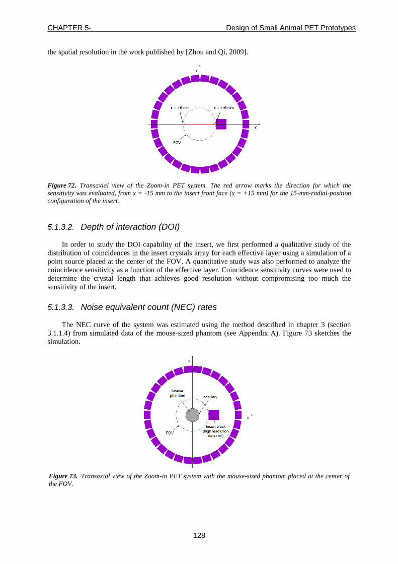
CHAPTER 5- Design of Small Animal PET Prototypes
128
the spatial resolution in the work published by [Zhou and Qi, 2009].
Figure 72. Transaxial view of the Zoom-in PET system. The red arrow marks the direction for which the
sensitivity was evaluated, from x = -15 mm to the insert front face (x = +15 mm) for the 15-mm-radial-position
configuration of the insert.
5.1.3.2. Depth of interaction (DOI)
In order to study the DOI capability of the insert, we first performed a qualitative study of the
distribution of coincidences in the insert crystals array for each effective layer using a simulation of a
point source placed at the center of the FOV. A quantitative study was also performed to analyze the
coincidence sensitivity as a function of the effective layer. Coincidence sensitivity curves were used to
determine the crystal length that achieves good resolution without compromising too much the
sensitivity of the insert.
5.1.3.3. Noise equivalent count (NEC) rates
The NEC curve of the system was estimated using the method described in chapter 3 (section
3.1.1.4) from simulated data of the mouse-sized phantom (see Appendix A). Figure 73 sketches the
simulation.
Figure 73. Transaxial view of the Zoom-in PET system with the mouse-sized phantom placed at the center of
the FOV.
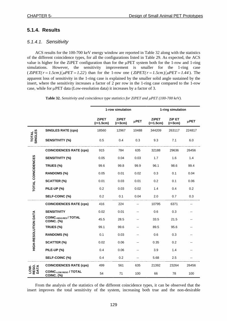
CHAPTER 5- Design of Small Animal PET Prototypes
129
5.1.4. Results
5.1.4.1. Sensitivity
ACS results for the 100-700 keV energy window are reported in Table 32 along with the statistics
of the different coincidence types, for all the configurations listed in Table 29. As expected, the ACS
value is higher for the ZiPET configuration than for the PET system both for the 1-row and 1-ring
simulations. However, the sensitivity improvement is smaller for the 1-ring case
( 22.1PET)cm5.1r(ZiPET ) than for the 1-row one ( 44.1PET)cm5.1r(ZiPET ). The
apparent loss of sensitivity in the 1-ring case is explained by the smaller solid angle sustained by the
insert, where the sensitivity increases a factor of 2 per row in the 1-ring case compared to the 1-row
case, while for PET data (Low-resolution data) it increases by a factor of 3.
Table 32. Sensitivity and coincidence type statistics for ZiPET and PET (100-700 keV).
1-row simulation
1-ring simulation
ZiPET
(r=1.5cm) ZiPET
(r=3cm) PET
ZiPET (r=1.5cm)
ZiP ET (r=3cm)
PET
TO
TA
L
SIN
GL
ES
SINGLES RATE (cps) 18560 12967 10488 344209 263117 224817
SENSITIVITY (%) 0.5 0.4 0.3 9.3 7.1 6.0
TO
TA
L C
OIN
CID
EN
CE
S
COINCIDENCES RATE (cps) 915 784 635 32188 29636 26456
SENSITIVITY (%) 0.05 0.04 0.03 1.7 1.6 1.4
TRUES (%) 99.6 99.8 99.9 96.1 98.6 99.4
RANDOMS (%) 0.05 0.01 0.02 0.3 0.1 0.04
SCATTER (%) 0.01 0.03 0.01 0.2 0.1 0.06
PILE-UP (%) 0.2 0.03 0.02 1.4 0.4 0.2
SELF-COINC (%) 0.2 0.1 0.04 2.0 0.7 0.3
HIG
H-R
ES
OL
UT
ION
DA
TA
COINCIDENCES RATE (cps) 416 224 -- 10795 6371 --
SENSITIVITY 0.02 0.01 -- 0.6 0.3 --
COINC.HIGH-RES / TOTAL COINC. (%)
45.5 28.5 -- 33.5 21.5 --
TRUES (%) 99.1 99.6 -- 89.5 95.6 --
RANDOMS (%) 0.1 0.03 -- 0.6 0.3 --
SCATTER (%) 0.02 0.06 -- 0.35 0.2 --
PILE-UP (%) 0.4 0.06 -- 3.9 1.4 --
SELF-COINC (%) 0.4 0.2 -- 5.68 2.5 --
LO
W-
RE
SO
. D
AT
A
COINCIDENCES RATE (cps) 499 561 635 21392 23264 26456
COINC.LOW RESO / TOTAL COINC. (%)
54 71 100 66 78 100
From the analysis of the statistics of the different coincidence types, it can be observed that the
insert improves the total sensitivity of the system, increasing both true and the non-desirable
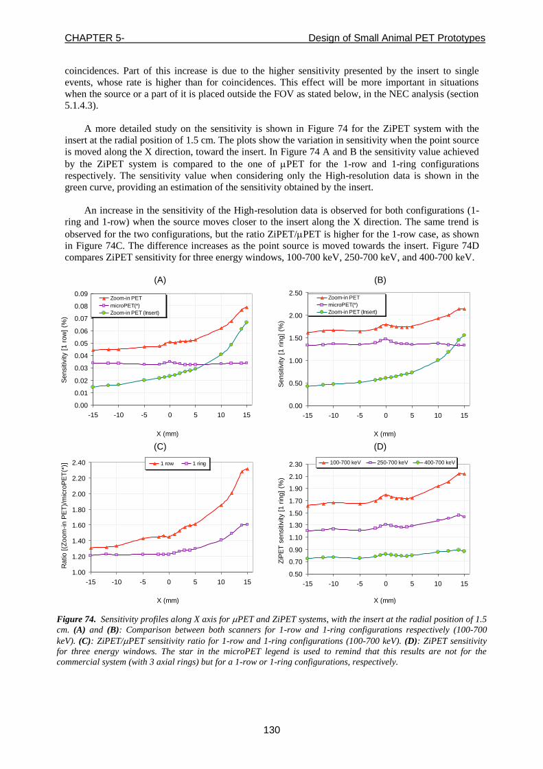
CHAPTER 5- Design of Small Animal PET Prototypes
130
coincidences. Part of this increase is due to the higher sensitivity presented by the insert to single
events, whose rate is higher than for coincidences. This effect will be more important in situations
when the source or a part of it is placed outside the FOV as stated below, in the NEC analysis (section
5.1.4.3).
A more detailed study on the sensitivity is shown in Figure 74 for the ZiPET system with the
insert at the radial position of 1.5 cm. The plots show the variation in sensitivity when the point source
is moved along the X direction, toward the insert. In Figure 74 A and B the sensitivity value achieved
by the ZiPET system is compared to the one of PET for the 1-row and 1-ring configurations
respectively. The sensitivity value when considering only the High-resolution data is shown in the
green curve, providing an estimation of the sensitivity obtained by the insert.
An increase in the sensitivity of the High-resolution data is observed for both configurations (1-
ring and 1-row) when the source moves closer to the insert along the X direction. The same trend is
observed for the two configurations, but the ratio ZiPET/PET is higher for the 1-row case, as shown
in Figure 74C. The difference increases as the point source is moved towards the insert. Figure 74D
compares ZiPET sensitivity for three energy windows, 100-700 keV, 250-700 keV, and 400-700 keV.
(A) (B)
0.00
0.01
0.02
0.03
0.04
0.05
0.06
0.07
0.08
0.09
-15 -10 -5 0 5 10 15
X (mm)
Sensitiv
ity [
1 r
ow
] (%
)
Zoom-in PET
microPET(*)
Zoom-in PET (Insert)
0.00
0.50
1.00
1.50
2.00
2.50
-15 -10 -5 0 5 10 15
X (mm)
Sensitiv
ity [
1 r
ing]
(%)
Zoom-in PET
microPET(*)
Zoom-in PET (Insert)
(C) (D)
1.00
1.20
1.40
1.60
1.80
2.00
2.20
2.40
-15 -10 -5 0 5 10 15
X (mm)
Ratio [
(Zoom
-in P
ET
)/m
icro
PE
T(*
)] 1 row 1 ring
0.50
0.70
0.90
1.10
1.30
1.50
1.70
1.90
2.10
2.30
-15 -10 -5 0 5 10 15
X (mm)
ZiP
ET
sensitiv
ity [
1 r
ing]
(%)
100-700 keV 250-700 keV 400-700 keV
Figure 74. Sensitivity profiles along X axis for PET and ZiPET systems, with the insert at the radial position of 1.5
cm. (A) and (B): Comparison between both scanners for 1-row and 1-ring configurations respectively (100-700
keV). (C): ZiPET/PET sensitivity ratio for 1-row and 1-ring configurations (100-700 keV). (D): ZiPET sensitivity
for three energy windows. The star in the microPET legend is used to remind that this results are not for the
commercial system (with 3 axial rings) but for a 1-row or 1-ring configurations, respectively.

CHAPTER 5- Design of Small Animal PET Prototypes
131
5.1.4.2. Depth of interaction (DOI)
Figure 75 shows the distribution of coincidences among effective layers for ZiPET with the insert
at the two radial positions (1.5 cm [left] and 3 cm [right]) with two PET blocks in coincidence with
the insert. Each set of 8 images for each configuration was independently normalized. The upper
images correspond to the coincidences between the insert and the opposite PET detector (block 15 in
the picture), while the lower images are for a more oblique combination (insert and the block 13). As
expected, the distribution of coincidences for the 1.5 cm radial position of the insert is more
concentrated around the central crystals because the insert in this case is closer to the point source.
Due to the asymmetric position of the center of the FOV with respect to the insert and the PET
detectors, the coincidences detected by each pair of detectors do not illuminate all the insert crystals.
An example of this is shown in Figure 76 for the ZiPET system with the insert placed at the radial
position of 3 cm. The figure analyzes the coincidences between the insert and the opposite PET
detector (block 15) and shows the distribution of coincidences for first and last effective layers. Note
that each image is normalized independently to show the distribution, but as it can be seen in Figure
75, the number of coincidences in the last layer is clearly lower than in the first one. Using geometric
relationships, the number of illuminated crystals (reddish area within green boundary in these figures)
can be easily computed. In addition to the predicted illuminated crystals, a surrounding area is
observed in the coincidences images (bluish region) due to scatter of gamma-rays in the crystal array.
It can be also seen that, for solid angle reasons, the number of illuminated crystals is higher for deeper
layers, being the scattered area larger as well.
r = 1.5 cm r = 3.0 cm
Figure 75. Distribution of coincidences for the ZiPET system with the insert at two radial positions (1.5 cm
[left] and 3 cm [right]) for two PET blocks in coincidence with the insert. The numbers on the insert
crystals arrays indicate the effective layer.
Quantitative results for the number of coincidences per effective layer for the system with the
insert in the radial position of 1.5 cm are shown in Figure 77 for three different energy windows. Data
from four PET blocks (see Figure 77A) in coincidence with the insert were evaluated (due to the
decrease in solid angle as the detectors move away from the front side of the insert, only these four
blocks and their symmetrical partners have a significant number of coincidences for an acquisition of a
centered point source). The plots were normalized dividing the number of coincidences in each layer
by the maximum number of coincidences in all the blocks studied, for each energy window. The
length of crystal representing the best tradeoff between resolution and sensitivity can be inferred from
the curves in Figure 77. For example, the number of coincidences for all the blocks (in the three
energy windows) detected by the two last layers is less than half the one detected in the layer with
more counts, suggesting that only minor sensitivity increase is provided by those layers, whereas they
degrade resolution and thus a shorter crystal can be used to enhance resolution with acceptable
degradation in sensitivity.

CHAPTER 5- Design of Small Animal PET Prototypes
132
Figure 76. Description of the experimental setup for the DOI analysis of the insert and microPET block 15 and
distribution of coincidences at the insert crystal array (64×64) for the first/last effective layers of the insert. The
radial position of the insert is 3 cm.
Due to the method used to determine the DOI (Z’) in the simulations (see section 5.1.3.2), and in
the real scanner (see section 5.1.1), the trend shown by the curves in Figure 77 slightly departs from
the theoretical law ze governing the absorption inside the crystal. This law predicts a maximum of
sensitivity at the first effective layer with an exponential drop in subsequent layers; however, as we
can see in Figure 77, the maximum of sensitivity is reached at the second effective layer for the
detectors closer to the front side of the insert (blocks 14 and 15). This result is an example of the
importance of using realistic simulation models of the system in order to take crucial decisions for
system design.
(A) (B)
(C) (D)
Figure 77. Coincidences per effective layer for the ZiPET system with the insert at the radial position of 1.5 cm for
three different energy windows.
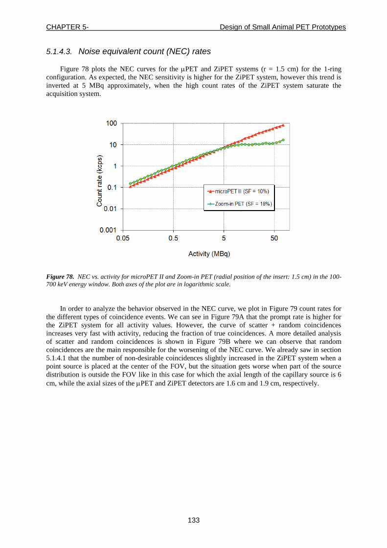
CHAPTER 5- Design of Small Animal PET Prototypes
133
5.1.4.3. Noise equivalent count (NEC) rates
Figure 78 plots the NEC curves for the PET and ZiPET systems (r = 1.5 cm) for the 1-ring
configuration. As expected, the NEC sensitivity is higher for the ZiPET system, however this trend is
inverted at 5 MBq approximately, when the high count rates of the ZiPET system saturate the
acquisition system.
Figure 78. NEC vs. activity for microPET II and Zoom-in PET (radial position of the insert: 1.5 cm) in the 100-
700 keV energy window. Both axes of the plot are in logarithmic scale.
In order to analyze the behavior observed in the NEC curve, we plot in Figure 79 count rates for
the different types of coincidence events. We can see in Figure 79A that the prompt rate is higher for
the ZiPET system for all activity values. However, the curve of scatter + random coincidences
increases very fast with activity, reducing the fraction of true coincidences. A more detailed analysis
of scatter and random coincidences is shown in Figure 79B where we can observe that random
coincidences are the main responsible for the worsening of the NEC curve. We already saw in section
5.1.4.1 that the number of non-desirable coincidences slightly increased in the ZiPET system when a
point source is placed at the center of the FOV, but the situation gets worse when part of the source
distribution is outside the FOV like in this case for which the axial length of the capillary source is 6
cm, while the axial sizes of the PET and ZiPET detectors are 1.6 cm and 1.9 cm, respectively.

CHAPTER 5- Design of Small Animal PET Prototypes
134
(A) (B)
Figure 79. Count rates vs. activity for microPET II and Zoom-inPET systems (radial position of the insert: 1.5
cm) in the 100-700 keV energy window for each type of coincidence event.
5.1.5. Conclusions
We have studied the ‘Zoom-in PET’ system, a high-resolution detector centered in the axial field
of view of the microPET II scanner with only one axial ring. The study has been performed using
Monte Carlo simulations with an extended version of PeneloPET. This extended version supports non-
standard geometries having two blocks of detectors at different radial positions, can deal with two
types of detectors with different features inside a single system and includes statistical blurring of the
depth of interaction distribution.
Since the spatial resolution was measured in previous works [Zhou and Qi, 2009, Qi et al., 2011]
proving its improvement, the performance evaluation of the system has been focused on sensitivity,
DOI capability of the insert and noise equivalent count rate. From the results we can state that there is
an evident improvement of sensitivity when the insert is included in the system. However, there is
room for improvement, given the fact that the current design with only one axial PET ring and the
size proposed for the insert does not provide optimal performance, since non-desirable coincidences,
such as pile-up, randoms, self-coincidences and scatter, increase very significantly when the insert is
present.
This section shows how simulations can guide the design of scanner prototypes, analyzing the
advantages and drawbacks before making final decisions. Our study suggest modifications in the
geometry of the system including, for example, more axial rings in the microPET II system and
shielding the insert from single events coming from outside the axial FOV.
CHAPTER 5- Design of Small Animal PET Prototypes
135
5.2. NIH PPI scanner
Many radionuclide molecular imaging studies do not, in practice, require tomographic images of
biological structures. In the early development of tumor-seeking agents, for example, it is common to
perform projection imaging studies in large groups of mice where the tumor can be grown at a location
favorable to projection imaging, e.g. the flank, and to observe the accumulation and elimination of the
agent from these tumors (and body) over extended periods of time, e.g. hours to tens of days. Since
many animals must be imaged many times, the imaging process must be as efficient as possible in
order to reduce the time needed to take the image to a minimum. Projection imaging of the tumor and
the whole body is an efficient way to provide these data: total tumor tracer content can be determined
with an accuracy that is not significantly different from tomographic measurements if the tumor is
located on the animal periphery, data processing time is reduced because image reconstruction is
eliminated and only a single region of interest is required to outline the tumor in each projection
image, etc. Importantly, projection imaging systems can be substantially less expensive than
tomographic systems of similar technology. All these reasons led to the design, assembly and test of
the positron projection imager (PPI) [Seidel et al., 2010].
The PPI system is a low cost bench top preclinical PET scanner dedicated to mouse studies. The
scanner employs compact dual-head geometry, similar to those of positron emission mammography
(PEM) systems [Murthy et al., 2000] or a high-sensitivity small-animal PET system based on High-
Resolution Research Tomograph detector technology [Kao et al., 2009]. The prototype system was
developed at the National Institutes of Health (NIH), Bethesda, MD (Molecular Imaging Program,
National Cancer Institute) where the author of this thesis was working on the summer 2011. It consists
of two large detectors placed facing each other with three possible face-to-face detector separations:
39, 29 and 19 mm. The system was specifically designed to work at a much lower radioactivity
concentration than current scanners, in order to reduce the dose delivered to mice, what is particularly
important in the case of longitudinal studies involving multiple PET procedures on the same animal.
In this work, PeneloPET Monte Carlo simulations were performed to provide a quantitative
analysis of system performance in terms of sensitivity, resolution and image quality. Although the
scanner was initially designed for projection imaging, in this work we explore the 3D imaging
potential of the system, analyzing spatial resolution and 3D image reconstruction possibilities. To this
end it was necessary to develop new methods of reconstruction adapting the existing algorithms to the
non-conventional geometry of the PPI system.
5.2.1. Setup description
The prototype consists of two opposed pixelated LYSO detector modules (Omega Piezo
Technology Inc., State College, PA) in time coincidence, mounted in a fixture that allows the face-to-
face separation between modules to be varied among 39, 29 and 19 mm (see Figure 80). The object to
be imaged is placed on a plastic plate located between the detectors faces such that the mid-plane of
the object can be made to coincide with the image plane which is always located exactly midway
between the detector faces. The detectors are kept stationary during the scan, making PPI a limited
angle tomography system. The FOV of the detectors is large enough to image the whole body of a
mouse in a single scan.
The individual LYSO crystals in each detector module are 1.51.512 mm3 with a pitch of 1.6
mm. Each crystal is polished on all sides and five of the sides are coated with a highly reflective
specular reflector. The exit surface of the 2659 array is covered by a 3.5 mm thick optical glass
window that is coupled with silicon grease to a pair of side-by-side Hamamatsu H8500C position-
sensitive photo-multiplier tubes (PSPMTs, Hamamatsu Corp., Bridgewater, NJ). These components
are shown in Figure 81. A 511 keV field flood image of this detector module is shown in Figure 82.

CHAPTER 5- Design of Small Animal PET Prototypes
136
Figure 80. Left: Conceptual drawing of the PPI. Right: picture of the prototype. It features a 64-channel DAQ
[Seidel et al., 2010].
The anodes of each H8500C PSPMT are combined by resistive division to yield eight row and
eight column signals for a total of 16 signals/PSPMT, 32 signals/module and 64 signals for the entire
system. These signals are acquired by a 64-channel data acquisition system (DAQ, Adaptive I/O
Technologies Inc., Blacksburg, VA) shown in Figure 80 (right). Digitization of these signals occurs if
the summed dynode signals of the two PSPMTs in one detector module are in time coincidence with
the summed dynode signals of the opposite module.
Figure 81. (A): disassembled PPI detector module; (B): assembled module with signal processing boards
attached [Seidel et al., 2010].

CHAPTER 5- Design of Small Animal PET Prototypes
137
Figure 82. 511 keV field flood image of the detector module shown in Figure 81. All 1534 individual crystals
can be identified [Seidel et al., 2010].
Table 33 reports the main PPI features employed in the simulations. Three different detector
separations: 39, 29 and 19 mm were simulated. To distinguish each configuration, we call them
PPI39mm, PPI29mm and PPI19mm, respectively.
Table 33. PPI parameters employed in the simulations.
parameter Value
general parameters coincidence time window 10 ns
iIntegration time 400 ns
coincidences dead-time 1200 ns
PPI detectors number of blocks per ring 2
number of blocks in coincidence 1
crystal array 2659
number of layers 1 (LYSO)
crystal size 1.51.512 mm3
reflector thickness 0.1 mm
energy resolution 14%
detector radius (separation between detectors)
39 mm / 29 mm / 19 mm
5.2.2. Image Reconstruction for the PPI
In order to characterize the system in terms of spatial resolution and image quality it is necessary
to reconstruct the PET data. Due to the non-conventional geometry of the PPI scanner, new methods
for image reconstruction had to be implemented [Vicente et al., 2012b].
5.2.2.1. Parallel imaging
As a first approximation, a parallel imaging algorithm was implemented. The projection image is
formed on the image plane midway between the two detector faces by backward projecting the counts
measured in the accepted LORs. Accepted LORs are those within a small, user-specified cone angle,
almost perpendicular to the image plane. Events occurring outside this cone angle are ignored. The
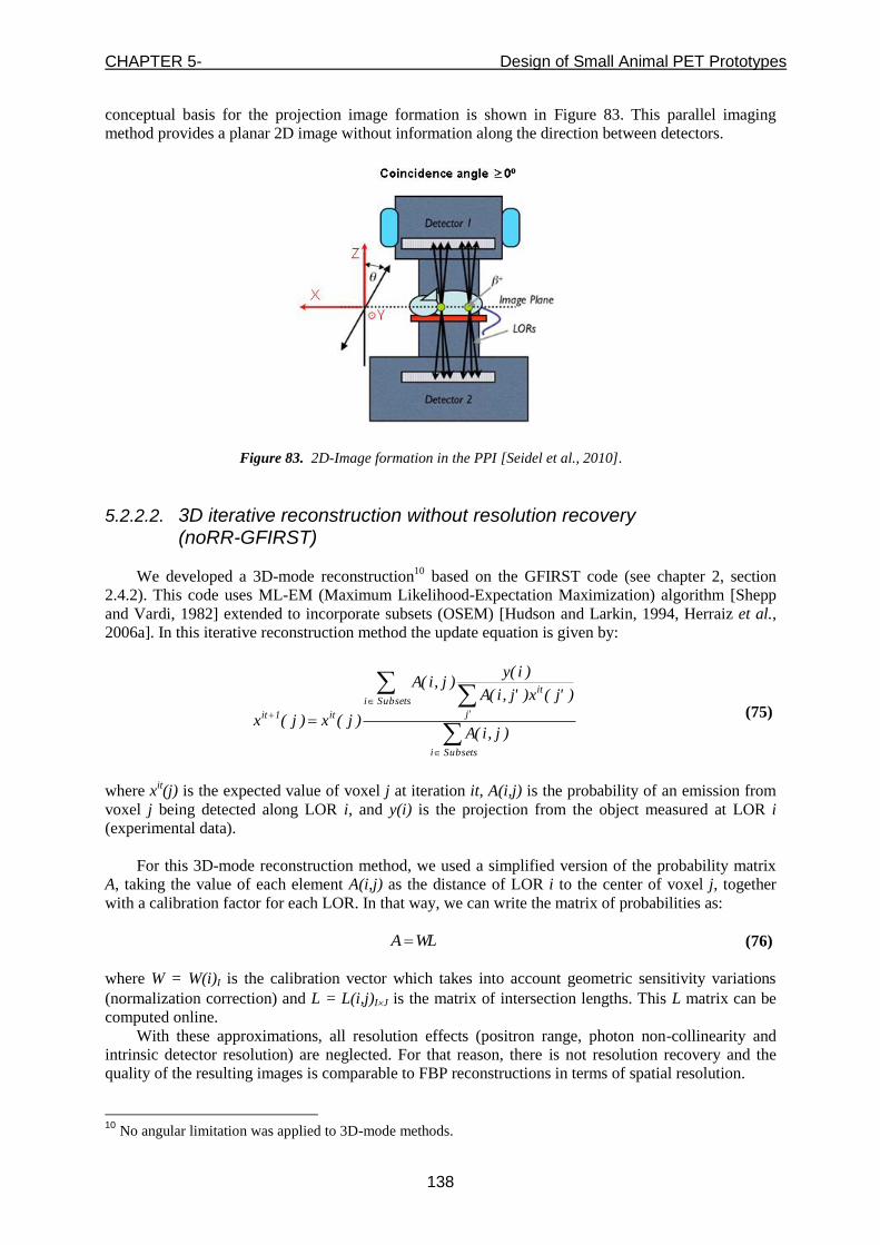
CHAPTER 5- Design of Small Animal PET Prototypes
138
conceptual basis for the projection image formation is shown in Figure 83. This parallel imaging
method provides a planar 2D image without information along the direction between detectors.
Figure 83. 2D-Image formation in the PPI [Seidel et al., 2010].
5.2.2.2. 3D iterative reconstruction without resolution recovery (noRR-GFIRST)
We developed a 3D-mode reconstruction10 based on the GFIRST code (see chapter 2, section
2.4.2). This code uses ML-EM (Maximum Likelihood-Expectation Maximization) algorithm [Shepp
and Vardi, 1982] extended to incorporate subsets (OSEM) [Hudson and Larkin, 1994, Herraiz et al.,
2006a]. In this iterative reconstruction method the update equation is given by:
Subsetsi
Subsetsi
'j
it
it1it
)j,i(A
)'j(x)'j,i(A
)i(y)j,i(A
)j(x)j(x (75)
where xit(j) is the expected value of voxel j at iteration it, A(i,j) is the probability of an emission from
voxel j being detected along LOR i, and y(i) is the projection from the object measured at LOR i
(experimental data).
For this 3D-mode reconstruction method, we used a simplified version of the probability matrix
A, taking the value of each element A(i,j) as the distance of LOR i to the center of voxel j, together
with a calibration factor for each LOR. In that way, we can write the matrix of probabilities as:
WLA (76)
where W = W(i)I is the calibration vector which takes into account geometric sensitivity variations
(normalization correction) and L = L(i,j)IJ is the matrix of intersection lengths. This L matrix can be
computed online.
With these approximations, all resolution effects (positron range, photon non-collinearity and
intrinsic detector resolution) are neglected. For that reason, there is not resolution recovery and the
quality of the resulting images is comparable to FBP reconstructions in terms of spatial resolution.
10
No angular limitation was applied to 3D-mode methods.
CHAPTER 5- Design of Small Animal PET Prototypes
139
5.2.2.3. 3D iterative reconstruction with resolution recovery (RR-GFIRST)
The second 3D-mode method implemented was also based on GFIRST code. In this method, we
used a more realistic probability matrix to account for resolution effects, which can be measured and
considered known. To this end, the matrix of probabilities A = A(i,j)IJ can be factorized as [Kupinski
and Barrett, 2005]:
WLHA (77)
The matrix H = H(j,j’)JJ accounts for finite resolution effects, L = L(i,j)IJ is the matrix of
intersection lengths, and W = W(i)I is the calibration vector as mentioned above. Then, the algorithm
becomes:
Subsetsi'j
Subsetsi
''j
it
'''j
'j
it1it
)'j,i(L)i(W)j,'j(H
)'''j(x)'''j,''j(H)''j,i(L
)i(y)'j,i(L)j,'j(H
)j(x)j(x (78)
The expression (78) can be rewritten in vector form:
itit1it csxx
(79)
where denotes an element-by-element multiplication of vectors, 1itx and itx
contain the new and
old image estimates, and s
contains the sensitivity correction factors of the denominator of eq. (78). itc
contains the multiplicative image correction values given by:
)xH(FP
yBPHc
itiSubseti
iTit
(80)
where FPi is an operator based on matrix L which forward projects vector itxH
along LOR i to give a
scalar value, and iBP is an operator which back projects a scalar value along LOR i into a 3D image
based on matrix L.
To simplify the computation in (80) and speed up the reconstruction, we consider the system as
shift-invariant. In this situation, the blurring component H can be taken as a shift-invariant kernel ρ
( ititTit xxHxH
). Then, the algorithm becomes:
)x(FP
yBPsxx
itiSubseti
iit1it
(81)
The kernel ρ can be defined as an effective point spread function (PSF) that takes into account the
aforementioned resolution effects. In order to obtain a realistic estimation of the kernel ρ, we used
point sources at different positions of the FOV and reconstructed the images using the 3D-mode
reconstruction method without resolution recovery explained above. From these images, the point
spread function (PSF) in the three directions was obtained. Since the PSF value is not shift-invariant in
this system, we selected a mean value of the PSF for each direction in order to apply the
approximation (81). We will investigate a non shift-invariant kernel in future works using the
algorithm form (80).
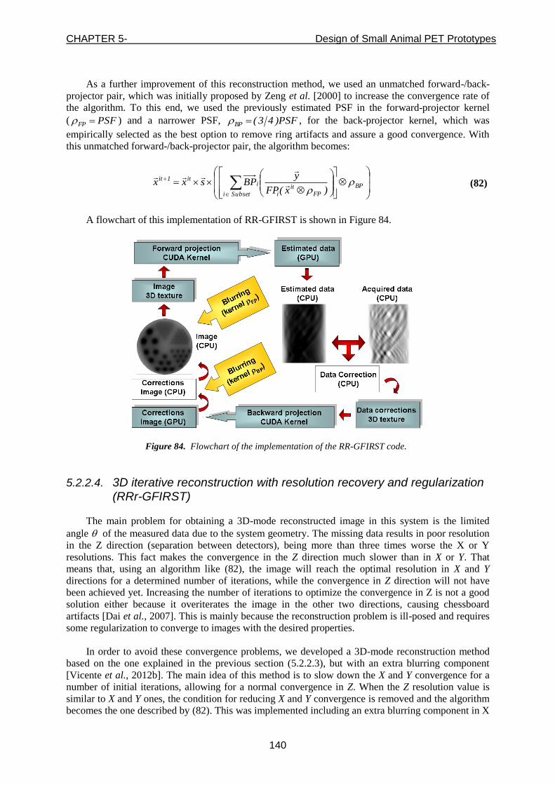
CHAPTER 5- Design of Small Animal PET Prototypes
140
As a further improvement of this reconstruction method, we used an unmatched forward-/back-
projector pair, which was initially proposed by Zeng et al. [2000] to increase the convergence rate of
the algorithm. To this end, we used the previously estimated PSF in the forward-projector kernel
( PSFFP ) and a narrower PSF, PSF)43(BP , for the back-projector kernel, which was
empirically selected as the best option to remove ring artifacts and assure a good convergence. With
this unmatched forward-/back-projector pair, the algorithm becomes:
BP
FPit
iSubseti
iit1it
)x(FP
yBPsxx
(82)
A flowchart of this implementation of RR-GFIRST is shown in Figure 84.
Figure 84. Flowchart of the implementation of the RR-GFIRST code.
5.2.2.4. 3D iterative reconstruction with resolution recovery and regularization (RRr-GFIRST)
The main problem for obtaining a 3D-mode reconstructed image in this system is the limited
angle of the measured data due to the system geometry. The missing data results in poor resolution
in the Z direction (separation between detectors), being more than three times worse the X or Y
resolutions. This fact makes the convergence in the Z direction much slower than in X or Y. That
means that, using an algorithm like (82), the image will reach the optimal resolution in X and Y
directions for a determined number of iterations, while the convergence in Z direction will not have
been achieved yet. Increasing the number of iterations to optimize the convergence in Z is not a good
solution either because it overiterates the image in the other two directions, causing chessboard
artifacts [Dai et al., 2007]. This is mainly because the reconstruction problem is ill-posed and requires
some regularization to converge to images with the desired properties.
In order to avoid these convergence problems, we developed a 3D-mode reconstruction method
based on the one explained in the previous section (5.2.2.3), but with an extra blurring component
[Vicente et al., 2012b]. The main idea of this method is to slow down the X and Y convergence for a
number of initial iterations, allowing for a normal convergence in Z. When the Z resolution value is
similar to X and Y ones, the condition for reducing X and Y convergence is removed and the algorithm
becomes the one described by (82). This was implemented including an extra blurring component in X

CHAPTER 5- Design of Small Animal PET Prototypes
141
and Y in the backprojector:
RNit
)Y,X(gReBP
FPit
iSubseti
iit1it
)x(FP
yBPsxx
(83)
where )Y,X(gRe is the additional blurring kernel for X and Y directions, N is the total number of
iterations and R is the number of the final iterations when the algorithm becomes the one described by
(82). Since the convolution of two Gaussians is another Gaussian, we can rewrite (83) with the kernel
BP in its X, Y and Z components as follows:
)Z(BP)Y(BP)X(BP
FPit
iSubseti
iit1it ,','
)x(FP
yBPsxx
(84)
where
N,RNitif'
RN,1itif'
)Y,X(BP)Y,X(BP
)Y,X(gRe)Y,X(BP)Y,X(BP
The selected kernel )Y,X(BP' , when it (N-R), is wider than the )XY(FP in order to control the
convergence of the image in each actualization. The value chosen for the kernel )Y,X(BP' .was
)Y,X(PSF3)Y,X('PSF
The value of the PSF of the kernel )Y,X(gRe and the number of iterations was selected based on
the difference in the convergence in Z direction compared to X and Y. These values were obtained after
several tests.
5.2.3. Simulated study of the performance of the scanner
We evaluated sensitivity and resolution in different positions within the FOV. Initial imaging
studies were also performed to demonstrate the imaging capabilities of the PPI system.
5.2.3.1. Sensitivity
The sensitivity of the system was measured at different positions within the FOV. For each
position we simulated a point source consisting of a sphere (0.2 mm diameter) of 18
F of 30 Ci in a
cubic phantom (111 cm3) of water, computing the number of detected coincidence over the actual
number of positron annihilations. The three detector distances explained above were evaluated in the
400-650 keV energy window. Additional measurements were performed for the separation of 39 mm
in two more energy windows (100-650 keV and 250-650 keV).
The point source simulations for each scanner configuration (i.e. distance between the detectors)
were variable depending of the FOV dimension in Z direction. The step of the point source shift was 2
mm in the three directions. A summary of the positions of the point sources for each configuration is
reported in Table 34.
CHAPTER 5- Design of Small Animal PET Prototypes
142
Table 34. Summary of the number of point source simulations performed for each system configuration (i.e.
separation between detectors) to get the 3D-sensitivity profiles.
Separation between detectors (mm)
# of X positions # of Y positions # of Z positions # of simulations
39 24 [0,46 mm] 10 [0,18 mm] 10 [0,18 mm] 2400
29 24 [0,46 mm] 10 [0,18 mm] 8 [0,14 mm] 1920
19 24 [0,46 mm] 10 [0,18 mm] 5 [0,8 mm] 1200
As we can see in the table, the number of point sources simulated for each configuration only
cover an eighth of the total FOV. The rest of the FOV was completed taking advantage of system
symmetries.
In order to validate the simulated results, the absolute central sensitivity (ACS) was also
measured experimentally using a point source similar to the one employed in the simulations.
5.2.3.2. Spatial resolution
To measure the spatial resolution of the system we simulated point sources (same size than in the
previous section) at different positions within the FOV. Each point source simulation was
reconstructed and activity profiles were drawn in the image in three directions and fitted to Gaussians
to calculate the FWHM. Since this system does not have cylindrical symmetry as standard PET
scanners, the resolution was measured along X, Y and Z directions. The resolution was evaluated for
the PPI system with the detectors separation of 39 mm (PPI39mm).
The image reconstruction was performed using two 3D-mode reconstruction methods: with and
without resolution recovery. The method without resolution recovery (noRR-GFIRST, section 5.2.2.2)
was employed to study what we call in this work ‘intrinsic resolution’. Intrinsic resolution in this
context means the system resolution without employing any resolution recovery procedure, as the FBP
algorithm, which is the standard reconstruction method employed to characterize the systems in term
of spatial resolution. We set the number of iterations to 5 as more than 5 iterations without including
resolution effects in the reconstruction produced Gibb’s artifacts. The method with resolution recovery
(RR-GFIRST, section 5.2.2.3) was used to explore the resolution limits of the system using a shift-
invariant kernel ρ, that is, the same PSF value for all the positions within the FOV. The number of
iterations was set to 200. It is straight forward to see that, since the resolution is measured using
isolated point sources, these measurements correspond to the maximum resolution achieved under
ideal conditions. Note that no regularization was applied in the recovery reconstruction method since
there is no problem with chessboard artifacts when reconstructing isolated point sources.
To evaluate the resolution, we first simulated a point source placed at the center of the FOV of the
PPI scanner including continuous rotation (4.5 degrees per second) of its detectors to provide a full
tomographic acquisition. Figure 85 shows a conceptual drawing of the PPI system with rotation. The
spatial resolution obtained with this system was compared with the one obtained with the standard
PPI39mm using the noRR-GFIRST method for the reconstruction.
Secondly, we studied the resolution variation within the FOV for the standard PPI39mm (without
rotation). To this end, we simulated point sources at different positions within the FOV. The step of
the point source shift was 4.5 mm in the three directions. A total of 176 simulations ({11 (X [0,40
mm])} {4 (Y [0,13 mm])} {4 (Z [0,13 mm])}) was performed covering approximately an
eighth of the total FOV. The rest of the FOV was completed taking advantage of system symmetries.
The resulting 3D profiles were used to evaluate the resolution along the 3 axes using both mentioned

CHAPTER 5- Design of Small Animal PET Prototypes
143
reconstruction methods.
Figure 85. Diagram of the PPI system with rotation. The dashed-lines represent different detector positions in
their continuous rotation movement (speed: 4.5 degrees per second)
Finally, we compared the resolution obtained from the simulations with the one measured in the
real system.
5.2.3.3. Initial imaging studies
Both simulated and real data were reconstructed. No corrections were applied to the data, except
normalization. Extra corrections will be included in future works. The system configuration chosen for
the imaging studies was the PPI39mm.
A conceptual drawing of the simulated acquisition performed is shown in Figure 86. A (3×3×3)
matrix of point sources was placed at the center of the FOV with a 7.5 mm separation between point
sources in the three directions. The acquired list-mode data were then histogrammed into a sinogram,
after applying an energy window of 100-650 keV. Images were reconstructed using noRR-GFIRST
and RR-GFIRST. The number of iterations without resolution recovery was set to 5 (to avoid Gibb’s
artifacts). Using resolution recovery the number of iterations could be set to 200.
Figure 86. Diagram of the (3×3×3) matrix of point sources.
An initial imaging study using experimental data was performed with a 20 g dead mouse bone
scan study. We chose a mouse bone scan since it is the biological acquisition most likely to clearly
show spatial variations of resolution over the imaging volume. The mouse was injected with 100 Ci
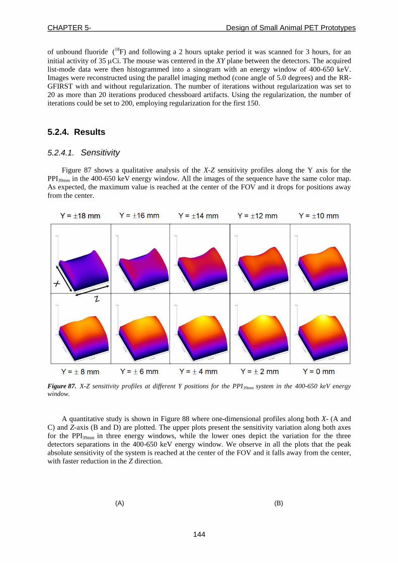
CHAPTER 5- Design of Small Animal PET Prototypes
144
of unbound fluoride (
18F) and following a 2 hours uptake period it was scanned for 3 hours, for an
initial activity of 35 Ci. The mouse was centered in the XY plane between the detectors. The acquired
list-mode data were then histogrammed into a sinogram with an energy window of 400-650 keV.
Images were reconstructed using the parallel imaging method (cone angle of 5.0 degrees) and the RR-
GFIRST with and without regularization. The number of iterations without regularization was set to
20 as more than 20 iterations produced chessboard artifacts. Using the regularization, the number of
iterations could be set to 200, employing regularization for the first 150.
5.2.4. Results
5.2.4.1. Sensitivity
Figure 87 shows a qualitative analysis of the X-Z sensitivity profiles along the Y axis for the
PPI39mm in the 400-650 keV energy window. All the images of the sequence have the same color map.
As expected, the maximum value is reached at the center of the FOV and it drops for positions away
from the center.
Figure 87. X-Z sensitivity profiles at different Y positions for the PPI39mm system in the 400-650 keV energy
window.
A quantitative study is shown in Figure 88 where one-dimensional profiles along both X- (A and
C) and Z-axis (B and D) are plotted. The upper plots present the sensitivity variation along both axes
for the PPI39mm in three energy windows, while the lower ones depict the variation for the three
detectors separations in the 400-650 keV energy window. We observe in all the plots that the peak
absolute sensitivity of the system is reached at the center of the FOV and it falls away from the center,
with faster reduction in the Z direction.
(A) (B)

CHAPTER 5- Design of Small Animal PET Prototypes
145
0
2
4
6
8
10
-50 -40 -30 -20 -10 0 10 20 30 40 50 60
X-axis (mm)
Se
nsitiv
ity (
%)
100-650 keV (3.9 cm) 250-650 keV (3.9 cm) 400-650 keV (3.9 cm)
0
2
4
6
8
10
-20 -15 -10 -5 0 5 10 15 20
Z-axis (mm)
Se
nsitiv
ity (
%)
100-650 keV (3.9 cm) 250-650 keV (3.9 cm) 400-650 keV (3.9 cm)
(C) (D)
0
2
4
6
8
10
-50 -40 -30 -20 -10 0 10 20 30 40 50 60
X-axis (mm)
Se
nsitiv
ity (
%)
400-650 keV (1.9 cm) 400-650 keV (2.9 cm) 400-650 keV (3.9 cm)
0
2
4
6
8
10
-20 -15 -10 -5 0 5 10 15 20
Z-axis (mm)
Se
nsitiv
ity (
%)
400-650 keV (1.9 cm) 400-650 keV (2.9 cm) 400-650 keV (3.9 cm)
Figure 88. One-dimensional sensitivity profiles along both X- (A and C) and Z-axis (B and D) for the PPI39mm
system in three energy windows (upper plots) and the three PPI configurations (i.e. detectors separation) in 400-
650 keV (lower plots).
Experimental values of the ACS are reported in Table 35 for the PPI39mm. We see a good
agreement between simulations and experimental values in both the 100-650 keV and 250-650 keV
energy windows with relative errors less than 5% and 8% respectively. However a high discrepancy is
observed for the sensitivity value obtained in the 400-700 keV energy window. This is most likely due
to energy calibration errors in the real scanner.
Table 35. Absolute central point sensitivity (ACS) comparison among different small animal PET scanners.
Results from simulations and experimental data are reported for the PPI39mm
System Reference Energy Window (keV) ACS (%)
PPI39mm (simulations)
---
100-650 9.5
250-650 7.2
400-650 6.2
PPI39mm (experimental
data) ---
100-650 10.0
250-650 6.7
400-650 4.5
PETbox [Zhang et al., 2011] 100-650 4.6
250-650 2.8
Argus
[Wang et al., 2006b]
(see chapter 3, section 3.1.2.1)
100-700 6.8
250-700 4.3
400-700 2.3
microPET P4 [Tai et al., 2001] 250-750 2.3
microPET R4 [Knoess et al., 2003] 250-750 4.4
Mosaic HP [Surti et al., 2005] 250-665 3.6
Inveon [Visser et al., 2009] 350-650 6.8
LabPET 12 [Bergeron et al., 2009] 250-650 5.4
From these results we can state that, due to the small distance between the detectors and its large

CHAPTER 5- Design of Small Animal PET Prototypes
146
size, the PPI system has a very competitive sensitivity value, improving the sensitivity of the PETbox
system [Zhang et al., 2011], a small animal PET scanner with similar characteristics (detector sensitive
area: 5×10 cm2, detectors separation: 5 cm) and improving most of the sensitivity values of full-ring
scanners. Table 35 reports an ACS comparison among several small animal PET scanners and the
simulated and experimental values for the PPI39mm system. .
5.2.4.2. Spatial resolution
Table 36. Spatial resolution at the center of the FOV for the PPI39mm without rotation vs. rotation. The point
sources images were reconstructed using the noRR-GFIRST method.
cFOV FWHM (mm)
X Y Z
Without rotation 1.2 1.2 5.4
With rotation 1.5 1.4 1.4
Table 36 shows a resolution comparison between the PPI39mm and the same system with rotation
as it was explained above. As commented, the incomplete LOR collection due to the system geometry
results in degradation in the Z resolution. System rotation recovers the missing data yielding very
similar resolution values in the three directions.
A more detailed study of the PPI39mm resolution (without rotation) is presented in Figure 89,
where resolution is plotted along the 3 axes for the reconstruction method without resolution recovery
(no RR, Figure 89A) and with resolution recovery (RR, Figure 89B). The study of the resolution
without resolution recovery shows the system intrinsic resolution with values mostly above 6 mm for
the Z direction and under 1.8 mm for the other two directions. These differences are reduced using the
PSF in the reconstruction. Although the Z resolution is still the worse value, in this case it is well
under 1.8 mm.
We compare in Table 37 the resolution measured in a point source placed at the center of the
FOV. It shows good agreement of simulations and experiment for both reconstruction methods. The
same good agreement is observed in Figure 90, where activity profiles along the Z direction are plotted
for the noRR-GFIRST (Figure 90A) and the RR-GFIRST (Figure 90B) methods. In Figure 90C we
also compare the experimental activity profile with and without resolution recovery, in order to see the
effect of including resolution effects.
(A) (B)

CHAPTER 5- Design of Small Animal PET Prototypes
147
0
1
2
3
4
5
6
7
8
9
-15 -10 -5 0 5 10 15
Z direction (mm)
Re
so
lutio
n (
mm
)
Z RESOLUTION (no RR) Y RESOLUTION (no RR) X RESOLUTION (no RR)
0
0.5
1
1.5
2
-15 -10 -5 0 5 10 15
Z direction (mm)
Re
so
lutio
n (
mm
)
Z RESOLUTION (RR) Y RESOLUTION (RR) X RESOLUTION (RR)
0
2
4
6
8
-50 -30 -10 10 30 50
X-axis (mm)
Re
so
lutio
n (
mm
)
0
0.5
1
1.5
2
-50 -30 -10 10 30 50
X-axis (mm)
Re
so
lutio
n (
mm
)
0
2
4
6
8
-15 -10 -5 0 5 10 15
Y-axis (mm)
Resolu
tion (
mm
)
0
0.5
1
1.5
2
-20 -10 0 10 20
Y-axis (mm)
Re
so
lutio
n (
mm
)
0
2
4
6
8
-15 -10 -5 0 5 10 15
Z-axis (mm)
Re
so
lutio
n (
mm
)
0
0.5
1
1.5
2
-15 -10 -5 0 5 10 15
Z-axis (mm)
Re
so
lutio
n (
mm
)
Figure 89. Resolution profiles along the 3 axes. Left (A, B and C): Reconstruction without resolution recovery (no
RR). Right (D, E and F): Reconstruction with resolution recovery (RR).
Table 37. Experimental vs. simulated resolution for a point source at the center of the FOV.
cFOV FWHM (mm)
X Y Z
No PSF Simulated data 1.2 1.2 5.4
Measured data 1.2 1.2 5.5
PSF info Simulated data 0.8 0.8 1.1
Measured data 0.9 0.8 1.2

CHAPTER 5- Design of Small Animal PET Prototypes
148
(A) (B) (C)
Figure 90. Experimental vs. simulated data comparison for a point source placed at the center of the FOV.
(A): Reconstruction without PSF information. (B): Reconstruction with PSF information
Finally, we compare in Table 38 resolution values at several Z positions (with X=0 and Y=0) for
the PPI39mm with the values reported in [Zhang et al., 2011] for the PETbox system. The PPI39mm
resolution values were obtained using the resolution recovery method (RR-GFIRST) since the PETbox
values were obtained using an iterative reconstruction method based on ML-EM algorithm with the
incorporation of a system probability matrix (P-matrix) [Bao et al., 2009b]. We observe that the
resolution of the PPI system is better in the three directions. This is because the individual crystal
elements of the PPI system have smaller cross-section size (PPI: 1.51.5 mm2, PETbox: 22 mm
2) and
the block detectors are closer in the PPI system (3.9 cm for the PPI vs 5 cm for the PETbox) resulting
in a less incomplete LOR collection in comparison with the PETbox.
Table 38. Spatial resolution at different Z positions (with X=0 and Y=0) for the PPI39mm and the PETbox
systems.
System Z position (mm) FWHM (mm) at (0,0,Z)
X Y Z
PPI39mm
(simulated data)
0 1.0 1.0 1.2
4.5 1.0 1.0 1.4
9 1.2 1.1 1.7
PETbox [Zhang et al., 2011]
0 1.6 1.5 2.6
6 1.5 1.4 2.7
5.2.4.3. Initial imaging studies
Figure 91 shows the reconstructed images from the initial simulated imaging study described in
Figure 86. The upper figures show three views of the image obtained without resolution recovery (left)
and with resolution recovery (right). We can observe how resolution is recovered in Z direction when
the shift-invariant blurring component, defined as an effective PSF, is included in the reconstruction.
This improvement in resolution can also be seen in the profile drawn along the Z direction (Figure 91,
down). However there remains room for improvement in the reconstruction method, for instance, we
can see that the point sources at the edges of the matrix in Y direction have less intensity than the
central ones and the regularization presented above did not improve the result.

CHAPTER 5- Design of Small Animal PET Prototypes
149
Figure 91. Reconstruction of a simulated (3×3×3) matrix of point sources for the PPI39mm configuration in the
100-650 keV energy window. Upper row shows the image reconstructed with the noRR-GFIRST code (left, 5
iterations) and the RR-GFIRST one (right, 200 iterations). Lower row shows an activity profile along Z axis as it
is marked (dashed lines) in the upper images.
Figure 92 shows a comparison of the parallel imaging method (cone angle of 5.0 degrees) and the
RR-GFIRST with and without regularization. The two 3D images were 2D-projected (average
intensity) in order to compare with the parallel imaging method. The first image in Figure 92 (left)
corresponds to the parallel imaging method, the next one (center) is the 3D reconstruction with
resolution recovery (20 iterations) and the third one is the 3D reconstruction with resolution recovery
and regularization (200 iterations, applying regularization in the first 150). We can observe that the
parallel imaging method is already a good estimation of the distribution of the 18
F in the mouse. The
3D methods get better results largely improving the resolution, even allowing distinguishing small
structures as, for example, ribs, bowels and the peculiar shape of the mouse elbow. An evident
improvement in image quality for the reconstruction (right) with regularization is also observed.
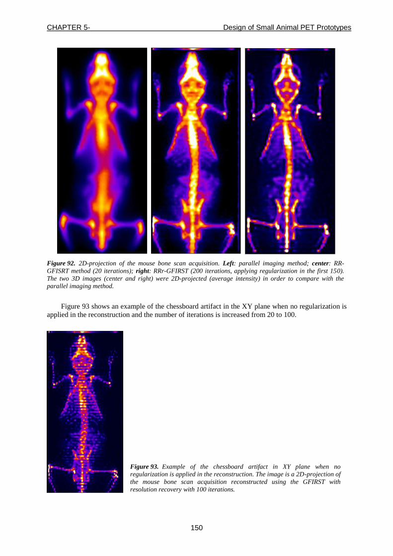
CHAPTER 5- Design of Small Animal PET Prototypes
150
Figure 92. 2D-projection of the mouse bone scan acquisition. Left: parallel imaging method; center: RR-
GFISRT method (20 iterations); right: RRr-GFIRST (200 iterations, applying regularization in the first 150).
The two 3D images (center and right) were 2D-projected (average intensity) in order to compare with the
parallel imaging method.
Figure 93 shows an example of the chessboard artifact in the XY plane when no regularization is
applied in the reconstruction and the number of iterations is increased from 20 to 100.
Figure 93. Example of the chessboard artifact in XY plane when no
regularization is applied in the reconstruction. The image is a 2D-projection of
the mouse bone scan acquisition reconstructed using the GFIRST with
resolution recovery with 100 iterations.

CHAPTER 5- Design of Small Animal PET Prototypes
151
However the interesting improvement here is in Z direction. In order to show the resolution
increase when regularization is applied to control convergence in the XY plane, we present in Figure
94 and Figure 95 an image sequence of a volume render for each reconstruction method (without and
with regularization respectively). The image sequence is a set of 18 images of a 180º rotation of the
mouse.
Figure 94. Image sequence of a volume render of the mouse bone scan reconstructed with the RR-GFIRST. The
sequence is a set of 18 images showing the 180º rotation of the mouse. The number of iterations was set to 20 in
order to avoid chessboard artifacts in the XY plane.

CHAPTER 5- Design of Small Animal PET Prototypes
152
Figure 94 (3D reconstruction without regularization) shows a good estimation of the 18
F activity
in the mouse for XY plane, which is deteriorated in Z direction with resolutions more than double the
XY ones. Regularization, as it was explained in section 5.2.2.4, allows to increase the number of
iterations from 20 (Figure 94) to 200 (Figure 95), controlling the convergence in XY in the first 150.
The resulting image has still better resolution in XY plane than in Z direction, but the Z resolution
improves vastly.
Figure 95. Image sequence of a volume render of the mouse bone scan reconstructed with the RRr-GFIRST.
The sequence is a set of 18 images showing the 180º rotation of the mouse. The number of iterations was set to
200, applying regularization in X and Y directions in the first 150.

CHAPTER 5- Design of Small Animal PET Prototypes
153
5.2.5. Conclusions
The PPI system was designed as low cost option for studies in mice. Compared with
commercially available small animal PET scanners, the bench top configuration of this system greatly
reduces the cost as well as the space needed for researchers to access PET imaging technology. While
a very high performance scanner was not the goal of the PPI design, the key performance metrics for
the system were chosen to satisfy typical resolution and sensitivity requirements. This section
demonstrates that the prototype system meets the design specifications.
Due to the dual-head geometry, the PPI system provides a limited angle tomography along the
direction between detectors (Z direction). Image reconstruction for such geometry depends on the
accurate system modeling [Moses and Qi, 2003]. In this work, different approaches and new
reconstruction methods has been implemented from a parallel imaging method which provides planar
2D images without information of the Z direction, to more accurate 3D-mode reconstructions based on
GFIRST [Herraiz et al., 2011] with three different approximations. In the first one, we used a
simplified version of the probability matrix, disregarding resolution effects. This method was
employed to measure the spatial resolution of the system since the quality of the resulting images is
comparable, in terms of spatial resolution, to a FBP reconstruction, the standard reconstruction method
to measure the spatial resolution in PET scanners. In the second 3D-mode method, we included
resolution effects by means of a shift-invariant blurring component defined as an effective point
spread function (PSF) and an unmatched forward-/back-projector pair to increase the convergence rate
of the algorithm. Finally, a novel method was implemented, improving the latter method with an extra
blurring component to regularize the convergence in X and Y directions.
This work has shown that the PPI system has very competitive sensitivities values, being some
experimental ACS values, for example: 10% at 100-650 keV, 7% at 250-650 keV and 5% at 400-650
keV. These results improve the sensitivity of the PETbox system [Zhang et al., 2010, Zhang et al.,
2011], being the PPI sensitivity at 400-650 keV window about the same as the PETbox at 100-650
keV window. The PPI system also improves most of the sensitivity values of full-ring scanners.
Regarding to the resolution measurements, the system has high resolution in the XY plane with values
less than 1.8 mm and practically uniform in all the FOV (which can fits a whole body mouse).
However, the incomplete LOR collection due to the system geometry results in degradation of the Z
resolution, with values mostly above 6 mm when no resolution recovery is applied in the
reconstruction. These differences are reduced using PSF information in the reconstruction. Then the Z
resolution is still the worse value, but reasonably under 1.8 mm in Z direction and under 1.4 mm in the
other two directions.
Finally, the initial images showed in this work, using the aforementioned reconstruction methods,
have demonstrated the imaging capabilities of the PPI system and the potential of the novel
reconstruction method with regularization.

CHAPTER 5- Design of Small Animal PET Prototypes
154
5.3. References Agostinelli, S. 2003. GEANT4 - a simulation toolkit. Nucl. Inst. Meth. In Phy. Res. A, 506, 250-303.
Bao, Q., Newport, D., Chen, M., Stout, D. B. & Chatziioannou, A. F. 2009a. Performance evaluation of the inveon
dedicated PET preclinical tomograph based on the NEMA NU-4 standards. J Nucl Med, 50, 401-8.
Bao, Q., Rannou, F. R., Taschereau, R., Stout, D. B. & Chatziioannou, A. F. 2009b. Image reconstruction for PETbox, a
benchtop preclinical PET tomograph. In: Nuclear Science Symposium Conference Record (NSS/MIC), 2009
IEEE, Oct. 24 2009-Nov. 1 2009 2009b. 2733-2737.
Baró, J., Sempau, J., Fernández-Varea, J. M. & Salvat, F. 1995. PENELOPE: An algorithm for Monte Carlo simulation of
the penetration and energy loss of electrons and positrons in matter. Nucl. Inst. Meth. In Phy. Res. B, 100, 31-46.
Bergeron, M., Cadorette, J., Bureau-Oxton, C., Beaudoin, J. F., Tetrault, M. A., Leroux, J. D., Lepage, M. D., Robert, G.,
Fontaine, R. & Lecomte, R. 2009. Performance evaluation of the LabPET12, a large axial FOV APD-based
digital PET scanner. In: Nuclear Science Symposium Conference Record (NSS/MIC), 2009 IEEE, Oct. 24 2009-
Nov. 1 2009 2009. 4017-4021.
Briesmeister, J. F. 1993. MNCP 4 A, Monte Carlo N-Particle Transport System. Los Alamos, New Mexico: Los Alamos
National Laboratory.
Clinthorne, N. H., Sangjune, P., Rogers, W. L. & Ping-Chun, C. 2003. Multi-resolution image reconstruction for a high-
resolution small animal PET device. In: Nuclear Science Symposium Conference Record, 2003 IEEE, 19-25
Oct. 2003 2003. 1997-2001 Vol.3.
Chatziioannou, A. F. 2002. PET scanners dedicated to molecular imaging of small animal models. Mol Imaging Biol, 4, 47-
63.
Dai, S., Han, M., Xu, W., Wu, Y. & Gong, Y. 2007. Soft Edge Smoothness Prior for Alpha Channel Super Resolution. In:
Computer Vision and Pattern Recognition, 2007. CVPR '07. IEEE Conference on, 17-22 June 2007 2007. 1-8.
España, S., Herraiz, J. L., Vicente, E., Vaquero, J. J., Desco, M. & Udias, J. M. 2009. PeneloPET, a Monte Carlo PET
simulation tool based on PENELOPE: features and validation. Phys Med Biol, 54, 1723-42.
Harrison, R. L., Vannoy, S. D., Haynor, D. R., Gillispie, S. B., Kaplan, M. S. & Lewellen, T. K. 1993. Preliminary
Experience With The Photon History Generator Module Of A Public-domain Simulation System For Emission
Tomography. In: Nuclear Science Symposium and Medical Imaging Conference, 1993., 1993 IEEE Conference
Record., 31 Oct-6 Nov 1993 1993. 1154-1158.
Heinrichs, U., Pietrzyk, U. & Ziemons, K. 2003. Design optimization of the PMT-ClearPET prototypes based on
simulation studies with GEANT3. Nuclear Science, IEEE Transactions on, 50, 1428-1432.
Herraiz, J. L., Espana, S., Vaquero, J. J., Desco, M. & Udias, J. M. 2006a. FIRST: Fast Iterative Reconstruction Software
for (PET) tomography. Phys Med Biol, 51, 4547-65.
Herraiz, J. L., España, S., Cabido, R., Montemayor, A. S., Desco, M., Vaquero, J. J. & Udias, J. M. 2011. GPU-Based Fast
Iterative Reconstruction of Fully 3-D PET Sinograms. Nuclear Science, IEEE Transactions on, 58, 2257-2263.
Hudson, H. M. & Larkin, R. S. 1994. Accelerated image reconstruction using ordered subsets of projection data. Medical
Imaging, IEEE Transactions on, 13, 601-609.
Huh, S. S., Rogers, W. L. & Clinthorne, N. H. 2008. On-line sliding-window list-mode PET image reconstruction for a
surgical pet imaging probe. In: Nuclear Science Symposium Conference Record, 2008. NSS '08. IEEE, 19-25
Oct. 2008 2008. 5479-5484.
James, S. S., Yang, Y., Wu, Y., Farrell, R., Dokhale, P., Shah, K. S. & Cherry, S. R. 2009. Experimental characterization
and system simulations of depth of interaction PET detectors using 0.5 mm and 0.7 mm LSO arrays. Phys Med
Biol, 54, 4605-19.
Jan, S., Santin, G., Strul, D., Staelens, S., Assie, K., Autret, D., Avner, S., Barbier, R., Bardies, M., Bloomfield, P. M.,
Brasse, D., Breton, V., Bruyndonckx, P., Buvat, I., Chatziioannou, A. F., Choi, Y., Chung, Y. H., Comtat, C.,
Donnarieix, D., Ferrer, L., Glick, S. J., Groiselle, C. J., Guez, D., Honore, P. F., Kerhoas-Cavata, S., Kirov, A. S.,
Kohli, V., Koole, M., Krieguer, M., van der Laan, D. J., Lamare, F., Largeron, G., Lartizien, C., Lazaro, D.,
Maas, M. C., Maigne, L., Mayet, F., Melot, F., Merheb, C., Pennacchio, E., Perez, J., Pietrzyk, U., Rannou, F. R.,
Rey, M., Schaart, D. R., Schmidtlein, C. R., Simon, L., Song, T. Y., Vieira, J. M., Visvikis, D., Van de Walle, R.,
Wieers, E. & Morel, C. 2004b. GATE: a simulation toolkit for PET and SPECT. Phys Med Biol, 49, 4543-61.
Janecek, M., Heyu, W. & Yuan-Chuan, T. 2006. A simulation study for the design of a prototype insert for whole-body
PET scanners. Nuclear Science, IEEE Transactions on, 53, 1143-1149.
Kao, C.-M., Xie, Q., Dong, Y., Wan, L. & Chen, C.-T. 2009. A High-Sensitivity Small-Animal PET Scanner:
Development and Initial Performance Measurements. Nuclear Science, IEEE Transactions on, 56, 2678-2688.
Keesing, D. B., Pal, D., O'Sullivan, J. A., Komarov, S., Wu, H. & Tai, Y.-C. 2008. System modeling of a DOI-capable
half-ring PET insert device for breast cancer imaging. In: Nuclear Science Symposium Conference Record,
CHAPTER 5- Design of Small Animal PET Prototypes
155
2008. NSS '08. IEEE, 19-25 Oct. 2008 2008. 4218-4222.
Knoess, C., Siegel, S., Smith, A., Newport, D., Richerzhagen, N., Winkeler, A., Jacobs, A., Goble, R. N., Graf, R.,
Wienhard, K. & Heiss, W. D. 2003. Performance evaluation of the microPET R4 PET scanner for rodents. Eur J
Nucl Med Mol Imaging, 30, 737-47.
Kupinski, M. A. & Barrett, H. H. 2005. Small-animal Spect Imaging, Springer.
Miyaoka, R. S., Janes, M. L., Lee, K., Park, B., Kinahan, P. E. & Lewellen, T. K. 2005. Development of a single detector
ring micro crystal element scanner: QuickPET II. Mol Imaging, 4, 117-27.
Moses, W. W. & Qi, J. 2003. Fundamental limits of positron emission mammography. Nuclear Instruments and Methods
in Physics Research Section A: Accelerators, Spectrometers, Detectors and Associated Equipment, 497, 82-89.
Park, S. J., Rogers, W. L. & Clinthorne, N. H. 2007. Design of a very high-resolution small animal PET scanner using a
silicon scatter detector insert. Phys Med Biol, 52, 4653-77.
Pavlopoulos, S. & Tzanakos, G. 1993. Design and performance evaluation of a high resolution small animal positron
tomograph. In: Nuclear Science Symposium and Medical Imaging Conference, 1993., 1993 IEEE Conference
Record., 31 Oct-6 Nov 1993 1993. 1697-1701 vol.3.
Pavlopoulos, S. & Tzanakos, G. 1996. Design and performance evaluation of a high-resolution small animal positron
tomograph. Nuclear Science, IEEE Transactions on, 43, 3249-3255.
Qi, J., Yang, Y., Zhou, J., Wu, Y. & Cherry, S., R. 2011. Experimental assessment of resolution improvement of a zoom-in
PET. Physics in Medicine and Biology, 56, N165.
Rogers, D. W. O. 1984. Low energy electron transport with EGS. Nucl. Inst. Meth. In Phy. Res. A, 227, 535-48.
Rouze, N. C., Schmand, M., Siegel, S. & Hutchins, G. D. 2004. Design of a small animal PET imaging system with 1
microliter volume resolution. Nuclear Science, IEEE Transactions on, 51, 757-763.
Seidel, J., Wenze, X., Kakareka, J. W., Pohida, T. J., Green, M. V. & Choyke, P. L. 2010. A positron projection imager for
whole-body mouse imaging. In: Nuclear Science Symposium Conference Record (NSS/MIC), 2010 IEEE, Oct.
30 2010-Nov. 6 2010 2010. 2206-2209.
Shepp, L. A. & Vardi, Y. 1982. Maximum Likelihood Reconstruction for Emission Tomography. Medical Imaging, IEEE
Transactions on, 1, 113-122.
Stickel, J. R. & Cherry, S. R. 2005. High-resolution PET detector design: modelling components of intrinsic spatial
resolution. Phys Med Biol, 50, 179-95.
Tai, C., Chatziioannou, A., Siegel, S., Young, J., Newport, D., Goble, R. N., Nutt, R. E. & Cherry, S. R. 2001. Performance
evaluation of the microPET P4: a PET system dedicated to animal imaging. Phys Med Biol, 46, 1845-62.
Tai, Y. C., Chatziioannou, A. F., Yang, Y., Silverman, R. W., Meadors, K., Siegel, S., Newport, D. F., Stickel, J. R. &
Cherry, S. R. 2003. MicroPET II: design, development and initial performance of an improved microPET scanner
for small-animal imaging. Phys Med Biol, 48, 1519-37.
Tai, Y. C., Wu, H., Pal, D. & O'Sullivan, J. A. 2008. Virtual-pinhole PET. J Nucl Med, 49, 471-9.
Thompson, C. J., Moreno-Cantu, J. & Picard, Y. 1992a. PETSIM: Monte Carlo simulation of all sensitivity and resolution
parameters of cylindrical positron imaging systems. Physics in Medicine and Biology, 37, 731.
Thompson, C. J., Moreno-Cantu, J. & Picard, Y. 1992b. PETSIM: Monte Carlo simulation of all sensitivity and resolution
parameters of cylindrical positron imaging systems. Phys Med Biol, 37, 731-49.
Tzanakos, G. & Pavlopoulos, S. 1991. Modeling and simulation of a PET scanner. In: Nuclear Science Symposium and
Medical Imaging Conference, 1991., Conference Record of the 1991 IEEE, 2-9 Nov. 1991 1991. 1689-1694
vol.3.
Tzanakos, G. & Pavlopoulos, S. 1993. Design and performance evaluation of a new high resolution detector array module
for PET. In: Nuclear Science Symposium and Medical Imaging Conference, 1993., 1993 IEEE Conference
Record., 31 Oct-6 Nov 1993 1993. 1842-1846 vol.3.
Urosevic, J., Sauzeau, V., Soto-Montenegro, M. L., Reig, S., Desco, M., Burkitt Wright, E. M., Cañamero, M., Mulero, F.,
Ortega, S., Bustelo, X. R. & Barbacid, M. 2011. Constitutive activation of B-Raf in the mouse germ line provides
a model for human cardio-facio-cutaneous syndrome. P Natl Acad Sci USA, 108, 5015-5020.
Vicente, E., Herraiz, J. L., Seidel, J., Green, M. V., Desco, M., Vaquero, J. J. & Udias, J. M. 2012b. Regularization of 3D
Iterative Reconstruction for a Limited-Angle PET Tomograph. In: Nuclear Science Symposium Conference
Record (NSS/MIC), 2012 IEEE (Accepted), 2012b.
Visser, E. P., Disselhorst, J. A., Brom, M., Laverman, P., Gotthardt, M., Oyen, W. J. & Boerman, O. C. 2009. Spatial
resolution and sensitivity of the Inveon small-animal PET scanner. J Nucl Med, 50, 139-47.
Wang, Y., Seidel, J., Tsui, B. M., Vaquero, J. J. & Pomper, M. G. 2006b. Performance evaluation of the GE healthcare
eXplore VISTA dual-ring small-animal PET scanner. J Nucl Med, 47, 1891-900.
Watanabe, M., Uchida, H., Okada, H., Shimizu, K., Satoh, N., Yoshikawa, E., Ohmura, T., Yamashita, T. & Tanaka, E.
1992. A high resolution PET for animal studies. Medical Imaging, IEEE Transactions on, 11, 577-580.
Wu, H., Pal, D., O'Sullivan, J. A. & Tai, Y. C. 2008a. A feasibility study of a prototype PET insert device to convert a
general-purpose animal PET scanner to higher resolution. J Nucl Med, 49, 79-87.

CHAPTER 5- Design of Small Animal PET Prototypes
156
Wu, H., Pal, D., Song, T. Y., O'Sullivan, J. A. & Tai, Y. C. 2008b. Micro insert: a prototype full-ring PET device for
improving the image resolution of a small-animal PET scanner. J Nucl Med, 49, 1668-76.
Wu, H., Song, T. Y., Pal, D., Keesing, D. B., Komarov, S., O Sullivan, J. A. & Tai, Y.-C. 2008c. A high resolution PET
insert system for clinical PET/CT scanners. In: Nuclear Science Symposium Conference Record, 2008. NSS '08.
IEEE, 19-25 Oct. 2008 2008c. 5442-5444.
Yang, Y., Dokhale, P. A., Silverman, R. W., Shah, K. S., McClish, M. A., Farrell, R., Entine, G. & Cherry, S. R. 2006.
Depth of interaction resolution measurements for a high resolution PET detector using position sensitive
avalanche photodiodes. Phys Med Biol, 51, 2131-42.
Yang, Y., Tai, Y. C., Siegel, S., Newport, D. F., Bai, B., Li, Q., Leahy, R. M. & Cherry, S. R. 2004. Optimization and
performance evaluation of the microPET II scanner for in vivo small-animal imaging. Phys Med Biol, 49, 2527-
45.
Zaidi, H. & Scheurer, C. 1999. An object-oriented Monte Carlo simulator for 3D cylindrical positron tomographs. Comput.
Methods Programs Biomed., 58, 133-45.
Zeng, G. L. & Gullberg, G. T. 2000. Unmatched projector/backprojector pairs in an iterative reconstruction algorithm.
Medical Imaging, IEEE Transactions on, 19, 548-555.
Zhang, H., Bao, Q., Vu, N. T., Silverman, R. W., Taschereau, R., Berry-Pusey, B. N., Douraghy, A., Rannou, F. R., Stout,
D. B. & Chatziioannou, A. F. 2011. Performance evaluation of PETbox: a low cost bench top preclinical PET
scanner. Mol Imaging Biol, 13, 949-61.
Zhou, J. & Qi, J. 2009. Theoretical analysis and simulation study of a high-resolution zoom-in PET system. Physics in
Medicine and Biology, 54, 5193.
Zhou, J. & Qi, J. 2010. Efficient system modeling of a high-resolution zoom-in PET scanner. In: Nuclear Science
Symposium Conference Record (NSS/MIC), 2010 IEEE, Oct. 30 2010-Nov. 6 2010 2010. 3501-3505.
Zhou, J. & Qi, J. 2011. Adaptive Imaging for Lesion Detection Using a Zoom-in PET System. Medical Imaging, IEEE
Transactions on, 30, 119-130.
Conclusions of this Thesis
157
Conclusions of this Thesis
Small-animal PET is a complex technique, which has gained increasing impact in recent years
due to the development of dedicated systems. There remain many challenges regarding
instrumentation, data evaluation and experimentation, which need to be overcome in order to achieve
reliable and valuable small animal PET data.
This thesis has presented original contributions to the study of the sources of error that limit the
quality of PET images providing new methods and algorithms to compensate them, and improvements
in Monte Carlo simulations and existing reconstruction codes to extend them to the non-conventional
geometry of new modern designs.
The main contributions of this thesis are:
1. A detailed performance evaluation of two dedicated small-animal scanners with very different
geometries and features, the SEDECAL rPET and the SEDECAL Argus systems, showing the
importance of standardized protocols to assess the performance. A critical comparison between
these two scanners and to other preclinical PET systems available on the market has been also
briefly presented, showing that both scanners have very competitive features improving in some
parameters the performance of other commercial systems.
2. It has also been shown that the protocols to assess the scanner performance are not flawless,
analyzing in detail some examples and, with the help of very detailed and realistic simulations,
we have proposed improvements on some procedures. An example of these proposals is a way
to upgrade the NEMA protocol to measure scatter fraction to make it isotope range-independent.
This extension to the NEMA protocol includes a deconvolution of the radial sinogram profiles
using a one-dimensional distribution of the positron range in order to remove range effects from
sinogram profiles. The improved protocol has been tested for 68
Ga, a radionuclide with large
positron range, yielding the same results than using 18
F, the isotope proposed by NEMA.
3. From the limitations observed in the scanners evaluated, new correction methods and algorithms
have been developed. They are relevant not only for these particular scanners, but easily
adaptable to different architectures provided they comply with certain common design
constraints. Namely:
3.1. A new method to linearize the total count rates getting rid of non linear effects due to dead-
time losses and pile-up losses and gains within the selected energy window. The method is
based on the linear relationship between the effective dead-time (which takes into account
dead-time and pile-up effects) , and the Singles-to-Coincidences ratio (SCR). Results have
shown that, using the proposed method, corrected count rates are accurate within 7%, even
when high activities are present in the FOV, avoiding the bias that appears when using a
single-parameter procedure. We have verified the method using experimental and
simulated data from rPET and Argus systems, demonstrating its applicability.
3.2. A novel calibration protocol developed and implemented in a software tool, to compensate
the effect of small mechanical misalignments in rotating PET systems with planar
detectors. This calibration tool determines the misalignments within acceptable tolerance in
each geometrical parameter. The results highlight the importance of the characterization of
detector misalignment whose effect, if they are not properly corrected, may result in loss of
resolution and artifacts with severe degradation of the reconstructed image.
3.3. An attenuation correction based on Computed Tomography (CT) images. PET images

Conclusions of this Thesis
158
corrected with the tool presented in this thesis have demonstrated to exhibit better
quantification and more consistency between the reconstructed image and the acquired data
than the ones obtained with simpler methods, as for example an attenuation correction
based on a FOV-sized water cylinder.
4. Making use of all the experience gained during the characterization of the scanners and the study
of the sources of error that limit the quality of the images, Monte Carlo simulation tools have been
developed and extended to guide in the design of new prototypes, performing as well the
necessary modifications in the available reconstruction methods to adapt the existing codes to the
non-conventional geometry of the new designs. Two different new designs have been studied:
4.1. Zoom-in PET scanner: a high-resolution detector centered in the axial field of view of the
microPET II scanner with only one axial ring. Monte Carlo simulation studies were
performed with a modified version of the PeneloPET package. This modification was
required in order to support the non-standard geometrical configuration of this scanner.
This study is an example of how simulated data can help to guide the design of new
prototypes, analyzing all the advantages and drawbacks before taking the final decision on
the construction. The results obtained suggested to modify the geometry of the system, for
example, by adding more axial rings to the microPET II system and further trying to shield
the insert to avoid single events from outside the axial FOV to reach the insert.
4.2. NIH PPI: a low-cost high-sensitivity bench-top preclinical PET system consisting of a
compact dual stationary head geometry. This system is a limited angle tomography system,
with very poor sampling in the direction perpendicular to the detectors. Due to this poor
sampling in one direction, it has been necessary to develop new approaches for the
reconstruction, such as a new regularization procedure for a 3D reconstruction algorithm
which employs variable, direction-dependent filtering between iterations, allowing for the
convergence speed to be more isotropic. The performance evaluation presented has
demonstrated that the prototype system meets the intended design specifications. The initial
images have shown the imaging capabilities of the PPI system and the potential of the
novel reconstruction method with regularization.
As a summarizing conclusion, this thesis shows the power of detailed MC simulations in the
improvement of existing scanners and performance assessment protocols and in the design of new
scanners.
The results described in conclusions 3.2 and 3.3 have been transferred to the industry and an
implementation is integrated on the small-animal, high-resolution molecular imaging systems
manufactured by SEDECAL (Madrid, Spain) and distributed world-wide.

Publications Derived from this Thesis
159
Publications Derived from this Thesis
Papers Published in International Journals
1. A. L. Goertzen, Q. Bao, M. Bergeron, E. Blankemeyer, S. Blinder, M. Cañadas, A. F.
Chatziioannou, K. Dinelle, E. Elhami, H.-S. Jans, E. Lage, R. Lecomte, V. Sossi, S. Surti, Y.-
C. Tai, J. J. Vaquero, E. Vicente, D. A. Williams, and R. Laforest, "NEMA NU 4-2008
Comparison of Preclinical PET Imaging Systems," The Journal of Nuclear Medicine
(Accepted), 2012.
2. J Cal-González, JL Herraiz, S España, E Vicente, E Herranz, M Desco, JJ Vaquero, JM
Udías. "Study of CT-based positron range correction in high resolution 3D PET imaging".
Nucl Instrum Meth A, S172-S175, 2011.
3. S España, JL Herraiz, E Vicente, JJ Vaquero, M Desco, JM Udías. "PeneloPET, a Monte
Carlo PET simulation tool based on PENELOPE: features and validation". Phys Med Biol,
54(6): 1723-1742, 2009.
4. JL Herráiz, S España, E Vicente, JJ Vaquero, M Desco, JM Udías. "Noise and physical limits
to maximum resolution of PET images". Nucl Instrum Meth A, 580(2): 934-937, 2007.
Papers Submitted to International Journals
1. E. Vicente, J. L. Herraiz, S. España, E. Herranz, M. Desco, J. J. Vaquero, and J. M. Udías,
"Improved effective dead-time correction for PET scanners: Application to small-animal
PET," Phys Med Biol (Submitted), 2012.
2. M. Abella§, E. Vicente§, A. Rodríguez-Ruano, S. España, E. Lage, M. Desco, J. M. Udias, and
J. J. Vaquero, "Misalignments calibration in small-animal PET scanners based on rotating
planar detectors and parallel-beam geometry," Phys Med Biol (Submitted), 2012.
§ These authors contributed equally to this work.
Conference Proceedings
1. E. Vicente, J. L. Herraiz, J. Seidel, M. V. Green, M. Desco, J. J. Vaquero, and J. M. Udias,
"Regularization of 3D Iterative Reconstruction for a Limited-Angle PET Tomograph," in
Nuclear Science Symposium Conference Record (NSS/MIC), 2012 IEEE (Accepted), 2012.
2. E Herranz, JL Herraiz, E Vicente, S España, M Desco, JJ Vaquero, JM Udías. "Quantification
limits of iterative PET reconstruction algorithms and improved estimation of kinetic
constants". 2011 IEEE International Symposium on Biomedical Imaging, 1766-1769, 2011.
3. E. Vicente, J. L. Herraiz, S. Espana, E. Herranz, M. Desco, J. J. Vaquero, and J. M. Udias,
"Deadtime and pile-up correction method based on the singles to coincidences ratio for PET,"
in Nuclear Science Symposium and Medical Imaging Conference (NSS/MIC), 2011 IEEE,
2011, pp. 2933-2935.
4. E. Herranz, J. L. Herraiz, E. Vicente, S. Espana, M. Desco, J. J. Vaquero, and J. M. Udias,
"Quantification limits of iterative PET reconstruction algorithms and improved estimation of
kinetic constants," in Nuclear Science Symposium and Medical Imaging Conference
(NSS/MIC), 2011 IEEE, 2011, pp. 2968-2972.
Publications Derived from this Thesis
160
5. K. M. Abushab, J. L. Herraiz, E. Vicente, S. Espana, J. J. Vaquero, B. W. Jakoby, and J. M.
Udias, "PeneloPET simulations of the Biograph ToF clinical PET scanner," in Nuclear
Science Symposium and Medical Imaging Conference (NSS/MIC), 2011 IEEE, 2011, pp.
4420-4428
6. P. M. G. Corzo, J. Cal-Gonzalez, E. Picado, S. Espana, J. L. Herraiz, E. Herranz, E. Vicente,
J. M. Udias, J. J. Vaquero, A. Munoz-Martin, and L. M. Fraile, "Measurement of activity
produced by low energy proton beam in metals using off-line PET imaging," in Nuclear
Science Symposium and Medical Imaging Conference (NSS/MIC), 2011 IEEE, 2011, pp.
3514-3517
7. E Vicente Torrico, A Udías Moinelo, J López Herraiz, M Desco Menéndez, JJ Vaquero
López, JM Udías Moinelo. "Corrección de atenuación de imágenes PET usando datos de TAC
en el escáner para animales pequeños Argus PET/CT". Proceedings del XXVIII Congreso
Anual de la Sociedad Española de Ingeniería Biomédica (CASEIB), s.p., 2010.
8. JJ Vaquero, S España, E Picado, J Cal-González, LM Fraile, JL Herraiz, E Vicente, M Desco,
JM Udías. "Viabilidad del uso de fotodetectores SiPM en sistemas PET/IRM". Proceedings del
XXVIII Congreso Anual de la Sociedad Española de Ingeniería Biomédica (CASEIB), s.p.,
2010.
9. KM Abushab, J López Herraiz, E Vicente Torrico, S España Palomares, JJ Vaquero López,
JM Udías Moinelo. "Validation of peneloPET simulations of the Biograph PET/CT scanner
with TOF capabilities". Proceedings del XXVIII Congreso Anual de la Sociedad Española de
Ingeniería Biomédica (CASEIB), s.p., 2010.
10. E Vicente, JL Herraiz, M Cañadas, J Cal-González, S España, M Desco, JJ Vaquero, JM
Udías. "Validation of NEMA NU4-2008 Scatter Fraction estimation with 18F and 68Ga for
the ARGUS small-animal PET Scanner". Proceeding of the 2010 IEEE Nuclear Science
Symposium Conference Record, 3553-3557, 2010.
11. M Cañadas, E Romero Sanz, M Oteo Vives, JJ Vaquero, M Desco, E Vicente, JM Udías, L
Romero. "Performance Evaluation for 68Ga and 18F of the ARGUS Small-Animal PET
Scanner Based on the NEMA NU-4 Standard". Proceeding of the 2010 IEEE Nuclear Science
Symposium Conference Record, 3454-3457, 2010.
12. S España, J Cal-González, LM Fraile, E Picado, JL Herraiz, E Vicente, JM Udías, M Desco,
JJ Vaquero. "Performance Evaluation of SiPM Photosensors in the Presence of Magnetic
Fields". La Rábida 2009: International Scientific Meeting on Nuclear Physics - Basic
Concepts in Nuclear Physics: Theory, Experiments, and Applications, 1231: 171-172, 2010
13. S España, LM Fraile, JL Herraiz, E Vicente, JM Udías, M Desco, JJ Vaquero. "Performance
evaluation of SIPM photosensors for PET imaging in the presence of magnetic fields".
Abstract book of European Society for Molecular Imaging (ESMI), 163, 2009
14. E Herranz, JL Herraiz, JJ Vaquero, E Vicente, S España, M Desco, JM Udías. "Non-invasive
estimate of input function from PET images of small mice". Abstract book of European
Society for Molecular Imaging (ESMI), 179, 2009
15. S España, G Tapias, LM Fraile, JL Herraiz, E Vicente, J Udías, M Desco, JJ Vaquero.
"Performance Evaluation of SiPM Detectors for PET Imaging in the Presence of Magnetic
Fields". 2008 IEEE Nuclear Science Symposium Conference Record, 3591-3595, 2008.
16. J López Herraiz, S España, E Vicente, E Herranz, M Desco, JJ Vaquero, J Udías. "Frequency
Selective Signal Extrapolation for Compensation of Missing Data in Sinograms". 2008 IEEE
Nuclear Science Symposium Conference Record, 4299-4302, 2008.
17. E Vicente, S España, JL Herraiz, E Herranz, M Desco, JJ Vaquero, JM Udías. "Nonlinear
Effect of Pile-up in the Quantification of a Small Animal PET Scanner". 2008 IEEE Nuclear
Science Symposium Conference Record, 5391-5395, 2008.
18. A Sisniega, JJ Vaquero, E Lage, M Abella, A Rodríguez, V García, A Udías, J Pascau, ML
Soto-Montenegro, E Vicente, M Desco. "PET/CT coplanar para imagen de pequeños
animales". Libro de actas, CASEIB 2007, 130-133, 2007.
19. S España, JL Herraiz, E Vicente, E Herranz, JJ Vaquero, M Desco, JM Udías. "Improved
Image Reconstruction in Small Animal PET Using a Priori Estimates of Single-Pixel Events".
2007 IEEE Nuclear Science Symposium Conference Record, 3876-3880, 2007.

Publications Derived from this Thesis
161
20. E Vicente, M Soto-Montenegro, S España, JL Herraiz, E Herranz, JJ Vaquero, M Desco, JM
Udías. "Influence of Random, Pile-up and Scatter Corrections in the Quantification Properties
of Small-Animal PET Scanners". 2007 IEEE Nuclear Science Symposium Conference Record,
3964-3968, 2007.
21. JL Herraiz, S España, E Vicente, E Herranz, JJ Vaquero, M Desco, JM Udías. "Revised
Consistency Conditions for PET Data". 2007 IEEE Nuclear Science Symposium Conference
Record, 3865-3870, 2007.
22. S España, JL Herraiz, E Vicente, E Herranz, JJ Vaquero, M Desco, JM Udías. "Validation of
PeneloPET Against Two Small Animal PET Scanners". 2007 IEEE Nuclear Science
Symposium Conference Record, 3640-3643, 2007.
23. M Abella, J Vaquero, E Vicente, J Sánchez, M Desco. "Effect of sinogram filtering in the
quality of positron emission tomography reconstructions". Molecular Imaging and Biology,
8(2): 75, 2006.
24. M Abella, J Vaquero, E Vicente, J Álvarez, E Lage, M Desco. "Effect of misalignments in
small animal positron emission tomography scanners based on rotating planar detectors".
Molecular Imaging and Biology, 8(2): 75-76, 2006.
25. M Abella, J Vaquero, E Vicente, J Sánchez, S Redondo, M Desco. "Issues in the quantitative
reconstruction of positron emission tomography studies". Molecular Imaging and Biology,
8(2): 76, 2006.
26. S España, JL Herráiz, E Vicente, JJ Vaquero, M Desco, J Udías. "Resolution improvement of
small animal positron emission tomography images using a step and shoot rotating scanner".
Molecular Imaging and Biology, 8(2): 84, 2006.
27. JL Herráiz, S España, E Vicente, JJ Vaquero, M Desco, JM Udías. "Iterative vs analytic
reconstruction methods for positron emission tomography's: combining the best of both
approaches". Molecular Imaging and Biology, 8(2): 87, 2006.
28. JL Herráiz, S España, E Vicente, JJ Vaquero, M Desco, JM Udías. "Small animal positron
emission tomography scanners design optimized for statistical reconstruction methods".
Molecular Imaging and Biology, 8(2): 87, 2006.
29. J Sánchez-González, JJ Vaquero, S España, M Abella, E Vicente, M Desco. "A new technique
for reconstructing positron emission tomography datasets from rotating scanners". Molecular
Imaging and Biology, 8(2): 100, 2006.
30. J Vaquero, E Lage, S Redondo, M Abella, E Vicente, M Desco. "Initial results of a positron
emission tomography/computed tomography small-animal imaging device with co-planar
geometry". Molecular Imaging and Biology, 8(2): 107, 2006.
31. J Pascau, J Vaquero, M Abella, E Vicente, M Soto, A Santos, M Desco. "One click alignment
after small animal illpositioned acquisition". Molecular Imaging and Biology, 8(2): 97, 2006.
32. E Vicente, JJ Vaquero, E Lage, G Tapias, M Abella, JL Herráiz, S España, JM Udías, M
Desco. "Caracterización del Tomógrafo de Animales rPET". Libro de Actas, CASEIB 2006,
395-398, 2006.
33. E Vicente, JJ Vaquero, S España, JL Herráiz, JM Udías, M Desco. "Normalization in 3D
PET: Dependence on the Activity Distribution of the Source". 2006 IEEE Nuclear Science
Symposium Conference Record, 2206-2209, 2006.
34. JL Herráiz, S España, E Vicente, JJ Vaquero, M Desco, JM Udías. "Optimal and Robust PET
Data Sinogram Restoration Based on the Response of the System". 2006 IEEE Nuclear
Science Symposium Conference Record, 3404-3407, 2006.
35. S España, JL Herráiz, E Vicente, JJ Vaquero, M Desco, JM Udías. "PeneloPET, a Monte
Carlo PET simulation toolkit based on PENELOPE: Features and Validation". 2006 IEEE
Nuclear Science Symposium Conference Record, 2597-2601, 2006.
36. E Vicente, JJ Vaquero, E Lage, G Tapias, M Abella, J López, S España, JM Udías, M Desco.
"Caracterización del Tomógrafo de Animales rPET". Libro de Resúmenes del CASEIB 2006,
111, 2006.
37. J.J. Vaquero, E. Lage, L. Ricón, M. Abella, E. Vicente, M. Desco. "rPET Detectors Design
and Data Processing". 2005 IEEE Nuclear Science Symposium Conference Record (CD-
ROM), 2885-2889, 2005.

Publications Derived from this Thesis
162
38. J.J. Vaquero, E. Lage, S. Redondo, M. Abella, J. Pascau, J. Sánchez, E. Vicente, M. Soto-
Montenegro, M. Desco. "Co-Planar PET/CT for Small Animal Imaging". 2005 IEEE Nuclear
Science Symposium Conference Record (CD-ROM), 1748-1751, 2005.

List of figures
163
List of figures Figure 1. Schematic representation of a PET scanner and data processing principles [Ter-Pogossian,
1982]. .............................................................................................................................................................. 5 Figure 2. Experimental β-spectra obtained from decaying
64Cu. β
- particles (left) are affected by the
electric field of the positively charged nuclei and thus the energy spectrum is shifted towards lower
energies. β+ particles, on the other hand, are repelled by the nuclei so the energy spectrum it is shifted
towards higher energies [Krane, 1987]. .................................................................................................................. 7 Figure 3. Scheme representing the definition of the positron range. From its emission, the positron
follows an erratic path until the annihilation process. ............................................................................................ 7 Figure 4. Relative importance of the three major types of gamma-ray interaction. The lines show the
values of Z and hν for which the two neighboring effects are just equal. [Knoll, 2000] ......................................... 9 Figure 5. Principle of operation of a photomultiplier tube (PMT)[Knoll, 2000]. ............................................. 13 Figure 6. The formation of the constant-fraction signal [Knoll, 2000]. ............................................................ 14 Figure 7. Illustration of the main coincidence event types: a) true; b) multiple; c) single; d) random and
e) scattered. (Adapted from [Cherry et al., 2003]). ............................................................................................... 16 Figure 8. Classification of image reconstruction algorithms [Fessler, 2008]. .................................................. 24 Figure 9. The projections of a point source at different angles (right) are represented with a sine curve
in a sinogram representation the data acquired [Bailey, 2005]. ........................................................................... 25 Figure 10. Pictorial illustration of the two-dimensional central-section theorem, showing the equivalency
between the one-dimensional Fourier transform (top right) of a projection at angle (top left) and the
central-section at the same angle (bottom left) through the two-dimensional Fourier transform of the object
(bottom right) [Bailey, 2005]. ................................................................................................................................ 27 Figure 11. Backprojection, b(x,y;), into an image reconstruction array of all values of p(s,) for a fixed
value of [Henkin et al., 2006]. ............................................................................................................................ 27 Figure 12. rPET scanner commercialized by SEDECAL Medical Systems. The left panel shows a real
experimental setup. The two right panels show two points of view of the first prototype with the covers
removed (Pictures courtesy of Laboratorio de Imagen Médica (LIM) of Hospital General Universitario
Gregorio Marañón)................................................................................................................................................ 35 Figure 13. (A): MLS crystals matrix. (B): rPET detector module. The crystal array and the PS-PMT are
packed together in a black Delrim enclosure, with the detector electronics directly coupled to the PS-PMT
sockets (front). This assembly fits on the aluminum Pb-shielded box (back-right) in which the detector is
locked. The RF shield (back-left) closes the detector box. (Pictures courtesy of LIM of Hospital General
Universitario Gregorio Marañón). ........................................................................................................................ 36 Figure 14. Flowchart of the data processing in rPET scanner (Adapted from [Vaquero et al., 2005a]). ........... 37 Figure 15. Argus scanner commercialized by SEDECAL Medical Systems. (Picture courtesy of
SEDECAL). ............................................................................................................................................................ 38 Figure 16. Flowchart of the implementation of the code in the GPU [Herraiz et al., 2011]. .............................. 47 Figure 17. Coronal and transverse cross sections of upper part of image quality phantom. .............................. 57 Figure 18. Coronal and transverse cross sections of lower part of image quality phantom. .............................. 58 Figure 19. Spatial resolution for rPET and Argus systems. ................................................................................. 60 Figure 20. (A): energy spectrum for one of the central crystals in rPET. (B): averaged energy spectrum
for the block detector in rPET, after all the individual crystals were scaled and aligned to a common
reference channel. .................................................................................................................................................. 61 Figure 21. Plot of the NEC vs. activity in different energy windows. (A): Mouse sized phantom. (B): Rat
sized phantom (only for Argus scanner). ............................................................................................................... 62 Figure 22. Comparison of the count rates in 100-700 and 250-700 keV energy windows for the Argus
scanner (rat sized phantom). .................................................................................................................................. 63 Figure 23. Recovery coefficients as a function of the rod diameter. (A): Comparison between rPET and
Argus systems in the 100-700 keV energy window. (B): RCs for two more energy windows for the Argus
system. ............................................................................................................................................................ 64 Figure 24. Recovery coefficients as a function of rod diameter for the Argus scanner using the NU4-2008
method (250-700 keV). ........................................................................................................................................... 65 Figure 25. Diagram of Argus PET/CT and phantom. .......................................................................................... 66 Figure 26. Boundaries for integration of background counts inside and outside the 14 mm strip, as
recommended in NEMA. ........................................................................................................................................ 67 Figure 27. Schematic procedure to obtain aPSFsin and aPSFimg from the original 3D aPSF [Cal-Gonzalez
List of figures
164
et al., 2010]. ........................................................................................................................................................... 68 Figure 28. 18
F and 68
Ga radial profiles for experimental acquisitions in the ARGUS system. Y-axis is in
logarithmic scale. Profiles are normalized dividing by the total counts of the profile .......................................... 68 Figure 29. Radial profiles of positron annihilation events in water and in water plus the observed air gap.
(A): 18
F isotope. (B): 68
Ga isotope. ........................................................................................................................ 69 Figure 30. 18
F radial profiles for real acquisitions compared to different simulations: (A): Scanner
without shields. Positron range in water. (B): Scanner without shields. Positron range in water plus a thin
air layer. (C): Scanner with shields. Positron range in water. (D): Scanner with shields. Positron range in
water plus a thin air layer. ..................................................................................................................................... 70 Figure 31. 68
Ga radial profiles for real acquisitions compared to different simulations: (A): Scanner
without shields. Positron range in water. (B): Scanner without shields. Positron range in water plus a thin
air layer. (C): Scanner with shields. Positron range in water. (D): Scanner with shields. Positron range in
water plus a thin air layer. ..................................................................................................................................... 71 Figure 32. 68
Ga (left) and 18
F (right) radial profiles and SF values with and without positron range
correction ............................................................................................................................................................ 72 Figure 33. (A), (B) and (C): Simulated flood histogram for a Hamamatsu H8500 flat-panel PS-PMT
coupled to an array of 28×28 LYSO crystals with 24, 240 and 2400 Ci inside the FOV, respectively. (D):
Energy spectra for the same three activities. Profiles are normalized to the same number of coincidences. ........ 77 Figure 34. Flowchart of the SCR-based method to obtain the effective dead-time correction. ........................... 80 Figure 35. (A): Linear fits employed to derive for the Water (SC) phantom using the rPET scanner with
a 400-700 keV energy window. The dead-time correction factor [m(t)]d/[n(t)]d is plotted against measured
count rates, exhibiting an approximate linear behaviour in the range considered. The effective is obtained
from the slope. (B): Simulated study showing the different contributions to effective dead-time for the same
case shown in (A), as a function of activity in the FOV. ........................................................................................ 82 Figure 36. Relative contributions of non-linear effects to the total count rate for the scanner rPET in an
energy window of 400-700 keV. (A): Water (SC) phantom (SCR=19), (B): Water (LC) phantom (SCR=42). .... 83 Figure 37. Effective dead-time versus SCR for different acquisitions of rPET (diamonds, left Y axis) and
Argus (triangles, right Y axis) scanners (400-700 keV). The dashed line is a linear fit to all rPET points,
and the solid line is obtained from the two calibration points of the SCR-based method at the extreme
values of SCR, namely PS and Water (LC) phantoms in rPET. A similar line is also shown for the Argus
scanner. ............................................................................................................................................................ 84 Figure 38. Comparison of the ratio of corrected over ideal rates for the SCR-based method (solid points)
and the single-parameter method which uses only one value for the effective dead-time (1-param.
correction, empty points) for the PS and the Pb (SC) phantoms. It can be observed that in both cases the
SCR-based method provides more accurate results, with a relative error smaller than 7% for the Pb (SC)
phantom and 6% for the PS one. ............................................................................................................................ 85 Figure 39. Specific count rates (kcps/cc) in the image vs. activity concentration (calibration curve). (A):
Whole range data. (B) Zoom-in region. ................................................................................................................. 87 Figure 40. Coronal, sagittal, and axial views of an FDG rat study acquired with the rPET scanner and
reconstructed with FBP with a bow-tie filtering scheme. Reconstructed volume was 55x55x55 with
isotropic 0.8 mm pixel size. Result before (top) and after (bottom) correcting for misalignments in the range
of half the crystal pitch size (one detector was misplaced by 0.8 mm). .................................................................. 90 Figure 41. Left: Transaxial view showing the 2D sinogram variables ρ and θ used to parameterize the
LORs. Right: Rearrangement of the data, from a 360-degree 2D sinogram into a 180-degree 2D sinogram. ..... 92 Figure 42. Left: Detector attached to the rotating gantry showing the three possible sources of angular
errors in the detector position in relation to the gantry: σ, , and . Right: Axial view of the system showing
the coordinate systems used: X0, Y0, and Z0 are absolute coordinates and (x1,y1,z1) and (x2,y2,z2) are
coordinates relative to detectors 1 and 2, respectively. ......................................................................................... 92 Figure 43. Classification of the effects considered. Numbers in brackets indicate the subsection where that
effect is analyzed. ................................................................................................................................................... 93 Figure 44. Drawing of a detector pair in two gantry positions that should theoretically generate
coincident LORs. The star represents an annihilation event. Detector 1 has a y-offset of y1 = -3.2 mm
(two-crystal widths). The panels labeled (a) show the LOR in the real position of the detectors, while the
panels labeled (b) show the apparent LOR that would be obtained if the offset were ignored. Panel (c)
shows the shift quantification. 1 is the radial coordinate in the 2D sinogram corresponding to the apparent
LOR when the detectors are at 0 degrees and 2 corresponds to the apparent LOR with the detectors at 180
degrees. ............................................................................................................................................................ 94 Figure 45. Example of a y-offset with an asymmetrical component (mismatch between the geometrical
center and the COR). (a) Zoomed-in view of the overlap region, showing the radial gap. Labels 1 and 2
identify data acquired at positions 1 (detectors at 0 degrees) and 2 (detectors at 180 degrees) in Figure 44.
List of figures
165
(b) Radial profile across the gap region. ............................................................................................................... 95 Figure 46. Effect of a y-offset on the reconstructed image resolution. Left: transaxial view of a simulated
point source for a y-offset of 1.6 mm showing a ‘crescent’ shape. Right: FWHM of profiles drawn along the
Yo-axis for different values of the y-offset. ............................................................................................................. 95 Figure 47. Axial view of a detector pair at 0 degrees (a) and 180 degrees (b) when there is an x-offset in
detector 2. The ideal detectors (without misalignment) are depicted in light gray and the real detector (with
misalignment) in dark gray. The star represents an annihilation event. The apparent LOR is depicted in
light gray while the real LOR is depicted in dark gray. For a given LOR, z1I and z2I are the apparent axial
positions of the crystals that form the LOR in detectors 1 and 2 respectively. For a given axial position on
the right detector, za
RIGHT, the left detector crystals that define the equivalent LORs at gantry positions 0
and 180º, zbLEFT, have different axial positions. ..................................................................................................... 96
Figure 48. Top: Plot of a 3D sinogram of a point source placed at the center of the FOV. Coordinates are
(, ρs). Bottom: Profiles along the s axis corresponding to the highlighted area in the sinogram. Due to the
x-offset, the gap increases for more oblique 2D sinograms. .................................................................................. 96 Figure 49. Diagram of the top half of one detector showing the rationale for the estimation of the x-offset.
In light gray we have The detector in the ideal position is shown in light gray and the detector in the real
position (with misalignment) is shown in dark gray. R is the radius of rotation, p the pitch size, N the
number of crystals in the axial direction, l the crystal thickness, and Δx the x-offset of the detector. ................... 97 Figure 50. Axial view of a detector pair at gantry positions corresponding to 0 degrees (a) and 180
degrees (b). The real detector (with misalignment) is depicted in dark gray while the ideal one is depicted
in light gray. The star represents an annihilation event. For a given crystal position in detector 1, y1A, and
a given angle, θ, the real LOR is depicted in dark gray and the apparent LOR if the x-offset were ignored is
depicted in light gray. In (c), we see that the apparent LORs read at 0 and 180 degrees that should coincide
show the same angle but different ρ value. ............................................................................................................ 98 Figure 51. Left: Sum of all oblique 2D sinograms for different x-offset values {1, 2, 3 cm}. Right: Center
of mass vector for each 2D sinogram on the left. ................................................................................................... 98 Figure 52. Transaxial view of one pair of detectors at different distances. Given an annihilation event
(star), the dotted lines show the first and last tubes of response (TOR) corresponding to a single crystal
(shadowed) in the left detector that would ‘see’ the point source. The dark gray TOR corresponds to the
uppermost crystal and the light gray one to the lowest crystal. When the distance between detectors is A,
this number of TORs is three (left panel) whereas for a distance of B the number of TORs is eight (right
panel). ............................................................................................................................................................ 99 Figure 53. Effect of an erroneous calibration of the distance between detectors on the resolution of the
reconstructed image. Left: Coronal view of a simulated point source for error in the distance between
detectors of 4, -4, and -8 cm. Right: Profiles drawn in the reconstructed images along the Xo-axis. ................. 100 Figure 54. Sum of projection angles covering 360 degrees for four different z-offsets: note the ellipsoidal
trajectory. 100 Figure 55. Axial view of a detector pair at 0 degrees (a) and 180 degrees (b) when there is a z-offset of
Δz1 in detector 1. The star represents an annihilation event. When the gantry is at the starting position (a),
the ‘direct’ LOR that contains the event is different from the one at 180 degrees. For this reason, projection
at different angles will show the point source at different axial positions. .......................................................... 101 Figure 56. Minimum detector tilt required to produce a noticeable effect (change in LOR). Left: Axial
view of a detector pair with misalignment in σ. The star represents an annihilation event. Right: Zoomed-in
view of one detector showing the crystal that detects an annihilation event (shaded) in the ideal position
(top) and the real position with misalignment (bottom). ...................................................................................... 102 Figure 57. Rotation of one detector around the x-coordinate. ........................................................................... 103 Figure 58. Flowchart of the calibration algorithm. Dotted lines indicate iterative paths for a fine tuning of
the offset values.Left: Interface of the calibration tool at the end of the process showing the sinogram from
each pair of detector and the summed sinogram, the misalignment values found, and the resulting
resolution. .......................................................................................................................................................... 104 Figure 59. Images obtained for different of z-offset values in the first detector when adding together the
planar projections for every angle of one detector pair....................................................................................... 105 Figure 60. Estimation of the y-offset. Example of calculated values for ‘gap size’, ‘sinogram FWHM’, and
‘sinusoid fitting score’ (left), reconstructed image (middle), and sinograms (right) for different values of y-
offset. .......................................................................................................................................................... 106 Figure 61. Images obtained by adding-up the planar projection for every angle of the two detector pairs,
for different values of z-offset between detectors. ................................................................................................ 107 Figure 62. Center of mass trajectory for each detector pair and difference image of both sinograms. The
central row shows the optimum value. ................................................................................................................. 107 Figure 63. Profiles along a row of rods of 1.6 mm on the Hot Derenzo Phantom images with different

List of figures
166
corrections. .......................................................................................................................................................... 109 Figure 64. Probability that both photons of a PET coincidence will reach the detectors (A and B),
separated a distance D. ........................................................................................................................................ 112 Figure 65. Bilinear approximation to compute the linear attenuation coefficients. .......................................... 113 Figure 66. Workflow for the attenuation correction using CT images for the SEDECAL Argus PET/CT. ........ 113 Figure 67. NEMA QC phantom analysis. Top, from left to right: Attenuation map obtained from the CT
image, PET image with attenuation correction based on a FOV-sized water cylinder, and PET image with
attenuation correction based on the CT image. Bottom: Normalized profiles through the blue line drawn in
the PET images. ................................................................................................................................................... 114 Figure 68. 2
evolution with the number of image updates. ............................................................................... 115 Figure 69. Screenshots of the 3D-OSEM user console incorporated in the commercial Argus PET/CT .......... 116 Figure 70. 2D (Transaxial view) [left] and 3D [right] views of the Zoom-in PET system simulated in this
work. .......................................................................................................................................................... 123 Figure 71. Flowchart of the new procedure of identifying the type of block-detector and loading its
parameters. .......................................................................................................................................................... 126 Figure 72. Transaxial view of the Zoom-in PET system. The red arrow marks the direction for which the
sensitivity was evaluated, from x = -15 mm to the insert front face (x = +15 mm) for the 15-mm-radial-
position configuration of the insert. ..................................................................................................................... 128 Figure 73. Transaxial view of the Zoom-in PET system with the mouse-sized phantom placed at the center
of the FOV. .......................................................................................................................................................... 128 Figure 74. Sensitivity profiles along X axis for PET and ZiPET systems, with the insert at the radial
position of 1.5 cm. (A) and (B): Comparison between both scanners for 1-row and 1-ring configurations
respectively (100-700 keV). (C): ZiPET/PET sensitivity ratio for 1-row and 1-ring configurations (100-
700 keV). (D): ZiPET sensitivity for three energy windows. The star in the microPET legend is used to
remind that this results are not for the commercial system (with 3 axial rings) but for a 1-row or 1-ring
configurations, respectively. ................................................................................................................................ 130 Figure 75. Distribution of coincidences for the ZiPET system with the insert at two radial positions (1.5
cm [left] and 3 cm [right]) for two PET blocks in coincidence with the insert. The numbers on the insert
crystals arrays indicate the effective layer. .......................................................................................................... 131 Figure 76. Description of the experimental setup for the DOI analysis of the insert and microPET block
15 and distribution of coincidences at the insert crystal array (64×64) for the first/last effective layers of
the insert. The radial position of the insert is 3 cm. ............................................................................................. 132 Figure 77. Coincidences per effective layer for the ZiPET system with the insert at the radial position of
1.5 cm for three different energy windows. .......................................................................................................... 132 Figure 78. NEC vs. activity for microPET II and Zoom-in PET (radial position of the insert: 1.5 cm) in the
100-700 keV energy window. Both axes of the plot are in logarithmic scale. ..................................................... 133 Figure 79. Count rates vs. activity for microPET II and Zoom-inPET systems (radial position of the insert:
1.5 cm) in the 100-700 keV energy window for each type of coincidence event. ................................................. 134 Figure 80. Left: Conceptual drawing of the PPI. Right: picture of the prototype. It features a 64-channel
DAQ [Seidel et al., 2010]. .................................................................................................................................... 136 Figure 81. (A): disassembled PPI detector module; (B): assembled module with signal processing boards
attached [Seidel et al., 2010]. .............................................................................................................................. 136 Figure 82. 511 keV field flood image of the detector module shown in Figure 81. All 1534 individual
crystals can be identified [Seidel et al., 2010]. .................................................................................................... 137 Figure 83. 2D-Image formation in the PPI [Seidel et al., 2010]. ...................................................................... 138 Figure 84. Flowchart of the implementation of the RR-GFIRST code. .............................................................. 140 Figure 85. Diagram of the PPI system with rotation. The dashed-lines represent different detector
positions in their continuous rotation movement (speed: 4.5 degrees per second) .............................................. 143 Figure 86. Diagram of the (3×3×3) matrix of point sources. ............................................................................ 143 Figure 87. X-Z sensitivity profiles at different Y positions for the PPI39mm system in the 400-650 keV
energy window. .................................................................................................................................................... 144 Figure 88. One-dimensional sensitivity profiles along both X- (A and C) and Z-axis (B and D) for the
PPI39mm system in three energy windows (upper plots) and the three PPI configurations (i.e. detectors
separation) in 400-650 keV (lower plots). ........................................................................................................... 145 Figure 89. Resolution profiles along the 3 axes. Left (A, B and C): Reconstruction without resolution
recovery (no RR). Right (D, E and F): Reconstruction with resolution recovery (RR). ...................................... 147 Figure 90. Experimental vs. simulated data comparison for a point source placed at the center of the
FOV. (A): Reconstruction without PSF information. (B): Reconstruction with PSF information ....................... 148 Figure 91. Reconstruction of a simulated (3×3×3) matrix of point sources for the PPI39mm configuration in
the 100-650 keV energy window. Upper row shows the image reconstructed with the noRR-GFIRST code

List of figures
167
(left, 5 iterations) and the RR-GFIRST one (right, 200 iterations). Lower row shows an activity profile
along Z axis as it is marked (dashed lines) in the upper images. ......................................................................... 149 Figure 92. 2D-projection of the mouse bone scan acquisition. Left: parallel imaging method; center: RR-
GFISRT method (20 iterations); right: RRr-GFIRST (200 iterations, applying regularization in the first
150). The two 3D images (center and right) were 2D-projected (average intensity) in order to compare
with the parallel imaging method. ....................................................................................................................... 150 Figure 93. Example of the chessboard artifact in XY plane when no regularization is applied in the
reconstruction. The image is a 2D-projection of the mouse bone scan acquisition reconstructed using the
GFIRST with resolution recovery with 100 iterations. ........................................................................................ 150 Figure 94. Image sequence of a volume render of the mouse bone scan reconstructed with the RR-
GFIRST. The sequence is a set of 18 images showing the 180º rotation of the mouse. The number of
iterations was set to 20 in order to avoid chessboard artifacts in the XY plane. ................................................. 151 Figure 95. Image sequence of a volume render of the mouse bone scan reconstructed with the RRr-
GFIRST. The sequence is a set of 18 images showing the 180º rotation of the mouse. The number of
iterations was set to 200, applying regularization in X and Y directions in the first 150. ................................... 152

List of figures
168
List of tables
169
List of tables Table 1. Physical properties of positron emitters. (Adapted from [Bailey, 2005] and [Cherry et al.,
2003]). ...................................................................................................................................................................... 8 Table 2. Properties of some scintillators used in PET detectors. (Adapted from [Lewellen, 2008]). .................... 12 Table 3. Main features of PET Monte Carlo codes. Voxelized attenuation body and activity distributions
are employed to define very complex geometries. Simulation of positron range and non-collinearity is
mandatory to achieve realistic results. If pixelated detector capability is included, the reflector material
placed among crystals can be considered. Random coincidences are very important when simulating high
count rates. Some of the codes have been validated against experimental data. ................................................... 23 Table 4. General specifications of the rPET scanner (Adapted from [Vaquero et al., 2005a]). ........................... 35 Table 5. Sedecal Argus PET System description [Wang et al., 2006b] ................................................................. 39 Table 6. Sedecal Argus CT System description. (Adapted from [Vaquero et al., 2008]) ....................................... 39 Table 7. PeneloPET input files needed to simulate a point source in the rPET scanner [Vaquero et al.,
2005a]. Full detail about these input files and options can be found in the PeneloPET manual. In this
input file, ‘F’ stands for false or disabled option, while ‘T’ stands for true or enabled option. ............................ 42 Table 8. Reconstruction time for one image (one bed, one-frame acquisition, one full iteration) for
different architectures [Herraiz et al., 2011]. ........................................................................................................ 48 Table 9. Acquisitions employed to measure the sensitivity of rPET and Argus scanners ...................................... 52 Table 10. Acquisitions employed to measure the spatial resolution of rPET and Argus scanners. ...................... 54 Table 11. Absolute central point sensitivity (ACS) results for rPET and Argus systems and comparison
with other small animal PET scanners. ................................................................................................................. 59 Table 12. Spatial resolution for rPET and Argus systems at different radial offsets. ............................................ 60 Table 13. Summary of count rate tests results for the mouse and rat phantoms. ................................................... 62 Table 14. Main features of the reconstruction methods employed in each system. ............................................... 63 Table 15. Contrast for the hot (QH) and cold (QC) cylinders and background variability (N). ............................. 64 Table 16. Scatter Fraction values for real data using NEMA NU4-2008 protocol ............................................... 69 Table 17. Scatter Fraction values for simulated data with realistic positron range.............................................. 71 Table 18. Scatter Fraction values for simulated data with and without positron range correction .................... 72 Table 19. Classification of pile-up events. ............................................................................................................. 77 Table 20. Description of the phantoms simulated. Notation: PS: point source; SC: small cylinder; LC:
large cylinder; LS: line source; C: cylinder; d: cylinder diameter in cm (d=[0.4, 1, 2, 3, 4, 5]); :
cylinder diameter; h: cylinder height. .................................................................................................................... 80 Table 21. Effective dead-time values for experimental and simulated data of the Water (SC) phantom in
the 400-700 keV energy window. ........................................................................................................................... 83 Table 22. Singles-to-coincidence ratio (SCR) and effective dead-time () in the 400-700 keV energy
window for the simulated phantoms described in Table 20 for rPET scanner. ..................................................... 84 Table 23. Linear fits to get the effective dead-time as a function of the SCR for three energy windows
using simulated data (rPET scanner)..................................................................................................................... 86 Table 24. SCR (measured at low activity) and effective dead-time from real acquisitions of the rPET
scanner in the 400-700 keV energy window. The Water (SC) and Water (LC) phantoms were used to
calibrate (intercept C and slope 2S) the SCR-based method. .............................................................................. 86 Table 25. Summary of the study of misalignments. For each misalignment type the table indicates the
simulation study used to assess its effect on the sinogram and on the reconstructed image, the tolerance
formula (minimum value to produce a noticeable effect) and its value for the particular case of the rPET
system. .................................................................................................................................................................. 103 Table 26. Results on reconstructed images from the Hot Derenzo Phantom simulation. For each case the
table indicates a brief description of the analyzed image, the estimated misalignment values used in the
reconstruction, and the computed MSE relative to the image without misalignments. ........................................ 108 Table 27. Misalignment values for the three cases simulated to evaluate the performance of the proposed
tool. Each case consists of two studies, one is non-centered point source and the other one is a point
source in the center of the field of view. ............................................................................................................... 109 Table 28. Mean error for each parameter in each case given in table 3 and total mean and standard
deviation of the errors .......................................................................................................................................... 110 Table 29. Zoom-in PET parameters employed for the simulations. The computed DOI value for the insert
was discretized into 8 ‘effective layers’ (8 virtual layers made of the same material) being the output of
the simulation process the effective layer correspondent to the DOI value of each particular interaction.
List of tables
170
This fact is emphasized by the star placed next to the parameter in the table. .................................................... 124 Table 30. Examples of different parts of the file ‘scanner.geo’, the PENELOPE input file (generated by
PeneloPET) needed to define the scanner geometry for the simulation ............................................................... 125 Table 31. Examples of coincidence matrix definition for the first block (block 0) of PET and for the
insert-block (block 30) in the ‘coinc_matrix.inp’ file (first column of the table). Second column of the
table shows a graphic example of the pair of blocks in coincidence (red lines) defined in the first column. ...... 126 Table 32. Sensitivity and coincidence type statistics for ZiPET and PET (100-700 keV). ................................ 129 Table 33. PPI parameters employed in the simulations. ...................................................................................... 137 Table 34. Summary of the number of point source simulations performed for each system configuration
(i.e. separation between detectors) to get the 3D-sensitivity profiles. ................................................................. 142 Table 35. Absolute central point sensitivity (ACS) comparison among different small animal PET
scanners. Results from simulations and experimental data are reported for the PPI39mm ................................... 145 Table 36. Spatial resolution at the center of the FOV for the PPI39mm without rotation vs. rotation. The
point sources images were reconstructed using the noRR-GFIRST method. ....................................................... 146 Table 37. Experimental vs. simulated resolution for a point source at the center of the FOV. ........................... 147 Table 38. Spatial resolution at different Z positions (with X=0 and Y=0) for the PPI39mm and the PETbox
systems. ................................................................................................................................................................ 148

Appendix A. -Description of the phantoms
171
Appendix A. -Description of the phantoms
NEMA NU 4 Mouse/Rat sized phantoms
The mouse-like phantom is made of a solid, right circular cylinder composed of high density
polyethylene (density 0.96 0.1 g/cm3), 70 0.5 mm long and 25 0.5 mm in diameter. A cylindrical
hole (3.2 mm diameter) is drilled parallel to the central axis at the radial distance of 10 mm.
The rat-like phantom has similar geometry but with larger dimensions: a cylinder with a diameter
of 50 0.5 mm and length of 150 0.5 mm. A cylindrical hole (3.2mm diameter) is drilled parallel to
the central axis at a radial distance of 17.5 mm.
Figure A.1. NEMA NU 4 mouse sized phantom diagram. The rat sized phantom has similar geometry
but with larger dimensions.
The test phantom line source insert is clear flexible tubing with a fillable section 10 mm shorter
than the cylindrical phantoms with an outside diameter which fits the 3.2 mm hole. The tubing is
threaded through the hole in the test phantom.
NEMA NU4 Image Quality Phantom
Figure A.2. NEMA NU 4 Image quality phantom.

Appendix A. -Description of the phantoms
172
The phantom is made from PMMA (polymethyl methacrylate) and offers a large fillable
cylindrical cavity with 30 mm diameter and 30 mm length. This large chamber houses two smaller
cavities with 8 mm diameter, 15 mm length. (see Figure A.3, left). The second half of the cylinder
houses five smaller cavities with diameters of 1, 2, 3, 4, and 5 mm, respectively, radially aligned
around the phantom length axis (see Figure A.3, right) and provides an interconnection to the first half
cavity.
Upper part Lower part
Figure A.3. Coronal and transverse cross sections of the two parts of the NEMA NU 4 Image quality
phantom.
Derenzo-like phantom
This phantom consists of five sectors, each one containing radioactive rods with different
diameters (1.2, 1.5, 2.0, 2.5, and 3.0 mm), being the distance between sources twice their diameter.
The sources are distributed within a disk of 36 mm diameter.
Figure A.4. Derenzo-like phantom diagrams.

Bibliography
173
Bibliography Abella, M., Vaquero, J., Soto-Montenegro, M., Lage, E. & Desco, M. 2009. Sinogram Bow-Tie Filtering in FBP PET
Reconstruction. Med. Phys., 36, 1663-71.
Abella, M., Vaquero, J. J., Vicente, E., Álvarez, J., Lage, E. & Desco, M. 2006. Effect of misalignments in small animal PET
scanners based on rotating planar detectors. Mol. Ima. Biol., 8, 75-6.
Abella, M., Vicente, E., Rodríguez-Ruano, A., España, S., Lage, E., Desco, M., Udias, J. M. & Vaquero, J. J. 2012.
Misalignments calibration in small-animal PET scanners based on rotating planar detectors and parallel-beam
geometry. Phys Med Biol (Submitted).
Agostinelli, S. 2003. GEANT4 - a simulation toolkit. Nucl. Inst. Meth. In Phy. Res. A, 506, 250-303.
Alessio, A., Sauer, K. & Bouman, C. A. 2003. MAP reconstruction from spatially correlated PET data. Nuclear Science,
IEEE Transactions on, 50, 1445-1451.
Allemand, R., Gresset, C. & Vacher, J. 1980. Potential advantages of a Cesium Floride scintillator for time-of-flight positron
camera. J. Nucl. Med., 21, 153-5.
Andreo, P. 1991. Monte Carlo techniques in medical radiation physics. Physics in Medicine and Biology, 36, 861.
Anger, H. O. 1969. Scintillation Camera and Multiplane Tomographic Scanner. Kaku Igaku, 62, 125-48.
Arce, P., Rato, P., Canadas, M. & Lagares, J. I. 2008. GAMOS: A Geant4-based easy and flexible framework for nuclear
medicine applications. In: Nuclear Science Symposium Conference Record, 2008. NSS '08. IEEE, 19-25 Oct.
2008 2008. 3162-3168.
Azevedo, S. G., Schneberk, D. J., Fitch, J. P. & Martz, H. E. 1990. Calculation of the rotational centers in computed
tomography sinograms. Nuclear Science, IEEE Transactions on, 37, 1525-1540.
Badawi, R. D., Kohlmyer, S. G., Harrison, R. L., Vannoy, S. D. & Lewellen, T. K. 2000. The effect of camera geometry on
singles flux, scatter fraction and trues and randoms sensitivity for cylindrical 3D PET-a simulation study. Nuclear
Science, IEEE Transactions on, 47, 1228-1232.
Badawi, R. D. & Marsden, P. K. 1999a. Developments in component-based normalization for 3D PET. Physics in Medicine
and Biology, 44, 571.
Badawi, R. D. & Marsden, P. K. 1999b. Self-normalization of emission data in 3D PET. IEEE Transactions on Nuclear
Science, 46, 709-712.
Badawi, R. D., Miller, M. P., Bailey, D. L. & Marsden, P. K. 1999. Randoms variance reduction in 3D PET. Phys Med Biol,
44, 941-54.
Bai, B., Li, Q., Holdsworth, C. H., Asma, E., Tai, Y. C., Chatziioannou, A. & Leahy, R. M. 2002. Model-based normalization
for iterative 3D PET image reconstruction. Physics in Medicine and Biology, 47, 2773.
Bailey, D. L. 2005. Positron emission tomography: basic sciences, Springer.
Bailey, D. L., Jones, T., Spinks, T. J., Gilardi, M.-C. & Townsend, D. W. 1991. Noise equivalent count measurements in a
neuro-PET scanner with retractable septa. IEEE Trans. Med. Imaging, 10, 256-60.
Bao, Q., Newport, D., Chen, M., Stout, D. B. & Chatziioannou, A. F. 2009a. Performance evaluation of the inveon dedicated
PET preclinical tomograph based on the NEMA NU-4 standards. J Nucl Med, 50, 401-8.
Bao, Q., Rannou, F. R., Taschereau, R., Stout, D. B. & Chatziioannou, A. F. 2009b. Image reconstruction for PETbox, a
benchtop preclinical PET tomograph. In: Nuclear Science Symposium Conference Record (NSS/MIC), 2009
IEEE, Oct. 24 2009-Nov. 1 2009 2009b. 2733-2737.
Baró, J., Sempau, J., Fernández-Varea, J. M. & Salvat, F. 1995. PENELOPE: An algorithm for Monte Carlo simulation of the
penetration and energy loss of electrons and positrons in matter. Nucl. Inst. Meth. In Phy. Res. B, 100, 31-46.
Barret, O., Carpenter, T. A., Clark, J. C., Ansorge, R. E. & Fryer, T. D. 2005. Monte Carlo simulation and scatter correction
of the GE Advance PET scanner with SimSET and Geant4. Phys. Med. Biol., 50, 4823-40.
Bendriem, B. & Townsend, D. W. 1998. The theory and practice of 3D PET. Kluwer Academic.
Beque, D., Nuyts, J., Bormans, G., Suetens, P. & Dupont, P. 2003. Characterization of pinhole SPECT acquisition geometry.
IEEE Trans. Med. Imaging, 22, 599–612.
Bergeron, M., Cadorette, J., Bureau-Oxton, C., Beaudoin, J. F., Tetrault, M. A., Leroux, J. D., Lepage, M. D., Robert, G.,
Fontaine, R. & Lecomte, R. 2009. Performance evaluation of the LabPET12, a large axial FOV APD-based digital
PET scanner. In: Nuclear Science Symposium Conference Record (NSS/MIC), 2009 IEEE, Oct. 24 2009-Nov. 1
2009 2009. 4017-4021.
Bettinardi, V., Pagani, E., Gilardi, M. C., Alenius, S., Thielemans, K., Teras, M. & Fazio, F. 2002. Implementation and
evaluation of a 3D one-step late reconstruction algorithm for 3D positron emission tomography brain studies using
median root prior. Eur. J. Nucl. Med. Mol. Imaging, 29, 7-18.
Biemond, J., Lagendijk, R. & Mersereau, R. 1990. Iterative methods for image deblurring In: IEEE NSS-MIC, 1990. 856-
883.
Bloomfield, P. M., Rajeswaran, S., Spinks, T. J., Hume, S. P., Myers, R., Ashworth, S., Clifford, K. M., Jones, W. F., Byars,
L. G., Young, J. & et al. 1995. The design and physical characteristics of a small animal positron emission
tomograph. Phys Med Biol, 40, 1105-26.
Brasse, D., Kinahan, P. E., Lartizien, C., Comtat, C., Casey, M. & Michel, C. 2005. Correction methods for random
coincidences in fully 3D whole-body PET: impact on data and image quality. J Nucl Med, 46, 859-67.
Briesmeister, J. F. 1993. MNCP 4 A, Monte Carlo N-Particle Transport System. Los Alamos, New Mexico: Los Alamos
National Laboratory.
Brownell, G. L., Burnham, C. A., Wilensky, S., Aronow, S., Kazemi, H. & Streider , D. 1969. New developments in positron
Bibliography
174
scintigraphy and the application of cyclotron produced positron emitters. In: Medical Radioisotope Scintigraphy,
1969 Vienna, Austria. International Atomic Energy Agency, 163–176.
Brun, R. & Rademakers, F. 1997. ROOT - An object oriented data analysis framework. Nucl. Inst. & Meth. in Phys. Res. A,
389, 81-86.
Burnham, C. A. & Brownell, G. L. 1972. A Multi-Crystal Positron Camera. Nuclear Science, IEEE Transactions on, 19, 201-
205.
Busemann-Sokole, E. 1987. Measurement of collimator hole angulation and camera head tilt for slant and parallel-hole
collimators used in SPECT. J. Nucl. Med., 28, 1592–8.
Buvat, I. & Castiglioni, I. 2002. Monte carlo simulations in spet and pet. The quarterly journal of nuclear medicine, 46, 48–
61.
Buvat, I. & Lazaro, D. 2006. Monte Carlo simulations in emission tomography and GATE: An overview. Nucl. Inst. Meth. In
Phy. Res. A, 569, 323-29.
Byme, C. L. 2001. Likelihood maximization for list-mode emission tomographyc image reconstruction. IEEE Trans. Med.
Imaging, 20, 1084-92.
Carrier, C., Martel, C., Schmitt, D. & Lecomte, R. 1988. Design of a high resolution positron emission tomograph using solid
state scintillation detectors. Nuclear Science, IEEE Transactions on, 35, 685-690.
Casey, M. E., Gadagkar, H. & Newport, D. 1996. A component based method for normalization in volume PET. In:
GRANGEAT, P. & AMANS, J. L., eds. Three-Dimensional Image Reconstruction in Radiology and Nuclear Medicine,
1996 Aix-Les-Bains, France. Kluwer Academic, 66-71.
Casey, M. E. & Hoffman, E. J. 1986. Quantitation in positron emission computed tomography: 7. A technique to reduce
noise in accidental coincidence measurements and coincidence efficiency calibration. J Comput Assist Tomogr, 10,
845-50.
Casey, M. E. & Nutt, R. 1986. A Multicrystal Two Dimensional BGO Detector System for Positron Emission Tomography.
IEEE Trans. Nuc. Sci., 33, 460-463.
Clinthorne, N. H., Sangjune, P., Rogers, W. L. & Ping-Chun, C. 2003. Multi-resolution image reconstruction for a high-
resolution small animal PET device. In: Nuclear Science Symposium Conference Record, 2003 IEEE, 19-25 Oct.
2003 2003. 1997-2001 Vol.3.
Cooke, B. E., Evans, A. C., Fanthome, E. O., Alarie, R. & Sendyk, A. M. 1984. Performance Figures and Images from the
Therascan 3128 Positron Emission Tomograph. Nuclear Science, IEEE Transactions on, 31, 640-644.
Cooper, R., Turk, G., Boston, A., Boston, H., Cresswell, J., Mather, A., Nolan, P., Hall, C., Lazarus, I. & Simpson, J. 2007.
Position sensitivity of the first SmartPET HPGe detector. Nuclear Instruments and Methods in Physics Research
Section A: Accelerators, Spectrometers, Detectors and Associated Equipment, 573, 72-75.
Chatziioannou, A. F. 2002. PET scanners dedicated to molecular imaging of small animal models. Mol Imaging Biol, 4, 47-
63.
Chen, Y., Liu, B., O'Connor, M., Didier, C. S. & Glick, S. J. 2006. Comparison of Scatter/Primary Measurements with
GATE Simulations for X-Ray Spectra in Cone Beam CT Mammography. In: IEEE NSS-MIC, 2006 San Diego.
USA, 3909-14.
Cherry, S. R., Sorenson, J. A. & Phelps, M. E. 2003. Physics in nuclear medicine, Saunders.
Chow, P. L., Rannou, R. & Chatziioannou, A. 2002. Attenuation correction for a 3D small animal PET tomograph, using x-
ray microCT. Mol. Imag. Biol., 4, S17–S18.
Dahlbom, M., MacDonald, L. R., Eriksson, L., Paulus, M., Andreaco, M., Casey, M. E. & Moyers, C. 1997. Performance of a
YSO/LSO phoswich detector for use in a PET/SPECT system. Nuclear Science, IEEE Transactions on, 44, 1114-
1119.
Dahlbom, M., MacDonald, L. R., Schmand, M., Eriksson, L., Andreaco, M. & Williams, C. 1998. A YSO/LSO phoswich
array detector for single and coincidence photon imaging. Nuclear Science, IEEE Transactions on, 45, 1128-1132.
Dai, S., Han, M., Xu, W., Wu, Y. & Gong, Y. 2007. Soft Edge Smoothness Prior for Alpha Channel Super Resolution. In:
Computer Vision and Pattern Recognition, 2007. CVPR '07. IEEE Conference on, 17-22 June 2007 2007. 1-8.
Daube-Witherspoon, M. E. & Carson, R. E. 1991. Unified deadtime correction model for PET. IEEE Trans Med Imaging, 10,
267-75.
Daube-Witherspoon, M. E. & Muehllehner, G. 1987. Treatment of axial data in three-dimensional PET. J Nucl Med, 28,
1717-24.
DeBenedetti, S., Cowan, C. E., Konneker, W. R. & Primakoff, H. 1950. On the angular distribution of two-photon
annihilation radiation. Physical Review, 77, 205-212.
Defrise, M., Kinahan, P. E., Townsend, D. W., Michel, C., Sibomana, M. & Newport, D. F. 1997. Exact and approximate
rebinning algorithms for 3-D PET data. Medical Imaging, IEEE Transactions on, 16, 145-158.
Defrise, M., Townsend, D. & Clack, R. 1991a. Favor: a fast reconstruction algorithm for volume imaging in PET. In:
Nuclear Science Symposium and Medical Imaging Conference, 1991., Conference Record of the 1991 IEEE, 2-9
Nov 1991 1991a. 1919-1923 vol.3.
Defrise, M., Townsend, D. W., Bailey, D., Geissbuhler, A. M. C. & Jones, T. 1991b. A normalization technique for 3D PET
data. Physics in Medicine and Biology, 36, 939.
Del Guerra, A., Bartoli, A., Belcari, N., Herbert, D., Motta, A., Vaiano, A., Di Domenico, G., Sabba, N., Moretti, E.,
Zavattini, G., Lazzarotti, M., Sensi, L., Larobina, M. & Uccelli, L. 2006. Performance evaluation of the fully
engineered YAP-(S)PET scanner for small animal imaging. Nuclear Science, IEEE Transactions on, 53, 1078-
1083.
Del Guerra, A., Di Domenico, G., Scandola, M. & Zavattini, G. 1998. YAP-PET: first results of a small animal positron
emission tomograph based on YAP:Ce finger crystals. Nuclear Science, IEEE Transactions on, 45, 3105-3108.
Derenzo, S. E. 1979. Precision measurement of annihilation point spread distributions for medically important positron
Bibliography
175
emitters. In: 5th Int. Conf. of Positron Annihilation, 1979 Lake Yamanaka, Japan. 819–23.
Desco, M. Cursos 97-98, 98-99, 00-01. Asignatura "Bioestadística" (Especialidad de Laboratorio). Escuela Técnico
Profesional de la Salud de la Comunidad de Madrid. Hospital General Universitario Gregorio Marañón.
Donath, T., Beckmann, F. & Schreyer, A. 2006. Automated determination of the center of rotation in tomography data. J.
Opt. Soc. Am., 23, 1048-1057.
Du, Y., Frey, E. C., Wang, W. T., Tocharoenchai, C., Baird, W. H. & Tsui, B. M. W. 2002. Combination of MCNP and
SimSET for Monte Carlo simulation of SPECT with medium- and high-energy photons. IEEE Trans. Nuc. Sci., 49,
668-74.
Eijk, C. W. E. v. 2002. Inorganic scintillators in medical imaging. Physics in Medicine and Biology, 47, R85.
Engels, R., Clemens, U., Kemmerling, G. & Schelten, J. 2003. High spatial resolution scintillation detector based on the
H8500 photomultiplier. In: Nuclear Science Symposium Conference Record, 2003 IEEE, 19-25 Oct. 2003 2003.
692-695 Vol.1.
Eriksson, L., Wienhard, K. & Dahlbom, M. 1994 A simple data loss model for positron camera systems. IEEE Transactions
on Nuclear Science, 41, 1566 - 1570
España, S., Fraile, L. M., Herraiz, J. L., Udías, J. M., Desco, M. & Vaquero, J. J. 2010. Performance evaluation of SiPM
photodetectors for PET imaging in the presence of magnetic fields. Nuclear Instruments and Methods in Physics
Research Section A: Accelerators, Spectrometers, Detectors and Associated Equipment, 613, 308-316.
España, S., Herraiz, J. L., Vicente, E., Vaquero, J. J., Desco, M. & Udias, J. M. 2009. PeneloPET, a Monte Carlo PET
simulation tool based on PENELOPE: features and validation. Phys Med Biol, 54, 1723-42.
España, S., Tapias, G., Fraile, L. M., Herraiz, J. L., Vicente, E., Udias, J., Desco, M. & Vaquero, J. J. 2008. Performance
evaluation of SiPM detectors for PET imaging in the presence of magnetic fields. In: Nuclear Science Symposium
Conference Record, 2008. NSS '08. IEEE, 19-25 Oct. 2008 2008. 3591-3595.
Fahey, F. H. 2002. Data acquisition in PET imaging. J Nucl Med Technol, 30, 39-49.
Fessler, J. A. 2008. Iterative Methods for Image Reconstruction (ISBI Tutorial).
Frese, T., Rouze, N. C., Bouman, C. A., Sauer, K. & Hutchins, G. D. 2001. Quantitative comparison of FBP, EM, and
Bayesian reconstruction algorithms, including the impact of accurate system modeling, for the IndyPET scanner.
In: Nuclear Science Symposium Conference Record, 2001 IEEE, 2001 2001. 1806-1810.
Furrer, M., Gostely, J. J. & Lerch, P. 1984. Timing problems due to pile-up in coincidence counting. Nuclear Instruments
and Methods in Physics Research Section A: Accelerators, Spectrometers, Detectors and Associated Equipment,
226, 455-462.
General-Purpose Computing on Graphics Processing Units repository [Online]. Available: www.gpgpu.org. [September
2010].
Germano, G. & Hoffman, E. J. 1988. Investigation of count rate and deadtime characteristics of a high resolution PET
system. J Comput Assist Tomogr, 12, 836-46.
Germano, G. & Hoffman, E. J. 1990. A study of data loss and mispositioning due to pileup in 2-D detectors in PET.
Germano, G. & Hoffman, E. J. 1991. An investigation of methods of pileup rejection for 2-D array detectors employed in
high resolution PET. IEEE Trans Med Imaging, 10, 223-7.
Goertzen, A. L., Bao, Q., Bergeron, M., Blankemeyer, E., Blinder, S., Cañadas, M., Chatziioannou, A. F., Dinelle, K.,
Elhami, E., Jans, H.-S., Lage, E., Lecomte, R., Sossi, V., Surti, S., Tai, Y.-C., Vaquero, J. J., Vicente, E., Williams,
D. A. & Laforest, R. 2012. NEMA NU 4-2008 Comparison of Preclinical PET Imaging Systems. The Journal of
Nuclear Medicine (Accepted).
Green, P. J. 1990. Bayesian reconstructions from emission tomography data using a modified EM algorithm. Medical
Imaging, IEEE Transactions on, 9, 84-93.
Gropp, W., Lusk, E. & Skjellum, A. 1999. Using MPI: portable parallel programming with the message-passing interface,
MIT Press.
Gullberg, G. T., Tsui, B. M. W., Crawford, C. R., Ballard, J. G. & Hagius, J. T. 1990. Estimation of geometrical parameters
and collimator evaluation for cone beam tomography. Med. Phys., 17, 264–72.
Gullberg, G. T., Tsui, B. M. W., Crawford, C. R. & Edgerton, E. 1987. Estimation of geometrical parameters for fan-beam
tomography. Phys. Med. Biol., 32, 1581–94.
Harrison, R. L., Vannoy, S. D., Haynor, D. R., Gillispie, S. B., Kaplan, M. S. & Lewellen, T. K. 1993. Preliminary
Experience With The Photon History Generator Module Of A Public-domain Simulation System For Emission
Tomography. In: Nuclear Science Symposium and Medical Imaging Conference, 1993., 1993 IEEE Conference
Record., 31 Oct-6 Nov 1993 1993. 1154-1158.
Heinrichs, U., Pietrzyk, U. & Ziemons, K. 2003. Design optimization of the PMT-ClearPET prototypes based on simulation
studies with GEANT3. Nuclear Science, IEEE Transactions on, 50, 1428-1432.
Henkin, R. E., Bova, D., Dillehay, G. L. & Karesh, S. M. 2006. Nuclear medicine, Philadelphia, Elsevier Health Sciences.
Herman, G. T. 1980. Image reconstruction from projections: the fundamentals of computerized tomography, Academic Press.
Hermansen, F., Spinks, T. J., Camici, P. G. & Lammertsma, A. A. 1997. Calculation of single detector efficiencies and
extension of the normalization sinogram in PET. Phys Med Biol, 42, 1143-54.
Herraiz, J. L., Espana, S., Vaquero, J. J., Desco, M. & Udias, J. M. 2006a. FIRST: Fast Iterative Reconstruction Software for
(PET) tomography. Phys Med Biol, 51, 4547-65.
Herraiz, J. L., España, S., Cabido, R., Montemayor, A. S., Desco, M., Vaquero, J. J. & Udias, J. M. 2011. GPU-Based Fast
Iterative Reconstruction of Fully 3-D PET Sinograms. Nuclear Science, IEEE Transactions on, 58, 2257-2263.
Herraiz, J. L., España, S., Vaquero, J. J., Desco, M. & Udias, J. M. 2006b. FIRST: Fast Iterative Reconstruction Software for
(PET) tomography. Phys. Med. Biol., 51, 4547-4565.
Hoffman, E. J., Guerrero, T. M., Germano, G., Digby, W. M. & Dahlbom, M. 1989. PET system calibrations and corrections
for quantitative and spatially accurate images. Nuclear Science, IEEE Transactions on, 36, 1108-1112.

Bibliography
176
Hoffman, E. J., Phelps, M. E. & Huang, S. C. 1983. Performance evaluation of a positron tomograph designed for brain
imaging. J Nucl Med, 24, 245-57.
Hong, I. K., Chung, S. T., Kim, H. K., Kim, Y. B., Son, Y. D. & Cho, Z. H. 2007. Ultra Fast Symmetry and SIMD-Based
Projection-Backprojection (SSP) Algorithm for 3-D PET Image Reconstruction. Medical Imaging, IEEE
Transactions on, 26, 789-803.
Hsieh, Y.-L. 1992. Calibration of fan-beam geometry for single photon emission computed tomography. University of Utah.
Huang, S. C., Hoffman, E. J., Phelps, M. E. & Kuhl, D. E. 1979. Quantitation in positron emission computed tomography: 2.
Effects of inaccurate attenuation correction. J Comput Assist Tomogr, 3, 804-14.
Hudson, H. M. & Larkin, R. S. 1994. Accelerated image reconstruction using ordered subsets of projection data. Medical
Imaging, IEEE Transactions on, 13, 601-609.
Huh, S. S., Rogers, W. L. & Clinthorne, N. H. 2008. On-line sliding-window list-mode PET image reconstruction for a
surgical pet imaging probe. In: Nuclear Science Symposium Conference Record, 2008. NSS '08. IEEE, 19-25 Oct.
2008 2008. 5479-5484.
Imperiale, C. & Imperiale, A. 2001. On nuclear spectrometry pulses digital shaping and processing. Measurement, 30, 49-73.
Inadama, N., Murayama, H., Watanabe, M., Omura, T., Yamashita, T., Kawai, H., Umehara, T., Kasahara, T., Orita, N. &
Tsuda, T. 2004. Performance of a PET detector with a 256ch flat panel PS-PMT. Nuclear Science, IEEE
Transactions on, 51, 58-62.
Jagoda, E. M., Vaquero, J. J., Seidel, J., Green, M. V. & Eckelman, W. C. 2004. Experiment assessment of mass effects in
the rat: implications for small animal PET imaging. Nuclear Medicine and Biology, 31, 771-9.
Jakoby, B. W., Bercier, Y., Conti, M., Casey, M. E., Bendriem, B. & Townsend, D. W. 2011. Physical and clinical
performance of the mCT time-of-flight PET/CT scanner. Phys Med Biol, 56, 2375-89.
James, S. S., Yang, Y., Wu, Y., Farrell, R., Dokhale, P., Shah, K. S. & Cherry, S. R. 2009. Experimental characterization and
system simulations of depth of interaction PET detectors using 0.5 mm and 0.7 mm LSO arrays. Phys Med Biol, 54,
4605-19.
Jan, S., Santin, G., Strul, D., Staelens, S., Assié, K., Autret, D. & Avner, S. 2004a. GATE: a simulation toolkit for PET and
SPECT. Phys. Med. Biol., 49, 4543-4561.
Jan, S., Santin, G., Strul, D., Staelens, S., Assie, K., Autret, D., Avner, S., Barbier, R., Bardies, M., Bloomfield, P. M.,
Brasse, D., Breton, V., Bruyndonckx, P., Buvat, I., Chatziioannou, A. F., Choi, Y., Chung, Y. H., Comtat, C.,
Donnarieix, D., Ferrer, L., Glick, S. J., Groiselle, C. J., Guez, D., Honore, P. F., Kerhoas-Cavata, S., Kirov, A. S.,
Kohli, V., Koole, M., Krieguer, M., van der Laan, D. J., Lamare, F., Largeron, G., Lartizien, C., Lazaro, D., Maas,
M. C., Maigne, L., Mayet, F., Melot, F., Merheb, C., Pennacchio, E., Perez, J., Pietrzyk, U., Rannou, F. R., Rey,
M., Schaart, D. R., Schmidtlein, C. R., Simon, L., Song, T. Y., Vieira, J. M., Visvikis, D., Van de Walle, R.,
Wieers, E. & Morel, C. 2004b. GATE: a simulation toolkit for PET and SPECT. Phys Med Biol, 49, 4543-61.
Janecek, M., Heyu, W. & Yuan-Chuan, T. 2006. A simulation study for the design of a prototype insert for whole-body PET
scanners. Nuclear Science, IEEE Transactions on, 53, 1143-1149.
Johnson, C. A., Seidel, J., Carson, R. E., Gandler, W. R., Sofer, A., Green, M. V. & Daube-Witherspoon, M. E. 1997.
Evaluation of 3D reconstruction algorithms for a small animal PET camera. IEEE Trans. Nuc. Sci., 44, 1303-1308.
Johnson, V. E. 1987. A note on stopping rules in EM-ML reconstructions of ECT images. IEEE Trans. Med. Imaging, 13,
569-71.
Jones, M. D. & Yao, R. 2004. Parallel programming for OSEM reconstruction with MPI, OpenMP, and hybrid MPI-
OpenMP. In: Nuclear Science Symposium Conference Record, 2004 IEEE, 16-22 Oct. 2004 2004. 3036-3042.
Joung, J., Miyaoka, R. S. & Lewellen, T. K. 2001. cMiCE:a high resolution animal PET using continuous LSO with a
statistics based positioning scheme. In: IEEE NSS-MIC, 2001. 1137-1141 vol.2.
Kadrmas, D. J. 2004. LOR-OSEM: statistical PET reconstruction from raw line-of-response histograms. Phys. Med. Biol., 49,
4731-4744.
Kak, A. C. & Slaney, M. 1988. Principles of Computerized Tomographic Imaging, New York, Society for Industrial
Mathematics.
Kalos, M. H. & Whitlock, P. A. 1986. Monte Carlo Methods, vol. 1, New York, Wiley.
Kao, C.-M., Xie, Q., Dong, Y., Wan, L. & Chen, C.-T. 2009. A High-Sensitivity Small-Animal PET Scanner: Development
and Initial Performance Measurements. Nuclear Science, IEEE Transactions on, 56, 2678-2688.
Kawrakow, I. & Bielajew, A. F. 1998. On the condensed history technique for electron transport. Nucl. Inst. Meth. In Phy.
Res. B, 142, 253-280.
Keesing, D. B., Pal, D., O'Sullivan, J. A., Komarov, S., Wu, H. & Tai, Y.-C. 2008. System modeling of a DOI-capable half-
ring PET insert device for breast cancer imaging. In: Nuclear Science Symposium Conference Record, 2008. NSS
'08. IEEE, 19-25 Oct. 2008 2008. 4218-4222.
Khodaverdi, M., Weber, S., Streun, M., Parl, C., Larue, H., Brandenburg, G., Bauer, A., Dehnhardt, M., Auffray, E.,
Boutemeur, M., Bruyndonckx, P., Choi, Y., D'Asseler, Y., Devroede, O., Dujardin, C., Fedorov, A., Heinrichs, U.,
Janier, M., Jung, J. H., Korjik, M., Krieguer, M., Largeron, G., Lartizien, C., Lecoq, P., Lemaitre, C., Leonard, S.,
Loude, J. F., Morel, C., Mosset, J. B., Pedrini, C., Petrosyan, A. G., Rey, M., Sappey-Marinier, D., Roldan, P. S.,
Simon, L., Song, T. Y., Staelens, S., Tavernier, S., Trummer, J., Van Holen, R., Vieira, J. M., Wieers, E.,
Wisniewska, M., Wisniewski, D., Wu, Y., Pietrzyk, U. & Ziemons, K. 2005. High resolution imaging with
ClearPET™ Neuro - first animal images. In: Nuclear Science Symposium Conference Record, 2005 IEEE,
23-29 Oct. 2005 2005. 4 pp.
Kinahan, P. E., Hasegawa, B. H. & Beyer, T. 2003. X-ray-based attenuation correction for positron emission
tomography/computed tomography scanners. Semin Nucl Med, 33, 166-79.
Kinahan, P. E., Townsend, D. W., Beyer, T. & Sashin, D. 1998. Attenuation correction for a combined 3D PET/CT scanner.
Med Phys, 25, 2046-53.

Bibliography
177
Kisung, L., Kinahan, P. E., Miyaoka, R. S., Jae-Seung, K. & Lewellen, T. K. 2004. Impact of system design parameters on
image figures of merit for a mouse PET scanner. Nuclear Science, IEEE Transactions on, 51, 27-33.
Knoess, C., Siegel, S., Smith, A., Newport, D., Richerzhagen, N., Winkeler, A., Jacobs, A., Goble, R. N., Graf, R., Wienhard,
K. & Heiss, W. D. 2003. Performance evaluation of the microPET R4 PET scanner for rodents. Eur J Nucl Med
Mol Imaging, 30, 737-47.
Knoll, G. F. 2000. Radiation detection and measurement / Glenn F. Knoll, New York :, Wiley.
Krane, K. S. 1987. Introductory Nuclear Physics, New York, Wiley.
Kupinski, M. A. & Barrett, H. H. 2005. Small-animal Spect Imaging, Springer.
L'Ecuyer, P. 1988. Efficient and portable combined random number generators. In: ACM, 1988 New York. ACM, 742-51.
Lage, E., Tapias, G., Villena, J., Desco, M. & Vaquero, J. J. 2010. Data acquisition electronics for gamma ray emission
tomography using width-modulated leading-edge discriminators. Physics in Medicine and Biology, 55, 4291.
Lage, E., Vaquero, J. J., Sisniega, A., Espana, S., Tapias, G., Abella, M., Rodriguez-Ruano, A., Ortuno, J. E., Udias, A. &
Desco, M. 2009. Design and performance evaluation of a coplanar multimodality scanner for rodent imaging. Phys
Med Biol, 54, 5427-41.
Lazaro, D., Buvat, I., Loudos, G., Strul, D., Santin, G., Giokaris, N. & Donnarieix, D. 2004. Validation of the GATE Monte
Carlo simulation platform for modelling a CsI(Tl) scintillation camera dedicated to small-animal imaging. Phys.
Med. Biol., 49, 271-285.
Lecomte, R. 2004. Technology challenges in small animal PET imaging. Nucl. Instrum. Meth. Phys. Res. A, 527, 157-165.
Lee, J., Vaquero, J. J., Barbosa, F. J., Seidel, J. & Green, M. V. 2000. High performance phoswich detector module for small
animal PET. J. Nucl. Med., 41.
Lerche, C. W., Benlloch, J. M., Sanchez, F., Pavon, N., Escat, B., Gimenez, E. N., Fernandez, M., Torres, I., Gimenez, M.,
Sebastia, A. & Martinez, J. 2005. Depth of γ-ray interaction within continuous crystals from the width of
its scintillation light-distribution. Nuclear Science, IEEE Transactions on, 52, 560-572.
Levin, C. S., Foudray, A. M. K. & Habte, F. 2006. Impact of high energy resolution detectors on the performance of a PET
system dedicated to breast cancer imaging. Physica Medica, 21, 28-34.
Levin, C. S. & Hoffman, E. J. 1999. Calculation of positron range and its effect on the fundamental limit of positron emission
tomography system spatial resolution. Phys. Med. Biol., 44, 781-799.
Lewellen, T. K. 2008. Recent developments in PET detector technology. Phys Med Biol, 53, R287-317.
Lewellen, T. K., Laymon, C. M., Miyaoka, R. S., Ki Sung, L. & Kinahan, P. E. 2001. Design of a Firewire based data
acquisition system for use in animal PET scanners. In: Nuclear Science Symposium Conference Record, 2001
IEEE, 2001 2001. 1974-1978.
Lewis, J. S. & Achilefu, S. 2002. Small Animal Imaging: Current Technology and Perpectives for Oncological Imaging. Eur.
J. Cancer, 38, 2173-88.
Lewitt, R. M. & Matej, S. 2003. Overview of methods for image reconstruction from projections in emission computed
tomography. In: IEEE NSS-MIC, 2003. 1588-1611.
Lewittt, R. M., Muehllehner, G. & Karpt, J. S. 1994. Three-dimensional image reconstruction for PET by multi-slice
rebinning and axial image filtering. Phys Med Biol, 39, 321-39.
Liow, J. S. & Strother, S. C. 1991. Practical tradeoffs between noise, resolution and quantitation, and number of iterationsfor
maximum likelihood reconstructions. IEEE Trans. Med. Imag., 10, 563-571.
Ljungberg, M., Strand, S. E. & King, M. A. 1998. Monte Carlo calculations in nuclear medicine: applications in diagnostic
imaging, Institute of Physics Pub.
Lois, C., Jakoby, B. W., Long, M. J., Hubner, K. F., Barker, D. W., Casey, M. E., Conti, M., Panin, V. Y., Kadrmas, D. J. &
Townsend, D. W. 2010. An assessment of the impact of incorporating time-of-flight information into clinical
PET/CT imaging. J Nucl Med, 51, 237-45.
MacManus, M., Nestle, U., Rosenzweig, K. E., Carrio, I., Messa, C., Belohlavek, O., Danna, M., Inoue, T., Deniaud-
Alexandre, E., Schipani, S., Watanabe, N., Dondi, M. & Jeremic, B. 2009. Use of PET and PET/CT for radiation
therapy planning: IAEA expert report 2006-2007. Radiother Oncol, 91, 85-94.
Mair, B. A., Carroll, R. B. & Anderson, J. M. M. 1996. Filter banks and the EM algorithm. In: Nuclear Science Symposium,
1996. Conference Record., 1996 IEEE, 2-9 Nov 1996 1996. 1747-1751 vol.3.
Majewski, S., Kieper, D., Curran, E., Keppel, C., Kross, B., Palumbo, A., Popov, V., Wisenberger, A. G., Welch, B., Wojcik,
R., Williams, M. B., Goode, A. R., More, M. & Zhang, G. 2001. Optimization of dedicated scintimammography
procedure using detector prototypes and compressible phantoms. Nuclear Science, IEEE Transactions on, 48, 822-
829.
Mankoff, D. A., Muehllehner, G. & Karp, J. S. 1989. The high count rate performance of a two-dimensionally position-
sensitive detector for positron emission tomography. Phys Med Biol, 34, 437-56.
Massoud, T. F. & Gambhir, S. S. 2003. Molecular imaging in living subjects: seeing fundamental biological processes in a
new light. Gene. Dev., 17, 545-80.
Mazoyer, B. M., Roos, M. S. & Huesman, R. H. 1985. Dead time correction and counting statistics for positron tomography.
Phys Med Biol, 30, 385-99.
Melcher, C. L. 2000. Scintillation crystals for PET. J Nucl Med, 41, 1051-5.
Melcher, C. L. & Schweitzer, J. S. 1992. Cerium-doped lutetium oxyorthosilicate: a fast, efficient new scintillator. Nuclear
Science, IEEE Transactions on, 39, 502-505.
Miyaoka, R. S., Janes, M. L., Lee, K., Park, B., Kinahan, P. E. & Lewellen, T. K. 2005. Development of a single detector
ring micro crystal element scanner: QuickPET II. Mol Imaging, 4, 117-27.
Miyaoka, R. S., Kohlmyer, S. G., Jinhun, J. & Lewellen, T. K. 2001. Performance characteristics of a second generation
micro crystal element (MiCE2) detector. In: Nuclear Science Symposium Conference Record, 2001 IEEE, 4-10
Nov. 2001 2001. 1124-1127 vol.2.

Bibliography
178
Moses, W. W. & Qi, J. 2003. Fundamental limits of positron emission mammography. Nuclear Instruments and Methods in
Physics Research Section A: Accelerators, Spectrometers, Detectors and Associated Equipment, 497, 82-89.
Mosset, J. B., Devroede, O., Krieguer, M., Rey, M., Vieira, J. M., Jung, J. H., Kuntner, C., Streun, M., Ziemons, K., Auffray,
E., Sempere-Roldan, P., Lecoq, P., Bruyndonckx, P., Loude, J. F., Tavernier, S. & Morel, C. 2004. Development of
an optimised LSO/LuYAP phoswich detector head for the ClearPET camera. In: Nuclear Science Symposium
Conference Record, 2004 IEEE, 16-22 Oct. 2004 2004. 2439-2443 Vol. 4.
Moszynski, M., Kapusta, M., Nassalski, A., Szczesniak, T., Wolski, D., Eriksson, L. & Melcher, C. L. 2006. New Prospects
for Time-of-Flight PET with LSO Scintillators. IEEE Trans. Nuc. Sci., 53, 2484-8.
Mullani, N. A., Ficke, D. C., Hartz, R., Markham, J. & Wong, G. 1981. System design of a fast PET scanner utilizing time-
of-flight. IEEE Trans. Nuc. Sci., NS-28, 104-7.
Mumcuoglu, E. U., Leahy, R. M. & Cherry, S. R. 1996. Bayesian reconstruction of PET images: methodology and
performance analysis. Phys Med Biol, 41, 1777-807.
National Electrical Manufacturers Association (NEMA). 1994. Performance Measurements of Positron Emission
Tomographs. NEMA Standards Publication NU2-1994. Rosslyn, VA. National Electrical Manufacturers
Association
National Electrical Manufacturers Association (NEMA). 2001. Performance Measurements of Positron Emission
Tomographs. NEMA Standards Publication NU2-2001. Rosslyn, VA. National Electrical Manufacturers
Association
National Electrical Manufacturers Association (NEMA). 2008. Performance Measurements of Small Animal Positron
Emission Tomographs. NEMA Standards Publication NU4-2008. Rosslyn, VA. National Electrical Manufacturers
Association
Noo, F., Clackdoyle, R., Mennessier, C., White, T. A. & Roney, T. J. 2000. An analytic method based on identification of
ellipse parameters for scanner calibration in conebeam tomography. Phys. Med. Biol., 45, 3489-3508.
Nuyts, J. & Fessler, J. A. 2003. A penalized-likelihood image reconstruction method for emission tomography compared to
postsmoothed maximum-likelihood with matched spatial resolution. IEEE Trans Med Imaging, 1042-1052.
NVIDIA CUDA Programming Guide v.2.5.0 [Online]. Available:
http://developer.nvidia.com/object/gpu_programming_guide.html. [September 2010].
Olcott, P. D., Talcott, J. A., Levin, C. S., Habte, F. & Foudray, A. M. K. 2003. Compact readout electronics for position
sensitive photomultiplier tubes. In: Nuclear Science Symposium Conference Record, 2003 IEEE, 19-25 Oct. 2003
2003. 1962-1966 Vol.3.
Oliver, J. F. & Rafecas, M. 2008. Revisiting the singles rate method for modeling accidental coincidences in PET. In:
Nuclear Science Symposium Conference Record, 2008. NSS '08. IEEE, 19-25 Oct. 2008 2008. 4288-4291.
Otte, A. N., Barral, J., Dogolshein, B., Hose, J., Klemin, S., Lorenz, E., Mirzoyan, R., Popova, E. & Teshima, M. 2005. A
Test of Silicon Photomultipliers as Readout for PET. Nucl.Instrum.Meth.A, 705-715.
Panettieri, V., Wennberg, B., Gagliardi, G., Duch, M. A., Ginjaume, M. & Lax, I. 2007. SBRT of lung tumours: Monte Carlo
simulation with PENELOPE of dose distributions including respiratory motion and comparison with different
treatment planning systems. Phys Med Biol, 52, 4265-81.
Pani, R., Pellegrini, R., Cinti, M. N., Trotta, C., Trotta, G., Garibaldi, F., Scafè, R. & Del Guerra, A. 2003. Flat Panel PMT
for photon emission imaging. Nuclear Instruments and Methods in Physics Research Section A: Accelerators,
Spectrometers, Detectors and Associated Equipment, 505, 590-594.
Papathanassiou, D., Bruna-Muraille, C., Liehn, J. C., Nguyen, T. D. & Cure, H. 2009. Positron Emission Tomography in
oncology: present and future of PET and PET/CT. Crit Rev Oncol Hematol, 72, 239-54.
Park, S. J., Rogers, W. L. & Clinthorne, N. H. 2007. Design of a very high-resolution small animal PET scanner using a
silicon scatter detector insert. Phys Med Biol, 52, 4653-77.
Parra, L. & Barrett, H. H. 1998. List-mode likelihood: EM algorithm and image quality estimation demonstrated on 2D PET.
IEEE Trans. Med. Imag., 17, 228-35.
Pavlopoulos, S. & Tzanakos, G. 1993. Design and performance evaluation of a high resolution small animal positron
tomograph. In: Nuclear Science Symposium and Medical Imaging Conference, 1993., 1993 IEEE Conference
Record., 31 Oct-6 Nov 1993 1993. 1697-1701 vol.3.
Pavlopoulos, S. & Tzanakos, G. 1996. Design and performance evaluation of a high-resolution small animal positron
tomograph. Nuclear Science, IEEE Transactions on, 43, 3249-3255.
Phelps, M. E., Hoffman, E. J., Mullani, N. A. & Ter-Pogossian, M. M. 1975. Application of annihilation coincidence
detection to transaxial reconstruction tomography. J Nucl Med, 16, 210-24.
Pichler, B., Lorenz, E., Mirzoyan, R., Pimpl, W., Roder, F., Schwaiger, M. & Ziegler, S. I. 1997. Performance test of a LSO-
APD PET module in a 9.4 Tesla magnet. In: Nuclear Science Symposium, 1997. IEEE, 9-15 Nov 1997 1997.
1237-1239 vol.2.
Pierce, L., Miyaoka, R., Lewellen, T., Alessio, A. & Kinahan, P. 2009. Determining Block Detector Positions for PET
Scanners. IEEE Nucl. Sci. Symp. Conf. Rec.
Pomper, M. G. 2001. Molecular Imaging: and Overview. Acad. Radiol., 8, 1141-53.
Popov, V., Majewski, S. & Weisenberger, A. G. 2003. Readout electronics for multianode photomultiplier tubes with pad
matrix anode layout. In: Nuclear Science Symposium Conference Record, 2003 IEEE, 19-25 Oct. 2003 2003.
2156-2159 Vol.3.
Powsner, R. & Powsner, E. 2006. Essential Nuclear Medicine Physics, Haryana, Blackwell Publishing.
Pratx, G., Chinn, G., Olcott, P. D. & Levin, C. S. 2009. Fast, Accurate and Shift-Varying Line Projections for Iterative
Reconstruction Using the GPU. Medical Imaging, IEEE Transactions on, 28, 435-445.
Qi, J., Leahy, R. M., Cherry, S. R., Chatziioannou, A. & Farquhar, T. H. 1998. High-resolution 3D Bayesian image
reconstruction using the microPET small-animal scanner. Phys Med Biol, 43, 1001-13.

Bibliography
179
Qi, J., Yang, Y., Zhou, J., Wu, Y. & Cherry, S., R. 2011. Experimental assessment of resolution improvement of a zoom-in
PET. Physics in Medicine and Biology, 56, N165.
Rafecas, M., Mosler, B., Dietz, M., Pogl, M., Stamatakis, A., McElroy, D. P. & Ziegler, S. I. 2004. Use of a Monte Carlo-
based probability matrix for 3-D iterative reconstruction of MADPET-II data. Nuclear Science, IEEE Transactions
on, 51, 2597-2605.
Raichle, M. E. 1983. Positron Emission Tomography. Ann. Rev. Neurosci., 6, 249-267.
Reader, A. J., Ally, S., Bakatselos, F., Manavaki, R., Walledge, R. J., Jeavons, A. P., Julyan, P. J., Sha, Z., Hastings, D. L. &
Zweit, J. 2002. One-pass list-mode EM algorithm for high-resolution 3-D PET image reconstruction into large
arrays. Nuclear Science, IEEE Transactions on, 49, 693-699.
Riboldi, S., Seidel, J., Green, M., Monaldo, J., Kakareka, J. & Pohida, T. 2003. Investigation of signal readout methods for
the Hamamatsu R8500 flat panel PSPMT. In: Nuclear Science Symposium Conference Record, 2003 IEEE, 19-25
Oct. 2003 2003. 2452-2456 Vol.4.
Rogers, D. W. 2006. Fifty years of Monte Carlo simulations for medical physics. Phys Med Biol, 51, R287-301.
Rogers, D. W. O. 1984. Low energy electron transport with EGS. Nucl. Inst. Meth. In Phy. Res. A, 227, 535-48.
Rouze, N. C., Schmand, M., Siegel, S. & Hutchins, G. D. 2004. Design of a small animal PET imaging system with 1
microliter volume resolution. Nuclear Science, IEEE Transactions on, 51, 757-763.
Salvat, F., Fernández-Varea, J. M. & Sempau, J. 2006. PENELOPE-2006: A Code System for Monte Carlo Simulation of
Electron and Photon Transport, France, NEA.
Sanders, J. & Kandrot, E. 2010 CUDA by Example: An Introduction to General-Purpose GPU Programming, Addison-
Wesley.
Seidel, J., Vaquero, J. J. & Green, M. V. 2003. Resolution uniformity and sensitivity of the NIH ATLAS small animal PET
scanner: Comparison to simulated LSO scanners without depth-of-interaction capability. Nuclear Science, IEEE
Transactions on, 50, 1347-1350.
Seidel, J., Vaquero, J. J., Siegel, S., Gandler, W. R. & Green, M. V. 1999. Depth identification accuracy of a three layer
phoswich PET detector module. Nuclear Science, IEEE Transactions on, 46, 485-490.
Seidel, J., Wenze, X., Kakareka, J. W., Pohida, T. J., Green, M. V. & Choyke, P. L. 2010. A positron projection imager for
whole-body mouse imaging. In: Nuclear Science Symposium Conference Record (NSS/MIC), 2010 IEEE, Oct. 30
2010-Nov. 6 2010 2010. 2206-2209.
Sempau, J. & Andreo, P. 2006. Configuration of the electron transport algorithm of PENELOPE to simulate ion chambers.
Phys Med Biol, 51, 3533-48.
Sempau, J., Fernández-Varea, J. M., Acosta, E. & Salvat, F. 2003a. Experimental benchmarks of the Monte Carlo code
penelope. Nuclear Instruments and Methods in Physics Research Section B: Beam Interactions with Materials and
Atoms, 207, 107-123.
Sempau, J., Fernández-Varea, J. M., Acosta, E. & Salvat, F. 2003b. Experimental benchmarks of the Monte Carlo code
PENELOPE. Nucl. Inst. Meth. In Phy. Res. B, 207, 107-123.
Shepp, L. A. & Vardi, Y. 1982. Maximum Likelihood Reconstruction for Emission Tomography. Medical Imaging, IEEE
Transactions on, 1, 113-122.
Siegel, S., Silverman, R. W., Yiping, S. & Cherry, S. R. 1996. Simple charge division readouts for imaging scintillator arrays
using a multi-channel PMT. Nuclear Science, IEEE Transactions on, 43, 1634-1641.
Sjöland, K. A. & Kristiansson, P. 1994. Pile-up and defective pulse rejection by pulse shape discrimination in surface barrier
detectors. Nuclear Instruments and Methods in Physics Research Section B: Beam Interactions with Materials and
Atoms, 94, 333-337.
Slijpen, E. T. P. & Beekman, F. J. 1999. Comparison of post-filtering and filtering between iterations for SPECT
reconstruction. Nuclear Science, IEEE Transactions on, 46, 2233-2238.
Smith, R. J., Karp, J. S. & Muehllehner, G. 1994. The countrate performance of the volume imaging PENN-PET scanner.
IEEE Trans Med Imaging, 13, 610-8.
Snyder, D. L., Miller, M. I., L. J. Thomas, J. & Politte, D. G. 1987. Noise and edge artifacts in maximum-likelihood
reconstruction for emission tomography. IEEE Trans. Nuc. Sci., MI-6, 228-238.
Sorenson, J. A. & Phelps, M. E. 1987. Physics in nuclear medicine, Grune & Stratton.
Stayman, W. & Fessler, J. A. 2001. Nonnegative Definite Quadratic Penalty Design for Penalized-Likelihood
Reconstruction. In: IEEE Nuc. Sci. Symp., 2001.
Stearns, C. W., Chesler, D. A., Kirsch, J. E. & Brownell, G. L. 1985. Quantitative Imaging with the MGH Analog Ring
Positron Tomograph. IEEE Transactions on Nuclear Science, 32, 898-901.
Stearns, C. W., McDaniel, D. L., Kohlmyer, S. G., Arul, P. R., Geiser, B. P. & Shanmugam, V. 2003. Random coincidence
estimation from single event rates on the Discovery ST PET/CT scanner. In: Nuclear Science Symposium
Conference Record, 2003 IEEE, 19-25 Oct. 2003 2003. 3067-3069 Vol.5.
Stickel, J. R. & Cherry, S. R. 2005. High-resolution PET detector design: modelling components of intrinsic spatial
resolution. Phys Med Biol, 50, 179-95.
Stöcklin, G. & Pike, V. W. 1993. Radiopharmaceuticals for positron emission tomography: methodological aspects, Kluwer
Academic Publishers.
Strother, S. C., Casey, M. E. & Hoffman, E. J. 1990. Measuring PET scanner sensitivity: relating countrates to image signal-
to-noise ratios using noise equivalents counts. Nuclear Science, IEEE Transactions on, 37, 783-788.
Sun, Y., Hou, Y. & Hu, J. 2007. Reduction of Artifacts Induced by Misaligned Geometry in Cone-Beam CT. IEEE Trans.
Bio. Eng., 54, 1461-71.
Surti, S., Karp, J. S., Perkins, A. E., Cardi, C. A., Daube-Witherspoon, M. E., Kuhn, A. & Muehllehner, G. 2005. Imaging
performance of a-PET: a small animal PET camera. Medical Imaging, IEEE Transactions on, 24, 844-852.
Sweet, W. H. 1951. The uses of nuclear disintegration in the diagnosis and treatment of brain tumor. N Engl J Med, 245, 875-

Bibliography
180
8.
Tai, C., Chatziioannou, A., Siegel, S., Young, J., Newport, D., Goble, R. N., Nutt, R. E. & Cherry, S. R. 2001. Performance
evaluation of the microPET P4: a PET system dedicated to animal imaging. Phys Med Biol, 46, 1845-62.
Tai, Y. C., Chatziioannou, A. F., Yang, Y., Silverman, R. W., Meadors, K., Siegel, S., Newport, D. F., Stickel, J. R. &
Cherry, S. R. 2003. MicroPET II: design, development and initial performance of an improved microPET scanner
for small-animal imaging. Phys Med Biol, 48, 1519-37.
Tai, Y. C., Wu, H., Pal, D. & O'Sullivan, J. A. 2008. Virtual-pinhole PET. J Nucl Med, 49, 471-9.
Tarantola, G., Zito, F. & Gerundini, P. 2003. PET instrumentation and reconstruction algorithms in whole-body applications.
J Nucl Med, 44, 756-69.
Ter-Pogossian, M. M. 1982. Positron emission tomography (PET). J Med Syst, 6, 569-77.
Ter-Pogossian, M. M., Phelps, M. E., Hoffman, E. J. & Mullani, N. A. 1975. A positron-emission transaxial tomograph for
nuclear imaging (PETT). Radiology, 114, 89-98.
Thompson, C. J. & Meyer, E. 1987. The effect of live time in components of a positron tomograph on image quantification.
Thompson, C. J., Moreno-Cantu, J. & Picard, Y. 1992a. PETSIM: Monte Carlo simulation of all sensitivity and resolution
parameters of cylindrical positron imaging systems. Physics in Medicine and Biology, 37, 731.
Thompson, C. J., Moreno-Cantu, J. & Picard, Y. 1992b. PETSIM: Monte Carlo simulation of all sensitivity and resolution
parameters of cylindrical positron imaging systems. Phys Med Biol, 37, 731-49.
Thomson, C. J., Moreno-Cantu, J. & Picard, Y. 1992. PETSIM: Monte Carlo simulation of all sensitivity and resolution
parameters of cylindrical positron imaging systems. Phys. Med. Biol., 37, 731-749.
Tzanakos, G. & Pavlopoulos, S. 1991. Modeling and simulation of a PET scanner. In: Nuclear Science Symposium and
Medical Imaging Conference, 1991., Conference Record of the 1991 IEEE, 2-9 Nov. 1991 1991. 1689-1694 vol.3.
Tzanakos, G. & Pavlopoulos, S. 1993. Design and performance evaluation of a new high resolution detector array module for
PET. In: Nuclear Science Symposium and Medical Imaging Conference, 1993., 1993 IEEE Conference Record.,
31 Oct-6 Nov 1993 1993. 1842-1846 vol.3.
Urosevic, J., Sauzeau, V., Soto-Montenegro, M. L., Reig, S., Desco, M., Burkitt Wright, E. M., Cañamero, M., Mulero, F.,
Ortega, S., Bustelo, X. R. & Barbacid, M. 2011. Constitutive activation of B-Raf in the mouse germ line provides a
model for human cardio-facio-cutaneous syndrome. P Natl Acad Sci USA, 108, 5015-5020.
Valk, P. E., Delbeke, D. & Bailey, D. L. 2006. Positron emission tomography: clinical practice, Springer.
Vaquero, J. J. & Desco, M. 2005. Limitaciones tecnológicas de la tomografía por emisión de positrones (PET) para pequeños
animales de laboratorio. [Technical limitations of the positron emission tomography (PET) for small laboratory
animals]. Rev Esp Med Nucl, 24, 334-47.
Vaquero, J. J., Lage, E., Ricon, L., Abella, M., Vicente, E. & Desco, M. 2005a. rPET detectors design and data processing.
In: Nuclear Science Symposium Conference Record, 2005 IEEE, 23-29 Oct. 2005 2005a. 2885-2889.
Vaquero, J. J., Lage, E., Ricón, L., Abella, M., Vicente, E. & Desco, M. 2005b. rPET Detectors Design and Data Processing.
IEEE Nuclear Science Symposium Conference Record.
Vaquero, J. J., Molins, A., Ortuño, J., Pascau, J. & Desco, M. 2004. Preliminary results of the small animal rotational
positron emission tomography scanner. In: Mol. Imag. Biol., 2004. 102.
Vaquero, J. J., Redondo, S., Lage, E., Abella, M., Sisniega, A., Tapias, G., Montenegro, M. L. S. & Desco, M. 2008.
Assessment of a New High-Performance Small-Animal X-Ray Tomograph. Nuclear Science, IEEE Transactions
on, 55, 898-905.
Vaquero, J. J., Seidel, J., Siegel, S., Gandler, W. R. & Green, M. V. 1998. Performance characteristics of a compact position-
sensitive LSO detector module. Medical Imaging, IEEE Transactions on, 17, 967-978.
Vaska, P., Bolotnikov, A., Carini, G., Camarda, G., Pratte, J. F., Dilmanian, F. A., Park, S. J. & James, R. B. 2005. Studies of
CZT for PET applications. In: Nuclear Science Symposium Conference Record, 2005 IEEE, 23-29 Oct. 2005
2005. 2799-2802.
Vicente, E., Espana, S., Lopez Herraiz, J., Herranz, E., Desco, M., Vaquero, J. J. & Udias, J. M. 2008. Nonlinear effect of
pile-up in the quantification of a small animal PET scanner. In: Nuclear Science Symposium Conference Record,
2008. NSS '08. IEEE, 19-25 Oct. 2008 2008. 5391-5395.
Vicente, E., Herraiz, J. L., Canadas, M., Cal-Gonzalez, J., Espana, S., Desco, M., Vaquero, J. J. & Udias, J. M. 2010a.
Validation of NEMA NU4-2008 Scatter Fraction estimation with 18F and 68Ga for the ARGUS small-animal PET
scanner. In: Nuclear Science Symposium Conference Record (NSS/MIC), 2010 IEEE, Oct. 30 2010-Nov. 6 2010
2010a. 3553-3557.
Vicente, E., Herraiz, J. L., Espana, S., Herranz, E., Desco, M., Vaquero, J. J. & Udias, J. M. 2011. Deadtime and pile-up
correction method based on the singles to coincidences ratio for PET. In: Nuclear Science Symposium and
Medical Imaging Conference (NSS/MIC), 2011 IEEE, 23-29 Oct. 2011 2011. 2933-2935.
Vicente, E., Herraiz, J. L., España, S., Herranz, E., Desco, M., Vaquero, J. J. & Udías, J. M. 2012a. Improved effective dead-
time correction for PET scanners: Application to small-animal PET. Phys Med Biol (Submitted).
Vicente, E., Herraiz, J. L., Seidel, J., Green, M. V., Desco, M., Vaquero, J. J. & Udias, J. M. 2012b. Regularization of 3D
Iterative Reconstruction for a Limited-Angle PET Tomograph. In: Nuclear Science Symposium Conference
Record (NSS/MIC), 2012 IEEE (Accepted), 2012b.
Vicente, E., Soto-Montenegro, M., España, S., Herraiz, J. L., Herranz, E., Vaquero, J. J., Desco, M. & Udias, J. M. 2007.
Influence of random, pile-up and scatter corrections in the quantification properties of small-animal PET scanners.
In: Nuclear Science Symposium Conference Record, 2007. NSS '07. IEEE, Oct. 26 2007-Nov. 3 2007 2007. 3964-
3968.
Vicente, E., Udías, A. L., Herraiz, J. L., Desco, M., Vaquero, J. J. & Udías, J. M. 2010b. Corrección de atenuación de
imágenes PET usando datos de TAC en el escáner para animales pequeños Argus PET/CT. Libro de Actas,
CASEIB 2010.

Bibliography
181
Vicente, E., Vaquero, J. J., Espana, S., Herraiz, J. L., Udias, J. M. & Desco, M. 2006. Normalization in 3D PET: Dependence
on the Activity Distribution of the Source. In: Nuclear Science Symposium Conference Record, 2006. IEEE, Oct.
29 2006-Nov. 1 2006 2006. 2206-2209.
Vicente, E., Vaquero, J. J., Lage, E., Tapias, G., Abella, M., Herraiz, J. L., España, S., Udías, J. M. & Desco, M. 2006
Caracterización del Tomógrafo de Animales rPET. Libro de Actas, CASEIB 2006.
Vilches, M., García-Pareja, S., Guerrero, R., Anguiano, M. & Lallena, A. M. 2007. Monte Carlo simulation of the electron
transport through thin slabs: A comparative study of PENELOPE, GEANT3, GEANT4, EGSnrc and MCNPX.
Nucl. Inst. Meth. In Phy. Res. B, 254, 219-30.
Visser, E. P., Disselhorst, J. A., Brom, M., Laverman, P., Gotthardt, M., Oyen, W. J. & Boerman, O. C. 2009. Spatial
resolution and sensitivity of the Inveon small-animal PET scanner. J Nucl Med, 50, 139-47.
Wang, G. C., Huber, J. S., Moses, W. W., Qi, J. & Choong, W. S. 2006a. Characterization of the LBNL PEM camera.
Nuclear Science, IEEE Transactions on, 53, 1129-1135.
Wang, Y., Seidel, J., Tsui, B. M., Vaquero, J. J. & Pomper, M. G. 2006b. Performance evaluation of the GE healthcare
eXplore VISTA dual-ring small-animal PET scanner. J Nucl Med, 47, 1891-900.
Watanabe, M., Uchida, H., Okada, H., Shimizu, K., Satoh, N., Yoshikawa, E., Ohmura, T., Yamashita, T. & Tanaka, E. 1992.
A high resolution PET for animal studies. Medical Imaging, IEEE Transactions on, 11, 577-580.
Weber, S. & Bauer, A. 2004. Small animal PET: aspects of performance assessment. Eur J Nucl Med Mol Imaging, 31, 1545-
55.
Wernick, M. N. & Aarsvold, J. N. 2004. Emission tomography: the fundamentals of PET and SPECT, Elsevier Academic
Press.
Williams, C. W., Crabtree, M. C. & Burgiss, S. G. 1979. Design and Performance Characteristics of a Positron Emission
Computed Axial Tomograph--ECAT®-II. Nuclear Science, IEEE Transactions on, 26, 619-627.
Wirth, V. 1989. Effective energy resolution and scatter rejection in nuclear medicine. Phys Med Biol, 34, 85-90.
Wu, H., Pal, D., O'Sullivan, J. A. & Tai, Y. C. 2008a. A feasibility study of a prototype PET insert device to convert a
general-purpose animal PET scanner to higher resolution. J Nucl Med, 49, 79-87.
Wu, H., Pal, D., Song, T. Y., O'Sullivan, J. A. & Tai, Y. C. 2008b. Micro insert: a prototype full-ring PET device for
improving the image resolution of a small-animal PET scanner. J Nucl Med, 49, 1668-76.
Wu, H., Song, T. Y., Pal, D., Keesing, D. B., Komarov, S., O Sullivan, J. A. & Tai, Y.-C. 2008c. A high resolution PET
insert system for clinical PET/CT scanners. In: Nuclear Science Symposium Conference Record, 2008. NSS '08.
IEEE, 19-25 Oct. 2008 2008c. 5442-5444.
Wu, Y., Bowen, S. L., Yang, K., Packard, N., Fu, L., Burkett, G., Qi, J., Boone, J. M., Cherry, S. R. & Badawi, R. D. 2009.
PET characteristics of a dedicated breast PET/CT scanner prototype. Phys Med Biol, 54, 4273-87.
Yamamoto, S., Amano, M., Miura, S., Iida, H. & Kanno, I. 1986. Deadtime correction method using random coincidence for
PET. J Nucl Med, 27, 1925-8.
Yamaya, T., Hagiwara, N., Obi, T., Yamaguchi, M., Kita, K., Ohyama, N., Kitamura, K., Hasegawa, T., Haneishi, H. &
Murayama, H. 2003. DOI-PET image reconstruction with accurate system modeling that reduces redundancy of the
imaging system. Nuclear Science, IEEE Transactions on, 50, 1404-1409.
Yang, Y. & Cherry, S. R. 2006. Observations regarding scatter fraction and NEC measurements for small animal PET.
Nuclear Science, IEEE Transactions on, 53, 127-132.
Yang, Y., Dokhale, P. A., Silverman, R. W., Shah, K. S., McClish, M. A., Farrell, R., Entine, G. & Cherry, S. R. 2006. Depth
of interaction resolution measurements for a high resolution PET detector using position sensitive avalanche
photodiodes. Phys Med Biol, 51, 2131-42.
Yang, Y., Tai, Y. C., Siegel, S., Newport, D. F., Bai, B., Li, Q., Leahy, R. M. & Cherry, S. R. 2004. Optimization and
performance evaluation of the microPET II scanner for in vivo small-animal imaging. Phys Med Biol, 49, 2527-45.
Yu, D. F. & Fessler, J. A. 2002. Edge-preserving tomographic reconstruction with nonlocal regularization image processing.
IEEE Trans Med Imaging, 21, 159-173.
Zaidi, H. 1999. Relevance of accurate Monte Carlo modeling in nuclear medical imaging. Med Phys, 26, 574-608.
Zaidi, H. 2006. Quantitative analysis in nuclear medicine imaging, Springer.
Zaidi, H., Montandon, M. L. & Slosman, D. O. 2004. Attenuation compensation in cerebral 3D PET: effect of the attenuation
map on absolute and relative quantitation. Eur J Nucl Med Mol Imaging, 31, 52-63.
Zaidi, H. & Scheurer, C. 1999. An object-oriented Monte Carlo simulator for 3D cylindrical positron tomographs. Comput.
Methods Programs Biomed., 58, 133-45.
Zaidi, H. & Sgouros, G. 2003. Therapeutic applications of Monte Carlo calculations in nuclear medicine, IOP, Institute of
Physics Pub.
Zeng, G. L. & Gullberg, G. T. 2000. Unmatched projector/backprojector pairs in an iterative reconstruction algorithm.
Medical Imaging, IEEE Transactions on, 19, 548-555.
Zhang, H., Bao, Q., Vu, N. T., Silverman, R. W., Taschereau, R., Berry-Pusey, B. N., Douraghy, A., Rannou, F. R., Stout, D.
B. & Chatziioannou, A. F. 2011. Performance evaluation of PETbox: a low cost bench top preclinical PET scanner.
Mol Imaging Biol, 13, 949-61.
Zhou, J. & Qi, J. 2009. Theoretical analysis and simulation study of a high-resolution zoom-in PET system. Physics in
Medicine and Biology, 54, 5193.
Zhou, J. & Qi, J. 2010. Efficient system modeling of a high-resolution zoom-in PET scanner. In: Nuclear Science
Symposium Conference Record (NSS/MIC), 2010 IEEE, Oct. 30 2010-Nov. 6 2010 2010. 3501-3505.
Zhou, J. & Qi, J. 2011. Adaptive Imaging for Lesion Detection Using a Zoom-in PET System. Medical Imaging, IEEE
Transactions on, 30, 119-130.

Bibliography
182

Resumen en castellano
R1
Resumen en castellano
Introducción
En 1953, la joven hija de un granjero de Rhode Island fue llevada a Boston para ser diagnosticada
de un problema neurológico que la imposibilitaba leer. El neurocirujano del Hospital General de
Massachusetts que la atendió fue incapaz de diagnosticar la enfermedad, así que solicitó la ayuda del
doctor Gordon L. Brownell. Como contaría un año después la revista Time, el doctor Brownell junto
con William H. Sweet desarrollaron un escáner [Sweet, 1951, Burnham and Brownell, 1972, Brownell
et al., 1969] que permitió aislar la localización de un tumor (en una región de unos 8.5 mm) que el
neurocirujano pudo extraer con éxito del cerebro de la niña. La tecnología que Brownell había
inventado asentaría la bases de la tomografía por emisión de positrones (positron emission
tomography, PET). Unos pocos años después, en 1973, Michael E. Phelps y colaboradores
construyeron el primer tomógrafo PET conocido como PETT I [Ter-Pogossian et al., 1975, Phelps et
al., 1975]. Phelps fue uno de los primeros en mostrar la activación de diferentes regiones del cerebro
en la realización de diferentes tareas mentales.
Desde la aparición de este primer escáner PET, la técnica se ha extendido a diversos campos
como oncología, cardiología y neurología. Su extensión a la investigación preclínica ha representado
un gran reto desde el desarrollo del primer escáner preclínico a mediados de los años 90 ([Pavlopoulos
and Tzanakos, 1993, 1996, Tzanakos and Pavlopoulos, 1993, Watanabe et al., 1992, Bloomfield et al.,
1995]), con la consecuente mejora en términos de sensibilidad y resolución principalmente. El interés
de esta mejora radica en el hecho de que imágenes con mejor resolución pueden impulsar el estudio de
enfermedades humanas empleando modelos animales.
Además de los requisitos de mayor resolución, muchos diseños de sistemas preclínicos presentan
nuevas geometrías que también pueden dificultar la aplicación directa de los algoritmos desarrollados
inicialmente para los escáneres clínicos. Esto plantea la necesidad de protocolos adaptados a los
sistemas de animales pequeños específicos en uso y, al mismo tiempo, conduce a preguntas acerca de
cómo las fuentes de error típicas en la escala de escáneres clínicos afectan a estos sistemas.
Los métodos de procesamiento de datos y de imágenes son también un campo de gran interés y
desarrollo con el fin de optimizar el uso cuantitativo de las imágenes PET en la práctica clínica y
preclínica. La evaluación de estos métodos a menudo se basa en el uso de datos simulados, ya que
éstos ofrecen un control de los procesos físicos involucrados en la técnica, desde la emisión del
positrón a la detección de los fotones por los detectores. Las métodos de simulación Monte Carlo se
han convertido en una herramientas de gran importancia y en un complemento indispensable para una
amplia gama de problemas que no podrían ser tratados por métodos experimentales o analíticos
[Rogers, 2006].
La simulación en PET usando Monte Carlo permite también la optimización del diseño para
nuevos escáneres, el estudio de los factores que afectan a la calidad de la imagen, la validación de
métodos de corrección de diferentes efectos tales como el pile-up y tiempo muerto, scatter,
atenuación, volumen parcial, etc, para mejorar la cuantificación de la imagen, así como el desarrollo y
la prueba de nuevos algoritmos de reconstrucción de imágenes. Otra ventaja importante de las
simulaciones en PET es que permiten estudiar los parámetros que no se pueden medir en la práctica.
El trabajo de esta tesis se ha realizado en una de las líneas de investigación llevadas a cabo por el
Grupo de Física Nuclear (GFN) de la Universidad Complutense de Madrid, en estrecha colaboración
con el Laboratorio de Imagen Médica (LIM) del Hospital General Universitario Gregorio Marañón,
cuyos objetivos son diseñar, desarrollar y evaluar nuevos sistemas de adquisición de datos,
procesamiento y reconstrucción de imágenes para aplicaciones en investigación biomédica. En este
Resumen en castellano
R2
contexto, esta tesis presenta contribuciones al estudio y la caracterización de los escáneres PET
preclínicos disponibles en el Laboratorio de Imagen Médica, el estudio de las fuentes de error que
limitan la calidad de las imágenes junto con la investigación de algoritmos para compensarlos y la
búsqueda de nuevos diseños, en colaboración con otros dos centros de investigación (Department of
Biomedical Engineering, University of California, (Davis, CA) y the National Institutes of Health
(NIH), Bethesda, MD [Molecular Imaging Program, National Cancer Institute]) donde el autor de esta
tesis estuvo trabajando como parte del programa de estancias breves de la beca JAEPredoctoral (2008)
(Instituto de Estructura de la Materia, Consejo Superior de Investigaciones Científicas (CSIC),
Madrid, España).
El objetivo principal de esta tesis es contribuir a la mejora de la calidad de las imágenes de PET
para la investigación preclínica con animales pequeños mediante el uso de simulaciones Monte Carlo,
ya sea para el estudio de los problemas limitantes de la técnica en los escáneres existentes
proporcionando métodos para compensarlos, ya sea para orientar el diseño de nuevos prototipos,
analizando las ventajas y desventajas antes de tomar una decisión final. Los objetivos específicos son
los siguientes:
1. Evaluar el rendimiento de los sistemas PET preclínicos disponibles en el Laboratorio de
Imagen Médica, siguiendo, en la medida de lo posible, una metodología estándar para
comparar los sistemas entre sí y con otros sistemas comerciales en las mismas
condiciones [Vicente et al., 2006 , Goertzen et al., 2012, Vicente et al., 2010a].
2. Estudiar las fuentes de error que limitan la calidad de las imágenes reconstruidas usando
simulaciones Monte Carlo para investigar nuevos métodos y algoritmos para
compensarlos [Vicente et al., 2012a, Abella et al., 2012, Vicente et al., 2010b].
3. Utilizar simulaciones Monte Carlo para guiar el diseño de nuevos prototipos, realizando
las modificaciones necesarias en el paquete de Monte Carlo empleado (peneloPET,
[España et al., 2009]) y en los métodos de reconstrucción existentes (como GFIRST
[Herraiz et al., 2011]) para adaptar los códigos existentes a la geometría no convencional
de los nuevos diseños [Vicente et al., 2012b].
Todos los algoritmos desarrollados en el contexto de esta tesis no son exclusivos para un escáner
en particular, sino que han sido diseñados para ser flexibles y fácilmente adaptables a diferentes
arquitecturas que cumplan con ciertas condiciones en cada caso. Sin embargo, dado que este trabajo se
beneficia del acceso a datos reales adquiridos por los escáneres disponibles en el Laboratorio de
Imagen Médica, el desarrollo de los diferentes métodos se adaptan a la geometría particular de estos
sistemas ([Wang et al., 2006b, Vaquero et al., 2005a]).
Como consideración final, decir que una parte significativa de los resultados presentados en esta
tesis, además de dar lugar a publicaciones científicas, se pretende que sean incorporados en el software
de escáneres preclínicos de alta resolución fabricados por SEDECAL y distribuidos por todo el mundo
en virtud de acuerdos de transferencia de tecnología con el Laboratorio de Imagen Médica y el Grupo
de Física Nuclear.
Caracterización de escáneres PET preclínicos
En este capítulo presentamos una aplicación de la evaluación estándar de un escáner en la
caracterización de dos escáneres preclínicos [Vicente et al., 2006 , Goertzen et al., 2012]: rPET
[Vaquero et al., 2005b] y Argus [Wang et al., 2006b], disponibles en el Laboratorio de Imagen
Médica (Hospital GU Gregorio Marañón). También presentamos una evaluación detallada del
protocolo NEMA para estimar la fracción de dispersión (SF) usando dos tipos de isótopos, 18
F, que es
el isótopo propuesto por el protocolo y 68
Ga, un isótopo cuyo rango de positrón es mucho mayor,
proponiendo una mejora del método para poder usar isótopos con rango de positrón no despreciable
[Vicente et al., 2010a]
Resumen en castellano
R3
Caracterización de los escáneres rPET y Argus
La caracterización de un tomógrafo consiste en realizar una serie de pruebas necesarias para la
determinación de la calidad del prototipo. Para hacer frente a la necesidad de obtener medidas
estandarizadas, se publicó en 2008 el protocolo NEMA NU 4 [NEMA-NU4, 2008], una adaptación
para escáneres PET preclínicos de los existentes protocolos para escáneres de humanos [NEMA-NU2,
1994, 2001]. Estos protocolos estándar incluyen dos tipos de pruebas, unas encaminadas a estudiar los
parámetros intrínsecos del escáner como la resolución espacial o la sensibilidad, otras a estimar la
bondad de las correcciones incorporadas en la reconstrucción de las imágenes. Estas pruebas
determinan características básicas del escáner como: sensibilidad, resolución espacial, resolución
energética, fracción de dispersión (Scatter fraction, SF), curva NEC (tasas de conteo) y calidad de
imagen. Los resultados obtenidos para los escáneres preclínicos evaluados se presentan a
continuación:
Sensibilidad: Los resultados muestran una sensibilidad menor para el escáner rPET (2.2± 0.3 % en
100-700 keV) que para el sistema Argus (6.8 ± 0.8 % en 100-700 keV, 2.3 ± 0.3 % en 400-700 keV).
Sin embargo la sensibilidad de rPET mejora la de otros escáneres de características similares como
YAP-(S)PET (1.87%) [Del Guerra et al., 2006]. Por su parte, la sensibilidad del Argus tiene un valor
muy competido, mejorando la sensibilidad de muchos escáneres con geometría de anillo completo,
algunos con campos de visión (FOV) axial mayor.
Resolución espacial: Los valores obtenidos son inferiores a 2.3 mm en todas las direcciones (radial,
tangencial y axial) para ambos escáneres. En rPET la mejor resolución se alcanza en la dirección
radial, con valores entre 1.5 y 1.8 mm, gracias a su geometría de detectores plano paralelos, que
degrada la resolución más despacio a medida que nos alejamos del centro en comparación con
escáneres de anillo completo, donde el error de paralaje degrada más rápidamente la resolución en esta
dirección. Por otra parte, para el escáner Argus la mejor resolución se alcanza en la dirección
tangencial con valores por debajo de 1.7 mm. La resolución radial es algo peor, pero mejora los
valores de otros escáneres de anillo completo debido a su capacidad de distinción en la profundidad de
interacción (DOI), gracias a las dos capas de cristales que integra (phoswich).
Resolución energética: La resolución energética promedio (para todos los cristales de un bloque
detector) medida para rPET es de 16.5 % con una desviación estándar de 2%. La peor resolución por
cristal medida es de 23.4 %, siendo la mejor de 12.7 %. Para comparar estos valores con los del
sistema Argus, utilizamos los publicados por Wang et al. [2006b], ya que no medimos la resolución
energética. La resolución promedio medida por estos autores es de 26% en los cristales de LYSO y
33% en los de GSO. (29.6% la resolución promedio contando ambos tipos de cristales). De esta
comparación vemos que la resolución energética de rPET es mejor que la del Argus debido a que los
bloques detectores de rPET son de mayor tamaño que los de Argus y que la longitud de los cristales es
aproximadamente el doble que cada capa del phoswich en Argus.
Fracción de dispersión (Scatter fraction [SF]) y curva NEC (Noise equivalent count):, Los
valores del pico de la curva NEC obtenidos son mayores para el escáner Argus en toda las ventanas de
energía, incluso para 400-700 keV, cuya sensibilidad es similar a la rPET en la ventana de 100-700
keV. Las diferencias entre estas dos últimas curvas se deben principalmente a diferencias en la ventana
de coincidencia temporal, tiempo muerto y en el tiempo de integración entre los dos escáneres y
porque la posición del capilar con actividad dentro del maniquí empleado (tamaño ratón) está a 1 cm
del centro del FOV transaxial, donde la sensibilidad es ligeramente inferior en rPET (100-700 keV)
que en Argus (400-700 keV). Sin embargo, el valor de SF (para el maniquí tamaño ratón) para rPET
(100-700 keV) es menor que el de Argus para la misma ventana de energía e igual al valor de Argus
en la ventana de energía de 250-700 keV. Esto es probablemente debido al hecho de que rPET es un
sistema de anillos parcial, de modo que el scatter en los blindajes es significativamente menor. Esto es
consistente con el trabajo de Yang y Cherry [Yang and Cherry], que mostraron que para el maniquí
tamaño ratón en el sistema microPET II, la fuente dominante de scatter proviene de los blindajes. Otro
Resumen en castellano
R4
ejemplo de este hecho se puede encontrar en la siguiente sección de este capítulo, donde se muestra la
importancia de la contribución al SF total debido a los blindajes utilizando simulaciones del maniquí
tamaño ratón en el sistema de Argus.
Calidad de imagen: Para determinar la calidad de imagen de los escáneres evaluados, utilizamos el
maniquí recomendado por el estándar NEMA NU-4 y un análisis propuesto en una versión anterior al
documento final, obteniendo los valores de contraste en regiones calientes (con actividad mayor, QH) y
frías (sin actividad, QH), la uniformidad de la imagen y los coeficientes de recuperación (Recovery
coefficients, RC), que son una medida del efecto de volumen parcial. Es importante hacer notar en esta
sección que los resultados obtenidos dependen altamente del algoritmo de reconstrucción empleado y
de las correcciones aplicadas a los datos. La variabilidad observada en los resultados de cada sistema
muestra que se debe tener cuidado al comparar los resultados de calidad de imagen entre diferentes
sistemas. A pesar esta alta dependencia del resultado con el método de reconstrucción, se observa que
los contrastes y la uniformidad son ligeramente mejores para el escáner de Argus, así como los RCs,
ya que el efecto de volumen parcial está altamente ligado a la resolución espacial del sistema y, como
ya hemos visto, la resolución espacial del escáner Argus es superior.
Estimación de la fracción de dispersión (SF) usando fuentes de 18F y 68Ga
En este trabajo presentamos una evaluación del procedimiento propuesto por NEMA para estimar
el SF (sección 4 en [NEMA-NU4, 2008]). El análisis se ha hecho mediante simulaciones y datos reales
usando dos tipos de isótopos: 18
F, isótopo propuesto por NEMA y 68
Ga, isótopo de gran interés porque
no necesita un ciclotrón para ser obtenido, por lo que puede ser obtenido con un generador de galio
directamente en las instalaciones donde se realiza la adquisición, pero que tiene el inconveniente de
tener mayor rango de positrón. Este hecho afecta a la determinación del SF en el procedimiento
propuesto por NEMA, ya que dicho método analiza perfiles de actividad de capilares en maniquíes
(medio que genera la dispersión) y, debido al efecto del rango de positrón, dichos perfiles se ven
ensanchados para isótopos con mayor rango, como el 68
Ga, como puede verse en la Figura R.1A . En
dicha figura se muestra la banda de 14 mm que separa las cuentas de scatter (cuando la adquisición se
hace a actividades bajas, de manera que las coincidencias aleatorias son despreciables) de las
verdaderas, según el método. Podemos observar que la estimación del SF para el Galio es mayor que
la del Flúor, cuando debería ser el mismo valor, como demostramos con simulaciones. En la Figura
R.1B se presenta una comparación entre datos experimentales y simulados para el 18
F, mostrando la
estimación de scatter (líneas discontinuas) del método propuesto por NEMA y el perfil de scatter
obtenido de las simulaciones.
A pesar de las diferencias observadas entre los perfiles simulados y los experimentales, debidos
muy probablemente a algunos blindajes del escáner no considerados en la simulación, lo que se puede
observar es que la distribución de scatter no es plana si se tienen en cuenta los blindajes del escáner
(simulaciones sin blindajes muestran perfiles de scatter planos), apareciendo un pico en la posición del
capilar. La estimación del SF de NEMA da un valor intermedio entre el SF proveniente del objeto y el
SF total que tiene en cuenta el objeto y los blindajes del escáner, que contribuyen con una parte
importante al valor del SF final como ya fue discutido en [Yang and Cherry, 2006].
Sugerencia para mejorar el protocolo NEMA: Con el fin de hacer el procedimiento NEMA
isótopo-independiente, proponemos la desconvolución (unidimensional) de los perfiles de actividad
radiales en el sinograma utilizados para estimar el scatter, para eliminar los efectos del rango del
positrón. Para la desconvolución empleamos el perfil unidimensional de la distribución tridimensional
del rango del positrón, lo que algunos autores llaman aPSFsin [Blanco, 2006, Cal-Gonzalez et al.,
2010] y aplicamos un sencillo EM-ML. Aplicando este método, la estimación del SF con 68
Ga es la
misma que la obtenida con 18
F.

Resumen en castellano
R5
(A) (B)
Figura R.1. Perfiles radiales en el sinograma para estimar el SF según el protocolo NEMA. (A): Datos
experimentales para los isótopos 18F y 68Ga adquiridos con el escáner Argus. (B): Comparación de datos
experimentales y simulados (teniendo en cuenta los blindajes del escáner) para el 18F para el escáner Argus.
Correcciones en escáneres PET preclínicos
En este capítulo estudiamos en detalle algunas de las correcciones necesarias para obtener una
cuantificación adecuada en las imágenes. Las correcciones presentadas aquí fueron desarrolladas para
los dos escáneres cuya caracterización hemos presentado en el capítulo anterior, pero pueden ser
aplicadas a otros sistemas sin grandes cambios.
Modelado de pile-up y tiempo muerto en tomógrafos PET preclínicos
La corrección de pérdida de cuentas debidas al tiempo muerto y pile-up deriva normalmente de
una combinación de modelos analíticos que describen el comportamiento de los distintos componentes
electrónicos y datos experimentales usando adquisiciones largas para permitir el decaimiento de la
fuente empleando determinados maniquíes. Normalmente se usa un cilindro de tamaño intermedio
para determinar y las demás adquisiciones son corregidas empleando este único parámetro, lo que en
este trabajo llamamos ‘método uniparametral’. Los modelos para el tiempo muerto normalmente lo
separan en dos componentes, paralizable y no paralizable [Knoll, 2000].
Sin embargo, desde nuestra experiencia, no existen protocolos para tener en cuenta el pile-up en
una adquisición general, ya que depende del material y tamaño del objeto situado en el FOV y de la
distribución de la fuente (dentro/fuera del FOV) porque cambia el cociente de singles con respecto a
las coincidencias (Singles-to-Coincidences ratio, SCR). En el método propuesto por Yamamoto et al
[1986] esta dependencia se tiene en cuenta, pero es necesario medir las coincidencias aleatorias ‘off-
line’, lo que no es siempre posible o práctico.
En este trabajo proponemos un método (método ‘SCR-based’) para estimar el tiempo efectivo
(que tiene en cuenta pérdidas por pile-up y tiempo muerto y ganancias debidas al pile-up) para
linealizar las tasas de cuentas adquiridas [Vicente et al., 2012a]. El método requiere sólo dos
adquisiciones de calibración (una con bajo SCR, otra con alto SCR) y se basa en la relación lineal
existente entre y SCR:
CS SCR2 (R.1)
De esta manera, el método propuesto se basa en dos parámetros (C y S), a diferencia del método
uniparametral comentado.

Resumen en castellano
R6
(A) (B)
1.5
2.0
2.5
3.0
3.5
4.0
4.5
5.0
5.5
0 10 20 30 40 50 60
SCR
rPE
T (
s)
0.5
0.6
0.7
0.8
0.9
1
1.1
1.2
1.3
rPET data
Argus data
Arg
us s)
0.80
0.90
1.00
1.10
1.20
1.30
1.40
1.50
1.60
1.70
1.80
1.90
2.00
2.10
0 5 10 15 20 25 30
Activity (MBq)
(Co
rr.
co
un
ts r
ate
) /
(Id
ea
l co
un
ts r
ate
s)
.
Pb (SC) [SCR-based method]
PS [SCR-based method]
Pb (SC) [1-param. correction]
PS [1-param. correction]
Figura R.2. (A): Relación lineal entre el tiempo muerto efectivo y el SCR para adquisiciones con diferentes
maniquíes simuladas para los escáneres rPET (puntos con forma de diamante, eje Y izquierdo) y Argus (puntos
con forma triangular, eje Y derecho) en la ventana de energía de 400-700 keV. La línea discontinua mostrada
para rPET representa un ajuste lineal hecho con todos los puntos. Las líneas continuas en ambos escáneres
muestran la interpolación propuesta usando los puntos extremos (alto y bajo SCR). (B): Comparación entre el
método propuesto (‘SCR-based method’, puntos vacíos) y el uniparametral (‘1-param. correction', puntos
llenos) para los maniquíes PS y Pb (SC) (datos del escáner rPET). Se muestra el cociente de las tasas
corregidas con cada uno de los métodos sobre la tasa ideal en función de la actividad.
En la Figura R.2A se muestra los tiempos efectivos de varias simulaciones (usando PeneloPET
[España et al., 2009]) con distinto SCR obtenidos para el escáner rPET (diamantes) y para Argus
(triángulos), donde se observa la relación lineal predicha. Cada valor se obtuvo con el método
uniparametral. Las líneas continuas muestran la estimación (interpolación) de la relación lineal entre
y SCR empleando dos puntos extremos (con mayor y menor SCR). La línea discontinua mostrada para
rPET fue calculada aplicando un ajuste lineal usando todos los puntos mostrados, observando una
diferencia del 6% en la ordenada en el origen entre ambas rectas en rPET. A pesar de esta diferencia,
en este trabajo mostramos que el método propuesto da un buen resultado en la corrección de las tasas
de cualquier adquisición con errores inferiores al 7% para todas las actividades muestreadas, incluso
para los puntos que peor se ajustan a la interpolación propuesta. Un ejemplo de esto se muestra en la
Figura R.2B, donde el método propuesto (‘SCR-based method’) se compara con el uniparamentral (1-
param. correction). El maniquí empleado para el método uniparametral fue el cilindro pequeño de
agua (Water (SC)). En la figura se muestran 2 situaciones: una fuente puntual (PS) y un cilindro
pequeño de plomo (Pb (SC)). El primer ejemplo fue elegido para mostrar la magnitud del error cuando
el tiempo muerto efectivo empleado para corregir las tasas sobreestima al valor real de la adquisición
(lo que ocurre cuando se aplica el método uniparamentral usando el cilindro pequeño de agua (Water
(SC)) para la calibración). El segundo ejemplo, Pb (SC), fue elegido porque es el punto que peor se
ajusta a la interpolación del método propuesto (ver Figura R.2A, punto (37, 4.7)). Se observa que, para
ambos ejemplos, el método ‘SCR-based’ proporciona mejores resultados que el uniparametral, con
errores relativos inferiores al 7 % para el maniquí Pb (SC) e inferiores al 6% para la fuente puntual
(PS), comparado con desviaciones hasta del 10% y mayores del 100% respectivamente para el método
uniparamentral.
El ejemplo de la Figura R.2B muestra que el método uniparametral introduce un bias en las tasas
corregidas, mayor cuanto más diferente es el SCR de la adquisición corregida comparado con la
adquisición empleada en la calibración y mayor aún si el de la calibración sobreestima al de la
adquisición corregida. Este bias será más importante cuanto mayor sean los bloques detectores del
escáner (con mayor probabilidad de pile-up), por lo que el método propuesto (‘SCR-based method’) es
altamente recomendable para escáneres clínicos PET empleados en mamografía (PEM), como por
ejemplo los descritos en [Wang et al., 2006a, Wu et al., 2009], o para escáneres preclínicos de alta
sensibilidad con detectores de grandes dimensiones colocados particularmente cerca, como por
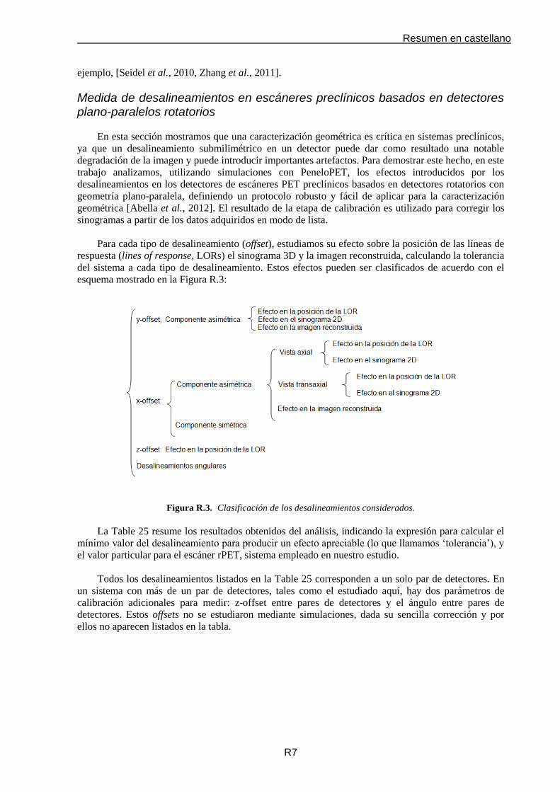
Resumen en castellano
R7
ejemplo, [Seidel et al., 2010, Zhang et al., 2011].
Medida de desalineamientos en escáneres preclínicos basados en detectores plano-paralelos rotatorios
En esta sección mostramos que una caracterización geométrica es crítica en sistemas preclínicos,
ya que un desalineamiento submilimétrico en un detector puede dar como resultado una notable
degradación de la imagen y puede introducir importantes artefactos. Para demostrar este hecho, en este
trabajo analizamos, utilizando simulaciones con PeneloPET, los efectos introducidos por los
desalineamientos en los detectores de escáneres PET preclínicos basados en detectores rotatorios con
geometría plano-paralela, definiendo un protocolo robusto y fácil de aplicar para la caracterización
geométrica [Abella et al., 2012]. El resultado de la etapa de calibración es utilizado para corregir los
sinogramas a partir de los datos adquiridos en modo de lista.
Para cada tipo de desalineamiento (offset), estudiamos su efecto sobre la posición de las líneas de
respuesta (lines of response, LORs) el sinograma 3D y la imagen reconstruida, calculando la tolerancia
del sistema a cada tipo de desalineamiento. Estos efectos pueden ser clasificados de acuerdo con el
esquema mostrado en la Figura R.3:
Figura R.3. Clasificación de los desalineamientos considerados.
La Table 25 resume los resultados obtenidos del análisis, indicando la expresión para calcular el
mínimo valor del desalineamiento para producir un efecto apreciable (lo que llamamos ‘tolerancia’), y
el valor particular para el escáner rPET, sistema empleado en nuestro estudio.
Todos los desalineamientos listados en la Table 25 corresponden a un solo par de detectores. En
un sistema con más de un par de detectores, tales como el estudiado aquí, hay dos parámetros de
calibración adicionales para medir: z-offset entre pares de detectores y el ángulo entre pares de
detectores. Estos offsets no se estudiaron mediante simulaciones, dada su sencilla corrección y por
ellos no aparecen listados en la tabla.

Resumen en castellano
R8
Tabla R.1. Resumen del estudio de los desalineamientos. Para cada tipo de offset la tabla indica la simulación
(tipo de adquisición) empleada para evaluar su efecto en el sinograma y en la imagen, la expresión para
calcular la tolerancia y su valor particular para el escáner rPET. (COR: centro de rotación)
Desalineamiento Adquisición Efecto en el sinograma
Efecto en la imagen Tolerancia
Valor para el escáner rPET
y-offset, afecta al COR (asimétrico)
Fuente puntual no centrada
Gap radial Forma de
media luna Medio pitch 0.8 mm
y-offset, no afecta al COR
(simétrico)
Fuente puntual no centrada
Mayor FWHM en la vista coronal
Pérdida de resolución transaxial
No considerado No considerado
x-offset, afecta al COR (asimétrico)
Fuente puntual en el centro del
FOV
Gap axial, centro de masas
modificado y mayor FWHM en la vista
coronal
Forma de media luna
5.12
1
2 NlRx
7 mm
x-offset, no afecta al COR
(simétrico)
Fuente puntual no centrada
Mayor FWHM en la vista coronal
Pérdida de resolución axial
y transaxial No considerado No considerado
z-offset Cualquier
fuente puntual Mayor FWHM en la
vista sagital Pérdida de
resolución axial Pitch 1.6 mm
‘Tilt’ (eje y) Fuente puntual
no centrada Gap radial
Pérdida de resolución axial )2/(
arctanminl
pitch
14.9º
‘Slant’ (eje z)
Fuente puntual en cualquier
posición conocida
Mayor FWHM en la vista sagital
Forma de media luna )2/(
arctanminl
pitch 14.9º
‘Skew’ Fuente puntual no centrada (x-
y, z)
Gap radial y mayor FWHM en la vista
axial
Pérdida de resolución transaxial y
axial
2/arcsinmin
pitchR
pitch
4.2º
Los resultados de este estudio nos permitieron desarrollar un algoritmo de calibración para
calcular los desalineamientos de los bloques detectores del escáner. Los datos de entrada para el
algoritmo son dos adquisiciones en modo lista de una fuente puntual (en nuestro caso, fuente de 22
Na
de 0.3 mm de diámetro, encapsulada en una caja de epoxi de 1 cm de lado). En la primera adquisición,
la fuente se coloca en el centro del FOV (‘centered acquisition’) y en la segunda la fuente se encuentra
a 11 mm de distancia de ese centro en el plano transaxial (‘non-centered acquisition’). Las
reconstrucciones intermedias se genera por medio de SSRB (span = 1) seguido por una
retroproyección filtrada 2D (2D-FBP) con un filtro rampa. El resultado del algoritmo de calibración es
un fichero que contiene los valores de los desalineamientos. Este fichero es utilizado en
reconstrucciones posteriores para generar un sinograma corregido en el que se traslada la posición de
cada LOR de acuerdo con los desalineamientos estimados. La Figure 58 muestra un diagrama de flujo
del proceso de calibración y la interfaz de la herramienta de calibración al final del proceso.
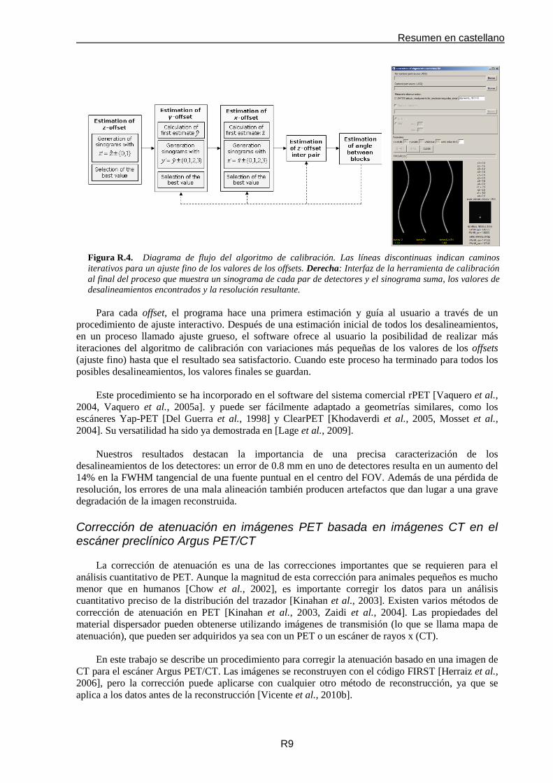
Resumen en castellano
R9
Figura R.4. Diagrama de flujo del algoritmo de calibración. Las líneas discontinuas indican caminos
iterativos para un ajuste fino de los valores de los offsets. Derecha: Interfaz de la herramienta de calibración
al final del proceso que muestra un sinograma de cada par de detectores y el sinograma suma, los valores de
desalineamientos encontrados y la resolución resultante.
Para cada offset, el programa hace una primera estimación y guía al usuario a través de un
procedimiento de ajuste interactivo. Después de una estimación inicial de todos los desalineamientos,
en un proceso llamado ajuste grueso, el software ofrece al usuario la posibilidad de realizar más
iteraciones del algoritmo de calibración con variaciones más pequeñas de los valores de los offsets
(ajuste fino) hasta que el resultado sea satisfactorio. Cuando este proceso ha terminado para todos los
posibles desalineamientos, los valores finales se guardan.
Este procedimiento se ha incorporado en el software del sistema comercial rPET [Vaquero et al.,
2004, Vaquero et al., 2005a]. y puede ser fácilmente adaptado a geometrías similares, como los
escáneres Yap-PET [Del Guerra et al., 1998] y ClearPET [Khodaverdi et al., 2005, Mosset et al.,
2004]. Su versatilidad ha sido ya demostrada en [Lage et al., 2009].
Nuestros resultados destacan la importancia de una precisa caracterización de los
desalineamientos de los detectores: un error de 0.8 mm en uno de detectores resulta en un aumento del
14% en la FWHM tangencial de una fuente puntual en el centro del FOV. Además de una pérdida de
resolución, los errores de una mala alineación también producen artefactos que dan lugar a una grave
degradación de la imagen reconstruida.
Corrección de atenuación en imágenes PET basada en imágenes CT en el escáner preclínico Argus PET/CT
La corrección de atenuación es una de las correcciones importantes que se requieren para el
análisis cuantitativo de PET. Aunque la magnitud de esta corrección para animales pequeños es mucho
menor que en humanos [Chow et al., 2002], es importante corregir los datos para un análisis
cuantitativo preciso de la distribución del trazador [Kinahan et al., 2003]. Existen varios métodos de
corrección de atenuación en PET [Kinahan et al., 2003, Zaidi et al., 2004]. Las propiedades del
material dispersador pueden obtenerse utilizando imágenes de transmisión (lo que se llama mapa de
atenuación), que pueden ser adquiridos ya sea con un PET o un escáner de rayos x (CT).
En este trabajo se describe un procedimiento para corregir la atenuación basado en una imagen de
CT para el escáner Argus PET/CT. Las imágenes se reconstruyen con el código FIRST [Herraiz et al.,
2006], pero la corrección puede aplicarse con cualquier otro método de reconstrucción, ya que se
aplica a los datos antes de la reconstrucción [Vicente et al., 2010b].

Resumen en castellano
R10
La Figura R.5 muestra un diagrama de flujo con las pasos necesarios para corregir la atenuación
en el escáner de Argus usando imágenes CT
Figura R.5. Diagrama de flujo para la corrección de atenuación usando imágenes CT en el escáner
Argus PET/CT
En este trabajo se compara un método de corrección de atenuación simple basado en un cilindro
de agua del tamaño de campo de visión (corrección por defecto incluida en el código FIRST [Herraiz
et al., 2006], algoritmo de reconstrucción empleado para reconstruir las imágenes) con un método más
preciso basado en imágenes CT (el implementado en este trabajo). Del análisis de los resultados
concluimos que la corrección de atenuación basada en imágenes CT no sólo proporciona una mejor
cuantificación, sino que también reduce la 2, lo que significa una mayor coherencia entre la imagen
reconstruida y los datos adquiridos. El procedimiento ha sido incorporado en el software del escáner
comercial Argus PET/CT.
Diseño de prototipos PET preclínicos
Desde el primer escáner PET preclínico [Watanabe et al., 1992], los escáneres PET de pequeños
animales están en continuo desarrollo. Los nuevos sistemas se producen con mayor sensibilidad,
resolución espacial, y capacidad para adquirir tasas de conteo más altas [Wang et al., 2006b, Bao et
al., 2009]. El diseño de un nuevo escáner PET preclínico es un proceso muy complejo que requiere
tomar decisiones sobre un conjunto de aspectos de diferente naturaleza. Las simulaciones Monte Carlo
se han convertido en una herramienta muy valiosa en las primeras etapas del proceso de diseño, lo que
permite realizar estudios exhaustivos, teniendo en cuenta todos los componentes que forman el escáner
[Heinrichs et al., 2003].
Además de la simulación de los datos, es necesario desarrollar métodos de reconstrucción
necesarios para procesar correctamente estos datos con el fin de obtener parámetros importantes del
rendimiento del sistema, tales como la resolución espacial, y para evaluar la calidad de las imágenes
finales. Para ello, los métodos de reconstrucción existentes tienen que ser modificados y ampliados
para poder adaptarse a la geometría no convencional de algunos diseños.
Ejemplos de estas modificaciones en la simulación y en la reconstrucción se presentan en este
capítulo. El propósito de este capítulo es el estudio, por medio de simulaciones Monte Carlo, de las
principales características y las posibles modificaciones de dos nuevos prototipos preclínicos en fase
de desarrollo en dos centros diferentes, donde el autor de esta tesis estuvo trabajando como parte del
programa de estancias breves de la beca JAEPredoctoral (2008).
Datos PET
Datos CT Imagen CT (unidades
Hounsfield) (resolución CT)
Mapa de atenuación para rayos gamma de 511 keV
(resolución PET)
Reconstrucción de la imagen
Transformación (CT) (PET) usando aproximación bilineal
ACFs
Datos PET corregidos por
atenuación
Aplicación de la corrección
(LOR a LOR)
Proyección del mapa de atenuación y cálculo de los
ACFs
Imagen PET corregida
por atenuación
Reconstrucción de la imagen
Argus PET/CT

Resumen en castellano
R11
Escáner Zoom-in PET
En esta sección estudiamos el potencial de un nuevo prototipo, el ‘Zoom-in PET’ (o ZiPET),
propuesto y diseñado por el Department of Biomedical Engineering, University of California, (Davis,
CA) [Zhou and Qi, 2009, 2010, 2011, Qi et al., 2011]. El sistema integra un detector de alta resolución
en un escáner de microPET existente que actúa de forma análoga a una lupa para obtener datos de alta
resolución de una pequeña parte del campo de visión definidos por una región de interés alrededor de
la cara frontal del inserto (ver Figure 70). El diseño propuesto puede ofrecer una solución costo-
efectiva para obtener imágenes de alta resolución para una región específica, sin la construcción de un
sistema de anillo completo. Tal sistema puede ser útil para el estudio del cáncer usando modelos
animales donde los tumores son a menudo cultivados cerca de la superficie de la piel y por lo tanto,
permitir un cercano contacto con el detector de alta resolución. La Figure 70 muestra un esquema del
prototipo simulado en este trabajo con el inserto de alta resolución situado en el centro de la dirección
axial del escáner microPET II [Tai et al., 2003].
Figura R.6. Vistas 2D (plano transaxial) [izquierda] y 3D [derecha] del escánere Zoom-in PET
simulado en este trabajo.
El escáner comercial microPET II (PET en lo que sigue) consta de tres anillos axiales de
detectores con un diámetro de 160 mm, cada uno formado por 30 módulos de detectores. Sin embargo,
en este trabajo sólo se consideró uno de los tres anillos axiales para las simulaciones. Cada módulo
detector de PET consiste en una matriz de 14×14 de 1.0×1.0×12.5 mm3 de cristales de LSO. La
caracterización del escáner microPET II se ha publicado en [Tai et al., 2003] y [Yang et al., 2004].
El detector de alta resolución (inserto en lo que sigue) está compuesto por una matriz de 64×64 de
dimensiones 0.3×0.3×20 mm3 de cristales de LSO y puede proporcionar profundidad de interacción
(DOI) para reducir los errores de paralaje. El DOI se obtiene utilizando una doble lectura, en las que
los fotones ópticos generados por la matriz de cristales de centelleo son leídos por dos fotodiodos de
avalancha sensibles a la posición (PSAPDs) uno en la parte delantera y la otra en el extremo posterior
del detector [Yang et al., 2006]. El valor del DOI se calcula tomando la relación de las señales de los
dos PSAPDs proporcionar una medida continua de DOI para cada evento registrado.
En este trabajo utilizamos simulaciones Monte Carlo con el paquete de simulación PeneloPET
[España et al., 2009] para caracterizar el impacto de la introducción del detector de alta resolución
(inserto) en el rendimiento del sistema, a excepción del aumento de la resolución espacial, que ya fue
estudiado en trabajos anteriores con un análisis teórico y simulaciones básicas [Zhou and Qi, 2009], y
mediciones experimentales [Qi et al., 2011]. Para este fin, fue necesario introducir varias
modificaciones en el código PeneloPET debido a la geometría no estándar del sistema con dos
conjuntos diferentes de bloques detectores en diferentes posiciones radiales. En concreto las
modificaciones incorporadas fueron:

Resumen en castellano
R12
1. En la definición de la geometría del escáner. Es necesario definir dos tipos de detectores:
el anillo de detectores del escáner MicroPET II y el inserto de alta resolución.
2. Incluir la definición explícita de la matriz de coincidencias, que indica los bloques que se
encuentran en coincidencia durante la adquisición, permitiendo coincidencias entre
bloques del anillo de MicroPET II y entre el inserto y los detectores del anillo.
3. Acceso dinámico a la información de los parámetros de cada tipo de detector para cargar
las propiedades adecuadas en cada interacción de un fotón en un bloque detector.
4. Modelado especial de la profundidad de interacción (DOI) para simular más precisamente
el sistema de doble lectura del sistema real mediante PSAPDs.
5. Nuevos formatos para los archivos de salida para poder separar los datos de alta
resolución (coincidencias entre el inserto y los detectores del anillo de MicroPET II) y los
datos de baja resolución (coincidencias entre bloques del anillo)
La evaluación del rendimiento del sistema se centra en la sensibilidad, la capacidad de
profundidad de interacción (DOI) del inserto y la curva NEC, ya que la resolución espacial se midió en
trabajos anteriores [Zhou and Qi, 2009 2011] demostrando su mejora. De los resultados se puede
afirmar que existe una evidente mejora en la sensibilidad cuando el inserto está incluido en el sistema.
A pesar de esto, el diseño del sistema puede ser mejorado, dado que se ha demostrado, del análisis de
las curvas NEC y de la sensibilidad, que el diseño actual con sólo un anillo axial en el sistema PET y
el tamaño propuesto para el inserto no proporcionan un rendimiento óptimo, ya que el número de
coincidencias no deseadas como pile-up, randoms, auto-coincidencias y de scatter, aumenta
drásticamente con la presencia del inserto. El análisis de la profundidad de interacción del inserto
también sugiere la utilización de cristales más cortos, por ejemplo reduciendo su longitud 5 mm, lo
que supone una menor degradación de la resolución a expensas de una pérdida pequeña de
sensibilidad.
Estos resultados muestran un ejemplo de cómo los datos simulados pueden ayudar a guiar el
diseño de nuevos prototipos, analizando todas las ventajas y desventajas antes de tomar una decisión
final. En nuestro estudio, los resultados sugieren modificar la geometría del sistema incluyendo, por
ejemplo, más anillos axiales en microPET II y tratar de blindar de alguna manera el inserto para evitar
la detección de singles desde fuera del campo de visión axial.
Escáner NIH PPI
El escáner NIH PPI (‘positron projection imager’) fue diseñado como una opción de bajo coste
para estudios con ratones [Seidel et al., 2010]. El prototipo consta de dos detectores opuestos en
coincidencia temporal compuestos de cristales pixelados de LYSO, montados en un dispositivo que
permite tres separaciones entre los módulos: 39, 29 y 19 mm. El objeto/animal en estudio se coloca
sobre una placa de plástico situado entre los detectores, los cuales se mantienen inmóviles durante la
adquisición, haciendo al escáner PPI un sistema tomográfico de ángulo limitado. El campo de visión
abarcado por los detectores es suficientemente grande para poder adquirir la imagen de todo el cuerpo
de un ratón en una sola proyección.
Cada bloque detector está compuesto por una matriz de 2659 cristales, cada uno con un tamaño
de 1.51.512 mm3 y un pitch de 1.6 mm. La matriz de cristales está ópticamente acoplada (mediante
una grasa óptica) a un fotomultiplicador sensible a posición (modelo H8500C de Hamamatsu Corp.,
Bridgewater, NJ).
En este trabajo, se realiza un análisis cuantitativo del rendimiento del sistema en términos de
sensibilidad, resolución y calidad de imagen mediante simulaciones Monte Carlo (utilizando
PeneloPET). A pesar de que el escáner fue diseñado inicialmente para obtener imágenes en proyección

Resumen en castellano
R13
(2D), también exploramos la posibilidad de imágenes en 3D del sistema, evaluando la resolución
espacial en diferentes posiciones del FOV y la calidad de las imágenes con adquisiciones reales. Con
este fin, se implementaron distintas aproximaciones desarrollando diferentes métodos de
reconstrucción, desde métodos que proporcionan imágenes planares, sin información en la dirección Z,
hasta métodos más precisos en modo 3D basados en el código GFIRST [Herraiz et al., 2011] con tres
aproximaciones diferentes:
En la primera, se utilizó una versión simplificada de la matriz de probabilidad, despreciando
los efectos de resolución. Este método se empleó para medir la resolución espacial del sistema
ya que la calidad de las imágenes resultantes es comparable, en términos de resolución
espacial, a una reconstrucción FBP, el método de reconstrucción estándar para medir la
resolución espacial en los escáneres PET.
En el segundo método 3D, se incluyeron los efectos de resolución utilizando un kernel
invariante de emborronamiento usando la PSF medida en fuentes puntuales reconstruidas con
el método sin recuperación de resolución. Este kernel se usa con distinto ancho en la
proyección y retroproyección para aumentar la velocidad de convergencia del algoritmo.
Finalmente, se desarrolló un nuevo método 3D, mejorando el último método descrito con un
componente de emborronado adicional para regularizar la convergencia en direcciones X e Y
[Vicente et al., 2012b].
Figura R.7. Izquierda: Esquema simplificado de la geometría del escáner NIH PPI. Derecha: Fotografía
del prototipo.
La caracterización realizada en este trabajo ha demostrado que el sistema PPI tiene valores de
sensibilidades muy competitivos, siendo algunos valores experimentales de la sensibilidad en el centro
del FOV por ejemplo: 10% a 100-650 keV, 7% a 250-650 keV y 5% a 400-650 keV. Estos resultados
mejoran la sensibilidad del sistema PETbox [Zhang et al., 2010, Zhang et al., 2011], obteniendo un
valor de sensibilidad para el PPI en 400-650 keV similar a la del PETbox en 100-650 keV. El sistema
PPI también mejora la mayoría de los valores de sensibilidad de los escáneres de anillo completo. Con
respecto a las medidas de resolución, el sistema tiene alta resolución en el plano XY con valores
inferiores a 1.8 mm y prácticamente uniforme en todo el FOV. Sin embargo, la falta de datos en la
dirección Z da como resultado una degradación de la resolución del sistema en dicha dirección, con
valores en su mayoría por encima de 6 mm cuando no aplicamos recuperación de resolución en la
reconstrucción. Estas diferencias se reducen utilizando la información de la PSF en la reconstrucción,
obteniendo una resolución en Z todavía peor que en las otras direcciones, pero con valores menores de
1.8 mm en la dirección Z y por debajo de 1.4 mm en las otras dos direcciones.
Por último, las imágenes iniciales obtenidas, utilizando los métodos de reconstrucción antes
mencionados, demuestran las capacidades de imagen del sistema PPI y el potencial del nuevo método

Resumen en castellano
R14
de reconstrucción con regularización, empleado para converger a imágenes con las propiedades
deseadas.
Conclusiones
La investigación preclínica PET es una técnica compleja que ha ganado un creciente impacto en
los últimos años, especialmente debido al desarrollo de sistemas PET específicos para pequeños
animales. Quedan, sin embargo, retos importantes con respecto a la instrumentación, evaluación de
datos y experimentación, que son necesarios superar con el fin de alcanzar datos preclínicos
cuantitativos y fiables.
En esta tesis se han presentado aportaciones originales al estudio de las fuentes de error que
limitan la calidad de las imágenes PET aportando nuevos métodos y algoritmos para compensar sus
efectos y mejoras en las simulaciones Monte Carlo y en los métodos de reconstrucción para adaptar
los códigos existentes a las geometrías no-convencionales de algunos diseños.
Las principales contribuciones de esta tesis son:
1. Una evaluación detallada del rendimiento de dos escáneres PET preclínicos con geometrías y
características muy diferentes, el escáner SEDECAL rPET y el SEDECAL Argus,
argumentando la importancia de tener protocolos estandarizados para garantizar una
caracterización precisa. Se ha mostrado una comparación crítica de las características de los
escáneres, comparándolas a su vez con otros escáneres PET preclínicos disponibles en el
mercado, mostrando que ambos escáneres tienen prestaciones muy competitivas que mejoran
en algunos parámetros las de otros sistemas comerciales.
2. Se ha demostrado que estos protocolos de caracterización no son perfectos, analizando en
detalle algunos ejemplos y, con la ayuda de simulaciones muy detalladas y realistas, se han
propuesto mejoras en los procedimientos. Un ejemplo es la propuesta de mejora del estándar
NEMA para medir la fracción de dispersión, de manera que sea independiente del isótopo
empleado en términos de rango de positrón. Esta extensión del protocolo NEMA incluye una
desconvolución de los perfiles empleados en el método con una distribución unidimensional
del rango del positrón con el fin de eliminar los efectos del rango. Este nuevo protocolo ha sido
probado usando 68
Ga, un radionúclido con rango de positrón grande, obteniendo los mismos
resultados que con 18
F, el isótopo propuesto por NEMA.
3. De las limitaciones observadas en los escáneres evaluados, se han desarrollado nuevos
métodos y algoritmos relevantes no sólo para estos escáneres particulares, sino fácilmente
adaptables a diferentes arquitecturas. En concreto:
3.1. Un método para linealizar las tasas de coincidencias totales eliminando efectos no lineales
debidos a las pérdidas por tiempo muerto y pile-up y a las ganancias debidas al pile-up
dentro de la ventana de energía seleccionada. El método está basado en la relación lineal
entre el tiempo muerto efectivo (que tiene en cuenta los efectos de tiempo muerto y pile-
up), y la relación de singles con respecto a las coincidencias (Singles-to-Coincidences ratio
SCR). Los resultados muestran que usando dicho método, la precisión en las tasas
corregidas es inferior al 7%, incluso para actividades altas, evitando el sesgo introducido
cuando se emplea un procedimiento uniparametral. El método ha sido validado usando
datos reales y simulados de los escáneres rPET y Argus.
3.2. Un protocolo de calibración, desarrollado e implementado en una herramienta de software,
para compensar el efecto de los pequeños desalineamientos mecánicos en los sistemas PET
preclínicos con detectores plano-paralelos rotatorios. Esta herramienta de calibración
determina los desalineamientos dentro de una tolerancia aceptable en cada parámetro
Resumen en castellano
R15
geométrico. Los resultados han destacado la importancia de una precisa caracterización
geométrica mostrando la aparición de artefactos y una importante pérdida de resolución en
la imagen final si los desalineamientos en los detectores no son apropiadamente corregidos.
3.3. Una corrección de atenuación basada en imágenes de tomografía computarizada (CT). Los
resultados han mostrando una mejora en las imágenes corregidas en términos de
cuantificación y mayor consistencia entre los datos adquiridos y los estimados en la
reconstrucción que cuando se emplean métodos más sencillos, como por ejemplo la
corrección basada en un cilindro de agua del tamaño del campo de visión del escáner.
4. Haciendo uso de toda la experiencia adquirida en la caracterización de los escáneres y el estudio
de las fuentes de error que limitan la calidad de las imágenes, se han utilizado simulaciones
Monte Carlo para guiar el diseño de nuevos prototipos, realizando las modificaciones necesarias
en los códigos Monte Carlo y en los métodos de reconstrucción empleados para adaptar los
códigos existentes a la geometría no convencional de los nuevos diseños. En concreto, los
escáneres estudiados son:
4.1. Zoom-in PET: un detector de alta resolución introducido en el FOV del escáner microPET
II (con sólo un anillo de detectores). Las simulaciones empleadas en este estudio se han
realizado en una versión modificada de PeneloPET, que fue desarrollada para permitir la
simulación de la geometría particular de este prototipo. Este estudio es un ejemplo de cómo
las simulaciones Monte Carlo pueden ayudar al diseño de nuevos prototipos, analizando las
ventajas y desventajas del sistema antes de tomar la decisión final. En concreto, los
resultados de la caracterización de este prototipo sugieren una modificación de la geometría
añadiendo, por ejemplo, más anillos de detectores al escáner MicroPET II y tratando de
blindar el inserto para evitar la detección de singles provenientes de fuera del FOV.
4.2. NIH PPI: escáner de bajo coste y alta sensibilidad consistente en dos detectores no
rotatorios. Esta geometría hace que el prototipo tenga un muestreo pobre en la dirección de
separación de los detectores, por lo que es necesario desarrollar nuevas aproximaciones y
métodos de reconstrucción, como el presentado en esta tesis, que emplea una convolución
regularizada para hacer la convergencia más isotrópica. La caracterización del prototipo ha
demostrado que el sistema cumple con las especificaciones deseadas y las imágenes
iniciales obtenidas, su capacidad de imagen 3D y el potencial del nuevo método de
regularización desarrollado.
En resumen, esta tesis muestra la importancia de simulaciones Monte Carlo detalladas en la
mejora del rendimiento de los escáneres existentes y de los protocolos de caracterización de los
mismos, así como en el diseño de nuevos prototipos.
Los resultados descritos en las conclusiones 3.2 y 3.3 han sido transferidos a la industria y han
sido integrados en los escáneres preclínicos de alta resolución fabricados por SEDECAL (Madrid,
España) y distribuidos mundialmente.

Resumen en castellano
R16
Referencias Abella, M., Vicente, E., Rodríguez-Ruano, A., España, S., Lage, E., Desco, M., Udias, J. M. & Vaquero, J. J. 2012.
Misalignments calibration in small-animal PET scanners based on rotating planar detectors and parallel-beam
geometry. Phys Med Biol (Submitted).
Bao, Q., Newport, D., Chen, M., Stout, D. B. & Chatziioannou, A. F. 2009. Performance evaluation of the inveon dedicated
PET preclinical tomograph based on the NEMA NU-4 standards. J Nucl Med, 50, 401-8.
Blanco, A. 2006. Positron Range Effects on the Spatial Resolution of RPC-PET. In: Nuclear Science Symposium
Conference Record, 2006. IEEE, Oct. 29 2006-Nov. 1 2006 2006. 2570-2573.
Bloomfield, P. M., Rajeswaran, S., Spinks, T. J., Hume, S. P., Myers, R., Ashworth, S., Clifford, K. M., Jones, W. F., Byars,
L. G., Young, J. & et al. 1995. The design and physical characteristics of a small animal positron emission
tomograph. Phys Med Biol, 40, 1105-26.
Brownell, G. L., Burnham, C. A., Wilensky, S., Aronow, S., Kazemi, H. & Streider , D. 1969. New developments in positron
scintigraphy and the application of cyclotron produced positron emitters. In: Medical Radioisotope Scintigraphy,
1969 Vienna, Austria. International Atomic Energy Agency, 163–176.
Burnham, C. A. & Brownell, G. L. 1972. A Multi-Crystal Positron Camera. Nuclear Science, IEEE Transactions on, 19, 201-
205.
Cal-Gonzalez, J., Herraiz, J. L., Espana, S., Desco, M., Vaquero, J. J. & Udias, J. M. 2010. Validation of PeneloPET positron
range estimations. In: Nuclear Science Symposium Conference Record (NSS/MIC), 2010 IEEE, Oct. 30 2010-
Nov. 6 2010 2010. 2396-2399.
Chow, P. L., Rannou, R. & Chatziioannou, A. 2002. Attenuation correction for a 3D small animal PET tomograph, using x-
ray microCT. Mol. Imag. Biol., 4, S17–S18.
Del Guerra, A., Bartoli, A., Belcari, N., Herbert, D., Motta, A., Vaiano, A., Di Domenico, G., Sabba, N., Moretti, E.,
Zavattini, G., Lazzarotti, M., Sensi, L., Larobina, M. & Uccelli, L. 2006. Performance evaluation of the fully
engineered YAP-(S)PET scanner for small animal imaging. Nuclear Science, IEEE Transactions on, 53, 1078-
1083.
Del Guerra, A., Di Domenico, G., Scandola, M. & Zavattini, G. 1998. YAP-PET: first results of a small animal positron
emission tomograph based on YAP:Ce finger crystals. Nuclear Science, IEEE Transactions on, 45, 3105-3108.
España, S., Herraiz, J. L., Vicente, E., Herranz, E., Vaquero, J. J., Desco, M. & Udias, J. M. 2007. Improved image
reconstruction in small animal PET using a priori estimates of single-pixel events. In: Nuclear Science Symposium
Conference Record, 2007. NSS '07. IEEE, Oct. 26 2007-Nov. 3 2007 2007. 3876-3880.
España, S., Herraiz, J. L., Vicente, E., Vaquero, J. J., Desco, M. & Udias, J. M. 2009. PeneloPET, a Monte Carlo PET
simulation tool based on PENELOPE: features and validation. Phys Med Biol, 54, 1723-42.
Goertzen, A. L., Bao, Q., Bergeron, M., Blankemeyer, E., Blinder, S., Cañadas, M., Chatziioannou, A. F., Dinelle, K.,
Elhami, E., Jans, H.-S., Lage, E., Lecomte, R., Sossi, V., Surti, S., Tai, Y.-C., Vaquero, J. J., Vicente, E., Williams,
D. A. & Laforest, R. 2012. NEMA NU 4-2008 Comparison of Preclinical PET Imaging Systems. The Journal of
Nuclear Medicine (Accepted).
Heinrichs, U., Pietrzyk, U. & Ziemons, K. 2003. Design optimization of the PMT-ClearPET prototypes based on simulation
studies with GEANT3. Nuclear Science, IEEE Transactions on, 50, 1428-1432.
Herraiz, J. L., Espana, S., Vaquero, J. J., Desco, M. & Udias, J. M. 2006. FIRST: Fast Iterative Reconstruction Software for
(PET) tomography. Phys Med Biol, 51, 4547-65.
Herraiz, J. L., España, S., Cabido, R., Montemayor, A. S., Desco, M., Vaquero, J. J. & Udias, J. M. 2011. GPU-Based Fast
Iterative Reconstruction of Fully 3-D PET Sinograms. Nuclear Science, IEEE Transactions on, 58, 2257-2263.
Khodaverdi, M., Weber, S., Streun, M., Parl, C., Larue, H., Brandenburg, G., Bauer, A., Dehnhardt, M., Auffray, E.,
Boutemeur, M., Bruyndonckx, P., Choi, Y., D'Asseler, Y., Devroede, O., Dujardin, C., Fedorov, A., Heinrichs, U.,
Janier, M., Jung, J. H., Korjik, M., Krieguer, M., Largeron, G., Lartizien, C., Lecoq, P., Lemaitre, C., Leonard, S.,
Loude, J. F., Morel, C., Mosset, J. B., Pedrini, C., Petrosyan, A. G., Rey, M., Sappey-Marinier, D., Roldan, P. S.,
Simon, L., Song, T. Y., Staelens, S., Tavernier, S., Trummer, J., Van Holen, R., Vieira, J. M., Wieers, E.,
Wisniewska, M., Wisniewski, D., Wu, Y., Pietrzyk, U. & Ziemons, K. 2005. High resolution imaging with
ClearPET™ Neuro - first animal images. In: Nuclear Science Symposium Conference Record, 2005 IEEE,
23-29 Oct. 2005 2005. 4 pp.
Kinahan, P. E., Hasegawa, B. H. & Beyer, T. 2003. X-ray-based attenuation correction for positron emission
tomography/computed tomography scanners. Semin Nucl Med, 33, 166-79.
Knoll, G. F. 2000. Radiation detection and measurement / Glenn F. Knoll, New York :, Wiley.
Lage, E., Vaquero, J. J., Sisniega, A., Espana, S., Tapias, G., Abella, M., Rodriguez-Ruano, A., Ortuno, J. E., Udias, A. &
Desco, M. 2009. Design and performance evaluation of a coplanar multimodality scanner for rodent imaging. Phys
Med Biol, 54, 5427-41.
Mosset, J. B., Devroede, O., Krieguer, M., Rey, M., Vieira, J. M., Jung, J. H., Kuntner, C., Streun, M., Ziemons, K., Auffray,
E., Sempere-Roldan, P., Lecoq, P., Bruyndonckx, P., Loude, J. F., Tavernier, S. & Morel, C. 2004. Development of
an optimised LSO/LuYAP phoswich detector head for the ClearPET camera. In: Nuclear Science Symposium
Conference Record, 2004 IEEE, 16-22 Oct. 2004 2004. 2439-2443 Vol. 4.
National Electrical Manufacturers Association (NEMA). 1994. Performance Measurements of Positron Emission
Tomographs. NEMA Standards Publication NU2-1994. Rosslyn, VA. National Electrical Manufacturers
Association
National Electrical Manufacturers Association (NEMA). 2001. Performance Measurements of Positron Emission
Tomographs. NEMA Standards Publication NU2-2001. Rosslyn, VA. National Electrical Manufacturers

Resumen en castellano
R17
Association
National Electrical Manufacturers Association (NEMA). 2008. Performance Measurements of Small Animal Positron
Emission Tomographs. NEMA Standards Publication NU4-2008. Rosslyn, VA. National Electrical Manufacturers
Association
Pavlopoulos, S. & Tzanakos, G. 1993. Design and performance evaluation of a high resolution small animal positron
tomograph. In: Nuclear Science Symposium and Medical Imaging Conference, 1993., 1993 IEEE Conference
Record., 31 Oct-6 Nov 1993 1993. 1697-1701 vol.3.
Pavlopoulos, S. & Tzanakos, G. 1996. Design and performance evaluation of a high-resolution small animal positron
tomograph. Nuclear Science, IEEE Transactions on, 43, 3249-3255.
Phelps, M. E., Hoffman, E. J., Mullani, N. A. & Ter-Pogossian, M. M. 1975. Application of annihilation coincidence
detection to transaxial reconstruction tomography. J Nucl Med, 16, 210-24.
Qi, J., Yang, Y., Zhou, J., Wu, Y. & Cherry, S., R. 2011. Experimental assessment of resolution improvement of a zoom-in
PET. Physics in Medicine and Biology, 56, N165.
Rogers, D. W. 2006. Fifty years of Monte Carlo simulations for medical physics. Phys Med Biol, 51, R287-301.
Seidel, J., Wenze, X., Kakareka, J. W., Pohida, T. J., Green, M. V. & Choyke, P. L. 2010. A positron projection imager for
whole-body mouse imaging. In: Nuclear Science Symposium Conference Record (NSS/MIC), 2010 IEEE, Oct. 30
2010-Nov. 6 2010 2010. 2206-2209.
Sweet, W. H. 1951. The uses of nuclear disintegration in the diagnosis and treatment of brain tumor. N Engl J Med, 245, 875-
8.
Tai, Y. C., Chatziioannou, A. F., Yang, Y., Silverman, R. W., Meadors, K., Siegel, S., Newport, D. F., Stickel, J. R. &
Cherry, S. R. 2003. MicroPET II: design, development and initial performance of an improved microPET scanner
for small-animal imaging. Phys Med Biol, 48, 1519-37.
Ter-Pogossian, M. M., Phelps, M. E., Hoffman, E. J. & Mullani, N. A. 1975. A positron-emission transaxial tomograph for
nuclear imaging (PETT). Radiology, 114, 89-98.
Tzanakos, G. & Pavlopoulos, S. 1993. Design and performance evaluation of a new high resolution detector array module for
PET. In: Nuclear Science Symposium and Medical Imaging Conference, 1993., 1993 IEEE Conference Record.,
31 Oct-6 Nov 1993 1993. 1842-1846 vol.3.
Vaquero, J. J., Lage, E., Ricon, L., Abella, M., Vicente, E. & Desco, M. 2005a. rPET detectors design and data processing.
In: Nuclear Science Symposium Conference Record, 2005 IEEE, 23-29 Oct. 2005 2005a. 2885-2889.
Vaquero, J. J., Lage, E., Ricón, L., Abella, M., Vicente, E. & Desco, M. 2005b. rPET Detectors Design and Data Processing.
IEEE Nuclear Science Symposium Conference Record.
Vaquero, J. J., Molins, A., Ortuño, J., Pascau, J. & Desco, M. 2004. Preliminary results of the small animal rotational
positron emission tomography scanner. In: Mol. Imag. Biol., 2004. 102.
Vicente, E., Herraiz, J. L., Canadas, M., Cal-Gonzalez, J., Espana, S., Desco, M., Vaquero, J. J. & Udias, J. M. 2010a.
Validation of NEMA NU4-2008 Scatter Fraction estimation with 18F and 68Ga for the ARGUS small-animal PET
scanner. In: Nuclear Science Symposium Conference Record (NSS/MIC), 2010 IEEE, Oct. 30 2010-Nov. 6 2010
2010a. 3553-3557.
Vicente, E., Herraiz, J. L., España, S., Herranz, E., Desco, M., Vaquero, J. J. & Udías, J. M. 2012a. Improved effective dead-
time correction for PET scanners: Application to small-animal PET. Phys Med Biol (Submitted).
Vicente, E., Herraiz, J. L., Seidel, J., Green, M. V., Desco, M., Vaquero, J. J. & Udias, J. M. 2012b. Regularization of 3D
Iterative Reconstruction for a Limited-Angle PET Tomograph. In: Nuclear Science Symposium Conference
Record (NSS/MIC), 2012 IEEE (Accepted), 2012b.
Vicente, E., Udías, A. L., Herraiz, J. L., Desco, M., Vaquero, J. J. & Udías, J. M. 2010b. Corrección de atenuación de
imágenes PET usando datos de TAC en el escáner para animales pequeños Argus PET/CT. Libro de Actas,
CASEIB 2010.
Vicente, E., Vaquero, J. J., Lage, E., Tapias, G., Abella, M., Herraiz, J. L., España, S., Udías, J. M. & Desco, M. 2006
Caracterización del Tomógrafo de Animales rPET. Libro de Actas, CASEIB 2006.
Wang, G. C., Huber, J. S., Moses, W. W., Qi, J. & Choong, W. S. 2006a. Characterization of the LBNL PEM camera.
Nuclear Science, IEEE Transactions on, 53, 1129-1135.
Wang, Y., Seidel, J., Tsui, B. M., Vaquero, J. J. & Pomper, M. G. 2006b. Performance evaluation of the GE healthcare
eXplore VISTA dual-ring small-animal PET scanner. J Nucl Med, 47, 1891-900.
Watanabe, M., Uchida, H., Okada, H., Shimizu, K., Satoh, N., Yoshikawa, E., Ohmura, T., Yamashita, T. & Tanaka, E. 1992.
A high resolution PET for animal studies. Medical Imaging, IEEE Transactions on, 11, 577-580.
Wu, Y., Bowen, S. L., Yang, K., Packard, N., Fu, L., Burkett, G., Qi, J., Boone, J. M., Cherry, S. R. & Badawi, R. D. 2009.
PET characteristics of a dedicated breast PET/CT scanner prototype. Phys Med Biol, 54, 4273-87.
Yamamoto, S., Amano, M., Miura, S., Iida, H. & Kanno, I. 1986. Deadtime correction method using random coincidence for
PET. J Nucl Med, 27, 1925-8.
Yang, Y. & Cherry, S. R. 2006. Observations regarding scatter fraction and NEC measurements for small animal PET.
Nuclear Science, IEEE Transactions on, 53, 127-132.
Yang, Y., Dokhale, P. A., Silverman, R. W., Shah, K. S., McClish, M. A., Farrell, R., Entine, G. & Cherry, S. R. 2006. Depth
of interaction resolution measurements for a high resolution PET detector using position sensitive avalanche
photodiodes. Phys Med Biol, 51, 2131-42.
Yang, Y., Tai, Y. C., Siegel, S., Newport, D. F., Bai, B., Li, Q., Leahy, R. M. & Cherry, S. R. 2004. Optimization and
performance evaluation of the microPET II scanner for in vivo small-animal imaging. Phys Med Biol, 49, 2527-45.
Zaidi, H., Montandon, M. L. & Slosman, D. O. 2004. Attenuation compensation in cerebral 3D PET: effect of the attenuation
map on absolute and relative quantitation. Eur J Nucl Med Mol Imaging, 31, 52-63.
Zhang, H., Bao, Q., Vu, N. T., Silverman, R. W., Taschereau, R., Berry-Pusey, B. N., Douraghy, A., Rannou, F. R., Stout, D.

Resumen en castellano
R18
B. & Chatziioannou, A. F. 2011. Performance evaluation of PETbox: a low cost bench top preclinical PET scanner.
Mol Imaging Biol, 13, 949-61.
Zhang, H., Vu, N. T., Bao, Q., Silverman, R. W., Berry-Pusey, B. N., Douraghy, A., Williams, D. A., Rannou, F. R., Stout,
D. B. & Chatziioannou, A. F. 2010. Performance Characteristics of BGO Detectors for a Low Cost Preclinical PET
Scanner. Nuclear Science, IEEE Transactions on, 57, 1038-1044.
Zhou, J. & Qi, J. 2009. Theoretical analysis and simulation study of a high-resolution zoom-in PET system. Physics in
Medicine and Biology, 54, 5193.
Zhou, J. & Qi, J. 2010. Efficient system modeling of a high-resolution zoom-in PET scanner. In: Nuclear Science
Symposium Conference Record (NSS/MIC), 2010 IEEE, Oct. 30 2010-Nov. 6 2010 2010. 3501-3505.
Zhou, J. & Qi, J. 2011. Adaptive Imaging for Lesion Detection Using a Zoom-in PET System. Medical Imaging, IEEE
Transactions on, 30, 119-130.