UnitII Canonical and grand canonical ensembles

8/7/2019 UnitII Canonical and grand canonical ensembles

http://slidepdf.com/reader/full/unitii-canonical-and-grand-canonical-ensembles 1/22

UNIT - 2

Canonical ensemble & Grand-Canonical Ensemble

Microcanonical ensemble deals with the simplest system ie, isolated system and worked on

the hypothesis of equal – a - priori probability. But in actual practice, an isolated system does not occur

in laboratory and hence is of little practical interest except that other ensembles can be constructed

with microcanonical ensemble.

If we replace the constant energy constraint of microcanonical ensemble with constant

temperature constraint, we would have a system defined by parameters (N,V,T). This constant

temperature constraint will work only if the system is in thermal contact with a large heat reservoir.

Thus thermal energy flows between the system and the reservoir and hence the energy of the system

does not remain a constant. The reservoir is considered to be very large and so the energy transferbetween it and the system does not change its energy noticeably. The ensemble of such a system which

exchanges energy with a reservoir is called canonical ensemble. But the system does not share particles

with the reservoir. Thus the total number of particles and volume remains the same for the system as

well as the reservoir.

Let the reservoir at temperature T has energy Er and the system under observation be in the ith

energy level Ei. The system under observation along with the reservoir form a composite system with

constant energy Ee = Er + Ei. This composite system can be treated as a single isolated system, to which

the method of microcanonical ensemble can be applied. If c is the probability that the composite

system is in the region of t-space between ergodic surfaces Ec and Ec + D. let this volume be Dtc. Then

c (Ec) µ Dtc (Ec, Ei) = Dts (Ei) Dtr (Er)

= 0, otherwise (if Ec < E < Ec + D

where Ei is the unperturbed energy of the ith

quantum level of the system. The number of states

accessible to the composite system will be equal to the number of states accessible to the reservoir ‘r’,

since Ei << Er

ie, µ Dtr (Ec - Ei) ---- (2) (when Dtr is large , Dts will also be large, since both the systems

together will be in equilibrium.

Here i is the probability that the system is in the ith

quantum state. Since Ei <<Ec we can expand

Generated by Foxit PDF Creator © Foxit Softwarehttp://www.foxitsoftware.com For evaluation only.



lnDt (Ec- Ei) about Ec = Er into a Taylor series.

Thus lnDt (Ec - Ei) = ln Dtr(Ec) - ln ∆()

Terms with higher powers of Ei can be neglected and thus the above equation would become

ln Dtc (Ec-Ei) = ln Dtr (Ec)-ln Dtr (Er) = ln Dtr (Ec) - bEi --- (3)

Where b= ln∆()| = ----- (4)

where T is the temperature of the reservoir.

Taking exponential of equation (3), we get

Dtr (Ec - Ei) = Dtr (Ec) ----- (5)

Or Pi = C ----- (6)

where C = Dtr (Ec) x some constant a constant. This constant is independent of Ei and is determined

from the normalization condition

=

= 1

∴ = -------- (7)

Thus the probability distribution is given by

Pi (N,V,T) =(,) (,,) ------- (8)

Where = ∑ (,) is called the partition function of the system




The canonical distribution is shown in figure above. It can be seen that higher the energy value,

the less likely the system to be in that state. But all the n-particle quantum states with same energy have

the same probability.

So, we can say that a canonical ensemble is constructed out of many microcanonical ensembles,

one representing each energy level and weighed according to equation (6). The probability of finding the

system in a given energy level Ei is the sum of the probabilities of all states having this energy. The

number of such states is the degeneracy of the level given by Ω(Ei). Thus the probability that the system

is in the ith

state is

= Ω () = Ω () -

As is the product of an exponentially decreasing curve and a rapidly increasing curve, there is a sharp

peak over a narrow range of energy as shown in figure below.




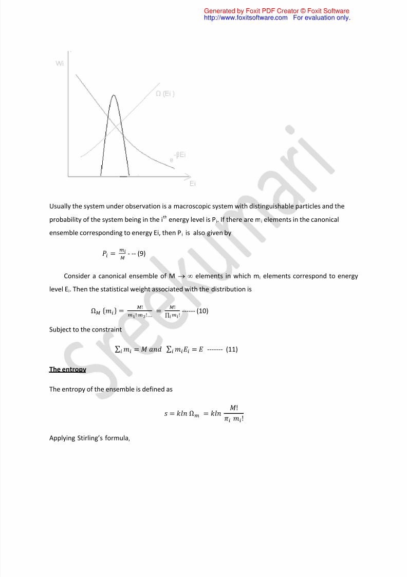
Usually the system under observation is a macroscopic system with distinguishable particles and the

probability of the system being in the ith

energy level is Pi. If there are mi elements in the canonical

ensemble corresponding to energy Ei, then Pi is also given by

= - -- (9)

Consider a canonical ensemble of M elements in which mi elements correspond to energy

level Ei. Then the statistical weight associated with the distribution is

Ω = !! !…. = !∏ ! ------ (10)

Subject to the constraint

∑ = ∑ = ------- (11)

The entropy

The entropy of the ensemble is defined as

= Ω = ! ! Applying Stirling’s formula,




= ln − − ln +

= ln − ln

The average entropy per element of the ensemble is

= = ln − 1 ln

= − ln = − ln

, = − ∑ ------- (12)

The energy Ei is a function of V & N. The partition function can be written as

= = + + ⋯ + + ⋯

Thus the partition function ‘Z’ is a function of V, N & b (Since energy Ei is in function of V & N). The terms

in the summation indicate how the ensemble is partitioned among various energy states.

The average value of any quantity R (Ei) is written as

= ()

Using this,

= =

.

= − 1

Or = − (ln) ------- (a)




From = − ∑ ln

we get = − ∑ ln

= − [– − l n ] = + E + l n

= + --- (14)

= 1

\ dS = k b dE – KE d b + k d(ln Z) --- (15)

Since Z = Z(b, V, N)

( ) = ( ) + ( ) + (ln )

= (,)

∴ (ln)

= å

× − = −

(ln) = å × −

& ( ) = å × − ∴ (ln ) = − å − å − å

., ln = − − −

\ = + − − −




= − −

If we write

= U

= − ∑ − ∑ --- (16)

= , + ,

+ , --- (17)

Comparing (16) and (17) We have

, = b = - -- (a)

(18) , = = − ∑ -- (b)

, = − = − − − − − ( )

Using b

=

= in eqn (14), we get

= + ln --- (d)

Or = +

Or – = − = , the Helmholtz free energy

ie, = − = − (, , )

= = − ln = − (ln)

b = 1 \ = − 1

= −




= = ln

= = −

Since = − , = exp (− )

1 = /

∴ () = / = /. /

() = ()/------ (19)]

Ideal gas in canonical ensemble

For an ideal Boltzmann gas consisting of N molecules of mass m, any arbitrary energy E of the system is

= 2 ,

= ∑ ∑

=

∑ ∏

The summation over discrete states can be replaced by integration over phase space

→ 1! … − − − ℎ

∴ = 1! ℎ ()

Z = ! ∫ / ∫ / … . ∫ /

Z =! ∫ /

This integral can be evaluated using the identify




= − +ln()

= −ln + 1

= − (/) – = −

∴ ¶ ¶ = − l n − ¶

¶

=

¶

¶

ln

∴ ¶

¶ ln =

∴ ¶ ¶ = − − ln

The entropy of the system in given by ∴ = −(¶ ¶ )V

, = ln + × p / p / × /

= ln + × 32

= ln

+ 3

2

, = ln 1 + 52

This equation is in agreement with Sakur – Tetrode equation




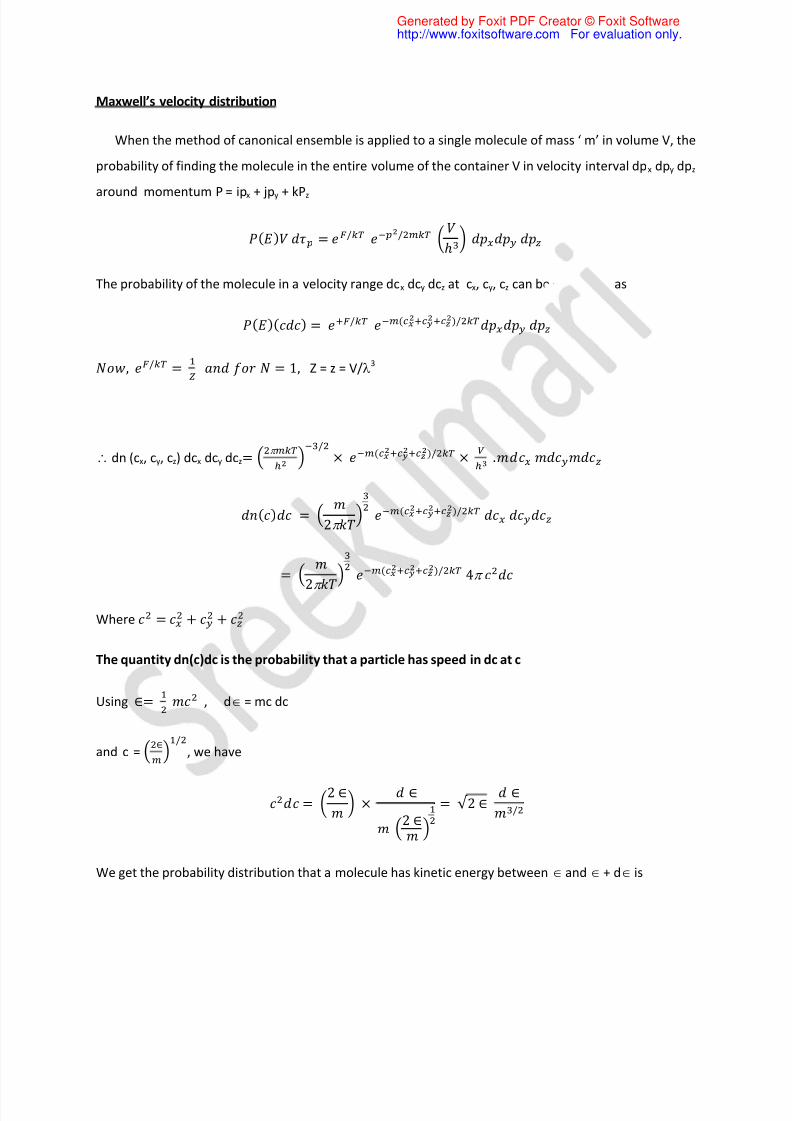
Maxwell’s velocity distribution

When the method of canonical ensemble is applied to a single molecule of mass ‘ m’ in volume V, the

probability of finding the molecule in the entire volume of the container V in velocity interval dpx dpy dpz

around momentum P = ipx + jpy + kPz

() = / / ℎ The probability of the molecule in a velocity range dcx dcy dcz at cx, cy, cz can be expressed as

()() = / ()/

, /

=

= 1,Z = z = V/

3

\ dn (cx, cy, cz) dcx dcy dcz= p / × ()/ × .

() = 2p ()/

= 2p

(

)/ 4p

Where = + +

The quantity dn(c)dc is the probability that a particle has speed in dc at c

Using ∈= , dÎ = mc dc

and c = ∈ /, we have

= 2 ∈ × ∈ 2 ∈ = √2 ∈ ∈/

We get the probability distribution that a molecule has kinetic energy between Î and Î + dÎ is




() = /2p √ 2p ∈/ × 4p × √2 ∈ ∈/

=2

√ p ∈

∈/

∈ ≡ ∈ ∈

Now ∈ is the product of two function – one an exponential decay function and another one

increasing withÎ. So dn(Î) has a peak where the two curves intersect as shown in figure

e-Î/kT is called Boltzanann factors and 2 ∈p /

is the density of states.

Equipartition of energy

Considering the case of a single particle, ie., N = 1, we have

= = −1 b = 32

For a single particle, total energy is kinetic.

\ H = where (P = P1, P2, P3)




Thus, each variable of the system like p i’s and qi’s contribute an average energy to the total energy

of the system if its Hamiltonian is expressed as a quadratic function of these variables.

Q: What is the total energy of a particle at temp T if the Hamiltonian of the system is H = ap2 + bx2

For example if H= ∑ +

the average energy due to is:

= ∫ / ∫ /

= ∫ /

∫

/

= − ∫ /∫ /

= − ln /

= −

ln p

/

= − ln p

= − p / × − 12 √ p / =

Similarly we can show for the term also

Thus each quadratic term in the expression for Hamiltonian contribute an energy

to the

average energy of the system. This theorem is known as equipartition theorem of energy.




Grand canonical ensemble

In microcanonical ensemble method, we had a totally isolated system defined by macroscopic

variables N, V, E. In canonical ensemble method, the constant energy constraint was relaxed and energy

was allowed to vary as the system exchanged energy with a reservoir.

But in several chemical processes, the number of particles of the system under observation

varies. In Quantum Mechanics also, the number of particles of the system under observation varies, as

particles can either be created or destroyed. Thus we need an ensemble method to deal with systems

where neither energy nor number of particles remain constant ie, the system under observation

exchanges both energy and particles with a reservoir. The ensemble of such a system is called grand

canonical ensemble. But the system under observation along with the reservoir again form an isolated

system with total energy and total number of particles conserved. Now, the macroscopic state of thesystem under observation is defined by (V,T,m) where m is the chemical potential per particle of the

system.

Thus = + and = + Now, D (, , , ) = D(, ) D(, )

The phase space dimension now depends on the number of particles in the ith

quantum state of the system. A particular quantum state of the system is represented by with

energy and number of particles . If is the probability of finding the system in the ith quantum

state with energy Then

(, )µ Dt [(-), (-)] ---- (1)

This is possible because the system under consideration will be in equilibrium when the

reservoir itself is in equilibrium as both are in contact and form an isolated system together.

The total number of microstates available to the composite system is very nearly equal to the

total number of microstates available to the reservoir itself because the system under consideration is

very small in comparison to the reservoir. ie, ≪ & << ≪ . Hence we can expand

ln Dt [(-), (-)] into a Taylor series in and abount = & = as




ln Dt [(-), (-)] = ln Dt (, ) - lnDt − lnDt ---- (2)

Now using substitution,

b = (lnDt ) −bm = (lnDt )

We have

ln Dt [(-), (-)] - ln Dt (, ) = -b+ bm + …….. (4)

Taking exponential,

Dt [(-), (-)]= Dt (, ) b (m )

But Dt (, ) is a constant independent of or . Thus equation (1) can be written as

(, ) = C b (m ) --------- (5)

Where C = BDt (, ) where B & C are constants independent of (, ). Such an ensemble with

probability distribution of form given by eqn(5) is called Grand canonical Ensemble and the

corresponding distribution is grand canonical distribution. The constant C of equation (5) can be

determined from the normalization condition.

( , ), = b (m ), = 1

\ = 1∑ b (m ),

\ ( , ) = b

m

---- (7)

Where

= exp−b − ,




---- (8)

is the grand canonical partition function. It is the sum of canonical partition function Z(N) for canonical

ensemble with different Ns with a weighing factor of . That is,

= b bm = b

bm ,

()bm

Thus the grand canonical ensemble can be thought of as made of a collection of canonical ensemble

with different values of N

= ()bm

ℎ () = b

Consider a grand canonical ensemble of

elements where

→ ∞. The state of each element is

characterized by the energy and number of particles ‘N’ in it. The statistical weight Ωof the

ensemble associated with a particular macrostate is

Ω = !∏ ∏ !

subject to the constraints

= ,

= ,, = ,

Where is the total number of particles in the ensemble.




Thus

= = b ()∑ b (),

Then, the entropy is defined as

= − ln

− ln b () ,

= − , b − bm + ,

= −b − mb + ln = 1, Taking a small variation in entropy,

ds = kbdÎ - kmbdN + kd ln

(here b is held constant as entropy can be taken to be a function of maximum three variables.

Here () and (V)

\ (V)

\

dln (ln )

,ln = 1 å b (m ) = 1 b (m )

, × −b




\ = b Î − mb − b ,m , \

, =

1 , = −m

, = = −1 ,

\ = −1

,

= b − bm + lnUsing = U and b =

S = − m + ln

\ = − m + ln Putting - kT ln

=

Ω=

− − , where

Ω is called the grand canonical potential

\ = /

But from 2nd law of thermodynamics, we have

= + − Ω = − − = −

From this equation

S = − Ω and N = − m Ω

= , 1 = In general, () = b (m ) = m /




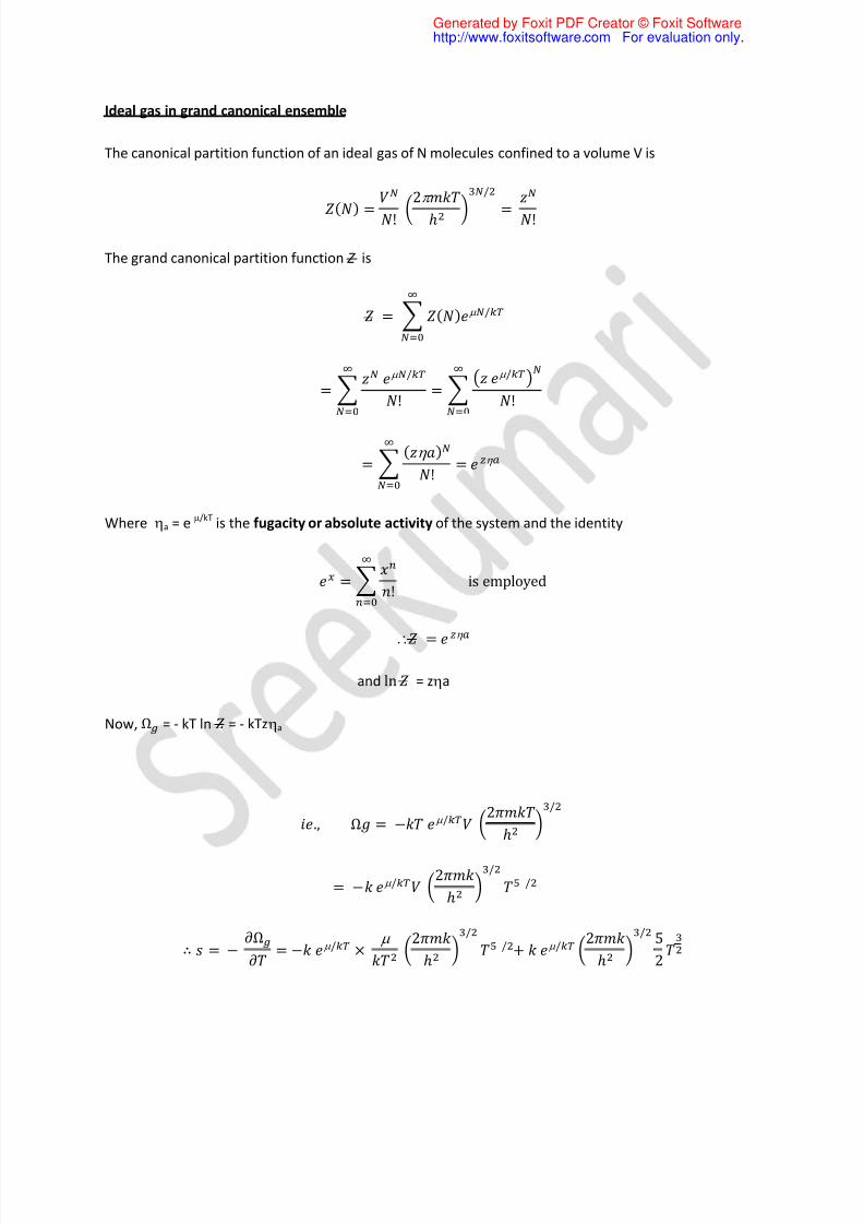
Ideal gas in grand canonical ensemble

The canonical partition function of an ideal gas of N molecules confined to a volume V is

() =

! 2p

ℎ /

=

! The grand canonical partition function Z is

= ()m /

= m /

!= m /

!

= ( )! =

Where a = em/kT

is the fugacity or absolute activity of the system and the identity

= ! is employed

\ =

and ln = za

Now, Ω = - kT ln = - kTza

., Ω = − m / 2

ℎ /

= − m / 2ℎ / /

∴ = − Ω = − m / × m 2ℎ / /+ m / 2ℎ / 52




= m / 2ℎ / 52 − m

This is again another form of Sakur- Tetrode equation for the entropy of an ideal gas

= − Ω = . m / × 1 × . 2ℎ /

= − Ω

From the above equation,

m = 1 \ m = −ln 1

, m = −ln = ln

Where n =

is the concentration of the particles and

=

is the quantum concentration or the

concentration associated with a single particle enclosed in a cube of side . Thus m increases with n and

a is directly proportional to n

Since Ω = - PV , P = - Ω

P = −kT em/ 2πmkTh / = kTNV

Thus PV = is the ideal gas law

Photons

Photons are spin -1 particles and hence they are Bosons and obey BE statistics. The energy of a




photon of frequency g is E= hg and the associated momentum is = g . The number of quantum state

between momentum range p and p + dp isDt

ie, The density of states between p and p + dp is

g(p) dp = 4ppdp

Since the photons have two independent directions of polarization,

g(p)dp = 2 ( 4pVh pdp) = 8pVh hgc hdgc ie, g(g)dg = gdg is the number of quantum states lying in this frequency range between g andg+ dg T hus the number of photons lying in this frequency range is

g(g)dg x (g ) where (g ) is the B-E probability distribution function

\dn = g(g)dg x (g ) = 8πVC gdg x 1e(µb) − 1where for photons E = hg and = 0

\

dn = 8πVc g

dg

1eg

/ − 1

Thus the total energy of photon in this range is

dn x hg = hgdg × g/ Thus energy density for this range in g = ∈ = gg × g/ This is Planck’s radiation law for photons

For hg << kT ie, for low frequency or high wave length region,

eg/ = 1 + g \ eg/ − 1 = g

\ g = pg × gg = p g

g → This is Rayleigh – Jeans law




For hg >> kT , ehg/kT

>> 1, one can be neglected compared to ehg/kT

\ g = pg g/ g → This is Wein’s law

The Total energy density is

UV = u(g, T)dg = 8phc

gdgeg/ − 1

Puttingg = x, g =

, dg = dx

\

UV = 8p

hc kTh

x

dxe − 1

The integral evaluates to

\UV = 8phC kTh × π15 = 8πkT15Ch

or = where b =

This is Stefan – Boltzmann radiation law


UnitII Canonical and grand canonical ensembles

Documents

Transcript of UnitII Canonical and grand canonical ensembles