1

Lecture 5Lecture 5

•The grand canonical ensemble.

•Density and energy fluctuations in the grand

canonical ensemble: correspondence with other

ensembles.

•Fermi-Dirac statistics.

•Classical limit.

•Bose-Einstein statistics.

2

The grand canonical ensemble. The grand canonical ensemble.

We want the probability dwdwss(N(Nss)) of a state of the subsystem

in which the subsystem contains NNss particles and is found in

the element ddss(N(Nss)) of its phase space. The notation ddss(N(Nss))

reminds us that the nature of phase space ss changes with NNss:

the number of dimensions will change.

(s)

Rest ( r ) or heatreservoir

Subsystem

Total system (t)

We now consider a subsystem subsystem ss which can exchange particles and energy with the heat reservoir rr, the total total systemsystem tt being represented by a microcanonical ensemble microcanonical ensemble with constant energy and constant number of particles.with constant energy and constant number of particles.

3

We do not care about the state of the remainder of the system provided only that

(5.1) NNN ,EEE trstrs

Then, by analogy with the treatment of the canonical ensemble,

(5.2) )N-(N)(Nd C)(Ndw strssss

dw Ce d NsE E N N

s sr t s t s ( ; ) ( ) (5.3)

or

We expend r in a power series:

sssttr

st

ttrs

t

ttrttrststr

NENE

NN

NEE

E

NENENNEE

),(

...`

),(),(),();(

(5.4)

recalling that 1

E NV N E V, ,

; - (5.5)

4

(5.5)

(5.6)

(5.7)

(5.8)

Dropping the subscript s, we have

)N(dAe)N(dw kT/)EN( where A is normalization constant. Writing by convention

kT/eA we have

)N(d)N()N(de)N(dw kT/)EN(

kT/)EN(e)N( where

is the grand canonical ensemblegrand canonical ensemble.

If several molecular species are present, NN is replaced by

NNiiii.. The quantity is called the grand potential. grand potential.

5

Grand partition function Grand partition function

(5.9)

(5.10)

The normalization is

1)()()( /)(

N

kTEN

N

NdeNdN

We define the grand partition grand partition functionfunction

Z e e e d NkT N kT E kT

N

/ / / ( ) (classical)

(quantum) eN i

kTEN iN /)( ,Z (5.11)

6

Connection with thermodynamic functions Proceeding at the same way that in the case of the canonical ensemble, we get for the entropy

ln ln ( , ) ( ) / N E N E kT (5.12)

FNE (5.13)or

G, where G is the Gibbs free energypVEG (5.14)

VdppdVdd-dEdG (5.15)

Now bydNpdVddE (5.16)

whence dNVdpd-dG (5.17)

Let us prove now that =

N

7

(5.18)

,pN

G

Now G G may be written as NN times a function of pp and along. Both p p and are intrinsic variables and do not change value when two identical systems are combined in one. For fixed p p and , GG is proportional to N N and consequently

(5.19)),p(NG g

where gg is the Gibbs free energy per particleGibbs free energy per particle. In this case, we have

(5.20)

),(pN

G

,p

g

whence

),p(NG (5.21)

Then from (5.13)

pVFGN (5.22)FNE (5.13)

8

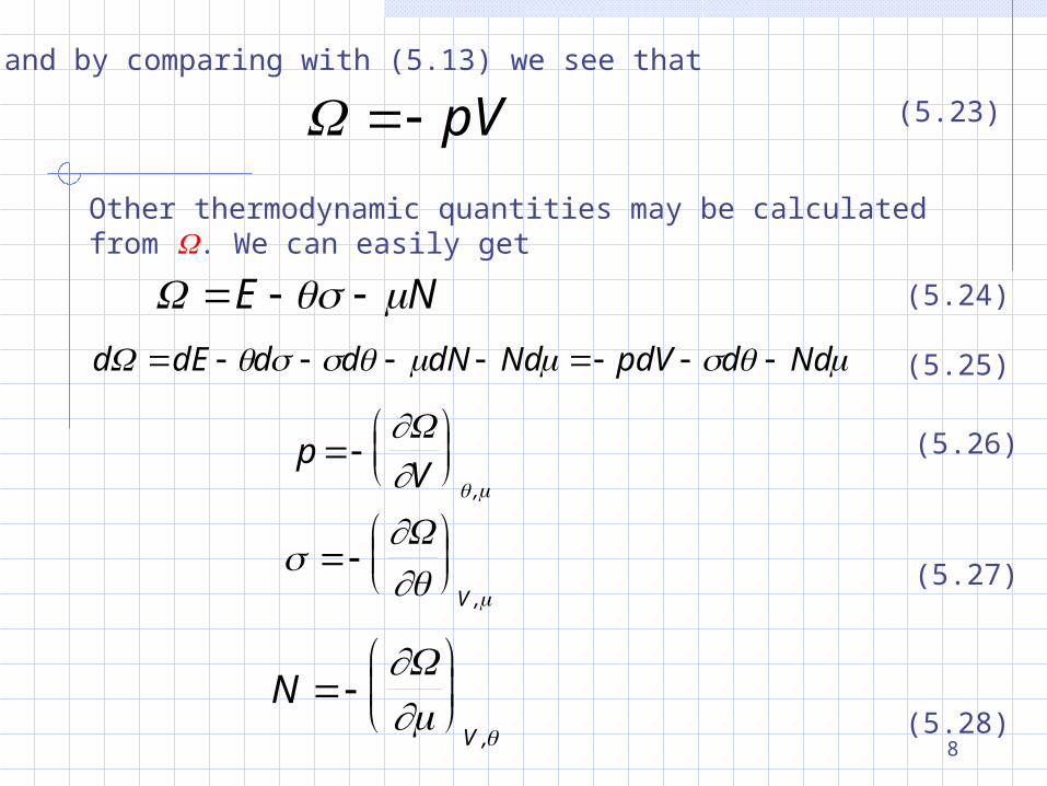
and by comparing with (5.13) we see that

pV (5.23)

Other thermodynamic quantities may be calculated from . We can easily get

NE (5.24)

NddpdVNddNdddEd (5.25)

pV

,

(5.26)

V ,(5.27)

NV

, (5.28)

9

Fermi-statistics and Bose StatisticsFermi-statistics and Bose StatisticsFermi-statistics and Bose StatisticsFermi-statistics and Bose Statistics

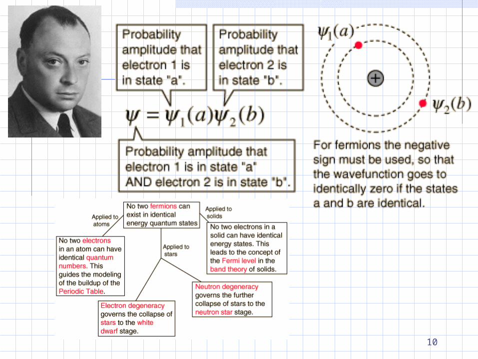
The occupation numbers, or number of particles in each one-particle state are strongly restricted by a general principle of quantum mechanics. The wave function of a system of identical particles must be either symmetrical (Bose) or antisymmetrical (Fermi) in permutation of a particle of the particle coordinates (including spin). It means that there can be only the following two cases: for Fermi-Dirac Distribution (Fermi-statistics) n=0 or 1

for Bose-Einstein Distribution (Bose-statistics) n=0,1,2,3......

The differences between the two cases are determined by the nature of particle. Particles which follow Fermi-statistics are called Fermi-particles (Fermions) and those which follow Bose-statistics are called Bose- particles (Bosones).

Electrons, positrons, protons and neutrons are Fermi-particles, whereas photons are Bosons. Fermion has a spin 1/2 and boson has integral spin. Let us consider this two types of statistics consequently.

10

11

There are two possible outcomes: If the result confirms the hypothesis, then you've made a measurement. If the result is contrary to the hypothesis, then you've made a discovery.   

Born: 8 Aug 1902 in Bristol, England

Died: 20 Oct 1984 in Tallahassee, Florida,

USA

Enrico FermiPhysicist

1901 - 1954

Fermi-Dirac Distribution Fermi-Dirac Distribution

12

Fermi-Dirac Fermi-Dirac DistributionDistribution Fermi-Dirac Fermi-Dirac DistributionDistribution

As the particles are assumed to be non-interacting it is convenient to discuss the system in terms of the energy states ii

of one particle in a volume VV. We specify the system

by specifying the number of particles nnii , occupying the

eigenstate ii . We classify ii in such way that i i denotes a

single state, not the set of degenerate states which may have the same energy.On the above model the Pauli principle allows only the values nnii==1,01,0. This is, of course, just the elementary statement of the Pauli principle: a given state may not be occupied by more than one identical particle.The partition function of the system is

We consider a system of identical independent non-interacting particles sharing a common volume and obeying antisymmetrical statistics: that is, the spin 1/2 and therefore, according to the Pauli principle, the total wave function is antisymmetrical on interchange of any two particles.

13

Z e n

n

i i

i

{ }

(5.29)

subject to . We note that the in the exponent runs over all one-particle states of the system; {n{n

ii}} represents nn allowed set of values of the nnii ; and runs over all such sets. Each nni i

may be 0 or 1. 0 or 1. { }ni

n Nii

Let us consider as an example a system with two states 1 and 2. The upper sum reads

e n n ( )1 1 2 2 (5.30)

)(

)()()(

e

eeeZ21

212121

11

100100

(5.31)

the other sum reads

but we have not included the requirement n1+n2=N. If we take N=1, we have

Z e e 1 2 (5.32)

14

For a system with many states and many particles it is difficult analytically to take care of the condition ni=N. It is more convenient to work with grand canonical ensemble. We have for the grand partition function

Z e en n

n

n

n

i i i

i

i i

i

( )

{ }

( )

{ }

(5.33)

so that

Z e i i

i

n

in

( )

{ }(5.34)

A simple consideration shows that we may reverse the order of the and in (5.34). We note that the significance of the changes entirely, from {ni}=0,1. Every term, which occurs, for one order will occur for the other order

Z

e xi i

i

i

i

n

ni

n

ni

( )

, ,0 1 0 1

(5.35)

x eii ( ) (5.36)

where

15

Now from the definition of the grand partition function

Z e e N E

N

( ) (5.37)

we have

kT kT x

i

i

i

n

nii

i

ln lnZ (5.38)

(5.39) in

n

kT xi

i

i

lnwhere

For ni restricted to 0,1, we have

(5.40) )xln(kT ii 1Now

NV

i

i

,

(5.41)

16

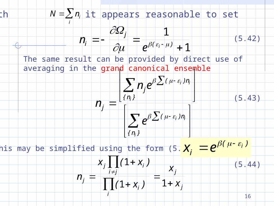
N nii

with it appears reasonable to set

nei

j

i

1

1( )(5.42)

The same result can be provided by direct use of averaging in the grand canonical ensemble

This may be simplified using the form (5.36):

n

n e

ej

jn

n

n

n

i i

i

i i

i

( )

{ }

( )

{ }

(5.43)

n

x x

x

x

xj

j ii j

ii

j

j

( )

( )

1

1 1

(5.44)

x eii ( )

17

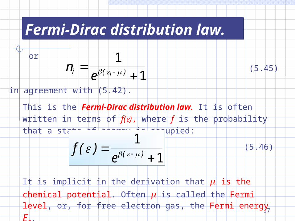
Fermi-Dirac distribution law. Fermi-Dirac distribution law.

or

nei i

1

1 ( ) (5.45)

in agreement with (5.42).

This is the Fermi-Dirac distribution law. It is often written in terms of f(), where f is the probability that a state of energy is occupied:

fe

( ) ( )

1

1f

e( ) ( )

1

1(5.46)

It is implicit in the derivation that is the chemical potential.

Often is called the Fermi level, or, for free electron gas, the

Fermi energy EF.

18

Classical limitClassical limit

For sufficiently large we will have (-)/kT>>1, and in this limit

kT/)(e)f( (5.47)

This is just the Boltzmann distribution. The high-energy tail of the Fermi-Dirac distribution is similar to the Boltzmann distribution. The condition for the approximate validity of the Boltzmann distribution for all energies 0 is that

1 kT/e (5.48)

19

Bose-Einstein Bose-Einstein DistributionDistributionBose-Einstein Bose-Einstein DistributionDistribution

20

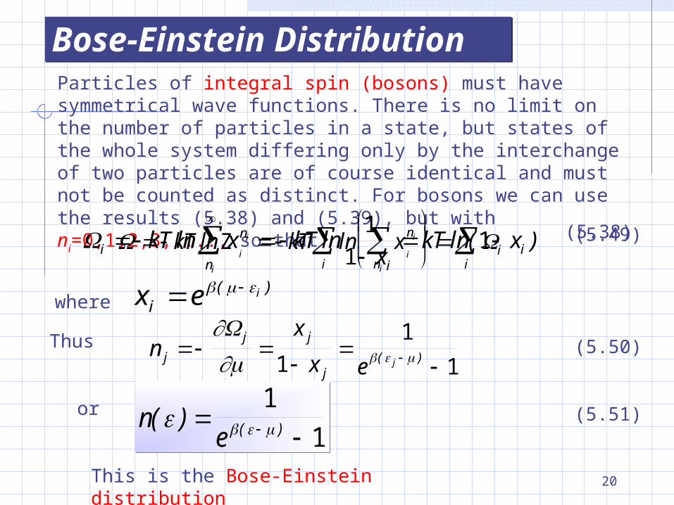
Bose-Einstein DistributionBose-Einstein DistributionParticles of integral spin (bosons) must have symmetrical wave functions. There is no limit on the number of particles in a state, but states of the whole system differing only by the interchange of two particles are of course identical and must not be counted as distinct. For bosons we can use the results (5.38) and (5.39), but with ni=0,1,2,3,...., so that

x eii ( )

where

in

n iikT x kT

xkT x

i

i

i

ln ln ln( )1

11 (5.49)

Thus nx

x ej

j j

jj

1

1

1( )(5.50)

or

This is the Bose-Einstein distribution

ne

( ) ( )

1

1n

e( ) ( )

1

1(5.51)

kT kT x

i

i

i

n

nii

i

ln lnZ (5.38)

21

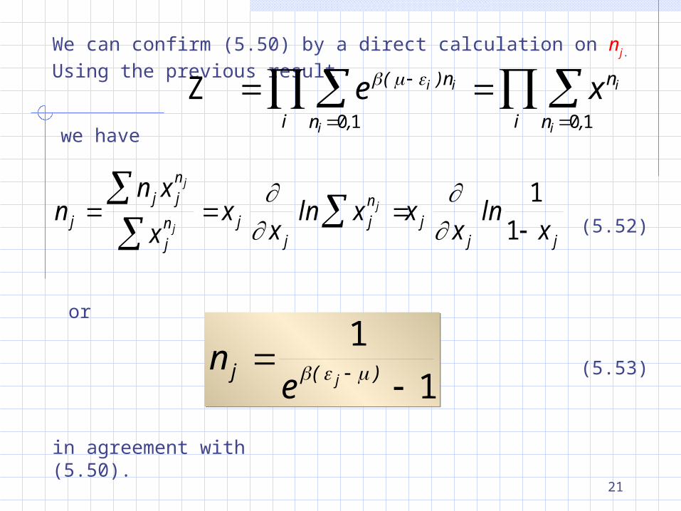
We can confirm (5.50) by a direct calculation on nj. Using the previous result

Z

e xi i

i

i

i

n

ni

n

ni

( )

, ,0 1 0 1we have

or

in agreement with (5.50).

nn x

xx x x

xj

j jn

jn j

jjn

jj j

j

j

j

x xln ln

1

1 (5.52)

ne

j j

1

1 ( )n

ej j

1

1 ( ) (5.53)