Unforced Surface Air Temperature Variability and Its Contrasting Relationshipwith the Anomalous TOA Energy Flux at Local and Global Spatial Scales*

PATRICK T. BROWN AND WENHONG LI

Earth and Ocean Sciences, Nicholas School of the Environment, Duke University, Durham, North Carolina

JONATHAN H. JIANG AND HUI SU

Jet Propulsion Laboratory, California Institute of Technology, Pasadena, California

(Manuscript received 29 May 2015, in final form 6 November 2015)

ABSTRACT

Unforced global mean surface air temperature (T) is stable in the long term primarily because warm T

anomalies are associated with enhanced outgoing longwave radiation ([LW) to space and thus a negative net

radiative energy flux (N, positive downward) at the top of the atmosphere (TOA). However, it is shown here

that, with the exception of high latitudinal and specific continental regions, warm unforced surface air tem-

perature anomalies at the local spatial scale [T(u, f), where (u, f)5 (latitude, longitude)] tend to be associated

with anomalously positive N(u, f). It is revealed that this occurs mainly because warm T(u, f) anomalies are

accompanied by anomalously low surface albedo near sea ice margins and over high altitudes, low cloud albedo

overmuchof themiddle and low latitudes, and a largewater vapor greenhouse effect over the deep Indo-Pacific.

It is shown here that the negativeN versus T relationship arises because warm T anomalies are associated

with large divergence of atmospheric energy transport over the tropical Pacific [where theN(u,f) versusT(u,f)

relationship tends to be positive] and convergence of atmospheric energy transport at high latitudes [where

the N(u, f) versus T(u, f) relationship tends to be negative]. Additionally, the characteristic surface tem-

perature pattern contains anomalously cool regions where a positive localN(u, f) versus T(u, f) relationship

helps induce negative N. Finally, large-scale atmospheric circulation changes play a critical role in the pro-

duction of the negative N versus T relationship as they drive cloud reduction and atmospheric drying over

large portions of the tropics and subtropics, which allows for greatly enhanced [LW.

1. Introduction

Changes in surface air temperature (T) can be caused by

external radiative forcings that imposeanet radiative energy

flux (N, positive down) at the top of the atmosphere (TOA):

N5YSW2[SW2[LW, (1)

where SW represents shortwave (solar) radiation at the

TOA, LW represents longwave (terrestrial) radiation at

the TOA, and the arrows represent the direction of the

flux. Additionally, T experiences unforced variability

that originates from the internal dynamics of the climate

system (Brown et al. 2014a; Hasselmann 1976; Hawkins

and Sutton 2009; Palmer and McNeall 2014). Unforced

variability in global mean T (T) has generated great

scientific and public interest as it has the ability to either

enhance or obscure externally forced signals such as the

long-term warming due to increased greenhouse gas

concentrations (Brown et al. 2015). Much work on the

causes of unforced T variability has focused on changes

in the net heat flux between the ocean and atmosphere

(Chen and Tung 2014; Drijfhout et al. 2014; England

et al. 2014; Meehl et al. 2013). However, it is also rec-

ognized that unforced variability inN, due to changes in

clouds in particular, can enhance the magnitude and

persistence of unforced T variability locally (Bellomo

et al. 2014, 2015; Evan et al. 2013; Trzaska et al. 2007).

Therefore, there has been substantial interest in the

* Supplemental information related to this paper is available at

the Journals Online website: http://dx.doi.org/10.1175/JCLI-D-15-

0384.s1.

Corresponding author address: Patrick T. Brown, Earth and

Ocean Sciences, Nicholas School of the Environment, Duke Uni-

versity, 5120K Environment Hall, 9 Circuit Drive, Durham, NC

27708.

E-mail: patrick.brown@duke.edu

1 FEBRUARY 2016 BROWN ET AL . 925

DOI: 10.1175/JCLI-D-15-0384.1

� 2016 American Meteorological Society

relationship between T and N in the context of un-

perturbed climate variability (Allan et al. 2014; Brown

et al. 2014a; Kato 2009; Loeb et al. 2012; Palmer and

McNeall 2014; Smith et al. 2015; Trenberth et al. 2014)

as this relationship may have implications for the mag-

nitude and persistence of unforced T variability.

When the climate system is unperturbed by external ra-

diative forcings, it is expected thatT wouldbe stable on long

time scales predominantly because of the Planck response,

or the direct blackbody radiative response to a uniform

temperature change of the surface and the atmosphere

(Bony et al. 2006;Dessler 2013;Hallberg and Inamdar 1993;

Ingram 2013). In the global mean sense, the Planck re-

sponse suggests that positive T anomalies tend to be asso-

ciated with enhanced[LW,whichwould cause negativeN,

and thus an eventual return of T to its equilibrium

value (Brown et al. 2014a; Dessler 2013; Koumoutsaris

2013; Trenberth et al. 2015). Indeed, both satellite obser-

vations and atmosphere–ocean general circulation models

(AOGCMs) show this negative N versus T global mean

relationship for interannual variability (Fig. 1a).

It may be tempting to suppose that this negative N

versus T global relationship should hold at the local

spatial scale as well, but it was recently pointed out

that the N(u, f) versus T(u, f) relationship [where

(u, f) 5 (latitude, longitude)] is in fact positive in

observations over much of Earth (Trenberth et al.

2015). Indeed, the same observations and AOGCMs

that demonstrate the negative N versus T relationship

(Fig. 1a) indicate that the N(u, f) versus T(u, f) re-

lationship tends to be positive over most of the surface

of the planet (Figs. 1b–d). The underlying reasons for

the spatial distribution of the N(u, f) versus T(u, f)

relationship as well as the cause of the relationship’s

sign reversal at the global scale are the primary topics

of investigation in this study. Elucidating these re-

lationships will improve our physical understanding

of unforced T variability and may improve efforts

to model climate variability on both local and global

scales.

2. Data, preprocessing, and definitions

a. AOGCM data

We focus on the relationship between unforced

anomalous annual mean T and unforced anomalous

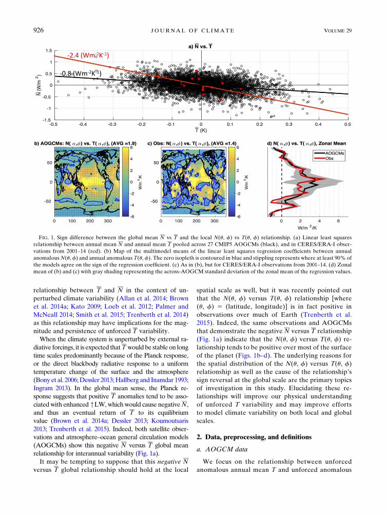
FIG. 1. Sign difference between the global mean N vs T and the local N(u, f) vs T(u, f) relationship. (a) Linear least squares

relationship between annual mean N and annual mean T pooled across 27 CMIP5 AOGCMs (black), and in CERES/ERA-I obser-

vations from 2001–14 (red). (b) Map of the multimodel means of the linear least squares regression coefficients between annual

anomalousN(u, f) and annual anomalous T(u, f). The zero isopleth is contoured in blue and stippling represents where at least 90% of

the models agree on the sign of the regression coefficient. (c) As in (b), but for CERES/ERA-I observations from 2001–14. (d) Zonal

mean of (b) and (c) with gray shading representing the across-AOGCM standard deviation of the zonal mean of the regression values.

926 JOURNAL OF CL IMATE VOLUME 29

annual mean energy fluxes in 27 AOGCMs that par-

ticipated in phase 5 of the Coupled Model In-

tercomparison Project (CMIP5; Taylor et al. 2012).

Details on the AOGCMs used in this study can be

found in Table S1 in the supplementary material. We

utilized unforced preindustrial control runs, which

included no external radiative forcings, and thus all

variability emerged spontaneously from the internal

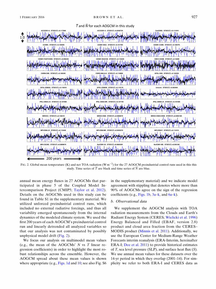
dynamics of the modeled climate system. We used the

first 200 years of each AOGCM’s preindustrial control

run and linearly detrended all analyzed variables so

that our analysis was not contaminated by possibly

unphysical model drift (Fig. 2).

We focus our analysis on multimodel mean values

(e.g., the mean of the AOGCMs’ N vs T linear re-

gression coefficients) in order to highlight the most ro-

bust relationships across the ensemble. However, the

AOGCM spread about these mean values is shown

where appropriate (e.g., Figs. 1d and 10; see also Fig. S6

in the supplementary material) and we indicate model

agreement with stippling that denotes where more than

90% of AOGCMs agree on the sign of the regression

coefficients (e.g., Figs. 1b, 3a–k, and 6a–k).

b. Observational data

We supplement the AOGCM analysis with TOA

radiation measurements from the Clouds and Earth’s

Radiant Energy System (CERES; Wielicki et al. 1996)

Energy Balanced and Filled (EBAF, version 2.8)

product and cloud area fraction from the CERES–

MODIS product (Minnis et al. 2011). Additionally, we

use the European Center for Medium-Range Weather

Forecasts interim reanalysis (ERA-Interim, hereinafter

ERA-I; Dee et al. 2011) to provide historical estimates

of T, sea level pressure (SLP), and surface heat flux (S).

We use annual mean values for these datasets over the

14-yr period in which they overlap (2001–14). For sim-

plicity we refer to both ERA-I and CERES data as

FIG. 2. Global mean temperature (K) and net TOA radiation (Wm22) for the 27 AOGCM preindustrial control runs used in this this

study. Time series of T are black and time series of N are blue.

1 FEBRUARY 2016 BROWN ET AL . 927

observations even though ERA-I output represents

observations assimilated into a weather forecast model.

We linearly detrend all of the observations prior to

further analysis. It should be noted that the historical

record contains a combination of both forced and un-

forced variability; these are difficult to disentangle but

over the relatively short time period of investigation

(2001–14) unforced variability accounts for a substantial

majority of the observed variation (Dessler 2010; Trenberth

et al. 2010).

The purpose of this manuscript is to use both AOGCMs

and observations to gain physical insight on the cova-

riability between N and T. Therefore, it is not our in-

tent to rigorously compare AOGCMs to observations

in order to assess model performance. Nevertheless,

AOGCMs are known to struggle with the simulation of

clouds, and thus it is useful to keep in mind that there are

some large differences between AOGCM-modeled and

observed cloud climatologies (Fig. S1 in the supplemen-

tary material). See also Dolinar et al. (2015) for further

discussion.

c. Definitions

1) LOCAL AND GLOBAL SPATIAL SCALE

We bilinearly interpolate all variables (a) from both

AOGCM and observational datasets to a common

2.58 3 2.58 latitude–longitude [(u, f)] grid. Global mean

values, denoted by an overbar, are calculated as

a51

A�M

i

ai[a(u,f)]

i, (2)

where the i subscript indicates the ith value of a total of

M, which is weighed by the grid box area ai and nor-

malized by the total Earth surface area A.

2) COMPONENTS OF N

To gain insight into the underlying physics governing

N variability, we follow previous studies (Ramanathan

et al. 1989) to decompose N into four linearly additive

components:

ClearSW

5 [YSW2[SWclear_sky

] , (3)

ClearLW

5 [2[LWclear_sky

] , (4)

CRESW

5 [YSW2[SWall_sky

]2 [YSW2[SWclear_sky

]

5[SWclear_sky

2[SWall_sky

, and

(5)

CRELW

5 [2[LWall_sky

]2 [2[LWclear_sky

]

5[LWclear_sky

2[LWall_sky

, (6)

where ClearSW, ClearLW, CRESW, and CRELW repre-

sent the anomalous clear-sky shortwave, anomalous

clear-sky longwave, anomalous cloud radiative effect

(CRE) shortwave, and CRE longwave components, re-

spectively, at the TOA (all positive downward). We also

investigate the net impact of clouds using

CRE5CRESW

1CRELW

. (7)

The CRE is a measure of the impact of cloud radiative

properties and cloud fraction on the TOA radiation

budget relative to a cloudless atmosphere (Ramanathan

et al. 1989). Thus, a change in the CRE with T is not a

pure measure of cloud feedback since a change in the

CRE can occur because of a change in clouds or a

change in the clear-sky radiation budget (Soden et al.

2004). This makes it difficult to isolate the effect of

clouds onN over regions with large changes in the clear-

sky energy budget. Nevertheless, decomposing N using

Eqs. (3)–(7) provides some physical insight that would

not be available otherwise. In future work it may be

valuable to investigate the components of N using dif-

ferent methods such as the partial radiative perturbation

technique (Donohoe and Battisti 2011).

3) SURFACE AND ATMOSPHERIC ENERGY FLUXES

The net anomalous upward surface heat flux (S) is

S5[LE1[SH1 [[SWS2YSW

S]1 [[LW

S2YLW

S] ,

(8)

where LE is the anomalous latent heat flux, SH is the

anomalous sensible heat flux, SWS is the anomalous

shortwave radiation flux, and LWS is the anomalous

longwave radiation flux all defined at Earth’s surface

under all-sky conditions.

We follow (Trenberth et al. 2002a,b) to define an es-

timate of the convergence of the vertically integrated

atmospheric energy transport (AET):

2= �AET(u,f)521[N(u,f)1 S(u,f)] . (9)

For observations, both S(u, f) and N(u, f) in Eq. (9)

came from ERA-I [rather than using N(u, f) from

CERES] so that potentially disparate datasets were not

mixed. This approximation ignores any atmospheric

storage of heat, which was assumed to be small.

4) LINEAR REGRESSION RELATIONSHIPS

In the sections below we will make use of the following

notation to denote a variety of different linear least squares

regression relationships between climatic variables (a) and

T both on the local [T(u, f)] and global [T] scales.

928 JOURNAL OF CL IMATE VOLUME 29

The regression coefficient between any global mean

variable a and T is denoted as

ga5

Da

DT. (10)

The corresponding regression coefficient at the local

spatial scale is denoted as

ga(u,f)5

D[a(u,f)]

D[T(u,f)]. (11)

Note that the global mean of the regression coefficients

calculated on the local scale [ga(u, f)] is not the same

quantity as the regression coefficient calculated on

global means [ga] as Fig. 1 demonstrates.

Finally, the linear relationship between a variable

defined at the local spatial scale and T is denoted as

za(u,f)5

D[a(u,f)]

DT. (12)

5) FEEDBACKS

We follow convention by referring to the linear re-

lationship between a TOA radiative flux anomaly and

a T anomaly as a ‘‘feedback’’ (Bellomo et al. 2015;

Colman and Power 2010; Dessler 2013; Koumoutsaris

2013; Trenberth et al. 2015). This language can give the

impression that we know the change in T is the cause

and the change in TOA flux is the effect. It is safe to

assume this direction of causality when an external

forcing is obviously responsible for the T change but

the direction of causality is more ambiguous in the

unforced climate state where all variability is sponta-

neously generated by the system itself. Undoubtedly

there are instances where changes in the TOA flux

(e.g., atmospheric circulation induced changes in

clouds over land) lead to the T anomaly (Trenberth

and Shea 2005). Therefore, we caution that we use the

term feedback to be consistent with other contempo-

rary work on this subject but we do not wish to convey

that the direction of causality is necessarily known in

all cases.

3. The geographic distribution of the gN(u, f)relationship

We first investigate the local relationships between N

and T [gN(u, f); Eq. (11)] with the intent of uncovering

the physical processes underlying these relationships as

well as how these physical processes differ by geographic

location. Figure 3 maps ga(u, f) for a number of

variables in both AOGCMs (Figs. 3a–k) and observa-

tions (Fig. 3l–v). Note that gClear LW(u, f) (Figs. 3e,p) is

affected by the lapse rate feedback, the water vapor

feedback, and the Planck response (Colman and Power

2010; Crook et al. 2011), but overmost of Earth’s surface

the Planck response dominates this component and

there is enhanced [LW(u, f) to space during elevated

T(u,f). [Note that[LWvia the Planck response is more

heavily influenced by tropospheric mean temperature

than by T itself but that T and tropospheric mean tem-

perature are positively correlated on these time scales

(Trenberth et al. 2015).] In the AOGCMs, the primary

exception to this enhanced[LW(u, f) withwarmT(u,f)

is over the Indo-Pacific warm pool where higher clima-

tological surface temperatures allow for a water vapor

response that is strong enough to overwhelm the Planck

response (Allan et al. 1999; Inamdar and Ramanathan

1994; Larson and Hartmann 2003; Pierrehumbert 1995;

Ramanathan and Collins 1991; Su et al. 2006). In this

region, anomalous warmth is also associated with en-

hanced convection and cloud fraction (Fig. 3k) but since

the shortwave (Fig. 3c) and longwave (Fig. 3f) CRE

components mostly cancel (Fig. 3i) (Kiehl 1994), it is the

water vapor feedback (Fig. 3e) that is primarily re-

sponsible for the positive gN(u, f) relationship there.

Note that the strength of the water vapor response also

depends on enhanced convection as moistening of the

middle and upper troposphere is crucial for its large

magnitude in this region (Hallberg and Inamdar 1993).

Observations tell a similar story except that

gClear LW(u, f) is negative over the central portion of the

Indo-Pacific warm pool (Fig. 3p). This disagreement

may be because satellites are only able to sample

ClearLW(u, f) in regions that are actually cloud-free

[unlike AOGCMs which calculate ClearLW(u, f) at all

grid points and at every time step regardless of the

simulated cloud cover]. A consequence of this is that the

ClearLW(u, f) measurement from satellites will dispro-

portionately represent the cloudless areas with less hu-

midity and less of a water vapor greenhouse effect.

Over most of the remainder of the surface, with the

exception of the subpolar latitudes, the positive gN(u, f)

relationship is due mostly to the gCRESW(u, f) compo-

nent (Figs. 3c,n) associated with a reduction in cloud

fraction (Figs. 3k,v) and an overall positive gCRE(u, f)

(Figs. 3i,t). This is consistent with the shortwave cloud

feedback that has been noted in regions characterized by

high-albedo, low-level stratiform clouds in particular

(Evan et al. 2013; Park et al. 2005). In these regions,

elevated T(u, f) is associated with increased convection

and destabilization of the boundary layer (Bellenger

et al. 2014) as well as a lack of sufficient increase in

evaporation to maintain the boundary layer cloudiness

1 FEBRUARY 2016 BROWN ET AL . 929

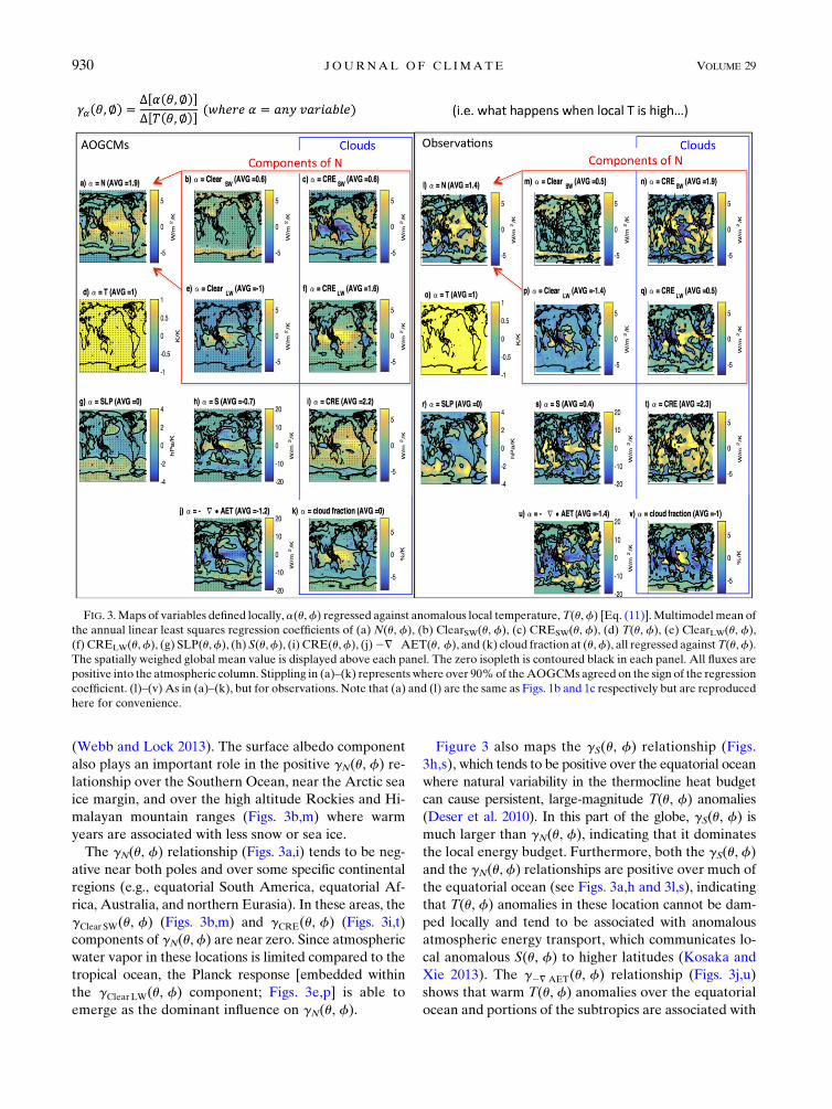
(Webb and Lock 2013). The surface albedo component

also plays an important role in the positive gN(u, f) re-

lationship over the Southern Ocean, near the Arctic sea

ice margin, and over the high altitude Rockies and Hi-

malayan mountain ranges (Figs. 3b,m) where warm

years are associated with less snow or sea ice.

The gN(u, f) relationship (Figs. 3a,i) tends to be neg-

ative near both poles and over some specific continental

regions (e.g., equatorial South America, equatorial Af-

rica, Australia, and northern Eurasia). In these areas, the

gClear SW(u, f) (Figs. 3b,m) and gCRE(u, f) (Figs. 3i,t)

components of gN(u, f) are near zero. Since atmospheric

water vapor in these locations is limited compared to the

tropical ocean, the Planck response [embedded within

the gClear LW(u, f) component; Figs. 3e,p] is able to

emerge as the dominant influence on gN(u, f).

Figure 3 also maps the gS(u, f) relationship (Figs.

3h,s), which tends to be positive over the equatorial ocean

where natural variability in the thermocline heat budget

can cause persistent, large-magnitude T(u, f) anomalies

(Deser et al. 2010). In this part of the globe, gS(u, f) is

much larger than gN(u, f), indicating that it dominates

the local energy budget. Furthermore, both the gS(u, f)

and the gN(u, f) relationships are positive over much of

the equatorial ocean (see Figs. 3a,h and 3l,s), indicating

that T(u, f) anomalies in these location cannot be dam-

ped locally and tend to be associated with anomalous

atmospheric energy transport, which communicates lo-

cal anomalous S(u, f) to higher latitudes (Kosaka and

Xie 2013). The g2=�AET(u, f) relationship (Figs. 3j,u)

shows that warm T(u, f) anomalies over the equatorial

ocean and portions of the subtropics are associated with

FIG. 3.Maps of variables defined locally, a(u,f) regressed against anomalous local temperature,T(u,f) [Eq. (11)].Multimodelmean of

the annual linear least squares regression coefficients of (a) N(u, f), (b) ClearSW(u, f), (c) CRESW(u, f), (d) T(u, f), (e) ClearLW(u, f),

(f) CRELW(u,f), (g) SLP(u,f), (h) S(u,f), (i) CRE(u,f), (j)2= �AET(u, f), and (k) cloud fraction at (u,f), all regressed againstT(u,f).

The spatially weighed global mean value is displayed above each panel. The zero isopleth is contoured black in each panel. All fluxes are

positive into the atmospheric column. Stippling in (a)–(k) represents where over 90%of theAOGCMsagreed on the sign of the regression

coefficient. (l)–(v) As in (a)–(k), but for observations. Note that (a) and (l) are the same as Figs. 1b and 1c respectively but are reproduced

here for convenience.

930 JOURNAL OF CL IMATE VOLUME 29

net anomalous horizontal export of energy while warm

T(u, f) anomalies over many continental and high-

latitude regions are associated with the net anomalous

horizontal import of energy from other locations.

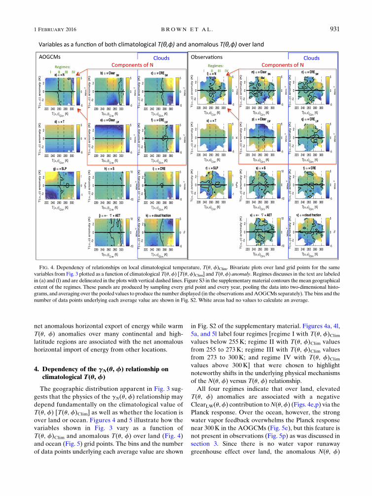
4. Dependency of the gN(u, f) relationship onclimatological T(u, f)

The geographic distribution apparent in Fig. 3 sug-

gests that the physics of the gN(u, f) relationship may

depend fundamentally on the climatological value of

T(u, f) [T(u, f)Clim] as well as whether the location is

over land or ocean. Figures 4 and 5 illustrate how the

variables shown in Fig. 3 vary as a function of

T(u, f)Clim and anomalous T(u, f) over land (Fig. 4)

and ocean (Fig. 5) grid points. The bins and the number

of data points underlying each average value are shown

in Fig. S2 of the supplementary material. Figures 4a, 4l,

5a, and 5l label four regimes [regime I with T(u, f)Climvalues below 255K; regime II with T(u, f)Clim values

from 255 to 273K; regime III with T(u, f)Clim values

from 273 to 300K; and regime IV with T(u, f)Climvalues above 300K] that were chosen to highlight

noteworthy shifts in the underlying physical mechanisms

of the N(u, f) versus T(u, f) relationship.

All four regimes indicate that over land, elevated

T(u, f) anomalies are associated with a negative

ClearLW(u,f) contribution toN(u,f) (Figs. 4e,p) via the

Planck response. Over the ocean, however, the strong

water vapor feedback overwhelms the Planck response

near 300K in the AOGCMs (Fig. 5e), but this feature is

not present in observations (Fig. 5p) as was discussed in

section 3. Since there is no water vapor runaway

greenhouse effect over land, the anomalous N(u, f)

FIG. 4. Dependency of relationships on local climatological temperature, T(u, f)Clim. Bivariate plots over land grid points for the same

variables from Fig. 3 plotted as a function of climatological T(u,f) [T(u,f)Clim] and T(u,f) anomaly. Regimes discusses in the text are labeled

in (a) and (l) and are delineated in the plots with vertical dashed lines. Figure S3 in the supplementarymaterial contours themean geographical

extent of the regimes. These panels are produced by sampling every grid point and every year, pooling the data into two-dimensional histo-

grams, and averaging over the pooled values to produce the number displayed (in the observations andAOGCMs separately). The bins and the

number of data points underlying each average value are shown in Fig. S2. White areas had no values to calculate an average.

1 FEBRUARY 2016 BROWN ET AL . 931

versus T(u,f) relationship (Figs. 4a,l) is governed by the

ability of the surface albedo (Figs. 4b,m) and CRE(u, f)

components (Figs. 4i,t) to overwhelm the ClearLW(u, f)

component.

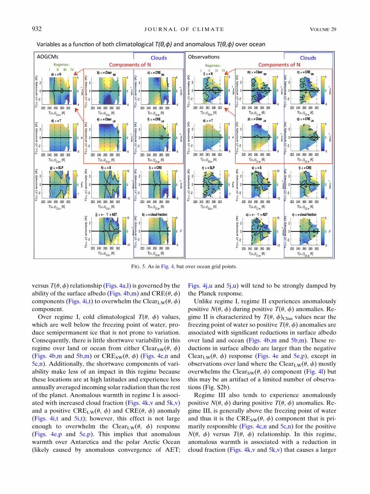
Over regime I, cold climatological T(u, f) values,

which are well below the freezing point of water, pro-

duce semipermanent ice that is not prone to variation.

Consequently, there is little shortwave variability in this

regime over land or ocean from either ClearSW(u, f)

(Figs. 4b,m and 5b,m) or CRESW(u, f) (Figs. 4c,n and

5c,n). Additionally, the shortwave components of vari-

ability make less of an impact in this regime because

these locations are at high latitudes and experience less

annually averaged incoming solar radiation than the rest

of the planet. Anomalous warmth in regime I is associ-

ated with increased cloud fraction (Figs. 4k,v and 5k,v)

and a positive CRELW(u, f) and CRE(u, f) anomaly

(Figs. 4i,t and 5i,t); however, this effect is not large

enough to overwhelm the ClearLW(u, f) response

(Figs. 4e,p and 5e,p). This implies that anomalous

warmth over Antarctica and the polar Arctic Ocean

(likely caused by anomalous convergence of AET;

Figs. 4j,u and 5j,u) will tend to be strongly damped by

the Planck response.

Unlike regime I, regime II experiences anomalously

positive N(u, f) during positive T(u, f) anomalies. Re-

gime II is characterized by T(u, f)Clim values near the

freezing point of water so positive T(u, f) anomalies are

associated with significant reductions in surface albedo

over land and ocean (Figs. 4b,m and 5b,m). These re-

ductions in surface albedo are larger than the negative

ClearLW(u, f) response (Figs. 4e and 5e,p), except in

observations over land where the ClearLW(u, f) mostly

overwhelms the ClearSW(u, f) component (Fig. 4l) but

this may be an artifact of a limited number of observa-

tions (Fig. S2b).

Regime III also tends to experience anomalously

positive N(u, f) during positive T(u, f) anomalies. Re-

gime III, is generally above the freezing point of water

and thus it is the CRESW(u, f) component that is pri-

marily responsible (Figs. 4c,n and 5c,n) for the positive

N(u, f) versus T(u, f) relationship. In this regime,

anomalous warmth is associated with a reduction in

cloud fraction (Figs. 4k,v and 5k,v) that causes a larger

FIG. 5. As in Fig. 4, but over ocean grid points.

932 JOURNAL OF CL IMATE VOLUME 29

reduction in cloud albedo (Figs. 4c,n and 5c,n) than

cloud greenhouse effect (Figs. 4f,q and 5f,q). The direction

of causality is particularly ambiguous in this regime

since reduced cloudiness leads to warmth (Trenberth

and Shea 2005).

Over land, where the water vapor supply is limited,

T(u, f) warmth in regime IV is associated with anoma-

lously negative N(u, f) (Figs. 4a,l). In this regime,

anomalous warmth is associated with decreased pre-

cipitation (Trenberth and Shea 2005) and cloud fraction

(Figs. 4k,v); however, because of longwave and short-

wave cancellation, the CRE(u, f) response is relatively

small (Figs. 4i,t). Also, since the T(u, f)clim value is well

above the freezing point of water, the ClearSW(u, f)

response is near zero. These factors allow the Planck

response (embedded in Figs. 4e and 4p) to dominate the

total response (Figs. 4a,l). Like regime I, regime IV over

land tends to be an area of AET convergence during

anomalous T(u, f) warmth (Figs. 4j,u).

5. The negative gN relationship

Having established some of the underlying physics

governing the geographic distribution of the local

N(u, f) versus T(u, f) relationship, we now turn our

attention to the problem of reconciling the mostly

positive local N(u, f) versus T(u, f) relationship

(Figs. 1b–d and 3a,l) with the negative N versus T (gN)

relationship (Fig. 1a). One possible way to square

these seemingly paradoxical results would be through

the specific spatial pattern of T(u, f) anomalies asso-

ciated with changes in T [i.e., zT(u, f); Eq. (12)]. Spe-

cifically, we showed in sections 3 and 4 that certain

locations on the surface of the planet are better able to

damp T(u, f) anomalies to space than others. For ex-

ample, anomalous warmth over Antarctica and the

polar Arctic Ocean will tend to be effectively damped

by the Planck response (Figs. 1b–d and 3a,l). There-

fore, if zT(u, f) was distributed such that most of the

anomalous warmth was in high-latitude regions char-

acterized by a negative gN(u, f) relationship, then the

apparent contradiction of Fig. 1a and Figs. 1b–d might

be resolved.

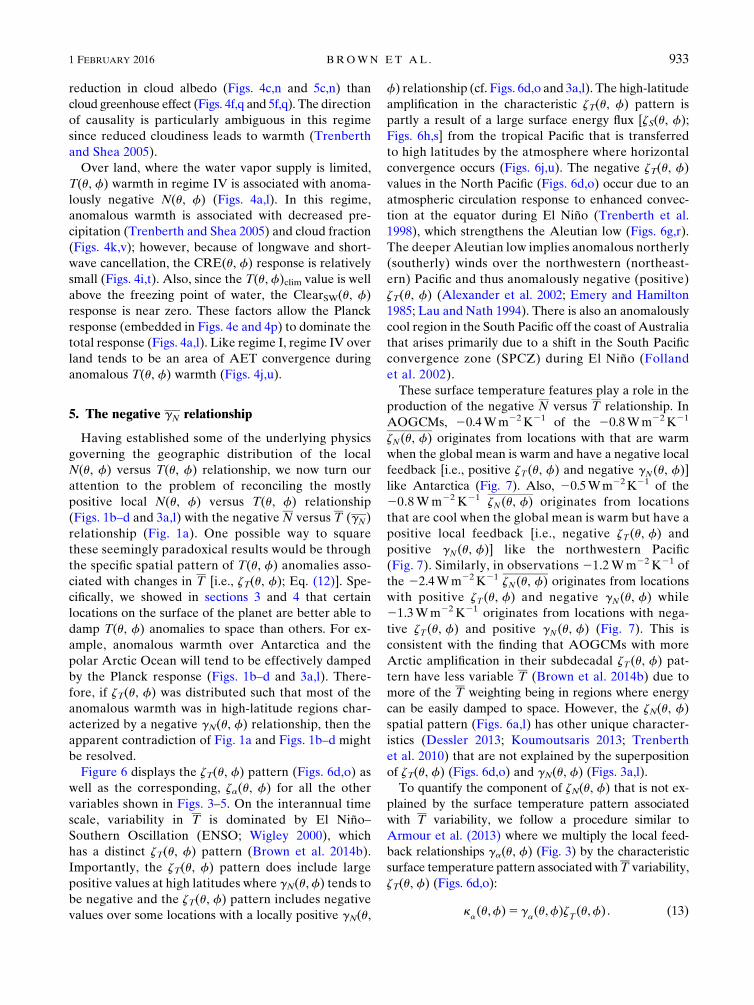
Figure 6 displays the zT(u, f) pattern (Figs. 6d,o) as

well as the corresponding, za(u, f) for all the other

variables shown in Figs. 3–5. On the interannual time

scale, variability in T is dominated by El Niño–Southern Oscillation (ENSO; Wigley 2000), which

has a distinct zT(u, f) pattern (Brown et al. 2014b).

Importantly, the zT(u, f) pattern does include large

positive values at high latitudes where gN(u, f) tends to

be negative and the zT(u, f) pattern includes negative

values over some locations with a locally positive gN(u,

f) relationship (cf. Figs. 6d,o and 3a,l). The high-latitude

amplification in the characteristic zT(u, f) pattern is

partly a result of a large surface energy flux [zS(u, f);

Figs. 6h,s] from the tropical Pacific that is transferred

to high latitudes by the atmosphere where horizontal

convergence occurs (Figs. 6j,u). The negative zT(u, f)

values in the North Pacific (Figs. 6d,o) occur due to an

atmospheric circulation response to enhanced convec-

tion at the equator during El Niño (Trenberth et al.

1998), which strengthens the Aleutian low (Figs. 6g,r).

The deeper Aleutian low implies anomalous northerly

(southerly) winds over the northwestern (northeast-

ern) Pacific and thus anomalously negative (positive)

zT(u, f) (Alexander et al. 2002; Emery and Hamilton

1985; Lau and Nath 1994). There is also an anomalously

cool region in the South Pacific off the coast of Australia

that arises primarily due to a shift in the South Pacific

convergence zone (SPCZ) during El Niño (Folland

et al. 2002).

These surface temperature features play a role in the

production of the negative N versus T relationship. In

AOGCMs, 20.4Wm22K21 of the 20.8Wm22K21

zN(u, f) originates from locations with that are warm

when the global mean is warm and have a negative local

feedback [i.e., positive zT(u, f) and negative gN(u, f)]

like Antarctica (Fig. 7). Also, 20.5Wm22K21 of the

20.8Wm22 K21 zN(u, f) originates from locations

that are cool when the global mean is warm but have a

positive local feedback [i.e., negative zT(u, f) and

positive gN(u, f)] like the northwestern Pacific

(Fig. 7). Similarly, in observations 21.2Wm22 K21 of

the 22.4Wm22K21 zN(u, f) originates from locations

with positive zT(u, f) and negative gN(u, f) while

21.3Wm22K21 originates from locations with nega-

tive zT(u, f) and positive gN(u, f) (Fig. 7). This is

consistent with the finding that AOGCMs with more

Arctic amplification in their subdecadal zT(u, f) pat-

tern have less variable T (Brown et al. 2014b) due to

more of the T weighting being in regions where energy

can be easily damped to space. However, the zN(u, f)

spatial pattern (Figs. 6a,l) has other unique character-

istics (Dessler 2013; Koumoutsaris 2013; Trenberth

et al. 2010) that are not explained by the superposition

of zT(u, f) (Figs. 6d,o) and gN(u, f) (Figs. 3a,l).

To quantify the component of zN(u, f) that is not ex-

plained by the surface temperature pattern associated

with T variability, we follow a procedure similar to

Armour et al. (2013) where we multiply the local feed-

back relationships ga(u, f) (Fig. 3) by the characteristic

surface temperature pattern associated withT variability,

zT(u, f) (Figs. 6d,o):

ka(u,f)5g

a(u,f)z

T(u,f) . (13)

1 FEBRUARY 2016 BROWN ET AL . 933

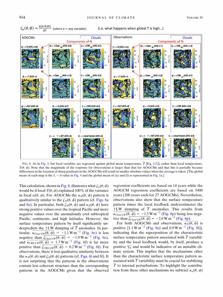
This calculation, shown in Fig. 8, illustrates what za(u,f)

would be if local T(u, f) explained 100% of the variance

in local a(u, f). For AOGCMs the kN(u, f) pattern is

qualitatively similar to the zN(u, f) pattern (cf. Figs. 6a

and 8a). In particular, both zN(u, f) and kN(u, f) have

strong positive values over the tropical Pacific and more

negative values over the anomalously cool subtropical

Pacific, continents, and high latitudes. However, the

surface temperature pattern by itself significantly un-

derpredicts the [LW damping of T anomalies. In par-

ticular, kClear LW(u, f) 5 21.1Wm22 (Fig. 8e) is less

negative than zClear LW(u, f) 5 21.9Wm22 (Fig. 6e),

and kCRELW(u, f) 5 1.7Wm22 (Fig. 8f) is far more

positive than zCRELW(u, f) 5 0.2Wm22 (Fig. 6f). For

observations, there is less qualitative similarity between

the kN(u, f) and zN(u, f) patterns (cf. Figs. 6l and 8l). It

is not surprising that the patterns in the observations

contain less coherent structure than the corresponding

patterns in the AOGCMs given that the observed

regression coefficients are based on 14 years while the

AOGCM regression coefficients are based on 5400

years (200 years each for 27 AOGCMs). Nevertheless,

observations also show that the surface temperature

pattern times the local feedback underestimates the

[LW damping of T anomalies. This results from

kClear LW(u, f) 5 21.5Wm22 (Fig. 8p) being less nega-

tive than zClear LW(u, f) 5 22.6Wm22 (Fig. 6p).

For both AOGCMs and observations, kN(u, f) is

positive [1.1Wm22 (Fig. 8a) and 0.9Wm22 (Fig. 8l)],

indicating that the superposition of the characteristic

surface temperature pattern associated with T variabil-

ity and the local feedback would, by itself, produce a

positive gN and would be indicative of an unstable cli-

mate system. This implies that the mechanisms other

than the characteristic surface temperature pattern as-

sociated with T variability must be crucial for stabilizing

T to internal perturbations. To highlight the contribu-

tion from these other mechanisms we subtract ka(u, f)

FIG. 6. As in Fig. 3, but local variables are regressed against global mean temperature, T [Eq. (12)], rather than local temperature,

T(u, f). Note that the magnitude of the response for observations is larger than that for AOGCMs and that this is partially because

differences in the location of sharp gradients in the AOGCMswill result in smaller absolute values when the average is taken. [The global

mean of each map is the L 5 0 value in Fig. 9 and the global mean of (a) and (l) is represented in Fig. 1a.]

934 JOURNAL OF CL IMATE VOLUME 29

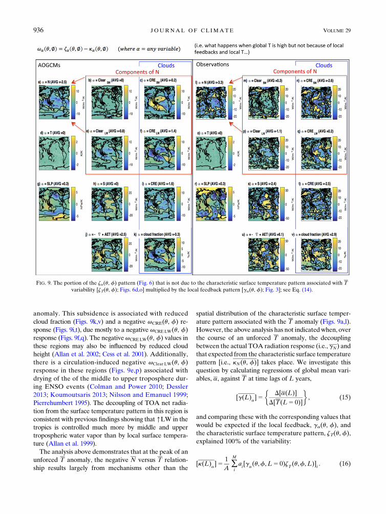
(Fig. 8) from the directly simulated or observed re-

lationship za(u, f) (Fig. 6),

va(u,f)5 z

a(u,f)2 k

a(u,f) , (14)

and plot these values in Fig. 9.

This calculation reveals that ka(u, f) greatly under-

predicts themagnitude of negativeN values overmuch of

the surface of the planet, particularly over the Pacific

tropics and subtropics (Figs. 9a,l). It is well known that

positive T (and thus positive ENSO) is associated with a

great amount of heat flux from the Pacific Ocean to the

atmosphere (Trenberth et al. 2002a; see Figs. 6h,s herein).

This anomalous heat flux causes a large reorganization of

the atmospheric circulation that leads to a strengthening

of the Hadley cell over the Pacific and alters the Walker

circulation leading to anomalous subsidence over In-

donesia (Klein et al. 1999). Figure 9 indicates that these

ENSO-specific atmospheric features are not heavily tied

to the characteristic T(u, f) pattern. In particular, the

patterns of zS(u, f) (Figs. 6h,s) and zSLP(u, f) (Figs. 6g,r)

are very similar to their corresponding patterns of

vS(u, f) (Figs. 9h,s) and vSLP(u, f) (Figs. 9g,r).

These ENSO-caused shifts in S and large-scale atmo-

spheric circulation have a profound impact on thevN(u,f)

pattern (Figs. 9a,l). In particular, the large negative

vN(u, f) values over Indonesia and the equatorial Atlantic

are associatedwith anomalously highvSLP(u,f) (Figs. 9g,r),

indicating that these are regions of anomalous subsidence

during positive T that are not caused by the local T(u, f)

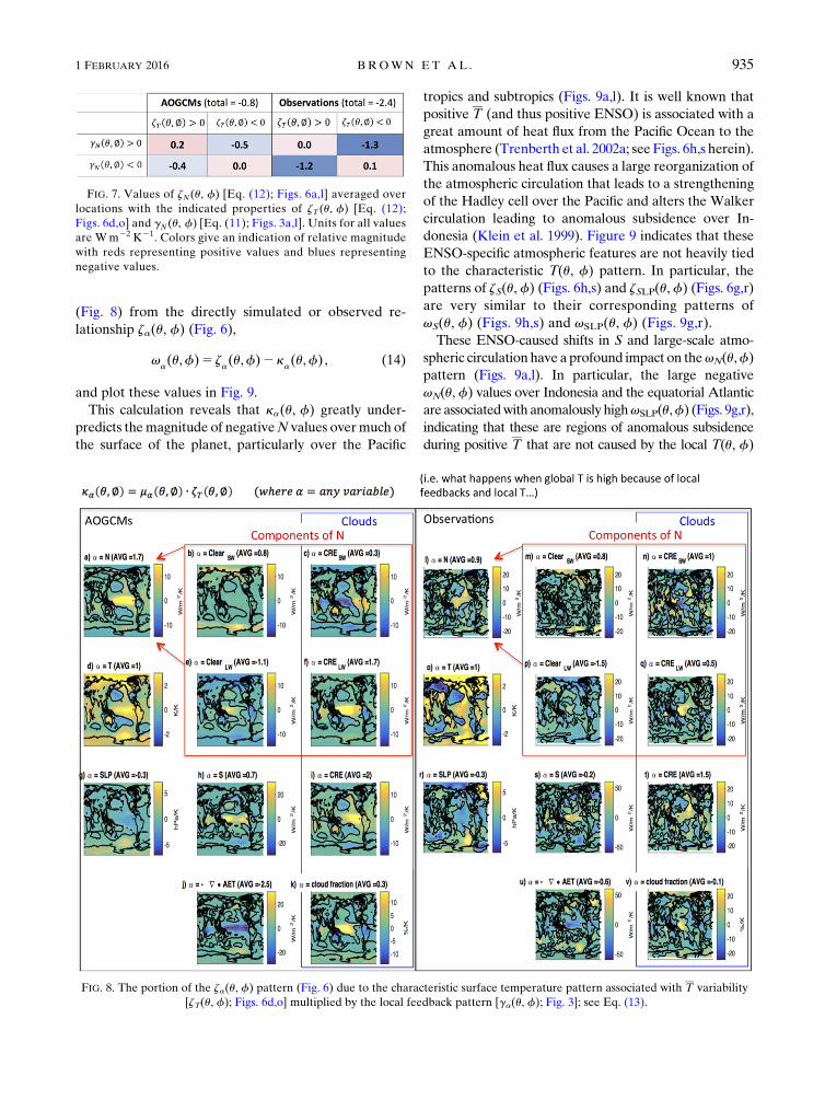
FIG. 7. Values of zN(u, f) [Eq. (12); Figs. 6a,l] averaged over

locations with the indicated properties of zT(u, f) [Eq. (12);

Figs. 6d,o] and gN(u, f) [Eq. (11); Figs. 3a,l]. Units for all values

are Wm22 K21. Colors give an indication of relative magnitude

with reds representing positive values and blues representing

negative values.

FIG. 8. The portion of the za(u, f) pattern (Fig. 6) due to the characteristic surface temperature pattern associated with T variability

[zT(u, f); Figs. 6d,o] multiplied by the local feedback pattern [ga(u, f); Fig. 3]; see Eq. (13).

1 FEBRUARY 2016 BROWN ET AL . 935

anomaly. This subsidence is associated with reduced

cloud fraction (Figs. 9k,v) and a negative vCRE(u, f) re-

sponse (Figs. 9i,t), due mostly to a negative vCRELW(u, f)

response (Figs. 9f,q). The negative vCRELW(u, f) values in

these regions may also be influenced by reduced cloud

height (Allan et al. 2002; Cess et al. 2001). Additionally,

there is a circulation-induced negative vClear LW(u, f)

response in these regions (Figs. 9e,p) associated with

drying of the of the middle to upper troposphere dur-

ing ENSO events (Colman and Power 2010; Dessler

2013; Koumoutsaris 2013; Nilsson and Emanuel 1999;

Pierrehumbert 1995). The decoupling of TOA net radia-

tion from the surface temperature pattern in this region is

consistent with previous findings showing that[LW in the

tropics is controlled much more by middle and upper

tropospheric water vapor than by local surface tempera-

ture (Allan et al. 1999).

The analysis above demonstrates that at the peak of an

unforced T anomaly, the negative N versus T relation-

ship results largely from mechanisms other than the

spatial distribution of the characteristic surface temper-

ature pattern associated with the T anomaly (Figs. 9a,l).

However, the above analysis has not indicatedwhen, over

the course of an unforced T anomaly, the decoupling

between the actual TOA radiation response (i.e., gN) and

that expected from the characteristic surface temperature

pattern [i.e., kN(u, f)] takes place. We investigate this

question by calculating regressions of global mean vari-

ables, a, against T at time lags of L years,

[g(L)a]5

�D[a(L)]

D[T(L5 0)]

�, (15)

and comparing these with the corresponding values that

would be expected if the local feedback, ga(u, f), and

the characteristic surface temperature pattern, zT(u, f),

explained 100% of the variability:

[k(L)a]5

1

A�M

i

ai[g

a(u,f,L5 0)z

T(u,f,L)]

i. (16)

FIG. 9. The portion of the za(u, f) pattern (Fig. 6) that is not due to the characteristic surface temperature pattern associated with T

variability [zT(u, f); Figs. 6d,o] multiplied by the local feedback pattern [ga(u, f); Fig. 3]; see Eq. (14).

936 JOURNAL OF CL IMATE VOLUME 29

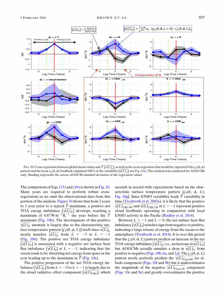
The comparison of Eqs. (15) and (16) is shown in Fig. 10.

Many years are required to perform robust cross-

regressions so we omit the observational data from this

portion of the analysis. Figure 10 shows that from 3 years

to 1 year prior to a typical T maximum, a positive net

TOA energy imbalance [g(L)N] develops, reaching a

maximum of 0.87Wm22K21 the year before the T

maximum (Fig. 10b). The development of this positive

g(L)N anomaly is largely due to the characteristic sur-

face temperature pattern [zT(u, f, L)] itself since k(L)Nnearly matches g(L)N from L 5 23 to L 5 21

(Fig. 10b). The positive net TOA energy imbalance

[g(L)N] is associated with a negative net surface heat

flux imbalance [g(L)S] at L 5 21, indicating that the

ocean tends to be absorbing net energy from space in the

year leading up to the maximum in T (Fig. 10c).

The positive progression of the net TOA energy im-

balance [g(L)N] fromL523 toL521 is largely due to

the cloud radiative effect component [g(L)CRE], which

ascends in accord with expectations based on the char-

acteristic surface temperature pattern [zT(u, f, L);

Fig. 10g]. Since ENSO variability leads T variability in

time (Trenberth et al. 2002a), it is likely that the positive

g(L)CRESW and g(L)CRELW atL521 represent positive

cloud feedbacks operating in conjunction with local

ENSO activity in the Pacific (Radley et al. 2014).

Between L 5 21 and L 5 0, the net surface heat flux

imbalance [g(L)S] switches sign fromnegative to positive,

indicating a large release of energy from the ocean to the

atmosphere (Trenberth et al. 2014). It is over this period

that the zT(u, f,L) pattern predicts an increase in the net

TOAenergy imbalance [g(L)N ; i.e., an increase ink(L)N]

but AOGCMs actually simulate a drop in g(L)N from

positive to negative (Figs. 10b, 6a, and 1a). The zT(u,f,L)

pattern nearly perfectly predicts the g(L)Clear SW ice al-

bedo component (Figs. 10f and 9b) but it underestimates

the magnitude of the negative g(L)ClearLW component

(Figs. 10e and 9e) and greatly overestimates the positive

FIG. 10. Cross regression between globalmean values andT [g(L)a], as well as the cross regression that would be expected if the zT(u,f)

pattern and the local ga(u, f) feedback explained 100% of the variability [k(L)a]; see Eq. (16). This analysis was conducted for AOGCMs

only. Shading represents the across-AOGCM standard deviation of the regression values.

1 FEBRUARY 2016 BROWN ET AL . 937

g(L)CRELW component. The implication is that during

the peak of a positive T anomaly (i.e., an El Niñoevent), there is a great amount of heat flux from the

ocean to the atmosphere where it can more easily be

emitted to space in the form of[LW.Additionally ENSO

dynamics cause a large-scale rearrangement of atmospheric

circulation that causes more efficient [LW (Figs. 10e,h)

due to drying and reduced cloud fraction over large por-

tions of Indo-Pacific tropics and subtropics. Overall, this

causes the net TOA energy imbalance [g(L)N] to reduce

to a negative value atL5 0 despite k(L)N continuing in its

positive ascent (Fig. 10b).

A year after the maximum in T, g(L)Clear SW remains

positive (Fig. 10f) but a negative g(L)Clear LW (Fig. 10e)

and a negative g(L)CRELW (Fig. 10h) help g(L)N remain

negative despite the tendency of the characteristic sur-

face temperature pattern [zT(u, f, L)] to induce a posi-

tive TOA net radiation imbalance [k(L)N ; Fig. 10b].

This negative TOA net radiation imbalance acts as a

restoring force, causing the T anomaly to return to its

equilibrium value.

6. Summary

In order for the unforced climate system to be stable

in the long run, it is expected that the global mean TOA

net radiation imbalance, N, will exhibit a negative

relationship with unforced global mean surface

temperature anomalies, T . We show that this nega-

tive relationship exists in both contemporary obser-

vations as well as in state-of-the-art AOGCMs.

However, we also show that, at the local spatial scale,

the simultaneous relationship between N(u, f) and

T(u, f) tends to be positive over most of the surface of

the planet. The reasons for the positive relationship

differ by geographic location and have a strong de-

pendence on the climatological mean T(u, f). The

locally positive relationship is mostly due to the

surface shortwave component (i.e., ice albedo feed-

back) for regions with T(u, f)clim values near the

freezing point of water, mostly due to the shortwave

cloud radiative effect component over regions with

intermediate to high T(u, f)clim values (from ;273 to

;300K), and mostly due to the longwave water vapor

feedback over oceanic regions with the highest

T(u, f)clim values.

The mostly positive N(u, f) versus T(u, f) relation-

ship at the local spatial scale can be reconciled with the

globally negative N versus T relationship when

anomalous atmospheric energy transport, the charac-

teristic surface temperature pattern, and adjustments

in the large-scale atmospheric circulation are consid-

ered. In particular, positive T anomalies are associated

with El Niño events in which there is large anomalous

heat flux from the Pacific Ocean into the atmosphere

where the local N(u, f) versus T(u, f) relationship is

positive. This leads to significant horizontal divergence

of atmospheric energy transport over the tropical Pa-

cific, and convergence of atmospheric energy transport

at high latitudes and specific continental regions. This

redistribution of energy helps create a characteristic

T(u, f) versus T pattern with a substantial amount of

warmth at high latitudes [characterized by a locally

negative N(u, f) versus T(u, f) relationship where the

temperature anomaly can be more easily damped to

space]. Additionally, the characteristic T(u, f) versus

T pattern contains anomalously coolT(u,f) regions where

a locally positive N(u, f) versus T(u, f) relationship

promotes a locally negative N(u, f).

However, the characteristic T(u, f) versus T pattern

by itself cannot explain the negative N versus T re-

lationship because a multiplication of the local N(u, f)

versus T(u, f) map by the T(u, f) versus T map

produces a positive estimate of the N versus T re-

lationship. This indicates that atmospheric circulation

changes associated with unforced interannual T vari-

ability are crucial in the explanation of the negative N

versus T relationship. In particular, a T maximum is

preceded, a year prior, by a positive N that is consistent

with expectations based on the T(u, f) versus T pattern.

However, simultaneous to the T peak, a great re-

arrangement of large-scale atmospheric circulation

causes reduced cloud cover and subsidence-induced

drying in broad regions of the tropical and subtropical

Indo-Pacific. This circulation change allows for much

more efficient release of [LW energy than would oth-

erwise be expected from the T(u, f) versus T pattern

alone. Because the short time scale relationship be-

tween N and T is heavily influenced by large-scale at-

mospheric circulation changes (opposed to local

feedbacks), this study supports the notion that there

may be very little relationship between the climate

feedback parameter (i.e., gN) diagnosed from annual or

subannual time scale variability and 2 3 CO2 equilib-

rium climate sensitivity.

Acknowledgments. We thank Dr. Drew Shindell for

helpful discussions on this topic. We acknowledge

Dr. Aaron Donohoe and two anonymous reviewers whose

comments greatly enhanced the manuscript. We ac-

knowledge the World Climate Research Programme’s

Working Group on Coupled Modelling, which is re-

sponsible for CMIP, and we thank the climate mod-

eling groups for producing and making available their

model output. For CMIP the U.S. Department of

Energy’s Program for Climate Model Diagnosis and

938 JOURNAL OF CL IMATE VOLUME 29

Intercomparison provides coordinating support and led

development of software infrastructure in partnership

with the Global Organization for Earth System Science

Portals. This work was partially supported by NSF

Grant AGS-1147608. We also acknowledge the support

from NASA ROSES13-NDOA, ROSES12-MAP, and

ROSES-NEWS programs. This research was partially

conducted at the Jet Propulsion Laboratory, California

Institute of Technology, sponsored by NASA.

REFERENCES

Alexander, M. A., I. Bladé, M. Newman, J. R. Lanzante, N.-C.

Lau, and J. D. Scott, 2002: The atmospheric bridge: The in-

fluence of ENSO teleconnections on air–sea interaction over

the global oceans. J. Climate, 15, 2205–2231, doi:10.1175/

1520-0442(2002)015,2205:TABTIO.2.0.CO;2.

Allan, R. P., K. P. Shine, A. Slingo, and J. A. Pamment, 1999:

The dependence of clear-sky outgoing long-wave ra-

diation on surface temperature and relative humidity.

Quart. J. Roy. Meteor. Soc., 125, 2103–2126, doi:10.1002/

qj.49712555809.

——, A. Slingo, and M. A. Ringer, 2002: Influence of dynamics

on the changes in tropical cloud radiative forcing during

the 1999 El Niño. J. Climate, 15, 1979–1986, doi:10.1175/

1520-0442(2002)015,1979:IODOTC.2.0.CO;2.

——, C. Liu, N. G. Loeb, M. D. Palmer, M. Roberts, D. Smith, and

P.-L. Vidale, 2014: Changes in global net radiative imbalance

1985–2012. Geophys. Res. Lett., 41, 5588–5597, doi:10.1002/

2014GL060962.

Armour, K. C., C. M. Bitz, and G. H. Roe, 2013: Time-varying

climate sensitivity from regional feedbacks. J. Climate, 26,

4518–4534, doi:10.1175/JCLI-D-12-00544.1.

Bellenger, H., E. Guilyardi, J. Leloup, M. Lengaigne, and

J. Vialard, 2014: ENSO representation in climate models:

From CMIP3 to CMIP5. Climate Dyn., 42, 1999–2018,

doi:10.1007/s00382-013-1783-z.

Bellomo, K., A. C. Clement, T. Mauritsen, G. Rädel, and

B. Stevens, 2014: Simulating the role of subtropical stratocu-

mulus clouds in driving Pacific climate variability. J. Climate,

27, 5119–5131, doi:10.1175/JCLI-D-13-00548.1.

——, ——, ——, ——, and ——, 2015: The influence of cloud

feedbacks on equatorial Atlantic variability. J. Climate, 28,

2725–2744, doi:10.1175/JCLI-D-14-00495.1.

Bony, S., and Coauthors, 2006: How well do we understand and

evaluate climate change feedback processes? J. Climate, 19,

3445–3482, doi:10.1175/JCLI3819.1.

Brown, P. T., W. Li, L. Li, and Y. Ming, 2014a: Top-of-atmosphere

radiative contribution to unforced decadal global temperature

variability in climate models. Geophys. Res. Lett., 41, 5175–

5183, doi:10.1002/2014GL060625.

——, ——, and S.-P. Xie, 2014b: Regions of significant influence

on unforced global mean surface air temperature variability

in climate models. J. Geophys. Res. Atmos., 120, 480–494,

doi:10.1002/2014JD022576.

——, ——, E. C. Cordero, and S. A. Mauget, 2015: Comparing the

model-simulated global warming signal to observations using

empirical estimates of unforced noise. Sci. Rep., 5, 9957,

doi:10.1038/srep09957.

Cess, R. D., M. Zhang, B. A. Wielicki, D. F. Young, X.-L.

Zhou, and Y. Nikitenko, 2001: The influence of the 1998

El Niño upon cloud-radiative forcing over the Pacific

warm pool. J. Climate, 14, 2129–2137, doi:10.1175/

1520-0442(2001)014,2129:TIOTEN.2.0.CO;2.

Chen, X., and K.-K. Tung, 2014: Varying planetary heat sink led

to global-warming slowdown and acceleration. Science, 345,

897–903, doi:10.1126/science.1254937.

Colman, R., and S. Power, 2010: Atmospheric radiative feed-

backs associated with transient climate change and cli-

mate variability. Climate Dyn., 34, 919–933, doi:10.1007/

s00382-009-0541-8.

Crook, J. A., P. M. Forster, and N. Stuber, 2011: Spatial patterns of

modeled climate feedback and contributions to temperature

response and polar amplification. J. Climate, 24, 3575–3592,

doi:10.1175/2011JCLI3863.1.

Dee, D. P., and Coauthors, 2011: The ERA-Interim reanalysis:

Configuration and performance of the data assimilation system.

Quart. J. Roy. Meteor. Soc., 137, 553–597, doi:10.1002/qj.828.Deser, C., M. A. Alexander, S.-P. Xie, and A. S. Phillips, 2010:

Sea surface temperature variability: Patterns and mecha-

nisms. Annu. Rev. Mar. Sci., 2, 115–143, doi:10.1146/

annurev-marine-120408-151453.

Dessler, A. E., 2010: A determination of the cloud feedback from

climate variations over the past decade. Science, 330, 1523–

1527, doi:10.1126/science.1192546.

——, 2013: Observations of climate feedbacks over 2000–10 and

comparisons to climate models. J. Climate, 26, 333–342,

doi:10.1175/JCLI-D-11-00640.1.

Dolinar, E., X. Dong, B. Xi, J. Jiang, andH. Su, 2015: Evaluation of

CMIP5 simulated clouds and TOA radiation budgets using

NASA satellite observations. Climate Dyn., 44, 2229–2247,

doi:10.1007/s00382-014-2158-9.

Donohoe, A., and D. S. Battisti, 2011: Atmospheric and surface

contributions to planetary albedo. J. Climate, 24, 4402–4418,

doi:10.1175/2011JCLI3946.1.

Drijfhout, S. S., A. T. Blaker, S. A. Josey, A. J. G. Nurser, B. Sinha,

andM.A. Balmaseda, 2014: Surface warming hiatus caused by

increased heat uptake across multiple ocean basins.Geophys.

Res. Lett., 41, 7868–7874, doi:10.1002/2014GL061456.

Emery, W. J., and K. Hamilton, 1985: Atmospheric forcing of in-

terannual variability in the northeast Pacific Ocean: Connec-

tions with El Niño. J. Geophys. Res., 90, 857–868, doi:10.1029/

JC090iC01p00857.

England, M. H., and Coauthors, 2014: Recent intensification of

wind-driven circulation in the Pacific and the ongoing warm-

ing hiatus. Nat. Climate Change, 4, 222–227, doi:10.1038/

nclimate2106.

Evan, A. T., R. J. Allen, R. Bennartz, and D. J. Vimont, 2013: The

modification of sea surface temperature anomaly linear

damping time scales by stratocumulus clouds. J. Climate, 26,

3619–3630, doi:10.1175/JCLI-D-12-00370.1.

Folland, C. K., J. A. Renwick, M. J. Salinger, and A. B. Mullan,

2002: Relative influences of the interdecadal Pacific oscillation

and ENSO on the South Pacific convergence zone. Geophys.

Res. Lett., 29, 1643, doi:10.1029/2001GL014201.

Hallberg, R., and A. K. Inamdar, 1993: Observations of seasonal

variations in atmospheric greenhouse trapping and its enhance-

ment at high sea surface temperature. J. Climate, 6, 920–931,

doi:10.1175/1520-0442(1993)006,0920:OOSVIA.2.0.CO;2.

Hasselmann, K., 1976: Stochastic climate models. Part I: Theory.

Tellus, 28A, 473–485, doi:10.1111/j.2153-3490.1976.tb00696.x.

Hawkins, E., and R. Sutton, 2009: The potential to narrow un-

certainty in regional climate predictions. Bull. Amer. Meteor.

Soc., 90, 1095–1107, doi:10.1175/2009BAMS2607.1.

1 FEBRUARY 2016 BROWN ET AL . 939

Inamdar, A. K., and V. Ramanathan, 1994: Physics of greenhouse

effect and convection in warm oceans. J. Climate, 7, 715–731,

doi:10.1175/1520-0442(1994)007,0715:POGEAC.2.0.CO;2.

Ingram, W., 2013: Some implications of a new approach to the

water vapour feedback. Climate Dyn., 40, 925–933, doi:10.1007/

s00382-012-1456-3.

Kato, S., 2009: Interannual variability of the global radiation budget.

J. Climate, 22, 4893–4907, doi:10.1175/2009JCLI2795.1.Kiehl, J. T., 1994: On the observed near cancellation between

longwave and shortwave cloud forcing in tropical regions.

J. Climate, 7, 559–565, doi:10.1175/1520-0442(1994)007,0559:

OTONCB.2.0.CO;2.

Klein, S. A., B. J. Soden, and N.-C. Lau, 1999: Remote sea surface

temperature variations during ENSO: Evidence for a tropi-

cal atmospheric bridge. J. Climate, 12, 917–932, doi:10.1175/1520-0442(1999)012,0917:RSSTVD.2.0.CO;2.

Kosaka, Y., and S.-P. Xie, 2013: Recent global-warming hiatus tied

to equatorial Pacific surface cooling. Nature, 501, 403–407,

doi:10.1038/nature12534.

Koumoutsaris, S., 2013: What can we learn about climate feed-

backs from short-term climate variations? Tellus, 65A, 18887,

doi:10.3402/tellusa.v65i0.18887.

Larson, K., and D. L. Hartmann, 2003: Interactions among cloud,

water vapor, radiation, and large-scale circulation in the

tropical climate. Part I: Sensitivity to uniform sea surface

temperature changes. J. Climate, 16, 1425–1440, doi:10.1175/1520-0442-16.10.1425.

Lau, N.-C., andM. J. Nath, 1994: A modeling study of the relative

roles of tropical and extratropical SST anomalies in the

variability of the global atmosphere–ocean system. J. Cli-

mate, 7, 1184–1207, doi:10.1175/1520-0442(1994)007,1184:

AMSOTR.2.0.CO;2.

Loeb, N., and Coauthors, 2012: Advances in understanding top-of-

atmosphere radiation variability from satellite observations.

Surv. Geophys., 33, 359–385, doi:10.1007/s10712-012-9175-1.

Meehl, G. A., A. Hu, J. M. Arblaster, J. Fasullo, and K. E.

Trenberth, 2013: Externally forced and internally generated

decadal climate variability associated with the interdecadal

Pacific oscillation. J. Climate, 26, 7298–7310, doi:10.1175/

JCLI-D-12-00548.1.

Minnis, P., and Coauthors, 2011: CERES edition-2 cloud property

retrievals using TRMM VIRS and Terra and Aqua MODIS

data—Part I: Algorithms. IEEE Trans. Geosci. Remote Sens.,

49, 4374–4400.

Nilsson, J., andK.A. Emanuel, 1999: Equilibrium atmospheres of a

two-column radiative-convective model. Quart. J. Roy. Me-

teor. Soc., 125, 2239–2264, doi:10.1002/qj.49712555814.

Palmer, M. D., and D. J. McNeall, 2014: Internal variability of

Earth’s energy budget simulated by CMIP5 climate models.

Environ. Res. Lett., 9, 034016, doi:10.1088/1748-9326/9/3/

034016.

Park, S., C. Deser, and M. A. Alexander, 2005: Estimation of the

surface heat flux response to sea surface temperature anom-

alies over the global oceans. J. Climate, 18, 4582–4599,

doi:10.1175/JCLI3521.1.

Pierrehumbert, R. T., 1995: Thermostats, radiator fins, and the

local runaway greenhouse. J. Atmos. Sci., 52, 1784–1806,

doi:10.1175/1520-0469(1995)052,1784:TRFATL.2.0.CO;2.

Radley, C., S. Fueglistaler, and L. Donner, 2014: Cloud and radiative

balance changes in response toENSOinobservations andmodels.

J. Climate, 27, 3100–3113, doi:10.1175/JCLI-D-13-00338.1.

Ramanathan, V., andW. Collins, 1991: Thermodynamic regulation

of ocean warming by cirrus clouds deduced from observations

of the 1987 El Niño.Nature, 351, 27–32, doi:10.1038/351027a0.

——, R. D. Cess, E. F. Harrison, P. Minnis, B. R. Barkstrom,

E. Ahmad, and D. Hartmann, 1989: Cloud-radiative forcing

and climate: Results from the Earth Radiation Budget Exper-

iment. Science, 243, 57–63, doi:10.1126/science.243.4887.57.

Smith, D. M., and Coauthors, 2015: Earth’s energy imbalance since

1960 in observations and CMIP5 models.Geophys. Res. Lett.,

42, 1205–1213, doi:10.1002/2014GL062669.

Soden,B. J.,A. J.Broccoli, andR. S.Hemler, 2004:On theuseof cloud

forcing to estimate cloud feedback. J. Climate, 17, 3661–3665,doi:10.1175/1520-0442(2004)017,3661:OTUOCF.2.0.CO;2.

Su, H., W. G. Read, J. H. Jiang, J. W. Waters, D. L. Wu, and E. J.

Fetzer, 2006: Enhanced positive water vapor feedback asso-

ciated with tropical deep convection: New evidence from

Aura MLS. Geophys. Res. Lett., 33, L05709, doi:10.1029/

2005GL025505.

Taylor, K. E., R. J. Stouffer, andG.A.Meehl, 2012:An overview of

CMIP5 and the experiment design. Bull. Amer. Meteor. Soc.,

93, 485–498, doi:10.1175/BAMS-D-11-00094.1.

Trenberth, K. E., and D. J. Shea, 2005: Relationships between

precipitation and surface temperature.Geophys. Res. Lett., 32,L14703, doi:10.1029/2005GL022760.

——, G. W. Branstator, D. Karoly, A. Kumar, N.-C. Lau, and

C.Ropelewski, 1998: Progress during TOGA in understanding

and modeling global teleconnections associated with tropical

sea surface temperatures. J. Geophys. Res., 103, 14 291–14 324,

doi:10.1029/97JC01444.

——, J.M. Caron,D. P. Stepaniak, and S.Worley, 2002a: Evolution

of El Niño–Southern Oscillation and global atmospheric sur-

face temperatures. J. Geophys. Res., 107, 4065, doi:10.1029/

2000JD000298.

——, D. P. Stepaniak, and J. M. Caron, 2002b: Interannual varia-

tions in the atmospheric heat budget. J. Geophys. Res., 107,

4066, doi:10.1029/2000JD000297.

——, J. T. Fasullo, C. O’Dell, and T. Wong, 2010: Relationships

between tropical sea surface temperature and top-of-atmosphere

radiation. Geophys. Res. Lett., 37, L03702, doi:10.1029/

2009GL042314.

——, ——, and M. A. Balmaseda, 2014: Earth’s energy imbalance.

J. Climate, 27, 3129–3144, doi:10.1175/JCLI-D-13-00294.1.

——,Y.Zhang, J. T. Fasullo, andS. Taguchi, 2015:Climate variability

and relationships between top-of-atmosphere radiation and

temperatures onEarth. J.Geophys. Res. Atmos., 120, 3642–3659,doi:10.1002/2014JD022887.

Trzaska, S., A. W. Robertson, J. D. Farrara, and C. R. Mechoso,

2007: South Atlantic variability arising from air–sea coupling:

Local mechanisms and tropical–subtropical interactions.

J. Climate, 20, 3345–3365, doi:10.1175/JCLI4114.1.

Webb,M. J., andA.Lock, 2013: Coupling between subtropical cloud

feedback and the local hydrological cycle in a climate model.

Climate Dyn., 41, 1923–1939, doi:10.1007/s00382-012-1608-5.

Wielicki, B. A., B. R. Barkstrom, E. F. Harrison, R. B. Lee,

G. Louis Smith, and J. E. Cooper, 1996: Clouds and theEarth’s

Radiant Energy System (CERES): An Earth observing

system experiment. Bull. Amer. Meteor. Soc., 77, 853–868,

doi:10.1175/1520-0477(1996)077,0853:CATERE.2.0.CO;2.

Wigley, T. M. L., 2000: ENSO, volcanoes and record-breaking

temperatures.Geophys. Res. Lett., 27, 4101–4104, doi:10.1029/2000GL012159.

940 JOURNAL OF CL IMATE VOLUME 29