EMULATING GCM PROJECTIONS BY PATTERN SCALING •

PERFORMANCE •

UNFORCED CLIMATE VARIABILITY

Liege, September 2015

Tim Osborn, Craig Wallace Climatic Research Unit, School of Environmental Sciences, UEA, UK

• With contributions from Jason Lowe, Dan Bernie

Meteorological Office Hadley Centre, UK

WHAT IS PATTERN SCALING?

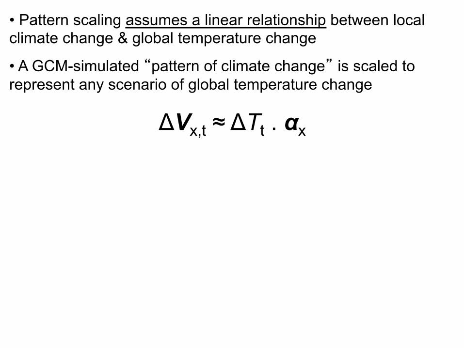
•  Pattern scaling assumes a linear relationship between local climate change & global temperature change

•  A GCM-simulated “pattern of climate change” is scaled to represent any scenario of global temperature change

ΔVx,t ≈ ΔTt . αx

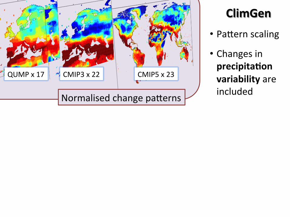
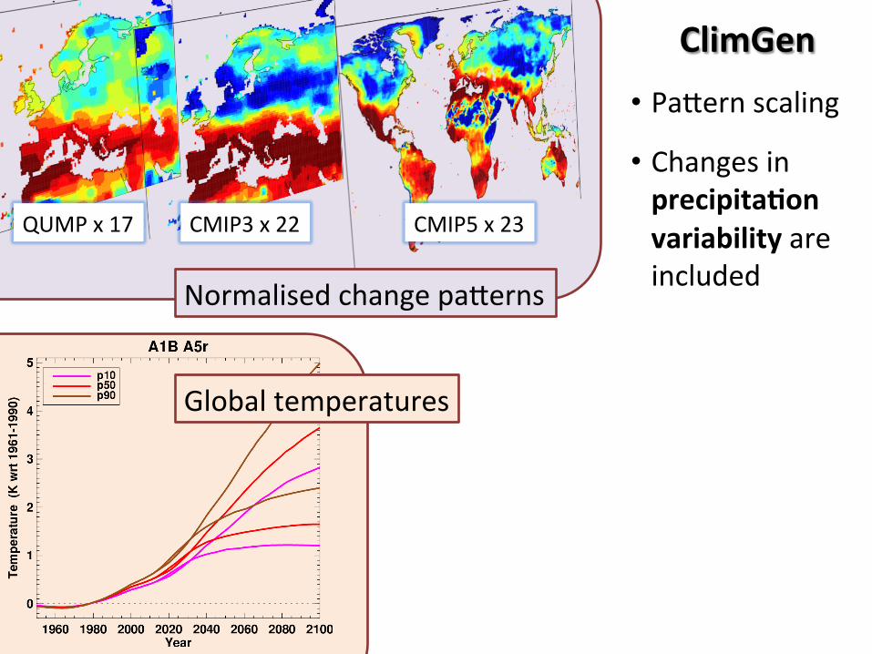
CMIP3  x  22   CMIP5  x  23  QUMP  x  17  

Normalised  change  pa=erns  

ClimGen  •  Pa=ern  scaling  

•  Changes  in  precipita.on  variability  are  included  

CMIP3  x  22   CMIP5  x  23  QUMP  x  17  

Global  temperatures  

Normalised  change  pa=erns  

ClimGen  •  Pa=ern  scaling  

•  Changes  in  precipita.on  variability  are  included  

CMIP3  x  22   CMIP5  x  23  QUMP  x  17  

Pa=ern  scaling  Global  temperatures  

Normalised  change  pa=erns  

ClimGen  •  Pa=ern  scaling  

•  Changes  in  precipita.on  variability  are  included  

CMIP3  x  22   CMIP5  x  23  QUMP  x  17  

Pa=ern  scaling  Global  temperatures  

Normalised  change  pa=erns  

ClimGen  •  Pa=ern  scaling  

•  Changes  in  precipita.on  variability  are  included  

•  Pattern scaling assumes a linear relationship between local climate change & global temperature change

•  A GCM-simulated “pattern of climate change” is scaled to represent any scenario of global temperature change

ΔVx,t ≈ ΔTt . αx •  If the linear assumption is correct, the pattern-scaled climate projection should match (emulate) what the GCM would have simulated for that scenario

•  But, is this assumption valid?

NO

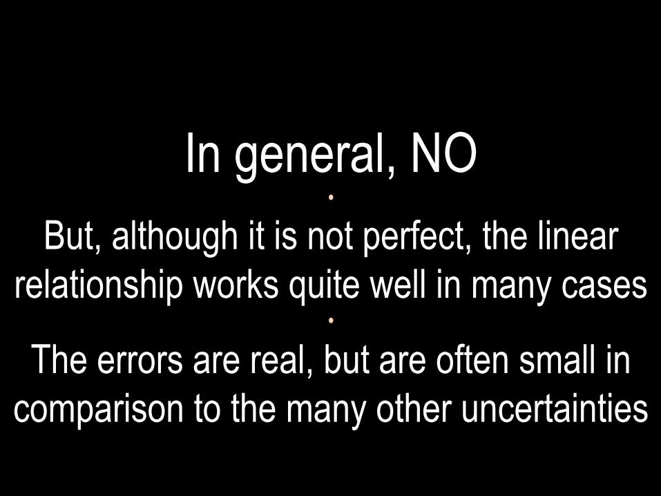
In general, NO •

But, although it is not perfect, the linear relationship works quite well in many cases

•

The errors are real, but are often small in comparison to the many other uncertainties

PATTERN SCALING PERFORMANCE

Climate timeseries (observed or GCM-simulated) are climate response to forcings plus a realisation of unforced (internally-generated) climate variability We’re interested in both but prefer to deal with them separately, not least because you cannot generate a sequence of unforced variability by pattern-scaling For ClimGen, we try to obtain patterns that represent the forced climate response: •  Use initial condition ensembles (where available) •  Pool simulations across multiple forcing scenarios (all RCPs) •  Regress change against global ΔT using all 1951-2100 data

Forced climate response & unforced climate variability

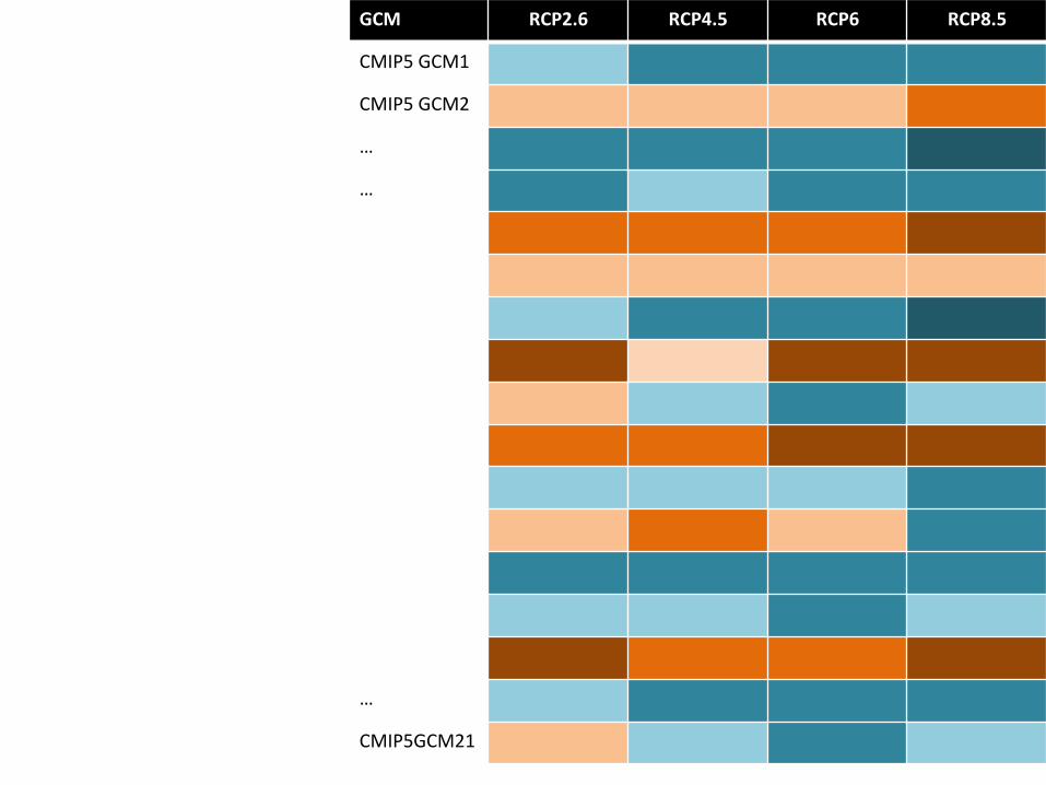
GCM   RCP2.6   RCP4.5   RCP6   RCP8.5  

CMIP5  GCM1  

CMIP5  GCM2  

…  

…  

…  

CMIP5GCM21  

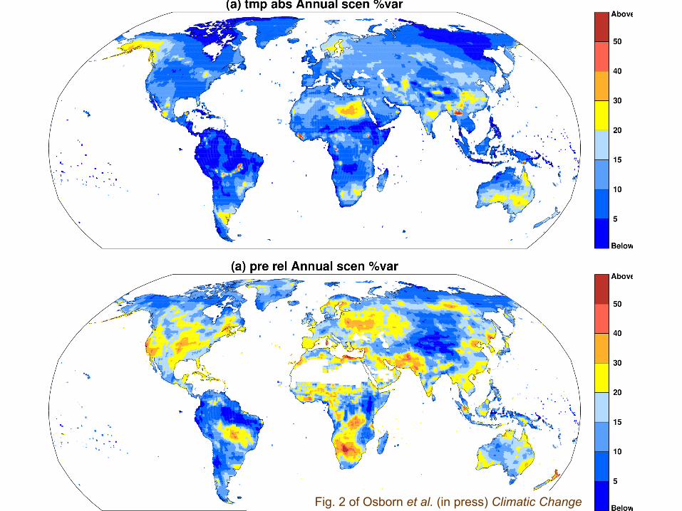
Fig. 2 of Osborn et al. (in press) Climatic Change

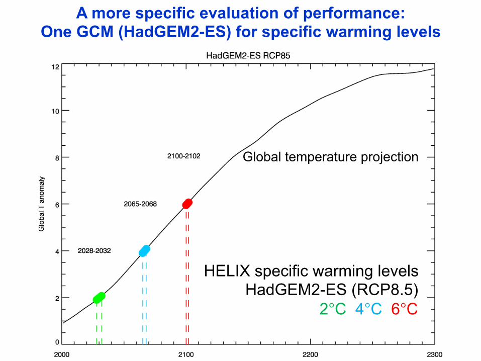
Global temperature projection

HELIX specific warming levels HadGEM2-ES (RCP8.5)

2°C 4°C 6°C

A more specific evaluation of performance: One GCM (HadGEM2-ES) for specific warming levels

PATTERN SCALING PERFORMANCE •

LAND AIR TEMPERATURE

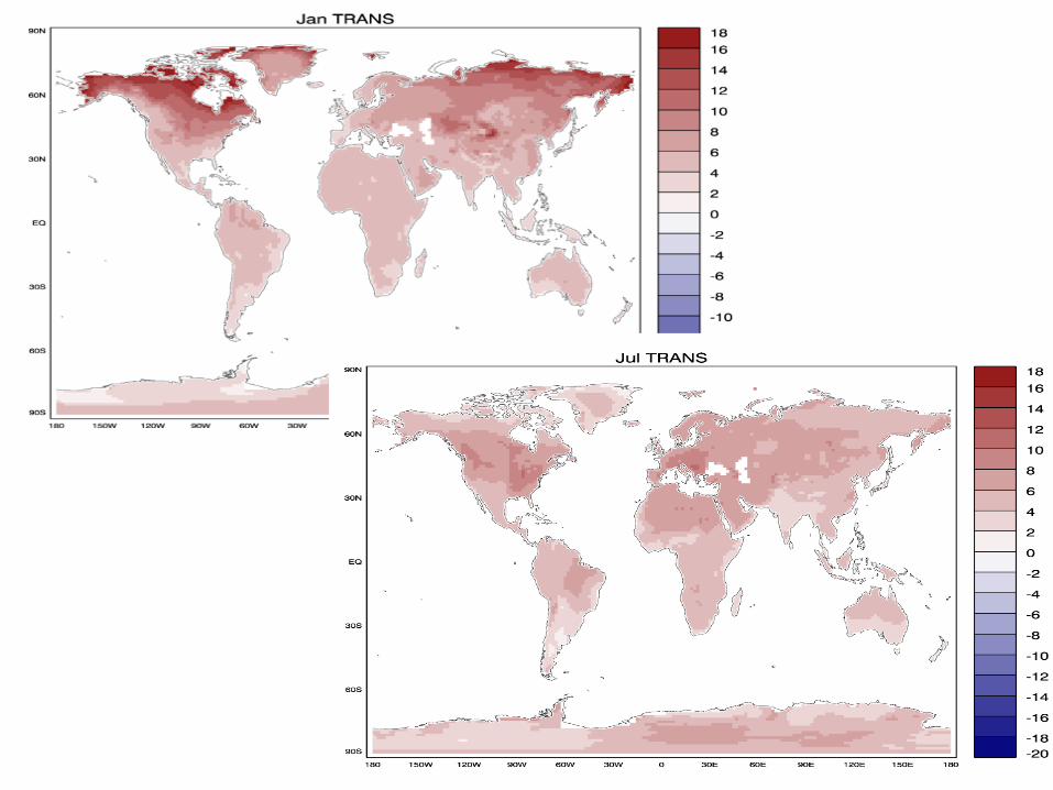
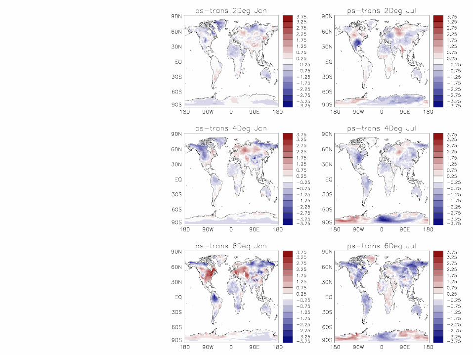
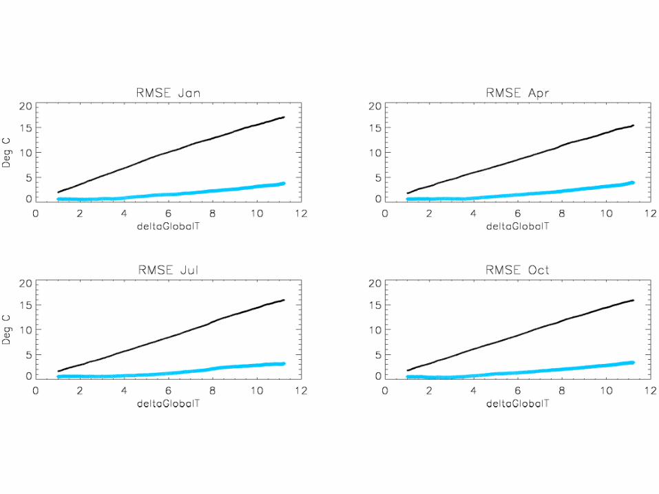
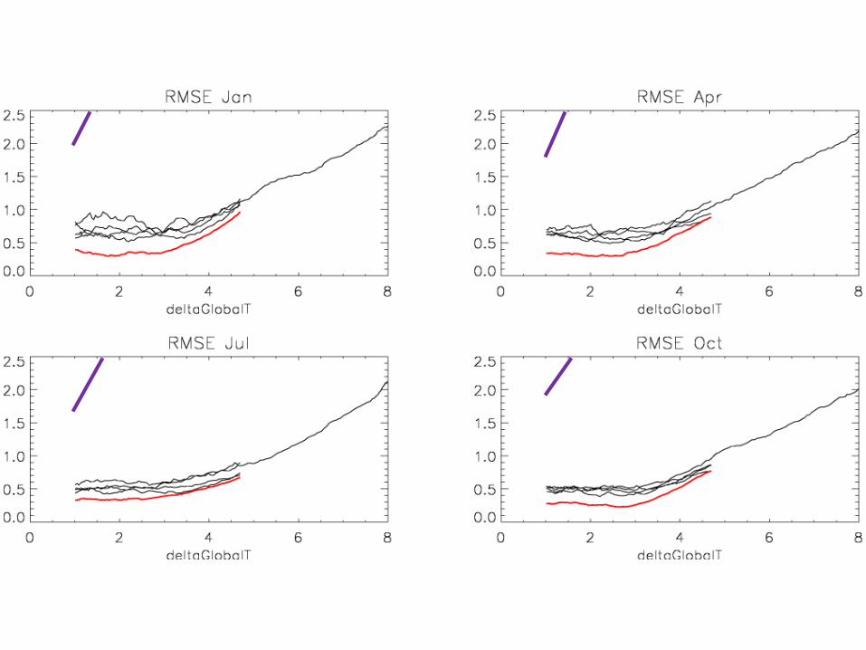
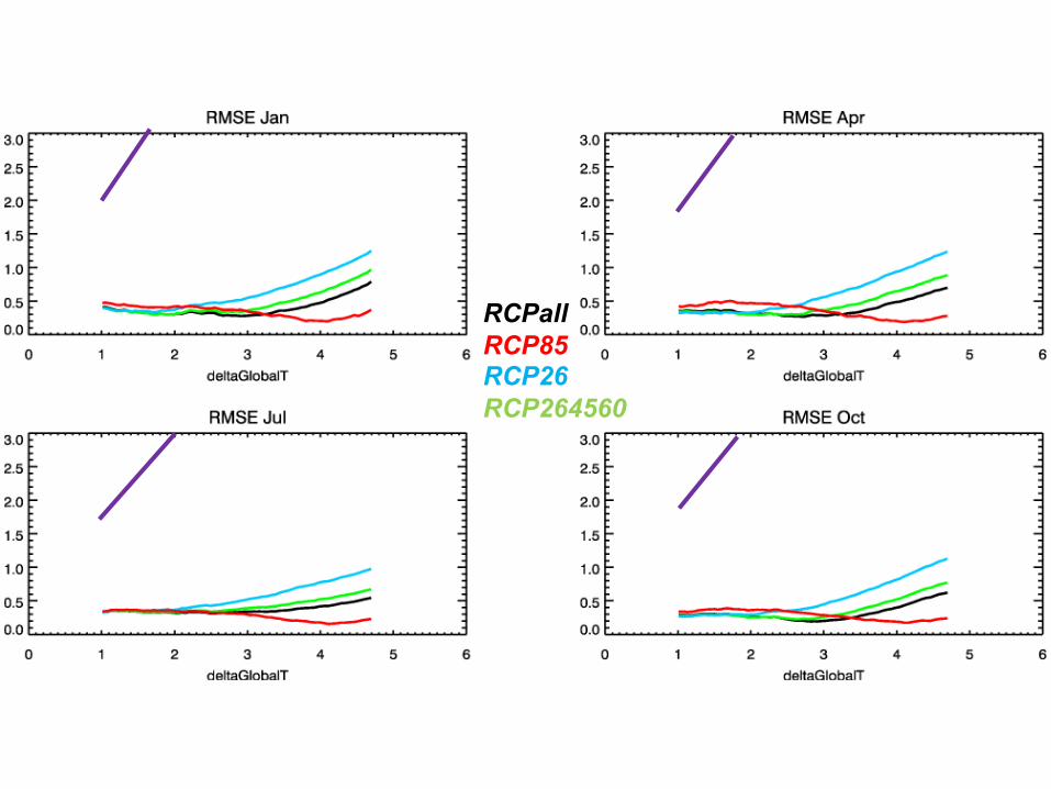
RCPall RCP85 RCP26 RCP264560

PATTERN SCALING PERFORMANCE •

LAND PRECIPITATION

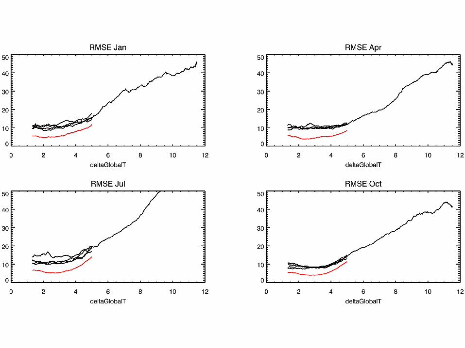
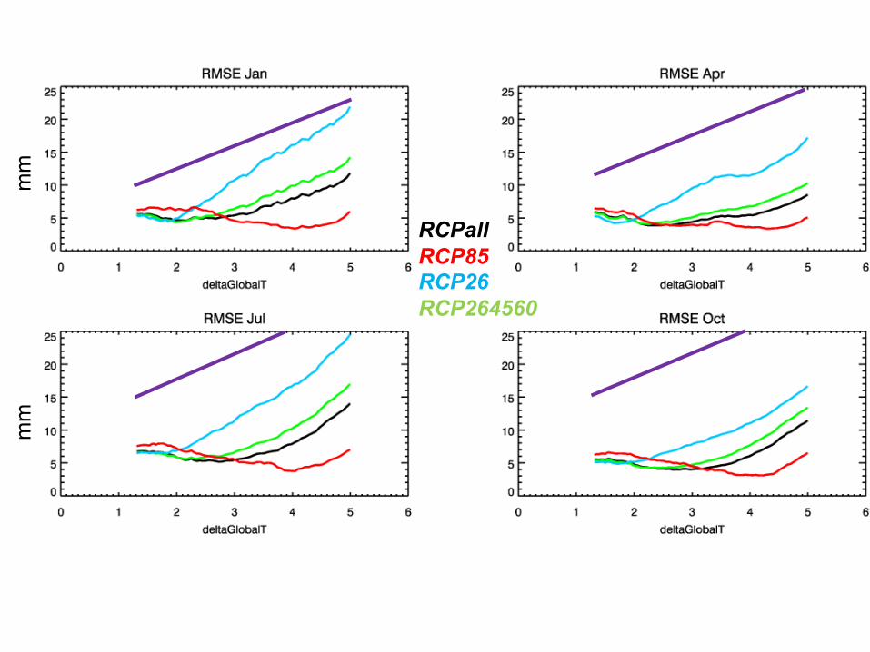
mm

m

m

RCPall RCP85 RCP26 RCP264560

FORCED CHANGES IN VARIABILITY •

PATTERN-SCALING METRICS OF VARIABILITY

Pattern scaling: unforced climate variability changes?

Pa=ern-­‐scale  higher  moments  (e.g.  standard  deviaGon,  skew)  •  We  divide  GCM  monthly  precipitaGon  Gmeseries  by  low-­‐pass  filter  •  Represent  the  high-­‐frequency  deviaGons  with  a  gamma  distribuGon  •  Scale  changes  in  gamma  shape  parameter  with  ΔT  

Fig. 1 of Osborn et al. (in press) Climatic Change

Rel

ativ

e ch

ange

in

How to utilise projected changes in distribution shape? Perturb the observations

Example  applicaGon  •  SE  England  grid  cell,  HadCM3  GCM,  July  precipitaGon  •  For  ΔT  =  3°C,  pa=ern-­‐scaling  gives  45%  reducGon  in  mean  precipitaGon  •  But  also  62%  reducGon  in  gamma  shape  param.  of  monthly  precipitaGon  

Fig. 1 of Osborn et al. (in press) Climatic Change

Observed sequence

Sequence x 0.55 Sequence x 0.55

Sequence x 0.55 & perturbed to have 62% lower shape

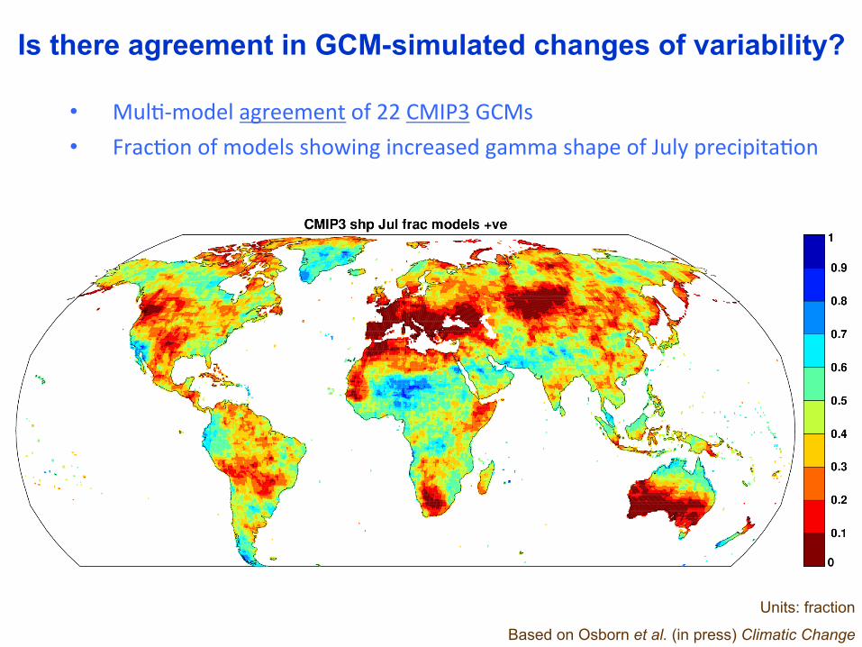
Is there agreement in GCM-simulated changes of variability?

•  MulG-­‐model  agreement  of  22  CMIP3  GCMs  •  FracGon  of  models  showing  increased  gamma  shape  of  July  precipitaGon  

Units: fraction

Based on Osborn et al. (in press) Climatic Change

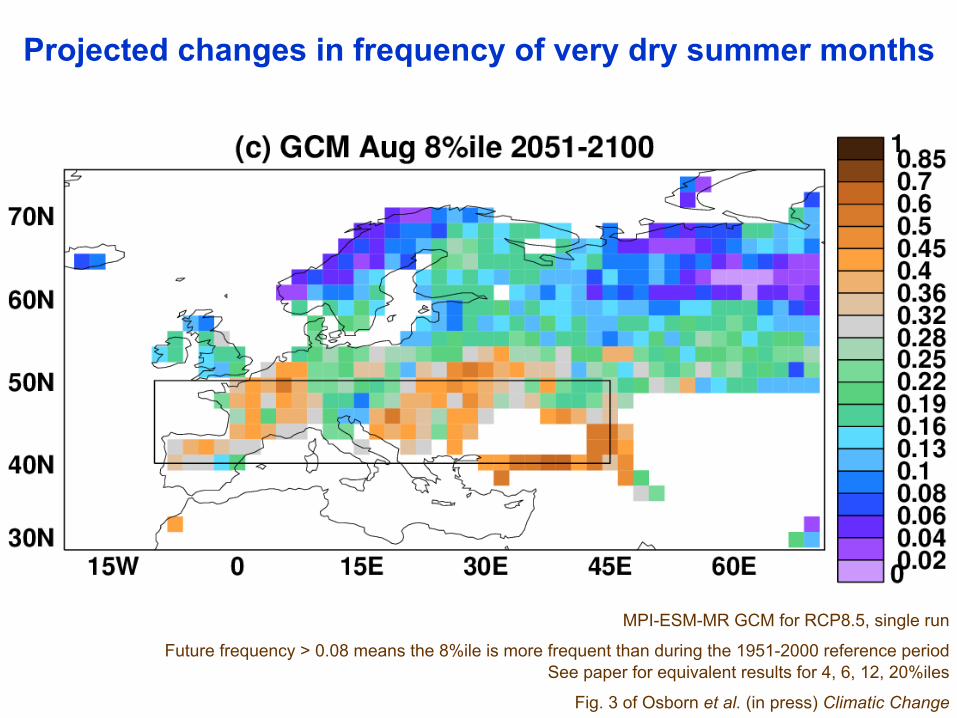
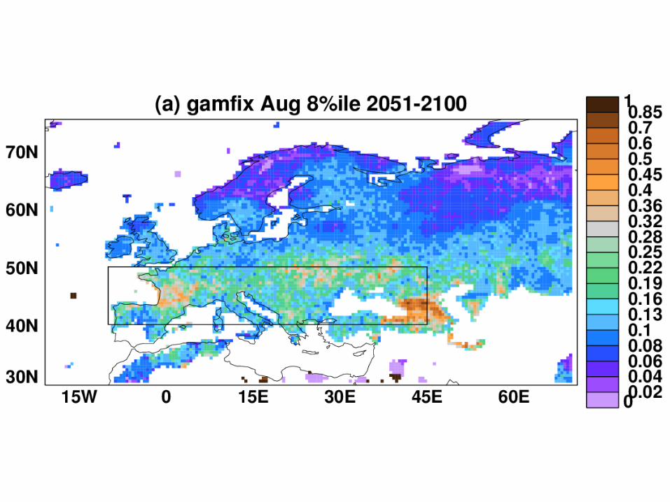
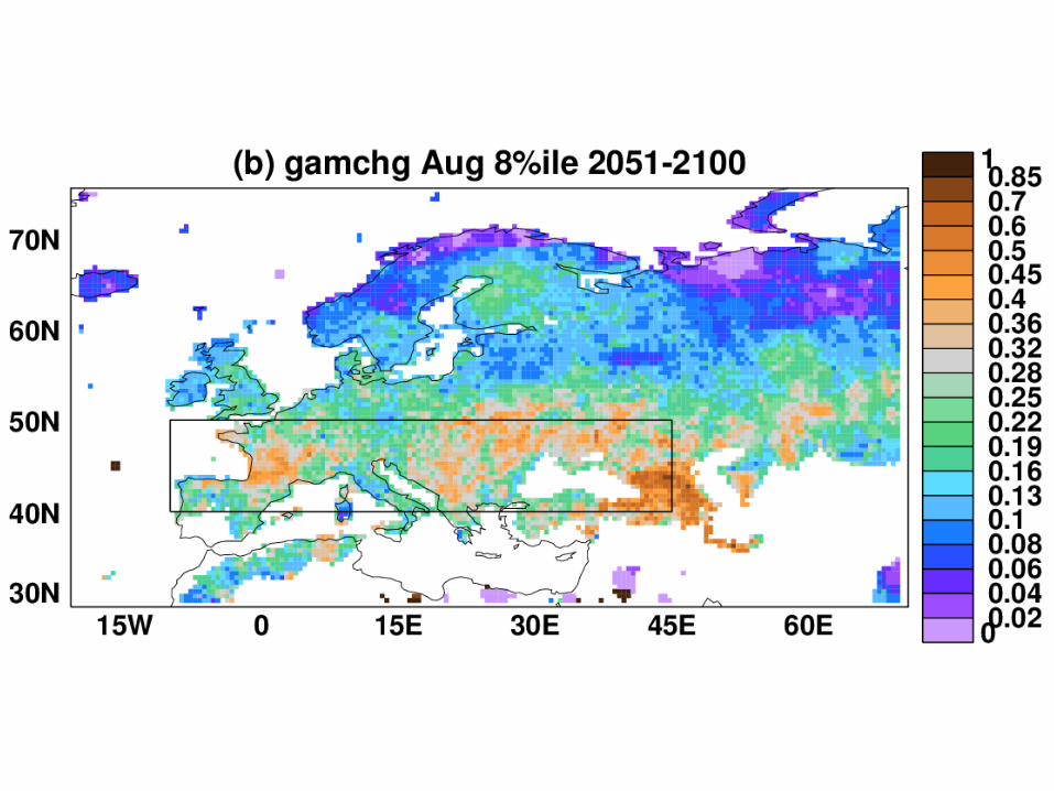
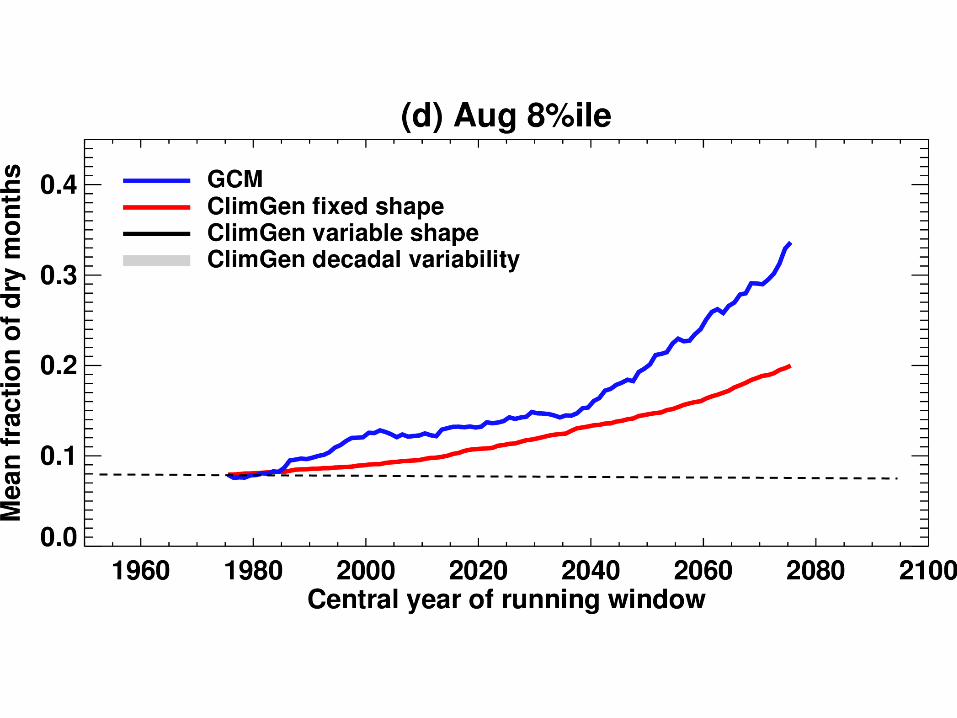
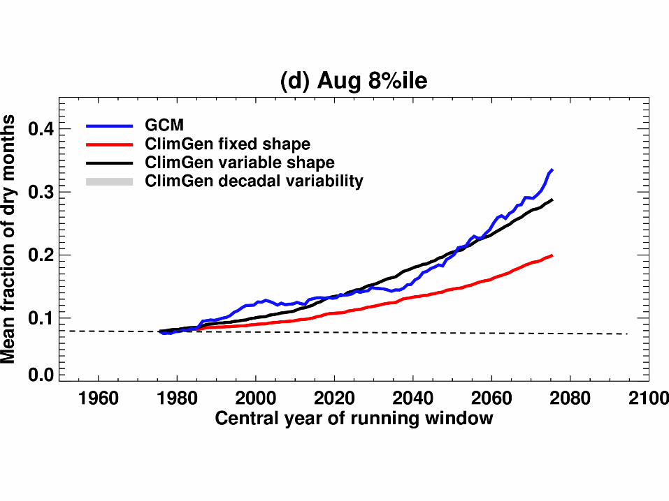
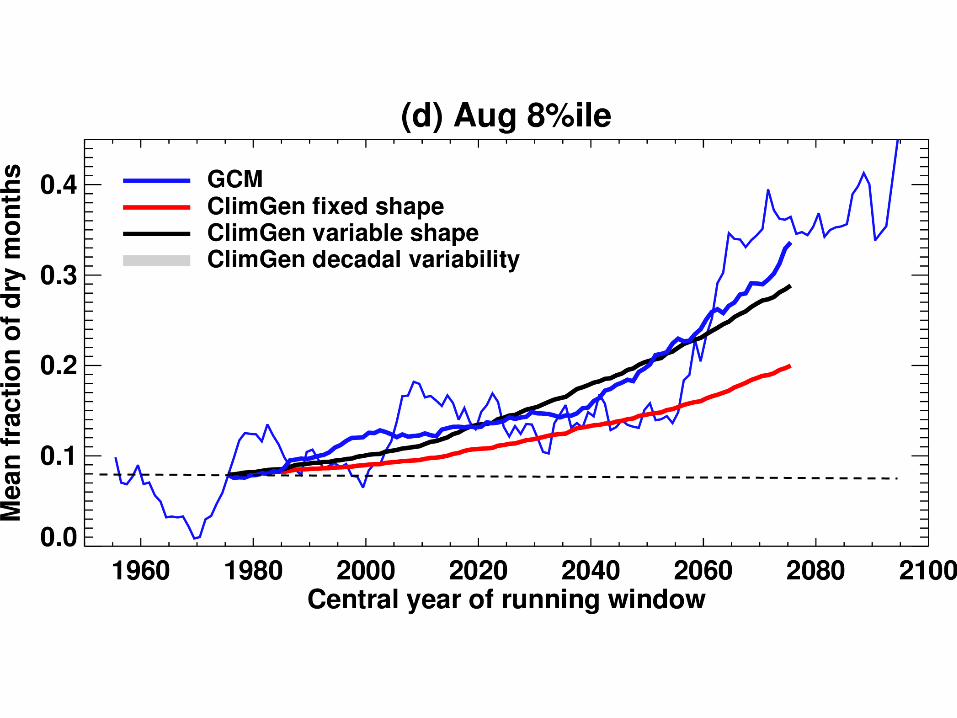
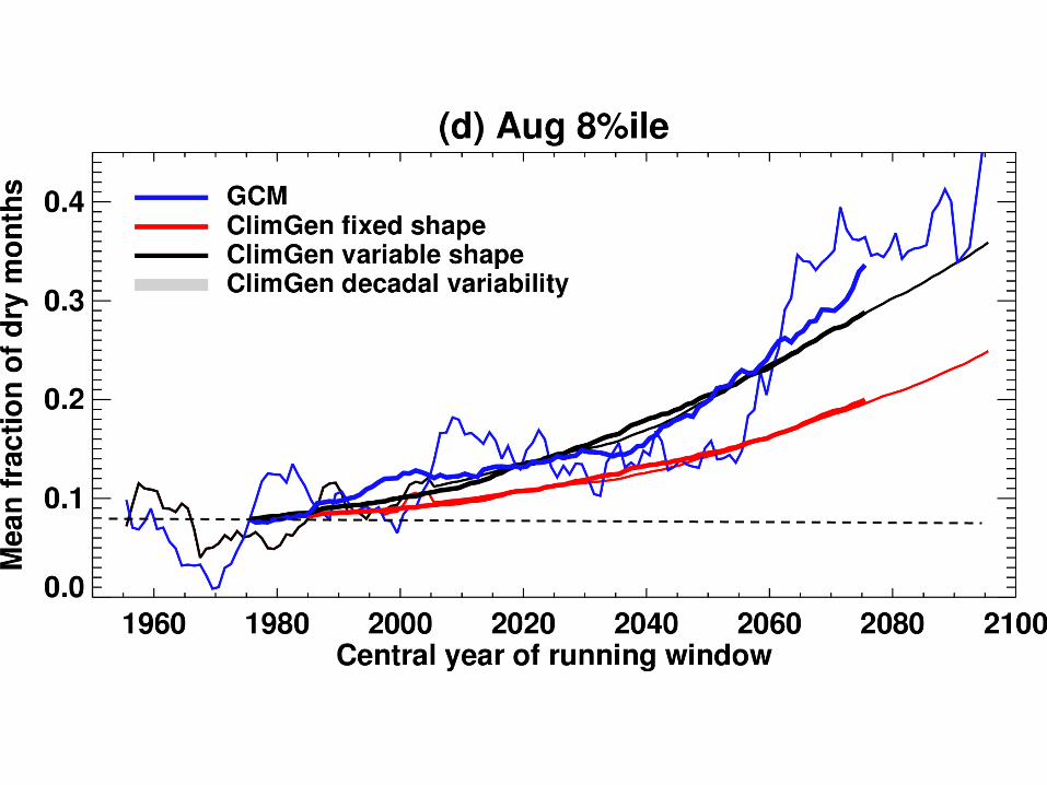
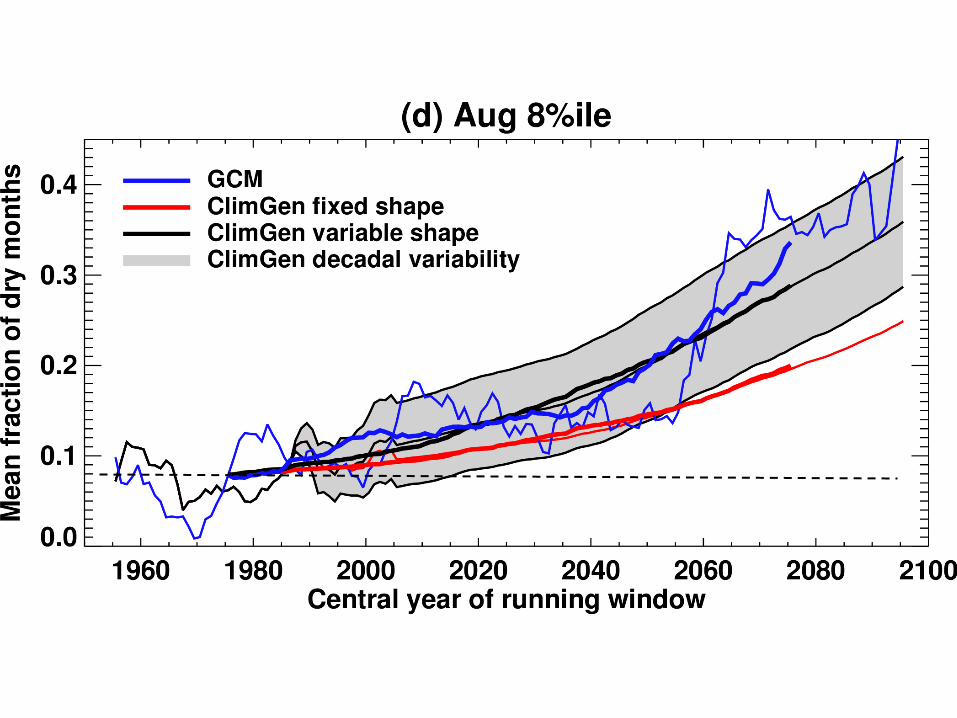
MPI-ESM-MR GCM for RCP8.5, single run

Future frequency > 0.08 means the 8%ile is more frequent than during the 1951-2000 reference period See paper for equivalent results for 4, 6, 12, 20%iles

Fig. 3 of Osborn et al. (in press) Climatic Change

Projected changes in frequency of very dry summer months

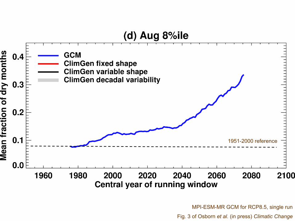
MPI-ESM-MR GCM for RCP8.5, single run

Fig. 3 of Osborn et al. (in press) Climatic Change

1951-2000 reference

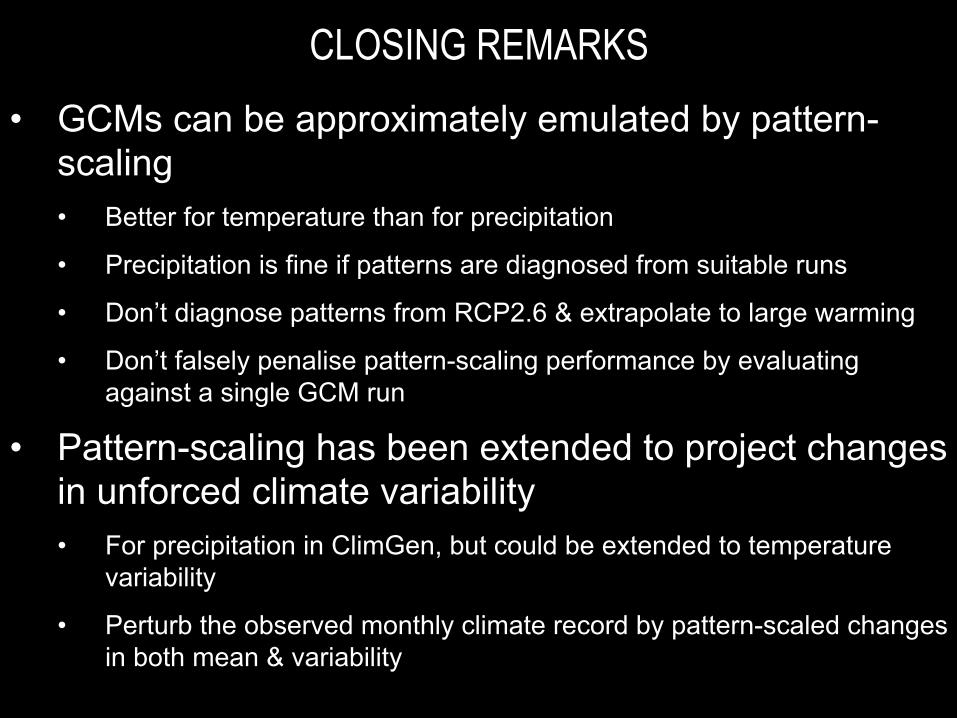
CLOSING REMARKS

•  GCMs can be approximately emulated by pattern-scaling •  Better for temperature than for precipitation

•  Precipitation is fine if patterns are diagnosed from suitable runs

•  Don’t diagnose patterns from RCP2.6 & extrapolate to large warming

•  Don’t falsely penalise pattern-scaling performance by evaluating against a single GCM run

•  Pattern-scaling has been extended to project changes in unforced climate variability •  For precipitation in ClimGen, but could be extended to temperature

variability

•  Perturb the observed monthly climate record by pattern-scaled changes in both mean & variability