UAV Flight Test System

Submitted by

Fong Ming Yang Eugene

U076621U

Department of Mechanical Engineering

In partial fulfillment of the requirements for the Degree of

Bachelor of Engineering

National University of Singapore

Session 2007/2008

2

Summary

The objective of this project is to design and implement a low-cost autopilot system

and study the feasibility and robustness of this autopilot system. The autopilot system

consisted of a navigation subsystem, wireless telemetry subsystem and microcontroller.

Commercial off-the-shelf components meeting budget requirements were carefully chosen

based on inter-operability and performance.

These subsystem components were integrated together and tested rigorously before

flight. The various tests included longitudinal static stability test, electromagnetic

interference, vibration damping and static GPS precision tests. The system was then

integrated on a foam model aircraft.

In addition, original Matlab algorithms were written and refined to cope with the large

amount of flight data. The Matlab algorithms were crucial for streamlining data and quick

results in data analysis.

Eleven separate flight tests were conducted over a period of 6 months and amounted

to extensive experimental data. Ultimately, these data and effort succeeded in achieving

autonomous stabilization and autonomous navigation.

The Ziegler-Nichols gain tuning method was employed for tuning the autonomous

roll and pitch controller for best response. From this method, the flight test system was

successfully tuned to fly straight and level autonomously. The navigation system was also

successfully implemented. Together, the autopilot and navigation proved capable in guiding

the aircraft to a target destination.

3

Acknowledgement

The author wishes to express sincere appreciation to Professor Gerard Leng for his unfailing

support and constant guidance throughout this project. The technicians and support staff of

Dynamics Laboratory have also been an important help. He is also extremely grateful to

Glendon Low for providing the model aircraft and piloting the aircraft during the flight tests.

4

Table of Contents

Summary ................................................................................................................................................................ ............... 2

Acknowledgement.............................................................................................................................................................. 3

List of figures ....................................................................................................................................................................... 6

List of tables ................................................................................................................................................................ ......... 7

List of symbols ................................................................................................................................................................ .... 8

1. Introduction .............................................................................................................................................................. 9

2. Designing the flight test (autopilot) system ............................................................................................... 11

3. Choice of components ........................................................................................................................................ 12

3.1 Microcontroller - ArduPilot .................................................................................................................. 12

3.2 Attitude sensor - ArduIMU ................................................................................................................... 12

3.3 Location tracker – ublox 5 GS407 GPS ........................................................................................... 13

a. Dead reckoning ..................................................................................................................... 13

b. Ground based tracking .......................................................................................................... 13

c. Global Positioning Systems tracking .................................................................................... 13

3.4 Telemetry System – Xbee modules ..................................................................................................... 14

4. Integrating the flight test system on model aircraft ............................................................................. 16

4.1 Linking as a flight test system .............................................................................................................. 16

4.2 Mounting transmitting devices to minimize interference ......................................................... 17

4.3 Optimum ArduIMU placement on aircraft .................................................................................... 18

4.3.1 Damping vibration on ArduIMU ............................................................................... 18

4.3.2 Electromagnetic interference (EMI) on ArduIMU .................................................. 19

4.4 Static longitudinal stability requirement ......................................................................................... 19

4.4.1 Measuring the center of gravity with balancing instrument ................................... 20

4.4.2 Calculation of aerodynamic center ............................................................................ 20

4.4.3 Verifying static longitudinal stability ........................................................................ 21

5. Static GPS precision test................................................................................................................................... 22

5.1 Converting GPS DMS units to meters .............................................................................................. 22

5.2 Analysis of static GPS precision .......................................................................................................... 23

6. Designing the telemetry system ..................................................................................................................... 25

6.1 Sampling rate............................................................................................................................................... 25

6.2 Frame rate .................................................................................................................................................... 26

7. Data reduction process using self-written Matlab code ...................................................................... 27

8. Flight test 1: Validating set-up ....................................................................................................................... 28

5

9. Autopilot control theory ................................................................................................................................... 29

10. Gain tuning via Ziegler-Nichols method ............................................................................................... 30

11. Results of Ziegler-Nichols gain tuning (Flight Test 2 to Flight Test 9) .................................... 32

11.1 Tuning autonomous roll controller with Z-N method ................................................................ 32

11.2 Tuning autonomous pitch controller with Z-N method ............................................................ 34

11.3 Flight test 10: Successful autonomous stabilization .................................................................... 35

11.4 Analysis of Z-N gain tuning method .................................................................................................. 36

12. Flight test 11: Proof of autonomous navigation ................................................................................. 37

12.1 Autonomous turnaround ........................................................................................................................ 37

12.2 Rate of turn during autonomous turnaround................................................................................ 38

12.3 Theoretical turning radius ..................................................................................................................... 39

12.4 Actual turning radius compared to theoretical ............................................................................. 40

12.5 Analysis of turning radius ...................................................................................................................... 41

13. Conclusion and recommendations for future work ......................................................................... 43

References................................................................................................................................................................ .......... 45

Appendix 1: Aircraft properties .................................................................................................................................. 46

Appendix 2: Details of components .......................................................................................................................... 47

Appendix 3: Results from vibration machine ......................................................................................................... 48

Appendix 4: Recommended center of gravity relative to aerodynamic center (Russell, 1996) ............. 49

Appendix 5: GroundStation snapshot ....................................................................................................................... 50

Appendix 6: Raw data collected for static GPS test ............................................................................................. 51

Appendix 7: Data sampling interval .......................................................................................................................... 52

Appendix 8: Autonomous circling test 1 ................................................................................................................. 53

Appendix 9: Autonomous circling test 2 ................................................................................................................. 54

Appendix A: Matlab script GPS.m ............................................................................................................................ 55

Appendix B: Matlab script Sort_Telemetry.m ....................................................................................................... 56

6

List of figures Figure 1: Organization of a flight test system .......................................................................... 11Figure 2: Components of the flight test system ....................................................................... 15Figure 3: Schematic of flight test system ................................................................................. 16Figure 4: Xbee TX and GPS positioned on opposite wing ...................................................... 17Figure 5: (left) Inside the belly of the aircraft. (right) Components inside the aircraft ........... 18Figure 6: Locating aircraft CG with a balancing instrument ................................................... 20Figure 7: Calculation of aerodynamic center ........................................................................... 20Figure 8: Center of gravity is 1cm forward of the aerodynamic center, the aircraft is statically stable in the longitudinal direction ........................................................................................... 21Figure 9: Converting GPS Decimal degrees to degrees, minutes, seconds ............................. 22Figure 10: GPS reading scatter over 10 minutes ..................................................................... 23Figure 11: Algorithm to remove incomplete data .................................................................... 27Figure 12: Flight test 1 Maneuver ............................................................................................ 28Figure 13: Block diagram of autonomous roll controller ........................................................ 29Figure 14: Block diagram of autonomous pitch controller ...................................................... 29Figure 15: Roll response curve at 3 different gains. At K=1.5 (blue), sustained oscillation is observed. At K=1.0 (red), the response is fast and stable. ....................................................... 32Figure 16: Cumulative area under the response curve. At K=1.5 (blue), area is steadily increasing. At K=1.0 (red), the area plateau off quickly and the final value is small. ............ 32Figure 17: Pitch response curve at 2 different gains. At K=1.0 (blue), sustained oscillation is observed. At K=0.6 (red), the response is fast and stable. ....................................................... 34Figure 18: Cumulative area under the response curve. At K=1.0 (blue), area is steadily increasing. At K=0.6 (red), the area plateau off quickly and the final value is small ............. 34Figure 19: Roll and pitch response during autonomous stabilization. With good gains selected, the autopilot can maintain stabilised straight and level flight. .................................. 35Figure 20: Flight path showing autonomous navigation through a 180° turn from T= 0 to 11 seconds. The number next to the line shows the altitude. ........................................................ 37Figure 21: Rate of change of yaw angle at fixed bank angle. Repeated flight tests shows a 30°/s change in yaw angle at fixed -40° bank angle. ............................................................... 38Figure 22: Calculation of theoretical turning radius ................................................................ 39Figure 23: (left) Circle 1; reconstructed flight data shows that the aircraft is flying in a large radius of 100 to 200m. (right) Circle 2; reconstructed flight data shows that at higher speed, the radius is larger. ................................................................................................................... 40Figure 24: Variation of speed for Circle 1 (top graph); Variation of speed for Circle 2 (lower graph). ...................................................................................................................................... 41Figure 25: Flight path change due to side slip ......................................................................... 42

7

List of tables

Table 1: Comparison of IMUs…………………………………………………….. 12 Table 2: Latitude and longitude conversion to meters…………………………...... 22 Table 3: Parameters recorded by telemetry system……………………………….. 26 Table 4: Ziegler-Nichols frequency response method (based on Ku and tu)………. 31

8

List of symbols

φ Roll angle

θ Pitch angle

ψ Yaw angle

W Weight of aircraft

S Surface area of aircraft

Vc Cruise speed

Kp Proportional gain

Ki Integral gain

Kd Derivative gain

Ku Ultimate gain

tu Ultimate period

T Time

9

1. Introduction

Unmanned aerial vehicles (UAVs) have become an integral part of the military in the

recent years. Besides providing numerous advantages, one important capability of UAVs is

the autonomous flying capability. With autonomous flight capability, the aircraft requires

much less manpower, cost and induce less risk to human lives (Barnes, 2009).

While UAVs are a mainstay in the military, there are also many potential applications of

UAVs to civil and commercial circles including aerial photography, coastal surveillance and

agriculture planning (Austin, 2010). However, due to high cost and complexity, adoption of

UAVs outside the military has been slow and cautious (Timothy, 2004; Volpe Center, 2003).

This project aims to study the feasibility of using low-cost, commercial off-the-shelf

components in developing the autonomous capability. The current level of maturity of the

commercial components will be studied and in relation, the deployment of commercial UAVs

can be accelerated.

In truth, a UAV is really part of a larger unmanned aerial system (UAS). The UAS will

consists of some of the following or more: a control station housing the operators, the

aircraft(s) configurable to different type of payloads, a system of communication between

aircraft and operator, and other observers, and support equipment for maintenance and

support (Austin, 2010).

For our project purposes, the autopilot system being designed and implemented will be on

a smaller scale with essential necessities. The basic autopilot system will comprise of a

navigation subsystem, telemetry subsystem, onboard microcontroller and ground control

station.

10

The components that make up the autopilot system are selected based on inter-operability,

cost and effectiveness. These components are commercially available in Singapore. The

system is integrated on a foam model aircraft (Appendix 1).

After integrating the components together as one functioning system onboard the model

aircraft, functional checks were conducted. Once proven airworthy, flight tests were

conducted to determine the best gains in the control laws within the autonomous control

function. The gain tuning method is guided by the Ziegler-Nichols method but were chosen

based on data analysis. Original Matlab codes were also written to cope with the large

amount of data and help in post flight analysis.

The results obtained proved that through extensive flight tests, the flight test system is

able to execute autonomous stabilization and autonomous navigation. This will mean that the

UAV technology built from commercial components have a great potential.

11

2. Designing the flight test (autopilot) system

A complete flight test system consists of several electronics and sensors components. For

our purposes, the flight test system consisted of the microcontroller, the navigation subsystem

and the telemetry subsystem.

Figure 1: Organization of a flight test system

The microcontroller is the central component, which reads in inputs from pilot’s control,

navigation and telemetry. It also holds the autopilot code that executes the control laws and

computes the commands. The navigation system will require appropriate instruments that can

tell its position and measure its attitude. By tracking the aircraft’s position and maintaining a

stable attitude (orientation in roll, pitch and yaw angles), the aircraft can navigate safely from

point to point. While tracking these parameters, a telemetry system must be incorporated so

that the data can be recorded for further analysis. Together with a ground monitoring station,

a telemetry system allows remote monitoring or measurement. Keeping in mind of the costs,

the next section details the choice components used.

12

3. Choice of components

3.1 Microcontroller - ArduPilot

The ArduPilot is a hardware board programmable with the open-source Arduino software.

Besides being small, light and cheap, the ArduPilot has 4 servo outputs. Our model aircraft

requires 3 servo outputs (2 elevon surfaces and 1 throttle). Having one extra servo output and

more I/O ports that are unused means there is room for expansion in future.

3.2 Attitude sensor - ArduIMU

In general, the attitude of the aircraft (roll, pitch, yaw angles) is determined by an inertial

measurement unit (IMU) that combines readings from gyroscopes and accelerometers. Chao

et al (2010) introduced four classes of IMU: (1) Navigation grade; (2) Tactical grade; (3)

Industrial grade; (4) Hobbyist grade. While it is desirable to use the best IMU, resource

constrains mean that a delicate balance of cost and performance must be kept in mind for this

project. Thus some of the options are as follows:

Table 1: Comparison of IMUs IMU Weight(g) Size (mm) Update rate (Hz) Cost (S$) Microstrain 3DM-GX3 18 44 x 25 x 11 <1000 2405 Xsens Mti-g 68 58 x 58 x 33 <120 > 7000 ArduIMU 6 28 x 39 x 12 <50 157

The ArduIMU was chosen because of its affordable pricing and open-source adaptability.

Moreover, its flat size and low weight allows for use in any lightweight foam model aircraft.

Using open source hardware opens up the option for a wide range of online support and

compatible equipment. The ArduIMU is readily compatible for use with the below ublox 5

GPS.

13

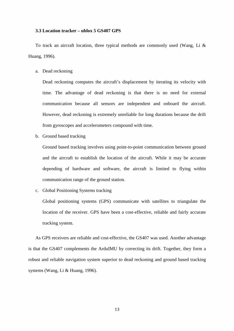
3.3 Location tracker – ublox 5 GS407 GPS

To track an aircraft location, three typical methods are commonly used (Wang, Li &

Huang, 1996).

a. Dead reckoning

Dead reckoning computes the aircraft’s displacement by iterating its velocity with

time. The advantage of dead reckoning is that there is no need for external

communication because all sensors are independent and onboard the aircraft.

However, dead reckoning is extremely unreliable for long durations because the drift

from gyroscopes and accelerometers compound with time.

b. Ground based tracking

Ground based tracking involves using point-to-point communication between ground

and the aircraft to establish the location of the aircraft. While it may be accurate

depending of hardware and software, the aircraft is limited to flying within

communication range of the ground station.

c. Global Positioning Systems tracking

Global positioning systems (GPS) communicate with satellites to triangulate the

location of the receiver. GPS have been a cost-effective, reliable and fairly accurate

tracking system.

As GPS receivers are reliable and cost-effective, the GS407 was used. Another advantage

is that the GS407 complements the ArduIMU by correcting its drift. Together, they form a

robust and reliable navigation system superior to dead reckoning and ground based tracking

systems (Wang, Li & Huang, 1996).

14

3.4 Telemetry System – Xbee modules

Telemetry systems are important as they record aircraft data which are used for analysis.

One can typically have an onboard data logger attached to the aircraft or transmit the data

wirelessly down to a ground station. The advantage of the latter is that operators can view the

data live. Also, an air crash will not compromise on data loss since the data is not stored

onboard the aircraft.

Common wireless transmissions are the radio frequency (RF), Wi-fi 2.4 GHz and

Bluetooth. RF communication can reach long range but are heavily regulated by authorities.

Bluetooth are only used for short range in the order of 10m.

Xbee modules are ideal for this telemetry system because they are light and compact in

size. Using the ZigBee Mesh protocol, the two Xbee modules are synced to communicate on

the 2.4 GHz frequency with a unique network ID. For this project, the 50mW module is

chosen for maximum range. On the aircraft, the Xbee transmitter uses a low profile chip

antenna and is configured as a ‘co-ordinator’ to send serial data continuously. This data will

be picked up by the ground Xbee module (configured as ‘end device’) that has a duck

antenna. This network can be expanded to include more Xbee modules configured as ‘router’

(to relay data) or ‘end device’ so as to expand transmission range.

15

3.5 Summary of components

Figure 2: Components of the flight test system

Literature research has shown that while the above components are not as precise as

military tactical grade instruments, they are sufficiently robust to perform routine missions

and have been successfully implemented to varying degrees (Amahah, 2009; Folkertsma,

2010). Further specifications of the components are attached in Appendix 2.

16

4. Integrating the flight test system on model aircraft

4.1 Linking as a flight test system

As the components were procured separately, the right connections must be done to

function as one system. Since the components work on 5V source which is the same voltage

as RC servos, the power source from the ESC (Electronic Speed Controller) can be tapped.

The schematic of the links in the system is shown.

Figure 3: Schematic of flight test system

In this system, the GPS sends the location data to the ArduIMU. The ArduIMU uses GPS

data to confirm its attitude data. The ArduIMU then sends attitude and location data via serial

data to the ArduPilot. The ArduPilot is the central controller receiving data from sensors and

outputting commands to the elevon servos. It also sends serial data to the Xbee TX, which

forwards them wireless to the ground station. The ArduPilot also acts as an exchange

whereby the pilot can switch between manual to autonomous control anytime. In manual

17

control, the ArduPilot forwards the pilot’s commands to the servos. In autonomous mode, the

ArduPilot computes the commands.

4.2 Mounting transmitting devices to minimize interference

The location of the components on the aircraft can affect performance. The GPS is

mounted at the wing, pointing forward, so that its omni-directional antenna has maximum

line-of-sight connection to satellites over the area, even if the aircraft is upside down. The

Xbee module which transmits data to the ground is mounted on the other wing facing the

ground, so as to establish maximum line-of-sight connectivity to the ground station. Placing

the Xbee module and GPS module on opposite wings helps maintain the centre of gravity on

the centerline of the aircraft. Also, since both modules are transmitting, separating them

minimize interference from each other.

To minimize disruption to the air flow over the wings, the Xbee TX and GPS were

mounted close to the fuselage. As their weights (11g for Xbee TX, 16g for GPS) are similar,

their position will not affect the overall center of gravity much.

Figure 4: Xbee TX and GPS positioned on opposite wing

18

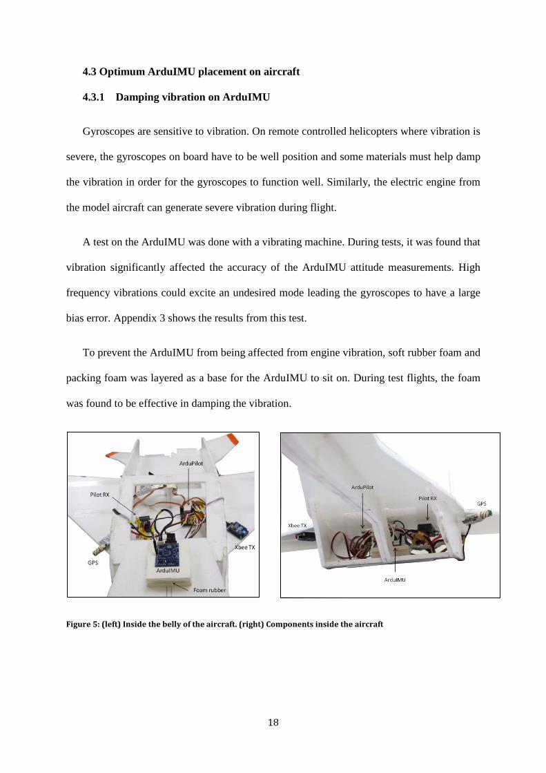
4.3 Optimum ArduIMU placement on aircraft

4.3.1 Damping vibration on ArduIMU

Gyroscopes are sensitive to vibration. On remote controlled helicopters where vibration is

severe, the gyroscopes on board have to be well position and some materials must help damp

the vibration in order for the gyroscopes to function well. Similarly, the electric engine from

the model aircraft can generate severe vibration during flight.

A test on the ArduIMU was done with a vibrating machine. During tests, it was found that

vibration significantly affected the accuracy of the ArduIMU attitude measurements. High

frequency vibrations could excite an undesired mode leading the gyroscopes to have a large

bias error. Appendix 3 shows the results from this test.

To prevent the ArduIMU from being affected from engine vibration, soft rubber foam and

packing foam was layered as a base for the ArduIMU to sit on. During test flights, the foam

was found to be effective in damping the vibration.

Figure 5: (left) Inside the belly of the aircraft. (right) Components inside the aircraft

19

4.3.2 Electromagnetic interference (EMI) on ArduIMU

As the ArduIMU is placed within close proximity of the ESC and motor, EMI is possible.

Excess electromagnetic waves at the right bands can affects the gyroscopes and

accelerometers, since they are based on micro magnetic components.

A test was done to determine whether there is significant EMI on the ArduIMU. Using a

Tri-field meter, it was discovered that upon powering on the motor, the magnetic field

increased from 3 Gauss to more than 100 Gauss. However, the readings from the ArduIMU

remained stable and consistent. The test was repeated by placing the ArduIMU at three

locations: (1) next to motor; (2) on the table far from motor; (3) at center of gravity of the

aircraft. Results showed that the readings were all stable and unaffected.

4.4 Static longitudinal stability requirement

Static stability is the tendency for the aircraft to return to equilibrium position. If the

aircraft is statically stable, a disturbance will generate a correcting moment that tends the

aircraft towards equilibrium position. Without static stability, a disturbance will make the

aircraft spiral out of control.

The most important static stability mode is the longitudinal stability mode (Anderson,

2008). To satisfy this requirement, the center of gravity of the aircraft must be in front of the

aerodynamic center and within the wing (Russell, 1996) (Appendix 4). Before model aircrafts

are flown, the static longitudinal stability is checked to ensure that stable and smooth flights.

20

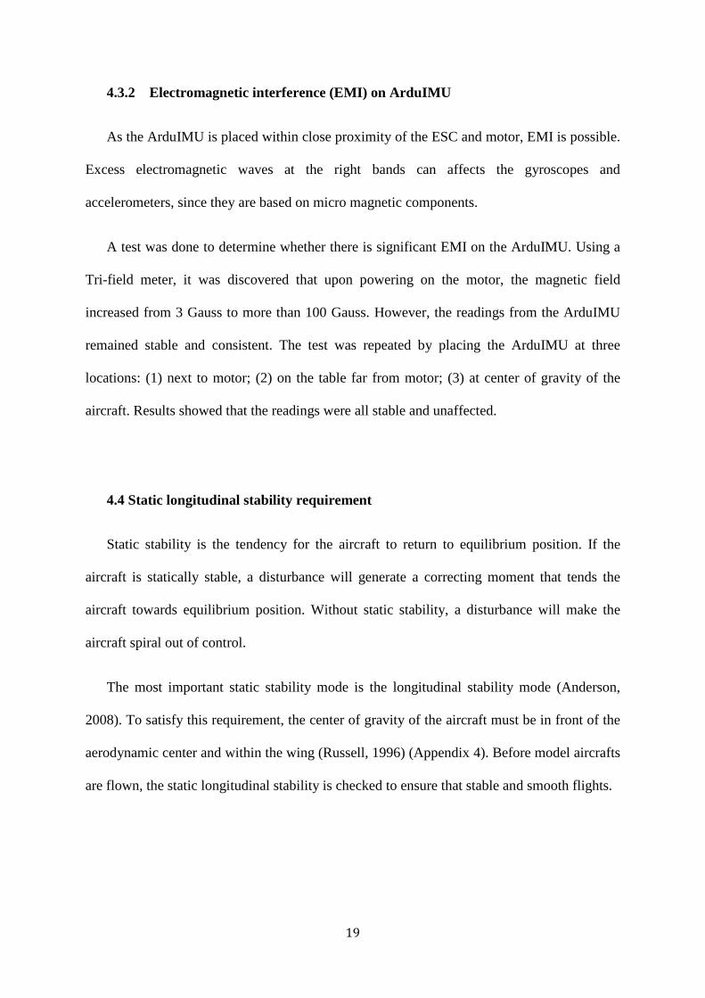
4.4.1 Measuring the center of gravity with balancing instrument

The center of gravity of the aircraft is located using a balancing instrument. Since the

overall weight of the components lies within the longitudinal axis, the center of gravity of the

aircraft still lies within the longitudinal axis. The balancing instrument will locate the point

on the longitudinal axis where the center of gravity lies.

Figure 6: Locating aircraft CG with a balancing instrument

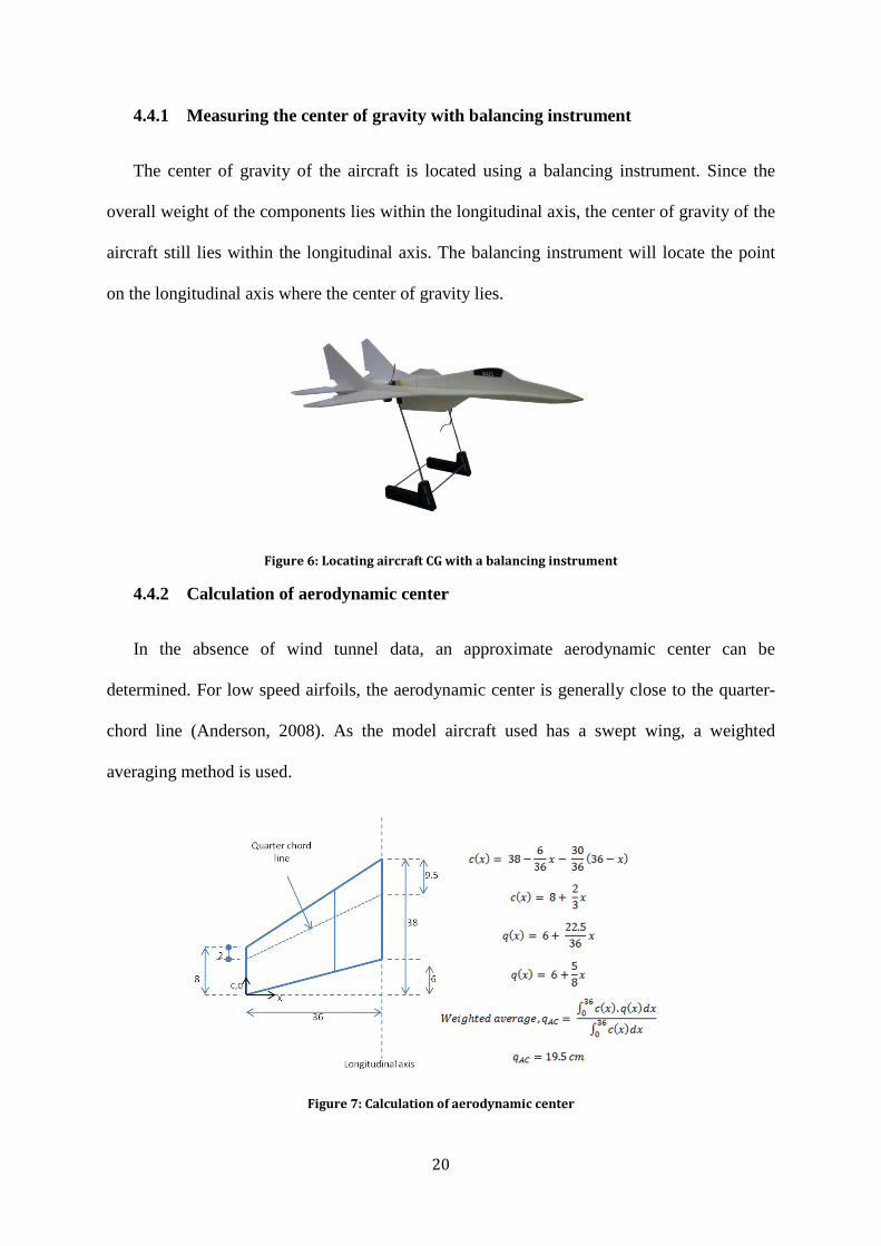
4.4.2 Calculation of aerodynamic center

In the absence of wind tunnel data, an approximate aerodynamic center can be

determined. For low speed airfoils, the aerodynamic center is generally close to the quarter-

chord line (Anderson, 2008). As the model aircraft used has a swept wing, a weighted

averaging method is used.

Figure 7: Calculation of aerodynamic center

21

4.4.3 Verifying static longitudinal stability

From the above results, the center of gravity is 1 cm forward of the aerodynamic center.

This confirms that the aircraft is statically stable in the longitudinal direction.

Figure 8: Center of gravity is 1cm forward of the aerodynamic center, the aircraft is statically stable in the longitudinal direction

22

5. Static GPS precision test

After the avionics components were installed on the plane, a full ground test was

conducted to confirm that all the avionics are functioning and ready for flight. The software

used was the GroundStation. It displays live information of the plane through the Xbee

datalink. The angle read from the GroundStation was verified to the actual angle of the

aircraft. The software also displays the aircraft location superimposed on Google Earth’s

satellite image. The location was correctly pinpointed at E1 block (Appendix 5).

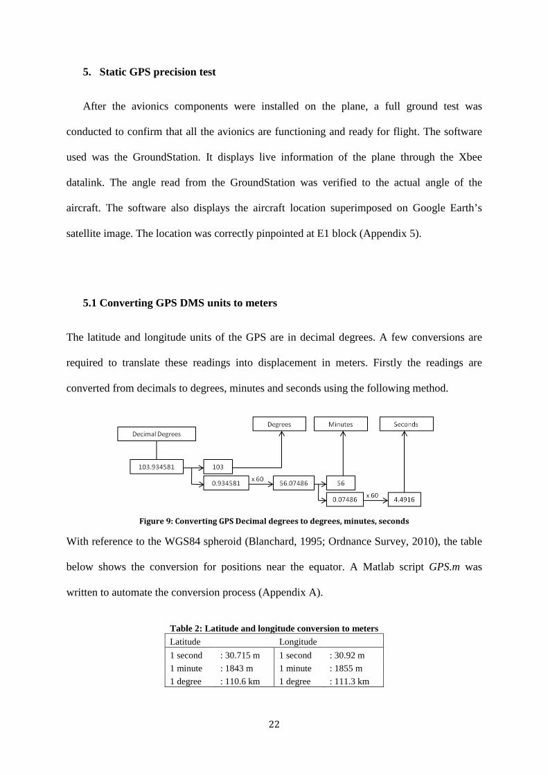
5.1 Converting GPS DMS units to meters

The latitude and longitude units of the GPS are in decimal degrees. A few conversions are

required to translate these readings into displacement in meters. Firstly the readings are

converted from decimals to degrees, minutes and seconds using the following method.

Figure 9: Converting GPS Decimal degrees to degrees, minutes, seconds

With reference to the WGS84 spheroid (Blanchard, 1995; Ordnance Survey, 2010), the table

below shows the conversion for positions near the equator. A Matlab script GPS.m was

written to automate the conversion process (Appendix A).

Table 2: Latitude and longitude conversion to meters Latitude Longitude 1 second : 30.715 m 1 second : 30.92 m 1 minute : 1843 m 1 minute : 1855 m 1 degree : 110.6 km 1 degree : 111.3 km

23

5.2 Analysis of static GPS precision

The GPS was tested in an open area with unobstructed line of sight to the sky on a clear

day. Appendix 6 shows the raw data collected while the plot below shows how the GPS

position changed during a 10 minutes test where the GPS position was fixed. For 2-

dimensional ground location without altitude, the GPS has mean error of 3.33m. For 3-

dimensional location, the mean error is 6.15m.

Figure 10: GPS reading scatter over 10 minutes

The reason why GPS position readings fluctuate are many. In general, GPS location is

calculated based on the time difference of arrival of signals from different satellites. As more

satellites are available, GPS location can be verified with more accuracy. However, satellites

themselves are in constant motion in fixed orbits. Therefore, GPS position readings will

fluctuate accordingly (Blanchard, 1995).

24

Taking the cost limitations in mind, the precision of the 2D GPS can be considered

satisfactory. For better accuracy in altitude in future work, barometer and ultrasound sensors

are recommended.

25

6. Designing the telemetry system

6.1 Sampling rate

The telemetry data are discrete samples of a continuously varying data. For an ideal

system, the sampling rate of the sensor must be at least twice the highest frequency in the

signal (Carden, Jedlicka & Henry, 2002). Due to distortion in the sampling and reconstruction

process, industrial telemetry systems sample at least four times more.

In this aircraft, a typical roll or pitch disturbance introduced during steady level flight will

result in an oscillation in the order of 1 Hz. As such, to describe the oscillation from discrete

step measurements, the attitude data sampling rate should be at least 2 samples per second.

The position data of the plane are not as critical as the attitude. Without fresh position

data, the plane will only risk overshooting a waypoint and will have to circle back. Assuming

a waypoint radius of 50 meters, at cruise speed of 10 meters per second, the plane will be

inside the circle for up to 5 seconds. Thus a position data samples spaced 2.5 seconds apart is

sufficient.

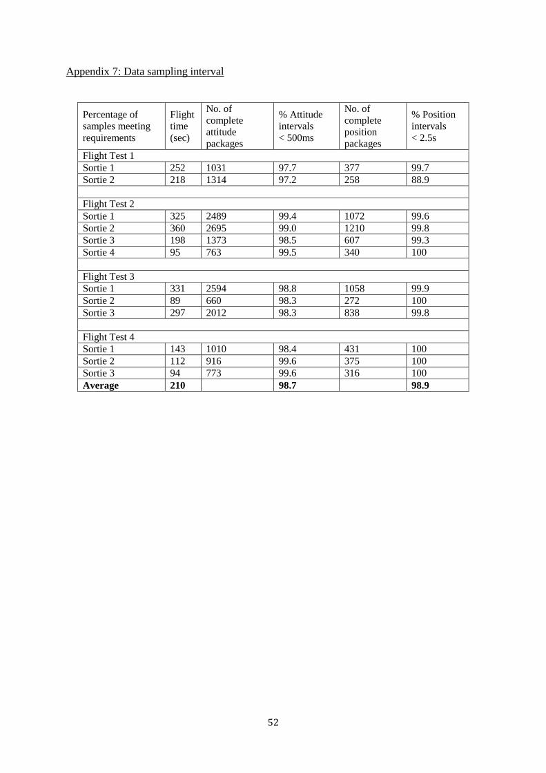
Based on 4 separate flight test data (Flight test 1 to Flight test 4), with average flying time

of about 210 seconds, the telemetry sampling rate met the above requirements. For attitude

sampling rate requiring intervals of less than 500 milliseconds, it was found that 98.7% of the

data met this requirement. For position sampling rate, 98.9% met the requirement for less

than 2.5 seconds apart. Appendix 7 shows the details during each sortie.

26

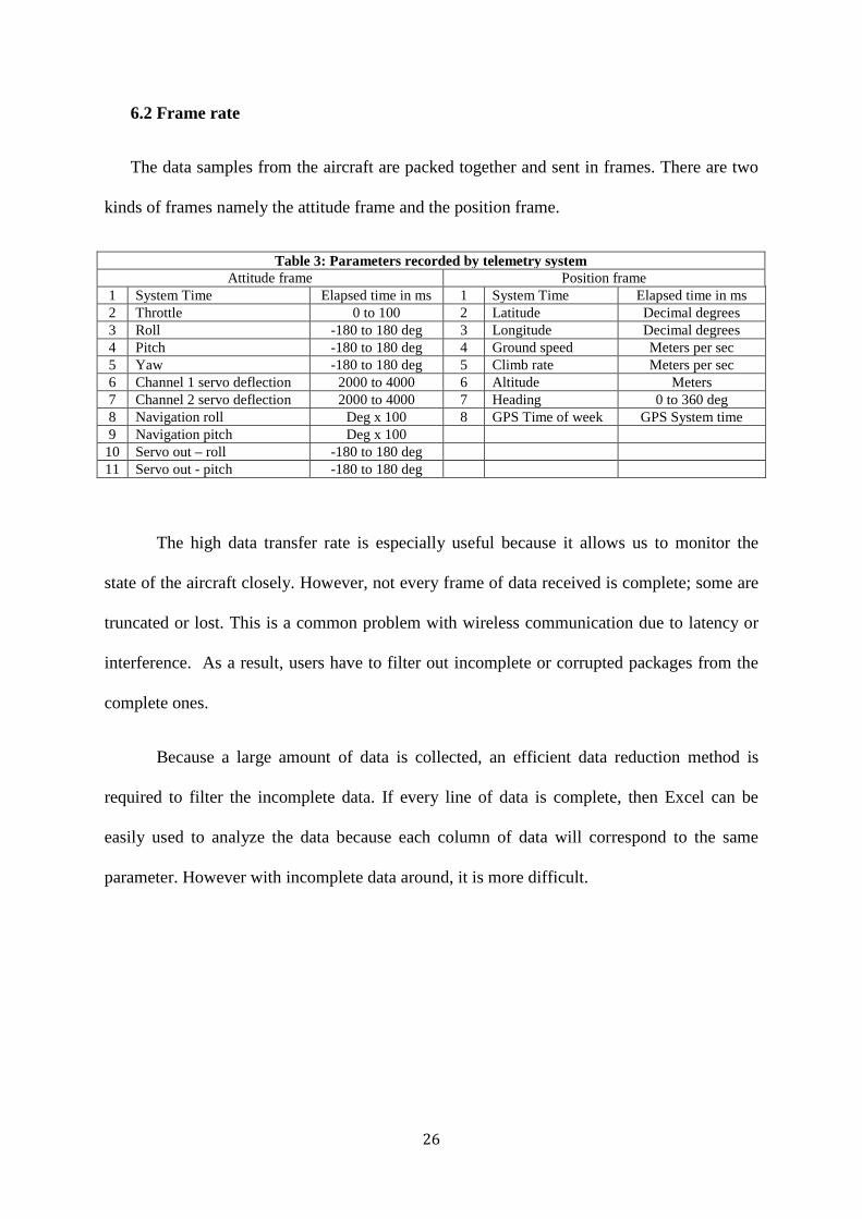
6.2 Frame rate

The data samples from the aircraft are packed together and sent in frames. There are two

kinds of frames namely the attitude frame and the position frame.

Table 3: Parameters recorded by telemetry system Attitude frame Position frame

1 System Time Elapsed time in ms 1 System Time Elapsed time in ms 2 Throttle 0 to 100 2 Latitude Decimal degrees 3 Roll -180 to 180 deg 3 Longitude Decimal degrees 4 Pitch -180 to 180 deg 4 Ground speed Meters per sec 5 Yaw -180 to 180 deg 5 Climb rate Meters per sec 6 Channel 1 servo deflection 2000 to 4000 6 Altitude Meters 7 Channel 2 servo deflection 2000 to 4000 7 Heading 0 to 360 deg 8 Navigation roll Deg x 100 8 GPS Time of week GPS System time 9 Navigation pitch Deg x 100

10 Servo out – roll -180 to 180 deg 11 Servo out - pitch -180 to 180 deg

The high data transfer rate is especially useful because it allows us to monitor the

state of the aircraft closely. However, not every frame of data received is complete; some are

truncated or lost. This is a common problem with wireless communication due to latency or

interference. As a result, users have to filter out incomplete or corrupted packages from the

complete ones.

Because a large amount of data is collected, an efficient data reduction method is

required to filter the incomplete data. If every line of data is complete, then Excel can be

easily used to analyze the data because each column of data will correspond to the same

parameter. However with incomplete data around, it is more difficult.

27

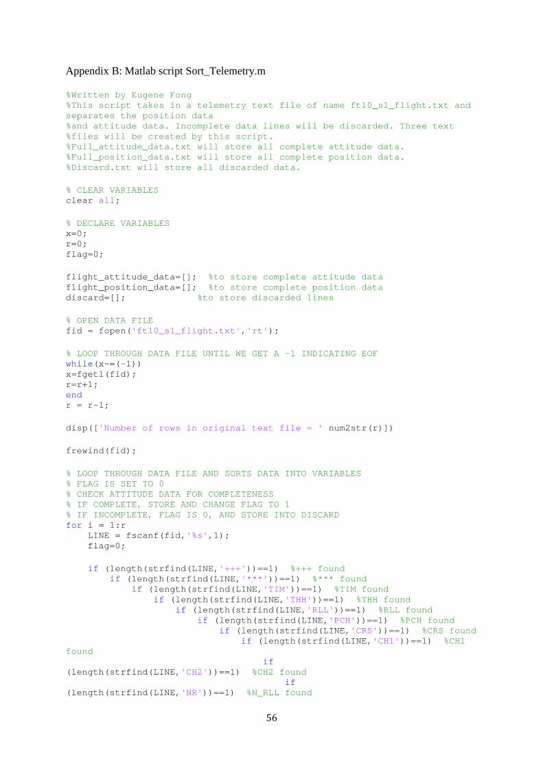
7. Data reduction process using self-written Matlab code

In order to make this filtering process more efficient, a Matlab code Sort_Telemetry.m

(Appendix B) was written. The script reads in the raw telemetry text file and checks each line

for completeness by checking each parameter name. If the line is complete, it is stored. If any

parameters are missing, the line is discarded. Further, the code will automatically store the

complete lines into two separate files - Full_attitude_data.txt and Full_position_data.txt.

According to which frame that line corresponds to, the line will be stored in the correct text

file. In this way, attitude and position data can be easily analyzed separately. Incomplete data

will be stored in discard.txt. This will significantly less time to sort through the thousands of

lines of data.

Figure 11: Algorithm to remove incomplete data

28

8. Flight test 1: Validating set-up

Flight Test 1 was conducted with the aim of verifying the full functionality of the

avionics in flight. The plane was flown in manual mode a few times and performed a steep

climb and the ‘figure of 8’ maneuver. During this maneuver the plane banks hard and is

subjected to sudden forces. This confirms that the avionics are securely strapped on the plane

and that telemetry data are still continuously streaming in even when the plane is under rough

flying conditions. The figure below shows a typical flight path with colors indicating the

altitude.

Figure 12: Flight test 1 Maneuver

29

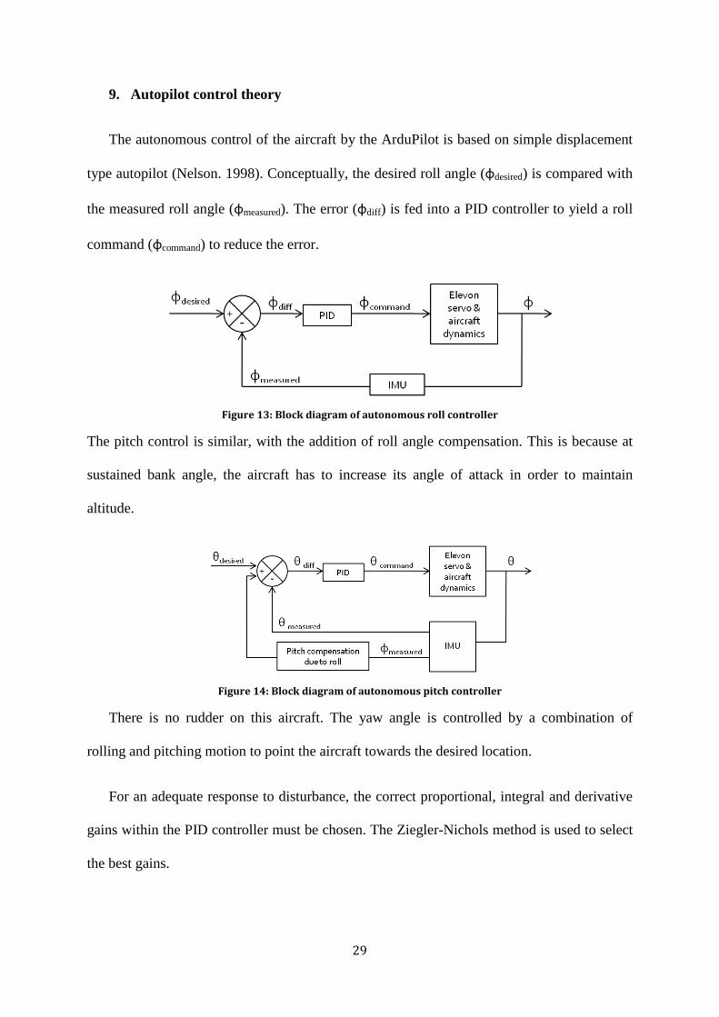
9. Autopilot control theory

The autonomous control of the aircraft by the ArduPilot is based on simple displacement

type autopilot (Nelson. 1998). Conceptually, the desired roll angle (φdesired) is compared with

the measured roll angle (φmeasured). The error (φdiff) is fed into a PID controller to yield a roll

command (φcommand) to reduce the error.

Figure 13: Block diagram of autonomous roll controller

The pitch control is similar, with the addition of roll angle compensation. This is because at

sustained bank angle, the aircraft has to increase its angle of attack in order to maintain

altitude.

Figure 14: Block diagram of autonomous pitch controller

There is no rudder on this aircraft. The yaw angle is controlled by a combination of

rolling and pitching motion to point the aircraft towards the desired location.

For an adequate response to disturbance, the correct proportional, integral and derivative

gains within the PID controller must be chosen. The Ziegler-Nichols method is used to select

the best gains.

30

10. Gain tuning via Ziegler-Nichols method

PID controllers are important tools widely used in automation. A simple PID controller

attempts to minimize error between the process variable and the setpoint by adjusting the

process control inputs. The proportional (P) gain determines the ratio of output response to

error signal. The integral (I) gain sums the error over time, while the derivative (D) gain is

proportional to the rate of change of the process variable.

There are a few methods for tuning the PID gains. In certain industries, specialized

software can simulate the process. The PID gains can be selected through rigorous software

analysis. As this project has limited time and resource constrain, specialized software is not

used. Rather, a heuristical approach based on classical method – the Ziegler-Nichols method -

is employed.

The common compromise for controllers is the dilemma between speed and stability. Fast

control usually leads to oscillations while a stable control is sluggish. Thus the most common

compromise is to adjust the controller so that the response curve has a quarter decay (Tan,

Wang & Hang, 1999).

The Ziegler-Nichols frequency response method is designed for quarter decay and

evaluates a system at the limit of stability. Despite simple mathematical rules, history has

shown that has worked well for many applications and is the basis for modern process control

methods.

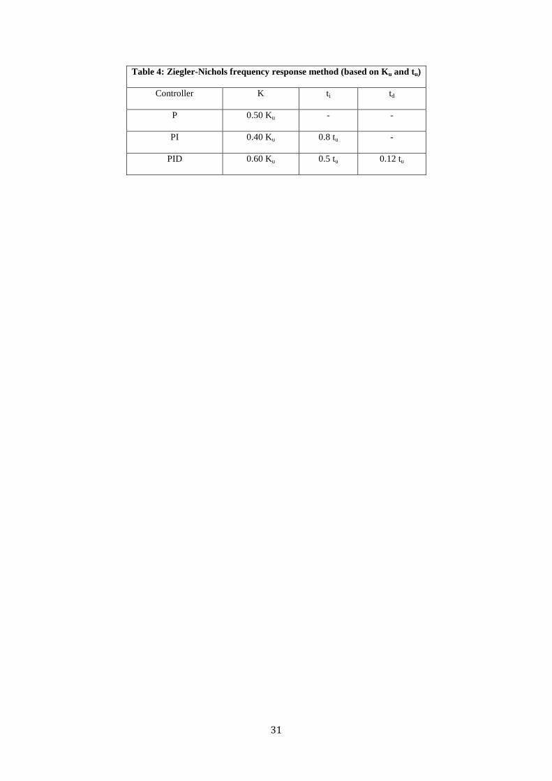
Employing the Ziegler-Nichols method, results can be quickly obtainable through

repeated experiments. The method involves trying out several P gains until the process

variable oscillate with a constant period, tu. This gain, called the ultimate gain Ku, can be used

to directly select the best PID gains based on the table below (Aström & Häggland, 1988).

31

Table 4: Ziegler-Nichols frequency response method (based on Ku and tu)

Controller K ti td

P 0.50 Ku - -

PI 0.40 Ku 0.8 tu -

PID 0.60 Ku 0.5 tu 0.12 tu

32

11. Results of Ziegler-Nichols gain tuning (Flight Test 2 to Flight Test 9)

The Ziegler-Nichols gain tuning method was executed over a period of 9 separate flight

tests. For this part of the test, the aircraft was flown in Stabilise mode. In this mode, the

ArduPilot autonomously maintains the aircraft level and straight (φdesired=0 and θdesired=0).

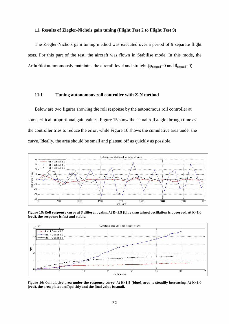
11.1 Tuning autonomous roll controller with Z-N method

Below are two figures showing the roll response by the autonomous roll controller at

some critical proportional gain values. Figure 15 show the actual roll angle through time as

the controller tries to reduce the error, while Figure 16 shows the cumulative area under the

curve. Ideally, the area should be small and plateau off as quickly as possible.

Figure 15: Roll response curve at 3 different gains. At K=1.5 (blue), sustained oscillation is observed. At K=1.0 (red), the response is fast and stable.

Figure 16: Cumulative area under the response curve. At K=1.5 (blue), area is steadily increasing. At K=1.0 (red), the area plateau off quickly and the final value is small.

33

Based on flight test results, the approximate ultimate gain for the roll controller is Ku =

1.5. At K=1.5, Figure 15 shows that the controller causes an oscillation in the roll angle.

Furthermore, Figure 16 shows the cumulative area under the curve to be increasing linearly,

indicating a relatively symmetric oscillation.

The Z-N method then recommends K=0.8, which results in a better response for the roll

controller. Figure 16 shows that at K=0.8, the cumulative area plateau near the 10th data

point.

However, closer analysis reveals that K=0.8 is not the optimum gain value for the roll

controller. Figure 15 shows that the roll angle is still oscillating significantly until the 2000ms

mark. Tests reveal that K=1.0 is a better gain value and the above figure shows the marked

improvement. At K=1.0, Figure 15 shows the roll controller is able to control the roll angle

very well near the desired roll angle of zero, and figure 16 shows the cumulative area to be

lesser and it plateau off at the 5th data point.

Therefore, based on these experimental tests, the roll controller is able to keep the roll

angle at desired setting best with a proportional gain of 1.0.

34

11.2 Tuning autonomous pitch controller with Z-N method

Figure 17: Pitch response curve at 2 different gains. At K=1.0 (blue), sustained oscillation is observed. At K=0.6 (red), the response is fast and stable.

Figure 18: Cumulative area under the response curve. At K=1.0 (blue), area is steadily increasing. At K=0.6 (red), the area plateau off quickly and the final value is small

The experience from tuning the roll controller tell us that the Z-N method tend to

underestimate a good gain value. From tests, the ultimate gain for pitch controller is K=1.0.

Again Figure 18 shows a approximate linearly increasing area.

In tuning the pitch controller, it is found that a gain of K=0.6 performs very well. The

pitch controller maintains the desired angle most of the time and the area under the curve is

small and plateau off at the 9th data point.

35

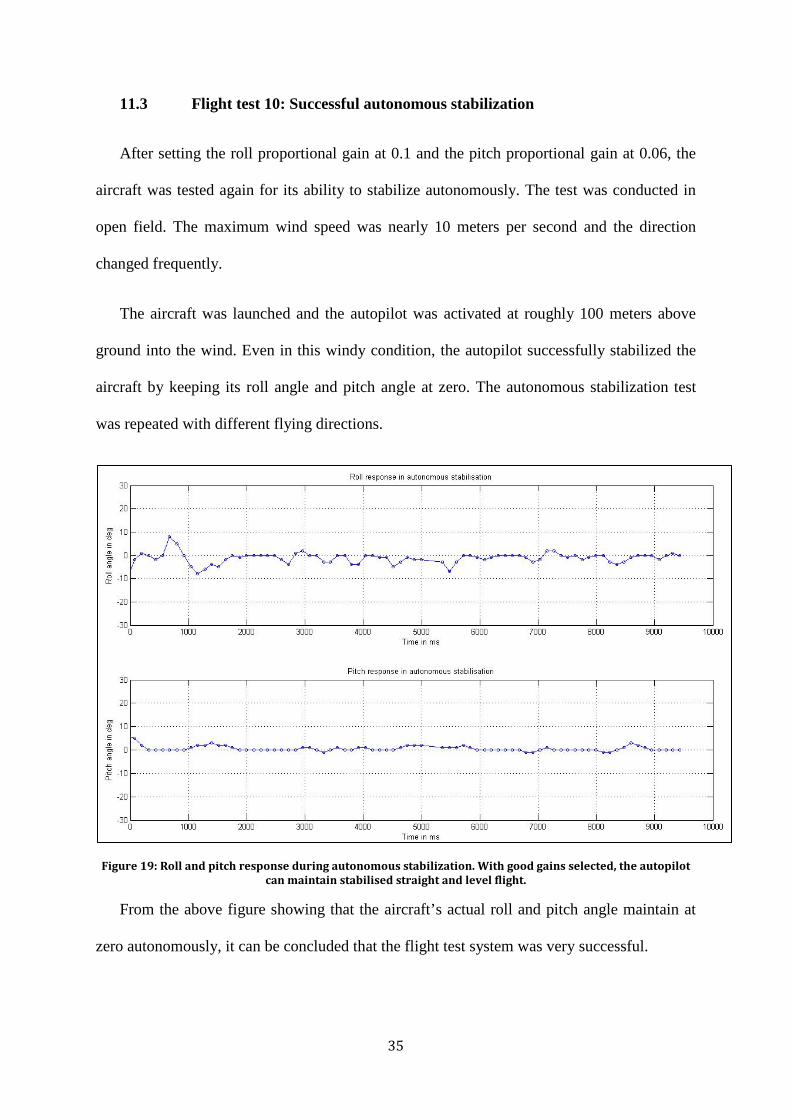
11.3 Flight test 10: Successful autonomous stabilization

After setting the roll proportional gain at 0.1 and the pitch proportional gain at 0.06, the

aircraft was tested again for its ability to stabilize autonomously. The test was conducted in

open field. The maximum wind speed was nearly 10 meters per second and the direction

changed frequently.

The aircraft was launched and the autopilot was activated at roughly 100 meters above

ground into the wind. Even in this windy condition, the autopilot successfully stabilized the

aircraft by keeping its roll angle and pitch angle at zero. The autonomous stabilization test

was repeated with different flying directions.

Figure 19: Roll and pitch response during autonomous stabilization. With good gains selected, the autopilot can maintain stabilised straight and level flight.

From the above figure showing that the aircraft’s actual roll and pitch angle maintain at

zero autonomously, it can be concluded that the flight test system was very successful.

36

11.4 Analysis of Z-N gain tuning method

The Z-N gain tuning method has proven to be a quick and reliable method in determining

the gains for the autopilot controller. However, the gains predicted via the Z-N method tend

to underestimate a good gain value.

The reason is because the basis of the Z-N method is to attain a quarter decay amplitude

in the response curve. For our system, a quarter decay amplitude is too sluggish.

In this system, the aircraft is airborne and reacting to external disturbances from wind.

Because of the unpredictable wind strength and direction, the aircraft is subjected to varying

disturbances. A sluggish albeit stable response will be insufficient because by the time the

aircraft has damped the initial disturbance, another disturbance of different nature will be in

effect. Moreover, a slow response may mean a large change in angle of attack or altitude,

both of which may lead to unstable and undesirable aerodynamic conditions resulting in a

crash.

Therefore for this system, a more reactive and sensitive response is preferred. As such a

higher than predicted gain has proven to be better. While overshoot was acceptable, extreme

care was taken not to increase the gain too much so as not to introduce prolonged oscillations.

37

12. Flight test 11: Proof of autonomous navigation

12.1 Autonomous turnaround

Next, the partial autonomous navigation was tested via the Return to Launch (RTL)

mode. The aircraft was launched and was steered so that it is moving away from target

destination. The autopilot was then engaged and the aircraft turns around autonomously.

Figure 20: Flight path showing autonomous navigation through a 180° turn from T= 0 to 11 seconds. The

number next to the line shows the altitude.

Upon autopilot activation, the autopilot controller sent a roll command angle of -40

degrees. This successfully proves that the navigation system is aware of the aircraft’s location

relative to target destination. Within two seconds, the actual roll angle meets the commanded

roll angle and the aircraft begins a turn. Between T=7s to T=9s, the autopilot controller

attempts to bring the aircraft back level. At T=11s, a roll command of 20 degrees was

commanded so that the aircraft will be heading directly to target destination. Throughout the

maneuver, the altitude was in the safe region of 77±10 m.

38

In summary, the aircraft was able to make a sustained turn successfully without losing

altitude and stability.

12.2 Rate of turn during autonomous turnaround

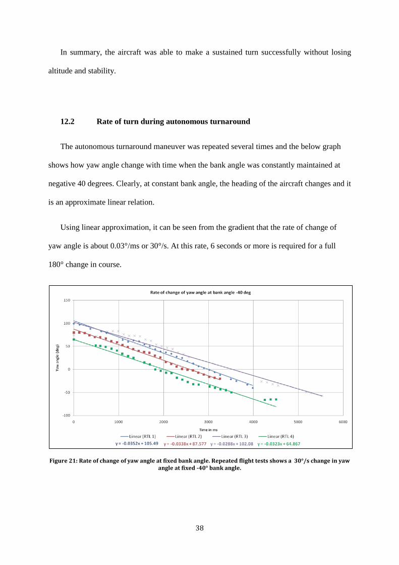
The autonomous turnaround maneuver was repeated several times and the below graph

shows how yaw angle change with time when the bank angle was constantly maintained at

negative 40 degrees. Clearly, at constant bank angle, the heading of the aircraft changes and it

is an approximate linear relation.

Using linear approximation, it can be seen from the gradient that the rate of change of

yaw angle is about 0.03°/ms or 30°/s. At this rate, 6 seconds or more is required for a full

180° change in course.

Figure 21: Rate of change of yaw angle at fixed bank angle. Repeated flight tests shows a 30°/s change in yaw angle at fixed -40° bank angle.

39

12.3 Theoretical turning radius

Using the above information, we can estimate how fast the aircraft can change its course

at a sustained bank angle.

Assuming a steady, level, co-ordinated turn at bank angle 40°, the theoretical turning

radius can be calculated based on constant cruise speed, vc. To make a 180° change in course

in a co-ordinated turn, the distance traversed by the aircraft is half the circumference (πr).

The time taken to change its course is approximately the time taken to cover the distance.

𝑡 =𝜋𝑟𝑣𝑐

=18030

= 6

𝑟 =6𝑣𝑐𝜋

Figure 22: Calculation of theoretical turning radius

40

12.4 Actual turning radius compared to theoretical

The next step was to analyze the aircraft’s ability to circle autonomously. In the first test,

Circle 1 (see figure below, left), the average cruise speed was 15 meters per second

(Appendix 8 shows the flight data). At this speed, the calculated theoretical turning radius is

30 meters. However, the flight path generated from the GPS data shows the aircraft is unable

to sustain this tight radius.

In the second test, Circle 2 (see figure below), right, the average cruise speed was 20

meters per second (Appendix 9) and the theoretical turning radius is 40 meters. By

reconstructing the flight path from the telemetry data, it can be seen that the aircraft is unable

to steadily subscribe within the theoretical radius. Also, at higher speeds, the aircraft tends to

have a larger radius as predicted by the formula.

Figure 23: (left) Circle 1; reconstructed flight data shows that the aircraft is flying in a large radius of 100 to 200m. (right) Circle 2; reconstructed flight data shows that at higher speed, the radius is larger.

41

12.5 Analysis of turning radius

a. GPS errors

In both cases, the aircraft was unable to completely subscribe to a perfect circle or meet

the theoretical turning radius. One reason is that the radius and launch location is defined by

GPS co-ordinates. GPS co-ordinates are not precise and as discussed before, GPS co-

ordinates drift in the order of several meters. However, the error of several meters should not

result in a turning radius more than two or three times the expected as shown.

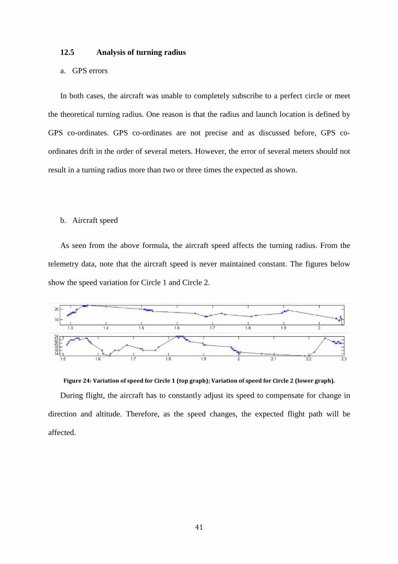
b. Aircraft speed

As seen from the above formula, the aircraft speed affects the turning radius. From the

telemetry data, note that the aircraft speed is never maintained constant. The figures below

show the speed variation for Circle 1 and Circle 2.

Figure 24: Variation of speed for Circle 1 (top graph); Variation of speed for Circle 2 (lower graph).

During flight, the aircraft has to constantly adjust its speed to compensate for change in

direction and altitude. Therefore, as the speed changes, the expected flight path will be

affected.

42

c. Wind conditions

In addition, the actual velocity of the aircraft is greatly affected by the wind as well.

During the test flight, wind speed was about 10 meters per second. This is significant

compared to the aircraft speed. The consequence is that the wind direction can cause the

aircraft to side-slip, thus changing the instantaneous velocity vector. With significant side-

slip, the aircraft will need a longer time and travel a longer distance as illustrated below.

Figure 25: Flight path change due to side slip

In real conditions, it is very difficult to maintain the speed at a fixed value since the wind

conditions is varying and unpredictable. As a result, the aircraft will most likely have to make

large adjustments to its course and bank angle constantly.

43

13. Conclusion and recommendations for future work

This project has successfully achieved its objective of designing and implementing a

flight test system using low-cost, commercial-of-the-shelf components. Through rigorous

selection criteria, the best components for the navigation system, telemetry system and

controller were used. More importantly, these separate components were successfully

integrated as one complete system onto the model aircraft.

After the integrated system has proved functional on the ground, critical tests and

evaluations were done before the aircraft was ready for flight tests. Static longitudinal

stability, electromagnetic interference, vibration damping and the static GPS test all served to

ensure the system will deliver optimum data.

Through such critical preparation, Flight Test 1 was successfully executed. The Matlab

algorithms were crucial is streamlining data and quick post flight analysis. From Flight Test 2

to Flight Test 9, gain tuning of the autopilot controllers was guided by the Ziegler-Nichols

method. Results show that the roll controller performed best with a proportional gain of 1.0

while the pitch controller performed best at 0. 6.

On Flight Test 10, the aircraft successfully executed autonomous straight and level flight.

Even under unpredictable gusty weather conditions, the autopilot was proven to be reliable

and stable.

During Flight Test 11, autonomous navigation was tested rigorously by executing an

autonomous turnaround. The autopilot successfully steered the aircraft to target destination

through a 180° degree change in heading. During this maneuver, the bank angle was

consistently maintained by the controller and the aircraft performed a level turn. Results

showed that at bank angle of -40 degrees, the rate of change of yaw is about 30°/sec.

44

Depending on cruise speed vc, the theoretical minimum radius is 𝑟 = 6𝑣𝑐𝜋

. The actual turning

radius is affected by many factors such as wind speed, wind direction and GPS accuracy.

My recommendations for future work would be to include a more sensitive sensor for

measuring altitude. For example, barometer or long range ultra-sound sensors can give more

precise altitude measurements. With improved altitude sensor, the aircraft can conduct a

better level turn. A better GPS sensor will also improve location tracking and autonomous

navigation performance.

As this aircraft used is a light-weight foam aircraft, it is very sensitive to wind conditions.

As such, executing maneuvers like turning and navigation can take longer than predicted due

to adverse wind forces. Large sideslip was often the case during our test flights. By using a

wooden aircraft of more mass, it will be less susceptible to wind conditions and will be able

to execute more precise maneuvers.

To advance into the bigger aim of putting UAVs into civil and commercial use, the

autopilot must be capable of autonomous take-off and landing. The aircraft used here was

hand launched and landed on its belly. The next step forward would be to use a more typical

aircraft with wheels, and test and implement autonomous take-off and landing algorithms.

45

References 1. Barnes, O. (2009). Air Power: UAVs: The wider context. Royal Air Force Centre for

Air Power Studies

2. Austin, R. (2010). Unmanned Aircraft Systems – UAVS Design, development and

deployment. John Wiley & Sons, Ltd.

3. Timothy H. Cox et al. (2004). Civil UAV Capability Assessment. NASA.

4. Volpe Center; NCRST-Infrastructure. (2003, December 2). A Roadmap for deploying

UAV in Transportation

5. Chao H., Coopmans C., Long D., & Chen Y. (2010). A comparative evaluation of low

cost IMUs for unmanned autonomous systems. 2010 IEEE International Conference

on Multisensor Fusion and Integration for Intelligent Systems (MFI 2010), 211-16.

6. Wang Y., Li X. & Huang Y. (1996). Navigation system of pilotless aircraft via GPS.

IEEE Aerospace and Electronics Systems Magazine, v 11, n 8, 16-20, Aug. 1996.

7. Amahah, J. (2009). The design of an unmanned aerial vehicle based on the ArduPilot.

Georgian Electronic Scientific Journal: Computer science and telecommunications

2009 No. 5(22).

8. Folkertsma, G. (2010). Unmanned aerial vehicles: modeling and control of a

miniature helicopter. University of Twente.

9. Russell, J.B. (1996). Performance and stability of aircraft. New York. Wiley.

10. Anderson, J.D.(Jr) (2008). Introduction to flight. McGraw Hill.

11. Blanchard, W. (1995). The air pilot’s guide to satellite positioning system. Airlife

Publishing.

12. (2010). A guide to coordinate systems in Great Britain. Ordnance Survey.

13. Nelson, R. (1998). Flight stability and automatic control. McGraw-Hill International

Editions.

14. Tengku, L.T.M., Raimi, H.A.M. & Zulkifli, M. (2010). Development of Auto Tuning

PID Controller using Graphic User Interface (GUI). 2010 Second International

Conference on Computer Engineering and Applications.

15. Tan, K.K., Wang, Q.G. & Hang, C.C. (1999). Advances in PID Control. Great

Britain. Springer-Verlag London Limited 1999.

16. Aström, K.J. & Hägglund, T. (1988). Automatic Tuning of PID Controllers. United

States of America. Instrument Society of America 1988.

17. Carden, F., Jedlicka, R. & Henry, R. (2002). Telemetry Systems Engineering.

Norwood. Artech House, Inc.

46

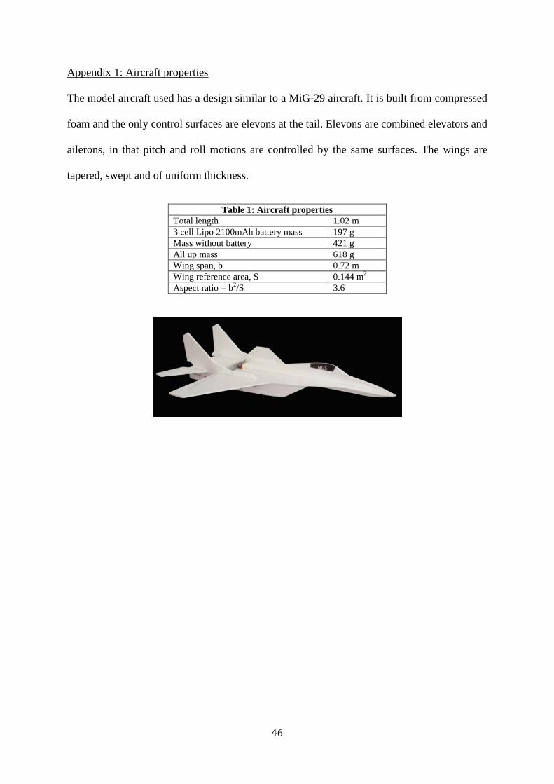
Appendix 1: Aircraft properties

The model aircraft used has a design similar to a MiG-29 aircraft. It is built from compressed

foam and the only control surfaces are elevons at the tail. Elevons are combined elevators and

ailerons, in that pitch and roll motions are controlled by the same surfaces. The wings are

tapered, swept and of uniform thickness.

Table 1: Aircraft properties Total length 1.02 m 3 cell Lipo 2100mAh battery mass 197 g Mass without battery 421 g All up mass 618 g Wing span, b 0.72 m Wing reference area, S 0.144 m2 Aspect ratio = b2/S 3.6

47

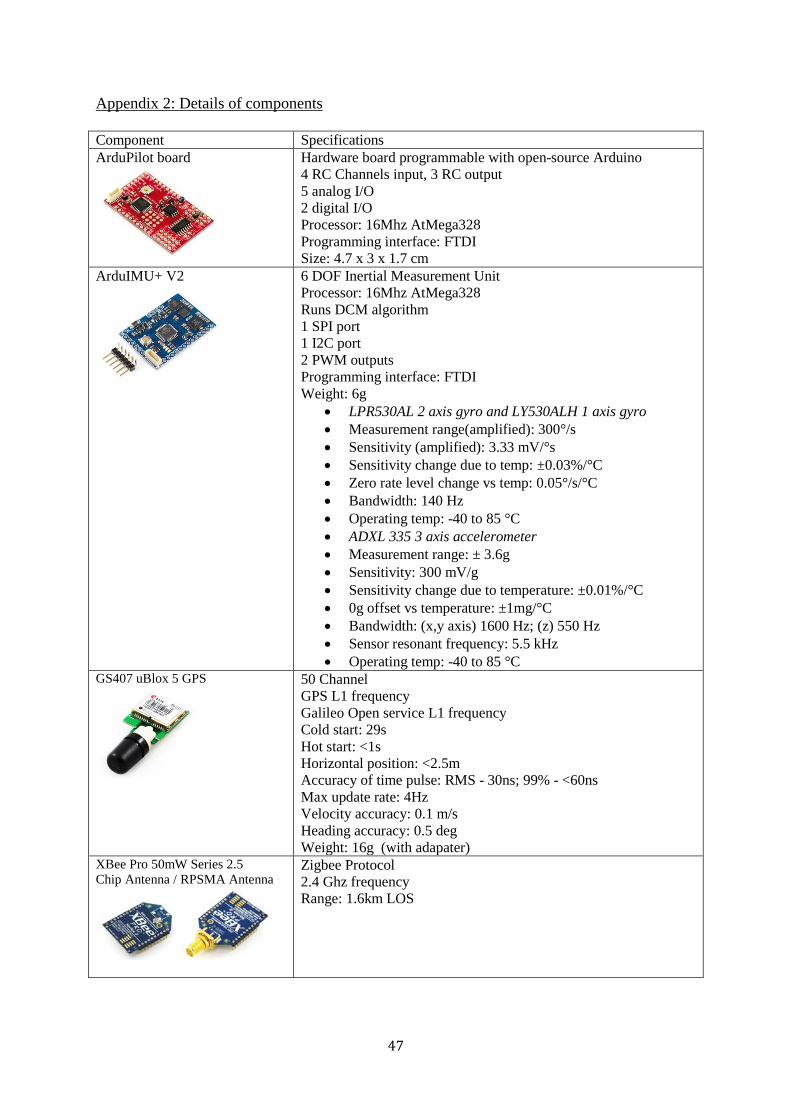
Appendix 2: Details of components

Component Specifications ArduPilot board

Hardware board programmable with open-source Arduino 4 RC Channels input, 3 RC output 5 analog I/O 2 digital I/O Processor: 16Mhz AtMega328 Programming interface: FTDI Size: 4.7 x 3 x 1.7 cm

ArduIMU+ V2

6 DOF Inertial Measurement Unit Processor: 16Mhz AtMega328 Runs DCM algorithm 1 SPI port 1 I2C port 2 PWM outputs Programming interface: FTDI Weight: 6g

• LPR530AL 2 axis gyro and LY530ALH 1 axis gyro • Measurement range(amplified): 300°/s • Sensitivity (amplified): 3.33 mV/°s • Sensitivity change due to temp: ±0.03%/°C • Zero rate level change vs temp: 0.05°/s/°C • Bandwidth: 140 Hz • Operating temp: -40 to 85 °C • ADXL 335 3 axis accelerometer • Measurement range: ± 3.6g • Sensitivity: 300 mV/g • Sensitivity change due to temperature: ±0.01%/°C • 0g offset vs temperature: ±1mg/°C • Bandwidth: (x,y axis) 1600 Hz; (z) 550 Hz • Sensor resonant frequency: 5.5 kHz • Operating temp: -40 to 85 °C

GS407 uBlox 5 GPS

50 Channel GPS L1 frequency Galileo Open service L1 frequency Cold start: 29s Hot start: <1s Horizontal position: <2.5m Accuracy of time pulse: RMS - 30ns; 99% - <60ns Max update rate: 4Hz Velocity accuracy: 0.1 m/s Heading accuracy: 0.5 deg Weight: 16g (with adapater)

XBee Pro 50mW Series 2.5 Chip Antenna / RPSMA Antenna

Zigbee Protocol 2.4 Ghz frequency Range: 1.6km LOS

48

Appendix 3: Results from vibration machine

The ArduIMU was initialized at zero degree roll and pitch. The table below shows the change in sensor readings in the roll and pitch at different frequencies and gain.

Frequency Gain Pitch Roll 80 Hz 2 0 0

6 1.8 0.3 10 6.2 0.9

90 Hz 2 0.2 0.1

6 1 0.3 10 4.1 0.5

100 Hz 2 0.3 0

6 0.5 0.2 10 1.5 0.3

110 Hz 2 0.3 0

6 2.1 0.2 10 5 0.5

120 Hz 2 0.2 0

6 4.3 0.3 10 7 0

130 Hz 2 0.3 0

6 2.9 0.1 10 4.5 0.3

49

Appendix 4: Recommended center of gravity relative to aerodynamic center (Russell, 1996)

50

Appendix 5: GroundStation snapshot

51

Appendix 6: Raw data collected for static GPS test

52

Appendix 7: Data sampling interval

Percentage of samples meeting requirements

Flight time (sec)

No. of complete attitude packages

% Attitude intervals < 500ms

No. of complete position packages

% Position intervals < 2.5s

Flight Test 1 Sortie 1 252 1031 97.7 377 99.7 Sortie 2 218 1314 97.2 258 88.9 Flight Test 2 Sortie 1 325 2489 99.4 1072 99.6 Sortie 2 360 2695 99.0 1210 99.8 Sortie 3 198 1373 98.5 607 99.3 Sortie 4 95 763 99.5 340 100 Flight Test 3 Sortie 1 331 2594 98.8 1058 99.9 Sortie 2 89 660 98.3 272 100 Sortie 3 297 2012 98.3 838 99.8 Flight Test 4 Sortie 1 143 1010 98.4 431 100 Sortie 2 112 916 99.6 375 100 Sortie 3 94 773 99.6 316 100 Average 210 98.7 98.9

53

Appendix 8: Autonomous circling test 1

Launch

Start End

54

Appendix 9: Autonomous circling test 2

Launch

Start

End

55

Appendix A: Matlab script GPS.m

%GPS.m %Converts GPS readings in decimal to degrees, minutes and seconds %Converts degrees, minutes and seconds to displacement in meters clear all; %Open and store sortie 1 position file fid = fopen('analyse_flight_position_data.txt'); [TIM_P, LAT, LON, SPD, CRT, ALT, ALH, TOW] = textread('analyse_flight_position_data.txt','%f %f %f %f %f %f %f %f'); fclose(fid); TIM_P=TIM_P/1000; LAT=LAT/1000000; %Lat in decimal LON=LON/1000000; %Lon in decimal LAT_D=[]; %lat displacement wrt home in meters LON_D=[]; %lon displacement wrt home in meters home_lat_deg=floor(LAT(1)); temp=(LAT(1)-home_lat_deg)*60; home_lat_min=floor(temp); home_lat_sec=(temp-home_lat_min)*60; %find home lat in deg,min,sec home_lon_deg=floor(LON(1)); temp=(LON(1)-home_lon_deg)*60; home_lon_min=floor(temp); home_lon_sec=(temp-home_lon_min)*60; %find home lon in deg,min,sec for i=1:length(LAT) LAT_D(i)=(floor(LAT(i))-home_lat_deg)*110600; temp=(LAT(i)-floor(LAT(i)))*60; LAT_D(i)=LAT_D(i)+(floor(temp)-home_lat_min)*1843; temp=(temp-floor(temp))*60; LAT_D(i)=LAT_D(i)+(temp-home_lat_sec)*30.715; end for i=1:length(LON) LON_D(i)=(floor(LON(i))-home_lon_deg)*111300; temp=(LON(i)-floor(LON(i)))*60; LON_D(i)=LON_D(i)+(floor(temp)-home_lon_min)*1855; temp=(temp-floor(temp))*60; LON_D(i)=LON_D(i)+(temp-home_lon_sec)*30.92; End

56

Appendix B: Matlab script Sort_Telemetry.m

%Written by Eugene Fong %This script takes in a telemetry text file of name ft10_s1_flight.txt and separates the position data %and attitude data. Incomplete data lines will be discarded. Three text %files will be created by this script. %Full_attitude_data.txt will store all complete attitude data. %Full_position_data.txt will store all complete position data. %Discard.txt will store all discarded data. % CLEAR VARIABLES clear all; % DECLARE VARIABLES x=0; r=0; flag=0; flight_attitude_data=[]; %to store complete attitude data flight_position_data=[]; %to store complete position data discard=[]; %to store discarded lines % OPEN DATA FILE fid = fopen('ft10_s1_flight.txt','rt'); % LOOP THROUGH DATA FILE UNTIL WE GET A -1 INDICATING EOF while(x~=(-1)) x=fgetl(fid); r=r+1; end r = r-1; disp(['Number of rows in original text file = ' num2str(r)]) frewind(fid); % LOOP THROUGH DATA FILE AND SORTS DATA INTO VARIABLES % FLAG IS SET TO 0 % CHECK ATTITUDE DATA FOR COMPLETENESS % IF COMPLETE, STORE AND CHANGE FLAG TO 1 % IF INCOMPLETE, FLAG IS 0, AND STORE INTO DISCARD for i = 1:r LINE = fscanf(fid,'%s',1); flag=0; if (length(strfind(LINE,'+++'))==1) %+++ found if (length(strfind(LINE,'***'))==1) %*** found if (length(strfind(LINE,'TIM'))==1) %TIM found if (length(strfind(LINE,'THH'))==1) %THH found if (length(strfind(LINE,'RLL'))==1) %RLL found if (length(strfind(LINE,'PCH'))==1) %PCH found if (length(strfind(LINE,'CRS'))==1) %CRS found if (length(strfind(LINE,'CH1'))==1) %CH1 found if (length(strfind(LINE,'CH2'))==1) %CH2 found if (length(strfind(LINE,'NR'))==1) %N_RLL found

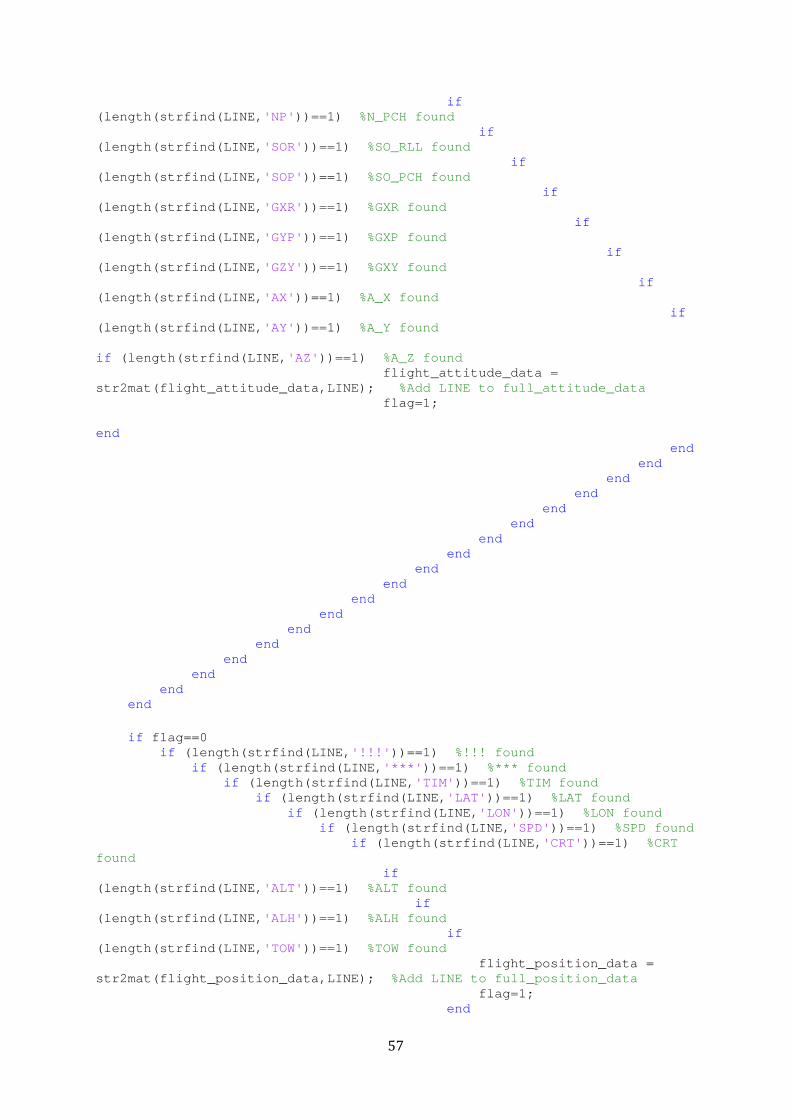
57

if (length(strfind(LINE,'NP'))==1) %N_PCH found if (length(strfind(LINE,'SOR'))==1) %SO_RLL found if (length(strfind(LINE,'SOP'))==1) %SO_PCH found if (length(strfind(LINE,'GXR'))==1) %GXR found if (length(strfind(LINE,'GYP'))==1) %GXP found if (length(strfind(LINE,'GZY'))==1) %GXY found if (length(strfind(LINE,'AX'))==1) %A_X found if (length(strfind(LINE,'AY'))==1) %A_Y found if (length(strfind(LINE,'AZ'))==1) %A_Z found flight_attitude_data = str2mat(flight_attitude_data,LINE); %Add LINE to full_attitude_data flag=1; end end end end end end end end end end end end end end end end end end end if flag==0 if (length(strfind(LINE,'!!!'))==1) %!!! found if (length(strfind(LINE,'***'))==1) %*** found if (length(strfind(LINE,'TIM'))==1) %TIM found if (length(strfind(LINE,'LAT'))==1) %LAT found if (length(strfind(LINE,'LON'))==1) %LON found if (length(strfind(LINE,'SPD'))==1) %SPD found if (length(strfind(LINE,'CRT'))==1) %CRT found if (length(strfind(LINE,'ALT'))==1) %ALT found if (length(strfind(LINE,'ALH'))==1) %ALH found if (length(strfind(LINE,'TOW'))==1) %TOW found flight_position_data = str2mat(flight_position_data,LINE); %Add LINE to full_position_data flag=1; end

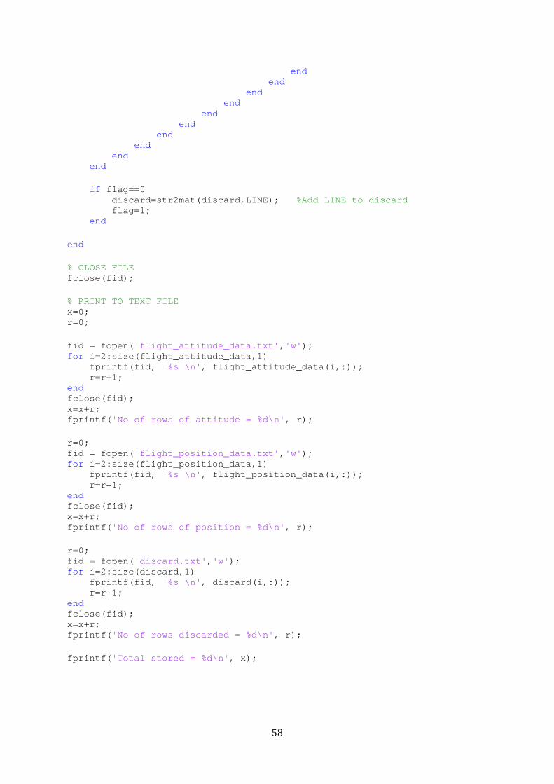
58

end end end end end end end end end end if flag==0 discard=str2mat(discard,LINE); %Add LINE to discard flag=1; end end % CLOSE FILE fclose(fid); % PRINT TO TEXT FILE x=0; r=0; fid = fopen('flight_attitude_data.txt','w'); for i=2:size(flight_attitude_data,1) fprintf(fid, '%s \n', flight_attitude_data(i,:)); r=r+1; end fclose(fid); x=x+r; fprintf('No of rows of attitude = %d\n', r); r=0; fid = fopen('flight_position_data.txt','w'); for i=2:size(flight_position_data,1) fprintf(fid, '%s \n', flight_position_data(i,:)); r=r+1; end fclose(fid); x=x+r; fprintf('No of rows of position = %d\n', r); r=0; fid = fopen('discard.txt','w'); for i=2:size(discard,1) fprintf(fid, '%s \n', discard(i,:)); r=r+1; end fclose(fid); x=x+r; fprintf('No of rows discarded = %d\n', r); fprintf('Total stored = %d\n', x);