Graduate Theses, Dissertations, and Problem Reports

2012

UAV Simulation Environment for Autonomous Flight Control UAV Simulation Environment for Autonomous Flight Control

Algorithms Algorithms

Ondrej Karas West Virginia University

Follow this and additional works at: https://researchrepository.wvu.edu/etd

Recommended Citation Recommended Citation Karas, Ondrej, "UAV Simulation Environment for Autonomous Flight Control Algorithms" (2012). Graduate Theses, Dissertations, and Problem Reports. 487. https://researchrepository.wvu.edu/etd/487

This Thesis is protected by copyright and/or related rights. It has been brought to you by the The Research Repository @ WVU with permission from the rights-holder(s). You are free to use this Thesis in any way that is permitted by the copyright and related rights legislation that applies to your use. For other uses you must obtain permission from the rights-holder(s) directly, unless additional rights are indicated by a Creative Commons license in the record and/ or on the work itself. This Thesis has been accepted for inclusion in WVU Graduate Theses, Dissertations, and Problem Reports collection by an authorized administrator of The Research Repository @ WVU. For more information, please contact researchrepository@mail.wvu.edu.

UAV Simulation Environment for

Autonomous Flight Control Algorithms

Ondřej Karas

Thesis submitted to the

Benjamin M. Statler College of Engineering and Mineral Resources

at West Virginia University

in partial fulfillment of the requirements for the degree of

Master of Science

in

Aerospace Engineering

Dr. Mario Perhinschi, Chair

Dr. Marcello Napolitano

Dr. Peter Gall

Mechanical and Aerospace Engineering Department

Morgantown, West Virginia

2012

Keywords: Simulation Environment; Unmanned Aerial Vehicles;

Flight Control Laws; Path Planning; Abnormal Conditions

Copyright 2012 Ondřej Karas

ABSTRACT

UAV Simulation Environment for Autonomous Flight Control Algorithms

Ondřej Karas

This thesis presents the development of a UAV simulation environment for the design,

analysis, and comparison of autonomous flight control laws. The simulation environment

was developed in MATLAB/Simulink, with custom map generation software and

FlightGear 3-D visualization. Graphical user interface of the simulation environment is

user-friendly and all available options are discussed in detail. Aircraft dynamic models

are presented, with emphasis on newly designed UAV models. Five different aircraft

models are available, with several path planning and trajectory tracking algorithms

implemented. Emphasis is given to simulation of failures and other abnormal conditions,

so that appropriate tools for failure detection, evaluation, and accommodation can be

designed. The development of new path planning methodologies, such as optimized point

of interest or automatic landing algorithms, is introduced. New developments in

trajectory tracking algorithms, including adaptive controllers are discussed. An example

simulation study is presented to investigate obstacle avoidance path planning algorithms,

as well as the performance of trajectory tracking algorithms under both nominal and

failure conditions. The results of this study are discussed with respect to optimum

algorithm choice, as well as the user-friendliness of the UAV simulation environment as

a whole. Finally, possible strategies for future improvements and expansion of the UAV

simulation environment and its components are introduced.

iii

TABLE OF CONTENTS

Chapter Page

I. INTRODUCTION ......................................................................................................1

1.1 Background ........................................................................................................1

1.2 Objectives ..........................................................................................................2

1.3 Thesis Layout .....................................................................................................2

II. GENERAL ARCHITECTURE OF THE SIMULATION ENVIRONMENT ..........4

III. GRAPHICAL USER INTERFACE ........................................................................7

3.1 MATLAB Setup GUIs .......................................................................................8

3.1.1 Number of Vehicles GUI ..........................................................................8

3.1.2 General GUI ..............................................................................................9

3.1.3 Aircraft Specific GUI ..............................................................................10

3.2 Simulink Block Controls..................................................................................11

3.2.1 Algorithm Switching ...............................................................................12

3.2.2 Wind and Turbulence Controls ...............................................................13

3.2.3 Time Acceleration ...................................................................................15

3.2.4 Scopes and Plots .....................................................................................15

3.2.5 Trajectory Save/Load Functions .............................................................16

3.2.6 Simulation Reload Button .......................................................................17

3.2.7 FlightGear and UAV Dashboard Start ....................................................17

3.3 Flight Path Visualization..................................................................................18

3.3.1 FlightGear ...............................................................................................18

3.3.2 UAV Dashboard......................................................................................19

IV. AIRCRAFT DYNAMICS .....................................................................................22

4.1 WVU YF-22.....................................................................................................22

4.2 NASA GTM .....................................................................................................23

4.3 Pioneer UAV ....................................................................................................24

4.3.1 Wind Tunnel Model ................................................................................25

4.3.2 Geometric Analysis Using AVL .............................................................26

4.3.3 Geometric Analysis Using DATCOM ....................................................28

4.3.4 Correction Factor Generation .................................................................28

4.3.5 Simulink Implementation........................................................................31

iv

Chapter Page

4.4 TigerShark UAV ..............................................................................................32

4.4.1 Comparison with Pioneer UAV ..............................................................32

4.4.2 Geometric Analysis Using AVL .............................................................34

4.4.3 Corrected Analysis Using Pioneer Correction Factors ...........................34

4.5 OX UAV ..........................................................................................................36

4.5.1 Geometric Analysis Using AVL .............................................................36

4.5.2 Engine Model ..........................................................................................37

4.5.3 Stall Model ..............................................................................................39

4.5.4 Landing Gear Model ...............................................................................40

V. PATH PLANNING ................................................................................................42

5.1 Obstacle Avoidance Techniques ......................................................................42

5.1.1 Voronoi ...................................................................................................42

5.1.2 Grid .........................................................................................................44

5.1.3 Potential Field .........................................................................................44

5.2 Point of Interest Algorithms.............................................................................45

5.2.1 Traditional Algorithms............................................................................45

5.2.2 Shortest Path Justification .......................................................................46

VI. TRAJECTORY TRACKING ................................................................................51

6.1 Path to Trajectory Conversion .........................................................................51

6.2 Simulink Implementation.................................................................................52

6.2.1 Trajectory Definition ..............................................................................52

6.2.2 Simulation Run Time ..............................................................................52

6.2.3 Simulation Integration Step ....................................................................52

6.3 Trajectory Tracking Algorithms ......................................................................53

6.3.1 Heading PID............................................................................................53

6.3.2 Position PID ............................................................................................53

6.3.3 Outer Loop NLDI ...................................................................................54

6.3.4 Extended NLDI .......................................................................................54

6.3.5 LQR.........................................................................................................55

6.3.6 Adaptive Algorithms ...............................................................................55

6.3.7 Simulink Implementation........................................................................56

6.4 Formation Flight ..............................................................................................57

v

Chapter Page

VII. ABNORMAL CONDITIONS ..............................................................................59

7.1 Failures .............................................................................................................59

7.1.1 Structural .................................................................................................59

7.1.2 Controls ...................................................................................................60

7.1.3 Sensors ....................................................................................................60

7.2 Mission Re-plan ...............................................................................................60

7.2.1 Tactical Re-plan ......................................................................................60

7.2.2 Diversion to Nearest Runway .................................................................61

VIII. SIMULATION RESULTS .................................................................................64

8.1 Obstacle Avoidance Path Planner Comparison Study .....................................64

8.2 Controller Comparison Study ..........................................................................68

8.2.1 Tracking Performance .............................................................................68

8.2.2 Failures ....................................................................................................73

IX. CONCLUSIONS ...................................................................................................76

REFERENCES ............................................................................................................78

APPENDIX A: UAV SIMULATION ENVIRONMENT USER GUIDE ..................82

APPENDIX B: MATLAB/SIMULINK IMPLEMENTATION ..................................84

APPENDIX C: AIRCRAFT MODEL DESIGN CALCULATIONS ..........................94

vi

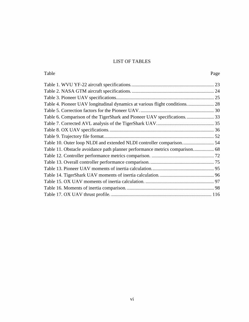
LIST OF TABLES

Table Page Page

Table 1. WVU YF-22 aircraft specifications. ................................................................... 23

Table 2. NASA GTM aircraft specifications. ................................................................... 24

Table 3. Pioneer UAV specifications................................................................................ 25

Table 4. Pioneer UAV longitudinal dynamics at various flight conditions. ..................... 28

Table 5. Correction factors for the Pioneer UAV. ............................................................ 30

Table 6. Comparison of the TigerShark and Pioneer UAV specifications. ...................... 33

Table 7. Corrected AVL analysis of the TigerShark UAV. .............................................. 35

Table 8. OX UAV specifications. ..................................................................................... 36

Table 9. Trajectory file format. ......................................................................................... 52

Table 10. Outer loop NLDI and extended NLDI controller comparison. ......................... 54

Table 11. Obstacle avoidance path planner performance metrics comparison. ................ 68

Table 12. Controller performance metrics comparison. ................................................... 72

Table 13. Overall controller performance comparison. .................................................... 75

Table 13. Pioneer UAV moments of inertia calculation. .................................................. 95

Table 14. TigerShark UAV moments of inertia calculation. ............................................ 96

Table 15. OX UAV moments of inertia calculation. ........................................................ 97

Table 16. Moments of inertia comparison. ....................................................................... 98

Table 17. OX UAV thrust profile. .................................................................................. 116

vii

LIST OF FIGURES

Figure Page

Figure 1. General architecture of the UAV simulation environment. ................................. 5

Figure 2. Path planning, trajectory generation and tracking data transfer. ......................... 6

Figure 3. User interface with the UAV simulation environment. ....................................... 8

Figure 4. Number of Vehicles GUI..................................................................................... 9

Figure 5. General GUI. ..................................................................................................... 10

Figure 6. Aircraft specific GUI for the WVU F-22. ......................................................... 11

Figure 7. Simulink block controls within the WVU F-22 Simulink model. ..................... 12

Figure 8. Wind & Turbulence Simulink block organization and contents. ...................... 14

Figure 9. Scopes selection menu for the WVU F-22 model. ............................................ 15

Figure 10. Plots selection menu for the WVU F-22 model. ............................................. 16

Figure 11. Pioneer UAV model in FlightGear. ................................................................. 18

Figure 12. HUD interface in FlightGear. .......................................................................... 19

Figure 13. San Francisco Bay area map for the UAV Dashboard. ................................... 20

Figure 14. Typical mission plan on the UAV Dashboard. ................................................ 21

Figure 15. 3D visual model of the Pioneer UAV.............................................................. 25

Figure 16. AVL visualization of the Pioneer UAV model. .............................................. 27

Figure 17. Pioneer flight dynamics block structure. ......................................................... 31

Figure 18. Pioneer flight dynamics Simulink block. ........................................................ 32

Figure 19. Geometry comparison of the TigerShark and Pioneer UAVs. ........................ 33

Figure 20. AVL visualization of the TigerShark UAV model. ......................................... 34

Figure 21. Maximum rate of climb as a function of velocity simulation experiment. ..... 38

Figure 22. Maximum rate of climb comparison with flight test data. .............................. 39

Figure 23. Lift and drag curves for the NACA 63-415 profile20

. ..................................... 40

Figure 24. Landing gear model structure. ......................................................................... 41

Figure 25. A Voronoi Diagram24

. ..................................................................................... 43

Figure 26. Grid algorithm visualization. ........................................................................... 44

Figure 27. Potential field showing force vectors26

............................................................ 45

Figure 28. Shortest flyable path geometry. ....................................................................... 47

Figure 29. Advance turn ratio as a function of segment lengths for θ = 90°. ................... 48

Figure 30. Turn generation flowchart. .............................................................................. 49

Figure 31. Point of interest algorithm trajectory generation sequence. ............................ 50

Figure 32. Position PID controller schematic. .................................................................. 54

viii

Figure Page

Figure 33. Simulink implementation of trajectory tracking algorithms. .......................... 56

Figure 34. Formation flight schematic. ............................................................................. 57

Figure 35. YF-22s flying in formation. ............................................................................. 58

Figure 36. Automatic approach to landing geometry. ...................................................... 62

Figure 37. Voronoi diagram featuring obstacle shapes and selected path. ....................... 65

Figure 38. Grid algorithm plot showing selected path and obstacles. .............................. 66

Figure 39. POI v2 path visualization through UAV Dashboard. ...................................... 67

Figure 40. Controller comparison trajectory 2-D visualization. ....................................... 69

Figure 41. Throttle control comparison. ........................................................................... 71

Figure 42. Cost function in terms of required performance threshold. ............................. 74

Figure 43. Algorithm selector block within the WVU F-22 Simulink model. ................. 85

Figure 44. Manual flight block within the WVU F-22 Simulink model. ......................... 86

Figure 45. Follow leader block within the WVU F-22 Simulink model. ......................... 86

Figure 46. Aerodynamic forces computation within the Pioneer Simulink model. .......... 90

Figure 47. Data manager block within the WVU F-22 Simulink model. ......................... 91

Figure 48. FlightGear data transfer block within the WVU F-22 Simulink model. ......... 92

Figure 49. Dashboard data transfer block within the WVU F-22 Simulink model. ......... 93

Figure 50. OX UAV thrust profile graph. ....................................................................... 117

1

CHAPTER I

INTRODUCTION

1.1 Background

The use of unmanned aerial vehicles (UAVs) for missions ranging from intelligence and

reconnaissance to electronic warfare and even payload delivery is becoming increasingly

popular1. Flight duration on some missions can easily exceed 24 hours, creating large

demands on ground staff who plan the missions, monitor the vehicles' progress and

recover the UAVs from problematic or dangerous situations. These tasks can be

monotonous, repetitive, and tiring for human operators2. They can also become

overwhelming in situations when unexpected threats appear in the arena or if the vehicle

is damaged. Humans are best at strategic planning and even resolving abnormal situations

provided they have sufficient time to react. However, it is becoming increasingly

important for UAVs to be able to perform simple and repetitive tasks autonomously.

Furthermore, they should be able to correctly react in the first moments of a developing

emergency and facilitate the tasks of the human operator. In a hostile electronic warfare

environment, the communication links between the ground station/satellite and the UAV

may be severed. The ground staff can only receive feedback from the vehicle by visual

means, making it more difficult for the human brain to process the information and react

appropriately. For example, recovery from unusual attitudes can become extremely

difficult when looking at a fuzzy screen image.

However, the challenges of UAV operations in complex hostile environments are not

limited to avoiding threats and recovering the vehicle from precarious situations. With

limited resources, it is also important that each UAV mission can accomplish as many

tasks as possible3. Tactical flight planning can become an intricate task, especially when

multiple UAVs are involved. To accomplish this on a time crunch is extremely difficult

and requires vast human resources, which may not always be available. The best answer

to these concerns is full automation of UAV missions at all levels, starting with tactical

planning, through aircraft control under nominal conditions, until provisions for

autonomous flight under abnormal conditions.

2

Typically, UAV simulation tools have been focused on a single aspect of UAV operation,

such as vehicle dynamics and control, flight planning or cooperative control. Generally, a

simulation environment has been tailored to a single UAV type and research has been

done on flight control system design at nominal conditions. The efforts for the

development of highly flexible, fault-tolerant controllers have been limited due to the fact

that this research requires testing in a large variety of conditions.

Some examples of today's UAV simulation tools are Simdrone4, Chungnam National

University simulation environment for multiple UAVs5, as well as commercial

simulators, such as FlightGear6 or X-Plane

7. Simdrone is focused on operator training and

features exceptionally detailed graphical environment; however, it is limited to

conventional flight control systems (weControl autopilot). Chungham University

simulator allows simulation of multiple UAVs; however it uses the default Simulink

Aerosonde UAV model to simulate the aircraft dynamics. FlightGear and X-Plane are

successful multi-purpose commercial simulators, which feature detailed graphics and

thousands of aircraft models, but they have minimal provisions for flight control system

design (only allowing PID control).

There is no publicly available software, specifically adapted to UAV trajectory planning

algorithm and flight control system design that would feature several different aircraft

models, simulate flight dynamics in such detail, and consider abnormal conditions, such

as aircraft sub-system failures.

1.2 Objectives

The main objective of this thesis is to present a simulation environment framework for

the development of autonomous flight control laws, which would address the need for

full automation of flight planning, execution of complex UAV missions, and real-time

adaptation to actual normal and abnormal conditions. Not only does this thesis present the

comprehensive simulation tools that have been created for the development,

implementation, evaluation, and testing of autonomous flight control algorithms; but it

also includes a short introduction to the techniques that can be used to develop more

capable, flexible, and, at the same time, robust control laws. A special emphasis is given

to provisions for adaptive flight control laws, which allow for failure detection,

identification, evaluation, and accommodation. The West Virginia University (WVU)

UAV simulation environment is designed to cater for easy evaluation and comparison of

different flight control schemes. Finally, the actual implementation of the flight control

laws developed in the simulation environment is facilitated by giving consideration to

real world environmental conditions, such as wind or turbulence. All of the above is done

with user-friendliness in mind.

3

1.3 Thesis Layout

The thesis is organized as follows:

Chapter II describes the general architecture of the simulation environment, giving a

basic overview of its organization and the software, in which it is implemented.

Chapter III describes in detail the graphical user interface (GUI) with the simulation

environment and its operation. This chapter also refers to an abbreviated "User Guide"

included in Appendix A. Chapter IV describes the five aircraft models currently

implemented in the UAV simulation environment. Three of these models have been

newly designed for this environment and the process of obtaining a flight dynamics

model from limited publicly available information is presented in this chapter. Chapter V

focuses on the path planning techniques and algorithms currently present in the

simulation environment, describing a shortest path point of interest algorithm in detail.

Chapter VI discusses how trajectories are handled within the UAV simulation

environment and presents the steps taken to obtain a flyable trajectory from a geometric

path. It also gives a brief overview of the trajectory tracking algorithms already available

within the simulation environment. Chapter VII describes the various abnormal

conditions (aircraft failures and challenging environmental factors), which can be

simulated. It also presents the on board intelligence developed to mitigate the effects of

these adverse conditions. The results of example comparison studies among the available

path planners and controllers are presented in Chapter VIII. Finally, Chapter IX draws

conclusions from the challenges encountered while carrying out these comparison studies

and discusses potential for future improvements.

4

CHAPTER II

GENERAL ARCHITECTURE

The WVU UAV simulation environment is developed in MATLAB and Simulink, which

allows quick updates and implementation of new algorithms. The simulation environment

is interfaced with the FlightGear6 open-source simulation package for visualization. It

further interfaces with a customized map generation and visual feedback environment

called UAV Dashboard8, which is created in C#. A highly modular architecture has been

adopted to allow easy upgrade or addition of individual components. Simulation can be

run in real time or accelerated time. This section describes the major components of the

simulation environment, explains their functions and lists the data that is passed between

them. Figure 1 shows a simplified graphical representation of the relationships between

the various modules within the UAV simulation environment.

The UAV simulation environment is centered on several aircraft aerodynamic models.

Each aircraft model is integrated within its dedicated Simulink block. Non-linear vehicle

equations of motion are at the heart of each model. This core is connected to appropriate

aircraft-specific equations and look-up tables, which capture the dynamics of each UAV

type. Currently, five different UAVs can be simulated.

The Simulink block of each aircraft accepts generalized control commands (elevator,

aileron, rudder, and throttle signals) as its inputs. It also receives inputs from a model of

the outside environment, such as steady wind, gusts, or turbulence. A set of 41 state

variables is updated at each integration step. This set is then passed to visualization

modules, such as FlightGear and UAV Dashboard as well as stored for later analysis by

the user. Finally, a sensor feedback model is implemented, which processes the state

variables and transforms them into realistic simulated sensor readout. This signal is then

fed back to the trajectory tracking algorithms, which are used to control the flight path of

the vehicle.

5

Figure 1. General architecture of the UAV simulation environment.

The primary objective of the UAV simulation environment is to facilitate the design,

testing, evaluation, comparison and implementation of different trajectory planning and

tracking algorithms for UAV autonomous flight. Therefore, the various path planning,

trajectory generation and tracking algorithms are designed to be easily upgradable and

replaceable. A new path planner can be easily added, replaced or upgraded without

affecting the rest of the simulation environment or the other algorithms present.

Similarly, a trajectory tracking algorithm (controller) can be replaced while keeping all

other components in place. This architecture allows the user to compare and contrast

various algorithms.

Path planning and trajectory generation algorithm are universal for all simulated aircraft

with minor differences, such as aircraft flight envelope and maneuverability properties.

Therefore, replacing the m-files associated with any of these algorithms will affect all

UAVs in the simulation environment. On the other hand, trajectory tracking algorithms

have numerous aircraft dynamical characteristics embedded in them by design. These

algorithms are implemented in Simulink as independent blocks. Replacing these

controller blocks will only replace the trajectory tracking algorithms for a specific UAV.

6

There are two types of trajectory planning and generation modules: split and integrated.

In the split modules, the desired path to be flown is geometrically computed. It is then

converted into a trajectory and fed to the trajectory tracking modules (controllers) at each

time step. In the integrated modules, a trajectory is generated directly via a MATLAB

code, which decides where to place the next trajectory point at each time step. Finally, a

prerecorded trajectory can be flown instead of a planned trajectory. Prerecorded

trajectories are stored in a common format: A vertically oriented array, where the lines

contain position and velocity vectors in Cartesian coordinates at each time step.

Path planning and trajectory generation algorithms obtain the user inputs, such as initial

aircraft position, target and waypoint location(s), threat location(s) and properties, from

the UAV Dashboard software via a set of text files. Conversely, these algorithms pass the

desired aircraft track back to the UAV Dashboard for visualization via a User Datagram

Protocol (UDP). Trajectory generators further send a commanded position in Cartesian

coordinates as well as a commanded velocity vector in Cartesian coordinates to the

trajectory tracking algorithms. This ensures that data is passed in a standard format,

which in turn allows a modular organization of the algorithms. Finally, the trajectory

tracking algorithms send their elevator, aileron, rudder, and throttle commands in a

standard format to the aircraft model. Figure 2 presents a schematic of the data transfer

signals used to pass data among the various algorithms.

Each UAV model has provisions made for manual flight control. This is essential for

aircraft model validation and dynamic analysis. For manual flight, the path planners and

trajectory generators are deactivated and, instead of using a controller block, the flight

control commands are provided by the joystick. The joystick signal is calibrated so that

the control authority (range of control surface deflections) that be achieved in manual

flight is same as the control authority of the trajectory trackers.

Figure 2. Path planning, trajectory generation and tracking data transfer.

7

CHAPTER III

GRAPHICAL USER INTERFACE

A simple and user-friendly interface with the simulation environment enables the end

user to set up the simulation, adjust its parameters, and obtain the required data quickly

and hassle free. There are several requirements for the GUI to be efficient.

First of all, all simulation features, options and parameters have to be available in the set-

up interface. Secondly, the time required to start a simulation should be minimized, even

for an inexperienced user. It is likely that a set of similar simulations would be run during

a typical experiment, adjusting one or two parameters between each simulation run. This

means that, once a simulation has been completed, it should be easy for the user to run a

similar, yet altered simulation. Finally, the user should be presented all the data that

might interest them in an intuitive manner, making it easy to spot the general

characteristics of the simulation and compare the results of several simulations at a

glance.

The UAV simulation environment therefore offers 2-D as well as 3-D flight path

visualization tools, in addition to plots and scopes for all relevant parameters. The same

data is presented in a variety of different ways, with several levels of intuitiveness and

precision. This allows the user to immediately determine the basic results of a simulation,

such as whether the aircraft is following a desired trajectory. At the same time, detailed

comparison between similar sets of data collected throughout several simulations is

available using MATLAB plots, as well as numerical data stored automatically at the end

of every simulation. Figure 3 shows the user interface with the UAV simulation

environment.

8

Figure 3. User interface with the UAV simulation environment.

3.1 MATLAB Setup GUIs

The initial sequence of GUIs used to start up the simulation and initialize all required

parameters is implemented in MATLAB. The simulation is started through the MATLAB

command window by entering the root (main) simulation folder and typing the command

"WVUUAV". This script clears the workspace, closes any other simulations that might

be running, adds required folders to the MATLAB path and opens the "Number of

Vehicles" GUI, the first step of the simulation setup.

3.1.1 Number of Vehicles GUI

The first GUI in the sequence allows the user to choose whether the flight of a single

UAV would be simulated or whether there would be multiple vehicles. At present, only

one UAV can be simulated at a time, with the exception of formation flight. However,

this GUI gives a provision for future expansion of the simulation environment, which will

allow the testing of algorithms for cooperative UAV operations. Figure 4 shows the

appearance of the "Number of Vehicles" GUI.

9

Figure 4. Number of Vehicles GUI.

Clicking the "LAUNCH" button sends the user to the "General" GUI, which enables

them to select the parameters for each simulated vehicle. This GUI either runs once (if a

single vehicle is simulated) or several times (when the multiple vehicles option is

chosen).

3.1.2 General GUI

The general GUI is where the user can select the main options of the simulation scenario.

The GUI visualization is shown in Figure 5. First of all, the type of aircraft to be

simulated is chosen. At present, five different aircraft are modeled (described in more

detail in the Aircraft Dynamics section of this thesis). Each UAV has its own MATLAB

dynamic aircraft model as well as a 3-D visualization implemented in FlightGear.

Secondly, a map is selected to be used for the visual environment within FlightGear and

UAV Dashboard map interface. The only map available at the moment is the San

Francisco Bay Area shown in Figure 13. Next, artificial intelligence to be used to guide

and control the simulated flight is selected.

A modular architecture consisting of several trajectory planning algorithms as well as

trajectory tracking algorithms has been implemented. Any trajectory planner can be

selected in combination with any controller. Both conventional and adaptive versions of

each controller (except for LQR) are available and can be accessed using a switch in the

user interface. Once all the desired options have been selected, the "LOAD" button saves

the selection in a file that would be used to start up the simulation. It also enables the

"VISUALS" and "LAUNCH" buttons. "VISUALS" runs a script, which initializes both

FlightGear and Dashboard interfaces for the selected aircraft. "LAUNCH" button sends

the user to an aircraft specific GUI for the selected UAV.

10

Figure 5. General GUI.

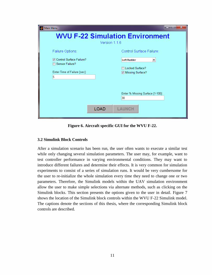
3.1.3 Aircraft Specific GUI

The aircraft specific GUI allows selection of parameters for abnormal conditions that can

affect the simulated aircraft. It also lets the user select the configuration of the simulated

aircraft, where multiple configurations are available. An aircraft specific GUI for the

WVU F-22 UAV is shown in Figure 6. This particular GUI lets the user select from a

variety of control surface failures, as well as sensor failures that are described in more

detail in the Aircraft Dynamics section. As in the general GUI, once the user has selected

the desired values for all parameters, the "LOAD" button is pressed. This saves the

desired parameters into a file and enables the "LAUNCH" button. Upon pressing this

button, the Simulink model of the selected UAV is initialized.

11

Figure 6. Aircraft specific GUI for the WVU F-22.

3.2 Simulink Block Controls

After a simulation scenario has been run, the user often wants to execute a similar test

while only changing several simulation parameters. The user may, for example, want to

test controller performance in varying environmental conditions. They may want to

introduce different failures and determine their effects. It is very common for simulation

experiments to consist of a series of simulation runs. It would be very cumbersome for

the user to re-initialize the whole simulation every time they need to change one or two

parameters. Therefore, the Simulink models within the UAV simulation environment

allow the user to make simple selections via alternate methods, such as clicking on the

Simulink blocks. This section presents the options given to the user in detail. Figure 7

shows the location of the Simulink block controls within the WVU F-22 Simulink model.

The captions denote the sections of this thesis, where the corresponding Simulink block

controls are described.

12

Figure 7. Simulink block controls within the WVU F-22 Simulink model.

3.2.1 Algorithm Switching

Switching between different path planning and trajectory tracking algorithms is

anticipated to be one of the most common tasks that a user has to perform repeatedly in

order to run a series of test cases. Therefore, the UAV simulation environment has been

designed to make this task extremely simple. There are two ways that can be used to

switch to a different algorithm:

First, when the simulation is not running, clicking on a path planning or trajectory

tracking algorithm Simulink block will activate the corresponding algorithm. A callback

function is run, which first ensures that the user is in the correct MATLAB directory, sets

the appropriate value to the "TrTrackAlg" or "TrPlanAlg" variable, sets correct values to

corresponding variables (such as engaging a default controller when a path planning

algorithm is being activated). Finally the MATLAB script "SetColors.m" is run to reset

the colors of the Simulink blocks in the interface to the new settings. The script from the

WVU F-22 Simulink model can be seen in Appendix B.

Secondly, the algorithms may be switched while the simulation is running, using

appropriate joystick buttons. This can be useful, for example, when the user desires to

manually deviate from the planned trajectory to simulate a temporary equipment failure.

The user may thus disengage a trajectory tracking algorithm, perform a manual

maneuver, and then reengage the controller. Another case may be when the user decides

to re-plan the trajectory at a given moment by engaging a different trajectory generator.

The switching procedure is described in detail in the "User's Guide to the UAV

13

simulation environment" in Appendix A. It is only available when an appropriate joystick

(with at least 6 buttons) is used. Appendix B shows the complex Simulink block, which is

used for the algorithm switching, and describes its operation. Figure 33 in section 6.3.7

shows the implementation of the trajectory tracking algorithms within the UAV

simulation environment, as seen from the user's perspective.

3.2.2 Wind and Turbulence Controls

Similarly, the level of turbulence can be set by clicking on the "Wind & Turbulence"

Simulink block within the simulation environment. A callback function is run, which

switches to the next turbulence level, and also adjusts the block color and label. Five

different turbulence severities are available: 0, 3, 10, 20, and 50. The numbers describe

the square of Dryden model standard deviation in m/s. Zero is the default value and it

corresponds to no wind or steady wind.

The "Wind & Turbulence" Simulink block also contains a steady wind model, which gets

added to the turbulence effects. The wind speed and direction are set through constants

located in the highest level of the UAV Simulink model; they are sent to the "Wind &

Turbulence" block by the use of labels. Figure 8 shows the organization of the "Wind &

Turbulence" block and the contents of each part.

14

Figure 8. Wind & Turbulence Simulink block organization and contents.

15

3.2.3 Time Acceleration

The simulation runs, which a user may wish to execute in the UAV simulation

environment, can range from a single maneuver to a long and complex mission scenario.

Depending on the tasks of each simulation run, the user may elect to follow the

simulation in real time or accelerate it and later analyze its results. Therefore, the

simulation environment provides two options for time acceleration: real time (no

acceleration), and accelerated time (as fast as the computer processing power allows).

The selection is done by clicking on a Simulink block, which contains an Enabled

Subsystem. A callback function is run, which either enables or disables the subsystem. A

Simulation Pace block is embedded in the Enabled Subsystem. By default, real time is

enabled upon initialization.

3.2.4 Scopes and Plots

Scopes can be used to visualize certain parameters and variations thereof in real time.

They may also be analyzed off-line, following a simulation run. 22 scopes are available

to visualize the following parameters: airspeed, altitude, angle of attack together with

sideslip angle, Euler angles and angular rates, throttle and stick inputs, flight control

surface deflections, and controller errors. Figure 9 shows the scope selection menu

designed for the WVU F-22 model. The menu is implemented as a MATLAB GUI.

Checking a box within this menu will display the corresponding plot. Un-checking a box

will hide the plot. Note that the scopes provided through the high-level simulation

interface are not the only ones available. There are also scopes embedded in critical

signals within the trajectory tracking algorithms, which allow analysis of specific data.

Figure 9. Scopes selection menu for the WVU F-22 model.

16

MATLAB plots are a cleaner and more visually appealing alternative for the presentation

of prerecorded simulation results. Plots are available for the same key variables as

scopes. Furthermore, the desired as well as actual trajectories of the aircraft can be

visualized using plots in both 2-D and 3-D. Figure 10 shows the plot selection menu

implemented in Simulink.

Figure 10. Plots selection menu for the WVU F-22 model.

The entire set of 41 state variables, 4 control variables and 6 tracking errors is also saved

in respective m-files, which allows for later analysis. Figure 47 in Appendix B shows the

Simulink implementation of the "Data Manager" block, which supports scopes, plots, as

well as data storage.

3.2.5 Trajectory Save/Load Functions

In certain occasions it is beneficial to manually "fly" a specific trajectory and save it for

subsequent evaluation of trajectory tracking algorithms. Therefore, an option to save the

trajectory that has been flown since the start of the simulation is provided to the user.

Clicking on the appropriate box, as seen in Figure 7, will run a script that stores the

Cartesian coordinates of each time step, as well as corresponding velocity components in

Cartesian coordinates, in a "Trajectory" file. The user can choose a name of the file.

Upon typing the name, a suffix "_X" is added to the name, where "X" is the number of

seconds that the trajectory would take to run. This has proven to be helpful for later

reference and to distinguish between trajectories with same or similar name.

17

In order to load both pre-recorded and computer pre-generated trajectories from the hard

drive, an appropriate Simulink block is included. Clicking this block runs a script, which

opens a file browser by default in the "StoredPaths" directory. This directory contains all

previously saved trajectories in a structure format. Selecting a trajectory will load the

contents of the corresponding structure into the workspace and, if manual flight had

previously been selected, the default trajectory tracking algorithm will automatically

engage. If the user desires to engage a different controller, they may do so at this stage.

3.2.6 Simulation Reload Button

Simulation reload button erases the workspace and returns the user to the aircraft-specific

GUI stage. The reason for this rationale is that if the user wishes to drastically change the

simulation scenario, such as by selecting a different aircraft, they may do so by exiting

the simulation and starting again. However, in a more common scenario, the user may

wish to change the failures imposed on the aircraft. This can only be done through the

aircraft specific GUI. Hence, the user may use the reload button to select different failure

conditions. Furthermore, the reload button ensures that any variables, which may have

been accidentally modified through the MATLAB command line or third party scripts,

will be restored to default values. It is advisable to reload the simulation upon running

any complicated data analysis code that is suspected to use same variable names as the

UAV simulation environment. Only one variable is essential for the reload button to

work: "currentdir", which stores information about the current directory path. If this

variable has been erased (this may happen by inadvertent use of the "clear" command)

the simulation has to be completely closed and restarted using the "WVUUAV"

command.

3.2.7 FlightGear and UAV Dashboard Start

As mentioned above, both FlightGear and the UAV Dashboard may be started using the

"VISUALS" button in the general GUI; however, the user may also elect to only start one

of these tools. Similarly, they may decide to start a visualization tool at a later stage of

the simulation. To facilitate this process, convenient FlightGear and UAV Dashboard

start buttons are incorporated within the aircraft Simulink models. Clicking on these

blocks runs MATLAB scripts, which subsequently start the corresponding visualization

tool. The blocks themselves contain the required interface tools, which select and process

data to be transferred to the FlightGear and UAV Dashboard software.

18

3.3 Flight Path Visualization

In order to be able to effectively use the UAV simulation environment, the user requires

instant intuitive feedback on the basic flight path characteristics of the simulated vehicles.

Flight path visualization tools are provided to give the user basic high-level qualitative

information on the simulation results, without the need to delve into detailed quantitative

analysis using scopes or plots.

3.3.1 FlightGear

The open-source simulation software package FlightGear is used to visualize the 3-D

motion of the UAV in a high fidelity environment. FlightGear receives input directly

from the aircraft model state variables (positions and velocities) to produce an accurate

image of the moving aircraft. However, to simulate inaccuracies in sensor readings, the

signals passed to simulated ground station instruments (or HUD) are processed through a

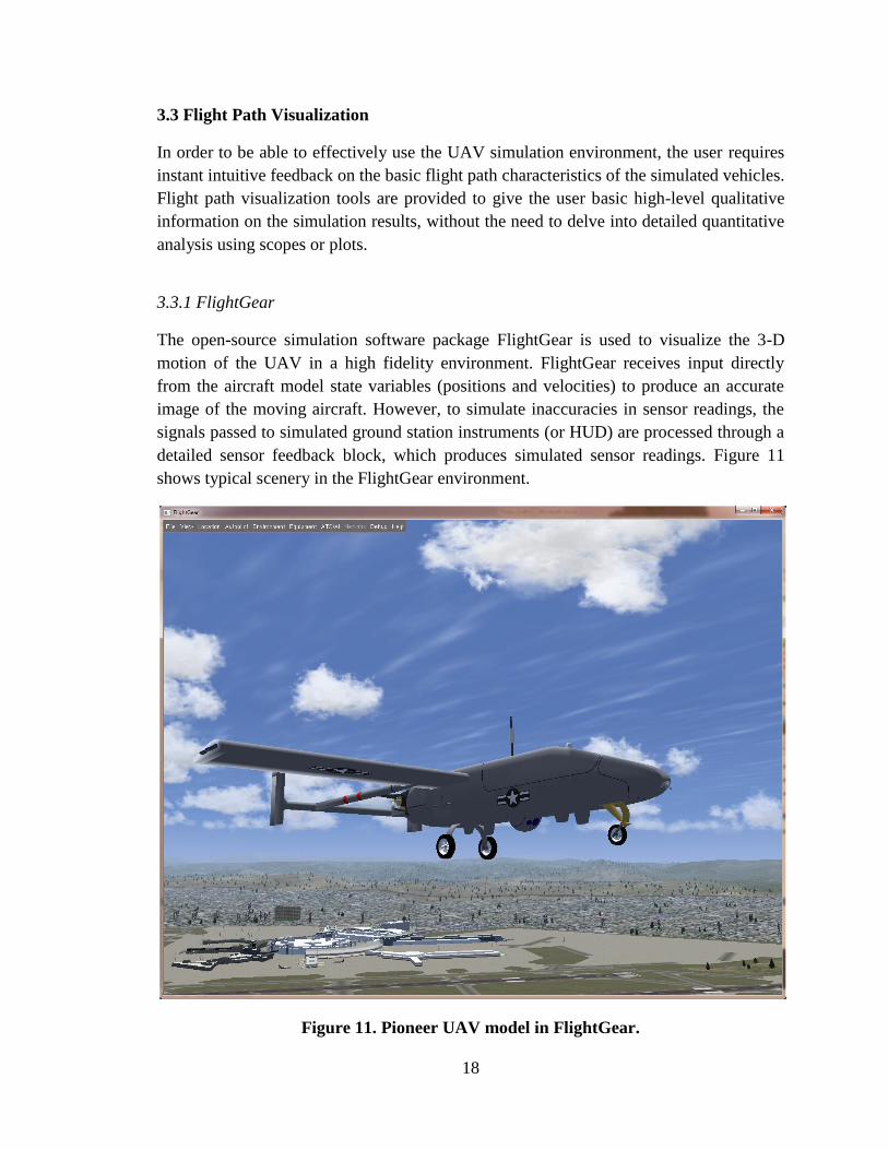
detailed sensor feedback block, which produces simulated sensor readings. Figure 11

shows typical scenery in the FlightGear environment.

Figure 11. Pioneer UAV model in FlightGear.

19

A simple head up display (HUD) interface is generally used to instantly visualize key

parameters. As seen in Figure 12, the HUD permits to quickly determine the aircraft

attitude (pitch, bank angle, and heading), airspeed, altitude, control inputs, and side slip

angle. FlightGear also clearly shows the position of the aircraft, with reference to the

terrain and objects on the ground, such as buildings or runways.

Figure 12. HUD interface in FlightGear.

3.3.2 UAV Dashboard

The UAV Dashboard is custom map generation and visualization software created by

Brenton Wilburn8, which constitutes a significant portion of the graphical user interface

with the UAV simulation environment. The UAV Dashboard has two functions:

First, it is used to generate a strategic mission plan for the simulated UAVs. This includes

a map of targets, which the aircraft should visit, the locations and properties of threat

zones, starting positions of the UAVs and, finally, available landing zones. Threat zones

have “risk intensity” between 0 and 2 assigned to them. A threat zone with risk intensity

20

of 2 means a certain destruction of the vehicle upon entering. While the map is generated,

all information is stored in the form of text files. These text files are subsequently loaded

by the path planners.

The second function of the UAV Dashboard is 2-D visualization of the position and

orientation of the vehicles, with respect to the mission objectives and threat zones. The

desired tracks for the vehicles, as well as their actual tracks, are shown. This allows a

quick evaluation of the performance of the controllers, as well as high-level trajectory

planning analysis.

Various custom-designed maps can be included within the UAV Dashboard to fit a

particular task. Figure 13 shows an example map of the San Francisco Bay area obtained

from Google maps. This area contains several airports, mountainous terrain, populated

areas, as well as water bodies, representing a very diverse environment.

For each simulation scenario, custom threat zones can be positioned anywhere in the

map. These zones can represent surface-to-air missile (SAM) sites and ranges of

operation, anti-aircraft artillery (AAA), or radar facilities. Exposure to any of these

threats increases the probability that the UAV could be destroyed during the mission. It is

therefore the job of the path planning and trajectory generation algorithms to balance

exposure to these threats with the mission objectives.

Figure 13. San Francisco Bay area map for the UAV Dashboard.

21

Typically, high-risk threat zones would be completely avoided unless critical mission

objectives lie within these zones. The UAV Dashboard interface provides the user with

an image similar to that shown in Figure 14, where they can easily determine the route

planned by the selected algorithm, the path actually flown by the aircraft and the position

of both in reference to objects on the map, as well as threat zones. The higher the risk

intensity of a threat zone, the more intense red color is used.

Threat zones may overlap, such as in the case of several AAA sites placed around a

common radar site. In this case, AAA without radar can still destroy the aircraft; however

its precision is much lower than if the UAV also passes through the radar threat zone.

The software includes provisions for 3-D threat zones, which will more accurately

simulate the complex threat environment present in an actual battlefield. For example, the

aircraft may be perfectly safe from a radar site, which is geographically close, but lies

behind a mountain.

Figure 14. Typical mission plan on the UAV Dashboard.

22

CHAPTER IV

AIRCRAFT DYNAMICS

The heart of any aircraft simulation software is the aircraft aerodynamics model. In case

of the UAV simulation environment, there are currently five aircraft models

implemented: WVU YF-229, NASA GTM

10, Pioneer

11, TigerShark

12, and OX

13. Each of

these aircraft has very different dynamical characteristics, adding to the challenge of

developing new flight control algorithms. This chapter presents the available aircraft

aerodynamic models in detail.

4.1 WVU YF-22

The WVU research YF-22 UAV is based on the prototype of the Lockheed/Boeing F-22

fighter aircraft designed for the U.S. Air Force. The WVU research aircraft is scaled

down to approximately 15% of the actual YF-22 size. Table 6 shows the basic

characteristics of this research aircraft. The WVU Y-22 UAV has been specifically

designed for the testing of various flight control algorithms, flight under failure

conditions and their accommodation. Hence the tasks of the aircraft itself are very similar

to that of those of the UAV simulation environment.

A detailed dynamic aircraft model for the YF-22 was developed by WVU researchers14

,

in order to develop flight control algorithms for this UAV and test them prior to

uploading the code on the actual aircraft. Equations of motion block from the Flight

Dynamics and Control MATLAB toolbox15

was used to solve the equations of motion.

The basic characteristics and contents of the aircraft dynamics block for this aircraft were

left unchanged upon implementing the model within the UAV simulation environment.

However, certain unused signals, which were already obsolete in the original model, have

been eliminated. This includes the elimination of flap position signals from the state

variable vector. Furthermore, the numerous MATLAB scripts present in the original

folder were processed, unused scripts were eliminated, and the rest was unified into two

23

files: "F22Start.m" and "AircraftModel.m". The model was then used as a basis for future

aircraft dynamics model development: for the Pioneer, TigerShark, and OX UAVs.

Table 1. WVU YF-22 aircraft specifications.

Parameter Value

Wingspan 6' 6''

Length 10' (with probe)

Height 2'

Wing Area 14.7 ft2

Takeoff Weight 50 lbs

Payload 10-12 lbs

Fuel Capacity 7 lbs

Endurance 12 minutes

Takeoff Speed 52 KIAS

Cruise Speed 78 KIAS

Engine Thrust 28 lbs

The WVU YF-22 is powered by miniature jet engines, and its limited fuel capacity only

allows for approximately 12 minutes of flight. This is in strong contrast with the typical

mid-size military UAVs, whose endurance is in the order of multiple hours. Yet, short

term tactical scenarios and advanced trajectory tracking algorithm testing can be easily

performed using this vehicle. The aircraft was used for formation flight algorithm

testing16

, as well as automated failure identification and evaluation (FDIE)9.

Extensive flight testing was carried out to determine the characteristics of the aircraft

under failure conditions (locked flight control surfaces). This allowed the creation of a

sophisticated failure model further described in section 7.2.

4.2 NASA GTM

NASA's Langley Research Center in Hampton, VA has developed a UAV called the

"Generic Transport Model" or GTM10

. This aircraft is a 5.5% scaled down model of the

Boeing 757, used for research purposes such as post-stall characteristics or flight control

algorithm testing. The GTM, also known as AirSTAR, is turbine powered, giving it a

dash speed in excess of 200 miles per hour. Basic specifications of the NASA GTM are

shown in Table 2.

The Simulink model of the NASA GTM is highly popular amongst flight dynamics

researchers. The fact that the model allows simulation of numerous failures, as well as the

24

high fidelity of its dynamics backed by flight test data, make it an acclaimed tool for the

exploration of new techniques in flight dynamics analysis and automatic flight control

design.

The design of the GTM flight dynamics model differs substantially from all other aircraft

models within the UAV simulation environment. Its dynamics are highly non-linear and

use numerous lookup tables instead of stability and control derivatives. For this reason,

the GTM model has not been upgraded to the same standards of functionality as the

remaining aircraft. For example, landing gear or detailed stall models have not been

included. The controllers can only be preselected through the general GUI or selected by

clicking on the respective controller block before the simulation is started. Algorithm

switching using joystick buttons while the simulation is running is not available for the

GTM.

Table 2. NASA GTM aircraft specifications.

Parameter Value

Wingspan 6' 10''

Length 8'

Height 2'

Wing Area 6.03 ft2

Takeoff Weight 55 lbs

Fuel Capacity 16 lbs

Endurance 9-12 minutes

Stall Speed 46 KIAS

Cruise Speed 65 KIAS

Engine Thrust 40 lbs

4.3 Pioneer UAV

One of the most widely utilized reconnaissance UAVs in service today is RQ-2 Pioneer.

Its characteristics are typical for an unmanned aircraft that is to perform aerial

surveillance. It has fairly low speed, long endurance, and can carry sufficient sensor

payload. Its design is simple and accommodates easy transport and re-assembly in the

field. Runway requirements are minimal. The purpose of the UAV simulation

environment is to investigate flight control of UAVs that have similar characteristics as

Pioneer. Table 3 shows the basic specifications of the Pioneer UAV.

An accurate Pioneer three-dimensional model was purchased and adapted for

visualization in FlightGear. This required creating two ".xml" files, which correctly

25

position and orient the visual model in FlightGear with respect to its CG. Figure 15

shows the three-dimensional visual model of the Pioneer UAV.

Table 3. Pioneer UAV specifications.

Parameter Value

Wingspan 16' 10''

Length 14'

Height 3' 4''

Wing Area 30.42 ft2

MTOW 452 lbs

Endurance 5 hours

Fuel Capacity 74 lbs

Cruise Speed 65 knots

Dash Speed 110 knots

Figure 15. 3D visual model of the Pioneer UAV.

4.3.1 Wind Tunnel Model

There has been extensive research conducted into the flight characteristics of the Pioneer

UAV. A thorough wind tunnel study of its aerodynamics was performed by Robert M.

Bray as part of his thesis17

. The results of this study were used to design a detailed flight

26

dynamics model for the aircraft. Namely, moments of inertia, stability and control

derivatives, as well as airfoil data were extracted from the study. This data is contained in

the “PioneerStart.m” script, which loads all model parameters into the workspace. A

large effort was made to consolidate all aircraft-specific parameters in one single file,

allowing the UAV Simulink model to remain highly universal. This facilitates the design

of further UAV models with a similar configuration as will be discussed in sections 4.4

and 4.5.

The design of the Pioneer aircraft dynamics model was an opportunity to explore,

compare and contrast the accuracy of several techniques for parameter estimation. Bray’s

wind tunnel study was of enormous help here as well. Geometry of the aircraft was

extracted from a large scale three-view drawing and dimensions information from page

31 of Bray’s thesis. This provided the author with sufficient accurate information to

assess the quality of various parameter estimation techniques.

Four techniques were examined: The USAF digital DATCOM, Athena Vortex Lattice

(AVL) method, XFLR 5 based on XFOIL software, and Advanced Aircraft Analysis

from Dr. Jan Roskam. The best accuracy was obtained from AVL, which is described in

detail in the following section. DATCOM provided limited results with a lower accuracy

than AVL, and it is also described in this thesis. XFLR 5 is a design tool specifically

intended for low Reynolds number applications; however, despite numerous attempts, the

required data could not be obtained. Roskam’s Advanced Aircraft Analysis is acclaimed

aircraft design, stability, and control analysis software. Unfortunately, it has proven not to

be suitable for the purpose of estimating aircraft parameters from limited geometry

information.

4.3.2 Geometric Analysis Using AVL

Athena Vortex Lattice, or AVL, method was developed by Dr. Mark Drela at MIT18

. It is

based on approximating the aircraft surfaces as a large number of separate infinitely thin

panels. The panels are considered to have imaginary wake vortices associated to them;

strengths of these vortices determine lift and drag on the panels.

The main advantage of AVL lies in its simplicity, the code only requires an approximate

geometry of the aircraft to produce reasonable results. Geometry defined in a text file,

which is then loaded by the AVL software. The file particular to the OX UAV is shown

on pages 109-113 in Appendix C. First of all, the Mach number, wing area, span and

chord were entered. Next, each surface of the aircraft was input by specifying the

coordinates of its leading edge at each section. Whenever a control surface was present in

a given section, the chord percentage covered by the surface and the positive orientation

of its deflection, were specified in the corresponding section input. The wing, horizontal

27

tail, twin vertical tail, horizontal and vertical fuselage profile, as well as booms, which

attach the tail to the fuselage, were modeled as separate entities. For wing and tail

sections, the appropriate section profiles were also entered. Figure 14 shows the geometry

of the Pioneer aircraft as entered into AVL.

Figure 16. AVL visualization of the Pioneer UAV model.

Form drag from various protruding objects on the aircraft, such as landing gear or

antennas, is not considered in the calculation and has to be added separately, via the CD0

coefficient. The value of this coefficient had to be taken from the wind tunnel study.

Thrust available at the top level speed of the aircraft was then determined by matching

total drag and thrust available in this flight condition.

As can be seen in Table 4, total lift and drag coefficients were computed for four most

significant flight conditions: the onset of stall, cruise flight, flight at 6 degrees angle of

attack, and dash (maximum level flight speed). 6 degree angle of attack flight was chosen

as a starting point, because the values of all coefficients are known from the wind tunnel

study. This allows the computation of the CD0 coefficient, which was found to be 0.060.

This information was used to find total drag at dash speed with a reasonable level of

28

accuracy. Both angle of attack and elevator deflection at dash speed are extremely low,

meaning that inaccuracies in the corresponding derivatives CDα and CDδe will not cause

any significant errors in engine thrust determination. The total drag at dash speed is equal

to total thrust available and can be found by simply multiplying the drag coefficient by

dynamic pressure and wing area.

Table 4. Pioneer UAV longitudinal dynamics at various flight conditions.

Pioneer

Velocity AoA CL CD

δe

[m/s] [deg] [deg]

Stall 26.8 14.0 1.509 0.143 -13.9

Cruise 33.4 7.4 0.966 0.097 -7.2

6° AoA 35.6 6.0 0.849 0.090 -5.9

Dash 56.6 0.1 0.337 0.069 -0.5

4.3.3 Geometric Analysis Using DATCOM

The United States Air Force (USAF) Stability and Control Digital DATCOM is a

software version of a set of methods to predict the stability and control properties of an

aircraft based solely on its geometry, known as the USAF Stability and Control

DATCOM. As opposed to AVL, this tool is not directly derived from physical and

aerodynamic principles. It is rather based on large sets of empirical data, so called

“previous experience” for a large number of aircraft that were designed, flown and tested.

From the user’s point of view, however, AVL and DATCOM are very similar. They both

require a text file input of the geometry of the aircraft and they produce stability

derivatives.

Unfortunately, digital DATCOM does not provide control derivatives, and its set of

computed stability derivatives is reduced. Furthermore, AVL has proven to be more

accurate than DATCOM in estimating the stability derivatives of the Pioneer UAV. The

accuracy was determined by providing the given aircraft geometry to both tools and

comparing the wind tunnel test results with the outputs of both methods. AVL results

matched the wind tunnel test data closer than DATCOM results. Thus AVL became the

preferred design method to create subsequent dynamic models for UAVs in a similar

category as Pioneer. DATCOM was then only used for general ballpark validation.

29

4.3.4 Correction Factor Generation

As mentioned in the previous section, stability and control derivatives produced by AVL

were compared to experimental wind tunnel test data. How exactly was this done? A

table of so called “correction factors” was generated. A correction factor is the ratio of a

coefficient obtained from the actual wind tunnel test to the analogous coefficient obtained

via the AVL method.

Table 5 shows the correction factors obtained for the Pioneer aircraft. Stability and

control derivatives are divided into two groups: lateral-directional and longitudinal. Also,

total lift, drag, and pitching moment coefficients are presented in the wind tunnel study

for a steady state flight at 6 degrees angle of attack. These coefficients were then

compared with results obtained through AVL for the same scenario. Note that certain low

magnitude control coefficients could not be found using AVL. Here, zero was produced

by AVL, which would result in the correction factor being infinite. In these cases, a

correction term was defined as the difference between the wind tunnel data and the AVL

data. Such correction terms are defined as “difference correction terms”. They can be

identified by a + or – sign in the correction factor table.

The use of correction factors and terms in the design of subsequent UAV dynamic

models similar to Pioneer is simple: Upon executing an AVL analysis for a given UAV,

the results obtained are multiplied by correction factors. Whenever difference correction

terms were used, they are added to the corresponding AVL coefficients. The application

of this procedure to the design of an aircraft aerodynamic model for the TigerShark UAV

is described in section 4.4.3.

30

Table 5. Correction factors for the Pioneer UAV.

Coefficient AVL Wind

Tunnel Correction

Factor

Ao

A 6

-deg

CL 0.849 0.945 1.113

CD 0.090 0.09 1.000

Cm 0.234 0.012 0.051 Lo

ngi

tud

inal

CL0 0.285 0.385 1.351

CLα 5.39 4.78 0.887

CLδe 0.571 0.401 0.703

CD0 0.065 0.06 0.923

CDα 0.239 0.43 1.801

CDδe 0 0.018 +.018

Cm0 0.223 0.194 0.870

Cmα -2.13 -2.12 0.996

Cmq -30.7 -36.6 1.192

Cmδe -2.28 -1.76 0.772

Late

ral

Cyβ -0.577 -0.819 1.419

Cyδr 0.351 0.191 0.544

Clβ -0.056 -0.023 0.411

Clp -0.557 -0.45 0.808

Clr 0.220 0.265 1.205

Clδa -0.203 -0.161 0.794

Clδr 0 -0.00229 -0.00229

Cnβ 0.125 0.109 0.870

Cnr -0.168 -0.2 1.192

Cnp -0.078 -0.11 1.419

Cnδr 0 -0.0917 -0.092

Cnδa 0.0048 0.0200 4.206

31

4.3.5 Simulink Implementation

The aircraft dynamics of the Pioneer UAV were implemented in a Simulink model. The

general framework of the simulation is derived from the WVU YF-22 dynamic aircraft

model. Figure 17 reveals the organization of the flight dynamics block implemented for

the Pioneer UAV. At the core of the model are 12 ordinary differential equations of

motion. The input for these equations is provided by aerodynamic, propulsion, gravity

and wind forces and moments. When the aircraft is in contact with the ground, landing

gear forces are also taken into consideration. Equations of motion integrate these forces

and produce 42 states, which are subsequently used to compute all forces and moments

for the next integration step.

Figure 17. Pioneer flight dynamics block structure.

Each of the elements in this structure is represented by a Simulink block. Additional

blocks are used to process aircraft states, convert them into the required format, compute

air data, organize forces and moments, or stop the simulation in the event of a simulated

crash. Figure 18 shows the actual Simulink implementation of the above structure.

The most complicated piece of this puzzle is the aerodynamics block. Total lift and drag

forces, as well as total pitch moment, are calculated using two methods. For most

contributions longitudinal stability and control derivatives are multiplied by the

corresponding state variables. However, for angle of attack contributions to lift and drag,

lookup tables are used. This is done to accurately model stall characteristics further

explained in section 4.5.3. Total side force, rolling and yawing moments are computed

exclusively with the use of lateral-directional stability and control derivatives.

32

Figure 18. Pioneer flight dynamics Simulink block.

4.4 TigerShark UAV

The all-composite TigerShark UAV operated by the U.S. Army is an example of a long-

endurance aircraft with similar characteristics as Pioneer. The implementation of

TigerShark within the UAV simulation environment demonstrates the simplicity of

adding new aircraft models with similar characteristics to the existing designs. The

general core structure of the Simulink model was carried over from the Pioneer UAV.

4.4.1 Comparison with Pioneer UAV

Despite the fact that TigerShark has not been previously analyzed in any publicly

available literature, the design of its flight dynamics model was facilitated by the

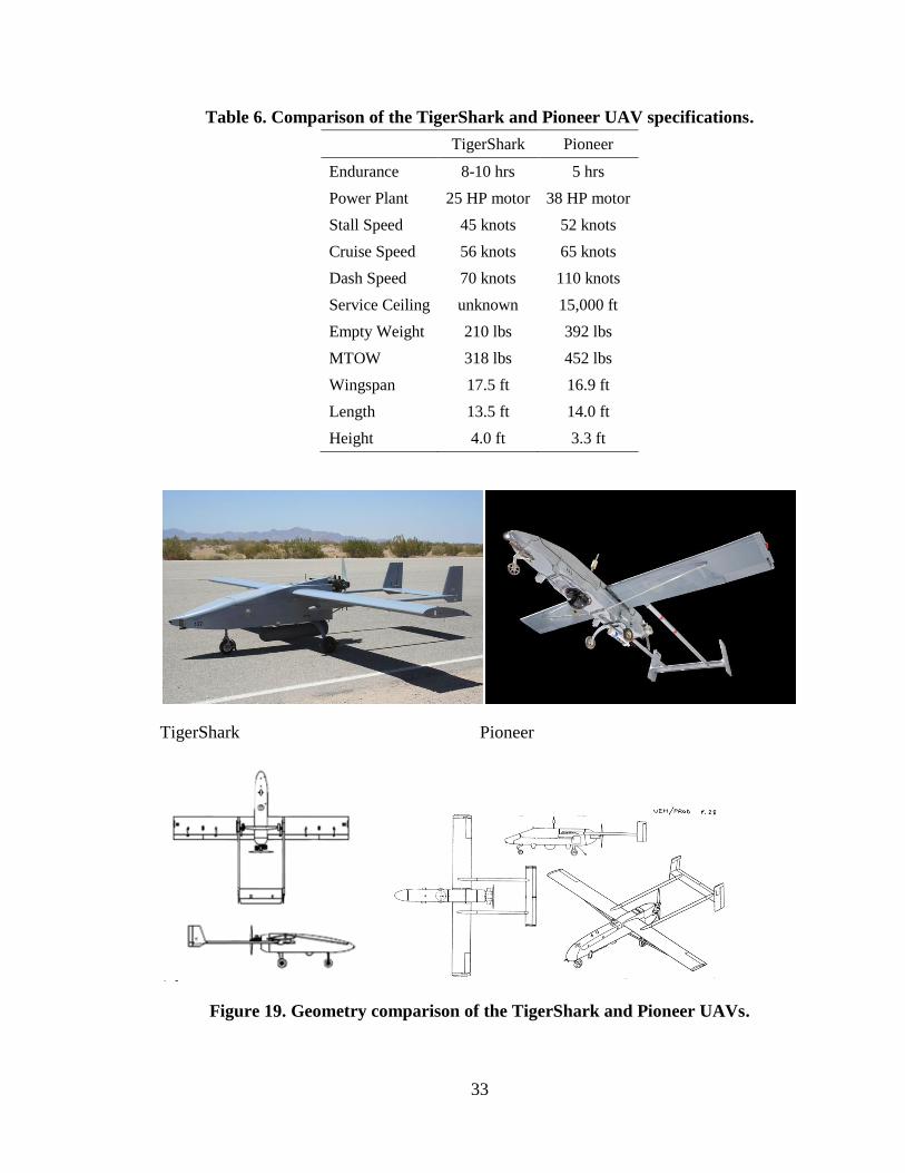
similarity of TigerShark and Pioneer platforms. Table 6 shows the comparison of the

main characteristics of these two UAVs. It is apparent that TigerShark is lighter than

Pioneer, equipped with a less powerful engine, and generally slower. However, the

physical dimensions of both aircraft are comparable. Furthermore, as shown in Figure 19,

the geometry of Pioneer and TigerShark is very similar. Both aircraft feature rectangular

wing, similar fuselage with pusher motor, twin booms, tricycle undercarriage and an H-

tail.

33

Table 6. Comparison of the TigerShark and Pioneer UAV specifications.

TigerShark Pioneer

Endurance 8-10 hrs 5 hrs

Power Plant 25 HP motor 38 HP motor

Stall Speed 45 knots 52 knots

Cruise Speed 56 knots 65 knots

Dash Speed 70 knots 110 knots

Service Ceiling unknown 15,000 ft

Empty Weight 210 lbs 392 lbs

MTOW 318 lbs 452 lbs

Wingspan 17.5 ft 16.9 ft

Length 13.5 ft 14.0 ft

Height 4.0 ft 3.3 ft

TigerShark Pioneer

Figure 19. Geometry comparison of the TigerShark and Pioneer UAVs.

34

4.4.2 Geometric Analysis Using AVL

The geometry of the TigerShark UAV was analyzed with the use of AVL software in a

similar manner as the geometry of the Pioneer aircraft. The dimensions in the main

geometry input file were modified to match TigerShark's dimensions as closely as

possible. A visualization of the resulting geometry is shown in Figure 20.

Figure 20. AVL visualization of the TigerShark UAV model.

4.4.3 Corrected Analysis Using Pioneer Correction Factors

Given the similarity of the Pioneer and TigerShark designs, it can be reasonably assumed

that the inherent errors in the AVL analysis should be similar for both vehicles. These

errors are described numerically, using the correction factor table shown in Table 5. As

described in detail in section 4.3.4, the correction factors allow us to update the

coefficients, obtained from the AVL analysis, to more realistic values. Hence,

multiplying the results of the TigerShark AVL analysis by the Pioneer correction factors

shall lead to more accurate modeling of the TigerShark dynamics. Table 7 shows the

resulting coefficients, which were implemented in the TigerShark model.

35

Table 7. Corrected AVL analysis of the TigerShark UAV.

Coefficient Pioneer

AVL

Pioneer Wind

Tunnel

Correction Factor

TigerShark AVL

Corrected TigerShark

A

oA

6-d

eg CL 0.849 0.945 1.113 0.816 0.908

CD 0.090 0.09 1.000 0.0730 0.073

Cm 0.234 0.012 0.051 0.0762 0.004

Lon

gitu

din

al

CL0 0.285 0.385 1.351 0.306 0.413

CLα 5.39 4.78 0.887 4.87 4.32

CLδe 0.571 0.401 0.703 0.395 0.278

CD0 0.065 0.06 0.923 0.035 0.032

CDα 0.239 0.43 1.801 0.267 0.482

CDδe 0 0.018 +.018 0 0.018

Cm0 0.223 0.194 0.870 0.0231 0.0201

Cmα -2.13 -2.12 0.996 -0.507 -0.505

Cmq -30.7 -36.6 1.192 -9.92 -11.8

Cmδe -2.28 -1.76 0.772 -1.11 -0.857

Late

ral

Cyβ -0.577 -0.819 1.419 -0.345 -0.490

Cyδr 0.351 0.191 0.544 0 0.00

Clβ -0.056 -0.023 0.411 -0.0681 -0.0280

Clp -0.557 -0.45 0.808 -0.503 -0.406

Clr 0.220 0.265 1.205 0.210 0.253

Clδa -0.203 -0.161 0.794 0.211 0.167

Clδr 0.00 -0.00229 -0.00229 0 -0.00229

Cnβ 0.125 0.109 0.870 0.0659 0.0573

Cnr -0.168 -0.2 1.192 -0.0820 -0.0978

Cnp -0.078 -0.11 1.419 -0.0612 -0.0869

Cnδr 0 -0.0917 -0.092 0 -0.0917

Cnδa 0.0048 0.0200 4.206 -0.000630 -0.00265

36

4.5 OX UAV

The dynamic aircraft model for the OX aircraft is the most sophisticated newly designed

model implemented within the UAV simulation environment. According to the

manufacturer, CLMax Engineering, the OX UAV is a low-cost platform, which offers

great versatility13

. It allows for various types of payload, which can be either carried

internally, or on two under-wing hardpoints. Asymmetric payloads are acceptable up to

20 pounds. Table 8 shows the main parameters of the OX UAV. Note that it is assumed

that fuel tanks have enough volume to hold fuel up to maximum useful load. This

assumption is then used to calculate endurance.

Table 8. OX UAV specifications.

Parameter Value

Wingspan 15'

Length 7' 6''

Height 3'

Wing Area 24.00 ft2

MTOW 110 lbs

Endurance 8 hours

Fuel Capacity 40 lbs

Cruise Speed 41 knots

Dash Speed 65 knots

4.5.1 Geometric Analysis Using AVL

In general, AVL analysis was carried out in a similar fashion as in the case of Pioneer and

TigerShark UAVs. However, there is one substantial difference: The OX aircraft employs

an inverted V-tail configuration. Inputting this special geometry into AVL has proven to

be exceptionally simple. Two sets of tail section coordinates were entered: one for the

outboard and one for the inboard extreme.

Control surfaces present on the V-tail can in principle be used to control two different

channels: pitch, using symmetrical deflections, or yaw, using differential deflections.

According to CLMax, the control software currently present on the aircraft only allows

pitch control using the tail surfaces (no provision for ruddervators). However, a

ruddervator control derivative was calculated for use in the UAV simulation

environment. Implementation of this control technique only requires a flight control

software upgrade, as the two tail control surfaces feature independent servos.

37

Figure 13. AVL visualization of the OX UAV model.

4.5.2 Engine Model

An accurate analysis of the aircraft dynamics requires form drag as well as thrust to be

known. However, in case of the OX UAV, neither of these parameters was readily

available from the data given. Therefore, additional information was required. CLMax

Engineering provided the author with limited flight test data, which also included a rate

of climb versus airspeed profile. This information was then used to determine thrust

available at a given airspeed as follows:

A simulation experiment was carried out to evaluate the maximum rate of climb profile

as a function of velocity. The test was started at a very low altitude, approximately 100

feet above sea level. Maximum thrust was then commanded and the pitch attitude of the

aircraft was adjusted to keep minimum permissible 1G airspeed, just above stall. The

airspeed was then slowly increased by decreasing the pitch attitude of the UAV, until

level flight was reached at maximum level flight (dash) speed. Rate of climb was then

plotted against airspeed; a quadratic curve was fitted to the data obtained as shown in

Figure 21.

38

Figure 21. Maximum rate of climb as a function of velocity simulation experiment.

The test was repeated for different weights and thrust profiles, to gain an accurate

understanding of the factors affecting rate of climb and their significance. Finally, a

thrust profile was determined by using the known brake horsepower of the engine (9 HP),

propeller dimensions (28x10, 2 blades) and drag characteristics of the aircraft.

An online static thrust calculator19

was used to find the RPM necessary to load the engine

to the maximum static horsepower. Assuming the pitch speed (propeller pitch times

RPM) is close to the dash speed of the aircraft, an RPM curve was found for the entire

speed range of the aircraft. Theoretical static thrust was also found using the online

calculator. Thrust at dash speed was found by calculating drag at dash speed using AVL.

The thrust profile was then assumed to be linear, with a decrease at low speeds due to

very low propeller efficiency at these speeds. Idle thrust was also estimated. The thrust

profile is shown both in Table 18 and, graphically, in Figure 50 in Appendix C. Finally,

the thrust profile was implemented in Simulink, using a lookup table with aircraft

velocity as an input.

The final rate of climb profile quadratic fit is shown in Figure 22, in comparison with

upper and lower bounds for maximum rate of climb, which were obtained from the flight

test data provided by CLMax Engineering.

39

Figure 22. Maximum rate of climb comparison with flight test data.

4.5.3 Stall Model

In order to allow accurate analysis of autonomous flight control algorithms at upset flight

conditions, a stall model is required. This shall ultimately enable the design of

autonomous stall recovery control laws. The stall model was designed by studying lift

and drag curves for the NACA 63-415 profile20

, which is used on the wing of the OX

UAV. The raw lift and drag data shown in Figure 23 was subsequently adjusted for wing

incidence and scaled to match the maximum lift coefficient at stall, as well as the drag

coefficient at dash speed. All data points were finally entered into lookup tables for angle

of attack contributions to lift and drag, effectively creating a stall model. Data was

duplicated for negative angles of attack down to -30 degrees as well.

Stall model, developed specifically for the OX UAV was then retrofitted to the Pioneer

and TigerShark UAV models. Adjustments were made to consider the unique wing

profiles for both Pioneer and TigerShark, and the data was re-scaled to accommodate the

most important data points: lift at maximum angle of attack and drag at dash speed.

40

Figure 23. Lift and drag curves for the NACA 63-415 profile20

.

4.5.4 Landing Gear Model

Flight control algorithms are investigated, which allow autonomous landing of the UAV.

In order to replicate the characteristics of the aircraft at touchdown and on rollout, a

landing gear model was adopted. The model architecture is based on a previous landing

gear model developed by Phil Evans for the Learjet business jet model21

. The blocks

inside the model were simplified, appropriate spring and damping constants were found,

as were wheel positions with respect to the center or gravity of the aircraft.

The landing gear model first computes the position of each tire with respect to the

ground. If the tire is in contact with ground, strut compression and lateral velocity

41

component of the tire with respect to the ground are passed to subsequent blocks, which

calculate forces acting on the corresponding tire and strut. Tire friction is calculated in

the following block. Finally, forces are added up to determine the landing gear force

contribution acting on the aircraft. Cross products of these forces with the positions of the

corresponding tires are taken to evaluate the moments acting on each wheel. Sum of these

moments is passed onto the output of the block along with the sum of the forces. The

organization of the landing gear model is shown in Figure 24.

Figure 24. Landing gear model structure.

A crash model has been implemented, which considers the position of five critical points

on the aircraft with respect to the ground. These five points are: wing tips, H-tail tips, and

nose. If any of these points becomes in contact with the ground, the simulation will stop.

This also accounts for hard landings albeit in correct aircraft attitude, because an

excessive compression of landing gear struts will cause the H-tail tips become in contact

with the ground.

Landing gear simulation involves extremely fast dynamics, which require a lower

integration step than the general simulation. To accommodate the lower integration step

in the event of ground operations, provisions were made that are described in greater

detail in section 6.2.3.

The landing gear model was implemented on Pioneer, TigerShark, and WVU YF-22

aircraft models as well. Appropriate wheel positions, spring and damping constants were

considered to customize the model for each aircraft type.

42

CHAPTER V

PATH PLANNING

The purpose of path planning algorithms is to generate a flyable path that will get the

UAV from point A to point B while accomplishing some additional tasks. Common path

planner objectives range from overflying target areas to provide surveillance and

avoiding threat zones that could harm the aircraft to extended loitering or area

reconnaissance22

.

The WVU UAV simulation environment includes path planning algorithms that can be

divided into two principal groups: obstacle avoidance techniques and point of interest

algorithms. Obstacle avoidance also refers to threat zone avoidance and risk

minimization. This chapter presents both kinds of algorithms separately; however, the

idea is to eventually join them into algorithms that will guide the aircraft to overfly the

assigned waypoints, while avoiding known threat areas and obstacles at the same time.

5.1 Obstacle Avoidance Techniques

The topic of obstacle avoidance has been extensively studied and numerous methods of

path generation are available from the literature. Three of these methods have been

implemented within the UAV simulation environment for comparison, namely Voronoi,

Grid, and Potential Field methods.

5.1.1 Voronoi

The Voronoi method23

is a modified algorithm based on the mathematical decomposition

of a given area, known as the Voronoi diagram. The Voronoi diagram takes a set of

points as an input and presents all the locations equidistant to the two nearest points.

These locations are arranged in lines as shown in Figure 25. The points represent centers

of threat zones, which we want to avoid. The Voronoi method then uses an optimization

algorithm to select the most favorable navigable path using the lines on the diagram.

43

Figure 25. A Voronoi Diagram24

.

As the Voronoi diagram itself does not account for threat zone radii, the optimization

function, which selects a navigable path uses not only distance, but also exposure to

threat as its cost function. The idea is that the Voronoi diagram will create a set of

potentially favorable paths and the optimization algorithm will then choose the best one.

Cost function is defined such that a threat zone with risk intensity 2 will never be crossed

(i.e. corresponding lines on the Voronoi diagram are given an infinite cost).

Finally, the selected path is smoothed at its corners to generate a flyable trajectory that

can be fed to the controllers on board of the UAV. Initial aircraft heading is taken into

consideration and a path segment is generated, which allows the aircraft to intercept the

selected valid Voronoi path.

44

5.1.2 Grid

The Grid algorithm8 is based on a rectangular grid with diagonal elements, as shown in

Figure 26. Each link is assigned a cost proportional to its length. The links inside the

threat zones (represented by blue circles) are assigned a higher cost, depending on the

risk intensity of the corresponding threat zone. This causes the cost optimization function

of the algorithm to preferably select paths that lie outside the threat zones, such as the one

shown in this example (in blue).

Figure 26. Grid algorithm visualization.

5.1.3 Potential Field

Another method, which is widely studied in literature, is the potential field25

. This

method is based on representing the current target or "goal" of the aircraft by an attractive

potential. Threats are represented by repulsive potentials. For any point in the arena, a

resulting force from these potentials can be computed as shown in Figure 27. Each

following path point is then generated in the direction of this force.

45

Figure 27. Potential field showing force vectors26

.

The algorithm includes provisions for a case when the magnitude of the resulting force

may become close to zero. In this case the path is deviated in a constant distance around

the nearest obstacle. Furthermore, larger threat zones are represented by numerous

repulsive obstacles around their circumference. Finally, the resulting path is smoothed in

order to become flyable.

5.2 Point of Interest Algorithms

The task of the so-called "point of interest" algorithms is to take the aircraft to one or

more target areas and return it back to the base or other landing area. This appears to be a

relatively simple objective; however, depending on the precision, which is required to

overfly the targets, sophisticated algorithms may be necessary to accomplish the task.

Generally, the intention is to minimize the overall length of the trajectory required to

achieve the objective. This saves flight time, as well as fuel, allowing the UAV operator

to survey more targets with the same resources.

5.2.1 Traditional Algorithms

Given the widespread use of point to point navigation, there are numerous point of

interest algorithms available in the literature. One of these algorithms, designated "Point

of Interest Advanced"8, was selected to provide a basic reference for this category of

algorithms in the UAV simulation environment.

46

5.2.2 Shortest Path Justification

A new algorithm for navigation via fly-over waypoints is under development. Its

objective is to generate the shortest flyable trajectory, which would cross a given set of

waypoints in a given order. Flyable trajectory is defined as trajectory with a minimum

radius of curvature equal to the minimum turn radius R of the aircraft at a given cruising

speed. As discussed above, the main optimization criterion for point of interest

algorithms is the length of the trajectory, which has to be minimized. Ultimately, this

problem shall be solved for a trajectory with n waypoints.

However, for simplicity, let's first consider a sequence of three waypoints. Assuming that

the aircraft leaves waypoint 1 at the most convenient heading, starts a turn towards

waypoint 3 and crosses waypoint 2 in the process of this turn. Refer to Figure 28 for a

visualization of the geometry.

The trajectory flown by the aircraft is shown in green, while blue segments represent the

straight line distances between the waypoints. The required turning angle between the

two segments is designated θ. There are an infinite number of trajectories, which satisfy

the geometry shown in Figure 28. Let's define "Advance Turn Ratio" or x (0 ≤ x ≤ 1) to

distinguish among these trajectories. A decision has to be made, whether it is better to

start the turn upon crossing waypoint 2 (x = 0), complete the turn by waypoint 2 (x = 1),

or cross waypoint 2 at some stage during the turn (0 < x < 1). The goal is therefore to

select an x, such that the overall length of the trajectory is minimal.

An equation was developed, which evaluates the optimum value of x, based on three

parameters: L1/R, L2/R and the turning angle θ. Dividing by the turning radius non-

dimensionalizes the segment lengths and eliminates the need for an additional parameter.

The following equation was created using Figure 28 as a guide:

√ ( ) √

(( ) )

where:

(

√ ( )

) ( ( )

√ ( )

)

(

√ (( ) ))

(

( )

√ (( ) ))

To non-dimensionalize the equation, both sides were divided by R. A MATLAB code

was then used to find the Advance Turn Ratio (x) as a function of L1/R, L2/R and θ.

47

Figure 28. Shortest flyable path geometry.

A plot of the Advance Turn Ratio versus L1/R and L2/R is shown in Figure 29. Note that,

as the segments become longer, or their lengths become more equal, the optimum

Advance Turn Ratio becomes closer to 0.5. This corresponds to crossing waypoint 2 at

the half-point of the turn.

48

Figure 29. Advance turn ratio as a function of segment lengths for θ = 90°.

The initial development version of a point of interest algorithm, which seeks the shortest

possible path with the help of the above results, is available in the UAV simulation

environment and is designated POI v1. The implementation of the geometry described

above is done using a MATLAB script. The inputs to the algorithm are present aircraft

position and velocity vector, as well as locations of all waypoints. The last waypoint is

considered the end of the trajectory. The user (or higher-level algorithm) has the option to

specify a given heading, at which each waypoint is to be crossed. If no heading is

specified, the POI v1 algorithm will assign an optimum heading. The optimum heading

computation for the nth waypoint is simply the average between the bearing from (n-1)th

waypoint to the nth waypoint and the bearing from the nth waypoint to the (n+1)th

waypoint. This corresponds to an Advance Turn Ratio equal to 0.5. A future expansion of

the algorithm will consider the Advance Turn Ratio graph in Figure 29 to determine the

optimum waypoint crossing heading.

Once all waypoint crossing headings have been established, the algorithm considers the

segments between every two waypoints separately. The algorithm contains a loop, which

generates trajectory points for each time step, one by one. The first and last trajectory

49

points are given by the start and end of the segment. Each segment is assigned a “forward

path vector” positioned at the start and a “reverse path vector” positioned at the end.

These vectors have a magnitude equal to the planned ground speed of the UAV. The

direction of the “forward path vector” is given by the waypoint crossing heading for the

first waypoint, while the “reverse path vector” has the opposite direction to the waypoint

crossing heading for the second waypoint of the segment. For each loop cycle, a new

trajectory point is either added to the beginning of the trajectory (forward path) or the end

of the trajectory (reverse path). Each subsequent trajectory point is added in the direction

of the forward or reverse path vector and distance corresponding to the magnitude of the

corresponding vector multiplied by the integration step. The vector direction is then

adjusted to the left or right by the turning angle ε, which is the maximum angle that the

aircraft can turn in one integration step. The procedure used to determine whether the

next trajectory point will be added to the forward path or reverse path and the direction of

the turn, by which the corresponding vector shall be adjusted is shown in the flowchart in

Figure 30.

START

DONE

α > β? NoYes

α > ε or β > ε?

Generate straight

line segment

NoYes

Turn required

to reduce α

Turn required

to reduce β

Increase forward

path vector

heading by ε

Decrease forward

path vector

heading by ε

Left

Right

Increase reverse

path vector

heading by ε

Decrease reverse

path vector

heading by ε

Left

Right

Continue on

forward path

Continue on

reverse path

Figure 30. Turn generation flowchart.

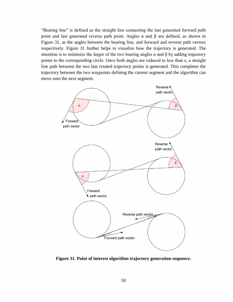
50

“Bearing line” is defined as the straight line connecting the last generated forward path

point and last generated reverse path point. Angles α and β are defined, as shown in

Figure 31, as the angles between the bearing line, and forward and reverse path vectors

respectively. Figure 31 further helps to visualize how the trajectory is generated. The

intention is to minimize the larger of the two bearing angles α and β by adding trajectory

points to the corresponding circle. Once both angles are reduced to less than ε, a straight

line path between the two last created trajectory points is generated. This completes the

trajectory between the two waypoints defining the current segment and the algorithm can

move onto the next segment.

Figure 31. Point of interest algorithm trajectory generation sequence.

51

CHAPTER VI

TRAJECTORY TRACKING

The objective of trajectory tracking algorithms (or controllers) is relatively simple: to

match the trajectory actually flown by the aircraft with that planned by trajectory

planning algorithms. However, this task may become extremely complex when adverse

conditions, such as weather or failures, introduce deviations and errors.

Trajectory tracking algorithms require a correctly formatted trajectory as their input.

Section 6.2.1 describes the format used. Controllers also require the knowledge of some

aircraft states at each time step. As a minimum, current position and velocity of the UAV

has to be known. This can also be complemented by direct input from aircraft sensor

inputs, such as altitude and velocity magnitude measurement (Pitot and static probes),

Euler angles and angular rates (gyroscopes), as well as horizontal position (GPS

receiver).

The job of the trajectory tracking algorithms is to process the above information and

generate stick (pitch and roll), rudder (yaw), and throttle (thrust) commands that would

produce the desired trajectory. This chapter describes the methods, which are used in the

UAV simulation environment, to achieve this objective.

6.1 Path to Trajectory Conversion

There are several geometry-oriented path planning algorithms in the UAV simulation

environment, which first generate a geometric path and require a subsequent conversion

to a discrete trajectory. These path planners therefore incorporate a conversion script,

which takes straight lines and arches produced by the algorithms and converts these

shapes to a sequence of three-dimensional position commands. The velocity components

are then calculated using a dedicated Simulink block, which takes the time derivative of

the commanded position.

52

6.2 Simulink Implementation

6.2.1 Trajectory Definition

The trajectory is defined by a position and velocity command vector at each time step.

This vector can be produced by loading a trajectory file, by creating the appropriate

command using an s-function, or by manually flying a "leader aircraft" and using its

position and velocity as the command vector. The required format for the trajectory file is

shown in Table 9. The box represents the actual contents of the trajectory file.

Table 9. Trajectory file format.

Position Coordinates [m] Velocity Components [m/s]

X Y Z X Y Z

Time … … … … … …

↓ … Trajectory File Contents … … … … … … …

6.2.2 Simulation Run Time

In order to facilitate the processing of simulation results, it is required that the simulation

automatically terminates once the UAV reaches the end of the commanded trajectory. A

MATLAB script was designed to set the simulation run time to one of the following:

a) Time required to run a pre-recorded trajectory or a trajectory computed by POI v1

or POI v2 algorithms. These trajectories are loaded from files, which contain a

time vector.

b) Infinite time for manual flight (simulation is stopped by user) or trajectories

created by s-functions (simulation is stopped by a dedicated Simulink block). The

"Stop Simulation" block activates whenever all commanded velocity components

are zero. This happens at the end of s-function generated trajectories.

6.2.3 Simulation Integration Step

The selection of simulation integration step is a balance between the accuracy of the

results obtained and the amount of computing power required to run the simulation. Since

the UAV simulation environment is a highly flexible multi-purpose platform, the

optimum integration step varies depending on the task. If the user wishes to perform an

autonomous landing, for example, a small integration step is required to accurately

simulate the landing gear dynamics. If, on the other hand, a complex mission is to be

analyzed, a larger integration step is preferable to allow for time acceleration.

53

The integration step is chosen automatically using a MATLAB script, once the user starts

the simulation. The script considers the algorithms chosen, as well as the selection of real

versus accelerated time. The integration step range is between 0.004 seconds for landing

gear dynamics modeling and 0.02 seconds for maximum time acceleration. Note that all

trajectories are stored with a 0.02 second time step, hence 0.02 has to be a multiple of the

selected integration step whenever a trajectory is to be loaded. This permits the choice of

0.004, 0.005, or 0.01 integration steps.

6.3 Trajectory Tracking Algorithms

This section describes the current selection of trajectory tracking algorithms available in

the UAV simulation environment. The controllers are presented in increasing level of

complexity, and only new additions to the respective algorithms are presented in each

sub-section.

6.3.1 Heading PID

The heading proportional-integrator-derivative (PID) controller is the simplest trajectory

tracking algorithm available in the UAV simulation environment. It computes the

heading required to reach the commanded horizontal position and it also evaluates the

vertical (altitude) error. The heading error information is then used to directly produce

aileron and rudder inputs. Pitch angle to capture and hold the desired altitude is

calculated from vertical error. Desired and actual pitch angles are then compared to

produce elevator input. Longitudinal error is minimized by throttle control. If the vertical

error exceeds a pre-determine threshold, airspeed is controlled by pitch and thrust is

either set to maximum or idle, depending if the aircraft is below or above the desired

altitude respectively.

6.3.2 Position PID

The Position PID27

controller, is based on minimizing the errors in the position and

velocity vector components in the Cartesian coordinates. Desired position and velocity

vectors are obtained from the trajectory command. They are compared with aircraft

sensor (GPS) readout and the errors in aircraft body axes are computed and passed onto

the outer loop controller. This is a PID controller, which determines the required bank,

pitch and thrust values to correct for lateral, vertical and longitudinal errors respectively.

Finally, the inner loop controller (also a PID) determines the actuator and throttle

commands required to achieve these values. To do this, current Euler angles and angular

rates are obtained from the aircraft gyros. Figure 32 summarizes the main components of

the Position PID controller and explains their interactions.

54

Figure 32. Position PID controller schematic.

6.3.3 Outer Loop NLDI

The non-linear dynamic inversion (NLDI) outer loop controller28

applies the NLDI

principle to roll (bank angle) and thrust control in the outer loop. The idea is to use

previous knowledge of the aircraft model, namely lateral-directional stability derivatives,

drag and thrust profiles, to estimate the bank angle and thrust required to accurately

follow the commanded trajectory. This requires inverting a part of the original aircraft

model. PID control is still used in the inner loop, as well as to determine the commanded

pitch angle in the outer loop.

6.3.4 Extended NLDI

In addition to the Outer Loop NLDI control described above, the Extended NLDI

controller29

features full NLDI control on all channels in the inner loop. A quick

comparison of the Outer Loop NLDI and Extended NLDI controllers can be seen in

Table 10.

Table 10. Outer loop NLDI and extended NLDI controller comparison.

Outer Loop NLDI Controller

Extended NLDI Controller

Pitch Roll Thrust

Pitch Roll Thrust

Outer PID NLDI NLDI

Outer PID NLDI NLDI

Inner PID PID

Inner NLDI NLDI

Elevator Aileron Throttle

Elevator Aileron Throttle

55

The inner loop NLDI control is further divided into "slow" and "fast" modes. Slow mode

NLDI processes Euler angle errors and computes desired angular rates to eliminate these

errors. Fast mode NLDI is composed of two modules. The first one evaluates the

moments necessary to produce the desired angular rates. Finally, the second module

calculates the required actuator commands to produce these moments, as well as the

required throttle setting to produce the desired thrust force.

6.3.5 LQR

The linear-quadratic regulator (LQR) is the solution to an optimum control problem,

which employs state-space representation to compute optimal gains for both lateral and

longitudinal control in the inner loop. This controller can be used when linear

mathematical model of the aircraft is known. The state-space model for the WVU YF-22

aircraft was obtained from flight tests carried out by Dr. Napolitano and his team30

.

Lateral and longitudinal control gains are then used to determine elevator, aileron, and

rudder control inputs, knowing commanded pitch and bank angles, aircraft velocity, angle

of attack, sideslip angle, Euler angles, and angular rates. Outer loop, as well as throttle, is

controlled using PID.

6.3.6 Adaptive Algorithms

Fault tolerant flight control design requires the use of adaptive elements28

, which can

respond to previously unknown dynamic characteristics of the aircraft, even after one or

more failures have occurred. In the UAV simulation environment, adaptive versions have

been created for the Heading PID, Position PID, Outer Loop NLDI, and Extended NLDI

controllers. The intention is to improve controller performance under nominal conditions,

and, above all, successfully control the aircraft under abnormal (failure) conditions.

The adaptive elements used in the UAV simulation environment are implemented in the

inner loops of the controllers listed above. Briefly said, the adaptive elements sense the

rate of increase/decrease in the Euler angle errors. They then artificially scale these errors

to produce required control response. For example, if an unexpectedly large bank angle

error occurs, the adaptive element will artificially increase the size of this error,

prompting a stronger aileron response. This principle is taken to another level in the case

of the adaptive version of the Extended NLDI controller, where adaptive elements are

used to scale angular rates, rather than Euler angles.

The adaptation law is based on a mechanism inspired by the operation of the immune

system28

.

56

6.3.7 Simulink Implementation

All nine controllers described above are implemented in parallel in the Simulink models

for each aircraft. However, in order to minimize the necessary computing power and time

necessary to run an accelerated-time simulation, at most one controller is active at a time.

This is done by the use of "Enabled" Simulink blocks, as shown in Figure 33. Output of

disabled blocks is multiplied by zero to prevent spurious control inputs. Any controller

can be easily upgraded or replaced, by simply replacing its respective Simulink block.

Figure 33. Simulink implementation of trajectory tracking algorithms.

57

6.4 Formation Flight

The UAV simulation environment includes a provision for formation flight, where one

aircraft (called leader) is flown manually and another aircraft (called follower)

automatically keeps its position in a formation. The scenario can easily be expanded to a

formation of more than two aircraft, if necessary. The purpose of the formation flight

option is to allow users to instantly evaluate the performance of trajectory tracking

algorithms in response to custom maneuvers. The alternative would be to save a manually

flown trajectory and subsequently re-load it as an input for autonomous flight.

Trajectory of the leading aircraft (3-D position and velocity components) is fed to the

controller on board of the trailing aircraft with a time delay. This effectively causes the

following aircraft to fly a fraction of a second behind the leader. Longitudinal, lateral,

and vertical spacing in leader's body axes can also be specified. However, if a large

spacing is selected, this method could potentially cause issues in sharp maneuvering

flight, when the leader's body axes turn at a large angular rate, causing the commanded

position for the follower to swing around rapidly. Hence the time delay method is

preferred.

Trajectories of both aircraft in formation flight can be visualized using the UAV

Dashboard. Furthermore, two FlightGear windows are presented to the user. Both

windows show both aircraft in the formation; however, one FlightGear window is

centered on the leader, while the other is centered on the follower. Corresponding air data

parameters (airspeed, altitude) are also presented on the respective HUDs. A schematic of

the formation flight setup is presented in Figure 34.

Figure 34. Formation flight schematic.

58

Figure 35 shows a pair of YF-22s engaged in a formation flight. The aircraft in front is

the leader, flown manually by the user, while the trailing aircraft is the follower. The

upper image is taken from the leader's FlightGear presentation, while the lower image is

from the follower's FlightGear window.

Figure 35. YF-22s flying in formation.

59

CHAPTER VII

ABNORMAL CONDITIONS

The WVU UAV simulation environment is designed to facilitate innovations in trajectory

planning and tracking algorithms, especially with respect to flight under failure

conditions. In order to allow for realistic testing under abnormal conditions, extensive

system failure options are available. Certain path planning algorithms also have

provisions for a trajectory re-plan, in case an abnormal condition occurs. Finally, an

algorithm was created, which allows autonomous landing of the UAV at the most

convenient landing facility. This may be extremely useful in serious emergencies.

7.1 Failures

There are currently two aircraft in the UAV simulation environment, which feature

failure models: the WVU YF-22 and NASA GTM. Both models feature control surface

failures. In addition, the GTM includes some structural failures and the YF-22 simulates

gyro sensor failures.

7.1.1 Structural

Structural failures represent damaged or missing pieces of the aircraft structure, which

affect aerodynamics and therefore handling qualities of the aircraft. In simulation, this is

accomplished by altering the corresponding stability and control derivatives.

There are 6 types of structural failures available in the GTM model: missing rudder,

vertical tail, outboard flap, wingtip, elevator, or stabilizer. Each of these failures affects

respective stability (and/or control) derivatives. The contribution of each failure is

evaluated using look-up tables inside the NASA GTM aerodynamic model.

60

7.1.2 Controls

Control surface failures can create a significant challenge for the autonomous flight

control systems. Therefore, numerous control failures are implemented in the UAV

simulation environment. These range from missing control surfaces to surfaces stuck at a

specific control deflection.

Missing parts of control surfaces are simulated by multiplying the respective control

derivative by the percentage of the remaining surface. Stuck control surfaces are

simulated by replacing the controller (or joystick) input by an imposed value. This value

may either be pre-selected by the user or the control surface may become stuck at

"current deflection", meaning the control surface deflection at the instant of the failure.

7.1.3 Sensors

The UAV simulation environment features gyro sensor failures. These sensors measure

angular rates p, q and r. At the moment of a failure, a bias is introduced in the sensor

reading. This can cause certain types of trajectory tracking algorithms to compensate for

a non-existing angular rate.

Furthermore, small level of noise is introduced to all sensor readings. Additional sensor

degradation can be simulated by using a dedicated sensor block. Provisions for probe

icing or contamination are included. Future expansion of the UAV simulation

environment will include more detailed models of sensor failures including GPS.

7.2 Mission Re-plan

Even the best plans sometimes fall apart. Traditionally, it was the job of human operators

to manually guide the UAV in these situations and decide on an alternate plan. However,

given the complexity of future UAV missions, as well as the fact that the human pilot is

not on board of the aircraft and that communications can be jammed, it is essential that

the future generations of UAVs be able to accommodate for a mission re-plan.

7.2.1 Tactical Re-plan

A tactical re-plan generally involves changing the trajectory, perhaps to avoid a newly

discovered threat zone, include a new target in the surveillance, or to recover the aircraft

at the nearest landing facility, if the situation requires. In order to be able to decide when

a re-plan is necessary, the UAV needs to be equipped with sensors that will detect

61

significant changes in the outside environment, or at least with a communication link that

will allow the operator to order a re-plan.

In the UAV simulation environment, there are four s-function based trajectory planning

algorithms (Voronoi, Grid, Point of Interest, and Potential Field) that already have a

provision for tactical re-plan. This is done via a "recalculate" signal, which can prompt

the algorithm to generate a new path, if the aircraft suffers a failure, mission objectives

are changed, or a new threat is detected. Future expansions of the simulation environment

will include triggers, which will decide when a re-plan is necessary and what the new

objectives should be.

7.2.2 Diversion to Nearest Runway

In case that the aircraft is damaged during the mission, its fuel status unexpectedly

declines or there is any other serious emergency, the best course of action is to recover

the UAV at the nearest available landing facility. For this reason, a dedicated trajectory

planning algorithm has been developed, which will automatically select the most

appropriate runway, and guide the aircraft to an autonomous landing. Thus, in theory, the

UAV can recover itself even when its communication links with the ground control

station are severed.

The trajectory is generated as follows. Coordinates of the touchdown point are loaded

from a runway database. This point is defined as the last point of the trajectory. The

coordinates of each previous point are computed by subtracting the velocity vector from

the current point's coordinates. This creates a so called "reverse path" as shown in Figure

36. A straight portion of the reverse path is generated first, which allows a safe final

descent of the aircraft that would clear any obstacles that may lie outside of the runway

centerline. The beginning of the straight reverse path portion is called a "gate". The

minimum height of the gate above runway elevation can be specified by the user as a

parameter of the trajectory generation algorithm.

Next, a short straight portion of the forward path is generated in a similar manner. Present

aircraft position (or the position of the last point of the previously generated trajectory in

case of a pre-planned diversion) is used as a starting point for the forward path. The

purpose of the straight portion is to stabilize the aircraft after any previous maneuvering.

62

Figure 36. Automatic approach to landing geometry.

Now, the forward and reverse path segments need to be oriented so as to allow a

connection. This is done using the same logic as described in section 5.2.2 and shown in

the flowchart in Figure 30. Since the trajectory planner requires fairly limited

computational power to achieve a solution, trajectories are computed to all available

runways at several nearest landing facilities. Once the solutions are obtained, the shortest

trajectory is chosen.

Finally, the vertical path is calculated in reverse direction, starting from the touchdown

point and ending with the initial trajectory point. Appropriate rate of descent is planned to

incorporate the flare maneuver, slow final descent used to slow the aircraft from approach

speed to touchdown speed and a constant speed descent. Once the initial aircraft altitude

is reached, the trajectory planner will plan for level flight until the initial trajectory point

is reached.

In case the vertical trajectory planner does not reach a solution (the trajectory is too short

to allow for a constant speed descent, speed reduction segment and flare), the trajectory

has to be extended. This is done by arbitrarily extending the straight reverse path segment

63

(i.e. moving the gate farther from the touchdown point) in 100-meter increments until the

trajectory is sufficiently long to allow a continuous descent.

In the future versions of the automatic diversion and approach algorithm, additional

factors will be considered for runway selection. Each runway within the range of the

UAV will be assigned an additional cost index (in meters). A cost index (or penalty) of 0

will be assigned to the runway originally planned for the mission. A cost function, based

on crosswind or tailwind component, unavailability of maintenance facilities for the

UAV, or other tactical factors, will calculate the cost index for the remaining runways.

This cost index will be added to the trajectory length computed for each runway, and the

runway with the shortest "total trajectory length" will be chosen for landing in the event

of a diversion. Cost index may be variable in time, as the weather (wind direction and

strength) and tactical situation change.

64

CHAPTER VIII

SIMULATION RESULTS

An example comparison study was carried out to demonstrate the use of the UAV

simulation environment for performance evaluation of path planners and flight control

algorithms. The employment of relevant features of the simulation environment is

described in this chapter. The results obtained from the simulation are then discussed and

explained. The objective of this chapter is to aid future users in designing and executing

similar simulation experiments.

The study is composed of two independent parts. First, a hypothetical mission scenario

was given to the available path planning algorithms and the resulting trajectories were

compared on the basis of overall length and threat exposure. Secondly, a sample

trajectory was flown using the manual flight option, and a task to follow this trajectory

was given to the trajectory tracking algorithms. The algorithms were then compared

based on several metrics. Note that only one mission scenario was used for the path

planning algorithm comparison, and only a single trajectory was used for trajectory

tracking comparison. This means that results obtained from this study are by no means

conclusive and are only presented to illustrate the capabilities of the simulation

environment.

8.1 Obstacle Avoidance Path Planner Comparison Study

The four obstacle avoidance algorithms currently included in the UAV simulation

environment were compared in a limited study, which evaluated their performance and

practicality. A realistic scenario with threat distribution corresponding to simulated AAA

and short-range SAM positions was prepared using the UAV Dashboard interface.

Starting point was given the coordinates [0,0], while the goal was set at [5000,3000].

First of all, the appropriate metrics to be compared were selected. The main requirement

for the design obstacle avoidance path planners is that they actually avoid the threat

65

zones, or at least minimize the exposure of the aircraft to threats. In our study, a

subjective metric "Threat Exposure Risk" is used to evaluate the path planners'

performance in this aspect. Threat exposure risk can be "none" if the UAV never flies

through a threat zone, "low", "medium", or "high".

All path planners strive to minimize the length of the trajectory, to minimize flight time

and fuel requirements to accomplish a given mission. Therefore, "Trajectory Length"

metric was used in the comparison study. Since flight at a constant airspeed is considered,

trajectory length is also proportional to flight time. Note that the WVU YF-22 aircraft

was used for this experiment. The cruising speed of this aircraft is 80 knots.

Finally, an important consideration for the path planner comparison would be computing

time required to reach a solution. However, despite the relative complexity of the

scenario evaluated, the computing time was so short that no reasonable comparison could

be made. It is, however, a metric that shall be used in future, more advanced, analyses.

First, the Voronoi algorithm was tested. Red lines in Figure 37 represent the links in the

Voronoi diagram, which was calculated by the path planner.

Figure 37. Voronoi diagram featuring obstacle shapes and selected path.

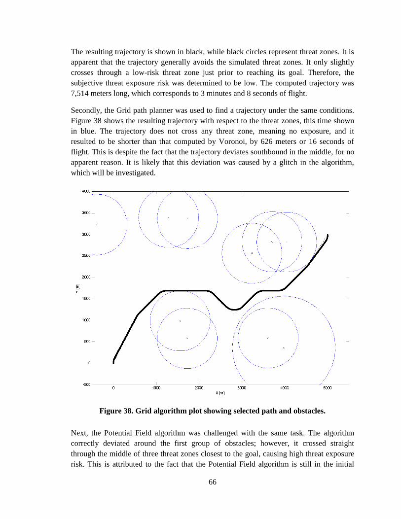
66

The resulting trajectory is shown in black, while black circles represent threat zones. It is

apparent that the trajectory generally avoids the simulated threat zones. It only slightly

crosses through a low-risk threat zone just prior to reaching its goal. Therefore, the

subjective threat exposure risk was determined to be low. The computed trajectory was

7,514 meters long, which corresponds to 3 minutes and 8 seconds of flight.

Secondly, the Grid path planner was used to find a trajectory under the same conditions.

Figure 38 shows the resulting trajectory with respect to the threat zones, this time shown

in blue. The trajectory does not cross any threat zone, meaning no exposure, and it

resulted to be shorter than that computed by Voronoi, by 626 meters or 16 seconds of

flight. This is despite the fact that the trajectory deviates southbound in the middle, for no

apparent reason. It is likely that this deviation was caused by a glitch in the algorithm,

which will be investigated.

Figure 38. Grid algorithm plot showing selected path and obstacles.

Next, the Potential Field algorithm was challenged with the same task. The algorithm

correctly deviated around the first group of obstacles; however, it crossed straight

through the middle of three threat zones closest to the goal, causing high threat exposure

risk. This is attributed to the fact that the Potential Field algorithm is still in the initial

67

stages of its development. Length of the computed trajectory was 6,753 meters and it

took 2 minutes and 49 seconds to fly.

Finally, the POI v2 path planning algorithm was used. This is an experimental algorithm,

which simply evaluates the shortest path from start to goal. If the path crosses any

obstacles, the algorithm will evaluate two options: deviate to the right or to the left

around the obstacle. It will then select the shorter option and re-evaluate the trajectory,

until all obstacles are avoided. Figure 39 shows the trajectory generated by this path

planner, as presented through the UAV Dashboard interface. With 6,602 meters, or 2

minutes and 41 seconds of flight time, it turned out to be the shortest from all simulated

trajectories. It also clearly avoids all threat zones, eliminating any exposure risks.

Figure 39. POI v2 path visualization through UAV Dashboard.

To summarize, the obstacle avoidance path planner comparison study results are

presented in Table 11. Throughout the entire testing, the use of UAV simulation

environment has proven to be easy, fast, and user-friendly. Accelerated time option was

used for the simulations. Once the scenario was set up in UAV Dashboard, a simple

switch to the next path planning algorithm was required for each subsequent test.

Trajectory lengths and en-route times were recalled from the MATLAB workspace.

68

Table 11. Obstacle avoidance path planner performance metrics comparison.

Obstacle Avoidance Comparison

Trajectory Length

[m]

Actual Enroute Time

[min, sec]

Threat Exposure Risk

Pat

h P

lan

ner

s Voronoi 7514 3 min 8 sec low

Grid 6888 2 min 52 sec none

Potential Field 6753 2 min 49 sec high

POI v2 6602 2 min 41 sec none

8.2 Controller Comparison Study

The second part of the study is focused on trajectory tracking algorithms and their

performance. A 200-second trajectory was manually flown using the WVU YF-22

aircraft model and recorded to be used for the comparison. The trajectory included a

maximum performance climb, at 90% power, giving only 10% margin to the controllers.

The climb segment included two turns at 75 knots and one turn at 65 knots. At the top of

climb, speed was reduced to under 60 knots and an s-turn was carried out. A descent was

then initiated and power was increased again, to test controller characteristics at high

speed of around 100 knots. Finally, an approach to landing was executed. A 2-D image of

the entire test trajectory is shown in Figure 40.

The trajectory was then re-loaded and flown using each trajectory tracking algorithm at

nominal, as well as failure, conditions. Numerical data from each simulation run was

analyzed.

8.2.1 Tracking Performance

Three metrics were selected to measure the tracking performance of the controllers. First,

"Mean Position Error" is defined as the average straight line distance from the actual

aircraft position to the commanded position in meters. This metric describes the tracking

precision of the controller. Next, "Mean Combined Stick & Rudder Deflection" in % is

the average of the magnitudes of elevator, aileron, and rudder deflections normalized by

using maximum deflections. This metric describes the intensity of actuator inputs

exhibited by the controllers. Finally, the "Throttle Rate Index" is defined as the average

throttle movement rate in % of travel per second. This metric describes the smoothness of

the thrust control.

69

Figure 40. Controller comparison trajectory 2-D visualization.

Let's start by analyzing the tracking performance of the controllers at nominal conditions.

Mean position error was the highest for regular PID controller, which is expected due to

the simple design of this tracking algorithm. The adaptive version of this controller even

caused the UAV to crash during the high-speed descent phase of the flight. This is

attributed to the fact that the controller tried to increase forward speed of the UAV by

disproportionately increasing the rate of descent. Position PID gave a drastic

improvement in mean position error from 219.83 to 16.60 meters and allowed sufficient

precision to guide the aircraft for a safe landing at the end of the experimental trajectory.

Outer loop NLDI controller further reduced the mean position error to only 1.79 meters

and the Extended NLDI was the winner in this aspect, with only 1.11-meter mean

70

position error. LQR controller lagged especially in turns at lower airspeed, resulting in a

mean position error of 32.40 meters. Except for the regular PID controller mentioned

above, adaptive versions of the controllers did not have any significant effect on tracking

precision at nominal conditions.

Mean combined stick & rudder deflection was very low in case of regular PID and LQR

controllers, with only 1.60 and 1.72 % deflection respectively. However, given the poor

tracking precision of these controllers, this does not necessarily mean any positive trend.

For Position PID and both NLDI controllers, the mean combined deflection was in the

order of 3.3 - 3.5 %, for both adaptive and non-adaptive versions. The only improvement

was noted with the adaptive Position PID controller, which exhibited 2.81% mean

combined deflection.

Smooth thrust control is essential for the implementation of controllers on board of the

actual UAV. Piston engine life is drastically reduced by abrupt throttle changes, which

can damage the counterweights on the engine's crankshaft31

, increasing maintenance

costs, as well as the possibility of an in-flight engine failure. Figure 41 shows the thrust

profile comparison between the original thrust commanded during the manual flight

portion, thrust produced by the Position PID controller, and the thrust produced by the

Extended NLDI controller. It is apparent, that Position PID controller varied the

commanded thrust smoothly, resulting in a throttle rate index as low as 1.62%/sec for the

non-adaptive version. The adaptive version achieved a mere 1.17%/sec throttle rate

index. On the other hand, Extended NLDI controller kept chasing the commanded

trajectory by applying disproportionate thrust inputs, even causing saturation at high

power settings. The corresponding throttle rate index was as high as 14.59%/sec.

Table 12 shows the entire set of results obtained in the experiment. Unsatisfactory

performance is presented in red. Mean position error is the advantage of NLDI controllers

over Position PID. However, this is achieved at the cost of larger actuator inputs and

highly insensitive throttle handling. On the other hand, Position PID achieves moderate

tracking precision with minimum throttle, stick and rudder use.

71

Figure 41. Throttle control comparison.

72

Table 12. Controller performance metrics comparison.

Controller Performance

Mean Position Error [m]

Mean Combined Stick & Rudder Deflection

[%]

Throttle Rate Index [%/sec]

Conventional Adaptive

Conventional Adaptive

Conventional Adaptive

No

Fai

lure

PID 219.83 CRASH 1.60 - 2.66 -

Position PID 16.60 16.35 3.34 2.81 1.62 1.17

Outer Loop NLDI 1.79 1.71 3.47 3.46 16.34 15.80

Extended NLDI 1.11 1.11 3.45 3.45 14.59 13.95

LQR 32.40 - 1.72 - 1.67 -

Stab

Fai

lure

(l

eft

sta

b s

tuck

at

trim

) PID 393.03 CRASH 5.06 - 4.04 -

Position PID 92.35 16.46 12.48 11.13 1.71 1.22

Outer Loop NLDI 9.69 1.99 12.26 12.43 18.47 17.31

Extended NLDI 1.12 1.11 12.58 12.79 16.55 14.92

LQR 33.97 - 9.13 - 1.74 -

Ail

ero

n F

ailu

re

(le

ft a

ilero

n s

tuck

at

10

de

gre

es)

PID 482.11 CRASH 48.67 - 2.66 -

Position PID 16.54 16.32 48.78 48.74 1.66 1.18

Outer Loop NLDI 4.13 2.46 48.80 48.77 17.51 15.79

Extended NLDI 1.17 1.11 46.01 45.71 15.49 14.13

LQR CRASH - - - - -

Ru

dd

er F

ailu

re

(lef

t ru

dd

er s

tuck

at

20

deg

rees

)

PID 313.74 CRASH 18.50 - 3.18 -

Position PID 25.83 21.15 18.74 18.59 1.95 1.28

Outer Loop NLDI 15.35 8.68 18.63 18.63 16.08 17.71

Extended NLDI 1.15 1.18 34.25 30.65 13.17 12.88

LQR 111.94 - 18.36 - 1.18 -

73

8.2.2 Failures

Flight under failure conditions was also considered in the study. Three failures were

simulated, one for each actuator control channel. Stabilator failure, which is the most

substantial control surface, was injected at trim. This failure resulted in drastic

degradation in the performance of all conventional controllers except the Extended

NLDI. Only their adaptive versions could keep similar tracking performance under

stabilator failure conditions as they did under nominal conditions. Naturally, mean

combined stick & rudder deflection was slightly higher for all controllers.

Next, aileron failure with left aileron stuck at 10 degrees of deflection was considered.

This is a relatively large deflection, causing the trajectory tracking algorithms to

command a stick input in the opposite direction. This, as expected, resulted in extremely

high mean combined stick & rudder deflection values. LQR controller was unable to

handle this failure and caused a crash of the UAV due to a complete loss of control and

separation from the commanded trajectory.

Finally, a rudder failure with left rudder stuck at a 20-degree deflection was simulated.

This failure has magnified the differences among all controller types and highlighted the

advantages of NLDI control. The Extended NLDI controller was the only trajectory

tracking algorithm that compensated by applying significant opposite rudder deflection

(note that YF-22 has a double vertical tail). This is thanks to the NLDI control in the

inner loop. All other controllers tried to compensate using opposite aileron, causing larger

mean position errors. Should the aircraft model be slightly less stable in yaw (as most

conventional UAVs are), correcting for a failed rudder (or any other directional

asymmetry) by the use of aileron would cause the aircraft to crash.

Finally, overall controller performance was calculated from the available metrics as

follows. A cost function was assigned to each metric, based on the required performance

threshold, as seen in Figure 42. For the mean position error, the threshold was selected to

be 7.8 meters, the worst case GPS accuracy at 95% confidence32

. For mean combined

stick and rudder deflection, threshold was 20%, corresponding to very high and frequent

control usage. Threshold for the throttle rate index was set at 7%/s, which corresponds to

a frequent and sudden throttle change.

74

Figure 42. Cost function in terms of required performance threshold.

The overall controller performance index (OCPI) was then calculated as:

[ ]

[ ] [ ]

[ ] [ ]

[ ]

The lower the OCPI, the better the controller. Table 13 shows the results of the overall

controller performance for all available controllers. It is apparent that adaptive controllers

in general have better performance than conventional ones. Best controllers are shown in

dark green. Best conventional controllers are shown in light green.

The best controller in terms of OCPI was the Extended NLDI in most cases. Adaptive

version of the Position PID exhibited better performance under stabilator failure

conditions only. As all OCPI's are larger than 3.0, none of the controllers was able to

achieve at least the required performance thresholds in all metrics. If the throttle control

of the Extended NLDI controller was optimized, its overall performance ranking could

significantly improve.

75

Table 13. Overall controller performance comparison.

Overall Controller

Performance Index (OCPI)

No

Fai

lure

Stab

Fai

lure

(l

eft

stab

stu

ck a

t tr

im)

Ail

ero

n F

ailu

re

(lef

t ai

lero

n s

tuck

at 1

0 d

egre

es)

Ru

dd

er F

ailu

re

(lef

t ru

dd

er s

tuck

at 2

0 d

egre

es)

Co

nve

nti

on

al

PID 794 2539 3826 1619

Position PID 4.6 140.6 10.5 11.9

Outer Loop NLDI 5.5 8.9 12.5 10.0

Extended NLDI 4.4 6.0 10.2 6.5

LQR 17.3 19.2 - -

Ad

apti

ve Position PID 4.4 4.8 10.3 8.2

Outer Loop NLDI 5.2 6.6 11.1 8.5

Extended NLDI 4.0 5.0 9.3 5.8

76

CHAPTER IX

CONCLUSIONS

A UAV simulation environment for the design, implementation, evaluation, and

comparison of autonomous flight control algorithms was created. A two-part example

comparison study has demonstrated the convenience of the graphical user interface, depth

of realistic threat and abnormal situation modeling, as well as availability of user-friendly

analysis tools. The main contributions of the author in the development of the WVU

UAV simulation environment were the following:

An extensive graphical user interface was designed from the roots up, including

connection to FlightGear6, plots and scopes output. The parameters required to design

three new aircraft models were obtained from moments of inertia calculations, AVL18

analyses, and performance data provided by the manufacturer. New engine and stall

models were developed, and an existing landing gear model was highly modified and

adapted to the new aircraft models. A new point of interest algorithm was developed,

analyzed and implemented in Simulink. In addition, two more algorithms were created,

using the newly designed point of interest algorithm as their core: automatic landing and

an obstacle avoidance algorithm. Finally, all components developed by the author were

linked together with aircraft models, additional path planning and trajectory tracking

algorithms, developed by other authors.

It was shown that, currently, the most practical obstacle avoidance path planning

algorithm is POI v2, and the most successful trajectory tracking algorithm is the

Extended NLDI. This is thanks to its exceptional tracking precision. Adaptive elements in

flight control algorithms have shown to be useful in improving the overall controller

performance. They have proven beneficial after the onset of certain failures, especially in

the case of stuck stabilator surfaces.

77

The UAV simulation environment is a never-ending project, which has several directions

for future improvement. First of all, modular design of the whole environment can be

improved by using model libraries, which allow extremely easy and user-friendly

substitution of Simulink blocks by newer, or different, versions. Each trajectory planning

or tracking algorithm, as well as each UAV model, could become a library block. Even

inner and outer loops within the controllers could be defined as separate library entries,

allowing independent upgrades.

Secondly, POI v1 and v2 algorithms described in this thesis could be further improved to

optimize path planning. An important addition would be performance-based altitude

selection, which would take into account winds aloft, as well as mission requirements.

Sensors may be simulated in detail, generating new criteria for aircraft flight path to

accomplish realistic objectives.

Thirdly, the UAV simulation environment should be used to optimize currently available

trajectory tracking algorithms. This does not necessarily mean increasing the complexity

of these algorithms, but rather, re-evaluating the benefits and impact of each and every

component that has been tested so far. For example, gains need to be optimized to take

full advantage of the capabilities of techniques such as NLDI or adaptive components.

Finally, the UAV simulation environment shall be expanded to allow simulation of

multiple UAVs using independent, and, possibly, different, aircraft models, flight control

algorithms, objectives and threats. More detailed simulation of enemy forces and other

threats could be included.

78

REFERENCES

1 Fudge, M., Stagliano, T., Tsiao, S., “Non-Traditional Flight Safety Systems &

Integrated Vehicle Health Management Systems - Descriptions of Proposed & Existing

Systems and Enabling Technologies & Verification Methods”, Final Report, The Office

of the Associate Administrator for Commercial Space Transportation, Federal Aviation

Administration, 2003

2 ***

, “National Aeronautics Research and Development Policy”, Executive Office

of the President of the United States, National Science and Technology Council,

December 2006

3 ***

, “U.S. Army Unmanned Aircraft Systems Roadmap 2010-2035”, U.S. Army

UAS Center of Excellence, Fort Rucker, AL, 2010

4 ***

, “UAV Simulator Solutions”, H-SIM, Montesson, France, 2009.

[http://www.h-sim.com/new_uav_sims.php Accessed 3/27/12.]

5 Kim, D., Kim, D., Kim, J., Kim, N., Suk, J., “Development of Near-Real-Time

Simulation Environment for Multiple UAVs”, EUROCON 2007 The International

Conference on "Computer as a Tool", September 9-12, 2007, Warsaw, Poland

6 ***

, “FlightGear”, 2012. [http://www.flightgear.org Accessed 3/21/12.]

7 ***

, “X-Plane 10”, 2012. [http://www.x-plane.com Accessed 3/27/12.]

8 Perhinschi, M. G., Moncayo, H., Davis, J., Wilburn, B., Karas, O., Wathen M.,

“Development of a Simulation Environment for Autonomous Flight Control Algorithms”,

AIAA Guidance, Navigation, and Control Conference, August 8-11, 2011, Portland,

Oregon

79

9 Gu, Y., “Design and Flight Testing Actuator Failure Accommodation

Controllers on WVU YF-22 Research UAVs”, Ph. D. Dissertation, Department of

Mechanical and Aerospace Engineering, West Virginia University, Morgantown, West

Virginia, 2004.

10 Jordan, T. L., Langford W. M., Hill J. S., “Airborne Subscale Transport

Aircraft Research Testbed: Aircraft Model Development”, AIAA Guidance, Navigation,

and Control Conference and Exhibit, August 15-18, 2005, San Francisco, California

11 ***

, “RQ-2A Pioneer Unmanned Aerial Vehicle (UAV)”, Public Affairs Office,

Naval Air Station, Patuxent River, Maryland, February 18, 2009.

[http://www.navy.mil/navydata/fact_display.asp?cid=1100&tid=2100&ct=1 Accessed

3/21/12.]

12

***, “TigerShark Data Sheet”, Unmanned Aircraft System Solutions, L-3

Unmanned Systems, New York City, New York, January 2, 2009.

[http://www2.l-3com.com/uas/pdf_uas/tech/TigerShark.pdf Accessed 3/21/12.]

13

***, “OX Unmanned Aerial Vehicle (UAV)”, CLMax Engineering LLC, Fort

Walton Beach, Florida, 2011. [http://clmaxengineering.com/ox01.html Accessed

3/21/12.]

14 Perhinschi, M. G., Napolitano, M. R., Campa, G., Seanor, B., Gururajan, S., Gu

Y., “Development of Fault-Tolerant Flight Control Laws for the WVU YF-22 Model

Aircraft”, Proceedings of the AIAA Guidance, Navigation, and Control Conference,

August 2007, Hilton Head, South Carolina

15 Rauw, M. O., “FDC 1.2 – A SIMULINK Toolbox for Flight Dynamics and

Control Analysis”, Delft University of Technology, Delft, The Netherlands, 1998

16 Seanor, B., Campa, G., Gu, Y., Napolitano, M.R., Rowe, L., Perhinschi, M. G.,

"Formation Flight Test Results for UAV Research Aircraft Models", Proceedings of the

AIAA Intelligent Systems Technical Conference 2004 Chicago IL, AIAA2004-6251

17 Bray, R., “A Wind Tunnel Study of the Pioneer Remotely Piloted Vehicle”,

M.S. Thesis, Naval Postgraduate School, Monterey, California, June, 1991.

18 Drela, M., Youngren H., “AVL Overview”, Massachusetts Institute of

Technology, Cambridge, Massachusetts, November 4, 2007.

[http://web.mit.edu/drela/Public/web/avl Accessed 3/21/12.]

19 Füzesi, S., “Static Thrust Calculator”,

[http://personal.osi.hu/fuzesisz/strc_eng/index.htm Accessed 3/21/12.]

80

20 Bak, C., Fuglsang P., Johansen J., Antoniou I., “Wind Tunnel Tests of the

NACA 63-415 and a Modified NACA 63-415 Airfoil”, Risø National Laboratory,

Roskilde, Denmark, December, 2000.

21 Evans, P. E., “Modeling and Simulation of Tricycle Landing Gear at Normal

and Abnormal Conditions”, M.S. Thesis, Department of Mechanical and Aerospace

Engineering, West Virginia University, Morgantown, West Virginia, 2010.

22 Nehme, C. E., Cummings, M. L., Crandall, J. W., “A UAV Mission Hierarchy”,

Humans and Automation Laboratory, MIT Department of Aeronautics and Astronautics,

Cambridge, Massachusetts, December, 2006.

23 Wilburn, J., Perhinschi, M. G., Wilburn, B., Karas, O., “Development of a

Modified Voronoi Algorithm for UAV Path Planning and Obstacle Avoidance”,

Submitted to the AIAA Guidance, Navigation, and Control Conference, August 13-16,

2012, Minneapolis, Minnesota

24 Pless, R., “Lecture 16: Fortune's Algorithm and Voronoi diagrams”, CSE 546:

Computational Geometry Class Notes, Washington University, St. Louis, Missouri,

Spring 2011. [http://www.cs.wustl.edu/~pless/546/lectures/L11.html Accessed 3/19/12.]

25 Davis, J., Cole, J., Perhinschi, M. G., Wilburn, B., “Comparison of a Fuzzy

Logic Controller to a Potential Field Controller for Real-Time UAV Navigation”,

Submitted to the AIAA Guidance, Navigation, and Control Conference, August 13-16,

2012, Minneapolis, Minnesota

26

***, “Path Planning for Avoiding Obstacles”, Advanced Mechatronics Project

Team Notes, Georgia Institute of Technology, Atlanta, Georgia, Spring 2011.

[http://www.cs.wustl.edu/~pless/546/lectures/L11.html Accessed 3/19/12.]

27 Campa, G., Wan, S., Napolitano, M. R., Seanor, B., Fravolini, M. L., “Design

of Formation Control Laws for Maneuvered Flight”, The Aeronautical Journal, pg 125-

134, March 2004.

28 Moncayo, H., Perhinschi, M. G., Wilburn, B., Wilburn, J., Karas, O., “UAV

Adaptive Control Laws Using Non-Linear Dynamic Inversion Augmented with an

Immunity-based Mechanism”, Submitted to the AIAA Guidance, Navigation, and Control

Conference, August 13-16, 2012, Minneapolis, Minnesota

29 Moncayo, H., Perhinschi, M. G., Wilburn, B., Wilburn, J., Karas, O., “Extended

Nonlinear Dynamic Inversion Control Laws for Unmanned Air Vehicles”, Submitted to

the AIAA Guidance, Navigation, and Control Conference, August 13-16, 2012,

Minneapolis, Minnesota

81

30 Napolitano, M. R., “Development of Formation Flight Control Algorithms

Using 3 YF-22 Flying Models”, Final Report, April, 2005, Morgantown, West Virginia

31 Rossier, R. N., “Managing the Engine”, AOPA Flight Training, 2011,

[http://flighttraining.aopa.org/students/solo/skills/engine.html Accessed 3/31/12.]

32 ***, “Global Positioning System Standard Positioning Service Performance

Standard”, Department of Defense, September, 2008

82

APPENDIX A

UAV SIMULATION ENVIRONMENT USER GUIDE

This user guide is valid for version 1.1.7 of the WVU UAV simulation environment. To

start the simulation environment, open MATLAB and run the script “WVUUAV.m” in

the root directory of the simulation environment. Then follow the startup instructions

below:

1 Number of Vehicles GUI

A Single: One UAV simulated (or formation flight option).

B Multiple: Three OX UAVs simulated. Startup is complete.

C Push LAUNCH button.

2 General GUI

A Select Vehicle: Selects aircraft type (Simulink model to be used)

B Select Map: Only San Francisco Bay is available at the moment.

C Select Trajectory Planning Algorithm: This step is optional. If no path

planner is selected, manual flight will be selected – skip to step 2E.

D Select Conventional Controller or Select Adaptive Controller.

E Push LOAD button: Stores the selected values into a file. If new options

are selected after pushing the LOAD button, they will not be taken into

account unless LOAD button is pressed again.

F Push VISUALS button: Opens FlightGear and UAV Dashboard interfaces.

This step is optional, if the user does not require starting both FlightGear

and the UAV Dashboard.

G Push LAUNCH button.

3 Aircraft-specific GUI: Will only load for WVU YF-22 and NASA GTM.

A Select Failures as required. This step is optional.

Once the startup is complete, a Simulink model will load. Additional selections can be

made by clicking on appropriate sub-systems. Furthermore, different path planning

algorithms and controllers can also be selected by clicking on the corresponding Simulink

blocks.

83

Note that if manual flight is active, selecting a trajectory planning algorithm will

automatically select a default controller, and selecting a controller will automatically load

a default trajectory. The following color-coding is used for the Simulink block controls:

RED: Trajectory planning algorithms. Selected algorithm block turns GREEN.

MAGENTA: Trajectory tracking algorithms. Selected controller turns GREEN.

BLUE: Additional selection blocks:

o Load/Save current trajectory to/from a file.

o Show scopes or plots. Scope selection is made using a MATLAB GUI.

o Set time acceleration. With accelerated time selected, block turns RED.

o Reload the simulation. This will allow selecting different failure options.

o Select whether the aircraft will start in the air or on the ground.

Furthermore, clicking on the following icons will launch corresponding visualization:

FlightGear UAV Dashboard

Upon starting the simulation, the user shall check the MATLAB command window for

any warning messages. This window will also display the length of the selected trajectory

and estimated en-route time of the UAV. Warning messages for Grid and Voronoi

algorithms may appear in a pop-up window.

Trajectory tracking performance metrics (position error and velocity error) can be readily

seen in the main Simulink block during the simulation. Once the simulation run has been

completed, the average position and velocity errors are shown in the MATLAB command

window.

The following files contain valuable information, for post-simulation analysis:

“sensors.m” Aircraft states (actual output not distorted by sensor modeling).

“controls.m” Control inputs.

“errors.m” Controller position and velocity errors in Cartesian coordinates.

Contents of the above files are shown inside the “Output Files” block in the Simulink

aircraft models.

To close the WVU UAV simulation environment, simply close the main Simulink block,

then close MATLAB and any visualization (FlightGear or UAV Dashboard) windows

that may be open.

84

APPENDIX B

MATLAB/SIMULINK IMPLEMENTATION

This appendix contains a detailed description of the MATLAB code and Simulink blocks

used to implement the UAV simulation environment. The majority of the code shown

stems from the WVU F-22 aircraft model. This code has been implemented for the

Pioneer, TigerShark, and OX UAVs in a similar manner. However, some specific code,

such as the stall model, is only present in the most recently designed TigerShark and OX

aircraft models.

85

Figure 43. Algorithm selector block within the WVU F-22 Simulink model.

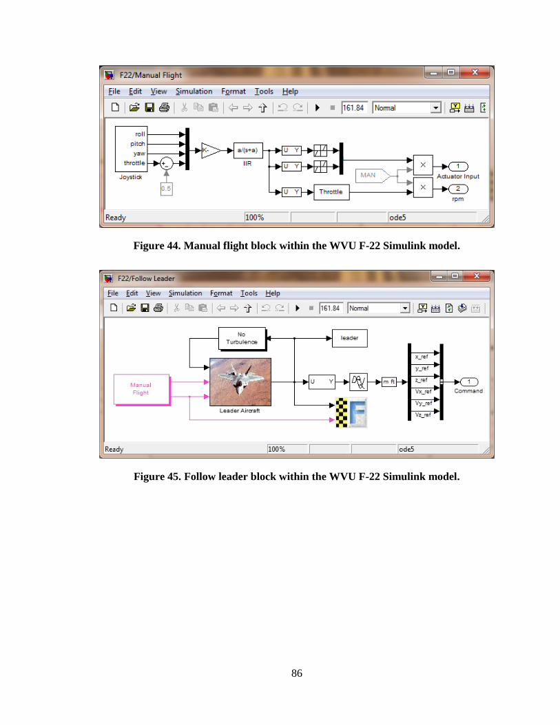
86

Figure 44. Manual flight block within the WVU F-22 Simulink model.

Figure 45. Follow leader block within the WVU F-22 Simulink model.

87

The following is the "SetColor.m" script for the WVU F-22 Simulink model:

% -------- Trajectory Generating Algorithms -------- set_param('F22/Disabled','ForegroundColor','red'); set_param('F22/Follow Leader','ForegroundColor','red'); set_param('F22/Follow Trajectory','ForegroundColor','red'); set_param('F22/Follow Trajectory/Voronoi TP','ForegroundColor','red'); set_param('F22/Follow Trajectory/Grid TP','ForegroundColor','red'); set_param('F22/Follow Trajectory/POI Simple

TP','ForegroundColor','red'); set_param('F22/Follow Trajectory/POI Advanced

TP','ForegroundColor','red'); set_param('F22/Follow Trajectory/Potential Field

TP','ForegroundColor','red'); set_param('F22/Follow Trajectory/Load

Trajectory','ForegroundColor','red'); set_param('F22/Follow Trajectory/POI V1','ForegroundColor','red'); set_param('F22/Follow Trajectory/POI V2','ForegroundColor','red'); set_param('F22/Follow Trajectory/Landing','ForegroundColor','red'); switch TrPlanAlg case 0 set_param('F22/Disabled','ForegroundColor','darkgreen'); case 1 set_param('F22/Follow

Trajectory','ForegroundColor','darkgreen'); set_param('F22/Follow Trajectory/Voronoi

TP','ForegroundColor','darkgreen'); case 2 set_param('F22/Follow

Trajectory','ForegroundColor','darkgreen'); set_param('F22/Follow Trajectory/Grid

TP','ForegroundColor','darkgreen'); case 3 set_param('F22/Follow

Trajectory','ForegroundColor','darkgreen'); set_param('F22/Follow Trajectory/POI Simple

TP','ForegroundColor','darkgreen'); case 4 set_param('F22/Follow

Trajectory','ForegroundColor','darkgreen'); set_param('F22/Follow Trajectory/POI Advanced

TP','ForegroundColor','darkgreen'); case 5 set_param('F22/Follow

Trajectory','ForegroundColor','darkgreen'); set_param('F22/Follow Trajectory/Potential Field

TP','ForegroundColor','darkgreen'); case 6 set_param('F22/Follow

Trajectory','ForegroundColor','darkgreen'); set_param('F22/Follow Trajectory/POI

V1','ForegroundColor','darkgreen'); case 7 set_param('F22/Follow

Trajectory','ForegroundColor','darkgreen');

88

set_param('F22/Follow Trajectory/POI

V2','ForegroundColor','darkgreen'); case 8 set_param('F22/Follow

Trajectory','ForegroundColor','darkgreen'); set_param('F22/Follow Trajectory/Load

Trajectory','ForegroundColor','darkgreen'); case 9 set_param('F22/Follow Leader','ForegroundColor','darkgreen'); end if Autoland == 1, set_param('F22/Follow

Trajectory/Landing','ForegroundColor','darkgreen'); end % --------------------------------------------------

% --------- Trajectory Tracking Algorithms --------- set_param('F22/Manual Flight','ForegroundColor','magenta'); set_param('F22/Conventional Controllers','ForegroundColor','magenta'); set_param('F22/Conventional Controllers/PID

Controller','ForegroundColor','magenta'); set_param('F22/Conventional Controllers/Virtual PID

Controller','ForegroundColor','magenta'); set_param('F22/Conventional Controllers/NLDI Outer

Controller','ForegroundColor','magenta'); set_param('F22/Conventional Controllers/NLDI Controller

Extended','ForegroundColor','magenta'); set_param('F22/Conventional Controllers/LQR

Controller','ForegroundColor','magenta'); set_param('F22/Adaptive Controllers','ForegroundColor','magenta'); set_param('F22/Adaptive Controllers/PID

Controller','ForegroundColor','magenta'); set_param('F22/Adaptive Controllers/Virtual PID

Controller','ForegroundColor','magenta'); set_param('F22/Adaptive Controllers/NLDI

Controller','ForegroundColor','magenta'); set_param('F22/Adaptive Controllers/NLDI Controller

Extended','ForegroundColor','magenta'); if ManualFlight == 1, set_param('F22/Manual Flight','ForegroundColor','darkgreen'); else switch TrTrackAlg case 1 set_param('F22/Conventional

Controllers','ForegroundColor','darkgreen'); set_param('F22/Conventional Controllers/PID

Controller','ForegroundColor','darkgreen'); case 2 set_param('F22/Conventional

Controllers','ForegroundColor','darkgreen'); set_param('F22/Conventional Controllers/Virtual PID

Controller','ForegroundColor','darkgreen'); case 3 set_param('F22/Conventional

Controllers','ForegroundColor','darkgreen');

89

set_param('F22/Conventional Controllers/NLDI Outer

Controller','ForegroundColor','darkgreen'); case 4 set_param('F22/Conventional

Controllers','ForegroundColor','darkgreen'); set_param('F22/Conventional Controllers/NLDI Controller

Extended','ForegroundColor','darkgreen'); case 5 set_param('F22/Conventional

Controllers','ForegroundColor','darkgreen'); set_param('F22/Conventional Controllers/LQR

Controller','ForegroundColor','darkgreen'); case 6 set_param('F22/Adaptive

Controllers','ForegroundColor','darkgreen'); set_param('F22/Adaptive Controllers/PID

Controller','ForegroundColor','darkgreen'); case 7 set_param('F22/Adaptive

Controllers','ForegroundColor','darkgreen'); set_param('F22/Adaptive Controllers/Virtual PID

Controller','ForegroundColor','darkgreen'); case 8 set_param('F22/Adaptive

Controllers','ForegroundColor','darkgreen'); set_param('F22/Adaptive Controllers/NLDI

Controller','ForegroundColor','darkgreen'); case 9 set_param('F22/Adaptive

Controllers','ForegroundColor','darkgreen'); set_param('F22/Adaptive Controllers/NLDI Controller

Extended','ForegroundColor','darkgreen'); end end % --------------------------------------------------

% ------------------ Other Blocks ------------------ if RealTime ==0, set_param('F22/Set Pace', 'ForegroundColor',

'red','MaskDisplay','disp(''Accelerated\nTime'')'); else set_param('F22/Set Pace', 'ForegroundColor',

'blue','MaskDisplay','disp(''Real Time'')'); end TurbulenceSeverity = 0; set_param('F22/Wind &

Turbulence','ForegroundColor','black','MaskDisplay','disp(''No\nTurbule

nce'')'); set_param('F22/Follow Leader/Wind &

Turbulence','ForegroundColor','black','MaskDisplay','disp(''No\nTurbule

nce'')'); % --------------------------------------------------

90

Figure 46. Aerodynamic forces computation within the Pioneer Simulink model.

91

Figure 47. Data manager block within the WVU F-22 Simulink model.

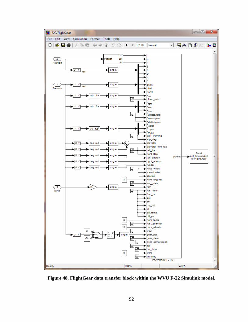
92

Figure 48. FlightGear data transfer block within the WVU F-22 Simulink model.

93

Figure 49. Dashboard data transfer block within the WVU F-22 Simulink model.

94

APPENDIX C

AIRCRAFT MODEL DESIGN CALCULATIONS

Thorough calculations have been carried out in order to obtain accurate new aircraft

modes. This appendix presents the required calculations to obtain stability and control

derivatives, as well as thrust profiles, for each newly implemented UAV model.

First, aircraft weight and moments of inertia had to be determined. This was done by

finding the CG positions of all items of known mass (engine, landing gear, fuel, and

payload) with respect to the CG of the aircraft. The rest of the UAV was treated as a set

of rectangles (wing, tail surfaces) and cylindrical objects (fuselage, booms) with uniform

mass distribution. An Excel spreadsheet, shown in Table 14 for the Pioneer, Table 15 for

the TigerShark, and Table 16 for the OX UAVs was then used to calculate the moments

of inertia about the aircraft CG. Moments of inertia were also estimated using quick

reference formulae for ballpark verification. Experimentally obtained moments of inertia

were available for the Pioneer UAV only. Table 17 shows the comparison between the

various methods used to calculate moments of inertia. Note that experimental values were

used for the Pioneer, and calculated values were used for TigerShark and OX flight

dynamics models.

Next, AVL was used to determine aircraft stability and control derivatives. This was done

using text input files shown below. The results obtained from AVL analysis are shown in

Table 5 and Table 7 in sections 4.3.4 and 4.4.3 respectively.

Finally, the OX UAV has a re-designed engine model. The corresponding maximum

thrust and idle thrust profiles are shown in Table 18 and, graphically, in Figure 50.

Table 14. Pioneer UAV moments of inertia calculation.

Pioneer Component About Component CG Distance From A/C CG About Aircraft CG

Re

ctan

gula

r O

bje

ct

Component Mass Chord Span Thickness Ixx Iyy Izz X Y Z Ixx Iyy Izz

Quantity lbs ft ft % kg-m2 kg-m2 kg-m2 ft ft ft kg-m2 kg-m2 kg-m2

Wing 60 1.8 16.9 15% 60.19 0.70 60.86 0.4 0 0.25 60.35 1.26 61.27 1

H-Tail 15 1.5 5.9 12% 1.84 0.12 1.95 7.2 0 0.25 1.87 32.93 34.72 1

V-Tail 5 1.5 2.1 12% 0.08 0.12 0.04 7.2 2.95 0.5 1.96 11.09 12.80 2

Cyl

ind

rica

l Ob

ject

Component Mass Length Diameter

- About Component CG Distance From A/C CG About Aircraft CG

Quantity lbs ft ft kg-m2 kg-m2 kg-m2 ft ft ft kg-m2 kg-m2 kg-m2

Fuselage 73 9.5 1.5 - 1.73 23.14 23.14 1.5 0 0 1.73 30.06 30.06 1

Boom 5 7.9 0.2 - 0.00 1.10 1.10 3.6 2.95 0 1.84 3.83 5.66 2

Po

int

Mas

s

Component Mass

- - - About Component CG Distance From A/C CG About Aircraft CG

Quantity lbs kg-m2 kg-m2 kg-m2 ft ft ft kg-m2 kg-m2 kg-m2

Engine 120 - - - 0 0 0 3.3 0 0 0.00 55.07 55.07 1

Main Gear 8 - - - 0 0 0 0.5 3.5 2 5.48 1.43 4.21 2

Nose Gear 6 - - - 0 0 0 4.8 0 2 1.01 6.84 5.83 1

Fuel 60 - - - 0 0 0 0 0 0 0.00 0.00 0.00 1

Payload 100 - - - 0 0 0 1.65 0 0 0.00 11.47 11.47 1

Total Weight: 452

Total Moments

Ixx Iyy Izz

kg-m2 kg-m3 kg-m4

83.52 170.33 243.75

Table 15. TigerShark UAV moments of inertia calculation.

TigerShark Component About Component CG Distance From A/C CG About Aircraft CG

Re

ctan

gula

r O

bje

ct

Component Mass Chord Span Thickness Ixx Iyy Izz X Y Z Ixx Iyy Izz

Quantity lbs ft ft % kg-m2 kg-m2 kg-m2 ft ft ft kg-m2 kg-m2 kg-m2

Wing 50 2.3 17.5 15% 53.79 0.95 54.70 0.35 0 0.4 54.13 1.54 54.96 1

H-Tail 10 1.5 4.4 12% 0.68 0.08 0.76 7.25 0 0 0.68 22.23 22.91 1

V-Tail 3 1.5 2.2 12% 0.05 0.07 0.02 7.25 2.2 0.4 0.68 6.74 7.28 2

Cyl

ind

rica

l Ob

ject

Component Mass Length Diameter

- About Component CG Distance From A/C CG About Aircraft CG

Quantity lbs ft ft kg-m2 kg-m2 kg-m2 ft ft ft kg-m2 kg-m2 kg-m2

Fuselage 52 7.6 1.2 - 0.79 10.55 10.55 1 0 0 0.79 12.74 12.74 1

Boom 5 8.2 0.2 - 0.00 1.18 1.18 3.3 2.2 0 1.02 3.48 4.49 2

Po

int

Mas

s

Component Mass

- - - About Component CG Distance From A/C CG About Aircraft CG

Quantity lbs kg-m2 kg-m2 kg-m2 ft ft ft kg-m2 kg-m2 kg-m2

Engine 80 - - - 0 0 0 2.3 0 0.2 0.13 17.97 17.83 1

Main Gear 6 - - - 0 0 0 0.5 3.5 2 4.11 1.07 3.16 2

Nose Gear 4 - - - 0 0 0 3.3 0 2 0.67 2.51 1.84 1

Fuel 78 - - - 0 0 0 0 0 0 0.00 0.00 0.00 1

Payload 30 - - - 0 0 0 1 0 0 0.00 1.26 1.26 1

Total Weight: 318

Total Moments

Ixx Iyy Izz

kg-m2 kg-m2 kg-m2

68.04 80.84 141.41

Table 16. OX UAV moments of inertia calculation.

OX Component About Component CG Distance From A/C CG About Aircraft CG

Re

ctan

gula

r O

bje

ct

Component Mass Chord Span Thickness Ixx Iyy Izz X Y Z Ixx Iyy Izz

Quantity lbs ft ft % kg-m2 kg-m2 kg-m2 ft ft ft kg-m2 kg-m2 kg-m2

Wing 22 1.5 15.0 15% 17.39 0.18 17.56 -0.375 0 0 17.39 0.31 17.69 1

V-Tail 2.5 1 2.44 15% 0.05 0.03 0.04 3.71 1 0.7 0.21 1.53 1.60 2

Cyl

ind

rica

l Ob

ject

Component Mass Length Diameter

- About Component CG Distance From A/C CG About Aircraft CG

Quantity lbs ft ft kg-m2 kg-m2 kg-m2 ft ft ft kg-m2 kg-m2 kg-m2

Fuselage 11 7.6 1.2 - 0.17 2.23 2.23 1 0 0 0.17 2.69 2.69 1

Boom 3 5.0 0.1 - 0.00 0.26 0.26 3.3 2 0 0.51 1.64 2.15 2

Po

int

Mas

s

Component Mass

- - - About Component CG Distance From A/C CG About Aircraft CG

Quantity lbs kg-m2 kg-m2 kg-m2 ft ft ft kg-m2 kg-m2 kg-m2

Engine 10 - - - 0 0 0 1.2 0 0.2 0.02 0.62 0.61 1

Main Gear 2 - - - 0 0 0 0.63 1.29 1.35 0.29 0.19 0.17 2

Nose Gear 2 - - - 0 0 0 2.35 0 1.35 0.15 0.62 0.47 1

Fuel 40 - - - 0 0 0 0 0 0 0.00 0.00 0.00 1

Payload 10 - - - 0 0 0 2 0 0 0.00 1.69 1.69 1

Total Weight: 110

Total Moments

Ixx Iyy Izz

kg-m2 kg-m2 kg-m2

19.74 12.64 30.98

98

Table 17. Moments of inertia comparison.

Comparison

Moments Of Inertia

Ixx Iyy Izz

kg-m2 kg-m3 kg-m4

Pio

nee

r

Estimated 69.04 109.37 140.12

Calculated 83.52 170.33 243.75

Experimental 47.23 90.95 111.48

% Difference 43% 47% 54%

Tige

rSh

ark Estimated 52.08 71.55 99.22

Calculated 68.04 80.84 141.41

% Difference 31% 13% 43%

OX

Estimated 13.24 8.16 18.48

Calculated 19.74 12.64 30.98

% Difference 49% 55% 68%

99

The following AVL input text file was used to provide geometry characteristics of the

Pioneer UAV, in order to carry out an AVL analysis.

Pioneer UAV

#=================================================

#Mach

0.1

#IYsym IZsym Zsym

0 0 0.0

#Sref Cref Bref

30.42 1.8 16.9

#Xref Yref Zref

0.0 0.0 0.0

#=================================================

SURFACE

Wing

#Nchord Cspace [ Nspan Sspace ]

10 1.0

YDUPLICATE

0.0

SCALE

1.0 1.0 1.0

TRANSLATE

0.0 0.0 0.0

ANGLE

0.0

SECTION

#Xle Yle Zle Chord Ainc Nspanwise Sspace

-0.66 0.0 0.25 1.8 0.0 10 0

NACA

4415

SECTION

#Xle Yle Zle Chord Ainc Nspanwise Sspace

-0.66 6.0 0.25 1.8 0.0 10 0

NACA

4415

CONTROL

#label gain Xhinge Xhvec Yhvec Zhvec SgnDup

Aileron -1.0 0.70 0.0 0.0 0.0 -1

SECTION

#Xle Yle Zle Chord Ainc Nspanwise Sspace

-0.66 8.0 0.25 1.8 0.0 10 0

NACA

100

4415

CONTROL

#label gain Xhinge Xhvec Yhvec Zhvec SgnDup

Aileron -1.0 0.70 0.0 0.0 0.0 -1

SECTION

#Xle Yle Zle Chord Ainc Nspanwise Sspace

-0.66 8.45 0.25 1.8 0.0 10 0

NACA

4415

#=================================================

SURFACE

Horizontal Tail

#Nchord Cspace [ Nspan Sspace ]

10 1.0

YDUPLICATE

0.0

SCALE

1.0 1.0 1.0

TRANSLATE

0.0 0.0 0.0

ANGLE

0.0

SECTION

#Xle Yle Zle Chord Ainc Nspanwise Sspace

6.97 0.0 0.25 1.0 0.0 10 0

NACA

0012

CONTROL

#label gain Xhinge Xhvec Yhvec Zhvec SgnDup

Elevator -0.95 0.66 0.0 0.0 0.0 1

SECTION

#Xle Yle Zle Chord Ainc Nspanwise Sspace

6.97 2.94 0.25 1.0 0.0 10 0

NACA

0012

CONTROL

#label gain Xhinge Xhvec Yhvec Zhvec SgnDup

Elevator -0.95 0.66 0.0 0.0 0.0 1

#=================================================

SURFACE

Vertical Tail

#Nchord Cspace [ Nspan Sspace ]

10 1.0

101

YDUPLICATE

0.0

SCALE

1.0 1.0 1.0

TRANSLATE

0.0 0.0 0.0

ANGLE

0.0

SECTION

#Xle Yle Zle Chord Ainc Nspanwise Sspace

6.97 2.94 -0.54 1.0 0.0 10 0

NACA

0012

CONTROL

#label gain Xhinge Xhvec Yhvec Zhvec SgnDup

Rudder -0.90 0.65 0.0 0.0 0.0 1

SECTION

#Xle Yle Zle Chord Ainc Nspanwise Sspace

6.97 2.94 1.53 1.0 0.0 10 0

NACA

0012

CONTROL

#label gain Xhinge Xhvec Yhvec Zhvec SgnDup

Rudder -0.90 0.65 0.0 0.0 0.0 1

#=================================================

SURFACE

Booms Horizontal

#Nchord Cspace [ Nspan Sspace ]

10 1.0

YDUPLICATE

0.0

SCALE

1.0 1.0 1.0

TRANSLATE

0.0 0.0 0.0

ANGLE

0.0

SECTION

#Xle Yle Zle Chord Ainc Nspanwise Sspace

0.0 1.4 0.25 7.9 0.0 1 0

NACA

0012

SECTION

#Xle Yle Zle Chord Ainc Nspanwise Sspace

102

0.0 1.6 0.25 7.9 0.0 1 0

NACA

0012

#=================================================

SURFACE

Booms Vertical

#Nchord Cspace [ Nspan Sspace ]

10 1.0

YDUPLICATE

0.0

SCALE

1.0 1.0 1.0

TRANSLATE

0.0 0.0 0.0

ANGLE

0.0

SECTION

#Xle Yle Zle Chord Ainc Nspanwise Sspace

0.0 1.5 0.15 7.5 0.0 1 0

NACA

0012

SECTION

#Xle Yle Zle Chord Ainc Nspanwise Sspace

0.0 1.5 0.35 7.5 0.0 1 0

NACA

0012

#=================================================

SURFACE

Fuselage Horizontal

#Nchord Cspace [ Nspan Sspace ]

20 1.0

YDUPLICATE

0.0

SCALE

1.0 1.0 1.0

TRANSLATE

0.0 0.0 0.0

ANGLE

0.0

SECTION

#Xle Yle Zle Chord Ainc Nspanwise Sspace

-6.1 0.0 -0.5 7.5 0.0 1 0

103

NACA

0012

SECTION

#Xle Yle Zle Chord Ainc Nspanwise Sspace

-5.4 0.4 -0.5 6.55 0.0 1 0

NACA

0012

SECTION

#Xle Yle Zle Chord Ainc Nspanwise Sspace

-4.5 0.6 -0.5 5.3 0.0 1 0

NACA

0012

#=================================================

SURFACE

Fuselage Vertical

#Nchord Cspace [ Nspan Sspace ]

20 1.0

YDUPLICATE

0.0

SCALE

1.0 1.0 1.0

TRANSLATE

0.0 0.0 0.0

ANGLE

0.0

SECTION

#Xle Yle Zle Chord Ainc Nspanwise Sspace

-5.4 0.0 -0.9 6.2 0.0 1 0

NACA

0012

SECTION

#Xle Yle Zle Chord Ainc Nspanwise Sspace

-6.1 0.0 -0.5 7.5 0.0 1 0

NACA

0012

SECTION

#Xle Yle Zle Chord Ainc Nspanwise Sspace

-3.0 0.0 0.5 4.4 0.0 1 0

NACA

0012

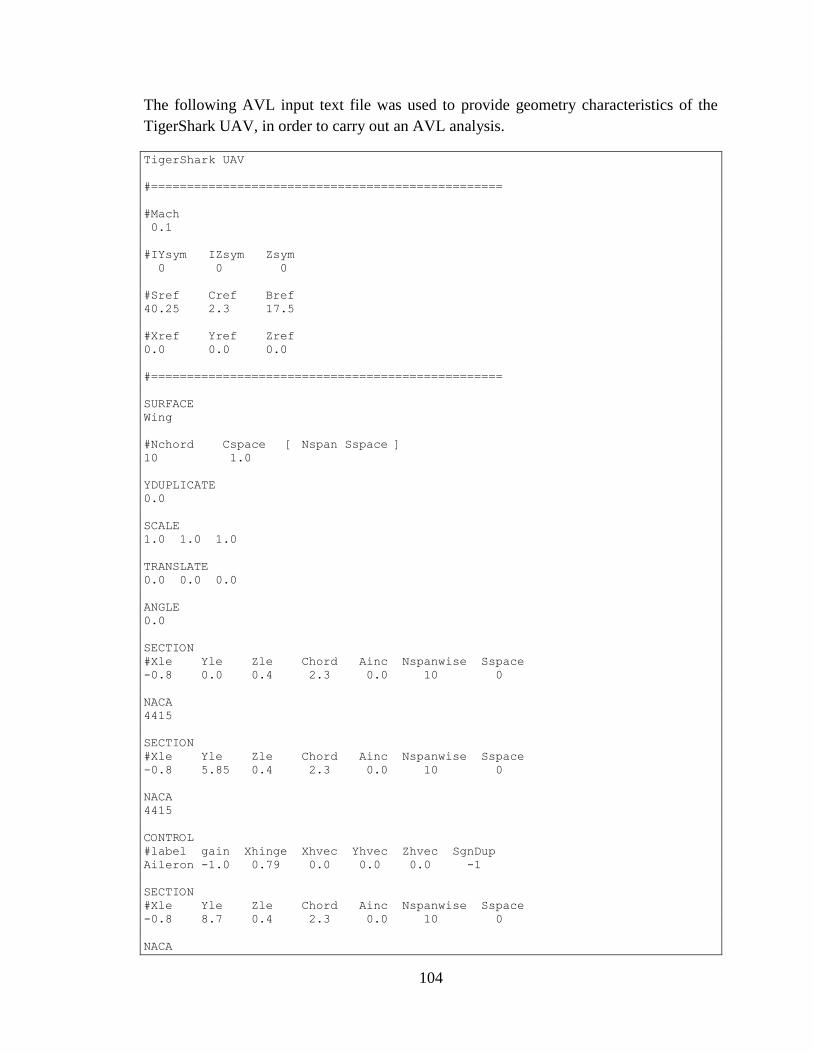
104

The following AVL input text file was used to provide geometry characteristics of the

TigerShark UAV, in order to carry out an AVL analysis.

TigerShark UAV

#=================================================

#Mach

0.1

#IYsym IZsym Zsym

0 0 0

#Sref Cref Bref

40.25 2.3 17.5

#Xref Yref Zref

0.0 0.0 0.0

#=================================================

SURFACE

Wing

#Nchord Cspace [ Nspan Sspace ]

10 1.0

YDUPLICATE

0.0

SCALE

1.0 1.0 1.0

TRANSLATE

0.0 0.0 0.0

ANGLE

0.0

SECTION

#Xle Yle Zle Chord Ainc Nspanwise Sspace

-0.8 0.0 0.4 2.3 0.0 10 0

NACA

4415

SECTION

#Xle Yle Zle Chord Ainc Nspanwise Sspace

-0.8 5.85 0.4 2.3 0.0 10 0

NACA

4415

CONTROL

#label gain Xhinge Xhvec Yhvec Zhvec SgnDup

Aileron -1.0 0.79 0.0 0.0 0.0 -1

SECTION

#Xle Yle Zle Chord Ainc Nspanwise Sspace

-0.8 8.7 0.4 2.3 0.0 10 0

NACA

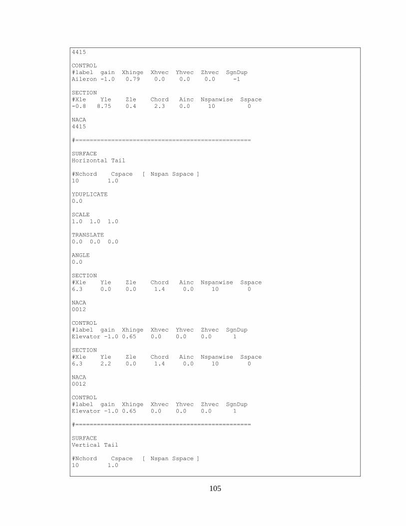
105

4415

CONTROL

#label gain Xhinge Xhvec Yhvec Zhvec SgnDup

Aileron -1.0 0.79 0.0 0.0 0.0 -1

SECTION

#Xle Yle Zle Chord Ainc Nspanwise Sspace

-0.8 8.75 0.4 2.3 0.0 10 0

NACA

4415

#=================================================

SURFACE

Horizontal Tail

#Nchord Cspace [ Nspan Sspace ]

10 1.0

YDUPLICATE

0.0

SCALE

1.0 1.0 1.0

TRANSLATE

0.0 0.0 0.0

ANGLE

0.0

SECTION

#Xle Yle Zle Chord Ainc Nspanwise Sspace

6.3 0.0 0.0 1.4 0.0 10 0

NACA

0012

CONTROL

#label gain Xhinge Xhvec Yhvec Zhvec SgnDup

Elevator -1.0 0.65 0.0 0.0 0.0 1

SECTION

#Xle Yle Zle Chord Ainc Nspanwise Sspace

6.3 2.2 0.0 1.4 0.0 10 0

NACA

0012

CONTROL

#label gain Xhinge Xhvec Yhvec Zhvec SgnDup

Elevator -1.0 0.65 0.0 0.0 0.0 1

#=================================================

SURFACE

Vertical Tail

#Nchord Cspace [ Nspan Sspace ]

10 1.0

106

YDUPLICATE

0.0

SCALE

1.0 1.0 1.0

TRANSLATE

0.0 0.0 0.0

ANGLE

0.0

SECTION

#Xle Yle Zle Chord Ainc Nspanwise Sspace

6.75 2.2 -0.4 0.95 0.0 10 0

NACA

0012

CONTROL

#label gain Xhinge Xhvec Yhvec Zhvec SgnDup

Rudder -0.90 0.63 0.0 0.0 0.0 1

SECTION

#Xle Yle Zle Chord Ainc Nspanwise Sspace

6.3 2.2 0.0 1.4 0.0 10 0

NACA

0012

CONTROL

#label gain Xhinge Xhvec Yhvec Zhvec SgnDup

Rudder -0.90 0.76 0.0 0.0 0.0 1

SECTION

#Xle Yle Zle Chord Ainc Nspanwise Sspace

6.75 2.2 1.3 0.95 0.0 10 0

NACA

0012

CONTROL

#label gain Xhinge Xhvec Yhvec Zhvec SgnDup

Rudder -0.90 0.63 0.0 0.0 0.0 1

#=================================================

SURFACE

Booms Horizontal

#Nchord Cspace [ Nspan Sspace ]

10 1.0

YDUPLICATE

0.0

SCALE

1.0 1.0 1.0

TRANSLATE

0.0 0.0 0.0

ANGLE

107

0.0

SECTION

#Xle Yle Zle Chord Ainc Nspanwise Sspace

-0.8 2.1 0.0 8.2 0.0 1 0

NACA

0012

SECTION

#Xle Yle Zle Chord Ainc Nspanwise Sspace

-0.8 2.3 0.0 8.2 0.0 1 0

NACA

0012

#=================================================

SURFACE

Booms Vertical

#Nchord Cspace [ Nspan Sspace ]

10 1.0

YDUPLICATE

0.0

SCALE

1.0 1.0 1.0

TRANSLATE

0.0 0.0 0.0

ANGLE

0.0

SECTION

#Xle Yle Zle Chord Ainc Nspanwise Sspace

-0.8 2.2 -0.1 8.2 0.0 1 0

NACA

0012

SECTION

#Xle Yle Zle Chord Ainc Nspanwise Sspace

-0.8 2.2 0.1 8.2 0.0 1 0

NACA

0012

#=================================================

SURFACE

Fuselage Horizontal

#Nchord Cspace [ Nspan Sspace ]

20 1.0

YDUPLICATE

0.0

SCALE

1.0 1.0 1.0

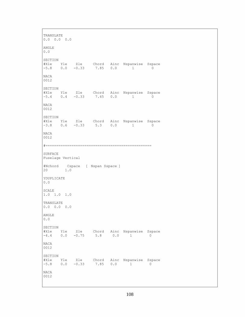
108

TRANSLATE

0.0 0.0 0.0

ANGLE

0.0

SECTION

#Xle Yle Zle Chord Ainc Nspanwise Sspace

-5.8 0.0 -0.33 7.85 0.0 1 0

NACA

0012

SECTION

#Xle Yle Zle Chord Ainc Nspanwise Sspace

-5.4 0.4 -0.33 7.45 0.0 1 0

NACA

0012

SECTION

#Xle Yle Zle Chord Ainc Nspanwise Sspace

-3.8 0.6 -0.33 5.3 0.0 1 0

NACA

0012

#=================================================

SURFACE

Fuselage Vertical

#Nchord Cspace [ Nspan Sspace ]

20 1.0

YDUPLICATE

0.0

SCALE

1.0 1.0 1.0

TRANSLATE

0.0 0.0 0.0

ANGLE

0.0

SECTION

#Xle Yle Zle Chord Ainc Nspanwise Sspace

-4.4 0.0 -0.75 5.8 0.0 1 0

NACA

0012

SECTION

#Xle Yle Zle Chord Ainc Nspanwise Sspace

-5.8 0.0 -0.33 7.85 0.0 1 0

NACA

0012

109

SECTION

#Xle Yle Zle Chord Ainc Nspanwise Sspace

-0.8 0.0 0.65 2.85 0.0 1 0

NACA

0012

110

The following AVL input text file was used to provide geometry characteristics of the

OX UAV, in order to carry out an AVL analysis.

OX UAV

#=================================================

#Mach

0.06

#IYsym IZsym Zsym

0 0 0

#Sref Cref Bref

24 1.5 15.0

#Xref Yref Zref

0.0 0.0 0.0

#=================================================

SURFACE

Wing

#Nchord Cspace [ Nspan Sspace ]

10 1.0

YDUPLICATE

0.0

SCALE

1.0 1.0 1.0

TRANSLATE

0.0 0.0 0.0

ANGLE

0.0

SECTION

#Xle Yle Zle Chord Ainc Nspanwise Sspace

-0.5 0.0 0.0 1.5 2.0 20 0

AFIL

n63415.dat

SECTION

#Xle Yle Zle Chord Ainc Nspanwise Sspace

-0.5 3.67 0.0 1.5 2.0 10 0

AFIL

n63415.dat

#CONTROL

#label gain Xhinge Xhvec Yhvec Zhvec SgnDup

#AileronIB -1.0 0.80 0.0 0.0 0.0 -1

SECTION

#Xle Yle Zle Chord Ainc Nspanwise Sspace

-0.5 5.58 0.0 1.5 2.0 10 0

AFIL

111

n63415.dat

#CONTROL

#label gain Xhinge Xhvec Yhvec Zhvec SgnDup

#AileronIB -1.0 0.80 0.0 0.0 0.0 -1

CONTROL

#label gain Xhinge Xhvec Yhvec Zhvec SgnDup

AileronOB -1.0 0.80 0.0 0.0 0.0 -1

SECTION

#Xle Yle Zle Chord Ainc Nspanwise Sspace

-0.5 7.45 0.0 1.5 2.0 10 0

AFIL

n63415.dat

CONTROL

#label gain Xhinge Xhvec Yhvec Zhvec SgnDup

AileronOB -1.0 0.80 0.0 0.0 0.0 -1

SECTION

#Xle Yle Zle Chord Ainc Nspanwise Sspace

-0.5 7.5 0.0 1.5 2.0 5 0

AFIL

n63415.dat

#=================================================

SURFACE

Inverted V-Tail

#Nchord Cspace [ Nspan Sspace ]

10 1.0

YDUPLICATE

0.0

SCALE

1.0 1.0 1.0

TRANSLATE

0.0 0.0 0.0

ANGLE

0.0

SECTION

#Xle Yle Zle Chord Ainc Nspanwise Sspace

3.69 2.0 0.0 1.0 0.0 10 0

AFIL

n63415.dat

CONTROL

#label gain Xhinge Xhvec Yhvec Zhvec SgnDup

Elevator -1.0 0.70 0.0 0.0 0.0 1

CONTROL

#label gain Xhinge Xhvec Yhvec Zhvec SgnDup

Ruddervator -1.0 0.70 0.0 0.0 0.0 -1

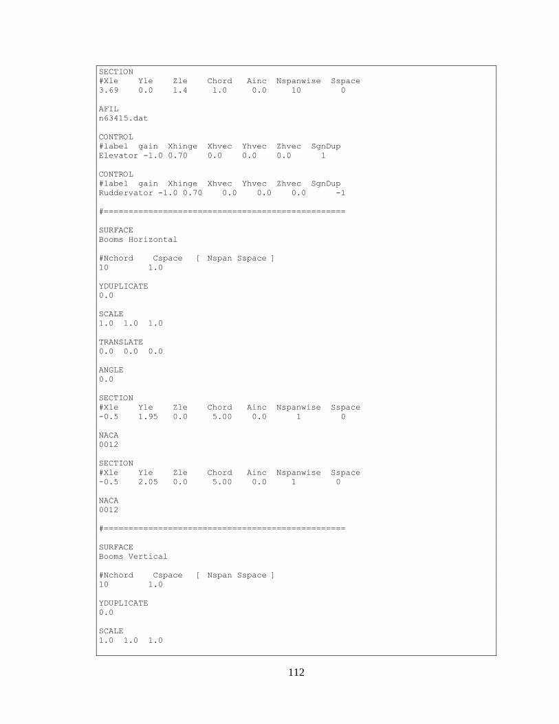
112

SECTION

#Xle Yle Zle Chord Ainc Nspanwise Sspace

3.69 0.0 1.4 1.0 0.0 10 0

AFIL

n63415.dat

CONTROL

#label gain Xhinge Xhvec Yhvec Zhvec SgnDup

Elevator -1.0 0.70 0.0 0.0 0.0 1

CONTROL

#label gain Xhinge Xhvec Yhvec Zhvec SgnDup

Ruddervator -1.0 0.70 0.0 0.0 0.0 -1

#=================================================

SURFACE

Booms Horizontal

#Nchord Cspace [ Nspan Sspace ]

10 1.0

YDUPLICATE

0.0

SCALE

1.0 1.0 1.0

TRANSLATE

0.0 0.0 0.0

ANGLE

0.0

SECTION

#Xle Yle Zle Chord Ainc Nspanwise Sspace

-0.5 1.95 0.0 5.00 0.0 1 0

NACA

0012

SECTION

#Xle Yle Zle Chord Ainc Nspanwise Sspace

-0.5 2.05 0.0 5.00 0.0 1 0

NACA

0012

#=================================================

SURFACE

Booms Vertical

#Nchord Cspace [ Nspan Sspace ]

10 1.0

YDUPLICATE

0.0

SCALE

1.0 1.0 1.0

113

TRANSLATE

0.0 0.0 0.0

ANGLE

0.0

SECTION

#Xle Yle Zle Chord Ainc Nspanwise Sspace

-0.5 2.0 -0.05 5.00 0.0 1 0

NACA

0012

SECTION

#Xle Yle Zle Chord Ainc Nspanwise Sspace

-0.5 2.0 0.05 5.00 0.0 1 0

NACA

0012

#=================================================

SURFACE

Fuselage Horizontal

#Nchord Cspace [ Nspan Sspace ]

20 1.0

YDUPLICATE

0.0

SCALE

1.0 1.0 1.0

TRANSLATE

0.0 0.0 0.0

ANGLE

0.0

SECTION

#Xle Yle Zle Chord Ainc Nspanwise Sspace

-3.05 0.0 -0.05 4.10 0.0 1 0

NACA

0012

SECTION

#Xle Yle Zle Chord Ainc Nspanwise Sspace

-3.05 0.3 -0.05 4.10 0.0 1 0

NACA

0012

SECTION

#Xle Yle Zle Chord Ainc Nspanwise Sspace

-2.75 0.5 -0.05 3.80 0.0 1 0

NACA

0012

#=================================================

114

SURFACE

Fuselage Vertical

#Nchord Cspace [ Nspan Sspace ]

20 1.0

YDUPLICATE

0.0

SCALE

1.0 1.0 1.0

TRANSLATE

0.0 0.0 0.0

ANGLE

0.0

SECTION

#Xle Yle Zle Chord Ainc Nspanwise Sspace

-2.75 0.0 -0.42 3.80 0.0 1 0

NACA

0012

SECTION

#Xle Yle Zle Chord Ainc Nspanwise Sspace

-3.05 0.0 -0.05 4.10 0.0 1 0

NACA

0012

SECTION

#Xle Yle Zle Chord Ainc Nspanwise Sspace

-2.75 0.0 0.32 3.80 0.0 1 0

NACA

0012

The following run case

Run case 1: -Cruise-

alpha -> CL = 0.81000

beta -> beta = 0.00000

pb/2V -> pb/2V = 0.00000

qc/2V -> qc/2V = 0.00000

rb/2V -> rb/2V = 0.00000

AileronOB -> Cl roll mom = 0.00001

Elevator -> Cm pitchmom = 0.00001

Ruddervator -> Cn yaw mom = 0.00001

CDo = 0.06000

bank = 0.00000 deg

elevation = 0.00000 deg

heading = 0.00000 deg

Mach = 0.06000

velocity = 69.2000 Lunit/Tunit

density = 0.07647 Munit/Lunit^3

grav.acc. = 32.1850 Lunit/Tunit^2

115

turn_rad. = 0.00000 Lunit

load_fac. = 1.00000

X_cg = 0.00000 Lunit

Y_cg = 0.00000 Lunit

Z_cg = 0.00000 Lunit

mass = 110.000 Munit

Ixx = 468.490 Munit-Lunit^2

Iyy = 299.970 Munit-Lunit^2

Izz = 735.100 Munit-Lunit^2

Ixy = 0.00000 Munit-Lunit^2

Iyz = 0.00000 Munit-Lunit^2

Izx = 0.00000 Munit-Lunit^2

visc CL_a = 0.00000

visc CL_u = 0.00000

visc CM_a = 0.00000

visc CM_u = 0.00000

116

Table 18. OX UAV thrust profile.

Velocity [knots]

Max RPM Max Thrust

[N] Idle Thrust

[N]

0 6000 150 53

2 6058 180 53

4 6117 200 53

6 6175 215 53

8 6234 220 53

10 6292 225 53

12 6351 227 53

14 6409 227 53

16 6468 221 53

18 6526 216 53

20 6585 211 53

22 6643 205 53

24 6702 200 53

26 6760 194 53

28 6818 189 52

30 6877 184 52

32 6935 178 51

34 6994 173 50

36 7052 168 48

38 7111 162 42

40 7169 157 37

42 7228 152 32

44 7286 146 26

46 7345 141 21

48 7403 136 16

50 7462 130 10

52 7520 125 5

54 7578 120 0

56 7637 114 -6

58 7695 109 -11

60 7754 104 -17

62 7812 98 -22

64 7871 93 -27

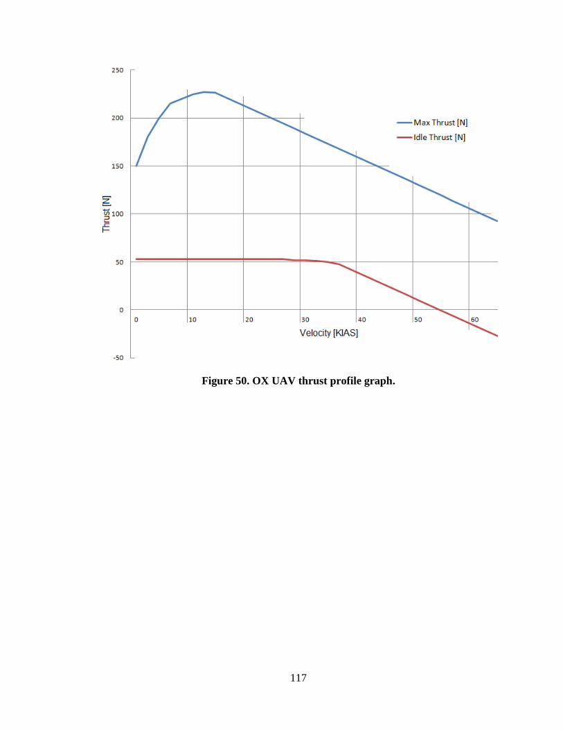
117

Figure 50. OX UAV thrust profile graph.