Two-sided Exact Tests and Matching Confidence Intervals ... · Motivating Example 1: Fisher’s...

Two-sided Exact Tests and Matching ConfidenceIntervals for Discrete Data

Michael P. Fay

National Institute of Allergy and Infectious Diseases

useR! 2010 ConferenceJuly 21, 2010

Motivating Example 1: Fisher’s exact Test for 2×2 Table

Homozygous for Wild Type or HeterozygousCCR5∆32 mutation for CCR5∆32 mutation

Abdominal Pain 4 (26.7%) 50 (8.1%)No Abdom. Pain 11 (73.3%) 569 (91.9%)

Relationship of CCR5∆32 mutation (genetic recessive model) toEarly Symptoms with West Nile Virus Infection(from Lim, et al, J Infectious Diseases, 2010, 178-185)

Analysis in R 2.11.1

Step 1: Create 2 by 2 Table

> abdpain<-matrix(c(4,50,11,569),2,2,

+ dimnames=list(c("Abdominal Pain","No Abdom. Pain"),

+ c("Homo","WT/Hetero")))

> abdpain

Homo WT/Hetero

Abdominal Pain 4 50

No Abdom. Pain 11 569

Analysis in R 2.11.1, stats package

Step 2: Run test

> fisher.test(abdpain)

Fisher's Exact Test for Count Data

data: abdpain

p-value = 0.03166

alternative hypothesis: true odds ratio is not equal to 1

95 percent confidence interval:

0.9235364 14.5759712

sample estimates:

odds ratio

4.122741

Test-CI Inconsistency

Problem: Test rejects but confidence intervalincludes odds ratio of 1.

I Same problem in:I R (fisher.test), Version 2.11.1,I SAS (Proc Freq), Version 9.2 andI StatXact, (StatXact 8 Procs).

I In all 3: One and only one exact confidence for odds ratio forthe 2 by 2 table is given, AND

I the confidence interval is not an inversion of the usualtwo-sided Fisher’s exact test.

I (Test defined the same way in all 3 programs).

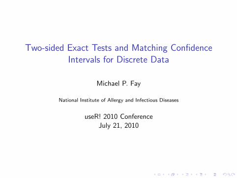
Example 2: One Sample Binomial Test

Observe 10 out of 100 from a simulation. Is this significantlydifferent from a true proportion of 0.05?

> binom.test(10,100,p=0.05)

Exact binomial test

data: 10 and 100

number of successes = 10, number of trials = 100, p-value = 0.03411

alternative hypothesis: true probability of success is not equal to 0.05


0.04900469 0.17622260

sample estimates:

probability of success

0.1

Example 3: Two Sample Poisson Test

If we observe rates 2/17887 (about 11.2 per 100,000) for thestandard treatment and 10/20000 ( 50 per 100,000) for newtreatment, do these two groups significantly differ by exact Poissonrate test?

> poisson.test(c(10,2),c(20000,17877))

Comparison of Poisson rates

data: c(10, 2) time base: c(20000, 17877)

count1 = 10, expected count1 = 6.336, p-value = 0.04213

alternative hypothesis: true rate ratio is not equal to 1


0.952422 41.950915

sample estimates:

rate ratio

4.46925

What is happening in the examples?

I In each example, we used an exact test and anexact confidence interval, but,

I the confidence interval is not an inversion ofthe test.

I Definition: confidence interval by inversionof (a series of) tests = all parameter valuesthat fail to reject point null hypothesis.

Definition: Inversion of Family of Tests

I Consider a series of tests, indexed by β0I Let x be data.

I Let pβ0(x) be p-value for testing the following hypotheses:

H0 : β = β0

H1 : β 6= β0

Then the inversion confidence set is

C (x, 1− α) = {β : pβ(x) > α}

Cannot have test-confidence set inconsistency with inversionconfidence set.

●●●●●●●●●●●●●●●●●●●●●●●●●●●●●●●●●●●●●●●●●●●●●●●●●●●●●●●●●●●●●●●●●●●●●●●●●●●●●●●●●●●●●●●●●●●●●●●●●●●●●●●●●●●●●●●●●●●●●●●●●●●●●●●●●●●●●●●●●●●●●●●●●●●●●●●●●●●●●●●●●●●●●●●●●●●●●●●●●●●●●●●●●●●●●●●●●●

●●●●●●●●●●●●●●●●●●●●●●●●●●●●●●●●●●●●●

●●●●●●●●●●●●●●●●●●●●●●●

●●●●●●●●●●●●●●●●●

●●●●●●●●●●●●●●

●●●●●●●●●●●●

●●●●●●●●●●

●●●●●●●●●

●●●●●●●●

●●●●●●●●

●●●●●●●●●●●●●●●●

●●●●●●●●●●●●●

●●●●●●●●●

●●●●●●●●

●●●●●●●●●●●●●●●●●●●●●●

●●●●●●●●●●●●●

●●●●●●●●●

●●●●●●●●

●●●●●●●●●

●●●●●●●●●●●●●●●●●●●

●●●●●●●●●●●●●

●●●●●●●●●●●●●●●●●●●●●●●●●●●●●●●●●●●●●●●●●●●●●●●●●●●●●●●

●●●●●●●●●●●●●●●●●●●●●●●●●

●●●●●●●●●●●●●●●●●●●●●●●●

●●●●●●●●●●●●●●●●●●●●●●●●

●●●●●●●●●●●●●●●●●●●●●●●

●●●●●●●●●●●●●●●●●●●●●●●

●●●●●●●●●●●●●●●●●●●●●●●●

●●●●●●●●●●●●●●●●●●●●●●●●●

●●●●●●●●●●●●●●●●●●●●●●●●●●●●●●●●●●●●●●●●●●●●●●●●●●●●●●●●●●●●●●●●●●●●●●●●●●●●●●●●●●●●●●●●●●●●●●●●●●●●●●●●●●●●●●●●●●●●●●●●●●●●●●●●●●●●●●●●●●●●●●●●●●●●●●●●●●●●●●●●●●●●●●●●●●●●●●

0.5 1.0 2.0 5.0 10.0 20.0

0.0

0.2

0.4

0.6

0.8

1.0

β0

two−

side

d p−

valu

e

● p= 0.032p= 0.032

Figure: CCR5 data: Abdominal Pain, usual two-sided Fisher’s exactp-values

●●●●●●●●●●●●●●●●●●●●●●●●●●●●●●●●●●●●●●●●●●●●●●●●●●●●●●●●●●●●●●●●●●●●●●●●●●●●●●●●●●●●●●●●●●●●●●●●●●●●●●●●●●●●●●●●●●●●●●●●●●●●●●●●●●●●●●●●●●●●●●●●●●●●●●●●●●●●●●●●●●●●●●●●●●●●●●●●●●●●●●●●●●●●●●●●●●

●●●●●●●●●●●●●●●●●●●●●●●●●●●●●●●●●●●●●

●●●●●●●●●●●●●●●●●●●●●●●

●●●●●●●●●●●●●●●●●

●●●●●●●●●●●●●●

●●●●●●●●●●●●

●●●●●●●●●●

●●●●●●●●●

●●●●●●●●

●●●●●●●●

●●●●●●●●●●●●●●●●

●●●●●●●●●●●●●

●●●●●●●●●

●●●●●●●●

●●●●●●●●●●●●●●●●●●●●●●

●●●●●●●●●●●●●

●●●●●●●●●

●●●●●●●●

●●●●●●●●●

●●●●●●●●●●●●●●●●●●●

●●●●●●●●●●●●●

●●●●●●●●●●●●●●●●●●●●●●●●●●●●●●●●●●●●●●●●●●●●●●●●●●●●●●●

●●●●●●●●●●●●●●●●●●●●●●●●●

●●●●●●●●●●●●●●●●●●●●●●●●

●●●●●●●●●●●●●●●●●●●●●●●●

●●●●●●●●●●●●●●●●●●●●●●●

●●●●●●●●●●●●●●●●●●●●●●●

●●●●●●●●●●●●●●●●●●●●●●●●

●●●●●●●●●●●●●●●●●●●●●●●●●

●●●●●●●●●●●●●●●●●●●●●●●●●●●●●●●●●●●●●●●●●●●●●●●●●●●●●●●●●●●●●●●●●●●●●●●●●●●●●●●●●●●●●●●●●●●●●●●●●●●●●●●●●●●●●●●●●●●●●●●●●●●●●●●●●●●●●●●●●●●●●●●●●●●●●●●●●●●●●●●●●●●●●●●●●●●●●●

0.5 1.0 2.0 5.0 10.0 20.0

0.0

0.2

0.4

0.6

0.8

1.0

β0

two−

side

d p−

valu

e

●

95 % CI=(1.17,14.2)95 % CI=(1.17,14.2)

Figure: CCR5 data: Abdominal Pain, 95 % inversion confidence intervalto usual two-sided Fisher’s exact

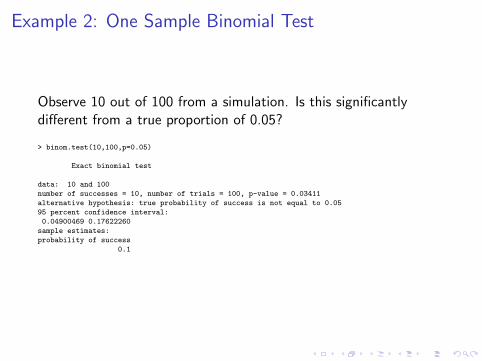
Another two-sided Fisher’s exact Test

I Define p-value as 2 times minimum of the one-sided Fisher’sexact p-values.

I Inversion of that two sided Fisher’s exact is the usual exactconfidence intervals.

I Call it Central Fisher’s exact Test

●●●●●●●●●●●●●●●●●●●●●●●●●●●●●●●●●●●●●●●●●●●●●●●●●●●●●●●●●●●●●●●●●●●●●●●●●●●●●●●●●●●●●●●●●●●●●●●●●●●●●●●●●●●●●●●●●●●●●●●●●●●●●●●●●●●●●●●●●●●●●●●●●●●●●●●●●●●●●●●●●●●●●●●●●●●●●●●●●●●●●●●●●●●●●●●●●●

●●●●●●●●●●●●●●●●●●●●●●●●●●●●●●●●●●●●●

●●●●●●●●●●●●●●●●●●●●●●●

●●●●●●●●●●●●●●●●●

●●●●●●●●●●●●●●

●●●●●●●●●●●●

●●●●●●●●●●

●●●●●●●●●

●●●●●●●●

●●●●●●●●

●●●●●●●●●●●●●●●●

●●●●●●●●●●●●●

●●●●●●●●●

●●●●●●●●

●●●●●●●●●●●●●●●●●●●●●●

●●●●●●●●●●●●●

●●●●●●●●●

●●●●●●●●

●●●●●●●●●

●●●●●●●●●●●●●●●●●●●

●●●●●●●●●●●●●

●●●●●●●●●●●●●●●●●●●●●●●●●●●●●●●●●●●●●●●●●●●●●●●●●●●●●●●

●●●●●●●●●●●●●●●●●●●●●●●●●

●●●●●●●●●●●●●●●●●●●●●●●●

●●●●●●●●●●●●●●●●●●●●●●●●

●●●●●●●●●●●●●●●●●●●●●●●

●●●●●●●●●●●●●●●●●●●●●●●

●●●●●●●●●●●●●●●●●●●●●●●●

●●●●●●●●●●●●●●●●●●●●●●●●●

●●●●●●●●●●●●●●●●●●●●●●●●●●●●●●●●●●●●●●●●●●●●●●●●●●●●●●●●●●●●●●●●●●●●●●●●●●●●●●●●●●●●●●●●●●●●●●●●●●●●●●●●●●●●●●●●●●●●●●●●●●●●●●●●●●●●●●●●●●●●●●●●●●●●●●●●●●●●●●●●●●●●●●●●●●●●●●

0.5 1.0 2.0 5.0 10.0 20.0

0.0

0.2

0.4

0.6

0.8

1.0

β0

two−

side

d p−

valu

e

Figure: CCR5 data: Abdominal Pain, gray= usual two-sided Fisher’sexact p-values, red=twice minimum one-sided p-values

●●●●●●●●●●●●●●●●●●●●●●●●●●●●●●●●●●●●●●●●●●●●●●●●●●●●●●●●●●●●●●●●●●●●●●●●●●●●●●●●●●●●●●●●●●●●●●●●●●●●●●●●●●●●●●●●●●●●●●●●●●●●●●●●●●●●●●●●●●●●●●●●●●●●●●●●●●●●●●●●●●●●●●●●●●●●●●●●●●●●●●●●●●●●●●●●●●

●●●●●●●●●●●●●●●●●●●●●●●●●●●●●●●●●●●●●

●●●●●●●●●●●●●●●●●●●●●●●

●●●●●●●●●●●●●●●●●

●●●●●●●●●●●●●●

●●●●●●●●●●●●

●●●●●●●●●●

●●●●●●●●●

●●●●●●●●

●●●●●●●●

●●●●●●●●●●●●●●●●

●●●●●●●●●●●●●

●●●●●●●●●

●●●●●●●●

●●●●●●●●●●●●●●●●●●●●●●

●●●●●●●●●●●●●

●●●●●●●●●

●●●●●●●●

●●●●●●●●●

●●●●●●●●●●●●●●●●●●●

●●●●●●●●●●●●●

●●●●●●●●●●●●●●●●●●●●●●●●●●●●●●●●●●●●●●●●●●●●●●●●●●●●●●●

●●●●●●●●●●●●●●●●●●●●●●●●●

●●●●●●●●●●●●●●●●●●●●●●●●

●●●●●●●●●●●●●●●●●●●●●●●●

●●●●●●●●●●●●●●●●●●●●●●●

●●●●●●●●●●●●●●●●●●●●●●●

●●●●●●●●●●●●●●●●●●●●●●●●

●●●●●●●●●●●●●●●●●●●●●●●●●

●●●●●●●●●●●●●●●●●●●●●●●●●●●●●●●●●●●●●●●●●●●●●●●●●●●●●●●●●●●●●●●●●●●●●●●●●●●●●●●●●●●●●●●●●●●●●●●●●●●●●●●●●●●●●●●●●●●●●●●●●●●●●●●●●●●●●●●●●●●●●●●●●●●●●●●●●●●●●●●●●●●●●●●●●●●●●●

0.5 1.0 2.0 5.0 10.0 20.0

0.0

0.2

0.4

0.6

0.8

1.0

β0

two−

side

d p−

valu

e

●

95 % central CI=(0.92,14.6)95 % central CI=(0.92,14.6)

twice one−sided p=0.063twice one−sided p=0.063

Figure: CCR5 data: Abdominal Pain, 95 % central confidence intervals

●●●●●●●●●●●●●●●●●●●●●●●●●●●●●●●●●●●●●●●●●●●●●●●●●●●●●●●●●●●●●●●●●●●●●●●●●●●●●●●●●●●●●●●●●●●●●●●●●●●●●●●●●●●●●●●●●●●●●●●●●●●●●●●●●●●●●●●●●●●●●●●●●●●●●●●●●●●●●●●●●●●●●●●●●●●●●●●●●●●●●●●●●●●●●●●●●●

●●●●●●●●●●●●●●●●●●●●●●●●●●●●●●●●●●●●●

●●●●●●●●●●●●●●●●●●●●●●●

●●●●●●●●●●●●●●●●●

●●●●●●●●●●●●●●

●●●●●●●●●●●●

●●●●●●●●●●

●●●●●●●●●

●●●●●●●●

●●●●●●●●

●●●●●●●●●●●●●●●●

●●●●●●●●●●●●●

●●●●●●●●●

●●●●●●●●

●●●●●●●●●●●●●●●●●●●●●●

●●●●●●●●●●●●●

●●●●●●●●●

●●●●●●●●

●●●●●●●●●

●●●●●●●●●●●●●●●●●●●

●●●●●●●●●●●●●

●●●●●●●●●●●●●●●●●●●●●●●●●●●●●●●●●●●●●●●●●●●●●●●●●●●●●●●

●●●●●●●●●●●●●●●●●●●●●●●●●

●●●●●●●●●●●●●●●●●●●●●●●●

●●●●●●●●●●●●●●●●●●●●●●●●

●●●●●●●●●●●●●●●●●●●●●●●

●●●●●●●●●●●●●●●●●●●●●●●

●●●●●●●●●●●●●●●●●●●●●●●●

●●●●●●●●●●●●●●●●●●●●●●●●●

●●●●●●●●●●●●●●●●●●●●●●●●●●●●●●●●●●●●●●●●●●●●●●●●●●●●●●●●●●●●●●●●●●●●●●●●●●●●●●●●●●●●●●●●●●●●●●●●●●●●●●●●●●●●●●●●●●●●●●●●●●●●●●●●●●●●●●●●●●●●●●●●●●●●●●●●●●●●●●●●●●●●●●●●●●●●●●

0.5 1.0 2.0 5.0 10.0 20.0

0.0

0.2

0.4

0.6

0.8

1.0

β0

two−

side

d p−

valu

e

●

95 % central CI=(0.92,14.6)95 % central CI=(0.92,14.6)

twice one−sided p=0.063twice one−sided p=0.063

●

95 % minlike CI=(1.17,14.2)95 % minlike CI=(1.17,14.2)

usual two−sided p=0.032usual two−sided p=0.032

Figure: CCR5 data: Abdominal Pain, 95 % central confidence intervals

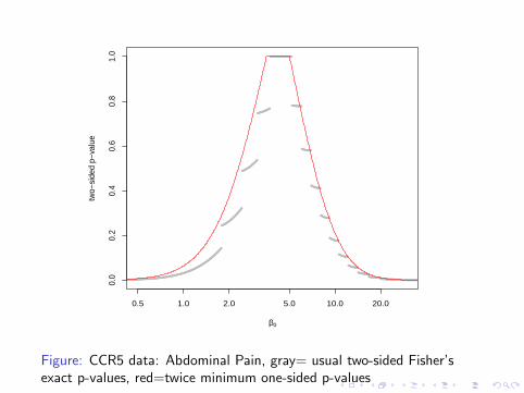
3 Ways to Calculate Two-sided p-values

central: 2 times minimum of one-sided p-values,

minlike: sum of probabilities of outcomes withlikelihoods less than or equal to observed.

pm(x) =∑

X :f (X )≤f (x)

f (X )

blaker: take smaller observed tail and add largestprobability on the opposite tail that doesnot exceed observed tail.

0 5 10 15

0.00

0.05

0.10

0.15

0.20

x=number of events in treatment group

nonc

entra

l hyp

erge

omet

ric d

ensi

ty

Pr[X<=4]= 0.0877 Pr[X>=10]= 0.0883

odds ratio= 10.55

two−sided p−value= 0.176(black+gray+green+blue)

central p−value= 0.1752*(black+gray)

two−sided p−value= 0.116(black+gray+blue)

Figure: CCR5 data: Abdominal Pain

Solution: Use “Matching” Confidence Intervals

Smallest confidence interval that contains all parameters that failto reject.

> library(exact2x2)

Loading required package: exactci

> fisher.exact(abdpain)

Two-sided Fisher's Exact Test (usual method using minimum likelihood)

data: abdpain

p-value = 0.03166



1.1734 14.1659

sample estimates:

odds ratio

4.122741


> fisher.exact(abdpain,tsmethod="central")

Central Fisher's Exact Test

data: abdpain

p-value = 0.06332



0.9235364 14.5759712

sample estimates:

odds ratio

4.122741


> blaker.exact(abdpain)

Blaker's Exact Test

data: abdpain

p-value = 0.03166



1.1734 14.2183

sample estimates:

odds ratio

4.122741

Example 2: One Sample Binomial

> library(exactci)

> binom.exact(10,100,p=0.05)

Exact two-sided binomial test (central method)

data: 10 and 100




0.04900469 0.17622260

sample estimates:


0.1


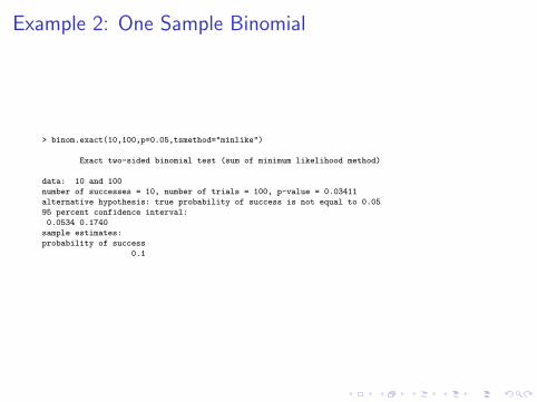
> binom.exact(10,100,p=0.05,tsmethod="minlike")

Exact two-sided binomial test (sum of minimum likelihood method)

data: 10 and 100




0.0534 0.1740

sample estimates:


0.1


> binom.exact(10,100,p=0.05,tsmethod="blaker")

Exact two-sided binomial test (Blaker's method)

data: 10 and 100




0.0513 0.1723

sample estimates:


0.1

Example 3: Two Sample Poisson

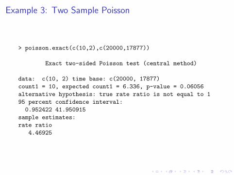
> poisson.exact(c(10,2),c(20000,17877))

Exact two-sided Poisson test (central method)

data: c(10, 2) time base: c(20000, 17877)




0.952422 41.950915

sample estimates:

rate ratio

4.46925


> poisson.exact(c(10,2),c(20000,17877),tsmethod="minlike")

Exact two-sided Poisson test (sum of minimum likelihood method)

data: c(10, 2) time base: c(20000, 17877)




1.061630 28.412707

sample estimates:

rate ratio

4.46925


> poisson.exact(c(10,2),c(20000,17877),tsmethod="blaker")

Exact two-sided Poisson test (Blaker's method)

data: c(10, 2) time base: c(20000, 17877)




1.068068 28.412707

sample estimates:

rate ratio

4.46925

An Anomaly: Unavoidable Test-CI Inconsistency

Made-Up Example:Group A Group B

Event 7 (2.67 %) 30 (6.07%)No Event 255 (97.33 %) 464 (93.93%)

I usual two-sided Fisher’s exact test p = 0.04996

I 95% inversion confidence set:

{β : β ∈ (0.177, 0.993) or β ∈ (1.006, 1.014)}

Matching CI defined as smallest interval that contains all elementsof inversion confidence set:

(0.177, 1.014)

Unavoidable test-CI inconsistency!

●●●●●●●●●●●●●●●●●●●●●●●●●●●●●●●●●●●●●●●●●●●●●●●●●●●●●●●●●●●●●●●●●●●●●●●●●●●●●●●●●●●●●●●●●●●●●●●●●●●●●●●●●●●●●●●●●●●●●●●●●●●●●●●●●●●●●●●●●●●●●●●●●●●●●●●●●●●●●●●●●●●●●●●●●●●●●●●●●●●●●●●●●●●●●●●●●●●●●●●●●●●●●●●●●●●●●●●●●●●●●●●●●●●●●●●●●●●●●●●●●●●●●●●●●●●●●●●●●●●●●●●●●●●●●●●●●●●●●●●●●●●●●●●●●●●●●●●●●●●●●●●●●●●●●●●●●●●●●●●●●●●●●●●●●●●●●●●●●●●●●●●●●●●●●●●●●●●●●●●●●●●●●●●●●●●●●●●●●●●●●●●●●●●●●●●●●●●●●●●●●●●●●●●●●●●●●●●●●●●●●●●●●●●●●●●●●●●●●●●●●●●●●●●●●●●●●●●●●●●●●●●●●●●●●●●●●●●●●●●●●●●●●●●●●●●●●●●●●●●●●●●●●●●●●●●●●●●●●●●●●●●●●●●●●●●●●●●●●●●●●●●●●●●●●●●●●●●●●●●●●●●●●●●●●●●●●●●●●●●●●●●●●●●●●●●●●●●●●●●●●●●●●●●●●●●●●●●●●●●●●

0.94 0.96 0.98 1.00 1.02

0.04

900.

0495

0.05

000.

0505

0.05

10

β0

two−

side

d p−

valu

e

Figure: Made-up example, gray=usual two-sided Fisher’s exact, blue=Blaker’s exact p-values, red=twice minimum one-sided p-values

References

I Fay (2010) Biostatistics 373-374

I Fay (2010) R Journal, 2(1): 53-58.

I R package: exact2x2I R package: exactci

Two-sided Exact Tests and Matching Confidence Intervals ... · Motivating Example 1: Fisher’s...

Documents

Transcript of Two-sided Exact Tests and Matching Confidence Intervals ... · Motivating Example 1: Fisher’s...