Analysis of categorical data

S3

Michael Hauptmann

Netherlands Cancer Institute

Amsterdam, The Netherlands

m.hauptmann@nki.nl

1

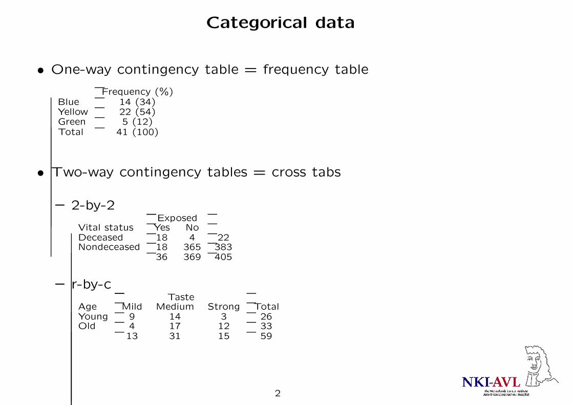
Categorical data

• One-way contingency table = frequency table

Frequency (%)Blue 14 (34)Yellow 22 (54)Green 5 (12)Total 41 (100)

• Two-way contingency tables = cross tabs

– 2-by-2Exposed

Vital status Yes NoDeceased 18 4 22Nondeceased 18 365 383

36 369 405

– r-by-cTaste

Age Mild Medium Strong TotalYoung 9 14 3 26Old 4 17 12 33

13 31 15 59

2

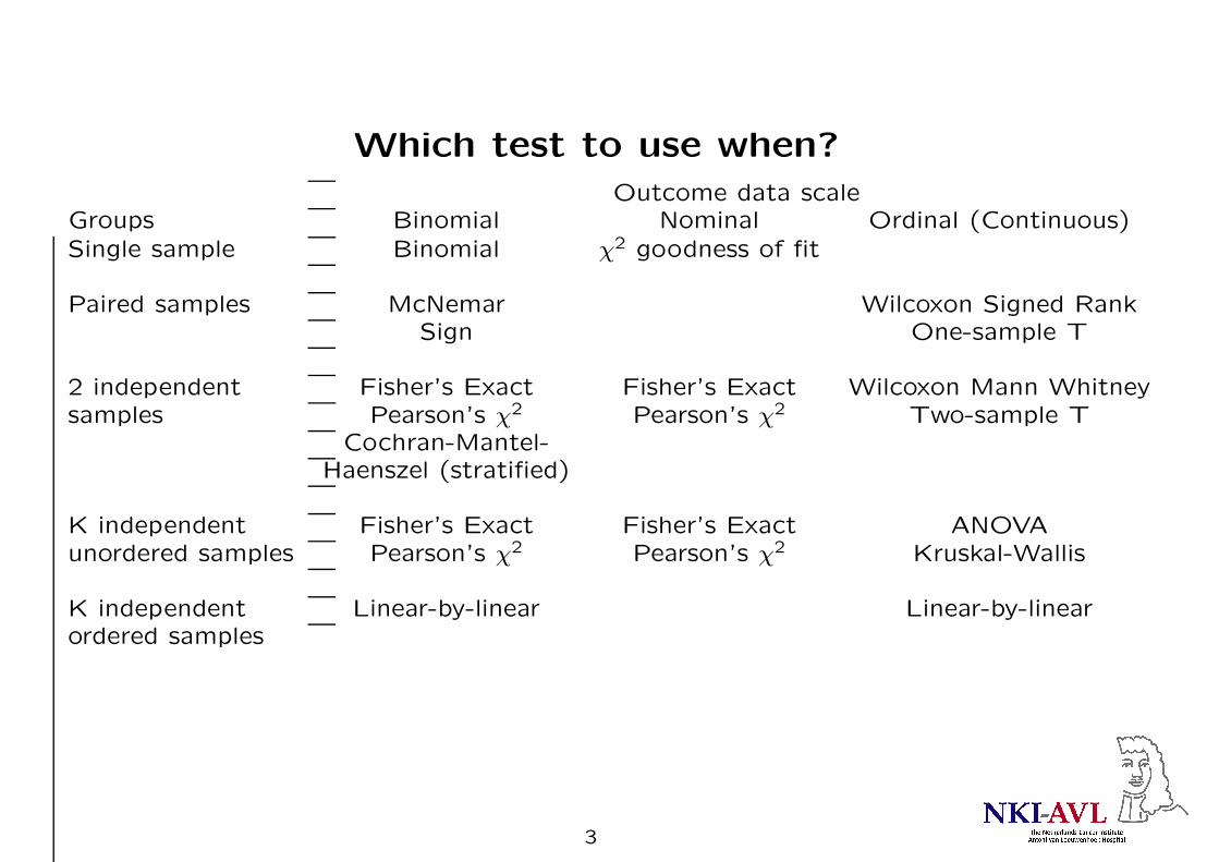
Which test to use when?

Outcome data scaleGroups Binomial Nominal Ordinal (Continuous)Single sample Binomial χ2 goodness of fit

Paired samples McNemar Wilcoxon Signed RankSign One-sample T

2 independent Fisher’s Exact Fisher’s Exact Wilcoxon Mann Whitneysamples Pearson’s χ2 Pearson’s χ2 Two-sample T

Cochran-Mantel-Haenszel (stratified)

K independent Fisher’s Exact Fisher’s Exact ANOVAunordered samples Pearson’s χ2 Pearson’s χ2 Kruskal-Wallis

K independent Linear-by-linear Linear-by-linearordered samples

3

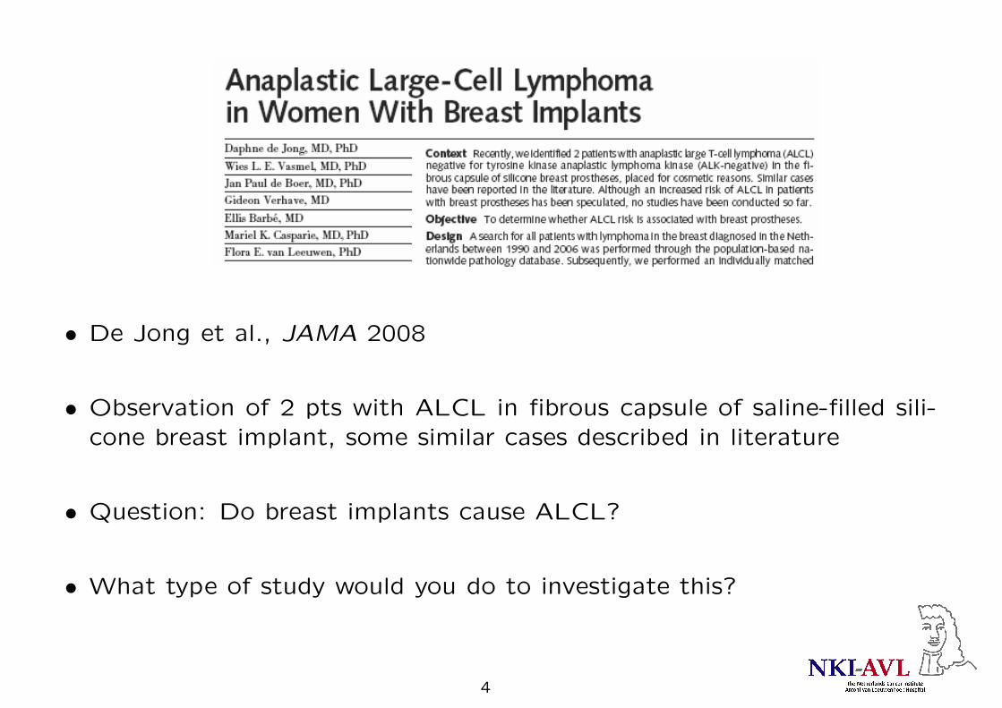
• De Jong et al., JAMA 2008

• Observation of 2 pts with ALCL in fibrous capsule of saline-filled sili-

cone breast implant, some similar cases described in literature

• Question: Do breast implants cause ALCL?

• What type of study would you do to investigate this?

4

Answer: Case-control study

• Identified all 429 pts with biopsy-proven primary NHL of the breast in

1990–2006 in NL from PALGA

• 11/389 female pts had ALCL

• 11 subjects with other lymphomas in the breast as controls

• Medical records obtained for all cases & controls

• Presence of breast implant asked by letter to treating physician

5

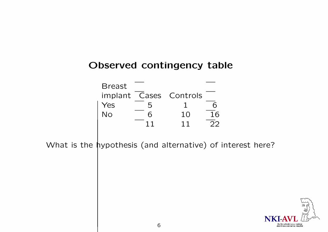
Observed contingency table

Breastimplant Cases Controls

Yes 5 1 6No 6 10 16

11 11 22

What is the hypothesis (and alternative) of interest here?

6

Observed contingency table

Breastimplant Cases ControlsYes 5 1 6No 6 10 16

11 11 22

H0: % pts w/ breast implants equal among cases & controlsH1: proportions not equal

equivalently:

H0: no association between breast implants & case statusH1: association

7

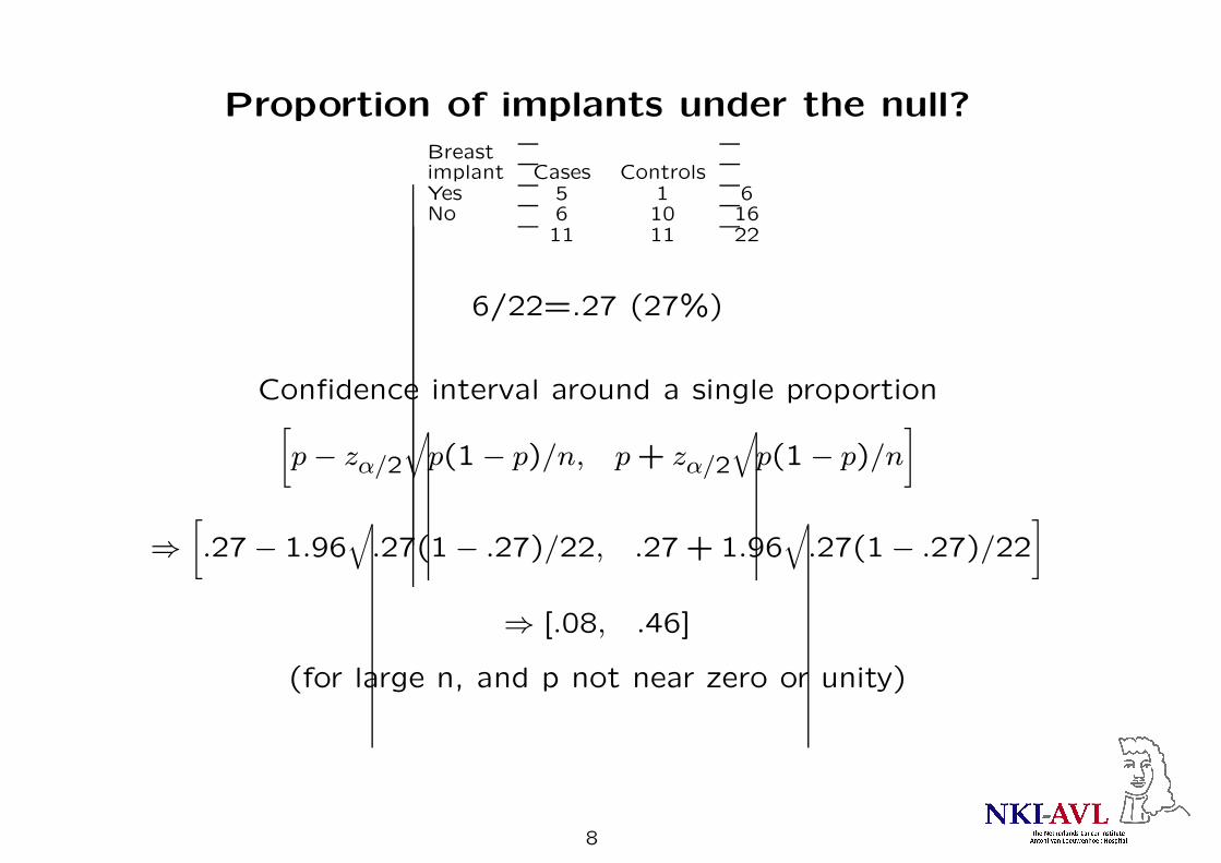
Proportion of implants under the null?

Breastimplant Cases ControlsYes 5 1 6No 6 10 16

11 11 22

6/22=.27 (27%)

Confidence interval around a single proportion[

p− zα/2

√

p(1− p)/n, p+ zα/2

√

p(1− p)/n

]

⇒

[

.27− 1.96√

.27(1− .27)/22, .27+ 1.96√

.27(1− .27)/22

]

⇒ [.08, .46]

(for large n, and p not near zero or unity)

8

CI around single proportion in SPSS1

Dataset alcl_small_casecontrol.sav

9

Back to hypothesis: Pearson chi-square test

Compare observed table w/ expected table under the null

Breast Observed Expectedimplant Cases Controls Cases Controls

Yes 5 1 11*6/22=3 11*6/22=3 6No 6 10 11*16/22=8 11*16/22=8 16

11 11 11 11 22

∑

cells

(|O −E| − 1/2)2

E> χ2

(#rows−1)∗(#columns−1),.95

where O & E are observed & expected frequencies, respectively, for each

cell in 2× 2 contingency table; 1/2 is continuity or Yates’ correction

(little difference unless n < 40 or Es very small)

Here:

(|5−3|− .5)2/3+(|1−3|− .5)2/3+(|6−8|− .5)2/8+(|10−8|− .5)2/8 = 2.06

at (2–1)*(2–1)=1 degrees of freedom

10

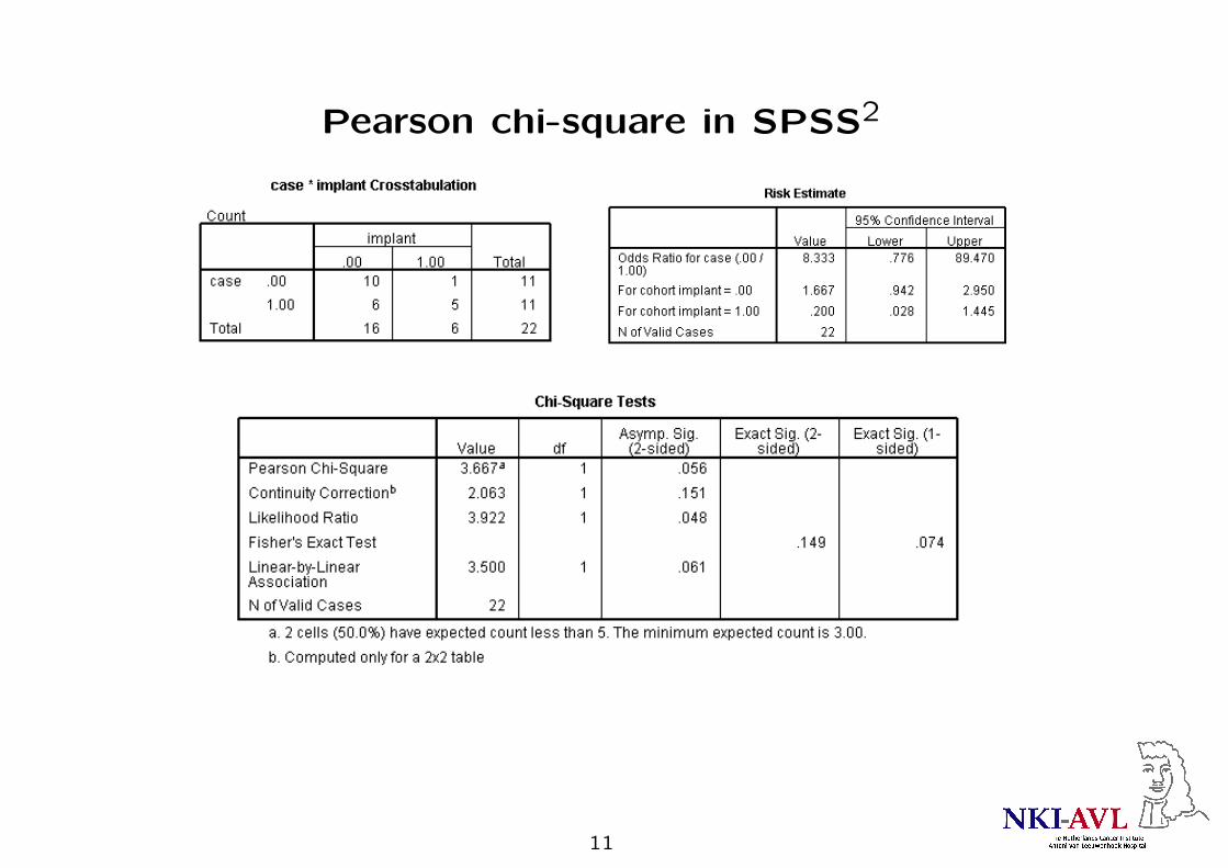
Pearson chi-square in SPSS2

11

Chi-square tests

• Pearson: based on O-E under independence

• Goodness of fit: same as Pearson, but can be used with E based on

specific distribution other than independence

• Can all be extended to r-by-c tables w/ DF=(r–1)*(c–1)

• Chi-square tests are asymptotic tests (for large N)

for small N: Fisher’s exact test

12

An example of Fisher’s exact test

Observed Next Strongesttable stronger table

7 2 9 8 1 9 9 0 95 6 11 4 7 11 3 8 1112 8 20 12 8 20 12 8 20

• Obtain tables stronger than the observed table by reducing the cell

with the lowest count by 1 in steps

• Compute the probability for each table P = (a+b)!(c+d)!(a+c)!(b+d)!N !a!b!c!d!

Pobserved = 9!11!12!8!20!7!2!5!6! = .132

Pstronger = 9!11!12!8!20!8!1!4!7! = .024

Pstrongest = 9!11!12!8!20!9!0!3!8! = .001

Ptotal (one-tailed) = .157

13

Interpretation of Fisher’s exact test

• p = .157, i.e., there is a 15.7% chance under the null that, given the

sample size and the margins, we would get a table as strong or stronger

as the observed table by chance alone

• At α = .05, distribution in observed table is not significantly different

from independence

• Possible for r-by-c tables

• 2-tailed p is sum of probabilities of all tables with p equal or less than

the observed p

14

Is a 2-by-2 analysis sufficient? Confounding?

• A variable correlated with the variable of interest (e.g., exposure or

treatment) and with the outcome is a potential confounder

• E.g., age and calendar year of diagnosis are potential confounders of

the association between breast implants & ALCL

1. Prevalence of breast implants is increasing with calendar year

2. ALCL is more common at older age

3. ALCL cases have fewer breast implants than random sample of non-

ALCL cases: apparent protective effect, but due to confounding bias

15

ALCL study: matching to control confounding

• 11 controls matched to cases by age at DX (within 5 yrs) & yr of DX

(within 2 yrs)

• More specifically: for each case, one woman is randomly chosen from all

women with an age at DX within 5 yrs of that of the case & diagnosed

within 2 yrs of the case

16

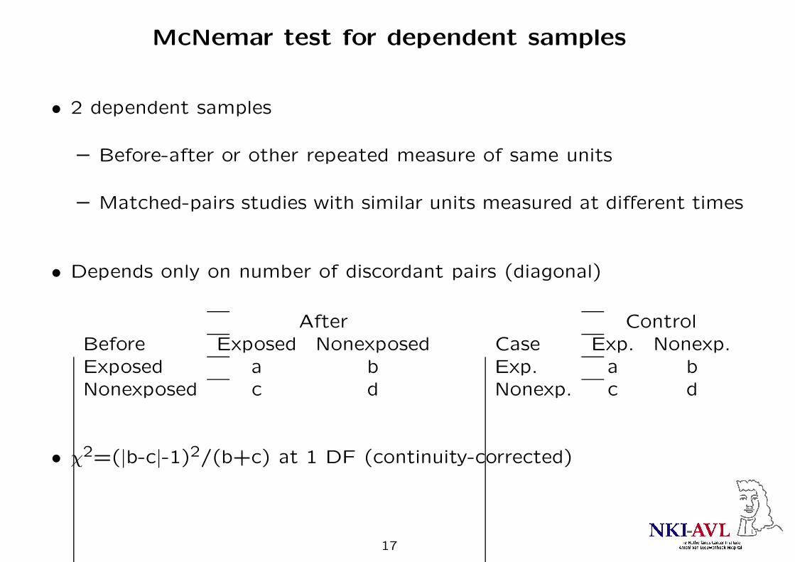
McNemar test for dependent samples

• 2 dependent samples

– Before-after or other repeated measure of same units

– Matched-pairs studies with similar units measured at different times

• Depends only on number of discordant pairs (diagonal)

After ControlBefore Exposed Nonexposed Case Exp. Nonexp.Exposed a b Exp. a bNonexposed c d Nonexp. c d

• χ2=(|b-c|-1)2/(b+c) at 1 DF (continuity-corrected)

17

• Discordant pairs split evenly → evidence that overall proportion about

the same for both raters

• Discordant pairs skewed in one direction (e.g., more yes/no than no/yes)

→ evidence that overall proportion of yeses higher for one rater than

the other

• Multivariate analogon to McNemar is conditional logistic regression

18

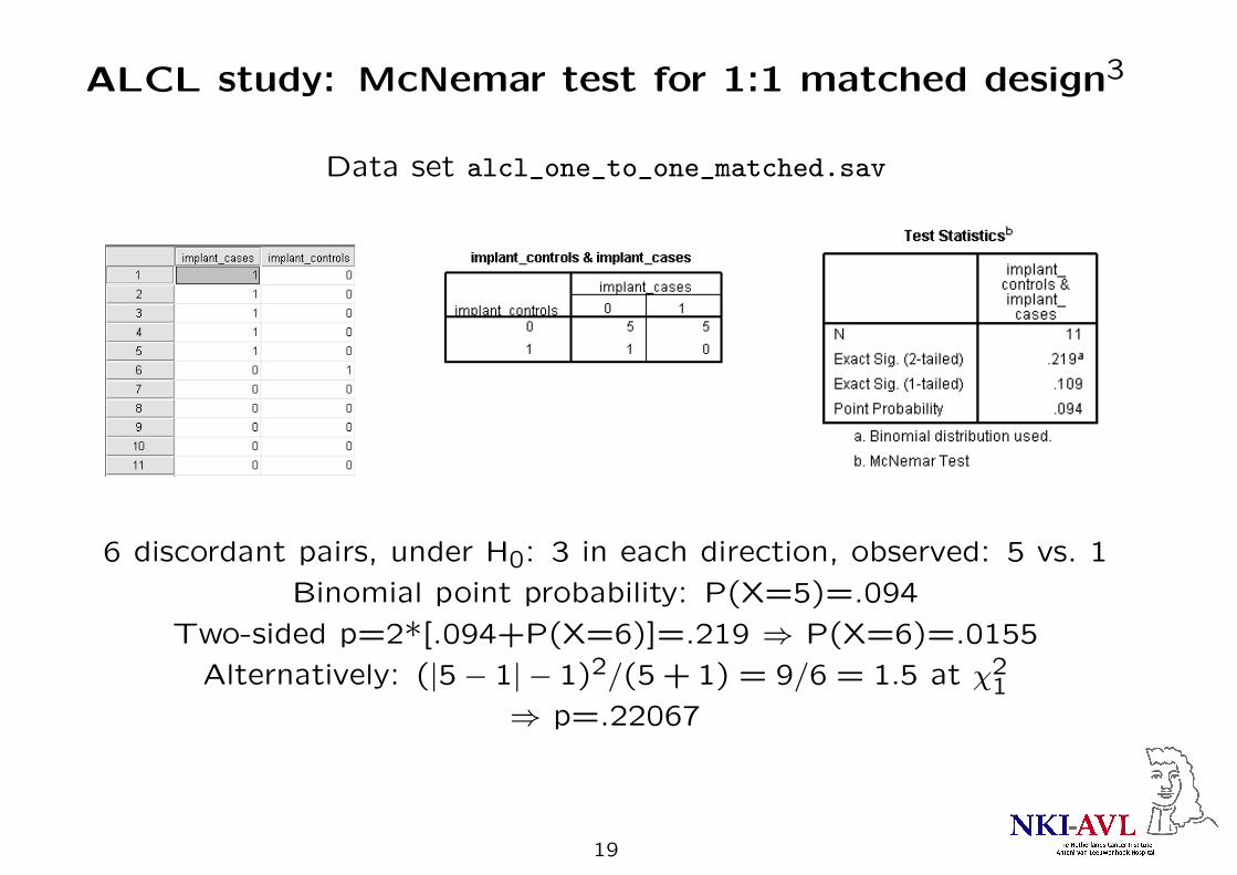
ALCL study: McNemar test for 1:1 matched design3

Data set alcl_one_to_one_matched.sav

6 discordant pairs, under H0: 3 in each direction, observed: 5 vs. 1

Binomial point probability: P(X=5)=.094

Two-sided p=2*[.094+P(X=6)]=.219 ⇒ P(X=6)=.0155

Alternatively: (|5− 1| − 1)2/(5 + 1) = 9/6 = 1.5 at χ21

⇒ p=.22067

19

Exact vs. asymptotic procedures

• Most standard statistical tests assume test statistic is asymptotically

normally distributed (large N)

• May not be true for small studies

• Exact tests based on permutation or Monte Carlo simulation (resam-

pling)

• Exact p-values smaller or larger than asymptotic p-values

• Included in most statistical software packages

20

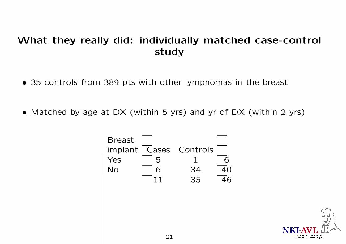
What they really did: individually matched case-controlstudy

• 35 controls from 389 pts with other lymphomas in the breast

• Matched by age at DX (within 5 yrs) and yr of DX (within 2 yrs)

Breastimplant Cases Controls

Yes 5 1 6No 6 34 40

11 35 46

21

• McNemar only for matched pairs (1:1)

• Standard 2-by-2 analysis4

Crude OR=28.3, asymptotic 95% CI 2.8–287.1, p=.002

• Conditional logistic regression (asymptotic) for >1 controls per case

via Cox regression5

OR=18.2, 95% CI 2.1–156.8, p=.008 (reported)

• Matching is controlling for confounding at the design stage

• Confounding can also be controlled, however less efficiently, at the anal-

ysis stage: Cochran-Mantel-Haenszel test or adjustment in regression

models

22

Updated results 2018

23

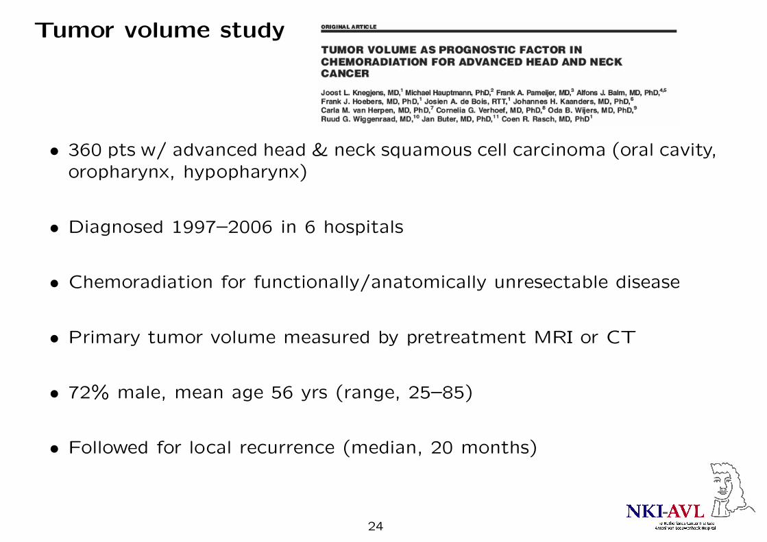
Tumor volume study

• 360 pts w/ advanced head & neck squamous cell carcinoma (oral cavity,

oropharynx, hypopharynx)

• Diagnosed 1997–2006 in 6 hospitals

• Chemoradiation for functionally/anatomically unresectable disease

• Primary tumor volume measured by pretreatment MRI or CT

• 72% male, mean age 56 yrs (range, 25–85)

• Followed for local recurrence (median, 20 months)

24

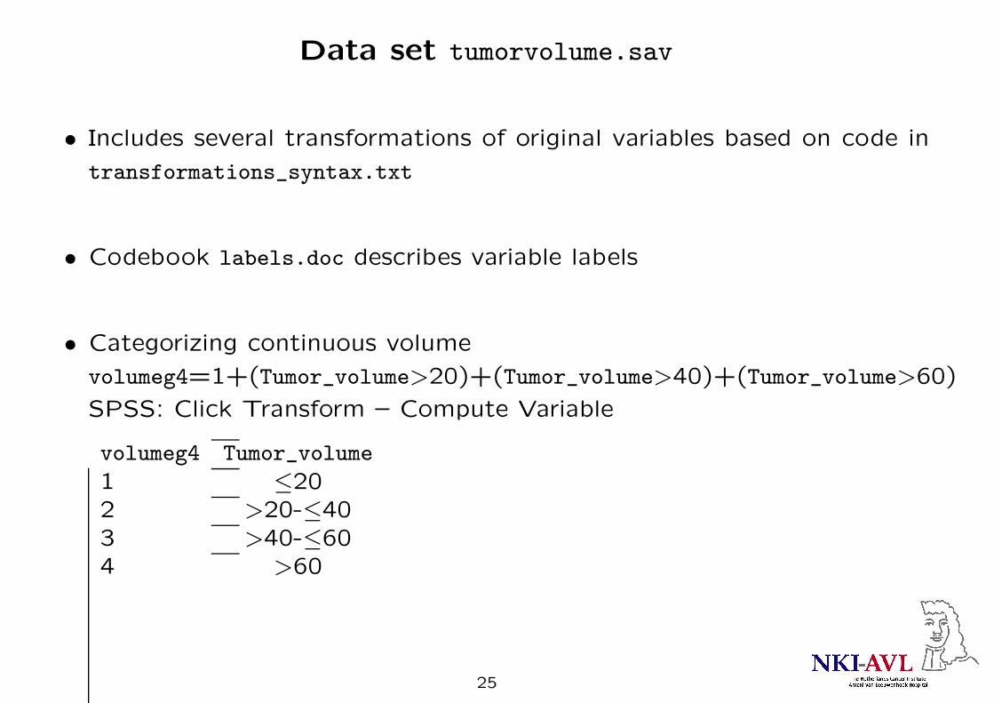
Data set tumorvolume.sav

• Includes several transformations of original variables based on code in

transformations_syntax.txt

• Codebook labels.doc describes variable labels

• Categorizing continuous volume

volumeg4=1+(Tumor_volume>20)+(Tumor_volume>40)+(Tumor_volume>60)

SPSS: Click Transform – Compute Variable

volumeg4 Tumor_volume

1 ≤202 >20-≤403 >40-≤604 >60

25

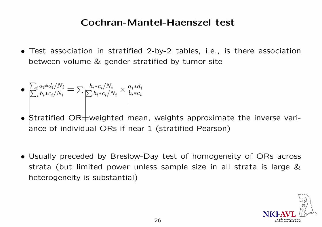
Cochran-Mantel-Haenszel test

• Test association in stratified 2-by-2 tables, i.e., is there association

between volume & gender stratified by tumor site

•∑

i ai∗di/Ni∑

i bi∗ci/Ni=

∑ bi∗ci/Ni∑

bi∗ci/Ni× ai∗di

bi∗ci

• Stratified OR=weighted mean, weights approximate the inverse vari-

ance of individual ORs if near 1 (stratified Pearson)

• Usually preceded by Breslow-Day test of homogeneity of ORs across

strata (but limited power unless sample size in all strata is large &

heterogeneity is substantial)

26

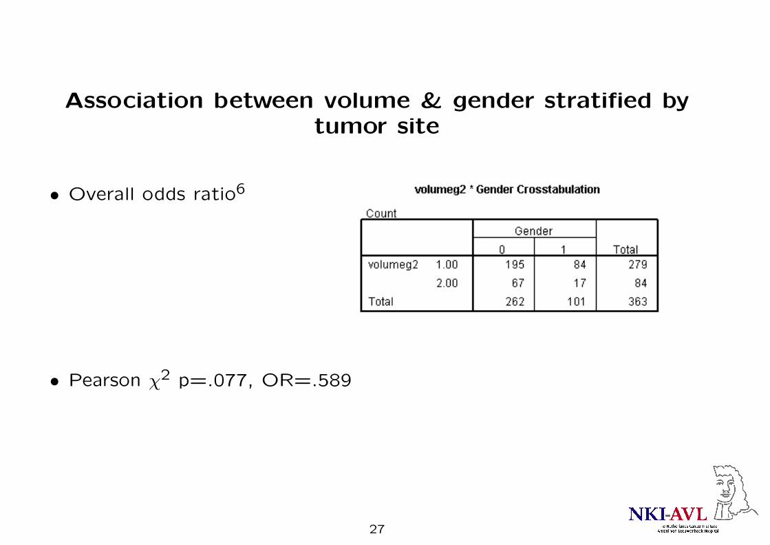
Association between volume & gender stratified bytumor site

• Overall odds ratio6

• Pearson χ2 p=.077, OR=.589

27

• Test of homogeneity, common OR & CMH test7

• Common OR=.588 ⇒ no confounding by tumor site

28

Chi-square goodness of fit test with specifieddistribution

• Question: Is infusion side (single- vs. double-sided) distributed 50-50?

• Provide SPSS with expected proportions: 50-508

• p=.292: data are consistent with 50-50 split

29

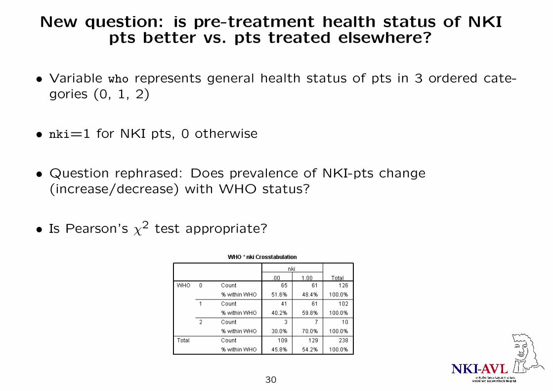
New question: is pre-treatment health status of NKIpts better vs. pts treated elsewhere?

• Variable who represents general health status of pts in 3 ordered cate-gories (0, 1, 2)

• nki=1 for NKI pts, 0 otherwise

• Question rephrased: Does prevalence of NKI-pts change(increase/decrease) with WHO status?

• Is Pearson’s χ2 test appropriate?

30

Linear-by-linear association test9

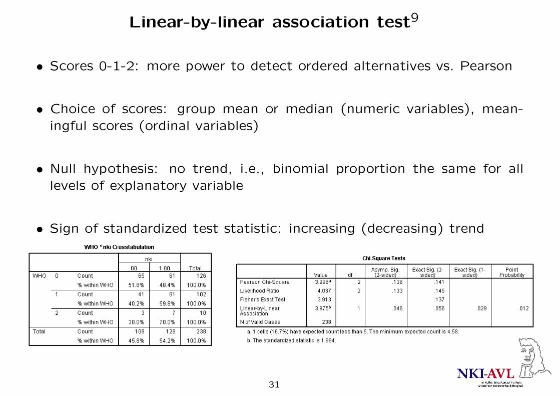
• Scores 0-1-2: more power to detect ordered alternatives vs. Pearson

• Choice of scores: group mean or median (numeric variables), mean-

ingful scores (ordinal variables)

• Null hypothesis: no trend, i.e., binomial proportion the same for all

levels of explanatory variable

• Sign of standardized test statistic: increasing (decreasing) trend

31

Association between tumor-volume & N-stage?

• N-stage as row scores & tumor volume categories as column scores10

• Trend test more powerful than Pearson χ2: p=.008 vs. .063

32

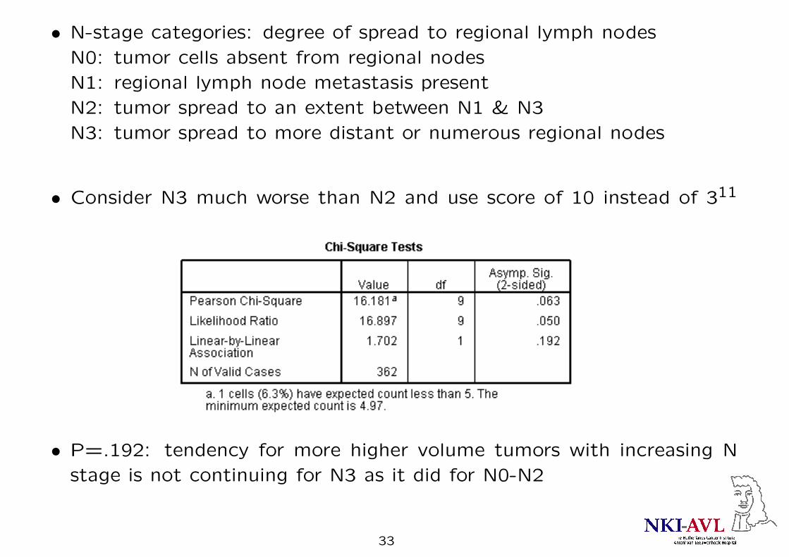
• N-stage categories: degree of spread to regional lymph nodes

N0: tumor cells absent from regional nodes

N1: regional lymph node metastasis present

N2: tumor spread to an extent between N1 & N3

N3: tumor spread to more distant or numerous regional nodes

• Consider N3 much worse than N2 and use score of 10 instead of 311

• P=.192: tendency for more higher volume tumors with increasing N

stage is not continuing for N3 as it did for N0-N2

33

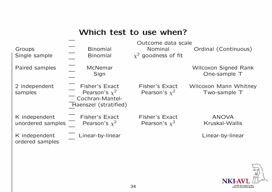
Which test to use when?

Outcome data scaleGroups Binomial Nominal Ordinal (Continuous)Single sample Binomial χ2 goodness of fit

Paired samples McNemar Wilcoxon Signed RankSign One-sample T

2 independent Fisher’s Exact Fisher’s Exact Wilcoxon Mann Whitneysamples Pearson’s χ2 Pearson’s χ2 Two-sample T

Cochran-Mantel-Haenszel (stratified)

K independent Fisher’s Exact Fisher’s Exact ANOVAunordered samples Pearson’s χ2 Pearson’s χ2 Kruskal-Wallis

K independent Linear-by-linear Linear-by-linearordered samples

34

SPSS code (syntax and clicking)

1. CI around single proportion

Click Analyze – Descriptive Statistics – Frequencies and select variable

implant. Click Transform – Compute Variable and fill in an arbitrary

new variable name with value 1. Click Analyze – Descriptive Statistics –

Ratio and select variable implant and the new variable. Click Statistics

and request confidence intervals.

FREQUENCIES VARIABLES=implant/ORDER=ANALYSIS.

COMPUTE one=1.

EXECUTE.

RATIO STATISTICS implant WITH one

/MISSING=EXCLUDE

/PRINT=CIN(95) MEAN.

35

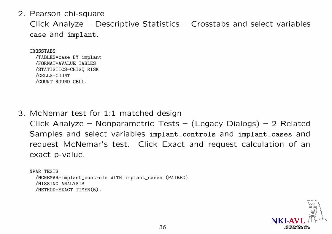
2. Pearson chi-square

Click Analyze – Descriptive Statistics – Crosstabs and select variables

case and implant.

CROSSTABS/TABLES=case BY implant/FORMAT=AVALUE TABLES/STATISTICS=CHISQ RISK/CELLS=COUNT/COUNT ROUND CELL.

3. McNemar test for 1:1 matched design

Click Analyze – Nonparametric Tests – (Legacy Dialogs) – 2 Related

Samples and select variables implant_controls and implant_cases and

request McNemar’s test. Click Exact and request calculation of an

exact p-value.

NPAR TESTS/MCNEMAR=implant_controls WITH implant_cases (PAIRED)/MISSING ANALYSIS/METHOD=EXACT TIMER(5).

36

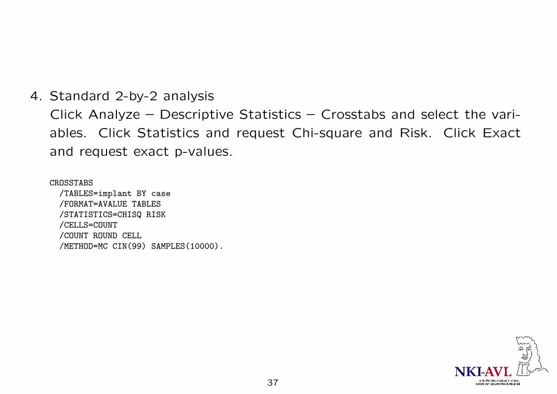
4. Standard 2-by-2 analysis

Click Analyze – Descriptive Statistics – Crosstabs and select the vari-

ables. Click Statistics and request Chi-square and Risk. Click Exact

and request exact p-values.

CROSSTABS

/TABLES=implant BY case

/FORMAT=AVALUE TABLES

/STATISTICS=CHISQ RISK/CELLS=COUNT

/COUNT ROUND CELL

/METHOD=MC CIN(99) SAMPLES(10000).

37

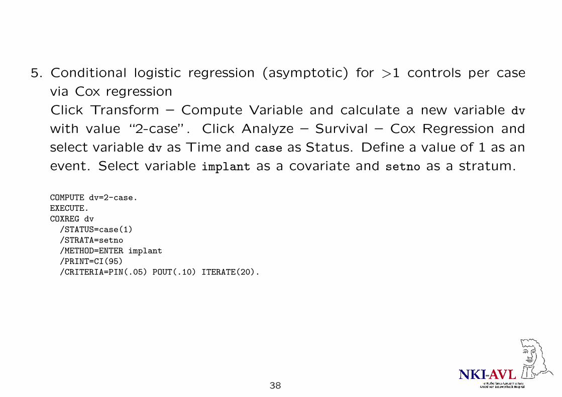
5. Conditional logistic regression (asymptotic) for >1 controls per case

via Cox regression

Click Transform – Compute Variable and calculate a new variable dv

with value “2-case”. Click Analyze – Survival – Cox Regression and

select variable dv as Time and case as Status. Define a value of 1 as an

event. Select variable implant as a covariate and setno as a stratum.

COMPUTE dv=2-case.

EXECUTE.

COXREG dv

/STATUS=case(1)

/STRATA=setno/METHOD=ENTER implant

/PRINT=CI(95)

/CRITERIA=PIN(.05) POUT(.10) ITERATE(20).

38

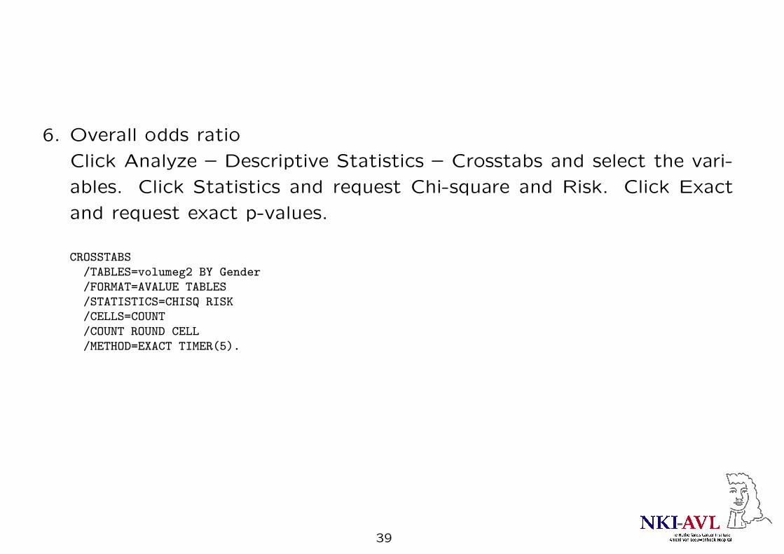
6. Overall odds ratio

Click Analyze – Descriptive Statistics – Crosstabs and select the vari-

ables. Click Statistics and request Chi-square and Risk. Click Exact

and request exact p-values.

CROSSTABS

/TABLES=volumeg2 BY Gender

/FORMAT=AVALUE TABLES

/STATISTICS=CHISQ RISK/CELLS=COUNT

/COUNT ROUND CELL

/METHOD=EXACT TIMER(5).

39

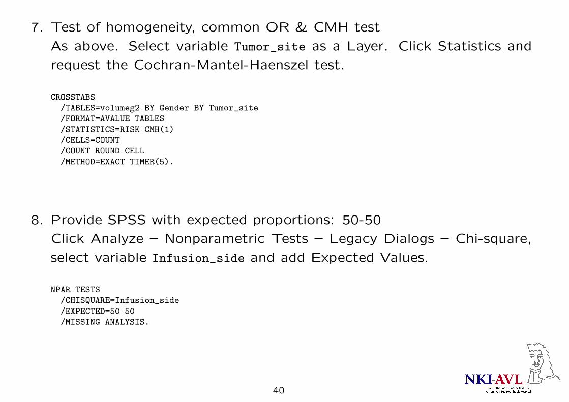
7. Test of homogeneity, common OR & CMH test

As above. Select variable Tumor_site as a Layer. Click Statistics and

request the Cochran-Mantel-Haenszel test.

CROSSTABS

/TABLES=volumeg2 BY Gender BY Tumor_site

/FORMAT=AVALUE TABLES/STATISTICS=RISK CMH(1)

/CELLS=COUNT

/COUNT ROUND CELL

/METHOD=EXACT TIMER(5).

8. Provide SPSS with expected proportions: 50-50

Click Analyze – Nonparametric Tests – Legacy Dialogs – Chi-square,

select variable Infusion_side and add Expected Values.

NPAR TESTS

/CHISQUARE=Infusion_side

/EXPECTED=50 50

/MISSING ANALYSIS.

40

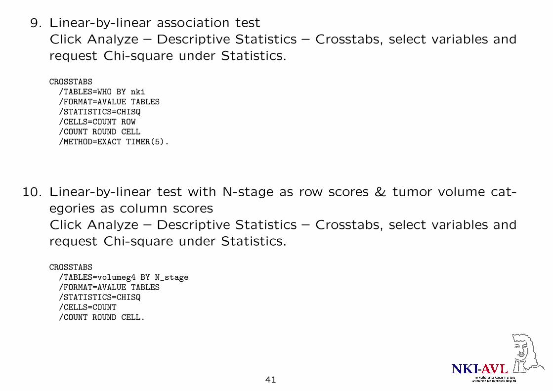
9. Linear-by-linear association test

Click Analyze – Descriptive Statistics – Crosstabs, select variables and

request Chi-square under Statistics.

CROSSTABS/TABLES=WHO BY nki/FORMAT=AVALUE TABLES/STATISTICS=CHISQ/CELLS=COUNT ROW/COUNT ROUND CELL/METHOD=EXACT TIMER(5).

10. Linear-by-linear test with N-stage as row scores & tumor volume cat-

egories as column scores

Click Analyze – Descriptive Statistics – Crosstabs, select variables and

request Chi-square under Statistics.

CROSSTABS/TABLES=volumeg4 BY N_stage/FORMAT=AVALUE TABLES/STATISTICS=CHISQ/CELLS=COUNT/COUNT ROUND CELL.

41

11. Linear-by-linear test with score of 10 instead of 3 for N3

Click Transform – Compute Variable and create variable n_stage_new

as n_stage*(n_stage<3)+10*(n_stage=3). Click Analyze – Descriptive

Statistics – Crosstabs, select variables volumeg4 and n_stage_new and

request Chi-square under Statistics.

COMPUTE n_stage_new=n_stage*(n_stage<3)+10*(n_stage=3).

EXECUTE.

CROSSTABS/TABLES=volumeg4 BY n_stage_new

/FORMAT=AVALUE TABLES

/STATISTICS=CHISQ

/CELLS=COUNT

/COUNT ROUND CELL.

42