Two Population Means Hypothesis Testing and Confidence Intervals With Known Standard Deviations.
21
Two Population Means Two Population Means Hypothesis Testing and Hypothesis Testing and Confidence Intervals Confidence Intervals With Known Standard With Known Standard Deviations Deviations
-
date post
20-Dec-2015 -
Category
Documents
-
view
219 -
download
0
Transcript of Two Population Means Hypothesis Testing and Confidence Intervals With Known Standard Deviations.

Two Population MeansTwo Population Means
Hypothesis Testing and Hypothesis Testing and Confidence IntervalsConfidence Intervals
With Known Standard DeviationsWith Known Standard Deviations

SITUATION: 2 PopulationsSITUATION: 2 Populations
Population 1
Mean = 1
St’d Dev. = 1
Population 2
Mean = 2
St’d Dev. = 2
Salaries in Chicago Salaries in St. Louis
Women’s Test Scores Men’s Test Scores
Lakers Attendance Clippers Attendance
Anaheim Sales Irvine Sales

KEY ASSUMPTIONSKEY ASSUMPTIONSSampling is done from two populations.
– Population 1 has mean µ1 and variance σ12.
– Population 2 has mean µ2 and variance σ22.
– A sample of size n1 will be taken from population 1.
– A sample of size n2 will be taken from population 2.
– Sampling is random and both samples are drawn independently.
– Either the sample sizes will be large or the populations are assumed to be normally distribution.
1
21
1
111 n
σ variance,
n
σ deviation standard ,μ mean :X variableRandom
2
22
2
222 n
σ variance,
n
σ deviation standard ,μ mean :X variableRandom

The ProblemThe Problem1 and 2 are unknown
1 and 2 may or may not be known
(In this module we assume they are known.)
OBJECTIVESOBJECTIVES• Test whether 1 > 2 (by a certain amount)
– or whether 1 2
• Determine a confidence interval for the difference in the means: 1 - 2

21 XX
Key Concepts About the Key Concepts About the Random Variable .Random Variable .
• is the difference in two sample means.1. Its meanmean is the difference of the two individual means:
2. If the variables are independent (which we assumed), the variancevariance (not the standard deviation) of the random variable of the differences = the sum (not the difference) of the two variances:
3. Thus its standard deviationstandard deviation is:
4. Its distributiondistribution is:• Normal if σ1 and σ2 are known • t if σ1 and σ2 are unknown
21 XX
2
22
1
21
n
σ
n
σ
21 μμ
2
22
1
21
n
σ
n
σ

Random Variable XDistribution normal normal normal
Mean 1 2
Standard Deviation
21 XX X
n
σ
2
22
1
21
n
σ
n
σ
21 XX ,X X, Variable Random

Hypothesis Test Statistics forHypothesis Test Statistics forDifference in Means, Known Difference in Means, Known σσ’s’s
• We will be performing hypothesis tests with null hypotheses, H0, of the form:
• From the general form of a test statistic, the required test statistic will be:
2
22
1
21
21
nσ
nσ
v)xx(
ErrorStandard
Value) zed(Hypothesi - imate)(Point Estz
HH00: : µµ11 - µ - µ22 = v = v

Confidence Intervals for Confidence Intervals for µµ11 - µ - µ22
Known Known σσ’s’s• Recall the general form of a confidence interval is:
Thus when the σ’s are known this becomes:
(Point Estimate) ± zα/2(Appropriate Standard Error)
2
22
1
21
α/221 n
σ
n
σzxx

EXAMPLEEXAMPLEHypothesis Test: Hypothesis Test: 11, , 2 2 KnownKnown
Test whether starting salaries for secretaries in Chicago are at least $5 more per week than those in St. Louis.
GIVEN:Salaries assumed to be normal
Standard Deviations known: Chicago $10; St. Louis $15
Sample ResultsSampled 100 secretaries in Chicago; 75 secretaries in St. Louis
Sample averages: Chicago - $550, St. Louis -$540

Hypothesis TestHypothesis Test
H0: 1 - 2 = 5
HA: 1 - 2 > 5
Use = .05
Reject H0 (Accept HA) if z > z.05 = 1.645

Calculating zCalculating zRemember
Deviation Standard eAppropriat
Value) zed(HypothesiEstimate)(Point z
2
22
1
21
21
nσ
nσ
5)x-x(z
2.5
75
15
100
10
5540)-(550z
22

ConclusionConclusion
• Since 2.5 > 1.645– It can be concluded that the average starting salary for
secretaries in Chicago is at least $5 per week greater than the average starting salary in St. Louis.
• The p-value:– The area above z= 2.5 on the normal curve = 1 - .9938
= .0062– Since .0062 is low (compared to α), it can be concluded
that the average starting salary for secretaries in Chicago is at least $5 per week greater than the average starting salary in St. Louis.

EXAMPLEEXAMPLEConfidence Interval: Confidence Interval: 11, , 2 2 KnownKnown
• Construct a 95% confidence for the difference in average between weekly starting salaries for secretaries in Chicago and St. Louis.
2
22
1
21
.02521 n
σ
n
σz )x-x(
75
15
100
101.96 540)-(550
22
$10 ± $3.92
$6.08 ↔ $13.92

Excel ApproachExcel Approach
• Suppose, as shown on the next slide the data for Chicago is given in column A (A2:A101) and the data for St. Louis is given in column B (B2:B76).
• The analysis can be done using an entry from the Data Analysis Menu:
z-test: Two Sample for Meansz-test: Two Sample for Means

Select
z-Test: Two Sample For Means
Go to Data
Then Data Analysis
Select
z-Test: Two Sample For Means

For 1-tail tests, input columns so that the test is
a “>” test.Enter
Hypothesized Difference
Enter Variances
Not
Standard Deviations
Check
Labels
Enter
Beginning Cell
For Output
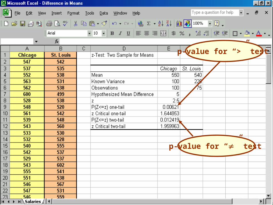
p-value for “>” test
p-value for “” test

=(E4-F4)-NORMSINV(0.975)*SQRT(E5/E6+F5/F6)
Highlight formula in cell E15—press F4.
Drag to cell E16 and change “-” to “+”.

Estimating Sample SizesEstimating Sample Sizes• Usual Assumptions:
– Same sample size from each pop.: n1 = n2 = n
– Standard deviations, 1 2 known
• Calculate n from the “±” part of the confidence interval for known 1and 2
En
σσ1.96
n
σ
n
σ1.96
22
21
22
21

ExampleExample• How many workers would have to be
surveyed in Chicago and St. Louis to estimate the true average difference in starting weekly salary to within $3?
surveyd! be would total workers278
cityeach in 139138.72(11.78)n
78.113
3251.96 n
3n
15101.96
n
σ
n
σ1.96
2
2222
21

ReviewReview• Mean and standard deviation for X1 -X2
• Assumptions for tests and confidence intervals
• z-tests for differences in means when 1 and 2 are known: – By Formula– By Excel data analysis tool
• Confidence intervals for differences in means when 1 and 2 are known:
– By Formula– By Excel data analysis tool
• Estimating Sample Sizes