Confidence Intervals - University Corporation for ...ericg/GillelandCItalkVxColloquium2010.pdf ·...

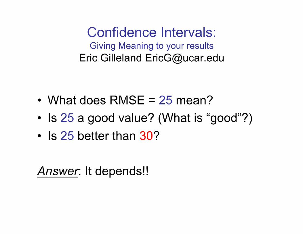
Confidence Intervals: Giving Meaning to your results

Eric Gilleland [email protected]

•  What does RMSE = 25 mean? •  Is 25 a good value? (What is “good”?) •  Is 25 better than 30?

Answer: It depends!!

copyright 2009, UCAR, all rights reserved.

)


Accounting for Uncertainty •  Observational •  Model

–  Model parameters –  Physics

•  Sampling –  Verification statistic is a realization of a random

process –  What if the experiment were re-run under identical

conditions?


Hypothesis Testing and Confidence Intervals

•  Hypothesis testing –  Given a null hypothesis (e.g., “Model forecast is un-biased”),

is there enough evidence to reject it? –  Can be One- or two-sided –  Test is against a single null hypothesis.

•  Confidence intervals –  Related to hypothesis tests, but more useful. –  How confident are we that the true value of the statistic (e.g.,

bias) is different from a particular value?


Example: The difference in bias between two models is 0.01.

Hypothesis test: Is this different from zero?

Confidence interval: Does zero fall within the interval? Does 0.5 fall within the interval?

Hypothesis Testing and Confidence Intervals


Confidence Intervals (CI’s) “If we re-run the experiment 100

times, and create 100 (1-α)100% CI’s, then we expect the true value of the parameter to fall inside (1-α)100 of the intervals.”

Example: 95% CI has α=0.05, and it is expected that 95 of the 100 intervals would contain the true parameter.


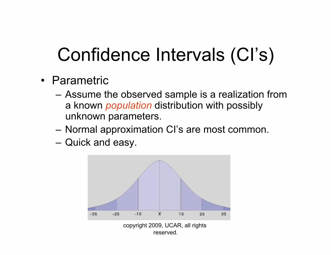
Confidence Intervals (CI’s) •  Parametric

–  Assume the observed sample is a realization from a known population distribution with possibly unknown parameters.

–  Normal approximation CI’s are most common. –  Quick and easy.


Confidence Intervals (CI’s) •  Nonparametric

–  Assume the distribution of the observed sample is representative of the population distribution.

–  Bootstrap CI’s are most common. –  Can be computationally intensive, but easy

enough.

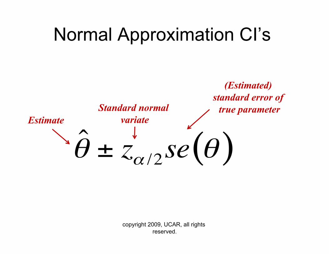
Normal Approximation CI’s


Estimate Standard normal

variate

(Estimated) standard error of

true parameter


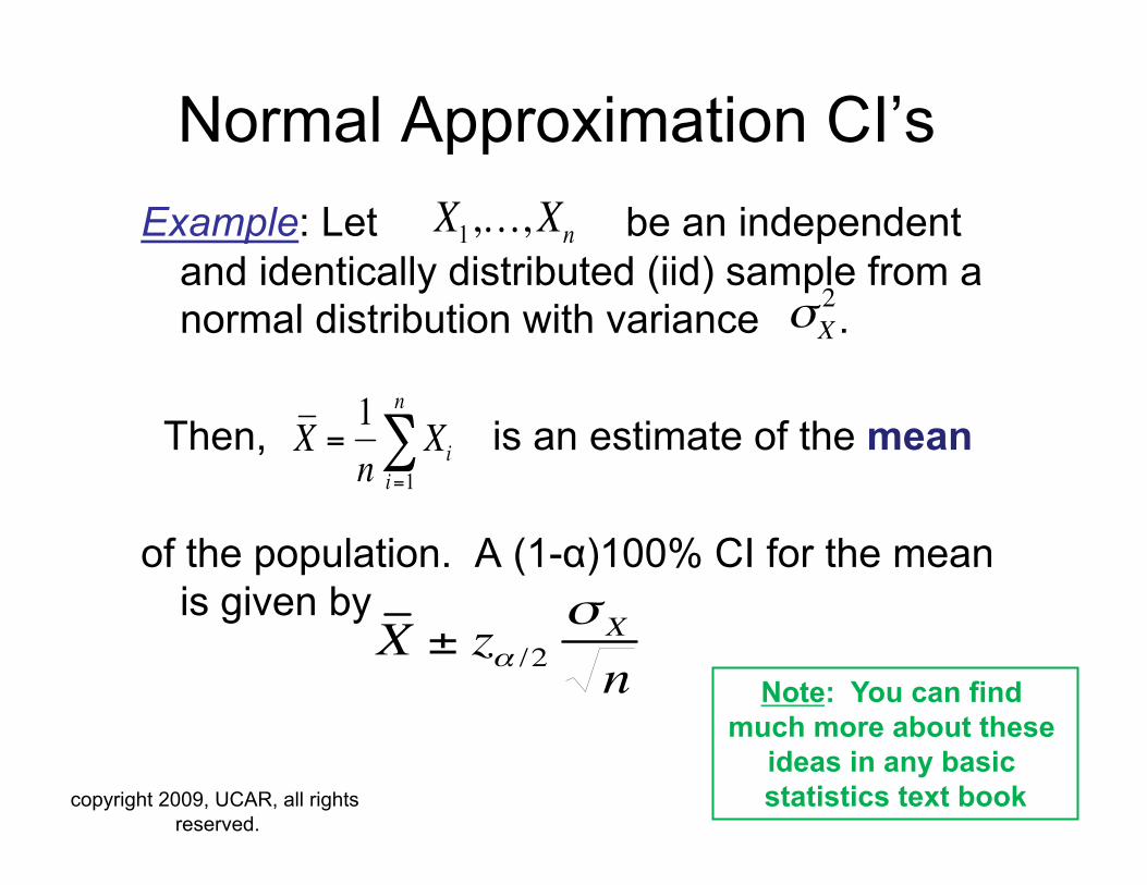
Example: Let be an independent and identically distributed (iid) sample from a normal distribution with variance .

Then, is an estimate of the mean

of the population. A (1-α)100% CI for the mean is given by

Normal Approximation CI’s

Note: You can find much more about these

ideas in any basic statistics text book

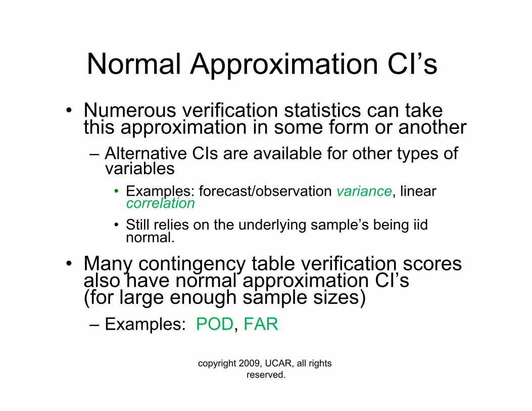
Normal Approximation CI’s •  Numerous verification statistics can take

this approximation in some form or another – Alternative CIs are available for other types of

variables •  Examples: forecast/observation variance, linear

correlation •  Still relies on the underlying sample’s being iid

normal.

•  Many contingency table verification scores also have normal approximation CI’s (for large enough sample sizes) – Examples: POD, FAR


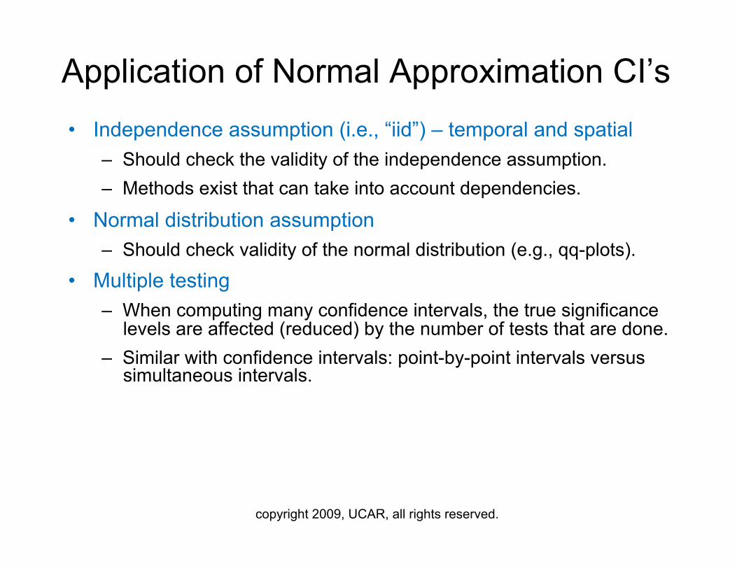
Application of Normal Approximation CI’s •  Independence assumption (i.e., “iid”) – temporal and spatial

–  Should check the validity of the independence assumption. –  Methods exist that can take into account dependencies.

•  Normal distribution assumption –  Should check validity of the normal distribution (e.g., qq-plots).

•  Multiple testing –  When computing many confidence intervals, the true significance

levels are affected (reduced) by the number of tests that are done. –  Similar with confidence intervals: point-by-point intervals versus

simultaneous intervals.


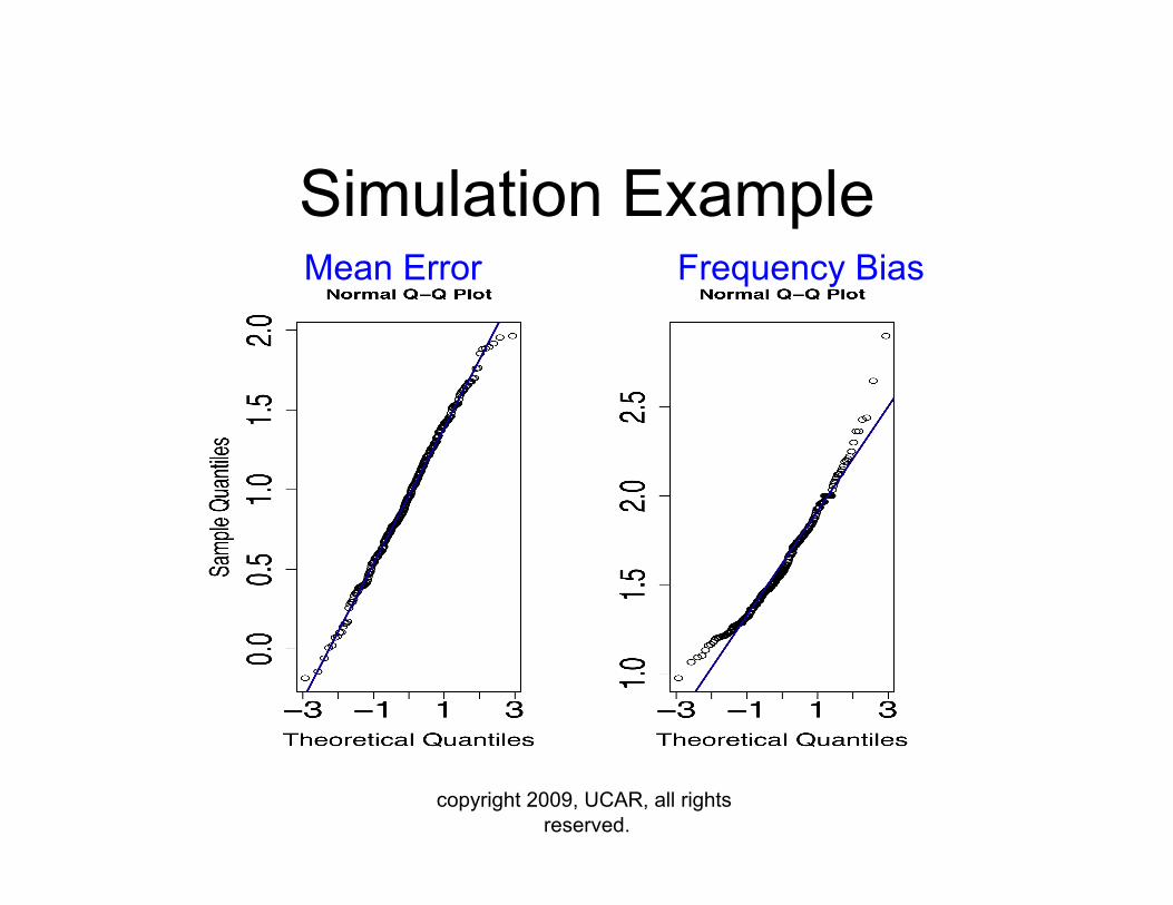
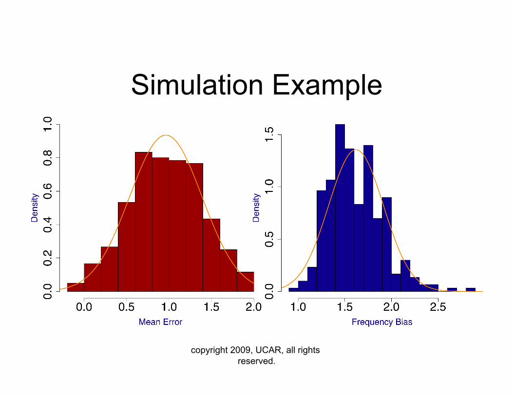
Simulation Example


Mean Error Frequency Bias


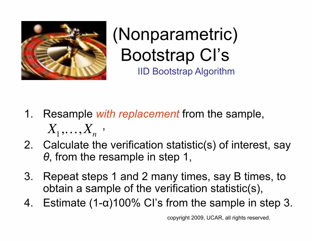
IID Bootstrap Algorithm

(Nonparametric) Bootstrap CI’s

1.  Resample with replacement from the sample, ,

2.  Calculate the verification statistic(s) of interest, say θ, from the resample in step 1,

3.  Repeat steps 1 and 2 many times, say B times, to obtain a sample of the verification statistic(s),

4.  Estimate (1-α)100% CI’s from the sample in step 3.

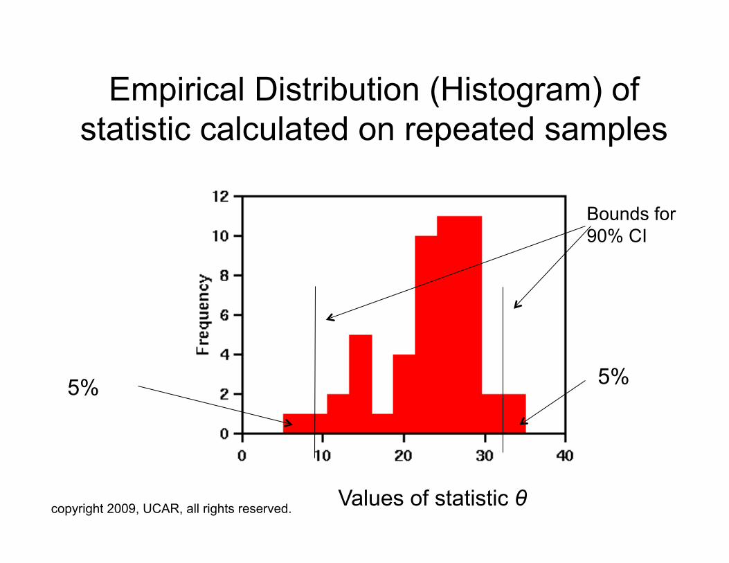
Empirical Distribution (Histogram) of statistic calculated on repeated samples


5% 5%

Bounds for 90% CI

Values of statistic θ


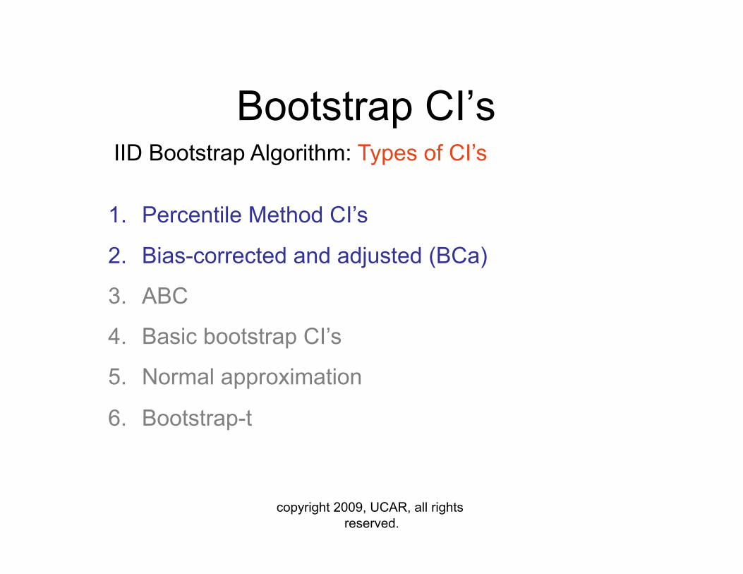
Bootstrap CI’s IID Bootstrap Algorithm: Types of CI’s

1.  Percentile Method CI’s

2.  Bias-corrected and adjusted (BCa)

3.  ABC

4.  Basic bootstrap CI’s

5.  Normal approximation

6.  Bootstrap-t


Simulation Example


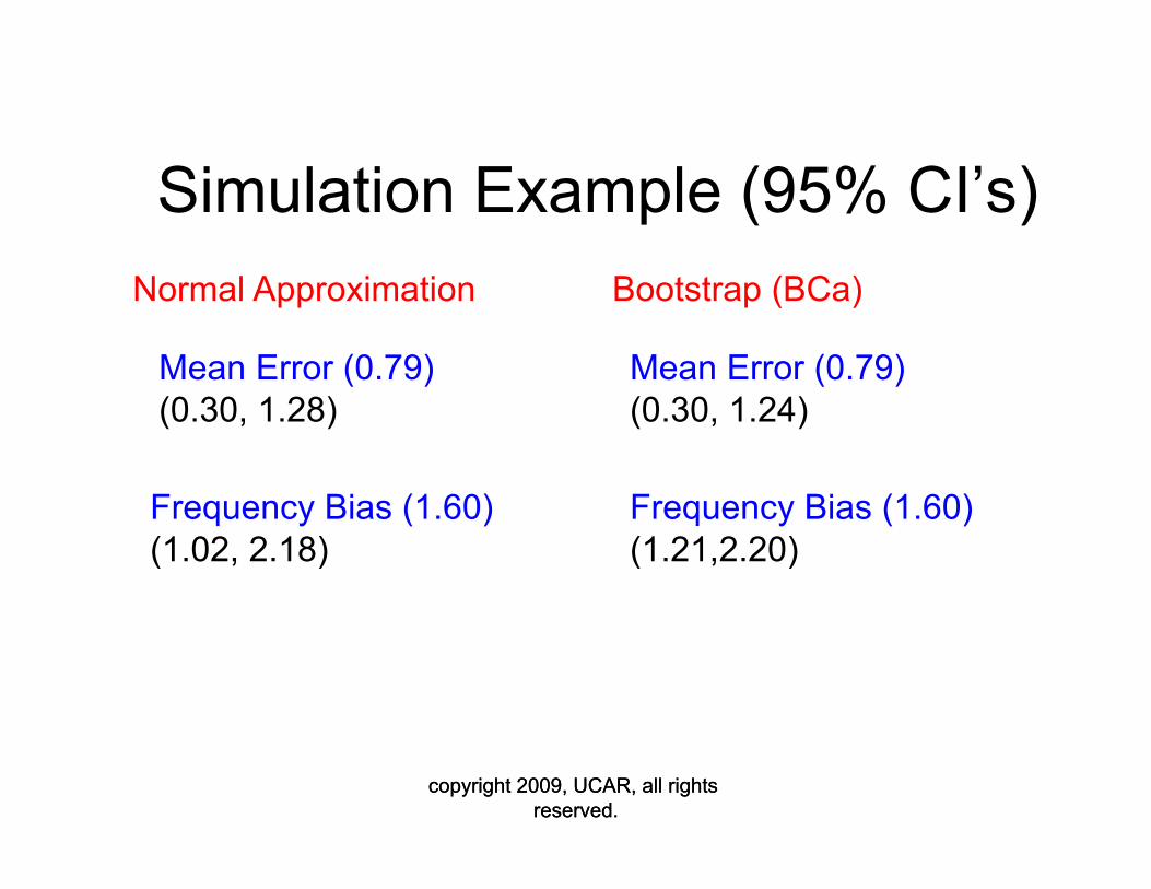
Simulation Example (95% CI’s)


Mean Error (0.79) (0.30, 1.28)

Normal Approximation

Frequency Bias (1.60) (1.02, 2.18)

Bootstrap (BCa)

Mean Error (0.79) (0.30, 1.24)

Frequency Bias (1.60) (1.21,2.20)

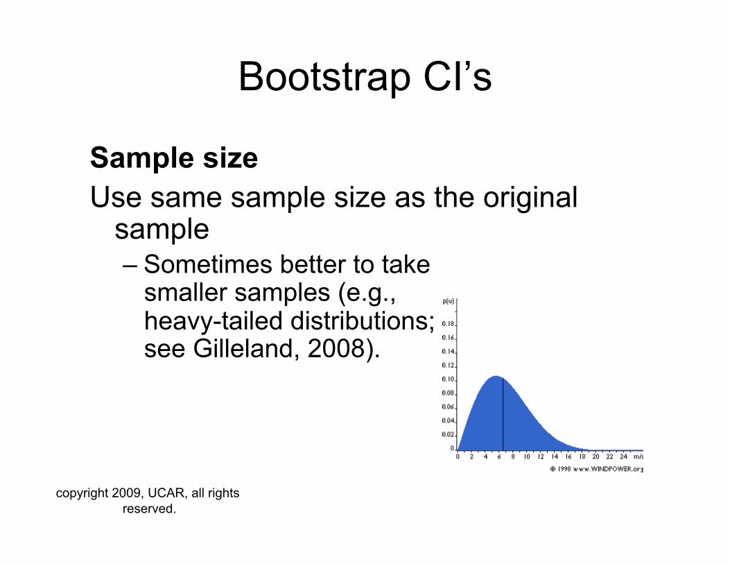
Bootstrap CI’s

Sample size Use same sample size as the original

sample – Sometimes better to take

smaller samples (e.g., heavy-tailed distributions; see Gilleland, 2008).


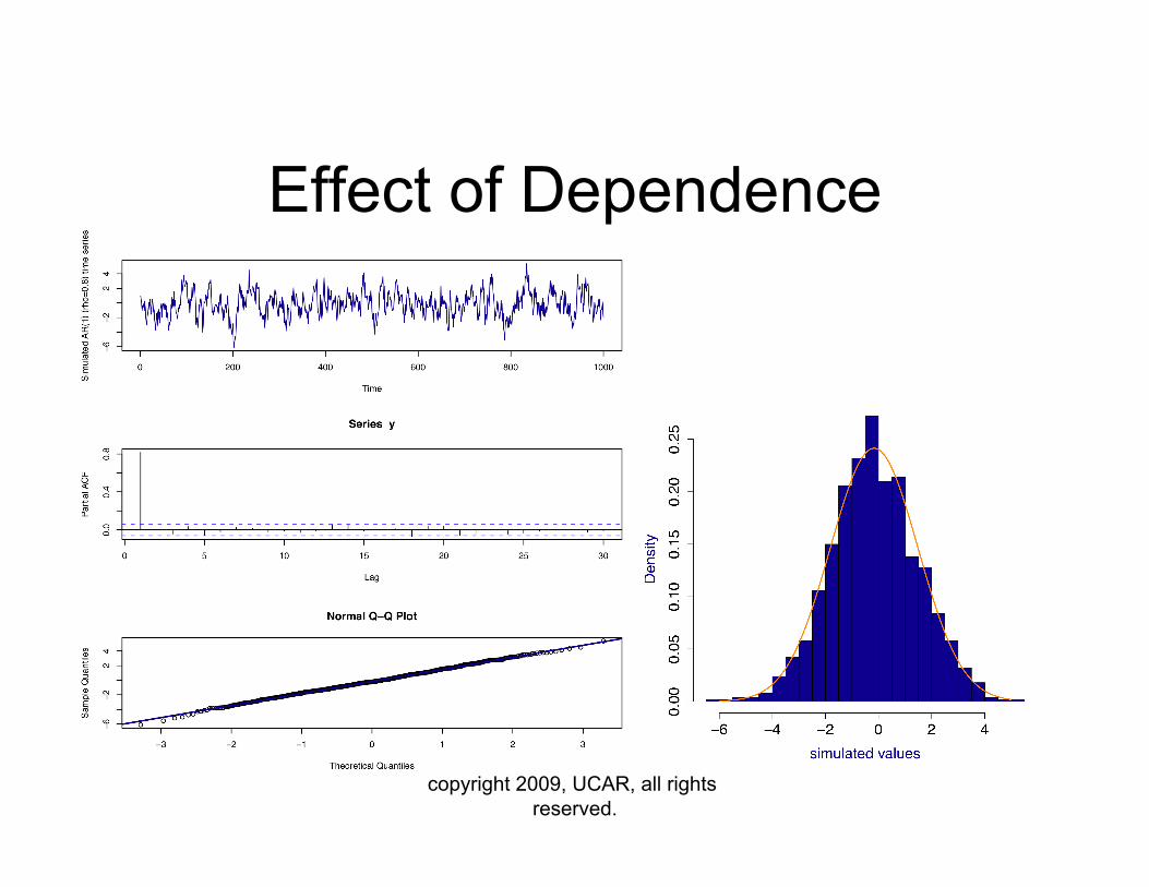
Effect of Dependence



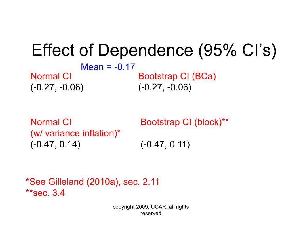
Effect of Dependence (95% CI’s) Normal CI (-0.27, -0.06)

Normal CI (w/ variance inflation)* (-0.47, 0.14)

*See Gilleland (2010a), sec. 2.11 **sec. 3.4

Bootstrap CI (BCa) (-0.27, -0.06)

Bootstrap CI (block)**

(-0.47, 0.11)

Mean = -0.17

Bootstrapping in R


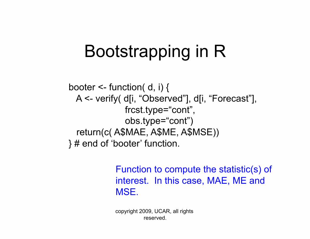
booter <- function( d, i) { A <- verify( d[i, “Observed”], d[i, “Forecast”],

frcst.type=“cont”, obs.type=“cont”)

return(c( A$MAE, A$ME, A$MSE)) } # end of ‘booter’ function.

Function to compute the statistic(s) of interest. In this case, MAE, ME and MSE.


Bootstrapping in R

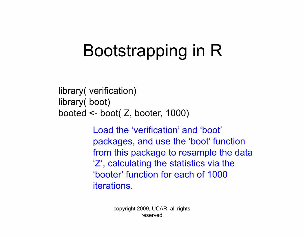
library( verification) library( boot) booted <- boot( Z, booter, 1000)

Load the ‘verification’ and ‘boot’ packages, and use the ‘boot’ function from this package to resample the data ‘Z’, calculating the statistics via the ‘booter’ function for each of 1000 iterations.


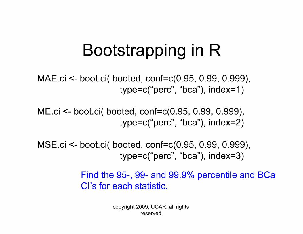
Bootstrapping in R MAE.ci <- boot.ci( booted, conf=c(0.95, 0.99, 0.999),

type=c(“perc”, “bca”), index=1)

ME.ci <- boot.ci( booted, conf=c(0.95, 0.99, 0.999), type=c(“perc”, “bca”), index=2)

MSE.ci <- boot.ci( booted, conf=c(0.95, 0.99, 0.999), type=c(“perc”, “bca”), index=3)

Find the 95-, 99- and 99.9% percentile and BCa CI’s for each statistic.


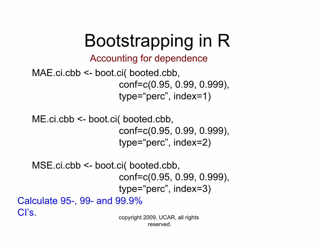
Bootstrapping in R Accounting for dependence

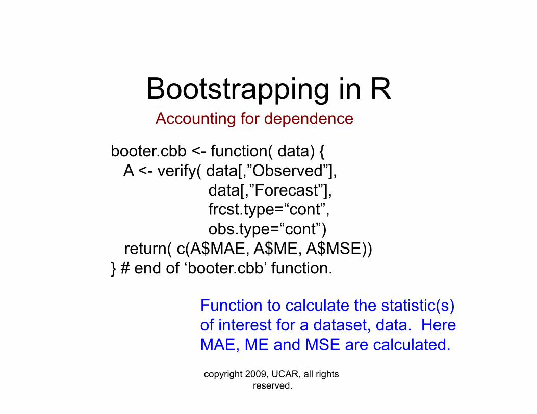
booter.cbb <- function( data) { A <- verify( data[,”Observed”],

data[,”Forecast”], frcst.type=“cont”, obs.type=“cont”)

return( c(A$MAE, A$ME, A$MSE)) } # end of ‘booter.cbb’ function.

Function to calculate the statistic(s) of interest for a dataset, data. Here MAE, ME and MSE are calculated.



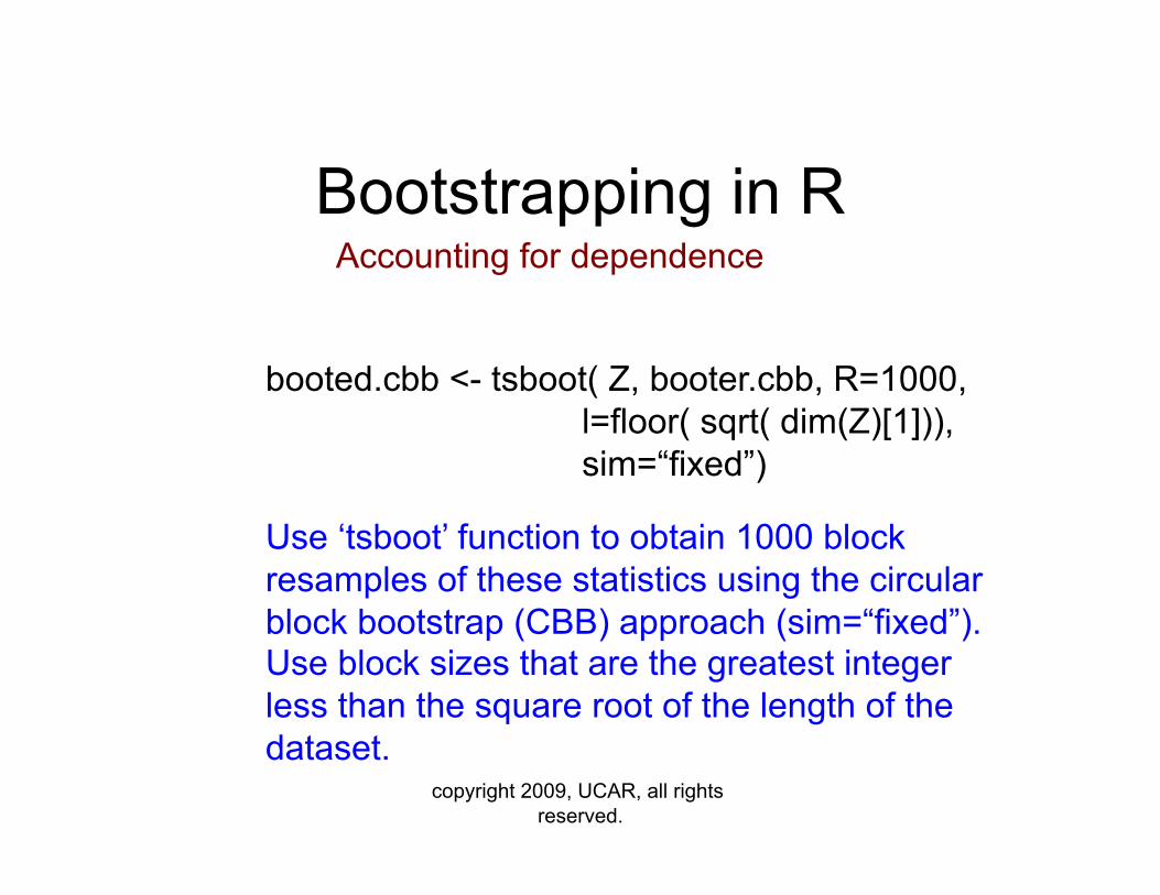
booted.cbb <- tsboot( Z, booter.cbb, R=1000, l=floor( sqrt( dim(Z)[1])), sim=“fixed”)

Use ‘tsboot’ function to obtain 1000 block resamples of these statistics using the circular block bootstrap (CBB) approach (sim=“fixed”). Use block sizes that are the greatest integer less than the square root of the length of the dataset.



Calculate 95-, 99- and 99.9% CI’s.

MAE.ci.cbb <- boot.ci( booted.cbb, conf=c(0.95, 0.99, 0.999), type=“perc”, index=1)

ME.ci.cbb <- boot.ci( booted.cbb, conf=c(0.95, 0.99, 0.999), type=“perc”, index=2)

MSE.ci.cbb <- boot.ci( booted.cbb, conf=c(0.95, 0.99, 0.999), type=“perc”, index=3)


Thank you. Questions? References

Gilleland, E., 2010a: Confidence intervals for forecast verification. NCAR Technical Note NCAR/TN-479+STR, 71pp. Available at:

http://nldr.library.ucar.edu/collections/technotes/asset-000-000-000-846.pdf

Gilleland, E., 2010b: Confidence intervals for forecast verification: Practical considerations, (unpublished manuscript, available at: http://www.ral.ucar.edu/staff/ericg/Gilleland2010.pdf)

Confidence Intervals - University Corporation for ...ericg/GillelandCItalkVxColloquium2010.pdf ·...

Documents

Transcript of Confidence Intervals - University Corporation for ...ericg/GillelandCItalkVxColloquium2010.pdf ·...