
Confidence Intervals CHAPTER SIX. Confidence Intervals for the MEAN (Large Samples) Section 6.1.
date post
21-Dec-2015Category
view
215download
1
Class 10: Tuesday, Oct. 12
• Hurricane data set, review of confidence intervals and hypothesis tests
• Confidence intervals for mean response• Prediction intervals• Transformations• Upcoming:
– Thursday: Finish transformations, Example Regression Analysis
– Tuesday: Review for midterm– Thursday: Midterm– Fall Break!

Hurricane Data • Is there a trend in the number of
hurricanes in the Atlantic over time (possibly an increase because of global warming)?
• hurricane.JMP contains data on the number of hurricanes in the Atlantic basin from 1950-1997.
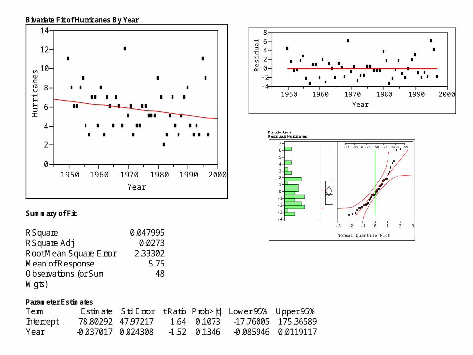
Bivariate Fit of Hurricanes By Year
0
2
4
6
8
10
12
14H
urric
anes
1950 1960 1970 1980 1990 2000
Year
Summary of Fit RSquare 0.047995 RSquare Adj 0.0273 Root Mean Square Error 2.33302 Mean of Response 5.75 Observations (or Sum Wgts)
48
Parameter Estimates Term Estimate Std Error t Ratio Prob>|t| Lower 95% Upper 95% Intercept 78.80292 47.97217 1.64 0.1073 -17.76005 175.36589 Year -0.037017 0.024308 -1.52 0.1346 -0.085946 0.0119117
-4-202468
Res
idua
l
1950 1960 1970 1980 1990 2000
Year
Distributions Residuals Hurricanes
-4
-3
-2
-1
0
1
2
3
4
5
6
7.01 .05 .10 .25 .50 .75 .90 .95 .99
-3 -2 -1 0 1 2 3
Normal Quantile Plot

Inferences for Hurricane Data
• Residual plots and normal quantile plots indicate that assumptions of linearity, constant variance and normality in simple linear regression model are reasonable.
• 95% confidence interval for slope (change in mean hurricanes between year t and year t+1): (-0.086,0.012)
• Hypothesis Test of null hypothesis that slope equals zero: test statistic = -1.52, p-value =0.13. We accept since p-value > 0.05. No evidence of a trend in hurricanes from 1950-1997.
0: 10 H
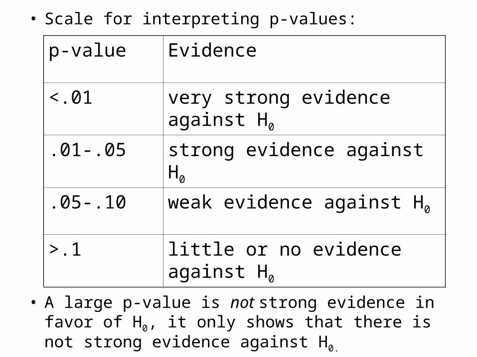
• Scale for interpreting p-values:
• A large p-value is not strong evidence in favor of H0, it only shows that there is not strong evidence against H0.
p-value Evidence
<.01 very strong evidence against H0
.01-.05 strong evidence against H0
.05-.10 weak evidence against H0
>.1 little or no evidence against H0
Inference in Regression
• Confidence intervals for slope
• Hypothesis test for slope
• Confidence intervals for mean response
• Prediction intervals

Car Price Example
• A used-car dealer wants to understand how odometer reading affects the selling price of used cars.
• The dealer randomly selects 100 three-year old Ford Tauruses that were sold at auction during the past month. Each car was in top condition and equipped with automatic transmission, AM/FM cassette tape player and air conditioning.
• carprices.JMP contains the price and number of miles on the odometer of each car.

Bivariate Fit of Price By Odometer
13500
14000
14500
15000
15500
16000P
rice
15000 25000 30000 35000 40000 45000
Odometer
Linear Fit Price = 17066.766 - 0.0623155 Odometer
Summary of Fit RSquare 0.650132 RSquare Adj 0.646562 Root Mean Square Error 303.1375 Mean of Response 14822.82 Observations (or Sum Wgts)
100
Parameter Estimates Term Estimate Std Error t Ratio Prob>|t| Lower 95% Upper 95% Intercept 17066.766 169.0246 100.97 <.0001 16731.342 17402.19 Odometer -0.062315 0.004618 -13.49 <.0001 -0.071479 -0.053152

• The used-car dealer has an opportunity to bid on a lot of cars offered by a rental company. The rental company has 250 Ford Tauruses, all equipped with automatic transmission, air conditioning and AM/FM cassette tape players. All of the cars in this lot have about 40,000 miles on the odometer. The dealer would like an estimate of the average selling price of all cars of this type with 40,000 miles on the odometer, i.e., E(Y|X=40,000).
• The least squares estimate is 575,14$40000*0623.017067)40000|(ˆ XYE

Confidence Interval for Mean Response
• Confidence interval for E(Y|X=40,000): A range of plausible values for E(Y|X=40,000) based on the sample.
• Approximate 95% Confidence interval:
• Notes about formula for SE: Standard error becomes smaller as sample size n increases, standard error is smaller the closer is to
• In JMP, after Fit Line, click red triangle next to Linear Fit and click Confid Curves Fit. Use the crosshair tool by clicking Tools, Crosshair to find the exact values of the confidence interval endpoints for a given X0.
)}|(ˆ{*2)|(ˆ00 XXYESEXXYE
n
i i XX
XX
nRMSEXXYESE
1
2
20
0)(
)(1)}|(ˆ{
0XX

Bivariate Fit of Price By Odometer
13500
14000
14500
15000
15500
16000P
rice
15000 25000 30000 35000 40000 45000
Odometer
Approximate 95% confidence interval for )000,40|(ˆ XYE ($14,514, $14,653)
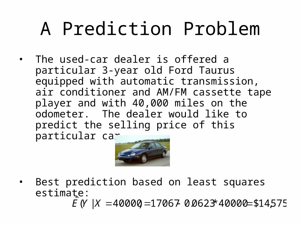
A Prediction Problem
• The used-car dealer is offered a particular 3-year old Ford Taurus equipped with automatic transmission, air conditioner and AM/FM cassette tape player and with 40,000 miles on the odometer. The dealer would like to predict the selling price of this particular car.
• Best prediction based on least squares estimate:
575,14$40000*0623.017067)40000|(ˆ XYE

Range of Selling Prices for Particular Car
• The dealer is interested in the range of selling prices that this particular car with 40,000 miles on it is likely to have.
• Under simple linear regression model, Y|X follows a normal distribution with mean and standard deviation . A car with 40,000 miles on it will be in interval about 95% of the time.
• Class 5: We substituted the least squares estimates for for and said car with 40,000 miles on it will be in interval about 95% of the time. This is a good approximation but it ignores potential error in least square estimates.
X*10
*240000*10
RMSE,ˆ,ˆ10 ,, 10
RMSE*240000*ˆˆ10

Prediction Interval
• 95% Prediction Interval: An interval that has approximately a 95% chance of containing the value of Y for a particular unit with X=X0 ,where the particular unit is not in the original sample.
• Approximate 95% prediction interval:
• In JMP, after Fit Line, click red triangle next to Linear Fit and click Confid Curves Indiv. Use the crosshair tool by clicking Tools, Crosshair to find the exact values of the prediction interval endpoints for a given X0.
n
i i XXn
RMSEXXYE1
20 )(
11*2)|(ˆ

B i v a r i a t e F i t o f P r i c e B y O d o m e t e r
13500
14000
14500
15000
15500
16000Price
15000 30000 40000Odometer
9 5 % C o n f i d e n c e I n t e r v a l f o r )14653 ,14514( }40000|{ XY 9 5 % P r e d i c t i o n I n t e r v a l f o r X = 4 0 0 0 0 15194) ,13972(
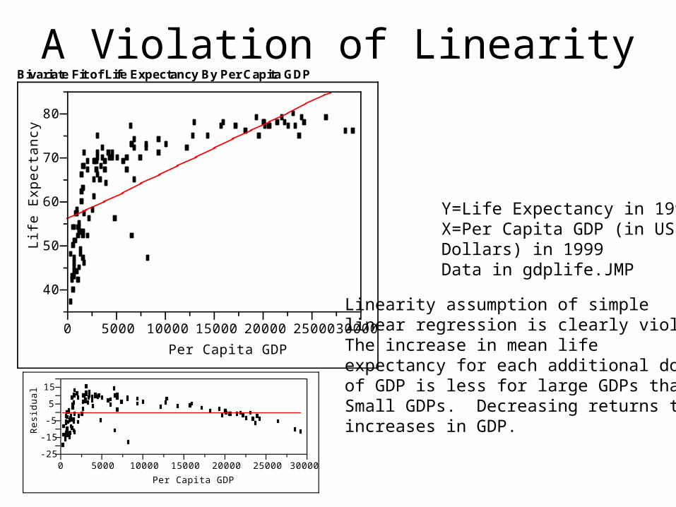
A Violation of LinearityBivariate Fit of Life Expectancy By Per Capita GDP
40
50
60
70
80
Life
Exp
ecta
ncy
0 5000 10000 15000 20000 25000 30000
Per Capita GDP
-25
-15
-5
5
15
Res
idua
l
0 5000 10000 15000 20000 25000 30000
Per Capita GDP
Y=Life Expectancy in 1999X=Per Capita GDP (in US Dollars) in 1999Data in gdplife.JMP
Linearity assumption of simplelinear regression is clearly violated.The increase in mean life expectancy for each additional dollarof GDP is less for large GDPs thanSmall GDPs. Decreasing returns toincreases in GDP.

Transformations
• Violation of linearity: E(Y|X) is not a straight line.
• Transformations: Perhaps E(f(Y)|g(X)) is a straight line, where f(Y) and g(X) are transformations of Y and X, and a simple linear regression model holds for the response variable f(Y) and explanatory variable g(X).

Bivariate Fit of Life Expectancy By log Per Capita GDP
40
50
60
70
80
Life
Exp
ecta
ncy
6 7 8 9 10
log Per Capita GDP
Linear Fit Life Expectancy = -7.97718 + 8.729051 log Per Capita GDP
-25
-15
-5
5
15
Res
idua
l
6 7 8 9 10
log Per Capita GDP
The mean of Life Expectancy | Log Per Capita appears to be approximatelya straight line.

How do we use the transformation?
•
• Testing for association between Y and X: If the simple linear regression model holds for f(Y) and g(X), then Y and X are associated if and only if the slope in the regression of f(Y) and g(X) does not equal zero. P-value for test that slope is zero is <.0001: Strong evidence that per capita GDP and life expectancy are associated.
• Prediction and mean response: What would you predict the life expectancy to be for a country with a per capita GDP of $20,000?
Linear Fit Life Expectancy = -7.97718 + 8.729051 log Per Capita GDP Parameter Estimates Term Estimate Std Error t Ratio Prob>|t| Intercept -7.97718 3.943378 -2.02 0.0454 log Per Capita GDP
8.729051 0.474257 18.41 <.0001
47.789035.9*7291.89772.7)9035.9log|(ˆ
)000,20loglog|(ˆ)000,20|(ˆ
XYE
XYEXYE

How do we choose a transformation?
• Tukey’s Bulging Rule.
• See Handout.
• Match curvature in data to the shape of one of the curves drawn in the four quadrants of the figure in the handout. Then use the associated transformations, selecting one for either X, Y or both.

Transformations in JMP1. Use Tukey’s Bulging rule (see handout) to determine
transformations which might help. 2. After Fit Y by X, click red triangle next to Bivariate Fit and click Fit
Special. Experiment with transformations suggested by Tukey’s Bulging rule.
3. Make residual plots of the residuals for transformed model vs. the original X by clicking red triangle next to Transformed Fit to … and clicking plot residuals. Choose transformations which make the residual plot have no pattern in the mean of the residuals vs. X.
4. Compare different transformations by looking for transformation with smallest root mean square error on original y-scale. If using a transformation that involves transforming y, look at root mean square error for fit measured on original scale.

Bivariate Fit of Life Expectancy By Per Capita GDP
40
50
60
70
80Li
fe E
xpec
tanc
y
0 5000 10000 15000 20000 25000 30000
Per Capita GDP
Linear Fit
Transformed Fit to Log
Transformed Fit to Sqrt
Transformed Fit Square
`
•
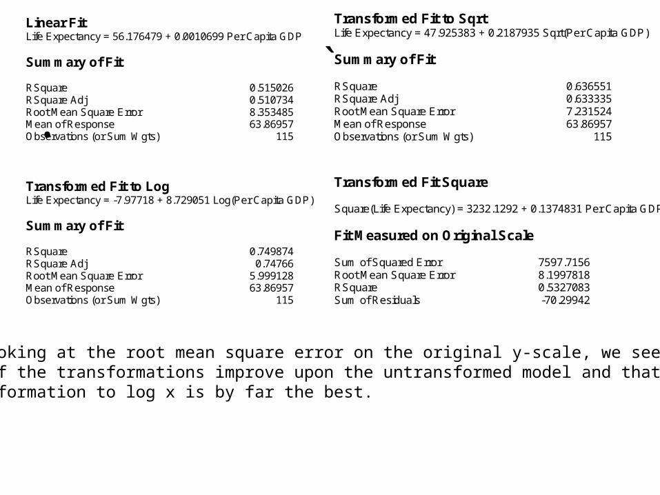
Linear Fit Life Expectancy = 56.176479 + 0.0010699 Per Capita GDP Summary of Fit RSquare 0.515026 RSquare Adj 0.510734 Root Mean Square Error 8.353485 Mean of Response 63.86957 Observations (or Sum Wgts) 115 Transformed Fit to Log Life Expectancy = -7.97718 + 8.729051 Log(Per Capita GDP) Summary of Fit RSquare 0.749874 RSquare Adj 0.74766 Root Mean Square Error 5.999128 Mean of Response 63.86957 Observations (or Sum Wgts) 115
Transformed Fit to Sqrt Life Expectancy = 47.925383 + 0.2187935 Sqrt(Per Capita GDP) Summary of Fit RSquare 0.636551 RSquare Adj 0.633335 Root Mean Square Error 7.231524 Mean of Response 63.86957 Observations (or Sum Wgts) 115 Transformed Fit Square Square(Life Expectancy) = 3232.1292 + 0.1374831 Per Capita GDP Fit Measured on Original Scale Sum of Squared Error 7597.7156 Root Mean Square Error 8.1997818 RSquare 0.5327083 Sum of Residuals -70.29942
By looking at the root mean square error on the original y-scale, we see thatall of the transformations improve upon the untransformed model and that the transformation to log x is by far the best.

Linear Fit
-25
-15
-5
5
15
Res
idua
l
0 5000 10000 15000 20000 25000 30000
Per Capita GDP
Transformation to Log X
-25
-15
-5
5
15
Res
idua
l
0 5000 10000 15000 20000 25000 30000
Per Capita GDP
Transformation to X
-25
-15
-5
5
15
Res
idua
l
0 5000 10000 15000 20000 25000 30000
Per Capita GDP
Transformation to 2Y
-25
-15
-5
5
15
Res
idua
l
0 5000 10000 15000 20000 25000 30000
Per Capita GDP
The transformation to Log X appears to have mostly removed a trend in the meanof the residuals. This means that . There is still a problem of nonconstant variance.
XXYE log)|( 10