Tutorial - Basic GeoTIFF manipulation using ILWIS 1.1 ... - ILWIS... · 6/1/2015 · Tutorial -...
20
© INPE - National Institute for Space Research - Brazil - 2015 1 Tutorial - Basic GeoTIFF manipulation using ILWIS 1 - Getting Ready 1.1 Software Download and Installation: Download the ILWIS software at the following link: http://52north.org/downloads/category/135-ilwis-3-08-04- package, and extract the executable file “setup.exe” in your local directory. Figure 1: ILWIS download webpage Follow the standard Windows installation procedure (Next -> Install). After installing it with the standard options, the software directory will be located at “C:\Program Files (x86)\n52\ILWIS38”. 1.2 Download the tutorial images: Download the tutorial GeoTIFF images at the following link: ftp://server-ftpdsa.cptec.inpe.br/Basic_GeoTIFF/ username: geonetcast password: GNC-A Create a folder called “VLAB” in the “C:\” directory and extract the compressed GeoTIFF files in it. From now on this folder will be referred as “work folder” in this tutorial. Hint: The GeoTIFF imagery like the ones used in this tutorial are broadcasted in near real-time through the GEONETCast-Americas system and may be found at “KenCast\Fazzt\incoming\NOAA-NESDIS-GEOTIFFS\IMAGERY” and at “KenCast\Fazzt\incoming\INPE” in your local receive station.
Transcript of Tutorial - Basic GeoTIFF manipulation using ILWIS 1.1 ... - ILWIS... · 6/1/2015 · Tutorial -...
© INPE - National Institute for Space Research - Brazil - 2015 1
Tutorial - Basic GeoTIFF manipulation using ILWIS
1 - Getting Ready
1.1 Software Download and Installation:
Download the ILWIS software at the following link: http://52north.org/downloads/category/135-ilwis-3-08-04-
package, and extract the executable file “setup.exe” in your local directory.
Figure 1: ILWIS download webpage
Follow the standard Windows installation procedure (Next -> Install). After installing it with the standard options, the
software directory will be located at “C:\Program Files (x86)\n52\ILWIS38”.
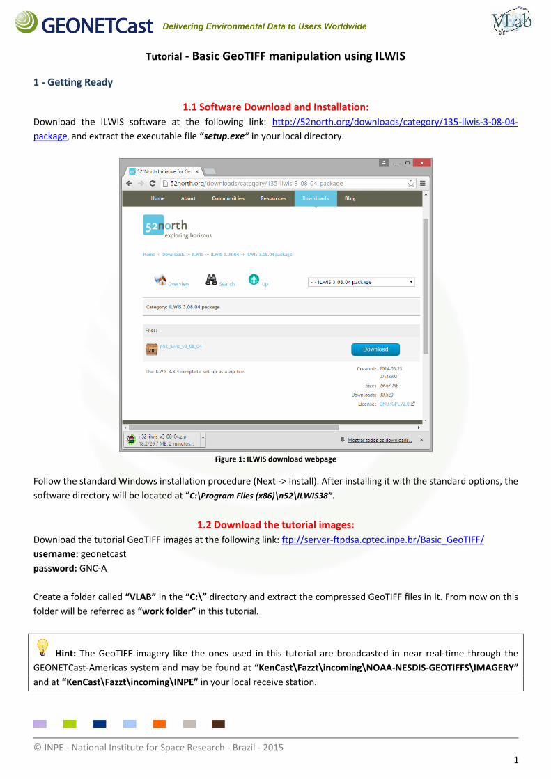
1.2 Download the tutorial images:
Download the tutorial GeoTIFF images at the following link: ftp://server-ftpdsa.cptec.inpe.br/Basic_GeoTIFF/
username: geonetcast
password: GNC-A
Create a folder called “VLAB” in the “C:\” directory and extract the compressed GeoTIFF files in it. From now on this
folder will be referred as “work folder” in this tutorial.
Hint: The GeoTIFF imagery like the ones used in this tutorial are broadcasted in near real-time through the
GEONETCast-Americas system and may be found at “KenCast\Fazzt\incoming\NOAA-NESDIS-GEOTIFFS\IMAGERY”
and at “KenCast\Fazzt\incoming\INPE” in your local receive station.
© INPE - National Institute for Space Research - Brazil - 2015 2
1.3 Download the tutorial color tables:
Download the tutorial color tables at the following link: ftp://server-ftpdsa.cptec.inpe.br/Color_Tables/
Extract the “Color_Tables.zip” file in the ILWIS “system” folder “C:\Program Files (x86)\n52\ILWIS38\system”.
2 – Manipulating the first GeoTIFF
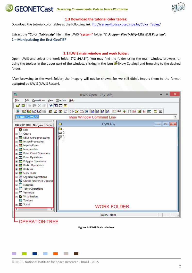
2.1 ILWIS main window and work folder:
Open ILWIS and select the work folder (“C:\VLAB”). You may find the folder using the main window browser, or
using the toolbar in the upper part of the window, clicking in the icon [New Catalog] and browsing to the desired
folder.
After browsing to the work folder, the imagery will not be shown, for we still didn’t import them to the format
accepted by ILWIS (ILWIS Raster).
Figure 2: ILWIS Main Window
© INPE - National Institute for Space Research - Brazil - 2015 3
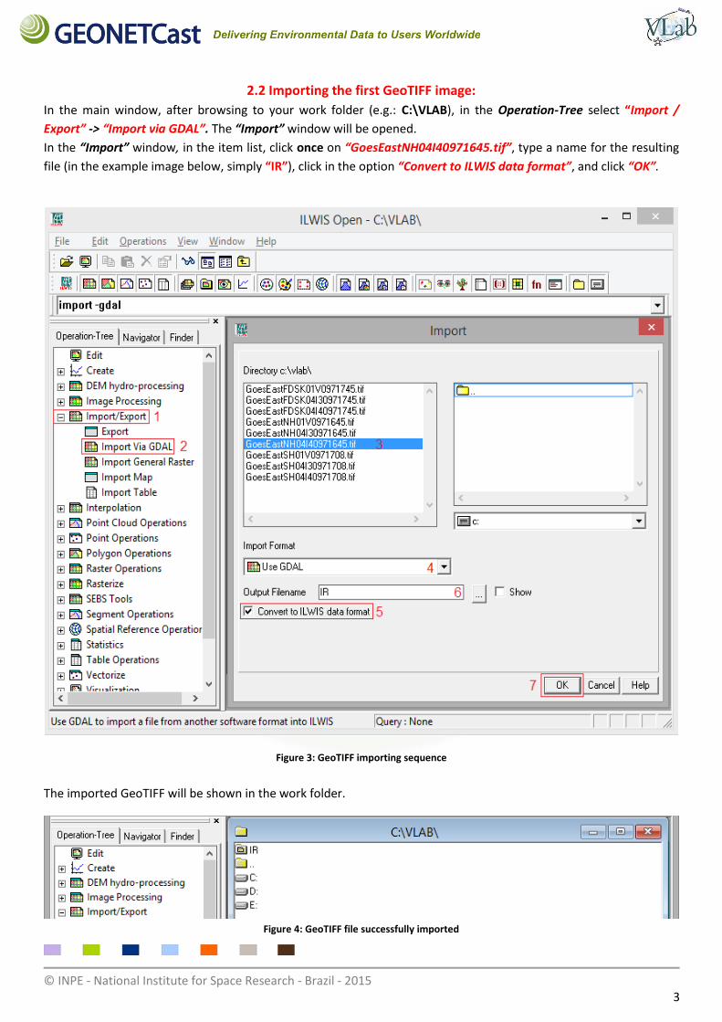
2.2 Importing the first GeoTIFF image:
In the main window, after browsing to your work folder (e.g.: C:\VLAB), in the Operation-Tree select “Import /
Export” -> “Import via GDAL”. The “Import” window will be opened.
In the “Import” window, in the item list, click once on “GoesEastNH04I40971645.tif”, type a name for the resulting
file (in the example image below, simply “IR”), click in the option “Convert to ILWIS data format”, and click “OK”.
Figure 3: GeoTIFF importing sequence
The imported GeoTIFF will be shown in the work folder.
Figure 4: GeoTIFF file successfully imported
© INPE - National Institute for Space Research - Brazil - 2015 4
Hint: ILWIS has a command line interface. In some cases, you may avoid using the graphical interface and type
commands in the main window command line to carry out operations, calculations and scripts. For example, to
import the GeoTIFF from the last step, you could have used the following command in the main window command
line:
open goeseastnh04i40971645.tif -import -output=IR -noshow -method=gdal
You can even call these instructions from an external script (e.g.: a DOS batch script)
From now on, the command line alternatives will be referenced with the following icon:
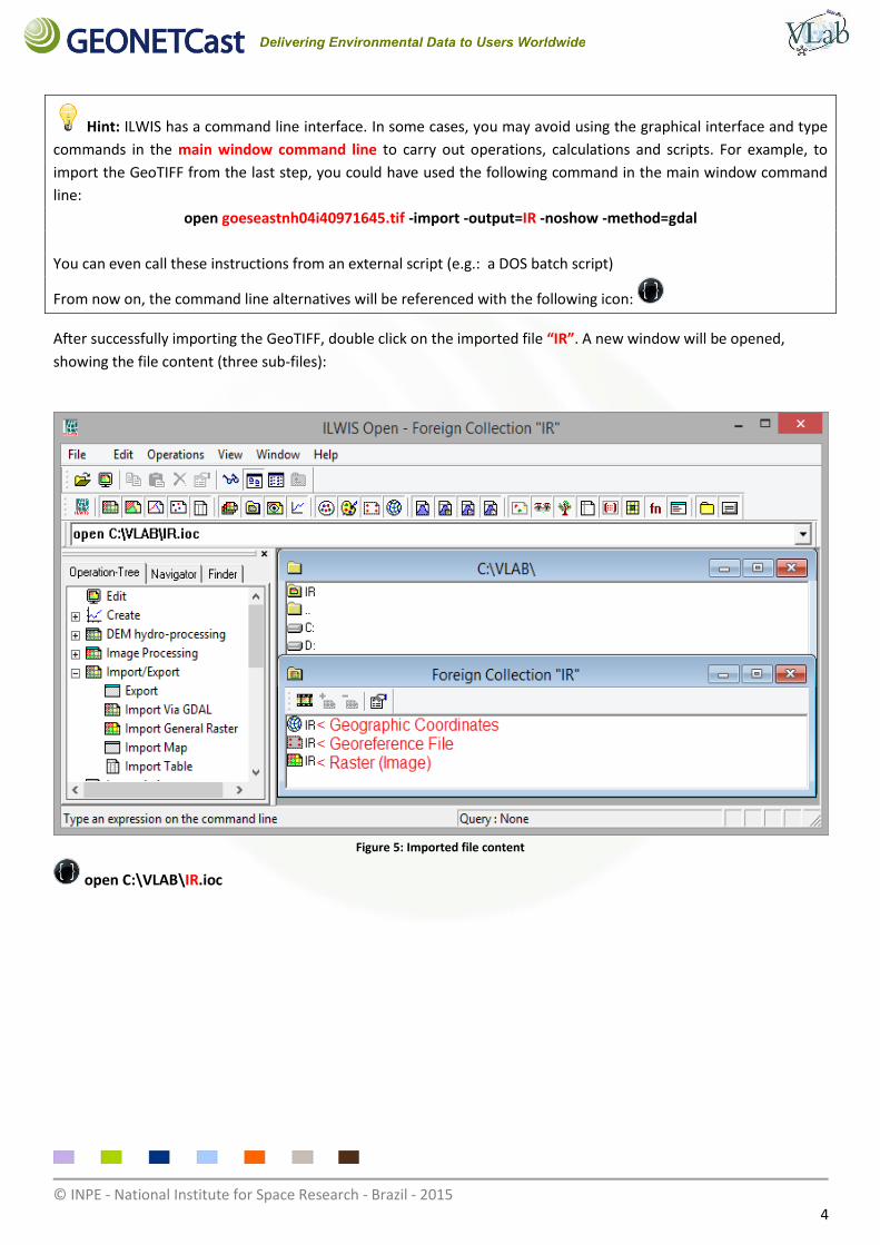
After successfully importing the GeoTIFF, double click on the imported file “IR”. A new window will be opened,
showing the file content (three sub-files):
Figure 5: Imported file content
open C:\VLAB\IR.ioc
© INPE - National Institute for Space Research - Brazil - 2015 5
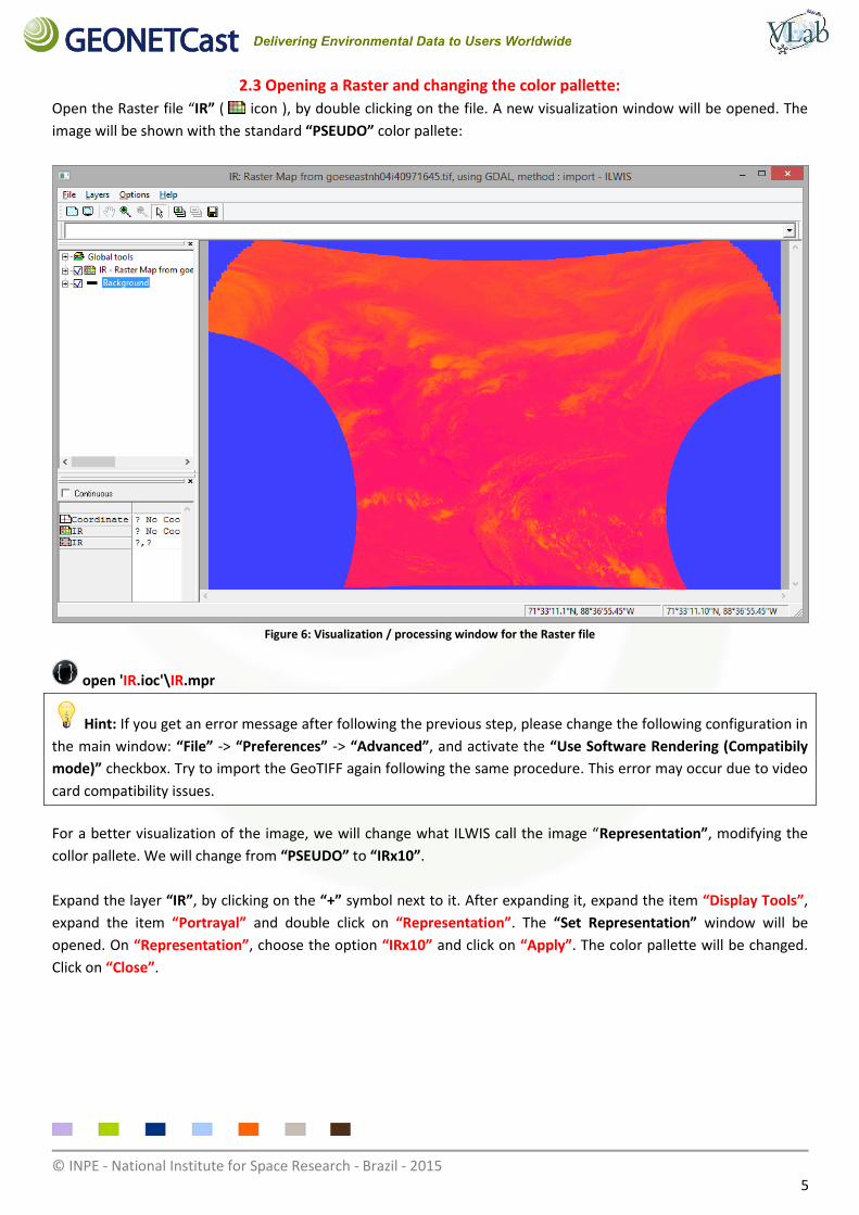
2.3 Opening a Raster and changing the color pallette:
Open the Raster file “IR” ( icon ), by double clicking on the file. A new visualization window will be opened. The
image will be shown with the standard “PSEUDO” color pallete:
Figure 6: Visualization / processing window for the Raster file
open 'IR.ioc'\IR.mpr
Hint: If you get an error message after following the previous step, please change the following configuration in
the main window: “File” -> “Preferences” -> “Advanced”, and activate the “Use Software Rendering (Compatibily
mode)” checkbox. Try to import the GeoTIFF again following the same procedure. This error may occur due to video
card compatibility issues.
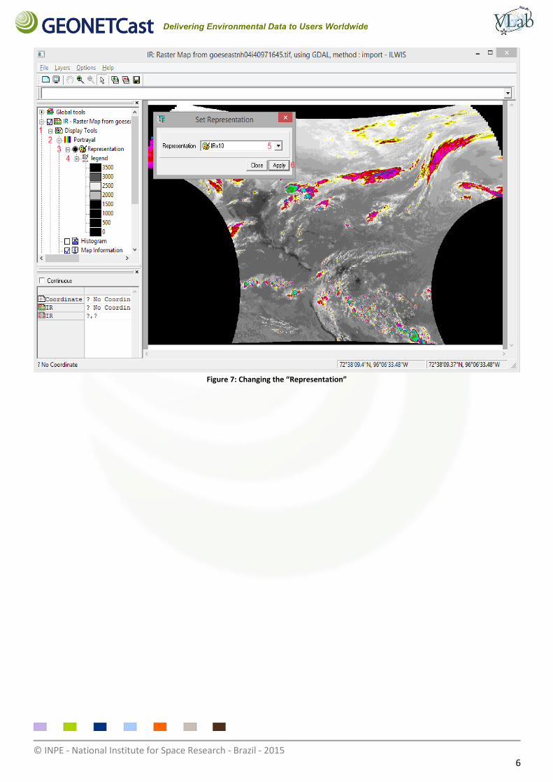
For a better visualization of the image, we will change what ILWIS call the image “Representation”, modifying the
collor pallete. We will change from “PSEUDO” to “IRx10”.
Expand the layer “IR”, by clicking on the “+” symbol next to it. After expanding it, expand the item “Display Tools”,
expand the item “Portrayal” and double click on “Representation”. The “Set Representation” window will be
opened. On “Representation”, choose the option “IRx10” and click on “Apply”. The color pallette will be changed.
Click on “Close”.
© INPE - National Institute for Space Research - Brazil - 2015 6
Figure 7: Changing the “Representation”
© INPE - National Institute for Space Research - Brazil - 2015 7
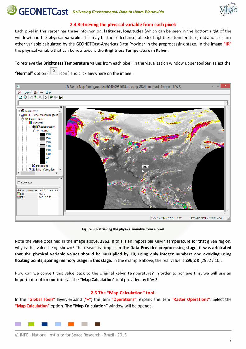
2.4 Retrieving the physical variable from each pixel:
Each pixel in this raster has three information: latitudes, longitudes (which can be seen in the bottom right of the
window) and the physical variable. This may be the reflectance, albedo, brightness temperature, radiation, or any
other variable calculated by the GEONETCast-Americas Data Provider in the preprocessing stage. In the image "IR"
the physical variable that can be retrieved is the Brightness Temperature in Kelvin.
To retrieve the Brightness Temperature values from each pixel, in the visualization window upper toolbar, select the
“Normal” option ( icon ) and click anywhere on the image.
Figure 8: Retrieving the physical variable from a pixel
Note the value obtained in the image above, 2962. If this is an impossible Kelvin temperature for that given region,
why is this value being shown? The reason is simple: In the Data Provider preprocessing stage, it was arbitrated
that the physical variable values should be multiplied by 10, using only integer numbers and avoiding using
floating points, sparing memory usage in this stage. In the example above, the real value is 296,2 K (2962 / 10).
How can we convert this value back to the original kelvin temperature? In order to achieve this, we will use an
important tool for our tutorial, the “Map Calculation” tool provided by ILWIS.
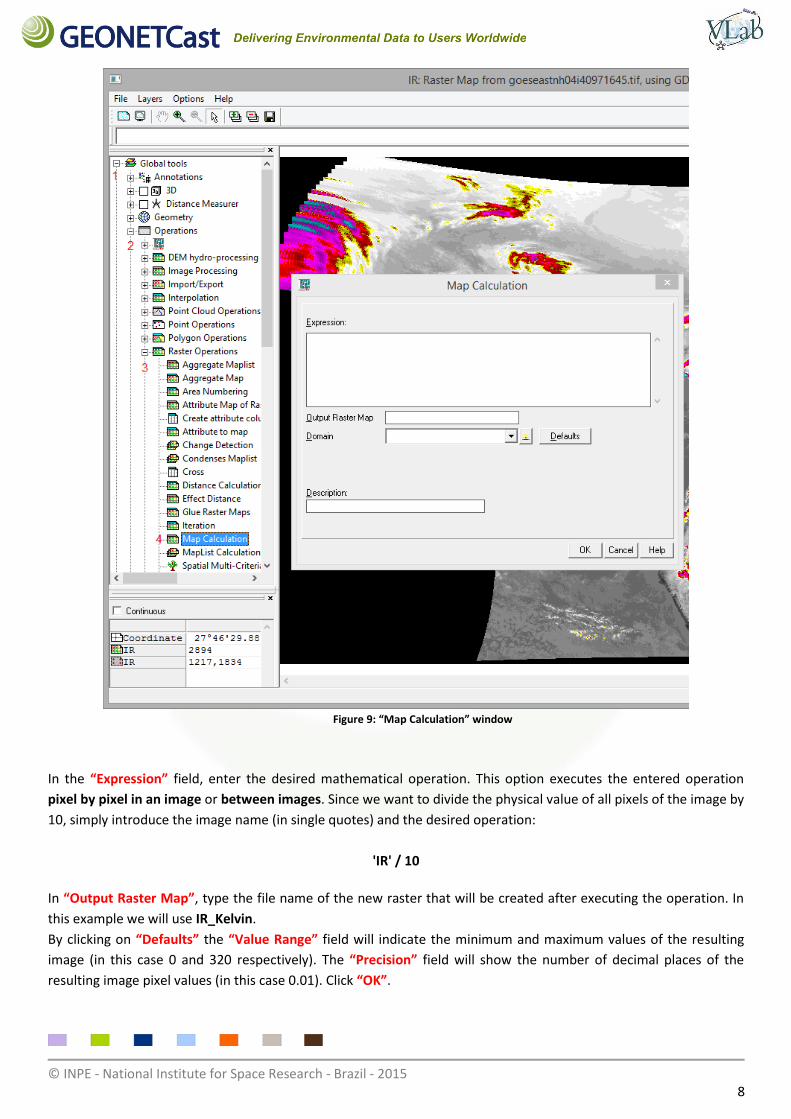
2.5 The “Map Calculation” tool:
In the “Global Tools” layer, expand (“+”) the item “Operations”, expand the item “Raster Operations”. Select the
“Map Calculation” option. The “Map Calculation” window will be opened.
© INPE - National Institute for Space Research - Brazil - 2015 8
Figure 9: “Map Calculation” window
In the “Expression” field, enter the desired mathematical operation. This option executes the entered operation
pixel by pixel in an image or between images. Since we want to divide the physical value of all pixels of the image by
10, simply introduce the image name (in single quotes) and the desired operation:
'IR' / 10
In “Output Raster Map”, type the file name of the new raster that will be created after executing the operation. In
this example we will use IR_Kelvin.
By clicking on “Defaults” the “Value Range” field will indicate the minimum and maximum values of the resulting
image (in this case 0 and 320 respectively). The “Precision” field will show the number of decimal places of the
resulting image pixel values (in this case 0.01). Click “OK”.
© INPE - National Institute for Space Research - Brazil - 2015 9
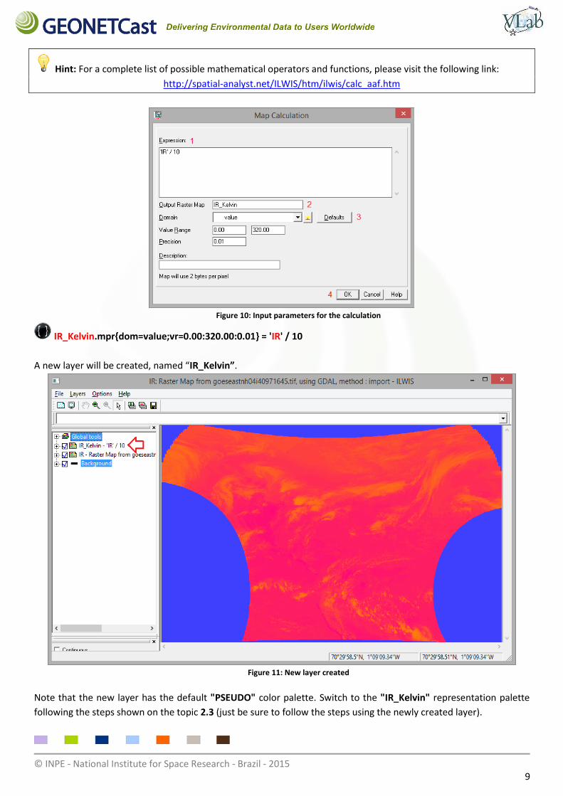
Hint: For a complete list of possible mathematical operators and functions, please visit the following link:
http://spatial-analyst.net/ILWIS/htm/ilwis/calc_aaf.htm
Figure 10: Input parameters for the calculation
IR_Kelvin.mpr{dom=value;vr=0.00:320.00:0.01} = 'IR' / 10
A new layer will be created, named “IR_Kelvin”.
Figure 11: New layer created
Note that the new layer has the default "PSEUDO" color palette. Switch to the "IR_Kelvin" representation palette
following the steps shown on the topic 2.3 (just be sure to follow the steps using the newly created layer).
© INPE - National Institute for Space Research - Brazil - 2015 10
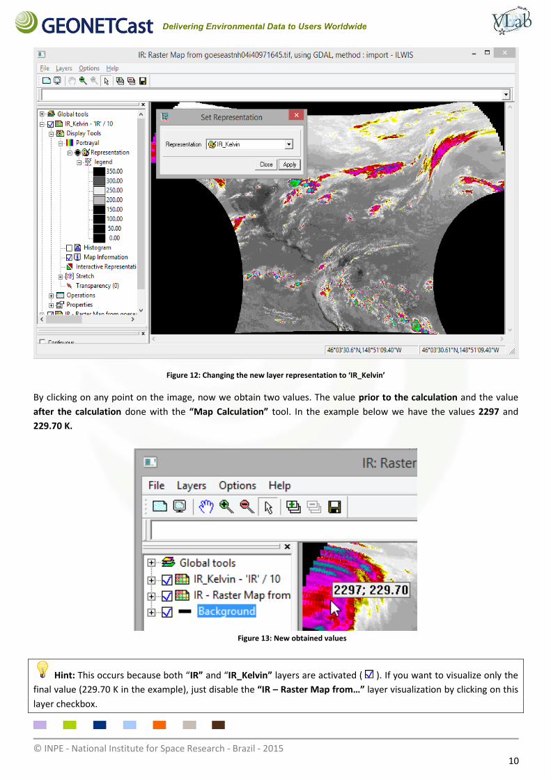
Figure 12: Changing the new layer representation to ‘IR_Kelvin’
By clicking on any point on the image, now we obtain two values. The value prior to the calculation and the value
after the calculation done with the “Map Calculation” tool. In the example below we have the values 2297 and
229.70 K.
Figure 13: New obtained values
Hint: This occurs because both “IR” and “IR_Kelvin” layers are activated ( ). If you want to visualize only the
final value (229.70 K in the example), just disable the “IR – Raster Map from…” layer visualization by clicking on this
layer checkbox.
© INPE - National Institute for Space Research - Brazil - 2015 11
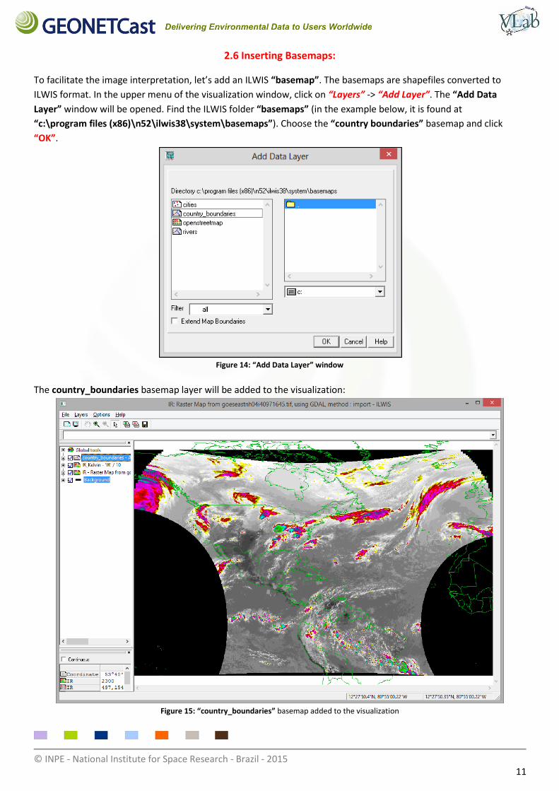
2.6 Inserting Basemaps:
To facilitate the image interpretation, let’s add an ILWIS “basemap”. The basemaps are shapefiles converted to
ILWIS format. In the upper menu of the visualization window, click on “Layers” -> “Add Layer”. The “Add Data
Layer” window will be opened. Find the ILWIS folder “basemaps” (in the example below, it is found at
“c:\program files (x86)\n52\ilwis38\system\basemaps”). Choose the “country boundaries” basemap and click
“OK”.
Figure 14: “Add Data Layer” window
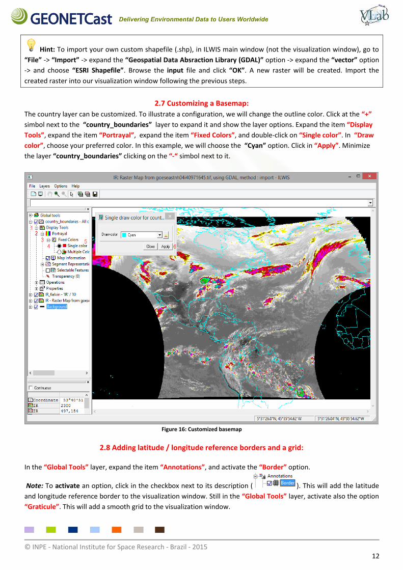
The country_boundaries basemap layer will be added to the visualization:
Figure 15: “country_boundaries” basemap added to the visualization
© INPE - National Institute for Space Research - Brazil - 2015 12
Hint: To import your own custom shapefile (.shp), in ILWIS main window (not the visualization window), go to
“File” -> “Import” -> expand the “Geospatial Data Absraction Library (GDAL)” option -> expand the “vector” option
-> and choose “ESRI Shapefile”. Browse the input file and click “OK”. A new raster will be created. Import the
created raster into our visualization window following the previous steps.
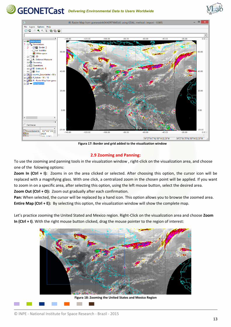
2.7 Customizing a Basemap:
The country layer can be customized. To illustrate a configuration, we will change the outline color. Click at the “+”
simbol next to the “country_boundaries” layer to expand it and show the layer options. Expand the item “Display
Tools”, expand the item “Portrayal”, expand the item “Fixed Colors”, and double-click on “Single color”. In “Draw
color”, choose your preferred color. In this example, we will choose the “Cyan” option. Click in “Apply”. Minimize
the layer “country_boundaries” clicking on the “-“ simbol next to it.
Figure 16: Customized basemap
2.8 Adding latitude / longitude reference borders and a grid:
In the “Global Tools” layer, expand the item “Annotations”, and activate the “Border” option.
Note: To activate an option, click in the checkbox next to its description ( ). This will add the latitude
and longitude reference border to the visualization window. Still in the “Global Tools” layer, activate also the option
“Graticule”. This will add a smooth grid to the visualization window.
© INPE - National Institute for Space Research - Brazil - 2015 13
Figura 17: Border and grid added to the visualization window
2.9 Zooming and Panning:
To use the zooming and panning tools in the visualzation window , right-click on the visualization area, and choose
one of the folowing options:
Zoom In (Ctrl + I): Zooms in on the area clicked or selected. After choosing this option, the cursor icon will be
replaced with a magnifying glass. With one click, a centralized zoom in the chosen point will be applied. If you want
to zoom in on a specific area, after selecting this option, using the left mouse button, select the desired area.
Zoom Out (Ctrl + O): Zoom out gradually after each confirmation.
Pan: When selected, the cursor will be replaced by a hand icon. This option allows you to browse the zoomed area.
Entire Map (Ctrl + E): By selecting this option, the visualization window will show the complete map.
Let’s practice zooming the United Stated and Mexico region. Right-Click on the visualization area and choose Zoom
In (Ctrl + I). With the right mouse button clicked, drag the mouse pointer to the region of interest:
Figura 18: Zooming the United States and Mexico Region
© INPE - National Institute for Space Research - Brazil - 2015 14
Figura 19: United States and Mexico region zoomed
Go back to the full map visualization right-clicling and choosing Entire Map or typing Ctrl + E.
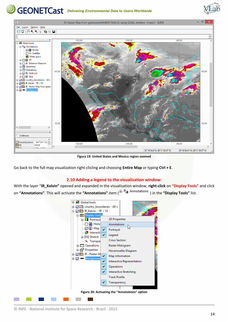
2.10 Adding a legend to the visualization window:
With the layer “IR_Kelvin” opened and expanded in the visualization window, right-click on “Display Tools” and click
on “Annotations”. This will activate the “Annotations” item ( ) in the “Display Tools” list.
Figure 20: Activating the “Annotations” option
© INPE - National Institute for Space Research - Brazil - 2015 15
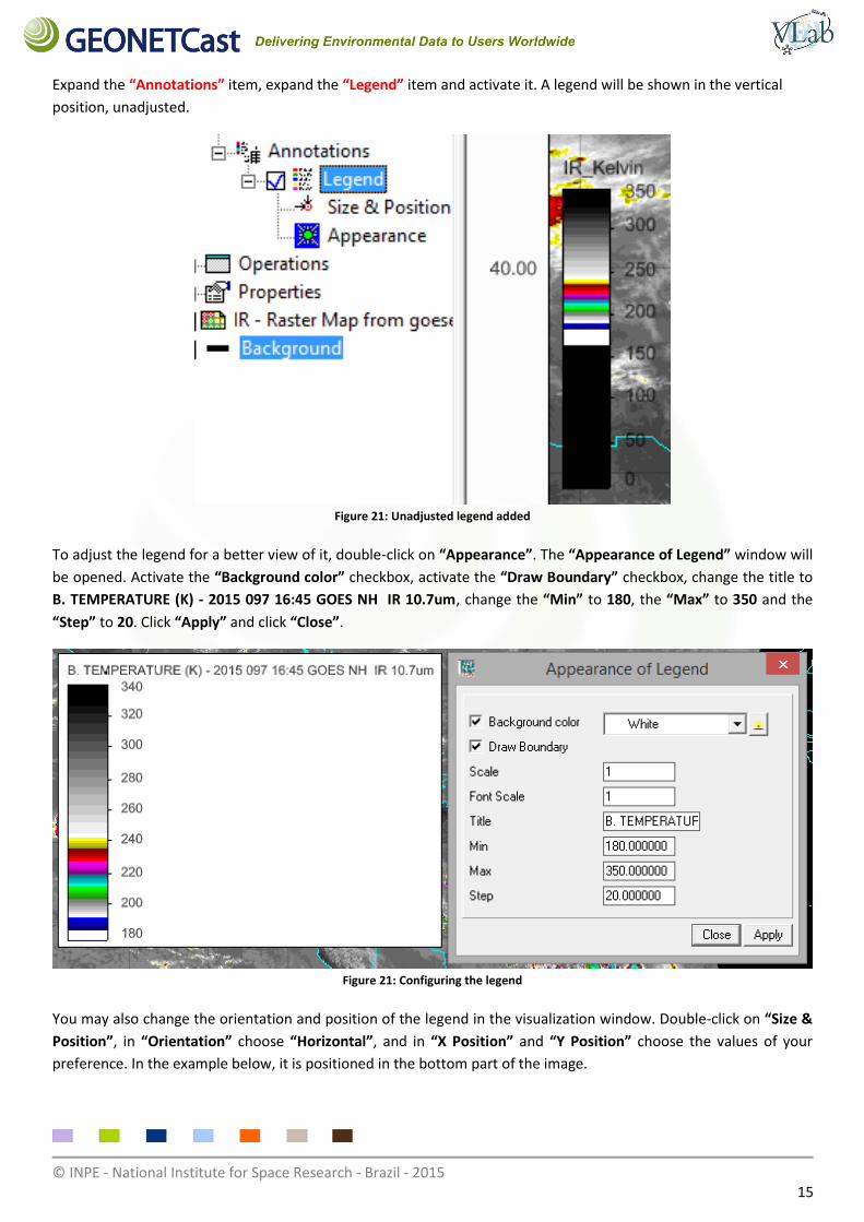
Expand the “Annotations” item, expand the “Legend” item and activate it. A legend will be shown in the vertical
position, unadjusted.
Figure 21: Unadjusted legend added
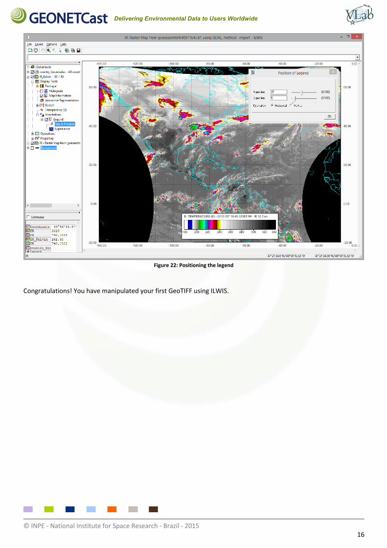
To adjust the legend for a better view of it, double-click on “Appearance”. The “Appearance of Legend” window will
be opened. Activate the “Background color” checkbox, activate the “Draw Boundary” checkbox, change the title to
B. TEMPERATURE (K) - 2015 097 16:45 GOES NH IR 10.7um, change the “Min” to 180, the “Max” to 350 and the
“Step” to 20. Click “Apply” and click “Close”.
Figure 21: Configuring the legend
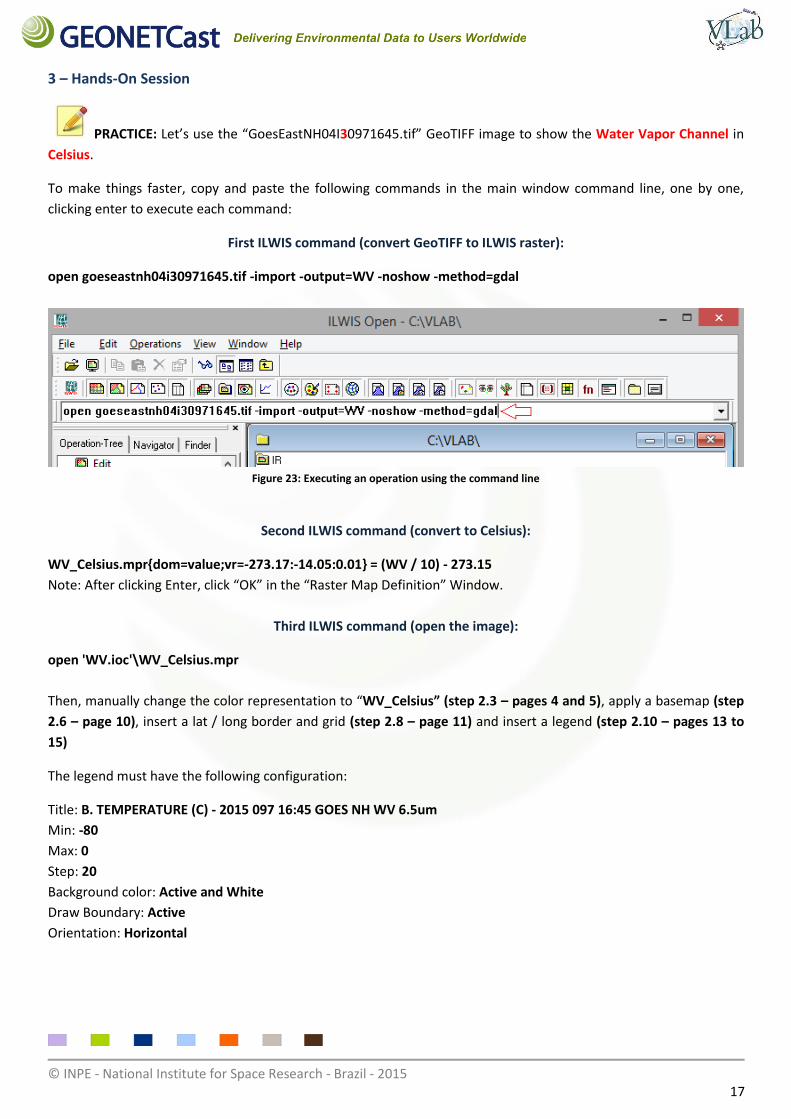
You may also change the orientation and position of the legend in the visualization window. Double-click on “Size &
Position”, in “Orientation” choose “Horizontal”, and in “X Position” and “Y Position” choose the values of your
preference. In the example below, it is positioned in the bottom part of the image.
© INPE - National Institute for Space Research - Brazil - 2015 16
Figure 22: Positioning the legend
Congratulations! You have manipulated your first GeoTIFF using ILWIS.
© INPE - National Institute for Space Research - Brazil - 2015 17
3 – Hands-On Session
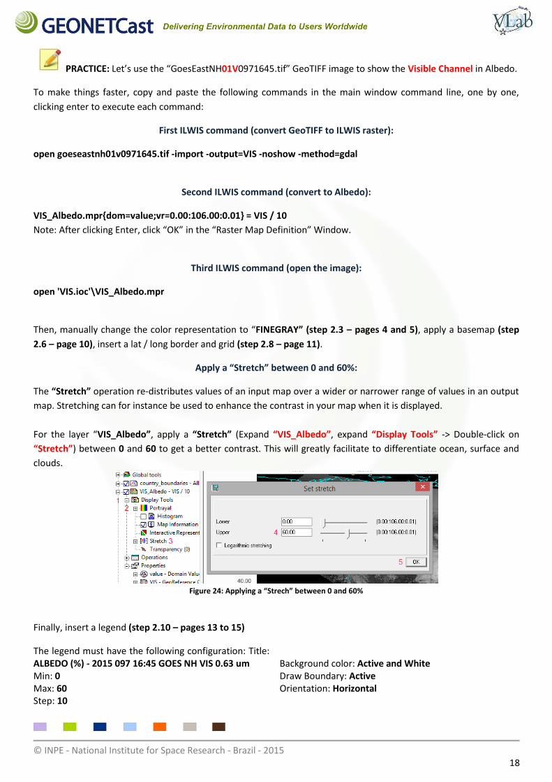
PRACTICE: Let’s use the “GoesEastNH04I30971645.tif” GeoTIFF image to show the Water Vapor Channel in
Celsius.
To make things faster, copy and paste the following commands in the main window command line, one by one,
clicking enter to execute each command:
First ILWIS command (convert GeoTIFF to ILWIS raster):
open goeseastnh04i30971645.tif -import -output=WV -noshow -method=gdal
Figure 23: Executing an operation using the command line
Second ILWIS command (convert to Celsius):
WV_Celsius.mpr{dom=value;vr=-273.17:-14.05:0.01} = (WV / 10) - 273.15
Note: After clicking Enter, click “OK” in the “Raster Map Definition” Window.
Third ILWIS command (open the image):
open 'WV.ioc'\WV_Celsius.mpr
Then, manually change the color representation to “WV_Celsius” (step 2.3 – pages 4 and 5), apply a basemap (step
2.6 – page 10), insert a lat / long border and grid (step 2.8 – page 11) and insert a legend (step 2.10 – pages 13 to
15)
The legend must have the following configuration:
Title: B. TEMPERATURE (C) - 2015 097 16:45 GOES NH WV 6.5um
Min: -80
Max: 0
Step: 20
Background color: Active and White
Draw Boundary: Active
Orientation: Horizontal
© INPE - National Institute for Space Research - Brazil - 2015 18
PRACTICE: Let’s use the “GoesEastNH01V0971645.tif” GeoTIFF image to show the Visible Channel in Albedo.
To make things faster, copy and paste the following commands in the main window command line, one by one,
clicking enter to execute each command:
First ILWIS command (convert GeoTIFF to ILWIS raster):
open goeseastnh01v0971645.tif -import -output=VIS -noshow -method=gdal
Second ILWIS command (convert to Albedo):
VIS_Albedo.mpr{dom=value;vr=0.00:106.00:0.01} = VIS / 10
Note: After clicking Enter, click “OK” in the “Raster Map Definition” Window.
Third ILWIS command (open the image):
open 'VIS.ioc'\VIS_Albedo.mpr
Then, manually change the color representation to “FINEGRAY” (step 2.3 – pages 4 and 5), apply a basemap (step
2.6 – page 10), insert a lat / long border and grid (step 2.8 – page 11).
Apply a “Stretch” between 0 and 60%:
The “Stretch” operation re-distributes values of an input map over a wider or narrower range of values in an output
map. Stretching can for instance be used to enhance the contrast in your map when it is displayed.
For the layer “VIS_Albedo”, apply a “Stretch” (Expand “VIS_Albedo”, expand “Display Tools” -> Double-click on
“Stretch”) between 0 and 60 to get a better contrast. This will greatly facilitate to differentiate ocean, surface and
clouds.
Figure 24: Applying a “Strech” between 0 and 60%
Finally, insert a legend (step 2.10 – pages 13 to 15)
The legend must have the following configuration: Title: ALBEDO (%) - 2015 097 16:45 GOES NH VIS 0.63 um Min: 0 Max: 60 Step: 10
Background color: Active and White Draw Boundary: Active Orientation: Horizontal
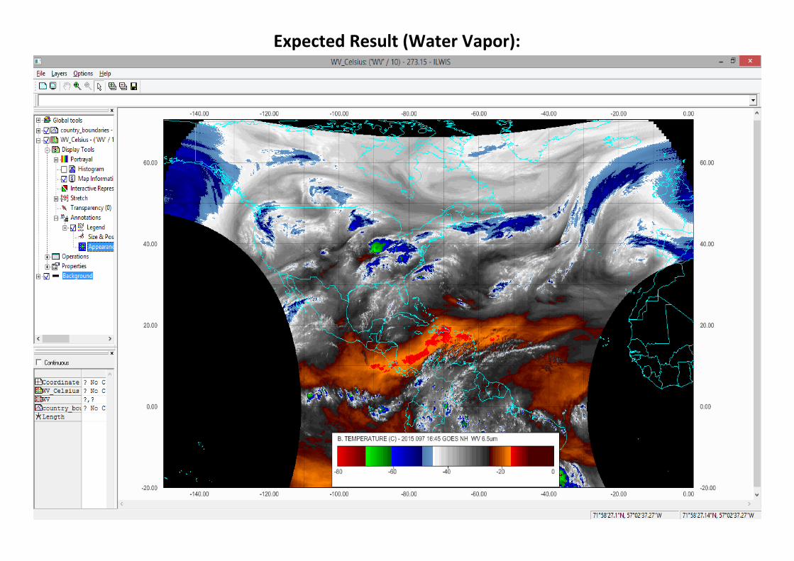
Expected Result (Water Vapor):
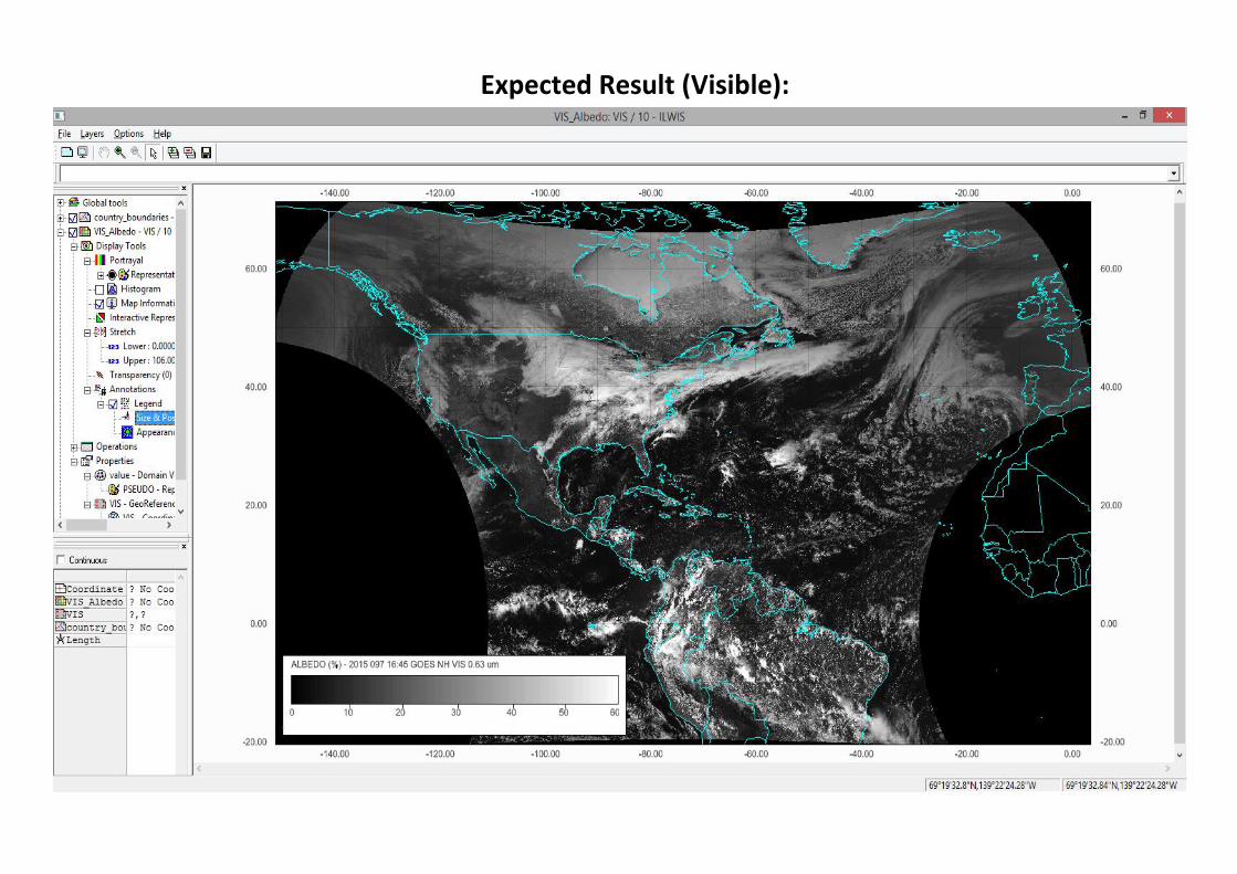
Expected Result (Visible):