Tunable Diode Laser (TDL) based Hydrogen Chloride gas (HCl) Continuous Emission Monitoring System (CEMS)

Development Challenges to Meet EPA’s Draft Performance Specification

Keith Crabbe Cemtek Environmental, Santa Ana, CA

Gervase Mckay

Unisearch Associates, Toronto, ON CAN Paul Tran Cemtek Environmental, Santa Ana, CA John T. Pisano and Thomas D. Durbin Department of Chemical and Environmental Engineering, Bourns College of Engineering, Center for Environmental Research and Technology (CE-CERT) University of California, Riverside, CA

ABSTRACT

New regulations and emissions limits are requiring the measurement and reporting of Hydrogen Chloride gas (HCl) levels. Both the Utility Boiler and Portland Cement Maximum Achievable Control Technology (MACT) rules for the first time require industry wide measurements for regulatory reporting requirements. Cemtek Environmental and Unisearch Associates have been involved in the HCl monitoring Performance Specification stakeholder’s group information exchange with the Environmental Protection Agency (EPA) for development of the new Draft Performance Specification for HCl CEMS. Cemtek has participated in a demonstration test at a North American cement manufacturing facility which investigated the performance of Tunable Diode Laser based HCl CEMS as outlined in the draft performance specification. This paper will present the demonstration field setup, the tests conducted including comparison with reference method, and obstacles and lessons learned in completing the tests along with additional laboratory trial results.

INTRODUCTION The United Sates Environmental Protection agency has put in place new rule regulating the emission of Hydrogen Chloride gas (HCl) from Stationary sources. These rules include the amendments to the NESHAP for Portland cement plants and to the NSPS for Portland cement plants and Coal fired Electric utility plants under the Mercury and Air Toxics Rule (MATS). These rules finalize standards that originated with Clean Air Act of 1990. At the time this study began the EPA regulations at 40CFR63, Subpart LLL which require installation, certification, operation and ongoing quality assurance of HCl CEMS to demonstrate continuous compliance with a 3 ppm HCl corrected to 7% O2, dry basis emission limit on a 30-day rolling average by not later than September 2013. Holcim Inc. developed, planned and executed a field evaluation project of four HCl CEMS at its St. Genevieve plant during the summer and fall of 2012. The general objectives of the study were to determine if contemporary HCl continuous emission monitoring systems (CEMS) have the capability, accuracy, precision and reliability. Cemtek Environmental using a Unisearch Associates HCl TDL analyzer was invited to participate in this evaluation. CEMTEK’s interest was to perform and practice some of the tests in the EPA draft performance specification 18. At the same time we were providing comments and feed back to the EPA team developing the PS as a stakeholder. The results of this effort are presented here along with some observations and issues in the conclusion of the report. (1)

EXPERIMENTAL

The study was conducted at the St. Genevieve plant under the direction of Glen Rosenhamer, Corporate Environmental Manager. Michelle Ferguson, Plant Environmental Manager, Aaron Dwyer (Electrical Superintendent), Rodney Miller (Instrumentation Specialist) provided extensive support for the project over many months. Jim Peeler, Emission Monitoring Inc. (EMI) provided consulting assistance during the entire project, participated in the field test, and prepared this report. Phil Kauppi, Prism Analytical Technologies, Inc. performed the FTIR testing for the stratification test, the Method 321 tests for the RATAs, and analyzed numerous compressed gas cylinders. (1) The Holcim St. Genevieve (GV) plant is a contemporary preheater precalciner kiln system which began operation during 2009. The kiln system has two inline raw mills and operating conditions include: (a) both raw mills operating, (b) one raw mill operating, and (c) no raw mills operating. These operating conditions affect the associated effluent HCl concentrations, the concentrations of other effluent components including NH3, as well as the effluent gas temperatures. HCl effluent concentrations varied over a range of 0-20 ppm, wet basis. Effluent gas temperatures also vary with operating condition and were expected to be approximately 205°F (two mills on), 255°F (one mill on) and 320°F (no mills operating). (1)

INSTRUMENTATION Tunable Diode Lasers (TDL’s) have special properties based upon small crystals (about 0.1 mm2) made of a mixture of elements such as gallium, arsenic, antimony and phosphorus. The proper selection and proportion of these elements the crystal can be made to emit at wavelengths where the target gas, which is HCl in this application, absorbs radiation of a particular energy. Changing either the temperature or current through the laser permits the wavelength to be tuned over the selected absorption feature of the target molecule. When an electric current is passed through these crystals they emit very pure laser light in the near-infrared spectral region. The temperature of the laser, which is stabilized with a thermoelectric cooler, will roughly establish the wavelength near the target gas’ absorption feature. The laser current is then simultaneously modulated in the kilohertz region so that phase sensitive detection techniques may be used to improve sensitivity. One advantage of the TDL technology is that the presence of the measured component in the gas stream can be used as a reference point for the laser itself. This function is called “line locking” and consists of the absorption peak of the HCl being used to keep the laser at the desired frequency. However, in the absence of the measurement component, during bypass or scheduled shutdowns, the laser can drift, and be outside calibration when the measurement component returns. To avoid drift, this TDL is supplied with a sealed internal reference cell, which contains a known amount of the gas to be measured. The use of the reference cells allows for not only line locking of the analyzer, but also the ability to continuously monitor the instrument’s calibration. We conducted some testes using this cell to report calibration drift test results in the results section of this study. The calculations which determine the actual gas concentration use Beer-Lambert Law.

I = Ioe-cl (1)

Where:

I = Intensity of light after absorption by target molecule Io = Intensity of light with no absorption by target molecule = Absorption cross section (species specific) c = Concentration (number density) of target molecule l = Path length Beer’s Law is based on the relative absorption of light at wavelengths which are not absorbed versus light which is absorbed by the molecule of interest. The intensities I and Io are determined by scanning the wavelength using the characteristic tunability of diode lasers, which allows the emission wavelength to be adjusted over a span of a few nanometers. This is sufficient to span certain absorption features in molecules such as ammonia, carbon monoxide, methane, and others. The only important variable is the fraction of light which is absorbed at the middle of the scan (return power, I) vs. the extreme ends of the scan (initial power, Io). The laser is scanned at a frequency of approximately 4 kHz, or every 250 micro seconds (s) so that variations in Io due to external factors (such as changing dust levels) will be very small. The error introduced by averaging Io over this very short interval is negligible. The most important consequence of this is that the absolute light levels reaching the detector are not important in determining

concentrations. It should be noted that this method actually responds to the total number of absorbing species present. The value is reported as a path averaged concentration, distributed along the entire measurement path.

A typical system configuration consists of the Analyzer unit in either stand alone or 19” rack mount configuration, which contains the TDL and associated electronics for signal transmittal and signal analysis. The Optical heads which contain the Launch and Receive components are mounted on the duct or stack and connected to the Analyzer via Fiber Optic/Coax cabling. This permits the analyzer to be placed in any suitable location, such as the CEM shelter or control room of the plant where it is not subjected to harsh environments and where it can be readily serviced as required. The optical signal is conveyed from the instrument to the measurement location by fiber optics and the return detected signal transported to the instrument by a separate coaxial cable. Thus, for example, continuous measurements can be made of the emissions in stacks and ducts which can be as much as 1500 feet (with a Photo Detector Amplifier or PDA) away from the instrument.

MEASUREMENT LOCATION If the measurement is being made for stack emissions monitoring or HCl CEMS, it is on the stack or at another location that would be considered representative of stack emissions. The EPA is referring to the cross stack as Integrated Path or IP-CEMS in the draft PS-18. The measurement sensitivity is dependent upon the measuring path length (Beer–Lambert law) and the opaqueness (particulate matter density) of the gas stream. The path length distance between the light source and the detector can vary depending upon the sample stream’s particulate concentration. Monitoring locations that have conditions such as a fully saturated or condensing stack or duct that has a similar effect as high dust loading, which would extinguish the laser light, should be avoided. Therefore when choosing the measurement location, these factors along with the turbulence and stratification issues that arise must be considered. The measurements are usually made in-situ across the stack or duct. Various configurations can be chosen to define the process interface by the choice of flange sizes, materials, purging modes and purging media in order to adapt the sensors for process engineering measurements. In some cases, the optical path can be inside a probe. However, this will limit the path length. Alignment of the optical heads are of significant importance, and therefore the sight tubes to which the optics are attached to, are required to be aligned to specific tolerance typically within 1 degree and must be maintained at relative high temperatures. The optical heads must have the capability to adjust for any small misalignment errors. Another component that must be taken into account is the “thermal growth” of the duct or stack and material aging. Several engineered solutions are available to counteract this issue. Two methods are employed for measurements across stacks or ducts: 1) single-pass where the laser radiation is transmitted across the stack to the detector on the other side, and 2) dual-pass where the laser radiation is transmitted across the stack to a reflector and then back to the detector on the same side as the transmitter. In typical installations, instrument air is used at each of the optical lenses to keep them clear of flue gas contaminants.

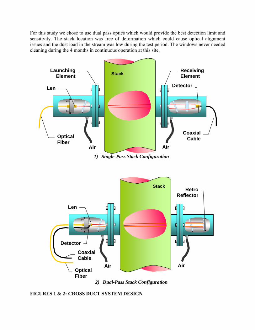
For this study we chose to use dual pass optics which would provide the best detection limit and sensitivity. The stack location was free of deformation which could cause optical alignment issues and the dust load in the stream was low during the test period. The windows never needed cleaning during the 4 months in continuous operation at this site.

1) Single-Pass Stack Configuration

2) Dual-Pass Stack Configuration

FIGURES 1 & 2: CROSS DUCT SYSTEM DESIGN

Optical Fiber

Len

Detector

Coaxial Cable

Stack

Air Air

RetroReflector

Optical Fiber

Len Detector

CoaxialCable

Stack

AirAir

LaunchingElement

Receiving Element

In special situations where long spool pieces or lagging is employed, especially in the prescience of negative pressure stacks or ducts, blowers are required to prevent the migration of HCl in the spool pieces. Such migration would cause a variable and inconsistent concentration of HCl in the laser path resulting in inconsistent and inaccurate measurements. Applying a positive pressure of ambient air to the spool pieces will assure that no stack gas HCl is migrating into the spool pieces. Particular attention must also be paid to the location of the measurement tools to limit the accumulation of particulate matter which can not only cause loss of signal due to light scattering but also can result in physical changes in the alignment of the laser light requiring realignment after cleaning. The blower system we used during this study kept the optics clean so instrument air was not needed. SENSITIVITY AND DETECTION LIMIT The sensitivity and minimum detection limit of an absorption device are path length dependent. The longer the path length, the higher the absorption and the lower the sensitivity and detection limit. Therefore, longer path lengths result in better detect ability of low concentrations. Dust loading in the effluent stream has the effect of blocking and scattering the laser radiation such that the detection limit will be compromised, leading to a much higher minimum detection value, due to lower power levels of the laser radiation reaching the detector. While particulate matter affects the detection limit, most systems can tolerate laser radiation power reductions of up to 90% without affecting the accuracy of the measurement. Nevertheless, there is a trade off in path length considerations between detect ability and reliability of the measurement. A single pass system with a PDA is recommended for high dust applications. Water vapor is also active in the near-IR spectral region; however the HCl line selected was far from waters influence. Typical sensitivity and detection limits on coal fired sources dependent on the above criteria would be ±1 ppmv with a detection limit of 0.2 part per million by volume (ppmv) respectively. CALIBRATION REQUIREMENTS Prior to initial usage, the instrument must be calibrated for HCl using a gas standard. After the initial calibration is performed, system validation is performed on a regular basis as defined by the governing body, in this case the USEPA. A flow-through gas cell permanently in the optical path that allows for introduction of cylinder gases to be injected to check the analyzer response as an additive or dynamic spike should be part of the analyzer. After use the cell is purged with dry air or nitrogen.

CALIBRATION FACTOR The TDL uses the Beer-Lambert Law to convert a quantity of absorption into a concentration as follows:

L

IIVTC L )ln( 0 (2)

Where:

is the line strength factor at STP I is the amount of measured light after passing through the gas medium

0I is the amount of initial light (i.e. transmitted light with no gas present that is to be

measured) L is the length of the absorption medium (Path length) V is the volume correction

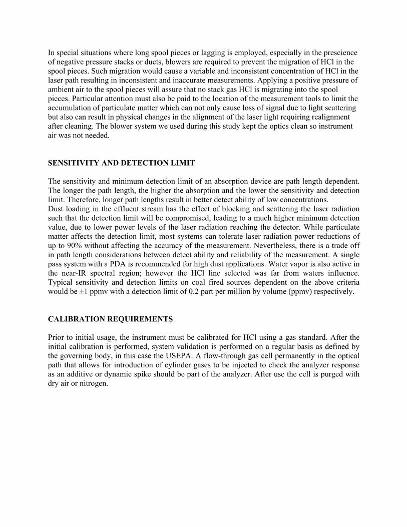
LT is the line strength correction (a function of gas temperature) When we do the initial calibration of the instruments we use a certified cylinder of gas, and re-arrange the equation to solve for . The test configuration shown in figure 3 has the double pass stack optics with a single blower at the stack. The analyzer is remotely located in a nearby CEMS shelter that is air conditioned and protected from the elements.

FIGURE 3: SYSTEM DESIGN

The power supply has an uninterruptable power supply (UPS) which provided power to the analyzer and programmable controller (PLC). The PLC is used to conduct the spike gas selection solenoid valves and sequences in the test configuration. The gases are conveyed to the flow-thru gas cell inside the analyzer with ¼ Teflon tubing. A laptop PC captures the data form the analyzer and provides a convenient interface with the analyzer. For this test we used it to connect to a wireless internet connection for remote support. In permanent installation the laptop is only used for troubleshooting and changing configuration parameters SPIKE GAS DETERMINATION To determine the spike gas injections for the appropriate values need to perform the tests we need to account for the path length. The cylinder values when using the IP-CEMS are larger than the fully extractive CEMS since the concentrations is divided by the path length. Below is the formula used to calculate the expected analyzer response to a known HCl concentration with a zero HCl background:

LSMT

T

PL

PLCC

roombottle

stack

stack

cellbottlespike

/

(3)

Where spikeC = Expected concentration of gas spike response in ppmv

bottleC = Concentration of gas cylinder in ppmv

cellPL = Path length of flow-thru gas cell in meters

stackPL = Path length of stack in meters

stackT = Temperature of stack in Kelvin

roombottleT / = Temperature of bottle/room in Kelvin

LSM = Line strength multiplier The cell length used in this analyzer was measured to be 0.158 m and the stack path length was 11.12 m. TESTS CONDUCTED ARE FROM THE DRAFT PS 18 FOR IP-CEMS This section describes the performance specification 18 tests that are required for IP-CEMS to performance to demonstrate initial certification and in some cases includes our interpretation. Then we report our findings in the discussion and results section for ht testes we attempted. (3)

Interference Test

Limit of Detection (LOD) Determination

Response Time Test

Calibration Error (CE) Test

Seven Day Calibration Drift Test

Stratification Test

Relative Accuracy Test or Dynamic Spiking Test

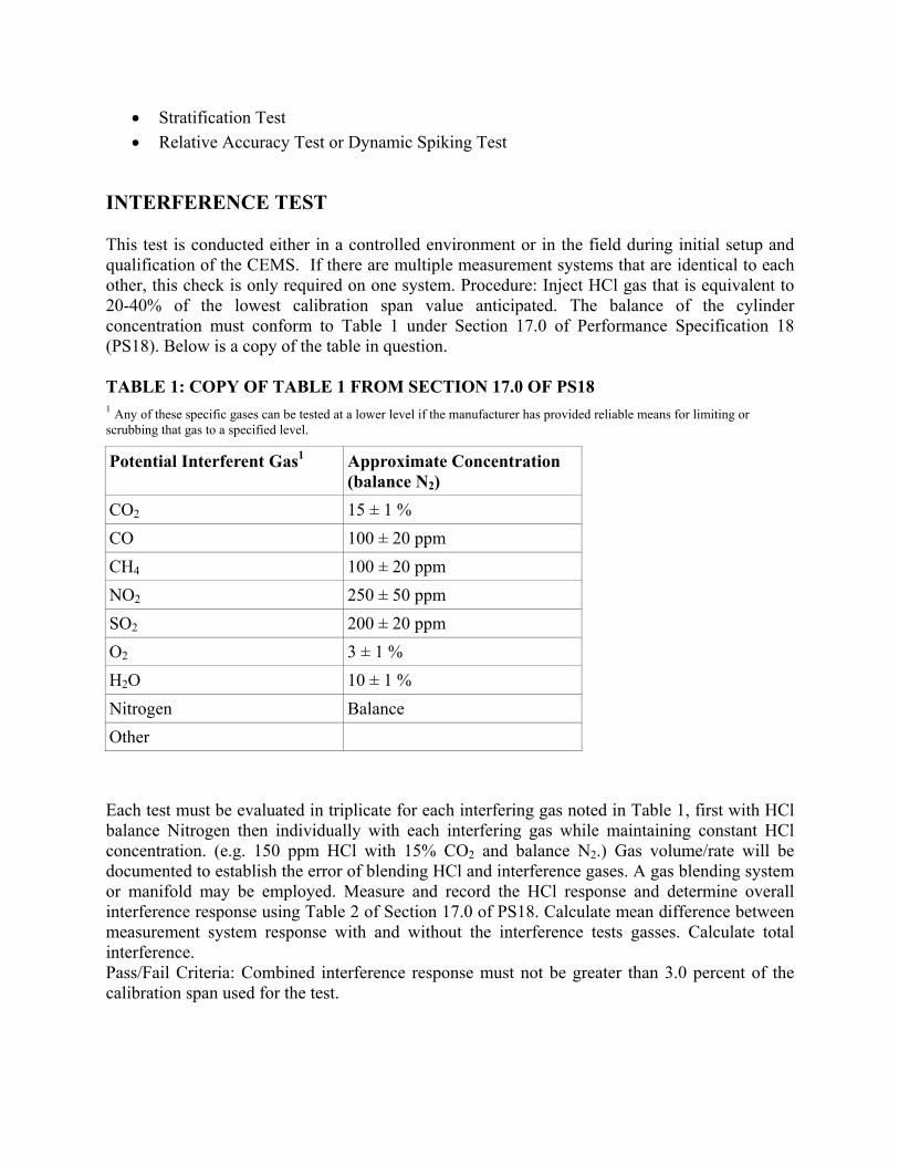
INTERFERENCE TEST This test is conducted either in a controlled environment or in the field during initial setup and qualification of the CEMS. If there are multiple measurement systems that are identical to each other, this check is only required on one system. Procedure: Inject HCl gas that is equivalent to 20-40% of the lowest calibration span value anticipated. The balance of the cylinder concentration must conform to Table 1 under Section 17.0 of Performance Specification 18 (PS18). Below is a copy of the table in question. TABLE 1: COPY OF TABLE 1 FROM SECTION 17.0 OF PS18 1 Any of these specific gases can be tested at a lower level if the manufacturer has provided reliable means for limiting or scrubbing that gas to a specified level.

Potential Interferent Gas1 Approximate Concentration (balance N2)

CO2 15 ± 1 %

CO 100 ± 20 ppm

CH4 100 ± 20 ppm

NO2 250 ± 50 ppm

SO2 200 ± 20 ppm

O2 3 ± 1 %

H2O 10 ± 1 %

Nitrogen Balance

Other

Each test must be evaluated in triplicate for each interfering gas noted in Table 1, first with HCl balance Nitrogen then individually with each interfering gas while maintaining constant HCl concentration. (e.g. 150 ppm HCl with 15% CO2 and balance N2.) Gas volume/rate will be documented to establish the error of blending HCl and interference gases. A gas blending system or manifold may be employed. Measure and record the HCl response and determine overall interference response using Table 2 of Section 17.0 of PS18. Calculate mean difference between measurement system response with and without the interference tests gasses. Calculate total interference. Pass/Fail Criteria: Combined interference response must not be greater than 3.0 percent of the calibration span used for the test.

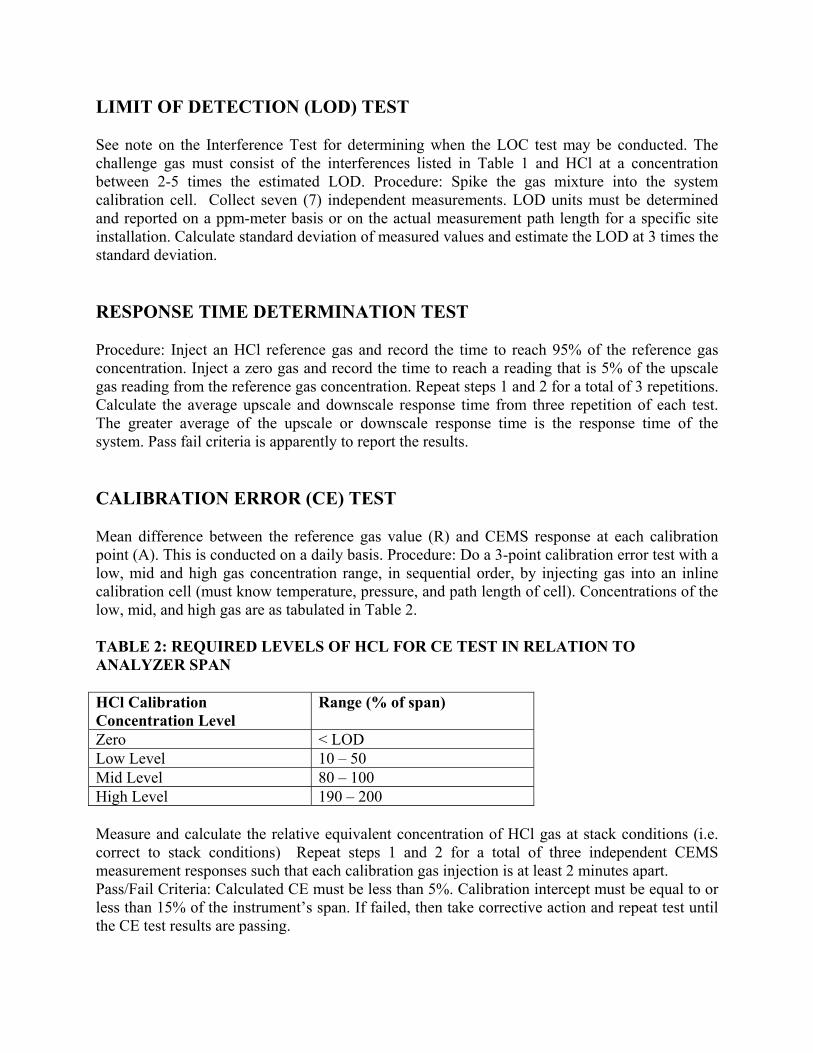
LIMIT OF DETECTION (LOD) TEST See note on the Interference Test for determining when the LOC test may be conducted. The challenge gas must consist of the interferences listed in Table 1 and HCl at a concentration between 2-5 times the estimated LOD. Procedure: Spike the gas mixture into the system calibration cell. Collect seven (7) independent measurements. LOD units must be determined and reported on a ppm-meter basis or on the actual measurement path length for a specific site installation. Calculate standard deviation of measured values and estimate the LOD at 3 times the standard deviation. RESPONSE TIME DETERMINATION TEST Procedure: Inject an HCl reference gas and record the time to reach 95% of the reference gas concentration. Inject a zero gas and record the time to reach a reading that is 5% of the upscale gas reading from the reference gas concentration. Repeat steps 1 and 2 for a total of 3 repetitions. Calculate the average upscale and downscale response time from three repetition of each test. The greater average of the upscale or downscale response time is the response time of the system. Pass fail criteria is apparently to report the results. CALIBRATION ERROR (CE) TEST Mean difference between the reference gas value (R) and CEMS response at each calibration point (A). This is conducted on a daily basis. Procedure: Do a 3-point calibration error test with a low, mid and high gas concentration range, in sequential order, by injecting gas into an inline calibration cell (must know temperature, pressure, and path length of cell). Concentrations of the low, mid, and high gas are as tabulated in Table 2. TABLE 2: REQUIRED LEVELS OF HCL FOR CE TEST IN RELATION TO ANALYZER SPAN HCl Calibration Concentration Level

Range (% of span)

Zero < LOD Low Level 10 – 50 Mid Level 80 – 100 High Level 190 – 200 Measure and calculate the relative equivalent concentration of HCl gas at stack conditions (i.e. correct to stack conditions) Repeat steps 1 and 2 for a total of three independent CEMS measurement responses such that each calibration gas injection is at least 2 minutes apart. Pass/Fail Criteria: Calculated CE must be less than 5%. Calibration intercept must be equal to or less than 15% of the instrument’s span. If failed, then take corrective action and repeat test until the CE test results are passing.

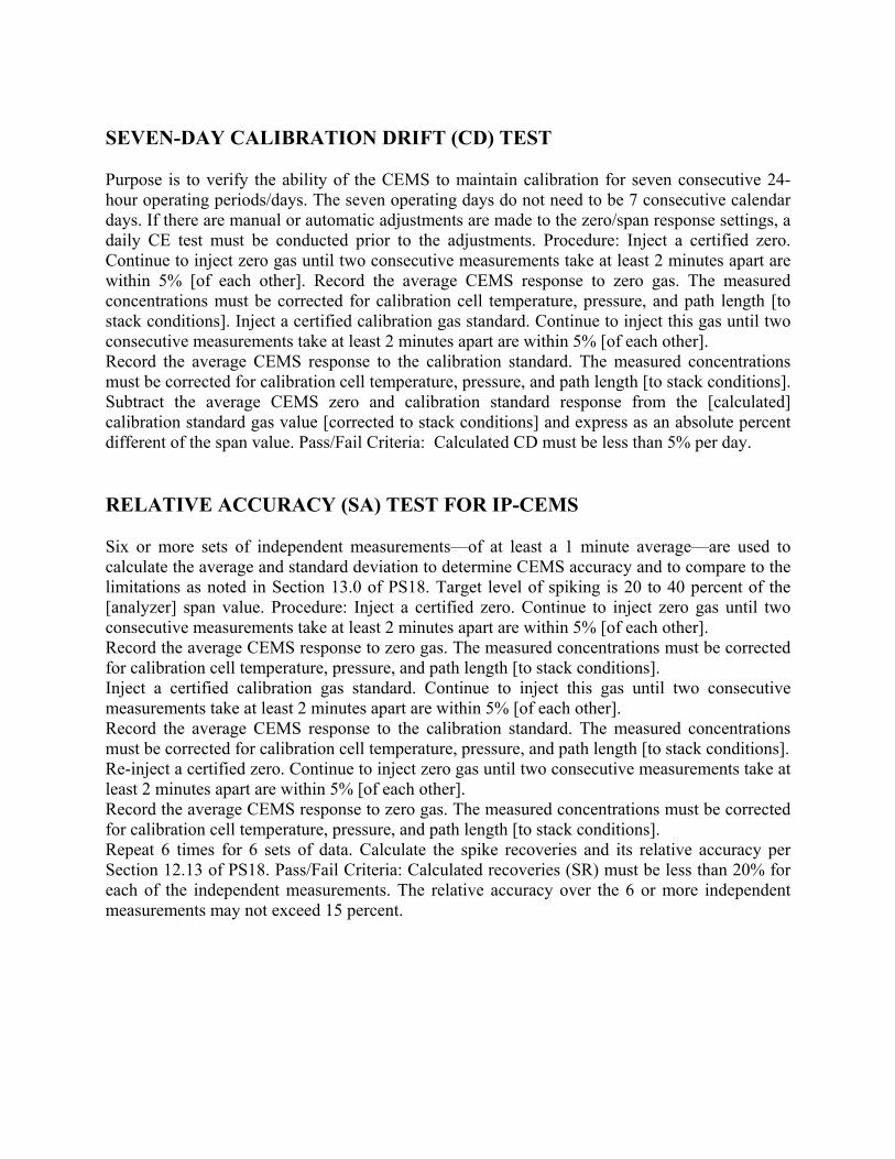
SEVEN-DAY CALIBRATION DRIFT (CD) TEST Purpose is to verify the ability of the CEMS to maintain calibration for seven consecutive 24-hour operating periods/days. The seven operating days do not need to be 7 consecutive calendar days. If there are manual or automatic adjustments are made to the zero/span response settings, a daily CE test must be conducted prior to the adjustments. Procedure: Inject a certified zero. Continue to inject zero gas until two consecutive measurements take at least 2 minutes apart are within 5% [of each other]. Record the average CEMS response to zero gas. The measured concentrations must be corrected for calibration cell temperature, pressure, and path length [to stack conditions]. Inject a certified calibration gas standard. Continue to inject this gas until two consecutive measurements take at least 2 minutes apart are within 5% [of each other]. Record the average CEMS response to the calibration standard. The measured concentrations must be corrected for calibration cell temperature, pressure, and path length [to stack conditions]. Subtract the average CEMS zero and calibration standard response from the [calculated] calibration standard gas value [corrected to stack conditions] and express as an absolute percent different of the span value. Pass/Fail Criteria: Calculated CD must be less than 5% per day. RELATIVE ACCURACY (SA) TEST FOR IP-CEMS Six or more sets of independent measurements—of at least a 1 minute average—are used to calculate the average and standard deviation to determine CEMS accuracy and to compare to the limitations as noted in Section 13.0 of PS18. Target level of spiking is 20 to 40 percent of the [analyzer] span value. Procedure: Inject a certified zero. Continue to inject zero gas until two consecutive measurements take at least 2 minutes apart are within 5% [of each other]. Record the average CEMS response to zero gas. The measured concentrations must be corrected for calibration cell temperature, pressure, and path length [to stack conditions]. Inject a certified calibration gas standard. Continue to inject this gas until two consecutive measurements take at least 2 minutes apart are within 5% [of each other]. Record the average CEMS response to the calibration standard. The measured concentrations must be corrected for calibration cell temperature, pressure, and path length [to stack conditions]. Re-inject a certified zero. Continue to inject zero gas until two consecutive measurements take at least 2 minutes apart are within 5% [of each other]. Record the average CEMS response to zero gas. The measured concentrations must be corrected for calibration cell temperature, pressure, and path length [to stack conditions]. Repeat 6 times for 6 sets of data. Calculate the spike recoveries and its relative accuracy per Section 12.13 of PS18. Pass/Fail Criteria: Calculated recoveries (SR) must be less than 20% for each of the independent measurements. The relative accuracy over the 6 or more independent measurements may not exceed 15 percent.

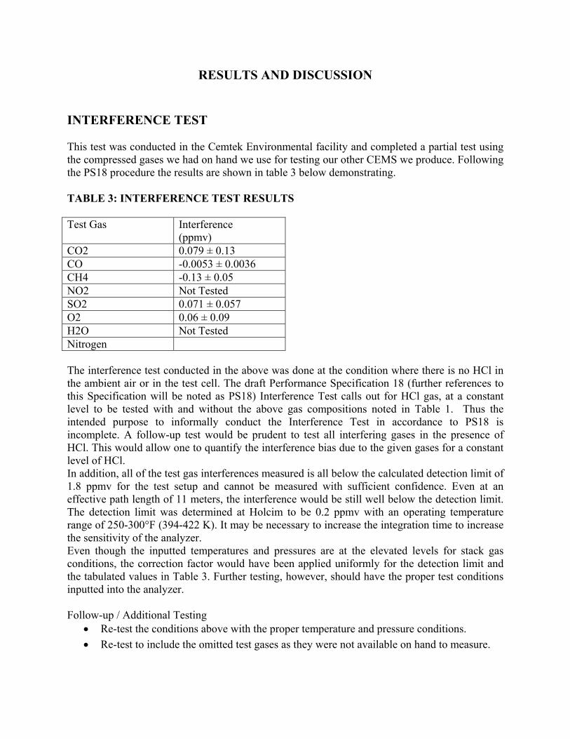
RESULTS AND DISCUSSION INTERFERENCE TEST This test was conducted in the Cemtek Environmental facility and completed a partial test using the compressed gases we had on hand we use for testing our other CEMS we produce. Following the PS18 procedure the results are shown in table 3 below demonstrating. TABLE 3: INTERFERENCE TEST RESULTS Test Gas Interference

(ppmv) CO2 0.079 ± 0.13 CO -0.0053 ± 0.0036 CH4 -0.13 ± 0.05 NO2 Not Tested SO2 0.071 ± 0.057 O2 0.06 ± 0.09 H2O Not Tested Nitrogen The interference test conducted in the above was done at the condition where there is no HCl in the ambient air or in the test cell. The draft Performance Specification 18 (further references to this Specification will be noted as PS18) Interference Test calls out for HCl gas, at a constant level to be tested with and without the above gas compositions noted in Table 1. Thus the intended purpose to informally conduct the Interference Test in accordance to PS18 is incomplete. A follow-up test would be prudent to test all interfering gases in the presence of HCl. This would allow one to quantify the interference bias due to the given gases for a constant level of HCl. In addition, all of the test gas interferences measured is all below the calculated detection limit of 1.8 ppmv for the test setup and cannot be measured with sufficient confidence. Even at an effective path length of 11 meters, the interference would be still well below the detection limit. The detection limit was determined at Holcim to be 0.2 ppmv with an operating temperature range of 250-300°F (394-422 K). It may be necessary to increase the integration time to increase the sensitivity of the analyzer. Even though the inputted temperatures and pressures are at the elevated levels for stack gas conditions, the correction factor would have been applied uniformly for the detection limit and the tabulated values in Table 3. Further testing, however, should have the proper test conditions inputted into the analyzer. Follow-up / Additional Testing

Re-test the conditions above with the proper temperature and pressure conditions.

Re-test to include the omitted test gases as they were not available on hand to measure.

Increase the integration time to 1 minute or more from 10 seconds to improve the detection limit. This will not be required if the path length is increased such that the detection limit is lowered sufficiently.

Have a method of automating the switching of the calibration gases via a manifold. Will speed up the data acquisition portion of the test.

LIMIT OF DETECTION (LOD) TEST This test was conducted in the field at the Holcim trial and the results. Successively decreasing spike gas concentrations were introduced to the in-line audit cell by means of diluting the 318 ppm audit gas with nitrogen using the EMI gas dilution manifold. The diluted spike concentration of 9.9 ppm is equivalent to an effluent HCl concentration of 0.165 ppm and was clearly distinguishable from the zero HCl concentration response of -0.005 ppm observed for the effluent after the spike was discontinued. Therefore the LOS for the TDL system as installed at St. Genevieve under real world conditions while actively monitoring cement kiln effluent is ≤ 0.16 ppm. Lower concentrations were spiked into the audit cell, however it was difficult to distinguish the presence of the response from the apparent zero value. (1)

RESPONSE TIME TEST Response Time Test Results were taken from the data collected performing calibration error tests using a bottle of HCl and Nitrogen supplied by Holcim and conducted after the completion of the Trial period. The results are show below. The optical setup was set up to have an effective path length of 11.12 meters. The temperature and pressure was dynamically inputted from the customer DCS. Integration time was left at 10 seconds. Calibration gas was introduced via a solenoid manifold assembly controlled by a PLC. The cylinder concentration employed was a 318.5 ppmv bottle. The average effective analyzer response is roughly 5 ppmv depending on the temperature conditions at the time of test. Procedure Gases were injected into the flow-through gas cell via solenoids. The sequence is automated by a PLC and is as follows.

1. 15 minute (900 seconds) delay after internal zero/audit check 2. Flow N2 gas for 120 seconds. Purge sequence 3. Flow HCl gas for 300 seconds 4. Flow N2 gas for 240 seconds. Purge/Zero sequence

The analyzer records the response in real-time as a flat text file. The data will be then pulled and analyzed accordingly. Results Tables 2 and 3 tabulate the raw data for the rise and fall of the HCl analyzer response average for each test run. Averages of the background data where no HCl was present were taken before and after to determine the background levels. The Analyzer Reponses takes this into account by

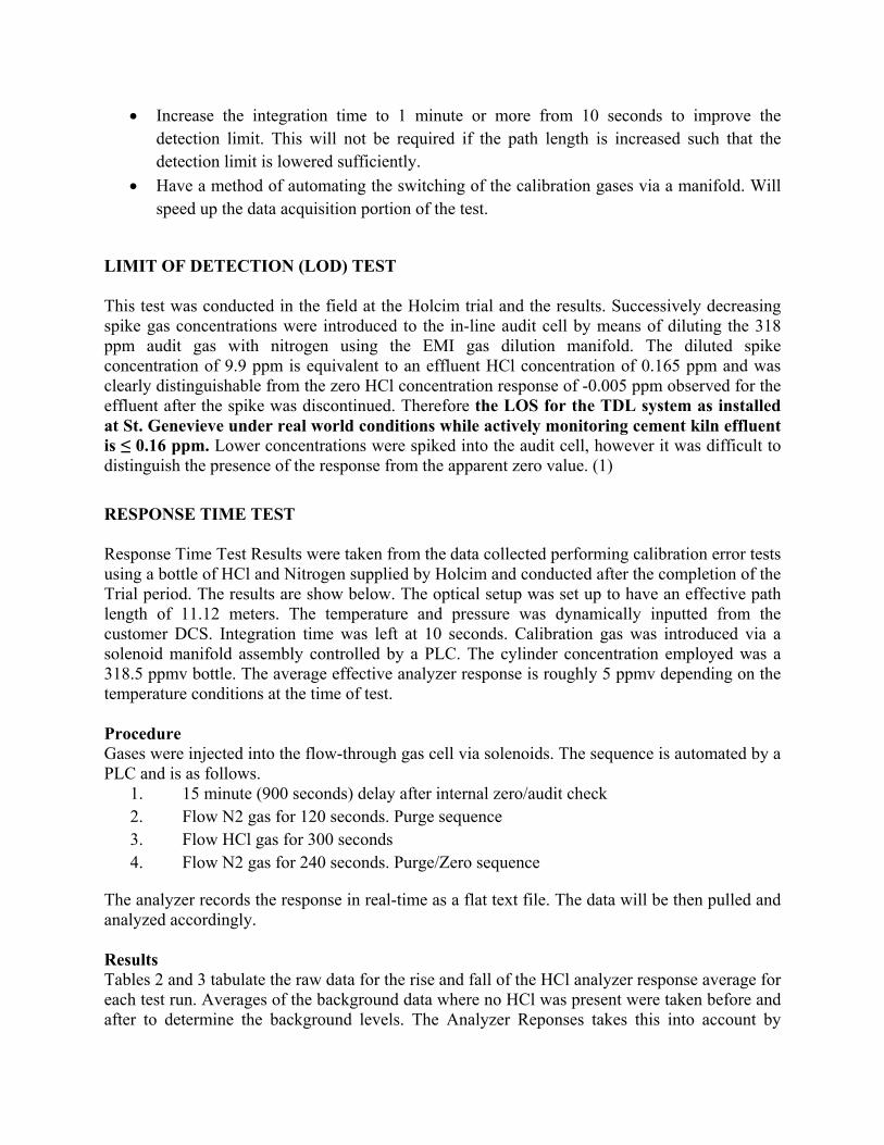
subtracting the background levels. Also included is the average temperature and expected analyzer response. Additionally, a non-linear total least squares fit has been applied to the data to determine the experimental time-constant k, which is noted below as Equation [1]. This was done via the Solver add-in in Excel. From the fitted time-constant, the time to reach 95% of the analyzer response was determined. This can be seen in Table 3 and graphically in Figures 4.

FIGURE 4: RESPONSE TIME TEST RESULTS Rise and Fall time graphs for Tests 1, 2, and 3. Shows the best fit to the data as solved

‐20

30

80

0 50 100

% Response

Time (s)

Test #1, Rise Time

y

Fit

‐20

0

20

40

60

80

100

120

0 50 100% Response

Time (s)

Test #1, Fall Time

y

Fit

‐20

0

20

40

60

80

100

120

0 50 100

% Response

Time (s)

Test #2, Rise Time

y

Fit

‐20

0

20

40

60

80

100

120

0 50 100

% Response

Time (s)

Test #2, Fall Time

y

Fit

0

20

40

60

80

100

120

0 50 100

% Response

Time (s)

Test #3, Rise Time

y

Fit

‐50

0

50

100

150

0 50 100

% Response

Time (s)

Test #3, Fall TIme

y

Fit

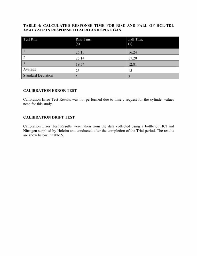
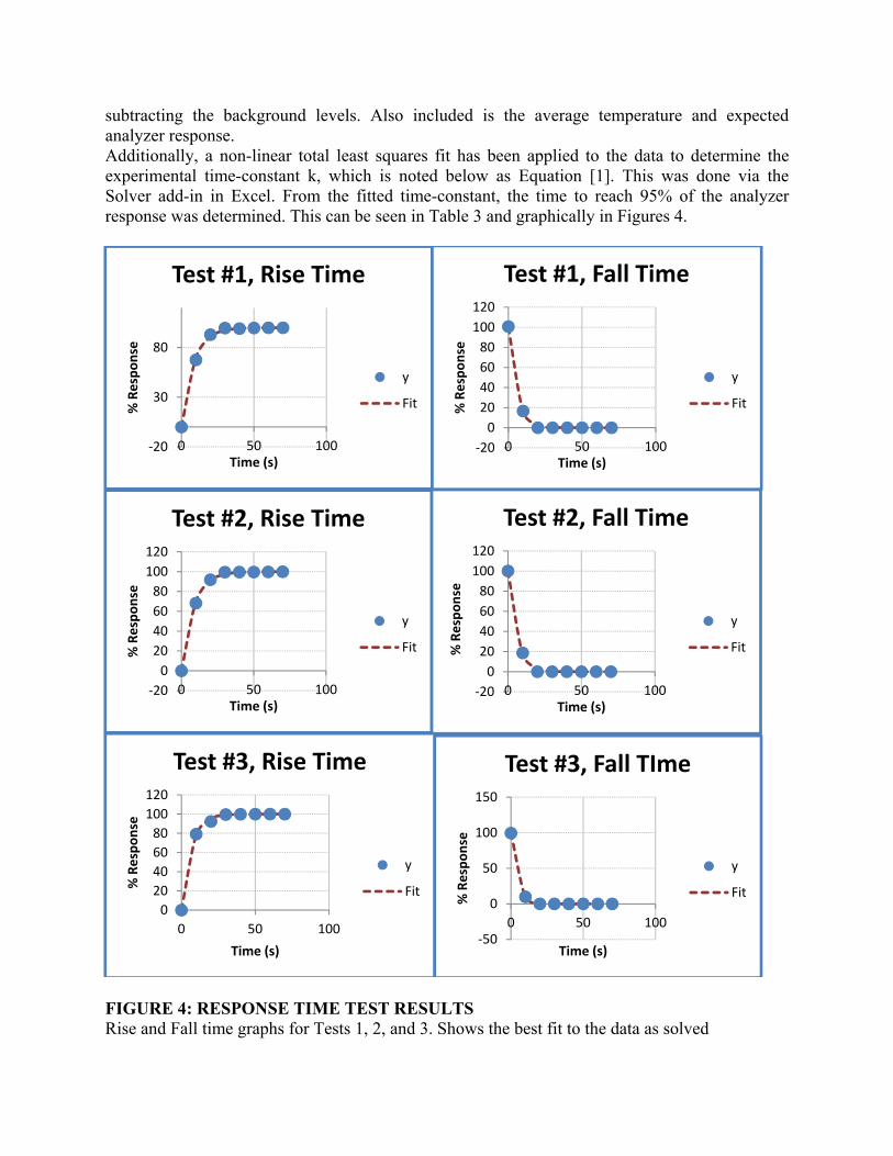
TABLE 4: CALCULATED RESPONSE TIME FOR RISE AND FALL OF HCL-TDL ANALYZER IN RESPONSE TO ZERO AND SPIKE GAS. Test Run Rise Time

(s) Fall Time (s)

1 25.10 16.24 2 25.14 17.20 3 19.74 12.81 Average 23 15 Standard Deviation 3 2 CALIBRATION ERROR TEST Calibration Error Test Results was not performed due to timely request for the cylinder values need for this study. CALIBRATION DRIFT TEST Calibration Error Test Results were taken from the data collected using a bottle of HCl and Nitrogen supplied by Holcim and conducted after the completion of the Trial period. The results are show below in table 5.

TABLE 5: CALIBRATION DRIFT TEST RESULTS

Daily Spiking Summary

Day Date #

Of readings

Pre-Spike Bkg

Average (ppm)

Post-Spike Bkg

Average (ppm)

HCl Baseline

(ppm)

Average AnalyzerResponse

(ppm)

Average Analyzer

Spike Reponse (ppm)

Tavg (K)

Expected Response

at Tavg (ppm)

SRavg (%)

SAavg (%)

Cal. Drift

0.0 10/16 13 0.00062 -0.00064 -0.00001 5.322 5.322 357.22 5.195 102.45% 3.44% 0.42%

0.1 10/16 13 -0.00032 -0.00040 -0.00036 4.959 4.959 359.12 5.215 95.08% 3.18% 0.85%

0.2 10/16 13 0.00053 0.00000 0.00027 5.455 5.455 386.72 5.522 98.79% 3.30% 0.22%

0.3 10/16 13 0.00286 0.00002 0.00144 5.847 5.846 383.50 5.486 106.57% 3.57% 1.20%

1.0 10/17 13 5.29874 5.60349 5.45112 11.888 6.437 442.42 6.170 104.31% 3.63% 0.89%

2.0 10/18 13 -0.00017 -0.00051 -0.00034 5.585 5.585 372.74 5.366 104.09% 3.48% 0.73%

3.0 10/19 13 -0.00018 -0.00023 -0.00021 5.640 5.640 376.29 5.405 104.35% 3.49% 0.78%

4.0 10/20 13 -0.00092 -0.00118 -0.00105 5.596 5.597 376.75 5.410 103.46% 3.46% 0.62%

5.0 10/21 13 -0.01857 -0.00504 -0.01180 5.277 5.289 362.12 5.248 100.77% 3.37% 0.14%

6.0 10/22 13 0.56555 0.35426 0.45991 7.136 6.676 419.30 5.896 113.24% 3.79% 2.60%

7.0 10/23 13 0.00342 0.00412 0.00377 5.787 5.783 373.52 5.374 107.61% 3.60% 1.36%

8.0 10/24 13 0.00009 0.00126 0.00068 5.778 5.778 378.99 5.435 106.30% 3.56% 1.14%

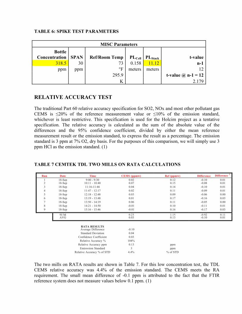
TABLE 6: SPIKE TEST PARAMETERS

RELATIVE ACCURACY TEST The traditional Part 60 relative accuracy specification for SO2, NOx and most other pollutant gas CEMS is ≤20% of the reference measurement value or ≤10% of the emission standard, whichever is least restrictive. This specification is used for the Holcim project as a tentative specification. The relative accuracy is calculated as the sum of the absolute value of the differences and the 95% confidence coefficient, divided by either the mean reference measurement result or the emission standard, to express the result as a percentage. The emission standard is 3 ppm at 7% O2, dry basis. For the purposes of this comparison, we will simply use 3 ppm HCl as the emission standard. (1)

TABLE 7 CEMTEK TDL TWO MILLS ON RATA CALCULATIONS

Run Date Time CEMS (ppmw) Ref (ppmw) Difference Difference 2

1 18-Sep 9:00 - 9:30 0.02 0.12 -0.10 0.012 18-Sep 10:11 - 10:40 0.07 0.15 -0.08 0.01 3 18-Sep 11:16-11:46 0.04 0.14 -0.10 0.01 4 18-Sep 11:47 - 12:17 0.02 0.11 -0.09 0.01 5 18-Sep 12:18 - 12:48 0.03 0.09 -0.06 0.00 6 18-Sep 13:19 - 13:48 0.01 0.17 -0.16 0.03 7 18-Sep 13:50 - 14:19 0.06 0.11 -0.05 0.00 8 18-Sep 14:21 - 14:50 -0.01 0.10 -0.11 0.01 9 18-Sep 15:16 - 15:46 -0.01 0.16 -0.17 0.03

SUM 0.23 1.15 -0.92 0.11

AVG 0.03 0.13 -0.10 0.01

RATA RESULTS

Average Difference -0.10 Standard Deviation 0.04

Confidence Coefficient 0.03 Relative Accuracy % 104%

Relative Accuracy ppm 0.13 ppm Emiswsion Standard 3 ppm

Relative Accuracy % of STD 4.4% % of STD  The two mills on RATA results are shown in Table 7. For this low concentration test, the TDL CEMS relative accuracy was 4.4% of the emission standard. The CEMS meets the RA requirement. The small mean difference of -0.1 ppm is attributed to the fact that the FTIR reference system does not measure values below 0.1 ppm. (1)

MISC Parameters

Bottle Concentration SPAN Ref/Room Temp PLCell PLStack t-value

318.5 30 73 0.158 11.12 n-1ppm ppm °F meters meters 12

295.9 t-value @ n-1 = 12K 2.179

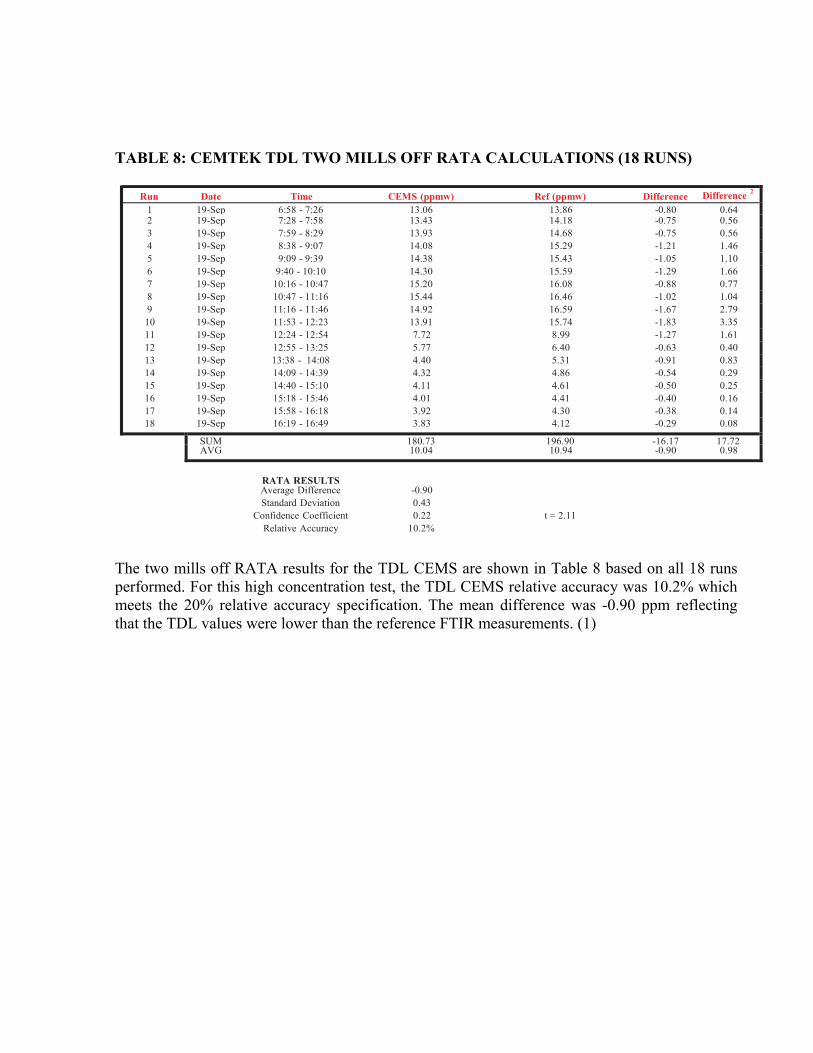
TABLE 8: CEMTEK TDL TWO MILLS OFF RATA CALCULATIONS (18 RUNS)

Run Date Time CEMS (ppmw) Ref (ppmw) Difference Difference 2

1 19-Sep 6:58 - 7:26 13.06 13.86 -0.80 0.642 19-Sep 7:28 - 7:58 13.43 14.18 -0.75 0.56 3 19-Sep 7:59 - 8:29 13.93 14.68 -0.75 0.56 4 19-Sep 8:38 - 9:07 14.08 15.29 -1.21 1.46 5 19-Sep 9:09 - 9:39 14.38 15.43 -1.05 1.10 6 19-Sep 9:40 - 10:10 14.30 15.59 -1.29 1.66 7 19-Sep 10:16 - 10:47 15.20 16.08 -0.88 0.77 8 19-Sep 10:47 - 11:16 15.44 16.46 -1.02 1.04 9 19-Sep 11:16 - 11:46 14.92 16.59 -1.67 2.79 10 19-Sep 11:53 - 12:23 13.91 15.74 -1.83 3.35 11 19-Sep 12:24 - 12:54 7.72 8.99 -1.27 1.61 12 19-Sep 12:55 - 13:25 5.77 6.40 -0.63 0.40 13 19-Sep 13:38 - 14:08 4.40 5.31 -0.91 0.83 14 19-Sep 14:09 - 14:39 4.32 4.86 -0.54 0.29 15 19-Sep 14:40 - 15:10 4.11 4.61 -0.50 0.25 16 19-Sep 15:18 - 15:46 4.01 4.41 -0.40 0.16 17 19-Sep 15:58 - 16:18 3.92 4.30 -0.38 0.14 18 19-Sep 16:19 - 16:49 3.83 4.12 -0.29 0.08

SUM 180.73 196.90 -16.17 17.72

AVG 10.04 10.94 -0.90 0.98

RATA RESULTS

Average Difference -0.90 Standard Deviation 0.43

Confidence Coefficient 0.22 t = 2.11 Relative Accuracy 10.2%

The two mills off RATA results for the TDL CEMS are shown in Table 8 based on all 18 runs performed. For this high concentration test, the TDL CEMS relative accuracy was 10.2% which meets the 20% relative accuracy specification. The mean difference was -0.90 ppm reflecting that the TDL values were lower than the reference FTIR measurements. (1)

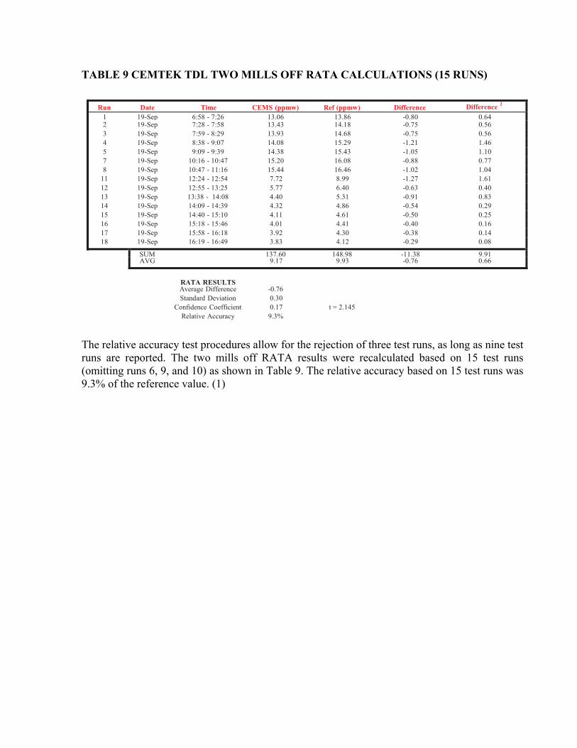
TABLE 9 CEMTEK TDL TWO MILLS OFF RATA CALCULATIONS (15 RUNS)

Run Date Time CEMS (ppmw) Ref (ppmw) Difference Difference 2

1 19-Sep 6:58 - 7:26 13.06 13.86 -0.80 0.642 19-Sep 7:28 - 7:58 13.43 14.18 -0.75 0.56 3 19-Sep 7:59 - 8:29 13.93 14.68 -0.75 0.56 4 19-Sep 8:38 - 9:07 14.08 15.29 -1.21 1.46 5 19-Sep 9:09 - 9:39 14.38 15.43 -1.05 1.10 7 19-Sep 10:16 - 10:47 15.20 16.08 -0.88 0.77 8 19-Sep 10:47 - 11:16 15.44 16.46 -1.02 1.04

11 19-Sep 12:24 - 12:54 7.72 8.99 -1.27 1.61 12 19-Sep 12:55 - 13:25 5.77 6.40 -0.63 0.40 13 19-Sep 13:38 - 14:08 4.40 5.31 -0.91 0.83 14 19-Sep 14:09 - 14:39 4.32 4.86 -0.54 0.29 15 19-Sep 14:40 - 15:10 4.11 4.61 -0.50 0.25 16 19-Sep 15:18 - 15:46 4.01 4.41 -0.40 0.16 17 19-Sep 15:58 - 16:18 3.92 4.30 -0.38 0.14 18 19-Sep 16:19 - 16:49 3.83 4.12 -0.29 0.08

SUM 137.60 148.98 -11.38 9.91

AVG 9.17 9.93 -0.76 0.66

RATA RESULTS

Average Difference -0.76 Standard Deviation 0.30

Confidence Coefficient 0.17 t = 2.145 Relative Accuracy 9.3%

The relative accuracy test procedures allow for the rejection of three test runs, as long as nine test runs are reported. The two mills off RATA results were recalculated based on 15 test runs (omitting runs 6, 9, and 10) as shown in Table 9. The relative accuracy based on 15 test runs was 9.3% of the reference value. (1)

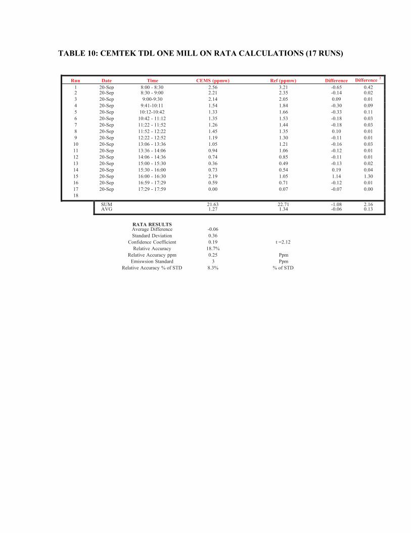
TABLE 10: CEMTEK TDL ONE MILL ON RATA CALCULATIONS (17 RUNS)

Run Date Time CEMS (ppmw) Ref (ppmw) Difference Difference 2

1 20-Sep 8:00 - 8:30 2.56 3.21 -0.65 0.422 20-Sep 8:30 - 9:00 2.21 2.35 -0.14 0.02 3 20-Sep 9:00-9:30 2.14 2.05 0.09 0.01 4 20-Sep 9:41-10:11 1.54 1.84 -0.30 0.09 5 20-Sep 10:12-10:42 1.33 1.66 -0.33 0.11 6 20-Sep 10:42 - 11:12 1.35 1.53 -0.18 0.03 7 20-Sep 11:22 - 11:52 1.26 1.44 -0.18 0.03 8 20-Sep 11:52 - 12:22 1.45 1.35 0.10 0.01 9 20-Sep 12:22 - 12:52 1.19 1.30 -0.11 0.01 10 20-Sep 13:06 - 13:36 1.05 1.21 -0.16 0.03 11 20-Sep 13:36 - 14:06 0.94 1.06 -0.12 0.01 12 20-Sep 14:06 - 14:36 0.74 0.85 -0.11 0.01 13 20-Sep 15:00 - 15:30 0.36 0.49 -0.13 0.02 14 20-Sep 15:30 - 16:00 0.73 0.54 0.19 0.04 15 20-Sep 16:00 - 16:30 2.19 1.05 1.14 1.30 16 20-Sep 16:59 - 17:29 0.59 0.71 -0.12 0.01 17 20-Sep 17:29 - 17:59 0.00 0.07 -0.07 0.00 18

SUM 21.63 22.71 -1.08 2.16

AVG 1.27 1.34 -0.06 0.13

RATA RESULTS

Average Difference -0.06 Standard Deviation 0.36

Confidence Coefficient 0.19 t =2.12 Relative Accuracy 18.7%

Relative Accuracy ppm 0.25 Ppm Emiswsion Standard 3 Ppm

Relative Accuracy % of STD 8.3% % of STD

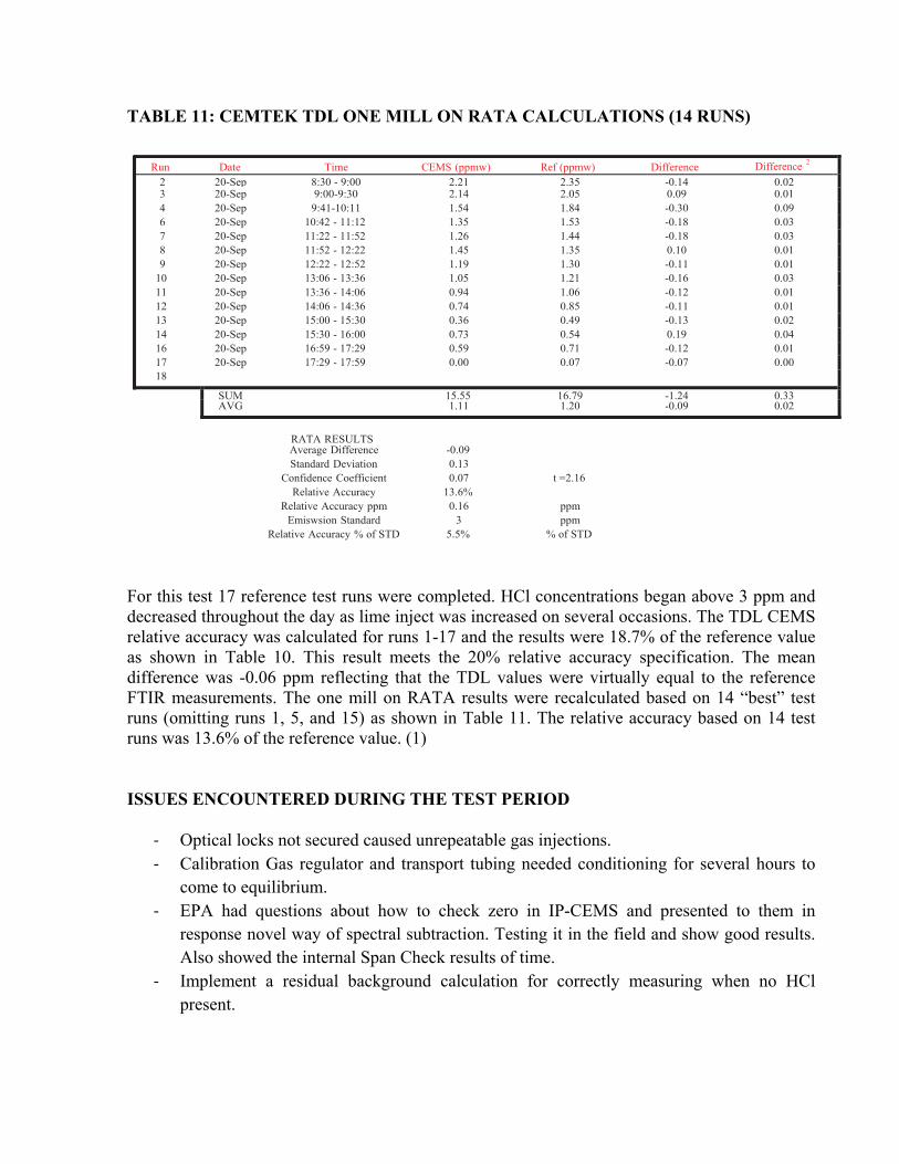
TABLE 11: CEMTEK TDL ONE MILL ON RATA CALCULATIONS (14 RUNS)

Run Date Time CEMS (ppmw) Ref (ppmw) Difference Difference 2

2 20-Sep 8:30 - 9:00 2.21 2.35 -0.14 0.023 20-Sep 9:00-9:30 2.14 2.05 0.09 0.01 4 20-Sep 9:41-10:11 1.54 1.84 -0.30 0.09 6 20-Sep 10:42 - 11:12 1.35 1.53 -0.18 0.03 7 20-Sep 11:22 - 11:52 1.26 1.44 -0.18 0.03 8 20-Sep 11:52 - 12:22 1.45 1.35 0.10 0.01 9 20-Sep 12:22 - 12:52 1.19 1.30 -0.11 0.01

10 20-Sep 13:06 - 13:36 1.05 1.21 -0.16 0.03 11 20-Sep 13:36 - 14:06 0.94 1.06 -0.12 0.01 12 20-Sep 14:06 - 14:36 0.74 0.85 -0.11 0.01 13 20-Sep 15:00 - 15:30 0.36 0.49 -0.13 0.02 14 20-Sep 15:30 - 16:00 0.73 0.54 0.19 0.04 16 20-Sep 16:59 - 17:29 0.59 0.71 -0.12 0.01 17 20-Sep 17:29 - 17:59 0.00 0.07 -0.07 0.00 18

SUM 15.55 16.79 -1.24 0.33

AVG 1.11 1.20 -0.09 0.02

RATA RESULTS

Average Difference -0.09 Standard Deviation 0.13

Confidence Coefficient 0.07 t =2.16 Relative Accuracy 13.6%

Relative Accuracy ppm 0.16 ppm Emiswsion Standard 3 ppm

Relative Accuracy % of STD 5.5% % of STD

For this test 17 reference test runs were completed. HCl concentrations began above 3 ppm and decreased throughout the day as lime inject was increased on several occasions. The TDL CEMS relative accuracy was calculated for runs 1-17 and the results were 18.7% of the reference value as shown in Table 10. This result meets the 20% relative accuracy specification. The mean difference was -0.06 ppm reflecting that the TDL values were virtually equal to the reference FTIR measurements. The one mill on RATA results were recalculated based on 14 “best” test runs (omitting runs 1, 5, and 15) as shown in Table 11. The relative accuracy based on 14 test runs was 13.6% of the reference value. (1) ISSUES ENCOUNTERED DURING THE TEST PERIOD

‐ Optical locks not secured caused unrepeatable gas injections. ‐ Calibration Gas regulator and transport tubing needed conditioning for several hours to

come to equilibrium. ‐ EPA had questions about how to check zero in IP-CEMS and presented to them in

response novel way of spectral subtraction. Testing it in the field and show good results. Also showed the internal Span Check results of time.

‐ Implement a residual background calculation for correctly measuring when no HCl present.

‐ Implementation of dynamic temperature inputs to analyzer. This employed was to account for the potentially wide swings in temperature at site. The expected error in the measurements would be in the range of 6 to 7% if a fixed temperature of 126.6°C was employed—thus a fixed calibration factor.

‐ Automated daily injections to the Cal Error test near the end of the trial period with very good results.

‐ Found better results by turning off low correlation R-value <0.7 correction. ‐ Difference found between the factory calibration factor as compared to specialty gas

cylinders of HCl. The Cal factor was set by an external audit module that was over 5 years old.

‐ Measurement by TDL is wet basis and compliance limit is 3 ppmvd at 7% O2 on a 30 –day rolling average.

CONCLUSIONS

The results obtained for the tests conducted for this study provide some of the first data from HCl CEMS while following the test procedures in Draft PS 18. The EPA has received this data to further their PS development. The interference test was partially completed and the results showed that for the interfering gases tested the TDL would pass the test for those gases. The responses were all below the LOD. This test will need to be performed for the complete list of gases and concentration ranges added to a base HCl concentration as the test calls out in future studies. An interference test was conducted by the University of California, Riverside with similar results. (3)

The limit of detection test showed that he TDL is a sensitive measurement technique and the result of this test exceeded the expectation of the manufacturer. The lab LOD was expected to be 0.2 ppmv and the measured LOD installed was better than that measuring 0.16 ppmv. Further installation test need to done to demonstrate repeat performance. (3)

The response time test used the spike test data and showed the response to the spike gas and zero gas was less than 30 seconds. Normal CEMS response time limits are 15 minutes maximum so this a very rapid repose time and can be useful for process control at this speed of analysis.

The calibration error test was not conducted during this study and will be conducted at another installation. We did prepare in time to select the gases needed before demobilizing form the field

The seven day drift results showed that using the internal Cal cell as well as the gas flow though demonstrated the stability and repeatability needed to pass this test. All testes were 2.6% and less.

The stratification test was not conducted during this study.

The relative accuracy test was evaluated as a 40CFRPart 60 CEMS would be evaluated. The TDL passed all the test conditions presented. Several conditions to generate low and high levels of HCl stack gas and all were within passing tolerances.

During the study period we also learned a number of things to make the analyzer perform better. Some were in the form of signal processing analysis. Some improvements is startup and commissioning procedure checklist were made. Over all the TDL was very simple to startup and maintain with very little attention need to obtain excellent results. ACKNOWLEDGEMENT Holcim Inc. and the staff at St. Genevieve plant. REFERENCES 1. Peeler. Jim - Emission Monitoring Inc., Rosenhamer, Glen - Holcim Inc., Field Evaluation of

HCl CEMS at Holcim St. Genevieve Plant, December 19, 2012

2. USEPA, Draft Version 9-19-2012, Draft Performance Specification 18, Performance Specifications and Test Procedures for HCl Continuous Emission Monitoring Systems in Stationary Sources

3. Dene, Chuck – EPRI, Continuous Emission Monitor For Hydrochloric Acid, Tunable Diode Laser Test Report, Unisearch LasIR S Series, 1022083, Final Report, December 2011 EPRI, Palo Alto, CA: 2011 1022083).