Transmission Cost Allocation Using the Distribution Factors Method

Stefan Kilyeni, Oana Pop, Titus Slavici, Cristian Craciun, Petru Andea, Dumitru Mnerie

"Politehnica" University of Timisoara Bd. Vasile Parvan, No. 1, 300223, Timisoara, Romania

stefan.kilyeni@et.upt.ro

oana.pop@et.upt.ro

Abstract— One of the key problems of energy transmission

system in an independent environment refers to necessity to establish a cost for system services on nondiscriminatory bases. The prices must to be simple and transparent. A properly established cost provides economical signals for short-term and long-term recovery current expenses and for a fair cost allocation for participants. This paper presents allocation of transmission costs to consumers and to generator using the distribution factors method. A detailed comparison between regime with active losses and the regime without active losses are presented. A case study based on a 12-node system is provided.

I. INTRODUCTION

The transmission cost [1], [2] is the most complicated issues in power system restructuring, because of physical laws, which governs the transmission network power flow. Since generators and consumers are connected to the transmission network, a participant’s action has consequences to other participants too, making difficultly the investigation of components price, which cost one to each participant [3], [4].

Transmission active loss allocation is the process of assigning to each individual generation and load the responsibility of paying for a part of the system transmission active losses. [5] Transmission active loss allocation is not an easy task. Loss allocation between the generator and the load has to be agreed upon as there is no physical measurement or mathematical method that determines the loss shares in a unique manner. [6] In a real system, matters get more complicated because of nonlinear function of the line power flow, and hence cannot be separated between partial flows through the same line in a unique convincing way.

In this paper an analysis of the allocation method using distribution factors is proposed [7], [8], [9]. The distribution factors method was extended to calculate the AC power flow, heaving the object the calculus of the system cost allocation for the regime with active power losses. The distribution factors are the relative change of power flow on a network element, causing by the change of power generated and / or those consumed. Generally speaking, they depend on the power system topology, the operating system and the direction of power flow. The distribution factors are used the regime, safety operation and contingencies analysis, reflecting the impact of the power generated and consumed in the transport of electricity.

There are three categories of factors [10]: Generation Shift factors (A factors), which provide line flow

changes due to a change in generation (without changing of overall of system power balance). They depend on the selection of reference bus, but are independent of the system.

Generalized Generation Distribution Factors (D factors) determine the impact of each generator on active power flow through network elements. They depend on network elements and operating regime and not on the choice of reference bus.

Generalized Load Distribution Factors (C factors) reflect the participation of each consumer to active power flow through networks elements. They depend on network elements and operating regime and not on the choice of reference bus.

II. PRESENTATION OF DISTRIBUTION FACTORS METHOD

Generation Shift factors (A factors) [11] are defined as:

, ,

, , \jk jk i gi

0ge gi

P A Pjk R i N e

P P

(1)

where: , jkP – change in active power through network ele-

ment jk; ,jk iA – generation shift factors through network element jk,

corresponding to change in generator at bus i; giP – change

in generation at bus i ( )i e ; geP – change in generation at

slack bus. The A factors are determined by DC power flow (which

means the neglecting of longitudinal resistance, transversal susceptances and conductances of network elements, neglecting reactive power flow and considering all voltages equal to unity).

P B (2)

where: P – vector of injected power in system buses; δ – vector of nodal voltage angles; B – nodal susceptance matrix.

The voltage angles result:

1 B P (3)

which means (with , ,1jib j N i N – B-1 matrix elements):

,1j ji i

i N

b P j N

( ) (4)

978-1-4244-5794-6/10/$26.00 ©2010 IEEE 1093

With same conditions, the relation (2) becomes:

P B δ (5)

where: P – vector of active power through network elements;

δ – vector of difference of voltage angles from ends of network

element jk; B – diagonal matrix of longitudinal susceptances

of network element jk. Writing in extended variant the relation (5) lead to:

,jk jk j kP B jk R ( ) (6)

Using the relation (4), relation (6) becomes:

,

1 1jk jk ji i ki i

i N i N

1 1jk ji ki i

i N

P B b P b P

B b b P jk R

( ) ( )

( ) (7)

Relation (7) is linear and the modification of power through network element, jkP , due the injected power in bus i, iP :

can be expressed:

1 1jk jk ji ki iP B b b P ( ) (8)

Comparing the relations (8) and (1), the expression of A factors for network element jk, corresponding to the change of generated power in bus i:

, , , \1 1jk i jk ji kiA B b b jk R i N e ( ) (9)

Generalized generation distribution factors (D factors) [11] determine the impact of each generator on active power flow on network elements (so, they can have negative values). They are determined in conditions of DC power flow too, being defined by the relation:

, , ,jk jk i gii N

P D P jk R

)( (10)

where: , jkP – active power flow through network element jk;

giP – generated power in bus i; ,jk iD – D factor of the network

element jk, corresponding to the generated power in bus i:

,

\, , , ,

0jk i gijk

i N ejk i jk e jk i jk i

gii N

P A P

D D A AP

( )

(11)

where: 0jkP – power flow through network element jk from

the previous iteration; e – the slack bus. D factors reflect the utilization rate of electricity transmission

capacity depending on generated power (unlike the A factors, which indicated the incremental rate of use). They depend on network elements and operating regime and not on the choice of reference bus.

Generalized load distribution factors (C factors) [11] are very similar to D factors and determine the contribution of each load to network elements (so, they can have negative values). They are determined in conditions of DC power flow too, being defined by the relation:

, , ,jk jk i cii N

P C P jk R

)( (12)

where: , jkP – active power flow through network element jk;

ciP – power consumed in bus i; ,jk iC – C factor of the network

element jk, corresponding to power generated in bus i:

,

\, , , ,

0jk i cijk

i N ejk i jk e jk i jk i

cii N

P A P

C C A AP

( )

(13)

where 0jkP – power flow through network element jk from

the previous iteration. C factors reflect the utilization rate of electricity transmission

capacity depending on consumed power. They depend on network elements and operating regime and not on the choice of reference bus.

III. CASE STUDY

The test system with 12 buses is shown in Fig. 1. Bus 1 is the slack bus. The network elements parameters are presented in Table 1. Table 2 contains the initial data of buses and the results of power flow for considered operating regime. Table 3 presents the power flows through network elements.

TABLE I NETWORK ELEMENTS PARAMETERS

Bus i Bus j R

[p.u.] X

[p.u.] B

[p.u.] L

[km] Bus i Bus j

R [p.u.]

X [p.u.]

B [p.u.]

L [km]

1 2 0.00415 0.02500 0.04000 30 6 5 0.00554 0.03335 0.05379 40

1 6 0.00969 0.05838 0.09490 70 6 9 0.00415 0.02500 0.04000 30

1 7 0.01660 0.10000 0.16132 120 6 11 0.00692 0.04170 0.06725 50

2 8 0.00415 0.02500 0.04000 30 10 7 0.00554 0.03335 0.05379 40

3 7 0.00526 0.03169 0.05110 38 9 10 0.00277 0.01667 0.02690 20

8 3 0.00623 0.03752 0.06000 45 10 11 0.00692 0.04170 0.06725 50

5 4 0.00830 0.05000 0.08000 60 10 12 0.00484 0.02912 0.04700 34

7 4 0.00387 0.02335 0.03765 28 11 12 0.00346 0.02080 0.03360 25

11 4 0.00830 0.05000 0.08000 60

1094

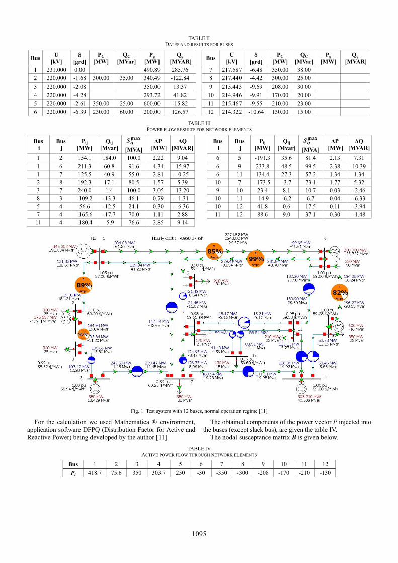
TABLE II DATES AND RESULTS FOR BUSES

Bus U

[kV]

[grd] PC

[MW] QC

[MVar] Pg

[MW] Qg

[MVAR] Bus

U [kV]

[grd]

PC [MW]

QC [MVar]

Pg [MW]

Qg

[MVAR]1 231.000 0.00 490.89 285.76 7 217.587 -6.48 350.00 38.00 2 220.000 -1.68 300.00 35.00 340.49 -122.84 8 217.440 -4.42 300.00 25.00

3 220.000 -2.08 350.00 13.37 9 215.443 -9.69 208.00 30.00

4 220.000 -4.28 293.72 41.82 10 214.946 -9.91 170.00 20.00

5 220.000 -2.61 350.00 25.00 600.00 -15.82 11 215.467 -9.55 210.00 23.00

6 220.000 -6.39 230.00 60.00 200.00 126.57 12 214.322 -10.64 130.00 15.00

TABLE III POWER FLOW RESULTS FOR NETWORK ELEMENTS

Bus i

Bus j

Pij [MW]

Qij [Mvar]

maxijS

[MVA]

ΔP [MW]

ΔQ [MVAR]

Bus

i Bus

j Pij

[MW] Qij

[Mvar]

maxijS

[MVA]

ΔP [MW]

ΔQ [MVAR]

1 2 154.1 184.0 100.0 2.22 9.04 6 5 -191.3 35.6 81.4 2.13 7.31 1 6 211.3 60.8 91.6 4.34 15.97 6 9 233.8 48.5 99.5 2.38 10.39 1 7 125.5 40.9 55.0 2.81 -0.25 6 11 134.4 27.3 57.2 1.34 1.34 2 8 192.3 17.1 80.5 1.57 5.39 10 7 -173.5 -3.7 73.1 1.77 5.32 3 7 240.0 1.4 100.0 3.05 13.20 9 10 23.4 8.1 10.7 0.03 -2.46 8 3 -109.2 -13.3 46.1 0.79 -1.31 10 11 -14.9 -6.2 6.7 0.04 -6.33 5 4 56.6 -12.5 24.1 0.30 -6.36 10 12 41.8 0.6 17.5 0.11 -3.94 7 4 -165.6 -17.7 70.0 1.11 2.88 11 12 88.6 9.0 37.1 0.30 -1.48 11 4 -180.4 -5.9 76.6 2.85 9.14

Fig. 1. Test system with 12 buses, normal operation regime [11]

For the calculation we used Mathematica ® environment, application software DFPQ (Distribution Factor for Active and Reactive Power) being developed by the author [11].

The obtained components of the power vector P injected into the buses (except slack bus), are given the table IV.

The nodal susceptance matrix B is given below.

TABLE IV ACTIVE POWER FLOW THROUGH NETWORK ELEMENTS

Bus 1 2 3 4 5 6 7 8 9 10 11 12

Pi 418.7 75.6 350 303.7 250 -30 -350 -300 -208 -170 -210 -130

1095

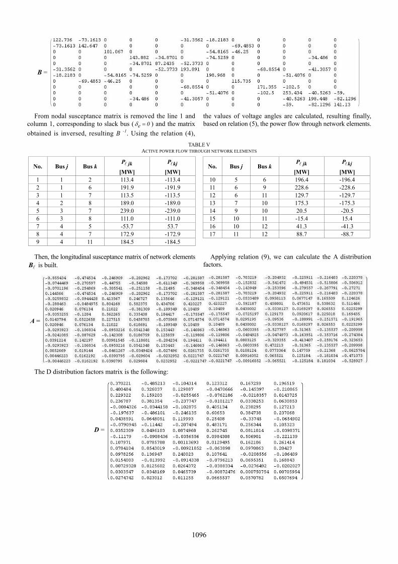
B =

From nodal susceptance matrix is removed the line 1 and column 1, corresponding to slack bus ( e 0 ) and the matrix

obtained is inversed, resulting B -1. Using the relation (4),

the values of voltage angles are calculated, resulting finally, based on relation (5), the power flow through network elements.

TABLE V ACTIVE POWER FLOW THROUGH NETWORK ELEMENTS

No. Bus j Bus k jkP

[MW]

kjP

[MW]

No. Bus j Bus k jkP

[MW]

kjP

[MW] 1 1 2 113.4 -113.4 10 5 6 196.4 -196.4 2 1 6 191.9 -191.9 11 6 9 228.6 -228.6 3 1 7 113.5 -113.5 12 6 11 129.7 -129.7 4 2 8 189.0 -189.0 13 7 10 175.3 -175.3 5 3 7 239.0 -239.0 14 9 10 20.5 -20.5 6 3 8 111.0 -111.0 15 10 11 -15.4 15.4 7 4 5 -53.7 53.7 16 10 12 41.3 -41.3 8 4 7 172.9 -172.9 17 11 12 88.7 -88.7 9 4 11 184.5 -184.5

Then, the longitudinal susceptance matrix of network elements

B is built. Applying relation (9), we can calculate the A distribution

factors.

A =

The D distribution factors matrix is the following:

D =

1096

Using the relation (13) we will be determine the C distribution factors (Table VI).

These factors are calculated only for consumer buses 7, 8, 9, 10, 11 and 12.

TABLE VII THE C DISTRIBUTION FACTORS

Network element j-k Cjk,7 Cjk,8 Cjk,9 Cjk,10 Cjk,11 Cjk,12 1-2 -0.140961 0.280671 -0.217616 -0.196637 -0.206145 -0.202170 1-6 -0.169625 -0.386751 0.001889 -0.0450514 -0.023777 -0.032671 1-7 0.004445 -0.200061 -0.090413 -0.0644521 -0.076218 -0.071299 2-8 -0.196224 0.225408 -0.272879 -0.251900 -0.261408 -0.257433 3-7 -0.030208 -0.105989 -0.254341 -0.227044 -0.324838 -0.283955 3-8 -0.256490 0.745924 -0.304265 -0.319914 -0.384895 -0.357730 4-5 -0.025595 0.035495 0.112308 0.061565 0.051942 0.055965 4-7 0.070066 -0.032962 -0.234654 -0.197543 -0.330500 -0.274916 4-11 -0.266474 -0.224536 -0.099657 -0.086025 0.056554 -0.003052 5-6 -0.208416 -0.147327 -0.070514 -0.121256 -0.130879 -0.126856 6-9 -0.231632 -0.317355 0.150092 -0.064045 -0.242158 -0.167697 6-11 -0.124479 -0.194792 -0.196787 -0.080333 0.109431 0.030099 7-10 -0.427196 -0.313097 0.096571 0.180622 0.026392 0.090868 9-10 0.072534 -0.013189 -0.545741 0.240122 0.062009 0.136470 10-11 -0.014476 0.000885 -0.065639 -0.136062 0.225377 0.074275 10-12 -0.091720 -0.078706 -0.135066 -0.194729 0.111489 0.401528 11-12 -0.098339 -0.111353 -0.054992 0.004671 -0.301547 0.408413

After that it goes on to present the allocation of electricity transmission costs to energy market participants – in our case, for producers and consumers. It is considered as a basis for calculating a unit cost of transport lines 2 $/MW·km.

Total transmission cost was calculated based on unit cost and on the active power flow (Table IV), results being presented in Table 7.

TABLE VIIII THE TOTAL ENERGY TRANSMISSION COST

Bus i

Bus j

Unit transmission cost [$/MW]

Pij [MW]

Total transmission cost [$]

Bus i

Bus j

Unit transmission cost [$/MW]

Pij [MW]

Total transmission cost [$]

1 2 60 113.4 6804 5 6 80 196.4 15712 1 6 140 191.9 26866 6 9 60 228.6 13716 1 7 240 113.5 27240 6 11 100 129.7 12970 2 8 60 189 11340 7 10 80 175.3 14024 3 7 76 239 18164 9 10 40 20.5 820 3 8 90 111 9990 11 10 100 15.4 1540 5 4 120 53.7 6444 10 12 68 41.3 2808.4 4 7 56 172.9 9682.4 11 12 50 88.7 4435 4 11 120 184.5 22140

Total 204695.8

Using D distribution factors, there is determine the transmission costs allocated to generators (Table VIII). Using C distribution

factors, it determines the transmission costs allocated to consumers (Table IX).

TABLE VIII TRANSMISSION COSTS ALLOCATED TO GENERATORS

Cost allocated to generator 1 [$]

Cost allocated to generator 2 [$]

Cost allocated to generator 3 [$]

Cost allocated to generator 4 [$]

Cost allocated to generator 5 [$]

Cost allocated to generator 6 [$]

Total cost [$]

82945.7 9367.1 44195.8 28765.4 39421.8 1832.5 204695.8

TABLE IX TRANSMISSION COSTS ALLOCATED TO CONSUMERS

Cost allocated to consumer 7 [$]

Cost allocated to consumer 8 [$]

Cost allocated to consumer 9 [$]

Cost allocated to consumer 10 [$]

Cost allocated to consumer 11 [$]

Cost allocated to consumer 12 [$]

Total cost [$]

51787.5 29878.9 36137.7 23103.0 38105.1 25683.7 204695.8

1097

Obviously, costs allocation was done separately for sources

(sources share 1, consumers share 0) and consumer (consumer share 1, sources share 0), identifying active power tracing flow. The two components of the transmission cost allocation

can be weighted differently (in the range 01, their sum is obviously 1).

For losses regime it obtained the following results for cost allocated to generators (Table X and Table XI):

TABLE X

TRANSMISSION COSTS ALLOCATED TO GENERATORS (REGIME WITH LOSSES)

Cost allocated to generator 1 [$]

Cost allocated to generator 2 [$]

Cost allocated to generator 3 [$]

Cost allocated to generator 4 [$]

Cost allocated to generator 5 [$]

Cost allocated to generator 6 [$]

Total cost [$]

85001.3 9367.1 44195.8 28765.4 39421.8 1832.5 208583.9

TABLE XI TRANSMISSION COSTS ALLOCATED TO CONSUMERS (REGIME WITH LOSSES)

Cost allocated to consumer 7 [$]

Cost allocated to consumer 8 [$]

Cost allocated to consumer 9 [$]

Cost allocated to consumer 10 [$]

Cost allocated to consumer 11 [$]

Cost allocated to consumer 12 [$]

Total cost [$]

52771.1 30446.4 36824.1 23541.9 38828.8 26171.5 208583.8

IV. CONCLUSION

This paper presents allocation of transmission costs using an extended version of distribution factors methods. The proposed method takes losses into consideration during the calculus process based on the following hypothesis very realistic, especially if one takes into account the lowest share of losses in power flow through network elements. It is considered only change of active power generated in slack bus, distribution factors remaining unchanged.

Regarding the method of distribution factors, applied to 12 nodes test system, it is notable difference of generators and consumers transmission costs allocation, between the cases without and with active power losses.

The recommendation is clear: do not neglect the active power losses.

ACKNOWLEDGMENT

This research is partly supported by the Romanian Power Grid Company “Transelectrica” S.A., in the framework of the research grant UPT No. 658 / 2008.

REFERENCES [1] M.D. Ilic, F.D. Galiana, L.H. Fink, Power Systems Restructuring:

Engineering and Economics, Springer Ltd, 1998. [2] J. Pan, Y. Teklu, S. Rahman, Review of Usage-Based Transmission

Cost Allocation Methods under Open Access, IEEE Transactions on Power System, Vol. 15, No. 4, November 2000, pp. 1218-1224.

[3] Pop O., Nemeş M., Power Transmission Allocation With Network Matrices, The 7th International Power Systems Conference, Timişoara 2007, November 21-23, pp. 527-534.

[4] A.R. Abhyankar, S.A. Soman, S.A. Khaparde, Optimization approach to real power tracing: an application to transmission fixed cost allocation, IEEE Transactions on Power Systems, Vol. 21, No. 3, .August 2006, pp. 1350-1361.

[5] Conejo A.J., Arroyo J.M., Alguacil N., Guijarro A.L., Transmission Loss Allocation: A Comparison of Different Practical Algorithms, IEEE Transactions On Power Systems, Vol. 17, No. 3, August 2002, pp. 571-576.

[6] Tomokazu O., Shuichi K., Shinichi I., Transmission Line Loss Allocation using Power Flow Tracing with Distribution Factors, Power Engineering Society General Meeting, 2007. IEEE, 24-28 June 2007 pp. 1-7.

[7] Ng W.Y., Generalized Generation Distribution Factors for Power System Security Evaluations, IEEE Transactions on Power Apparatus and Systems, Vol. PAS-100, No. 3, March 1981, pp. 1001-1005.

[8] C. Lee, N. Chen, Distribution Factors of Reactive Power Flow in Transmission Line and Transformer Outage Studies, IEEE Transactions on Power Systems, Vol. 7, No. 1, February 1999, pp. 194-200.

[9] Pop O., Paunescu D., Kilyeni St., Nemes M., Kilyeni A., Barbulescu C., Probabilistic Distribution Factors Assessment Using OptimalPowerPrice Mathematica Software. Case Study: Test 25 Buses Test Power System, Proceedings of the 5th International Symposium on Applied Computational Intelligence and Informatics – SACI 2009, May 28-29, 2009, Timisoara, Romania, pp. 453-458.

[10] Shahidehpour M., Yahim H., Li Z., Market Operations in Electric Power Systems. Forecasting, Scheduling and Risk Management, John Wiley & Sons, 2004.

[11] Pop Oana, Contributions on the tariff access assessment to the transport system, PhD Thesis, Faculty of Electrical and Power Engineering, “Politehnica” University of Timisoara, 2009

1098