Transformer Differential Protection Lab · 2016-12-28 · The purpose of the Transformer...

Montana Tech LibraryDigital Commons @ Montana TechProceedings of the Annual Montana Tech Electricaland General Engineering Symposium Student Scholarship

2016

Transformer Differential Protection LabLayne SimonMontana Tech of the University of Montana

Zach KasperickMontana Tech of the University of Montana

Justin DunbarMontana Tech of the University of Montana

Follow this and additional works at: http://digitalcommons.mtech.edu/engr-symposium

This Article is brought to you for free and open access by the Student Scholarship at Digital Commons @ Montana Tech. It has been accepted forinclusion in Proceedings of the Annual Montana Tech Electrical and General Engineering Symposium by an authorized administrator of DigitalCommons @ Montana Tech. For more information, please contact [email protected].

Recommended CitationSimon, Layne; Kasperick, Zach; and Dunbar, Justin, "Transformer Differential Protection Lab" (2016). Proceedings of the AnnualMontana Tech Electrical and General Engineering Symposium. Paper 13.http://digitalcommons.mtech.edu/engr-symposium/13

http://digitalcommons.mtech.edu?utm_source=digitalcommons.mtech.edu%2Fengr-symposium%2F13&utm_medium=PDF&utm_campaign=PDFCoverPages

http://digitalcommons.mtech.edu/engr-symposium?utm_source=digitalcommons.mtech.edu%2Fengr-symposium%2F13&utm_medium=PDF&utm_campaign=PDFCoverPages


http://digitalcommons.mtech.edu/stdt_schr?utm_source=digitalcommons.mtech.edu%2Fengr-symposium%2F13&utm_medium=PDF&utm_campaign=PDFCoverPages


http://digitalcommons.mtech.edu/engr-symposium/13?utm_source=digitalcommons.mtech.edu%2Fengr-symposium%2F13&utm_medium=PDF&utm_campaign=PDFCoverPages

mailto:[email protected]

Transformer Differential Protection Lab

by

Layne Simon, Zach Kasperick, Justin Dunbar

A senior design report submitted in partial fulfillment of the

requirements for the degree of

Electrical Engineering

Montana Tech

2015 -2016

ii

Abstract

The purpose of the Transformer Differential Protection Lab senior design project is to

implement the transformer differential protection scheme to protect a transformer when an

internal fault is applied. Using the Lab-Volt power supply, a Lab-Volt faultable transformer, and

a SEL-787 relay; the transformer differential protection scheme was produced in the Power Lab

found in Main Hall 303. During the project, the SEL-787 was tested for different scenarios that

differential protection could be susceptible to. The scenarios tested were a primary winding-to-

ground fault, an external fault, and harmonics that the transformer may experience during inrush.

The outcomes of the project are to learn about transformer differential protection and produce a

lab procedure that could be used as a future lab for Montana Tech’s Power Protection class.

iv

Table of Contents

ABSTRACT ................................................................................................................................................ II

LIST OF TABLES ....................................................................................................................................... VI

LIST OF FIGURES ..................................................................................................................................... VII

LIST OF EQUATIONS ................................................................................................................................ IX

1. INTRODUCTION ................................................................................................................................. 1

2. SCHEDULE OF PROJECT........................................................................................................................ 2

2.1. Overview of Project ............................................................................................................ 2

2.2. First Semester ..................................................................................................................... 3

2.3. Second Semester ................................................................................................................ 4

3. RESEARCH ........................................................................................................................................ 5

3.1. Faultable Transformer (Chapman, 2012) .................................................................... 5

3.2. Transformer Differential Protection Scheme (Edmund O. Schweitzer, 2010), (Labratories)

10

3.3. Harmonics due to Over-excitation and Inrush Current (Laboratories, 2006-2015) ........ 16

3.4. SEL-787 Relay Settings (Laboratories, 2006-2015) .................................................. 19

4. TESTING AND IMPLEMENTATION ......................................................................................................... 21

4.1. Power Supply Install ......................................................................................................... 21

4.2. Faultable Transformer Parameters/ Ratings ................................................................... 22

4.3. Equipment Setup .............................................................................................................. 24

4.4. Determining Relay Settings .............................................................................................. 27

4.4.1. Single-Slope Operating Characteristic ............................................................................................... 27

4.4.2. Harmonic Blocking ............................................................................................................................. 32

4.5. Testing the Relay .............................................................................................................. 34

4.5.1. Starting the Power Supply ................................................................................................................. 34

v

4.5.2. Normal Operation of the Power System ........................................................................................... 36

4.5.3. Primary Winding-to-Ground Fault Internal to Zone of Protection .................................................... 37

4.5.4. Single Line-to-Ground Fault External to Zone of Protection ............................................................. 39

5. CONCLUSION .................................................................................................................................. 41

5.1. First Semester ................................................................................................................... 41

5.2. Second Semester .............................................................................................................. 42

REFERENCES ........................................................................................................................................... 44

6. APPENDIX A: PROCEDURE FOR TESTING RELAY ...................................................................................... 45

7. APPENDIX B: MATLAB SCRIPT CALCULATING EXPECTED CURRENTS .......................................................... 54

8. APPENDIX C: MATLAB SCRIPT TO COMPARE RESULTS ........................................................................... 56

vi

List of Tables

Table 1: First semester schedule ..........................................................................................4

Table 2: Second semester schedule ......................................................................................5

Table 3: Single Phase Transformer Ratings.......................................................................23

Table 4: Transformer Resistances ......................................................................................23

Table 5: Open Circuit Measurements and Calculations for Normal Operation.................23

Table 6: Open Circuit Measurements for Internal Fault ....................................................24

Table 7: Short Circuit Measurements and Calculations ....................................................24

Table 8: Currents present in normal operation ..................................................................36

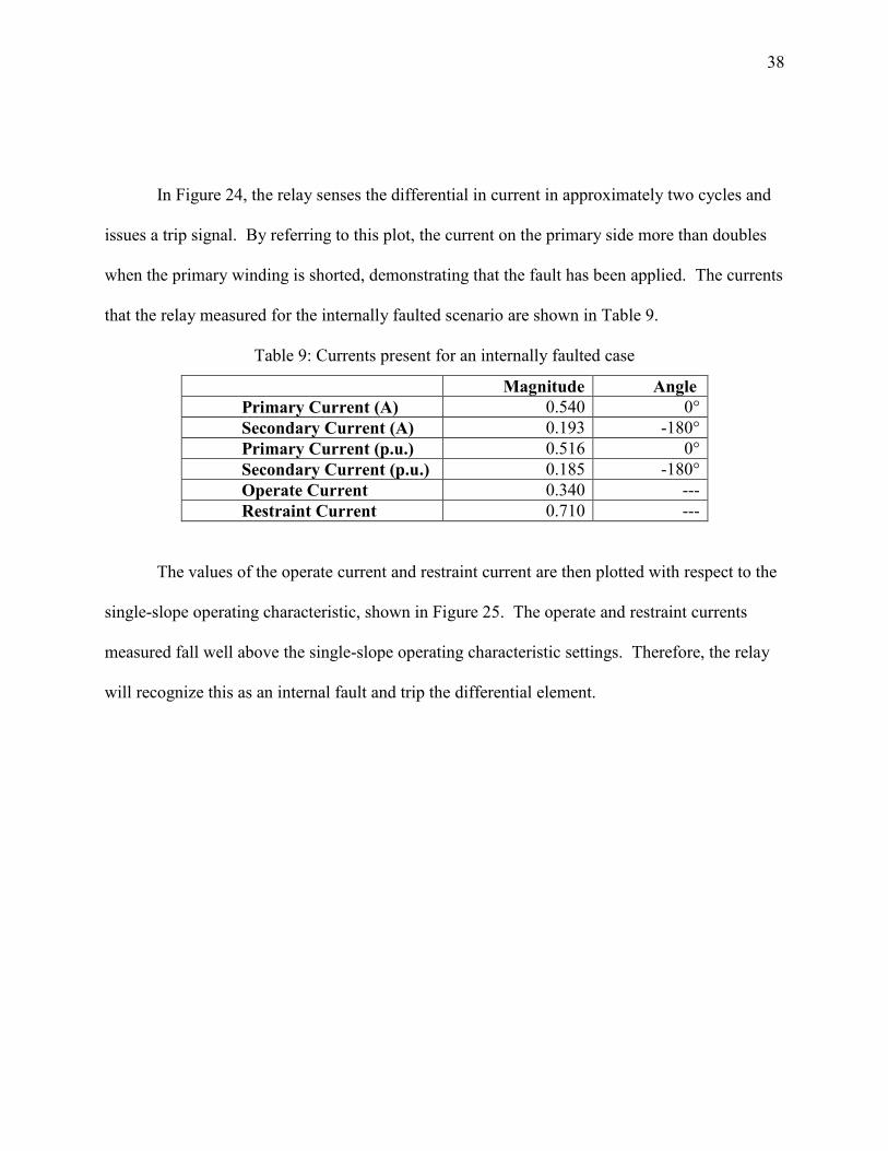
Table 9: Currents present for an internally faulted case ....................................................38

Table 10: External Fault Currents present .........................................................................40

vii

List of Figures

Figure 1: Equivalent Model of Transformer ........................................................................7

Figure 2: Faultable Transformer Module .............................................................................7

Figure 3: Open-Circuit Test .................................................................................................9

Figure 4: Short-Circuit Test .................................................................................................9

Figure 5: Transformer Differential Protection Scheme .....................................................10

Figure 6: Percent Dual-Slope Operating Characteristic.....................................................11

Figure 7: Example of Normal Operation ...........................................................................13

Figure 8: Internal Faulted Condition..................................................................................14

Figure 9: Example of CT Saturation Operation .................................................................15

Figure 10: Harmonic Restraint Example ...........................................................................17

Figure 11: Dual-Slope Operating Curve Setting ................................................................20

Figure 12: California Instruments Power Supply ..............................................................21

Figure 13: Lab-Volt Power Supply Module ......................................................................22

Figure 14: Overview of entire transformer differential set up ...........................................25

Figure 15: Base Case Model used in MATLAB Simulation .............................................28

Figure 16: Internally Faulted Case used in MATLAB Simulation ....................................29

Figure 17: Expected Results for Internal Fault ..................................................................30

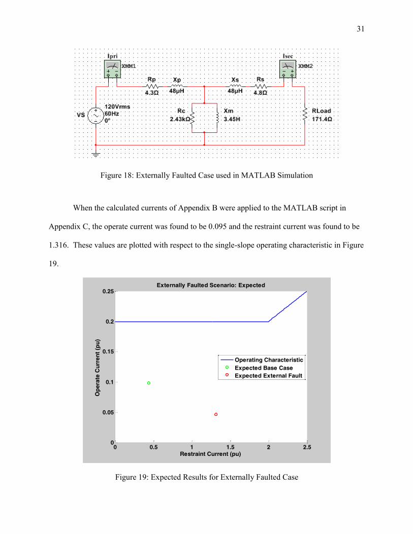
Figure 18: Externally Faulted Case used in MATLAB Simulation ...................................31

Figure 19: Expected Results for Externally Faulted Case .................................................31

Figure 20: Relay Operating for Inrush ...............................................................................33

Figure 21: Harmonics Present During Inrush ....................................................................34

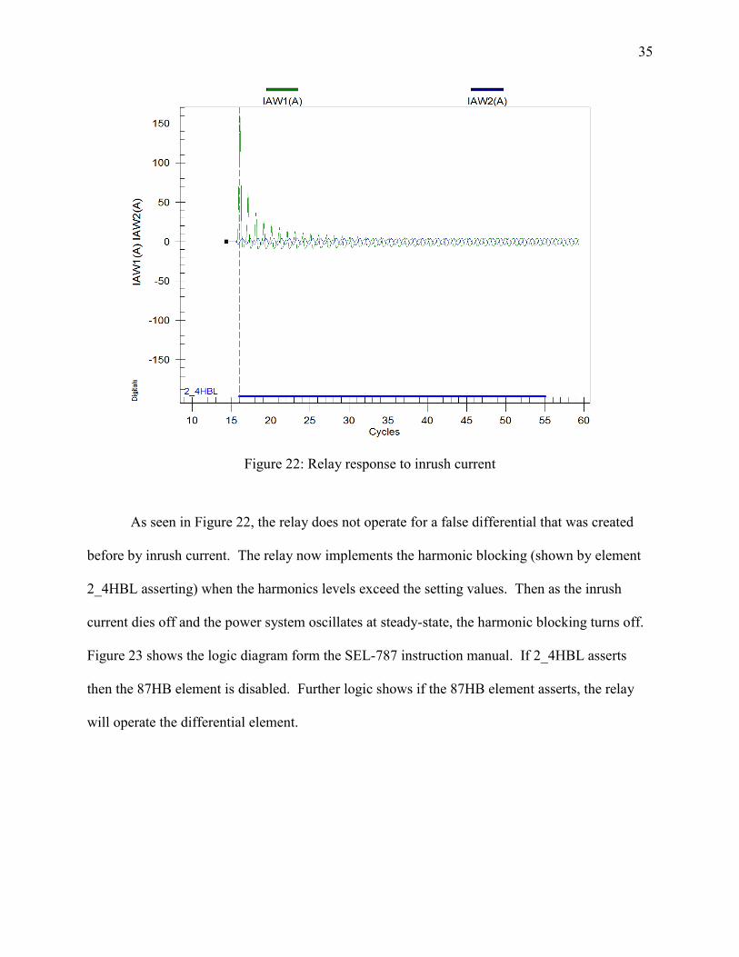
Figure 22: Relay response to inrush current ......................................................................35

viii

Figure 23: Logic Diagram for 2_4HBL .............................................................................36

Figure 24: Event report of the internally faulted scenario .................................................37

Figure 25: Expected verses Actual for Internal Fault ........................................................39

Figure 26: External Fault Expected versus Actual ............................................................40

ix

List of Equations

Equation(1) ..........................................................................................................................6

Equation(2) ..........................................................................................................................6

Equation(3) ..........................................................................................................................6

Equation(4) ..........................................................................................................................8

Equation(5) ..........................................................................................................................8

Equation(6) ..........................................................................................................................8

Equation(7) ..........................................................................................................................8

Equation(8) ..........................................................................................................................8

Equation(9) ........................................................................................................................10

Equation(10) ......................................................................................................................10

Equation(11) ......................................................................................................................11

Equation(12) ......................................................................................................................11

Equation(13) ......................................................................................................................26

Equation(14) ......................................................................................................................26

Equation(15) ......................................................................................................................26

1

1. Introduction

Montana Tech currently offers students the opportunity to take a class that teaches the

fundamentals of power system protection, EELE 456, from two Schweitzer Engineering

Laboratories (SEL) employees, Brian Smyth and Cole Salo. They noticed a demand for a lab

that taught students the principles behind transformer protection. Through the help of team

member Zach Kasperick, whom interned for SEL this past summer, a project was created in

regards to this demand. The goal of this project is to improve the protection class that is offered

to seniors in Electrical Engineering at Montana Tech. Protection of transformers is important in

the power world due to the significant cost of transformers, reliability required by utilities and

expected by their customers, and the safety of the utility workers and the public as a whole.

After successful completion of this project, future students at Montana Tech will receive hands

on experience in the steps and requirements to correctly protect a transformer in a power system

through the current differential protection scheme. Upon conclusion of this project, there will be

four items delivered:

Final paper

Protection scheme lab setup

Poster for the Montana Tech Expo

Presentation for the Senior Symposium

Over the years, different types of power equipment have been donated to Montana Tech.

Some of this equipment is sitting, unused in the “Power” lab located in Main 303. This project

will put this equipment to use and create a lab exercise that provides future students hands on

experience working with transformer current differential protection.

This report covers the results found through the entirety of this project. This includes:

2

Project timeline for first and second semester

Research regarding the faultable transformer module, transformer current

differential protection, harmonics, and relay settings

Results of testing the faultable transformer module to verify relay settings

Having little understanding of protection schemes, this topic required a heavy amount of research

throughout the first semester to understand how transformer current differential protection

works. This is a challenging project that will benefit future students, and provide a strong

foundation for students to succeed in the world of power engineering.

2. Schedule of Project

2.1. Overview of Project

To complete this project, several pieces of equipment were used. The major pieces of

equipment were a Lab-Volt power supply, Lab-Volt faultable transformer module, and a SEL-

787 protection relay. To make this project more manageable, the project was broken up into

smaller steps. The steps taken to complete the project were determined based on the goals that

were set for each semester. The goals for the first semester were determined to be:

Learn the basics of transformer current differential protection

Install power supply in the power lab

Measure the ratings and parameters of the faultable transformer

Present first semester presentation

At the conclusion of the first semester, a presentation was presented to Larry Hunter and

John Morrison that showed the overall status of the project. This served as a time to evaluate the

progress made on the project and decide if scheduling changes were necessary in the second

semester.

3

After the conclusion of the first semester, the project was continued throughout the

second semester. The goals for the second semester were determined to be:

Become familiar with the SEL-787 operation

Calculate relay settings values for transformer current differential protection

Test relay with the faultable transformer

Finish paper with addition of second semester results

2.2. First Semester

For the first semester, the team decided upon three major milestones to achieve the goals

for the semester. The first milestone was to research topics that are applicable to this project.

The first research topic was to review the theory behind transformers. The next research done

was to gain a basic understanding of how transformer protection works. This task entails

research about the topic of transformer current differential protection. The last piece of research

was to learn about the settings to the SEL-787, found in the instruction manual, to protect for

internal faults on a transformer. In order to complete this project, the team must understand how

current differential works and how this is applied to protect a transformer during a faulted

condition.

The second milestone was to install the California Instrument power supply that is

currently in the lab unconnected. This power supply will serve as the power to the faultable

transformer module. To install this supply, a small amount of wiring was done with the help of

Professor Matt Donnelly.

The last milestone was to run tests on the faultable transformer module. Through various

tests, a model of the transformer can be created that will represent various losses. This model

was used during the second semester to help determine the relay settings.

4

In order to ensure completion of the goals outlined for the first semester, a timeline was

set to keep the project on track. The Gantt chart in Table 1 shows the necessary timeline for the

first semester. It can be noted that research was conducted throughout the entire semester and

was therefore not included in the Gantt chart.

Table 1: First semester schedule

2.3. Second Semester

For the second semester, the team decided on four major milestones required for

completion of the project. The first milestone is to research more about the SEL-787 to learn

how to install the relay for operation. This task requires using the instruction manual to learn

how to power the relay and setup communications with the relay using AcSELerator Quickset.

The relay will be tested to ensure correct metering operation.

The second milestone is to calculate the relay settings used to implement a transformer

current differential scheme. The task consists of three counterparts. The first part is to simulate

the fault on the faultable transformer using the parameters found in the first semester. MATLAB

was used as the simulation software. The next is to test the faultable transformer module for

harmonic levels present. The last part is to calculate the settings related to the transformer

current differential protection scheme and apply the setting values to the SEL-787.

Research Task

Determine equipment needed

Setup power source

Setup/test transformer

Prepare and submit progress report.

Present first semester progress

Evaluate schedule of project

20 27 4 11 18 25 1 8 15 22 29 6 13

Dec.Oct. Nov.Sept.

Date of Tasks (by Weeks)

5

The third milestone is testing the relay to ensure it operates correctly with the settings

determined. This task will require an internal and external fault to be applied using the faultable

transformer. The results of the test will be documented to verify the calculated relay settings

used.

The fourth and final milestone of this semester is compiling the deliverables for the

project. The deliverables will all be presented at the Senior Design Symposium that takes place

on April 28th

.

The Gantt chart shown in Table 2, has the expected timeline for the second semester.

The schedule for the second semester was determined based on the progress made during the

first semester, with the deadline for the project the Senior Design Symposium.

Table 2: Second semester schedule

3. Research

3.1. Faultable Transformer (Chapman, 2012)

A transformer is a device that is used to step up or step down the voltages and currents of

a power system. A transformer consists of an input winding and an output winding that are used

to define the turns ratio. Each set of windings have a total number of turns, Np for the primary

side and Ns for the secondary side. Based on these turns, the turns ratio (a) is found by dividing

Research Task

Power SEL-787 w/ SEL QuickSet

Verify correct op/metering of SEL-787

Calculate Relay Setting Values

Implement Full XMFR Diff Prot. Scheme

Corrections to scheme (if necessary)

Prepare project deliverables

Montana Tech Expo/Symposium

10 17 24 31 7 14 21 28 6 13 20 27 3 10 17 24

Jan. Feb. Mar. April

6

the number of turns on the primary side by the number of turns of the secondary, shown in

Equation 1. Once the turns ratio is found, the voltage Vp on the primary side can be related to

voltage Vs of the secondary side by Equation 2. The current Ip of the primary side can also be

related to the current Is with the turns ratio, shown in Equation 3.

a =Np

Ns (1)

a =Vp

Vs (2)

1

a=

Ip

Is (3)

In a real transformer, several imperfections must be taken into consideration to create an

accurate model. The major types of imperfections considered are as follows:

Copper Losses.

Eddy Current Losses.

Hysteresis Losses.

Leakage Flux.

These losses are accounted for with the use of an equivalent circuit of a transformer, as

seen in Figure 1. To model the copper losses, resistive components are added to the primary and

secondary windings of the transformer core. These are shown by resistors labeled Rp and Rs. To

model the leakage flux losses of the transformer, primary and secondary inductors are added.

The inductors are shown with impedance values of Xp and Xs for the primary and secondary

inductors, respectively. The eddy current losses and the hysteresis losses make up the elements

found in the excitation branch of the equivalent circuit. The core current losses are represented

7

with resistor Rc and the core excitation effects are represented with an inductor with an

impedance of Xm.

Figure 1: Equivalent Model of Transformer

For this project, a faultable transformer module is used, seen in Figure 2. This module

will allow for research to be done on the effects of an internal fault on a transformer through the

flipping of a switch.

Figure 2: Faultable Transformer Module

8

For this module, the transformer parameters for the equivalent model of a transformer

were found by using the open-circuit and short-circuit tests. By doing these tests, a reasonable

model of the faultable transformer was found to do testing on.

In order to find the parameters of the equivalent model, two methods are used. The first

method is the open-circuit test, as seen in Figure 3. This involves leaving the secondary winding

of the transformer in an open-circuit, or infinite resistance, while the primary winding is

connected to a full-rated voltage. The open-circuit test is used to find the parameters of the core

modeling the losses of the core. The following equations are used to determine the core

resistance and reactance.

Equation 4 is used to find the no load power factor of the transformer, due to the core

losses. The angle (ө) is solved for and used in degrees.

𝑐𝑜𝑠(ө) =𝑃𝑜𝑐

𝑉𝑜𝑐 ∗ 𝐼𝑜𝑐 (4)

Equation 5 is used to find the current through the resistive element (Iw) in the core. This

value is then used in Equation 6 to solve for the core resistance (Rc).

𝐼𝑤 = 𝐼𝑜𝑐 ∗ cos (ө) (5)

𝑅𝑐 = 𝑉𝑜𝑐

𝐼𝑤 (6)

Equation 7 is used to find the current through the reactive element (Iu) in the core. This

value is then used in Equation 8 to solve for the core reactance (Xm).

𝐼𝑢 = 𝐼𝑜𝑐 ∗ 𝑠𝑖𝑛 (ө) (7)

𝑋𝑚 = 𝑉𝑜𝑐

𝐼𝑢 (8)

9

Figure 3: Open-Circuit Test

The second method is the short-circuit test, as seen in Figure 4. This involves connecting

the secondary side of the transformer short-circuited, or zero resistance, while the primary side is

connected to a variable voltage supply. The voltage is slowly adjusted until the current is equal

to the rated value of the transformer. Because the impedance of the excitation branch is much

larger then series components, a very small amount of current is flowing through the excitation

branch of the transformer and can be ignored. To find the values of Rp and Rs, an ohm meter is

used to measure the resistance of the primary and secondary windings while the power supply is

turned off. After finding these values, Equation 9 and Equation 10 are used to find Xp and Xs on

the primary side of the transformer. Both these methods will be used to determine the

parameters of the faultable transformer.

Figure 4: Short-Circuit Test

10

𝑋𝑝 =

𝑉𝑝

𝐼𝑝−𝑅𝑝+𝑅𝑠𝑎2

2 (9)

𝑋𝑠 = 𝑋𝑝

𝑎2 (10)

3.2. Transformer Differential Protection Scheme (Edmund O. Schweitzer, 2010), (Labratories)

Transformer differential is a protection scheme that can detect faults that occur internally

in a transformer. Current differential protection, shown in Figure 5, works based on the principle

stated by Kirchhoff’s Current Law (KCL) that the sum of the currents flowing into a node is

equal to zero. If the per-unit current on the primary side of the transformer is equal to the per-

unit current on the secondary side of the transformer, then KCL is verified. If KCL is satisfied,

no fault is present and the relay will not operate.

Figure 5: Transformer Differential Protection Scheme

Figure 5 shows a SEL-787 relay connected to the primary and secondary sides of a

transformer. The relay is comparing the per-unit current of the primary side (I1) to per-unit

current of the secondary side (I2). In this scheme, it is standard to have the CT polarity facing

11

away from the differential zone. This results in the two currents, I1 and I2, being 180° out of

phase with each other.

The SEL-787 uses two calculated current values to determine if a fault is present, operate

current (Iop) and restraint current (Irt). To calculate Iop and Irt, Equation 11 and Equation 12 are

used.

𝐼𝑂𝑝 = |𝐼1 + 𝐼2| (11)

𝐼𝑅𝑡 = |𝐼1| + |𝐼2| (12)

Through several relay settings, further discussed in section 3.1.1.4, the percent dual-slope

operating curve, shown in Figure 6, is used to set the operate and restraint region for the relay.

The operate region is the area above the curve where the relay will trip, ideally only when a fault

is present. While the restraint region is the area below the curve where the relay should restrain

from tripping. Using Iop and Irt values the relay can make tripping decisions based off the percent

dual-slope operating curve.

Figure 6: Percent Dual-Slope Operating Characteristic

12

The following three examples demonstrate how the percent dual-slope operating curve

works in regard to Iop and Irt. Example 1 shows Iop and Irt values which plot in the restraining

region signifying no fault is present and the per-unit current on the primary side equals the per-

unit current on the secondary side. Example 2 shows Iop and Irt values which plot in the operating

region, indicating an internal fault to the transformer where the per-unit current on the primary

side no longer equals the per-unit current on secondary side. Example 3 shows how the second

(dual) slope is used to account for CT saturation. When a fault is external to the differential

protection zone, the relay should not operate. External faults can draw a large amount of current,

and if CT’s are not built to withstand the large amount of current present then it will begin to

saturate. If CT values are not equal, it looks like there is differential current present which

results in the relay operation.

Example 1:

I1= 1.0 ∠ 0° per-unit

I2= 1.0 ∠ 180° per-unit

Iop= |1.0 ∠ 0° + 1.0 ∠ 180° | = 0

Irt = |1.0 ∠ 0°| + |1.0 ∠ 180° | = 2

13

Figure 7: Example of Normal Operation

A MATLAB representation of the percent dual-slope operating curve can be seen

in Figure 7. The restraint current is on the x-axis and the operate current is on the y-axis.

The restraining current was calculated to be 2, so this plots 2 in the x-axis. The operate

current is calculated to be 0, and this plots 0 in the y-axis. The red dot represents the

value of (2,0), which are the operate and restraint currents found. The red dot plots in the

restraining region and the relay will not operate for this case as expected.

Example 2:

I1= 1.0 ∠ 0° per-unit

I2= 1.0 ∠ 0° per-unit

Iop= |1.0 ∠ 0° + 1.0 ∠ 0° | = 2

Irt = |1.0 ∠ 0°| + |1.0 ∠ 180° | = 2

14

Figure 8: Internal Faulted Condition

A MATLAB representation of the percent dual-slope operating curve for Example

2 is show in Figure 8. The restraint current is on the x-axis and the operate current is on

the y-axis. The restraining current was calculated to be 2, so this plots 2 in the x-axis.

The operate current was calculated to be 2, and this plots 2 in the y-axis. The red dot

represents the value of (2, 2) which are the operate and restraint currents found. The red

dot plots in the operating region and the relay will operate for this case as expected for an

internal fault.

Example 3:

I1= 3.0 ∠ 0° per unit

I2= 2.2 ∠ 180° per unit

Iop= |3.0 ∠ 0° + 2.2 ∠ 180° | = 0.8

Irt = |3.0 ∠ 0°| + |2.2 ∠ 180° | = 5.2

15

Figure 9: Example of CT Saturation Operation

A MATLAB representation of the percent dual-slope operating curve can be seen

in Figure 9. The restraint current is on the x-axis and the operate current is on the y-axis.

The restraining current was calculated to be 5.2, this plots 5.2 in the x-axis. The operate

current is calculated to be 0.8, and this plots 0.8 in the y-axis. The red dot represents the

value of (5.2, 0.8), which are the operate and restraint currents found. The red dot plots

in the restraining region and the relay’s differential protection scheme will not operate for

this case of CT saturation because the fault is external to the system. Example 3 simply

shows how the percent dual-slope operating curve accounts for cases of CT

saturation. It also can be seen if the single-slope operating characteristic was used for

this same case, the CT saturation may have tripped the relays differential protection zone.

16

When transformer current differential is used to protect transformers, there are several

other factors that need to be considered to ensure correct operation of the relay:

Transformer inrush current when initially energized

Transformer over-excitation

Current Transformer (CT) saturation

CTs are used in large power systems to step down current to an equipment accepted value. In

this project, CTs will not be used because an acceptable amount of current for the SEL-787 is

being used. The rated current for the faultable transformer is 1 amp, therefore less than 1 amp

will be present during normal operations of the power system. For simplicity, the turns ratio of

the faultable transformer used will be 1:1 to avoid unnecessary complications in this project. CT

saturation is accounted for by the second slope on the percent dual-slope operating characteristic.

CT saturation is not an issue in this project because CTs are not used to transform the current,

therefore a single-slope operating characteristic will be used.

3.3. Harmonics due to Over-excitation and Inrush Current (Laboratories, 2006-2015)

Inrush and over-excitation current are two cases that cause a false differential current that

could make the relay operate at unnecessary times. The relay can account for both of these

conditions through the use of harmonics, which are frequency based components. When inrush

current is present, it produces even harmonics which can be detected by the relay. While over-

excitation produces odd harmonics. Harmonic blocking and harmonic restraint are two relay

functions that can be used to protect the relay from tripping for these false differential cases.

Harmonic blocking can be used to make the relay more secure by blocking content that

could cause unwanted operation due to inrush and over-excitation. During harmonic blocking,

the transformer differential protection scheme implemented in the relay is blocked from being

17

able to trip when harmonics are present. For each of the user defined harmonic, the relay blocks

the output differential current if the harmonics magnitude is above the set harmonic percentage

value.

Harmonic restraint will also make the relay more secure. Harmonic restraint uses relay

settings to increase the restraining region of the percent slope operating curve only when

harmonics are present. This is done by adding the amount of the harmonic that is present, to the

restraint current value, shown in Figure 10. This increase moves the value right on the x-axis of

the dual slope operating curve, which in turn will give the relay a higher restraint current value.

The relay now requires more operate current in order to trip. For best security against false

differential, it has been determined that a combination of both harmonic blocking and harmonic

restraint can be used.

Figure 10: Harmonic Restraint Example

18

Inrush current, also called magnetization current, occurs when current is first applied to a

transformer. In this instance, a large amount of current is present on the primary side of the

transformer and produces flux, or magnetization, inside the transformer core. At this instance,

the amount current on the primary side of the transformer will not be equal to the amount of

current on the secondary side of the transformer due to core magnetization. This looks like a

differential current to the relay, which may result in the relay to operate. This case needs to be

accounted for so the relay does not trip for inrush current which is present in all transformers that

are first energized. Inrush current can be detected by 2nd

and 4th

harmonics. These harmonics

can be used to block or restrain the relay from tripping during inrush current.

Over-excitation current occurs when the transformer core begins to saturate. Saturation

of the transformer core is due to overloading the transformer. During over-excitation, the core of

the transformer hits a peak limit in the amount of flux that can be produced. No more flux can

flow through the core once the transformer core is saturated. This will cause a differential

current because some of the current on the transformer’s primary side will not be present on the

secondary side. This case needs to be accounted for so that the relay does not trip for this

condition. Over-excitation current can be detected by the 5th

harmonic. This harmonic can be

used to block or restrain the relay from tripping during over-excitation current.

Part of this project is to determine the harmonics that are produced during various

conditions of inrush and over-excitation. Over-excitation is not tested because in order to

saturate the core of the transformer, current above the transformer ratings must be applied which

could damage the faultable transformer module.

19

3.4. SEL-787 Relay Settings (Laboratories, 2006-2015)

The SEL-787 is a transformer relay that is used to protect the faultable transformer in this

project. Research was conducted to determine some of the possible relay settings that are

required for the SEL-787. These relay settings were determined through use of the SEL-787

instruction manual that was obtained from the SEL website.

The following list displays the settings that were determined in the second semester to

protect the transformer from internal faults and false differential elements using transformer

differential protection:

O87P – Operate current level

SLP1 – Restraint Slope 1

SLP2 – Restraint Slope 2

IRS1 – Intersection point for slope 1 and slope 2.

PCT2 – 2nd

Harmonic Block Value

PCT4 – 4th


PCT5 – 5th


HBLK – Harmonic Block

HRSTR – Harmonic Restraint

The first three on this list are settings that will be used to set the percent differential

operating curve, shown in Figure 11. Through calculations, these settings will be determined in

order for the SEL-787 to operate for the applied amount of current.

20

Figure 11: Dual-Slope Operating Curve Setting

As illustrated in Figure 11, the setting O87P sets the desired pickup of the operating

current value. SLP1 and SLP2 account for steady-state and CT saturation errors that cause false

differential current. Setting SLP1 will start at the origin (0, 0) and intersect at O87P based of the

determined value for SLP1. IRS1 is the intersection point for slope 1 and slope 2, where SLP1

ends and SLP2 begins. The setting of SLP2 must be set greater than or equal to SLP1 value. In

this project, SLP1 will be set equal to SLP2 because the dual-slope operating curve will not be

used to account for CT saturation. When these values are equal, the single-slope operating

characteristic is used.

As previously discussed, harmonics are present during inrush and over-excitation

situations. Relay settings can be set to account for the harmonics present in the faultable

transformer. If harmonic blocking is to be used, relay setting HBLK will be set to ‘Y’ (yes). If

harmonic restraint is to be used, relay setting HRSTR will be set to ‘Y’ (yes). If harmonic

21

blocking is used, the user will determine settings for the PCT2, PCT4, and PCT5 harmonic block

values. These settings are harmonic blocking percentage values for the second, fourth, and fifth

harmonics. If harmonic restraint is used, the user will determine the harmonic restraint values

settings.

During the second semester, relay setting values were determined, along with harmonic

testing to determine the transformer and harmonic settings. Harmonic testing is achieved by

applying the inrush case and using the SEL-787 to capture an event during this case. Capturing

these events requires AcSELerator Analytic to analyze how much harmonics are present. Once

these harmonic percentages are found, it will be decided if harmonic blocking, harmonic

restraint, or both will be used.

4. Testing and Implementation

4.1. Power Supply Install

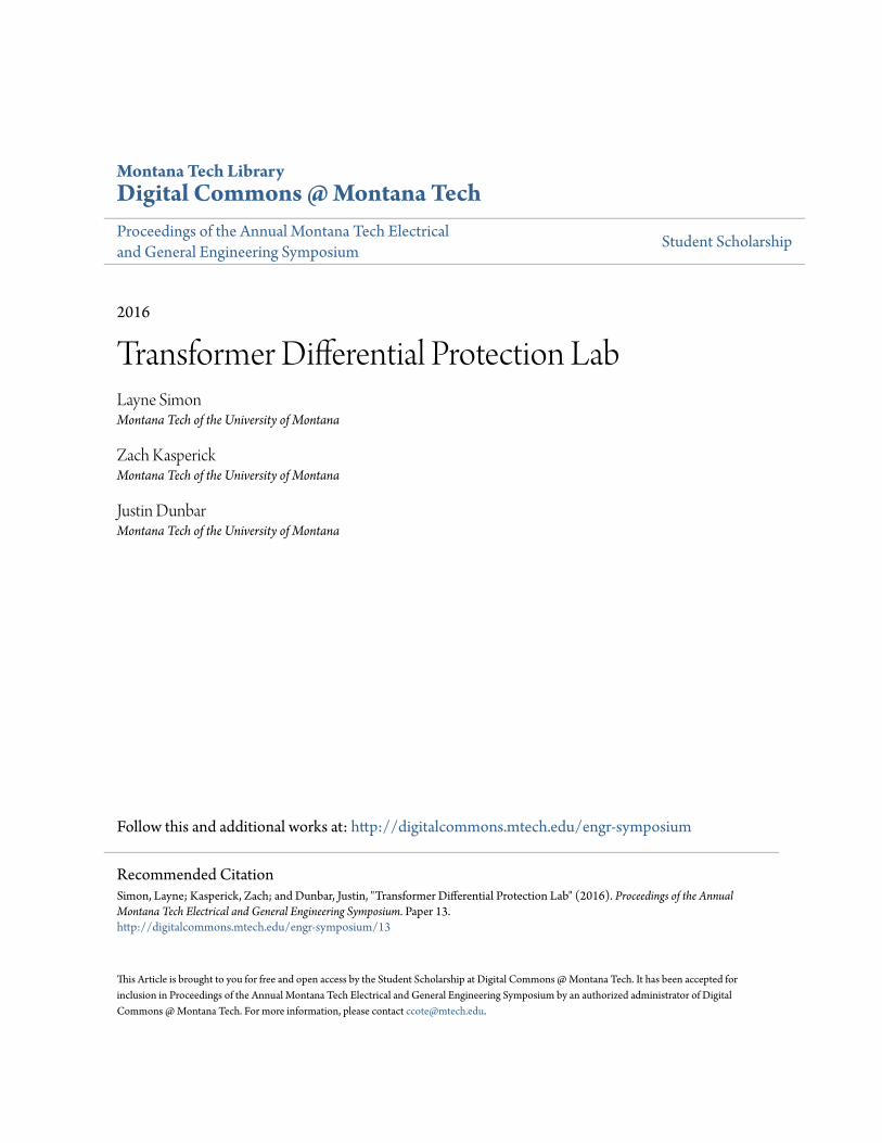
To install the “California Instruments 6000Ls” power supply in Main Hall 303, the team

met with Professor Matt Donnelly, a master electrician. The power supply, shown in Figure 12,

was wired into the electrical wiring of the lab.

Figure 12: California Instruments Power Supply

22

After the power supply was wired, it was tested using a digital multi-meter (DMM) to see

if the power source was outputting the same voltage as the display on the front of the supply.

When the voltage was measured, it was found that the power supplies were working as expected.

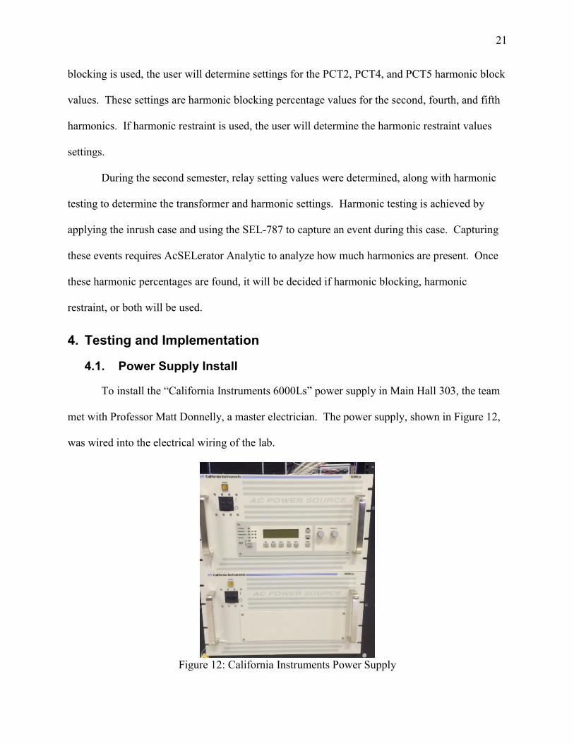
Discussing among ourselves and our mentor, it was determined that using the “Lab-Volt”

power supply, as seen in Figure 13, already mounted on the station would meet the needs

necessary of the power supply to complete the project. This supply is a better option because it

is already mounted next to the transformer and will be able to supply the range of currents that is

needed.

Figure 13: Lab-Volt Power Supply Module

4.2. Faultable Transformer Parameters/ Ratings

In order to accurately model the faultable transformer, the transformer ratings and the

parameter values of the equivalent circuit were found. The first step to do this was to find the

23

ratings of the faultable transformer. The turns ratio used was 1:1 because this project is focusing

on implementing a basic transformer differential protection scheme and an unequal turns ratio

would create unnecessary complexity through the need of additional relay settings. The ratings

seen in Table 3 were found on the front panel of the faultable transformer module.

Table 3: Single Phase Transformer Ratings

Primary Voltage 120 V

Secondary Voltage 120 V

Primary Max Current 1 A

Secondary Max Current 1 A

Turns Ratio (a) 1:1

The next step was to determine the resistance values of the primary and secondary

windings of the transformer. This is done by using a DMM to record the amount of resistance on

each winding when there is no power to the transformer. To find the value of resistance of the

primary winding, the DMM was connecting in parallel to the primary side of the transformer.

This same procedure was followed for the secondary side. The values recorded for the primary

and secondary winding resistance the faultable transformer are shown in Table 4.

Table 4: Transformer Resistances

RP 4.3 Ω

RS 4.8 Ω

The next step was to use the procedure discussed in section 3.1.1.1 of this report on the

open-circuit test on the faultable transformer to determine the values of Rc and Xm. When this

test was completed, the values recorded for the faultable transformer are shown in Table 5.

Table 5: Open Circuit Measurements and Calculations for Normal Operation

Ioc 105 mA

Voc 120.0 V

Poc 5.97 W

Rc 2430 Ω

Xm j1303 Ω

24

The open circuit test again was applied when the switch FS1 was closed, signifying an

internal fault on the primary winding. This shows the core parameters for simulation purposes in

MATLAB. When this test was completed, the values recorded for the core of the faultable

transformer are shown in Table 6.

Table 6: Open Circuit Measurements for Internal Fault

Ioc 359 mA

Voc 120.0 V

Poc 41.8 W

Rc 350 Ω

Xm j1260 Ω

The last step to gather all the parameters needed is to perform the short-circuit test to

determine the values of the series impedances, as discussed in section 3.1.1.1 of this report.

After completion, the values recorded for the primary and secondary winding reactive elements

faultable transformer are shown in Table 7.

Table 7: Short Circuit Measurements and Calculations

IP 0.999 A

VP 9.127 V

XP j0.0181 Ω

XS j0.0181 Ω

The parameters measured for the faultable transformer module were used to simulate this

power system to determine the relay setting that need to be applied to allow the relay to be as

reliable as possible.

4.3. Equipment Setup

In order to implement the transformer current differential protection scheme, a base case

was established to derive normal operation of the SEL-787. Figure 14 shows a model of the base

25

case used for testing. The model shows the connections made to the faultable transformer to

setup the transformer current differential protection scheme for the A-phase.

Figure 14: Overview of entire transformer differential set up

For consistency in testing, a 120 volt fixed voltage source was always used for the

voltage supply. The positive terminal of the voltage source is connected in series to the positive

terminal of IAW1, which is the actual A-phase current that the relay sees. The negative terminal

of IAW1 is then connected to the primary side of the transformer, and the negative of the

primary is connected to ground. Since current transformers are not used for this project, the

secondary side of the transformer is connected to the negative side of the IAW2. By wiring the

secondary current in this manner, the 180 phase shift required for transformer differential

protection is created. The positive terminal of IAW2 was then connected to a 600 Ω load.

Following the 600 Ω load, the transformer was connected to ground.

26

A MATLAB script was created to find the values for the power system being used to test

the faultable transformer. This script can been found in Appendix C of this report. The first part

of this script calculates the per-unit current base so the actual current measurements can be

converted to per-unit. Equations 13 and 14 show equations used to achieve this.

𝐼𝐵𝑎𝑠𝑒 = 𝑆𝐵𝑎𝑠𝑒

√3∗𝑉𝐵𝑎𝑠𝑒,𝐿𝐿 (13)

𝐼𝑝𝑢 =𝐼𝑚𝑒𝑎𝑠𝑢𝑟𝑒𝑑

𝐼𝐵𝑎𝑠𝑒 (14)

The second part of this script establishes the ratings of the power system such that a TAP

value can be calculated to get a normalized current on the primary and secondary side of the

transformer, shown in Equation 15. When the actual ratings of the transformer were used, it

resulted in the TAP value to not fall in the acceptable range needed for operation. To get a TAP

value that would be acceptable, the parameters MVA, VWDG, and CTRn were adjusted until the

calculated TAP value was approximately 1.0. A TAP of 1.0 was desired because the TAP value

in this power system accounts only for the 1:1 turns ratio in the transformer.

The TAP ratio uses several different values to get a normalized current value. MVA is

the maximum power transformer capacity (in MVA) and was set to 5 MVA. VWDG is the

winding line-to-line voltage setting (in kV) and was set to 138 kV. The n specifies the winding

being set (1-Primary, 2-Secondary). CTRn is the current transformer ratio setting and was set

equal to 20 for both primary and secondary. The C was set to 1, since the transformer does not

have phase or magnitude offset from a delta-wye connection. It can be noted again that these

values are not the same as the actual ratings of the faultable transformer model.

𝑇𝐴𝑃𝑛 = 𝑀𝑉𝐴 ∗ 1000

√3 ∗ 𝑉𝑊𝐷𝐺 ∗ 𝐶𝑇𝑅𝑛∗ 𝐶 (15)

27

4.4. Determining Relay Settings

4.4.1. Single-Slope Operating Characteristic

The first relay setting determined to acquire the single-slope operating characteristic is

the pickup current value, O87P. To find this value, the power system being studied is modeled

using MATLAB. By using this software, it is possible to determine the amount of current to

expect in three scenarios: normal operation, internal fault, and external fault. The MATLAB

script for each of the scenarios is located in Appendix B.

The first scenario simulated is the normal operation of the power system. This scenario is

very important in determining the O87P element because this will reveal the amount of operate

current to expect in the power system during normal operation periods. To model the power

system in MATLAB, there are several components needed. The first component to model is the

faultable transformer module. This can be achieved by using the equivalent model of the

transformer (using the parameters found in Section 4.2 of this report). The model consists of the

primary resistance (Rp), primary inductance (Xp), core resistance (Rc), and core inductance (Xm).

The secondary resistances were then reflected to the primary side, the secondary resistance (Rs)

and secondary inductance (Xs). The turns ratio is set be 1:1 in this instance to simulate the base

case. The secondary side values were then reflected to the primary side of the transformer using

this turns ratio. The next component to model is the voltage supply. An AC Source is used with

the voltage set to 120 Vrms. Finally, the last component is the load that is being supplied. For

this, a resistor with a resistance of 600 is used and is also reflected to the primary side of the

transformer. After setting up the model, the simulation can be ran to find the current on the

primary and secondary sides under normal conditions. Figure 15 shows a model of the base

case. XMM1 and XMM2 signifies the SEL-787 relay connections of IAW1 and IAW2

respectively.

28

Figure 15: Base Case Model used in MATLAB Simulation

When the calculated currents of Appendix B were applied to the MATLAB script in

Appendix C, the operate current was determined to be 0.098 and the restraint current was found

to be 0.437. This MATLAB script converts these measurements into per-unit values that can be

used to determine the amount of operate and restraint current in this scenario.

The second scenario simulated is an internal fault to the primary winding of the

transformer, which requires the same setup as the base case. To apply the primary winding-to-

ground fault simulation (that is available on the faultable transformer module by closing FS1),

the parameters found in section 4.2 for the internally faulted case were applied. The faulted case

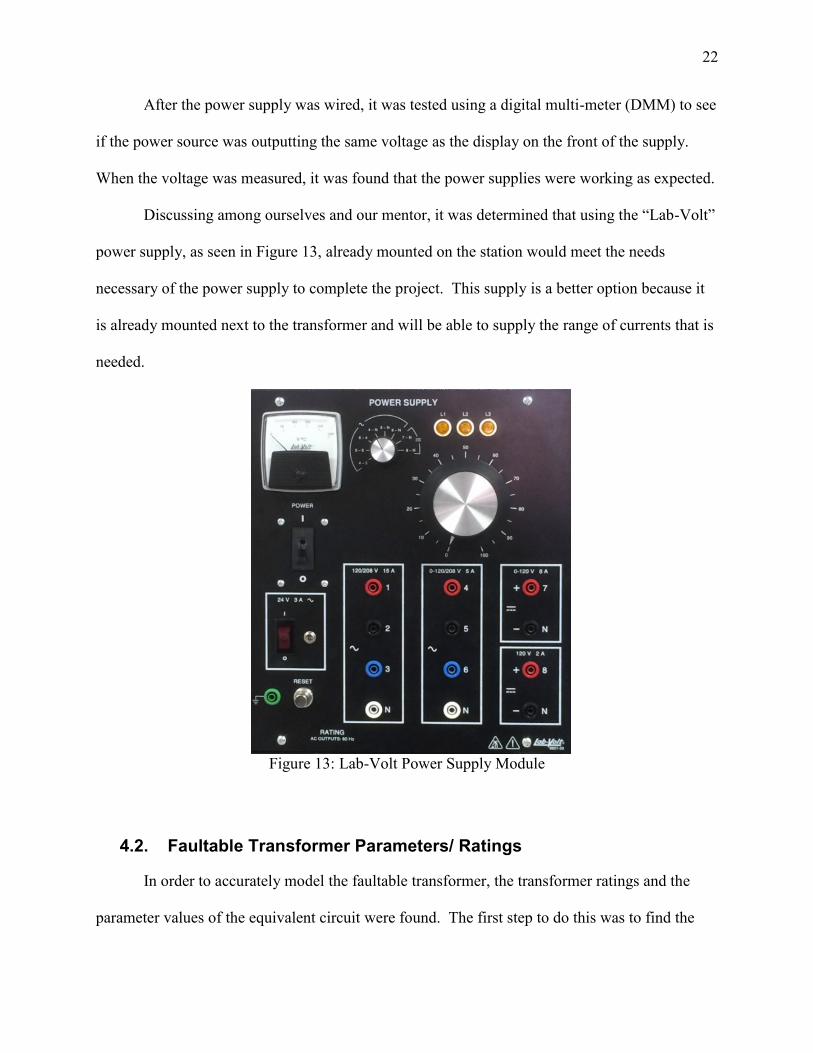
model that was used for the internally faulted simulation is shown in Figure 16.

29

Figure 16: Internally Faulted Case used in MATLAB Simulation


Appendix C, the operate current was determined to be 0.327 and the restraint current was found

to be 0.690. By comparing the increase in operate current, it was determined to set the O87P

element to 0.20. By setting this value nearly twice the operate current of the base case, the relay

will be more secure for errors experienced in testing that may result in the operate current in the

base case being larger than expected. SLP1 was then determined to be set to 10% for this case to

account for possible equipment errors. The slope is set to a low rating because equipment errors

are expected to be small and not be a huge factor in this project. SLP2 was also set to 10%,

because current transformers are not used and CT saturation is therefore not an issue. IRS1 was

left as the default value of 6 because the two slopes are set equal to each other. Figure 17 shows

the single-slope operating characteristic created by these relay settings and the location of the

base and internally faulted scenarios.

30

The third and final scenario is an external fault. This is accomplished by applying a

single line-to-ground fault on the load. The single line-to-ground fault is simulated by lowering

the resistive load. There will be three resistors added in parallel to acquire a lower equivalent

resistance. Since the resistor banks have three resistance values available, the three resistors will

be 1200 , 600 , and 300 in parallel which gives and equivalent resistance of 171.4 .

Figure 18 shows the model used to run this MATLAB simulation.

Figure 17: Expected Results for Internal Fault

0 0.5 1 1.5 2 2.50.05

0.1

0.15

0.2

0.25

0.3

0.35

0.4Internally Faulted Scenario: Expected

Restraint Current (pu)

Op

era

te C

urr

en

t (p

u)

Operating Characteristic

Expected Base Case

Expected Internal Fault

31

Figure 18: Externally Faulted Case used in MATLAB Simulation


Appendix C, the operate current was found to be 0.095 and the restraint current was found to be

1.316. These values are plotted with respect to the single-slope operating characteristic in Figure

19.

Figure 19: Expected Results for Externally Faulted Case

0 0.5 1 1.5 2 2.50

0.05

0.1

0.15

0.2

0.25Externally Faulted Scenario: Expected


Op

era

te C

urr

en

t (p

u)


Expected Base Case

Expected External Fault

32

4.4.2. Harmonic Blocking

The next settings to acquire for the relay are the harmonic blocking percentages for the

2nd

and 4th

harmonics. These settings can be critical in a relay because they block the relay from

operating due to inrush current. In order to find the percentage of these element, a test was done

that demonstrated the harmonics present at the initial startup of the power supply in our power

system.

In order to complete this experiment, the first step is to turn settings PCT2, PCT4, and

harmonic blocking OFF. By deactivating these settings, the harmonic blocking element will not

help the relay restrain from tripping during startup of the power supply.

The next step is to discharge the flux of the core. This is a critical step in this test

because if the core is not correctly discharged, flux will remain in the core and the full effect of

inrush current will not be experienced by the system. To do this, simply connect a resistive load

in parallel with the primary winding of the faultable transformer. This will allow the flux built

up in the core to be dissipated through the resistor.

Finally, the last step is to turn the power on. When the power supply is energized, the

relay will see a large spike in current due to inrush that may cause a large enough differential in

current to cause the relay to operate. If the relay does not operate, then the core of the

transformer is not large enough to create a false differential and the harmonic blocking would

therefore not be necessary for this project. However, it would still be acceptable to apply the

harmonic blocking to increase the security of the relay.

This test procedure was applied to the power system for this experiment, shown in Figure

20. When the power supply was started, the relay tripped in two cycles (33.3 milli-sec) due to

large amount of inrush current. Therefore, this test proves that our relay must be equipped with

harmonic blocking to keep the relay from operating due to inrush current.

33

Figure 20: Relay Operating for Inrush

Now that it has been determined that inrush will cause problems if ignored, the

percentage of the 2nd

and 4th

harmonic need to be determined. By using the harmonic analyzing

tool in AcSELerator Analytic, the harmonics the relay experienced at any given time during an

event report can be found. This tool will allow the harmonics to be viewed at the moment before

the inrush current dies off and the system reaches normal operation. The results of using the

harmonic analyzer are show in Figure 21.

34

Figure 21: Harmonics Present During Inrush

Based on Figure 21, the settings for PCT2 and PCT4 were found to be 20% and 10%

respectively. By applying these settings, the relay should not operate due to inrush current. This

test is explained in further detail in Appendix A.

4.5. Testing the Relay

4.5.1. Starting the Power Supply

When the power supply in the power system was turned on, the primary side of the

transformer experienced a large inrush of current which tripped our differential element. To fix

this problem, harmonic blocking was used in the relay to block the 2nd

and 4th

harmonic once

they reached a percentage of the fundamental frequency (60Hz). When these relay settings were

implemented along with our differential protection settings, the relay was able to avoid operating

on startup of the power supply, as seen in Figure 22.

35

Figure 22: Relay response to inrush current

As seen in Figure 22, the relay does not operate for a false differential that was created

before by inrush current. The relay now implements the harmonic blocking (shown by element

2_4HBL asserting) when the harmonics levels exceed the setting values. Then as the inrush

current dies off and the power system oscillates at steady-state, the harmonic blocking turns off.

Figure 23 shows the logic diagram form the SEL-787 instruction manual. If 2_4HBL asserts

then the 87HB element is disabled. Further logic shows if the 87HB element asserts, the relay

will operate the differential element.

36

Figure 23: Logic Diagram for 2_4HBL

Based on this test, it is verified that the harmonic block setting used are acceptable for

the faultable transformer. The relay asserts harmonic blocking as soon as the inrush current is

experienced, then when the inrush current is gone the harmonic blocking is de-asserted.

Therefore, by using harmonic blocking the problems associated with inrush current is avoided.

Because harmonic blocking worked as expected, we decided that this should be used to account

for inrush, therefore harmonic restraint was not used.

4.5.2. Normal Operation of the Power System

Now that the relay will account for inrush current, the next test is to view the power

system during normal operation. For this test, there were not any faults applied to the power

system. This test is used to determine how close the MATLAB model is to the actual system.

When the system was built in the lab, the values in Table 8 were found.

Table 8: Currents present in normal operation

Magnitude Angle

Primary Current (A) 0.255 0°

Secondary Current (A) 0.195 -162°

Primary Current (p.u.) 0.249 0°

Secondary Current (p.u.) 0.186 -162°

Operate Current 0.092 ---

Restraint Current 0.435 ---

37

By comparing these values to the MATLAB results, it was observed that the operate

current and restraint currents were very accurate and the results matched closely as expected.

This test verified that the relay settings are valid for this case as the relay does not operate for the

base case.

4.5.3. Primary Winding-to-Ground Fault Internal to Zone of Protection

The next step is to apply a fault internal to the transformer differential zone of protection.

This fault is a primary winding-to-ground fault that is applied by closing FS1 on the faultable

transformer module. When the fault is applied, the LED that signifies a differential trip on the

front of the SEL-787 illuminates. The event report, graphed using AcSELerator Analytic, of this

internally faulted scenario is shown in Figure 24.

Figure 24: Event report of the internally faulted scenario

38

In Figure 24, the relay senses the differential in current in approximately two cycles and

issues a trip signal. By referring to this plot, the current on the primary side more than doubles

when the primary winding is shorted, demonstrating that the fault has been applied. The currents

that the relay measured for the internally faulted scenario are shown in Table 9.

Table 9: Currents present for an internally faulted case

Magnitude Angle







The values of the operate current and restraint current are then plotted with respect to the

single-slope operating characteristic, shown in Figure 25. The operate and restraint currents

measured fall well above the single-slope operating characteristic settings. Therefore, the relay

will recognize this as an internal fault and trip the differential element.

39

Figure 25: Expected verses Actual for Internal Fault

This case verifies the relay operates as expected for the internal fault applied to the

transformer, and that the relay settings are valid for this case.

4.5.4. Single Line-to-Ground Fault External to Zone of Protection

To further validate these settings, an externally faulted scenario was simulated. An

external fault should not cause the relay to operate since the fault is not taking place inside the

differential zone of protection. To simulate an external fault, the load resistance was decreased

to approximately 170 Ω, thus simulating a single line-to-ground on near the load. This is

achieved by placing the 1200 Ω resistor, 600 Ω resistor, and 300 Ω resistors, of the resistor bank

module, in parallel to represent the load on the secondary side of the transformer. As the load

resistance is decreased, the current will increase simulating a signal line-to ground fault. Table

10 shows currents that were measured for the externally faulted scenario.

0 0.5 1 1.5 2 2.50.05

0.1

0.15

0.2

0.25

0.3

0.35

0.4Internally Faulted Scenario: Expected versus Actual


Op

era

te C

urr

en

t (p

u)


Expected Base Case

Expected Internal Fault

Actual Base Case

Actual Internal Fault

40

Table 10: External Fault Currents present

Magnitude Angle







For the externally faulted scenario, the operate current remained very close to that of the

base case, while the restraint current saw a large increase. Due to these behaviors of the operate

and restraint quantities, the relay does not operate for this fault because it falls outside of the

operate region of the single-slope operating characteristic. The values for the operate and

restraint currents are plotted in regards to the MATLAB expectations in Figure 26. It can be

seen that the values of the MATLAB vs the actual case were again very close as expected.

Figure 26: External Fault Expected versus Actual

0 0.5 1 1.5 2 2.50

0.05

0.1

0.15

0.2

0.25Externally Faulted Scenario: Expected versus Actual


Op

era

te C

urr

en

t (p

u)


Expected Base Case

Expected External Fault

Actual Base Case

Actual External Fault

41

This faulted scenario demonstrates why an external relay would be used to detect and

isolate the fault. This may allow the transformer to be kept in service once the external fault is

isolated by the out of zone relay. The results obtained from this test demonstrated that the relay

settings used worked well for the different tests.

5. Conclusion

5.1. First Semester

The overall progress of the first semester went according to the expected schedule. All of

the major milestones were met for the first semester, and did not impact the second semester

schedule. The major tasks that were completed in the first semester include:

Research on Transformer Differential

Power supply needed for the project

Parameters for the Lab Volt faultable transformer module

Research of transformer differential protection was completed through meetings with our

mentor, Brian Smyth, the SEL-787 instruction manual, and the Modern Solutions for Protection,

Control, and Monitoring of Electric Power Systems book. Through these resources, principles of

transformer differential protection were learned.

One issue in the first semester consisted of installing the California Instruments power

supply. This power supply was expected to be used for the project, but further research proved

the Lab-Volt power supply module served a more practical use for this project. The Lab-Volt

power supply produced a more practical range of currents that is needed for this project based on

the parameters determined for the faultable transformer. The California Instruments power

supply has a much larger range of currents and could damage the equipment if too much current

is applied. For this reason, the Lab-Volt power supply was selected as the power supply since it

42

was already installed and will be easier to connect to the SEL-787 relay and faultable

transformer module.

The last milestone for the first semester was to complete the open-circuit and short-circuit

test to find the parameters of the faultable transformer. These parameters allow for an accurate

model of the faultable transformer to be created which is used during the second semester to

calculate the desired relay settings.

5.2. Second Semester

For the second semester four milestones were determined in order to complete the project

prior to the Montana Tech Symposium. The four milestones that were completed in the second

semester were:

Install SEL-787 for testing and verify correct metering of relay.

Calculate relay settings used to implement transformer differential protection scheme.

Testing the relay to verify correct relay settings were used.

Complete senior design poster, paper, and prepare presentation for MT Tech Symposium.

The installation of the SEL-787 was completed earlier than scheduled. For completion of

this task, the relay was found to meter the same current values as the Lab-Volt Data acquisition

module. This is explained more in Appendix A.

The calculation of relay settings was completed by using the faultable transformer parameters

found in the first semester. The values of the expected operate and restraint currents were found

using MATLAB. Once the expected values were found, the settings were determined using the

SEL-787 instruction manual. The relay settings were calculated by the scheduled time.

Testing to verify the relay settings were correct consisted of applying an inrush case, internal

fault, and external fault. The first test was to verify correct harmonic settings, which was tested

43

by applying inrush current and verifying that the relay is blocked from tripping. The second test

was to apply an internal fault. When this fault was applied, the relay tripped as expected and the

results were documented. The final test was to apply an external fault to verify the relay did not

trip for an out of zone fault. Again, the relay operated as expected. The testing portion took the

most time but was completed without impacting the expected project schedule.

The final milestone was to complete all documents prior to the deadline. The documents

completed consisted of the Senior Design Poster, Symposium Presentation, and Senior Design

Paper. The paper includes a procedure that allows replication of setup and tests performed

throughout the semester. This procedure can be turned into a lab or multiple labs containing

Transformer Differential Protection. Overall, the documents were completed on time.

For an addition to this project, other protection schemes (such as overcurrent or directional

schemes) could also be implemented. There is also more that can be added to transformer

differential, such as restricted earth fault detection.

By testing the SEL-787, the students in the group became familiar with using a relay and

protection scheme that is used across the nation and world to protect transformers. Having this

knowledge, the students will be much more prepared for working in the field of power systems.

44

References

Chapman, S. J. (2012). Electric Machine Fundamentals Fifth Addition. New York, NY: McGraw

Hill.

Edmund O. Schweitzer, I. a. (2010). Moder Solutions for Protection, Control, and Monitoring of

Electric Power Systems. Pullman, WA 99163: Schweitzer Engineering Laboratories,

INC.

Laboratories, S. E. (2006-2015). SEL-787 Transformer Protection Relay Instruction Manual.

Schweitzer Engineering Laboratories .

45

6. Appendix A: Procedure for Testing Relay

Initial Setup

Part 1. Set up the faultable transformer module for differential current protection.

1. Place faultable transformer into Lab-Volt Station.

2. Connect output of 120 V A-phase power supply to positive terminal of current I1

in the Data Acquisition and Control Interface (DAC).

3. Connect negative terminal of current I1 from the DAC to the positive terminal of

IAW1 of the SEL-787.

4. Connect negative terminal of IAW1 to the positive primary winding of

Transformer P2, this is labeled as T1 P2 on the faultable transformer module.

5. Connect the negative terminal of the primary winding of Transformer P2 to the

neutral of the power supply.

6. Connect the positive winding of the secondary side (S2) to the negative terminal

of IAW2 on the SEL-787. This creates the 180 degree phase shift required for

differential protection in the relay.

7. Connect the negative terminal of the secondary winding of Transformer P2 to the

neutral of the power supply.

8. Connect the positive terminal of IAW2 to the positive terminal of I2 on the DAC.

9. Connect the negative terminal of the I2 current on the DAC to the top of the

resistive load. Close the 600 ohm resistance on the resistive load to set the load

resistance.

10. Connect the bottom of the 600 ohm resistance to neutral.

Refer to connection diagram below for setup. (Note: The DAC is referred to as XMM1

(I1) and XMM2

46

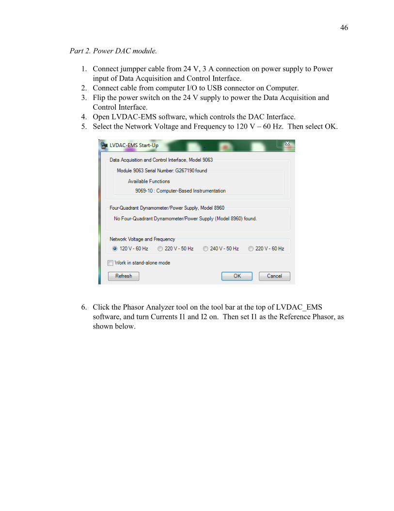
Part 2. Power DAC module.

1. Connect jumpper cable from 24 V, 3 A connection on power supply to Power

input of Data Acquisition and Control Interface.

2. Connect cable from computer I/O to USB connector on Computer.

3. Flip the power switch on the 24 V supply to power the Data Acquisition and

Control Interface.

4. Open LVDAC-EMS software, which controls the DAC Interface.

5. Select the Network Voltage and Frequency to 120 V – 60 Hz. Then select OK.

6. Click the Phasor Analyzer tool on the tool bar at the top of LVDAC_EMS

software, and turn Currents I1 and I2 on. Then set I1 as the Reference Phasor, as

shown below.

47

Part 3. Setup relay communications.

1. Open up AcSELerator Quickset.

2. Click on the tab Communications > Parameters, which is found on the top of

Quickset. Select the Active Connection Type as serial. Under Device, select the

correct COM port that is connected to the SEL-787. Then select the correct Baud

rate (default 9600). Then click Connect.

48

3. Click Communication > Terminal to open up terminal window.

4. Get to the level 2 security level and insert the settings shown below by issue a

SET command.

49

Testing

Part 1. Normal operation

1. Make sure all switches on the faultable transformer are open, then turn the power

supply on.

2. Go to the LVDAC- EMS software and verify the I1 current is approximately 0.25

∠ 0° A and I2 is 0.19 ∠ 169° A.

3. In terminal window, verify the currents IAW1 and IAW2 are a magnitude of the

CTR greater than the actual from above (I1*CTR) by issuing a MET command.

4. Verify IOP1 = 0.09 per-unit and IRT1= 0.43 per-unit by issuing a MET DIFF

command, as shown below.

50

Part 2. Primary winding-to-ground fault (Internal fault).

1. While running at normal operation, activate switch FS1 on T1. This will apply a

primary winding-to-ground fault on the transformer.

2. Verify the LVDAC-EMS software sees a current value of 0.54 ∠ 0° A and 0.19∠

171° A, as shown below.

51

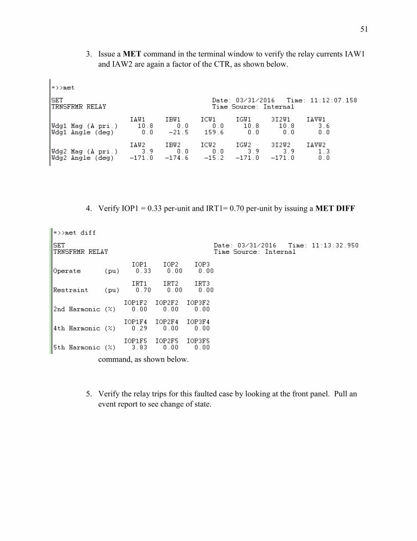
3. Issue a MET command in the terminal window to verify the relay currents IAW1

and IAW2 are again a factor of the CTR, as shown below.



5. Verify the relay trips for this faulted case by looking at the front panel. Pull an

event report to see change of state.

52

Part 3. Single line-to-ground fault on the load (External fault).

1. To simulate a single line-to ground fault, decrease the load resistance to

approximately 170 ohms. This can be achieved by adding the 1200 ohm, 600

ohm, and 300 ohm resistors in parallel.

2. View the results in the LVDAC software.

53

3. Issue a MET command in the terminal window to verify the relay currents IAW1

and IAW2 are again a factor of the CTR, as shown below



5. This verifies that an external fault was applied because the IRT current increases

but the IOP current remains constant.

Part 4. Harmonic Inrush Current

1. Completely power off the system.

2. Issue a SET R and change the event report length to 64 cycles (which is the

maximum amount of time. Then change the pre-fault time to 15 cycles, which will

allow the event to capture data 15 cycles before the event is triggered.

3. Pull this event report as a raw CEV in order to view the harmonics. Verify the

2_4HBLK element asserts in the relay word bits.

54

7. Appendix B: MATLAB Script Calculating Expected Currents

%% Senior Design: Power System Expectations % Authors: Layne Simon, Zach Kasperick, Justin Dunbar % Mentor: Brian Smyth % Date: 04-09-2016

% This code takes the parameters measured from the faultable transformer % module and calculates the expected primary and secondary currents % for the three faulted scenarios.

clear all; close all; clc;

%% Constants of Power System Vs = 120; % Power Supply Voltage a = 1; % Transformer Turns Ratio

Req = 9.1; % Rp + a^2*Rs Xeq = 1i*0.036; % Xp + a^2*Xs

%% Case 1. Normal Operation of the Power System (Base Case) Rc_Base = 2429; % Eddy Current Losses of Core Xm_Base = 1i*1303; % Hysteresis Losses of Core Rload_Base = 600;

Zp_Base = Req + Xeq; Zc_Base = (Rc_Base*Xm_Base)/(Rc_Base+Xm_Base);

Zpar_Base = (Zc_Base*Rload_Base)/(Zc_Base+Rload_Base); Ztot_Base = Zp_Base + Zpar_Base;

IAW1_base = Vs/Ztot_Base; % Primary Current IAW2_base = -Vs*(Zpar_Base/Ztot_Base)/Rload_Base; % Secondary Current

%% Case 2. Primary Winding-to-Ground Fault (Internal Fault) Rc_Int = 350; Xm_Int = 1i*1260; Rload_Int = 600;

Zp_Int = Req + Xeq; Zc_Int = (Rc_Int*Xm_Int)/(Rc_Int+Xm_Int);

Zpar_Int = (Zc_Int*Rload_Int)/(Zc_Int+Rload_Int); Ztot_Int = Zp_Int + Zpar_Int;

IAW1_int_Flt = Vs/Ztot_Int; % Primary Current IAW2_int_Flt = -Vs*(Zpar_Int/Ztot_Int)/Rload_Int; % Secondary Current

%% Case 3. Single Line-to-Ground Fault (External Fault) Rc_Ext = 2429; Xm_Ext = 1i*1303; Rload_Ext = 171.4;

55

Zp_Ext = Req + Xeq; Zc_Ext = (Rc_Ext*Xm_Ext)/(Rc_Ext+Xm_Ext);

Zpar_Ext = (Zc_Ext*Rload_Ext)/(Zc_Ext+Rload_Ext); Ztot_Ext = Zp_Ext + Zpar_Ext;

IAW1_ext_Flt = Vs/Ztot_Ext; % Primary Current IAW2_ext_Flt = -Vs*(Zpar_Ext/Ztot_Ext)/Rload_Ext; % Secondary Current

%% Save Variables to be used in Appendix C. save('Calculated_Currents.mat', 'IAW1_base', 'IAW2_base',... 'IAW1_int_Flt', 'IAW2_int_Flt',... 'IAW1_ext_Flt', 'IAW2_ext_Flt')

56

8. Appendix C: MATLAB Script to Compare Results

%% Senior Design: Single-Slope Operating Characteristic % Authors: Layne Simon, Zach Kasperick, Justin Dunbar % Mentor: Brian Smyth % Date: 04-09-2016

% This script is used to calculate the amount of operate current and % restraint current experienced by the relay for three cases.

% The first case was called the base case. In this case, the normal % operation of the power system was determined.

% The second case simulated an internal fault that shorts 50% of the % primary winding of the transformer to ground.

% The third case demonstrates an external fault. In this case, a single % line to ground fault is simulated near the load.

% For each case, the value of the restraint versus operate current was % plotted on a single-slope operating characteristic to show if the relay % should operate.

clear all; close all; clc;

%% Power System Constants MVA = 5*10^6; % Apparent power base CTR1 = 20; % Primary CT ratio CTR2 = 20; % Secondary CT ratio Vbase = 138*10^3; % Voltage base Ibase = MVA/(sqrt(3)*Vbase); % Current base

%% TAP Ratio Calculations for Primary and Secondary Sides of the XFMR TAP1 = (MVA)/(sqrt(3)*Vbase*CTR1); TAP2 = (MVA)/(sqrt(3)*Vbase*CTR2); fprintf('TAP1 = %.2f\n', TAP1) fprintf('TAP2 = %.2f\n\n', TAP2)

%% Case 1. Normal Operation of the Power System (Base Case) % Power System Expectations load('Calculated_Currents.mat') % Import Calculated Currents

I1pu_base = IAW1_base*CTR1/Ibase; % Per-unit primary current I2pu_base = IAW2_base*CTR2/Ibase; % Per-unit secondary current

Irt_base = (abs(I1pu_base)+abs(I2pu_base)); % Calculating restraint current Iop_base = abs(I1pu_base+I2pu_base); % Calculating operate current

fprintf('Base Case: Iop = %.3f pu, Irt = %.3f pu\n', Iop_base, Irt_base)

% Results from Lab Testing IAW1_base_Lab = 0.258; % Actual Primary Current

57

IAW2_base_Lab = -0.184 - 1j*0.061; % Actual Secondary Current

I1pu_base_Lab = IAW1_base_Lab*CTR1/Ibase; % Per-unit primary current I2pu_base_Lab = IAW2_base_Lab*CTR2/Ibase; % Per-unit secondary current

Irt_base_Lab = (abs(I1pu_base_Lab)+abs(I2pu_base_Lab)); % Calculating

restraint current Iop_base_Lab = abs(I1pu_base_Lab+I2pu_base_Lab); % Calculating operate

current

fprintf('Lab Base Case: Iop = %.3f pu, Irt = %.3f pu\n\n', Iop_base_Lab,

Irt_base_Lab)

%% Case 2. Primary Winding-to-Ground Fault (Internal Fault) % Power System Expectations I1pu_int_Flt = IAW1_int_Flt*CTR1/Ibase; % Per-unit primary current I2pu_int_Flt = IAW2_int_Flt*CTR2/Ibase; % Per-unit secondary current

Irt_int_Flt = (abs(I1pu_int_Flt)+abs(I2pu_int_Flt)); % Restraint current Iop_int_Flt = abs(I1pu_int_Flt+I2pu_int_Flt); % Operate current fprintf('Internally Faulted Case: Iop = %.3f pu, Irt = %.3f pu\n', ... Iop_int_Flt, Irt_int_Flt)

% Results from Lab Testing IAW1_int_Flt_Lab = 0.545; % Actual primary current IAW2_int_Flt_Lab = -0.193 - 1i*0.029; % Actual secondary current

I1pu_int_Flt_Lab = IAW1_int_Flt_Lab*CTR1/Ibase; % Per-unit primary current I2pu_int_Flt_Lab = IAW2_int_Flt_Lab*CTR2/Ibase; % Per-unit secondary current

Irt_int_Flt_Lab = (abs(I1pu_int_Flt_Lab)+abs(I2pu_int_Flt_Lab)); % Restraint

current Iop_int_Flt_Lab = abs(I1pu_int_Flt_Lab+I2pu_int_Flt_Lab); % Operate

current fprintf('Lab Internally Faulted Case: Iop = %.3f pu, Irt = %.3f pu\n\n', ... Iop_int_Flt_Lab, Irt_int_Flt_Lab)

%% Case 3. Single Line-to-Ground Fault (External Fault) % Power System Expectations I1pu_ext_Flt = IAW1_ext_Flt*CTR1/Ibase; % Per-unit primary current I2pu_ext_Flt = IAW2_ext_Flt*CTR2/Ibase; % Per-unit secondary current

Irt_ext_Flt = (abs(I1pu_ext_Flt)+abs(I2pu_ext_Flt)); % Restraint current Iop_ext_Flt = abs(I1pu_ext_Flt+I2pu_ext_Flt); % Operate current

fprintf('Externally Faulted Case: Iop = %.3f pu, Irt = %.3f pu\n', ... Iop_ext_Flt, Irt_ext_Flt)

% Results from Lab Testing IAW1_ext_Flt_Lab = 0.713; % Actual primary current IAW2_ext_Flt_Lab = -0.659 - 1j*0.067; % Actual secondary current

I1pu_ext_Flt_Lab = IAW1_ext_Flt_Lab*CTR1/Ibase; % Per-unit primary current I2pu_ext_Flt_Lab = IAW2_ext_Flt_Lab*CTR2/Ibase; % Per-unit secondary current

58

Irt_ext_Flt_Lab = (abs(I1pu_ext_Flt_Lab)+abs(I2pu_ext_Flt_Lab)); % Restraint

current Iop_ext_Flt_Lab = abs(I1pu_ext_Flt_Lab+I2pu_ext_Flt_Lab); % Operate

current

fprintf('Lab Externally Faulted Case: Iop = %.3f pu, Irt = %.3f pu\n\n', ... Iop_ext_Flt_Lab, Irt_ext_Flt_Lab)

%% Single-Slope Operating Characteristic O87P = 0.20; % Minimum Iop level for operation SLP1 = 0.10; % SLP1: 10% Irt = 0:0.01:4; % Irt axis y = zeros(1,length(Irt)); % Calculating single-slop characteristic inter = O87P/SLP1; % Intersection point

for ii = 1:length(Irt) if Irt(ii) < inter y(ii) = O87P; else y(ii) = SLP1*Irt(ii); end %if else end %for

%% Plots Included in the Paper figure(1) hold on plot(Irt, y) % Operating Characteristic plot(Irt_base, Iop_base, 'go') % Expected Base Case plot(Irt_int_Flt, Iop_int_Flt, 'ro') % Expected Internally Faulted Case

title('Internally Faulted Scenario: Expected') xlabel ('Restraint Current') ylabel ('Operate Current') legend('Operating Characteristic', 'Expected Base Case', ... 'Expected Internal Fault', 'Location', 'SouthEast')

figure(2) hold on plot(Irt, y) % Operating Characteristic plot(Irt_base, Iop_base, 'go') % Expected Base Case plot(Irt_ext_Flt, Iop_ext_Flt, 'ro') % Expected Externally Faulted Case

title('Externally Faulted Scenario: Expected') xlabel ('Restraint Current') ylabel ('Operate Current') legend('Operating Characteristic', 'Expected Base Case', ... 'Expected External Fault', 'Location', 'East')

figure(3) hold on plot(Irt, y) % Operating Characteristic plot(Irt_base, Iop_base, 'go') % Expected Base Case plot(Irt_int_Flt, Iop_int_Flt, 'ro') % Expected Internally Faulted

Case

59

plot(Irt_base_Lab, Iop_base_Lab, 'kx') % Actual Base Case plot(Irt_int_Flt_Lab, Iop_int_Flt_Lab, 'mx') % Actual Internally Faulted Case

title('Internally Faulted Scenario: Expected versus Actual') xlabel ('Restraint Current') ylabel ('Operate Current') legend('Operating Characteristic', 'Expected Base Case', ... 'Expected Internal Fault', 'Actual Base Case', ... 'Actual Internal Fault', 'Location', 'SouthEast')

figure(4) hold on plot(Irt, y) % Operating Characteristic plot(Irt_base, Iop_base, 'go') % Expected Base Case plot(Irt_ext_Flt, Iop_ext_Flt, 'ro') % Expected Externally Faulted

Case plot(Irt_base_Lab, Iop_base_Lab, 'kx') % Actual Base Case plot(Irt_ext_Flt_Lab, Iop_ext_Flt_Lab, 'mx') % Actual Externally Faulted Case

title('Externally Faulted Scenario: Expected versus Actual') xlabel ('Restraint Current') ylabel ('Operate Current') legend('Operating Characteristic', 'Expected Base Case', ... 'Expected External Fault', 'Actual Base Case', ... 'Actual External Fault', 'Location', 'East')

figure(5) hold on plot(Irt, y, 'k') % Operating Characteristic plot(Irt_base, Iop_base, 'rd','linewidth',4) % Expected Base

Case plot(Irt_int_Flt, Iop_int_Flt, 'kd','linewidth',4) % Expected

Internally Faulted Case plot(Irt_ext_Flt, Iop_ext_Flt, 'bd','linewidth',4) % Expected

Externally Faulted Case plot(Irt_base_Lab, Iop_base_Lab, 'r*','linewidth',4) % Actual Base Case plot(Irt_int_Flt_Lab, Iop_int_Flt_Lab, 'k*','linewidth',4) % Actual

Internally Faulted Case plot(Irt_ext_Flt_Lab, Iop_ext_Flt_Lab, 'b*','linewidth',4) % Actual

Externally Faulted Case

title('Results: Expected versus Actual') xlabel ('Restraint Current') ylabel ('Operate Current') legend('Operating Characteristic', 'Expected Base Case', ... 'Expected Internal Fault', 'Expected External Fault', ... 'Actual Base Case', 'Actual Internal Fault', ... 'Actual External Fault', 'Location', 'NorthEast') axis([0 2.5 0 0.4])

figure(6) plot(Irt, y, 'k') title('Single-Slope Operating Characteristic') xlabel ('Restraint Current') ylabel ('Operate Current') axis([0 4 0 0.4]

Transformer Differential Protection Lab · 2016-12-28 · The purpose of the Transformer...

Documents

Transcript of Transformer Differential Protection Lab · 2016-12-28 · The purpose of the Transformer...