University of Arkansas, FayettevilleScholarWorks@UARK

Theses and Dissertations

5-2016

Trade and Transport in Late Roman SyriaChristopher Wade FletcherUniversity of Arkansas, Fayetteville

Follow this and additional works at: http://scholarworks.uark.edu/etd

Part of the Archaeological Anthropology Commons, Geographic Information SciencesCommons, Near and Middle Eastern Studies Commons, Remote Sensing Commons, and the Socialand Cultural Anthropology Commons

This Thesis is brought to you for free and open access by ScholarWorks@UARK. It has been accepted for inclusion in Theses and Dissertations by anauthorized administrator of ScholarWorks@UARK. For more information, please contact scholar@uark.edu.

Recommended CitationFletcher, Christopher Wade, "Trade and Transport in Late Roman Syria" (2016). Theses and Dissertations. 1594.http://scholarworks.uark.edu/etd/1594

Trade and Transport in Late Roman Syria

A thesis submitted in partial fulfillment of the requirements for the degree of

Master of Arts in Anthropology

Christopher Fletcher University of Arkansas Fayetteville

Bachelor of Arts in Anthropology Spring 2013 Bachelor of Arts in History Fall 2013

May 2016 University of Arkansas

This thesis is approved for recommendation to the Graduate Council

Dr. Jesse Casana Thesis Director

Dr. Kenneth L. Kvamme Committee Member

Dr. Wesley D. Stoner Committee Member

Abstract

Despite the relative notoriety and miraculous level of preservation of the Dead Cities of

Syria, fundamental questions of economic and subsistence viability remain unanswered. In the

1950s Georges Tchalenko theorized that these sites relied on intensive olive monoculture to

mass export olive oil to urban centers. Later excavations discovered widespread cultivation of

grains, fruit, and beans which directly contradicted Tchalenko’s assertion of sole reliance on

oleoculture. However, innumerable olive presses in and around the Dead Cities still speak to a

strong tradition of olive production. This thesis tests the logistical viability of olive oil

transportation from the Dead Cities to the distant urban centers of Antioch and Apamea.

Utilization of Raster GIS and remote sensing data allows for the reconstruction of the physical

and social landscapes of Late Roman Syria. Least Cost Analysis techniques produce a

quantitative and testable model with which to simulate and evaluate the viability of long

distance olive oil trade. This model not only provides a clearer understanding of the nature of

long distance trade relationships in Syria, but also provides a model for investigating ancient

economic systems elsewhere in the world. Furthermore, this project allows for the generation

of new information regarding sites that are currently inaccessible to researchers.

Acknowledgements

I would like to express my sincere gratitude to my committee for their support and

invaluable feedback on this project. Special thanks are due to my advisor Dr. Jesse Casana for

assistance selecting and refining this research topic. I also owe a heartfelt thanks to all of my

graduate colleagues in the University of Arkansas department of Anthropology. Without their

feedback and support this project would have been much the lesser. Finally I owe special

thanks to Karen Pownall, my steadfast editor. Without her aid this project would have been

impossible.

Dedication

This Thesis is dedicated to my whole family. Without your unwavering support, I could

have never made it so far.

Table of Contents

I. Chapter One: Introduction…………………………………………………………………………………………….1

II. Chapter Two: Background……………………………………………………………………………………………..7

a. What Makes a Dead City.........................................................................................9

b. Olive Oil in the Late Roman Period……………………………………………………………………13

c. Discussion………………………………………………………………………………………………………..18

III. Chapter Three: Locational Analysis of the Dead Cities……………..…………………………………..20

a. Remote Sensing Methods…………………………………………………………………………………25

b. Method One: Georeferencing Existing Maps to Guide Site Prospection……………26

c. Method Two: Crowdsourcing Site Location with Google Earth………………………...30

d. Method Three: Brute Force Method……..………………………………………………………….35

e. Conclusions from Site Location…………………………………………………………………………36

IV. Chapter Four: Reconstruction of the Late Roman Landscape……………………………………….40

a. Roman Roads……………………………………………………………………………………………………42

b. Hydrology…………………………………………………………………………………………………………48

c. Topography……………………………………………………………………………………………………...54

d. Settlements……………………………………………………………………………………………………...54

e. Conclusions……………………………………………………………………………………………………...56

V. Chapter Five: Least Cost Path Model Construction……………………………………………………....58

a. Considering the Construction of the Model………………………………………………………60

b. Rasterized Data………………………………………………………………………………………………..60

c. Creation of Slope Layer…………………………………………………………………………………….61

d. Reclassification of Data…………………………………………………………………………………….62

e. Compositing the Base Layers into Friction and Cost Layers……………………………….64

f. Conclusions………………………………………………………………………………………………………70

g. Other Observations from the Models……………………………………………………………….72

VI. Chapter Six: Olive Oil Case Study………………………………………………………………………………….75

a. The Olive Oil Trade……………………………………………………………………………………………75

VII. Chapter Seven: Conclusions………………………………………………………………………………………….80

a. Settlement Density……………………………………………………………………………………………80

b. Discussion of the Models………………………………………………………………………………….82

c. Economic Implications………………………………………………………………………………………89

d. Abandonment…………………………………………………………………………………………………..92

e. Conclusions………………………………………………………………………………………………………93

VIII. References…………………………………………………………………………………………………………………..94

IX. Appendix 1…………………………………………………………………………………………………………………101

1

Chapter One: Introduction

The exact nature and scale of ancient economies are, and have long been, fiercely

debated in history, anthropology, and more recently, archaeology. There is no shortage of texts

by economists or historians discussing ancient economics, but these sources rarely integrate

archaeological data into their analyses (e.g. Weber 1905, 1927; Marx 1964; Frank 1933-40;

Polanyi 1957a 1957b; 1963; Finley 1977). For decades, any debate regarding ancient economies

was dominated by conflicting tendencies which either viewed past economic behavior as

similar, albeit more simplistic version of our own, or a radically different creature altogether

(Smith 2004). For the bulk of the later twentieth century, ancient economies in general, and the

ancient Greek and Roman economies in particular, have served as a battle ground for these

fundamentally different models of past economic behavior. This dichotomy of views was chiefly

expressed in history and archaeology as the primitivist vs modernist debate.

For decades influential primitivist scholars expressed the tendency to view ancient

economies as fundamentally different economic systems by highlighting “the small-scale,

agrarian orientation, and stagnant nature of ancient economic activities” (Smith 2004: 75).

Moses Finley’s persuasive primitivist writings dominated the bulk discussion of ancient

economics for decades (Finley 1999). However, as historical and archaeological research

progressed, higher levels of economic activity than previously suspected became increasingly

clear. On the back of this new data, and in opposition to primitivist thought, modernists felt

that the differences between ancient economies are our own economic systems were a matter

of scale, not of type (Smith 2004).

2

The “same versus other” conundrum was expressed slightly differently in economic

anthropology. In economic anthropology this propensity to polarize past economies took the

form of the formalist and substantivist schools of thought. Similar to the modernists, formalists

argued that ancient economies and non-capitalist economies differ only slightly from capitalist

economies. Whereas substantivists posit that ancient and non-capitalist economies are

radically different from modern capitalist economies. The economic anthropologist Karl Polanyi

was amongst the most outspoken substantivists. Polanyi’s work provided a number of

fascinating insights into economic inquiry. However Polanyi’s firm rejection of any possible

capitalistic factors in non-capitalistic economies has limited exploration of these fruitful topics.

Polanyi felt that reciprocity and redistribution were the key factors that drove past economic

behavior. While these ideas are not without merit, reciprocity and redistribution cannot fully

explain the variety of economic production and specialization evident in the archaeological

record (Decker 2001, 2009). When confronted with new data regarding the scale and

specialization of past economies, Polanyi’s model could not satisfactorily reconcile these new

data. The rigidness of Polanyi’s models can be exposed by his rejection of the concept of

“prices” (Polanyi 1957). Polanyi held that equivalencies, set by royal decree, permanently fixed

the value of tradable goods.

The age old debates between modernists/primitivists and formalists/substantivists,

though perhaps not as widely debated now, still cast a major shadow on modern economic

scholarship. The eloquent and persuasive rejection of capitalistic elements of the ancient

economy from imposing scholars like Finley and Polanyi still forms a baseline for much of the

discussion of ancient economics. Lost in the length and breadth of these debates was the role

3

that archaeological data could play. The above debates were largely driven by historical data

and economic theoreticians. While these sources provide much fodder for interesting

discussion, archaeology is ideally poised to help further elucidate ancient economic systems.

Despite its utility, only relatively recently have archaeologists begun to apply the wealth of

relevant data gleaned from survey and excavation (Greene 1986; Harris 1993; Smith 2004).

A single case study, such as Late Roman Syria, is unlikely to resolve the decades old

debate of modernists versus primitivists, but it can provide invaluable insight into the operation

of an ancient economy.1 In his conclusions, Greene cites transportation as “...the key to

defining the physical limits to trade” (Greene 1986: 169) Discussion of transport in Roman trade

is far from novel, however earlier scholars tended to treat speed of movement (e.g. walking,

marching, or cart speed) as the main factor in travel (Casson 1974). While speed of travel is an

important factor, other physical factors such as access to roads, topography, and the presence

of hydrological features all play an important role in the relative ease of trade.

Ancient economies defy easy description and direct examination. However,

archaeological evidence and specific case studies can provide fascinating glimpses into the

experiences of long past economies. This thesis will examine a specific element of economic

activity in the highlands of northwestern Syria. Through a detailed examination of the nature

and extent of Late Roman olive oil trade in the limestone massif region of Syria, the degree and

1 Here and throughout this project the “Late Roman” will be used in lieu of “Byzantine” or “Late Antique.”

4

landscape of the greater Late Roman economy can begin to be addressed.2 This thesis utilizes

remote sensing and Geographical Information Systems (GIS) to reconstruct the physical and

cultural landscape of Late Roman Syria. From these data, a testable Least Cost Path (LCP) model

is then created. Utilizing technical GIS model building allows for the creation of testable and

repeatable datasets that can be examined both quantitatively and qualitatively (White and

Surface-Evans 2012; White and Barber 2012). Such a model tests the logistical viability of the

regional olive oil trade. Relative viability is tested against contemporaneous lowland

settlements. These settlements, located in the neighboring lowland valleys, allow for the direct

comparison of accumulated cost of travel and trade. These contemporary lowland sites are,

geographically speaking, much closer to the urban centers. Given this proximity, it can be

assumed that travel to and from these sites would be less costly. The cost of travel to and from

these lowland sites forms a baseline against which travel cost from the Dead Cities can be

tested. If the olive oil trade is found to be viable then larger conclusions of interregional trade

and economic structures can be examined. If the olive oil trade of northwestern Syria is not

logistically viable then its role in interregional trade can be viewed as exaggerated and

inaccurate.

This thesis is divided into seven chapters. The first chapter is this introduction of the

methods, goals, and scope of this thesis. The second chapter provides a much more thorough

background of the archaeological research and landscape of the limestone massif in Syria. The

2 Limestone massif is a collective physiographic term applied to five limestone hill ranges in northwestern Syria. I will refer to this geological formation as the “limestone massif” or more simply the “massif.”

5

second chapter will trace the history of archaeological discovery and thought in northwest Syria

and highlight some of the critical ambiguities that still remain in modern scholarship.

Chapter three will describe the remote sensing methods used to locate and study the

Dead Cities. Determining the location of the Dead Cities proved to be anything but

straightforward. As such, a number of distinct methods were utilized to compile a dataset

containing a significant number of these sites. Chapter three will also discuss the issues and

accuracies of remote sensing in the limestone massif region.

Chapter four discusses the digital reconstruction of the Late Roman physical and cultural

landscape of the limestone massif region. Multiple aspects of the landscape were studied with

the intent of translating them into the final model. These aspects include topography,

hydrology, wetland marshes, settlement patterns and road networks. This process hinged on

determining which features of the landscape were present during the Late Roman period. As

such, the modern landscape was viewed as a palimpsest that, though reused, still contained

indelible traces of the Late Roman landscape (Casana 2003). Chapter four also discusses the

textual and digital sources drawn upon to interpret and integrate the Late Roman landscape.

Chapter five discusses the reconstruction of the Least Cost Path model itself. First the

base layer data (discussed in chapter four) must be properly formatted and weighted. Once

created, the LCP model allows for the drawing of some initial observations. These initial findings

are briefly discussed. A simple test of the model’s construction is performed at the end of

chapter five to validate that the model has interpreted the data correctly.

6

Chapter six provides a framework for the scale and value of the oil surpluses potentially

produced in the limestone massif region. This chapter quantified the hypothetical oil surplus

based on an agricultural model proposed by Decker (Decker 2009). Chapter six then discusses

some of the archaeological evidence that supports oil export from the Dead Cities.

The findings of this thesis are discussed in full in chapter seven. The initial observations

from the previous chapters are addressed in light of the findings of the full model. The exertion

required to move trade goods from the sites themselves to the nearby urban centers is

quantified and discussed. The results of this chapter illustrate how the Dead Cities fit into the

fabric of the wider eastern Mediterranean trade. In addition, the findings of this thesis can shed

new light on the age old questions of economic life in the Dead Cities, and their eventual

abandonment. Ultimately, these findings allow the opportunity to reevaluate the long standing

debates regarding the nature of the Late Roman economy.

7

Chapter Two: Background

The complex landscape of Northwestern Syria is fascinating in its own right. Steep

rugged Jebels (an Arabic term for mountain or hill) rise high above the perfectly flat Amuq and

Ghab agricultural plains. The Jebels Wastani, Il A’la, Barisha, Sim’an, and Zawiye collectively

form the limestone massif. The limestone massif stands roughly between 400 and 800 meters

above sea level. Though this is not high compared with the Amanus Mountains to the north,

from the perspective of the flat plains, the Jebels dominate the horizon. To see the rough

windswept expanses of the Jebels today, one would be hard pressed to imagine that such a

landscape, at one time, supported a flourishing Late Roman countryside.

The limestone massif region receives comparatively sparse rainfall, between 300-600

mm per year (Casana 2014). The soil on the massif is thin, poor, and rocky. Even in the modern

era, the Jebel highlands have remained an underpopulated hinterland. Only quite recently has

population and development begun to increase here. The topography of the Jebels is broken

and cut with steep and narrow wadis. This broken physical landscape renders travel difficult

and time consuming. Despite all of these factors, dotting the massif every one or two

kilometers are some of the most intact examples of Late Roman architecture, village life, and

religious structures in the world today. Collectively, these marvelously preserved structures are

known to Western scholarship as “The Dead Cities.”3 In reality, the Dead “Cities” are actually

agglomerations of hundreds of villages, monasteries, pilgrimage sites, and farmsteads. The

misleading term “Le Ville Mort” was coined by the early French antiquarian Charles-Melchior-de

3 Despites its limitations, the term “Dead Cities” or “Dead Cities Sites” will be used to

collectively describe these sites.

8

Vogue (de Vogue 1865-77). These sites all date from the Roman or Late Roman Periods 100 B.C.

to A.D. 600, and there is little evidence for settlement previous to these periods (Foss 1996).

Due in part to their astonishing level of preservation, the Dead Cities have come to lead the

discussion of the Roman/Late Roman countryside (e.g. Decker 2009; Wickham 2005). Prior to

the current political upheaval in Syria, the Dead Cities were a tourist mainstay. Daily trips left

from Aleppo and allowed tourist to step backward in time (Beattie and Pepper 2001). In 2011

these stunning sites were collectively proclaimed a UNESCO World Heritage Site. Despite being

known to Western scholarship for a century and a half, and having a certain fame in

archaeological and tourist circles, fundamental questions concerning the subsistence,

settlement patterns, and eventual abandonment of the Dead Cities are still not satisfactorily

answered.

By comparison, the wide flat valleys of the Amuq and the Ghab basins nestled between

the Jebels are fertile, arable, and comparatively well-watered. The Orontes River, now heavily

canalized, flows south to north in the Ghab valley and skirts the edge of the Amuq. The Karasu

and Afrin rivers, also partially canalized, flow across the Amuq plain, and eventually join the

Orontes on its march to the sea. Both the Amuq and the Ghab were densely settled during the

Bronze Age (Casana 2007: 2012). Hundreds of mounded “Tell” sites dot both valleys, some

rising as high as 30 meters above the valley floor (Casana 2014). Unsurprisingly these valleys

have played host to a number of major archaeological surveys and excavations (Braidwood

1937, 1960; Courtois 1973; Marfoe 1979). In spite of this archaeological attention,

comparatively little archaeological attention has been devoted to the Roman or Late Roman

periods in these valleys. This sampling error effectively demarcated two spheres of study. The

9

fertile lowlands are associated with Bronze Age and Iron Age settlements, while the rugged

highlands were thought to have been settled exclusively during the Roman and Late Roman

periods. More recent scholarship has begun to uncover evidence which suggests this trend is at

least somewhat inaccurate (Casana and Wilkinson 2006; Graff 2006). Despite these recent

efforts, interactions between the highlands and lowlands are not yet well understood.

What Makes a Dead City?

The phrase “Dead Cities” is something of an umbrella term. This term does not really

refer to one type of building or settlement. In reality, the Dead Cities are a collection of widely

dissimilar structures. Large ornate churches, villages, monasteries, olive presses, one massive

early cathedral, and isolated farmhouses, all are considered to fall within the Dead Cities’

category. The main unifying themes do not fit a single typology but are instead high levels of

preservation, building materials, and geography. Despite the variation in usage, the Dead Cities

are practically all built from skillfully cut limestone blocks, made ubiquitous by the surrounding

geological formation. For reasons still not fully understood, sometime after their social and

economic peak in the sixth century, the Dead Cities were abandoned. More surprisingly, very

little settlement returned to this area prior to the twentieth century. As a result, few structures

in the Dead Cities were robbed for building materials in later construction, leading to the

remarkably high level of preservation evident today. This abandonment and subsequent paucity

of resettlement was confined to the Jebel region. As a result the Dead Cities are only found

atop these rugged Jebels. The well preserved villages, churches, and farms are an amazing

anomaly. Nowhere else in the surrounding region do such structures exist. This has led to the

Dead Cities often being thought of as a single homogenous function of Late Roman rural

10

settlement. Such a position masks the internal variations that make the Dead Cities such a

compelling topic.

During the late nineteenth and early twentieth centuries, the Dead Cities were visited by

a number of foreign explorers. Despite this attention, none of the early explorers studied the

full extent of the region. Figure 1 shows the extent of investigation by these early scholars.

Figure 1: Routes of the Early Investigations of the Dead Cities (Tchalenko 1953 Pl IV)

11

In the mid-19th century, the French Count and antiquarian Charles-Jean-Melchior de

Vogue brought the Dead Cities to the attention of the Western scholarship. In the period

between abandonment and de Vogue’s visit, little appears to have affected these sites. Doors,

roofs, and windows, all likely made of wood, had rotted away, but otherwise these villages still

appeared nearly habitable (Butcher 2003). de Vogue, later to be the French ambassador in

Constantinople, was captivated by the stately ruins dotting the landscape. Perhaps influenced

by his own circumstances, de Vogue saw the Dead Cities as large estates of a rural aristocracy

(de Vogue 1867). De Vogue was fascinated with the architectural remains of the Dead Cities.

His research produced a series of detailed drawings and lithographs which were the first

glimpse many Westerners had of these remarkable sites. De Vogue did not confine his analysis

solely to architecture: he was the first scholar to speculate on the mysterious abandonment

that befell these villages. To de Vogue, the answer was the Arab expansion. He theorized that

the Arab invasion in A.D. 636 drove the inhabitants away, never to return. De Vogue’s

contributions and ideas concerning the Dead Cities would continue to shape discussion of these

settlements for decades.

It was the turn of the century before Princeton architect Howard Crosby Butler made

the next major investigation of the limestone massif. Unsurprisingly given his profession, Butler

was amazed by the scale and preservation of the Dead Cities. As with de Vogue before him,

Butler was utterly fascinated by the churches and monasteries, especially the great cathedral of

Saint Simeon:

“The great cruciform church, with its hypaethral octagon in the middle, is unique in the history of architecture, and is not only the most beautiful and important existing monument of architecture between the buildings of the Roman period of the second century and the great

12

church of Sta. Sophia of Justinian’s time, but also from the point of view of architecture as an art by itself, regardless of engineering feats, marble incrustations and mosaic decorations, is the most monumental Christian buildings earlier than the masterpieces of the eleventh and twelfth centuries in Northern Europe” (Butler 1903 97-98)

Butler’s work, like de Vogue’s, was mostly descriptive in nature (Butler 1903). However Butler’s

work was more widespread and detailed. Despite a fixation on architecture, Butler too was

mystified by the abandonment on such a large scale. Unlike de Vogue, Butler highlighted

environmental degradation as the prime driver for desertion. He theorized that the limestone

massif had previously been well forested and supportive of vegetation. Over time, Butler

believed, deforestation, coupled with frequent Sassanian invasions, rendered the landscape

unable to support its large population. Between the two World Wars, the Dead Cities would

receive a number of visitors, including the famed priest turned pilot Father Antoine Poidebard

(Mouterde and Poidebard 1945). However, it would be after the Second World War before an

archaeologist undertook a comprehensive study of the Dead Cities.

Any research concerning the Dead Cities is inherently built on the back of Georges

Tchalenko’s pioneering work. In the mid-1950s Tchalenko, working under the auspices of the

French Archaeological Institute, published the three volumes of Les Village antiques de la Syrie

du nord. These volumes are the gold standard concerning the Dead Cities. Unlike his

predecessors, Tchalenko performed much more systematic surveys of these sites. To date, his

publications are the only comprehensive list of the Dead Cities sites that has been compiled.

Despite their age, Tchalenko’s maps and illustrations are still salient; he is the first archaeologist

(for this region) to use a uniform coordinate grid system. The resulting maps much more closely

corresponded to both the physical and social landscape. In fact, many papers discussing the

Dead Cities either used updated versions of Tchalenko’s maps, or simply reproduced them (a

13

fair number of his maps appear in this thesis, including Figure 1) Again differing from his

predecessors, Tchalenko applied much more focus on interpreting the sites (Tchalenko 1953).

To Tchalenko, the ruins of the Dead Cities held an amazing variety of structures. Foss

outlines some of Tchalenko’s reading of the structures: “….in his view, a great variety of

remains: peasant villages, villas, groups of aristocratic residences, villages developed from

single estates, villages of small farmers, small market towns, outlying industrial and commercial

centers, and imperial estates.” (Foss 1996, 49) Tchalenko’s perception of this variation of

building type and purpose gives a new texture to the Late Roman social landscape.

Scholarly discussion of Tchalenko’s work, for better or worse, typically revolves around

his ideas regarding agriculture, subsistence, and olive oil. He saw a society based completely on

the production and trade of olive oil. For Tchalenko’s claims to be properly discussed, I must

first briefly discuss the widespread use and value of olive oil in the Late Roman Period.

Olive Oil in the Late Roman Period

The impact of olive oil on the Classical and Roman Mediterranean cannot be overstated.

Decker sums up the importance of oil below.

“The vines and olives were not staples in the same way that grain was; one could survive without them. Wine and olive oil were, nonetheless, indispensable cornerstones of the diet and, what we might term, cultural staples---crops without which Mediterranean life was inconceivable (Decker 2009: 149).

In fact, the average Roman would likely have consumed an amount of oil unimaginable today.

Mattingly suggests that “20 litres per capita may be a useful rule of thumb value for average

annual consumption in the Greco-Roman Mediterranean heartland.” (Mattingly 1988: 22) Oil

was not only consumed, but was also utilized in a variety of manners such as medicines, lamp

14

oil, and personal hygiene. Not only was the consumption of olive oil ubiquitous, but the values

of surplus oil could literally shape empires. Mattingly insinuates that the shift in political power

to emperors hailing from Tripolitania is a least partially driven by the enormous profitability of

olive oil production (Mattingly 1988).

The idea that the clearly prosperous Dead Cities’ fortunes were based on the oil trade is

not unreasonable in itself. In Tripolitania, Mattingly establishes his case of surplus production

and trade by noting that the number of olive presses greatly outstrips what would have been

necessary to sustain the local population (Mattingly 1988, 1988b). This is also the case in the

limestone massif. Olive trees are also one of the few crops that could thrive in thin dry soil of

the massif. Evidence for olive trees and presses are abundant. Later projects, based around the

large site of Dehes, found 245 presses in forty-five villages (Tate 1992; Wickham 2005). This

disparity is a clear sign the olive pressing was not solely intended for local use. It is clear the

olive held an extremely important position in the economics of the region. However Tchalenko

sees the oil trade as the sole driver of livelihood, construction, and prosperity. He imagined

busy harvest and pressing seasons, followed by the mass exportation of surplus oil to the

nearby urban centers, and on to other regions (Tchalenko 1953; Foss 1996). Tchalenko, through

the vector of interregional trade, saw the Dead Cities as part of a greater Eastern

Mediterranean economic system. This idea will be more thoroughly discussed and evaluated in

chapter six.

Even the mysterious abandonment of the Dead Cities could be explained by the olive oil

trade. Tchalenko believed that the Sassanian sack and occupation of Antioch in the mid-sixth

15

century deprived the Dead Cities of their connection to Roman markets. The oil trade was

permanently disrupted, and soon after the Dead Cities began to be abandoned (Tchalenko

1953). Tchalenko’s economically driven interpretation is admittedly compelling, but would be

firmly critiqued by his successors (Tate 1992).

Tchalenko’s work, as all before him, was based on survey and analysis of the standing

ruins. In the 1970’s the French Institute of Archaeology in Damascus tasked Georges Tate and

his colleague Jean-Pierre Sodini with conducting the first, and to date only, major excavation in

the Dead Cities. Tate and Sodini chose a larger town, Dehes, which Tchalenko had described as

a prosperous market town. Between 1976 and 1978 Tate and Sodini excavated at Dehes and

surveyed the surrounding sites. This project made a series of observations that called

Tchalenko’s reading of the region into serious doubt. First, Tate reinterpreted the structures

themselves and found that 95% of the ruins were actually domestic in nature. The remaining

5% were primarily either churches or structures housing oil presses (Tate 1992). Tate and

Sodini found no villas or meeting houses at Dehes (Foss 1996). In fact, practically all of the

structures on the limestone massif were variations of a single domestic structure design. These

domestic structures were designed to shelter animals on the first floor, with room for the

families on the upper level (Tate 1992). Gone were the notions of the de Vogue’s aristocratic

estates, or Tchalenko’s agoras. These domestic structures, while well decorated, were

utilitarian in nature (Tate 1992; Wickham 2005). Furthermore, Tate and Sodini discovered

evidence for the growing of grapes, fruit, wheat, beans and other vegetables, complimented by

animal husbandry (Foss 1996). Additionally they found that the Dead Cities were not

abandoned in one episode. Many sites supported inhabitants for centuries after the disasters of

16

the sixth century. Some of these sites were occupied as late as the ninth century, far later than

Tchalenko and his predecessors had assumed. In light of these discoveries, Tchalenko’s ideas of

intensive olive monoculture collapsed. Despite this new evidence, it would be a mistake to

completely dismiss Tchalenko’s theories. More recent scholarship has begun to reevaluate

many of his ideas.

Despite the complete dismissal of Tchalenko’s monoculture model, some issues

between Tchalenko, Tate, and Sodini are not satisfactorily addressed. The presence of livestock

and other crops firmly contradicts olive monoculture, but then why are there so many olive

presses? Tate and Sodini feel that oil was used as a cash crop to supplement the Dead Cities’

other crops (Tate 1992). Wickham concedes that the Dead Cities would not have relied solely

on oil production, but it was nevertheless their main export good and the primary source of

their prosperity. Wickham also points out the Late Roman amphorae 1 (LRA1), primarily used

for the transport of oil and wine, was the most widely distributed amphorae of the period

(Wickham 2005: 445). This further implies a strong oil export culture. Tate’s interpretation of

the household economy, one built on subsistence, is likely accurate. However Wickham feels

that Tchalenko’s reading of the “macroeconomy” of the region is more plausible (Wickham

2005: 446). Elements of Tchalenko’s theories and Tate and Sodini’s observations do not

necessarily contradict each other. While Tchalenko’s monoculture model of oil production has

been dismissed, it would be a mistake to relegate oil to a mere supplemental cash crop as Tate

and Sodini do.

17

In addition, Tate and Sodini cited the widespread disasters of the sixth century,

(invasions, plague, earthquakes) coupled with overpopulation, as the catalyst for the long slow

decline of the Dead Cities. The limestone massif could well have been overpopulated based on

Tate’s work. Tate and Sodini calculated that as many as 300,000 people might have occupied

the massif, on an estimate of density of domestic rooms (Tate 1992). Tate imagined, after the

coup de grace of the Islamic invasion, something of a Malthusian crisis overtook the region,

leading to the slow abandonment of the Dead Cities. However, more recent scholarship has

found this theory less convincing (Wickham 2005). Tate’s own work suggests that some Dead

Cities sites were occupied until the ninth century. From the disasters of the sixth century to the

final abandonment of the ninth century, generation after generation still inhabited these sites.

Foss reports that the Dead Cities experienced continuous expansion from the third to the late

fourth centuries (Foss 1996). By A.D. 550 stagnation had taken hold. No new buildings appear

to have been built after this point. Damaged buildings, with the exceptions of some churches,

were only crudely repaired (Tate 1992). Tate’s notions of overpopulation could explain this

relatively sudden end to prosperity, but is harder pressed to explain the centuries of continued

occupation. Wickham feels that it is more likely that Tchalenko’s view of the Dead Cities as

suddenly finding themselves isolated from previous markets better describes the situation. The

evident prosperity of the Dead Cities was built on the oil trade. A sudden disruption of this

trade could end the period of nearly continuous expansion. However, as Tate and Sodini

discovered, the Dead Cities were largely agriculturally self-sufficient. The inhabitants, deprived

of their oil trade, could nevertheless survive on their own agriculture. This would explain the

sudden halt in building and development. With no oil trade the inhabitants would be without

18

the capital necessary for expansion. While not perfect, Wickham’s combination of Tate’s and

Tchalenko’s theories of economics provides a more logical representation of the situation in the

Dead Cities.

More recent discussions of the Dead Cities have focused more on the interconnected

nature of their economic system with that of the wider Mediterranean world. Earlier literature

tended to view the Dead Cities as isolated, lost in the marginal Jebel region. Recent scholarship

has shifted the focus from describing the ruins themselves to integrating the Dead Cities into

the wider Late Roman world. Casana (2014) frames the relatively short lived phenomenon of

settlement on the limestone massif as part of a wider expansion into formerly marginal regions,

fueled by agricultural intensification and specialization seen across much of the Levant. As such,

the Dead Cities must be viewed within the context of contemporaneous lowland settlement.

Casana goes on to suggest that the well-made stone houses, practically unique to the Dead

Cities, are likely only made from limestone because of its abundance on the massif. The

lowlands would likely have constructed similar dwellings, but of the less durable mudbrick and

wood. Casana believes that stone would actually have been less expensive than hauling

mudbrick and wood up the Jebels, “…even the most modest of houses and outbuildings among

the Dead Cities are constructed of limestone...” (Casana 2014: 213-214) As such, the

remarkable state of the Dead Cities can likely be read as a sampling error of preservation.

Discussion

Despite the relatively early date of discovery, surprisingly few questions about the Dead

Cities have been sufficiently answered. This is due in large part to the dearth of excavation in

the massif region. Tate and Sodini’s two seasons in the 1970’s are the only excavations to be

19

carried out in the Dead Cities themselves. Despite some issues, Tate and Sodini’s findings

fundamentally reshaped our view of these sites. Even so, they only excavated a handful of

structures, and surveyed approximately forty more villages. This represents only a tiny fraction

of the sites still present in the landscape. Furthermore, Dehes is quite a large site, and does not

appear to represent the bulk of the Dead Cities. Much of our understanding of the Dead Cities

is based on antiquated research and limited excavation. This discrepancy is felt even more

keenly when compared to the extensive research undertaken in the nearby lowland valleys. The

exact social and economic nature of the Dead Cities is still much debated today. This thesis will

shed new light on the logistical viability of the olive oil trade. This, in turn, provides new insight

into the age old questions of subsistence and abandonment.

20

Chapter Three: Locational Analysis of the Dead Cities

Despite being known to Western scholarship for well over a century, locating, and even

numbering, the Dead Cities is deceptively difficult. Much has been written interpreting the

complex architectural, economic, and social themes of the Dead Cities, but really only

Tchalenko devoted substantial time and energy to accurately mapping these sites in their

entirety (Tchalenko 1953). Tchalenko, in his seminal three volume Villages Antique de la Syrie

du Nord, devotes the bulk of his second volume to scientifically mapping the Dead Cities.

However, no highly accurate modern maps of the Dead Cities exist. To further muddy the

water, modern sources do not even agree on the number of Dead Cities. Many sources simply

list some variation of the fairly large range of 400-700 individual sites (Butcher 2003; Foss

1996). Frustratingly, even Tchalenko never states a specific number, but does map 1066

individual sites. UNESCO was able to neatly sidestep this complicated issue. When inducting the

“Ancient Villages of Northern Syria” into their list of World Heritage Sites in 2011, UNESCO

opted for the pragmatic approach of simply drawing discrete polygons around the greatest

extent of the five Jebels. This move ensured that all of the Dead Cities were covered as official

world heritage sites without having to go to the trouble of identifying or mapping each

individual site. These amorphous polygons cover hundreds of individual sites, but provide no

specific site data. In essence the organization sworn to protect and conserve these sites would

be very hard pressed to provide accurate spatial data for any but the most well-known sites.

These critiques are raised not to deride UNESCO or to discount Tchalenko’s contribution, but to

illustrate the difficultly of producing even a simple dataset or map of the Dead Cities.

21

In truth, the difficulties of accurately mapping the Dead Cities extend far beyond a

dearth of modern mapping effort. The world in general, but the Middle East especially, has

undergone massive industrial, agricultural, and population expansion since the end of World

War II. Once an underpopulated marginal region, expansion in each of these sectors has slowly

pulled the limestone massif into modernity. Stones walls demarcating ancient field boundaries,

virtually indestructible before the invention of industrial machinery, are now bulldozed to make

room for modern agricultural efforts. Spurred on by massive population growth, modern

villages and urban areas have expanded their borders, swallowing up some of the Dead Cities as

they grow. Furthermore, the ongoing Syrian Civil War is greatly affecting the Dead Cities.

Looting, intentional destruction, and a desperate need for building materials are only a few of

the most pressing threats to the Dead Cities (Casana and Panahipour 2014). Destruction and

damage of these sites is only a footnote on the unmitigated human catastrophe that the

current conflict has caused, but one that might have acute repercussions on a post-conflict

Syria. In essence, the long term effects of increased urbanization and mechanization are slowly

pressing the Dead Cities on all sides, while the sharp pressures of the Syrian Civil War are

erasing whole sites as this thesis is being written.

In addition to these long term obstacles of site location, the Dead Cities themselves

actually present something of a conundrum for site location. In general, remote sensing has

been a brilliant tool for archaeology because it allows researchers to see their sites from a

much broader lens. As such, many sites or related features that appear innocuous from ground

level are much more apparent when viewed from high above. The Dead Cities actually

represent the opposite problem. Due to the magnificent level of preservation of architecture,

22

the Dead Cities are easily recognizable from ground level. However, due, in part, to their

relatively small surface area, these sites are easily missed in even the highest resolution

satellite imagery. Even the largest and most well preserved of the Dead Cities typically cover

less than ten hectares. For example, Serjilla, one of the most widely known sites, is only

approximately eight hectares in area. More surprisingly, the religious complex of Qal’at Sim’an,

with its monumental cruciform church, famous in both the ancient and modern world, reaches

only a modest 5.5 hectares. There are exceptions to this rule. Deir Siman, a pilgrim refuge

center and religious community, could measure up to twenty hectares (depending on how one

chooses to draw the perimeter). However, the vast majority of Dead City sites are much more

likely to be closer to Serjilla in size. Furthermore, unlike many earlier period sites, the Dead

Cities were not occupied over a long enough period to cultivate the massive landform change

so easily detectable in aerial and satellite imagery. Over time, human actions, such as building,

rebuilding, refuse disposal, and general landscape modification, result in sites not only growing

outward but also upward. Colossal sites such as Tell Brak, Aleppo, and Tell Mardikh (Ebla) are

easily noticeable in satellite imagery not only because of their area, but also their topographic

profile. This is especially true of CORONA imagery. Due to the black and white nature of the

imagery, topographic features such as mounds, pits, or holloways, cast a shadow that serves to

highlight the site itself. More crucially, these same human processes alter the soil chemistry.

Human driven soil alteration also tends to modify the soil color. In the black and white CORONA

imagery, these soils are clearly evident (Menze and Ur 2012). The limestone massif has

relatively little top soil. As such, the process of soil alteration is less visible in and around the

Dead Cities. Due to their small area, relatively short period of occupation, and position on the

23

limestone hills, the Dead Cities are all but invisible in many satellite images. Figures 2 and 3

show a comparison of Tell Brak (Figure 2) and Sergilla (Figure 3) displayed at the same 1: 50,000

scale.

In short, through a confluence of disparate factors, the Dead Cities are far from an ideal

candidate for an intensive remote sensing survey. However, due to the ongoing Syrian Civil

War, traditional ground based survey methods are completely out of the question for the

Figure 2: Tell Brak in CORONA Imagery viewed at 1:50,000 scale

0 1 20.5Kilometers

®

24

foreseeable future. In absence of the ability to survey these sites directly, remote sensing

presents the best opportunity to accurately map the Dead Cities. With the aforementioned

issues still at play, exhaustively mapping all of the Dead Cities is likely impossible, or at least

prohibitively expensive in terms of available research time. Despite these challenges,

determining the exact positions of the Dead City sites is critical to the success of this research

project. To attempt to overcome these stated challenges, three different remote sensing

methods were utilized. The remainder of this chapter will evaluate each methodology

Figure 3: Sergilla in CORONA viewed in 1:50,000 scale

0 1 20.5Kilometers

®

25

individually. Each method provided a sharp increase in site discovery. However each method

also incurred an additional unique suite of problems and errors.

Remote Sensing Methods

Remote Sensing Imagery

The benefits of declassified CORONA spy satellite images for archaeological survey

purposes are well attested (Beck et al. 2007; Casana et al. 2012; Ur 2013). Despite the project

originating in the 1960s, CORONA images boast a remarkable average resolution of 2.5 meters

per pixel (Casana et al. 2012). In fact, CORONA images are an extremely valuable tool for this

particular survey precisely because of their age. The bulk of the CORONA scenes used for this

project were recorded during the late 1960s or early 1970s. These images capture a period in

time before the disruptive effects of modernity were in full force in the limestone massif. Many

of these effects present in modern imagery, such as urban expansion and agricultural

intensification, are practically nonexistent during the period these images were captured. Due

to patchy collection and general unavailability of traditional aerial photography (non-satellite

imagery), CORONA images are the oldest images available of the Syrian highlands. By predating

the modern concerns of urban expansion, agricultural expansion, canal building, and landscape

modification, CORONA scenes show an underpopulated hinterland. Stripping away relatively

modern additions serves to highlight the Late Roman Period, which was the only period of

intensive settlement of this marginal massif region (Casana 2014). Although far from a perfect

analog, CORONA scenes offer us the best approximation of this complex landscape as it would

26

have been experienced during the Late Roman Period. Even with these benefits, CORONA alone

would be insufficient for the purposes of this project. CORONA helps to highlight clusters of

structures on a largely unoccupied landscape, but lacks the resolution to distinguish between

Dead City sites and more recent settlement. To make this determination, imagery with much

higher spatial resolution is necessary.

Digital Globe imagery is among the highest quality imagery available today. Its imagery

boasts sub-meter pixel resolution and typically offers numerous recent scenes of most regions.

In addition, these images are recorded in realistic color. As it happened, this colorization ended

up being much more useful than expected. Digital Globe is an excellent dataset, but shows a

much more cluttered and developed landscape. Using both CORONA and Digital Globe imagery

in concert allowed the strengths of each image suite to offset the weaknesses of the other.

CORONA images, guided by the georeferenced maps, allowed potential sites to be identified.

These possible sites were then verified using the Digital Globe imagery.

Method One: Georeferencing Existing Maps to Guide Site Prospection

Despite Tchalenko’s hard work, more than sixty years have passed since his initial

survey. The maps Tchalenko produced provide an excellent starting point for remote sensing-

based survey. Although he includes a variety of maps throughout his three volumes, these maps

are the only examples that contain all known Dead Cities sites (all three of these maps are

visible in Appendix 1). These three maps are foundational to the study both of this region and

the Dead Cities themselves. Despite Tchalenko’s admirable work, paper maps, no matter how

meticulously created, will practically always contain spatial errors. Attempting to accurately

27

translate a three dimensional landscape to a two dimensional paper map is always a difficult.

The rugged topography of the limestone massif appears to be especially resistant to precise

representation. With this in mind, Tchalenko’s maps are astoundingly accurate, but some level

of distortional errors must be expected.

Further compounding these expected distortions, is a dearth of acceptable ground

control points (GCPs). For these maps to be any use in remote sensing, they must first be

carefully georeferenced. GCPs act as tie in points between points on the paper maps and real

world positions. Due to Tchalenko’s focus on the Dead Cities themselves, there are very few

usable GCPs present in the maps. As a result, each maps received 5-7 unique GCPs. This paltry

number is far from ideal. Indeed even some of GCPs selected were general at best. Tchalenko

includes only a few modern cities for reference. As such, large cities like Aleppo, Idlib and Jisr-

es-Sugur had to act as very general spatial reference points. The resulting georeferenced maps

are still surprisingly accurate, all issues considered. Despite this better-than-expected accuracy,

these maps are far from perfect. Ideally GCPs should be spread fairly evenly throughout the

map that is being georeferenced. The dearth of decent tie-in points insures that the GCPs are

often clustered and collinear. Due to the sub-optimal number and distribution of GCPs the

spatial accuracy varies considerably, even within each individual map. This shifting accuracy

insures that points on Tchalenko’s original maps do not necessarily always match up with their

correct real world points. In addition, the GIS method referred to as “rubber sheeting” adds

considerably to the spatial inaccuracies of these georeferenced maps. Essentially, the process

of georeferencing stretches the existing maps (Tchalenko’s paper maps) to fit a series of points

(GCPs) on a known digital surface. In forcing the existing maps to stretch across the GCPs, the

28

scale can become extremely distorted. Rubber sheeting of these maps stretches the points,

intended to represent the small area of a Dead City site, into a large polygon that covers several

hundred meters. While this process does narrow down the potential area of site location to

within a few hundred meters, (fairly good by some standards) this is often still too broad to

easily identify sites. Couple this broad area with the spatial errors already mentioned, the small

area of the typical Dead City site, and the dense clustering of sites across the Jebels, and

individual site location remains challenging. Yet despite these challenges, georeferencing

Tchalenko’s maps does greatly decrease the potential area of site location for each site.

Moreover, these maps provide a valuable point of departure for site location.

The initial success of this method of site location appears to have been driven by

several factors. Firstly, this method appears to have been especially adept at locating the larger

and more well preserved Dead Cities. Not only are these sites easier to locate due to their size,

but their comparative “intactness” (greater proportion of standing structures) makes them

doubly easy to spot on the CORONA images. This relative intactness also served to make

verification of each site with the Digital Globe imagery straightforward. Furthermore, the vast

majority of sites located using this method are still isolated on the landscape. That is to say that

these sites are not currently being encroached upon by modern urban development. These

sites exist today much as they did a millennia and a half ago. As Foss notes “…many of them

look as if they had been abandoned yesterday” (Foss 1996: 58). These villages stand in sharp

contrast to the rugged and largely empty landscape surrounding them. Sites discovered using

digitized maps also tended to be preserved in clusters. In the CORONA imagery, multiple sites

would often be visible simultaneously. Figure 4 shows a particularly dense clustering of sites

29

along the Jebel Zawiye. Each new site discovered would often lead to the discovery of three or

four other sites. So, for a time, this method performed exceedingly well. However, the number

of large, well-preserved, isolated sites is relatively small. Past this initial flurry of site discovery,

fewer and fewer obvious sites materialized.

In short, this first attempt at site location by digitizing Tchalenko’s maps was met with

considerable success. However due to the issues discussed above, this method primarily

located previously known or spatially larger sites. As such, this method quickly met a point of

diminishing returns. While the sites located using this method were a good start, these

approximately fifty sites are not a robust enough sample size on which to build a Least Cost

Path Analysis model. Furthermore, due to the high settlement density, the sites discovered

tended to be clustered together. This clustering effect would likely skew Least Cost Path

models, and not be properly representative of the trade and transport potential of the

limestone massif as a whole.

Figure 4: A Cluster of Dead Cities Clustered Across the limestone massif Landscape

30

Method Two: Crowdsourcing Site Location with Google Earth

Although visiting the Dead Cities is currently out of the question, this has only been true

since 2011. The Dead Cities played a vital role in the tourist economy of pre-war Syria (Burns

2009). As such, even many of the most remote and obscure of the Dead Cities were subject to

the tourists’ gaze. Wherever in the world tourists go, pictures are taken. This method of site

location uses a rudimentary form of crowdsourcing to harness thousands of tourist’s

photographs to help pinpoint the location of Dead Cities.

Given the abundance of geospatial data currently available to researchers, it is easy to

forget that even as recently as a decade ago, satellite imagery was not widely available to the

public at large. In 2005 Google made two very important contributions to publicly accessible

satellite imagery. First in February, Google Maps went live. Then in June, Google Earth was

launched (http://www.google.com/about/company/history/). Given the availability of more

robust GIS platforms, few professional archaeologists have embraced Google platforms for

research purposes. In fact, the vast majority of “archaeological” data available on Google Earth

appears to be geared toward amateur enthusiasts (Hirst 2015). Regretfully, Google Earth may

actually present a clear and present threat to archaeological sites (Tarlach 2015). Despite these

issues, Google Earth remains a deceptively powerful platform.

For the purposes of this project, the available satellite imagery is less important than the

“photos” layer. This layer allows users to upload photos directly onto the Google Earth

platform. The bulk of these photos were originally taken by tourists all across the globe. Google

Earth then allows users to upload their photos using a site called Panoramio

31

(https://support.google.com/earth/answer/148126?hl=en). As users upload their photos, they

are able to select general area where the photograph originally taken. The end result is an open

source ground level view of virtually every area of the globe.

Since this process is entirely voluntary, photo coverage is far from uniform across a

landscape. Unsurprisingly given their fame with tourists, hundreds of photo of the Dead Cities

appear on Google Earth. The methodology from here is fairly simple. While slowly scrolling

across the limestone massif landscape, clusters of photo become visible. In general, a cluster of

photographs implies something significant at the ground level. Given the general emptiness of

the limestone massif these clusters, more often than not, gather around Dead Cities. Figure 5

shows one such cluster around a Dead City site. Although these clusters help to draw attention

to particular areas, they are not always reliable. Figure 6 shows a dense cluster of photos

incorrectly placed in a nearby agricultural valley. When a cluster of photos appears to represent

a site, Digital Globe imagery must be used to verify that it is, in fact, a Dead City. This method is

particularly effective in areas of urban expansion. Even with the high resolution of the imagery,

structures can be difficult to make out. This is exacerbated when archaeological structures are

surrounded by modern buildings. Ground level photographs from Google Earth help to guide

the surveyor much closer to the archaeological structures themselves. This makes

distinguishing sites and modern cities immensely easier.

32

Figure 5: Cluster of Google Earth Photographs Clustered around a Dead City

33

Despite these faults, using Google Earth photos to guide site location met with

significant success. Another forty-five to fifty-five sites were confidently mapped using this

method. While not crowdsourcing in the truest sense, this method made the efforts of

Figure 6: A Dense Cluster of Google Earth Photographs Incorrectly Placed in an Agricultural Field

34

thousands of visitors and tourists available to aid in serious analysis. In using these public

photographs, hundreds of hours of painstaking aerial survey were condensed to only a few

days.

In a similar manner to the previous method, using Google Earth photos to guide survey

had tremendous initial success, which was followed by rapidly diminishing returns. There are

many possible reasons for this fall off in site location: although tourists and enthusiasts have

likely photographed nearly every inch of the limestone massif, the voluntary nature of

uploading images tends to skew site location to larger more tourist friendly (i.e. more intact)

sites. In addition, reliance on Digital Globe imagery to verify suspected site location serves to

filter out very small sites or isolated structures and features. Occasionally the Google Earth

photographs would point to a single small feature, such as a standing column or lonely burial

marker. While these photos may have been placed properly, the resolution of the Digital Globe

imagery is not sufficient to confidently map a site. Even some individual structures, likely from

the period of interest, had to be discarded due to lingering doubts over identification. As such,

possible sites were not mapped or given an identification number unless they were without a

doubt a Dead City site. While this limited the number of sites mapped, it did ensure that each

site’s precise location could be trusted while performing the Least Cost Analysis.

Overall, this method approximately doubled the number of sites accurately mapped.

Despite some significant flaws and partial reliance on non-professionals, this method did

greatly increase both the number and distribution of recorded sites. While this method was

very helpful in the limestone massif, due to the peculiar nature of the Late Roman settlement

35

history and preservation, this method is unlikely to maintain its utility in wider archaeological

contexts.

Method Three: Brute Force Method

This method was the most straightforward and least artful used. Although the previous

two methods had accurately recorded around a hundred Dead City sites, the maximum possible

number of sites was desired for future analysis. To this end, a systematic and exhaustive

methodology was employed. This methodology, termed “Brute Force” by Casana (2014) relies

on trained analysts methodically combing each image for evidence of archaeological sites.

Simply put, the brute force method entailed slowly scrolling across the limestone massif

manually searching for sites. This method did not rely on georeferenced maps, publically

uploaded photos, or previous research at all. This method was extremely labor intensive and

tedious. However it did yield approximately a dozen additional sites.

While a dozen new sites may be paltry compared to the results of the previous two

methods, but there are mitigating circumstances. It is important to remember that the previous

two methods were especially efficient at locating large and well preserved sites. As such, these

new dozen sites were typically much more ephemeral, and would likely only have been found

using this method. However, this method was also far and away the most time consuming. The

investment of time per site located roughly quadrupled while using this method. In addition,

this method is exceptionally tedious, but paradoxically requires the researcher’s constant

attention. These factors combine to make this method slow, boring, and physically, as well as

36

mentally, exhausting. Furthermore, despite adding more sites, the rate of sites discovery was so

low as to make continued effort futile.

Conclusions from Site Locational Analysis

Clive Foss’ article, The Dead Cities of the Syrian Hill Country, contained a figure of

considerable relevance to a discussion of locating the Dead Cities (Foss 1996: 50). Although the

site location aspect of this project was undertaken without prior knowledge of Foss’ findings,

the two datasets match up remarkably well. Figure 7 shows Foss’ map overlaid with my dataset

of Dead Cities. 89 sites (76%) fell with his area of “Numerous well preserved villages.” 21 sites

(17%) fell within the “Partially destroyed villages” parameter. While only 5 (4%) were termed

“Isolated Ruins” by Foss (Foss 1996). Finally 2 sites (1%) fell completely out of Foss’

classifications. The combination of Foss’ map with this new spatial data provides interesting

insights into the modern state of the Dead Cities. The sites located generally fall into two

different loose clusters. One cluster in the north along the Jebels Wastani, Il A’la, Barisa, and

Sim’an, with another cluster of sites is scattered along the Jebel Zawiye. Originally I viewed

these loose clusters as symptomatic of imperfect site location. While this is undoubtedly at

least partially true, in light of Foss’ map, it appears that this clustering is also an artifact of site

preservation.

37

As discussed above, the relationship between site location and preservation is fundamental to

this survey: well preserved sites are easier to locate. The relationship to elevation is equally

Figure 7: Foss' Map of Site Preservation Displayed with the authors Dead Cities Dataset

38

intuitive. Simply put, as elevation increases so does the likelihood that sites will be well

preserved. At first glance, this appears to be simply of a function of the highland nature of the

limestone massif region. These sites were also protected from encroaching modernity.

However, it is important to note that although the majority of Dead Cities sites appear on the

elevated Jebels, those on the highest portions of these Jebels have the highest chance of being

located (at least using the methods discussed above).

These particular methods were used, in part to match the eccentricities of the Dead Cities,

but were also intended to complement each other. These methods had major overlap,

especially on their reliance on CORONA and Digital Globe imagery. Notwithstanding these

similarities, each method produced a distinct dataset of sites. Though no individual method

would have been sufficient, utilizing three different methods of sites location allowed for the

creation of a unique dataset. The shapefile produced as the culmination of these efforts is the

first (to the author’s knowledge) attempt to create a digital database containing a large number

of the Dead Cities. Vexingly enough, this thesis project is the first research to attempt to study

of the Dead Cities in their entirety since Tchalenko’s work in the 1950s (Tchalenko 1953-8).

With that in mind, this project was not able to replicate Tchalenko’s results. Tchalenko’s maps

contained 1066 distinct sites (Tchalenko 1953). At present this project has mapped 117 Dead

City sites. Since there is no scholarly consensus on how many Dead Cities remain in existence

today, this shapefile represents somewhere between 16% to 29% of the total sites (based on

the most often cited range of 400-700 sites) While these represent only a fraction of

Tchalenko’s sites, 16-29% of sites are a fairly representative sample size. In addition to their

numerical salience, the sites recovered here are well distributed throughout the limestone

39

massif region. This distribution, across such a rugged and broken landscape, will contribute to

the production of a usable Least Cost Path model. Furthermore, sites located in the future can

be incorporated into the parameters of the LCP models with ease. In short, as new sites are

located, they can simply be added into the existing model to further refine analysis.

40

Chapter Four: Reconstruction of the Late Roman Landscape

Attempting to reconstruct an ancient landscape is never a simple task. Landscapes, like

cultures, are inherently dynamic. Natural processes, as well as the actions of inhabitants can

radically change a landscape over time. Such was the case in Late Roman Syria. When the

Roman Empire first consolidated its influence over the territory of modern day Syria, it found a

land well suited to their efforts. The Levant, unlike Rome’s imperial possessions in the West,

already possessed a strong culture of urbanization (Pollard 2000). The territory most germane

to this project already contained a number of impressive urban areas. Antioch, Apamea, Beoria,

Chalcis, and Cyrrhus were already urban centers by the beginning of the Roman period, but

would reach new heights of population, economic power and political growth. Though

population estimates tend to be tenuous in Antiquity, Michael Decker reports that both Antioch

and Apamea had populations well in excess of 100,000 people by the fifth century (Decker

2009: 19-20). Each of these cities, under the Romans, would dominate considerable

surrounding territory. Perhaps due to this millennia old tradition of urbanization in the East, the

Romans appear to have shifted the focus of their engineering attention not on the cities, but on

the surrounding landscape itself. In other words, in the West, Rome founded great cities while

in the East, Rome shaped the landscape to their needs and desires.

When discussing ancient landscapes, it is important to distinguish between two

different types of data: cultural and environmental (White and Surface-Evans 2012). Cultural

data can include settlement location, settlement type, road networks, subsistence patterns,

and land use. While environmental data refers to naturally occurring features such as

topography, slope, land cover and natural hydrology (White and Surface-Evans 2012). To

41

attempt to reconstruct the Late Roman landscape, both sets of data must be examined and

incorporated. Each dataset provides unique challenges and uncertainties. This chapter will

detail why each element of the landscape was incorporated, and how each element was

illustrated. Furthermore this chapter will offer some thoughts on the accuracy of this landscape

reconstruction, and attempt to justify decisions made regarding the incorporation of data into

the subsequent model.

The effect of Roman landscape modification cannot be overstated. During the Roman

and Late Roman Periods rivers were canalized, bridges were built, swamps and lakes were

drained, roads were built, and settlements spread to previously undesirable sectors of the

landscape (Weulersse 1940; Decker 2009; Casana 2014). While these modifications were

profound, they are often difficult to detect in the modern environment. Landscape alteration

has continued unabated for the subsequent millennia and half (with the exception of the Dead

Cities sites, which were left relatively undisturbed until recent centuries). This continuity of

human-landscape interaction makes reconstructing a single period exceptionally difficult. In

addition, the twentieth century brought a technological acceleration that surpassed even the

Roman’s ability to shape the landscape. As such, it is helpful to view the landscape as a

palimpsest (Casana 2003). The landscape must be painstakingly pried apart to reveal only the

alterations of the Late Roman period. Despite these difficulties, remote sensing, satellite

imagery, and GIS analysis allow researchers see past the accumulated landscape changes of

subsequent centuries.

42

Intensive landscape alteration leave traces on the modern landscape. The traces are

often quite subtle, but evident nonetheless. High resolution satellite imagery is very helpful in

this regard. Relatively subtle soil color and texture changes are detectable using Digital Globe

imagery. These minute changes are often evidence of hydrological activity past or present.

Other hydrological features leave only a slight depression on the modern landscape. These

“scars” are practically invisible in modern imagery, but are often highlighted nicely in the

CORONA imagery. As discussed in chapter three, the CORONA images also offer the advantage

of preceding many of the more dramatic landscape alterations of the twentieth century. This

imagery, paired with the indispensable maps of Tchalenko (1953) and Weulersse (1940) help to

direct reconstruction of the Late Roman landscape. These maps offer approximate areas for

roads, river channels, lakes, marshes, and canals which can then be compared with the modern

landscape. Such a fusion of traditional publication and modern imagery allows for reasonable

illustration of past landscapes. Doubtlessly this reconstruction is imperfect, but will allow for

the construction of a testable, quantitative approximation.

Roman Roads

It is tempting to view the countryside of Late Roman Syria in much the same way it is

romanticized today. Modern visitors to this region tend to fixate on the desolate beauty of the

windswept Jebels (Beattie 2001). While this sequestered view of the limestone massif is

certainly charming, during the Late Roman period this countryside was quite densely

populated. Hundreds of settlements dotted both the highlands and fertile valleys (Tchalenko

1953; Tate 1992; Casana and Wilkinson 2005). The lynchpins of trade and communication for

this diffuse settlement pattern were the roads and paths that connected small rural villages to

43

the urban centers of Antioch and Apamea, and beyond to the sea. It is safe to say that the

Romans built excellent roads. Only small fragments of these road beds remain today. These

fragmentary remains are far from sufficient to reestablish the routes of the Late Roman roads

on their own. However a careful consideration of the surrounding topography, aided by

detailed maps and a study of modern highway development, provides a solid foundation on

which a reasonable estimation of Roman roads can be established.

For this area of consideration, there were a number of principle roads. Arguably the

most important road ran east to west from Antioch (modern Antakya) across the Amuq plain,

over the Jebel Barisha, to the Eastern city of Beoria (modern Aleppo). Another principle road

ran south to north from Apamea skirting the eastern Ghab plain, crossing the Orontes River at

Jisr Ash-Shughur and then again at Darkush, before finally intersecting the Antioch-Aleppo road

on the eastern bank of the Orontes near Tell Tayinat. Another significant road also ran north

from Apamea, but veers east between the Jebel Wastani and Jebel Zawiye and eventually

connects to the modern city of Ad Dana. This road then continues northward along past Deir

Sim’an and along the western edge of the Jebel Sim’an (Tchalenko 1953: Pl. XXXVII). Detailed

maps, such as Tchalenko’s, provide an excellent departure point for tracing the Roman roads.

Tchalenko appears to have preferred graceful gently arcing roads. Figure 8 illustrates

Tchalenko’s interpretation of the Roman road positions during this period. While this is visually

appealing, it fails to take into account the broken and rough terrain, especially between Jisr

Ash-Shughur and Darkush. As such, once georeferenced, Tchalenko’s maps served as a general

guide to the tracing of roads, but not the final authority.

44

Figure 8: Routes exterieures et routes transversales antique du Massif Calcaire (Tchalenko 1953 Pl. XXXVII)

45

In the intervening decades more modern roads have begun to crisscross the highland

region, but during the peak CORONA mission years (1960s and 1970s) surprisingly few roads

braved the steep broken terrain of the Jebels. The roads that did exist were fairly narrow and

tended to carefully switchback up and down the undulating terrain. It stands to reason that,

given the dramatic topography, only a few possible pathways exist through the Jebels (before

modern road construction equipment). These small roads, easily visible in the CORONA images,

therefore can stand as an analogue for areas where Roman roads are known to have existed,

but traces cannot be found. It stands to reason that, given the scarcity of options on the Jebels

themselves, some of the 1960s era roads are quite possibly built on the remains of the Roman

roads. Unfortunately, this is impossible to investigate further at the moment. Regardless, these

roads act as an approximation of the route Roman roads would have travel.

While the Jebels conveniently funneled the roads into a small number of likely routes,

the Amuq and Ghab plains offer practically infinite possible routes. However, both Tchalenko

(1953) and Weulersse (1940) suggest that the roads likely hugged the edge of the Jebels, where

the valley floor was less marshy. Due in part to 1500 years of continuous agriculture, only very

faint traces of the roads remain across the valley floors. As such, Tchalenko’s maps were used

extensively to illustrate these sections of the road. While it would be preferable to connect the

faint traces on the landscape to reconstruct the valley, the traces are simply too ethereal to

utilize with any certainty.

Overall the combination of CORONA imagery, careful reading of the topography, and

interpretation of surviving traces of the roads themselves provided an educated guess as to the

46

road locations. This is not to imply that these renderings are the discernibly the locations of the

road, only that these illustrations of the road are accurate enough to not distort the subsequent

Least Cost Analysis models. As a point of reference, it is helpful to illustrate the speculative

position of these roads compared to their positions in Tchalenko’s maps. It is well worth noting

that Tchalenko’s maps also reference a labyrinth of smaller routes interieures or “inland

routes.” These wind their way up through the Jebels and would doubtlessly aid in

understanding how goods and people moved across this landscape. However, other than these

maps, there is no evidence at all as to where these smaller pathways would have been. As such,

these smaller pathways had to be omitted from the “roads” dataset. However these suggested

pathways are traced and added to later iterations of the model to test their efficacy. The East to

West Road matches up nearly perfectly with my shapefile, while the North-South road differs in

a few places. As discussed above, these differences occur most often on broken highland

terrain. The graceful arcs of Tchalenko’s routes cannot possibly be representative of how a

physical road would run across such treacherous landscapes. Furthermore, while such

differences appear considerable in Figure 9, in reality, these differences amount to between

200 meters and approximately three kilometers. While this margin of disagreement is not

optimal, such distances are relatively paltry considering the size of the landscape discussed.

This shapefile likely does not reflect the “true” position of the Roman Period roads.

There simply isn’t enough information to plot the roads with absolute certainty. However this

roads shapefile represents a best guess as to where the roads would possibly have run. Even if

the exact position is incorrect, these roads serve as a good approximation of the physical

Roman roads. When incorporated into the Least Cost Analysis model they will act as a funneling

47

force, bringing people and goods from the plains and highlands and moving them rapidly

toward the urban centers.

Figure 9: Roman Road Dataset Display with Tchalenko's Map of Routeways

48

Hydrology

Given the relative aridity of Northwest Syria, typically 300-600 mm per year, it is

unsurprising how critical hydrological features are to questions of movement and trade across

the limestone massif landscape (Tchalenko 1953: Pl XXIX; Casana 2014: 195). Despite its

relatively low precipitation, during the Roman and Late Roman Periods a remarkable number of

hydrological features appear to have been present. These features include three major rivers,

the Orontes in the Ghab valley, the Afrin and the Karasu in the Amuq, as well as one large fresh

water lake in the Amuq referred as The Lake of Antioch, or Lake Amik alternatively, a large

number of Roman Period irrigation canals and possibly a large area of marshlands in each

valley.

Given the technology available to modern researchers, it is tempting to simply use the

“Hydrology” toolkit, standard in most GIS platforms, to create a flow model based on

topographic data. Although such a method would be far easier, it would inextricably distort the

interpretation of this landscape, and drastically alter the subsequent model. Such a hydrological

model would only be reflective of the modern landscape and, given the broken nature of the

Jebel landscape, greatly overestimate the role of flowing water in regional trade and transport.

Since the Late Roman period, this region has undergone continuous change. Large areas of the

Amuq and Ghab plains, once wet marshland, were drained, turned into agricultural land, and

then slowly re-flooded after the Romans left, only to be permanently drained during the 1960s

(Wieser 2012; Casana 2008). Such dynamic and continuous landscape changes require a level of

attention and interpretation that current GIS is unable to provide. Like the Roman roads

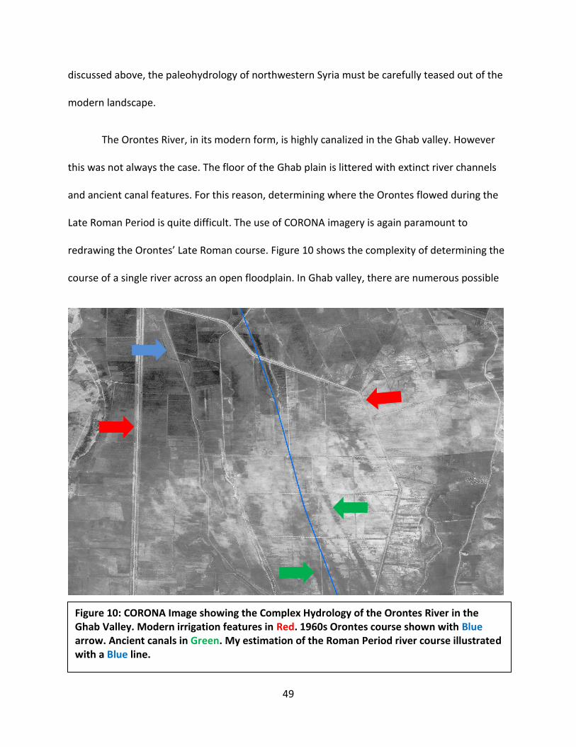
49

discussed above, the paleohydrology of northwestern Syria must be carefully teased out of the

modern landscape.

The Orontes River, in its modern form, is highly canalized in the Ghab valley. However

this was not always the case. The floor of the Ghab plain is littered with extinct river channels

and ancient canal features. For this reason, determining where the Orontes flowed during the

Late Roman Period is quite difficult. The use of CORONA imagery is again paramount to

redrawing the Orontes’ Late Roman course. Figure 10 shows the complexity of determining the

course of a single river across an open floodplain. In Ghab valley, there are numerous possible

Figure 10: CORONA Image showing the Complex Hydrology of the Orontes River in the Ghab Valley. Modern irrigation features in Red. 1960s Orontes course shown with Blue arrow. Ancient canals in Green. My estimation of the Roman Period river course illustrated with a Blue line.

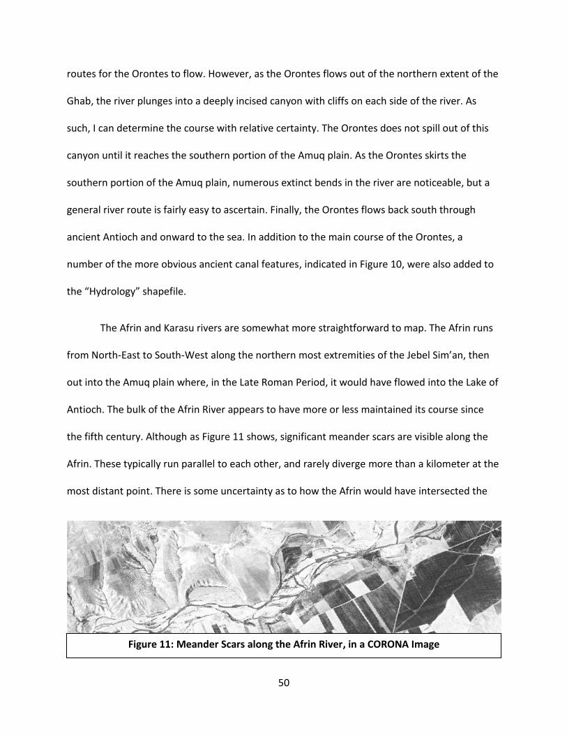
50

Figure 11: Meander Scars along the Afrin River, in a CORONA Image

routes for the Orontes to flow. However, as the Orontes flows out of the northern extent of the

Ghab, the river plunges into a deeply incised canyon with cliffs on each side of the river. As

such, I can determine the course with relative certainty. The Orontes does not spill out of this

canyon until it reaches the southern portion of the Amuq plain. As the Orontes skirts the

southern portion of the Amuq plain, numerous extinct bends in the river are noticeable, but a

general river route is fairly easy to ascertain. Finally, the Orontes flows back south through

ancient Antioch and onward to the sea. In addition to the main course of the Orontes, a

number of the more obvious ancient canal features, indicated in Figure 10, were also added to

the “Hydrology” shapefile.

The Afrin and Karasu rivers are somewhat more straightforward to map. The Afrin runs

from North-East to South-West along the northern most extremities of the Jebel Sim’an, then

out into the Amuq plain where, in the Late Roman Period, it would have flowed into the Lake of

Antioch. The bulk of the Afrin River appears to have more or less maintained its course since

the fifth century. Although as Figure 11 shows, significant meander scars are visible along the

Afrin. These typically run parallel to each other, and rarely diverge more than a kilometer at the

most distant point. There is some uncertainty as to how the Afrin would have intersected the

51

Lake of Antioch. The modern course is canalized as soon as it reaches the open Amuq plain, but

Wuelersse (1940) suggests that the Afrin would have flowed directly into an extension of the

Lake of Antioch north of the modern canal. Furthermore, in the CORONA imagery there is a

channel of the Afrin that runs north of the modern canal and intersects the Lake further to the

north. In light of this evidence, this was the final route chosen for the Afrin River.

The Karasu River runs north to South along the western edge of the Amuq plain. The

northern portions of the Karasu are straightforward to map, but as the Karasu reaches the

openness of the Amuq Plain proper, it becomes nearly invisible. Predictably the modern course

of the Karasu is highly canalized. CORONA images suggest a number of possible river channels.

Even Wuelersse’s usually detailed maps are somewhat lacking on the Karasu. Due to this dearth

of reliable information, an approximate river course was chosen between the end of the

obvious river course and the point at which the Karasu intersects the Lake of Antioch. Although

all of the suspected river courses are approximate, the southern portion is tenuous even by

comparison.

The importance of the Lake of Antioch is difficult to overstate. Libanius’ Oration in Praise

of Antioch is filled with admiration for the lakes and rivers surrounding Antioch.

“Is it then surprising that we, who inhabit such a country and enjoy such a trading place who

have as an ally the lake, and have the highway of the river as a helper, is it surprising that we

adorn the city as though for a festal assembly”? (Downey 1959: 680)

Clearly Libanius is fond of The Lake of Antioch. He goes as far as to cite it as an “ally” and gives

it considerable credit for the prosperity of Antioch (In Praise of Antioch 260-266). Libanius

speaks of the Lake as an economic and agricultural asset, not a hindrance. Although writing

52

more than a century before the peak of settlement along the limestone massif, it is reasonable

to assume that this positive attitude about the Lake likely continued into the fifth and sixth

centuries. However this attitude did not survive into the present. The draining of the Lake in the

mid-twentieth century caused severe ecological repercussions (Casana 2008). Despite its

permanent draining in the 1960s, evidence for the past extent of the Lake of Antioch is ample.

In the winter of 1970, the Lake still held a considerable amount of water. Even in modern

imagery, the footprint of the Lake is clearly evident by the stark difference in soil color. Figure 12

shows a comparison of the Lake of Antioch while it still held water, and how it appears in modern

imagery. Although these images show the Lake after efforts to drain it were already underway, they

provide a general outline of the extent of the Lake. Since the Lake was fed by both the Afrin and Karasu

Rivers, the actual volume of the Lake likely changed significantly with the seasons. As such, renderings

of the Lake of Antioch from these images very likely underestimate its original size.

The Marshes in the Amuq and Ghab basins are perhaps the most challenging feature of the

landscape to reconstruct. It is well known that in the early 20th century these marshes stretched over

Figure 12: The Lake of Antioch in CORONA mission 1112-2203Aft December 2nd 1970 (left) and in modern Google Earth Imagery (right)

53

large portions of both valleys (Eger 2011; Wieser 2012). However the formation of these marshes and

their salience in the Late Roman countryside is a matter of no small debate. Both Eger’s (2011) and

Weulersse’s (1940) estimate reflect twentieth century marsh extents. Evidence for the extent of these

marshes in the Late Roman Period is difficult to parse out. Libanius, in his glowing account of the

Antioch countryside, does not mention the words “marsh” or “swamp” once during his entire oration

(Downey 1959). Since Libanius fawningly describes practically every other aspect of the Antioch region,

this absence is striking. However, given the obvious bias Libanius has for the region, it is possible that he

simply omits a less pleasant feature of the landscape.

Modern archaeologists and geoarchaeologists are not in agreement over the areas these

marshes formed, nor even how they formed. Eger suggests that these marshes were, at least in part, the

result of much heavier precipitation between November and March (Eger 2000: 63). However, both Eger

(2000) and Casana (2008) feel that such widespread inundation (at least as was observed in the

twentieth century) of the Amuq and Ghab valleys probably did not take shape until after the Late Roman

Period. In fact, Casana (2008) sees the late period expansion of settlement into the surrounding

highlands as a primary driver for the erosion that would clog up the valleys and eventually re-inundate

the lowland valley floors. Some evidence, in the form of Roman canals visible in CORONA images,

suggests that although the marshes predate Roman influence, these marshes would have been drained

or at least much smaller by the fourth and fifth centuries (Casana 2008; Eger 2011; Wieser 2012). This is

firmly corroborated by the Amuq Valley Regional Project’s discovery of a number of Roman and Late

Roman sites on areas known to have been covered by the marshes (Casana and Wilkinson 2008). The

marshes appear to bookended Roman influence in the region. By the seventh century, as Roman

influence waned, the massive canals were no longer being maintained. It is reasonable that this neglect,

coupled with loose highland sediment, and periodic heavy rain, could overwhelm the Roman Period

canals and slowly inundate the valleys once more.

54

Despite this evidence to the contrary, it is worthwhile to incorporate the marshes into the Least

Cost Path model. Though it appears unlikely at this point, if present during the Late Roman period, these

marshes would have presented a considerable obstacle to regional trade and movement. Since

Weulersse and Eger map the marshes with slightly different extents, a simple Boolean intersection was

performed to establish an area of accord between Weulersse and Eger.

Topography

Given the broken and rough nature of much of the limestone massif, the influence of

topography on trade cannot be understated. To act as a stand-in for the physical topography, digital

elevation models (DEM) can be used. ASTER satellite imagery produces a DEM with a spatial resolution

of thirty meters.4 While resolution is not excessively high, especially compared to LiDAR data, it is the

highest resolution data freely available for northwestern Syria. In addition, this resolution is precise

enough to detect topographic and even some major cultural features, it is coarse enough to omit

modern features, such as highways and buildings, which would not have existed in the Late Roman

Period. The rugged massif itself is somewhat resistant to natural change. However, despite its

robustness, even the stone of the surrounding Jebels changes over time. These changes, such as

quarries and bulldozing, are unavoidable but relatively minor. From the ASTER DEM a slope model can

easily be created, which illustrates the changes in elevation from pixel to pixel. Once weighted properly,

the “Slope” becomes an approximation for the differential difficulty of moving across this rugged

landscape.

Settlements

The final component of the Late Roman landscape that must be considered is the presence and

location of Late Roman settlements. As discussed at length previously (Chapter Three), the exact

4 ASTER GDEM is a product of METI and NASA

55

locations of the Dead Cities were quite difficult to ascertain. While knowing the locations of the Dead

Cities is essential to test the viability of trade across this region as a whole, comparative sites are

needed.

Since the bulk of survey projects in and around the Ghab and Amuq valleys have primarily

focused on mounded “Tell” sites, Late Roman settlement patterns have traditionally been

underrepresented (Braidwood 1937; Courtois 1937; Marfoe 1979). Until fairly recently, only Tchalenko

(1953) has devoted significant attention to Roman and Late Roman sites. Fortunately, two University of

Chicago projects helped to correct this imbalance in the 1990s and mid-2000s.

The Amuq Valley Regional Project (AVRP) was one of the first archaeological projects to adopt

the use of CORONA imagery (Casana 2003; Casana and Wilkinson 2005). The AVRP documented a large

number of previously unknown late period sites. A shapefile containing all of the Roman and Late

Roman site locations was generously given to me by Jesse Casana. This shapefile contains 228 sites

covering the bulk of the Amuq Plain.

The Northern Ghab Regional Project helped to further elucidate the settlement history for the

Ghab Plain. This survey discovered sites ranging from Pre-Pottery Neolithic all the way forward to the

present (Graff 2006). Like the AVRP, the NGRS documented a considerable number of Late Roman sites.

This shapefile contains an additional sixty-six Late Roman sites in the Ghab valley. These sites were also

given to me by Jesse Casana.

Together, with the site location data from my remote sensing survey, these two survey

shapefiles help to reconstruct the settlement pattern of Late Roman Syria. Far from de Vogue’s notion of

the Dead Cities existing in an isolated landscape, we can now easily see that the Late Roman countryside

was densely occupied. Though these datasets are not exhaustive, they are a large enough sample size to

allow us to better understand both settlement patterns, and potential avenues of trade.

56

Conclusions

All landscapes are dynamic and complex, and this landscape is no exception. This chapter has

articulated one of many possible readings of the Late Roman landscape of northwestern Syria. Though

each of the facets discussed above is based on a variety of corroborating data, there are undoubtedly

inaccuracies and mistakes contained in these datasets. However, the true utility of digital approaches to

archaeology is their ability to be updated as new data emerges. As new data is published, or reevaluated

using new technologies, these datasets can easily be adapted to fit new paradigms and answer new

research questions. As such, perfection is not sought with this interpretation of the ancient landscape.

This data characterizes an approximation of a long past landscape, but one that has the capacity to be as

dynamic as the landscapes themselves. Figure 13 shows the full extent of the physical and cultural

landscape discussed in this chapter.

57

Figure 13: The Author’s reconstruction of the Late Roman Landscape

58

Chapter Five: Least Cost Path Model Construction

GIS model building is one of the most powerful avenues of investigation available to

archaeologists. These models offer the flexibility critical to properly examine cultural questions,

but are still robust in producing testable scientific data. The GIS platform ArcMap is used

throughout the model building process.

Chapter four detailed the types of data selected for representation in this model. This

chapter will discuss the incorporation and classification of this data into this model. If weighted

properly, this wide variety of physical and cultural data can be seamlessly shaped into a robust

model. Although a wide variety of GIS modelling techniques are available to researchers, this

specific type of modelling is referred to as Least Cost Path (LCP) analysis (White and Surface-

Evans 2012). Working within the framework set by the author, the GIS program will utilize

Raster data to compute the least costly pathway between points. On a perfectly flat isotropic

plain, the shortest distance would, of course, be a straight line. However, as this model is

constructed, differential values or “weights” will be given to each type of data. These data will

be scaled to attempt to replicate the actual experience of moving across a physical landscape.

For example, moving up a steep slope is noticeably more difficult than walking along a flat

plain. As the slope increases, the weight given to the data will also increase. Each dataset is

given a specific weight based broadly on trial and error. Once all of the data is combined into a

single continuous raster surface, the resulting “pathways” function as a potential avenue of

movement across the landscape. Each pathway is given a unique number and therefore can be

59

compared against each other. From these resulting pathways we can begin to examine the

differences in difficulty and duration of trade and travel from each village to the urban areas.

One more consideration before the model is constructed: since the aim of this model is

to test the viability of olive oil trade from Dead Cities, this model will be constructed with the

assumption of overland trade. This overland trade would likely have used carts or wagons

transporting heavy amphorae, or caravans of donkeys and camels hauling skins fill with oil

(Decker 2009). This assumption is somewhat flawed from the outset. Libanius specifically states

that the Orontes was a major avenue of trade (Libanius XI: 260-265). In fact, Libanius paints a

picture of the Lake and rivers as funneling trade goods right into the heart of Antioch, and later

out to the Mediterranean Sea (Libanius XI: 263-264). This presents a substantial challenge to

this model. Although the idea of the Orontes as an avenue of trade is fairly well attested, little is

known about the scale of trade along these routes, cost relative to land transport, or even what

types of cargos would be typically carried (Downey 1961; Libanius XI; Casana 2003).

Unfortunately this matter is further complicated by the nature of LCP analysis. LCPs are

excellent at treating a linear feature, such as a river, as either an impediment or an avenue.

However with LCPs there is not straightforward way of treating the river as both an impeding

and channeling force. This type of complexity is possible to model, but not without the creation

of a transport network from scratch. Furthermore, the utility of the Orontes as an avenue of

trade is accepted, but little else about river based trade is understood. For instance, there is

virtually no evidence regarding the scale or duration of river trade. It is also unclear which

individual actors would be involved in river trade. Was this an elite trade activity, or a means of

transport open to all traders? Without firm answers to these questions, the presence of river

60

based trade cannot be properly incorporated into the model. With these issues in mind, this

analysis assumes only overland trade.

Considering the Construction of the Model

The process of constructing a LCP model is inherently subjective. The relative value

given to each type of data heavily influences how the GIS produces the pathways. If the data is

weighted inconsistently or illogically, then the resulting pathways will be of little value.

Constructing the model is a negotiation of sorts. If the researcher, subconsciously or otherwise,

produces the model with specific expectations in mind, then the resulting data is compromised.

If the researcher does not scale the data properly across all facets, then one particular dataset

can be overrepresented in the model, thus heavily coloring the interpretation of the data. This

folly was noticeable in earlier iterations of this model. The Slope layer was not properly scaled

down, and the resulting model was dominated almost exclusively by the Slope values, to the

detriment of the other datasets.

With these serious considerations in mind, though still subjective, much thought has

been dedicated to the weighted value of each dataset. Given the number of sites and

complexity of this model, fairly small values are preferred to large ones. In general, data values

are assigned on a 1-10 scale. This ensures that the resulting data are express in manageably

small sums.

Rasterized Data

Raster GIS data are expressed through a series of rows and columns. These rows and

columns create numerous square units referred to as cells. This model will be constructed

61

primarily using raster GIS data. Each cell will be given values used to represent the accumulated

exertion of crossing each cell. The bulk of the data used to reconstruct the Late Roman

landscape was drawn in the form of vector GIS data. The data discussed in previous chapters

was primarily vector data. Vector data are expressed using points, lines, polylines, and

polygons. For this model to be functional, most of the vector data must be converted into a

raster format. Only the settlement shapefiles are able to remain vector data without disruption

of the process. This is because the point shapefiles act as the origin and destinations of the

pathways and are therefore not given a weighted value. In the interest of standardizing pixel

size, I opted to use the base resolution of the ASTER DEM to act as the uniform size. Although

ASTER DEM data has a world average of 30 meters resolution, the coverage of Syria is

approximately 25 meters. It is also important to note that all vector data layers were created

with an attribute column called “value.” The value column is where relative cost weights will be

applied later in the model building process. Value will also be the common attribute column

that links all base data together in a single continuous raster layer. Once all of the base data is

converted into raster format, then relative values can begin to be assigned to each layer.

Creation of Slope Layer

The creation of the Slope layer is straightforward. The tool Slope in ArcMap quickly

creates a slope layer from any DEM available. Using this tool, the ASTER DEM can easily be

converted into a Slope layer. The GIS does this by looking at the relative height of neighboring

pixels and calculating the degree of slope or the percent rise between pixels. The percent rise

option was used for this project. Since the slope layer is produced directly from the ASTER DEM

there is no need to specify a pixel size.

62

Reclassification of Data

This step is the heart of the model. Reclassification allows the researcher to specify

exactly what value should be given to each range of data. For example, slope data is often

displayed as a continuous “stretched” layer with unusably high data values. The Reclassify tool

breaks this stretched data into ranges that can be given more manageable data values, in this

case 1-10. This method of reclassification also mitigates outlier values that were abnormally

high or low, to produce a more representative approximation of the topography. The logic here

is simple: as the slope increases, so does the difficulty of crossing the landscape.

It is important to note that while reclassifying data, two additional considerations must

be made. Firstly, the extent of each layer must be identical. This will ensure that all data layers

are the same size. Next it is crucial that while reclassifying, the “NoData” pixels be given a value

of “0.” This will allow the GIS to composite all of the base layers together without distorting the

underlying data values of each layer. This effectively creates a binary between pixels with data

values and pixels without data values (NoData).

Unlike the Slope layer, the remainder of the base datasets do not need to be scaled

down. However each dataset must be individually weighted. The hydrology layer is fairly

straightforward. Though the Orontes River is larger than the Karasu or Afrin, I have chosen not

to assign them differing values. As such, all three rivers, plus the canal features included earlier,

will be given a very high value of 10. The reasoning behind assigning such a high value revolves

around the difficultly of transporting carts or caravans across wide rivers. It is reasonable to

assume that crossing a major river would be roughly equivalent to crossing the steepest terrain

63

found in the slope layer. With this high value, rivers will be treated as significant barriers. The

only exception to this high value would be the points at which the roads cross the river. During

the Late Roman Period these points of the river would have been traversed by bridges. Most of

these bridges crumbled long ago, but one is standing near the ancient Roman city of Cyrrhus,

near to northern extent of this survey region.

A special “Bridges” shapefile could have been generated for this project, but the manner

in which the Roman Road is incorporated into the model renders such an addition unnecessary.

The Roman Road must be built into the model in a way that would make them an attractive

route for the pathways. If a road is nearby it will be the easiest, least steep path, even if it not

the most direct route. Given the rough and broken terrain of the limestone massif, these well-

built Roman Roads, by comparison, would be paradise. Weighting the road values correctly is a

difficult task. I want the roads to be an attractive option for travel, but not so attractive as to

dominate the other data facets. As such, the roads layer was given a weighted value of “5.” This

might seem an odd choice at first, but the roads layer will be subtracted from, instead of added

to, the composite layer later on. In other words, all of the other data layers will be added into a

single composite layer, and then the roads layer will be subtracted from it. Effectively this will

render the area of the road a more cost effective option without creating a negative value.

Since negative values are both illogical and disrupt processing, they must be carefully avoided.

In essence, as the road crosses a river, the road will maintain its cost advantage over the

surrounding pixels. As such, no special “bridges” shapefile was needed.

64

Assigning value to the Lake of Antioch presents the same problem as the rivers. The

Lake was easily large enough to support both fishing and sailing, but it is impossible to discuss

the Lake’s role in regional trade at this point. As new data becomes available it might be

possible to reassess the Lake as a possible avenue of water based transport, but unfortunately

for now the Lake must be treated as an obstacle. Like the Hydrology layer, I opted to assign the

Lake of Antioch the highest value of “10.”

As discussed above, the marshes in both the Amuq and Ghab valleys present a challenge

to interpreting the Late Roman landscape. If present during the Late Roman Period, these

marshes would have been a substantial obstructing force to regional trade. These marshes

would have varied anywhere between soft boggy soil all the way up to standing fresh water,

possibly several feet deep. To cover this variability, a mid-range value of “5” was assigned to

the marshes. Since there are deep doubts over the presence and extent of the marshes during

the Late Roman Period, two iterations of the model will be created to address this issue. One

model with the marshes included, and one model without them. This will allow for a

comparison not only of the pathways themselves, but also the overall cost incurred.

Compositing the Base Layers into Friction and Cost Layers

Now that the base data layers are properly formatted, they can be combined into a

“friction” layer. This layer will be an amalgamation of all of the base data layers. The friction

layer will act as a composite stand-in for the accumulated difficulty of moving across each pixel.

The process of combining these layers is fairly straightforward. The tool Raster Calculator in

65

ArcMap allows the researcher to create a simple string of arithmetic that instructs the program

on how the researcher wishes the data to be compiled.

The data can be combined and recombined ad nauseam. The key to this step is to

combine the data in a way that is both meaningful and robust. Since I wish to test the model

first with the marshes present, and then without the marshes, I will need to make two separate

friction files. The Figure 14 contains the sum of all of the base layers, minus the Roman Roads,

plus the additional value of 6. This additional value is added for two specific reasons. First it

ensures that every pixel will have a data value. For example if there is a location on this model

that is flat and not covered by a river or marsh, then the base value would be “0.” However,

Figure 14: Friction Layer with Marshes Indicated

66

once the roads layer is subtracted, if it crossed over this pixel with a “0” value then it would

produce a value of “-5.” The program cannot understand negative values so this must be

avoided at all costs. In short, by adding “6” to each pixel I ensure that the lowest possible data

value per pixel is 1. The arithmetic string used to create the first friction layer (with marshes,

Figure 14) is as follows, with the resulting layer displayed below it.

"lake_antioch" + "hydrology" + "slope" + "marshes" + 6 - "roads"

This friction layer clearly illustrates both the Lake of Antioch and the marshes as having higher

values than most of the surrounding landscape. The Figure 15 is created using a very similar

arithmetic string. The only difference for this layer will be the exclusion of the marshes layer.

"slope" + "lake_antioch" + "hydrology" + 6 - "roads"

The resulting layer will appear very similar to the friction layer previously generated, but will

lack any of the information associated with the marshes. Both of these friction layers can now

act as an approximation of the environmental resistance incurred while traveling across a

landscape.

67

Now that the base data layers are all conveniently housed in one file, estimations of the cost of

travel can now begin to be made. There are several tools available to perform this calculation, but the

most effective is Cost Distance. This tool allows the researcher to choose a point or points of origin and

calculate the accumulation of cost outward. Figure 16 uses the Roman cities of Antioch and Apamea as

the points of origin for this process. Cost Distance not only creates a “cost” raster, but also creates a

“backlink” raster that contains directional movement data critical to generating pathways. Since the

“Cost” layer takes into account both physical and cultural data considerations, it can be read as a stand-

in for area of influence, or even extent of political control. With this step complete we can begin to

speculate on the potential areas of influence that each city might have commanded. Figure 16 suggests

that the northern cluster of the Dead Cities appear to mostly fall into the Antioch catchment area, while

the southern cluster of the Dead Cities appears to be much more closely related to Apamea.

Figure 15: Friction Layer Without the Marshes Included

68

Interestingly, there are a number of Dead City sites situated across the southern portions of the

Jebels Wastani Il A’la and Barisha that straddle the line between the two cities’ spheres of influence. In

rough terms of cost, these Dead Cities appear to be midway between either urban center. In addition,

we can now better appreciate the confining nature of the topography of the limestone massif.

Traversing either the Amuq or the Ghab valleys incurs little cost from the nearest city, but traveling even

a few kilometers up into the Jebel regions rapidly experiences higher cost. As might be expected, the

steep Jebels act as a funneling and confining force on travel from the cities. On an isotropic plane these

cost would increase outward in large graceful circles. By contrast the Cost layer shows hemming effects

of the topography, but also the extending power of the road systems. From each city, the low cost areas

extend furthest along the roads. This demonstrates the ability of well-maintained roads to extend

influence, even across rugged terrain.

Figure 16: Cost Layer Originating from Antioch and Apamea

69

Finally all of the data is in place to calculate the pathways themselves. These pathways will

illustrate the least costly path between each Dead City and the most accessible urban area. The tool Cost

Path will calculate the pathways. The process will take into account not only the “Cost” layer, but also

the “Direction” layer created above. Using these two raster layers simultaneously allows the program to

calculate the most efficient pathway from pixel to pixel. Figure 17 illustrates the results as a series of

direct pathways cascading down from the Jebels onto the fertile plains, and finally into the regional

urban centers.

Figure 17: Least cost Pathways between the Dead Cities and Urban Centers

70

Although these pathways are only hypothetical, they are able to provide a good estimate as to

how trade would have flowed across the landscape, particularly since transport of goods likely included

wheeled carts or caravans of animals. Not only do these pathways provide paths of least cost, they also

calculate cost in arbitrary units labelled as “PATHCOST.” These arbitrary units can easily be converted

into more meaningful units such as travel duration or energetics (kilocalories required). Most critically

for this project, the PATHCOST values can be directly compared across settlement datasets. In essence I

can compare the exertion required to travel from the Dead Cities directly against that required traveling

from the other Late Roman settlements. This head to head comparison can hint at the level of increased

difficulty incurred while crossing the Jebels. In turn, these values will help evaluate the viability of trade

across this landscape.

Conclusions

The pathways are drawn to the roadways, as areas of lower cost, but not overpoweringly so.

The topography clearly has a funneling effect on the pathways, but overall does not appear to greatly

restrict travel across the region. Practically all of the northern cluster of sites are drawn toward Antioch.

This is hardly surprising. The flat Amuq plain and the presence of the road along its southern edge

provide an excellent route for most of these sites. However, as Figure 18 shows, along the southern

portion of the Jebels Wastani and Barisha two sites are drawn southward toward Apamea. This two sites

hint at some fascinating findings. Firstly, these two sites are drawn into Apamea’s area of influence

despite a much greater Euclidean distance. From the first of these sites, Antioch is 35 kilometers away

while Apamea is 62 kilometers away, nearly double the distance. This implies that position and

ruggedness of the Jebels can have a very powerful effect on how travelers might have chosen move

across the landscape. This isn’t particularly surprising given the steepness and extent of the Jebels.

However, these two sites hint that the margins between the costs of going to either city might be much

finer than previously assumed. In fact, sites located just over a kilometer away from the sites in

71

questions are drawn to Antioch. The difference of a mere kilometer can have radical effect on the

resulting pathway. Such fine margins could well mean that despite this model’s findings, sites located in

this area of the Jebel Wastani and Jebel Il A’la are, in terms of cost accumulated, practically equidistant

to either city. This hints at a less obvious relationship between the Dead Cities and the urban centers.

Figure 18: Pathways Displayed Over the DEM with the Area Discussed In Red

µ

72

While these findings are encouraging, they must first be compared against other settlements of this

period before more firm statements about the viability of trade can be made.

Other Observations from the Models

In addition, possible areas of influence can be approximated using this approach. As

briefly discussed above, the Cost layer can be read as an area of possible influence. Given the

goals of this thesis, it is instructive to examine and compare the Cost layers generated for the

Roman Cities and the Dead Cities. The area of easy access around Antioch and Apamea is

logical. The flat Amuq and Ghab valleys are easily accessible, while the steeper Jebels are more

difficult to access. It is also notable how the roads carry influence further from each urban

center. The area of easy access (displayed in red) can be traced with a polygon. This allows the

suggested area of influence to be mapped quantitatively. Figure 19 provides a direct

comparison between these two Cost layers. Although fairly large, the proportion of the region

easily accessible to Antioch and Apamea is dwarfed by that accessible from the Dead Cities.

Admittedly, the Dead Cities are numerically superior and spread across a wider area, but

Figure 19: Comparison of the Roman Cities Cost Layer (Left) and the Dead Cities Cost Layer

(Right)

73

nevertheless the area that is easily accessible is substantially greater. Based on these Cost

layers, it is reasonable to infer that combined, Antioch and Apamea had easy access to

approximately 30,250 square kilometers. This is a massive territorial catchment. In fact, it is

approximately two and a half times higher than the 12,000 square kilometers that Decker

estimates for the combined hinterland of Antioch and Apamea (Decker 2009: 172). More

strikingly, the area of easy access of the Dead Cities is higher still. At 37,665 square kilometers,

the Dead Cities can easily access a massive swath of the surrounding landscape. This is fairly

logical. Traveling from the lowland urban centers to the Dead Cities would be made more

difficult by the steep Jebels. However, travelling from the Dead Cities, the terrain would

become more manageable as one moved down the Jebels and away from the Dead Cities.

While it is not a perfect stand-in for political control, these layers demonstrate a landscape that

is much more inter-accessible than one might have previously expected. Only 10 of the

currently mapped Dead Cities (8%) fall outside of Antioch and Apamea’s suspected area of

influence. Both Antioch and Apamea and 99% of the Late Roman valley settlements fall into the

Dead Cities area of access. In addition, this Dead Cities-centric area of access covers a wide

swath of territory to the north and east of the limestone massif, suggesting not only easy access

to Antioch, Apamea, and the coast, but also to the other principle cities of the region: Cyrrhus,

Chalcis, and Beoria. As Figure 20 shows, despite administratively belonging to Antioch or

Apamea, the Dead Cities occupy a zone that was bordered by the territory of practically every

major urban center in western Syria. This implies that instead of the hinterland barrier that it

has traditionally been viewed as, perhaps the limestone massif and its settlements can be

viewed as more a territorial bridge between the hinterlands of five different urban centers.

74

Figure 20: Cost Layer Generated from All Late Roman Urban Centers

75

Chapter Six: Olive Oil Case Study

Given the high value of olive oil, and the insatiable demand that Late Roman society

would have needed, mass exportation of olive oil could easily have led to the construction of

such obviously prosperous sites as the Dead Cities.

The Olive Oil Trade

The potential scale of trade between the Dead Cities and the wider eastern

Mediterranean is difficult to quantify. Decker creates an agriculture potential model that can

serve as useful approximation of output (Decker 2009: 169-173). It should be prefaced that I do

not entirely agree with Decker’s model. It appears likely that Decker overstates the number of

presses in the hinterland of Apamea and Antioch and therefore distorts the oil output. Despite

some misgivings, Decker’s model can serve as a possible “best case scenario.” For the sake of

internal consistency I will use the figures that Decker cites. Though not intended to be

specifically accurate, this model does give some sense of the massive scale of olive oil that

could be produced. Decker places the potential number of presses in the combined hinterlands

of Apamea and Antioch at between 9,000 and 10,000 (Decker 2009). Since this number includes

possible presses in the Amuq and Ghab valley’s this is almost certainly overstated. The figure of

3,850 presses across the limestone massif is more reasonable (based on 5.5 presses per village)

(Decker 2009). Based on replication of the pressing technology, it is estimated that each press

instillation could press between 4,000 and 8,000 liters of oil per pressing season. This is a

representation of only the smaller scale presses. Some of the larger presses could have

produced substantially more oil. Assuming that all of the 3,850 presses were active all at once,

76

we arrive at between 15.4 million and 30.8 million liters of oil produced annually. This is quite

possibly conservative given the number of presses and increased size of many of them. It is

worth estimating here how much oil would have been necessary to support the region.

Mattingly suggests that 20 liters of oil per year per capita is a fair rule of thumb, though some

have placed this number up to 50 liters (Mattingly 1988). Tate estimated the population of the

limestone massif at 300,000, while Decker estimates the population of Antioch and Apamea at

150,000 and 115,000 respectively (Tate 1992; Decker 2009: 20). To this we could add another

100,000 possible inhabitants of the valley settlements. This would put the overall population at

665,000. The estimated population of northwestern Syria would have required approximately

13.3 million liters of oil per year to subsist. This leaves us with a potential oil surplus

somewhere between 2.1 million and 17.5 million liters per year. While none of these numbers

were intended to be concrete, they do convey a sense of scale. Mattingly also cautions that

olive trees tend to produce a bumper harvest one year then substantially less the next year

(Mattingly 1988). As such, this massive surplus could not be guaranteed every year. However in

years of good harvest, this massive surplus represented a huge agricultural windfall.

It appears that the limestone massif alone was possibly able to meet all of the oil needs

of the region with plenty of surplus remaining. It is tempting to regard such a surplus as a

stockpiling for periods of poor production, however oil can only be stored for about a year

before it runs the risk of going rancid (Mattingly 1988). This clearly suggests that this surplus

was produced with the intention of trade. Given that the needs of the regional populous are

already met, it stands to reason that this surplus would be exported to other parts of the Late

Roman world. This oil was likely shipped in the LR1 amphorae. This amphorae type was

77

produced relatively locally, on the coasts of Cyprus and Celicia (southern coast of modern

Turkey), but LR1 sherds are found all over the eastern Mediterranean (Karagiorgou 2004;

Decker 2009). Wickham notes that these sherds are rarely found in the Dead Cities themselves

(Wickham2005). Rather than contradicting export trading, this observation quite possibly

reinforces it. Despite the roads, maneuvering a cart, loaded with heavy amphorae, up and

down the Jebels would have been slow, difficult and inefficient. Decker’s assertion that the oil

was brought down the Jebels in skins carried by donkeys or camels is possibly closer to the

mark (Decker 2009). The logistical concerns of oil shipment, and the massive scale of oil

potentially produced, suggest that the oil likely changed hands several time from press to table.

Tchalenko notes several “meeting houses” in a number of sites near the edges of the

limestone massif (Tchalenko 1953). Although this classification was critiqued by later

researchers, Tchalenko could quite possibly be correct. The high level of internal variation of

the Dead Cities sites definitely leaves room for individual site specialization. Perhaps some Dead

Cities specialized on the mass transport of oil, while other focused on its production? Given the

density and proximity of settlement this is hardly impossible, but given the paucity of

archaeological excavation in the sites, such a possibility remains only conjecture.

As it now appears likely that overland transportation was not prohibitively expensive,

and assuming Decker’s production model is at least semi-accurate, the possible markets for this

massive oil surplus extend in every direction. The major population centers of Chalcis, Beoria,

and Cyrrhus are likely destinations. The presence of a large military force in Syria cannot be

dismissed as a likely recipient of at least some oil (Pollard 2000). More distant eastern

78

population centers along the Euphrates River likewise cannot be ruled out as recipients. Many

of these suppositions are only theoretical at this point but, using this methodology, could be

more thoroughly explored.

However, most of the current evidence (some textual, but mostly ceramic) points to the

feeding of the oil into a wider eastern Mediterranean economy. Mattingly compares oil

production and export of Spain, Tunisia, and Tripolitania (Mattingly 1988). Mattingly concedes

that especially in the case of Spain, some oil was being shipped directly to Rome itself. The

exact circumstance of such activity, either government subsidies or individual economic

activity, is still up for debate. Nevertheless some form of seaborne trade was taking place

during the Roman period. Therefore, it stands to reason that, in one form or another,

transportation of bulk oil across the Mediterranean was probable during the Late Roman

Period. A general picture of the destinations of these oil shipments can be gleaned from the

recovery of LR1 amphorae. Karagiorgou estimates that in the early and mid-sixth century LR1

amphorae type made up as much as 10% of the ceramic deposit at Carthage, and more

impressively, 15% of the ceramics assemblage from Constantinople (Karagiorgou 2004; Decker

2001). The total ceramic assemblage of Constantinople for this period likely numbers in the

tens of millions. 15% of such a massive accumulation indicates a strong trade relationship. Such

massive cities are obvious destinations for oil shipments. Constantinople alone had a

population of at least 500,000 and therefore would need at least 10 million liters of olive oil per

year.

79

Even Decker’s optimistic estimations of Syrian olive oil productions come nowhere close to

supplying all the oil needed for the Late Roman Mediterranean population. It is likely more

accurate to view the limestone massif as only one of a number of major oil producing centers

across the Mediterranean basin. Tripolitania, Cyprus, Tunisia, and Spain all sported robust oil

exporting potential. However by the mid-fifth century, as the Dead Cities were hitting their

peak, Spain and Tunisia were lost to the empire. As such, it is probable that the burden of oil

production shifted eastward. In light of this increased burden, the volume of oil produced in the

Dead Cities and its place in greater interregional trade can be better understood.

80

Chapter Seven: Conclusions

Until now, the Dead Cities have been treated as an isolated phenomenon. This thesis

was designed not only to view the Dead Cities in the context of the Late Roman landscape, but

also to view these sites as only one portion of a densely populated region. The exact nature of

the olive oil trade in the Dead Cities has been much debated, but until now little quantifiable or

testable data has been presented.

Settlement Density

Even before the final models were completed, a number of interesting insights became

apparent. Most obviously, but woefully lacking in earlier literature, are the settlement patterns

of northwestern Syria. Late Roman settlement has traditionally been viewed as densely

populated, but confined to the limestone massif. However thanks to the work of the AVRP and

the NGRS, the Dead Cities can be viewed within the context of contemporaneous settlement.

Although none of these data sources are comprehensive, their combination gives us a partial

glimpse into the settlement density of the Late Roman period. As noted in chapter three, only

Dead Cities’ sites that could be verified with satellite imagery were included in this analysis. As

such, the limestone massif is less densely populated in Figure 21 than it would have been in

during the Late Roman period. The same is also true of the southern Ghab valley and Jebel

Nusayrism, neither of which has yet been fully surveyed.

81

While Figure 21 only reflects a portion of the likely settlement for this era, it does help

to visualize the Dead Cities as part of a densely populated region. Interestingly, the area of

highest density is in the south-western portion of the Amuq valley and the central area of the

Ghab valley, far from the heights of the Jebels. Despite their absence from literature discussing

the Dead Cities, based on current information, the lowland settlements actually possess a

higher settlement density.

Figure 21: Settlement Density in Late Roman Syria

0 50 10025

Kilometersµ

82

Discussion of the Models

The true power of GIS modelling is in its adaptive ability. Virtually any variable can be

added or removed from the model. If one source of data has become overrepresented, it is a

simple process to reevaluate its salience.

In an attempt to mitigate potential biases in any one model, five distinct models are

constructed. Each model is designed to illuminate particular questions, but can nevertheless

serve as interesting comparisons to each other. As briefly discussed in chapter four, the

presence and extent of the marshes in the Ghab and Amuq valleys are difficult to determine.

With this model-based approach, both scenarios can easily be examined. In addition to these

two models, one model with substantially higher data values was constructed (Higher

Resistance Model). In the two previously mentioned models, the rugged landscape of the

limestone massif did not appear to greatly affect the course of the pathways. To insure that this

was not an artifact of the values assigned to the slope data, I created this model with greatly

increased slope values for comparison.

The fourth model was designed to determine the potential effect of the small “inland

routes” evident in many of Tchalenko’s maps (Tchalenko 1953). These routes leave virtually no

traces and were therefore considered too subjective to be included in the earlier models.

However their potential to alter the calculation of pathways was too powerful to completely

dismiss. Finally, the elevation model doubled the initial values given to the slope layer, and

removed the Roman roads from consideration.

83

For the ease of comparison, the most relevant data was compiled into Table 1. Though

some of the calculated pathways changed somewhat from model to model, the resulting data

shows a remarkable consistency. This is most evident in the relationship between the average

Pathcost of the Dead Cities and the other Late Roman settlements. The Pathcost for each route

is calculated by dividing the total accumulated sum by the number of cells in each line. As such,

the average Pathcost can act as a stand-in for relative exertion required to travel along each

path. As Table 1 demonstrates, the average Pathcost accrued when traveling from the Dead

Cities was markedly higher, approximately double, than that accumulated traveling from the

valley settlements. This is not surprising. The valley settlements are located on the broad flat

plains, while the Dead Cities straddle the rugged limestone massif. In addition, the Dead Cities

are generally located further from either Antioch or Apamea. In fact, this distance and the

ruggedness of the Jebels were thought to represent the most logical barrier to trade.

0

1

2

3

4

5

6

7

8

MarshesIncluded

MarshesExcluded

HigherResistence

Inland RoutesIncluded

Elevation Model

Table 1: Average Pixel Cost Across Five Models

Late Roman Sites

Dead Cities

84

This logical assumption appears to be seriously overstated. Regardless of the

parameters used, each model produced a similar relationship between the average Pathcosts of

these sites. Simply put, each model determined that, on average, it requires approximately 1.75

times more exertion to reach the Dead Cities than it does to reach the valley settlements.

Admittedly, this exertion ratio does vary, but only slightly. This is especially striking

considering that each of these models was built intentionally to advantage or disadvantage

certain aspects of the landscape. As discussed above, the extensive marshes in the Ghab and

Amuq valleys would greatly hamper travel to and from the settlements therein. As such, this

model was built to accrue greater cost traveling across the open valley floors. This would clearly

advantage the Dead Cities, since they reside on the dry heights of the Jebels, far above the

marshes. Interestingly, though the valley settlement’s average did rise, the increase was

minimal.

Next the “inland routes” model adds additional low cost pathways crisscrossing the

Jebels themselves. These pathways function as miniature roads, allowing for lower cost travel

across the rough terrain. This model also incorporates the marshes in the valleys. Essentially

this model was the optimal combination of factors for travel through the Dead Cities. However,

as with all previous models, the exertion ratio hovered around 1.75 times more difficult.

Lastly, the elevation model doubled the slope values and removed the Roman roads

layer. This was designed to be a worst case scenario travel for the Dead Cities. With much

higher slope values and no channeling roads, the Dead Cities would seem to be isolated on the

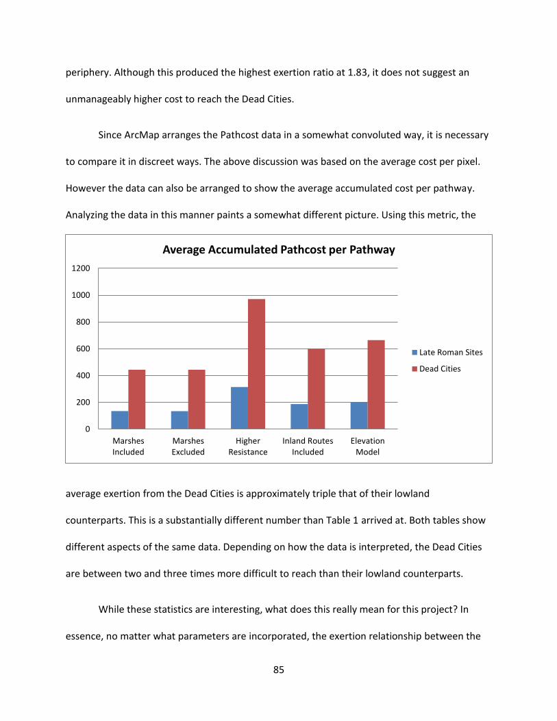
85

periphery. Although this produced the highest exertion ratio at 1.83, it does not suggest an

unmanageably higher cost to reach the Dead Cities.

Since ArcMap arranges the Pathcost data in a somewhat convoluted way, it is necessary

to compare it in discreet ways. The above discussion was based on the average cost per pixel.

However the data can also be arranged to show the average accumulated cost per pathway.

Analyzing the data in this manner paints a somewhat different picture. Using this metric, the

average exertion from the Dead Cities is approximately triple that of their lowland

counterparts. This is a substantially different number than Table 1 arrived at. Both tables show

different aspects of the same data. Depending on how the data is interpreted, the Dead Cities

are between two and three times more difficult to reach than their lowland counterparts.

While these statistics are interesting, what does this really mean for this project? In

essence, no matter what parameters are incorporated, the exertion relationship between the

0

200

400

600

800

1000

1200

MarshesIncluded

MarshesExcluded

HigherResistance

Inland RoutesIncluded

ElevationModel

Average Accumulated Pathcost per Pathway

Late Roman Sites

Dead Cities

86

valley settlements and the Dead Cities remain strikingly similar. If this ratio is not greatly

affected by changes made to the models then what is the driver of such a relationship? It

appears likely that the main source of this disparity of exertion lies not in topography or

hydrology, but in geography. Speaking in general terms, the valley settlements are located

much closer to the urban centers of Antioch and Apamea. The Dead Cities, on the limestone

massif, are generally located further from these urban centers. Since all of the iterations of the

models seem to imply that the landscape doesn’t play as significant a role as previously

assumed, it seemed likely that Euclidean distance could be the main driver of accumulated

exertion. Table 3 illustrates the relationship between the Euclidean distance of the Dead Cities

and valley settlements. Unsurprisingly, the relationship between the average Euclidean

distances (Dead Cities average divided by Valley settlements) equals 1.83. This closely parallels

Table 3: Average Euclidean DistanceSettlement Type Average Euclidean Distance

(to the nearest urban

center)

Exertion Ration

Late Roman Valley

Settlements

26.16 km

1.83 Dead Cities 47.97

the average pixel cost ratios discussed in Table 1. This implies that the main driver of increased

cost accumulation is distance. While the environmental and social factors (e.g. roads, slope, and

hydrology) do play a role in cost accumulation, it is relatively minor compared to the role

played by distance. While distance does not account for all of the difference of exertion, based

on the consistency of the above data, it seems to be the most salient aspect of overall

accumulated cost.

87

Using Casson’s suggested daily travel of 24-32 kilometers per day, on foot, these

distances can begin to be put into better context (Casson 1994: 188). Tracing the calculated

pathways between some of the farthest sites provides a rough estimate of travel time.

Following the calculated route, the most remote valley settlement is 82.41 kilometers from

Antioch. This is roughly between 2.5 and 3.5 days of travel time. The most remote Dead Cities is

139.08 kilometers away from Antioch. To reach this settlement, it would take between 4.3 and

5.7 days of travel. While these travel times are considerable, they are paltry compared to many

distances covered during the Roman and Late Roman periods (Casson 1994). Casson states that

during the Roman period, Imperial messengers would travel as many as 40 days to reach

Antioch from Rome (Casson 1994: 188). While this example is drawn from the Roman

administration, not the economy, it does demonstrate that destinations six days away should

not be viewed as especially far.

Although more travel time is required from the most remote of the Dead Cities than

many of the valley settlements, there are also a considerable number of the Dead Cities that

are roughly equivalent in terms of travel time. The presence of the good quality road between

Antioch and Chalcis seems to be a major factor. Overall, despite their distance to the cities, the

Dead Cities are more well-integrated within the road system. Only 1% of Dead Cities’ sites are

located more than 24 kilometers (one day’s travel time) from a road. 12% of the valley

settlements fall outside of one day’s travel to the nearest road. Admittedly these sites are in

the extreme northern Amuq plain, but as such, travel from these settlements would have to

traverse the Lake and possibly even the marshes. Furthermore the differential speed of road

travel versus off-road travel is a factor that would likely strongly assert itself.

88

In summary, across all of the models constructed there is a demonstrably higher

average cost of travel to and from the Dead Cities versus contemporary valley settlements.

Though considerable, this additional required exertion is not prohibitively high. This is

especially true when considering the high value and demand of olive oil.

In aid of the goals of this project, using these Cost layers as a guide, it is possible to

calculate the region of viable interaction. As the areas of access for both the Dead Cities and

the urban centers have already been calculated, it is a simple matter to perform a Boolean

calculation. Using the “Boolean And” tool, the GIS will automatically create a polygon of the

territory covered by both previous Cost layers. The resulting layer represents the areas that are

easy to access from both the Dead Cities and the urban centers of Antioch and Apamea (Figure

22). Since the estimation of the prices of ancient commodities is notoriously difficult, I am

Figure 22: Area of Mutual Low Cost Access and Exchange

0 50 10025

Kilometers

µ

89

hesitant to evaluate a region of viability of olive oil production based on bulk value and shipping

costs. In lieu of speculating on the value of commodities, this proposed sphere of interaction is

the best estimate of an area of viable trade interaction. All areas covered by the white polygon

are mutually low cost to access. Though potentially lasting for days or even a week at a time,

travel cost within this polygon is relatively low. Given the large number of the Dead Cities that

fall within this region, trade within this region appears not only viable, but potentially

extensive.

Economic Implications

This thesis strongly suggests that overland transportation, long thought to be far too

ponderous and inefficient, is in fact perfectly viable for this region. Furthermore, the Roman

roads skirting the perimeters of the Jebels integrated the Dead Cities into a regional system of

commerce and logistics practically invisible in the modern landscape. This case study has

produced a number of interesting insights into the local economic activity of Late Roman Syria.

However this information also has wider implications to the larger debate over the nature of

the ancient economies.

At first glance the widespread commodities trade and implied driving forces of supply

and demand appear to firmly support the “modernists” reading of ancient economies. However

it would be a mistake to purely equate modern notions of economic activity directly to ancient

history. Though many of the elements of the Late Roman economy appear capitalistic, there are

also powerful overarching economic forces at play.

90

During the early Roman period, the central authority devised a redistributive system,

the Annona, of subsidized grain and oil. This system was designed to keep high population

areas, such as Rome herself, well supplied. Food shortages foster civic discontent, something all

emperors fear. This system was so widespread that early historians viewed individual economic

activity as only possible through utilizing the extra space in the ship’s hold around these

subsidized goods (Duncan-Jones 1974).

The Roman and Late Roman emperors themselves were not strangers to widespread

economic policies and actions. In A.D. 362, Julian’s setting of the grain prices in Antioch upset a

number of wealthy grain merchants. Additionally in the reign of Anastasius, the emperor

forbade the export of olive oil to non-imperial territory in the northern Black Sea. These

examples demonstrate that the Emperors wielded the power to manipulate the economic

conditions based on their own needs and desires. Furthermore, each emperor would feasibly

have different economic ideas. Any emperor could expand or cancel the policies of their

predecessors. Furthermore the extensive system of taxes-in-kind to support large frontier

garrisons could have placed a massive burden on certain regions during the Late Roman period

(Pollard 2000). Since the volume and even types of goods collected are not well understood,

the potential effect on the economy is impossible to quantify. These potentially widespread

effects on the ancient economy are homogenized in modernist viewpoints. Though many of

these forces have modern capitalist equivalents, it appears that reading the Roman and Late

Roman economy as a direct analogue to modern capitalism is not entirely appropriate.

91

Though these findings appear to support modernist view of the ancient economy, it

does not completely dismiss elements of primitivist viewpoints. Tate and Sodini’s excavations

clearly demonstrated that local agriculture in the Dead Cities was, at least partially, geared

toward subsistence. Such local-centric subsistence could be construed as evidence for little

need of interregional interaction. However, as the next section will discuss in more detail, the

current evidence suggests that both widespread exportation for capital and small-scale

subsistence farming existed contemporaneously. This implies, at least in this case, neither of

the major interpretations of ancient economics fully captures the experience of the inhabitants

of the Dead Cities.

If anything, the findings of this thesis complicate the study of ancient economics.

Perhaps it is more apt to speak of a plurality of ancient economies. If these findings hold true

over the larger region, then it is more accurate to think of each settlement as engaged in

multiple economic behaviors simultaneously. The Dead Cities concurrently participated in at

least two wildly different economic models. Due to the coarse nature of the data on the Dead

Cities, it is unclear at present whether all of the Dead Cities engaged in both behaviors. It is

quite possible that individual sites, or even individual families, would have operated exclusively

in one economic sphere or another. The exact economic makeup of the Dead Cities is

impossible to determine with the current data. However, it does appear that the age-old

debate between modernists and primitivists does not fully articulate with experience of these

unique sites.

92

Abandonment

Like those that came before me, I cannot help but apply these new findings to the

abandonment of the Dead Cities. Tate and Sodini’s discovery of subsistence agriculture (fruits,

cereals, livestock, etc.) in the Dead Cities seemed to powerfully refute Tchalenko’s theories of

olive based monoculture. However, Tate and Sodini’s framing of olive production as a “cash

crop” does not fully explain the ubiquity of the presses across the limestone massif.

In light of the suggestions of this thesis, the limestone massif is better understood as a

dynamic and integral part of the northern Syrian political and economic landscape. The

prosperity of the Dead Cities was built upon and hedged by the olive oil trade, both

domestically and interregional. After the disastrous events of the sixth century, the Dead Cities

found themselves isolated from the greater Roman world, first temporarily, but following the

Arab conquest of Syria, permanently. Given the implication of increased viability of, and

suspected reliance on, trade markets for the oil, a relatively sudden alienation from these

markets would have been disastrous. While this would have represented as massive loss of

income capital, the subsistence needs of the population were still being met through local

agriculture (Tate 1992). The loss of the major source of capital explains how, though the Dead

Cities were occupied until the ninth century, building and rebuilding seems to have ceased by

about A.D. 550 (Foss 1996). Furthermore the disruption of the eastern Mediterranean trade can

be seen in the dearth of shipwrecks after A.D. 650 (Kingsley 2004). This is further corroborated

by the absence of any Umayyad pottery in the current shipwreck databases (Kingsley 2004: 35).

If Kingsley’s suggestion is correct, the limestone massif, now in Umayyad territory, would have

been cut off from the sea, and thus its most lucrative markets. These suggestions appear to

93

support Wickham’s theory of the local subsistence economy, supported by an interregional

“macroeconomy” based on oil (Wickham 2005). As it now appears, Tchalenko’s ideas of

regarding the abandonment of the Dead Cities may not have been as far from the mark as

previously thought. It is possible that Tchalenko had the driving forces of abandonment mostly

correct, but was incorrect in the rapidity of abandonment.

Conclusions

The findings of this thesis firmly suggest that trade and travel to and from the Dead

Cities was not only viable, but also, given the position of the limestone massif practically

assured. The density of population, both rural and urban, the extent of the roads, and the

obvious prosperity of the Dead Cities themselves already strongly suggests the presence of

intensive trade. This supposition is still more firmly supported by the findings of this thesis. All

iterations of the models support the relative viability of fairly long distance trade in this region.

Furthermore the extensive archaeological evidence for olive oil surplus in the Dead Cities

speaks to an oil producing economy that was clearly geared toward more than mere

subsistence. Mattingly (1988) suggests that olive oil cannot be stored for more than a year with

serious risk of the oil going rancid, thus stockpiling of oil can safely be ruled out the in the Dead

Cities. Finally and perhaps most critically, the recovery of LR1 amphorae regionally produced

and typically filled with oil or wine, all across the Mediterranean basin and beyond. In light of

this evidence, the reality that northwestern Syria was a major trade center, based at least

partially on the mass exportation of olive oil, becomes irrefutable. The Dead Cities, previously

viewed as isolated ruins, must now be understood as an critical component of the complicated

political, social, and economy fabric of Late Roman Syria.

94

References

ALCOCK, S.E. 1997. The Early Roman Empire in the East. Oxford, England: Oxbow Books.

BANG, P.F. 2007. Trade and Empire In Search of Organizing Concepts for the Roman Economy

Past & Present, 3–54.

BEATTIE, A. & T. PEPPER. 2001. The rough guide to Syria. 2nd ed. London: Rough Guides.

BRAIDWOOD, R.J. 1937. Mounds in the plain of Antioch, an archeological survey, Chicago, Ill.:

University of Chicago Press.

BRAIDWOOD, R.J. & L.S. BRAIDWOOD. 1960. Excavations in the Plain of Antioch. Chicago:

University of Chicago Press.

BRYCE, T. 2014. Ancient Syria . Oxford, England: Oxford University Press.

BURNS, R. 2009. The monuments of Syria a guide. Rev. London: I.B .Tauris.

BUTCHER, K. 2003. Roman Syria and the Near East. Los Angeles: J. Paul Getty Museum :

BUTLER, H.C. & F.A. NORRIS. 1930. Syria: publications of the Princeton University

archaeological expeditions to Syria in 1904-5 and 1909. Div. 1 Geography and itinerary.

Leyden: Brill.

BUTLER, H.C. & E.B. SMITH. 1929. Early churches in Syria, fourth to seventh centuries,

Princeton: Pub. for the Department of Art and Archaeology of Princeton University.

CALLOT, O. 1984. Huileries antiques de Syrie du Nord. Paris: Libr. orientaliste P. Geuthner.

CAMERON, A. 1998. The Cambridge ancient history. Cambridge: Cambridge University Press.

CASANA, J. 2004. The Archaeological Landscape of Late Roman Antioch, in Culture and Society

in Later Roman Antioch.

CASANA, J. 2007. Structural Transformations in Settlement Systems of the Northern Levant AJA

American Journal of Archaeology, 195–221.

CASANA, J. 2008. Mediterranean valleys revisited: Linking soil erosion, land use and climate

variability in the Northern Levant Geomorphology, 429–42.

CASANA, J., J. COTHREN. & T. KALAYCI. 2012. Swords into Ploughshares: Archaeological

Applications of CORONA Satellite Imagery in the Near East IA Internet Archaeology.

CASANA, J. & T. WILKINSON. 2006. Settlement and Landscapes in the Amuq Region. Essay, in

The Amuq Valley Regional Projects , 1: 25–66. Chicago, IL: University of Chicago.

95

CASANA, J. & M. PANAHIPOUR. 2014. Satellite-Based Monitoring of Looting and Damage to

Archaeological Sites in Syria Journal of Eastern Mediterranean Archaeology & Heritage

Studies, 128–51.

CASANA, J. 2014. The Late Roman Landscape of the Northern Levant: A view from Tell Qarqur

and the lower Orontes River Valley Oxford Journal of Archaeology , 193–219.

CASSON, L. 1994. Travel in the ancient world. Johns Hopkins Paperbacks. Baltimore: Johns

Hopkins University Press.

COURTOIS, J.-C. 1973. Prospection archéologique dans la moyenne vallée de l'Oronte (El-Ghab

et Er Roudj. Syrie du Nord-Ouest) Syria syria, 53–99.

CZAJLIK, Z. 2013. Aerial archaeology and remote sensing from The Baltic to The Adriatic:

selected papers of The Annual conference of The aerial archaeology research group, 13th-15th

September 2012, Budapest, Hungary. Budapest: Institute of archaeological sciences, Faculty of

humanities, Eotvos Lorand University.

DE JONG, M., F. THEUWS. & C. VAN RHIJN. (ed.) 2001. Topographies of Power in the Early

Middle Ages.

DE VOGUE, le C.M.de. 1865-77. Syrie centrale. Paris: Baudry.

DECKER, M. 2001. Food for an Empire: Wine and Oil Production in North Syria, in Economy

and exchange in the East Mediterranean during Late Antiquity: proceedings of a conference at

Somerville College, Oxford.

DECKER, M. 2001. Economy and exchange in the East Mediterranean during Late Antiquity:

proceedings of a conference at Somerville College, Oxford, 29th May, 1999. Oxford: Oxbow.

DECKER, M. 2009. Tilling the hateful earth: agricultural production and trade in the late antique

East. Oxford: Oxford University Press.

DENTZER, J.-M. & W. ORTHMANN. (ed.) 1989. Archeologie et Histoire de la Syrie II: La Syrie de

l'epoque achemenie a l'avenement de l'Islam.

DOWNEY, G. 1961. A history of Antioch in Syria: from Seleucus to the Arab conquest. Princeton,

N.J.: Princeton University Press.

DUNCAN-JONES, R. & K.R. BRADLEY. The Economy of the Roman Empire The American

Journal of Philology, 224–24.

EGER, A. 2008. The Spaces Between the Teeth: Environment, Settlement, and Interaction on the

Islamic-Byzantine Frontier, (Dissertation, University of Chicago) 1–612.

96

EGER, A.A. 2011. The Swamps of Home: Marsh Formation and Settlement in the Early

Medieval Near East* Journal of Near Eastern Studies 70: 55–79.

FINLEY, M.I. 1973. The ancient economy, Berkeley: University of California Press.

FOSS, C. 1996. Dead Cities of the Syrian Hill Country Archaeological Institute of America 49:

48–53.

FOSS, C. 1997. Syria in Transition, A. D. 550-750: An Archaeological Approach Dumbarton

Oaks Papers, 189–89.

FRANK, T. & A.C. JOHNSON. 1933. An economic survey of ancient Rome, Baltimore: The Johns

Hopkins Press.

FRANKEL, R. 1999. Wine and oil production in antiquity in Israel and other Mediterranean

countries. Sheffield: Sheffield Academic Press.

Google Earth Add photos 2015 - Earth Help. Accessed.

https://support.google.com/earth/answer/148126?hl=en.

GRAFF, S.R. 2006. Economy and society: an archaeological reconstruction of the political and

informal economy of northwestern Syria in the third millennium BC.

GREENE, K. 1986. The archaeology of the Roman economy. Berkeley: University of California

Press.

HARRIS, W.V. 1993. The inscribed economy: production and distribution in the Roman empire

in the light of instrumentum domesticum : the proceedings of a conference held at the American

Academy in Rome on 10-11 January, 1992. Ann Arbor, MI: University of Michigan.

HAYWOOD, R.M. & F.M. HEICHELHEIM. 1938. An economic survey of Ancient Rome, Baltimore:

The J. Hopkins Press.

Hirst K. Kris Biography - About's Guide to Archaeology 2015 About.com Education. Accessed.

http://archaeology.about.com/bio/k-kris-hirst-3021.htm.

HULL, D. 2008. A Spatial and Morphological Analysis of Monastic Sites in the Northern

Limestone massif, Syria Levant 40: 89–113.

JAKOBY, E. 2013. Considering Kranzhugeln: An Exploration into the Structural Variation and

Environmental/Spatial Distribution of the Thrid Millennium "Kranzhugel" Sites, (Master’s

Thesis, University of Arkansas) 1–123.

JONG, L.D. 2007. Narratives of Roman Syria: A Historiography of Syria as a Province of Rome

SSRN Electronic Journal SSRN Journal.

97

KARAGIORGOU, O. 2009. Mapping trade by the Amphora, in Mapping trade by shipwrecks , in

Byzantine trade, 4th-12th centuries: the archaeology of local, regional and international

exchange : papers of the thirty-eighth Spring Symposium of Byzantine Studies, St John's College.

KARAKHANIAN, A., V. TRIFONOV., T. IVANOVA., A. AVAGYAN., M. RUKIEH., H. MININI., A.

DODONOV. & D. BACHMANOV. 2008. Seismic deformation in the St. Simeon Monasteries (Qal'at

Sim'an), Northwestern Syria Tectonophysics, 122–47.

KAROLL, A. 2011. The Early Bronze Age IV to Middle Bronze Age I Transition in the Orontes

Valley, Syria: A View From Tell Qarqur. (Master’s Thesis, University of Arkansas)

KINGSLEY, S. 2009. Mapping trade by shipwrecks, in Byzantine trade, 4th-12th centuries: the

archaeology of local, regional and international exchange : papers of the thirty-eighth Spring

Symposium of Byzantine Studies, St John's College.

LIBANIUS. 1959. Libanius' oration in praise of Antioch (oration XI). Philadelphia, Pa.: American

Philosophical Society.

MANGO, M.M. 2000. The Commercial Map of Constantinople Dumbarton Oaks Papers 54: 189–

89.

MANGO, M.M. 2009. Byzantine trade, 4th-12th centuries: the archaeology of local, regional and

international exchange : papers of the thirty-eighth Spring Symposium of Byzantine Studies, St

John's College, University of Oxford, March 2004. Farnham, Surrey, England: Ashgate Pub.

MANGO, M. 2009. Byzantine trade: Local, regional, interregional and International , in Byzantine

trade, 4th-12th centuries: the archaeology of local, regional and international exchange : papers

of the thirty-eighth Spring Symposium of Byzantine Studies, St John's College.

MARX, K. & F. ENGELS. 1967. Capital; a critique of political economy. New York: International

Publishers.

MATTINGLY, D.J. & J. SALMON. 2001. Economies beyond agriculture in the classical world.

London: Routledge.

MATTINGLY, D. 1987. Libyans and the 'limes' : culture and society in Roman Tripolitania antaf

Antiquités africaines, 71–94.

MATTINGLY, D.J. 1988. Megalithic Madness And Measurement. Or How Many Olives Could An

Olive Press Press? Oxford Journal of Archaeology Oxford J Archeol, 177–95.

MATTINGLY, D.J. 1988. Oil for export? A comparison of Libyan, Spanish and Tunisian olive oil

production in the Roman empire Journal of Roman Archaeology J. Roman archaeol., 33–56.

MATTINGLY, D.J. 1988. Olea Mediterranea Journal of Roman Archaeology, 153–61.

98

MLEKUŽ, D. 2014. Exploring the topography of movement Computational Approaches to the

Study of Movement in Archaeology Theory, Practice and Interpretation of Factors and Effects of

Long Term Landscape Formation and Transformation.

MOOG, S. 2015. Stand Strong, Stand Proud: Alternative and Pariah Femininities In San Diego's

Punk Rock Community (Master’s Thesis, University of Arkansas).

MOUTERDE, R. & J. LAUFFRAY. 1945. Le Limes de Chalcis. Organisation de la steppe en

Haute Syrie romaine. Documents aeriens et epigraphiques. Plans et releves de J. Lauffray et S.

Mazloum. (Texte.-Atlas.).

POIDEBARD, A. 1934. La trace de Rome dans le desert de Syrie; le limes de Trajan a la conquete

arabe; recherches aeriennes (1925-1932). Paris: P. Geuthner.

POLANYI, K. 1957. The great transformation. Boston: Beacon Press.

POLANYI, K. 1957. Trade and market in the early empires: economies in history and theory.

Glencoe, IL: Free Press.

POLANYI, K. & H.W. PEARSON. 1977. The livelihood of man. New York: Academic Press.

POLLARD, N. 2000. Soldiers, cities, and civilians in Roman Syria. Ann Arbor: University of

Michigan Press.

SAHLINS, M. 1972. Stone age economics. Chicago: Aldine-Atherton.

SANDWELL, I. & Huskinson, J. 2004. Culture and society in later Roman Antioch: papers from a

colloquium, London, 15th December 2001. Oxford: Oxbow Books ;

SARRIS, P. 2011. Empires of faith: the fall of Rome to the rise of Islam, 500-700. Oxford

[England: Oxford University Press.

SMITH, M.E. 2004. The Archaeology of Ancient State Economies Annu. Rev. Anthropol. Annual

Review of Anthropology, 73–102.

SODINI, J. & G. TATE. 1981. Dehes (Syrie du nord). Paris: Librairie orientaliste P. Geuthner.

TARLACH, G. How Google Earth Has Revolutionized Archaeology Discory Magazine.

TATE, G. 1992. Les Campagnes de la Syrie du Nord du IIe au VIIe siecle: un exemple

d'expansion demographique et economique a la fin de l'Antiquite. Paris: Librarie orientaliste

Paul Geuthner.

TATE, G. 1997. The Syrian Countryside during the Roman Era, in The Early Roman Empire in

the East. Oxford, England: Oxbow Books.

99

TCHALENKO, G. 1953. Villages antiques de la Syrie du Nord; le massif du Belus a l'epoque

romaine. Paris: P. Geuthner.

TCHALENKO, G. 1979. Eglises de village de la Syrie du nord. Paris: Librairie orientaliste P.

Geuthner.

TEMIN, P. 2001. A Market Economy in the Early Roman Empire The Journal of Roman Studies

91: 169–81.

UR, J.A. 2012. CORONA Satellite Imagery and Ancient Near Eastern Landscapes

SpringerBriefs in Archaeology Mapping Archaeological Landscapes from Space, 21–31.

VERHAGEN, P., S. POLLA. & I. FROMMER. 2014. Finding Byzantine junctions with Steiner trees

Computational Approaches to the Study of Movement in Archaeology Theory, Practice and

Interpretation of Factors and Effects of Long Term Landscape Formation and Transformation.

WARD-PERKINS, B. 1998. The Cities, in The Cambridge ancient history. Cambridge.

WEBER, M. & T. PARSONS. 1947. The theory of social and economic organization.

WEBER, M. 1958. The Protestant ethic and the spirit of capitalism. [Student's. New York:

Scribner.

WEST, L.C. 1924. Commercial Syria under the Roman Empire Transactions and Proceedings of

the American Philological Association , 159–59.

WEULERSSE, J. 1940. L'Oronte. Etude de fleuve. Par Jacques Weulersse.

WHITE, D.A. & S.B. BARBER. Geospatial modeling of pedestrian transportation networks: a case

study from precolumbian Oaxaca, Mexico Journal of Archaeological Science, 2684–96.

WHITE, D.A. & S. SURFACE-EVANS. 2012. Least cost analysis of social landscapes

archaeological case studies. Salt Lake City: University of Utah Press.

WICKHAM, C. 2005. Framing the early Middle Ages Europe and the Mediterranean 400-800.

Oxford: Oxford University Press.

WIESER, A. 2012. Geoarchaeology of the Orontes River Floodplain Surrounding Tell Qarqur,

Syria. (Master’s Thesis, University of Arkansas)

WILL, E. 1997. Antioche sur l'Oronte, métropole de l'Asie Syria syria, 99–113.

WILKINSON, T. 1999. Holocene Valley fills of Southern Turkey and Northwestern Syria: Recent

geoarchaeological contributions Quaternary Science Reviews, 555–71.

100

YENER, K.A., C. EDENS., T.P. HARRISON., J. VERSTRAETE. & T.J. WILKINSON. The Amuq Valley

Regional Project, 1995-1998 American Journal of Archaeology, 163–63.

YENER, K.A. 2005. The Amuq Valley regional projects. Chicago, IL: Oriental Institute of the

University of Chicago.

101

Appendix 1: Tchalenko’s Maps of the Dead Cities

102

103