Tractable Parameterizations for theMinimum Linear Arrangement Problem

Michael R. Fellows1, Danny Hermelin2,Frances Rosamond1, and Hadas Shachnai3

1 School of Engineering and IT, Charles Darwin University, Darwin, Australia.Email: {michael.fellows,frances.roasmond}@cdu.edu.au

2 Department of Industrial Engineering and Management, Ben-Gurion University,Beer-Sheva, Israel. Email: hermelin@bgu.ac.il

3 Computer Science Department, Technion, Haifa 32000, Israel.Email: hadas@cs.technion.ac.il

Abstract. The Minimum Linear Arrangement (MLA) problem asksto embed a given graph on the integer line so that the sum of the edgelengths of the embedded graph is minimized. Most layout problems areeither intractable, or not known to be tractable, parameterized by thetreewidth of the input graphs. We investigate MLA with respect to threeparameters that provide more structure than treewidth. In particular, wegive a factor (1+ε)-approximation algorithm for MLA parameterized by(ε, k), where k is the vertex cover number of the input graph. By a simi-lar approach, we describe two FPT algorithms that exactly solve MLAparameterized by, respectively, the max-leaf and clique-cover numbers ofthe input graph.

1 Introduction

Given a graph G = (V,E), a linear arrangement is a linear ordering on the set ofvertices V of G which is specified by a permutation π : V → {1, 2, . . . , |V |}. Thecost of the arrangement is defined by cost(π) =

∑(u,v)∈E |π(u)− π(v)|; that is,

the cost of the ordering is the sum total of the edge lengths under the ordering.In typical applications one is interested in linear arrangements of low cost. TheMinimum Linear Arrangement (MLA) problem is the problem of finding alinear arrangement of minimum cost, and the standard parameterization of theproblem is to determine if an input graph G has a layout of cost at most k (theparameter).

MLA is one of the most important and well studied graph ordering problems.It is in some sense closely related to the Bandwidth problem, which seeks tominimize the maximum edge length of an ordering of the vertices. It has variousapplications, most of which stem from the domain of VLSI circuit design. As itwas known to be NP-complete already from the mid 70’s [11], most of the earlywork on this problem focused on designing heuristics and approximation algo-rithms. For a graph with n vertices, the best known approximation ratio for MLAis O(

√log n log log n), due to Feige and Lee [5], and Charikar, Hajiaghayi, Karloff

and Rao [4]. Earlier notable work include the paper by Rao and Richa [17] whopresented an O(log n)-approximation algorithm for the problem, along with an-other algorithm for planar graphs that achieves a ratio of O(log log n). Recently,Ambuhl, Mastrolilli, and Svensson [1] showed that MLA does not admit a PTASunless NP-complete problems can be solved in randomized subexponential time.We refer the reader to [17] for a further account of earlier work on MLA.

In terms of parameterized complexity, the standard parameterization ofMLA is trivially fixed-parameter tractable (FPT). Gutin et al. presented in [13]an FPT algorithm which, given a graph on n vertices and m edges, and a pa-rameter k, outputs a linear arrangement of cost at most m + k, if one exists.Fernau in [10] described efficient bounded search tree FPT algorithms for MLAunder its standard parameterization. Bodlaender et al. [3] investigated exactexponential-time algorithms for several ordering problems, including MLA.

Most parameterized problems are FPT parameterized by the treewidth of theinput graph. However, graph layout and width problems are a notable exception(but see also [6] for further examples of parameterized problems that are W [1]-hard when parameterized by the input treewidth, or even the input vertex covernumber). Parameterized by the treewidth of the input graph, Bandwidth isknown to be hard for W [t] for all t (this follows from the results in [2]). Whethersomething similar holds for MLA is unknown. This general situation motivatesstudying the complexity of these problems, parameterized by structural parame-ters even stronger than treewidth, a program that is sometimes called parameterecology. See [7] for a recent survey of this area.

In this paper, we consider the complexity of MLA parameterized by threestructural parameters that have a certain commonality: all three, when bounded,force the input graph G to have a structure, that essentially consists of an elab-oration of some small (parametrically bounded) “seed” graph H, that gives ussufficient information about the entire graph G to be able to derive efficientalgorithms. The three graph structural parameters we consider are:

(i) The vertex cover number ofG, denoted vc(G), which is the size of the smallestset of vertices intersecting every edge in G.

(ii) The maximum leaf number of G, denoted m`(G), which is the maximumnumber of leaves in any spanning tree of G.

(iii) The edge clique cover number of G, denoted ecc(G), which is defined to bethe minimum number of clique required to cover all the edges of G.

The question of whether MLA is FPT by the vertex cover number of theinput graph has been prominently raised in [9], where it is shown that a numberof graph layout and width problems such as Bandwidth, Cutwidth and Dis-tortion are FPT by this parameter, and this question has been a noted openproblem in parameterized algorithmics. Here we offer a partial positive answerby taking an approach that combines parameterization and approximation. Oneof our main results shows that MLA can be approximated to within a factor of(1 + ε) of optimal, in FPT time for the aggregate parameter (1/ε, k), where k isthe vertex cover number of the input graph. (Whether the MLA problem can beexactly solved in FPT time for the parameter k alone still remains open.) In [8]

2

it is shown that Bandwidth is FPT, parameterized by the max leaf number ofthe input graph. Here we obtain a matching result for MLA; it can be exactlysolved in FPT time for this parameter. While the techniques used in both re-sults look similar from a bird’s eye, there are several major differences hiding inthe details. Finally, our last result shows that the edge clique cover number canpotentially be a useful parameterization for other graph layout problems.

The paper is organized as follows. In Section 2 we give a (1+ε)-approximationfor MLA parameterized by vc(G). In Sections 3 and 4 we present FPT algorithmsfor MLA using the parameters m`(G) and ecc(G), respectively. We conclude inSection 5 with some open problems. Due to space constraints some of the proofsare given in the Appendix.

2 MLA parameterized by Vertex-Cover Number

In this section we present an algorithm which yields a (1 + ε)-approximation forMLA in FPT-time with respect to k = vc(G) and 1/ε, where G is the inputgraph and ε > 0. Our algorithm proceeds as follows.

W.l.o.g., we assume that G has no isolated vertices, and let m = |E|. The firststep of our algorithm is to compute a vertex cover V ′ ⊆ V of G of size k. Notethat each vertex in V \ V ′ has neighbors only in V ′. We say that two verticesv1, v2 ∈ V \ V ′ are of the same type if N(v1) = N(v2), where N(u) denotesthe set of neighbors of a vertex u in G. Clearly there are T ≤ 2k differenttypes of vertices in V \ V ′. We let nt denote the number of vertices of type t,1 ≤ t ≤ T . The main idea of our algorithm is as follows. We put together verticesof the same type into groups of an appropriately chosen size, and then computean optimal linear arrangement for the graph obtained by merging each groupinto a single mega-vertex. The analysis of our algorithm relies on an interestinghomogeneity lemma which relates to the behavior of vertices of identical typeinside “gaps” formed by the vertices of V ′ in an optimal arrangement for G. Adetailed description of the algorithm is given below.

2.1 Analysis

We now prove that the algorithm yields a solution that is within factor (1 + ε)from the optimal.

Theorem 1. Algorithm 1 computes a (1 + ε)-approximate linear arrangementfor G in FPT time with respect to k and 1/ε.

We use in the proof of the theorem a few lemmas. Given a layout π for G,let u1, . . . , uk denote the vertices in V ′ as ordered in π. We say that a vertexv ∈ V \ V ′ is in gap i, 1 ≤ i ≤ k − 1, if π(ui) < π(v) < π(ui+1). Similarly, vis in gap 0 if π(v) < π(u1), and in gap k if π(uk) < π(v). The following lemmashows that the vertices of V ′ \ V appear homogenously according to their typein some optimal linear arrangement of G.

3

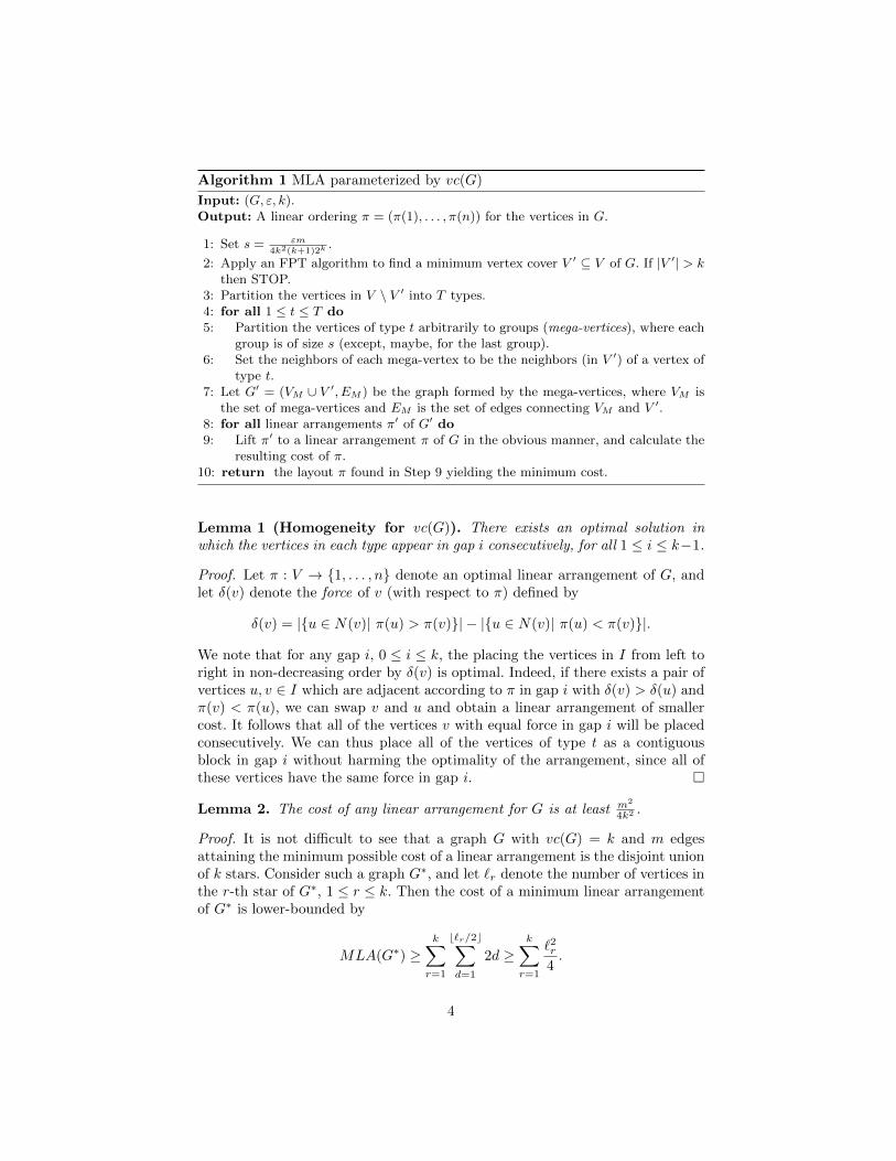
Algorithm 1 MLA parameterized by vc(G)

Input: (G, ε, k).Output: A linear ordering π = (π(1), . . . , π(n)) for the vertices in G.

1: Set s = εm4k2(k+1)2k

.

2: Apply an FPT algorithm to find a minimum vertex cover V ′ ⊆ V of G. If |V ′| > kthen STOP.

3: Partition the vertices in V \ V ′ into T types.4: for all 1 ≤ t ≤ T do5: Partition the vertices of type t arbitrarily to groups (mega-vertices), where each

group is of size s (except, maybe, for the last group).6: Set the neighbors of each mega-vertex to be the neighbors (in V ′) of a vertex of

type t.7: Let G′ = (VM ∪ V ′, EM ) be the graph formed by the mega-vertices, where VM is

the set of mega-vertices and EM is the set of edges connecting VM and V ′.8: for all linear arrangements π′ of G′ do9: Lift π′ to a linear arrangement π of G in the obvious manner, and calculate the

resulting cost of π.10: return the layout π found in Step 9 yielding the minimum cost.

Lemma 1 (Homogeneity for vc(G)). There exists an optimal solution inwhich the vertices in each type appear in gap i consecutively, for all 1 ≤ i ≤ k−1.

Proof. Let π : V → {1, . . . , n} denote an optimal linear arrangement of G, andlet δ(v) denote the force of v (with respect to π) defined by

δ(v) = |{u ∈ N(v)| π(u) > π(v)}| − |{u ∈ N(v)| π(u) < π(v)}|.

We note that for any gap i, 0 ≤ i ≤ k, the placing the vertices in I from left toright in non-decreasing order by δ(v) is optimal. Indeed, if there exists a pair ofvertices u, v ∈ I which are adjacent according to π in gap i with δ(v) > δ(u) andπ(v) < π(u), we can swap v and u and obtain a linear arrangement of smallercost. It follows that all of the vertices v with equal force in gap i will be placedconsecutively. We can thus place all of the vertices of type t as a contiguousblock in gap i without harming the optimality of the arrangement, since all ofthese vertices have the same force in gap i. �

Lemma 2. The cost of any linear arrangement for G is at least m2

4k2 .

Proof. It is not difficult to see that a graph G with vc(G) = k and m edgesattaining the minimum possible cost of a linear arrangement is the disjoint unionof k stars. Consider such a graph G∗, and let `r denote the number of vertices inthe r-th star of G∗, 1 ≤ r ≤ k. Then the cost of a minimum linear arrangementof G∗ is lower-bounded by

MLA(G∗) ≥k∑

r=1

b`r/2c∑d=1

2d ≥k∑

r=1

`2r4.

4

The function∑k

r=1`2

4 above is minimized when `r = mk for all 1 ≤ r ≤ k. Thus,

MLA(G∗) ≥ m2

4k2 , and the lemma follows. �

Lemma 3. Let MLA(G) denote the cost of the optimal arrangement for G,and let MLA(G′) denote the cost of the layout returned by Algorithm 1. Then

MLA(G′) ≤MLA(G) + εm2

4k2 .

Proof of Theorem 1: Observe that the running time of Algorithm 1 canroughly be bounded by the number of linear arrangements of G′. Note that|E′| = dm/se = O(2kk3) and |V ′| ≤ 2|E′|, as G′ has no isolated vertices. Thus,the total running time of the algorithm can be bounded by O∗((2kk3)!). Fur-thermore, by Lemmas 2 and 3, we have

MLA(G′)

MLA(G)≤ 1 +

εm2

4k2 ·MLA(G)= 1 + ε,

where MLA(G′) denotes the minimum cost of the layout returned by the al-gorithm, and MLA(G) denotes the optimal cost. Thus, Algorithm 1 returns a(1 + ε)-approximate solution in FPT time with respect to (ε, k). �

3 MLA parameterized by Max-Leaf Number

In this section we give an FPT algorithm for MLA parameterized by k = m`(G),for k > 1. We start with some definitions. Given a graph H = (V ′, E′), asubdivision of an edge e′ = (u, v) ∈ E′ replaces e′ by a path of length (ne′ + 2),for some ne′ ≥ 1, given by (u, v1, . . . , vne′ , v). Thus, the edge e′ becomes anedge-path, and we add to H ′ ne′ vertices. We say that a graph G is a subdivisionof a graph H if G was generated by subdivision operations on the edges of H.

As shown in [15], if m`(G) = k then G is a subdivision of a graph H on atmost 4k− 2 vertices. We call H = (V ′, E′) where V ′ ⊆ V and |V ′| = k′ ≤ 4k− 2the seed graph of G. Let S ⊆ E′ denote the set of subdivided edges in H. Then,V = V ′ ∪ (∪e′∈S{v1, . . . , vne′}), and E = E′ \ S ∪ {(z, w)| z ∈ V \ V ′, w ∈ V }.We say that a vertex w ∈ V \ V ′ belongs to e′, where e′ = (u, v) ∈ E′, if w is onthe path (u, v1, . . . vn′

e, v) in G.

Our algorithm for MLA, parameterized by m`(G), branches on an exhaustiveset of solution patterns which has size bounded by a function of k. This set ofpatterns contains at least one optimal solution for the graph G, if one exists.Then, to determine when a solution pattern can be realized, we solve a linearinteger program which outputs placements for all vertices of G in a permuta-tion that is consistent with the given pattern. A detailed description is given inAlgorithm 2.

We define a permutation π of the vertices in G, by extending a permutationσ of the vertices in H. Given such a permutation σ, we now formulate an integerlinear program to find the position of vertices in V \ V ′ among the vertices ofH. Recall that any permutation σ = (vj1 , . . . , vjk′ ) of V ′ defines (k′ + 1) gaps.Let π be a permutation of V that is consistent with σ. Let π(v) ∈ [n] denote the

5

Algorithm 2 MLA parametrized by m`(G)

Input: (G, k).Output: A linear ordering π = (π(1), . . . , π(n)) for the vertices in G.

1: Let H = (V ′, E′) be the seed graph of G, where E′ = {e1, . . . , em′}2: for all permutations σ ∈ Sk′ of the vertices in V ′ do3: for all configurations of E′, C = (Ce1 , . . . , Cem′ ) do4: Solve an integer linear program to determine the position of vertices in V \V ′

among vertices in V ′, such that the total cost is minimized (see details below).

5: return a permutation σ of V ′ which yields minimum cost for G.

position of vertex v ∈ V in π, where n = |V |. We say that a vertex w ∈ V \ V ′is placed in gap i in π , 1 ≤ i ≤ k′ − 1, if π(vji) < π(w) < π(vji+1), wherevji , vji+1

∈ V ′; w is placed in gap 0 (k′) if π(w) < π(vj1) (π(w) > π(vjk′ )).

A configuration for an edge-path of e′ ∈ E′ is a (k′ + 1)-vector, Ce′ =(ce′,0, . . . , ce′,k′), in which the i-th entry is equal to ’1’ if gap i contains a vertexin e′, and ’0’ otherwise. Let |E′| = m′. Then, a configuration for E′ is a set of m′

configuration vectors for all edge-paths in E′. We use in the integer program thevariables xe′,i to indicate the number of vertices on the edge-path of e′ ∈ E′ inthe i-th gap, 0 ≤ i ≤ k′. Let σ ∈ Sk′ be a permutation of the vertices in V ′. Wedenote by Cost(G|σ, x) the total cost of the linear arrangement of the verticesin G, with the given permutation σ and the variable values. This cost can becomputed in FPT time, using Lemma 4 (see Section 3.1). Then our program canbe formulated as follows.

(LPm`) : minimize Cost(G| σ, x)

subject to:

k′∑i=0

xe′,i = ne′ ∀ e′ ∈ E′

xe′,i = 0 if ce′,i = 0

xe′,i ∈ {1, . . . , ne′} if ce′,i = 1

3.1 Analysis

We now prove that Algorithm 2 yields an optimal solution. Our analysis cruciallyrelies on the next two lemmas.

6

Lemma 4 (Homogeneity for m`(G)). There exists an optimal layout inwhich vertices in V \ V ′ that belong to the same edge-path appear consecutivelyin gap i, for all 0 ≤ i ≤ k′.

Proof. Given a permutation π of the vertices in G, we show below that if theordering of vertices in gap i does not satisfy the contiguity property in thelemma then we can modify the order of vertices to satisfy the property, withoutincreasing the total cost. Given the permutation π, we say that a vertex v ∈ V \V ′is a right-bend of an edge-path if its two neighbors, u,w, satisfy π(u) < π(v) andπ(w) < π(v), i.e., both u and w appear to the left of v in π. Similarly, v is aleft-bend if its two neighbors appear to its right in π.

In proving the lemma, we distinguish between two cases:

(i) Gap i does not contain a vertex that is a bend of an edge-path; thus, for anyvertex v in gap i and its two neighbors, u,w, either π(u) < π(v) < π(w), orπ(w) < π(v) < π(u). Suppose that gap i contains two adjacent vertices z, v,that belong to different edge-paths, generated from e′1, e

′2 ∈ E′, respectively.

More precisely, let π = (vi1 , . . . , x, . . . , u, . . . v, z, . . . , w, . . . r, . . . , vin), wherer, x are the neighbors of z on the edge-path of e′1, and u,w are the neighborsof v on the edge-path of e′2. Let π be the permutation resulting from a swapof z and v in π, then the difference between the costs of the two permutationsis given by

cost(π′)− cost(π) = [(π(r)− π(z) + 1) + (π(w)− π(v)− 1)+(π(z)− π(x)− 1) + (π(v)− π(u) + 1)]−[(π(r)− π(z)) + (π(w)− π(v))+(π(z)− π(x)) + (π(v)− π(u))] = 0

Hence, we can perform a sequence of such swaps, until we have that all ofthe vertices that belong to the same edge-path appear consecutively in gapi, without increasing the cost.

(ii) Suppose that gap i contains a vertex v that belongs to an edge-path ofe′1 ∈ E′, where v is a bend. W.l.o.g. we assume that v is a right bend, i.e.,its two neighbors, u and w, appear to the left of v in π (the proof is similarfor the case where v is a left bend). Suppose that π(w) < π(u) < π(v),and assume that the vertex z /∈ e′1 precedes v in gap i, i.e., we have π =(vi1 , . . . , w . . . , u, . . . , z, v, . . . , vin). We show that swapping z and v does notincrease the total cost. Let π′ be the resulting permutation. We consider thefollowing cases:

(a) If z is not a bend, then it has two neighbors x, r, such that π(x) < π(z) <π(r). Hence, we have that cost(π′)− cost(π) < 0.

(b) Suppose that z is a right bend, then its two neighbors in theedge-path, x, r, are positioned to the left of z in π. W.l.o.g.,assume that π(x) < π(r) < π(z). More precisely, let π =(vi1 , . . . , x . . . , w, . . . , r, . . . , u, . . . z, v, . . . , vin). Then, it is easy to verifythat cost(π′)− cost(π) = 0.

7

(c) If z is a left bend then its two neighbors, x, r, are positioned toits right in π. W.l.o.g., assume that π(z) < π(r) < π(x), andπ = (vi1 , . . . , w . . . , u, . . . , z, v, . . . r, . . . , x, . . . , vin). Indeed, as a resultof the swap, both v and z become closer to their neighbors. Hence,cost(π′)− cost(π) < 0. �

Lemma 5. Given a permutation σ ∈ Sk′ for V ′, and the number of vertices ofedge-path e′ in gap i, xe′,i, 0 ≤ i ≤ k′, there exists an optimal order for V whereeach gap i for which xe′,i > 0 contains exactly one or two contiguous segmentsof e′.

Theorem 2. There is an FPT algorithm for MLA parameterized by the maxi-mum leaf number.

We use in the proof the next lemma.

Lemma 6. Given a permutation σ and the vector x, Cost(G| σ, x) is linear andcan be computed in FPT time.

Proof. We can write Cost(G| σ, x) =∑k′

i=0 Cost(gap i|σ, x), whereCost(gap i|σ, x) is the contribution of gap i to the total cost. Specifically, sup-pose that the two ends of gap i are x, y ∈ V ′, where π(x) < π(y). Let (v1, . . . , vh)be a segment of edge-path e′ in gap i. W.l.o.g., we assume that v1 is closer to x.Then we compute the contribution of this segment to the cost of gap i as follows.We compute the cost incurred by each internal edge on this segment and addto that a term that depends on the type of the segment. By Lemma 5, we mayassume that the segment (v1, . . . , vh) is contiguous.

(a) If the segment is straight (i.e., has no bend in gap i), we add the distancefrom v1 to x and from vh to y. This term would then partially account forthe cost incurred by the edges connecting the two ends of the segment, v1and vh, to their neighbors in other gaps.

(b) If the segment has a right bend, we add the distance between v1 and x plusthe distance between vh and x.

(c) If the segment has a left bend, we add the distance between v1 and y andthe distance between vh and y.

Thus, it suffices to show that Cost(gap i|σ, x) is linear and can be computed inFPT time. We now show how to order optimally the segments in gap i. Let B`, Br

and S denote the sets of segments of types left-bend, right-bend and straight in gapi, respectively. We denote by zi =

∑e′∈E′ xe′,i the number of vertices assigned

to gap i. We give the proofs of the next claims in the Appendix.

Claim 3 The cost incurred by any segment of type S in gap i is equal to zi.

Claim 4 Given a set of segments in Br in gap i, of lengths xe1,i ≤ xe2,i ≤ · · · ≤xer,i, the minimum total cost incurred by these segments in gap i is given byr · xe1,i + (r − 1)xe2,i + · · · + xer,i. Similarly, given a set of segments in B`, oflengths xe1,i ≤ xe2,i ≤ · · · ≤ xe`,i, the minimum cost incurred by these segmentsis ` · xe1,i + (`− 1)xe2,i + · · ·+ xe`,i.

8

Thus, letting |Br| = r and |B`| = `, by Claims 3 and 4 we have that the totalcost of gap i is given by

Cost(gap i|σ, x) = |S| ·∑e′∈E′

xe′,i +

r∑j=1

(r− j + 1)xej ,i +∑j=1

(`− j + 1)xej ,i, (1)

where e1, . . . , er are the edge-paths having in gap i segments in Br, and e1, . . . , e`are the edge-paths having in gap i segments in B`. For a vector x that is consis-tent with a given configuration of E′, we have that the values of r and ` in (1)are fixed, thus Cost(gap i|σ, x) is linear, and so is Cost(G|σ, x). Hence, we cansolve the integer program in FPT time (see, e.g., [16, 14]). �

Proof of Theorem 2: Clearly, by Lemmas 4 and 5, our algorithm exhaustivelysearches over the set of solution patterns which contains an optimal one. Itremains to show that the algorithm runs in FPT time. We note that the twoouter loops of Algorithm 2 require O(k′! · 2k2

) iterations, each requires solvingan integer linear program having O(k2) variables. This gives the statement ofthe theorem. �

4 MLA parameterized by Edge-Clique-Cover Number

In this section we show that MLA parameterized by the edge clique cover numberof a the graph is in FPT. More precisely, we prove the following theorem:

Theorem 5. There is an O∗(2k!)-time algorithm for MLA where k = eec(G) isthe edge clique cover number of the input graph G.

Two vertices u, v ∈ V of G are said to be of the same type if N [u] = {u} ∪N(u) = {v}∪N(v) = N [v], where N(u) and N(v) respectively denote the set ofneighbors of u and v in G. Note that our notion of type here is different from theone we use in Section 2, as vertices of the same type are necessarily adjacent.Nevertheless the two different concepts of types are conceptually very similar,as we can prove a certain homogenous lemma for this notion of type as well.

Lemma 7 (Homogeneity for ecc(G)). There exists an optimal vertex order-ing which is homogenous. That is, an ordering in which vertices of each typeappear consecutively.

Proof of Theorem 5 [assuming Lemma 7]: By Lemma 7, there exists anoptimal solution in which vertices of each type appear consecutively. Observethat in any such homogenous ordering, the ordering of vertices of the same typecan be arbitrary. That is, reordering vertices of a given type does not affect thetotal edge lengths of the ordering. Now, it is well known that a graph with edgeclique cover number at most k has at most 2k different types [12]. Thus, ouralgorithm searches through all O(2k!) homogenous vertex orderings and outputsthe best one. �

9

Algorithm 3 MLA parametrized by ecc(G)

Input: (G, k).Output: A linear ordering π for the vertices of G.

1: Compute the type of each vertex of G.2: Compute the cost of each homogenous ordering of types.3: return a homogenous ordering with minimum cost.

To prove Lemma 7, we introduce some additional notation. For an orderingπ = V → {1, . . . , n} and a pair of vertices u, v ∈ V such that π(u) < π(v), welet ←−−πu,v and −−→πu,v denote the following permutations:

←−−πu,v(x) =

π(x) if π(x) ≤ π(u) or π(v) < π(x),

π(u) + 1 if x = v,

π(x) + 1 if π(u) < π(x) < π(v),

and

−−→πu,v(x) =

π(x) if π(x) < π(u) or π(v) ≤ π(x),

π(v)− 1 if x = u,

π(x)− 1 if π(u) < π(x) < π(v).

Thus, ←−−πu,v is the vertex ordering obtained from π by placing v directly after u,and −−→πu,v is the ordering obtained from π by placing u directly before v.

Lemma 8. Let π = V → {1, . . . , n} be an optimal vertex ordering, and let uand v be two vertices of the same type with π(u) < π(v). Then both ←−−πu,v and−−→πu,v are optimal as well.

Proof. Define three set of vertices A = {x ∈ V : π(x) < π(u)}, B = {x ∈V : π(u) < x < π(v)}, and C = {x ∈ V : π(v) < π(x)}, and consider the

two quantities←−∆ = cost(←−−πu,v) − cost(π) and

−→∆ = cost(−−→πu,v) − cost(π). As π is

optimal, both these quantities are non-negative, i.e.←−∆ ≥ 0 and

−→∆ ≥ 0. If the

lemma were false, at least one of these quantities would be strictly positive, i.e.

we would either have←−∆ > 0 or

−→∆ > 0. Aiming towards a contradiction let us

assume that←−∆ > 0 (the proof in case

−→∆ > 0 is symmetric).

Let us examine which edges contribute to←−∆ , i.e. which edges {x, y} ∈ E

have different lengths in −−→πu,v and π (|−−→πu,v(x)−−−→πu,v(y)| 6= |π(x)−π(y)|). Clearly,

edges in E(A,A), E(B,B), E(C,C) and E(A,C) do note contribute to←−∆ . All

other edge lengths are different in the two orderings. The length of each edgein E(v, C) increases by |B| in ←−−πu,v when compared to its length in π, while thelength of each edge in E(v,A) decreases by |B|. Similarly, the length of each edgein E(A,B) increases by 1, while the length of each edge in E(B,C) decreasesby 1.

What remains to account for are the edges involving u and v. Let `(u,B) =∑b∈B |π(u)− π(b)| and `(v,B) =

∑b∈B |π(v)− π(b)| denote the total length of

10

the edges of E(u,B) and E(v,B) with respect to π. Observe that as u and v aretwins (and are thus adjacent to the same set of vertices in B), the total lengthof all edges of E(v,B) becomes `(u,B) in ←−−πu,v, while the length of each edge ofE(u,B) increases by 1. Thus, the total contribution of edges in E(u,B)∪E(v,B)

to←−∆ is |E(u,B)| + `(u,B) − `(v,B). Finally, the last edge contributing to

←−∆

is the edge {u, v} itself (which necessarily exists as u and v are from the sametype) whose length decreases by |B| in ←−−πu,v when compared to π.

Summing up all these contributions, we get the following equality for←−∆ :

←−∆ = |E(v, C)| · |B| + |E(A,B)| + `(u,B) + |E(u,B)|− |E(v,A)| · |B| − |E(B,C)| − `(v,B) − |B|. (2)

Symmetrically, a similar calculation will give us the following equation for−→∆ :

−→∆ = |E(u,A)| · |B| + |E(B,C)| + `(v,B) + |E(v,B)|− |E(u,C)| · |B| − |E(A,B)| − `(u,B) − |B|. (3)

Now as u and v are twins, we know that |E(u,A)| = |E(v,A)| and |E(u,C)| =|E(v, C)|. Furthermore, we also have |B| ≥ |E(u,B)| = |E(v,B). Thus, using

equations (2) and (3), and our assumption that←−∆ > 0 and

−→∆ ≥ 0, we get

|E(v, C)| · |B| + |E(A,B)| + `(u,B) + |E(u,B)| >|E(v,A)| · |B| + |E(B,C)| + `(v,B) + |B| ≥

|E(u,A)| · |B| + |E(B,C)| + `(v,B) + |E(v,B)| ≥|E(u,C)| · |B| + |E(A,B)| + `(u,B) + |B| ≥

|E(v, C)| · |B| + |E(A,B)| + `(u,B) + |E(u,B)|

our desired contradiction. �

Proof of Lemma 7: Let π be an optimal vertex ordering. If π is not homogenouswe can use Lemma 8 repeatedly to transform it into one. The lemma thus follows.

5 Summary and Open Problems

We have shed light on the complexity of MLA for structural parameterizationsstronger than treewidth, including a nice example of a successful combinationof parameterization and approximation. We believe our algorithmic strategy inthis may be widely applicable. Can this success be extended to the aggregateparameterization based on treewidth? In this paper we have aimed only at qual-itative FPT results. We leave the best running times for such FPT algorithmsas an open problem.

11

References

1. C. Ambuhl, M. Mastrolilli, and O. Svensson. Inapproximability results for max-imum edge biclique, minimum linear arrangement, and sparsest cut. SIAM J.Comput., 40(2):567–596, 2011.

2. H. L. Bodlaender, M. R. Fellows, and M. T. Hallett. Beyond NP-completenessfor problems of bounded width: hardness for the W hierarchy. In Proceedings ofthe 26th Annual Symposium on the Theory of Computing (STOC), pages 449–458,1994.

3. H. L. Bodlaender, F. V. Fomin, A. M. C. A. Koster, D. Kratsch, and D. M. Thilikos.A note on exact algorithms for vertex ordering problems on graphs. Theory ofComputing Systems, 50(3):420–432, 2012.

4. M. Charikar, M. T. Hajiaghayi, H. J. Karloff, and S. Rao. l22 spreading metricsfor vertex ordering problems. In SODA, pages 1018–1027, 2006.

5. U. Feige and J. R. Lee. An improved approximation ratio for the minimum lineararrangement problem. Inf. Process. Lett., 101(1):26–29, 2007.

6. M. R. Fellows, F. V. Fomin, D. Lokshtanov, F. A. Rosamond, S. Saurabh, S. Szei-der, and C. Thomassen. On the complexity of some colorful problems parameter-ized by treewidth. IInformation and Computation, 209(2):143–153, 2011.

7. M. R. Fellows, B. M. P. Jansen, and F. A. Rosamond. Towards fully multivariatealgorithmics: Parameter ecology and the deconstruction of computational complex-ity. European Journal of Combinatorics, 34(3):541–566, 2013.

8. M. R. Fellows, D. Lokshtanov, N. Misra, M. Mnich, F. A. Rosamond, andS. Saurabh. The complexity ecology of parameters: An illustration using boundedmax leaf number. Theory Comput. Syst., 45(4):822–848, 2009.

9. M. R. Fellows, D. Lokshtanov, N. Misra, F. A. Rosamond, and S. Saurabh. Graphlayout problems parameterized by vertex cover. In ISAAC, pages 294–305, 2008.

10. H. Fernau. Parameterized algorithmics for linear arrangement problems. DiscreteApplied Mathematics, 156(17):3166–3177, 2008.

11. M. R. Garey and D. S. Johnson. Computers and intractability: a guide to the theoryof NP-completeness. W. H. Freeman, 1979.

12. J. Gramm, J. Guo, F. Huffner, and R. Niedermeier. Data reduction and exactalgorithms for clique cover. ACM Journal of Experimental Algorithmics, 13, 2008.

13. G. Gutin, A. Rafiey, S. Szeider, and A. Yeo. The linear arrangement problemparameterized above guaranteed value. Theory Comput. Syst., 41(3):521–538, 2007.

14. R. Kannan. Minkowski’s convex body theorem and integer programming. Mathe-matics of Operations Research, 12:415–440, 1987.

15. D. J. Kleitman and D. B. West. Spanning trees with many leaves. SIAM J. DiscreteMath., 4(1):99–106, 1991.

16. H. Lenstra. Integer programming with a fixed number of variables. Mathematicsof Operations Research, 8:538–548, 1983.

17. S. Rao and A. W. Richa. New approximation techniques for some linear orderingproblems. SIAM J. Comput., 34(2):388–404, 2004.

12

A Some Proofs

Proof of Lemma 3: Consider an arbitrary optimal arrangement π for G.We note that in Step 9 of the algorithm we consider only assignments withan integral number of mega-vertices of each type in the gaps. However, itmay be the case that π contains fractional assignments of mega-vertices insome gap. Nevertheless, the increase of the number of vertices in any of thegaps in the corresponding integral assignment is at most s · 2k = ε′m

4k2(k+1) .

Thus, Algorithm 1 considers an assignment where the length of each edge in-creases by at most εm

4k2 in comparison to its length in π, and the lemma follows. �

Proof of Lemma 5: Suppose that the edge-path of e′ contains the vertices(a, v1, . . . , vh, b), where a, b ∈ V ′ and v1, . . . , vh ∈ V \V ′. Thus, e′ incurs cost forh + 1 edges. For any edge on this path, the cost of connecting two neighboringvertices vi, vj that appear in different gaps is 2 or higher, since at least one vertexin V ′ separates between these vertices in the vertex ordering, π, .there is anoptimal ordering for V which assigns we in each gap either a single contiguoussegment, or two contiguous segments of e′. Let σ(a) = f and σ(b) = g, andassume w.l.o.g. that 1 ≤ f < g ≤ k′. Let L = min{i | xe′,i > 0}, and L =max{i | xe′,i > 0}, i.e., L and R are the indices of the leftmost and rightmostgaps that contain vertices of e′, respectively. We first consider the cost incurredby internal edges, i.e., edges connecting neighboring vertices of e′ that are placedin the same gap.

W.l.o.g., we may assume that xe′,i > 1 We distinuish between the followingcases.

1. R ≥ g and L ≤ f − 1 (see Figure 1). Then we consider four types of gaps.

(i) In any gap f ≤ i ≤ g − 1, e′ must contain a vertex z ∈ {v1, . . . , vh}having neighbor in gap j ≥ i + 1, and a vertex x ∈ {v1, . . . , vh} havingneighbor in gap j′ ≤ i− 1, by the vector xie′ . We can take a contiguoussegment of length t = xe′,i, given by (vs, . . . , vs+t−1), and assign thesevertices consecutively from left to right, i.e., π(vi) = π(vi−1) + 1, for alls+ 1 ≤ i ≤ s+ t− 1. Thus, the cost incurred by each internal edge is 1.

(ii) In gap R, e′ must contain at least two vertices which have neighborsin gaps to the left of R. As argued above, if an edge between two ver-tices in e′ is external (i.e., its ends are placed in different gaps), the costincurred by this edge is at least 2. Let xe′,R = q, and consider a con-tiguous segment (xp, . . . , xp+q−1). Let d = bq/2c. We choose vp+d as aright-bend and order the vertices of the segment from left to right as fol-lows: (vp, vp+q−1, vp+1, vp+q−2, . . . , vp+d−1, vp+d+1, vp+d). Then, the costincurred by each internal edge in this segment is at most 2.

(iii) Similarly, we can order the vertices of a contiguous segment in gap Lwith a single left-bend, such that each internal edge incurs at most thecost 2.

(iv) If R > g, or L < f − 1, then there exist some gap i in which two verticesof e′ must have neighbors in gaps to the right of i, and two vertices must

13

Fig. 1. The layout of an edge-path connecting a and b: Case 1. in the proof of Lemma5

have neighbors to the left of i (see the vertices x, u and y, w in Figure1). In each such gap, we can assign two contiguous segments of e′ andorder each as a straight line. The cost incurred by each internal edge inthese segments is 1.

2. R ≥ g and L > f−1. Similar to Case 1., except that there is no left-bend(see Figure 2).

3. R < g and L ≤ f − 1. Similar to Case 1., except that there is no right-bend.

4. R < g and L > f − 1. In this case, the edge-path of e′ has neither aright-bend nor a left-bend. Therefore, we are in sub-case (i) of 1.

Fig. 2. Case 2. in the proof of Lemma 5

14

Hence, we may assume that any gap i for which xe′,i > 0 contains eitherone or two contiguous sgements of the edge-path of e′. It remains to select thecontiguous segments placed in these gaps. We now consider the cost incurred byexternal edges. We note that the total cost incurred by these edges is minimizedby assigning the contiguous segments of the edge-path such that the left (right)neighbor of each segment is as closest as possible from the left (right). Indeed,this follows from the fact that the cost of each external adge between neighborson an edge-path depends on the total number of vertices in the gaps separatingbetween these neighbors. We can obtain such optimal assignment by placingthe segments continuously, starting from a, proceeding towards L, then towardsR and finally to b. �

Proof of Claim 3: Consider an order in which the vertices of the segmentappear consecutively in gap i. Let (v1, . . . , vh) be a segment in S and assume,w.l.o.g, that v1 is closer to x, the left end of gap i. By Lemma 4, we may assumethat the vertices on this segement appear consecutively in gap i. Then the costincurred by this segment is given by the length of this segment plus the distancebetween v1 and x plus the distance between vh and y, which sum to zi. �

Proof of Claim 4: We give the detailed proof for Br. The proof is similar for B`.By Lemma 4, we may assume that each segment in Br is assigned consecutivelyin gap i. Since each end of a segment in Br has a neighbor in some gap j < i,by an interchange argument, the minimum cost for these segments is achievedby assigning them from left to right in non-decreasing order of lengths, i.e., theleftmost segment in gap i belongs to e1 in Br, the next one belongs to e2 in Br

and so on.We assign the segments of B` in gap i similarly, from right to left, by placing

the shortest among them to be the rightmost in gap i, the second segment in B`

to its left and so on. �

15